Robustness in large-scale random networks

Robustness in Large-Scale Random NetworksMinkyu Kim and Muriel Medard

Laboratory for Information and Decision SystemsMassachusetts Institute of Technology

Cambridge, MA 02139, USAEmail: {minkyu, medard}@mit.edu

Abstract—We consider the issue of protection in very largenetworks displaying randomness in topology. We employ randomgraph models to describe such networks, and obtain probabilisticbounds on several parameters related to reliability. In particular,we take the case of random regular networks for simplicity andconsider the length of primary and backup paths in terms ofthe number of hops. First, for a randomly picked pair of nodes,we derive a lower bound on the average distance between thepair and discuss the tightness of the bound. In addition, notingthat primary and protection paths form cycles, we obtain alower bound on the average length of the shortest cycle aroundthe pair. Finally, we show that the protected connections of agiven maximum finite length are rare. We then generalize ournetwork model so that different degrees are allowed according tosome arbitrary distribution, and show that the second momentof degree over the first moment is an important shorthandfor behavior of a network. Notably, we show that most of theresults in regular networks carry over with minor modifications,which significantly broadens the scope of networks to which ourapproach applies. We present as an example the case of networkswith a power-law degree distribution.Index Terms—Graph theory, combinatorics, network robust-

ness, random graph

I. INTRODUCTION

Providing resilient service against failures is a crucial issuefor high-speed networks since a single failure may cause asevere loss of data. Today’s high-speed networks are becomingincreasingly complex and also dynamic in response to growingand shifting communication demands [11]. In such networks,the issue of reliability also becomes increasingly complex.Restoration has been extensively researched for general

mesh topologies, but very few analytical results are available.The typical approach is to give linear programming formula-tions or heuristic algorithms and to rely on simulations basedon some standard networks for evaluating their performance(e.g., [15], [8]). While this type of method can providenumerical results for each network with a specific topology,it is often difficult to extrapolate these results to give ananalytical view of how parameters scale as networks grow.Also, it may fail to provide concise rules to relate importantnetwork parameters, such as size and degree, to robustness.Networks evolve over time, that is, nodes and links are

added and deleted, or different networks can be interconnected.Furthermore, as networks become very large and changerapidly, they may grow in an increasingly uncontrolled fashionsince they tend to no longer remain under the control of asingle entity.

Our goal is to investigate the relation between reliabilitymetrics and basic network parameters for very large networksthat display randomness in topology. We use a random graphmethod to capture this phenomenon, where we compute reli-ability metrics in a probabilistic sense for a randomly chosennetwork from the set of networks with given size and degreeconstraints. In particular, for a randomly picked pair of nodesin a network, we consider• length of the shortest path between the pair• length of the shortest cycle including the pair, whichrepresents the sum of the lengths of primary and backuppaths

• probability that we can establish protected connectionswithin a finite length bound using path or link protection

in terms of the size and the degree distribution of the network.To this end, we first employ a random regular graph model,

where the degree of each node is the same, for simplicity ofexposition. Then we extend the graph model so as to dealwith networks of arbitrary degree distributions and obtaingeneralized results applicable to a much wider family ofnetworks.Most work on the robustness of networks is concerned with

the bandwidth efficiency of protection schemes in terms of thecapacity devoted solely to backup purposes (e.g., [15]). Thespeed of restoration is also considered [16], sometimes jointlywith capacity [8]. Some other considerations are transparency,flexibility, and vulnerability [11].In this paper, we are concerned with the length of paths

in terms of the number of hops. While this parameter is lesswidely considered than bandwidth efficiency, it is importantin several contexts. For instance, in optical networks, backuppaths must remain within a moderate range for optical signalquality reasons. Also, path length indirectly affects efficiencyand speed, i.e., a longer protection path requires a largeramount of resources, time and management complexity.If we use path protection to protect the network against link

(node) failure, then we have to establish a backup path whichis link (node)-disjoint from source to destination. By Menger’stheorem, the existence of such path between any two nodesis guaranteed in any edge (vertex)-redundant graph [17]. Wesee that the primary and backup paths form a cycle along thesource and the destination. Also in link protection, the backuppath around the failed link, together with the failed link itself,form a cycle. In light of these observations, the distributionand length of cycles in the graph are of natural interest.

0-7803-8356-7/04/$20.00 (C) 2004 IEEE IEEE INFOCOM 2004

By studying these parameters, we can obtain an analyticalsense of how networks will measure if they grow in the waydescribed by such random graph models, which may be aninteresting problem in its own. Also, we can use the knowledgeof those parameters to choose or evaluate which protectionschemes are more appropriate in such large-scale networks.This study can further contribute to designing protectionmechanisms that take advantage of the topological propertiesof networks [6].This paper is organized as follows: Section II considers the

case of random regular networks, Section III generalizes theresults to the case of networks of arbitrary degree distributions,Section IV presents as an example the case of networks with apower-law degree distribution, and Section V concludes witha summary of the results and a discussion of further work.

II. REGULAR NETWORKSIn this section, we consider random regular networks, where

each node has the same degree. This model, though seeminglytoo restrictive, can provide simplicity to our exposition, butalso enough insight for results applicable to general networks.In the next section, we will find that many of the resultscan carry over, with minor modifications, to networks witharbitrary degree distributions.

A. Random Regular Graph ModelWe represent each network by a graph, where each vertex

corresponds to a node in the network and each edge to a link.By n we denote the number of vertices and by d the commondegree of every vertex, where 3 ≤ d ≤ n− 1, and we assumethat dn is even. Then we can think of the set of all possibled-regular graphs on those n vertices. We turn this set into aprobability space by assigning the same probability to eachelement of the set. In other words, we get a d-random graphG(n, d) by picking an element uniformly at random amongall possible d-regular graphs.We here present the configuration model, which is a stan-

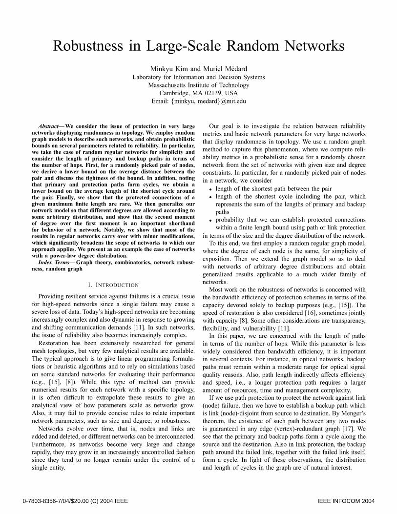
dard method for constructing random regular graphs uniformly[9], [20]. Let V be the set of vertices [n] corresponding ton places along the horizontal axis. For each place in V , weintroduce d vertices and call this two-dimensional set of dnvertices W , W = [n] × [d]. A configuration is a partition ofW into (dn/2) pairs. If we project the setW onto V = [n] bysimply ignoring the second coordinate, we obtain a multigraphπ(F ) where each pair in the configuration is considered anedge (see Fig. 1). However, this is not an ordinary graphbecause it allows loops around the same vertex and multipleedges between two vertices, which, in other words, are cyclesof length 1 and 2, respectively. In particular, if π(F ) lacksthose loops and multiple edges, it is a simple graph which isd-regular. Note that each simple d-regular graph correspondsto precisely (d!)n configurations. Hence, if we choose aconfiguration uniformly at random, conditioned on it beinga simple graph, we get G(n, d) as desired.Connectivity of graphs is a critical issue. If a graph is not

connected initially, then it breaks into several subgraphs, each

...

edge between vertices

[d]

[n]

Fig. 1. Two-Dimensional Set W for Configuration Model

of which is disconnected from the other parts and can be dealtwith as a separate problem. Moreover, if removal of a singleedge or vertex would cause a certain set of source-destinationpairs to be disconnected, then in the corresponding network wehave no viable option to restore the connections but to recoverthe failed link or node itself. Therefore, there is no need toconsider protection for such pairs. However, in random regulargraphs constructed by the configuration model, it is known thatsuch a phenomenon does not happen as n grows large.For an event En, we say that En holds asymptotically almost

surely (a.a.s.) if Pr(En)→ 1 as n tends to infinity. Then, wehave the following result regarding connectivity [19]:Theorem 2.1: If d ≥ 3 and fixed, then G(n, d) is a.a.s.

d-connected.Note that we say a graph is d-connected if, for any pair ofvertices i and j, there is a path connecting i and j in everysubgraph obtained by deleting (d−1) vertices other than i andj together with their adjacent edges from the graph. Therefore,for sufficiently large n, we still get a connected graph afterremoving (d− 1) vertices from G(n, d) for d ≥ 3.Now, let us consider the distribution of cycles in a graph.

Define a random variable Zk to be the number of cycles oflength k in G(n, d). It is known that, for any set of k’s thatare fixed and k ≥ 3, Zk’s are asymptotically distributed asindependent Poisson random variables [3]. More precisely,Theorem 2.2: For each fixed j, a sequence of

random variables (Z3, Z4, ..., Zj) converges a.a.s. to(Z3∞, Z4∞, ..., Zj∞), where {Zk∞}jk=3 is a sequence ofindependent Poisson distributed random variables withE(Zk∞) = (d−1)k

2k .Note, however, that the previous theorem applies only for

cycles of fixed length, that is, where the length of cycle doesnot grow with n. The case of long cycles of which length k isdefined as a function of n, i.e., k = k(n), is considered morerecently by Garmo [7]. By counting the number of cycles onthe two-dimensional set W = [n] × [d] and using Stirling’sformula, Garmo calculates E(Zk), k = 3, ..., n, as follows:Lemma 2.3: Let k be an integer, 3 ≤ k ≤ n, and λ = k/n.

Then,

E(Zk) =(d− 1)k2k

1

exp{12(d−2d k − 1)λ+O(kλ2)}+O( 1n).


d nodes d(d-1) nodes

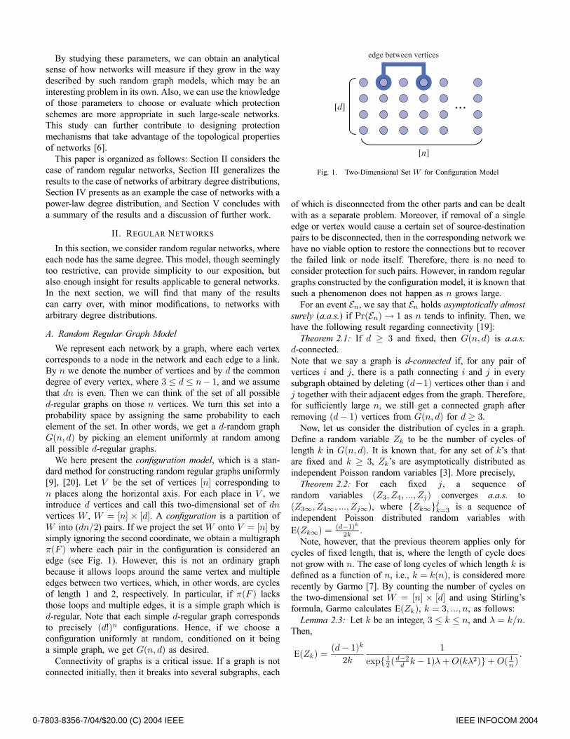
k hops away. . . . . . d+d(d-1)+...+d(d-1)k-1

d{(d-1)k-1}__________ d-2

nodes=

Fig. 2. Maximum Number of Nodes Within k Hops of s

In the above lemma, if k is fixed, then λ → 0 as n tendsto infinity, and thus E(Zk) → (d−1)k

2k as shown in Theorem2.2. On the other hand, if k grows with n, the exponent termsin the denominator, 12(

d−2d k − 1)λ + O(kλ2), are no longer

negligible, which leads E(Zk) to become smaller than (d−1)k2k .

Therefore, we see that (d−1)k

2k is an upper bound on E(Zk)valid for all k, 3 ≤ k ≤ n.We will use these asymptotic results in the following discus-

sion to quantify the reliability issues of networks representedby the configuration model.

B. Shortest PathThroughout the remainder of this section, we assume that

our network is a large random network which is d-regulargraph generated by the configuration model. Suppose n, thenumber of nodes, is large enough so that all the asymptoticproperties in the previous section are assumed to hold, i.e., thedeviation from the asymptotic behavior is assumed negligible.Before proceeding, we present an important property of the

model that we will use in further analysis. If we pick a pair ofnodes randomly and define a random variable X representingsome parameter related to the pair, e.g., the distance betweenthe pair, then there are two sources of randomness: one is therandom selection of a graph and the other is the random pairselection. However, note that, by the symmetric structure ofthe configuration model, the value of X has no dependenceon a specific pair. Hence, calculating the expectation of Xwhich is over the probability space of the selection of a graphis not affected by averaging X again over the selection of apair. Furthermore, by interchanging the order of calculation,we obtain a more convenient way to compute the expectationof X – that is, first conditioning on some graphs to get theexpected value ofX over the pair selection and then averagingthe expectation over all graphs.Let us fix a randomly chosen pair of nodes, s and t, and

define a random variable L to be the length of the shortestpath between s and t. Then, as argued above, assume that wehave a certain d-regular graph and consider the value of Lover the possible selections of a pair.It is clear that there are d nodes adjacent to s. If we consider

the nodes two hops away from s, there can be at most d(d−1) such nodes, but some of them may overlap and therefored(d − 1) is an upper bound on the number of such nodes.Now if we count the total number of nodes within two hops

of s, some nodes adjacent to s and some nodes two hopsaway from s may again overlap, but still there can be at mostd+d(d−1) = d2 such nodes if all of them are distinct. If wecontinue this counting, the number of nodes within k hops ofs is at most d+ d(d− 1) + d(d− 1)2 + · · ·+ d(d− 1)k−1 =d{(d−1)k−1}/(d−2) (see Fig. 2). Note that, in the probabilityspace of the pair selection, Pr(L ≤ k) is the probability thatwe pick another node t among those nodes within k hops ofs. Hence,

Pr(L ≤ k) ≤ min[1,µd{(d− 1)k − 1}

d− 2 · 1

n− 1¶].

Note that this argument is independent of the selection of agraph and thus the above inequality holds for every d-regulargraph. Therefore,

E(L) =n−1Xk=1

(1− Pr(L ≤ k))

≥dlogd−1 neX

k=1

(1− d{(d− 1)k − 1}d− 2 · 1

n− 1)

∼ logd−1 n, (1)

where we assume that n is large.For comparison, let us consider a related result by Newman

et al. [14]. They give an asymptotic heuristic estimate of thetypical length L of the shortest path between two randomlychosen nodes as follows:

L =log[(n− 1)(d2 − 2d) + d2]− log d2

log(d− 1)∼ logd−1 n.

They also note that this approximation may not be correct if allthe vertices are not reachable from a randomly chosen vertex.However, if d ≥ 3, we know that G(n, d) is a.a.s. d-connected,and hence, we can expect that the above approximationbecomes tight as n tends to infinity.Comparing this to the lower bound (1), we find that our

lower bound matches the existing estimate for large n, andthis may be viewed as an indication of its tightness.

C. Shortest CycleRecall that cycles are of our interest because primary and

backup paths together form a cycle in a graph. In this section,we also consider a randomly picked pair of nodes, and nowwe define the random variable X as the length of the shortestcycle including the pair.Now we define an event Yk that the pair is on a k-cycle

(cycle of length k), i.e., there exists a k-cycle through thetwo nodes. Then, by the definition of X, X ≤ k implies thepair is on a certain cycle no longer than k and we obtain thefollowing inequality:

Pr(Yk) ≤ Pr(X ≤ k) ≤kXi=3

Pr(Yi), (2)


where we used the union bound for an upper bound. Therefore,we can lowerbound E(X) as follows:

E(X) =nX

k=3

kPr(X = k)

≥m−1Xk=3

k{Pr(X ≤ k)− Pr(X ≤ k − 1)}

+m(1− Pr(X ≤ m− 1)) (3)

≥m−1Xk=3

k{Pr(Yk)−k−1Xj=3

Pr(Yj)}

+m(1−m−1Xj=3

Pr(Yj)) (4)

= m−m−1Xk=3

Pr(Yk){mX

j=k+1

j − k}, (5)

wherem is an integer, 4 ≤ m ≤ n. Note in (3) that, for each klarger than m, we replaced kPr(X = k) by mPr(X = k) toget a lower bound, and that (4) follows from (2). Since in (5)each Pr(Yk) is multiplied by a negative number, if we obtaina lower bound on Pr(Yk), we can further bound E(X) frombelow.Now define an indicator random variable Ik taking 1 if the

pair is on a k-cycle, and 0, otherwise. To calculate E(Ik), asmentioned above, we first condition on a certain graph andconsider a pair selection on the graph, and then average theresult over all graphs. More specifically, if we define Zk tobe the number of k-cycles in a graph, conditioned on Zk = j,we calculate conditional expectation of Ik by considering arandom selection of a pair of nodes, which we average overall possible values of Zk. Identifying E(Ik) as equivalent toPr(Yk), we can write this calculation as follows:

Pr(Yk) =Xj

E(Ik|Zk = j)Pr(Zk = j)

=Xj

Pr(Yk|Zk = j)Pr(Zk = j), (6)

where the expectation and probability conditioned on Zk areover the probability space of pair selection.Let us consider how we can maximize the conditional

probability Pr(Yk|Zk = j), i.e., the probability that the pairis on a k-cycle given that the graph has a certain number ofk-cycles. If we assume there is a total of n nodes,

Pr(Yk|Zk = j) =(number of pair selections on k-cycle)¡

n2

¢ .

(7)In order to calculate the maximum number of pair selectionson a k-cycle, we first take the case of two cycles. If the twocycles are disjoint, i.e. they share no vertex, the number ofsuch selections is 2

¡k2

¢. We obtain the same result when there

is only one vertex shared by the two cycles. However, if thetwo cycles share j vertices, where 2 ≤ j ≤ k − 1, then thenumber of pair selections on a k-cycle is 2

¡k2

¢− ¡j2¢, which is

4 6 8 10 12 14 16 18 20 22 242

4

6

8

10

12

14

16

18

20

Low

er B

ound

on

E(X

)

Value of m where Truncation Starts

d=3d=4d=5

Fig. 3. Lower Bound on E(X) with respect to m for n = 10, 000

strictly less than that of the previous case. Hence, we get themaximum number of pair selections when the two cycles shareno or only one vertex. Note that by repeating this argument, theresult easily extends to the case of more than two cycles. Thatis, if we have j cycles of length k, by assuming all the cyclesare disjoint, we can maximize the number of pair selectionson a k-cycle, which is given by j

¡k2

¢. Hence, it follows from

(6) and (7) that

Pr(Yk) ≤Xj

j¡k2

¢¡n2

¢ Pr(Zk = j)

=k(k − 1)n(n− 1)E(Zk). (8)

Now, recall that, as discussed in Section II-A, we have anupper bound on E(Zk) for any k, 3 ≤ k ≤ n, such that

E(Zk) ≤ (d− 1)k

2k.

Therefore,

Pr(Yk) ≤ (k − 1)2n(n− 1)(d− 1)

k. (9)

Combining (5) and (9), we obtain

E(X) ≥m−m−1Xk=3

(k − 1)(d− 1)k2n(n− 1) {

mXj=k+1

j − k}, (10)

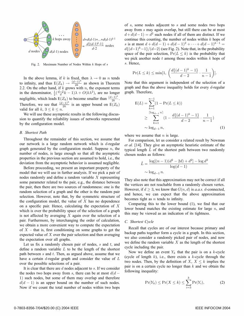
which is valid for any m, 4 ≤ m ≤ n. We can calculate thislower bound numerically for various m. In Fig. 3, we noticethat the bound grows until some value of m, where we obtainthe tightest lower bound, and then it starts to decrease as mfurther grows.We can collect these lower bounds for each n, which Fig.

4 plots with respect to logn, for n up to 1030. Interestingly,those bounds are shown to grow almost linearly with logn,which is in turn congruent to the lower bound (Eq. (1)) on thepath length in the previous section.


0 5 10 15 20 25 300

20

40

60

80

100

120

140

160

180

200Lo

wer

Bou

nd o

n E

(X)

log10(n)

d=3d=4d=5

Fig. 4. Lower Bound with respect to logn

This can be explained analytically as well. For fixed d andm = m(n) that grows with n, let B be the terms on theright-hand side in (10). Then, by using manipulation of series,

B =m−m−1Xk=3

(k − 1)(d− 1)k2n(n− 1) {

mXj=k+1

j − k}

=m− 1

n2·Θµm−1X

k=3

m2k(d− 1)k − k3(d− 1)k¶

=m− 1

n2·Θ(m3(d− 1)m). (11)

Let us suppose that m = c logn for a constant c > 0, wherewe can infer, by examining the value of m that gives thetightest lower bound for each n in Fig. 3, that the maximummay occur when m is approximately order of logn. Then,Θ(m3(d − 1)m) = Θ((c logn)3 · nc log(d−1)). Hence, if c <

2log(d−1) , then B ∼ c logn since Θ(m3(d − 1)m)/n2 → 0.Otherwise, if c ≥ 2

log(d−1) , then B tends to below zero sincethe term Θ(m3(d − 1)m)/n2 with a minus sign dominatesin B. Also, we can show that if m

logn → 0 or mlogn → ∞,

then B = Θ(m) or B → −∞, respectively. Therefore, weconclude that the best case is when B = Θ(logn), which isthe tightest lower bound on E(X).We also notice that, since the tightest lower bound occurs

when c ≈ 2log(d−1) , the resulting bound is approximately

2 logd−1 n. Therefore, the lower bound on the shortest cycleturns out to be roughly twice the lower bound on the shortestpath we obtained for regular graphs.

D. Probability of Short CycleSuppose we want to maintain the path lengths below a

certain level in terms of the number of hops, for the reasonsmentioned in Section I. Let a finite number lmax denote themaximum length of the paths allowed, and we want to computethe probability that we can protect the traffic using only suchpaths.

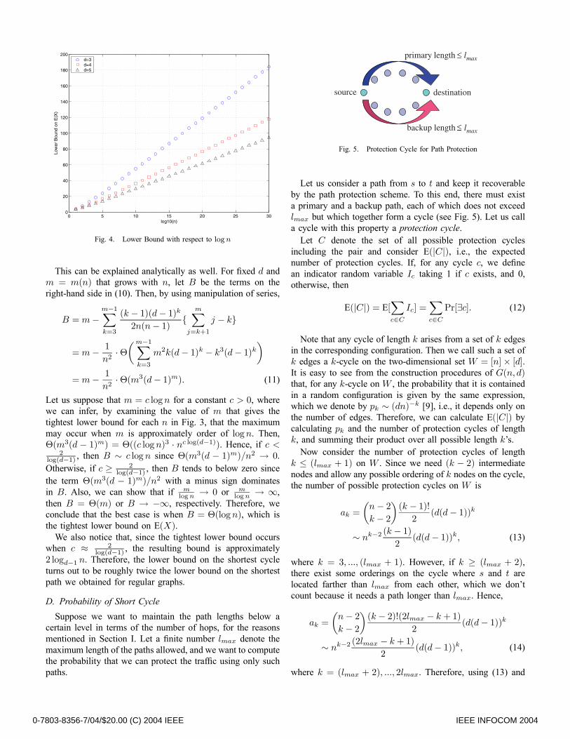
source destination

primary length lmax

backup length lmax

Fig. 5. Protection Cycle for Path Protection

Let us consider a path from s to t and keep it recoverableby the path protection scheme. To this end, there must exista primary and a backup path, each of which does not exceedlmax but which together form a cycle (see Fig. 5). Let us calla cycle with this property a protection cycle.Let C denote the set of all possible protection cycles

including the pair and consider E(|C|), i.e., the expectednumber of protection cycles. If, for any cycle c, we definean indicator random variable Ic taking 1 if c exists, and 0,otherwise, then

E(|C|) = E[Xc∈C

Ic] =Xc∈C

Pr[∃c]. (12)

Note that any cycle of length k arises from a set of k edgesin the corresponding configuration. Then we call such a set ofk edges a k-cycle on the two-dimensional set W = [n]× [d].It is easy to see from the construction procedures of G(n, d)that, for any k-cycle on W , the probability that it is containedin a random configuration is given by the same expression,which we denote by pk ∼ (dn)−k [9], i.e., it depends only onthe number of edges. Therefore, we can calculate E(|C|) bycalculating pk and the number of protection cycles of lengthk, and summing their product over all possible length k’s.Now consider the number of protection cycles of length

k ≤ (lmax + 1) on W . Since we need (k − 2) intermediatenodes and allow any possible ordering of k nodes on the cycle,the number of possible protection cycles on W is

ak =

µn− 2k − 2

¶(k − 1)!2

(d(d− 1))k

∼ nk−2(k − 1)2

(d(d− 1))k, (13)

where k = 3, ..., (lmax + 1). However, if k ≥ (lmax + 2),there exist some orderings on the cycle where s and t arelocated farther than lmax from each other, which we don’tcount because it needs a path longer than lmax. Hence,

ak =

µn− 2k − 2

¶(k − 2)!(2lmax − k + 1)

2(d(d− 1))k

∼ nk−2(2lmax − k + 1)

2(d(d− 1))k, (14)

where k = (lmax + 2), ..., 2lmax. Therefore, using (13) and


(14), we obtain

E(|C|) =2lmaxXk=3

akpk

∼lmax+1Xk=3

(k − 1)(d− 1)k2n2

+2lmaxX

k=lmax+2

(2lmax − k + 1)(d− 1)k2n2

=2lmaxXk=3

(d− 1)k2n2

min[k − 1, 2lmax − k + 1].

If we consider the probability that there exists at least aprotection cycle along the pair of nodes, it is bounded fromabove by E(|C|), which is a union bound including all possibleprotection cycles, and from below by the probability that thereexists a cycle of length 3 on W . Hence,

1

(dn)3≤Pr(∃protection cycle)

≤2lmaxXk=3

(d− 1)k2n2

min[k − 1, 2lmax − k + 1].

In the case of link protection, if we assume that there is alink between s and t, in order to ensure that traffic betweenthe pair is recoverable by the link protection scheme, theremust exist a cycle not exceeding (lmax + 1) around the pair.In exactly the same manner, we can calculate the expectednumber of such cycles around the pair. Hence, in the linkprotection case, we can bound the probability that there existsat least one protection cycle of length within a finite bound asfollows:

1

(dn)3≤ Pr(∃protection cycle) ≤

lmax+1Xk=3

(d− 1)k2n2

.

Note from the results above that, for both path and linkprotection schemes, the probability that we find a backup pathof finite length decays in the order of 1

n2 . In other words, inthe random networks described by the configuration model, itis highly unlikely to find a backup path within a finite rangeas the size of network grows very large.

III. GENERAL NETWORKSIn this section, we present an extended version of the

configuration model, by which we can overcome the limitationthat the degree must be the same over all nodes. Then we showthat most of our results for regular graphs carry over to moregeneral networks based on the extended model.

A. Extended Graph ModelMolloy and Reed [12] and Newman et al. [14] present a

random graph model with a given degree sequence, but theydo not consider explicitly the randomization of degrees with agiven degree distribution. Aiello et al. [1] use the same modelas that we discuss here, however their analyses are limited to a

...

edge between vertices

[Di]

[n]

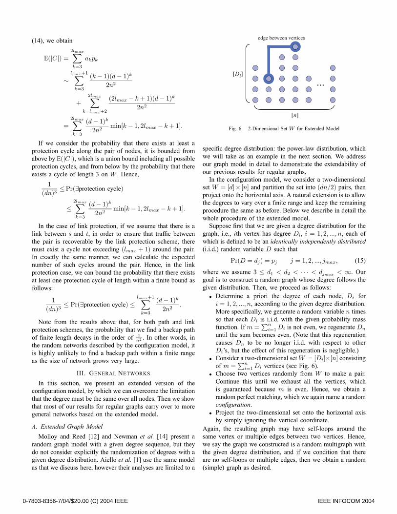
Fig. 6. 2-Dimensional Set W for Extended Model

specific degree distribution: the power-law distribution, whichwe will take as an example in the next section. We addressour graph model in detail to demonstrate the extendability ofour previous results for regular graphs.In the configuration model, we consider a two-dimensional

set W = [d]× [n] and partition the set into (dn/2) pairs, thenproject onto the horizontal axis. A natural extension is to allowthe degrees to vary over a finite range and keep the remainingprocedure the same as before. Below we describe in detail thewhole procedure of the extended model.Suppose first that we are given a degree distribution for the

graph, i.e., ith vertex has degree Di, i = 1, 2, ..., n, each ofwhich is defined to be an identically independently distributed(i.i.d.) random variable D such that

Pr(D = dj) = pj j = 1, 2, ..., jmax, (15)

where we assume 3 ≤ d1 < d2 < · · · < djmax < ∞. Ourgoal is to construct a random graph whose degree follows thegiven distribution. Then, we proceed as follows:• Determine a priori the degree of each node, Di fori = 1, 2, ..., n, according to the given degree distribution.More specifically, we generate a random variable n timesso that each Di is i.i.d. with the given probability massfunction. If m =

Pni=1Di is not even, we regenerate Dn

until the sum becomes even. (Note that this regenerationcauses Dn to be no longer i.i.d. with respect to otherDi’s, but the effect of this regeneration is negligible.)

• Consider a two-dimensional setW = [Di]×[n] consistingof m =

Pni=1Di vertices (see Fig. 6).

• Choose two vertices randomly from W to make a pair.Continue this until we exhaust all the vertices, whichis guaranteed because m is even. Hence, we obtain arandom perfect matching, which we again name a randomconfiguration.

• Project the two-dimensional set onto the horizontal axisby simply ignoring the vertical coordinate.

Again, the resulting graph may have self-loops around thesame vertex or multiple edges between two vertices. Hence,we say the graph we constructed is a random multigraph withthe given degree distribution, and if we condition that thereare no self-loops or multiple edges, then we obtain a random(simple) graph as desired.


Note that in this model, by setting the minimum degree to beat least three, we can restrict ourselves to considering verticesof degree no less than three. Let us justify this exclusion in thecontext of protection in communication networks. For a nodeof degree one, there is only one link connecting the node tothe network. Hence, if the link fails, there is no way but tosimply fix the failed link to recover the connection. Also, itis easy to see that we cannot establish two link-disjoint pathsstarting or ending at a node of degree one. Hence, we do notneed to consider nodes of degree one explicitly in both linkand path protection.For nodes of degree two, any such node should fall in the

middle of links between a different pair of nodes. Hence, evenif we ignore a node of degree two and merge its two links intoone, there will be no changes in the topological structure ofthe network. Hence, in considering the asymptotic behaviorof the length of paths, we can ignore nodes of degree twoand later, if needed, we can add such nodes according to anappropriate distribution, which can be handled in a separateproblem.Regarding connectivity, [19] shows that a graph with any

given collection of degrees lying between r and R, 3 ≤r ≤ R ≤ ∞, is a.a.s. r-connected. Hence, if dmin ≥ 3is the minimum degree that each node can take, graphsconstructed by the extended configuration model are a.a.s.dmin-connected.

B. Distribution of the Number of CyclesWe recall that the number of k-cycles in random regular

graphs is asymptotically Poisson distributed. Interestingly, thisproperty carries over to the case of general networks based onthe extended model. Let the distribution of degree D be givenas in (15) and denote the resulting graph by Ge(n,D). Thenwe obtain the following theorem:Theorem 3.1: Let Zk be the number of cycles of length k

in Ge(n,D). For each fixed j, a sequence of random variables(Z3, Z4, ..., Zj) converges a.a.s. to (Z3∞, Z4∞, ..., Zj∞),where {Zk∞}jk=3 is a sequence of independent Poisson dis-tributed random variables with E(Zk∞) = 1

2k (E(D2)E(D) − 1)k.

Proof outline: Details of the proof are omitted for lack of spacebut can be found in [10]. This is an extension of the proofof the distribution of short cycles in random regular graphs[9]. First, consider a random multigraph with the given degreedistribution. By conditioning on the number of nodes withdegree di and using the strong law of large numbers, we cancalculate each factorial moment. Averaging the results basedon the degree distribution, we can show that each factorialmoment converges a.a.s. to that of the desired joint Poissonrandom variables. Since Zi’s are independent, the distributionsremain unchanged after conditioning Z1 = Z2 = 0. Hence, theresult for a simple graph follows. ¤Note that the above theorem holds only for fixed-length

cycles. For length k which grows with n, we show that theexpression of E(Zk) for fixed k is an upper bound on E(Zk),i.e.,

Lemma 3.2:

E(Zk) ≤ 1

2k

µE(D2)

E(D)− 1¶k

,

for 3 ≤ k ≤ n.Proof outline: A full derivation is omitted due to spacelimitations but also can be found in [10]. Even for k = k(n),by considering the corresponding two-dimensional set, we cancalculate the mean number of k-cycles exactly in a closed-form, which is, however, complicated. Applying Stirling’sformula, we obtain a simpler asymptotic expression, and wecan show that the desired inequality finally reduces to the log-sum inequality. ¤We see that the crucial characteristic here is the second

moment of degree over the first moment, {E(D2)/E(D)},which plays the same role as the degree in regular graphs(see Theorem 2.2). As we will see later, this parameter alsohas a crucial impact on the length of path and cycle.

C. Shortest PathThroughout the remainder of this section, we consider a

large network represented by a random graphGe(n,D), whichis generated by the extended configuration model with suffi-ciently large n and the given degree distribution D satisfyingthe properties discussed in Section III-A.Let us fix a randomly chosen pair of nodes, s and t, and

define a random variable L to be the length of the shortest pathbetween s and t. As in the previous case of random regulargraphs, Newman et al.’s heuristic approach to a related model[14] also applies to networks of general degree distribution,and we will discuss how their asymptotic estimate of typicallength L relates to our results.For a graph constructed by our model with general degree

distribution D, L is given in [14] by

L =log[{(n− 1)(E(D2)− 2E(D)) + E(D)2}/E(D)2]

log[(E(D2)− E(D))/E(D)](16)

and if nÀ E(D) and E(D2)À E(D), this reduces to

L =log( n

E(D))

log(E(D2)

E(D) − 1)+ 1. (17)

Interestingly, the second moment of degree over the firstmoment is also crucial here. As we increase the varianceof degrees while maintaining the same mean degree, wehave shorter L. On the other hand, as pointed out in [14],two random graphs with completely different distributions ofdegrees, but the same value of the second moment of degreeover the first moment, will have asymptotically the same meanpath length.

D. Shortest CycleAs before, we now consider a random variableX, defined to

be the length of the shortest cycle including a randomly pickedpair of nodes. We will show that the procedures for deriving alower bound on E(X) for regular graphs apply here with slight


modifications, which is expected because we can see that mostof the previous results do not depend on the fact that graphsare regular. For comprehensiveness, we recast important stepsin the derivation, but also for conciseness, we omit details ifthere is no major change compared with the case of regulargraphs.If we let Yk be the event that the pair is on a k-cycle, i.e.,

there exists a k-cycle around the pair, then, for any integer m,4 ≤m ≤ n,

E(X) ≥ m−m−1Xk=3

Pr(Yk){mX

j=k+1

j − k}. (18)

Also, we have the same expression as in (8) for an upperbound on Pr(Yk) such that

Pr(Yk) ≤ k(k − 1)n(n− 1)E(Zk).

Applying Lemma 3.2, we have, for graphs with a generaldegree distribution D,

Pr(Yk) ≤ (k − 1)2n(n− 1)

µE(D2)

E(D)− 1¶k

. (19)

Hence, from (18) and (19), we obtain the following lowerbound on E(X):

E(X) ≥m−m−1Xk=3

(k − 1)(E(D2)E(D) − 1)k

2n(n− 1) {mX

j=k+1

j − k}. (20)

By similar numerical calculation and convergence analysis asin Section II-C, we conclude that the above bound is O(logn).It is very interesting to see that, since it is multiplied

by a negative value, as {E(D2)/E(D)} increases we havea smaller bound on E(X). Note that this fact is consistentwith the results in the previous two sections: a larger value of{E(D2)/E(D)} yields shorter L (Eq. (17)) and more cycles(Theorem 3.1). This observation meets our expectation that,as the number of cycles increases, the length of the shortestcycle including a pair of nodes as well as the distance betweenthe pair decreases.Hence, the second moment of degree over the first moment

should be dealt with as a special parameter that determines theasymptotic behavior of both the average length of paths andcycles, and the average number of cycles in random graphs.

E. Finite Length CycleLet a finite number lmax denote the maximum length of the

paths allowed, and let us compute bounds on the probabilitythat we can protect the network using only such paths. Again,if there is no major change in the argument compared withthe case of regular graphs, we omit details and present onlyimportant steps.For path protection, we define a protection cycle as before,

i.e., a cycle consisting of a primary and a backup path, eachof which does not exceed lmax, from s to t. To computethe probability that there exists at least one protection cycle,we consider E(|C|) where C denotes the set of all possible

protection cycles including the pair. Similarly as in regulargraphs, we can calculate E(|C|) by counting the number ofappropriate cycles in the two-dimensional set of the extendedconfiguration model. A full derivation can be found in [10].Owing to space limitations we present only the result here.

E(|C|) ∼2lmaxXk=3

1

2n2

µE(D2)

E(D)− 1¶k

×min[k − 1, 2lmax − k + 1]. (21)

If we consider the probability that there exists at least oneprotection cycle along the pair of nodes, it is bounded fromabove by E(|C|), which is a union bound including all possibleprotection cycles, and from below by the probability that thereexists a cycle of length 3 on W . Therefore,

1

(nE(D))3≤Pr(∃protection cycle)

≤2lmaxXk=3

1

2n2

µE(D2)

E(D)− 1¶k

×min[k − 1, 2lmax − k + 1].

Now, for link protection, assume there is a link between sand t. To ensure that traffic between the pair is recoverableby the link protection scheme, there must exist a cycle notexceeding (lmax + 1) around the pair. As in path protection,we calculate the expected number of such cycles around thepair and bound the probability that there exists at least oneprotection cycle of length within a finite bound as follows:

1

(nE(D))3≤ Pr(∃protection cycle)

≤lmax+1Xk=3

1

2n2

µE(D2)

E(D)− 1¶k

.

Note from the results above that, also in random graphsof a general degree distribution, the probability that we finda backup path of finite length decays in the order of 1

n2 forboth path and link protection schemes. In other words, it ishighly unlikely to find a backup path within a finite range asthe size of the network grows very large.

IV. EXAMPLE: POWER-LAW DEGREE DISTRIBUTIONIn this section, we take as an example the case of networks

with a power-law degree distribution, which is often used as adescription of large complex networks. Our aim here is not todiscuss the validity of the power-law model, but to illustratethe flexibility and usefulness of our method by applying it toan existing model that is commonly used.A considerable number of studies have been carried out

on the structures and properties of many kinds of real-worldcomplex network, e.g., [2], [18]. A very common result is that,in most real-world networks, the degree distribution is highlyright-skewed, i.e., it has a long right tail of values that arefar above the mean [13]. More specifically, it is often of the


form pk ∼ k−α for some positive constant α, which is calleda power-law distribution.Despite the extensive research on various types of complex

networks, there is a very limited amount of literature focusingmainly on communication networks, where the issue of pro-tection is of critical importance. Among those few studied,a frequently considered network is the Internet. Faloutsoset al. [6] discover that several parameters of the Internetgraph, such as outdegrees of a node or eigenvalues, displaypower-law distributions. However, more recently Chen et al.[4] show that, by using a different method for obtainingthe Internet graph, degree distributions of the Internet graphsare also heavy-tailed but deviate significantly from a strictpower-law. These observations indicate that, in consideringcommunication networks, we do not need to limit ourselvesto networks with the degree distribution of a power-law.Now, let us consider networks with the degree distribution

defined as

Pr(D = k) =

(0 for 0 ≤ k ≤ 2k−α/c for 3 ≤ k ≤ kmax,

for given constant α. Here kmax is an often-used approximateof the maximum degree [13], given by kmax = n1/(α−1), and cis a normalizing constant, given by c =

Pkmax

k=3 k−α. Note thatthis distribution is different from a strict power-law distributionin that nodes of degree below three are ignored for the reasonsdiscussed in Section III-A. Also, this analysis is approximate– the degree constraint of our model is not precisely satisfiedsince here the maximum degree is a function of n, althoughthe probability of such nodes decays significantly. Within thebest of our knowledge, the overall effect of the unboundedmaximum degree in graphs with a general degree distributionis not known precisely.For networks of this degree distribution, Fig. 7 plots with

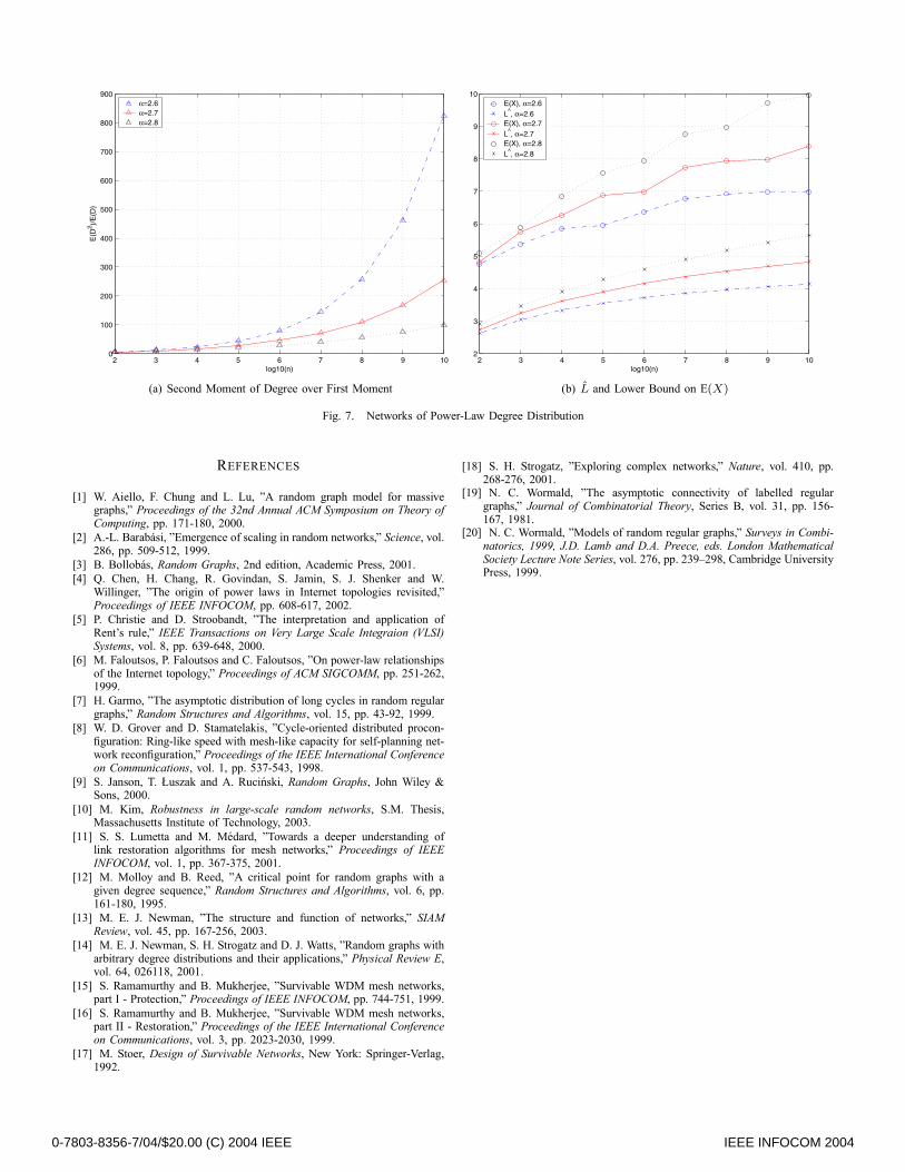
respect to logn the parameters that we have considered. Wechoose three different α’s around the experimental values in[6]. In particular, Fig. 7(a) shows the second moment of degreeover the first moment of degree, which as we have discussedabove closely relates to the average number of cycles as wellas the average path/cycle length. We find that the value of thesecond moment of degree over the first moment increases withn, but decreases with α. In Fig. 7(b), we plot the asymptoticheuristic estimate of typical distance, L (Eq. (16)), and thelower bound on the expected length of the shortest cycleincluding a randomly picked pair of nodes, E(X) (Eq. (20)).Here we see that, as we discussed before, those two parametersdecrease as {E(D2)/E(D)} increases for the same n.One may notice that those parameters produce surprisingly

small values for the size of the network. Recall that the secondmoment of degree over the first moment is a crucial parameterthat determines the asymptotic behavior of a network. Forcycle length, this parameter corresponds exactly to the degreein a regular network (see (20) and (10)). For instance, if α =2.6 and n = 1010, the network shows the characteristics of aregular graph with degree 825. This large value results partlyfrom the fact that we ignore the nodes of degree less than three,

and if we calculate the parameter again including the nodesof degree one and two, we now have 345, still a large value.Hence, we conclude that this property of high-connectivityand short path/cycle lengths is an inherent characteristic ofnetworks with a power-law degree distribution.Note, however, that we do not intend to suggest that the

power-law distribution is appropriate for large-scale networksin practice, nor that our approach is limited to power-lawdistributed networks. Rather, we have shown that our approachis applicable to estimating the length of backup paths ingeneral networks of arbitrary degree distributions.

V. CONCLUSIONSWe have investigated the issue of protection in large-scale

random networks by deriving several bounds on the parametersrelated to protection in terms of network parameters, such assize and degree. We first considered random regular networksdescribed by the configuration model, and derived bounds onthe mean path and cycle length and also the probability offinite-length protected connections. We then extended theseresults to general networks with arbitrary degree distributions.We presented the distribution of the number of fixed-lengthcycles and derived an upper bound on the mean number ofcycles of non-finite length. We found the second moment ofdegree over the first moment is a crucial parameter for theasymptotic behavior of a network.The main contributions of this study are the following. First,

we took an analytical approach toward the study of networkprotection by bringing the concept of randomness into net-work topologies. Our approach is crucial to understanding therelation between reliability metrics, such as connectivity andlength of backup paths, and basic network parameters, suchas degree distribution and network size, for large networks.In addition, we established analytical results for the lengthof backup paths for path and link-based protection schemes.These results, though not complete yet, allow us to understandthe applicability of standard protection preplanned approaches.Finally, we developed a unified framework for studying theissue of robustness in very general networks with arbitrarydegree distributions.There are several topics for further research. Our results

indicate that both the shortest path and cycle between a pair ofnodes may scale logarithmically with the size of the network.A formal analysis of the validity of this claim would be useful.Furthermore, we may extend our network model to allow timevariability of networks that are evolving dynamically, whichmay provide an analytical tool for developing or evaluatingspecific algorithms or protocols for protection. The networkmodel may be also modified to allow some dependency onproximity or localization, for instance to satisfy Rent’s rule[5], or to explain transitivity or clustering in a network [13].

ACKNOWLEDGMENTThe authors would like to thank Douglas B. West, R. Srikant

and Supratim Deb at the University of Illinois at Urbana-Champaign for helpful discussions.


2 3 4 5 6 7 8 9 100

100

200

300

400

500

600

700

800

900

log10(n)

E(D

2 )/E

(D)

α=2.6α=2.7α=2.8

(a) Second Moment of Degree over First Moment

2 3 4 5 6 7 8 9 102

3

4

5

6

7

8

9

10

log10(n)

E(X), α=2.6L^, α=2.6E(X), α=2.7L^, α=2.7E(X), α=2.8L^, α=2.8

(b) L and Lower Bound on E(X)

Fig. 7. Networks of Power-Law Degree Distribution

REFERENCES

[1] W. Aiello, F. Chung and L. Lu, ”A random graph model for massivegraphs,” Proceedings of the 32nd Annual ACM Symposium on Theory ofComputing, pp. 171-180, 2000.

[2] A.-L. Barabasi, ”Emergence of scaling in random networks,” Science, vol.286, pp. 509-512, 1999.

[3] B. Bollobas, Random Graphs, 2nd edition, Academic Press, 2001.[4] Q. Chen, H. Chang, R. Govindan, S. Jamin, S. J. Shenker and W.

Willinger, ”The origin of power laws in Internet topologies revisited,”Proceedings of IEEE INFOCOM, pp. 608-617, 2002.

[5] P. Christie and D. Stroobandt, ”The interpretation and application ofRent’s rule,” IEEE Transactions on Very Large Scale Integraion (VLSI)Systems, vol. 8, pp. 639-648, 2000.

[6] M. Faloutsos, P. Faloutsos and C. Faloutsos, ”On power-law relationshipsof the Internet topology,” Proceedings of ACM SIGCOMM, pp. 251-262,1999.

[7] H. Garmo, ”The asymptotic distribution of long cycles in random regulargraphs,” Random Structures and Algorithms, vol. 15, pp. 43-92, 1999.

[8] W. D. Grover and D. Stamatelakis, ”Cycle-oriented distributed procon-figuration: Ring-like speed with mesh-like capacity for self-planning net-work reconfiguration,” Proceedings of the IEEE International Conferenceon Communications, vol. 1, pp. 537-543, 1998.

[9] S. Janson, T. Łuszak and A. Rucinski, Random Graphs, John Wiley &Sons, 2000.

[10] M. Kim, Robustness in large-scale random networks, S.M. Thesis,Massachusetts Institute of Technology, 2003.

[11] S. S. Lumetta and M. Medard, ”Towards a deeper understanding oflink restoration algorithms for mesh networks,” Proceedings of IEEEINFOCOM, vol. 1, pp. 367-375, 2001.

[12] M. Molloy and B. Reed, ”A critical point for random graphs with agiven degree sequence,” Random Structures and Algorithms, vol. 6, pp.161-180, 1995.

[13] M. E. J. Newman, ”The structure and function of networks,” SIAMReview, vol. 45, pp. 167-256, 2003.

[14] M. E. J. Newman, S. H. Strogatz and D. J. Watts, ”Random graphs witharbitrary degree distributions and their applications,” Physical Review E,vol. 64, 026118, 2001.

[15] S. Ramamurthy and B. Mukherjee, ”Survivable WDM mesh networks,part I - Protection,” Proceedings of IEEE INFOCOM, pp. 744-751, 1999.

[16] S. Ramamurthy and B. Mukherjee, ”Survivable WDM mesh networks,part II - Restoration,” Proceedings of the IEEE International Conferenceon Communications, vol. 3, pp. 2023-2030, 1999.

[17] M. Stoer, Design of Survivable Networks, New York: Springer-Verlag,1992.

[18] S. H. Strogatz, ”Exploring complex networks,” Nature, vol. 410, pp.268-276, 2001.

[19] N. C. Wormald, ”The asymptotic connectivity of labelled regulargraphs,” Journal of Combinatorial Theory, Series B, vol. 31, pp. 156-167, 1981.

[20] N. C. Wormald, ”Models of random regular graphs,” Surveys in Combi-natorics, 1999, J.D. Lamb and D.A. Preece, eds. London MathematicalSociety Lecture Note Series, vol. 276, pp. 239–298, Cambridge UniversityPress, 1999.


Robustness in large-scale random networks

Documents

Transcript of Robustness in large-scale random networks