The Robustness of Exclusion in Multi-dimensional Screening

Paulo Barelli Suren Basov Mauricio Bugarin Ian King

Working Paper No. 571

February 2012

University of

Rochester

The Robustness of Exclusion

in Multi-dimensional Screening

Paulo Barelli Suren Basov Mauricio Bugarin Ian King ∗

February 21, 2012

Abstract

We extend Armstrong’s [2] result on exclusion in multi-dimensional screening mod-

els in two key ways, providing support for the view that this result is generic and

applicable to many different markets. First, we relax the strong technical assumptions

he imposed on preferences and consumer types. Second, we extend the result beyond

the monopolistic market structure to generalized oligopoly settings with entry. We also

analyze applications to several quite different settings: credit markets, the automobile

industry, research grants, the regulation of a monopolist with unknown demand and

cost functions, and involuntary unemployment in the labor market.

JEL Codes: C73, D82

Key words: Multi-dimensional screening, exclusion, regulation of a monopoly,

involuntary unemployment.

1 Introduction

When considering the problem of screening, where sellers choose a sales mechanism and buy-

ers have private information about their types, it is well known that the techniques used in

the multi-dimensional setting are not as straightforward as those in the one-dimensional set-

ting. As a consequence, while we have a host of successful applications with one-dimensional

∗Paulo Barelli: University of Rochester, Suren Basov: La Trobe University, Mauricio Bugarin: Insper

Institute, Ian King: University of Melbourne. We are grateful to Mark Armstrong, Steve Williams, Aloisio

Araujo, the seminar audiences at SAET 2010, Deakin University and Boston University, especially Hsueh-

Ling Huynh, and three anonymous referees for helpful comments.

1

types, to date we have only a few scattered papers that allow for multidimensional types.

This is unfortunate because in many, if not most, economic applications multi-dimensional

types are needed to capture the basic economics of the environment, and the propositions

coming from the one dimensional case do not necessarily generalize to the multi-dimensional

case.1

One of the most well known results in the theory of multi-dimensional screening, though,

comes from Armstrong [2], who shows that a monopolist will find it optimal to not serve some

fraction of consumers, even when there is positive surplus associated with those consumers.

That is, in settings where consumers vary in at least two different ways, monopolists will

choose a sales mechanism that excludes a positive measure of consumers. The intuition

behind this result is rather simple: consider a situation where the monopolist serves all

consumers; if she increases the price by ε > 0 she earns extra profits of order O(ε) on the

consumers who still buy the product, but will lose only the consumers whose surplus was

below ε. If m > 1 is the dimension of the vector of consumers’ taste characteristics, then the

measure of the set of the lost consumers is O(εm). Therefore, it is profitable to increase the

price and lose some consumers. In principle, this result has profound implications across a

wide range of economic settings. The general belief that heterogeneity of consumer types is

likely to be more than one-dimensional in nature, for many different commodities, and that

these types are likely to be private information, underlines the importance of this result.2

However, the result itself was derived under a relatively strong set of assumptions that

could be seen as limiting its applicability, and subsequent research has identified conditions

under which the result does not hold. In particular, Armstrong’s original analysis assumes

that the utility functions of the agents are homogeneous and convex in their types, and

that these types belong to a strictly convex and compact body of a finite dimensional space.

Basov [7] refers to the latter as the joint convexity assumption and argues that, although

convexity of utility in types and convexity of the types set separately are not restrictive and

can be seen as a choice of parametrization, the joint convexity assumption is technically

restrictive.

The joint convexity assumption has no empirical foundation and is nonstandard. For

instance, the benchmark case of independent types fails joint convexity, because the type

space is the not strictly convex multi-dimensional box. There is, in general, no theoretical

1See Rochet and Stole [23] and Basov [7] for surveys of the literature.2The type of an economic agent is simply her utility function. If one is agnostic about the preferences

and does not want to impose on them any assumptions beyond, perhaps, monotonicity and convexity, then

the most natural assumption is that the type is multi-dimensional.

2

justification for a particular assumption about the curvature of utility functions with respect

to types, as opposed to, say, quasi-concavity of utility functions with respect to goods. In

the same line, in general, there is no justification, other than analytical tractability, for type

spaces to be convex, and for utility functions to be homogeneous in types. Both Armstrong [4]

and Rochet and Stole [23] found examples outside of these restrictions where the exclusion

set is empty.

We show that these counter-examples are not generic. We also show that exclusion is

generic under more general market structures, i.e. the result is actually quite robust. We

then provide examples where we believe exclusion is a relevant economic phenomenon.

We start with relaxing the joint convexity and homogeneity assumptions, and show that

they are not necessary for the result. Exclusion is generically optimal in the family of models

where types belong to sets of locally finite perimeter (which is a class of sets that includes

all of the examples the authors are aware of in the literature) and utility functions are

smooth and monotone in types. We show that the examples considered in Armstrong[4]

and Rochet and Stole [23] are, themselves, very special cases. We then go on to show that

the exclusion results can be generalized to the case of an oligopoly and an industry with

free entry. Therefore, the inability of some consumers to purchase the good at acceptable

terms is solely driven by the multi-dimensional nature of private information rather than by

market conditions or the nature of distribution of consumers’ tastes.

To illustrate the generality of the results, we apply them in several different settings:

credit markets, the automobile industry, and research grants. We also pay particular at-

tention to two applications: the first being the regulation of a monopolist with unknown

demand and cost functions, and the second being the existence of equilibrium involuntary

unemployment. The former application picks up of the analysis in Armstrong [4], where

he reviews Lewis and Sappington [17] and conjectures that exclusion is probably an issue

in their analysis. At the time, Armstrong could not prove the point, due to the lack of a

more general exclusion result. With our result in hand, we are able to prove Armstrong’s

conjecture. The latter application is a straightforward way of showing that, when workers

have multi-dimensional characteristics, it is generically optimal for employers (with market

power in the labor market) to not hire all the workers.

Most generally, we believe that the main result of this paper is that private information

leads to exclusion in almost any realistic setting. To avoid it, one must either assume that

all allowable preferences lie on a one-dimensional continuum or construct very specific type

distributions and preferences.

3

The remainder of this paper is organized as follows. In Section 2 we present the monopoly

problem with consumers that have a type-dependent outside option and then derive condi-

tions under which it is generically optimal to have exclusion. In Section 3 we generalize the

results for the case of oligopoly and a market with free entry. Examples and applications

are presented in Section 4. The Appendix presents some relevant concepts from geometric

measure theory.

2 The Robustness of Exclusion in a Monopolistic Screen-

ing Model

Consider a firm with a monopoly over n goods. The tastes of the consumers over these goods

are parametrized by a vector α ∈ Rm. The utility of a type α consumer consuming a bundle

x ∈ Rn+ and paying t ∈ R to the firm is

v(α, x, t)

where v is strictly increasing and strictly concave in x, and strictly decreasing in t. Our

focus is not on relaxing the smoothness assumptions on v, so we will assume that v is twice

continuously differentiable, with vt(α, x, t) ≡ ∂v(α,x,t)∂t

Lipschitz continuous and bounded away

from zero.

The total cost c(·) of producing bundle x is given by

c(x) = c · x, (2.1)

with c = (c1, .., cn). That is, there is constant marginal cost of production. In the Appendix

we show that this assumption is without loss of generality, and made simply to conform with

the analysis of the oligopoly problem later on.

The firm is not able to observe the consumer’s type, but has prior beliefs over the distri-

bution of types, described by the density function f(α), with compact support supp(f) = Ω,

where Ω ⊂ Rm is the space of types, and Ω is its closure. We assume that Ω ⊂ U is an open

set with locally finite perimeter in the open set U , and that f is Lipschitz continuous.3 Also,

we assume that ν(·, x, t) can be extended by continuity to Ω. Consumers have an outside

option of value s0(α), which is assumed to be continuously differentiable, implementable and

3See Evans and Gariepy [13] and Chlebik [11] for the relevant concepts from geometric measure theory.

For convenience, a brief summary is presented in the Appendix.

4

extendable by continuity to Ω.4 Let x0(α) be the outside option implementing s0(α) for type

α.

The firm looks for a selling mechanism that maximizes its profits. The Taxation Principle

(Rochet [20]) implies that one can, without loss of generality, assume that the monopolist

simply announces a non-linear tariff t : Rn+ → R.

The above considerations can be summarized by the following model. The firm selects a

function t : Rn+ → R to solve

maxt(·)

∫

Ω

(t(x(α))− c(x(α)))f(α)dα, (2.2)

where c(·) is defined by (2.1) x(α) satisfies

x(α) ∈ argmaxx≥0 v(α, x, t(x)) if maxx≥0 v(α, x, t(x)) ≥ s0(α)

x(α) = x0(α) otherwise.(2.3)

Define the net utility as the unique function u(α, x) that solves

s0(α) = v(α,x, u(α, x)) (2.4)

The economic meaning of u(α, x) is the maximal amount type α is willing to pay for the

bundle x. Note that the optimal tariff paid by type α satisfies

t(x(α)) ≤ u(α, x(α)). (2.5)

Let s(α) denote the surplus obtained by type α:

s(α) =

maxx≥0 v(α, x, t(x))− s0(α) if maxx≥0 v(α, x, t(x)) ≥ s0(α)

0 otherwise.(2.6)

Accordingly, we have the envelope condition

∇s(α) = ∇αv(α, x(α), t(x(α)))−∇s0(α)

that holds for almost every α with x(α) 6= x0(α). From (2.4) we have

∇s0(α) = ∇αv(α, x(α), u(α, x(α))) + vt(α, x(α), u(α, x(α)))∇αu(α, x(α)),

4For conditions of implementability of a surplus function see Basov [7].

5

so the envelope condition can be written as

λ(α)∇s(α) = ∇αu(α, x(α)) (2.7)

for almost every α with x(α) 6= x0(α), where λ(α) = |vt(α, x(α), u(α, x(α)))|−1 is positive

and bounded away from zero.

Assumption 2.1. u(·, x) is strictly increasing in α for each x 6= x0(α).

For a, b ∈ Rm let (a · b) denote the inner product of a and b.

Assumption 2.2. There exists K > 0 such that u(α, x) ≤ K(α · ∇αu(α, x)) for every

(α, x) ∈ Ω× Rn+.

Assumptions 2.1 and 2.2 are regularity conditions, requiring that the net utility be strictly

increasing in α and bounded. Note that v(·, x, t) is allowed to be decreasing in α, as long as

Assumptions 2.1 and 2.2 are satisfied.

For any Lebesgue measurable set E ⊂ Rm let Lm(E) denote its Lebesgue measure and

Hs(E) denote its s-dimensional Hausdorff measure. For s = m, the Hausdorff measure of a

Borel set coincides with the Lebesgue measure, while for s < m it generalizes the notion of

the surface area.5

Let ∂eΩ denote the measure theoretic boundary of Ω. Because Ω has locally finite perime-

ter, the measure theoretic boundary can be decomposed into countably many smooth pieces

and a residual set with measure zero. That is,

∂eΩ =∞⋃

i=1

Ki ∪N,

where Ki is a compact subset of a C1-hypersurface Si, for i ≥ 1, and Hm−1(N) = 0.

Assumptions 2.1 and 2.2 hold for any type space Ω considered in this paper. We now

describe the underlying space of all type spaces. It is given by (Ωβ)β∈B, where B is an index

set. For each β ∈ B, Ωβ is an open set with locally finite perimeter in some open set Uβ and

boundary structure given by

∂eΩβ =∞⋃

i=1

Ki,β ∪Nβ

5For a definition of the Hausdorff measure, see Chlebik [11].

6

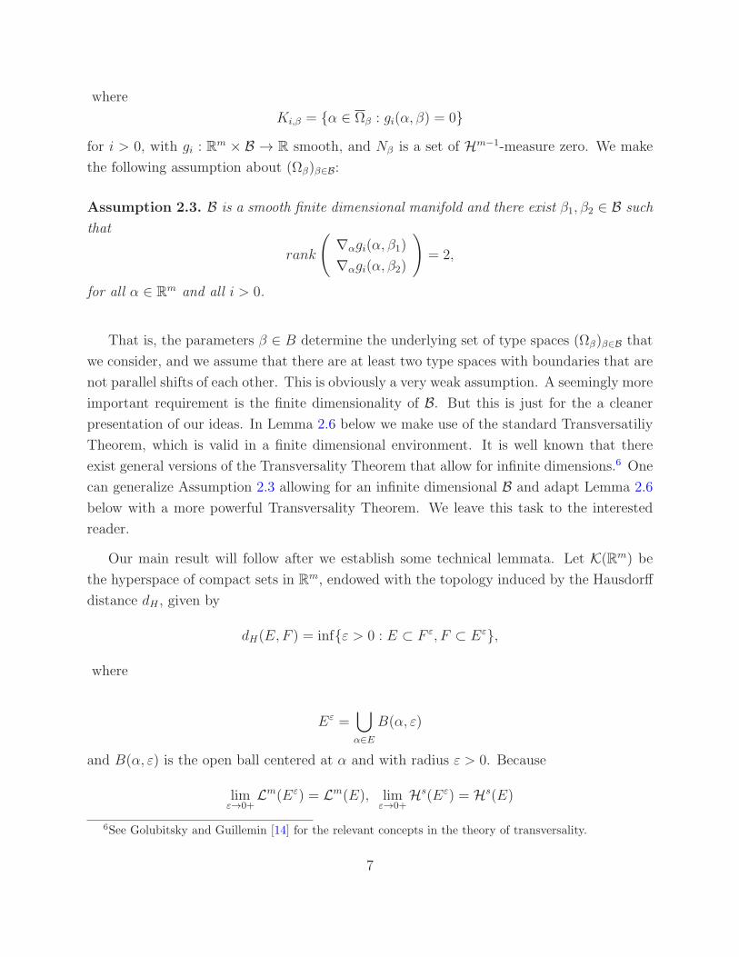
where

Ki,β = α ∈ Ωβ : gi(α, β) = 0

for i > 0, with gi : Rm × B → R smooth, and Nβ is a set of Hm−1-measure zero. We make

the following assumption about (Ωβ)β∈B:

Assumption 2.3. B is a smooth finite dimensional manifold and there exist β1, β2 ∈ B such

that

rank

(

∇αgi(α, β1)

∇αgi(α, β2)

)

= 2,

for all α ∈ Rm and all i > 0.

That is, the parameters β ∈ B determine the underlying set of type spaces (Ωβ)β∈B that

we consider, and we assume that there are at least two type spaces with boundaries that are

not parallel shifts of each other. This is obviously a very weak assumption. A seemingly more

important requirement is the finite dimensionality of B. But this is just for the a cleaner

presentation of our ideas. In Lemma 2.6 below we make use of the standard Transversatiliy

Theorem, which is valid in a finite dimensional environment. It is well known that there

exist general versions of the Transversality Theorem that allow for infinite dimensions.6 One

can generalize Assumption 2.3 allowing for an infinite dimensional B and adapt Lemma 2.6

below with a more powerful Transversality Theorem. We leave this task to the interested

reader.

Our main result will follow after we establish some technical lemmata. Let K(Rm) be

the hyperspace of compact sets in Rm, endowed with the topology induced by the Hausdorff

distance dH , given by

dH(E,F ) = infε > 0 : E ⊂ F ε, F ⊂ Eε,

where

Eε =⋃

α∈E

B(α, ε)

and B(α, ε) is the open ball centered at α and with radius ε > 0. Because

limε→0+

Lm(Eε) = Lm(E), limε→0+

Hs(Eε) = Hs(E)

6See Golubitsky and Guillemin [14] for the relevant concepts in the theory of transversality.

7

for all s ≥ 0, both Lm and Hs are upper semicontinuous functions in K(Rm) (Beer [9]).

Hence the following lemma holds.

Lemma 2.4. Let E ∈ K(Rm) be such that Lm(E) = Hs(E) = 0, for some s ≥ 0, and let

(Ek)k≥1 be a sequence in K(Rm) such that Ek → E. Then Lm(Ek) → 0 and Hs(Ek) → 0.

Proof. Because Lm is a non negative upper semicontinuous set function, we have

lim infEk→E

Lm(Ek) ≥ 0 = λ(E) ≥ lim supEk→E

Lm(Ek),

so Lm(Ek) → 0, and analogously for Hs.

Lemma 2.4 establishes continuity of Lebesgue and Hausdorff measures at zero. Let us

write Ω0,β = α ∈ Ωβ : s(α; β) = 0, where s(α; β) is the surplus function obtained by

type α when the underlying type space is Ωβ. Likewise, in what follows we make explicit the

dependence of the relevant object on the underlying type space indexed by β ∈ B. Extendings(·; β) by continuity on ∂Ωβ, let Ω0,β = α ∈ Ωβ : s(α; β) = 0.

Lemma 2.5. Under Assumption 2.1, Lm(Ω0,β) = 0 implies Ω0,β ⊂ ∂Ωβ.

Proof. If Ω0,β * ∂Ωβ, there is α ∈ Ω0,β and an ε > 0 with B(α, ε) ⊂ Ω. Then

Lm(α ∈ Ωβ : α ≤ α ∩ B(α, ε)) > 0.

Because of Assumption 2.1, we cannot have s(α; β) > 0 for any α ≤ α, for otherwise

s(α; β) > 0 as well. So

α ∈ Ωβ : α ≤ α ∩ B(α, ε) ⊂ Ω0,

contradicting Lm(Ω0,β) = 0.

Lemma 2.5 states that if the exclusion set has Lebesgue measure zero it should be part

of the topological boundary of the type set. Assumption 2.1 is crucial for this result. If it

does not hold it is easy to come up with counter-examples even in the one-dimensional case.

For examples, see Jullien [15].

Lemma 2.6. Assume Lm(Ω0,β) = 0 for all β in some open subset V ⊂ B, and that Assump-

tion 2.3 holds. Then Hm−1(Ω0,β) = 0 for an open and dense set of β ∈ V .

8

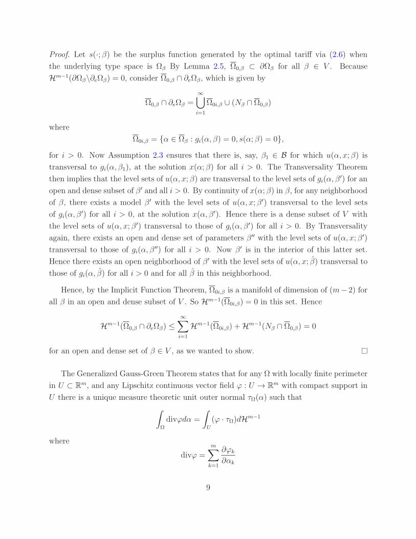
Proof. Let s(·; β) be the surplus function generated by the optimal tariff via (2.6) when

the underlying type space is Ωβ By Lemma 2.5, Ω0,β ⊂ ∂Ωβ for all β ∈ V . Because

Hm−1(∂Ωβ\∂eΩβ) = 0, consider Ω0,β ∩ ∂eΩβ, which is given by

Ω0,β ∩ ∂eΩβ =∞⋃

i=1

Ω0i,β ∪ (Nβ ∩ Ω0,β)

where

Ω0i,β = α ∈ Ωβ : gi(α, β) = 0, s(α; β) = 0,

for i > 0. Now Assumption 2.3 ensures that there is, say, β1 ∈ B for which u(α, x; β) is

transversal to gi(α, β1), at the solution x(α; β) for all i > 0. The Transversality Theorem

then implies that the level sets of u(α, x; β) are transversal to the level sets of gi(α, β′) for an

open and dense subset of β′ and all i > 0. By continuity of x(α; β) in β, for any neighborhood

of β, there exists a model β′ with the level sets of u(α, x; β′) transversal to the level sets

of gi(α, β′) for all i > 0, at the solution x(α, β′). Hence there is a dense subset of V with

the level sets of u(α, x; β′) transversal to those of gi(α, β′) for all i > 0. By Transversality

again, there exists an open and dense set of parameters β′′ with the level sets of u(α, x; β′)

transversal to those of gi(α, β′′) for all i > 0. Now β′ is in the interior of this latter set.

Hence there exists an open neighborhood of β′ with the level sets of u(α, x; β) transversal to

those of gi(α, β) for all i > 0 and for all β in this neighborhood.

Hence, by the Implicit Function Theorem, Ω0i,β is a manifold of dimension of (m− 2) for

all β in an open and dense subset of V . So Hm−1(Ω0i,β) = 0 in this set. Hence

Hm−1(Ω0,β ∩ ∂eΩβ) ≤∞∑

i=1

Hm−1(Ω0i,β) +Hm−1(Nβ ∩ Ω0,β) = 0

for an open and dense set of β ∈ V , as we wanted to show.

The Generalized Gauss-Green Theorem states that for any Ω with locally finite perimeter

in U ⊂ Rm, and any Lipschitz continuous vector field ϕ : U → Rm with compact support in

U there is a unique measure theoretic unit outer normal τΩ(α) such that

∫

Ω

divϕdα =

∫

U

(ϕ · τΩ)dHm−1

where

divϕ =m∑

k=1

∂ϕk

∂αk

9

is the divergence of the vector field ϕ.

The main result of this section is Theorem 2.7 below. It is stated without reference to

the well known sufficient conditions for implementability and differentiability of s(·) in order

to focus on the conditions that highlight the nature of the contribution being made.

Theorem 2.7. Consider the problem (2.2)-(2.3), and assume that it has a finite solution

yielding a continuous allocation x(α; β). Then, under Assumptions 2.1, 2.2 and 2.3, the set

of consumers with zero surplus at the solution has positive measure for almost all β ∈ B.

Proof. First we argue that, for each given β ∈ B, there is an equivalent metric in Rn for

which x(α; β), and hence s(α; β) and λ(α; β), are Lipschitz continuous functions (for a given

β ∈ B.) Let || · ||n and || · ||m be the Euclidean norms in Rn and Rm, respectively. Let

d1(α, α′) = ||α − α′||n + ||x(α; β) − x(α′; β)||m. Then ||x(α; β) − x(α′; β)||m < d1(α, α

′), so

x(·; β) is Lipschitz continuous. The metric d1 is equivalent to the Euclidean metric (Aliprantis

and Border [1], Lemma 3.12). Also, any Lipschitz continuous function under the Euclidean

metric in Rn (as the density f) is also Lipschitz continuous under d1. In fact, |f(α)−f(α′)| ≤c||α− α′||n = cd1(α, α

′)− c||x(α; β)− x(α′; β)||m ≤ cd1(α, α′), for some real number c.

Now, by way of contradiction, assume that Lm(Ω0,β) = 0 for all β in some open set

V ⊂ B. For any natural number k, let πk,β be the profit obtained by selling to the types in

Ωk,β = α ∈ Ωβ : s(α; β) ≤ 1

k.

Because c(·) is non-negative, we must have

πk,β ≤∫

Ωk,β

t(x(α; β))f(α)dα,

and from (2.5) we have

πk,β ≤∫

Ωk,β

u(α, x(α; β))f(α)dα.

Assumption 2.2 and the envelope condition (2.7) (with Lm(Ω0,β) = 0, we have Lm(Ωk,β) =

Lm(Ωk,β\Ω0,β), so the envelope condition holds for almost all types in Ωk,β) yield

πk,β ≤ K

∫

Ωk,β

(α · ∇s(α; β))λ(α; β)f(α)dα.

10

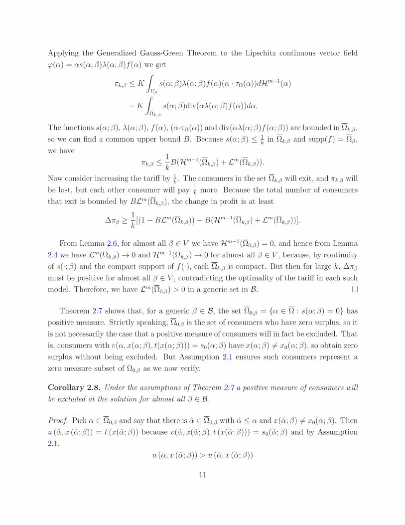
Applying the Generalized Gauss-Green Theorem to the Lipschitz continuous vector field

ϕ(α) = αs(α; β)λ(α; β)f(α) we get

πk,β ≤ K

∫

Uβ

s(α; β)λ(α; β)f(α)(α · τΩ(α))dHm−1(α)

−K

∫

Ωk,β

s(α; β)div(αλ(α; β)f(α))dα.

The functions s(α; β), λ(α; β), f(α), (α·τΩ(α)) and div(αλ(α; β)f(α; β)) are bounded in Ωk,β,

so we can find a common upper bound B. Because s(α; β) ≤ 1kin Ωk,β and supp(f) = Ωβ,

we have

πk,β ≤ 1

kB(Hm−1(Ωk,β) + Lm(Ωk,β)).

Now consider increasing the tariff by 1k. The consumers in the set Ωk,β will exit, and πk,β will

be lost, but each other consumer will pay 1kmore. Because the total number of consumers

that exit is bounded by BLm(Ωk,β), the change in profit is at least

∆πβ ≥ 1

k[(1− BLm(Ωk,β))− B(Hm−1(Ωk,β) + Lm(Ωk,β))].

From Lemma 2.6, for almost all β ∈ V we have Hm−1(Ω0,β) = 0, and hence from Lemma

2.4 we have Lm(Ωk,β) → 0 and Hm−1(Ωk,β) → 0 for almost all β ∈ V , because, by continuity

of s(·; β) and the compact support of f(·), each Ωk,β is compact. But then for large k, ∆πβ

must be positive for almost all β ∈ V , contradicting the optimality of the tariff in each such

model. Therefore, we have Lm(Ω0,β) > 0 in a generic set in B.

Theorem 2.7 shows that, for a generic β ∈ B, the set Ω0,β = α ∈ Ω : s(α; β) = 0 has

positive measure. Strictly speaking, Ω0,β is the set of consumers who have zero surplus, so it

is not necessarily the case that a positive measure of consumers will in fact be excluded. That

is, consumers with v(α, x(α; β), t(x(α; β))) = s0(α; β) have x(α; β) 6= x0(α; β), so obtain zero

surplus without being excluded. But Assumption 2.1 ensures such consumers represent a

zero measure subset of Ω0,β as we now verify.

Corollary 2.8. Under the assumptions of Theorem 2.7 a positive measure of consumers will

be excluded at the solution for almost all β ∈ B.

Proof. Pick α ∈ Ω0,β and say that there is α ∈ Ω0,β with α ≤ α and x(α; β) 6= x0(α; β). Then

u (α, x (α; β)) = t (x(α; β)) because v(α, x(α; β), t (x(α; β))) = s0(α; β) and by Assumption

2.1,

u (α, x (α; β)) > u (α, x (α; β))

11

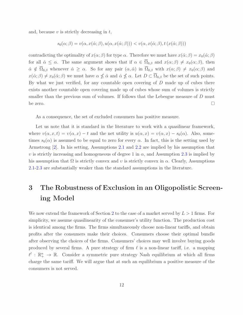
and, because v is strictly decreasing in t,

s0(α; β) = v(α, x(α; β), u(α, x(α; β))) < v(α, x(α; β), t (x(α; β)))

contradicting the optimality of x(α; β) for type α. Therefore we must have x(α; β) = x0(α; β)

for all α ≤ α. The same argument shows that if α ∈ Ω0,β and x(α; β) 6= x0(α; β), then

α /∈ Ω0,β whenever α ≥ α. So for any pair (α, α) in Ω0,β with x(α; β) 6= x0(α; β) and

x(α; β) 6= x0(α; β) we must have α α and α α. Let D ⊂ Ω0,β be the set of such points.

By what we just verified, for any countable open covering of D made up of cubes there

exists another countable open covering made up of cubes whose sum of volumes is strictly

smaller than the previous sum of volumes. If follows that the Lebesgue measure of D must

be zero.

As a consequence, the set of excluded consumers has positive measure.

Let us note that it is standard in the literature to work with a quasilinear framework,

where v(α, x, t) = υ(α, x) − t and the net utility is u(α, x) = υ(α, x) − s0(α). Also, some-

times s0(α) is assumed to be equal to zero for every α. In fact, this is the setting used by

Armstrong [2]. In his setting, Assumptions 2.1 and 2.2 are implied by his assumption that

υ is strictly increasing and homogeneous of degree 1 in α, and Assumption 2.3 is implied by

his assumption that Ω is strictly convex and υ is strictly convex in α. Clearly, Assumptions

2.1-2.3 are substantially weaker than the standard assumptions in the literature.

3 The Robustness of Exclusion in an Oligopolistic Screen-

ing Model

We now extend the framework of Section 2 to the case of a market served by L > 1 firms. For

simplicity, we assume quasilinearity of the consumer’s utility function. The production cost

is identical among the firms. The firms simultaneously choose non-linear tariffs, and obtain

profits after the consumers make their choices. Consumers choose their optimal bundle

after observing the choices of the firms. Consumers’ choices may well involve buying goods

produced by several firms. A pure strategy of firm ℓ is a non-linear tariff, i.e. a mapping

tℓ : Rn+ → R. Consider a symmetric pure strategy Nash equilibrium at which all firms

charge the same tariff. We will argue that at such an equilibrium a positive measure of the

consumers is not served.

12

Firm ℓ’s problem is to pick tℓ ∈ T ℓ, where T ℓ is the space of allowed tariffs, that solves

maxtℓ∈T ℓ

∫

Ω

(tℓ(xℓ(α))− c · xℓ(α))f(α)dα,

subject to:

x(α) ∈ argmaxx≥0 υ(α, x)− t(x) if maxx≥0 υ(α, x)− t(x) ≥ s0,ℓ (α)

x(α) = 0 otherwise

where

t(x) = min∑

j

tj(xj)

s.t.∑

j

xj = x, xj ≥ 0, (3.1)

and

s0,ℓ(α) = maxs∗0(α), maxx≥0,xℓ=0

(υ(α, x)− t−ℓ(x)) (3.2)

and t−ℓ(x) solves problem (3.1) subject to the additional constraint xℓ = 0. Equation

(3.2) states that the outside option of a consumer seen from the point of view of firm ℓ is

determined either by her best opportunity outside the market, s∗0(α), or by the best bundle

she may purchase from the competitors, maxx≥0,xℓ=0(υ(α, x)− t−ℓ(x)).

Define

u(α, xℓ) = υ(α, xℓ +∑

j 6=ℓ

xj(α))−∑

j 6=ℓ

tj(xj(α))− s0,ℓ(α),

where xj(α) is the equilibrium quantity purchased by the consumer of type α from firm j

and s0,ℓ(α) is given by (3.2). Then firm ℓ’s problem becomes:

maxtℓ∈T ℓ

∫

Ω

(tℓ(xℓ(α))− c · xℓ(α))f(α)dα,

subject to:

xℓ(α) ∈ argmaxx≥0 u(α, xℓ)− tℓ(xℓ) ifmaxx≥0 u(α, x

ℓ)− tℓ(xℓ) ≥ 0

xℓ(α) = 0 otherwise

Now u(α, xℓ) is endogenous and we cannot impose Assumptions 2.1 and 2.2 on it. Instead,

we use

Assumption 3.1. ∂2υ∂αi∂xj

> 0 for every i = 1, ...,m, j = 1, ..., n and x 6= x0(α).

13

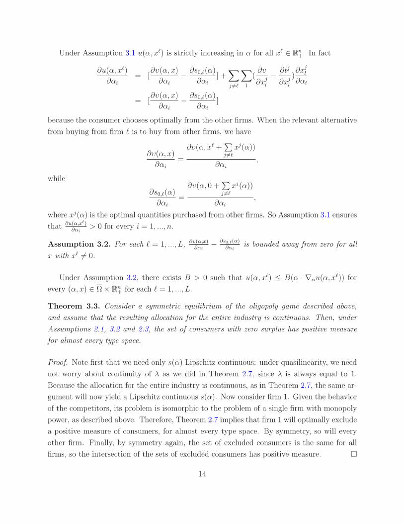
Under Assumption 3.1 u(α, xℓ) is strictly increasing in α for all xℓ ∈ Rn+. In fact

∂u(α, xℓ)

∂αi

= [∂υ(α, x)

∂αi

− ∂s0,ℓ(α)

∂αi

] +∑

j 6=ℓ

∑

l

(∂υ

∂xjl

− ∂tj

∂xjl

)∂xj

l

∂αi

= [∂υ(α, x)

∂αi

− ∂s0,ℓ(α)

∂αi

]

because the consumer chooses optimally from the other firms. When the relevant alternative

from buying from firm ℓ is to buy from other firms, we have

∂υ(α, x)

∂αi

=

∂υ(α, xℓ +∑

j 6=ℓ

xj(α))

∂αi

,

while

∂s0,ℓ(α)

∂αi

=

∂υ(α, 0 +∑

j 6=ℓ

xj(α))

∂αi

,

where xj(α) is the optimal quantities purchased from other firms. So Assumption 3.1 ensures

that ∂u(α,xℓ)∂αi

> 0 for every i = 1, ..., n.

Assumption 3.2. For each ℓ = 1, ..., L, ∂υ(α,x)∂αi

− ∂s0,ℓ(α)

∂αiis bounded away from zero for all

x with xℓ 6= 0.

Under Assumption 3.2, there exists B > 0 such that u(α, xℓ) ≤ B(α · ∇αu(α, xℓ)) for

every (α, x) ∈ Ω× Rn+ for each ℓ = 1, ..., L.

Theorem 3.3. Consider a symmetric equilibrium of the oligopoly game described above,

and assume that the resulting allocation for the entire industry is continuous. Then, under

Assumptions 2.1, 3.2 and 2.3, the set of consumers with zero surplus has positive measure

for almost every type space.

Proof. Note first that we need only s(α) Lipschitz continuous: under quasilinearity, we need

not worry about continuity of λ as we did in Theorem 2.7, since λ is always equal to 1.

Because the allocation for the entire industry is continuous, as in Theorem 2.7, the same ar-

gument will now yield a Lipschitz continuous s(α). Now consider firm 1. Given the behavior

of the competitors, its problem is isomorphic to the problem of a single firm with monopoly

power, as described above. Therefore, Theorem 2.7 implies that firm 1 will optimally exclude

a positive measure of consumers, for almost every type space. By symmetry, so will every

other firm. Finally, by symmetry again, the set of excluded consumers is the same for all

firms, so the intersection of the sets of excluded consumers has positive measure.

14

Observe that the kind of competition in nonlinear tariffs described above is not necessarily

of the undercutting nature of Bertrand price competition. For instance, say that two firms

offer the same tariff, and that a type α optimally buys half of her bundle from each firm

(because the cost of the total bundle is larger than two times the cost of half of the bundle).

Then one firm can increase its profits by charging a bit more for half of the bundle, in such

a way that the consumer, while buying a larger fraction from the other firm, will still buy

close to half of the bundle from the given firm, but the cost of that smaller fraction may well

be significantly smaller than the cost of half of the bundle. If competition was simply done

by undercutting, then the result in Theorem 3.3 would not be valid, for firms would always

want to serve the entire market.

Let us now assume that the number of producers is not fixed but there is a positive entry

cost F > 0. It is easy to see that this problem can be reduced to the previous one, since

equilibrium number of the producers is always finite. Indeed, with K producers the profits of

an oligopolist in a symmetric equilibrium are bounded by πm/K, where πm are the profits of

a monopolist. Therefore, at equilibrium K ≤ πm/F and a positive measure of the consumers

will be excluded from the market.

3.1 Existence of Equilibrium in the Oligopolgy Game

Theorem 3.3 is derived under the assumption that a symmetric Nash equilibrium exists for

the game played by the firms. Champsuar and Rochet [10] note that the profit functions of

the firms might be discontinuous when there are bunching regions. Even though Basov [7]

shows that bunching in the multidimensional case is not as typical as suggested by Rochet

and Chone [21], existence of an equilibrium has to be established. That’s what we do next.

Assume that the space T of allowed tariffs is the space of all bounded monotonic functions

from X to [0,M ], where X ⊂ Rn+ is a compact subset of feasible bundles and M is a bound

on the net utility function, hence it is also a bound on the tariffs. The space T is the common

strategy space of each producer ℓ = 1, ..., L. By Helly’s theorem, every sequence of tariffs in

T has a pointwise convergent subsequence, so T is compact in the topology of a.e. pointwise

convergence (where a.e. refers to the Lebesgue measure Lm.) Let ∆(T ) denote the space

of Borel probability measures on T , endowed with the weak* topology, so it is a compact,

convex space.

Assume that when firms choose a symmetric profile (t, ..., t) of tariffs, they obtain the

15

same expected profit: πℓ(t, ..., t) = π(t, ..., t) for ℓ = 1, ..., L.7 Hence the one-shot game

(T × · · · × T, π, ..., π) played by the firms is symmetric, and so is its mixed extension, where

firms choose σ ∈ ∆(T ) and payoffs are extended to mixtures by taking expectations. For ease

of notation, let (σ, σ) denote the profile (σ, ..., σ, ..., σ) of strategies where one firm chooses

σ and the others all choose σ. Use π(σ, σ) to denote the expected profit of the firm choosing

σ.

Proposition 3.4. The compact, convex and symmetric game described above has a symmet-

ric mixed strategy Nash equilibrium.

Proof. We show that the game is diagonally better reply secure (Reny [19]). Let (σ, σ) be

a non equilibrium profile, and consider π∗ = lim π(σn, σn) for some sequence with σn → σ.

For any ε > 0, there exists a strictly increasing tε with π(tε, σ) > π(σ, σ), as (σ, σ) is not an

equilibrium. Because tε is strictly increasing, π(tε, ·) is continuous at σ. If π∗ = π(σ, σ), then

diagonal better reply security is verified. If not, then we have discontinuities at (σ, σ). Along

any sequence σn converging to σ, there is at least one firm whose profit drops at the limit,

and this firm can obtain a profit strictly higher than π∗ by using tε instead of σn, for large

n. Hence diagonal better reply security is again verified due to continuity of π(tε, ·).

Observe that Theorem 3.3 remains valid at a symmetric mixed strategy equilibrium. As

long as the surplus function is Lipschitz continuous, the formulation of the oligopoly game

allows us to ascertain that a small increase in every t in the support of σ will be profitable

if the measure of excluded types is not positive.

4 Examples and Applications

Let us begin with some examples illustrating Assumptions 2.1, 2.2 and 2.3.

Example 4.1. Consider a consumer who lives for two periods. Her wealth in the first

period is w and in the second period her wealth can take two values, wH or wL. Let p be

the probability that w = wH , and let δ ∈ (0, 1) be the discount factor, so that the private

information of the consumer is characterized by a two-dimensional vector α = (1− p, 1− δ).

7Either because the consumer chooses optimally to buy a fraction 1

Lof the optimal bundle from each

firm, or because she visits each firm with probability 1

L, depending on the shape of the commonly offered

non-linear tariff t.

16

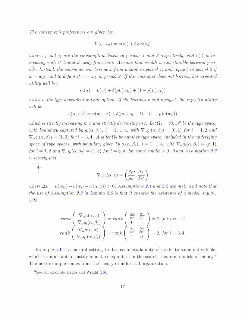
The consumer’s preferences are given by:

V (c1, c2) = υ(c1) + δEυ(c2)

where c1 and c2 are the consumption levels in periods 1 and 2 respectively, and υ(·) is in-

creasing with υ′ bounded away from zero. Assume that wealth is not storable between peri-

ods. Instead, the consumer can borrow x from a bank in period 1, and repay t in period 2 if

w = wH , and to defaut if w = wL in period 2. If the consumer does not borrow, her expected

utility will be:

s0(α) = υ(w) + δ(pυ(wH) + (1− p)υ(wL))

which is the type dependent outside option. If she borrows x and repays t, the expected utility

will be

v(α, x, t) = υ(w + x) + δ(pυ(wH − t) + (1− p)υ(wL))

which is strictly increasing in x and strictly decreasing in t. Let Ω1 = (0, 1)2 be the type space,

with boundary captured by gi(α, β1), i = 1, ..., 4, with ∇αgi(α, β1) = (0, 1) for i = 1, 2 and

∇αgi(α, β1) = (1, 0) for i = 3, 4. And let Ω2 be another type space, included in the underlying

space of type spaces, with boundary given by gi(α, β2), i = 1, ..., 4, with ∇αgi(α, β2) = (ε, 1)

for i = 1, 2 and ∇αgi(α, β2) = (1, ε) for i = 3, 4, for some smallε > 0. Then Assumption 2.3

is clearly met.

As

∇αu (α, x) =

(

∆υ

pυ′,∆υ

δυ′

)

where ∆υ = υ(wH)−υ(wH −u (α, x)) > 0, Assumptions 2.1 and 2.2 are met. And note that

the use of Assumption 2.3 in Lemma 2.6 is that it ensures the existence of a model, say β1,

with

rank

(

∇αu(α, x)

∇αgi(α, β1)

)

= rank

(

∆υpυ′

∆υδυ′

0 1

)

= 2, for i = 1, 2

rank

(

∇αu(α, x)

∇αgj(α, β1)

)

= rank

(

∆υpυ′

∆υδυ′

1 0

)

= 2, for i = 3, 4.

Example 4.1 is a natural setting to discuss unavailability of credit to some individuals,

which is important to justify monetary equilibria in the search theoretic models of money.8

The next example comes from the theory of industrial organization.

8See, for example, Lagos and Wright [16].

17

Example 4.2. Suppose a monopolist produces cars of high quality. The utility of a consumer

is quasilinear, v(α, x, t) = υ(α, x)− t, with

υ(α, x) = A+n∑

i=1

αixi (4.1)

where A > 0 can be interpreted as utility of driving a car, and the second term in (4.1) is a

quality premium. Suppose a consumer has three choices: to buy a car from the monopolist,

to buy a car from a competitive fringe, and to buy no car at all. We will normalize the utility

of buying no car at all to be zero. Assume the competitive fringe serves cars of quality −x0,

where x0 ∈ Rn++ at price p. That is, the consumers experience disutility from the quality of

the cars of the competitive fringe, and the higher their type, the higher the disutility. The

utility of the outside option in this case is given by:

s0(α) = max(0, A− p−n∑

i=1

αix0i)

and is decreasing in α. Therefore, Assumptions 2.1 and 2.2 hold, because in a quasilinear

setting the net utility is u(α, x) = υ(α, x)− s0(α). As for Assumption 2.3, say that we start

off with Ω being the unit square in Rn. Parametrize each of the edges, and consider models

obtained by small perturbations of the parameters, hence the edges (like for instance small

rotations of the unit square). When such type spaces are included in B, Assumption 2.3 is

met.

Now let us turn to models that do not satisfy Assumptions 2.1, 2.2 and 2.3. First,

consider any model that yields an excluded set Ω0 with positive measure, and modify the

problem considering only the types in Ω\Ω′, where Ω0 ⊂ Ω′. Would the modified problem

have no exclusion? Though this will indeed be the case if Ω′ = Ω0,9 it will not hold for a

generic superset Ω′. This would only be the case if the shape of Ω0 stood in a tight relation

with the shape of Ω′, a non generic situation. That is, even if Ω0 stood in the particular

tight relation with Ω′, a slight change in the boundary structure of Ω′ would suffice for us to

have exclusion in the modified model.

In the same vein, Rochet and Stole [23] provided an example where the exclusion set is

empty.10 In their quasilinear example υ : Ω×R+ → R has the form

υ(α, x) = (α1 + α2)x

9We are grateful to an anonymous referee for this observation.10Another example along similar lines is provided by Deneckere and Severinov [12]. Though it is a bit

more intricate and the authors provide sufficient conditions that ensure full participation in the case of one

quality dimension and two-dimensional characteristics, their condition also does not hold generically.

18

and Ω is a rectangle with sides parallel to the 45 degrees and −45 degrees lines. They argued

that one can shift the rectangle sufficiently far to the right to have an empty exclusion region.

Their result is driven by the fact that they allow only very special collection of type spaces,

rectangles with parallel sides. Formally, the model used in this case cannot be used in Lemma

2.6 because ∇αgi(α, β) = (1, 1) for i = 1, 3 and ∇αgi(α, β) = (−1, 1) for i = 2, 4, so that

(using u(α, x) = υ(α, x) because s0(α) = 0)

(

∇αu(α, x)

∇αgi(α, β)

)

=

(

x x

1 1

)

⇒ rank

(

∇αu(α, x)

∇αgi(α, β)

)

= 1

for i = 1, 3.

Observe that a very small change in the type set changes that result. Consider, for

example, a slightly perturbed type space, with ∇αgi(α, β0) = (1, 1 + ε), for i = 1, 3, where ε

is a small positive real number. Then, for all x 6= 0 and i = 1, ..., 4

rank

(

∇αu(α, x)

∇αgi(α, β0)

)

= 2

as required in Lemma 2.6.

We stress that our result does not guarantee a non-empty exclusion region for every

multi-dimensional screening problem. Rather, it asserts that problems for which the ex-

clusion region is empty can be slightly perturbed and transformed into problems with a

positive measure of excluded consumers. To understand the results intuitively, assume first

that, in equilibrium, all consumers are served. First, note that at least one consumer should

be indifferent between participating and not participating, since otherwise the tariffs can

be uniformly increased for everyone by a small amount, increasing the monopolist’s profits.

Now, consider increasing the tariff by ε > 0. The consumers who used to obtain surplus

below ε will drop out. The measure of such consumers is o(ε), unless the iso-surplus hyper-

surfaces happen to be parallel to the boundary of the type space. Under Assumption 2.3,

there will be a model where the iso-surplus hyper-surfaces will not only not be parallel to

the boundary of Ω, it will be transversal. Such situations may still occur endogenously,

which is the reason why our result holds for almost all, rather then for all, screening prob-

lems. One class of problems, for which full participation may occur are models with random

outside options. They were first considered by Rochet and Stole [22] for both monopolistic

and oligopolistic settings and generalized by Basov and Yin [8] for the case of risk averse

principal(s). Armstrong and Vickers [5] considered another generalization, allowing for mul-

tidimensional vertical types. In this type of models, the type consists of a vector of vertical

19

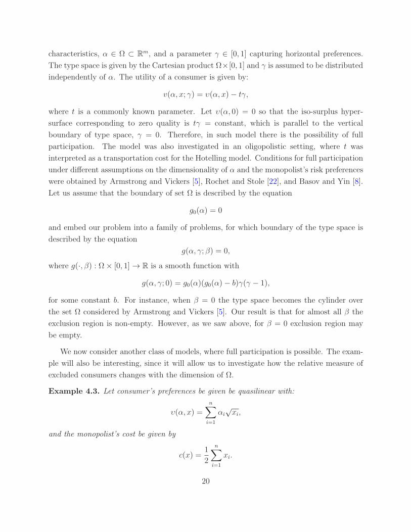
characteristics, α ∈ Ω ⊂ Rm, and a parameter γ ∈ [0, 1] capturing horizontal preferences.

The type space is given by the Cartesian product Ω×[0, 1] and γ is assumed to be distributed

independently of α. The utility of a consumer is given by:

v(α, x; γ) = υ(α, x)− tγ,

where t is a commonly known parameter. Let υ(α, 0) = 0 so that the iso-surplus hyper-

surface corresponding to zero quality is tγ = constant, which is parallel to the vertical

boundary of type space, γ = 0. Therefore, in such model there is the possibility of full

participation. The model was also investigated in an oligopolistic setting, where t was

interpreted as a transportation cost for the Hotelling model. Conditions for full participation

under different assumptions on the dimensionality of α and the monopolist’s risk preferences

were obtained by Armstrong and Vickers [5], Rochet and Stole [22], and Basov and Yin [8].

Let us assume that the boundary of set Ω is described by the equation

g0(α) = 0

and embed our problem into a family of problems, for which boundary of the type space is

described by the equation

g(α, γ; β) = 0,

where g(·, β) : Ω× [0, 1] → R is a smooth function with

g(α, γ; 0) = g0(α)(g0(α)− b)γ(γ − 1),

for some constant b. For instance, when β = 0 the type space becomes the cylinder over

the set Ω considered by Armstrong and Vickers [5]. Our result is that for almost all β the

exclusion region is non-empty. However, as we saw above, for β = 0 exclusion region may

be empty.

We now consider another class of models, where full participation is possible. The exam-

ple will also be interesting, since it will allow us to investigate how the relative measure of

excluded consumers changes with the dimension of Ω.

Example 4.3. Let consumer’s preferences be given be quasilinear with:

υ(α, x) =n∑

i=1

αi

√xi,

and the monopolist’s cost be given by

c(x) =1

2

n∑

i=1

xi.

20

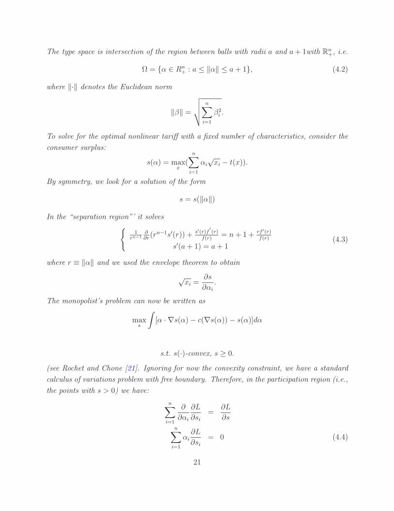
The type space is intersection of the region between balls with radii a and a+ 1with Rn+, i.e.

Ω = α ∈ Rn+ : a ≤ ‖α‖ ≤ a+ 1, (4.2)

where ‖·‖ denotes the Euclidean norm

‖β‖ =

√

√

√

√

n∑

i=1

β2i .

To solve for the optimal nonlinear tariff with a fixed number of characteristics, consider the

consumer surplus:

s(α) = maxx

(n∑

i=1

αi

√xi − t(x)).

By symmetry, we look for a solution of the form

s = s(‖α‖)

In the “separation region”’ it solves

1rn−1

∂∂r(rn−1s′(r)) + s′(r)f

′

(r)f(r)

= n+ 1 + rf ′(r)f(r)

s′(a+ 1) = a+ 1(4.3)

where r ≡ ‖α‖ and we used the envelope theorem to obtain

√xi =

∂s

∂αi

.

The monopolist’s problem can now be written as

maxs

∫

[α · ∇s(α)− c(∇s(α))− s(α)]dα

s.t. s(·)-convex, s ≥ 0.

(see Rochet and Chone [21]. Ignoring for now the convexity constraint, we have a standard

calculus of variations problem with free boundary. Therefore, in the participation region (i.e.,

the points with s > 0) we have:

n∑

i=1

∂

∂αi

∂L

∂si=

∂L

∂s

n∑

i=1

αi

∂L

∂si= 0 (4.4)

21

(see Basov [7]), where si denotes the ith partial derivative of s and

L = α · ∇s(α)− c(∇s(α))− s(α)

Observe that this is exactly the system (4.3). Assume that types are distributed uniformly on

Ω, so the derivative of the type distribution vanishes. Then, solving (4.3) we get:

xi(α) = [max(0,αi

n(n+ 1− (

a+ 1

r)n))]2.

The corresponding iso-surplus hyper-surfaces are given by the intersection of a sphere of

appropriate dimension with Rn+. They are parallel to the boundary, hence it is possible that

the exclusion region is empty. Note that the exclusion region is given by

Ω0 = α ∈ Ω : ‖α‖ ≤ a+ 1n√1 + n

,

so it is non-empty ifa+ 1n√1 + n

> a.

Observe that if n = 1 the exclusion region is empty if and only if a > 1, if n = 2 it is empty

if and only if a > 1/(√3− 1) ≈ 1.36, and since

limn→∞

1n√1 + n

= 1,

the exclusion region is non-empty for any a > 0 for sufficiently large n. The relative measure

of the excluded consumer’s (the measure of excluded consumers if we normalize the total

measure of consumers to be one for all n) is:

ζ =(a+ 1)n/(n+ 1)− an

(a+ 1)n − an.

It is easy to see that as n → ∞ the measure of excluded consumers converges to zero as

1/n goes to zero, i.e. as exclusion becomes asymptotically less important. This accords with

results obtained by Armstrong [3]. The convergence, however, is not monotone. For example,

if a = 1.3 the measure of excluded customers first rises from zero for n = 1 to 11.6% for

n = 5, and falls slowly thereafter. For a = 2 maximal exclusion of 8.3% obtains when n = 11

and for a = 0.7 maximal exclusion of 19.7% obtains when n = 2.

Also observe that, although an asymptotically higher fraction of consumers gets served as

n → ∞, this does not mean that the consumers become better off. Indeed, as n → ∞ the

radius of the exclusion region converges to (a+ 1). That is, almost all served consumers are

located near the upper boundary. This means that the trade-off between the efficient provision

of quality and minimization of information rents disappears. Asymptotically, the monopolist

provides the efficient quality but is able to appropriate almost the entire surplus.

22

4.1 An Application to the Regulation of a Monopolist with Un-

known Demand and Cost Functions

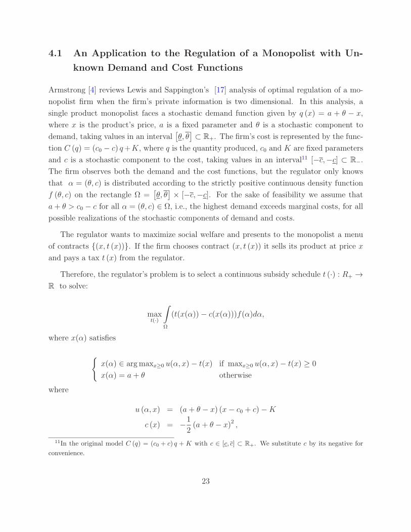
Armstrong [4] reviews Lewis and Sappington’s [17] analysis of optimal regulation of a mo-

nopolist firm when the firm’s private information is two dimensional. In this analysis, a

single product monopolist faces a stochastic demand function given by q (x) = a + θ − x,

where x is the product’s price, a is a fixed parameter and θ is a stochastic component to

demand, taking values in an interval[

θ, θ]

⊂ R+. The firm’s cost is represented by the func-

tion C (q) = (c0 − c) q+K, where q is the quantity produced, c0 and K are fixed parameters

and c is a stochastic component to the cost, taking values in an interval11 [−c,−c] ⊂ R−.

The firm observes both the demand and the cost functions, but the regulator only knows

that α = (θ, c) is distributed according to the strictly positive continuous density function

f (θ, c) on the rectangle Ω =[

θ, θ]

× [−c,−c]. For the sake of feasibility we assume that

a+ θ > c0 − c for all α = (θ, c) ∈ Ω, i.e., the highest demand exceeds marginal costs, for all

possible realizations of the stochastic components of demand and costs.

The regulator wants to maximize social welfare and presents to the monopolist a menu

of contracts (x, t (x)). If the firm chooses contract (x, t (x)) it sells its product at price x

and pays a tax t (x) from the regulator.

Therefore, the regulator’s problem is to select a continuous subsidy schedule t (·) : R+ →R to solve:

maxt(·)

∫

Ω

(t(x(α))− c(x(α)))f(α)dα,

where x(α) satisfies

x(α) ∈ argmaxx≥0 u(α, x)− t(x) if maxx≥0 u(α, x)− t(x) ≥ 0

x(α) = a+ θ otherwise

where

u (α, x) = (a+ θ − x) (x− c0 + c)−K

c (x) = −1

2(a+ θ − x)2 ,

11In the original model C (q) = (c0 + c) q + K with c ∈ [c, c] ⊂ R+. We substitute c by its negative for

convenience.

23

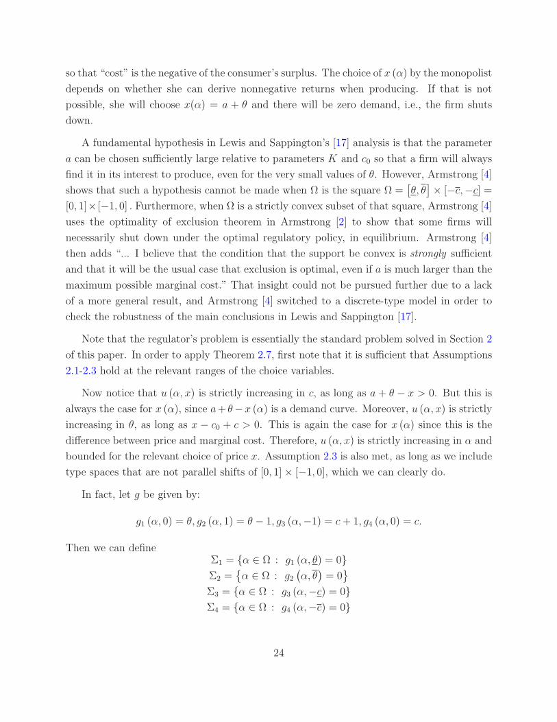
so that “cost” is the negative of the consumer’s surplus. The choice of x (α) by the monopolist

depends on whether she can derive nonnegative returns when producing. If that is not

possible, she will choose x(α) = a + θ and there will be zero demand, i.e., the firm shuts

down.

A fundamental hypothesis in Lewis and Sappington’s [17] analysis is that the parameter

a can be chosen sufficiently large relative to parameters K and c0 so that a firm will always

find it in its interest to produce, even for the very small values of θ. However, Armstrong [4]

shows that such a hypothesis cannot be made when Ω is the square Ω =[

θ, θ]

× [−c,−c] =

[0, 1]× [−1, 0] . Furthermore, when Ω is a strictly convex subset of that square, Armstrong [4]

uses the optimality of exclusion theorem in Armstrong [2] to show that some firms will

necessarily shut down under the optimal regulatory policy, in equilibrium. Armstrong [4]

then adds “... I believe that the condition that the support be convex is strongly sufficient

and that it will be the usual case that exclusion is optimal, even if a is much larger than the

maximum possible marginal cost.” That insight could not be pursued further due to a lack

of a more general result, and Armstrong [4] switched to a discrete-type model in order to

check the robustness of the main conclusions in Lewis and Sappington [17].

Note that the regulator’s problem is essentially the standard problem solved in Section 2

of this paper. In order to apply Theorem 2.7, first note that it is sufficient that Assumptions

2.1-2.3 hold at the relevant ranges of the choice variables.

Now notice that u (α, x) is strictly increasing in c, as long as a + θ − x > 0. But this is

always the case for x (α), since a+ θ−x (α) is a demand curve. Moreover, u (α, x) is strictly

increasing in θ, as long as x − c0 + c > 0. This is again the case for x (α) since this is the

difference between price and marginal cost. Therefore, u (α, x) is strictly increasing in α and

bounded for the relevant choice of price x. Assumption 2.3 is also met, as long as we include

type spaces that are not parallel shifts of [0, 1]× [−1, 0], which we can clearly do.

In fact, let g be given by:

g1 (α, 0) = θ, g2 (α, 1) = θ − 1, g3 (α,−1) = c+ 1, g4 (α, 0) = c.

Then we can defineΣ1 = α ∈ Ω : g1 (α, θ) = 0Σ2 =

α ∈ Ω : g2(

α, θ)

= 0

Σ3 = α ∈ Ω : g3 (α,−c) = 0Σ4 = α ∈ Ω : g4 (α,−c) = 0

24

Therefore, the boundary of Ω can be expressed as:

∂Ω =4∪i=1

Σi.

Moreover, the gradient of function u is

∇αu(α, x) = (x− c0 + c, a+ θ − x)

and

∇αgi(α, β) = (1, 0) , i = 1, 2,∇αgj(α, β) = (0, 1) , j = 1, 2.

Therefore, for i = 1, 2 and for j = 1, 2,

(

∇αu(α, x)

∇αgi(α, β)

)

=

(

x− c0 + c a+ θ − x

1 0

)

(

∇αu(α, x)

∇αgj(α, β)

)

=

(

x− c0 + c a+ θ − x

0 1

)

In particular, the rank of these matrices is 2, and we illustrate once again the use of

Assumption 2.3 in Lemma 2.6.12 All the hypothesis of Theorem 2.7 are satisfied, so we may

conclude that a set of positive firms will generically be excluded from the regulated market,

i.e., will not produce at all. Armstrong’s [4] conjecture is therefore confirmed.

4.2 An Application to Involuntary Unemployment

Consider a firm in an industry that produces n goods captured by a vector x ∈ Rn+. The

firm hires workers to produce these goods. A worker is characterized by the cost she bears

in order to produce goods x ∈ Rn+, which is given by the effort cost function e (α, x). The

parameter α ∈ Ω ⊂ Rm is the worker’s unobservable type distributed on an open, bounded,

set Ω ⊂ Rm according to a strictly positive, continuous density function f(·).

Therefore, if a worker of type α is hired to produce output x and receives wage ω (x),

her utility is ω (x)− e (α, x) , where c(α, ·) is cost of effort, which depends on the type of the

worker. If the worker is not hired by the firm, she will receive a net utility s0 (α), either by

working on a different firm, or by receiving unemployment compensation.

12Indeed, it cannot be the case that x = p = c0 − c = a + θ since the price cannot be, at the same time,

the marginal cost (prefect competitive price) and the price that makes demand vanish.

25

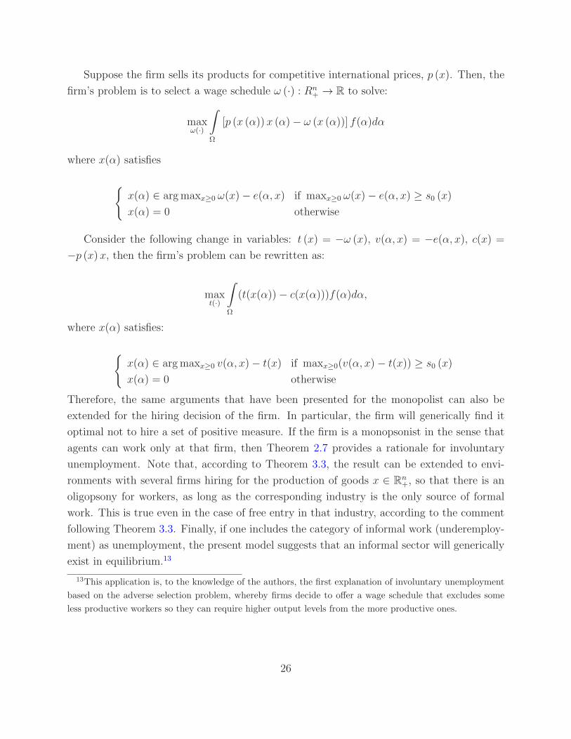
Suppose the firm sells its products for competitive international prices, p (x). Then, the

firm’s problem is to select a wage schedule ω (·) : Rn+ → R to solve:

maxω(·)

∫

Ω

[p (x (α)) x (α)− ω (x (α))] f(α)dα

where x(α) satisfies

x(α) ∈ argmaxx≥0 ω(x)− e(α, x) if maxx≥0 ω(x)− e(α, x) ≥ s0 (x)

x(α) = 0 otherwise

Consider the following change in variables: t (x) = −ω (x), v(α, x) = −e(α, x), c(x) =

−p (x) x, then the firm’s problem can be rewritten as:

maxt(·)

∫

Ω

(t(x(α))− c(x(α)))f(α)dα,

where x(α) satisfies:

x(α) ∈ argmaxx≥0 v(α, x)− t(x) if maxx≥0(v(α, x)− t(x)) ≥ s0 (x)

x(α) = 0 otherwise

Therefore, the same arguments that have been presented for the monopolist can also be

extended for the hiring decision of the firm. In particular, the firm will generically find it

optimal not to hire a set of positive measure. If the firm is a monopsonist in the sense that

agents can work only at that firm, then Theorem 2.7 provides a rationale for involuntary

unemployment. Note that, according to Theorem 3.3, the result can be extended to envi-

ronments with several firms hiring for the production of goods x ∈ Rn+, so that there is an

oligopsony for workers, as long as the corresponding industry is the only source of formal

work. This is true even in the case of free entry in that industry, according to the comment

following Theorem 3.3. Finally, if one includes the category of informal work (underemploy-

ment) as unemployment, the present model suggests that an informal sector will generically

exist in equilibrium.13

13This application is, to the knowledge of the authors, the first explanation of involuntary unemployment

based on the adverse selection problem, whereby firms decide to offer a wage schedule that excludes some

less productive workers so they can require higher output levels from the more productive ones.

26

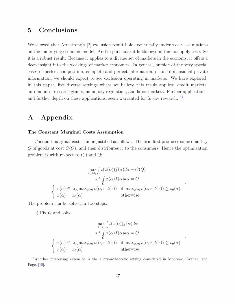
5 Conclusions

We showed that Armstrong’s [2] exclusion result holds generically under weak assumptions

on the underlying economic model. And in particular it holds beyond the monopoly case. So

it is a robust result. Because it applies to a diverse set of markets in the economy, it offers a

deep insight into the workings of market economies. In general, outside of the very special

cases of perfect competition, complete and perfect information, or one-dimensional private

information, we should expect to see exclusion operating in markets. We have explored,

in this paper, five diverse settings where we believe this result applies: credit markets,

automobiles, research grants, monopoly regulation, and labor markets. Further applications,

and further depth on these applications, seem warranted for future research. 14

A Appendix

The Constant Marginal Costs Assumption

Constant marginal costs can be justified as follows. The firm first produces some quantity

Q of goods at cost C(Q), and then distributes it to the consumers. Hence the optimization

problem is with respect to t(·) and Q:

maxt(·),Q

∫

Ω

t(x(α))f(α)dα− C(Q)

s.t.∫

Ω

x(α)f(α)dα = Q

x(α) ∈ argmaxx≥0 v(α, x, t(x)) if maxx≥0 v(α, x, t(x)) ≥ s0(α)

x(α) = x0(α) otherwise.

.

The problem can be solved in two steps:

a) Fix Q and solve

maxt(·)

∫

Ω

t(x(α))f(α)dα

s.t.∫

Ω

x(α)f(α)dα = Q

x(α) ∈ argmaxx≥0 v(α, x, t(x)) if maxx≥0 v(α, x, t(x)) ≥ s0(α)

x(α) = x0(α) otherwise.

.

14Another interesting extension is the auction-theoretic setting considered in Monteiro, Svaiter, and

Page, [18].

27

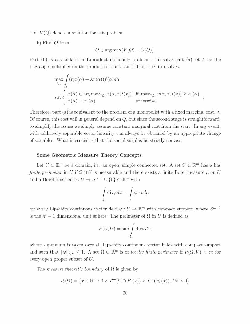
Let V (Q) denote a solution for this problem.

b) Find Q from

Q ∈ argmax(V (Q)− C(Q)).

Part (b) is a standard multiproduct monopoly problem. To solve part (a) let λ be the

Lagrange multiplier on the production constraint. Then the firm solves:

maxt(·)

∫

Ω

(t(x(α)− λx(α))f(α)dα

s.t.

x(α) ∈ argmaxx≥0 v(α, x, t(x)) if maxx≥0 v(α, x, t(x)) ≥ s0(α)

x(α) = x0(α) otherwise..

Therefore, part (a) is equivalent to the problem of a monopolist with a fixed marginal cost, λ.

Of course, this cost will in general depend on Q, but since the second stage is straightforward,

to simplify the issues we simply assume constant marginal cost from the start. In any event,

with additively separable costs, linearity can always be obtained by an appropriate change

of variables. What is crucial is that the social surplus be strictly convex.

Some Geometric Measure Theory Concepts

Let U ⊂ Rm be a domain, i.e. an open, simple connected set. A set Ω ⊂ Rm has a has

finite perimeter in U if Ω ∩ U is measurable and there exists a finite Borel measure µ on U

and a Borel function v : U → Sm−1 ∪ 0 ⊂ Rm with

∫

Ω

divϕdx =

∫

U

ϕ · vdµ

for every Lipschitz continuous vector field ϕ : U → Rm with compact support, where Sm−1

is the m− 1 dimensional unit sphere. The perimeter of Ω in U is defined as:

P (Ω, U) = sup

∫

U

divϕdx,

where supremum is taken over all Lipschitz continuous vector fields with compact support

and such that ‖ϕ‖L∞ ≤ 1. A set Ω ⊂ Rm is of locally finite perimeter if P (Ω, V ) < ∞ for

every open proper subset of U .

The measure theoretic boundary of Ω is given by

∂e(Ω) = x ∈ Rm : 0 < Lm(Ω ∩ Bε(x)) < Lm(Bε(x)), ∀ε > 0

28

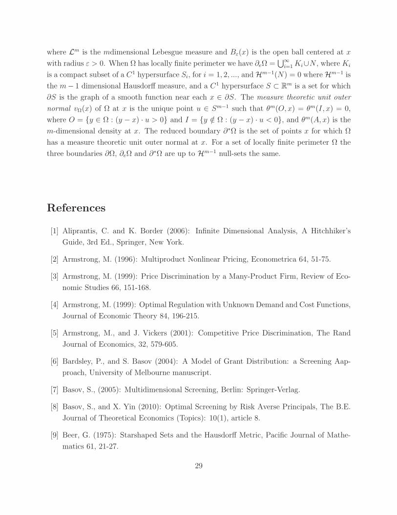
where Lm is the mdimensional Lebesgue measure and Bε(x) is the open ball centered at x

with radius ε > 0. When Ω has locally finite perimeter we have ∂eΩ =⋃∞

i=1 Ki∪N , where Ki

is a compact subset of a C1 hypersurface Si, for i = 1, 2, ..., and Hm−1(N) = 0 where Hm−1 is

the m− 1 dimensional Hausdorff measure, and a C1 hypersurface S ⊂ Rm is a set for which

∂S is the graph of a smooth function near each x ∈ ∂S. The measure theoretic unit outer

normal vΩ(x) of Ω at x is the unique point u ∈ Sm−1 such that θm(O, x) = θm(I, x) = 0,

where O = y ∈ Ω : (y − x) · u > 0 and I = y /∈ Ω : (y − x) · u < 0, and θm(A, x) is the

m-dimensional density at x. The reduced boundary ∂∗Ω is the set of points x for which Ω

has a measure theoretic unit outer normal at x. For a set of locally finite perimeter Ω the

three boundaries ∂Ω, ∂eΩ and ∂∗Ω are up to Hm−1 null-sets the same.

References

[1] Aliprantis, C. and K. Border (2006): Infinite Dimensional Analysis, A Hitchhiker’s

Guide, 3rd Ed., Springer, New York.

[2] Armstrong, M. (1996): Multiproduct Nonlinear Pricing, Econometrica 64, 51-75.

[3] Armstrong, M. (1999): Price Discrimination by a Many-Product Firm, Review of Eco-

nomic Studies 66, 151-168.

[4] Armstrong, M. (1999): Optimal Regulation with Unknown Demand and Cost Functions,

Journal of Economic Theory 84, 196-215.

[5] Armstrong, M., and J. Vickers (2001): Competitive Price Discrimination, The Rand

Journal of Economics, 32, 579-605.

[6] Bardsley, P., and S. Basov (2004): A Model of Grant Distribution: a Screening Aap-

proach, University of Melbourne manuscript.

[7] Basov, S., (2005): Multidimensional Screening, Berlin: Springer-Verlag.

[8] Basov, S., and X. Yin (2010): Optimal Screening by Risk Averse Principals, The B.E.

Journal of Theoretical Economics (Topics): 10(1), article 8.

[9] Beer, G. (1975): Starshaped Sets and the Hausdorff Metric, Pacific Journal of Mathe-

matics 61, 21-27.

29

[10] Champsuar, P., and J.-C. Rochet (1989): Multi-product Duopolies, Econometrica 57,

533-557.

[11] Chlebik, M., (2002): Geometric Measure Theory: Selected Concepts, Results and Prob-

lems, Handbook of Measure Theory, Vol II, edited by E. Pap, Amsterdam, Elsevier.

[12] Deneckere, R., and S. Severinov (2009): Multi-dimensional Screening with a One-

dimensional Allocation Space, Preprint at http://www.econ.ntu.edu.tw/sem-paper/97

2/micro 980319.pdf.

[13] Evans, L. C., and R. F. Gariepy (1992): Measure Theory and Fine Properties of Func-

tions, Studies in Advanced Mathematics, Boca Raton, CRC Press.

[14] Golubitsky, M., and V. Guillemin (1973): Stable mappings and their singularities, Grad-

uate texts in Mathematics, vol. 14, Spinger-Verlag, New York.

[15] Jullien, B. (2000): Participation constraints in adverse selection models, Journal of

Economic Theory, 93, 1-47.

[16] Lagos, R., and R. Wright (2005): A Unified Framework for Monetary Theory and Policy

Analysis, Journal of Political Economy, 113, 463-484.

[17] Lewis, T., and D. Sappington (1988): Regulating a Monopolist with Unknown De-

mand,”American Economic Review, 78, 986-997.

[18] Monteiro, P. K., B. Svaiter, and F. H. Page (2001): The One Object Optimal Auc-

tion and the Desirability of Exclusion, http://econpapers.repec.org/paper /wpawuw-

pge/0112002.htm

[19] Reny, P. (1999): On the Existence of Pure and Mixed Strategy Nash Equilibria in

Discontinuous Games, Econometrica, 67, 1029-1056.

[20] Rochet, J. C. (1985): The Taxation Principle and Multitime Hamilton-Jacobi Equa-

tions, Journal of Mathematical Economics 14, 113-128.

[21] Rochet, J. C., and P. Chone (1998): Ironing, Sweeping and Multidimensional Screening,

Econometrica 66, 783-826.

[22] Rochet, J. C., and L. A. Stole (2002): Nonlinear Pricing with Random Participation,

Review of Economic Studies, 69, 277-311.

30

[23] Rochet,J. C., and L. A. Stole (2003): The Economics of Multidimensional Screening, in

M. Dewatripont, L. P. Hansen, and S. J. Turnovsky, eds. Advances in Economics and

Econometrics, Cambridge, UK: The Press Syndicate of the University of Cambridge,

115-150.

[24] Smart, M. (2000): Competitive Insurance Markets with Two Unobservable Character-

istics, International Economic Review, 41, 153-169.

[25] Villeneuve, B. (2003): Concurrence et antiselection multidimensionnelle en assurance,

Annals d’Economie et de Statistique, 69, 119-142.

31