Dilution robustness for mean field ferromagnets
28
arXiv:0812.1568v1 [math-ph] 8 Dec 2008 Dilution Robustness for Mean Field Ferromagnets Adriano Barra ∗† , Federico Camboni ∗ , Pierluigi Contucci † ∗ Dipartimento di Fisica, Sapienza Universit`a di Roma † Dipartimento di Matematica, Universit`a di Bologna Abstract In this work we compare two different random dilution of a mean field ferromagnet: the first model is built on a Bernoulli-diluted network while the second lives on a Poisson-diluted network. While it is known that the two models have in the thermodynamic limit the same free energy we investigate on the structural constraints that the two models must fulfill. We rigorously derive for each model the set of identities for the multi-overlaps distribution using different methods for the two dilutions: constraints in the former model are obtained by studying the consequences of the self-averaging of the internal energy density, while in the latter are obtained by a stochastic-stability technique. Finally we prove that the identities emerging in the two models are the same, showing robustness of the ferromagnetic properties of diluted networks with respect to the details of dilution. Keywords: diluted networks, spin glasses, polynomial identities. 1 Introduction In the past decades an increasing interest has been shown in statistical me- chanics models living on diluted networks (see i.e. [3][10][12][26][27][29]). For diluted spin glasses [23][7] this interest is at least double motivated: Despite their mean field nature, they share with finite-dimensional models the fact that each spin interact with a finite number of other spins. Secondly, they are
Transcript of Dilution robustness for mean field ferromagnets
arX
iv:0
812.
1568
v1 [
mat
h-ph
] 8
Dec
200
8
Dilution Robustness for Mean Field Ferromagnets
Adriano Barra∗†, Federico Camboni∗, Pierluigi Contucci†
∗ Dipartimento di Fisica, Sapienza Universita di Roma† Dipartimento di Matematica, Universita di Bologna
Abstract
In this work we compare two different random dilution of a mean
field ferromagnet: the first model is built on a Bernoulli-diluted network
while the second lives on a Poisson-diluted network. While it is known
that the two models have in the thermodynamic limit the same free
energy we investigate on the structural constraints that the two models
must fulfill. We rigorously derive for each model the set of identities
for the multi-overlaps distribution using different methods for the two
dilutions: constraints in the former model are obtained by studying the
consequences of the self-averaging of the internal energy density, while
in the latter are obtained by a stochastic-stability technique. Finally
we prove that the identities emerging in the two models are the same,
showing robustness of the ferromagnetic properties of diluted networks
with respect to the details of dilution.
Keywords: diluted networks, spin glasses, polynomial identities.
1 Introduction
In the past decades an increasing interest has been shown in statistical me-chanics models living on diluted networks (see i.e. [3][10][12][26][27][29]). Fordiluted spin glasses [23][7] this interest is at least double motivated: Despitetheir mean field nature, they share with finite-dimensional models the factthat each spin interact with a finite number of other spins. Secondly, they are

2 Adriano Barra, Federico Camboni, Pierluigi Contucci
mathematically equivalent to some random optimization problems (i.e. K-SATor X-OR-SAT depending on the size of the instantaneous interaction [24][25]).
Simpler ferromagnets [4][5][18], even thought not interesting from hard sat-isfiability viewpoints, are still interesting for their finite connectivity natureand as a benchmark for testing different variations on the topology of theunderlying graph where they live.
With this aim we consider two different ways in diluting the network [13]:In the first ferromagnet, links are distributed accordingly to a Bernouilli proba-bility distribution, in the second ferromagnet, links are distributed accordinglyto a Poisson probability distribution.
For these models we compared the properties of a family of linear con-straints for the order parameters (often known as Aizenman-Contucci polyno-mials [2][6] in the case of spin glasses).
We choose to investigate these relations as in the earlier development ofthese constraints [2][20] in the spin glass framework in which they were ob-tained as a result of the stability of the quenched measure with respect torandom perturbation or equivalently through the bound on the fluctuationproperties of the internal energy. Here we propose them as a test for robust-ness of the dilution.
The method to approach the identities for the two model is structurallydifferent. For the Poisson case in fact the additive law of Poissonian randomvariables make possible the direct exploitation of the stochastic stability prop-erty. The same strategy is not available for the Bernoulli random variables butfor those we derive the set of identities from the general bound on the quenchedfluctuations (even though, for the sake of completeness, in the Appendix wederive the constraints within this general framework of this general frameworkfor the Poisson case too). The methods we use are generalizations of thoseappearing in [8][11][16][17][22][28][15][19][6][1].
Our main result is a rigorous proof of the identities and the fact that theycoincide for the two dilutions.
Bernoullian and Poissonian dilution in mean field models 3
2 The mean field diluted ferromagnet
We introduce a large number N of sites, labeled by the index i = 1, ..., N ,where Ising variables σi = ±1 are paste.Then we introduce two families of discrete independent random variablesiν,jν, uniformly distributed on 1, 2, ..., N .The Hamiltonian HN(σ) of the diluted ferromagnet is expressed trough
HN(σ) = −x
∑
ν=1
σiνσjν(1)
where x does depend on the dilution probability distribution.For the Bernoullian dilution case, we denote x as k, where k is a randomvariable distributed respecting the Bernouilli average
EB[·] =M
∑
k=0
M !
(M − k)!k!(α
N)k(1 −
α
N)M−k[·], (2)
M = N(N − 1)/2 being the maximum amount of couples σiσj existing in themodel and α/N the probability that two spins interact.α > 0 plays the role of the connectivity.The mean and the variance of k are obtained as
EB[k] =Mα
N(3)
EB[k2] − E2B[k] =
Mα
N(1 −
α
N). (4)
Furthermore, for the sake of clearness, we remember that the Bernoulli distri-
bution has the following properties
EB[kg(k)] =Mα
NEB[g(k + 1)], (5)
EB[k2g(k)] =M(M − 1)α2
N2EB[g(k + 2)] −
Mα
NEB[g(k + 1)], (6)
d
dαEB[g(k)] =
M
NEB[g(k + 1) − g(k)]. (7)

4 Adriano Barra, Federico Camboni, Pierluigi Contucci
For the Poissonian dilution case, we denote x as ξαN , which is a Poissonrandom variable of mean αN , for some α > 0 (again defining the connectivityof the model), such that
P (ξαN = k) = π(k, αN) = exp(
− αN)(αN)k
k!, k = 0, 1, 2, ... (8)
Furthermore, we stress that the Poisson distribution obeys the following prop-erties
kπ(k, λ) = λπ(k − 1, λ) (9)
d
dλπ(k, λ) = −π(k, λ) + π(k − 1, λ)(1 − δk,0). (10)
As for the Bernoulli case, the average with respect to the Poisson measure willbe denoted by a proper index
EP =
∞∑
k=0
eαN (αN)k
k!. (11)
We define further the expectation with respect to all the quenched variablesE as the product of the expectation over the dilution distribution and theexpectation over the uniformly distributed variables
E = EB,P ·1
N2
1,N∑
i,j
.
The thermodynamic objects, we deal with, are the partition function
ZN(α, β) =∑
σ
e−βHN (α), (12)
the quenched intensive free energy
AN (α, β) =1
NE ln ZN(α, β), (13)

Bernoullian and Poissonian dilution in mean field models 5
the Boltzmann state
ω(g(σ)) =1
ZN(α, β)
∑
σN
g(σ)e−βHN (α), (14)
the replicated Boltzmann state
Ω(g(σ)) =∏
s
ω(s)(g(σ(s))) (15)
and the global average 〈g(σ)〉 defined as
〈g(σ)〉 = E[Ω(g(σ))]. (16)
As we lack the Gaussian framework of symmetric spin-glasses, a priori, theorder parameter of the theory is the infinite series of multioverlaps qn, definedas
q1···n =1
N
N∑
i=1
σ(1)i · · ·σ(n)
i ,
where particular emphasis is due to the magnetization m = q1 = (1/N)∑N
i=1 σi
and to the two replica overlap q12 = (1/N)∑N
i=1 σ1i σ
2i .
3 Bernoullian diluted case
Identities in the Bernoullian model will be obtained as an indirected con-sequence of the internal energy self-average [14][19]; before focusing on thisprocedure, let us recall that
Definition 1 A quantity A(σ) is called self-averaging if
limN→∞
〈(
A(σ) − 〈A(σ)〉)2
〉 = limN→∞
(
〈A2(σ)〉 − 〈A(σ)〉2)
= 0, (17)
by which we can recall the following

6 Adriano Barra, Federico Camboni, Pierluigi Contucci
Proposition 1 Given two well-behaved functions A(σ) and B(σ), if at leastone on them is self-averaging, then the following relation holds
limN→∞
〈A(σ)B(σ)〉 = limN→∞
〈A(σ)〉〈B(σ)〉 (18)
Proof
The proof is really simple. Let us suppose the self-averaging quantity is B(σ)and use A(σ) as a trial function. Then we have
0 ≤ |〈A(σ)B(σ)〉 − 〈A(σ)〉〈B(σ)〉| (19)
= |〈A(σ)B(σ) − A(σ)〈B(σ)〉 + 〈A(σ)〉B(σ) − 〈A(σ)〉〈B(σ)〉|
= |〈A(σ)(〈B(σ) − 〈B(σ)〉〉)〉| ≤√
〈A2(σ)〉√
〈(B(σ) − 〈B(σ)〉)2〉,
where, the last passage used Cauchy-Schwartz relation.In the thermodynamic the proof becomes completed. 2
The scheme to follow is then clear: Using the above proposition as the un-derlying backbone in the derivation of the constraints in this section, we must,at first, show that the internal energy density of the model self-averages andsubsequently use as trial functions suitably chosen quantities of the order pa-rameters.The identities follow by evaluating explicitly both the terms of eq. (18): Thisoperation produces several terms, all involving the order parameters, amongwhich massive cancelations happen and the resting part gives the identities.
3.1 Self-averaging of the internal energy density
Once defined hl = H(σ(l))/N as the density of the Hamiltonian evaluated onthe generic lth replica and
θ = tanh(β) (20)
α′ = Mα/N2 N→∞−→ α/2 (21)
for the sake of simplicity, let us start the plan with the following

Bernoullian and Poissonian dilution in mean field models 7
Theorem 1 In the thermodynamic limit, and in β-average the internal energydensity self-averages
limN→∞
∫ β2
β1
E
(
Ω(h2) − Ω(h)2)
dβ = 0. (22)
Proof
Starting from the thermodynamic relation
E[Ω(h2) − Ω2(h)] = −1
N
d
dβE[Ω(h)] (23)
we evaluate explicitly the term E[Ω(h)] as
E[Ω(h)] = −1
NE
[
∑
σ
∑k
ν=1 σiνσjνe−βH
ZN(α, β)
]
= (24)
= −1
NE
[
∑
σ kσi0σj0e−βH
ZN(α, β)
]
= (25)
= −α′E[
∑
σ σi0σj0eβσi0
σj0e−βH
∑
σ eβσk0σl0 e−βH
]
= (26)
= −α′E[
∑
σ σi0σj0(cosh β + σi0σj0 sinh β)e−βH
∑
σ(cosh β + σk0σl0 sinh β)e−βH
]
= (27)
= −α′E[
∑
σ σi0σj0(1 + σi0σj0θ)e−βH
∑
σ(1 + σk0σl0θ)e−βH
]
= (28)
= −α′E[ ω(σi0σj0) + θ
1 + ω(σk0σl0)θ
]
, (29)
where in (25) we fixed the index ν, in (26) we used the property (5) of theBernoulli distribution and we introduced two further families of random vari-ables kν,lν, and in (27) we used eβσi0
σj0 = cosh β + σi0σj0 sinh β.Let us now expand the denominator of (29) taking in mind the relation
1
(1 + ωtθ)p= 1 − pωtθ +
p(p + 1)
2!ω2
t θ2 −
p(p + 1)(p + 2)
3!ω3
t θ3 + ...
8 Adriano Barra, Federico Camboni, Pierluigi Contucci
such that, by posing p = 1, we obtain
E[Ω(h)] = −α′E[
θ +
∞∑
n=1
(−1)nθn(1 − θ2)〈q21...n〉
]
. (30)
By applying the modulus function to the equation above we can proceed furtherwith the following bound
|E[Ω(h)]| ≤ α′E[
|θ| +∞
∑
n=1
|θn(1 − θ2)〈q21...n〉|
]
. (31)
Both |θ| and |〈q21...n〉| belong to [0, 1] so we get
|E[Ω(h)]| ≤ α′[
1 + (1 − θ2)
∞∑
n=1
θn]
, (32)
whose harmonic series converges to 1/(1 − θ), |θ| < 1;The fact that the convergence is not guaranteed at zero temperature with thistechnique is not a problem because, first the identities we are looking for holdin β-average, secondly the zero temperature has been intensively investigatedelsewhere [21].For each finite β, then, we can write
|E[Ω(h)]| ≤ α′[
1 +(1 − θ2)
1 − θ
]
= (33)
= α′[
1 +(1 − θ)(1 + θ)
1 − θ
]
= (34)
= α′[
1 + (1 + θ)]
≤ (35)
≤ 3α′, (36)
and consequently∫ β2
β1
E[Ω(h2) − Ω2(h)]dβ ≤
∫ β2
β1
| E[Ω(h2) − Ω2(h)] |dβ =
=1
N
∫ β2
β1
|d
dβE[Ω(h)] |dβ ≤
≤ 3α′
N(β2 + β1) (37)

Bernoullian and Poissonian dilution in mean field models 9
⇒ limN→∞
∫ β2
β1
E[Ω(h2) − Ω2(h)]dβ = 0 (38)
and the proof is closed. 2
We can now introduce the following lemma.
Lemma 1 Let us consider for simplicity the quantity
∆G =
s∑
l=1
[
E(
Ω(hlG) − Ω(hl)Ω(G))
]
. (39)
For every smooth, well behaved, function G, in β-average, we have
limN→∞
∫ β2
β1
|∆G|dβ = 0 (40)
Proof
∫ β2
β1
|∆G|dβ ≤
∫ β2
β1
s∑
l=1
| E[Ω(hlG) − Ω(hl)Ω(G)] | dβ (41)
≤
∫ β2
β1
s∑
l=1
√
E[(Ω(hlG) − Ω(hl)Ω(G))2]dβ (42)
≤ s
∫ β2
β1
√
E[Ω(h2) − Ω2(h)]dβ (43)
≤ s√
β2 − β1
√
∫ β2
β1
E[Ω(h2) − Ω2(h)]dβN→∞−→ 0 (44)
where (41) comes from triangular inequality; (42) is obtained via the Jensen in-equality applied to the measure E[·]. In the same way (43) comes from Schwarzinequality applied on the measure Ω(·) (being G well behaved, in particularbounded), while (44) is obtained via Jensen inequality applied on the measure
(β2 − β1)−1
∫ β2
β1(·)dβ. 2
Now we can state the main theorem for the linear constraints.

10 Adriano Barra, Federico Camboni, Pierluigi Contucci
We are going to introduce directly specific trial function that we call fG(α, β).
Theorem 2 Let us consider the following series of functions G and of multi-overlaps acting, in complete generality, on s replicas
fG(α, β) = α′[(
s∑
l=1
〈Gm2l 〉 − s〈Gm2
s+1〉)(
1 − θ2)
+
+2θ(
1,s∑
a<l
〈Gq2al〉 − s
1,s∑
l
〈Gq2l,s+1〉 +
s(s + 1)
2〈Gq2
s+1,s+2〉)
+
+3θ2(
1,s∑
l<a<b
〈Gq2l,a,b〉 − s
1,s∑
l<a
〈Gq2l,a,s+1〉 +
s(s + 1)
2
1,s∑
l
〈Gq2l,s+1,s+2〉 +
−s(s + 1)(s + 2)
3!〈Gq2
s+1,s+2,s+3〉)
+ O(θ3)]
, (45)
in the thermodynamic limit the following generator of linear constraints holds:
limN→∞
∫ β2
β1
dβ|fG(α, β)| = 0. (46)
Proof
So far the proof is a straightforward application of the backbone we outlined.Let us consider explicitly the quantities encoded in (39). For the sake ofclearness all the calculations are reported in appendix, here we present justthe results.
E[Ω(hlG)] = −α′[
〈Gm2l 〉 + θ
(
s∑
a=1
〈Gq2a,l〉 − s〈Gq2
l,s+1〉)
+
+θ2(
1,s∑
a<b
〈Gq2l,a,b〉 − s
1,s∑
a
〈Gq2l,a,s+1〉 +
s(s + 1)
2〈Gq2
l,s+1,s+2〉)
+O(θ2)]
, (47)
Bernoullian and Poissonian dilution in mean field models 11
E[Ω(hl)Ω(G)] = −α′[
〈Gm2l 〉 + θ
(
s+1∑
a=1
〈Gq2a,l〉 − (s + 1)〈Gq2
l,s+1〉)
+
+θ2(
1,s∑
a
〈Gm2a〉 − (s + 1)〈Gm2
l 〉 +
1,s∑
a<b
〈Gq2l,a,b〉 +
−(s + 1)
1,s∑
a
〈Gq2l,a,s+1〉 +
(s + 1)(s + 2)
2〈Gq2
l,s+1,s+2〉)
+O(θ2)]
. (48)
Subtracting the last equation from the former, immediately we conclude that
∆G = −fG(α, β), (49)
from which theorem thesis follows. 2
3.2 Linear constraints for multi-overlaps
From a practical viewpoint it is impossible to show the whole set of identities,and we restrict ourselves in showing just the first ones, (as usually happenseven in spin-glasses counterpart [6] or in neural network [9]).
Proposition 2 The first class of multi-overlap constraints is obtained by choos-ing G = m2.
In fact, if we set G = q21 = m2, the function fG(α, β) becomes
fm2(α, β) = α′[(
〈m41〉 − 〈m2
1m22〉
)(
1 − θ2)
+
−2θ(
〈m21q
212〉 − 〈m2
1q223〉
)
+
+3θ2(
〈m21q
2123〉 − 〈m2
1q2234〉
)
+ O(θ3)]
,

12 Adriano Barra, Federico Camboni, Pierluigi Contucci
from which, changing the Jacobian dθ = (1 − θ2)dβ, we get
limN→∞
∫ β2
β1
|fm2(α, β)|dβ =α
2
∫ θ2
θ1
dθ
(1 − θ2)
[
|(
〈m41〉 − 〈m2
1m22〉
)
+ (50)
−2θ(
〈m21q
212〉 − 〈m2
1q223〉
)
+
+3θ2(
〈m21q
2123〉 − 〈m2
1q2234〉
+O(θ3) |]
= 0,
where, the (not interesting) breakdown at θ = 1, of the expression above,reflect the lacking of convergence of the harmonic series we used in eq. (31).
Proposition 3 The second class of multi-overlap constraints is obtained bychoosing G = q2
12.
In fact, if we set G = q212 the function fG(α, β) becomes
fq2(α, β) = α′[(
2〈m21q
212〉 − 2〈m2
3q212〉
)(
1 − θ2)
+
+2θ(
〈q412〉 − 4〈q2
12q223〉 + 3〈q2
12q234〉
)
+
−6θ2(
〈q212q
2123〉 − 3〈q2
12q2234〉 + 2〈q2
12q2345〉
)
+ O(θ3)]
.
Again
limN→∞
∫ β2
β1
|fq2(α, β)|dβ =α
2
∫ θ2
θ1
dθ
(1 − θ2)
[
|(
〈m21q
212〉 − 〈m2
3q212〉
)
+(51)
+θ(
〈q412〉 − 4〈q2
12q223〉 + 3〈q2
12q234〉
)
+
−3θ2(
〈q212q
2123〉 − 3〈q2
12q2234〉 + 2〈q2
12q2345〉
)
+O(θ3) |]
= 0,
from which the constraints are obtained as the r.h.s. members of (73,74) setto zero. 2

Bernoullian and Poissonian dilution in mean field models 13
4 Poissonian diluted case
The idea beyond the cavity field technique, we are going to use, is that, callingF (β) the extensive free energy, while dealing with the (self-averaging) intensivefree energy density f(β), a bridge among the two, in the large N limit, is offeredsimply by
(
− FN+1(β) − FN(β))
= f(β) + O(N−1). (52)
As our system is topologically quenched disordered, the N + 1 spin, acting asan ”external cavity spin” for the former N , is a random field.The identities which will be found unaffected by the tuning of this field, willbe said stochastically stable.For finding these polynomials the simplest way is finding order parametermonomials left invariant by the random field. Then by deriving them againstthis field we will obtain such polynomials, which can be set to zero as thederivative must be.
4.1 Cavity field decompositions for the pressure density
To start applying the plan let us decompose (in distribution) a Poissonianrandom Hamiltonian of N + 1 spins in two Hamiltonians [1]: The former ofthe ”inner” N interacting spins, the latter as the pasted spin interacting withthe inner N spins of the cavity.
Forgetting corrections going to zero in the thermodynamic limit we canwrite in distribution
HN+1(α) = −
Pα(N+1)∑
ν=1
σiνσjν∼ −
PαN∑
ν=1
σiνσjν−
P2α∑
ν=1
σiνσN+1, (53)
or simply for compactness
HN+1(α) ∼ HN (α) + HN(α)σN+1 (54)
where
α =N
N + 1α
N→∞−→ α, HN(α) = −
P2α∑
ν=1
σiν . (55)

14 Adriano Barra, Federico Camboni, Pierluigi Contucci
For the sake of simplicity now it is convenient to paste an interpolating pa-rameter t ∈ [0, 1] on the term encoding for the linear connectivity shift soto menage the derivative with respect to the random field by deriving withrespect to this parameter.To this task we state the next
Definition 2 We define the t-dependent Boltzmann state ωt as
ωt(g(σ)) =1
ZN,t(α, β)
∑
σ
g(σ)eβPPαN
ν=1 σiν σjν +βPP2αt
ν=1 σiν . (56)
We stress the simplicity by which the t parameter switches among the systemof N + 1 spins and the one built just by the former N in the large N limit:In fact, being the two body Hamiltonian left invariant by the gauge symmetryσi → ǫσi for all i ∈ (1, ..., N) with ǫ = ±1, by choosing ǫ = σN+1 we have
ZN,t=1(α, β) = ZN+1(α, β) (57)
ZN,t=0(α, β) = ZN(α, β). (58)
Note that ZN,t(α, β) is defined accordingly to (56) and coherently, dealing withthe perturbed Boltzmann measure, we introduce an index t also to the globalaverages 〈.〉t.
4.2 Stochastic stability via cavity fields
We are now ready to attack the problem.We will divide the ensemble of overlap monomials in two big categories: stochas-tically stable monomials and (as a side results) not stochastically stable one.Then we find explicitly the family of the stochastically stable monomials, andby putting their t-derivative equal to zero we find the identities. To follow theplan let us start introducing the next
Definition 3 We define as stochastically stable monomials the multi-overlapmonomials where each replica appears an even number of times.

Bernoullian and Poissonian dilution in mean field models 15
We are ready to introduce the main theorem, which offers as a straightforwardconsequence a useful corollary, stated immediately after.
Theorem 3 At t = 1 (where a proper Boltzmannfaktor can be built), and inthe thermodynamic limit, we get
ωN,t(σi1σi2 ...σin) = ωN+1(σi1σi2 ...σinσnN+1). (59)
Corollary 1 In the thermodynamic limit, the averages 〈·〉t of the stochasticallystable monomials become t-independent in β-average.
Proof
Let us focus on the proof of Theorem 3. Corollary 1 will be produced as astraightforward application of Theorem 3 on stochastically stable monomials.Let us start the proof. Let us assume for a generic multi-overlap monomialthe following representation
Q =
s∏
a=1
∑
ial
na∏
l=1
σaialI(ial )
where a labels replicas, the inner product accounts for the spins depicted bythe index l which belong to the Boltzmann state a of the product state Ω forthe multi-overlap qa,a′ and flow on the whole natural numbers from 1 to theamount of times the replica a appears into the expression.The external product multiplies all the terms coming from the internal one.The factor I fixes replica-bond constraints.For example the monomial Q = q12q23 has s = 3, n1 = n3 = 1, n2 = 2 andI = N−2δi11,i31
δi21,i32, there the δ-functions give the correlations 1, 2 → q1,2 and
2, 3 → q2,3.By applying the Boltzmann and quenched-disordered expectations we get
〈Q〉t = E∑
ial
I(ial )s
∏
a=1
ωt(na∏
l=1
σaial).
Let us suppose now that Q is not stochastically stable (for otherwise the proofwill be simply ended) and let us decompose it by factorizing the Boltzmann

16 Adriano Barra, Federico Camboni, Pierluigi Contucci
state ω and splitting the terms involving replicas appearing an even number oftime from the ones involving replicas appearing odd number of times. Evaluatethe whole receipt at t = 1.
〈Q〉t = E∑
ial,ib
l
I(ial , ibl)
u∏
a=1
ωa(na∏
l=1
σaial)
s∏
b=u+1
ωb(nb∏
l=1
σbibl
),
where u stands for the amount of replicas which appear an odd number oftimes inside Q.In this way we split the measure Ω in two ensembles ωa and ωb. Replicasbelonging to ωb are in an even number while the ones in ωa in odd numbers.At this point, as the Hamiltonian has two body interaction and consequently isleft unchanged by the symmetry σa
i → σai σ
aN+1, ∀i ∈ (1, N) (as σ2
N+1 ≡ 1), weapply such a symmetry globally to the whole set of N spins. The even measureis left unchanged by this symmetry while the odd one takes a multiplying termσN+1
〈Q〉 =∑
ial,ib
l
I(ial , ibl)
u∏
a=1
ω(σaN+1
na∏
l=1
σaial)
s∏
b=u+1
ω(σbN+1
nb∏
l=1
σbibl
).
The last trick is that, by noticing the arbitrariness of the N + 1 label in σN+1,we can change it in a generical label k for each k 6= ial and multiply by1 = N−1
∑N
k=1. At finite N the thesis is recovered forgetting terms O(1/N)and becomes exact in the thermodynamic limit. 2
It is straightforward checking that the effect of Theorem 3 has no effects onstochastically stable multi-overlap monomials (Corollary 1) thanks to the di-chotomy of the Ising spins (σ2n
N+1 ≡ 1∀n ∈ N). 2
The last point missing to obtain the identities is finding a streaming equationto work out the derivatives with respect to the random field of the stochasti-cally stable monomials. To this task we introduce the following
Proposition 4 Given Fs as a generic function of the spins of s replicas, the

Bernoullian and Poissonian dilution in mean field models 17
following streaming equation holds
∂〈Fs〉t,α∂t
= 2αθ[
s∑
a=1
〈Fsσai0〉t,α − s〈Fsσ
s+1i0
〉t,α] +
+ 2αθ2[
1,s∑
a<b
〈Fsσai0σb
i0〉t,α − s
s∑
a=1
〈Fsσai0σs+1
i0〉t,α +
+s(s + 1)
2!〈Fsσ
s+1i0
σs+2i0
〉t,α] +
+ 2αθ3[
1,s∑
a<b<c
〈Fsσai0σb
i0σc
i0〉t,α − s
1,s∑
a<b
〈Fsσai0σb
i0σs+1
i0〉t,α +
+s(s + 1)
2!
s∑
a=1
〈Fsσai0σs+1
i0σs+2
i0〉t,α +
+s(s + 1)(s + 2)
3!〈Fsσ
s+1i0
σs+2i0
σs+3i0
〉t,α] + O(θ3) (60)
Proof
The proof follows by direct calculations
∂〈Fs〉t,α∂t
=∂
∂tE[
∑
σ FsePs
a=1(βPPαN
ν=1 σaiν
σajν
+βPP2αt
ν=1 σaiν
)
∑
σ ePs
a=1(βPPαN
ν=1 σaiν
σajν
+βPP2αt
ν=1 σaiν
)] = (61)
= 2αE[
∑
σ FsePs
a=1(βσai0
+βPPαN
ν=1 σaiν
σajν
+βPP2αt
ν=1 σaiν
)
∑
σ ePs
a=1(βσai0
+βPPαN
ν=1 σaiν
σajν
+βPP2αt
ν=1 σaiν
)] − 2α〈Fs〉t,α =
= 2αE[Ωt(Fse
Psa=1 βσa
i0 )
Ωt(ePs
a=1 βσai0 )
] − 2α〈Fs〉t,α =
= 2αE[Ωt(FsΠ
sa=1(cosh β + σa
i0sinh β))
Ωt(Πsa=1(cosh β + σa
i0sinh β))
] − 2α〈Fs〉t,α =
= 2αE[Ωt(FsΠ
sa=1(1 + σa
i0θ))
(1 + ωt(σai0)θ)s
] − 2α〈Fs〉t,α,

18 Adriano Barra, Federico Camboni, Pierluigi Contucci
then, by noticing that
Πsa=1(1 + σa
i0θ) = 1 +
s∑
a=1
σai0θ +
1,s∑
a<b
σai0σb
i0θ2 +
1,s∑
a<b<c
σai0σb
i0σc
i0θ3 + ...
1
(1 + ωtθ)s= 1 − sωtθ +
s(s + 1)
2!ω2
t θ2 −
s(s + 1)(s + 2)
3!ω3
t θ3 + ...
we get
∂〈Fs〉t,α∂t
= 2αE[Ωt(Fs(1 +s
∑
a=1
σai0θ +
1,s∑
a<b
σai0σb
i0θ2 +
1,s∑
a<b<c
σai0σb
i0σc
i0θ3 + ...))×
×(1 − sωtθ +s(s + 1)
2!ω2
t θ2 −
s(s + 1)(s + 2)
3!ω3
t θ3 + ...)] − 2α〈Fs〉t,α.
from which the thesis follows. 2
4.3 Linear constraints for multi-overlaps
We saw the stochastically stable multi-overlap monomials becomes asymptot-ically independent by the t parameter upon increasing the size of the system.Calling for simplicity GN(q) a stochastically stable multi-overlap monomial,identities follow as a consequence of Corollary 1 and are encoded in the fol-lowing relation
limN→∞
∂t〈GN(q)〉t = 0.
As we did when we investigated the Bernoullian model, we analyze the stabil-ity of 〈m2〉 and 〈q2
12〉 up to the third order in θ so to compare the results atthe end.
∂t〈m21〉t = 2αθ
(
〈m31〉t − 〈m2
1m2〉t)
− 2αθ2(
〈m21q12〉t − 〈m2
1q23〉t)
+ 2αθ3(
〈m21q123〉t − 〈m2
1q234〉t)
+ O(θ3)

Bernoullian and Poissonian dilution in mean field models 19
⇒[
2αθ(
〈m41〉 − 〈m2
1m22〉
)
− 2αθ2(
〈m21q
212〉 − 〈m2
1q223〉
)
+ 2αθ3(
〈m21q
2123〉 − 〈m2
1q2234〉
)
+ O(θ3)]
= 0 (62)
∂t〈q212〉t = 4αθ
(
〈m1q212〉t − 〈m3q
212〉t
)
+ 2αθ2(
〈q312〉t − 4〈q2
12q13〉t + 3〈q212q34〉t
)
+
− 4αθ3(
〈q212q123〉t − 3〈q2
12q134〉t + 4〈q212q345〉t
)
+ O(θ3)
⇒[
4αθ(
〈m21q
212〉 − 〈m2
3q212〉
)
+ 2αθ2(
〈q412〉 − 4〈q2
12q213〉 + 3〈q2
12q234〉
)
+
− 4αθ3(
〈q212q
2123〉 − 3〈q2
12q2134〉 + 2〈q2
12q2345〉
)
+ O(θ3)]
= 0 (63)
5 Discussion and outlook
Let us starting this section by comparing the results we get from the twomodels.We have to compare respectively eq.s (73) versus (62) and (74) versus (63).We see that the details of the dilution do not affect the constraints: the seriesshow the same set of identities.
0 = 〈m41〉 − 〈m2
1m22〉, (64)
0 = 〈m21q
212〉 − 〈m2
1q223〉, (65)
0 = 〈m21q
2123〉 − 〈m2
1q2234〉, (66)
when investigating the magnetization as a trial function and
0 = 〈m21q
212〉 − 〈m2
3q212〉, (67)
0 = 〈q412〉 − 4〈q2
12q223〉 + 3〈q2
12q234〉, (68)
0 = 〈q212q
2123〉 − 3〈q2
12q2134〉 + 2〈q2
12q2345〉, (69)
when investigating the two replica overlap.Even if a minor point, we stress that the global (α, β)-coefficients (not shown

20 Adriano Barra, Federico Camboni, Pierluigi Contucci
here) clearly are related to the differences in the two method involved (in theformer the constraints appear under the integral over the temperature, whilein the latter this β-average is already worked out), furthermore the limitingconnectivity in the Bernoulli dilution is α/2, while is 2α in the Poisson model;so there is an overall factor 4 of difference among the results (for the sake ofclearness we worked out in the appendix also the constraints in the Poissondiluted case via the first method, to check explicitly the coherence among thetwo model).Despite we are not generally allowed in setting to zero each term in the expres-sions (62,63,73,74) (as we did to obtain alone the identities (64-69)), at leastclose to the critical line, where different multi-overlaps have different scalinglaws [1], i.e. q2
n ∝ (αθ−1)n, such a spreading is possible and we can forget eachsingle (α, β)-coefficient as it does not affect the identities (it is never involvedinto the averages 〈.〉).Then, by looking explicitly at the constraints, several physical features can berecognized, in fact every term is well known: the first class (Eq.s 64,65,66)is the standard magnetization self-averaging on replica symmetric systems; Infact, by assuming replica equivalence eq. (64) turns out to be the standardinternal energy self-averaging of the Curie-Weiss model. Eq.(65) and (66) con-tribute as higher order internal energy self-average by taking into account thedilution (in fact, they go to zero whenever α → ∞ because θ-powers higherthan one go to zero and only the Curie-Weiss self-averaging for the internalenergy survives as it should).With a glance at the identities coming from the second constraint series (Eq.s67,68,69) we recognize immediately the replica symmetry ansatz for the mag-netization in the first identity, followed by the first and the second Aizenman-Contucci relation for systems with quenched disorder [2][4].Interestingly these series are in agreement even with other models, apparentlyquite far away, as spin-glasses with Gaussian coupling N [1, 1] instead of N [0, 1][15]. A very interesting conjecture may be that these constraints hold for sys-tems whose interaction has on average positive strength and are affected byquenched disorder, independently if the disorder affects the strength of theinteraction or the topology of the interaction. We plan to report soon on thistopics.

Bernoullian and Poissonian dilution in mean field models 21
Acknowledgment
A.B. work is partially supported by the SmartLife Project (Ministry Decree13/03/2007 n.368) and partially by the CULTAPTATION Project (EuropeanCommission contract FP6 - 2004-NEST-PATH-043434). P.C. acknowledgepartial support by CULTAPTATION and by University of Bologna Strate-gic Research.
A Appendix
A.1 Details in Bernoulli dilution calculations
Here some technical calculations concerning the self-averaging technique onthe Bernouilli diluted network are reported.
E[Ω(hlG)] = −1
NE
[
∑
σ
∑k
ν=1 σliν
σljν
G e(βPs
a=1
Pkν=1 σa
iνσa
jν)
∑
σ e(βPs
a=1
Pkν=1 σa
iνσa
jν)
] =
= −1
NE
[
∑
σ kσli0σl
j0G e(β
Psa=1
Pkν=1 σa
iνσa
jν)
∑
σ e(βPs
a=1
Pkν=1 σa
iνσa
jν)
],
and remembering the properties of the Bernoullian distribution (5) we cancontinue writing
= −αM
N2E
[
∑
σ σli0σl
j0G
∏s
a=1 eβσai0
σaj0 e−βHs
∑
σ
∏s
a=1 eβσai0
σaj0 e−βHs
]
=
= −αM
N2E
[
∑
σ σli0σl
j0G
∏s
a=1[cosh β + σai0σa
j0sinh β] e−βHs
∑
σ
∏s
a=1[cosh β + σai0σa
j0sinh β] e−βHs
]
=
= −αM
N2E
[
∑
σ σli0σl
j0G
∏s
a=1[1 + σai0σa
j0θ] e−βHs
∑
σ
∏s
a=1[1 + σai0σa
j0θ] e−βHs
]
=
= −αM
N2E
[Ω(
σli0σl
j0G
∏s
a=1[1 + σai0σa
j0θ]
)
(
1 + ω(σai0σa
j0)θ
)s
]
=

22 Adriano Barra, Federico Camboni, Pierluigi Contucci
Let us expand both the numerator and the denominator up to the second orderin θ
= −αM
N2E
[
Ω(
(σli0σl
j0G)(1 +
1,s∑
a
σai0σa
j0θ +
1,s∑
a<b
σai0σa
j0σb
i0σb
j0θ2)
)
×
×(
1 − sω(σi0σj0)θ +s(s + 1)
2ω2(σi0σj0)θ
2)]
=
= −αM
N2E
[
Ω(
Gσli0σl
j0+ G
1,s∑
a
σai0σa
j0σl
i0σl
j0θ + G
1,s∑
a<b
σai0σa
j0σb
i0σb
j0σl
i0σl
j0θ2
)
×
×(
1 − sω(σai0σa
j0)θ +
s(s + 1)
2ω2(σi0σj0)θ
2)]
=
= −αM
N2E
[
Ω(Gσli0σl
j0) + θ
(
1,s∑
a
Ω(Gσai0σa
j0σl
i0σl
j0) − sΩ(Gσl
i0σl
j0)ω(σi0σj0)
)
+
+ θ2(
1,s∑
a<b
Ω(Gσai0σa
j0σb
i0σb
j0σl
i0σl
j0) − s
1,s∑
a
Ω(Gσai0σa
j0σl
i0σl
j0)ω(σi0σj0)+
+s(s + 1)
2Ω(Gσl
i0σl
j0)ω2(σa
i0σa
j0))]
=
= −αM
N2
[
〈Gm2l 〉 + θ
(
s∑
a=1
〈Gq2a,l〉 − s〈Gq2
l,s+1〉)
+
+ θ2(
1,s∑
a<b
〈Gq2l,a,b〉 − s
1,s∑
a
〈Gq2l,a,s+1〉 +
s(s + 1)
2〈Gq2
l,s+1,s+2〉)]
.
While the other term E[Ω(hl)Ω(G)] can be worked out as follows:
E[Ω(hl)Ω(G)] = (70)

Bernoullian and Poissonian dilution in mean field models 23
= −1
NE
[
∑
σ
∑k
ν=1 σliν
σljν
G eβPk
ν=1 σliν
σljν e(β
Psa=1
Pkν=1 σa
iνσa
jν)
∑
σ eβPk
ν=1 σliν
σljν e(β
Psa=1
Pkν=1 σa
iνσa
jν)
] =
= −1
NE
[
∑
σ kσli0σl
j0G eβ
Pkν=1 σl
iνσl
jν e(βPs
a=1
Pkν=1 σa
iνσa
jν)
∑
σ eβPk
ν=1 σliν
σljν e(β
Psa=1
Pkν=1 σa
iνσa
jν)
] =
= −αM
N2E
[
∑
σ σli0σl
j0G eβσl
i0σl
j0 [∏s
a=1 eβσai0
σaj0 ] e−βHs+1
∑
σ eβσli0
σlj0 [
∏s
a=1 eβσai0
σaj0 ]e−βHs+1
]
=
= −αM
N2E
[Ω(
σli0σl
j0G(1 + σl
i0σl
j0θ)[
∏s
a=1(1 + σai0σa
j0θ)]
)
(
1 + ω(σi0σj0)θ)s+1
]
=
= −αM
N2E
[
Ω(
(σli0σl
j0G + Gθ)(1 +
1,s∑
a
σai0σa
j0θ +
1,s∑
a<b
σai0σa
j0σb
i0σb
j0θ2)
)
×
×(
1 − (s + 1)ω(σi0σj0)θ +(s + 1)(s + 2)
2ω2(σi0σj0)θ
2)]
=
= −αM
N2E
[(
Ω(Gσli0σl
j0) + θ
(
Ω(G) +
1,s∑
a
Ω(Gσai0σa
j0σl
i0σl
j0))
+
+ θ2(
1,s∑
a
Ω(Gσai0σa
j0) +
1,s∑
a<b
Ω(Gσai0σa
j0σb
i0σb
j0σl
i0σl
j0))
×
×(
1 − (s + 1)ω(σi0σj0)θ +(s + 1)(s + 2)
2ω2(σi0σj0)θ
2)]
=
= −αM
N2E
[
Ω(Gσli0σl
j0) + θ
(
Ω(G) +
1,s∑
a
Ω(Gσai0σa
j0σl
i0σl
j0)
−(s + 1)Ω(Gσli0σl
j0)ω(σi0σj0)
)
+
(71)

24 Adriano Barra, Federico Camboni, Pierluigi Contucci
+ θ2(
1,s∑
a
Ω(Gσai0σa
j0) +
1,s∑
a<b
Ω(Gσai0σa
j0σb
i0σb
j0σl
i0σl
j0)
−(s + 1)Ω(G)ω(σi0σj0) +
−(s + 1)
1,s∑
a
Ω(Gσai0σa
j0σl
i0σl
j0)ω(σi0σj0)
+(s + 1)(s + 2)
2Ω(Gσl
i0σl
j0)ω2(σa
i0σa
j0))]
=
= −αM
N2
[
〈Gm2l 〉 + θ
(
〈G〉 +s
∑
a=1
〈Gq2a,l〉 − (s + 1)〈Gq2
l,s+1〉)
+
+ θ2(
1,s∑
a
〈Gm2a〉 − (s + 1)〈Gm2
l 〉 +
1,s∑
a<b
〈Gq2l,a,b〉 +
− (s + 1)
1,s∑
a
〈Gq2l,a,s+1〉 +
(s + 1)(s + 2)
2〈Gq2
l,s+1,s+2〉)]
A.2 Poisson identities via the self-averaging technique
For the sake of completeness we report also the constraints in the Poissondiluted model obtained by using the first method:
fG(α, β) = α[(
s∑
l=1
〈Gm2l 〉 − s〈Gm2
s+1〉)(
1 − θ2)
+
+ 2θ(
1,s∑
a<l
〈Gq2al〉 − s
1,s∑
l
〈Gq2l,s+1〉 +
s(s + 1)
2〈Gq2
s+1,s+2〉)
+
+ 3θ2(
1,s∑
l<a<b
〈Gq2l,a,b〉 − s
1,s∑
l<a
〈Gq2l,a,s+1〉 +
s(s + 1)
2
1,s∑
l
〈Gq2l,s+1,s+2〉 +
−s(s + 1)(s + 2)
3!〈Gq2
s+1,s+2,s+3〉)
+ O(θ3)]
, (72)
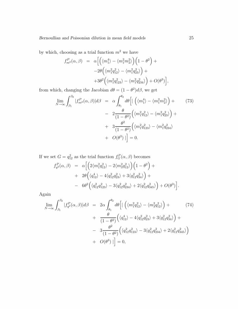
Bernoullian and Poissonian dilution in mean field models 25
by which, choosing as a trial function m2 we have
fPm2(α, β) = α
[(
〈m41〉 − 〈m2
1m22〉
)(
1 − θ2)
+
−2θ(
〈m21q
212〉 − 〈m2
1q223〉
)
+
+3θ2(
〈m21q
2123〉 − 〈m2
1q2234〉
)
+ O(θ3)]
,
from which, changing the Jacobian dθ = (1 − θ2)dβ, we get
limN→∞
∫ β2
β1
|fPm2(α, β)|dβ = α
∫ θ2
θ1
dθ[
|(
〈m41〉 − 〈m2
1m22〉
)
+ (73)
− 2θ
(1 − θ2)
(
〈m21q
212〉 − 〈m2
1q223〉
)
+
+ 3θ2
(1 − θ2)
(
〈m21q
2123〉 − 〈m2
1q2234〉
+ O(θ3) |]
= 0.
If we set G = q212 as the trial function fP
G (α, β) becomes
fPq2(α, β) = α
[(
2〈m21q
212〉 − 2〈m2
3q212〉
)(
1 − θ2)
+
+ 2θ(
〈q412〉 − 4〈q2
12q223〉 + 3〈q2
12q234〉
)
+
− 6θ2(
〈q212q
2123〉 − 3〈q2
12q2234〉 + 2〈q2
12q2345〉
)
+ O(θ3)]
.
Again
limN→∞
∫ β2
β1
|fPq2(α, β)|dβ = 2α
∫ θ2
θ1
dθ[
|(
〈m21q
212〉 − 〈m2
3q212〉
)
+ (74)
+θ
(1 − θ2)
(
〈q412〉 − 4〈q2
12q223〉 + 3〈q2
12q234〉
)
+
− 3θ2
(1 − θ2)
(
〈q212q
2123〉 − 3〈q2
12q2234〉 + 2〈q2
12q2345〉
)
+ O(θ3) |]
= 0,
26 Adriano Barra, Federico Camboni, Pierluigi Contucci
References
[1] E. Agliari, A. Barra, F. Camboni, Criticality in diluted ferromagnets, J.Stat. Mech. P1003 (2008).
[2] M. Aizenman, P. Contucci, On the stability of the quenched state in meanfield spin glass models, J. Stat. Phys. 92, 765-783 (1998).
[3] R. Albert, A. L. Barabasi Statistical mechanics of complex networks, Re-views of Modern Physics 74, 47-97 (2002).
[4] A. Barra, The mean field Ising model trhought interpolating techniques, J.Stat. Phys.145, 234-261, (2008).
[5] A. Barra Notes of ferromagnetic Pspin and REM, Math. Meth. Appl. Sci.,Wiley John and sons (2008)
[6] A. Barra, Irreducible free energy expansion and overlap locking in meanfield spin glasses, J. Stat. Phys. 123, 601-614 (2006).
[7] A. Barra, L. DeSanctis Stability properties and probability distribution ofmulti-overlaps in dilute spin glasses, Journal of Statistical Mechanics J.Stat. Mech. P08025 (2007).
[8] A. Barra, F. Guerra, About the ergodicity in Hopfield analogical neuralnetwork, J. Math. Phys. Special Issue ”Statistical Mechanics on RandomGraphs”, (2008).
[9] A. Barra, F. Guerra, Order parameters and their locking in analogical neu-ral networks, Dedicated Volume, Collana d’Ateneo, University of Salerno(2008).
[10] A. Barrat, M. Weight, On the properties of small world network models,Eur. Phys. Journ. B 13-3 (2000).
[11] A. Bianchi, P. Contucci, A. Knauf, Stochastically Stable Quenched Mea-sures, Journal of Statistical Physics, 117, 831-844, (2004).

Bernoullian and Poissonian dilution in mean field models 27
[12] M. Buchanan, Nexus: Small Worlds and the Groundbreaking Theory ofNetworks. Norton, W. W. Company, Inc. (2003).
[13] F. Chung, L. Lu, Complex Graphs and Networks, Americ. Math. Soc.Publ. (2006).
[14] P. Contucci, C. Giardina, The Ghirlanda-Guerra identities, J. Stat. Phys.,126, N. 4/5, 917-931, (2007).
[15] P. Contucci, C. Giardina, I. Nishimori, Spin Glass Identities and theNishimori Line, to appear in ”Progress in Probability”, (2008).
[16] P. Contucci, J. Lebowitz, Correlation Inequalities for Spin Glasses, An-nales Henri Poincare, 8, 1461-1467, (2007).
[17] P. Contucci, M. Degli Esposti, C. Giardina, S. Graffi, ThermodynamicalLimit for Correlated Gaussian Random Energy Models, Commun. in Math.Phys. 236, 55-63, (2003).
[18] R.S. Ellis, Large deviations and statistical mechanics, Springer, New York(1985).
[19] S. Ghirlanda, F. Guerra, General properties of overlap distributions indisordered spin systems. Towards Parisi ultrametricity, J. Phys. A, 31,9149-9155, (1998).
[20] F. Guerra, About the overlap distribution in mean field spin glass models,Int. Jou. Mod. Phys. B 10, 1675-1684, (1996).
[21] F. Guerra, L. De Sanctis, Mean field dilute ferromagnet I. High tempera-ture and zero temperature behavior, J. Stat. Phys. 129, 231, (2008).
[22] F. Guerra, F. L. Toninelli, The Thermodynamic Limit in Mean Field SpinGlass Models, Comm. Math. Phys. 230, 71-79, (2002).
[23] F. Guerra, F. L. Toninelli, The high temperature region of the Viana-Braydiluted spin glass model, J. Stat. Phys. 115, (2004).
[24] M.Mezard, G.Parisi, R. Zecchina, Analytic and Algorithmic Solution ofRandom Satisfiability Problems, Science 297, 812 (2002).

28 Adriano Barra, Federico Camboni, Pierluigi Contucci
[25] R. Monasson, S.Kirkpatrick, B.Selman, L.Troyansky, R. Zecchina, De-termining computational complexity from characteristic phase transitions,Nature 400, 133 (1999).
[26] M. Newman, D. Watts, A.-L. Barabasi The Structure and Dynamics ofNetworks, Princeton University Press, (2006).
[27] T. Nikoletoupolous, A.C.C. Coolen, I. Perez Castillo, N.S.Skantos, J.P.L.Hatchett, B. Wemmenthove, Replicated transfer matrix analysis of Isingspin models on small world lattices, J. Phys. A, 6455-6475 (2004).
[28] L. Pastur, M. Shcherbina, The absence of self-averaging of the order pa-rameter in the Sherrington-Kirkpatrick model, J. Stat. Phys. 62, 1-19,(1991).
[29] D.J. Watts, S.H. Strogatz, Collective dynamics of small world networks,Nature 393, 6684 (1998)