Robustness as a non-localizable relational phenomenon

Jose A. Fernandez-Leon*,†

Centre for Computational Neuroscience and Robotics, University of Sussex, Brighton BN1 9QG, UK

*E-mail: jafphd@gmail.com; jf76@sussex.ac.uk; Tel.: +44 (0)1273 872948; Fax: +44 (0)1273 678535.

†Present address: Department of Neurobiology and Anatomy, University of Texas–Houston Medical School, Houston, TX 77030, USA.

ABSTRACT

A current challenge in neuroscience, systems and theoretical biology is to understand

what properties allow organisms to exhibit and sustain behaviours despite perturbations

(behavioural robustness). Indeed, there are still significant theoretical difficulties in this

endeavour due to the context-dependent nature of the problem. Contrary to the common

view of biological robustness as a phenomenon that emerges internally, this article

discusses the hypothesis that behavioural robustness is rooted in dynamical processes that

distribute between internal controls, the organism body and the environment. This review

highlights the varied perspectives and how they have led to the current focus on

robustness as a relational phenomenon. A new perspective is proposed in which

robustness is better understood in the context of agent-environment dynamical couplings,

in which such couplings are not always the full determinants of robustness. The

challenges and limitations of the proposed approach are identified.

Key words: biological robustness, adaptive behaviour, minimal cognition, theoretical

biology, dynamical systems, bioinspiration.

CONTENTS

I.  INTRODUCTION ................................................................................................................................... 2 

II.  A HISTORICAL CONTEXT FOR SYSTEMIC ROBUSTNESS ...................................................... 3 

III.  ROBUSTNESS THROUGH DYNAMICALLY DISTRIBUTED MECHANISMS ...................... 16 

IV.  LIFETIME ROBUSTNESS, YET EVOLUTIONARILY CONSTRAINED ................................... 21 

V.  DISCUSSION: ROBUSTNESS AS A RELATIONAL PHENOMENON ...................................... 24 

VI.  CONCLUSIONS ................................................................................................................................... 30 

VIII. REFERENCES ........................................................................................................................................ 32 

IX. APPENDIX: BASIC CONCEPTS FROM NON-LINEAR DYNAMICAL SYSTEMS THEORY .. 36 

I. INTRODUCTION

Organisms’ surroundings play an important role in shaping their actions; behaviour is by

no means solely defined internally. The responses to particular situations in the

environment such as the presence of poisoned food where an organism cannot sense the

risk involved in eating it cannot be explained only in terms of the stimuli involved or

based on the organism’s internal structure. Furthermore, the same living being may

behave in completely different ways when presented with seemingly identical stimuli at

two different moments or places (Beer, 2004). In one case, the food may be consumed,

while in a different moment the organism may avoid the food because it has learnt the risk

involved (Beer & Chiel, 1990).

To account for these differences behavioural scientists usually assert that internal states

drive the changes in the organism’s response to its environment. Therefore, the

environment value is dependent on and regulated by the internal state of an organism

(further explained in Section II). However, this understanding of internal regulation

presents challenges on how to understand adaptive and persistent behaviours during an

organism’s lifetime. In this respect, when combined with environmental dynamics,

Maturana & Varela (Maturana & Varela, 1987) point out in that the ability of an organism

to draw these distinctions through its selective response to stimuli is a hallmark of

cognitive behaviour.

This review discusses the emergence of adaptive behaviours that outlast any initiating

stimulus arising from agent-environment interactions, and addresses current discussions

on behavioural robustness. The argument here is unique from other contributions in

theoretical biology and cognitive science in that it highlights a change in perspective on

robustness from being solely internally generated towards a relational phenomenon

involving agent–internal control, the body and the environment. Many of the pioneering

works in cybernetics suggest precisely this approach in a rich variety of ways, providing

a historical context for behavioural robustness research. The following discussions

outline how these studies have led to the current state-of-play in theoretical biology, and

draw conclusions on the relational domain of robustness.

II. A HISTORICAL CONTEXT FOR SYSTEMIC ROBUSTNESS

In 1932, while working at Bell Telephone Laboratories, Harry Nyquist provided the first

two measures of stability: gain and phase margins. In closed-loop control systems, phase

margin indicates relative stability − the tendency of a variable to oscillate during a

damped response to an input change (Healey, 1975). Damping is an effect that reduces the

amplitude of oscillations in an oscillatory system. Gain margin refers to absolute stability

and represents the degree to which a system will oscillate without limit given any

disturbance (Horowitz & Hill, 1989). Since that time, research on systemic resilience as

the ability to recover from or adjust to disturbances has been a topic of increasing interest

(Cogan, 2006).

Different, but connected, definitions of systems have appeared since that time in fields

like general systems theory (von Bertalanffy, 1968) and cybernetics (Ashby, 1956). For

example, von Bertalanffy (1968) proposed that a system is a set of interacting or

interdependent parts forming an integrated whole. Another definition (Ashby, 1960, p.16)

indicates that a system can be seen as “[...] any set of variables that [the observer or

experimenter] selects from those available on the real machine”. The latter description

identifies an important feature, emphasizing the role of the observer who selects the

variables, and whose intervention implies that any system is a mere abstraction.

Importantly, note that despite conceptual differences, systems in general share some

common characteristics: they have structure, that is, systems are defined by their

composition; they exhibit behaviour, which involves inputs, processing and outputs of

information; and systems have interconnectivity, where the various parts have

functional as well as structural relationships between each other (von Bertalanffy, 1968).

Here functional means systems (e.g. organisms, artificial agents, or robots) that are

capable of fulfilling a particular behaviour. ‘Structure’ refers to the components and

relations that constitute a particular unity and that makes its organization real (Maturana

& Varela, 1987).

These systemic characteristics also apply to living organisms. For example, von Uexküll

(1957) explained purposeful animal behaviour by joining an organism’s phenomenal

world (the interconnected information, and the world as perceived) and its effector world

[behaviour, and the world as enacted (De Jaegher & Di Paolo, 2013; Stewart, Gapenne &

Di Paolo, 2013)] into a single closed whole, the ‘Umwelt’ (Macinnes & Di Paolo, 2006).

Using his notion of Umwelt (or ‘self-centered world’ (Kull, 2010) , von Uexküll theorized

that organisms can have different internal environments or internal states, even though

they share the same environment. In his holistic view, von Uexküll (1957) proposed

multidisciplinary discussions in fields like muscular physiology, animal behaviour

studies, and the cybernetics of life. In his terms, the selection of sensory stimuli can be

seen as a process that can bring forth organisms’ own relevance in the surrounding world.

Importantly, this idea suggests that behavioural mechanisms can be thought as cognitively

distributed between internal control, body, and environment.

von Uexküll’s (von Uexküll, 1926; von Uexküll, 1957) description of functional circles

between the organism and the environment suggests that a ‘cue’ (or functional trigger) is

distributed along the functional circle of which the organism is a part (Fig. 1). In this

context, functional circles are abstract structures that tie together a subjective experience

or perception (termed a perceptual cue) and the effect that the perceptual cue has on the

behaviour of the organism (called an effector cue) (Macinnes & Di Paolo, 2006; von

Uexküll, 1926; von Uexküll, 1957). It is meaningless, therefore, to claim that a perceptual

cue resides in a particular location in the organism’s internal milieu. For example, the

ability to walk and the feedback that the nervous system receives during walking is not

localized at the neural level but is fully distributed throughout the organism and its

dynamics, where part of the control task is ‘outsourced’ to the physical dynamics of the

body (Pfeifer & Scheier, 2001).

This dominating motif in biological thinking was introduced earlier by the physiologist

Claude Bernard (Gross, 1998). He was the first to define the term ‘milieu intérieur’,

currently known as homeostasis. He summarized his idea as follows: “The fixity of the

milieu supposes a perfection of the organism such that the external variations are at each

instant compensated for and equilibrated [...] All of the vital mechanisms, however varied

they may be, have always one goal, to maintain the uniformity of the conditions of life in

the internal environment [...] The stability of the internal environment is the condition for

the free and independent life.” (Gross, 2009), p. 193)(Bernard, 1974). This understanding

implies that stability is a major organizing physiological principle in which the constancy

of the ‘internal environment’ must be maintained in the face of regulating this

environment in terms of temperature, acidity, ionic composition and so forth, in

multicellular organisms.

The concept of homeostasis, however, constrains our view of living systems in that the set

points are not themselves constant during homeostatic regulation, but change over time as

an open system (von Bertalanffy, 1968). In fact, the concept of homeostasis has recently

shifted to a richer concept, that of ‘homeodynamics’. This new concept sees dynamic

organization under homeostatic conditions that make possible the organized complexity

of life (Ikegami & Suzuki, 2008; Lloyd, Aon & Cortassa, 2001). Homeodynamics

conceptualizes the ability dynamically to self-organize behaviour where there is a loss of

stability. More specifically, homeodynamics as a concept emphasizes the stability of the

internal milieu towards perturbation. Since the second half of the 20th century, theories on

self-organization (Ashby, 1947; Ashby, 1962; Glansdorff & Prigogine, 1971) and

dynamic systems (Strogatz, 1994) have allowed us to approach the quantitative and

qualitative analysis of the organized complexity that characterizes homeodynamics

(Lloyd et al., 2001). For example, focusing on homeostatic regulation of sensorimotor

coupling in artificial life (AL) and complex systems, Ikegami & Suzuki (2008) reported a

mechanism that drives a homeostatic state to an autonomous self-moving state in

computational cell models. The mechanism is similar to with Ashby’s (1960)

ultrastability concept, where random parameter searching is activated when a system

breaks a viability constraint on a modelled internal variable in cellular organisms. This

random search changes the interconnectivity of the system (i.e. of the cellular organisms).

Further evidence that both self-organization and a rich complex initial state are required

for biological robustness is reported in (Hanczyc & Ikegami, 2009). The balancing act

between these two factors (self-organization and a rich complex initial state) is the

‘Maximalism Design Principle’ for biological robustness (Silverman & Ikegami, 2010).

This principle proposes that a biologically plausible minimal cell cannot be found using

traditional laboratory approaches and protocols and challenges today’s experimentalists to

design more complex initial states (Hanczyc & Ikegami, 2009).

The above examples of novel studies provide some insights into factors that contribute to

homodynamic regulation. While these examples illuminate some possibilities for

developing studies on homeodynamics, among other themes, how might such a

comprehensive approach assist our effort to study a common mechanism for adaptive

regulation? Ashby (1960) argued that all adaptive organisms have regulatory

mechanisms. He proposed a universal mechanism with an output to the environment and

at least two feedback loops (Fig. 2). A primary loop enables the organism to interact with

the environment via sensorimotor feedback, and a second loop that connects the

environment to the essential variables. These essential variables can consecutively affect

the organism’s sub-systems causing a change at the organism level. Fig. 2 shows the

sensorimotor loop represented by arrows to and from the sub-system R. Those parameters

(S) that affect R have an immediate effect on the subsystem’s behaviour, but not on the

environment. E represents the essential variables having an effect on S. Homeostatic

regulation is represented as a dial with limit marks representing their boundaries. When

the essential variables exceed the limits, they cause S to change in value by means of this

step mechanism. In this way, the system can maintain a particular steady state or reach a

new one in state space (see Appendix). Thus, an idealized, simple mechanism is sufficient

to drive adaptive changes towards stable states in living organisms. Furthermore,

according to Ashby’s Law of Requisite Variety, different types of perturbations often

require different counter responses (including regulatory ones) which can be understood

as a system reaching one of several steady states (see Appendix). More importantly, his

law indicates that the larger is the variety of actions available to a control system, the

larger the variety of perturbations it is able to compensate (Ashby, 1958; Ashby, 1960).

Adaptation in Ashby’s conceptual framework enabled discussions on ultrastability that

can be understood as multistability (see Appendix). Ultrastability can be defined as the

ability of a system to modify internal relationships and/or to influence environmental

conditions to maintain stability (Ashby, 1960). This stability can be affected by small or

larger perturbations to essential variables. Small perturbations can be caused by the

organism–environment coupling via the sensorimotor loop (Fig. 2) or when the essential

variables approach or exceed their bounds. Usually, larger perturbations will induce a

change in the subsystem S that will force the organism to find a new equilibrium by

changes in its behaviour. In this way, Ashby (1960) demonstrated how adaptive systems

lead to a variety of different behaviours, and showed the effectiveness of a multistable

system in searching for stable equilibriums when perturbed. For example, in one of the

few applications of Ashby’s ultrastability, Di Paolo (Di Paolo, 2000) applied homeostatic

regulation of synaptic activity to the evolution of organisms. His experiments were on

adaptation to left/right visual inversion (Held, 1965; Kohler, 1962) using a goal-

approaching robot controlled by the individual activity of artificial neurons as essential

variables. When sensors were inverted, the robot became unstable and started to change in

terms of its internal states. Eventually, the goal-approaching behaviour was regained (Di

Paolo, 2000). Even though the organisms were not designed specifically for this task, Di

Paolo (2000) showed that they could adapt to sensory inversion. Adaptation in Di Paolo’s

(2000) experiments emphasized the stability of the internal milieu towards perturbation,

but left open discussions on the mechanism that drives adaptation in more complex

models. Di Paolo (2000) further discussed how ultrastability leads to adaptation and its

link to behaviour.

von Neumann (von Neumann, 1956; von Neumann, 1966; von Neumann, 1987) earlier

noted the complexity of understanding how a system can resist changes to its initial

configuration by opening debates on the synthesis of reliable organisms from unreliable

components. Reliability here indicates the ability of artificial or biological organisms to

maintain their functionalities in normal (unperturbed) situations (e.g. walking behaviour

in non-uniform slope terrains) (Ashby, 1960; Stebbing, 2009). von Neumann’s notion of

one robot building another robot is known as the von Neumann’s kinematic model of

self-reproduction (von Neumann, 1966). His idea of a universal constructor, however, has

never been subject to physical implementation, because the fragility of the modelled

machines against unavoidable perturbations was drastic compared to more natural

kinematic settings (Friedman, 1996; Sayama, 1996)). These early ideas opened debates on

whether cybernetics can copy mechanisms observed in the biological realm to implement

them in artificial or robotic systems (Ashby, 1956; Ashby, 1960; Ashby, 1981).

The main difference between these types of systems is that in robots, designers impose

internal and external requirements that must be obeyed [e.g. the generation of moving-

home actions when the robots’ batteries are low (Nolfi & Floreano, 2000)]. Conversely,

biological organisms are guided mostly by what their metabolism dictates (Boden, 1999).

For instance, Cannon (Cannon, 1939) discussed his understanding of homeostasis by

using experiments from cybernetics describing self-regulating mechanisms that preserve

essential physiological variables (e.g. body temperature) in a state of dynamic balance.

More specifically, Cannon (1939) generalized Bernard’s concept introducing the term

homeostasis as the tendency of a self-regulated system to maintain its essential variables

close to some fixed point, like the temperature of a room controlled by a central heating

system and a thermostat. Note, however, that homeostasis only maintains a physiological

state and not necessarily full systemic functions (Kitano, 2004). Kitano’s perspective

suggests that the continuation of organism’s functions usually (but not exclusively)

implies an active and flexible internal control (see also (Ikegami & Suzuki, 2008;

Silverman & Ikegami, 2010).

The above examples indicate that usually the system under study is the organism, rather

than the interactions between internal control and environmental dynamics. Alternatively,

Beer (1997) proposes that focusing on the organism’s internal structure as a system does

not necessarily exclude the outside environment (Fig. 3). In fact, the internal structure of

an organism, its body and its environment can be a rich, complicated, highly structured,

coupled dynamical system, and behaviour can emerge from the adaptive interactions of

all three components as a system (Fig. 4) (Beer, 1997). However, such complexity implies

that the understanding of some phenomena such as behavioural robustness and

adaptability is a delicate task. For instance, it is relatively easy to produce artificial

organisms exhibiting particular behaviours, but identifying the associated processes in

living organisms is generally not trivial (Beer, 2000; Nolfi & Floreano, 2000; Silverman

& Ikegami, 2010). One difficulty arises in that the number of concurrent behavioural

processes in most biological organisms is higher than those in artificial systems.

The following discussions employ the definition of a system as an agent (organism or

robot) and its environment (agent–environment system) (Fig. 4C), using the term inner

system when necessary to refer to the agent’s internal features (Fig. 4A). In Fig. 4

different dynamical loops (grey circles) contribute to sustain behaviours despite internal

malfunctions and external perturbations. Fig. 4B represents the adaptive behaviour

approach which proposes that the nervous system (NS) is embedded within a body, which

in turn is embedded within the environment. Fig. 4C illustrates the case in which the

internal activity of an agent is dependent on and continuously perturbed by dynamical

cycles between internal control, body and environment, with no necessarily separable

inner mechanisms producing robustness (see also (von Bertalanffy, 1968), p. 106). In this

case adaptive behaviour emerges from the interactions of all three sub-parts (nervous

system, body, and environment), where the highly recursive and integrated activities of

these parts are in constant flux and open to body and environment dynamics (dashed lines

in Fig. 4C).

To understand better the complexity of the agent–environment problem, consider the case

of adaptability and structural stability. Adaptability here refers to the capacity of an

organism to regulate itself within the boundaries of its own internally defined properties

(Di Paolo, 2005), p. 429). In brief, the established theory of adaptive systems tells us that

biological organisms typically (but not exclusively) reorganize their components and in

doing so they remain functional and stable after perturbations (Ashby, 1940; Ashby,

1960). Adaptive capacity is commonly discussed in the context of the nervous system

co-developing with the body and the dynamics of the environment (Chiel & Beer, 1997;

Gallagher, 2005). Ashby (1960, p.58) gives a behavioural interpretation of this concept:

“behaviour is adaptive if it maintains the essential variables within physiological limits”

(see also (Umpleby, 2009). Note that adaptive capacity, however, does not always

produce better outcomes because it can lead to the exhaustion of adaptive resources,

malfunction of regulation, and loss of adaptive buffering provoking the activation of

extreme regulation (Di Paolo, 2005).

The concept of systemic stability has produced increasing interest in understanding how

biological systems remain functional to certain perturbations. According to (Jen, 2003), p.

2), “[a] dynamical system is said to be structurally stable if small perturbations to the

system result in a new dynamical system with qualitatively the same dynamics”. In

(Strogatz, 1994), this concept is argued mathematically as the stability of the flow in a

phase space (see Appendix). Briefly speaking, if a perturbation does not change the

topological relationship of the flow, we say it is structurally stable. For example, assume

that the flow of water in a river only depends on wind speed, the flow is structurally stable

to wind speed variations if small changes in wind speed do not qualitatively modify the

dynamics of the flow by producing a new structure, such as an eddy (Diacu & Holmes,

1996; Jen, 2003). In non-biological systems, like a river, this observation shows the

existence of different responses that depend on the magnitude of external changes.

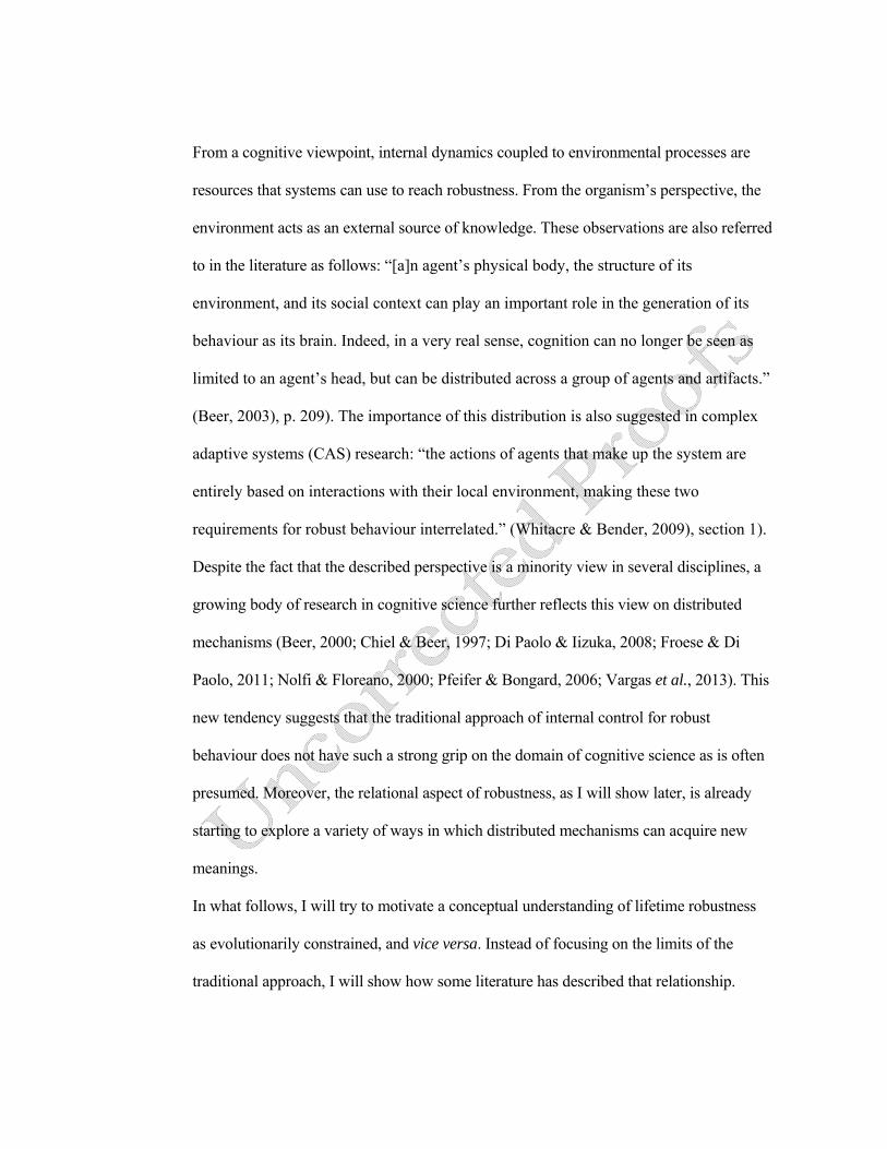
Fig. 5 shows schematics of environmental influences and the effect of perturbations on

inner dynamics. In Fig. 5A, two environments are shown (rich and minimal media). The

agent–internal system selects cues available in the environment (via the body sensing) and

responds with actions in the environment. Cues are information inputs to inner control

and are deemed essential to accomplish actions. Fig. 5B demonstrates the situation in

which a current state of an internal control can be modified by small or large perturbations

pushing the agent–internal dynamics within the current boundary of attraction or far from

it (see Appendix). Perturbations may produce a dynamical return to the pre-perturbation

state, dynamical changes toward different steady states, or push current dynamics toward

an unstable region (from which the dynamics will eventually return if possible). In this

way, when an organism with such dynamics remains functional despite perturbations, the

changes of regions can be part of the robust response needed to reach stability.

Both concepts, adaptability and structural stability, intuitively indicate that three common

outcomes can arise from perturbations (Kitano, 2007), p. 137) (see also Appendix): (a)

the system cannot tolerate perturbations and it is no longer functional – it is not able to

sustain the original functionality; (b) the system compensates for effects of perturbations

and maintains a steady state – the system will continue in its current state; (c) the system

changes to another stable, functional configuration (Fig. 5B). An example of this is the

amoebic cyst process that is activated when the environment is potentially lethal. During

this process, an amoeba may pass from being mobile (b) to another state (c) where it

becomes dormant by forming a microbial cyst. The cell remains in this state until it

encounters more favourable environmental conditions (c) or eventually dies (a) (Leidy,

1878). The last outcome (c) commonly implies multi-stability at the systemic level to

radical changes in the face of perturbations (Ashby, 1960), p. 209; (Anderson, 2002). In

this context, once again, multi-stability refers to a systemic property that enables a system

to maintain its functions despite perturbation by reaching one of several (equally

functional) steady states.

These three outcomes suggest that robustness as a property of biological organisms does

not exclusively convey stability but also can entail adaptive controls. For instance,

imagine two organisms moving from A to B, two distant points in physical space, while a

predator is trying to catch them. The first organism, which relies extensively on internal

state variables will typically move in a predictable path and thus be caught and killed.

This behaviour can be guided by strategies and modulation of risk attitudes in the

organism’s response. More specifically, this organism’s decision could depend on state

variables associated with the animal’s risk attitudes towards behaving differently when

detecting a predator guided by its belief on how to behave (further explained below). A

second organism dodges left and right in response to incoming signals based on the

movements of the predator. This might make the second organism more likely to survive.

Note also that during interaction with its near environment, not only can an organism rely

on internal control for robust, yet adaptive behaviour, but also on body features. For

example, insects such as moths and butterflies can fly pseudo-randomly due to wing

design and wing movements and thus hinder predation. Both examples suggest that

organisms can remain functional by producing changes at the internal (e.g. based on

flexible sensorimotor control) and environmental level (e.g. behavioural escape

movements). Furthermore, whereas an organism’s internal control may be the prime

mechanism for handling certain types of perturbations, biological organisms can also use

body–environment dynamics to mitigate the effect of perturbations (Fig. 4C). For

example, most desert animals avoid the sun during the hottest part of the day by looking

for refuges, and desert mammals, reptiles and amphibians live in burrows to escape the

intense desert heat. Behavioural actions like these may be required to sustain essential

physiological functions, but they are not solely ensured by internal controls (cf. (Kitano,

2004; Kitano, 2007; Krakauer, 2005). We can ask consequently whether it is reasonable

to assume that the environment is part of the system under study, or if it represents

another part that only perturbs the organism’s decisions as a system (Fig. 5A).

The above examples serve to illustrate the importance of complex interactions with the

environment, which can lead to the later development of robust and adaptive behaviours.

However, an organism avoiding its predator, or any risky situation, may be seen as an act

of robustness. This interpretation could create the illusion of pushing the robustness term

too far, to the point that it becomes useless. However, from a phenomenological

standpoint, biological systems from unicellular to whole organisms are robust if they

continue to function, survive or reproduce when faced with mutations, environmental

change and internal noise (Wagner, 2007). In particular, survival as the struggle to remain

living refers to the ability to perform a variety of behaviours aimed at survival: motility,

avoiding predators, and eating, among others. (Whitacre, 2012) notes that environmental

tracking by means of movements within the environment [e.g. chemotaxis (Alon et al.,

1999) and predator avoidance (Kondoh, 2007)] can alter the perturbations a system is

exposed to. Those alterations can improve the robustness of an organism and

alternatively, organisms and biological subsystems can offset the negative influence of

their surroundings. One example of this is the amoeba cyst process (Leidy, 1878)

discussed above. Other examples of behaviour supporting robustness can be found

throughout biology (Edelman, 1987). However, few studies discuss those strategies for

achieving behavioural robustness as a relational phenomenon between internal control

(e.g. homeostatic regulations) and behaviour (e.g. environmental tracking).

The next challenge is to scale up this discussion from internal control mechanisms to

distributed control. As I will now show, many published papers in theoretical systems

biology and cognitive sciences do support this in a rich variety of ways.

III. ROBUSTNESS THROUGH DYNAMICALLY DISTRIBUTED

MECHANISMS

In a series of recent papers, Kitano argued that the cooperative work of systemic

components, like nerves in the brain, is what enables the functional maintenance of a

system (Kitano, 2007), p. 1). More specifically, he says that: “the coordinated

physiological processes which maintain most of the steady states in the organism […]

involving, as they may, the brain and nerves, […], all [work] cooperatively […].” This

claim, while interesting, still views robustness as an internal property within the organism

in the form of network organization. In fact, the word ‘distributed’ in neuroscience and

artificial intelligence, among other fields, still means ‘distributed within the brain’ (i.e.

like distributed parallel computation in neural networks; (Arbib, 1995).

A theoretical holistic approach in these fields usually implies that organisms obtain

information from the environment (including the body) in a way no dedicated internal

control system could possibly emulate (Espenschied et al., 1996; Pfeifer & Bongard,

2006; Pfeifer & Scheier, 2001; Scheier, Pfeifer & Kunyioshi, 1998). Krakauer (2005,

section 3.6.) describes such a distribution as follows: “distributed processing, or

connectionism, might be assumed to be a combination of modularity and spatial

compartmentalization, but differs in that a single function is emergent from the collective

activities of units, and correlated activity is thereby a desired outcome.” His observation

suggests that distributed processes are beneficial for robustness in connectionist models

due to graceful degrading upon removal of individual nodes. This idea is usually

associated with structural and organizational properties of the nervous system like

modularity and redundancy (Csete & Doyle, 2002; Csete & Doyle, 2004; Godzik,

Schoenauer & Sebag, 2004; Kitano, 2004; Kitano, 2007; Krakauer, 2005; Lesne, 2008).

In biology, modularity refers to components (or metabolic pathways) each with specific

functions. Redundancy implies similar functionality across those components or pathways

(Fig. 6A). Félix & Wagner (2008) reported that redundancy is one way of favouring the

robustness of the system, but the presence of excessive redundancy may increase the

effort required to sustain information (Fernandez & Solé, 2004; von Neumann, 1966;

Wagner, 2005). Fig. 6B shows the relation between processes that are seen as distributed

robustness. These processes are robust because the flow of information is distributed

among several alternative components and flow paths, with no two parts performing the

same function. By contrast, if robustness is achieved through redundancy (Fig. 6A),

several components perform the same function.

Even at the level of internal physiology, it is important not to misunderstand the notion of

internal control as merely a kind of physical structure. Rather than being a response to

internal and external perturbations, which is how robust control was typically defined in

cybernetics, robustness in systems biology is now conceived as distributed. In this respect,

Macía & Solé (2008, section 5) state that “[…] as found in biological systems, we can

see that the origins of robustness against the failure of a given element are largely

associated with a distributed mechanism of network organization.” This perspective on

distributed mechanisms suggests that, for example, the nervous system can be seen as the

sole generator of internal activity relevant to behaviour (Farah, 1994; Kien & Altman,

1995); however, sometimes the rest of the body may also be relevant (Clark & Chalmers,

1998; Gallagher, 2005).

The concept of distributed robustness is gaining awareness in systems biology and other

fields (Calcott, 2010; Wimsatt, 2007) in that interactions of multiple parts each with a

different role can compensate for the effects of perturbations by means of ‘degeneracy’

(Félix & Wagner, 2008; Wagner, 2005). This concept refers to the ability of elements that

are structurally different to perform the same function (Fig. 6B) (Edelman & Gally, 2001;

Tononi, Sporns & Edelman, 1999). Despite the importance of degeneracy in explaining

distributed robustness (Wagner, 2005), this concept still deserves further investigation

mainly because it conveys intrinsic complexity of information flow. For example,

biological neural networks working as control systems are highly robust to removal of

synapses or neurons regardless of populations of neurons having different roles (Amit,

1989; Beer, 1995; Clark & Chalmers, 1998; Gallagher, 2005). The distributed processing

is consequently an integrated set of functionalities that are commonly performed by

multiple, semiautonomous units or groups of them (McClelland, 1989). More

importantly, the relationship between the distributed flow of information and the effect of

perturbation on such flow is still not easy to comprehend or replicate.

Behavioural mechanisms that distribute across the brain–body–environment might be

thought of as an additional protection against changes that threaten crucial biological

functions (cf. (Hunter, 2009; Macía & Solé, 2008; Wagner, 2005). In the context of

adaptive behaviour, Chiel & Beer (1997) and Chiel et al. (2009) stated that the nervous

system cannot process information not transduced by the body. The converse idea

suggests that properties of the body may simplify complex neural processing by using

different body dynamics and sensorimotor information. For example, to keep our torso

stable and conserve energy, we swing our arms backwards and forwards and engage in a

swing/stance cycle of our legs while walking based on foot and equilibrium feedbacks.

Some studies in cognitive science (Beer, 1995) have discussed the dynamical role of

brain, body and environment in behaviour (Fig. 4B), rather than concentrating on the

nervous system (as a control system), or its parts, as the sole behaviour producer (Fig.

4A). Here we have the beginnings of the idea that distributed mechanisms go beyond

structural functionalism. Nevertheless, there are many definitions of mechanisms in the

philosophy of science and biology. These definitions also highlight the idea of

distributed dynamics, rather than focusing on the structural properties of systems. One

influential characterization of neurobiological mechanisms is: “mechanisms are entities

and activities organized such that they are productive of regular changes from start to

termination conditions” (Machamer, Darden & Craver, 2000), section 2). From an

epistemic standpoint, the orthodox view of mechanisms as internally placed implies that

mechanisms are dynamic producers of a certain phenomenon of interest (Ashby, 1940;

Nolfi & Floreano, 2000). Kitano (2002, p. 1662) suggests that this traditional

perspective hinders understanding of the mechanistic, system-wide basis of robustness

arguing that “[t]o understand biology at the system level, we must examine the structure

and dynamics of cellular and organismal function, rather than the characteristics of

isolated parts of a cell or organism.”

Recent work in theoretical neuroscience argues that the division between behavioural

mechanisms and mechanisms generating robust traits is not straightforward. New

evidence that “the body shapes the way we think” (Pfeifer & Bongard, 2006), indicates

that the full experience of body–environment coupled dynamics continuously shapes

cognitive and behavioural abilities as well as their respective mechanisms (Fig. 4C). In

this respect, (Di Paolo, 2009) implies that cognition is a relational phenomenon of brain,

body, and environment, and thereby is not localizable (see (Ashby, 1960), p. 70).

Likewise, neuroscience and cognitive science are beginning to show how behaviour and

cognition arise as a relational phenomenon, which has an impact on behavioural

robustness research.

From a cognitive viewpoint, internal dynamics coupled to environmental processes are

resources that systems can use to reach robustness. From the organism’s perspective, the

environment acts as an external source of knowledge. These observations are also referred

to in the literature as follows: “[a]n agent’s physical body, the structure of its

environment, and its social context can play an important role in the generation of its

behaviour as its brain. Indeed, in a very real sense, cognition can no longer be seen as

limited to an agent’s head, but can be distributed across a group of agents and artifacts.”

(Beer, 2003), p. 209). The importance of this distribution is also suggested in complex

adaptive systems (CAS) research: “the actions of agents that make up the system are

entirely based on interactions with their local environment, making these two

requirements for robust behaviour interrelated.” (Whitacre & Bender, 2009), section 1).

Despite the fact that the described perspective is a minority view in several disciplines, a

growing body of research in cognitive science further reflects this view on distributed

mechanisms (Beer, 2000; Chiel & Beer, 1997; Di Paolo & Iizuka, 2008; Froese & Di

Paolo, 2011; Nolfi & Floreano, 2000; Pfeifer & Bongard, 2006; Vargas et al., 2013). This

new tendency suggests that the traditional approach of internal control for robust

behaviour does not have such a strong grip on the domain of cognitive science as is often

presumed. Moreover, the relational aspect of robustness, as I will show later, is already

starting to explore a variety of ways in which distributed mechanisms can acquire new

meanings.

In what follows, I will try to motivate a conceptual understanding of lifetime robustness

as evolutionarily constrained, and vice versa. Instead of focusing on the limits of the

traditional approach, I will show how some literature has described that relationship.

IV. LIFETIME ROBUSTNESS, YET EVOLUTIONARILY CONSTRAINED

Before proposing a definition of robustness that conveys meaning for the ‘distributed

mechanism hypothesis’, we must develop conceptually a firmer relationship between two

senses of robustness: robustness at the evolutionary and lifetime level.

Discussions herein focus on lifetime robustness concentrating on whole-organism–

environment dynamics. This decision avoids the drawbacks of studying robustness at the

evolutionary level (Wagner, 2007), since during evolution the coupled interactions of

agents with their environments are difficult to explore. Nevertheless, the relationship

between evolutionary robustness and robustness during an organism’s lifetime exists. For

instance, (Cogan, 2006), p. 20) suggests that “[r]obustness is the fundamental organising

principle of evolving dynamic systems such as biological systems. One could say that

robustness allows evolution to happen and that evolution favours robustness.”

The core of the paradigm of evolution influencing lifetime robustness, and vice versa,

mainly arises from the notion of phenotypic expression and fitness landscape. For

instance, suppose that we have found two different organisms (phenotypes) from the same

population. We can discover that both phenotypes show quantitatively similar behavioural

performance (fitness) under the same experimental conditions. After inducing mutational

changes in the organisms’ genes at the genotypic stage, we can measure a decrease in

fitness in one of the organisms at the phenotypic stage. This indicates less resilience to

certain perturbations during an organism’s lifetime. In other words, the negatively

affected phenotype suggests a decrease in fitness with respect to a certain amount of

mutation induced in the phenotype exhibiting no decay in fitness. Fitness is hard to define

strictly across organism–environment systems, but it refers to a relative quantitative

measure that helps to express the relationship between a certain perturbation on a control

variable and the resulting performance. A change in fitness can indicate less robustness

with respect to tasks that an organism should be able to accomplish (Nolfi & Floreano,

2000; Pfeifer & Bongard, 2006).

Following Burch & Chao’s (2000) arguments, we can see that such differentiation in

fitness is caused by mutations where the mutated phenotype is placed in the

multidimensional fitness landscape (i.e. a mathematical representation plotting change in

perturbed variables against level of fitness). Fig. 7 shows plots where the x and y axes

represent sequence space. The coloured dark grey surface is the fitness plane measured

during the phenotypic lifetime. Phenotypes showing decay in performance after mutation

induction are usually found in high fitness peaks before the perturbation (Fig. 7A). A

mutated phenotype showing no decay of fitness will be in a flatter region of the fitness

surface with relatively equal fitness compared to its non-mutated genotypic expression

(Fig. 7B). The resulting phenotype of the non-affected genotype therefore is more robust

with respect to induced mutations than another phenotype showing decay in fitness (see

(Elena & Sanjuán, 2003; Wilke & Adami, 2003; Wilke et al., 2001). However, as

Silverman & Ikegami (2010) discussed, some individuals of a population can display

robustness, but that does not indicate that the population as a whole is robust.

The notion of interrelating lifetime and evolutionary robustness, in combination with the

idea of robustness at the relational level, has had the effect of making some orthodox

definitions of robustness uncomfortable. In this respect, the definition of robustness can

be redefined considering several arguments reported herein. Typical definitions found in

the literature are also presented for contextual purposes.

Different meanings of robustness have been extensively reported in biology and

engineering (Calcott, 2010; Jen, 2003; Lesne, 2008). In a metabolic context, robustness

relates to limited phenotypic variation across large changes in kinetic parameters (Hurst &

Randerson, 2000; Westerhoff, Groen & Wanders, 1984). Another description from

systems biology is: “[robustness refers to] the ability to maintain performance in the face

of perturbations and uncertainty” (Stelling et al., 2004), p.675). Krakauer (2005, p.186)

also proposes that “robustness relates to two critical properties of complex biosystems:

the long-term limits to evolutionary change and the short-term persistence of system

function”. Conversely, he indicates that robustness mechanisms are one of the bridges

connecting the dynamics of ontogeny with those of phylogeny by limiting phenotypic

variation and providing the means to explore alternative genotypes without compromising

the phenotype. Despite the context dependence of his observation, Krakauer (2005)

suggests an important distinction between genotypic and environmental robustness. In the

former, perturbations (e.g. gene mutations) are inherited (de Visser et al., 2003), whereas

in the latter case they are not (Hagen & Hammerstein, 2005). These definitions, however,

hardly connect each other but the overall observation is that robustness is a phenomenon

that allows a system to maintain functionality against internal and external perturbations.

Because it is important to choose an appropriate description, I propose that: robustness is

the capacity that allows an agent (artificial or biological) to continue functioning via

tolerance or adaptation to internal and external perturbations, where this capacity is

partially determined by an agent–environment history of interactions. It is informative

then to define robustness as a property of an organism (or artificial agent) coupled to an

environment in the presence of perturbations (Fernandez-Leon, 2012). This definition

involves those situations in which an agent develops endurance to resisting perturbations,

and situations to which an agent has not developed tolerance (e.g. situations not present

during its evolution or during its lifetime history). Furthermore, this definition enables

sensible discussion of circumstances in which an agent is robust (e.g. specific

perturbations that were present during its development and evolution) and the

functionality that is maintained despite perturbations due to tolerance or changes in the

dynamics of the agent–body–environment. It also allows the possibility of perturbing the

inner organism (e.g. part of the nervous system), a trait (e.g. shape of the organism’s body

through mutilation), or a capability (e.g. sensory capacity). Furthermore, it is compatible

with a measurable notion of behavioural robustness, usually called fitness (Nolfi &

Floreano, 2000). Importantly, it is worth noting that robustness as defined herein does not

deny the relevance of internal mechanisms sustaining (instead of ensuring) a high degree

of robustness in cases of unforeseen environmental or internal changes. In fact, internal

control systems remain the most active element when understanding behaviours under

perturbations. This new definition, however, opposes the idea of an absolute role of

internal control for understanding robust capacities.

These reflections raise the question of how we can localize mechanisms in order to

account for the eventual emergence of robustness. In what follows, I will briefly consider

how to address this latter aspect.

V. DISCUSSION: ROBUSTNESS AS A RELATIONAL PHENOMENON

Previous sections presented new arguments that the maintenance of cognitive actions and

behaviours under perturbations depend deeply on the shape and structure of agent–

environment dynamics. Examples of this dependence were discussed above; see also

Ashby’s work on ultrastability (Ashby, 1960), and Di Paolo’s homeo-adaptation with the

inverse visual-sensors experiment (Di Paolo, 2000). This argument opposes the idea that

the maintenance of functionalities in behavioural systems is solely determined by the

agent’s internal structure. Unfortunately, this relationship between robustness and coupled

dynamics is rarely discussed in theoretical biology. There is plenty of work, however, on

what types of inner structures will tend to be robust as extensively presented herein (see

(Kitano, 2004; Krakauer, 2005; Wagner, 2007; Whitacre, 2012). Further, most of the

literature tends to show a one-sided view of the problem, focusing on the organism

dynamics and not on the dynamics of the coupling. If we are to take the study of lifetime

robustness seriously, we should carefully scrutinize the traditional notion that agent–

internal mechanisms ensure robustness.

A potential criticism of the approach presented herein is that behavioural robustness is

described based on a set of environmental changes (e.g., some living systems are robust to

working in the air or under water). Consequently, it might be thought that robustness

cannot be defined as a property of a system in interaction. However, this review claims

that robustness is a property of an agent in isolation (e.g. a robot is made of metal which is

robust to certain environmental conditions that do not affect metals). Robustness is also

inherently a property of the coupled agent–environment when some functionality is

maintained by the fully coupled system. This is explored below.

There are several possible claims for the distribution of mechanisms: (a) robustness

always depends on the agent–environment coupling; (b) robustness sometimes depends on

the agent–environment coupling; (c) robustness often depends on the agent–environment

coupling; (d) for certain kinds of systems, robustness strongly depends on the agent–

environment coupling; (e) robustness is understood better in the context of agent–

environment coupling. Claim (e) is slightly weaker than other claims because it does not

require that the agent–environment dynamics are the determinants of robustness in all

cases, although this also can be claimed for cases (b), (c), or (d). The dependence of

robustness to agent–environment coupling is the strongest option for claim (a), but I

believe that this claim is false. This article defends claim (e) but it also supports claim (b).

Claims (c) and (d) are more interesting: (c) because it proposes that one can expect in

general some tendency to observe agent–environment dynamics for robust behaviour, and

(d) because it prompts the question, which kind of system tends to rely more on agent–

environment dynamics? However, claims (c) and (d) are difficult to defend based on

discussions presented herein, because one needs to identify how often behavioural

robustness depends on agent–environment dynamical engagements or to classify types of

systems where robustness depends strongly on coupling.

Discussions in this paper highlight claim (b); robustness sometimes depends on the agent–

environment coupling. In other words, it is not generally appropriate to assume that the

ability to categorize, recognize, and exhibit behaviours in normal situations and under

perturbations is intrinsically a matter of agent–internal processes, and only extrinsically

related to bodily inputs and dynamics. These observations suggest that specific

environment-engaging loops and patterns of body dynamics make an essential difference

in how agents perceive the world and sustain robust behaviours. Thus, how can one

compare the distribution of a behavioural control system in relation to another system?

There are different ways to account for the distribution of a control system, which

depends on how it is hypothesized that processes split between the brain, body and

environment. For instance, the distribution criterion can be defined based on the role of

functional dependencies between an agent’s inner control system and outer environmental

dynamics (including the body). These dependencies can be rooted in coupled dynamics

that emerge from mechanisms that organisms develop for behavioural modulation (Chiel

& Beer, 1997). (Fernandez-Leon, 2012) proposed that such an identification of functional

dependencies could be based on perturbation analysis. For example, from a modelling

perspective of artificial systems, it is possible to study the effects of reducing incoming

signals (sensory feedback) in agents showing walking behaviour (Fernandez-Leon, 2011).

In this scenario, we can explore whether further dependence on sensory feedback from an

agent’s leg can be measured as decay in performance when perturbed. This is a useful

method to account for the distribution of cognitive and behavioural mechanisms in agents.

This method allows investigation into the specific ways in which the system-in-coupling

can be behaviourally robust.

Another possible alternative for practicing biologists is by studying causal contributions

using Granger Causality (G-causality) from the computational neuroscience field (Seth,

2005; Seth & Edelman, 2007). This type of analysis can be used to explain the joint

product of network structure and the dynamical processes operating on that structure,

which may be modulated by environment and context. Seth & Edelman (2007) show how

the same network structure can generate different causal networks depending on context.

G-causality has been applied to simulated neural systems to probe the relationship

between neuroanatomy, network dynamics and behaviour.

Finally, while these proposals of robustness as a relational phenomenon have highlighted

some possibilities for further studies, it is still open how a comprehensive approach to

robustness research might assist this endeavour. In other words, we still require a research

framework which will allow us to produce robust explanations (Silverman & Ikegami,

2010). More explicitly, robust explanations have the potential to identify those elements,

which drive a system’s behaviour as a whole, and whether the distributed mechanism

hypothesis of robustness can be observed in biological organisms. Using a bio-inspired

approach from artificial life, Silverman & Ikegami (2010) proposed that biological

robustness can be approached by studying multiple models of the same phenomenon (e.g.

similar robust behaviours) (cf. (Levins, 1966; Weisberg, 2005). In their view, each model

should be distinct from the others in terms of core assumptions or methodologies. The

very idea of the framework is to create experiments and computer simulations which

share common grounding and related contexts to discover the causal factors in systems

that lead to robust behaviour (Silverman & Ikegami, 2010). In this way, researchers can

develop an understanding of how those similar, but different systems achieve robustness,

and whether there is a common mechanism for robustness across systems. Based on

computational models of bio-inspired agents, (Fernandez-Leon, 2012) reported several

practical examples using associated ideas.

The purpose of these models was to capture in simplified form the dynamical essence of

robust, yet adaptive behaviour. Firstly, these models were studied by using robust

analyses in whether and how a group of simple agents achieved robust behaviours. These

behaviours are comparable to those observed in complex organisms, such as robust goal

seeking, stimulus discrimination, walking behaviour, or mobile-object tracking behaviour

under a series of structural, sensorimotor or mutational perturbations. The hypothesis

considered in these analyses was that a common relational mechanism generates robust

behaviours, and such a mechanism can be characterized using dynamical systems

explanations. (Fernandez-Leon, 2012) analysed the general problem of how the

dynamical coupling between internal control (brain), body and environment is used in the

generation of specific behaviours by means of the evolutionary robotics (ER) paradigm

(Nolfi & Floreano, 2000). Secondly, analyses focused on which mechanisms in each

model gave rise to robust behaviour. Experimental results suggested that ‘dynamic

determinacy’ – i.e. the continuous presence of a unique dynamical attractor that must be

chased during functional behaviours – is a common dynamic phenomenon in the analysed

robust and adaptive agents. Finally, this observation was used (Fernandez-Leon, 2012) to

construct a proposition that these agents showed dynamical states that were definitely and

unequivocally characterized via transient dynamics towards a unique, yet moving

attractor at a neural level (see Appendix). This determinacy emerged as a control strategy

rooted on behavioural couplings and relied on mechanisms that were distributed between

brain, body and environment.

These observations of dynamical determinacy seem to have a counterpart in experiments

in the biological realm. Briefly, the idea of transient dynamics for behavioural robustness

provides an attractive and biologically plausible account of the dynamics that can emerge

in some biological systems coupling with their environments (see (Mazor & Laurent,

2005; Rabinovich, Huerta & Laurent, 2008; Rabinovich et al., 2006). For instance, based

on how the locust antennal lobe processes information, Rabinovich et al. (2008) proposed

a computational view of how perception and cognition can be modelled as dynamic

patterns of transient activity within neural networks. Furthermore, (Laurent et al., 2001)

reported that the complex intrinsic dynamics in the antennal lobe of insects transform

static sensory stimuli into spatiotemporal patterns of neural activity. In general, these

intrinsic dynamics seem to be related somehow to the idea of neurodynamic determinacy.

A multidisciplinary combined approach to the study of robustness is expected further to

untangle the mechanisms of robustness and its association with dynamical determinacy.

Importantly, as Silverman & Ikegami (2010) noted, the examination of similar core

mechanisms in biological systems must be the next stage in order to determine whether it

is truly the primary causal element in the original behaviour of interest (see also (Calcott,

2010; Silverman & Ikegami, 2010; Wimsatt, 2007).

Although a common mechanism enabling behavioural robustness is still unknown, these

results suggest that the most plausible candidate for understanding behavioural robustness

is dynamical integration rooted on internal control, body and environment dynamics. This

integration can be obtained through the distribution of behavioural mechanisms in

systems that evolve, where such integration constitutes the basis for several broader

considerations about brain dynamics as coordinated spatio-temporal patterns. In this

respect the development of a comprehensive research programme to investigate such

explanations can be seen as an important milestone for both natural and bio-inspired

robust systems research.

VI. CONCLUSIONS

(1) Understanding the structure and dynamical properties of isolated components is

important in the study of functional aspects of specific components producing control

activities. To recognize properties that are more realistic in a highly coupled robust

system, one must view the system as a whole.

(2) If we recognize that systemic robustness does not rely exclusively on a particular

inner structure ensuring robust behaviour, but depends essentially on the agent–body–

environment domain, then robustness is a collective dynamical and relational

phenomenon.

(3) The wider phenomenology of biological robustness can be determined by the

causation patterns that regulate internal controls for coherent behaviour. The outcomes

of those causation patterns are instantiated in some way in the organism’s sensory-

motor system. These outcomes can lead to internal causation patterns that are not

independent of organisms’ physiologies.

(4) None of the reviewed works claims that the environment plays absolutely no role in

deciding whether a system is robust or not. However, in most of the reviewed works,

internal dynamics remain as an essential element in organism-environment coupled

interaction.

(5) The growing consensus about the importance of brain–body–environment couplings is

still a minority view in several disciplines. These include cognitive psychology,

neuroscience, and a good part of artificial intelligence, robotics, and several subfields

within biology.

(6) The importance of developing a comprehensive research programme to develop a

better understanding of robustness from multidisciplinary fields can be seen as an

important goal for both natural and bio-inspired robust systems research.

VII. ACKNOWLEDGEMENTS

The author would like to thank Dr Inman Harvey, Dr Andy Philippides, Dr Takashi

Ikegami and Dr Ezequiel Di Paolo for observations in an early version of this article.

Thanks also to Dr Eric Silverman for his detailed and thoughtful comments on how to

present the ideas in this article. I am grateful to Sarah Eagleman, members of CCNR

(University of Sussex), and anonymous reviewers. The work presented here benefited

originally from the financial support of the Programme AlBan (The European Union

Programme of High Level Scholarships for Latin America, No. E05D059829AR), The

Peter Carpenter CCNR DPhil Award (University of Sussex, UK), and was scientifically

recognized by CONICET (The National Council of Scientific and Technological

Research, Argentina).

VIII. REFERENCES

ABRAHAM, R. & SHAW, C. (1992). Dynamics, the Geometry of Behavior. Aerial Press, 1982-1988, Addison Wesley, 1992.

ALON, U., SURETTE, M., BARKAI, N. & LEIBLER, S. (1999). Robustness in bacterial chemotaxis. Nature 397, 168-171.

AMIT, D. (1989). Modeling Brain Function. The World of Attractor Neural Networks. Cambridge University Press, Cambridge, UK.

ANDERSON, C. (2002). Self-organization in relation to several similar concepts: are the boundaries to self-organization indistinct? Biological Bulletin 202, 247-255.

ARBIB, M. E. (1995). The Handbook of Brain Theory and Neural Networks. The MIT Press. ASHBY, W. (1940). Adaptiveness and equilibrium. Journal of Mental Science 86, 478. ASHBY, W. (1947). Principles of the self-organizing dynamic system. Journal of General Psychology 37,

125-128. ASHBY, W. (1956). An introduction to cybernetics. Chapman & May, London, UK. ASHBY, W. (1958). Requisite Variety and its implications for the control of complex systems.

Cybernetica (Namur) 1. ASHBY, W. (1960). Design for a brain. 2nd ed. Wiley, NY. ASHBY, W. (1962). Principles of the self-organizing system. Principles of Self-Organization, 255-278. ASHBY, W. (1981). Mechanisms of Intelligence: Ashbys Writings on Cybernetics. Intersystems

Publications. BARANDIARAN, X. (2004). Behavioral adaptive autonomy: a milestone in Alife route to AI? In The

9th International Conference on Artificial Life, pp. 514-521. MIT Press, Cambridge, MA. BEER, R. (1995). A dynamical systems perspective on agent-environment interaction. Artificial

Intelligence 72, 173-215. BEER, R. (1997). The dynamics of adaptive behavior: A research program. Robotics and

Autonomous Systems 20, 257-289. BEER, R. (2000). Dynamical approaches to cognitive science. Trends in Cognitive Sciences 4, 91-

99. BEER, R. (2003). The dynamics of active categorical perception in an evolved model agent.

Adaptive Behavior 11, 209-243. BEER, R. (2004). Autopoiesis and cognition in the game of Life. Artificial Life 10, 309-326. BEER, R. & CHIEL, H. (1990). Neural implementation of motivated behavior: Feeding in an

artificial insect. Advances in Neural Information Processing Systems 2, 44-51. BERNARD, C. (1974). Lectures on the phenomena common to animals and plants. Trans Hoff HE, Guillemin

R, Guillemin L, Springfield (IL): Charles C Thomas BODEN, M. (1999). Is Metabolism Necessary? British Journal of Philosophy and Science 231. BRIN, M. & STUCK, G. (2002). Introduction to Dynamical Systems. Cambridge University Press. BURCH, C. & CHAO, L. (2000). Evolvability of an RNA virus is determined by its mutational

neighbourhood. Nature 406, 625-628. CALCOTT, B. (2010). Wimsatt and the robustness family: Review of Wimsatt’s Re-engineering

Philosophy for Limited Beings. Journal Biology and Philosophy: Review Essay. CANNON, W. (1939). The Wisdom of the Body. London: Norton.

CHIEL, H. & BEER, R. (1997). The brain has a body: Adaptive behavior emerges from interactions of nervous system, body and environment. Trends in Neurosciences 20, 553-557.

CLARK, A. & CHALMERS, D. (1998). The extended mind. Analysis 58, 7-19. COGAN, B. (2006). Computing Robustness in Biology. Scientific Computing World, 20-21. CSETE, M. & DOYLE, J. (2002). Reverse engineering of biological complexity. Science 295. CSETE, M. & DOYLE, J. (2004). Bow ties, metabolism and disease. Trends Biotechnol 22, 446-450. DE JAEGHER, H. & DI PAOLO, E. (2013). Enactivism is not interactionism. Front. Hum. Neurosci. 6. DE VISSER, J., HERMISSON, J., WAGNER, G. & AL., E. (2003). Evolution and detection of genetic

robustness. Evolution 57, 1959-1972. DEMONGEOT, J., MORVAN, M. & SENE, S. (2008). Robustness of dynamical systems attraction basins against

state perturbations: a theoretical protocol and application in systems biology. In Conf. on Complex, Intelligent and Software Intensive Systems, pp. 675-681. IEEE Computer Society.

DI PAOLO, E. (2000). Homeostatic adaptation to inversion of the visual field and other sensorimotor disruptions. In The Sixth International Conference on the Simulation of Adaptive Behavior (ed. A. B. J-A. Meyer, D. Floreano, H. Roitblat and S W. Wilson), pp. 440-449. MIT Press.

DI PAOLO, E. (2005). Autopoiesis, adaptivity, teleology, agency. Phenomenology and the Cognitive Sciences 4, 429-452.

DI PAOLO, E. (2009). Extended Life. Topoi 28, 9-21. DI PAOLO, E. & IIZUKA, H. (2008). How (not) to model autonomous behaviour. BioSystems 91,

409-423. DIACU, F. & HOLMES, P. (1996). Celestial Encounters. Princeton University Press. EDELMAN, G. (1987). Neural darwinism: the theory of neuronal group selection. Basic Books, New York. EDELMAN, G. & GALLY, J. (2001). Degeneracy and complexity in biological systems. Proceedings

of the National Academy of Sciences USA 98, 763-768. ELENA, S. & SANJUÁN, R. (2003). Climb every mountain? Science 302, 2074-2075. ESPENSCHIED, K., QUINN, R., BEER, R. & CHIEL, H. (1996). Biologically based distributed control

and local reflexes improve rough terrain locomotion in a hexapod robot. Robotics and Autonomous Systems 18, 59-64.

FARAH, M. (1994). Neuropsychological inference with an interactive brain: A critique of the “locality” assumption. Behavioral and Brain Sciences 17, 43-61.

FÉLIX, M. & WAGNER, A. (2008). Robustness and evolution: concepts, insights and challenges from a developmental model system. Heredity 100, 132-140.

FERNANDEZ-LEON, J. A. (2011). Evolving experience-dependent robust behaviour in embodied agents. BioSystems 103, 45-56.

FERNANDEZ-LEON, J. A. (2012). Behavioral robustness: an emergent phenomenon by means of distributed mechanisms and neurodynamics determinacy. BioSystems 107, 34-51.

FERNANDEZ, P. & SOLÉ, R. (2004). The role of computation in complex regulatory networks. Landes Bioscience.

FREILICH, S., KREIMER, A., BORENSTEIN, E., GOPHNA, U., SHARAN, R. & RUPPIN, E. (2010). Decoupling environment-dependet and independent genetic robustness across bacterial species. PLoS Computational Biology 2, e1000690.

FRIEDMAN, G. (1996). The Space Studies Institute View on Self-Replication. The Assembler: Newsletter of the Molecular Manufacturing Shortcut Group of the National Space Society 4.

FROESE, T. & DI PAOLO, E. A. (2011). The Enactive Approach: Theoretical Sketches From Cell to Society. Pragmatics & Cognition 19, 1-36.

GALLAGHER, S. (2005). How the Body Shapes the Mind. NY: Oxford University Press. GLANSDORFF, P. & PRIGOGINE, I. (1971). Thermodynamic Theory of Structure, Stability and Fluctuations.

Wiley-Interscience, London

GODZIK, N., SCHOENAUER, M. & SEBAG, M. (2004). Robustness in the long run: Auto-teaching vs. Anticipation in Evolutionary Robotics. In Parallel Problem Solving from Nature - PPSN VIII, pp. 932-941. Berlin/Heidelberg: Springer.

GROSS, C. (2009). A hole in the head: more tales in the history of neuroscience. The MIT Press. GROSS, C. G. (1998). Claude Bernard and the constancy of the internal environment. Neuroscientist 4, 380-

385. HAGEN, E. & HAMMERSTEIN, P. (2005). Evolutionary biology and the strategic view of ontogeny:

Robustness versus flexibility in the life course. Research in Human Development 2, 83-97. HANCZYC, M. & IKEGAMI, T. (2009). The search for a first cell under the maximalism design principle.

Journal of Technoetic Arts 7. HEALEY, M. (1975). Principles of automatic control. The English Universities Press Limited. HELD, R. (1965). Plasticity in sensory-motor systems. Scientific American 213, 84-89. HOROWITZ, P. & HILL, W. (1989). The art of electronics. Cambridge, MA: Cambridge University

Press. HUNTER, P. (2009). Robust yet flexible. EMBO reports: Science and Society 10, 949-952. HURST, L. & RANDERSON, J. (2000). Dosage, deletions and dominance: simple models of the

evolution of gene expression. Journal of Theoretical Biology 205, 641-647. IKEGAMI, T. & SUZUKI, K. (2008). From a Homeostatic to a Homeodynamic Self. BioSystems 91, 388-400. JEN, E. (2003). Stable or robust? What's the difference? Complexity, Wiley InterScience 8, 12-18. KELSO, J. (1995). Dynamic patterns: the self-organization of brain and behavior. Cambridge, MA:

MIT Press. KELSO, J. A. S., CASE, P., HOLROYD, T., HORVATH, E., RACZASZEK, J., TULLER, B. & DING, M.

(1995). Multistability and metastability in perceptual and brain dynamics (ed. P. K. M. Stadler), pp. 159-185. Springer, Heidelberg, Germany.

KIEN, J. & ALTMAN, J. (1995). Modelling the generation of long-term neuronal activity underlying behaviour. Prog. Neurobiol. 45, 361-372.

KITANO, H. (2004). Biological Robustness. Nature Reviews: Genetics, Nature Publishing Group 5, 826-837.

KITANO, H. (2007). Towards a theory of biological robustness. Molecular Systems Biology, EMBO and Nature Publishing Group 3, 137.

KOHLER, I. (1962). Experiments with goggles. Scientific American 206, 62-72. KONDOH, M. (2007). Anti-predator defence and the complexity-stability relationship of food webs.

Proceedings of Biological Sciences 274, 1617. KRAKAUER, D. (2005). Robustness in biological systems: a provisional taxonomy. Complex

Systems Science in Biomedicine, Plenum, 185-207. KULL, K. (2010). Umwelt. In The Routledge Companion to Semiotics (ed. P. Cobley), pp. 348-349, London:

Routledge. LAURENT, G., STOPFER, M., FRIEDRICH, R., RABINOVICH, M., VOLKOVSKII, A. & ABARBANEL, H. (2001).

Odor encoding as an active, dynamical process: Experiments, computation, and theory. Annual Review of Neuroscience 24, 263-297.

LEIDY, J. (1878). Amoeba proteus. The American Naturalist 12, 235-238. LESNE, A. (2008). Biological robustness: what do we learn from (mathematical) physics?

Biological Reviews 83, 509-532. LEVINS, R. (1966). The strategy of model-building in population biology. American Scientist 54, 421-431. LLOYD, D., AON, M. A. & CORTASSA, S. (2001). Why homeodynamics, not homeostasis? . ScientificWorld

Journal 1, 133-45. MACHAMER, P., DARDEN, L. & CRAVER, C. (2000). Thinking About Mechanisms. Philosophy of

Science 67, 1-25. MACÍA, J. & SOLÉ, R. (2008). Distributed robustness in cellular networks: insights from evolved

digital circuits. Journal of the Royal Society Interface 442, 259-264. MACINNES, I. & DI PAOLO, E. (2006). The advantages of evolving perceptual cues. Adaptive

Behavior 14, 147-156.

MATURANA, H. & VARELA, F. (1987). Autopoiesis and cognition: the realization of the living. Boston, MA: Reidel.

MAZOR, O. & LAURENT, G. (2005). Transient dynamics vs. fixed points in odor representations by locust antennal lobe projection neurons. Neuron 48, 661-673.

MCCLELLAND, J. (1989). Parallel distributed processing: Implications for cognition and development. In Parallel distributed processing: Implications for psychology and neurobiology (ed. R. Morris), pp. 8-45. NY: Oxford University Press.

MEDIO, A. & LINES, M. (2001). Nonlinear Dynamics: A Primer. Cambridge University Press. NOLFI, S. & FLOREANO, D. (2000). Evolutionary Robotics. The Biology, Technoloy, and

Intelligence of Self-Organizing Machines. MIT Press. PFEIFER, R. & BONGARD, J. (2006). How the Body Shapes the Way We Think: A New View of

Intelligence. Bradford Books, MIT Press. PFEIFER, R. & SCHEIER, C. (2001). Understanding Intelligence. MIT Press. RABINOVICH, M., HUERTA, R. & LAURENT, G. (2008). Transient Dynamics for Neural Processing.

Science 321, 48-50. RABINOVICH, M., VARONA, P., SELVERSTON, A. & ABARBANEL, H. (2006). Dynamical principles

in neuroscience. Reviews of Modern Physics 78, 1213-1265. SAYAMA, H. (1996). Von Neumann's Machine in the Shell: Enhancing the Robustness of Self-

Replication Processes. In The Eighth International Conference on Artificial Life, pp. 49-52. Cambridge, MA: MIT Press.

SCHEIER, C., PFEIFER, R. & KUNYIOSHI, Y. (1998). Embedded neural networks: exploiting constraints. Neural Networks 11.

SETH, A. (2005). Causal connectivity analysis of evolved neural networks during behavior. Network: Computation in Neural Systems 16.

SETH, A. & EDELMAN, G. (2007). Distinguishing causal interactions in neural populations. Neural Comput. 19, 910-933.

SILVERMAN, E. & IKEGAMI, T. (2010). Robustness in Artificial Life. Int. J. Bio-Inspired Computation 2, 197-212.

STEBBING, A. (2009). Interpreting ‘Dose-Response’ Curves Using Homeodynamic Data: With an Improved Explanation for Hormesis. Dose Response 7, 221-233.

STELLING, J., SAUER, U., SZALLASI, Z., DOYLE III, F. & DOYLE, J. (2004). Robustness of cellular functions. Cell 118, 675-685.

STEWART, J., GAPENNE, O. & DI PAOLO, E. E. (2013). Enaction: Toward a New Paradigm for Cognitive Science. MIT Press.

STROGATZ, S. (1994). Nonlinear Dynamics & Chaos Reading, MA: Addison-Wesley. TONONI, G., SPORNS, O. & EDELMAN, G. (1999). Measures of degeneracy and redundancy in

biological networks Proceedings of the National Academy of Sciences USA 96, 3257-3262.

UMPLEBY, S. (2009). Ross Ashby's general theory of adaptive systems. International Journal of General Systems 38, 231-238.

VARGAS, P. A., DI PAOLO, E. A., HARVEY, I. & HUSBANDS, P. (2013). The Horizons of Evolutionary Robotics. MIT Press.

VON BERTALANFFY, L. (1968). General System Theory: Foundations, Development, Applications. George Braziller, Inc. Pub.

VON NEUMANN, J. (1956). Probabilistic logics and the synarticle of reliable organisms from unreliable components. In Automata Studies. E. C. Shannon and J. McCarthy, A., Princeton: Princeton University Press.

VON NEUMANN, J. (1966). Theory of Self-Reproducing Automata. IL: University of Illinois Press. VON NEUMANN, J. (1987). The General and Logical Theory of Automata. In Papers of John von

Neumann on Computing and Computer Theory (ed. W. Aspray, and Burks, A. W.), pp. 391-431. NY: John Wiley.

VON UEXKÜLL, J. (1926). Theoretical Biology. Kegan Paul, Trench, Trubner & Co., London, UK. VON UEXKÜLL, J. (1957). A stroll through the worlds of animals and men: A picture book of

invisible worlds. In Instinctive Behaviour: The development of a modern concept (ed. C. Schiller). International Universities Press, Inc., NY.

WAGNER, A. (2005). Distributed robustness versus redundancy as causes of mutational robustness. BioEssays: news and reviews in molecular, cellular and developmental biology 27, 176-188.

WAGNER, A. (2007). Robustness and Evolvability in Living Systems. Princeton University Press. WEISBERG, M. (2005). Robustness analysis. Philosophy of Science 73, 730-742. WESTERHOFF, H., GROEN, A. & WANDERS, R. (1984). Modern theories of metabolic control and

their applications (review). Biosci. Rep. 4, 1-22. WHITACRE, J. (2012). Biological robustness: paradigms, mechanisms, and systems principles. Frontiers in

Genetics 3, 1-15. WHITACRE, J. & BENDER, A. (2009). Networked buffering: a basic mechanism for distributed

robustness in complex adaptive systems. Royal Society Interfaces, arXiv:0912.1961. WILKE, C. & ADAMI, C. (2003). Evolution of mutational robustness. Mutation Research 522, 3-11. WILKE, C., WANG, J., OFRIA, C., LENSKI, R. & ADAMI, C. (2001). Evolution of digital organisms

at high mutation rates leads to survival of the flattest. Nature 412, 331-333. WIMSATT, W. (2007). Re-engineering philosophy for limited beings: piecewise approximations to

reality. Harvard University Press, Cambridge.

IX. APPENDIX: BASIC CONCEPTS FROM NON-LINEAR DYNAMICAL

SYSTEMS THEORY

This section briefly introduces some basic concepts used in dynamical systems theory

(Strogatz, 1994). A more complete description of dynamical systems theory, for readers

interested in dynamical systems with applications to biology, physics, chemistry, and

engineering can be found in (Strogatz, 1994); for a graphical representation of dynamical

system concepts see (Abraham & Shaw, 1992); for discussions on brain dynamics see

(Kelso, 1995; Kelso et al., 1995); for discussions on adaptation in a multistable system

context see (Ashby, 1960); introductory descriptions can be found at (Abraham & Shaw,

1992; Brin & Stuck, 2002; Medio & Lines, 2001).

First, consider a simple gravity pendulum (Fig. A1). Whatever the starting position, and

assuming friction or air resistance affecting the massive bob, a pendulum moving freely

will oscillate and slow down to its lowest point.

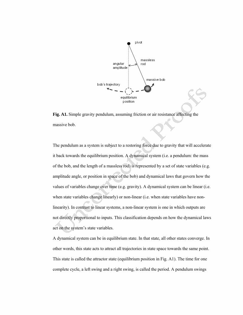
Fig. A1. Simple gravity pendulum, assuming friction or air resistance affecting the

massive bob.

The pendulum as a system is subject to a restoring force due to gravity that will accelerate

it back towards the equilibrium position. A dynamical system (i.e. a pendulum: the mass

of the bob, and the length of a massless rod) is represented by a set of state variables (e.g.

amplitude angle, or position in space of the bob) and dynamical laws that govern how the

values of variables change over time (e.g. gravity). A dynamical system can be linear (i.e.

when state variables change linearly) or non-linear (i.e. when state variables have non-

linearity). In contrast to linear systems, a non-linear system is one in which outputs are

not directly proportional to inputs. This classification depends on how the dynamical laws

act on the system’s state variables.

A dynamical system can be in equilibrium state. In that state, all other states converge. In

other words, this state acts to attract all trajectories in state space towards the same point.

This state is called the attractor state (equilibrium position in Fig. A1). The time for one

complete cycle, a left swing and a right swing, is called the period. A pendulum swings

with a specific period which depends (mainly) on its massless rod length. For example,

when released, the restoring force combined with the pendulum’s mass produces

oscillations about the equilibrium position (i.e. movements of the massive bob swinging

back and forth, over a long period of time).

Fig. A2. Point attractors representing trajectories that converge in the same equilibrium

state. (A) Direct trajectories; (B) oscillating trajectory as observed in a simple pendulum

system assuming friction or air resistance.

State variables represent the position over time of a system (e.g. the pendulum) in a

dynamical state space. The state space of the system is the set of possible values that state

variables can reach following the dynamical law or vector field in such space (e.g. the

bob’s trajectory measured in terms of angle amplitude). Consequently, a dynamical

trajectory of a system is the sequence of states generated by the action of the dynamical

law starting from some initial state.

The dynamical flow refers to the set of all dynamical trajectories through every point in

the state space (see arrows in Fig. A2). In general, those trajectories that are not stable

points are called transient dynamics towards an attractor. A picture showing all of the

qualitatively different dynamical trajectories of the system is called a phase portrait

(Strogatz, 1994). A phase portrait is a geometric representation of the trajectories of a

dynamical system in the phase plane for fixed values of parameters. Each set of initial

conditions is represented by a different curve or point.

Fig. A3. Simple gravity pendulum, assuming no friction or air resistance. The arrows

represent trajectories starting outside the attractor (circle), but ending up in a continuous

cycle along the attractor.

The combination of two different influences acting on the massive bob, one dampening

differences and another amplifying them, can create non-linearity in our example. These

influences will still create an attractor in state space since different initial positions of the

pendulum will all converge on the same periodic trajectory. These influences will create a

limit cycle: a closed, one-dimensional line of sequential points (Fig. A3).

Other basic concepts are attractor states and bifurcations. Attractor states are sets of points

that remain invariant under the dynamical law in the state space. For example, a stable

attractor has the property that all trajectories passing through all nearby states converge to

it, where the set of initial states that converge to a given attractor is termed its basin of

attraction. A basin of attraction is the set of initial conditions leading to long-term

behaviour that approaches that attractor (see Fig. A4).

Fig. A4. Schematics of three attractors in state space with trajectories leading into them.

Dotted lines represent divisions between their respective basins of attraction.

A characteristic of highly non-linear systems is that they generally have several attractors.

When considering several variables of interest describing a dynamical system, a point in

parameter space stands for a specific combination of all parameter values. Thus, the state

space is related to a fixed set of basins of attraction and attractors in the corresponding

state space of the dynamical system or phase portrait. In phase space, all possible states of

a system (or allowed combination of values of the system’s variables) are represented

with each probable state of the system corresponding to one unique point in the space

(Fig. A4).

A bifurcation occurs when a small smooth change made to the parameter values (the

bifurcation parameters) of a system causes a sudden qualitative or topological change.

Usually, bifurcations mean that the dynamical flow at one particular moment approaches

one attractor following its basin of attraction. The appearance of a border separating two

attractors is called a bifurcation. Importantly, bifurcations happen in phase space, rather

than in parameter space (Fig. A4).

In terms of small perturbations, dynamical systems can be structurally stable. This

indicates that small variations in the parameter values will produce little change in the

dynamical flow. In brief, if a perturbation does not change the topological relationship of

the flow, we say it is structurally stable. In other words, the limit sets and basins of

attraction may slightly deform and move, but the new flow will be qualitatively similar to

that before the perturbation (Demongeot, Morvan & Sene, 2008). This concept suggests

that a system can remain relatively unaltered despite small variations in its components

and relations regardless of the effects of perturbations on the structure of a system.

Consequently, the looseness involved in determining the size of a perturbation is due to

maintenance of the systemic structure.

Finally, the concept of multistability can be described as multistate dynamics (Fig. A4).

When we refer to multistability, we are usually talking about stable states or attractors; the

stability of a state depends on how quickly the system returns to a state following a

perturbation. Each state corresponds to an attractor co-existing in the phase space

associated to the activity in specific components of a system (i.e. the state variables).

Transitions between these states triggered by external perturbations can be represented in

state space by switching between two (or several) basins of attraction.

FIGURE LEGENDS

Fig. 1. Schematics of von Uexküll’s description of functional circles between the

organism and the environment (von Uexküll, 1926; von Uexküll, 1957). Adapted from

(Macinnes & Di Paolo, 2006).

Fig. 2. Ashby’s ultrastable system. E represents the essential variables. S is those

parameters that affect the sub-system R that controls the interaction with the

environment. See text for further details.

Fig. 3. Schematic representation of a closed system and its boundary. (A) The agent-

based idealization of a system. (B) The agent–environment system perspective. Dotted-

line squares represent two different notions of a system discussed herein. Schematics

based on interpretations from (Beer, 1997; Chiel & Beer, 1997; von Bertalanffy, 1968).

Fig. 4. Approaches to explaining robust and adaptive behaviour of the nervous system–

body–environment system. (A) The usual understanding of behavioural robustness in

neural systems defined as the inner-based mechanistic approach. (B) The adaptive

behaviour approach. (C) A systemic view of behavioural robustness. NN, neural

network. See main text for further details. Figures adapted and extended from (Chiel &

Beer, 1997) and (Barandiaran, 2004).

Fig. 5. Illustration of environmental influences and the effect of perturbations on inner

dynamics. In A, two environments are shown (rich and minimal media). Plots adapted

from (Freilich et al., 2010). In B, a current state of an internal control can be modified

by small or large perturbations (thick black arrows) pushing the agent–internal

dynamics within the current boundary of attraction or far from it. NN, neural network.

See main text for further details. Plot adapted from (Kitano, 2004; Kitano, 2007).

Fig. 6. Illustration of redundancy (A) and distributed robustness (B). Plots show a

hypothetical organization in which an upstream signal from the upper white circles is

processed by a number of intermediate components (dark circles) to a downstream

effector (lower white circles). Adapted from (Félix & Wagner, 2008).

Fig. 7. Schematic representation of a landscape characterized by peaks of high fitness

(z-axis) but low robustness, and others of low fitness with high neutrality (robustness).

(A) Control case. (B) After an increase in mutation rate on solutions (e.g. genotypes).

See main text for further descriptions. Figures adapted from (Burch & Chao, 2000).

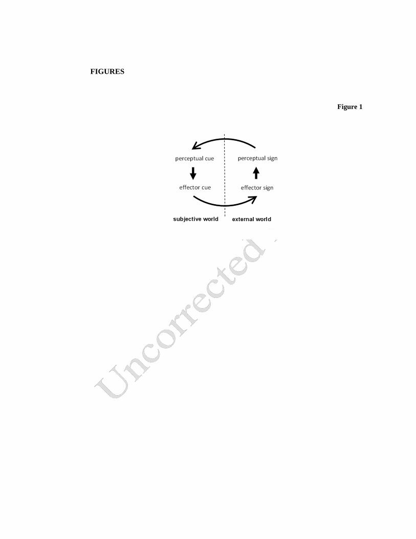
FIGURES

Figure 1

Figure 2

Figure 3

Figure 4

Figure 5

Figure 6

Figure 7