cs butxceedlineto

uld bes, New

s whom the

Downl

Journal ofApplied

Mechanics Brief NotesA Brief Note is a short paper that presents a specific solution of technical interest in mechaniwhich does not necessarily contain new general methods or results. A Brief Note should not e2500 wordsor equivalent~a typical one-column figure or table is equivalent to 250 words; a oneequation to 30 words!. Brief Notes will be subject to the usual review procedures priorpublication. After approval such Notes will be published as soon as possible. The Notes shosubmitted to the Editor of the JOURNAL OF APPLIED MECHANICS. Discussions on the Brief Noteshould be addressed to the Editorial Department, ASME International, Three Park AvenueYork, NY 10016-5990, or to the Editor of the JOURNAL OF APPLIED MECHANICS. Discussions onBrief Notes appearing in this issue will be accepted until two months after publication. Readerneed more time to prepare a Discussion should request an extension of the deadline froEditorial Department.

ie

i

a

mt

r

o

on-aselid

is

lo-r-age

outin

nee

of

thedo-

ed

n:

ularlid

per-

Plastic Localization Revisited

Maria Eugenia MaranteFaculty of Engineering, University of Los Andes, TulioFebres Cordero, Me´rida 5101, Venezuelaand Lisandro Alvarado University, Barquisimeto,Venezuela

Julio Florez-LopezUniversity of Los Andes, Tulio Febres Codero,Merida 5101, Venezuela

This brief note describes an alternative approach for the demstration of the localization criterion. In the new approach, thcriterion is not obtained in terms of the gradient jump, butterms of the plastic multiplier jump. The new demonstration issimple as the classic criterion in the loading/loading conditionbut much simpler in the loading/unloading case. It is the opinof the authors that this alternative approach is more convenifor pedagogical purposes.@DOI: 10.1115/1.1636790#

1 IntroductionThis short note does not contain new results about localizat

but a new and simpler way to present them. Specifically, this npresents an alternative procedure to demonstrate the localizcriterion. Originally, the localization analysis was expressedterms of the jump of the rate displacement gradients,@1#. Underloading conditions on both sides of the discontinuity surface,demonstration of the localization criterion has the brilliant siplicity of the classics. However, under plastic-loading/elasunloading conditions, the demonstration is complicated,@2#.

In Ref. @3#, localization is analyzed by carrying out a spectanalysis of the characteristic tensor and explicit analytical resfor the critical bifurcation directions and the corresponding haening modulus were obtained. Reference@4# also deals, as in@2#,with localization in the case when the material follows differeconstitutive branches in the band and the material outside.

In this short paper, it is shown that the localization conditi

Contributed by the Applied Mechanics Division of THE AMERICAN SOCIETY OFMECHANICAL ENGINEERSfor publication in the ASME JOURNAL OF APPLIED ME-CHANICS. Manuscript received by the ASME Applied Mechanics Division, July 12002, final revision, June 4, 2003. Associate Editor: E. Arruda.

Copyright © 2Journal of Applied Mechanics

oaded 18 Dec 2009 to 137.229.21.11. Redistribution subject to ASME li

on-einass,onnt

on,otetionin

the-

ic-

alultsrd-

nt

n

expressed in terms of the plastic multiplier jump can be demstrated in a very simple way, as simple as the loading/loading cof the Rudnicki and Rice demonstration, but that is equally vafor the loading/unloading case.

It is the opinion of the authors that this alternative approachmore convenient for pedagogical purposes.

Finally, the framework chosen for the demonstration of thecalization criterion is the one of plasticity. However, it is impotant to underline that the same procedure can be used in dammechanics. For instance, in the case of brittle behavior withsignificant plasticity, the localization criterion can be expressedterms of the damage jump~or the damage multiplier jump! insteadof the gradient jump. On the other hand, the use of only oplastic multiplier limits the validity of the demonstration to thcase of smooth yield surfaces.

2 A Plasticity ModelLet us consider a plasticity model within the framework

infinitesimal strains. The elasticity law is given by

s i j 5Si jkl ~«kl2«klp ! (1)

whereS is the elasticity tensor with the usual symmetries andremaining symbols in~1! have the conventional meaning. A yielfunction f 5 f (s i j ,ak)<0 is introduced to describe the elastic dmain in the usual way. The internal variablesak are hardening~orsoftening! parameters. The plastic strain evolution law is obtainfrom a plastic potentialg5g(s i j ,ak) in the customary way:

« i jp 5l

]g

]s i j; l>0. (2)

The plastic multiplier is computed via the consistency conditio

H l50 if f ,0 or f ,0

l.0 if f 50 and f 50.(3)

Finally, the internal variable evolution laws are written as

ak5lhk~s,a!. (4)

3 The Classic Localization Analysis of Rudnicki andRice

The localization analysis consists in the search of a partickind of solutions with strain rate discontinuities. Consider a sowith a discontinuity surface of normaln. The values of the vari-ables in one side of the discontinuity are denoted by the suscript 1 and on the other side by the superscript2. The jump of

1,

004 by ASME MARCH 2004, Vol. 71 Õ 283

cense or copyright; see http://www.asme.org/terms/Terms_Use.cfm

a

n

t

n

t

e

ionsth-wce,

ewm-ul-

ides

, are

the

c-tive

-on-

allioned

s ofng/

a-larn

ss

Downl

any variableX is denoted byiXi5X12X2. The Maxwell com-patibility condition and the equilibrium across the surfacewritten as

i « i j i51

2~nipj1nj pi !; is i j inj50 (5)

wherep is the jump of the normal derivative of the displacemerate. Let us assume that plasticity is active in both sides ofsurface, i.e.,l1.0 andl2.0. Then, the jump of the stress rais given by

is i j i5Si jkl i «kli2iliSi jkl

]g

]skl. (6)

The consistency condition and the internal variable evolution lalead to

i f i5] f

]s i jis i j i1

] f

]a ihi ili50. (7)

The combination of~6! and~5! on one hand and~7! and~5! on theother gives

~Si jkl njnk!pl2S Si jkl

]g

]sklnj D ili50 (8a)

S ] f

]s i jSi jkl nkD p12S ] f

]s i jSi jkl

]g

]skl2

] f

]a ihi D ili50. (8b)

The classic localization analysis is carried out by computingmultiplier jump from ~8b! and introducing it in~8a!, then theexpression that defines the gradient jumpp is obtained:

~Ki jkl njnk!pl50; (9)

where

Ki jkl 5Si jkl 21

ASi jab

]g

]sab

] f

]scdScdkl ;

A5] f

]s i jSi jkl

]g

]skl2

] f

]a ihi . (10)

Now, localization under the aforementioned conditions is opossible if the matrixKi jkl njnk is singular.

4 Classic Localization Analysis in Terms of the PlasticMultiplier

It can be immediately noticed that an alternative criterion cbe obtained in terms of the multiplier jumpili instead of thegradient jumpp. The expression of the gradient jump from~8a! is

pl5~Si jkl nknj !21Bi ili ; where Bi5Si jkl

]g

]sklnj . (11)

Notice that the matrixSi jkl nknj is always invertible. Now intro-ducing ~11! into ~8b! gives

Cili50; where C5A2] f

]s i jSi jkl nk~Scbalnanb!21Bc .

(12)

Therefore, localization is only possible ifC is equal to zero. Oth-erwise, the multiplier jump must be equal to zero and so musthe gradient jumpp. The conditions

C50 and det~Ki jkl njnk!50 (13)

must, of course, be equivalent.A similar result to~13a! can also be obtained from the analys

of the problem in terms of the jump of the rate displacemgradients~that is as in the previous section! by the computation ofa critical hardening modulus for localization~see@5#!.

284 Õ Vol. 71, MARCH 2004

oaded 18 Dec 2009 to 137.229.21.11. Redistribution subject to ASME li

re

tsthee

ws

the

ly

an

be

isnt

Localization Analysis Under the LoadingÕUnloadingCondition

The preceding localization analyses assumed loading conditon both sides of the discontinuity surface. However, the hypoesis l1.0 and l2.0 was never verified. Let us assume nothat localization occurs with loading on one side of the surfasay the positive side, and unloading on the other side; i.e.,l1

.0 andl250.The demonstration of the localization criterion, under these n

conditions, using the Rudnicki and Rice approach is more coplicated. On the other hand, the generalization of the plastic mtiplier approach is almost immediate. The stress rate on both sof the discontinuity surface can be written as follows:

s i j15Si jkl «kl

1 2 l1Si jkl

]g

]skl; s i j

25Si jkl «kl2 . (14)

That is

Ûs i j Û5Si jkl Û «klÛ2l1Si jkl

]g

]skl. (15)

The consistency conditions, also on both sides of the surface

f 15] f

]s i js i j

11] f

]a ihil

150; f 25] f

]s i js i j

2,0 (16)

therefore

i f i5] f

]s i jis i j i1

] f

]a ihil

1.0. (17)

The combination of~5! and~15! and the combination of~17! nowleads to

H ~Si jkl njnk!pl1S Si jkl

]g

]sklnj Dl150

S ] f

]s i jSi jkl nkD pl2S ] f

]s i jSi jkl

]g

]skl2

] f

]a ihi Dl1.0.

(18)

The jump gradientp can be expressed again as a function ofplastic multiplierl1:

pl5~Si jkl nknj !21Bil

1 (19)

and the inequality~18b! becomes

Cl1,0 (20)

whereC and Bi have the expression given in the previous setions. On the the other hand the plastic multiplier must be posil1.0. Thus, localization is only possible if

C<0. (21)

It can be seen that the condition~21! includes both cases: localization under the loading/loading and the loading/unloading cditions.

As indicated in the Introduction this is not a new result atbut a simpler way to obtain the mathematical proof of localizatconditions under loading/unloading conditions. It can be indenoticed that with this alternative approach the demonstrationlocalization conditions in cases, loading/loading and loadiunloading, are equally simple.

6. ExampleThe termC does not correspond to the determinant of the m

trix Ki jkl njnk. This can be observed by considering a particucase. For instance, letS be the isotropic elasticity tensor written iterms of the elastic modulusE and the Poisson coefficientn. Theyield function f is expressed as a function of the Von Mises streseq as follows:

Transactions of the ASME

cense or copyright; see http://www.asme.org/terms/Terms_Use.cfm

ta

oli

t

r

e

n

ue

ut

the

c-de,nalhe-nof

ca-ndon

a-

isitho-

ef-

cellits

ller

eralys-ss a

ee-tric/

third,. Offectofolid

test isala-

edored all

tionow,the

heiondedundns.f theergeeetsix

m

Downl

f 5seq2syS 12a

acrD (22)

wheresy andacr are material parameters. The functiong is takenequal tof andh is equal to one. Let us consider a uniaxial strecondition. The determinant ofKi jkl njnk is now

det~Ki jkl njnk!51

2

~~12nl !2Eacr2sy!E2

~Eacr2sy1syn2!~11n!

(23)

and the value ofC is

C5~12nl !

2Eacr2sy

acr. (24)

It can be noticed that although the termC is not identical todet(ki jkl njnk), both quantities become zero or negative undersame conditions. Under plane stress conditions both criteriadiffers but given the same value of the vectorn too.

AcknowledgmentThe results presented in this paper were obtained in the co

of an investigation sponsored by FONACIT, CDCHT-ULA, anCDCHT-UCLA.

References@1# Rudnicki, J. W., and Rice, J. R., 1975, ‘‘Condition for the Localization

Deformation in Pressure-Sensitive Dilatant Materials,’’ J. Mech. Phys. So23, pp. 371–394.

@2# Rice, J. R., and Rudnicki, J. W., 1980, ‘‘A Note on Some Features ofTheory of Localization of Deformation,’’ Int. J. Solids Struct.,16, pp. 597–605.

@3# Ottosen, N. S., and Runeson, K., 1991, ‘‘Properties of Discontinuous Bifution Solutions in Elasto-Plasticity,’’ Int. J. Solids Struct.,27, pp. 401–421.

@4# Chambon, J., 1986, ‘‘Bifurcation Par Localisation en Bande de CisaillemUne Approache Avec des Lois Incrementalment Non Line´aires,’’ J. Mec.Theor. Appl.,5, pp. 277–298.

@5# Rice, J. R., 1976, ‘‘The Localization of Plastic Deformation,’’Theoretical andApplied Mechanics, W.T. Koiter, ed., North-Holland, Amsterdam.

The Three-Dimensional Analog of theClassical Two-Dimensional TrussSystem

Richard M. ChristensenLawrence Livermore National Laboratory, University ofCalifornia, P.O. Box 808 L-356, Livermore,CA 94551-9900 and Stanford University,Stanford, CA 94305, Hon. Mem. ASME

The octet-truss lattice system of Fuller and examined by Depande, Fleck and Ashby is here reasoned to be the most fumental form for a three-dimensional truss system, placing it asthree-dimensional analog of the classical two-dimensional trsystem. Useful applications may be possible from nanomscales up to space station scales, in addition to the usual scaleinterest in materials science.@DOI: 10.1115/1.1651090#

The octet-truss lattice system based upon the patent of F@1#, describes an open cell, low-density material or structuresustains loads by the direct axial deformation of the mate

Contributed by the Applied Mechanics Division of THE AMERICAN SOCIETY OFMECHANICAL ENGINEERSfor publication in the ASME JOURNAL OF APPLIED ME-CHANICS. Manuscript received by the ASME Applied Mechanics Division, Septeber 25, 2002; final revision, September 19, 2003. Associate Editor: E. Arruda.

Copyright © 2Journal of Applied Mechanics

oaded 18 Dec 2009 to 137.229.21.11. Redistribution subject to ASME li

ss

helso

ursed

fds,

he

ca-

nt,

sh-da-

thessters of

llerhatrial

members. Most low-density material forms support loads byfar less efficient bending mechanism, Roberts and Garboczi@2#.Wicks and Hutchinson@3# have shown that the efficient truss ation can be profitably employed in a plate form. DeshpanFleck, and Ashby@4# have modeled and tested a three-dimensiocellular material which is based upon the tetrahedral and octadral cells of Fuller@1# giving a truss effect. This truss-type actiowill now be elaborated, beginning with the much simpler casethe classical two-dimensional truss system.

The two-dimensional truss system is ubiquitous in its applitions. With members arranged in triangular form, it resists asustains loads through the ‘‘direct’’ action of the axial deformatiof its members. A continuous system of equilateral triangular mterial cells has an effective or average Young’s modulus,E,~Christensen@5# and Gibson and Ashby@6#!, given by

E51

3cmEm

whereEm is the material Young’s modulus andcm is the volume~area! fraction of the material relative to the total volume. Thdirect resistance behavior for triangular cells is in contrast wthat which occurs with the behavior for two-dimensional hexagnal ~honeycomb! cells. The system of hexagonal cells has anfective Young’s modulus given by@5,6#

E53

2cm

3 Em .

Although both forms are isotropic in the plane, the hexagonalform resists loads by the bending action of its members, andeffective Young’s modulus can be orders of magnitude smathan that for the triangular truss form forcm

3 !cm which is theassumed and normal range of application. Thus the equilattriangular form provides the basic and highly efficient truss stem for two-dimensional applications. It is difficult to pinpoint itorigins, but it has been used for multitudes of centuries and aclassical concept, it ranks very highly. Now the basis for the thrdimensional truss system will be discussed by taking a geomesymmetry approach.

There are five platonic solids~polyhedra!: the tetrahedron,cube, octahedron, dodecahedron, and isocahedron. The first,and fifth of these have faces defined by equilateral trianglesthese three, there is only one known form that admits a perspace-filling type of packing. This is a particular combinationtetrahedral and octahedral solids. Thus, of the five regular sforms, there are only two known methods of filling space:~i! theobvious case of the packing of cubes and~ii ! the far from obviouscase of tetrahedra plus octahedra. Case~i! with material membersin simple cubical form is of no interest here, since in some stait only resists shear deformation by a bending mechanism. Icase~ii ! that will now be used to develop the three-dimensiontype of truss system involving only the direct mechanism of mterial resistance.

The unit cell is shown in Fig. 1 with a tetrahedron inscribinside a guiding cube in the manner shown. Next, three mcubes are arranged in the same 1–3 plane as that in Fig. 1 anwith a common vertex~node! at the coordinate origin for theinscribed tetrahedra. These four cubical forms have reflecsymmetry across each of their common planar interfaces. Nfour more cubes with inscribed tetrahedrons are placed abovefirst four, with a form prescribed by reflection symmetry about tcommon plane of the two groups of four cubes. This constructnow contains one complete octahedron in the center, surrounby eight tetrahedrons, and with parts of other octahedrons arothe periphery. This form is then extended in all three directioEach face of a tetrahedron or octahedron mates with a face oother. The edges of two tetrahedrons and two octahedrons mto form a common edge. Eight tetrahedra and six octahedra mat a node. Emanating from a node are 12 common edges in-

004 by ASME MARCH 2004, Vol. 71 Õ 285

cense or copyright; see http://www.asme.org/terms/Terms_Use.cfm

rg

k

t

hit

g

n

1ate

s in

tioe innit

on-ightdi-utisn-xialinof

russve

the

try

ed,d by

. Inee-em.e-te-thelar,

theana-estectweenom-

Downl

directions. The overall region contains tetrahedra and octaheda 2:1 ratio, and is completely space filling. The common edwill now be interpreted as material members giving an open cperiodic system with material members of identical size. Thedifference between the classical two-dimensional truss andthree-dimensional truss is that six material members meet ainterior node in two dimensions whereas in three dimensionsmembers join at a node. As shown, the entire structure is builfrom the tetrahedral unit cell.

Now, the mechanical properties problem can be approacThe tetrahedral unit cell in Fig. 1 is subjected to deformatmodes of uniaxial extension, shear, and dilatation. The resuleffective mechanical properties have cubic symmetry withE115E225E33, y125y235y31, and m125m235m31 for the Young’smoduli, Poisson’s ratio’s, and shear moduli. These propertiesanalytically determined as

E11

Em5

2&

3

A

L2 51

9cm

y1251

3

m12

Em5

1

&

A

L2 51

12cm

k

Em5

2&

3

A

L2 51

9cm

whereA is the area of the material member,L its length,cm the~small! material volume fraction, andk is the effective bulkmodulus. All of the cubic properties are seen to involve the ecient, direct mechanism of deformation as opposed to bendHaving cubic symmetry, these results are not isotropic. The deof anisotropy can be easily established. Take axis 18 in a directionmaking equal angles with the axes 1, 2, and 3 in Fig. 1. The te

Fig. 1 Tetrahedral unit cell

286 Õ Vol. 71, MARCH 2004

oaded 18 Dec 2009 to 137.229.21.11. Redistribution subject to ASME li

a ines

ell,eythist an12up

ed.oning

are

ffi-ing.ree

sor

transformation relation relating the uniaxial compliance in the8direction to the compliance properties in the 1, 2, 3 coordinsystem is

S11118 51

3~S111112S112212S1212!.

Using this relation and the above results, the Young’s moduluthe 18 direction is found to be

E118

Em5

1

5cm .

Thus, the maximum to minimum Young’s moduli are in a 9:5 rawhich is not extreme and could even be used to advantagparticular problems. All of these results from the tetrahedral ucell are consistent with those of Deshpande, Fleck, and Ashby@4#,obtained from an octahedral unit cell.

A model of this three-dimensional truss system has been cstructed as shown in Fig. 2. The model is composed of the etetrahedral unit cells previously discussed. It consists of 36 invidual material members with a material volume fraction of aboone half of 1%. One of the square ‘‘waists’’ of the octahedronvisible in the center of the model. The model physically demostrates that the resistance to deformation is by the direct adeformation mechanism. It has very high structural rigidity,shear as well as in dilatation. The form in Fig. 2 is an examplea free-standing structure specified by this three-dimensional tsystem. A different view of the Fig. 2 structure shows it to hathe general shape of a cube with nodes at the corners andcenters of the faces~face-centered cubic!, but with none of thematerial members having the directions of the cubical symmeaxes. This generic structural unit could have wide utility.

Many three-dimensional truss type forms can be visualizsuch as one with hexagonal symmetry, but the one developeFuller @1# and analyzed by Deshpande, Fleck, and Ashby@2# islikely to be the simplest in concept, analysis and constructionfact, it is here argued that this truss system is the logical thrdimensional analog of the classical two-dimensional truss systThe basis for this assertion is the following. This thredimensional truss form involving the direct mechanism for marial resistance is the only system that can be derived fromgeometrically basic, platonic solids, as shown above. In particuthe unit cell for the analysis of mechanical effects is that ofsingle tetrahedron. The tetrahedron is the three-dimensionallog of the equilateral triangle. The tetrahedron is the simplthree-dimensional form that gains structural integrity by the dirresistence mechanism of its material members. These ties bettwo-dimensional and three-dimensional features are at a cpletely fundamental level of mechanical behavior and effect.

Fig. 2 Eight tetrahedral cells, 36 material members model

Transactions of the ASME

cense or copyright; see http://www.asme.org/terms/Terms_Use.cfm

e

i.s

v

Dc

i

t

o

c

o

t

h

llylv-

the. As

d to

lic

tact

adeator.rmo-nary

alf-l of

re

ies,

-tan-

ends

Downl

Interesting applications could occur at all scales, up to vlarge scales. For example, orbital space structures place amium upon a three-dimensional form that maximizes volumeminimum weight while preserving high structural rigidity. Thisa prescription for a modular three-dimensional truss systemthe other end of the scale, nano-engineering techniques mayday be used to assemble the present three-dimensional trussusing individual rigid molecules such as nanotubes to have asmall, very rigid building block essentially based upon the tethedral unit cell.

This work was performed under the auspices of the U.S.partment of Energy by the University of California, LawrenLivermore National Laboratory under Contract No. W-7405-En48. This work was supported by the Office of Naval Research,Y. D. S. Rajapakse, program manager.

References@1# Fuller, R. B., 1961, ‘‘Octet Truss,’’ U.S. Patent Serial No. 2, 986, 241.@2# Roberts, A. P., and Garboczi, E. J., 2002, ‘‘Elastic Properties of Model R

dom Three-Dimensional Open-Cell Solids,’’ J. Mech. Phys. Solids,50, pp.33–55.

@3# Wicks, N., and Hutchinson, J. W., 2001, ‘‘Optimal Truss Plates,’’ Int. J. SolStruct.,38, pp. 5165–5183.

@4# Deshpande, V. S., Fleck, N. A., and Ashby, M. F., 2001, ‘‘Effective Properof the Octet-Truss Lattice Material,’’ J. Mech. Phys. Solids,49, pp. 1747–1769.

@5# Christensen, R. M., 2000, ‘‘Mechanics of Cellular and Other Low-DensMaterials,’’ Int. J. Solids Struct.,37, pp. 93–104.

@6# Gibson, L. J., and Ashby, M. F., 1997,Cellular Solids: Structure and Proper-ties, 2nd Ed., Cambridge Univ. Press, Cambridge, UK.

Contact Problem Involving FrictionalHeating for Rough Half-Space

Volodymyr Pauk1

Institute of Mechanics and Applied Informatics,Technische Universita¨t Dresden, Dresden D-01062,Germany

Plane contact problem of a punch sliding over a half-spaceconsidered. The surface of the half-space is assumed to be rand the roughness heights have the Gaussian distribution.heat generation due to the friction is taken into account. Tproblem is reduced to nonlinear integral equations which asolved approximately. The effects of the frictional heating androughness on the contact size and on the contact pressurepresented. @DOI: 10.1115/1.1687793#

1 IntroductionWhen two bodies are in the sliding contact with a dry frictio

the heat is generated between them and the produced thermotic deformation may have a significant effect on the tribologibehavior of the contacting materials. The solutions of this kindproblems can be found in many papers. The plane problem inving the stationary heat generation for a half-space is first conered in@1,2#. The solution is obtained under assumption thatcontacting surfaces are perfectly smooth. However, the real eneering surfaces are covered with microscopic roughness. Tare many approaches modelling the surface roughness and sing its effect on the normal contact. The well-known GreenwooWilliamson @3# method treats the roughness as spherical asper

Contributed by the Applied Mechanics Division of THE AMERICAN SOCIETY OFMECHANICAL ENGINEERSfor publication in the ASME JOURNAL OF APPLIED ME-CHANICS. Manuscript received by the ASME Applied Mechanics Division, Feb.2003, final revision, Sept. 30, 2003. Associate Editor: J. R. Barber.

Journal of Applied Mechanics

oaded 18 Dec 2009 to 137.229.21.11. Redistribution subject to ASME li

rypre-forsAtomeformeryra-

e-eg-Dr.

an-

ds

ies

ity

isugh

Theheretheare

n,elas-aloflv-

sid-hengi-ere

tudy-d-

ities

of uniform radius and random heights distributed over nominaflat surface. The plane normal contact of rough cylinders invoing this model is presented in@4#.

The aim of this contribution is to study the phenomenon ofheat generation due to the friction between the rough surfacesa model of roughness, the Greenwood-Williamson~G-W! ap-proach is used and the frictional heating process is considerebe stationary. The method of solution is similar to that used in@4#for the normal contact of rough elastic bodies.

2 Problem Formulation and Integral EquationsLet us consider the following contact problem. A parabo

punch is pressed by the normal loadP and slides inz-directionwith the constant velocityV over a half-space~Fig. 1!. Frictionforces due to the sliding punch produce the heat in the conarea (2a,a) and the heat source

q~x!52Vsyz~x!5 f Vp~x!, uxu,a (1)

~f is the friction coefficient,p(x) is the contact pressure,syz is thefriction force! flows into the half-space because the punch is mof poor conductive material and can be considered as an insulFree boundaries of the half-space are assumed to be also theinsulated. The heat generation process is considered as statioand plane.

We assume that the punch surface is smooth while the hspace one is covered with microscopic asperities. The moderoughness is that proposed by Greenwood-Williamson@3#. Thereader can find the details for this model in@3# or in the Johnson’sbook, @5#. According to the G-W model, the effective pressubetween rough surfaces is calculated as

p~x!5lhEu~x!

`

@ t2u~x!#3/2f~ t !dt (2)

where l54/3EAB, 1/E5(12n12)/E11(12n2

2)/E2 , Ei , n i areYoung’s coefficients and Poison’s ratios of the contacting bodB is the constant radius of spherical asperities,u(x) is the nominaldistance between the punch and the half-space,h is the density ofasperities, andf~•! is the probability density function of the asperity height distribution, assumed to be Gaussian with the sdard derivations

f~ t !51

sA2pexpS 2

t2

2s2D . (3)

The nominal separation between the contacting bodies depon the punch radiusR, elastic~due to the normal pressurep(x),see@5#! and thermal~due to the heat source~1!, see@1#! displace-ments. It can be calculated as

4,

Fig. 1 Contact geometry

MARCH 2004, Vol. 71 Õ 287

cense or copyright; see http://www.asme.org/terms/Terms_Use.cfm

a

hea

st

T

s

d

ionver-

f

e the

res-

be-er-

Downl

u~x!5d1x2

2R2

2

pE E2a

a

p~s!lnUs2x

s Uds

2f Va1~11n1!

2K1E

2a

a

p~s!us2xuds (4)

whered is the separation atx50, a1 , K1 are, respectively, thethermal expansion coefficients and the conductivity for the hspace.

The Eqs.~2!, ~4! are the system of integral equations for tproblem solution. It is convenient to rewrite it in the normalizform. Introducing dimensionless variables, functions and pareters

r 5x

A2Rs, j5

s

A2Rs, d* 5

d

s, c5

a

A2Rs,

k5p f Va1~11n1!EA2Rs

4K1,

(5)

d58

3

hsARB

pAp, u* ~r !5

u~x!

s, p* ~r !5

A8R/s

pEp~x!,

t5t

s

we obtain the system of integral equations

u* ~r !5d* 1r 22E2c

c

p* ~j!H lnUj2r

j U1kuj2r uJ dj (6)

p* ~r !5dEu* ~r !

`

@t2u* ~r !#3/2 exp~2t2/2!dt. (7)

Now we need the presentation for the effective contact preswithin the contact nominal area. Numerical results for the conof rough surfaces,@6#, shown that the effective pressure has a bshape with the zero derivative at the contact area edges.shape, which is due to the Gaussian distribution of aspeheights, can be approximated by the following expression:

p* ~r !5p* ~0!F12r 2

c2G 2

, ur u<c (8)

wherep* (0) andc are unknown maximum of the contact presure and normalized contact size. Note that the similar presetion for the effective contact pressure is used in the corresponelastic problem,@4#.

Substituting the presentation~8! into ~6! we obtain the newform for the Eq.~6!:

u* ~r !5d* 1r 22p* ~0!@c f1~r /c!1kc2f 2~r /c!# (9)

where we have denoted

f 1~z!5E21

1

@12t2#2 lnUt2z

t Udt

51

15@3z5210z3115z18# lnu11zu

11

15@3z5110z3215z18# lnu12zu

11

15@18z226z4#

(10)

f 2~z!5E21

1

@12t2#2ut2zudt51

15@z625z4115z215#.

288 Õ Vol. 71, MARCH 2004

oaded 18 Dec 2009 to 137.229.21.11. Redistribution subject to ASME li

lf-

edm-

ureactellhis

rity

-nta-ing

3 Calculation and ResultsThe main difficulty in the solution of Eqs.~7!, ~9! is their non-

linearity. However, the approximate method of the calculatproposed in@4# and used here gives a good accuracy and congence. It consists of the following steps:

1. For givenp* (0) the distanced* 5u* (0) is calculated fromEq. ~7! at r 50, i.e.,

p* ~0!5dEd*

`

@t2d* #3/2 exp~2t2/2!dt. (11)

The method of trial and error is used.

2. Assuming

p* ~r !50.5p* ~0!, (12)

we can solve the Eq.~7! by trial and error and find the value ofu*as a function ofp* (0), which corresponds to this assumption.

3. For these values ofu* and p* (0), and r 50.541c ~whatcorresponds to the assumption~12!, see Eq.~8!!, the contact sizec is calculated as a positive solution of the quadratic Eq.~9!.Notice here that this step is different than that proposed in@4#.

4. For known values ofc andp* (0) we can calculate the load

P* 52P

pEs5

2

pEs E2a

a

p~x!dx516

15cp* ~0!, (13)

the functionu* (r ) ~9!, and, finally, by a numerical integration o~7!, the contact pressure distributionp* (r ).

Of course, the described procedure is approximate becausassumption~12! is used. However, it was shown in@4# that thecalculation error for the contact sizec due to this assumption issmall~,2%!. In addition, similarly to the method proposed in@4#,we have compared the distributions of the effective contact psure obtained from the formulas~8! and ~7! where the functionu* (r ) is already known. We can conclude that the differencetween these distributions is very small also in the case of thmoelastic problem. By this way, the choice of the presentation~8!for the contact pressure is confirmed.

Fig. 2 Contact size and maximal normal pressure as functionsof load P* for dÄ0.3 and some values of k

Transactions of the ASME

cense or copyright; see http://www.asme.org/terms/Terms_Use.cfm

cs

g

-n-d

size

fre

Downl

The aim of numerical calculation is to study the effect of fritional heating on the contact area size and on the contact predistribution.

Figure 2 shows the maximal contact pressurep* (0) and thecontact sizec as functions of the loadP* for some values of thefrictional heating ratiok. We see that for the isothermal cas~k50! as well as for small values ofk ~k,2! the contact area sizec increases when the loadP* grows. When the frictional heatingis high ~k>2! we observe a significantly different tendencnamely, the contact path shrinks if the load increases. Simuneously, the maximum of the contact pressurep* (0) grows. Thisgrowth is especially significant for the high frictional heatinPhysically this tendency means that for small values ofk, theelastic deformation has the main effect on the solution whilethermal distortion dominates for high values ofk.

Figures 3~a,b! show the effect of the frictional heating on th

Fig. 3 „a… Load P* as function of parameter k for p * „0…Ä0.1and some values of d; „b… contact size c as function of param-eter k for p * „0…Ä0.1 and some values of d

Journal of Applied Mechanics

oaded 18 Dec 2009 to 137.229.21.11. Redistribution subject to ASME li

-sure

e

y,lta-

.

the

e

load P* and on the contact sizec for some values of the roughness parameterd under assumption that the maximum of the cotact pressure is fixedp* (0)50.1. We see that to obtain this fixepressure maximum, the smaller loadP* must be applied when thefrictional heating increases. In the same time, the contact areac decreases.

The distributions of the contact pressurep* (r ) is shown inFigs. 4~a,b! for two values of the loadP* and for some values othe ratio k. Significant effects due to the frictional heating aobserved.

Fig. 4 „a… Distribution of contact pressure for dÄ0.3, P*Ä0.05 and some values of k; „b… distribution of contact pres-sure for dÄ0.3, P*Ä0.1 and some values of k

MARCH 2004, Vol. 71 Õ 289

cense or copyright; see http://www.asme.org/terms/Terms_Use.cfm

n

r

l

i

sa

e

uc-l is

turegi-theinto

e-s. 1.are

ionequi-a-itu-plesA

the

ach

e

th.

l

ossach

com-

thethe

en-e

cial

tedual

heir

uluscialThissignctlymal

1

Downl

4 ConclusionsThe contact problem involving simultaneously the surfa

roughness and the heat generation due to the friction is conered. The essential difference between pure elastic contactthat involving the frictional heating was observed. The presenstudy can be considered as a model for the investigation oftribological behavior of the real contact, which occurs frequenin many engineering systems, particularly in brakes, during griing and cutting processes.

AcknowledgmentsThe author is pleased to acknowledge the support from

Alexander von Humboldt Foundation~Germany! permitting hisvisit at Technische Universita¨t Dresden.

References@1# Korovchinskii, M. V., 1965, ‘‘Plane Contact Problem of Thermoelacticity Du

ing Quasi-Stationary Heat Generation on the Contact Surfaces,’’ Trans. AS87, pp. 811–817.

@2# Barber, J. R., 1976, ‘‘Some Thermoelastic Contact Problems Involving Ftional Heating,’’ Q. J. Mech. Appl. Math.,29, pp. 1–13.

@3# Greenwood, J. A., and Williamson, J. B. P., 1966, ‘‘Contact of Nominally FSurfaces,’’ Proc. R. Soc. London, Ser. A,A295, pp. 300–319.

@4# Lo, C. C., 1969, ‘‘Elastic Contact of Rough Cylinders,’’ Int. J. Mech. Sci.,11,pp. 105–115.

@5# Johnson, K. L., 1987,Contact Mechanics, Cambridge University Press, Cambridge, UK.

@6# Greenwood, J. A., and Tripp, J. H., 1967, ‘‘The Elastic Contact of RouSpheres,’’ ASME J. Appl. Mech.,34, pp. 153–159.

Peeling in Bimaterial Beams: ThePeeling Moment and Its Relation to theDifferential Rigidity

Thomas D. MooreAnalog Devices B.V., Raheen Business Park, Limerick,Ireland and Thermomechanical Solutions,Limerick, Irelande-mail: tmoore@thermomechanical.com

John L. JarvisDepartment of Mechanical and Aeronautical EngineerinUniversity of Limerick, Limerick, Irelande-mail: john.jarvis@ul.ie

Two-layer beams (i.e., bimaterials) under thermomechanstress are prone to peeling or delamination at the free edges.self-equilibrating peeling stress gives rise to a peeling momM p close to the free ends. A simple and exact formula for Mp ispresented in which the sign of Mp indicates whether the beam iprone or resistant to delamination. The effect on both the signmagnitude of Mp of the flexural rigidities of both layers is examined. As the stiffness of one layer becomes dominant, the matude of the differential rigidity converges to one-half the thicknof the opposite layer.@DOI: 10.1115/1.1651092#

1 Bending Moments in a Bimaterial BeamA review of prior work is provided in@1#. This present analysis

of bending in a bimaterial beam uses the work of Timoshenko@2#

Contributed by the Applied Mechanics Division of THE AMERICAN SOCIETY OFMECHANICAL ENGINEERSfor publication in the ASME JOURNAL OF APPLIED ME-CHANICS. Manuscript received by the ASME Applied Mechanics Division, April 22003; final revision, September 19, 2003. Associate Editor: M.-J. Pindera.

290 Õ Vol. 71, MARCH 2004 Copyright © 2

oaded 18 Dec 2009 to 137.229.21.11. Redistribution subject to ASME li

cesid-andtedthetlyd-

the

r-ME,

ic-

at

-

gh

g,

calTheent

nd-gni-ss

as its foundation. It is convenient to use that work as an introdtion, and in this section a brief summary of the relevant materiamade.

When a bimaterial beam is subject to a change in temperathe two layers in general expand at different rates, but the lontudinal displacement at the interface must be identical becauselayers are bonded together. Thus interfacial shear forces comeplay to enforce the condition of identical longitudinal displacments. Within each layer, equal and opposite longitudinal forceParise in reaction to the interfacial shear forces, as shown in FigThese forces acting through the neutral axes of the layersstatically equivalent representations of the longitudinal reactstresses that actually arise. They are necessary to maintainlibrium of each layer in the longitudinal direction. The combintion of the interfacial shear force and the offset reaction longdinal force within each layer generates the shear-induced couM1 and M2 shown in Fig. 1 which cause each layer to bend.representative portion of the bimaterial beam remote fromends is shown in Fig. 1.

Because the layers are bonded, the interfacial curvature of elayer must also be identical. Timoshenko@2# derived the followingformula for the radius of curvature of the interface:

1

r5

~a22a1!~ t2t0!

h11h2

21

2~E1I 11E2I 2!

h11h2F 1

E1h11

1

E2h2G (1)

where h1 and h2 are the beam thicknesses,a1 and a2 are thecoefficients of thermal expansion~CTE!, E1 and E2 are themoduli of elasticity,I 1 and I 2 are the moments of inertia of thupper and lower layer about their respective centroids, andt andt0 are the final and initial temperatures of the beam of unit wid

Timoshenko also showed that the longitudinal forcesP1 andP2are equal in magnitude so they were replaced with the symboP.The magnitude ofP in a beam of unit width was given by

P52~E1I 11E2I 2!

~h11h2!r. (2)

He analyzed the distribution of stresses in an arbitrary crsection remote from the ends as in Fig. 1, and stated that for elayer the longitudinal stresses can be expressed as a linearbination of a central forceP, and a coupleM1 or M2 .

Timoshenko then turned his attention to the stresses nearends of the beam. He examined the particular case whereYoung’s modulus as well as the thickness of each layer were idtical, i.e.,E15E2 andh15h2 . This latter condition meant that thmoment of inertia of each layer was also identical viz.I 15I 2 .Also sinceh15h2 , the offset~i.e., the lever arm of the moment!for each layer were identical, and thusM15M2 . Under theseconditions (E, I and M of each material identical! the shear-induced moments were sufficient to produce identical interfacurvatures for each layer.

Timoshenko acknowledged that in the general caseE1I 1 is notequal toE2I 2 and the momentsM1 andM2 acting alone will notbe sufficient to cause identical interfacial curvatures. He stathat the peeling stress distribution could be reduced to two eqand opposite couples of such magnitude as to produce~with theshear-induced couples previously considered! equal curvatures 1/rat the interface.

In the following section these couples are examined and tmagnitude and sign are determined.

2 Peeling or Pinching Stresses at the Free EdgeConsidering the more general case where the Young’s mod

and the thickness of each layer is different, then an interfanormal stress exists close to the free ends as shown in Fig. 2.normal stress is self-equilibrating, and consequently reversesso that the normal forces arising from the positive area exaoffset those produced by the negative area. In Fig. 2 the nor,

004 by ASME Transactions of the ASME

cense or copyright; see http://www.asme.org/terms/Terms_Use.cfm

.

t

f

n

h

s

-

reing

not

l

ma-the

.

of

sibly

sec-e-

lwiths

s 10

d

isthe

ssand

for a

Downl

stress is shown tensile~i.e., peeling! at the free edge and compressive inboard, although as fully discussed in@1# the opposite canoccur depending on layer geometries and material properties

In order for identical interfacial curvatures to be produced thconsidering Figs. 1 and 2 the following equation must be satisfi@1#:

M12M p

E1I 15

1

r5

M21M p

E2I 2. (3)

Reordering yields an expression for the coupleM p that arisesfrom the normal stress. This can be written as

M p5h1h2~h2

2E22h12E1!

12~h11h2!r. (4)

If M p as given by Eq.~4! is positive then the normal stress athe free edge is tensile, i.e., peeling, whilst ifM p is negative, thenormal stress at the free edge is compressive, i.e., pinching. Tthe sign ofM p indicates whether the beam is prone or resistandelamination.

There are two factors which influence the sign ofM p as seen inEq. ~4!. One the sign of (h2

2E22h12E1) and the other is the sign o

r. From Eq.~1! it is evident that the sign ofr is determined by thedifference in CTEs of the materials and the sign of the tempeture change. Thus the sign ofr can be determined by inspectionit indicates whether the curvature is sagged with the center curdownwards~positive!, or hogged with the center curved upward~negative!.

The thickness and elasticity of each layer determine the sig(h2

2E22h12E1). The sign of this expression can be found by

simple calculation. When its sign is the same as the sign ofr thenthe peeling moment is positive, and the peeling stress at theedge is tensile and prone to delamination. When its sign is opsite to the sign ofr then the peeling moment is negative, and tpeeling stress at the free edge is compressive, and resistadelamination.

Accordingly the nature of the peeling stress at the free enda bimaterial beam can be found with one simple calculation whthe layer properties and the temperature change are known.

Fig. 1 Loads on a representative segment of a bimaterialbeam remote from the ends „from Fig. 1 of Ref. †2‡…

Fig. 2 Tensile and compressive action of each layer onthe other in a bimaterial beam due to a uniform change intemperature

Journal of Applied Mechanics

oaded 18 Dec 2009 to 137.229.21.11. Redistribution subject to ASME li

-

ened,

t

husto

ra-;veds

ofa

freepo-e

nt to

ofen

The term (h22E22h1

2E1) holds the key as to how the layer properties influence the likelihood of delamination. Ash2

2E2 ap-proachesh1

2E1 in magnitude, the value of (h22E22h1

2E1) ap-proaches zero. Whenh2

2E25h12E1 the shear-induced couples a

sufficient to induce identical interfacial curvatures. The peelstress is zero because an additional bending moment isneeded.

The peeling momentM p is closely related to the differentiarigidity m, defined as (h2D12h1D2)/@2(D11D2)#, whereD isthe flexural rigidity. This term was used by Suhir@3,4# and Ru@5#,and is a measure of the relative stiffness in bending of the biterial beam. When the Poisson’s ratio of each layer is equal,differential rigidity simplifies to

m5h1h2~E1h1

22E2h22!

2~E1h131E2h2

3!. (5)

The numerator in Eq.~5! is the negative of the numerator in Eq~4!, i.e., the negative of the numerator in the expression forM p .Thus the sign ofm is opposite to the sign ofM p. Suhir usedm torelate the maximum peeling stresspmax to the maximum interfa-cial shear stress~Eq. ~30! of @3#! while Ru usedm to relate thelocal peeling stress to the derivative of the local shear stress~Eq.~3.9! of @5#!. It is appropriate to consider the possible rangevalues ofm and this is examined in the next section.

3 The Range of the Differential RigiditySuhir @3# asserted that if the value ofm is not small then ‘‘the

normal stresses at the interface can be rather great and posresult in peeling of the attachment.’’ Considering Eq.~5!, onewould expect that as the stiffness of one layer~say layer 1! beginsto dominate, e.g.,E1@E2 or h1@h2 the value ofm should con-verge on one half of the thickness of the other layer, i.e.,h2 .

The effect onm of varying the thickness of each layer wainvestigated using the following case study. It is taken from eltronics, @6#, consisting of a bimaterial beam model of an intgrated circuit~IC!, with silicon as the upper layer~layer 1! andcircuit board substrate as the lower layer~layer 2!. The thicknessof the upper layerh1 was initially set at 0.3 mm andh2 to 0.2 mm.HereE15121 GPa andE2525 GPa. The coefficients of thermaexpansion were assumed to be independent of temperature,a153.2 ppm/°C anda2512.4 ppm/°C. The Poisson’s ratio waassumed identical in each layer. The length of the beam wamm. A temperature increase ofDT5100°C was considered.

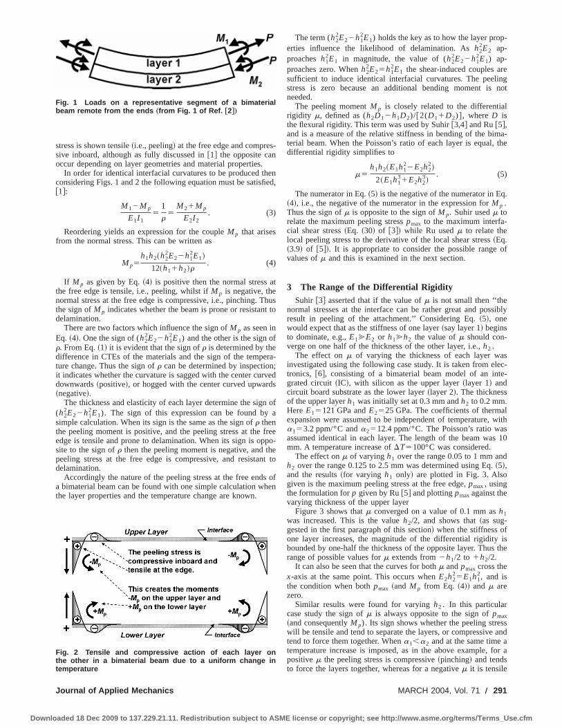
The effect onm of varyingh1 over the range 0.05 to 1 mm anh2 over the range 0.125 to 2.5 mm was determined using Eq.~5!,and the results~for varying h1 only! are plotted in Fig. 3. Alsogiven is the maximum peeling stress at the free edge,pmax, usingthe formulation forp given by Ru@5# and plottingpmax against thevarying thickness of the upper layer

Figure 3 shows thatm converged on a value of 0.1 mm ash1was increased. This is the valueh2/2, and shows that~as sug-gested in the first paragraph of this section! when the stiffness ofone layer increases, the magnitude of the differential rigiditybounded by one-half the thickness of the opposite layer. Thusrange of possible values form extends from2h1/2 to 1h2/2.

It can also be seen that the curves for bothm andpmax cross thex-axis at the same point. This occurs whenE2h2

25E1h12, and is

the condition when bothpmax ~and M p from Eq. ~4!! and m arezero.

Similar results were found for varyingh2 . In this particularcase study the sign ofm is always opposite to the sign ofpmax~and consequentlyM p). Its sign shows whether the peeling strewill be tensile and tend to separate the layers, or compressivetend to force them together. Whena1,a2 and at the same time atemperature increase is imposed, as in the above example,positivem the peeling stress is compressive~pinching! and tendsto force the layers together, whereas for a negativem it is tensile

MARCH 2004, Vol. 71 Õ 291

cense or copyright; see http://www.asme.org/terms/Terms_Use.cfm

s

esmf

m

u

w

tt

b

h

t

ilx

tat

Theeirlin-theat

hows.

of

een

fthen:

-

y

-

is

ey

s

of

4,

Downl

and tends to force them apart.~Thus the differential rigiditym canbe used as an alternative toM p in indicating whether a beam iprone or resistant to delamination.!

In Fig. 3 pmax is always negative except in the unlikely caswhere the upper layer is thinner than 0.091 mm; this implieresistance to delamination. Note, however, that generally thermechanical stress in ICs arises from a temperature reductionthe curing temperature of an epoxy~usually 150°C or 175°C) toroom temperature, or to a test extreme such as265°C. Thus thecase study example is in reality prone to peeling under norusage.

An investigation was also made into the effect onm andpmax ofvarying E1 andE2 . This again showed that the range of possibvalues form was from 2h1/2 to 1h2/2. However, it was alsofound that as the moduli of elasticity increased, the maximpeeling stresspmax increased in proportion.

4 ConclusionsThe sign of the interfacial free-edge peeling momentM p indi-

cates whether a bimaterial beam is prone or resistant to delamtion under thermomechanical stress. This sign can be foundone simple calculation when the layer properties and the tempture change are known. The relationship between the peelingmentM p and the differential rigiditym of the bimaterial beam wasexamined. It was shown that there is a close relationship, andthe sign of the differential rigidity is also a direct indicator of thresistance—or the tendency—to peeling. Finally it was shownupper and lower limits to the value of the differential rigidiexist; as the stiffness of one layer becomes dominant, the matude of the differential rigidity converges to one-half the thickneof the opposite layer.

References@1# Moore, T. D., and Jarvis, J. L., 2003, ‘‘A Simple and Fundamental Design R

for Resisting Delamination in Bimaterial Structures,’’ Microelectron. Relia43~3!, pp. 487–494.

@2# Timoshenko, S., 1925, ‘‘Analysis of Bi-metal Thermostats,’’ J. Opt. Soc. Am11~Sept.!, pp. 233–255.

@3# Suhir, E., 1986, ‘‘Stresses in Bi-metal Thermostats,’’ ASME J. Appl. Mec53, pp. 657–660.

@4# Suhir, E., 1989, ‘‘Interfacial Stresses in Bi-metal Thermostats,’’ASME J. ApMech.,56, pp. 595–600.

@5# Ru, C. Q., 2002, ‘‘Interfacial Thermal Stresses in Bimaterial Beams: ModifiBeam Models Revisited,’’ ASME J. Electron. Packag.,124, pp. 141–146.

@6# Moore, T. D., and Jarvis, J. L., 2001, ‘‘Failure Analysis and Stress Simulain Small Multichip BGAs,’’ IEEE Trans. Adv. Packag.,24~2!, pp. 216–223.

Triple Coordinate Transforms forPrediction of Falling Cylinder Throughthe Water Column

Peter C. Chu, Chenwu Fan, Ashley D. Evans,and Anthony GillesNaval Ocean Analysis and Prediction Laboratory,Department of Oceanography, Naval Postgraduate Sch833 Dyer Road, Monterey, CA 93943

Triple coordinate systems are introduced to predict translatand orientation of falling rigid cylinder through the water coumn: earth-fixed coordinate (E-coordinate), cylinder’s main-afollowing coordinate (M-coordinate), and hydrodynamic force folowing coordinate (F-coordinate). Use of the triple coordinasystems and the transforms among them leads to the simplificof the dynamical system. The body and buoyancy forces and

292 Õ Vol. 71, MARCH 2004 Copyright © 2

oaded 18 Dec 2009 to 137.229.21.11. Redistribution subject to ASME li

sao-

rom

al

le

m

ina-ith

era-mo-

thatehatygni-ss

ule.,

.,

.,

pl.

ed

ion

ool,

on-isl-etionheir

moments are easily calculated using the E-coordinate system.hydrodynamic forces (such as the drag and lift forces) and thmoments are easily computed using the F-coordinate. The cyder’s moments of gyration are simply represented usingM-coordinate. Data collected from a cylinder-drop experimentthe Naval Postgraduate School swimming pool in June 2001 sgreat potential of using the triple coordinate transform@DOI: 10.1115/1.1651093#

1 IntroductionConsider an axially symmetric cylinder with the centers

mass~X! and volume~B! on the main axis~Fig. 1!. Let (L,d,x)represent the cylinder’s length, diameter, and the distance betwthe two points~X,B!. The positivex-values refer to nose-downcase, i.e., the center of mass~COM! is lower than the center ovolume ~COV!. Three coordinate systems are used to modelhydrodynamics of falling cylinder through the water columearth-fixed coordinate~E-coordinate!, cylinder’s main-axis fol-lowing coordinate~M-coordinate!, and hydrodynamic force fol-lowing coordinate ~F-coordinate!. All the systems are threedimensional, orthogonal, and right-handed.

2 Triple Coordinate Systems

2.1 E-Coordinate. The E-coordinate is represented bFE~O,i,j ,k) with the origin ‘‘O,’’ and three axes:x, y-axes~hori-zontal! with the unit vectors~i,j ! and z-axis~vertical! with the unitvectork ~upward positive!. The position of the cylinder is represented by the position of the COM,

X5xi1yj1zk, (1)

which is translation of the cylinder. The translation velocitygiven by

dX

dt5V, V5~u,v,w!. (2)

2.2 M-Coordinate. Let orientation of the cylinder’s main-axis ~pointing downward! is given by iM . The angle betweeniMandk is denoted byc21p/2. Projection of the vectoriM onto the(x,y) plane creates angle (c3) between the projection and thx-axis ~Fig. 2!. The M-coordinate is represented bFM(X,iM ,jM ,kM) with the origin ‘‘X,’’ unit vectors (iM ,jM ,kM),and coordinates (xM ,yM ,zM). In the plane consisting of vectoriM andk ~passing through the pointM, called the IMK plane!, twonew unit vectors (jM ,kM) are defined withjM perpendicular to theIMK plane, andkM perpendicular toiM in the IMK plane. The unitvectors of the M-coordinate system are given by~Fig. 2!

j M5k3 iM , kM5 iM3 j M . (3)

The M-coordinate system is solely determined by orientationthe cylinder’s main-axisiM . Let the vectorP be represented byEPin the E-coordinate and byMP in the M-coordinate, and letM

E R bethe rotation matrix from the M-coordinate to the E-coordinate,

ME R~c2 ,c3![F r 11 r 12 r 13

r 21 r 22 r 23

r 31 r 32 r 33

G5F cosc3 2sinc3 0

sinc3 cosc3 0

0 0 1G

3F cosc2 0 sinc2

0 1 0

2sinc2 0 cosc2

G , (4)

Contributed by the Applied Mechanics Division of THE AMERICAN SOCIETY OFMECHANICAL ENGINEERSfor publication in the ASME JOURNAL OF APPLIED ME-CHANICS. Manuscript received by the ASME Applied Mechanics Division, May 12003; final revision, Sept. 19, 2003. Associate Editor: D. A. Siginer.

004 by ASME Transactions of the ASME

cense or copyright; see http://www.asme.org/terms/Terms_Use.cfm

-

p

y

isee

Downl

which represents (iM ,jM ,kM),

iM5F r 11

r 21

r 31

G , j M5F r 12

r 22

r 32

G , kM5F r 13

r 23

r 33

G . (5)

Transformation ofMP into EP contains rotation and translation,

EP5ME R~c2 ,c3!MP1X. (6)

Fig. 3 Effect on m and p max of varying upper layer thickness

Fig. 1 M-coordinate with the COM as the origin X and „ im,jm…as the two axes. Here, x is the distance between the COV „B…

and COM, „L ,d … are the cylinder’s length and diameter.

Journal of Applied Mechanics

oaded 18 Dec 2009 to 137.229.21.11. Redistribution subject to ASME li

Let the cylinder rotate around (iM ,jM ,kM) with angles(w1 ,w2 ,w3) ~Fig. 2!. The angular velocity of cylinder is calculated by

v15dw1

dt, v25

dw2

dt, v35

dw3

dt, (7)

and

c15w1 ,dc2

dt5

dw2

dt5v2 ,

dc3

dtÞ

dw3

dt. (8)

If ( v1 ,v2 ,v3) are given, time integration of~7! with the timeinterval Dt leads to

Dw15v1Dt, Dw25v2Dt, Dw35v3Dt. (9)

The increments (Dc2 ,Dc3) are determined by the relationshibetween the two rotation matricesM

E R(c21Dc2 ,c31Dc3) and

ME R(c2 ,c3)

ME R~c21Dc2 ,c31Dc3!

5ME R~c2 ,c3!F cos~Dw3! 2sin~Dw3! 0

sin~Dw3! cos~Dw3! 0

0 0 1G

3F cos~Dw2! 0 sin~Dw2!

0 1 0

2sin~Dw2! 0 cos~Dw2!G . (10)

2.3 F-Coordinate. The F-coordinate is represented bFF(X,iF ,jF ,kF) with the origin X, unit vectors (iF ,jF ,kF), andcoordinates (xF ,yF ,zF). Let Vw be the fluid velocity. The water-to-cylinder velocity is represented byVr5Vw2V, that is decom-posed into two parts,

Vr5V11V2 , V15~Vr• iF!iF , V25Vr2~Vr• iF!iF ,(11)

whereV1 is the component paralleling to the cylinder’s main-ax~i.e., along iM), and V2 is the component perpendicular to thcylinder’s main-axial direction. The unit vectors for thF-coordinate are defined by~column vectors!

iF5 iM5F r 11

r 21

r 31

G , jF5V2 /uV2u, kF5 iF3 jF . (12)

Fig. 2 Three coordinate systems

MARCH 2004, Vol. 71 Õ 293

cense or copyright; see http://www.asme.org/terms/Terms_Use.cfm

ev

-

h

dhe

ity

r for

yoy-

he

e

e

ith

Downl

The F-coordinate system is solely determined by orientation ofcylinder’s main-axis (iM) and the water-to-cylinder velocity. Notthat the M and F-coordinate systems have one common unittor iM ~orientation of the cylinder!.

Let FER be the rotation matrix from the F-coordinate to th

E-coordinate,

FER~c2 ,c3 ,fMF![F r 11 r 128 r 138

r 21 r 228 r 238

r 31 r 328 r 338G , fMF[~ j M ,jF!,

(13)

which leads to

iF5F r 11

r 21

r 31

G , jF5F r 128

r 228

r 328G , kF5F r 138

r 238

r 338G . (14)

Here,fMF is the angle between the two unit vectors (j M ,jF). Letthe vectorP be represented byFP in the F-coordinate. Transformation ofFP into EP contains rotation and translation,

EP5FER~c2 ,c3 ,fMF!FP1X. (15)

Use of the F-coordinate system simplifies the calculations forlift and drag forces and torques acting on the cylinder. SinceM and F-coordinates share a common axisiM5 iF , the rotationmatrix from the F to M-coordinate systems is given by

FMR5E

MR EFR5M

E R21~c2 ,c3!FER~c2 ,c3 ,fMF!

5F 1 0 0

0 e22 e23

0 e32 e33

G , (16)

is two-dimensional with the rotation matrix given by

FME5@e2 e3#, e25Fe22

e32G , e35Fe23

e33G . (17)

Let the cylinder rotate around (iF ,jF ,kF) with the angular ve-locity components represented by (v18 ,v28 ,v38) ~Fig. 2!. They areconnected to the angular velocity components in the M-coordinsystem by

v185v1 , Fv28

v38G5M

F EFv2

v3G . (18)

3 Prediction of Hydrodynamic Characteristicsof Falling Cylinder

3.1 Translation Velocity. The translation velocity of thecylinder ~V! is governed by the momentum equation in tE-coordinate system,

Table 1 Physical parameters of the model cylinders

Cylinder Mass~g! L (cm)Volume~cm3!

rm

~g m23!

J1

~g m2!

x~cm!

J2(J3)~g m2!

322.5 15.20 191.01 1.69 330.5 0.00 60871 0.74 5783.0

1.48 6233.82 254.2 12.10 152.05 1.67 271.3 0.06 3424

0.53 3206.51.00 3312.6

3 215.3 9.12 114.61 1.88 235.0 0.00 16950.29 1577.50.58 1556.8

294 Õ Vol. 71, MARCH 2004

oaded 18 Dec 2009 to 137.229.21.11. Redistribution subject to ASME li

the

ec-

e

thethe

ate

e

d

dt F uvwG52F 0

0~12rw / r !g

G11

rP F Fx

Fy

Fz

G , (19)

whereg is the gravitational acceleration;r is the average cylinderdensity;rw is the water density;P is the cylinder volume; andrP5m, is the cylinder mass; (Fx ,Fy ,Fz) are the hydrodynamicforce ~including drag and lift forces! components. The drag anlift forces are calculated using the drag and lift laws with tgiven water-to-cylinder velocity (Vr) that is calculated using theF-coordinate.

3.2 Cylinder’s Orientation. It is convenient to write themoment of momentum equation

J•dv

dt5Mb1Mh , (20)

in the M-coordinate system with the cylinder’s angular veloccomponents (v1 ,v2 ,v3) defined by~7!. Here,Mb andMh are thebody and surface force torques. The moment of gyration tensothe axially symmetric cylinder is a diagonal matrix

J5F J1 0 0

0 J2 0

0 0 J3

G , (21)

where J1 , J2 , and J3 are the moments of inertia. The gravitforce, passing the COM, doesn’t induce the moment. The buancy force induces the moment in thejM direction if the COMdoesn’t coincide with the COV~i.e., xÞ0!,

Mb5Pxrwg cosc2jM . (22)

The moment of the hydrodynamic force iniF direction is notcaused by the drag and lift forces, but by the viscous fluid. Tmoment of the viscous force is calculated by~White @1#!

M v152Cm1v1iF , Cm1[pmLd2. (23)

When the cylinder rotates aroundjF with the angular velocityv28 ,the drag force exerts the torque on the cylinder in thejF direction(Md2) and in thekF direction (Md3). The lift force exerts thetorque on the cylinder in thejF direction (M l2). The moment ofhydrodynamic forceMh

Mh5M v11Md21Md31M l2 (24)

.9

.6

.2

Table 2 Trajectory patterns

TrajectoryPattern

Description

Straight Cylinder exhibited little angular change aboutz-axis. Theattitude remained nearly parallel with z-axis~615 deg!.

Slant Cylinder exhibited little angular change about z-axis. Thattitude was 45 deg offz-axis ~615 deg!.

Spiral Cylinder experienced rotation aboutz-axis throughout thewater column

Flip Initial water entry point rotated at least 180 degFlat Cylinder’s angle with vertical near 90 deg for most of th

trajectorySeesaw Similar to the flat pattern except that cylinder’s angle w

vertical would oscillate between greater~less! than 90 degand less~greater! than 90 deg like a seesaw

Combin-ation

Complex trajectory where cylinder exhibited severalof theabove patterns

Transactions of the ASME

cense or copyright; see http://www.asme.org/terms/Terms_Use.cfm

Downl

Fig. 3 Cylinders’ track patterns observed during CYDEX

is represented in M-coordinate. Note that the M and F-coordinsystems have the samex-axis, iM5 iF . The equations for(v1 ,v2 ,v3) are given by

dv1

dt52a1v1 , (25)

d

dt Fv2

v3G52B•Fv2

v3G1a2 , (26)

where

Journal of Applied Mechanics

oaded 18 Dec 2009 to 137.229.21.11. Redistribution subject to ASME li

atea1[

Cm1

J158pmL/m,

B[F 1

J20

01

J3

G •~Cm2e2e2T1Cm3e3e3

T2Cmle2e3T!,

(27)

MARCH 2004, Vol. 71 Õ 295

cense or copyright; see http://www.asme.org/terms/Terms_Use.cfm

296 Õ Vol. 71,

Downloaded 18 Dec 2009

Table 3 Trajectory patterns for nose-down dropping „xÌ0…

Cylinder Length~cm! 15.20 12.10 9.12x ~cm! 1.48 1.00 0.58

Drop angle 15 deg Straight~1! Straight~1!, Spiral ~1! Spiral* ~2!Slant-straight* ~3! Slant-straight* ~2! Straight-slant~1!

Slant-straight~1!Drop angle 30 deg Straight~1! Slant ~1!, Spiral ~1! Spiral* ~5!

Slant-straight* ~4! Straight~1!Slant-straight* ~2!

Drop angle 45 deg Slant* ~2!, Straight~1! Straight~1! Spiral* ~4!Slant-straight~1! Spiral* ~2! Slant-spiral~1!Straight-spiral~1! Straight-spiral~1!

Slant-straight~1!Drop angle 60 deg Straight** ~5! Straight* ~3! Spiral* ~4!

Straight-spiral~1! Straight-spiral~1!Straight-slant~1!

Drop angle 75 deg Straight** ~5! Straight~2! Spiral ~2!, Slant~1!Straight-spiral~3! Straight-spiral~2!

t

d ofinof

ri-

ionrs’ablede

a2[F 1

J20

01

J3

G •~M1e22M3e3!1Pxgrw

J2cosc2F10G .

Here, Ml[1/2drw /(11 f r)LV22x, M3[1/2Cd2drw /(1

1 f r)V22Lx, and f r is the added mass factor for the moment

drag and lift forces. Equation~25! has the analytical solution

v1~ t !5v1~ t0!exp@2a1~ t2t0!#, (28)

which represents damping rotation of the cylinder aroundmain axis (iM). The Euler-typed forward difference is usedsolve the five Eqs.~19!, ~26!, and~28!.

MARCH 2004

to 137.229.21.11. Redistribution subject to ASME li

of

theo

4 Model Evaluation

The Cylinder Drop Experiment~CYDEX! was conducted at theNaval Postgraduate School~NPS! in July 2001~Chu et al.@2#! toevaluate the three-dimensional theoretical model. It consistedropping cylinders whose physical conditions are illustratedTable 1 into the water and recording the position as a functiontime using two digital cameras at~30 Hz! as the cylinders fell 2.4meters to the pool bottom. After analyzing the CODEX expemental data, seven general trajectory patterns~Table 2! are iden-tified: straight, slant, spiral, flip, flat, see-saw, and combinat~Fig. 3!. Dependence of the trajectory patterns on the cylindephysical parameters and release conditions are illustrated in T3. The theoretical model predicts the motion of cylinder insi

Fig. 4 Movement of Cylinder #1 „LÄ15.20 cm, rÄ1.69 g cm À3… with xÄ0.74 cm

and drop angle 45 deg obtained from „a… experiment, and „b… recursive model

Transactions of the ASME

cense or copyright; see http://www.asme.org/terms/Terms_Use.cfm

Journal of Applied Mec

Downloaded 18 Dec 2009 to 137.

Fig. 5 Movement of Cylinder #2 „LÄ12.10 cm, rÄ1.67 g cm À3… with xÄÀ1.00

cm and drop angle 30 deg obtained from „a… experiment, and „b… recursivemodel

e

a

red

flipee

theer

s in

d

nvert

the water column reasonably well. Two examples are listedillustration.

Positive x „Nose-Down…. Cylinder #1 (L515.20 cm, r51.69 g cm23) with x50.74 m is injected to the water with thdrop angle 45 deg. The physical parameters of this cylindergiven by

m5322.5 g, J15330.5 g cm2, J25J355783.0 g cm2.(29a)

Undersea cameras measure the initial conditions

x050, y050, z050, u050, v0521.55 m s21,

w0522.52 m s21,(29b)

c1050, c20560 deg, c305295 deg, v1050,

v2050.49 s21, v3050.29 s21.

Substitution of the model parameters~29a! and the initial condi-tions~29b! into the theoretical model~~19!, ~26!, ~28!! leads to theprediction of the cylinder’s translation and orientation that acompared with the data collected during CYDEX at time ste~Fig. 4!. Both model simulated and observed tracks show a slstraight pattern.

Negative x „Nose-Up…: Cylinder #2 (L512.10 cm, r51.67 g cm23) with x521.00 cm is injected to the water withthe drop angle 30 deg. The physical parameters of this cylinare given by

m5254.2 g, J15271.3 g cm2, J25J353312.6 g cm2.(30a)

Undersea cameras measure the initial conditions

hanics

229.21.11. Redistribution subject to ASME li

for

are

repsnt-

der

x050, y050, z050, u050, v0520.75 m s21,

w0520.67 m s21,(30b)

c1050, c20524 deg, c305296 deg, v1050,

v20525.08 s21, v3050.15 s21.

The predicted cylinder’s translation and orientation are compawith the data collected during CYDEX at time steps~Fig. 5!. Thesimulated and observed tracks show flip-spiral pattern. Theoccurs at 0.11 s~0.13 s! after cylinder entering the water in thexperiment~model!. After the flip, the cylinder spirals down to thbottom.

5 Conclusions~1! Triple coordinate systems are suggested to predict

translation and orientation of falling rigid cylinder through watcolumn: earth-fixed coordinate~E-coordinate!, cylinder’s main-axis following coordinate~M-coordinate!, and hydrodynamicforce following coordinate~F-coordinate!. It simplifies the com-putation with the body and buoyancy forces and their momentthe E-coordinate system, the hydrodynamic forces~such as thedrag and lift forces! and their moments in the F-coordinate, anthe cylinder’s moments of gyration in the M-coordinate.

~2! Usually, the momentum~moment of momentum! equationfor predicting the cylinder’s translation velocity~orientation! isrepresented in the E-coordinate~M-coordinate! system. Transfor-mations among the three coordinate systems are used to cothe forcing terms into E-coordinate~M-coordinate! for the mo-

MARCH 2004, Vol. 71 Õ 297

cense or copyright; see http://www.asme.org/terms/Terms_Use.cfm

tr

h

i

ba

ca

na

oc

e

s

gets

sin-oellinnd

ion

b-rn-toishey of

o

go-con-

ofhes theain

on-e

dary

thely

twora-to-

Downl

mentum~moment of momentum! equation. A numerical model isdeveloped on the base of the triple coordinate transform to prethe cylinder’s translation and orientation.

~3! Model-experiment comparison shows that the model wpredicts the cylinder’s translation and orientation. However,performance of the numerical model forx50 is not as good as foxÞ0.

AcknowledgmentsThis research was funded by the Office of Naval Resea

Coastal Geosciences Program~grant N0001403WR20178!, theNaval Oceanographic Office, and the Naval Postgraduate Scsupported this study.

References@1# White, F. M., 1974,Viscous Fluid Flow, 1st Ed., McGraw-Hill, New York.@2# Chu, P. C., Gilless, A. F., Fan, C., and Fleischer, P., 2002, ‘‘Hydrodynam

Characteristics of a Falling Cylinder in the Water Column,’’Advances in FluidMechanics, 4, M. Rahman, R. Verhoeven, and C. A. Brebbia, eds., WIT PreSouthampton, UK, pp. 163–181.

Determination of Loads in anInextensible Network According toGeometry of Its Wrinkles

Cheng LuoBiomedical Engineering and Institute forMicromanufacturing, Louisiana Tech University, 911Hergot Avenue, Ruston, LA 71272e-mail: chengluo@latech.edu

This note derives an analytical relationship for an inextensinetwork when it buckles. According to the relationship, theplied compressive force can be determined according to the mmum absolute values of deflection and angle of deflection innetwork’s wrinkles. @DOI: 10.1115/1.1651094#

1 IntroductionIf we pull both ends of a thin plastic sheet used for food pa

aging, a set of wrinkles, parallel to the loading direction, appeCerda and Mahadevan@1# and Cerda et al.@2# showed that thewavelength of the wrinkles is proportional to the square rootthe sample size, and the tension can be determined accordithe wavelength of the wrinkles. Fabric, such as cloth, is usucomposed of two families of inextensible elastic fibers. The Poson effect in the fabric may be different from that in the plassheet. For example, if the two families of fibers are loosely cnected, then the Poisson effect may be neglected, while thisnot be true for the plastic sheet. Therefore, the modeling ofinextensible network may be different from that of a plastic sheIn this note, we demonstrate that the applied compressive forcthe fabric can be determined according to the maximum absovalues of deflection and angle of deflection in its wrinkles.

The effects of bending stiffness of a fiber network or an elasurface have been well studied in the literature. Simmonds@3#considered elastic surfaces with resistance to strain and flex

Contributed by the Applied Mechanics Division of THE AMERICAN SOCIETY OFMECHANICAL ENGINEERSfor publication in the ASME JOURNAL OF APPLIED ME-CHANICS. Manuscript received by the ASME Applied Mechanics Division, June2003, final revision, September 19, 2003. Associate Editor: O. O’Reilly.

298 Õ Vol. 71, MARCH 2004

oaded 18 Dec 2009 to 137.229.21.11. Redistribution subject to ASME li

dict

ellhe

rch

ool

cal

ss,

lep-axi-the

k-rs.

ofg tollyis-

ticn-an-anet.on

lute

tic

ure,

and Wang and Pipkin@4,5# studied inextensible nets with bendinstiffness. Hilgers and Pipkin developed a theory of elastic shein a series of papers,@6–9#, by introducing the second derivativeof the deformation as well as the first derivatives into the straenergy density. Hilgers@10# also examined dynamic effects. Luand Steigmann@11# established a model, a generalized plate/shtheory, to take into account the effects of bending and twistingthe inextensible networks for finite deformations in 3-space, averified the soundness of a special form of finite-deformatplate theory developed by Wang and Pipkin in@4#. Wang andPipkin @4# used their theory to consider the Euler buckling prolem of a flat inextensible network, and indicated that the goveing equation of the flat sheet during the buckling is identicalthat for finite-amplitude oscillation of a simple pendulum. In thwork, we further explore the buckling problem to determine tapplied load on the inextensible network according to geometrits wrinkles.

2 An Analytical RelationshipConsider a flat sheet that initially occupies the region 0,x

,L, 0,y,H in the x-y plane. The sheet is composed of twfamilies of inextensible fibers, which initially lie parallel to thexand y-axes; thus every linex5constant ory5constant in the re-gion is regarded as a fiber. The two families of fibers are orthonal in the reference configuration. They are assumed to betinuously distributed and fastened together at their pointsintersection to prevent slipping of one fiber family relative to tother. The sheet is treated as a continuum. Each fiber meetBernoulli-Euler hypotheses: cross sections of each fiber remplane, suffer no strain, and are normal to the fiber in every cfiguration. A uniform forceT per unit length is applied to the edgx5L as a dead load along the negative direction ofx-axis ~seeFig. 1!, and edgesy50 andy5H are free from applied tractionsand couples and displacement restrictions. The possible bounconditions of physical meaning on the sidesx50 andx5L can beclassified into four categories:~i! both sidesx50 andx5L aresimply supported;~ii ! the sidex50 is clamped and the sidex5L is free; ~iii ! both sidesx50 andx5L are clamped; and~iv!the sidex50 is clamped and the sidex5L is simply supported.For any set of those boundary conditions, a solution is thatfamily of fibers withx5constant remain straight lines, the famiof fibers with y5constant have identical deflections in thex-zplane and have no deflections in the other planes, and thefamilies of fibers are still orthogonal in the deformed configution ~see Fig. 2!. Let u(x) denote the angle between the tangentthe deflection curve and thex-y plane. Then it satisfies the equation, @4#,

2,

Fig. 1 Top view of the flat sheet before wrinkling

Fig. 2 Side view of a possible deformed configuration of thesheet

Transactions of the ASME

cense or copyright; see http://www.asme.org/terms/Terms_Use.cfm

h

i

f

o

n

f

g

at

i

m

s.onskled

in

theloth

bei-

ctse.,s

tis-

toftertion

ndnt-

g,’’

in-

s,’’

g

th

Downl

d2u~x!

dx21 f sinu~x!50, (1)

wheref 5T/G andG represents the bending stiffness of the sheThe boundary conditions in each category can be expresseterms ofu(x) as follows:

~ i! u~0!5u0 ,du~x!

dx Ux50

50,du~x!

dx Ux5L

50; (2)

~ ii ! u~0!5u0 ,du~x!

dx Ux5L

50; (3)

~ iii ! u~0!5u0 , u~L !5u0 or 2u0 ; (4)

~ iv! u~0!5u0 ,du~x!

dx Ux5L

50. (5)

Let w(x) denote the deflection of the family of fibers wity5constant. Then, using Eq.~14.5! of @4# and noting that thebending couple is2Tw(x), we have

w~x!52G

T

du~x!

dx. (6)

The condition~6! describes the relationship of the deflection wthe forceT and the change in the angle of deflection. We desiremake this relationship more explicit for easy determination oTaccording to the geometry of the wrinkles. From~6!, it can beseen that

w05G

T Udu~x!

dx Umax

, (7)

where w0 denotes the maximum absolute value of deflectiNext, we determineudu(x)/dxumax first in Case~i! and then in theother three cases.

Rewrite ~1! as

1

2

d

du~x! S du~x!

dx D 2

1 f sinu~x!50. (8)

With the help of~2!1 and ~2!2 , we obtain

S du~x!

dx D 2

52 f ~cosu~x!2cosu~L !!, (9)

which is the first integral of~8!. There are two approaches tobtain the maximum value of (du(x)/dx)2 and consequentlyudu(x)/dxumax: 1. first solve~9! to find the analytical expressioof u(x), and then substitute it back into~9! to obtain the maxi-mum value of (du(x)/dx)2, and 2. consider the similarity between this buckling problem and the oscillation behavior osimple pendulum. As indicated in Wang and Pipkin@4#, with xinterpreted as time, the ordinary differential equation~1! is thegoverning equation for finite-amplitude oscillation of a simppendulum,@12#, and Eq.~9! corresponds to conservation of enerin the pendulum equations. If we use the first approach, therived mathematical expression ofu(x) will involve elliptic func-tions, which increase efforts to find the maximum value(du(x)/dx)2, while the second approach has a straightforwphysical meaning and is easily visualized. Therefore, we adopsecond approach here. The conditions~2! state that the pendulumis at its maximum deflectionu0 at time 0 with the speed 0 and hathe speed 0 at timeL. This indicates thatu0 is its amplitude ofoscillation~without loss of generality,u0 is assumed to be a postive value, and the derived result~11! is also true ifu0 is supposedto be negative!, L is an even multiple of one-quarter of the perioof the pendulum,u(L)5u0 or 2u0 , and 2u0<u(x)<u0 ~seeFig. 3 for an illustration!. Consequently, it can be observed fro~9! that (du(x)/dx)2 has the maximum value atu(x)50, i.e.,

Journal of Applied Mechanics

oaded 18 Dec 2009 to 137.229.21.11. Redistribution subject to ASME li

et.d in

thto

n.

o

-a

leyde-

ofrdthe

s

-

d

S du~x!

dx Dmax

2

52 f ~12cosu~L !!. (10)

By ~7! and ~10!, we find the relationship ofT with w0 andu0

T52G~12cosu0!

w02

. (11)

Using the same procedures as the above for Case~i!, we canfind that the relationship~11! also holds in the other three caseTherefore, we conclude that, no matter what boundary conditia buckled sheet has, the compressive force applied on the bucsheet can be determined using the relationship~11! after we mea-sure the maximum values of deflection and angle of deflectionthe wrinkles. The independence of~11! on the boundary condi-tions implies that the relationship can be used to determineapplied load not only in the rectangular sheet, but also in the cor curtain whose local area is wrinkled.

3 DiscussionsFor ~11! to hold, the Poisson effect in the network needs to

negligibly small, which is true, for example, when the two famlies of fibers are loosely connected. Since the relationship~11!was obtained using the solution for a simple pendulum, it subjeto the physical limitation for the simple pendulum as well, i.2p/2,u(x),p/2. This implies that if the angle of deflection ibeyond that range, the relationship~11! is not applicable. In addi-tion, it can be observed that the governing equation~1! and theanalytical expressions of the boundary conditions~2!–~5! areidentical to those for a buckled inextensible rod which also safies the Bernoulli-Euler hypotheses,@13#. Therefore, the relation-ship~11! holds for the inextensible rod as well, and can be useddetermine the compressive force in its buckled configuration aits maximum absolute values of deflection and angle of deflecare measured.

AcknowledgmentThe author would like to thank two anonymous reviewers a

Prof. Oliver O’Reilly in the Mechanical Engineering Departmeat the University of California at Berkeley for their helpful comments on the paper.

References@1# Cerda, E., and Mahadevan, L., 2003, ‘‘Geometry and Physics of Wrinklin

Phys. Rev. Lett.,90, 074302.@2# Cerda, E., Ravi-Chandar, K., and Mahadevan, L., 2002, ‘‘Thin Films: Wr

kling of an Elastic Sheet Under Tension,’’ Nature~London!, 419, pp. 579–580.@3# Simmonds, J. G., 1985, ‘‘The Strain Energy Density of Rubber-Like Shell

Int. J. Solids Struct.,21, pp. 67–77.@4# Wang, W.-B., and Pipkin, A. C., 1986, ‘‘Inextensible Networks With Bendin

Stiffness,’’ Q. J. Mech. Appl. Math.,39, pp. 343–359.@5# Wang, W.-B., and Pipkin, A. C., 1986, ‘‘Plane Deformations of Nets Wi

Bending Stiffness,’’ Acta Mech.,65, pp. 263–279.

Fig. 3 „a… Side view of a possible deformed configuration ofthe sheet in Case „i…, and „b… its equivalent state in a simplependulum

MARCH 2004, Vol. 71 Õ 299

cense or copyright; see http://www.asme.org/terms/Terms_Use.cfm

f

i

i

t

the

Downl

@6# Hilgers, M. G., and Pipkin, A. C., 1992, ‘‘Elastic Sheets With Bending Stiness,’’ Q. J. Mech. Appl. Math.,45, pp. 57–75.

@7# Hilgers, M. G., and Pipkin, A. C., 1992, ‘‘Bending Energy of Highly ElastMembranes,’’ Q. Appl. Math.,50, pp. 389–400.

@8# Hilgers, M. G., and Pipkin, A. C., 1993, ‘‘Energy Minimizing Deformations oElastic Sheets With Bending Stiffness,’’ J. Elast.,31, pp. 125–139.

@9# Hilgers, M. G., and Pipkin, A. C., 1996, ‘‘Bending Energy of Highly ElastMembranes II,’’ Q. Appl. Math.,54, pp. 307–316.

@10# Hilgers, M. G., and Pipkin, A. C., 1997, ‘‘Plane Infinitesimal Waves in Elas

300 Õ Vol. 71, MARCH 2004

oaded 18 Dec 2009 to 137.229.21.11. Redistribution subject to ASME li

f-

c

f

c

ic

Sheets With Bending Stiffness,’’ Math. Mech. Solids,2, pp. 75–89.@11# Luo, C., and Steigmann, D. J., 2001, ‘‘Bending and Twisting Effects in

Three-Dimensional Finite Deformations of an Inextensible Network,’’Ad-vances in the Mechanics of Plates and Shells, Kluwer Academic Publishers,Boston, pp. 213–228.

@12# Synge, J. L., and Griffith, B. A., 1949,Principles of Mechanics, Second Ed.,McGraw-Hill, New York, pp. 370–372.

@13# Timoshenko, S., 1936,Theory of Elastic Stability, First Ed., McGraw-Hill,New York, pp. 69–75.

Transactions of the ASME

cense or copyright; see http://www.asme.org/terms/Terms_Use.cfm