On Scatterometer Ocean Stress

Proof Only

Proof OnlyOn Scatterometer Ocean Stress

M. PORTABELLA* AND A. STOFFELEN

Royal Netherlands Meteorological Institute (KNMI), De Bilt, The Netherlands

(Manuscript received 8 June 2007, in final form 2 June 2008)

ABSTRACT

Scatterometers estimate the relative atmosphere–ocean motion at spatially high resolution and provide

accurate inertial-scale ocean wind forcing information, which is crucial for many ocean, atmosphere, and

climate applications. An empirical scatterometer ocean stress (SOS) product is estimated and validated using

available statistical information. A triple collocation dataset of scatterometer, and moored buoy and nu-

merical weather prediction (NWP) observations together with two commonly used surface layer (SL) models

are used to characterize the SOS. First, a comparison between the two SL models is performed. Although

their roughness length and the stability parameterizations differ somewhat, the two models show little dif-

ferences in terms of stress estimation. Second, a triple collocation exercise is conducted to assess the true and

error variances explained by the observations and the SL models. The results show that the uncertainty in the

NWP dataset is generally larger than in the buoy and scatterometer wind/stress datasets, but it depends on

the spatial scales of interest. The triple collocation analysis also shows that scatterometer winds are as close to

real winds as to equivalent neutral winds, provided that we use the appropriate scaling. An explanation for

this duality is that the small stability effects found in the analysis are masked by the uncertainty in SL models

and their inputs. The triple collocation analysis shows that scatterometer winds can be straightforwardly and

reliably transformed to wind stress. This opens the door for the development of wind stress swath (level 2)

and gridded (level 3) products for the Advanced Scatterometer (ASCAT) on board Meterological Operation

(MetOp) and for further geophysical development.

1. Introduction

Wind forces motion in the ocean and in turn the

motion in the ocean determines the weather and climate

in large portions of the world. Wind forcing is essential

in El Nino–Southern Oscillation (ENSO) and other

ocean–atmosphere interaction phenomena occurring in

the tropics. As such, a homogeneous wind dataset of

high quality would much advance research on the pre-

diction and mechanisms of seasonal forecasting. Vialard

(2000) emphasizes that wind stress is certainly the most

important forcing in the tropics. Moreover, ocean cir-

culation and ENSO play a key role in the earth’s cli-

mate. Besides tropical needs, there are other obvious

applications of such wind stress product included in the

modeling of the Antarctic circumpolar current, forcing

of the southern oceans, research on the variability and

occurrence of storms, and forcing in complex basins, for

example, the Mediterranean. A continuous wind stress

time series of high temporal and spatial resolution

would aid in the understanding of the unexplained year-

to-year variability of these wind events.

Wind information is available from conventional plat-

form observations, such as ship or buoy. These systems

measure the atmospheric flow at a measurement height

that can vary between 4 and 60 m and, therefore, are not a

direct measure of surface 10-m wind or of stress. Stress

computation requires the transformation of these winds

by planetary boundary layer (PBL) parameterization

schemes to represent the sea surface conditions. These

PBL schemes and, in particular, the surface layer (SL)

schemes embedded in the PBL schemes, have improved

accuracy over the years, (Smith et al. 1992; Donelan et al.

1993; Taylor and Yelland 2001; Bourassa 2006) although

they still contain transformation errors (Brown et al. 2005).

jtechO578

Corresponding author address: Dr. Marcos Portabella, Medi-

terranean Centre for Marine and Environmental Research

(CMIMA), Pg. Marıtim Barceloneta 37-49, Barcelona 08003,

SpainAU1 .

E-mail: [email protected]

* Current affiliation: Unidad de Tecnologıa Marina, CMIM-

CSIC, Barcelona, Spain.

JOBNAME: JTECH 25#10 2008 PAGE: 1 SESS: 8 OUTPUT: Thu Nov 27 00:47:10 2008 Total No. of Pages: 15/ams/jtech/170108/jtechO578

MONTH 2008 P O R T A B E L L A A N D S T O F F E L E N 1

DOI: 10.1175/2008JTECHO578.1

� 2008 American Meteorological Society

Proof Only

Proof OnlyFurthermore, buoy wind observations and, by impli-

cation, the NWP analyses that exploit these data use a

fixed frame of reference. However, the wind stress de-

pends on the difference of motion between atmosphere

and ocean. Kelly et al. (2001) show that the ocean cur-

rents do produce a significant annual bias in the buoy-

derived wind stress estimations. In contrast, they show

that scatterometer observations provide a measure of

the relative motion between atmosphere and ocean and,

therefore, can potentially provide accurate wind stress

information.

Several authors have pointed to the mesoscale

wavenumber gap in NWP wind datasets (e.g., Chelton

et al. 2004; Chelton and Schlax 1996; Stoffelen 1996).

This gap is caused by the sparse conventional observa-

tions at the sea surface but also aloft since NWP data

assimilation systems are four-dimensional (4D) in na-

ture and thus require 4D observations to achieve uni-

form quality. In fact, mesoscale atmospheric waves are

poorly observed. Scatterometers, however, do have the

capability to observe the surface component of the wind

variability on much finer space and time scales. More-

over, scatterometers provide information on the inertial

scale of ocean models and thus can potentially provide

essential information to drive ocean models (e.g., Milliff

2005; Chelton et al. 2004; Chelton and Schlax 1996;

Stoffelen 2008).

Scatterometer wind and stress retrieval

A scatterometer measures the electromagnetic radi-

ation scattered back from ocean gravity–capillary

waves, and it is difficult to validate quantitatively the

relationship between the roughness elements associated

with gravity–capillary waves and the measurements. As

such, empirical techniques are employed to relate mi-

crowave ocean backscatter with geophysical variables.

Since the launch of the European Remote Sensing

Satellites (ERS)—ERS-1 (17 July 1991) and ERS-2

(21 April 1995)—on board the active microwave in-

strument (Attema 1991) operating at 5.4 GHz (C band),

numerous retrieval optimizations and validation studies

have been carried out. Usually the retrieved products

from satellite scatterometers are validated by colloca-

tion with NWP model [e.g., European Centre for Me-

dium Range Forecasts (ECMWF)] background winds,

and/or buoy measurements (Stoffelen 1998a). A multi-

tude of wind observations is available at a reference

height of 10 m, and scatterometer winds are tradition-

ally related to 10-m winds. For ERS scatterometers, the

so-called CMOD5 (Hersbach et al. 2007) geophysical

model function (GMF), which relates the 10-m wind to

the backscatter measurements, is used nowadays by the

European Space Agency (ESA) and the Royal Neth-

erlands Meteorological Institute (KNMI) for wind re-

trieval. Stoffelen (1998a) shows that for varying ocean

wind conditions, the backscatter measurements vary

along a well-defined conical surface in the 3D mea-

surement space; that is, the measurements depend on

two geophysical variables or a 2D vector. CMOD5, in-

deed, well explains the coherent distribution of back-

scatter measurements in measurement space.

Chelton et al. (2001) and Stoffelen (2002) show a high

correlation between scatterometer-retrieved winds and

kinematic wind stress. In fact, scatterometers respond to

sea surface roughness (rather than 10-m wind), which is

closely associated with the wind stress. So, if we collo-

cate wind stress or its equivalent value at 10-m height

(hereafter referred as 10-m neutral wind) to CMOD5

winds and estimate their relationship, we would obtain a

CMOD5 stress model (or CMOD5 neutral wind model)

that potentially explains more of the backscatter vari-

ance than the CMOD5 wind model, since the disturbing

effects of atmospheric stratification in the lowest 10 m

have been eliminated. The GMF would provide the

same conical fits in 3D measurement space, since only

an argument of the CMOD function has been trans-

formed. For example, Milliff and Morzel (2001) use a

10-m neutral wind GMF to transform SeaWinds scat-

terometer winds to stress.

The aim of this paper is to define and validate a

scatterometer transformation from wind speed1 to wind

stress. For such purpose, triple collocations of ERS-2

scatterometer observations, moored buoy observations,

and ECMWF model output are performed. Since the

tropics and the extratropics have very different char-

acteristics in terms of, for example, wind variability,

atmospheric stability, or sea state, two different triple

collocation datasets, one for each region, are used in this

paper (see section 2).

Given the inaccuracy of the SL models (Smith et al.

1992; Taylor and Yelland 2001; Bonekamp et al. 2002),

prior to transforming scatterometer wind to stress, we

first take a close look at them to compare their perfor-

mances. For such purpose, two of the most commonly

used models—that is, the Liu, Katsaros, and Businger

(LKB) model (Liu et al. 1979) and the ECMWF SL

model (Beljaars 1997)—are compared in section 3,

where atmospheric stability and wave age effects are

analyzed in detail for a fixed geophysical dataset. The

intercomparison reveals some small and interesting

differences in the SL models.

1 Note that the transformation only refers to wind and stress

intensities, since the direction of the airflow is assumed to be

constant in the SL.

2 J O U R N A L O F A T M O S P H E R I C A N D O C E A N I C T E C H N O L O G Y VOLUME 25


Proof Only

Proof Only

Stoffelen (1998b) shows that given a triple collocation

dataset, the uncertainty of the three observing systems

can be uniquely determined, provided that one of the

systems is used as reference for calibration (scaling) of

the other two systems. In section 4, we perform the

triple collocation exercise as described by Stoffelen

(1998b) to assess the random error and scaling proper-

ties of both buoy and NWP wind stress derived from the

SL models and to evaluate the common true variance

and system error variances for winds at different

heights. As such, the triple collocation exercise is used

to characterize the scatterometer’s ability to measure

kinematic wind stress, rather than wind, and to recom-

mend a wind-to-stress transformation for the ERS

scatterometer. Finally, a summary of the work and

recommendations for future developments are pre-

sented in section 5.

2. Data

Two triple collocation datasets for the years 2000

(tropical data) and 1999/2000 (extratropical data) are

generated to carry out the work described in this paper.

The three data sources used in these datasets are the

ERS-2 scatterometer, the moored buoy network, and

the ECMWF model.

KNMI produces the scatterometer wind and stress

products within the Ocean and Sea Ice (OSI) and Cli-

mate Monitoring (CM) Satellite Application Facilities

(SAFs) of the European Organization for the Exploi-

tation of Meteorological Satellites (EUMETSAT) and

develops scatterometer wind processing software in the

NWP SAF. In the framework of these SAFs, KNMI has

developed an ERS scatterometer data processing

(ESDP) package for the generation of operational wind

products. As such, ERS-2 ESDP (version 1.0g) 10-m

winds are used in this study.

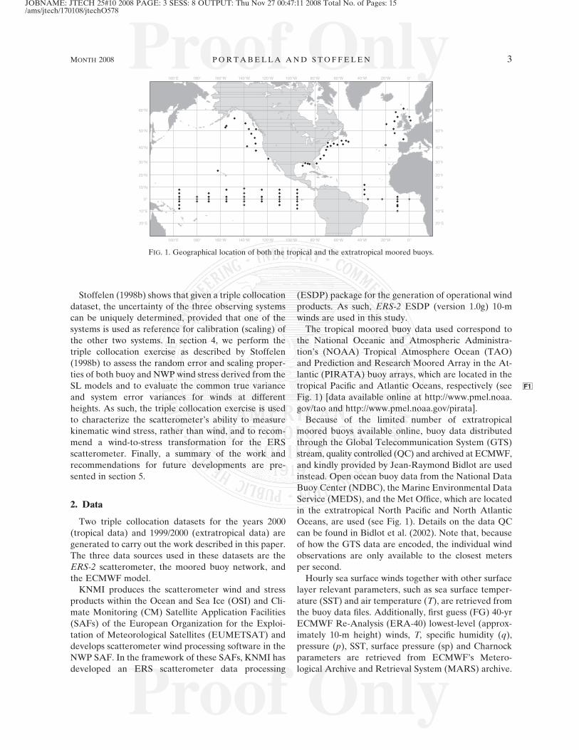
The tropical moored buoy data used correspond to

the National Oceanic and Atmospheric Administra-

tion’s (NOAA) Tropical Atmosphere Ocean (TAO)

and Prediction and Research Moored Array in the At-

lantic (PIRATA) buoy arrays, which are located in the

tropical Pacific and Atlantic Oceans, respectively (see F1

Fig. 1) [data available online at http://www.pmel.noaa.

gov/tao and http://www.pmel.noaa.gov/pirata].

Because of the limited number of extratropical

moored buoys available online, buoy data distributed

through the Global Telecommunication System (GTS)

stream, quality controlled (QC) and archived at ECMWF,

and kindly provided by Jean-Raymond Bidlot are used

instead. Open ocean buoy data from the National Data

Buoy Center (NDBC), the Marine Environmental Data

Service (MEDS), and the Met Office, which are located

in the extratropical North Pacific and North Atlantic

Oceans, are used (see Fig. 1). Details on the data QC

can be found in Bidlot et al. (2002). Note that, because

of how the GTS data are encoded, the individual wind

observations are only available to the closest meters

per second.

Hourly sea surface winds together with other surface

layer relevant parameters, such as sea surface temper-

ature (SST) and air temperature (T), are retrieved from

the buoy data files. Additionally, first guess (FG) 40-yr

ECMWF Re-Analysis (ERA-40) lowest-level (approx-

imately 10-m height) winds, T, specific humidity (q),

pressure (p), SST, surface pressure (sp) and Charnock

parameters are retrieved from ECMWF’s Metero-

logical Archive and Retrieval System (MARS) archive.

FIG. 1. Geographical location of both the tropical and the extratropical moored buoys.



Proof Only

Proof OnlyFG winds do not contain the observed information in

the scatterometer and buoys used in the triple colloca-

tion, such that the FG error and the observed wind er-

rors may be assumed independent.

The triple collocations are performed in the following

way. The ESDP collocation software is used to spatially

and temporally interpolate (linear in space and cubic in

time) the 3-hourly and 1.18 ECMWF ERA-40 forecast

data to the ERS-2 scatterometer data acquisition loca-

tion and time, respectively. In our experience, interpo-

lation errors are negligible using this scheme. Then the

ECMWF–ERS dataset is collocated to the moored buoy

dataset using the following criteria: only observations

separated less than 25 km in distance and 30 min in time

are included in the ECMWF–ERS–BUOY triple col-

location dataset. This implies only one ECMWF–ERS

observation (the closest) per buoy observation. In prac-

tice, most of the collocations are within 12.5 km and

10 min, thus considerably reducing the collocation er-

ror, that is, uncertainty due to spatial and temporal

separation between collocated observations.

Several QC procedures have been applied to this

dataset. The nominal ESDP QC procedure (Stoffelen

1998a) is applied to the ERS-2 retrieved wind dataset,

and only the buoy data with the ‘‘highest quality’’ flag

are used. Moreover, a 4s test is performed to the triple

collocated dataset as in Stoffelen (1998b). The tests are

carefully designed to maintain the main shape of the

wind probability density functions (PDFs).

To avoid uncertainties from unnecessary SL model

height transformations, it seems appropriate to use

wind datasets from a fixed height. In this respect, the

ECMWF ERA-40 winds used here correspond to the

lowest model level, that is, about 10-m height. Since

the extratropical buoy dataset contains many different

buoy systems with different observation heights, a com-

promise between the number of buoys and the observa-

tion height spread is needed. In this paper, only buoy

stations with anemometer heights between 4 and 5 m are

considered (note that all tropical buoys have a fixed

anemometer height of 4 m). In total, we use data from

53 tropical buoy stations and 41 extratropical buoy

stations, which produced 3471 and 3345 collocations

(after quality control), respectively, over the mentioned

periods.

3. Surface layer model comparison

Most of the equations that describe the physical bal-

ances and the turbulent budgets in the lowest 10% of

the PBL—that is, the surface layer—cannot be readily

solved, either because of the presence of highly non-

linear terms or the requirement for enormous in situ

databases (Geernaert 1999). We can alternatively char-

acterize the flow’s dominant dynamic, geometric, and

temporal scales, which involve characteristic time, space,

or velocity scales, by dimensionless groups of variables.

The similarity theory, first postulated by Monin and

Obukov (1954), states that there exists such groups of

variables that have functional relationships to the flow

field and/or fluxes and that these in turn can be used to

characterize the behavior of the higher-order terms of

the above-mentioned equations.

The surface layer is assumed to be a constant flux

layer, and it extends up to a few tens of meters above the

surface. In the bulk parameterization of the similarity

theory, the fluxes are determined with the transfer co-

efficients, which relate the fluxes to the variables mea-

sured, for example, surface wind speed (U), T, SST, and

q. The bulk transfer coefficients can be determined by

integrating the U, T, and q profiles. Close to the surface,

the distributions of U, T, and q are governed by diabatic

processes. As such, the wind profile can be written as

(e.g., Businger 1973)

u�5k

lnz

z0

� �� cðz=LÞ

� � ðU �UsÞ; ð1Þ

where k is the von Karman constant, u* is the friction

velocity, z is the height above the surface, z0 is the

roughness length for momentum, c is the stability

function for momentum (positive, negative, and null for

unstable, stable, and neutral conditions, respectively)

and L is the Monin–Obukhov length, which includes the

effects of temperature and moisture fluctuations on

buoyancy. The wind at the surface Us is neglected

(current effects are statistically investigated in section

4d). Similar profiles to the one in Eq. (1) are also de-

rived for the scale temperature (T*) and the scale hu-

midity (q*) (see Liu et al. 1979). Since stability (z/L)

depends on T and q, the set of three dimensionless

profiles (u*, T*, and q*) has to be solved at the same

time.

Although this paper seeks for the transformation of

wind to kinematic wind stress (u2�) for scatterometers, to

provide a scatterometer wind stress (t) end product

[scatterometer ocean stress (SOS)], knowledge of the

air density (r) is required; that is, t 5 ru2�. Air density

variations can be large. However, r error, which depends

on surface pressure, air temperature, and humidity, is

generally small (1%–2%) and can exceptionally increase

locally in cases such as cold air outflow.

To solve for u*, the wind at certain height—among

other parameters—is required, and z0 and L must be

estimated [see Eq. (1)]. Once u* is estimated, the SL



Proof Only

Proof Onlymodels can be used to compute the wind or its equiva-

lent neutral value at any height (within the SL) just by

modifying z or both z and L in Eq. (1). In other words,

given a wind observation at a certain height (within the

SL), we can estimate the wind and/or the neutral wind at

any height, provided that we first estimate kinematic

stress.

The discussion of air–sea transfer is not about the

validity of the approach described above but generally

about the details of parameter and function choices. As

such, most SL models are based on the bulk formulation

derivation [e.g., Eq. (1)], and differences among them

lie in the parameterization of L and/or z0. This is the

case for the two SL models used in this work, that is,

the LKB and ECMWF SL models. Their similarities

and differences are further discussed in the following

section.

a. LKB versus ECMWF: Formulation

The LKB and ECMWF SL models present the same

roughness length function (see Liu and Tang 1996 and

Beljaars 1997), which is written as

z0 50:11n

u�1

au2�

g; ð2Þ

where n is the kinematic viscosity of the air (1.5 3 1025

m2 s21), g is the gravitational constant of the earth

(9.8 m s22), and a is the (dimensionless) Charnock pa-

rameter (see Charnock 1955). However, the Charnock

value, which is a sea state parameter, is substantially

different—that is, 0.011 for LKB and around 0.018 for

ECMWF SL (the latter is not a fixed value).

The same happens with the formulation of the sta-

bility function c(z/L), which is identical for both

models, but it is where the computation of the L pa-

rameter (Monin–Obukhov length) differs from one

another (see Liu et al. 1979 and Beljaars 1997).

The stand-alone ECMWF SL model uses as input

U, T, q, p, z, SST, surface pressure (sp), and Charnock

data. Similar input is used in LKB; however, the main

difference is that no Charnock input but a default value

of 0.011 is used instead. If q information is not available,

LKB also allows relative humidity (rh) observations as

input. Both SL models can solve for wind stress pro-

vided that U, T, and SST are available—that is, when

humidity and pressure observations are not available,

default values are used instead. Those values are slightly

different, that is, rh 5 0.8 and sp 5 1013 hPa for LKB

versus rh 5 1 and sp 5 1000 hPa for ECMWF.

Additional differences between the two models are

reported in detail in Stoffelen et al. (2006) and Portabella

and Stoffelen (2007) but are found to be minor.

b. LKB versus ECMWF: Results

In this section, we present the most relevant results of

comparing the LKB model against the ECMWF SL

model, using the tropical and extratropical datasets

described in section 2. A more detailed comparison of

the two SL models can be found in Stoffelen et al.

(2006) and Portabella and Stoffelen (2007).

Figure 2 shows F2the two-dimensional histogram of

LKB estimated u* versus ECMWF SL estimated u* for

two different extratropical input datasets: GTS buoys

(Fig. 2a) and ECMWF model output (Fig. 2b). Since the

two datasets contain different parameters (refer to dis-

cussion in section 2) and the two SL models allow

somewhat different input (see section 3a), we use the

coincident parameters (U, T, and SST) for all four

combinations. The results have been, therefore, pro-

duced with fixed Charnock values (default values) for

both models, that is, 0.011 for LKB and 0.018 for

ECMWF. As it is clearly discernible, the distribution

lies close to the diagonal—it is very narrow—and the

correlation is 1, meaning that the estimated u* is very

similar, regardless of the SL model or the dataset used.

Very similar results are found when using the tropical

datasets as input (not shown). In other words, the two

models show very similar stresses.

A 5% bias at high u* values needs to be explained,

though. As described above, SL model differences must

lie in the roughness length and the stability parameters.

Therefore, we take a closer look at these differences.

1) ROUGHNESS TERM

Figure 3 shows the F3same as Fig. 2b but for the z0

parameter. Again, the correlation between the two

models is striking. However, a clear difference between

the two model formulations is noted. As discussed in

section 3a, the Charnock parameter is substantially

different for both models, that is, 0.011 for LKB and

0.018 (default value) for ECMWF. Therefore, for very

low u* values—where the viscosity term [first right-hand

term of Eq. (2)] is dominant—the distribution lies on

the diagonal (same z0 for both models) and for higher

u*—where the Charnock term is dominant [second

right-hand term of Eq. (2)]—the distribution is off di-

agonal, with a slope that is given by the ratio between

the Charnock values of both models.

Looking at Figs. 2b and 3, we can easily realize that to

achieve such good agreement in u* (Fig. 2), the stability

term in Eq. (2) has to compensate for the difference in

the roughness term between the two models. Given that

the roughness term is logarithmic, the difference between

LKB roughness term and ECMWF roughness term is

just a constant, that is, ln�z�zECMWF

0

�5 ln

�z�zLKB

0

��c AU2,



Proof Only

Proof Only

where c 5 ln�aECMWF�

aLKB�ffi 0:5 (using the already-

mentioned LKB and ECMWF default Charnock

values). Since the roughness term ln�z�zLKB

0

�values

vary between 13 (low z0) and 9 (high z0), provided that

the stability term is relatively small in both models,

there should be a scaling of about 5% between ECMWF

and LKB u*, which is not present at low u* values (see

Fig. 2).

2) STABILITY TERM

The relative weight of the stability term in the de-

nominator of Eq. (1) is analyzed for both the LKB and

the ECMWF SL models. It turns out that the stability

term is only relevant for low z0 values (i.e., low winds;

not shown). This is consistent with the bias observed in

Fig. 2, that is, the constant c becomes relevant at in-

creasing z0, since the stability influence becomes mar-

ginal and ln z�zLKB

0

decreases. Moreover, the LKB

stability term is more relevant than the ECMWF sta-

bility term. Since most of the observations correspond

to unstable (c . 0) situations (seeF4 Fig. 4), the more

relevant stability term for LKB compensates the larger

z0 values from the ECMWF SL model, such that the

resulting u* values are very similar for both models.

Given that both SL models use the same stability

functions, we can easily prove that LKB estimates larger

instability (higher negative z/L values) than ECMWF.

Figure 4 shows the histogram of the stability parameter

for both the LKB model (solid line) and the ECMWF SL

model (dotted line), using the extratropical ECMWF

dataset as input. We note larger accumulations at large

negative z/L values for LKB than for ECMWF SL,

indicating larger estimated instability in the former

model. Also note that the stability term is small for

stable cases, since these are close to neutral stability

(i.e., no cases with large, positive z/L). Similar results

are found in the tropics (not shown).

3) SEA STATE EFFECTS

The Charnock parameter is a measure of wave

growth, hence wave age. As mentioned in section 3a, the

Charnock parameter is fixed for LKB but not for the

ECMWF SL model. The Charnock parameter, as for-

mulated in the ECMWF wave model (WAM; docu-

mentation available online at http://www.ecmwf.int/

research/ifsdocs/CY28r1/Waves/), is a function of the

so-called wave-induced stress, which in turn is a func-

tion of the wind input source term (Janssen 2004). Such

Charnock output is included in the collocated ECMWF

dataset (see section 2) and, therefore, can be used as

input to the ECMWF SL model.

Up to now, results have been produced with fixed

Charnock values (default values) for both models, that

is, 0.011 for LKB and 0.018 for ECMWF. To show

the impact of a variable Charnock (i.e., sea state de-

pendency) on the estimated u* uncertainty, we focus

the analysis in the region where the sea state is most

FIG. 2. Two-dimensional histogram of LKB estimated u* vs ECMWF SL estimated u* for two different

extratropical input datasets: (a) GTS buoys and (b) ECMWF model output. The number of data is

denoted by N; mx and my are the mean values along the x and y axes, respectively; m(y 2 x) and s(y 2 x)

are the bias and the standard deviation with respect to the diagonal, respectively; and cor_xy is the

correlation value between the x- and y-axis distributions.



Proof Only

Proof Only

relevant, that is, the extratropics (see Portabella and

Stoffelen 2007). As such, Fig. 2b is reproduced with

(variable) ECMWF Charnock input. The 2D histogram

inF5 Fig. 5 shows only larger spread than the one in Fig. 2b,

as indicated by the different standard deviation (SD)

scores. However, as indicated by the correlation score in

Fig. 5 (very close to 1), the spread is relatively small.

Even if the sea state is more relevant in the extratropics

than in the tropics, it has little impact on the wind stress

(u*) estimation.

The triple collocated dataset can be used to better

analyze the Charnock output from WAM. F6Figure 6

shows the Charnock parameter mean value (solid

curve) and SD (error bars) as a function of ERS scat-

terometer (left panel) and ECMWF (right panel) wind

speed in the extratropics. ECMWF speeds have been

converted to 4-m height speeds using the ECMWF SL

model. The plots show that Charnock is highly corre-

lated to both the scatterometer and to the ECMWF

winds. As indicated by the curve slope in both plots, the

Charnock correlation to both wind datasets is very

similar. Note that for high winds, the error bars increase

substantially mainly due to lack of data.

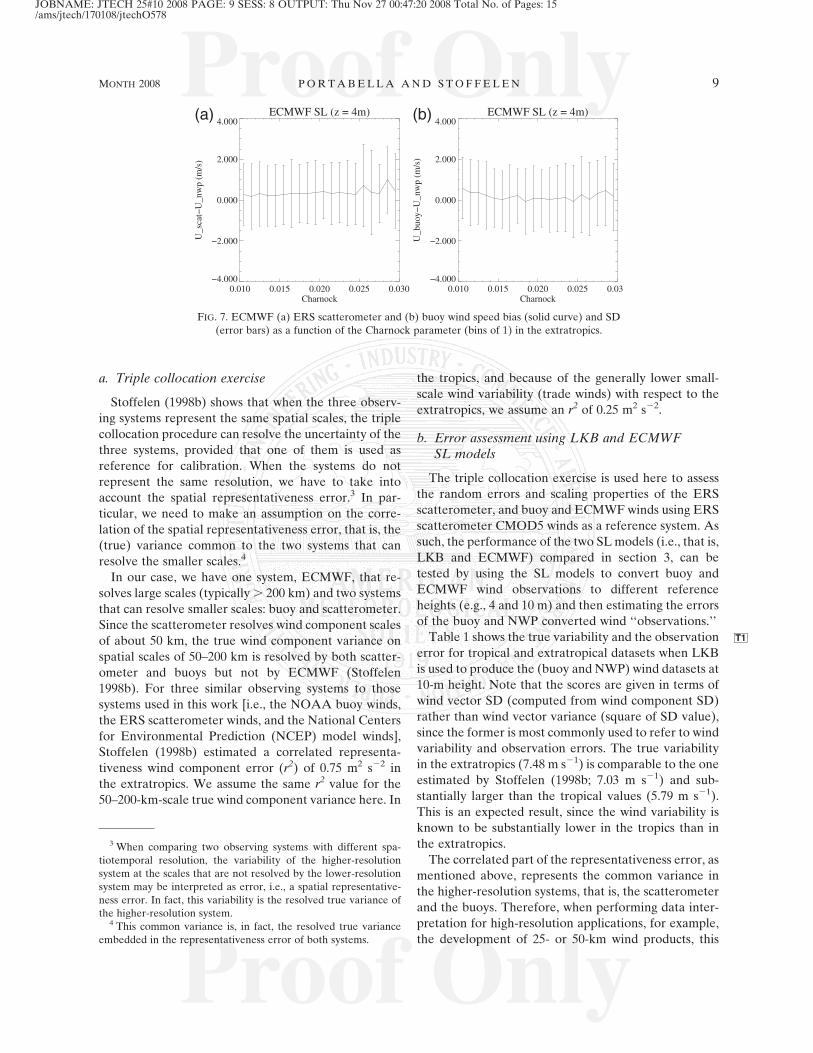
Figure 7 shows the F7scatterometer–ECMWF (Fig. 7a)

and buoy–ECMWF (Fig. 7b) speed bias and SD as a

function of the Charnock parameter in the extratropics.

As in Fig. 6, ECMWF and GTS buoy speeds have been

converted to 4-m height speeds using the ECMWF SL

model. Since the scatterometer actually observes sea

surface roughness, which is directly affected by the

wave-induced stress, we would expect that for increas-

ing Charnock (sea state) values, sea surface roughness

and, therefore, the mean biases in the left plot would

FIG. 3. Same as Fig. 2b but for the estimated z0 parameter.

FIG. 4. Normalized histogram of z/L for both the LKB model

(solid line) and the ECMWF SL model (dotted line), using the

extratropical ECMWF dataset as input. Negative, null, and posi-

tive z/L values correspond to unstable, neutral, and stable strati-

fication, respectively.

FIG. 5. Same as Fig. 2b but with variable Charnock input to the

ECMWF SL model.



Proof Only

Proof Only

increase. However, the bias is rather flat and very sim-

ilar to the one in the right plot, where for the same set of

points no explicit roughness effect is expected. More-

over, the spread in the data points could be different as a

result of sea state effects, which is also not the case as

the plots look very similar indeed. The wind vector cell

(WVC) mean sea state roughness as observed by scat-

terometers thus appears mainly wind driven and cases

of substantial stress–wind decoupling appear excep-

tional. The slight bias increase at large Charnock values

in the left panel may be an indication of stress–wind

decoupling, although there is not enough data to sup-

port this statement. It is, therefore, concluded that, in

general, Charnock is very much correlated to the WVC-

mean wind (see Fig. 6) and, therefore, has a small im-

pact on the quality of a global SOS.2 However, the

Charnock parameter may contain some added value for

exceptional conditions, such as cases of extreme wind

variability and/or air–sea temperature difference. A

much larger dataset is needed, however, to further in-

vestigate this value.

4) ATMOSPHERIC STABILITY EFFECTS

The impact of stability on wind stress estimates is

often measured by the difference between the actual

wind (U) and its equivalent neutral wind (Un), that is,

the wind that results from estimating u*, given a wind

observation at certain height z and under certain at-

mospheric stability (z/L), and subsequently using such

u* to solve Eq. (2) at the same height z assuming neutral

stability (i.e., c 5 0).

Figure 8 shows the F8difference between Un and U as a

function of U using the LKB model for the tropical (left

panel) and extratropical (right panel) buoy input data-

sets. In the tropics (Fig. 8a), differences between neutral

winds and actual wind tend to increase for low winds

(below 3 m s21) and then slightly decrease for increasing

speeds. In the extratropics (Fig. 8b), this pattern is less

evident as a result of the presence of a wider range of

stratification (stronger stable and unstable situations),

although still present. The same pattern is produced

when using ECMWF SL model instead of LKB and/or

ECMWF input instead of buoy input (not shown). It is

clear from Fig. 8 that stability effects are small both in

the tropics and the extratropics and generally within the

range [0, 0.3] m s21.

4. Wind-to-stress characterization

In remote sensing, validation or calibration activities

can only be done properly when the full error charac-

teristics of the data are known. In practice, the problem

is that prior knowledge on the full error characteristics

is seldom available. Stoffelen (1998b) shows that si-

multaneous error modeling and calibration can be

achieved by using triple collocations. Simultaneous er-

ror modeling and calibration can be used to compare

triple collocation wind component datasets. In this

section, the scatterometer winds are fixed in all datasets

and used as reference. The two other wind-observing

systems (i.e., buoys and NWP) are presented at varying

heights and stability conditions, such that the true and

error variances can be evaluated for the different da-

tasets. In this way, the interpretation of the different

observing systems and the performance of the SL

models are characterized in this section.

FIG. 6. Charnock parameter mean value (solid curve) and SD (error bars) as a function of (a) ERS

scatterometer and (b) ECMWF wind speed (bins of 1 m s21) in the extratropics.

2 Note that same conclusions are drawn when repeating the

same exercise using calibrated (see section 4) scatterometer winds.



Proof Only

Proof Only

a. Triple collocation exercise

Stoffelen (1998b) shows that when the three observ-

ing systems represent the same spatial scales, the triple

collocation procedure can resolve the uncertainty of the

three systems, provided that one of them is used as

reference for calibration. When the systems do not

represent the same resolution, we have to take into

account the spatial representativeness error.3 In par-

ticular, we need to make an assumption on the corre-

lation of the spatial representativeness error, that is, the

(true) variance common to the two systems that can

resolve the smaller scales.4

In our case, we have one system, ECMWF, that re-

solves large scales (typically . 200 km) and two systems

that can resolve smaller scales: buoy and scatterometer.

Since the scatterometer resolves wind component scales

of about 50 km, the true wind component variance on

spatial scales of 50–200 km is resolved by both scatter-

ometer and buoys but not by ECMWF (Stoffelen

1998b). For three similar observing systems to those

systems used in this work [i.e., the NOAA buoy winds,

the ERS scatterometer winds, and the National Centers

for Environmental Prediction (NCEP) model winds],

Stoffelen (1998b) estimated a correlated representa-

tiveness wind component error (r2) of 0.75 m2 s22 in

the extratropics. We assume the same r2 value for the

50–200-km-scale true wind component variance here. In

the tropics, and because of the generally lower small-

scale wind variability (trade winds) with respect to the

extratropics, we assume an r2 of 0.25 m2 s22.

b. Error assessment using LKB and ECMWFSL models

The triple collocation exercise is used here to assess

the random errors and scaling properties of the ERS

scatterometer, and buoy and ECMWF winds using ERS

scatterometer CMOD5 winds as a reference system. As

such, the performance of the two SL models (i.e., that is,

LKB and ECMWF) compared in section 3, can be

tested by using the SL models to convert buoy and

ECMWF wind observations to different reference

heights (e.g., 4 and 10 m) and then estimating the errors

of the buoy and NWP converted wind ‘‘observations.’’

Table 1 shows the T1true variability and the observation

error for tropical and extratropical datasets when LKB

is used to produce the (buoy and NWP) wind datasets at

10-m height. Note that the scores are given in terms of

wind vector SD (computed from wind component SD)

rather than wind vector variance (square of SD value),

since the former is most commonly used to refer to wind

variability and observation errors. The true variability

in the extratropics (7.48 m s21) is comparable to the one

estimated by Stoffelen (1998b; 7.03 m s21) and sub-

stantially larger than the tropical values (5.79 m s21).

This is an expected result, since the wind variability is

known to be substantially lower in the tropics than in

the extratropics.

The correlated part of the representativeness error, as

mentioned above, represents the common variance in

the higher-resolution systems, that is, the scatterometer

and the buoys. Therefore, when performing data inter-

pretation for high-resolution applications, for example,

the development of 25- or 50-km wind products, this

FIG. 7. ECMWF (a) ERS scatterometer and (b) buoy wind speed bias (solid curve) and SD

(error bars) as a function of the Charnock parameter (bins of 1) in the extratropics.

3 When comparing two observing systems with different spa-

tiotemporal resolution, the variability of the higher-resolution

system at the scales that are not resolved by the lower-resolution

system may be interpreted as error, i.e., a spatial representative-

ness error. In fact, this variability is the resolved true variance of

the higher-resolution system.4 This common variance is, in fact, the resolved true variance

embedded in the representativeness error of both systems.



Proof Only

Proof Only

common variance is considered as part of the true

variance but also as part of the error (lack of high-

resolution information) of the lower-resolution system,

that is, the NWP model.T2 Table 2 provides accounts for

such interpretation. On the other hand, when looking at

lower-resolution applications—for example, NWP data

assimilation—this common variance cannot be resolved

and is, therefore, interpreted as part of the (spatial

representativeness) error of the higher-resolution systems,

that is, scatterometer and buoy. Note that Table 1 shows

the same as Table 2, but it accounts for the latter in-

terpretation. We also note that differences between the

two tables are produced by the assumed r2 value, which

is small compared to true variance and generally modest

compared to the error variances.

When the ECMWF SL model is used (instead of

LKB) to produce the (buoy and NWP) wind datasets at

10-m height, the triple collocation results (not shown)

are almost identical to the ones in Tables 1 and 2, that is,

the performance of both SL models is comparable.

These results are in line with the results of section 3,

where both models were showing little differences. The

same exercise is repeated using buoy and NWP winds at

4-m height (the approximate measurement height of

buoys). In this case, no SL model transformation is re-

quired for the buoy winds. The results (not shown) are

very similar in terms of true variability and errors of the

different sources, denoting that the SL model does not

introduce additional error when buoy winds are trans-

formed from 4 to 10 m. It also implies that scatterometer

winds can be scaled equally well to 10- and 4-m winds.

However, when performing triple collocation, the

scaling factor for buoy (i.e., the buoy-to-scatterometer

wind calibration value) is closer to one at a reference

height of 4 than at 10 m, meaning that CMOD5 scat-

terometer winds should be interpreted as 4- winds

rather than 10-m winds.

c. Scatterometer wind interpretation

As discussed in the introduction, scatterometers are

essentially observing wind stress. Therefore, we may

better interpret scatterometer-derived winds as equiv-

alent neutral winds (i.e., stress) rather than real winds.TABLE 1. Estimates of the wind vector SD of the true distribu-

tion and the errors of the scatterometer, LKB-derived 10-m buoy

and ECMWF winds for NWP-scale (;200 km) wind in the tropics

and the extratropics.

True wind Scatterometer Buoy ECMWF

Tropics (m s21) 5.79 1.36 1.63 1.91

Extratropics (m s21) 7.48 2.01 1.98 1.78

TABLE 2. Same as in Table 1, but for 50-km-scale wind.


Tropics (m s21) 5.84 1.17 1.48 2.04

Extratropics (m s21) 7.58 1.60 1.55 2.16

FIG. 8. Difference between the LKB estimated Un and U as a function of U for (a) TAO/PIRATA

(tropics) and (b) GTS (extratropics) buoy input datasets at 4-m height. Note that points from (b) plot

have been perturbed along the x-axis bins with a uniform distribution ranging [20.5, 0.5] m s21 to better

discern the vertical distribution of points, i.e., the GTS speed binning (see section 2), otherwise it pro-

duces a concentration of points along the vertical lines.



Proof Only

Proof Only

In this section, we investigate the interpretation of

scatterometer data by performing the triple collocation

exercise for the following two different datasets:

d ERS CMOD5 winds, buoy real winds, and ECMWF

real winds; andd ERS CMOD5 winds, buoy neutral winds, and

ECMWF neutral winds.

The first dataset is the same as the one used in sec-

tion 4b. The second dataset is the same as the first one

but for buoy and NWP-converted neutral winds using

either the LKB or ECMWF SL model. As in section 4b,

ERS scatterometer CMOD5 winds are used as reference.

The true variability and error scores of dataset A (see

Tables 1 and 2) are very similar to the scores obtained

with dataset B (seeT3 Tables 3 and 4) when using LKB

modelT4 and 10-m conversion. The same conclusions are

drawn when using the ECMWF SL model and/or 4-m

conversion. This indicates that scatterometer winds can

explain the same true variability regardless of whether

these are tested against real or neutral winds. That is,

scatterometer winds are as representative of real winds

as they are of equivalent neutral winds (or stress).

To reinforce such conclusion, and given the fact that

CMOD5 GMF was tuned to 10-m real (NWP) winds, we

develop a new GMF (CMOD5n) by tuning our CMOD5

real winds to neutral winds.F9 Figure 9 shows the bias of

CMOD5 winds with respect to 10-m buoy real winds

(solid) and 10-m buoy neutral winds (dotted) as a

function of buoy wind speed.5 By subtracting these two

curves [i.e., about 0.2 m s21 in the tropics (Fig. 9a) and

0.1 m s21 in the extratropics (Fig. 9b)], we derive a

statistical real-to-neutral conversion (dashed) that can

be used to derive CMOD5n from CMOD5.

We then perform the same triple collocation exercise

as before but using ERS CMOD5n winds instead of

CMOD5 winds in datasets A and B as a reference. As

expected, the results are, again, very similar.

The fact that scatterometer winds are statistically as

close to real winds as to neutral winds can be explained

as follows. On the one hand, the stability effects are

small, that is, differences between real and neutral

winds are subtle (see Fig. 8 in section 3b). On the other

hand, SL models and the different observations (wind,

SST, and air temperature) used by the models to com-

pute height conversions and neutral winds contain er-

rors, which in turn mask the already subtle differences

between real and neutral winds (Stoffelen et al. 2006;

Portabella and Stoffelen 2007).

Although scatterometer winds can be interpreted as

real winds from a statistical point of view, there may be

special air–sea interaction situations where the scatter-

ometer shows its real potential to measure stress. For

example, note that a difference of 0.2 m s21 exists be-

tween neutral and real winds using the tropical dataset.

The extratropical difference (0.1 m s21) is smaller

mainly because of cases with stable stratification that

appear below the main cloud of points in Fig. 8. For

these single cases, the use of stability information may

increase the true variability in a triple collocation ex-

ercise, therefore indicating that such scatterometer ob-

servations should be interpreted as neutral winds (or

stress) rather than real winds. To prove this, further

tests with a larger dataset are required.

d. Scatterometer wind-to-stress transformation

To obtain stress, first a well-calibrated scatterometer

10-m neutral wind is required. Then an SL model like

the LKB or ECMWF SL can be used to convert 10-m

neutral winds to wind stress. In fact, since the most re-

cently developed SL models (Taylor and Yelland 2001;

Bourassa 2006) have similar performance up to 16 m s21

(Bourassa 2006), either one of them can be used to do

the neutral-to-stress conversion. Because no stability

information is needed to do this conversion, an inde-

pendent SOS product can be developed straightfor-

wardly.

To obtain the calibrated scatterometer 10-m neutral

wind, a scatterometer-to-buoy correction (calibration)

and a real-to-neutral wind conversion need to be ap-

plied to CMOD5 winds. The combined correction and

conversion is represented by the dotted curves in Fig. 9,

which have a different mean (absolute) value of 0.8

m s21 in the tropics (Fig. 9a) and 0.55 m s21 in the ex-

tratropics (Fig. 9b). The latter further confirms the results

from Hersbach et al. (2007) with a similar extratropical

dataset.

TABLE 3. Estimates of the wind vector SD of the true distribu-

tion and the errors of the scatterometer, LKB-derived 10-m buoy

and ECMWF neutral winds for NWP-scale (;200 km) wind in the

tropics and the extratropics.


Tropics (m s21) 5.79 1.37 1.64 1.92

Extratropics (m s21) 7.49 1.97 2.01 1.78

TABLE 4. Same as in Table 3, but for 50-km-scale wind.


Tropics (m s21) 5.83 1.17 1.48 2.04

Extratropics (m s21) 7.59 1.54 1.60 2.16

5 Since most of the times there is unstable stratification (see Fig. 4),

the real winds are biased low with respect to the equivalent neutral

winds at any reference height within the SL.



Proof Only

Proof Only

Several effects may lead to these differences between

tropical and extratropical datasets. The most relevant

effects are, on the one hand, the large wind variability in

the extratropics and, on the other hand, the effect of

currents in the tropics. To recommend a final combined

correction value, an analysis of the uncertainties of the

triple collocation exercise (mainly produced by the

mentioned effects) is performed. One way to analyze

such uncertainties is to take the calibrated dataset (after

triple collocation) and examine the residual biases buoy

by buoy. As such, we compute the residual wind com-

ponent (the west–east U and the south–north V wind

components) buoy and ECMWF biases against scat-

terometer at each buoy location.T5 Table 5 shows the

average and SD of the mentioned wind component re-

sidual biases. Only buoy locations with at least 50 triple

collocations—34 tropical and 30 extratropical buoy

locations—are used in the statistics. The uncertainty

found in the extratropics (SD of about 0.2 m s21) is

consistent with the expected wind variability effect. A

comparable result is found for the tropical dataset, in-

dicating that the uncertainties produced by, for exam-

ple, the currents in the tropics, are comparable to the

ones produced by, for example, the large wind varia-

bility in the extratropics. In other words, for a global

correction both combined correction values (i.e., 0.8

m s21 found in the tropics and 0.55 m s21 in the extra-

tropics) have a similar degree of confidence.

Therefore, we recommend adding 0.7 m s21 (com-

promise between the tropical and the extratropical

values) to CMOD5 winds to obtain the scatterometer

10-m neutral winds. To obtain real winds we recom-

mend adding 0.5 m s21 to CMOD5.

5. Conclusions

Scatterometer backscatter is closely related to ocean

kinematic stress. For practical reasons, however, C-

band backscatter has been related to real 10-m winds.

Effects of stability, currents, and waves could then po-

tentially cause error in the scatterometer interpretation.

In this paper, we statistically investigate a physically

more direct interpretation of scatterometer backscatter

data as kinematic stress or as its equivalent 10-m neutral

winds.

Since direct stress or roughness measurements are

generally lacking for such purpose, a tropical and an

extratropical triple-collocated wind dataset are used:

ERS-2 scatterometer winds, moored buoy data, and

ECMWF model output. As a consequence, all com-

parisons are based on a fixed set of data points and

uncertainties as a result of a difference in the number or

FIG. 9. Relative bias of CMOD5 winds with respect to 10-m buoy real winds (solid line) and 10-m buoy

neutral winds (dotted line) as a function of buoy wind speed for the (a) tropical and (b) extratropical

datasets. The buoy height conversion is performed with the LKB model. The dashed curve corresponds to

the solid minus the dotted curve. The thick solid curve corresponds to the number of data.

TABLE 5. Average and SD of the wind component residual biases (after wind calibration) for buoy and ECMWF winds against

scatterometer winds in the tropics/extratropics.

Buoy scat. U component Buoy scat. V component ECMWF scat. U component ECMWF scat. V component

Avg (m s21) 0.09 / 0.03 20.02 / 20.12 0.21 / 0.08 20.02 / 20.06

SD (m s21) 0.27 / 0.16 0.13 / 0.24 0.27 / 0.26 0.22 / 0.24



Proof Only

Proof Only

location (e.g., by screening) of the inputs are absent.

That is, the geophysical conditions for the comparisons

are set fixed and a careful geophysical analysis follows.

First, a comparison between two commonly used SL

models, LKB and ECMWF, is performed. The main

difference between the two models is in the roughness

length (z0) and the stability (L) parameterizations. LKB

uses a constant Charnock value, ECMWF uses a sub-

stantially larger Charnock value. Since the ECMWF

roughness parameterization is sea state dependent, its

Charnock parameter is also variable, particularly in

the extratropics. However, LKB has larger instability

(larger negative z/L values) with respect to ECMWF.

This difference actually compensates for the difference

in the roughness formulation for moderate winds, such

that the resulting stress values are very similar for both

models. At high winds though, the stability term is much

smaller than the roughness term and, therefore, the

different roughness formulation results in some small

stress bias (about 5%) between the two models.

Another relevant result of this comparison is that sea

state–dependent (variable Charnock) effects are small

and that the atmospheric stability effects are also small

and of the order of ocean current effects. Otherwise, the

results show similar performance of both SL models.

To characterize the ability of scatterometers to mea-

sure stress and wind, two triple collocation exercises are

performed: the first one uses scatterometer CMOD5

winds together with buoy and NWP real winds; the

second one uses the same data but buoy and NWP

neutral winds instead, where neutral winds are a mea-

sure of the SL stress. True variability and error scores

are almost identical in both exercises, meaning that

scatterometer winds are as close to real winds as to

neutral winds, provided that we use the appropriate

scaling. A test with scatterometer neutral winds further

corroborates such interpretation. An explanation for

the duality in scatterometer data interpretation is that

the small stability effects are masked by the uncertainty

in SL models and their inputs.

The results presented in this paper confirm the ones

obtained by Hersbach et al. (2007) with a similar ex-

tratropical dataset. As such, we confirm that an inde-

pendent ERS scatterometer stress (SOS) product can

be obtained by adding 0.7 m s21 to CMOD5 winds and

use this result as the 10-m neutral wind input to a re-

cently developed SL model, which is needed to compute

stress. [Note that KNMI uses the LKB SL model, since

it is widely used and publicly available.] A schematic

illustration of the wind-to-stress conversion is shown in

Fig. 10 F10.

The formulation of the roughness length [Eq. (3)]

presented by these two SL models is not the only one

available. Differences between different formulations

have been thoroughly studied. For example, Bonekamp

et al (2002) claim that a wave age–dependent Charnock

SL model (such as ECMWF) is marginally better than

a constant Charnock model (such as LKB). Moreover,

several authors have proposed different wave age–

dependent parameterizations, for example, Donelan

(1990), Maat et al. (1991), Smith et al. (1992), Johnson

et al. (1998), and Drennan et al. (2003). On the other

FIG. 10. Schematic of recommended scatterometer wind and stress conversion. The well-validated

CMOD5 winds at 10-m height are used as basis for geophysical conversion to friction velocity. Either real

or neutral 10-m winds may be transformed to friction velocity by either LKB, ECMWF, or any similar SL

model.



Proof Only

Proof Onlyhand, Taylor and Yelland (2001) proposed an alterna-

tive wave steepness parameterization of z0. The work

presented in section 4 could be used to compare the

performance of additional SL models in interpreting

scatterometer measurements.

However, in general, SL model differences in terms of

wind stress magnitude are small for winds below 10

m s21, and it is only well above 10 m s21 that the dif-

ferent roughness formulations produce large differences

in the estimated stress (see also Taylor et al. 2001).

Moreover, according to Bourassa (2006), the most re-

cently developed SL models (e.g., Taylor and Yelland

2001; Bourassa 2006) have similar performance up to 16

m s21, which is consistent with the comparison of LKB

and ECMWF SL models performed in here. However,

cases of extreme wind variability or air–sea temperature

difference may show large wind and stress discrep-

ancies. The triple-collocated datasets used in this paper

are not sufficient to properly investigate the perfor-

mance of the SL models in such extreme cases, where

the differences between models may be more signifi-

cant. As such, a study over a much larger dataset is

recommended for such purposes. Moreover, it would

also be interesting to study the ability of scatterometers

to measure stress in such extreme conditions.

Although the results in this paper relate to the ERS

scatterometer, the wind-to-stress conversion also ap-

plies to other scatterometers. A new C-band scatter-

ometer, that is, the Advanced Scatterometer [(ASCAT)

on board the Meteorological Operation (MetOp)],

which has more than twice the coverage of the ERS

scatterometer, was launched on 19 October 2006. In the

framework of a collaboration between NOAA and

EUMETSAT, ASCAT underflights have been planned

during the NOAA 2007 winter storm and tropical cy-

clone campaigns. These extreme weather datasets could,

therefore, be used for the above-mentioned purposes.

Acknowledgments. Special thanks go to Jean-

Raymond Bidlot and ECMWF for providing the GTS

buoy dataset (already quality controlled) together with

feedback on the collocation exercise and our results. We

acknowledge the help and collaboration of our col-

leagues working at KNMI, and specifically the people

from the scatterometer group. This work is funded by

the European Organization for the Exploitation of

Meteorological Satellites (EUMETSAT) Climate

Monitoring (CM) and Ocean and Sea Ice (OSI) Satellite

Application Facilities (SAFs), led by the Deutscher

Wetterdienst (DWD) and Meteo-France, respectively.

The software used in this work was developed at KNMI,

through the EUMETSAT OSI and numerical weather

prediction (NWP) SAFs, and at ECMWF. We greatly

appreciate the three reviewers who helped to improve

this paper.

REFERENCES

Attema, E. P. W., 1991: The active microwave instrument on board

the ERS-1 satellite. Proc. IEEE, 79, 791–799.

Beljaars, A. C. M., 1997: Air–sea interaction in the ECMWF

model. Proc. Seminar on Atmosphere–Surface Interaction,

Reading, United Kingdom, ECMWF, 33–52.

Bidlot, J.-R., D. J. Holmes, P. A. Wittmann, R. Lalbeharry, and

H. S. Chen, 2002: Intercomparison of the performance of

operational ocean wave forecasting systems with buoy data.

Wea. Forecasting, 17, 287–310.

Bonekamp, H., G. J. Komen, A. Sterl, P. A. E. M. Janssen, P. K.

Taylor, and M. J. Yelland, 2002: Statistical comparisons of

observed and ECMWF modelled open ocean surface drag.

J. Phys. Oceanogr., 32, 1010–1027.

Bourassa, M. A., 2006: Satellite-based observations of surface

turbulent stress during severe weather. Atmosphere–Ocean

Interactions, Volume 2, W. Perrie, Ed., Advances in Fluid

Mechanics, Vol. 39, WIT Press, 35–52.

Brown, A. R., A. C. M. Beljaars, H. Hersbach, A. Hollingsworth,

M. Miller, and D. Vasiljevic, 2005: Wind turning across the

marine atmospheric boundary layer. Quart. J. Roy. Meteor.

Soc., 131, 1233–1250, doi:10.1256/qj.04.163.

Businger, J. A., 1973: Turbulent transfer in the atmospheric sur-

face layer. Workshop on Micrometeorology, D. H. Haugen,

Ed., Amer. Meteor. Soc., 67–100.

Charnock, H., 1955: Wind stress on a water surface. Quart. J. Roy.

Meteor. Soc., 81, 639–640.

Chelton, D. B., and M. G. Schlax, 1996: Global observations of

oceanic Rossby waves. Science, 272, 234–238.

——, and Coauthors, 2001: Observations of coupling between

surface wind stress and sea surface temperature in the eastern

tropical Pacific. J. Climate, 14, 1479–1498.

——, M. G. Schlax, M. H. Freilich, and R. F. Millif, 2004: Satellite

measurements reveal persistent small-scale features in ocean

winds. Science, 303, 978–983.

Donelan, M. A., 1990: Air–sea interaction. Ocean Engineering

Science, B. Le Mehaute and D. M. Hanes, Eds., The Sea Se-

ries, Vol. 9, John Wiley, 239–292.

——, F. W. Dobson, S. D. Smith, and R. J. Anderson, 1993: On the

dependence of sea surface roughness on wave development.

J. Phys. Oceanogr., 23, 2143–2149.

Drennan, W. M., H. C. Graber, D. Hauser, and C. Quentin, 2003:

On the wave age dependence of wind stress over pure wind

seas. J. Geophys. Res., 108, 8062, doi:10.1029/2000JC000715.

Geernaert, G. L., 1999: Theory of air–sea momentum, heat and gas

fluxes, Air–Sea Exchange: Physics, Chemistry, and Dynamics,

G. L. Geernaert, Ed., Kluwer Academy Publishers, 25–48.

Hersbach, H., A. Stoffelen, and S. de Haan, 2007: The improved

C-band ocean geophysical model function: CMOD-5. J. Ge-

ophys. Res., 112, C03006, doi:10.1029/2006JC003743.

Janssen, P., 2004: The Interaction of Ocean Waves and Wind.

Cambridge University Press, 300 pp.

Johnson, H. K., J. Højstrup, H. J. Vested, and S. E. Larsen, 1998:

On the dependence of sea surface roughness on wind waves.

J. Phys. Oceanogr., 28, 1702–1716.

Kelly, K. A., S. Dickinson, M. J. McPhaden, and G. C. Johnson,

2001: Ocean currents evident in satellite wind data. Geophys.

Res. Lett., 28, 2469–2472.



Proof Only

Proof OnlyLiu, W. T., and W. Tang, 1996: Equivalent neutral wind. Jet Pro-

pulsion Laboratory Tech. Rep. 96-17, 22 pp.

——, K. B. Katsaros, and J. A. Businger, 1979: Bulk parameteri-

zation of air–sea exchanges of heat and water vapor including

the molecular constraints at the interface. J. Atmos. Sci., 36,

1722–1735.

Maat, N., C. Kraan, and W. A. Oost, 1991: The roughness of wind

waves. Bound.-Layer Meteor., 54, 89–103.

Milliff, R. F., 2005: Forcing global and regional ocean numerical

models with ocean surface vector winds from spaceborne

observing systems. Satellite Application Facility (SAF)

Training Workshop: Second Workshop on Ocean and Sea Ice,

EUMETSAT Rep. P.45, 8 pp.

——, and J. Morzel, 2001: The global distribution of the time-

average wind stress curl from NSCAT. J. Atmos. Sci., 58,109–131.

Monin, A. S., and A. M. Obukov, 1954: Basic regularity in tur-

bulent mixing in the surface layer of the atmosphere. Tr.

Geofiz. Inst., Akad. Nauk SSSR, 24, 163–187.

Portabella, M., and A. Stoffelen, 2007: Development of a global

scatterometer validation and monitoring. EUMETSAT

Ocean and Sea Ice SAF Scientific Rep. SAF/OSI/CDOP/

KNMI/SCI/RP/141, 37 pp.

Smith, S. D., and Coauthors, 1992: Sea surface wind stress and drag

coefficients: The HEXOS results. Bound.-Layer Meteor., 60,

109–142.

Stoffelen, A., 1996: Error modeling of scatterometer, in-situ, and

ECMWF model winds: A calibration refinement. KNMI Tech.

Rep. 193, 44 pp.

——, 1998a: Scatterometry. Ph.D. thesis, University of Utrecht,

195 pp.

——, 1998b: Error modeling and calibration: Towards the true

surface wind speed. J. Geophys. Res., 103 (C4), 7755–7766.

——, 2002: Scatterometer Ocean Stress. Proposal to the CM-SAF,

KNMI. xxx pp. [Available online at http://www.knmi.nl/

scatterometer/.] AU3

——, 2008: Scatterometer applications in the European Seas, Re-

mote Sensing of the European Seas, V. Barale and M. Gade,

Eds., Springer, 269–282.

——, A., G. J. van Oldenborgh, J. de Kloe, M. Portabella, and A.

Verhoef, 2006: Development of a scatterometer ocean stress

product. EUMETSAT Climate Monitoring SAF Rep., 66 pp.

Taylor, P. K., and M. J. Yelland, 2001: The dependence of sea

surface roughness on the height and steepness of the waves.

J. Phys. Oceanogr., 31, 572–590.

——, ——, and E. C. Kent, 2001: On the accuracy of ocean winds

and wind stress. WCRP/SCOR Workshop on Intercompari-

son and Validation of Ocean–Atmosphere Flux Fields,

WCRP Rep. 115, XXX pp AU4.

Vialard, J., 2000: Seasonal forecast and its requirements for sat-

ellite products. Ocean and Sea Ice SAF Training Workshop,

EUMETSAT Rep. P27, 137–143.



On Scatterometer Ocean Stress

Documents

Transcript of On Scatterometer Ocean Stress