The following ad supports maintaining our C.E.E.O.L. service 

 

 

SUBSAMPLING APPROACH FOR STATISTICAL INFERENCE WITHINSTOCHASTIC DEA MODELS

«SUBSAMPLING APPROACH FOR STATISTICAL INFERENCE WITHINSTOCHASTIC DEA MODELS»

by Artur Prędki

Source:Quantitave Methods in Economics (Metody Ilościowe w Badaniach Ekonomicznych), issue: XIV­2 /2013, pages: 158­168, on www.ceeol.com.

QUANTITATIVE METHODS IN ECONOMICS

Vol. XIV, No. 2, 2013, pp. 158 – 168

SUBSAMPLING APPROACH FOR STATISTICAL INFERENCE 1

WITHIN STOCHASTIC DEA MODELS1 2

Artur Prędki 3 Department of Econometrics and Operations Research 4

Cracow University of Economics 5 e-mail: predkia@uek.krakow.pl 6

Abstract: In the current literature, many different stochastic extensions of the 7 DEA framework can be found. Such generalized approaches enable one to 8 model the uncertainty inherent to the form of the production possibility set 9 and the value of the technical efficiency measure at any given point of the 10 former. In the paper we provide a detailed discussion of some statistical 11 model and the subsampling algorithm which are used in statistical inference. 12 The methodology is then illustrated with an empirical example using the real-13 world data from the Polish energy sector. 14

Keywords: DEA method, technical efficiency, statistical inference, 15 subsampling 16

INTRODUCTION 17

Essentially, data envelopment analysis (or DEA, in short) is applied to 18 measure technical efficiency within a group of n production (or, more generally, 19 decision-making) units producing s sorts of outputs (arrayed in vector 20 yj = [y1j, …, ysj] for j = 1, …, n) out of m sorts of inputs (xj = [x1j, …, xmj]). 21

In what follows we assume that the producers are technologically 22 homogenous and the technology itself is represented by the production set T, the 23 specifics of which are discussed in the following section. Additionally, in 24 a deterministic DEA framework, T is specified as a minimal set (in terms 25 of inclusion), containing all the data points (xj, yj), j = 1, …, n. Such an approach 26

1 Research conducted under financial support from Cracow University of Economics. The

author would like to express his gratitude to Dr Łukasz Kwiatkowski for his assistance

with English translation of the paper.

Access via CEEOL NL Germany

Subsampling approach for statistical inference … 159

enables one to derive its form explicitly. On the other hand, such an assumption is 1 invalid within stochastic variations of DEA, which is attributable to uncertainty 2 inherent to the data collected2. Consequently, the production set is of an unknown 3 form. 4

Based on T, the so-called Farrell technical efficiency measure (for some 5 feasible production plan (xo, yo)) can be defined. Such a measure underlies studies 6 employing DEA methods and is usually formulated in the input- and output-7 oriented settings, respectively: 8

(xo, yo) = min{ R: (xo, yo) T}, 9 (xo, yo) = max{ R: (xo, yo) T}. 10

In the research we restrict ourselves to the input orientation solely. 11 In a deterministic DEA framework, owing to a known form of the production set, 12 a unique value of the measure can be calculated by solving appropriate linear 13 programs (see, e.g., [Guzik 2009]). However, it is no longer the case in stochastic 14 DEA methods, where the actual form of T remains unknown. 15

STATISTICAL MODEL 16

In the paper we focus on one of the stochastic DEA methods, developed by 17 a team of researchers gathered around Professor Léopold Simar3. According to the 18 preceding remarks, the setting requires the form of T to be approximated, so that 19 technical efficiency measure can be further estimated at any given point of T. For 20 the approximation and estimation to be valid one needs to formulate a relevant 21 model. In the present study we resort to the methodology presented by Kneip et al. 22 [2008], recognized for its transparency as compared with earlier suggestions found 23 in the literature (see [Kneip et al. 1998], [Gijbels et al. 1999] and [Park et al. 24 2000]). 25

Below we present three most fundamental assumptions that are material to 26 further considerations, starting with the one specifying properties of the production 27 set. 28 Assumption 1. The units produce s sorts of goods out of m sorts of inputs and use 29 the same technology, represented by T – a closed and convex production set, 30 satisfying the ‘free disposal’ (or: inefficiency) condition and the ‘no free lunch’ 31 condition (i.e. no output can be produced out of zero inputs). 32 For more details and a review of other possible properties of the production set we 33 refer to, e.g., [Prędki 2012]. 34

The second assumption pertains to the data generating process. 35

2 The uncertainty may arise as a result of measurement errors or data incompleteness, for

instance. 3 Léopold Simar (born 1946) is Full Professor of Statistics at the Department of Statistics,

Université Catholique de Louvain (Belgium).

160 Artur Prędki

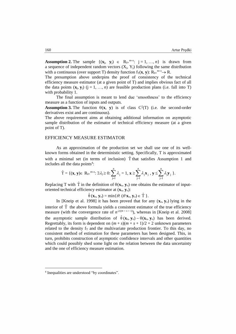
Assumption 2. The sample {(xj, yj) R0+m+s: j = 1, …, n} is drawn from 1

a sequence of independent random vectors (Xj, Yj) following the same distribution 2 with a continuous (over support T) density function fT(x, y): R0+

m+s R. 3 The presumption above underpins the proof of consistency of the technical 4 efficiency measure estimator (at a given point of T) and implies obvious fact of all 5 the data points (xj, yj) (j = 1, …, n) are feasible production plans (i.e. fall into T) 6 with probability 1. 7

The final assumption is meant to lend due ‘smoothness’ to the efficiency 8 measure as a function of inputs and outputs. 9 Assumption 3. The function (x, y) is of class C2(T) (i.e. the second-order 10 derivatives exist and are continuous). 11 The above requirement aims at obtaining additional information on asymptotic 12 sample distribution of the estimator of technical efficiency measure (at a given 13 point of T). 14

EFFICIENCY MEASURE ESTIMATOR 15

As an approximation of the production set we shall use one of its well-16 known forms obtained in the deterministic setting. Specifically, T is approximated 17

with a minimal set (in terms of inclusion) T that satisfies Assumption 1 and 18 includes all the data points4: 19

T = {(x, y) R0+m+s: j 0:

n

1j

j = 1, x

n

1j

jjx , y

n

1j

jjy }. 20

Replacing T with T in the definition of (xo, yo) one obtains the estimator of input-21 oriented technical efficiency estimator at (xo, yo): 22

θ (xo, yo) = min{: ( xo, yo) T }. 23 In [Kneip et al. 1998] it has been proved that for any (xo, yo) lying in the 24

interior of T the above formula yields a consistent estimator of the true efficiency 25 measure (with the convergence rate of n-2/(m + s + 1)), whereas in [Kneip et al. 2008] 26

the asymptotic sample distribution of θ (xo, yo) (xo, yo) has been derived. 27 Regrettably, its form is dependent on (m + s)(m + s + 1)/2 + 2 unknown parameters 28 related to the density fT and the multivariate production frontier. To this day, no 29 consistent method of estimation for these parameters has been designed. This, in 30 turn, prohibits construction of asymptotic confidence intervals and other quantities 31 which could possibly shed some light on the relation between the data uncertainty 32 and the one of efficiency measure estimation. 33

4 Inequalities are understood “by coordinates”.

Subsampling approach for statistical inference … 161

BOOTSTRAP 1

In the situation outlined above, one is prompted to resort to the bootstrap 2 methods, which have gained much favor since the late 1990s. Such an approach, 3 based on simulating additional samples out the original one, allow for 4 approximation of the aforementioned confidence intervals and some measures of 5 statistical dispersion. A necessary condition for any bootstrap procedure to be valid 6 is its consistency, which requires (in the limiting case of n) the distribution of 7 the bootstrap estimator of an efficiency measure to be corresponding (in a certain 8 manner) with the actual asymptotic distribution of the estimator considered in the 9 previous section. A formal definition of the bootstrap consistency can be found in, 10 e.g., [Simar and Wilson 2000, p. 61]. It seems that early attempts of designing 11 relevant bootstrap procedures (such as the ones presented in [Löthgren and 12 Tambour 1999], [Simar and Wilson 1998, 2000]) have not been quite successful as 13 they have resulted in either methods consistency of which could not be formally 14 verified, or in ones proved positively inconsistent5. Moreover, some of these have 15 been founded upon a quite restrictive and non-verifiable assumption of 16 homogeneity of technical efficiency measure. Only recently, in [Kneip et al. 2008], 17 have two consistent bootstrap methods been devised. However, one of them 18 requires solving a huge number of linear programs at each bootstrap iteration, 19 which renders the method (already complex due to its multilevelness and intricate 20 formulae) computationally formidable. Therefore, the other of the two – resting 21 upon the idea of the so-called subsampling – seems a more attractive alternative. 22

SUBSAMPLING 23

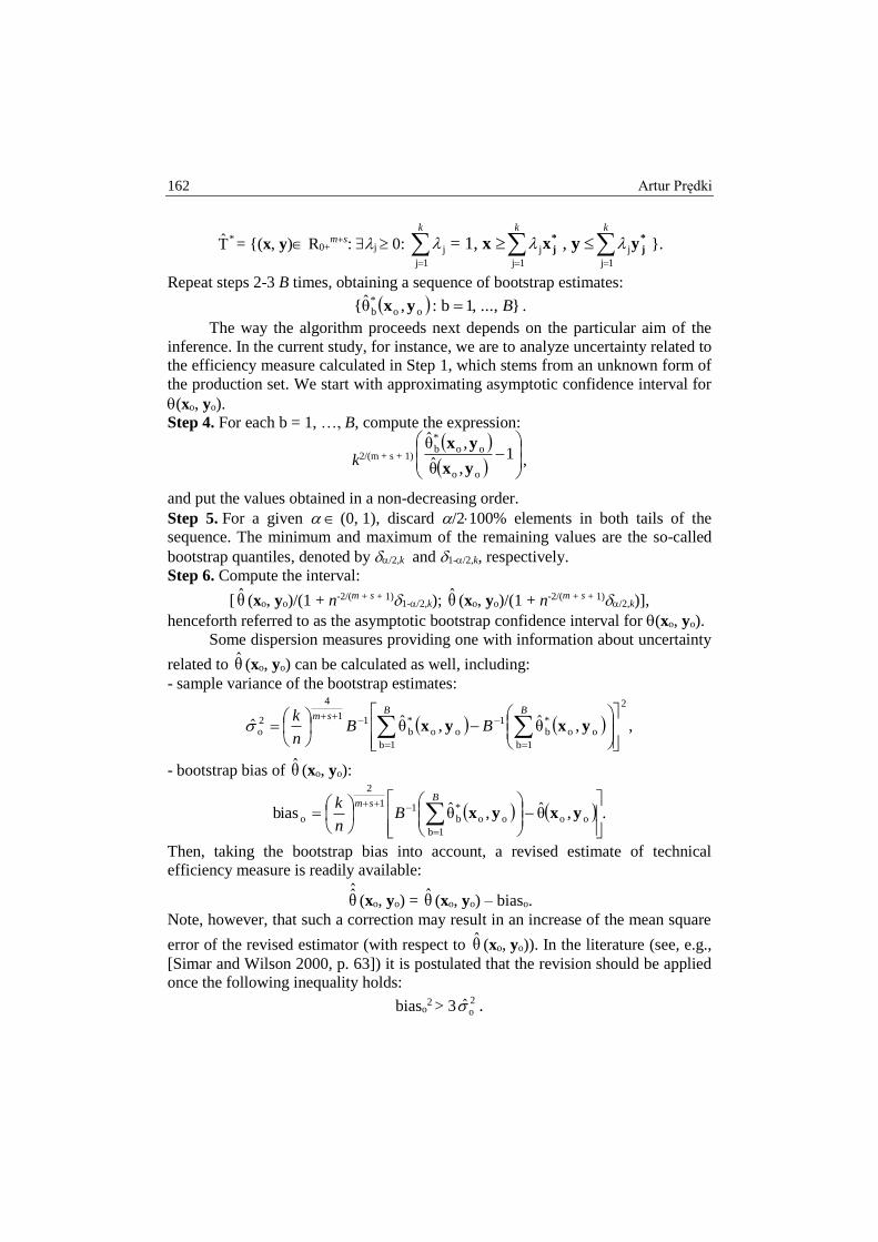
Since the subsampling approach is the one employed in our empirical study 24 to follow, we present in some more detail the way the method proceeds. 25

Step 1. Based on the original sample, the value of θ (xo, yo) is calculated. 26 Step 2. Generate a bootstrap sample {(xj

*, yj*): j = 1, …, k} by randomly drawing 27

(independently, uniformly, and with replacement) k < n observations from the 28 original sample6. 29 Step 3. The bootstrap estimate of (xo, yo) is computed according to the formula: 30

oo* ,θ yx = min{: ( xo, yo)

*T }, 31

where 32

5 Only some simulation studies have been carried out, the results of which seem to

corroborate consistency of some procedures (under a given Data Generating Process). 6 While specifying value of k = k(n) in simulation studies one needs to guarantee that

k(n) and k(n)/n0 in the limiting case of n. Assuming k = n (which corresponds

with the so-called naive bootstrap) results in inconsistency of the procedure.

162 Artur Prędki

*T = {(x, y) R0+m+s: j 0:

k

1j

j = 1, x

k

1j

j*jx , y

k

1j

j*jy }. 1

Repeat steps 2-3 B times, obtaining a sequence of bootstrap estimates: 2

}...,,1b:,θ{ oo*b Byx . 3

The way the algorithm proceeds next depends on the particular aim of the 4 inference. In the current study, for instance, we are to analyze uncertainty related to 5 the efficiency measure calculated in Step 1, which stems from an unknown form of 6 the production set. We start with approximating asymptotic confidence interval for 7 (xo, yo). 8 Step 4. For each b = 1, …, B, compute the expression: 9

k2/(m + s + 1)

1

,θ

,θ

oo

oo*b

yx

yx, 10

and put the values obtained in a non-decreasing order. 11 Step 5. For a given (0, 1), discard /2100% elements in both tails of the 12 sequence. The minimum and maximum of the remaining values are the so-called 13 bootstrap quantiles, denoted by /2,k and 1-/2,k, respectively. 14 Step 6. Compute the interval: 15

[ θ (xo, yo)/(1 + n-2/(m + s + 1)1-/2,k); θ (xo, yo)/(1 + n-2/(m + s + 1)/2,k)], 16

henceforth referred to as the asymptotic bootstrap confidence interval for (xo, yo). 17 Some dispersion measures providing one with information about uncertainty 18

related to θ (xo, yo) can be calculated as well, including: 19 - sample variance of the bootstrap estimates: 20

,,θ,θˆ

2

1b

oo*b

1

1b

oo*b

11

4

2o

BB

smBB

n

kyxyx 21

- bootstrap bias of θ (xo, yo): 22

.,θ,θbias oo

1b

oo*b

11

2

o

yxyx

Bsm

Bn

k 23

Then, taking the bootstrap bias into account, a revised estimate of technical 24 efficiency measure is readily available: 25

θˆ

(xo, yo) = θ (xo, yo) – biaso. 26 Note, however, that such a correction may result in an increase of the mean square 27

error of the revised estimator (with respect to θ (xo, yo)). In the literature (see, e.g., 28 [Simar and Wilson 2000, p. 63]) it is postulated that the revision should be applied 29 once the following inequality holds: 30

biaso2 > 3

2o . 31

Subsampling approach for statistical inference … 163

SPECIFIC PROBLEMS 1

While using the DEA methods, values of the efficiency measure are 2 calculated for each of the units in the original sample, i.e. for o = 1, …, n, as it is 3 the main objective of the approach to compare and rank the units with respect to 4 their efficiency. Analogously, one may wish to obtain (approximated) confidence 5 intervals and the dispersion measures for each unit. However, theoretical results 6 and simulation studies presented in the relevant literature (see [Kneip et al. 2008] 7 and [Simar and Wilson 2011]) consider only a single object (xo, yo) that is assumed 8 to be independent of the ones in the original sample {(xj, yj) R0+

m+s: j = 1, …, n}7. 9 Aiming at employing the subsampling approach in order to compute the confidence 10 intervals and dispersion measures we slightly modify the procedure outlined above. 11 We proceed along some hints found in [Simar and Wilson 2011, p. 40]. Firstly, the 12 subsampling procedure is repeated n times for each o = 1, …, n. For a given unit, 13 the algorithm proceeds similarly as before with the only modification in Step 2, 14 now consisting in drawing k out of n – 1 elements (excluding object o). Naturally, 15 in such a case k < n – 1, so some information is lost, yet the required independence 16 is guaranteed. 17

Choosing an appropriate value for k is another key issue. Some simulation 18 studies carried out in [Kneip et al. 2008] indicate a critical role of the parameter to 19 final results of the subsampling procedure, thereby proving their pronounced 20 sensitivity. Nevertheless, no universal approach (featuring some desired statistical 21 properties) to selecting the ‘right’ number for k can be pointed. Therefore, we 22 resort to (quite an arbitrary) empirical rule that has been formulated in [Simar and 23 Wilson 2011, pp. 42-43]. The method – presented below – is a particular version 24 of a general procedure designed in [Politis et al. 2001], and has specifically been 25 developed to deal with approximation of confidence intervals. 26 Step 1. For a given point (xo, yo), conduct the subsampling scheme for arbitrarily 27 specified values of k: k1 < k2 < … < kW. As a result one obtains a sequence 28 of corresponding confidence intervals:{[L(kw); R(kw)]: w = 1, …, W}. 29 Step 2. Choose some arbitrary small natural number v (usually, in practice, 30 v assumes the value of one, two or three). 31 Step 3. For any w [v + 1, W v],calculate a sum of standard deviations of the 32 left-hand side endpoints: L(kwv),…, L(kw+v), and of the right-hand side ones: 33 R(kwv), …, R(kw+v). 34 Step 4. For a given w [v + 1, W v], select the value of kw {k1, k2, …, kW} that 35 minimizes the sum computed in Step 3. 36

7 In the sense of the random vector (Xo, Yo) being stochastically independent of each

(Xj, Yj), j = 1, …, n.

164 Artur Prędki

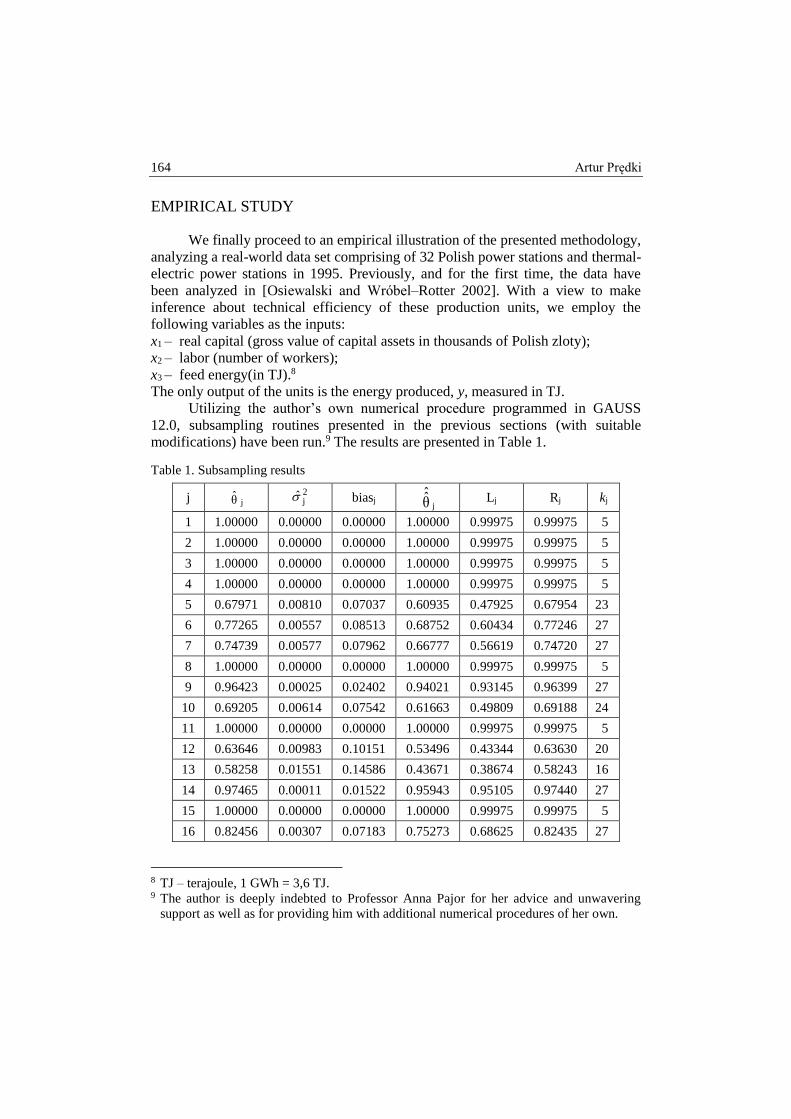
EMPIRICAL STUDY 1

We finally proceed to an empirical illustration of the presented methodology, 2 analyzing a real-world data set comprising of 32 Polish power stations and thermal-3 electric power stations in 1995. Previously, and for the first time, the data have 4 been analyzed in [Osiewalski and Wróbel–Rotter 2002]. With a view to make 5 inference about technical efficiency of these production units, we employ the 6 following variables as the inputs: 7 x1 – real capital (gross value of capital assets in thousands of Polish zloty); 8 x2 – labor (number of workers); 9 x3 – feed energy(in TJ).8 10 The only output of the units is the energy produced, y, measured in TJ. 11

Utilizing the author’s own numerical procedure programmed in GAUSS 12 12.0, subsampling routines presented in the previous sections (with suitable 13 modifications) have been run.9 The results are presented in Table 1. 14

Table 1. Subsampling results 15

j θ j

2j biasj θ

ˆj

Lj Rj kj

1 1.00000 0.00000 0.00000 1.00000 0.99975 0.99975 5

2 1.00000 0.00000 0.00000 1.00000 0.99975 0.99975 5

3 1.00000 0.00000 0.00000 1.00000 0.99975 0.99975 5

4 1.00000 0.00000 0.00000 1.00000 0.99975 0.99975 5

5 0.67971 0.00810 0.07037 0.60935 0.47925 0.67954 23

6 0.77265 0.00557 0.08513 0.68752 0.60434 0.77246 27

7 0.74739 0.00577 0.07962 0.66777 0.56619 0.74720 27

8 1.00000 0.00000 0.00000 1.00000 0.99975 0.99975 5

9 0.96423 0.00025 0.02402 0.94021 0.93145 0.96399 27

10 0.69205 0.00614 0.07542 0.61663 0.49809 0.69188 24

11 1.00000 0.00000 0.00000 1.00000 0.99975 0.99975 5

12 0.63646 0.00983 0.10151 0.53496 0.43344 0.63630 20

13 0.58258 0.01551 0.14586 0.43671 0.38674 0.58243 16

14 0.97465 0.00011 0.01522 0.95943 0.95105 0.97440 27

15 1.00000 0.00000 0.00000 1.00000 0.99975 0.99975 5

16 0.82456 0.00307 0.07183 0.75273 0.68625 0.82435 27

8 TJ – terajoule, 1 GWh = 3,6 TJ. 9 The author is deeply indebted to Professor Anna Pajor for her advice and unwavering

support as well as for providing him with additional numerical procedures of her own.

Subsampling approach for statistical inference … 165

j θ j

2j biasj θ

ˆj

Lj Rj kj

17 0.82574 0.00283 0.05880 0.76694 0.68825 0.82553 27

18 1.00000 0.00000 0.00000 1.00000 0.99975 0.99975 5

19 0.96811 0.00016 0.01122 0.95689 0.93864 0.96786 27

20 0.95963 0.00021 0.02988 0.92974 0.92272 0.95939 27

21 0.65916 0.00217 0.06664 0.59252 0.54118 0.65899 19

22 0.62917 0.00411 0.06698 0.56219 0.47174 0.62901 25

23 1.00000 0.00000 0.00000 1.00000 0.99975 0.99975 5

24 0.86040 0.00338 0.06460 0.79581 0.74578 0.86019 27

25 0.81771 0.00221 0.04918 0.76853 0.67515 0.81751 27

26 0.75999 0.00506 0.05942 0.70057 0.58505 0.75980 27

27 0.75424 0.00629 0.06550 0.68875 0.57647 0.75405 27

28 0.89069 0.00190 0.04488 0.84582 0.79796 0.89047 27

29 1.00000 0.00000 0.00000 1.00000 0.99975 0.99975 5

30 1.00000 0.00000 0.00000 1.00000 0.99975 0.99975 5

31 1.00000 0.00000 0.00000 1.00000 0.99975 0.99975 5

32 1.00000 0.00000 0.00000 1.00000 0.99975 0.99975 5

Source: own elaboration 1

In columns 2-4 of Table 1 we report estimates obtained for the measure 2 of efficiency and measures of its dispersion, whereas in columns 5-7 – the revised 3 estimates of the efficiency measure along with approximated asymptotic 4 confidence intervals (with Lj and Rj standing for the left- and the right-hand side 5 endpoints, respectively). The last column displays values of kj’s, i.e. the number 6 of generated bootstrap samples for each data point (xj, yj) (j = 1, …, n), which have 7 been specified according to the empirical rule discussed in the previous section.10 8

As regards selecting particular values for B and v, we follow the mainstream 9 literature and set B = 2000 and v = 2, which obviously does not shed the 10 arbitrariness of such a choice. Reflecting on specific choices for k, again, we 11 resorted to general suggestions found in the literature and – avoiding extreme 12 possible values of the parameter – considered k {3, 4, …, 29}. Since n = 32 in 13 our study, setting k close to 32 would imply slower convergence due to the 14 algorithm “nearing” the (inconsistent) naive bootstrap (see Footnote 6). On the 15 other hand, low values of the parameter result in a sizeable loss of information and 16 enforce low number of bootstrap subsamples available to be generated. 17

10 Let us recall that the bootstrap samples generated for any j do not include the unit itself.

166 Artur Prędki

According to values reported in the last column of Table 1, it is clear that 1 following the empirical rule discussed above the most frequent choice for the 2 number of elements in a subsample is 27. With regard to revision of the point 3 estimates of the efficiency measure, only in the case of unit j = 20 the relevant 4 inequality holds so that the correction is then justified.11 Values of the bias-revised 5 estimator for the other units are presented only for the sake of completeness. 6

Estimates of the efficiency measures hover between 0.586 and 1.000. The 7 lowest efficiency is indicated for unit j = 13, whereas power stations no.: 1-4, 8, 11, 8 15, 18, 23, 29-32, appear to be the most efficient. Note, however, that the 9 subsampling procedure is not valid for the latter, as it was not possible to obtain 10 either non-zero values of the dispersion measures or reasonable approximations 11 of the confidence intervals. On a technical note, it is caused by a lack of objects 12 with a higher value of the efficiency measure in the original sample. Partly, it is 13 also in accord with the theoretical results discussed above, which hold only for the 14 data points lying in the interior of the production set, thereby lacking in efficiency. 15 Admittedly, one cannot dismiss a possibility that our estimates of technical 16 efficiency are incorrect and that the units may in fact be inefficient. Nevertheless, 17 with the data set in hand it is not possible to diagnose conclusively whether it is 18 actually the case. 19

For the units that emerged to be inefficient we managed to compute both the 20 bootstrap measures of dispersion as well as approximated confidence intervals. 21 One needs to perceive the results with some caution, however, as the low number 22 of units in the sample undermines the asymptotics. 23

Table 2 presents relative and absolute measures of dispersion (only for the 24 inefficient stations), sorted increasingly with respect to technical efficiency 25 estimates.12 26 27

11 See the end part of the “Subsampling” section. 12 As an absolute measure of dispersion we consider the diameter of a confidence interval,

i.e. Rj Lj, the values of which are reported in the last column of Table 2.

Subsampling approach for statistical inference … 167

Table 2. Relative and absolute measures of dispersion 1

j θ j jj θσ biasj/ θ j Rj Lj

13 0.58258 0.21380 0.25038 0.195692

22 0.62917 0.101879 0.106458 0.157266

12 0.63646 0.15575 0.15949 0.202866

21 0.65916 0.070723 0.101093 0.117812

5 0.67971 0.13243 0.10353 0.200289

10 0.69205 0.11327 0.10898 0.193788

7 0.74739 0.10166 0.10654 0.181013

27 0.75424 0.10517 0.08684 0.177587

26 0.75999 0.09364 0.07818 0.17475

6 0.77265 0.09656 0.11018 0.168121

25 0.81771 0.05749 0.06015 0.14236

16 0.82456 0.06721 0.08711 0.138101

17 0.82574 0.06441 0.07121 0.137282

24 0.86040 0.06754 0.07508 0.114401

28 0.89069 0.04894 0.05039 0.09251

20 0.95963 0.015051 0.031142 0.03667

9 0.96423 0.01654 0.02491 0.032538

19 0.96811 0.01289 0.01159 0.029225

14 0.97465 0.01083 0.01561 0.023352

Source: own elaboration 2

Note a clear negative correlation between estimates of efficiency measure 3

and its dispersion. It follows that higher values of jθ are usually accompanied with 4

tighter confidence intervals. Conversely, for units of lesser efficiency higher 5 uncertainty is typically indicated. A technical reason behind that observation 6 resides in the fact that the generated subsamples contain a large fraction of highly 7 efficient units, with respect to which the highly inefficient ones are compared. It 8 should be pointed, however, that values obtained for the relative dispersion 9 measures do not exceed 25% of the point estimate. Therefore, even for the most 10 inefficient power stations the relative uncertainty is not considerable. 11

REFERENCES 12

Gijbels I., Mammen E., Park B.U., Simar L. (1999) On estimation of monotone and 13 concave frontier function, JASA, Vol. 94, pp. 220-228. 14

168 Artur Prędki

Guzik B. (2009) Basic DEA models in analysis of economic and social efficiency, Poznań 1 University of Economics, Poznań. 2

Kneip A., Park B.U., Simar L. (1998) A Note on the convergence of nonparametric DEA 3 estimators for production efficiency scores, Econometric Theory, Vol. 14, pp. 783-793. 4

Kneip A., Simar L., Wilson P.W. (2008) Asymptotics and consistent bootstraps for DEA 5 estimators in nonparametric frontier models, Econometric Theory, Vol. 24, pp. 1663-6 1697. 7

Löthgren M., Tambour M. (1999) Testing scale efficiency in DEA models: a bootstrapping 8 approach, Applied Economics, Vol. 31, pp. 1231-1237. 9

Osiewalski J., Wróbel–Rotter R. (2002) A Bayesian Random Effect Model in Cost 10 Efficiency Analysis (with the Application to Polish Electric Power Stations), Statistical 11 Review, Vol. 49(2), pp. 47-68. 12

Park B.U., Simar L., Weiner Ch. (2000) The FDH estimator for productivity efficiency 13 scores, Econometric Theory, Vol. 16, pp. 855-877. 14

Politis D., Romano J., Wolf M. (2001) On the asymptotic theory of subsampling, Statistica 15 Sinica, Vol. 11, pp. 1105-1124. 16

Prędki A. (2012) The Origins of Production Possibility Sets in the DEA Method [in:] 17 Mathematics and Information Technology at the Service of Economics: Theory - 18 Models, [ed.] W. Jurek, Scientific Bulletin of Poznań University of Economics, no. 241, 19 Poznań, pp. 126-137. 20

Simar L., Wilson P.W. (1998) Sensitivity analysis of efficiency scores: how to bootstrap in 21 nonparametric frontier models, Management Science, Vol. 44, pp. 49-61. 22

Simar L., Wilson P.W. (2000) A general methodology for bootstrapping In nonparametric 23 frontier models, Journal of Applied Statistics, Vol. 27, pp. 779-802. 24

Simar L., Wilson P.W. (2011) Inference by the m out of n bootstrap in nonparametric 25 frontier models, Journal of Productivity Analysis, Vol. 36, pp. 33-53. 26