Applying Data Envelopment Analysis (DEA) toOptimize the Fertilizer and Pesticides Consumptionin Wetland Rice Cultivation in MalaysiaModather Mairghany  ( fayoomy1974@gmail.com )

University Putra Malaysia https://orcid.org/0000-0003-3566-0626Suha Elsoragaby 

University Putra MalaysiaAzmi Yahya 

University Putra MalaysiaNor Maria Adam 

University Putra MalaysiaMohamad Firdza Mohamad Shukery 

University Putra Malaysia

Research Article

Keywords: Technical E�ciency, Pure Technical E�ciency, E�cient farm, Optimum Amount, Input Oriented,Output Oriented

Posted Date: August 1st, 2022

DOI: https://doi.org/10.21203/rs.3.rs-1893180/v1

License: This work is licensed under a Creative Commons Attribution 4.0 International License.  Read Full License

1

Applying Data Envelopment Analysis (DEA) to Optimize the Fertilizer and 1

Pesticides Consumption in Wetland Rice Cultivation in Malaysia 2

Modather Mairghany*1, 2, Suha Elsoragaby

1, 3, Azmi Yahya1, Nor Maria Adam4, and Mohamad Firdza 3

Mohamad Shukery1 4

1Dept. of Biological and Agricultural Engineering, Faculty of Engineering, University Putra Malaysia 5

Dept. of Chemical Engineering, Faculty of Engineering, Red Sea University, Port Sudan, Sudan 6 3Dept. of Agricultural and Biological Engineering, Faculty of Engineering, University of Khartoum, 7

Khartoum, Sudan 8 4Dept. of Mechanical Engineering, Faculty of Engineering, 43400 Serdang, Selangor D.E. 9

1Email address of the corresponding author: fayoomy1974@gmail.com 10

Abstract 11

Fertilizers and pesticides are the most effective and costly inputs in rice production in wetland rice 12

cultivation in Malaysia. Farmers need to know the optimum amount of these inputs to produce the 13

same rice yield. In this study, Data Envelopment Analysis (DEA) was used to estimate the farm 14

input efficiencies of rice production based on seven inputs including N, P, K, and chemicals 15

pesticides liquid insecticides, solid insecticides, fungicides, and herbicides, and one output of rice 16

grain yield. The study aimed to benchmark the inefficient farms to the efficient farms to optimize 17

the fertilizer and pesticide inputs, and also maximize the rice grain yield output. We used three 18

main models Charnes–Cooper–Rhodes (CCR), Banker–Charnes–Cooper (BCC), and Slacks-19

Based Measure (SBM) models in both direction input and output-oriented to evaluate the 20

performance of every model and determine the effective one. The technical, pure technical, scale 21

and cross efficiencies were calculated for rice production through the three models. The results 22

revealed the average technical were (0.89 and 0.95) for CCR, (0.76 and 0.87) for SBM-I-C, (0.89 23

and 0.95) for SBM-O-C, and pure technical efficiencies were (0.95 and 0.97) for BCC-I, (0.97 and 24

0.99) for BCC-O, (0.79 and 0.9) for SBM-I-V, and (0.96 and 0.99) for SBN-O-V for first and 25

second season respectively. The results showed that out of the total number of farms the efficient 26

2

farms were 16.7% and 43.3% for CCR models, and 26.7% and 56.7% for BCC models for the first 27

and second season respectively. 28

Keywords: Technical Efficiency; Pure Technical Efficiency; Efficient farm, Optimum Amount; 29

Input Oriented; Output Oriented. 30

1. Introduction 31

Data envelopment analysis DEA is used as a method and approach to analyzing the performance 32

of farms to determine which farms are efficient in terms of using inputs resources and giving output 33

and that not efficient mainly those who use more input and give lesser output. DEA analyze and 34

compare the performance between farms and benchmark the inefficient farms to the efficient ones, 35

using the benchmark techniques aim to show the farmers how to improve their performance for 36

inefficient farms by following the same method for the efficient farms (Aung, 2012). The basic 37

performance of data envelopment analysis is to find and calculate the technical efficiency of the 38

farms which is called here by the decision-making unit DMU, and this efficiency is expressed as 39

the ratio of the summation of weighted outputs to the summation of the weighted inputs, and 40

normally it ranges from zero to one. Technical efficiency represents the ability of a farm to achieve 41

high efficiency by either minimizing the input resources and/or maximizing output. If the technical 42

efficiency value equals one, that means the DMU is efficient in its resource use and if it is lesser 43

than 1 it indicates an inefficient situation that needs more improvement in terms of resource 44

utilization and maximization of the yielded output. 45

In data envelopment analysis DEA, the analyzed target is called Decision Making Unit DMUs, 46

these DMUs are a producer using and utilizing different levels of resource inputs, and producing 47

different levels of outputs may be single or multiple outputs based on the producer working 48

method. The DEA tries to identify which DMUs are most effective while at the same time 49

3

indicating specific deficiencies of other producers or DMUs (Nassiri & Singh 2009). There are 50

several variants of the data envelopment analysis DEA model, but there are two of which are most 51

commonly used known as constant return to scale (CRS) models and variable return to scale (VRS) 52

models. The discriminatory power for the constant return to scale CRS model is much higher when 53

compared to the variable return to scale VRS model. 54

Many researchers used data envelopment analysis DEA in the agricultural production sector: 55

Chauhan et al. (2006) used (DEA) to measure and improve the productivity of energy in rice 56

production in India. Nassiri and Singh (2009) used the DEA to measure the farmers' efficiencies 57

in terms of energy use in rice production in India. Mousavi-Avval et al. (2011) used data 58

envelopment analysis DEA to analyze and determine the efficiencies of the framers of apple 59

production in Iran. Mohammadi et al. (2011) used data envelopment analysis DEA to analyze the 60

energy efficiency of kiwifruit production farmers in Iran. Abbas et al., (2018). Mobtaker et al., 61

(2012) used DEA to analyze the efficiency of farmers' use of energy for alfalfa production in Iran. 62

Alizadeh & Taromi (2014) applied the DEA for the optimization of energy consumption in grape 63

production. Khoshnevisan et al. (2013) studied the energy consumption optimization in wheat 64

production, Nabavi- Pelesaraei et al. (2014b) measured the energy efficiencies of orange 65

producers. Elhami et al. (2016) optimized energy consumption for chickpea production. Other 66

researchers used data envelopment DEA to evaluate and analyze the energy consumption by 67

farmers in crop production such as Eyitayo et al. (2011) for cocoa, Banaeian et al. (2011) for 68

greenhouse strawberry, Nabavi-Pelesaraei et al. (2016 b) for watermelon production, Toma et al. 69

(2015) for agricultural, Raheli et al. (2017) for tomato, Qasemi-Kordkheili (2013) for button 70

mushroom, Hosseinzadeh-Bandbafha et al. (2018) for peanut, NabaviPelesaraei et al. (2014c) for 71

tangerine production, Nabavi-Pelesaraei et al. (2014d) in rice. Khoshnevisan et al. (2013) for 72

4

greenhouse cucumber, Mohseni et al. (2018) for grape, Mousavi-Avval et al. (2011b) for soybeans, 73

Mohammadi et al. (2015) for rice, Nabavi- Pelesaraei et al. (2014b) used MOGA and DEA for 74

orange Pahlavan et al. (2012) for greenhouse cucumber and Qasemi-Kordkheili (2015) for 75

grapefruit. 76

For the constant return to scale CRS model, there is a proportional change gain for input and 77

output variables, while for variable return to scale VRS there is no proportional change that 78

gains for input and output variables (Reddy, 2015). The constant return to scale CRS model 79

performs based on constant input or output variable, while the variable return to scale VRS 80

model performs based on increasing or decreasing returns to scale (Tsai & Mar Molinero, 81

2002). CRS model was created by Charnes, Cooper & Rhodes model of DEA and so it was 82

called CCR model or CRS frontier, while the VRS model was created by Banker, Chames, and 83

Cooper and so it was called BCC model or VRS frontier (Benicio & De Mello, 2015; Reddy, 84

2015). The constant return to scale CRS model shows technical efficiency constant, while the 85

VRS model shows pure technical efficiency and scale efficiency which is the difference 86

between VRS and CRS (Kao & Liu, 2011). The constant return to scale CRS model is better 87

in making interpretations, while the variable return to scale VRS model makes complicated 88

interpretations. The third model is the Slacks-Based Measure (SBM) model that was 89

introduced by Tone (2001), this model put aside the assumption of proportionate changes in 90

inputs and outputs and deals with slacks directly. This paper is investigated herein by reference 91

to the CCR, BCC, and SBM models, to determine the optimum amount of fertilizer and pesticide 92

inputs and rice grain yield output. In this paper and to quantify the level of efficiency and 93

inefficiency regarding each of the inputs, the fertilizers including Nitrogen, Phosphorus, and 94

Potassium and pesticide inputs including fungicides, liquid insecticides as insecticides 1, solid 95

5

insecticides as insecticides 2, and herbicides 4 to the rice plant and the rice grain yield output data 96

subjected to Data Envelopment Analysis (DEA). 97

2. Materials and methods 98

2.1. Description of the study area 99

The chosen study area was located in the paddy area (3º29´47´´ N, 101º09 ´56´´ E) in Sungai 100

Burong, Tanjong Karang Kuala Selangor Malaysia. Data were collected for two seasons the first 101

season from June to November 2017 and the second season from January to June 2018. The study 102

was conducted on 30 farms (plots) for two planting seasons. 103

3.5. Ranking the key parameter in improving rice yield/production 104

For ranking the parameters and factors that affect rice production and yield, multiple linear 105

regression analysis was used to determine the most effective factor based on the strongest 106

relationship with a yield based on the value of R2, and R2 adjusted R2 predicted, Whenever R2 107

predicted is higher than means the analysis is very restricted and trusted. 108

A multiple linear regression model with k predictor variables X1, X2... Xk and a response Y can be 109

written as 110

𝑦 = 𝛽0 + 𝛽1𝑥1 + 𝛽2𝑥2 + ··· 𝛽𝐾𝑥𝐾 (28) 111

2.2. Data envelopment analysis (DEA) 112

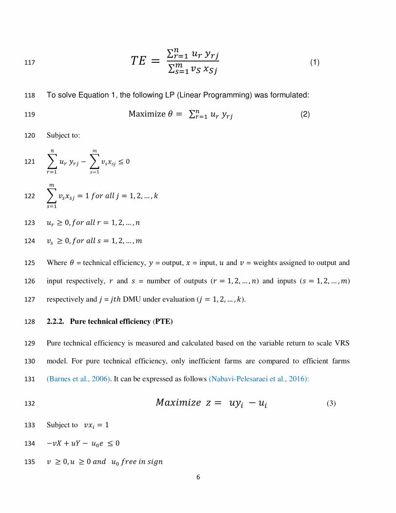
2.2.1. Technical efficiency (TE) 113

Technical efficiency (TE) is measured base on the constant return to scale CRS model it measures 114

the efficiency of any DMU as benchmarked to the efficiency and performance of the other DMU 115

which is represented by the farm. The TE is given in Equation 1 (Nabavi-Pelesaraei et al., 2016): 116

6

𝑇𝐸 = ∑ 𝑢𝑟 𝑦𝑟𝑗𝑛𝑟=1 ∑ 𝑣𝑆 𝑥𝑆𝑗𝑚𝑠=1 (1) 117

To solve Equation 1, the following LP (Linear Programming) was formulated: 118

Maximize 𝜃 = ∑ 𝑢𝑟 𝑦𝑟𝑗𝑛𝑟=1 (2) 119

Subject to: 120

∑ 𝑢𝑟 𝑦𝑟𝑗𝑛𝑟=1 − ∑ 𝑣𝑠𝑥𝑠𝑗 ≤ 0𝑚

𝑠=1 121

∑ 𝑣𝑠𝑥𝑠𝑗 = 1 𝑓𝑜𝑟 𝑎𝑙𝑙 𝑗 = 1, 2, … , 𝑘 𝑚𝑠=1 122

𝑢𝑟 ≥ 0, 𝑓𝑜𝑟 𝑎𝑙𝑙 𝑟 = 1, 2, … , 𝑛 123 𝑣𝑠 ≥ 0, 𝑓𝑜𝑟 𝑎𝑙𝑙 𝑠 = 1, 2, … , 𝑚 124

Where 𝜃 = technical efficiency, 𝑦 = output, 𝑥 = input, 𝑢 and 𝑣 = weights assigned to output and 125

input respectively, 𝑟 and 𝑠 = number of outputs (𝑟 = 1, 2, … , 𝑛) and inputs (𝑠 = 1, 2, … , 𝑚) 126

respectively and 𝑗 = 𝑗𝑡ℎ DMU under evaluation (𝑗 = 1, 2, … , 𝑘). 127

2.2.2. Pure technical efficiency (PTE) 128

Pure technical efficiency is measured and calculated based on the variable return to scale VRS 129

model. For pure technical efficiency, only inefficient farms are compared to efficient farms 130

(Barnes et al., 2006). It can be expressed as follows (Nabavi-Pelesaraei et al., 2016): 131

𝑀𝑎𝑥𝑖𝑚𝑖𝑧𝑒 𝑧 = 𝑢𝑦𝑖 − 𝑢𝑖 (3) 132

Subject to 𝑣𝑥𝑖 = 1 133 −𝑣𝑋 + 𝑢𝑌 − 𝑢0𝑒 ≤ 0 134 𝑣 ≥ 0, 𝑢 ≥ 0 𝑎𝑛𝑑 𝑢0 𝑓𝑟𝑒𝑒 𝑖𝑛 𝑠𝑖𝑔𝑛 135

7

Where z and 𝑢0 are scalar and free in sign; u and v are output and input weight matrixes, and Y 136

and X are the corresponding output and input matrixes, respectively. The letters xi and yi refer to 137

the inputs and output of its DMU. 138

2.2.3. Scale efficiency (SE) 139

Scale efficiency can be expressed as follows (Nabavi-Pelesaraei et al., 2016): 140

𝑆𝑐𝑎𝑙𝑒 𝑒𝑓𝑓𝑖𝑐𝑖𝑒𝑛𝑐𝑦 = 𝑇𝑒𝑐ℎ𝑛𝑖𝑐𝑎𝑙 𝑒𝑓𝑓𝑖𝑐𝑖𝑒𝑛𝑐𝑦𝑃𝑢𝑟𝑒 𝑡𝑒𝑐ℎ𝑛𝑖𝑐𝑎𝑙 𝑒𝑓𝑓𝑖𝑐𝑖𝑒𝑛𝑐𝑦 141

The above linear programming problem (Equation) was solved once for each of the DMUs by first 142

organizing the fertilizers kg/ha and pesticides l/ha or kg/ha inputs and the yield ton/ha outputs data 143

from each farm in the MS-EXCEL software, DEA analysis was made in GAMS using the codes 144

provided in Appendix A. At the same time, MaxDEA 8 Basic 8.3 and DEA-SOLVER-LV8(2014-145

12-05) software were used for the same purpose to compare the accuracy of the result and evaluate 146

the advantages of each software. Segregation between efficient and inefficient farms was made 147

based on their technical efficiency score. Benchmarks were then identified for the inefficient farms 148

and quantification was made on the level of excess inputs they used in the cultivation operations. 149

For the Hybrid distance model we used MaxDEA 8 Basic 8.3 software to run the model, and for 150

Slacks-Based Measure of Efficiency (SBM), we used DEA-SOLVER-LV8(2014-12-05) software. 151

2.3. Statistical Analysis 152

Microsoft Excel 2013 Program was used for computation of mean, standard deviation, the 153

confidence of interval CI and coefficient of variation CV, and also for preparation of graphs. T-154

test and the analysis of variance for various parameters were performed following the ANOVA 155

technique using Minitab Statistical software 18. Pearson's Correlation Coefficient was used as a 156

8

technique for investigating the relationship between two quantitative, continuous variables and 157

measure of the strength of the association between two variables. 158

3. Results and discussion 159

For evaluating and ranking the parameters, the effect of each parameter on rice yield and 160

production was evaluated and ranked using multilinear regression and the parameter was ranked 161

based on the value of R2. The result of the ranking showed that fertilizer was the first key parameter 162

with R2 = 0.83, the second was planting factor with R2 = 0.56, the third factor is pesticide with R2 163

= 0.42 the fourth factor was harvesting with R2 = 0.4, and soil factors with R2 = 0.11. Based on 164

this ranking the data of input of fertilizer and pesticides were subjected to a benchmarking and 165

optimization method, we eliminate the planting factor because the input materials for all plots are 166

the same amount and there were no big differences between them so benchmarking it would not 167

have any effect. 168

The data was collected for two seasons and benchmarking using data envelopment analysis DEA 169

was done for every season separately because the benchmark should be done for plots in the same 170

environment and because the difference in weather status between the two seasons was found 171

significantly different. ANOVA analysis for soil physical properties bulk density, porosity, and 172

penetration resistance showed there was no significant difference between the plots (P ≥ 0.0). The 173

mean amount of materials and sources used including Nitrogen, Phosphorus, and Potassium as 174

fertilizers input kg/ha. The input materials also included pesticides from different sources such as 175

fungicides, liquid insecticides, solid insecticides, and herbicides as l/ha or kg/ha for the solid 176

insecticides. 177

178

9

3.1. Efficiency estimation of farms 179

The summarized statistics results for the three estimated measures of efficiency based on the 180

results of the models CCR and BCC input and output-oriented are shown in Table 1. The results 181

for input-oriented showed that the average technical efficiency, pure technical efficiency, and scale 182

efficiency scores were (89.04 and 95.33%), (94.79 and 97.34%), and (93.97 and 97.87%) for the 183

first and second season respectively. The technical efficiency ranged from 75.25 to 100%, and 184

from 78.98 to 100%, for the first and second seasons respectively. The results for output-oriented 185

showed that the average technical efficiency, pure technical efficiency, and scale efficiency scores 186

were (89.04 and 95.33%), (95.63 and 98.74%), and (93.08 and 96.46%) for the first and second 187

season respectively. The technical efficiency ranged from 75.25 to 100%, and from 78.98 to 100%, 188

for the first and second seasons respectively. 189

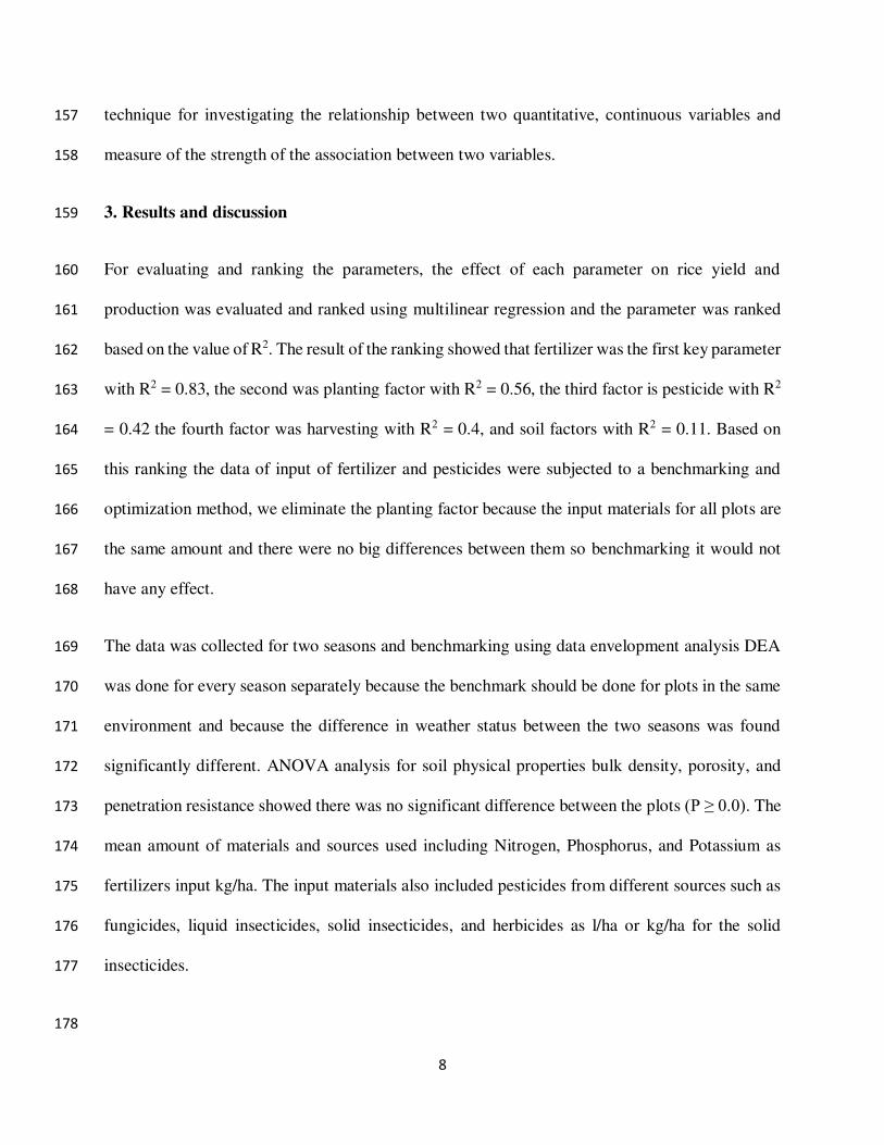
Table 1. Mean technical, pure technical, and scale efficiencies of the farmers for the first season 190

of 2017. 191

Particular Input oriented model Output oriented model

Mean St. Dev. CV Min Max Mean St. Dev. CV Min Max

First season 2017

T. Efficiency 0.89±0.03 0.07 8.14 0.75 1 0.89±0.02 0.07 8.14 0.75 1

P. T. Efficiency 0.95±0.02 0.06 6.17 0.79 1 0.97±0.02 0.05 4.96 0.84 1

Scale Efficiency 0.94±0.02 0.05 5.74 0.86 1 0.93±0.02 0.05 5.74 0.86 1

Second season 2018

T. Efficiency 0.95±0.02 0.07 6.8 0.79 1 0.95±0.02 0.07 6.8 0.79 1

P. T. Efficiency 0.97±0.02 0.05 4.9 0.82 1 0.99±0.01 0.02 2.4 0.91 1

Scale Efficiency 0.98±0.01 0.03 3.2 0.9 1 0.96±0.02 0.05 5 0.85 1

The result of this study revealed that the majority of the farms under analysis are technically 192

inefficient 83.3 and 56.3% for the first and second season respectively, hence there is a greater 193

opportunity and chance for them to improve on their performance by adopting practices of the 194

efficient farms by following the Good Agricultural Practices (MyGap) and the quality of practices 195

and operations in Rice Check. 196

10

3.1.1. Technical efficiency 197

The CCR model contains both technical and scale efficiencies. The efficient results of the CCR-I 198

and CCR-O models are presented in Table 2. For CCR input-oriented or output orient, the results 199

showed no difference in terms of efficient farms for both models input-oriented CCR-I and output-200

oriented CCR-O during the first and second season. From the total of 30 farms considered for the 201

analysis, 5 and 13 farms which equals (16.7 and 43.3%) of the total farms had a technical efficiency 202

score of 1 for the first and second season respectively, and the remaining 25 and 17 farms were 203

inefficient in. About 28 and 64.7% of the inefficient farms had technical efficiency greater than 204

90%, with 72 and 35.3 % of the inefficient farms having an efficiency score of less than 90% for 205

the first and second season respectively. 206

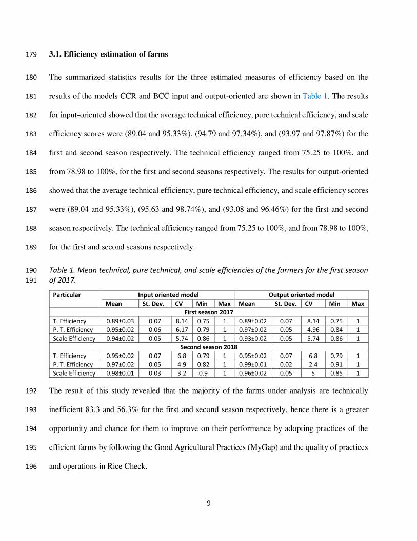
Table 2. Efficient scores distribution of farms for DEA CCR AND BCC models for first and second 207

seasons 2017 and 2018 208

Efficient CCR-I CCR-O BCC-I BCC-O

1st

season

2nd season 1st

season

2nd

season

1st

season

2nd

season

1st

season

2nd

season

1 5 13 5 13 8 17 8 17

90 - 99 7 11 7 11 17 11 17 13

80 -89 16 5 16 5 4 2 5 0

70 -79 2 1 2 1 1 0 0 0

Efficient 5 13 5 13 8 17 8 17

Non-efficient 25 17 25 17 22 13 22 13

Average 0.89 0.95 0.89 0.95 0.95 0.97 0.96 0.99

The mean technical efficiency for all the farms was 89.04 and 95.33%. The outcome of the DEA 209

analysis on the fertilizer and pesticide input and yield output data of the 30 farm plots studied, 210

showed that 7 and 11 farms (53.3 and 16.7%) of farms have efficiencies ranging from 90 to 99% 211

for the first and second seasons respectively. Efficiency from 80 to 89% was achieved by 16 and 212

5 farms (23.3 and 36.7%) of total farms for the first and second season respectively. About 2 and 213

1 farms (6.7 and 3.3%) of the total farms had efficiencies between 70 and 79% for the first and 214

11

second seasons respectively. About 40.0 and 63.3% of the farmers had technical efficiency greater 215

than the mean value for the total farms under study which was 89.04 and 95.33%. 216

3.1.2. Pure technical efficiency 217

The BCC model contains pure technical efficiencies. The efficient results of the BCC-I and BCC-218

O models are presented in Table 2. For BCC input-oriented or output orient, the results showed a 219

difference in terms of efficient farms for both models input-oriented CCR-I and output-oriented 220

CCR-O during the first and second season. From the total of 30 farms under evaluation and 221

analysis and for input orient mode BCC-I, 7 and 17 farms which equals (23.3 and 56.7%) of the 222

total farms had the pure technical efficiency score of 1, while for the output-oriented model BCC-223

O, 8 and 16 farms which equal (26.7 and 53.3%) of the total farms had the pure technical efficiency 224

score of 1, for the first and second season respectively. The remaining 23 and 13 farms (76.67 and 225

43.33%) of the total farms for the input-oriented BCC-I, and 22 and 14 farms (73.33 and 46.67%) 226

of the total farms for output-oriented BCC-O were inefficient in terms of farm inputs utilization in 227

performing the paddy cultivation operations. About 78.26 and 84.62% of the inefficient farms in 228

the input-oriented model BCC-I, and (77.27 and 100%) of the inefficient farms in the output-229

oriented model BCC-O, had pure technical efficiency greater than 90%. 230

About 21.74 and 15.38% of the inefficient farms for the input-oriented model BCC-I, and (22.73 231

and 0%) of the inefficient farms in the output-oriented model BCC-O, had pure technical efficiency 232

scores of less than 90% for the first and second season respectively. The mean pure technical 233

efficiency for all the farms was 94.79 and 97.34% for the input-oriented model BCC-I, and 95.63 234

and 98.74% for the output-oriented model BCC-O, for the first and second season respectively. 235

The result of DEA analysis on the fertilizer and pesticides input and yield output data of the 30 236

farm plots studied, showed that 18 and 11 farms (60.0 and 36.7%) of the total farms for the input-237

12

oriented model BCC-I, 17 and 14 farms (56.7 and 46.7%) of the total farms in the output-oriented 238

model BCC-O, have pure technical efficiencies range from 90 to 99% for first and second season 239

respectively. Efficiency from 80 to 89% was achieved by 4 and 2 farms (13.3 and 6.7%) of total 240

farms for the input-oriented model BCC-I, 5, and 0 farms (16.7 and 0.0%) of the total farms in the 241

output-oriented model BCC-O, for first and second season respectively. About 1 and 0 farms 242

(3.3and 0%) of the total farms for the input-oriented model BCC-I, and no farms in the output-243

oriented model BCC-O, had efficiency between 70 and 79% for the first and second season 244

respectively. 245

Moreover, among the technically efficient farmers 5 and 13 farms (16.7 and 43.3%) had a technical 246

efficiency score of 1 for the first and second season respectively; which indicates that the farmers 247

were globally efficient and were operating at the most productive scale size of production; 248

however, the 8 and 17 pure technically efficient farms for the first and second season respectively, 249

were only locally efficient ones; and that was due to their disadvantageous conditions of scale size. 250

The inefficiency of a farmer comes from two reasons: it is caused by the less quality of farming 251

practices and the worst operation quality of the farm or by the disadvantageous conditions, under 252

which the farmer is operating; so it can be clarified by comparisons of the CCR and BCC efficiency 253

scores. The worst practices quality include choosing the right sources of the resources and 254

materials used and applying the operation at the right timing using the right amount of resources 255

and materials, and placing them in the right places. These practices if the farmers follow can gain 256

high efficiencies and high output quality without wasting resources and materials. 257

Not always the high efficacies could be achieved by reducing the input materials and resources, 258

but also could be achieved through increasing the input resources and materials and also increase 259

the output. Exactly in agriculture, the main principles in increasing the yield are through increase 260

13

fertilizers amount, and also pesticides amount due to the high infestation and damage of pests and 261

diseases, for that we used here both model CCR and BCC, and BCC is the most logical model here 262

due to the concept we mentioned above clarify that if farmers want to increase yield they should 263

use more inputs. 264

3.2.3. Comparison of efficiencies for radial and hybrid model 265

For any individual farm or decision-making unit DMU, the efficiencies of all farms in the radial 266

model were greater than that of hybrid efficiencies except for the efficient ones as it is similar as 267

we mentioned above Figures 1 to 4 show the comparison between radial and hybrid model for 268

technical and pure technical efficiencies for first and second season 2017-2018. Table 3 shows the 269

distribution of technical and pure technical efficiencies for hybrid models. As compared with radial 270

models in Table 2, for efficient farms there were no differences between the models, the same 271

farms were efficient for both models. 272

Table 3. Technical and pure technical efficiency distribution for the hybrid model for the first and second 273

seasons 2017-2018 274

Efficiency SBM-I-C SBM-O-C SBM-I-V SBM-O-V

1st season 2nd season 1st season 2nd season 1st season 2nd season 1st season 2nd season

Efficient 5 13 5 13 8 18 8 17

> 0.9 0 1 7 11 0 0 17 13

> 0.8 1 6 16 5 2 5 5 0

> 0.7 11 7 2 1 10 5 0 0

> 0.6 10 3 0 0 7 2 0 0

> 0.5 3 0 0 0 3 0 0 0

Average 0.76 0.87 0.89 0.95 0.79 0.90 0.96 0.99

The efficient farms in the second season for both models were higher than that in the first season 275

and that is mainly because farmers follow the national standard Rice Check which has a 276

recommendation for the right time, amount, and sources that farmers should use to increase their 277

yields. 278

14

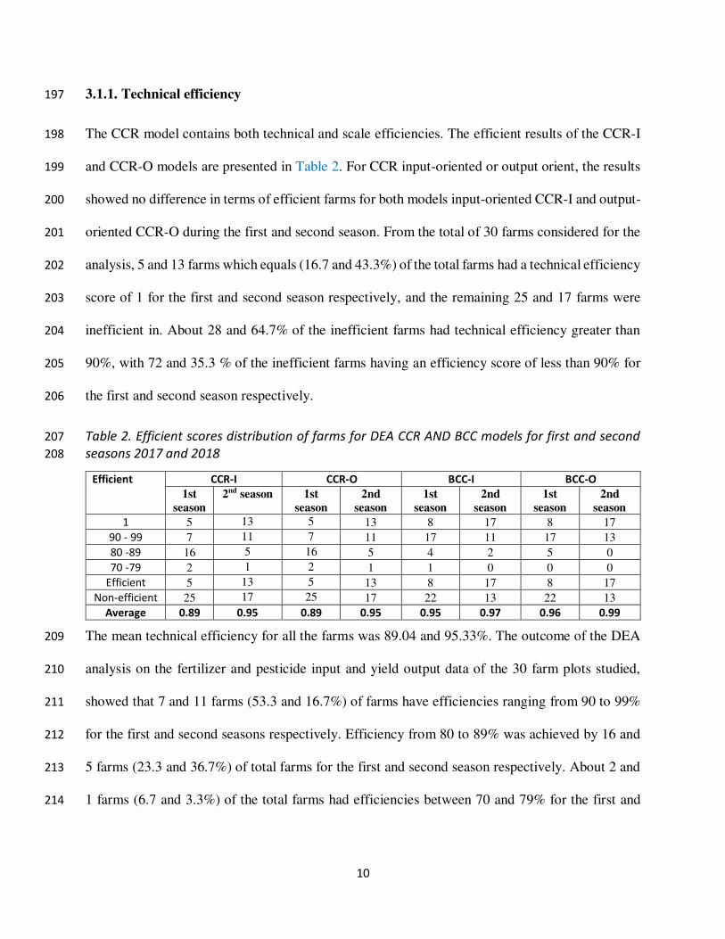
279

Figure 1. Comparison between technical efficiency of CRS radial and hybrid model for the first 280

season 281

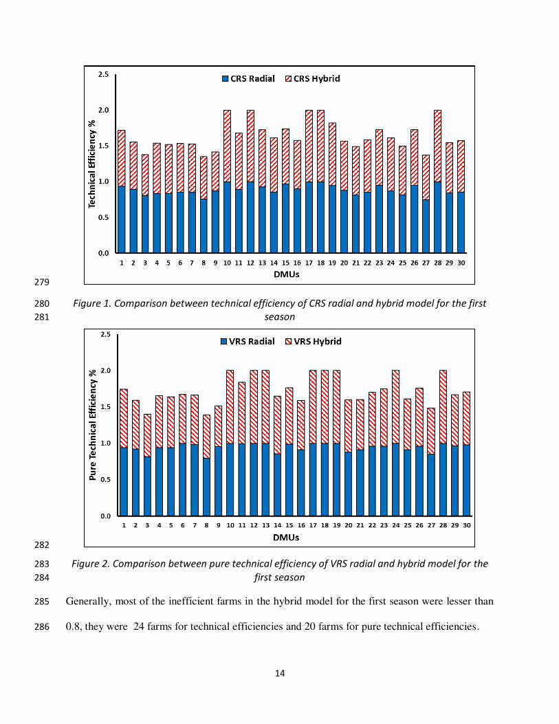
282

Figure 2. Comparison between pure technical efficiency of VRS radial and hybrid model for the 283

first season 284

Generally, most of the inefficient farms in the hybrid model for the first season were lesser than 285

0.8, they were 24 farms for technical efficiencies and 20 farms for pure technical efficiencies. 286

15

287

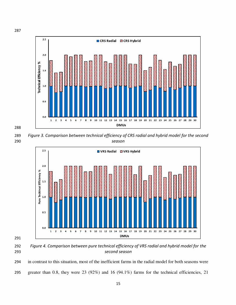
288

Figure 3. Comparison between technical efficiency of CRS radial and hybrid model for the second 289

season 290

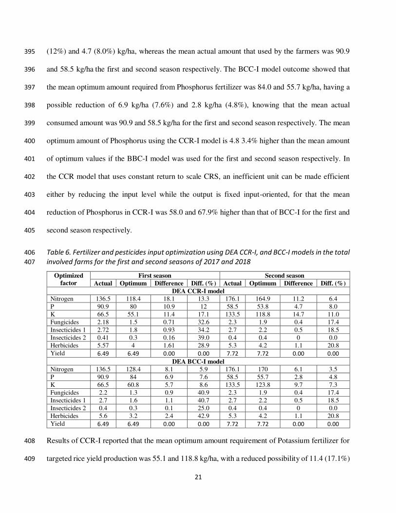
291

Figure 4. Comparison between pure technical efficiency of VRS radial and hybrid model for the 292

second season 293

in contrast to this situation, most of the inefficient farms in the radial model for both seasons were 294

greater than 0.8, they were 23 (92%) and 16 (94.1%) farms for the technical efficiencies, 21 295

16

(95.5%) and 13 (100%) farms for the pure technical efficiencies for first and second season 296

respectively. 297

Table 4 shows a comparison between the radial and hybrid models in technical efficiencies (CRS) 298

and pure technical efficiencies (VRS). Hybrid showed mean technical efficiency of 13 and 8% 299

lesser than that of the radial model, and mean pure technical efficiency of 16 and 7% lesser than 300

that of the radial model. The coefficient of variation CV of hybrid mode showed a high variation 301

in the efficiencies 17.3 and 14.9% for the technical efficiencies and 18.5 and 14.3% for the pure 302

technical efficiencies, and a very high standard deviation with 85.7 and 85.7% greater than that of 303

the radial model for technical efficiencies, 150 and 160% greater than that of the radial model for 304

pure technical efficiencies for first and second season respectively. This revealed that there was a 305

big difference between efficiencies in the hybrid and radial model, T-test showed that these 306

differences were highly significant P value < 0.001 for both efficiencies for the first season, and 307

P-value < 0.01 for both efficiencies for the second season. 308

Table 4. Comparison of mean technical and pure technical efficiency between the radial and 309

hybrid model for first and second season 2017-2018 310

Constant Return to Scale CRS Variable Return to Scale VRS

First Season Second Season First Season Second Season

Radial Hybrid Radial Hybrid Radial Hybrid Radial Hybrid

Mean 0.89±0.03 0.76±0.05 0.95±0.02 0.87±0.05 0.95±0.02 0.79±0.05 0.97±0.02 0.90±0.05

Max 1 1 1 1 1 1 1 1

Min 0.75 0.55 0.79 0.63 0.79 0.56 0.82 0.66

St. Dev. 0.07 0.13 0.07 0.13 0.06 0.15 0.05 0.13

CV % 8.14 17.33 6.83 14.92 6.17 18.54 4.89 14.25

P - value 0.00001*** 0.004*** 0.000002*** 0.004***

3.3. Comparing input use between efficient and inefficient farms based on CCR 311

In the DEA method using the CCR model, the efficient and inefficient farms remained constant in 312

both input and output-oriented methods, which means that the input resources and materials 313

remained the same for both models. The number of fertilizers and pesticide inputs and yield output 314

17

from different sources and output for efficient farmers and inefficient ones based on the CCR and 315

BCC models are given in Table 5. For the CCR model, the results revealed that efficient farms 316

used all of the physical inputs less than inefficient farmers. The outcome of CCR showed that the 317

mean amount of nitrogen used in the efficient farms was 130.8 and 165.7 kg/ha, while for the 318

inefficient farms was 137.6 and 184.1 kg/ha which is 5.2 and 11.1% more than the efficient farms 319

for the first and second season respectively. The mean amount used for Phosphorus fertilizer in 320

the efficient farms was 87.9 and 53.03 kg/ha, and that was 3.8 and 15.3% lesser than the mean 321

amount used Phosphorus by inefficient farms which were 91.5 and 62.6 kg/ha for the first and 322

second season respectively. 323

Table 5. Comparison of sources input and output yield ratios between efficient and inefficient 324

farms for various DEA models for the first and second seasons 2017 and 2018. 325

Details First season 2017 Second season 2018

Efficient

farms

Inefficient

farms

Difference

%

Efficient

farms

Inefficient

farms

Difference

%

CCR-I & CCR-O

Nitrogen input, kg/ha 130.80 137.6 5.18 165.68 184.05 11.09

Phosphorus input, kg/ha 87.94 91.45 3.99 53.03 62.63 18.10

Potassium input, kg/ha 64.11 66.92 4.38 115.68 147.06 27.13

Fungicides input, kg/ha 1.40 2.33 66.43 1.87 2.64 41.18

Insecticides input, l/ha 1.54 2.96 92.21 2.2 3.13 42.27

Insecticides input, kg/ha 0.26 0.44 69.23 0.38 0.47 23.68

Herbicides input, l/ha 4.00 5.88 47.00 4.62 5.81 25.76

Yield output, kg/ha 6.87 6.65 -3.20 6.91 7.37 6.66

BCC-I

Nitrogen input, kg/ha 148.90 132.68 -10.89 159.07 198.34 24.69

Phosphorus input, kg/ha 96.01 89.30 -6.99 51.33 67.8 32.09

Potassium input, kg/ha 69.87 65.41 -6.38 106.76 168.38 57.72

Fungicides input, kg/ha 1.67 2.33 39.52 2.08 2.61 25.48

Insecticides input, l/ha 1.89 2.98 57.67 2.39 3.18 33.05

Insecticides input, kg/ha 0.31 0.44 41.94 0.39 0.49 25.64

Herbicides input, l/ha 4.22 5.98 41.71 4.50 6.34 40.89

Yield output, kg/ha 7.30 6.49 -11.10 6.74 7.72 14.54

BCC-O

Nitrogen input, kg/ha 155.09 129.7 -16.37 160.98 193.35 20.11

Phosphorus input, kg/ha 98.56 88.07 -10.64 51.67 66.24 28.20

Potassium input, kg/ha 71.61 64.58 -9.82 109.14 161.26 47.76

Fungicides input, kg/ha 1.64 2.37 44.51 1.98 2.69 35.86

Insecticides input, l/ha 1.9 3.02 58.95 2.30 3.22 40.00

Insecticides input, kg/ha 0.32 0.44 37.50 0.39 0.48 23.08

Herbicides input, l/ha 4.33 6.02 39.03 4.48 6.23 39.06

Yield output, kg/ha 7.43 6.41 -13.73 6.79 7.59 11.78

18

Efficient farms consumed a mean amount of 64.1 and 115.7 kg of Potassium fertilizers, while 326

inefficient farms consumed 66.9 and 147.1 kg/ha and which is 4.4 and 27.1% more than that of 327

efficient farms, for the first and second season respectively. The mean amount used of fungicides 328

in the efficient farms was 1.4 and 1.9 l/ha, as for inefficient farms the mean used amount was 2.3 329

and 2.6 l/ha, showing 66.4 and 41.2% more amount used in the efficient ones for the first and 330

second season respectively. 331

Inefficient farms consumed 3 and 3.1 l/ha mean amount of liquid insecticides which is 92.2 and 332

42.3% more than the mean amount consumed by the efficient farms 1.54 and 2.2 l/h, for the first 333

and second seasons respectively. The mean amount of solid insecticides used by the inefficient 334

farms was 0.44 and 0.47 kg/ha, which is 69.2 and 23.7% higher than the mean amount used by the 335

efficient farms 0,26 and 0.38 kg/ha for the first and second seasons respectively. The efficient 336

farms consumed the mean amount of herbicides equal to 4.0 and 4.6 l/ha, while inefficient farms 337

consumed a mean amount of 5.9 and 5.8 l/ha, which is 47 and 25.8% higher that these efficient 338

ones, and that for the first and second season respectively. The mean amount of yield output for 339

inefficient farms is 6.6 and 7.3 tons/ha, which is 3.2% lesser and 6.7 higher than that of efficient 340

farms which had the mean amount of yield output of 6.87 and 6.91 ton/ha for the first and second 341

season respectively Table 5. 342

3.4. Comparison between efficient and inefficient farms based on BCC 343

In the DEA method using the BCC model, the efficient and inefficient farms do not remain 344

constant in both input and output-oriented methods, which means that the input resources and 345

materials are different for both models. The outcome of BCC-I showed that the mean amount of 346

nitrogen used in the efficient farms was 148.9 and 159.1 kg/ha, while for the inefficient farms was 347

132.7 and 198.3kg/ha for the first and second season respectively. The mean amount of Nitrogen 348

19

for inefficient farms in the first season is 10.9% lesser than the efficient farms, while it was 24.7% 349

more than the efficient farms for the second season. The mean amount used of Phosphorus fertilizer 350

in the efficient farms was 96.0 and 51.3 kg/ha, and the mean amount used of Phosphorus by 351

inefficient farms which were 89.3 and 67.8 kg/ha for the first and second season respectively. The 352

mean amount of Phosphorus for inefficient farms is 7% lesser and 32.1% higher than the efficient 353

farms, for the first and second season respectively. Efficient farms consumed a mean amount of 354

69.9 and 106.8 kg of Potassium fertilizers, while inefficient farms consumed 65.4 and 168.4 kg/ha 355

and which is 6.4% lesser and 57.7% more than efficient farms, for the first and second seasons 356

respectively. 357

The mean amount used of fungicides for efficient farms was 1.7 and 2.1 l/ha, as for inefficient 358

farms the mean used amount was 2.3 and 2.6 l/ha, showing 39.5 and 25.5% more amount used for 359

the efficient ones for the first and second season respectively. Inefficient farms consumed 3 and 360

3.2 l/ha mean amount of liquid insecticides which is 57.7 and 33.1% more than the mean amount 361

consumed by the efficient farms which were 1.9 and 2.4 l/h, for the first and second seasons 362

respectively. The mean amount of solid insecticides used by the inefficient farms was 0.44 and 363

0.49 kg/ha, which is 41.9 and 25.6% higher than the mean amount used by the efficient farms 0.31 364

and 0.39 kg/ha for the first and second seasons respectively. The efficient farms consumed a mean 365

amount of herbicides equal to 4.2 and 4.5 l/ha, while inefficient farms consumed a mean amount 366

of 6.0 and 6.3 l/ha, which is 41.7 and 40.9% higher than these efficient ones, for the first and 367

second season respectively. The mean amount of yield output for inefficient farms is 6.5 and 7.7 368

tons/ha, which is 11.1% lesser and 14.5% higher than that of efficient farms which had the mean 369

amount of yield output of 7.3 and 6.7 ton/ha for the first and second season respectively Table 5. 370

In this model BCC-I outcome, it was very clear that there is a big relation between fertilizer input 371

20

and yield output. For the first season, the Nitrogen, Phosphorus, and Potassium fertilizer of the 372

efficient farms were greater than that of inefficient farms, the same as the yield output which was 373

also greater in the efficient farms than that of inefficient farms. This revealed that the most 374

effective factor that determines the efficient farms and achieves and controls the efficiencies scores 375

3.4.1. Comparison of actual versus optimum sources inputs based on input-oriented 376

Table 6 shows the meant amount of actual used and optimum fertilizers and pesticides requirement 377

for rice production in wetland rice cultivation in Malaysia, based on the results of CCR-I and BCC-378

I input-oriented models. The quantity and percentage of fertilizers and pesticides saved concerning 379

the present use of the total fertilizers and pesticides used are illustrated. The outcome data of CCR-380

I showed that the optimum Nitrogen requirement amount was 136.5 and 176.1 kg/ha, with a 381

reduced possibility of 18.1 kg/ha (13.3%) and 11.2 kg/ha (6.4%), while the actual amount used 382

was 136.5 and 176.1 kg/ha for the first and second season respectively. But the outcome data of 383

BCC-I showed that the optimum requirement amount of Nitrogen was 128.4 and 170.0 kg/ha with 384

the possibility of a reduction of 8.1 kg/ha (5.9%) and 6.1 kg/ha (3.5%), with the mention that the 385

actual amount of Nitrogen used was 136.5 and 176.1 kg/ha for the first and second season 386

respectively. These data showed that the optimum values in BCC-I are 8.4 and 3.1% more than 387

the optimum amount in the CCR-I model for the first and second season respectively. The 388

reduction amount that is possible in CCR-I without any negative effects on the yield output is 389

123.5 and 83.6% higher than that of the BCC-I model for the first and second season respectively, 390

and this showed the strength of CCR-I over BCC-I in terms of optimizing the input amount and 391

keeping the amount of input constant. 392

The CCR-I outcome revealed that the mean optimum Phosphorus requirement amount for rice 393

production in the study area was found to be 80 and 53.8 kg/ha, with a reduced possibility of 10.9 394

21

(12%) and 4.7 (8.0%) kg/ha, whereas the mean actual amount that used by the farmers was 90.9 395

and 58.5 kg/ha the first and second season respectively. The BCC-I model outcome showed that 396

the mean optimum amount required from Phosphorus fertilizer was 84.0 and 55.7 kg/ha, having a 397

possible reduction of 6.9 kg/ha (7.6%) and 2.8 kg/ha (4.8%), knowing that the mean actual 398

consumed amount was 90.9 and 58.5 kg/ha for the first and second season respectively. The mean 399

optimum amount of Phosphorus using the CCR-I model is 4.8 3.4% higher than the mean amount 400

of optimum values if the BBC-I model was used for the first and second season respectively. In 401

the CCR model that uses constant return to scale CRS, an inefficient unit can be made efficient 402

either by reducing the input level while the output is fixed input-oriented, for that the mean 403

reduction of Phosphorus in CCR-I was 58.0 and 67.9% higher than that of BCC-I for the first and 404

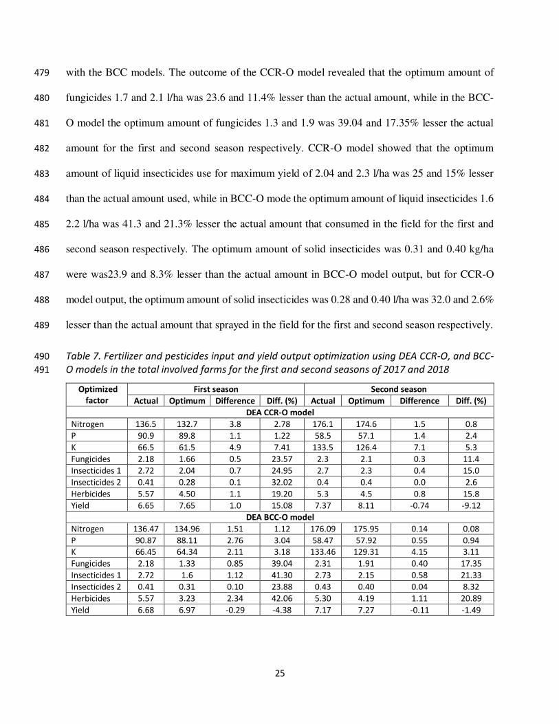
second season respectively. 405

Table 6. Fertilizer and pesticides input optimization using DEA CCR-I, and BCC-I models in the total 406

involved farms for the first and second seasons of 2017 and 2018 407

Optimized

factor

First season Second season

Actual Optimum Difference Diff. (%) Actual Optimum Difference Diff. (%)

DEA CCR-I model

Nitrogen 136.5 118.4 18.1 13.3 176.1 164.9 11.2 6.4

P 90.9 80 10.9 12 58.5 53.8 4.7 8.0

K 66.5 55.1 11.4 17.1 133.5 118.8 14.7 11.0

Fungicides 2.18 1.5 0.71 32.6 2.3 1.9 0.4 17.4

Insecticides 1 2.72 1.8 0.93 34.2 2.7 2.2 0.5 18.5

Insecticides 2 0.41 0.3 0.16 39.0 0.4 0.4 0 0.0

Herbicides 5.57 4 1.61 28.9 5.3 4.2 1.1 20.8

Yield 6.49 6.49 0.00 0.00 7.72 7.72 0.00 0.00

DEA BCC-I model

Nitrogen 136.5 128.4 8.1 5.9 176.1 170 6.1 3.5

P 90.9 84 6.9 7.6 58.5 55.7 2.8 4.8

K 66.5 60.8 5.7 8.6 133.5 123.8 9.7 7.3

Fungicides 2.2 1.3 0.9 40.9 2.3 1.9 0.4 17.4

Insecticides 1 2.7 1.6 1.1 40.7 2.7 2.2 0.5 18.5

Insecticides 2 0.4 0.3 0.1 25.0 0.4 0.4 0 0.0

Herbicides 5.6 3.2 2.4 42.9 5.3 4.2 1.1 20.8

Yield 6.49 6.49 0.00 0.00 7.72 7.72 0.00 0.00

Results of CCR-I reported that the mean optimum amount requirement of Potassium fertilizer for 408

targeted rice yield production was 55.1 and 118.8 kg/ha, with a reduced possibility of 11.4 (17.1%) 409

22

and 14.7 (11.0%) for the first and second season respectively, while the results of BCC-I showed 410

that the meant optimum amount of Potassium required for rice production was 60.8 and 123.8 411

kg/ha, and the reduction could be 5.7 kg/ha (8.6%) and 9.7 kg/ha (7.3%), while the mean actual 412

amount used by the farmers in their farms was 66.5 and 133.5 kg/ha for the first and second season 413

respectively. The mean optimum amount of Potassium used in BCC-I with producing the same 414

yield as in CCR-I was 10.3 and 4.2% lesser than that of CCR-I for the first and second season 415

respectively. In CCR-I, the mean possible reduction of Potassium with producing the same yield 416

was 100 and 51.5% higher than that of the BCC-I model for the first and second season 417

respectively. 418

Using the CCR-I model showed that the mean optimum amount of fungicides required for rice 419

production was 1.5 and 1.9 l/ha, and the possible reduced amount without affecting the output 420

yield was 0.71 l/ha (32.6%) and 0.4 l/ha (17.4%), whereas the mean actual amount that used by 421

the farmers was 2.18 and 2.2 l/ha for the first and second season respectively. But for the BCC-I 422

model, the mean optimum amount of fungicides required to produce the same yield as in CCR-I 423

was 1.3 and 1.9 l/ha, and the reduction could be 0.9 l/ha (40.9%) and 0.4 l/ha (17.4%), mentioning 424

that the mean actual amount of fungicides sprayed by the farmers in their farms was 2.2.and 2.3 425

l/ha for the first and second season respectively. The data showed that the mean optimum values 426

of sprayed fungicides in CCR-I are 12.1 and 0.8% lesser than the optimum amount in the BCC-I 427

model for the first and second season respectively. The mean reduction of fungicides in CCR-I 428

was 21.1 and 3.9% higher than that of BCC-I for the first and second season respectively. 429

The mean optimum amount of liquid insecticides that should be used to produce the rice Known 430

yield using DEA CCR-I, was 1.8 and 2.2 l/ha, with the possible reduction of 0.93 l/ha (32.6%) and 431

0.5 l/ha (18.5%), while the mean actual amount sprayed by the farmers in their fields was 2.7 and 432

23

2.7 for the first and second season respectively. Using techniques of the BCC-I model showed that 433

the mean optimum amount of liquid insecticides was 1.6 and 2.2 l/ha, and could be reduced by the 434

mean amount of 1.1 l/ha (40.7%) and 0.5 l/ha (18.5%), whereas the mean amount of actual liquid 435

insecticides that sprayed in the fields was 2.7 and 2.7 for the first and second season respectively. 436

The mean amount of liquid insecticides required to produce the same yield and by using the 437

technique of the BCC-I model is 17.4 and 0.52% lesser than that of the CCR-I model for the first 438

and second seasons respectively. The CCR-I showed that the mean amount of possible reduction 439

of liquid insecticides and producing the same yield is 60 and 6.7% higher than that of BCC-I, for 440

the first and second seasons respectively. The mean optimum amount of herbicides was 4 and 4.2 441

l/ha in the CCR-I model, and 3.2 and 4.2 in the BCC-I model, which is lesser than the first one by 442

-18.1 and 0.5%, while the CCR-I model output had a mean reduction amount that was 32.9 and 443

2.1% higher than that of BCC-I model output. The yield for both models CCR-I and BCC-I 444

remained constant and there was no difference due to the orientation of the models as both of them 445

were input-oriented so the yield was not affected and not changed. 446

3.4.2. Comparison of actual and optimum inputs and output based on output-oriented 447

Some researchers reported that In the CCR model that using constant return to scale CRS, an 448

inefficient unit can be made efficient either by reducing the input level while the output is fixed 449

input-oriented or by increasing the output level while the input is fixed (output-oriented), this is 450

true in the first part of it and truly false in last part. It is true that in constant return to scale, in the 451

input-oriented CCR model, the movement just happens always in the input amount and the output 452

remains constant, but for CRS constant return to scale with output-oriented, there is no 453

proportionate movement but there is the slack movement which means that there is a change 454

happen to the input although it is very small it still happens. 455

24

The outcome of the DEA CCR-O model showed that the optimum amount of Nitrogen fertilizer 456

to produce the maximum yield output was 132.7 and 174.6 kg/ha which is 2.8% (3.8 k/ha) and 457

0.8% (1.5 kg/ha) lesser than the used amount which was 136.5 and 176.1 kg/ha, while for DEA 458

BCC-O model, the mean optimum amount of Nitrogen fertilizers was 134.96 and 175.95 kg/ha, 459

and that is 1.12% (1.51 kg/ha) and 0.08% (0.14 kg/ha) than the mean actual amount that 460

broadcasted in the fields for the first and second season respectively. This revealed that, when the 461

orientation of the DEA CCR and BCC model is output-oriented, there is a change that happens to 462

the inputs but it is always very small changes. The mean optimum amount of Nitrogen input in 463

CCR-O is 1.7 and 0.77% lesser than that of BCC-O, while the possible reduction of Nitrogen 464

amount to achieve the maximum potential yield output in BCC-O is 60.26 and 90.67% lesser than 465

that of CCR-O model for the first and second season respectively. The mean optimum amount of 466

Phosphorus needed to produce the maximum yield in the BCC-O model is 88.11 and 57.92 kg/ha 467

and that is 1.9% lesser and 1.4% more than the mean optimum amount of Phosphorus when using 468

the CCR-O model which was 89.8 and 57.1 kg/ha, with mentioning that the possible reduction of 469

Phosphorus to achieve the maximum yield was 60.14% lesser and 154.6% higher than BCC-O 470

model when using CCR-O model for the first and second season respectively. The optimum 471

amount of Potassium required for maximum yield production was 61.5 and 126.4 kg/ha in the 472

CCR-O model, 64.3 and 129.3 kg/ha in the BCC-O model, and this last one is 4.6 and 2.3% higher 473

than the first one, and the mean reduction amount of Phosphorus that could be done was 132.2 and 474

71.1% higher in CCR-O model than that of BCC-O model for the first and second season 475

respectively. 476

The CCR models are the most rigorous ones, because they compare the respective DMU with all 477

linear combinations of the other DMUs, and not only with their convex combinations as is the case 478

25

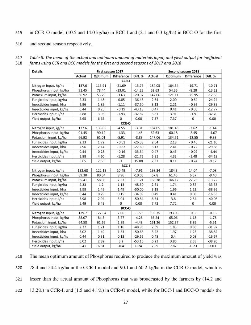
with the BCC models. The outcome of the CCR-O model revealed that the optimum amount of 479

fungicides 1.7 and 2.1 l/ha was 23.6 and 11.4% lesser than the actual amount, while in the BCC-480

O model the optimum amount of fungicides 1.3 and 1.9 was 39.04 and 17.35% lesser the actual 481

amount for the first and second season respectively. CCR-O model showed that the optimum 482

amount of liquid insecticides use for maximum yield of 2.04 and 2.3 l/ha was 25 and 15% lesser 483

than the actual amount used, while in BCC-O mode the optimum amount of liquid insecticides 1.6 484

2.2 l/ha was 41.3 and 21.3% lesser the actual amount that consumed in the field for the first and 485

second season respectively. The optimum amount of solid insecticides was 0.31 and 0.40 kg/ha 486

were was23.9 and 8.3% lesser than the actual amount in BCC-O model output, but for CCR-O 487

model output, the optimum amount of solid insecticides was 0.28 and 0.40 l/ha was 32.0 and 2.6% 488

lesser than the actual amount that sprayed in the field for the first and second season respectively. 489

Table 7. Fertilizer and pesticides input and yield output optimization using DEA CCR-O, and BCC-490

O models in the total involved farms for the first and second seasons of 2017 and 2018 491

Optimized

factor

First season Second season

Actual Optimum Difference Diff. (%) Actual Optimum Difference Diff. (%)

DEA CCR-O model

Nitrogen 136.5 132.7 3.8 2.78 176.1 174.6 1.5 0.8

P 90.9 89.8 1.1 1.22 58.5 57.1 1.4 2.4

K 66.5 61.5 4.9 7.41 133.5 126.4 7.1 5.3

Fungicides 2.18 1.66 0.5 23.57 2.3 2.1 0.3 11.4

Insecticides 1 2.72 2.04 0.7 24.95 2.7 2.3 0.4 15.0

Insecticides 2 0.41 0.28 0.1 32.02 0.4 0.4 0.0 2.6

Herbicides 5.57 4.50 1.1 19.20 5.3 4.5 0.8 15.8

Yield 6.65 7.65 1.0 15.08 7.37 8.11 -0.74 -9.12

DEA BCC-O model

Nitrogen 136.47 134.96 1.51 1.12 176.09 175.95 0.14 0.08

P 90.87 88.11 2.76 3.04 58.47 57.92 0.55 0.94

K 66.45 64.34 2.11 3.18 133.46 129.31 4.15 3.11

Fungicides 2.18 1.33 0.85 39.04 2.31 1.91 0.40 17.35

Insecticides 1 2.72 1.6 1.12 41.30 2.73 2.15 0.58 21.33

Insecticides 2 0.41 0.31 0.10 23.88 0.43 0.40 0.04 8.32

Herbicides 5.57 3.23 2.34 42.06 5.30 4.19 1.11 20.89

Yield 6.68 6.97 -0.29 -4.38 7.17 7.27 -0.11 -1.49

26

CCR-O model output revealed that the optimum amount of herbicides 4.5 and 4.5 l/ha was 19.2 492

and 15.8% lesser than the actual amount, while in the BCC-O model, the optimum amount of 493

herbicides 3.23 and 4.19. l/ha was 42.1 and 20.9% lesser than the actual amount of herbicides that 494

were used in the farms for the first and second season respectively. The values differ in BCC (VRS 495

DEA), from what was found from the evaluations in CCR (CRS DEA). 496

3.5. Resources saved from different sources inputs in inefficient farms 497

Table 5 shows the optimum resource requirement and saving materials for rice production in 498

wetlands based on the results of CCR and BCC models in the inefficient farms for the first and 499

second seasons of 2017 and 2018. As mentioned above the efficient farms were 5 and 13 in CCR 500

input and output-oriented, 7 and 17 for the BCC-I model and they were 8 and 16 efficient farms 501

for the BCC-O model for the first and second season respectively. The inefficient farms were 25 502

and 17 farms in CCR for both dimensions input and output, 23 and 13 inefficient farms in the 503

BCC-I model and there were 22 and 14 inefficient farms in the BCC-O model for the first and 504

second seasons respectively. 505

As shown in Table 8, the mean optimum Nitrogen input used by farmers in cultivating one-hectare 506

farmland in inefficient farms, was 115.9 and 164.34 kg/ha in the CCR-I model, 133.1 and 181.4 507

kg/ha in the CCR-O model, 122.2 and 184.3 kg/ha in BCC-I model, and was 127.6 and 193.1 in 508

BCC-O model, while the actual amount was (137.6 and 184.1 kg/ha) in CCR-I and CCR-O models, 509

(132.7 and 198.34 kg/ha) in BCC-I model and it was (129.7 and 193.35 kg/ha) IN BCC-O model 510

for the first and second season respectively. The mean optimum Nitrogen input was lesser than the 511

mean observed Nitrogen expenditure by 15.8 and 10.71% in the CCR-I model, 3.31 and 1.44% in 512

the CCR-O model, 7.91 and 7.08% in the BCC-I model, and lastly, 1.6 and 0.2% in BCC-O, 513

revealed that excess usage of up to (21.7 and 19.7 kg/ha) in CCR-I model and (4.6 and 2.6 kg/ha) 514

27

in CCR-O model, (10.5 and 14.0 kg/ha) in BCC-I and (2.1 and 0.3 kg/ha) in BCC-O for the first 515

and second season respectively. 516

Table 8. The mean of the actual and optimum amount of materials input, and yield output for inefficient 517

farms using CCR and BCC models for the first and second seasons of 2017 and 2018 518

Details First season 2017 Second season 2018

Actual Optimum Difference Diff. % Actual Optimum Difference Diff. %

CCR-I

Nitrogen input, kg/ha 137.6 115.91 -21.69 -15.76 184.05 164.34 -19.71 -10.71

Phosphorus input, kg/ha 91.45 78.44 -13.01 -14.23 62.63 54.35 -8.28 -13.22

Potassium input, kg/ha 66.92 53.29 -3.63 -20.37 147.06 121.11 -25.95 -17.65

Fungicides input, kg/ha 2.33 1.48 -0.85 -36.48 2.64 2.00 - 0.64 -24.24

Insecticides input, l/ha 2.96 1.85 -1.11 -37.50 3.13 2.21 - 0.92 -29.39

Insecticides input, kg/ha 0.44 0.25 - 0.19 -43.18 0.47 0.41 - 0.06 -12.77

Herbicides input, l/ha 5.88 3.95 -1.93 -32.82 5.81 3.91 -1.9 -32.70

Yield output, kg/ha 6.65 6.65 0 0.00 7.37 7.37 0 0.00

CCR-O

Nitrogen input, kg/ha 137.6 133.05 -4.55 -3.31 184.05 181.43 -2.62 -1.44

Phosphorus input, kg/ha 91.45 90.12 -1.33 -1.45 62.63 60.18 -2.45 - 4.07

Potassium input, kg/ha 66.92 61.01 -5.91 -8.83 147.06 134.51 -12.55 -9.33

Fungicides input, kg/ha 2.33 1.72 - 0.61 -26.38 2.64 2.18 - 0.46 -21.10

Insecticides input, l/ha 2.96 2.14 - 0.82 -27.60 3.13 2.41 - 0.72 -29.88

Insecticides input, kg/ha 0.44 0.28 - 0.16 -35.54 0.47 0.45 - 0.02 - 4.44

Herbicides input, l/ha 5.88 4.60 -1.28 -21.75 5.81 4.33 -1.48 -34.18

Yield output, kg/ha 6.65 7.65 -1 15.08 7.37 8.11 - 0.74 -9.12

BCC-I

Nitrogen input, kg/ha 132.68 122.19 10.49 -7.91 198.34 184.3 14.04 -7.08

Phosphorus input, kg/ha 89.30 80.34 8.96 -10.03 67.8 61.43 6.37 -9.40

Potassium input, kg/ha 65.41 58.08 7.33 -11.21 168.38 146.12 22.26 -13.22

Fungicides input, kg/ha 2.33 1.2 1.13 -48.50 2.61 1.74 0.87 -33.33

Insecticides input, l/ha 2.98 1.49 1.49 -50.00 3.18 1.96 1.22 -38.36

Insecticides input, kg/ha 0.44 0.29 0.15 -34.09 0.49 0.41 0.08 -16.33

Herbicides input, l/ha 5.98 2.94 3.04 -50.84 6.34 3.8 2.54 -40.06

Yield output, kg/ha 6.49 6.49 0 0.00 7.72 7.72 0 0.00

BCC-O

Nitrogen input, kg/ha 129.7 127.64 2.06 -1.59 193.35 193.05 0.3 -0.16

Phosphorus input, kg/ha 88.07 84.3 3.77 -4.28 66.24 65.06 1.18 -1.78

Potassium input, kg/ha 64.58 61.69 2.89 -4.48 161.26 152.37 8.89 -5.51

Fungicides input, kg/ha 2.37 1.21 1.16 -48.95 2.69 1.83 0.86 -31.97

Insecticides input, l/ha 3.02 1.49 1.53 -50.66 3.22 1.97 1.25 -38.82

Insecticides input, kg/ha 0.44 0.31 0.13 -29.55 0.48 0.4 0.08 -16.67

Herbicides input, l/ha 6.02 2.82 3.2 -53.16 6.23 3.85 2.38 -38.20

Yield output, kg/ha 6.41 6.81 -0.4 6.24 7.59 7.82 -0.23 3.03

The mean optimum amount of Phosphorus required to produce the maximum amount of yield was 519

78.4 and 54.4 kg/ha in the CCR-I model and 90.1 and 60.2 kg/ha in the CCR-O model, which is 520

lesser than the actual amount of Phosphorus that was broadcasted by the farmers by (14.2 and 521

13.2%) in CCR-I, and (1.5 and 4.1%) in CCR-O model, while for BCC-I and BCC-O models the 522

28

optimum amount was (80.3 and 61.4 kg/ha) and (84.3 and 65.1 kg/ha) and that is (10.0 and 9.4%) 523

and (4.3 and 1.8%) lesser than the used amount which revealed that excess usage of up to (9 and 524

6.4 kg/ha) in BCC-I and (3.4 and 1.2 kg/ha) in BCC-O for the first and second season respectively. 525

The mean optimum amount of Potassium required for maximum yield production in CCR-I, CCR-526

O, BCC-I, and BCC-O models was lesser than the actual amount that consumed in the farms by 527

[20.4% (53.3 vs. 66.9 kg/ha), and 17.7% (121.1 vs. 147.1)], [8.8% (61.0 vs. 66.9 kg/ha), and 9.3% 528

(134.5 vs. 147.1)], [11.2% (58.1 vs. 65.4 kg/ha), and 13.2% (146.1 vs. 168.4 kg/ha)] and lastly 529

[4.5% (61.7 vs. 64.6 kg/ha), and 5.5% (152.4 vs. 161.3 kg/ha)] for the first and second season 530

respectively (Table 8). The study revealed that there was excess amount usage of Potassium up to 531

(13.6 and 25.95 kg/ha), (5.9 and 12.6 kg/ha), (7.3 and 22.3 kg/ha), and (2.9 and 8.9 kg/ha) in CCR-532

I model, CCR-O model, BCC-I model, and BCC-O model for the first and second season 533

respectively. The excess amount of inputs is always higher when we used CCR than that of BCC 534

in the same direction meaning the input-oriented and the output-oriented but is that advantage or 535

disadvantage for this model CCR (Table 8). 536

The result showed that the mean optimum amount of fungicides was (1.5 and 2.0 l/ha) in the CCR-537

I model, (1.7 and 2.2 l/ha) in the CCR-O model, (1.2 and 1.7 l/ha) in BCC-I model, and (1,2 and 538

1.8 l/ha) in BCC-O model, while the mean actual amount of fungicides sprayed in the inefficient 539

farms were (2.3 and 2.6 l/ha) in both CCR models, (2.3 and 2.6 l/ha) in BCC-I model, and (2.4 and 540

2.7 l/ha) in BCC-O outcome, the excess expenditure of fungicides was (0.9 l/ha (35.5%) and 0.6 541

l/ha (24.2%)) in CCR-I model outcome, (0.6 l/ha (26.4%) and 0.5 l/ha (21.1%) in CCR-O model 542

outcome, (1.1 l/ha (48.5%) and 0.9 l/ha (33.3%) in BCC-I model outcome, and (1.2 l/ha (49%) and 543

0.9 l/ha (32%) in BCC-O model outcome for the first and second season respectively. The DEA 544

models result cleared that the mean optimum amount of liquid insecticides was (1.9 and 2.2 l/ha) 545

29

in the CCR-I model outcome, (2.14 and 2.4 l/ha) in the CCR-O model outcome, (1.5 and 2.0 l/ha) 546

in BCC-I model outcome, and (1.5 and 1.5 l/ha) in BCC-O model outcome, while the mean actual 547

amount of liquid insecticides sprayed in the inefficient farms was (3.0 and 3.1 l/ha) in both CCR 548

models outcomes, (3 and 3.2 /ha) in BCC-I model outcome, and (3.0 and 3.2 l/ha) in BCC-O model 549

outcome, the mean excess expended amount of liquid insecticides was (1.1 l/ha (37.5%) and 0.9 550

l/ha (29.4%)) in CCR-I model outcome, (0.8 l/ha (27.6%) and 0.7 l/ha (29.9%) in CCR-O model 551

outcome, (1.5 l/ha (50.0%) and 1.2 l/ha (38.4%) in BCC-I model outcome, and (1.5 l/ha (50.7%) 552

and 1.3 l/ha (38.8%) in BCC-O model outcome for the first and second season respectively. The 553

DEA models summary result explained that the mean optimum amount of solid insecticides was 554

(0.25 and 0.41 l/ha) in the CCR-I model outcome, (0.28 and 0.45 l/ha) in the CCR-O model 555

outcome, (0.29 and 0.08 l/ha) in BCC-I model outcome, and (0.31 and 0.08 l/ha) in BCC-O model 556

outcome, while the mean actual amount of solid insecticides sprayed in the inefficient farms was 557

(0.44 and 0.47 l/ha) in both CCR models outcomes, (0.44 and 0.49 /ha) in BCC-I model outcome, 558

and (0.44 and 0.48 l/ha) in BCC-O model outcome, the mean excess expended amount of solid 559

insecticides was (0.19 l/ha 43.2%) and 0.06 l/ha (12.8%)) in CCR-I model outcome, (0.16 l/ha 560

(35.5%) and 0.02 l/ha (4.4%) in CCR-O model outcome, (0.15 l/ha (34.1%) and 0.08 l/ha (16.3%) 561

in BCC-I model outcome, and (0.13 l/ha (29.6%) and 0.08 l/ha (16.7%) in BCC-O model outcome 562

for the first and second season respectively (Table 8). 563

The mean optimum amount of herbicides after running CCR and BCC models for the two 564

directions were (4.0 and 3.9 l/ha) in the CCR-I model outcome, (4.6 and 4.3 l/ha) in the CCR-O 565

model outcome, (2.9 and 2.5 l/ha) in BCC-I model outcome, and (2.8 and 3.9 l/ha) in BCC-O 566

model outcome, while the mean actual amount of herbicides consumed in the inefficient farms was 567

(5.9 and 5.8 l/ha) in both CCR models outcomes, (6.0 and 6.3 l/ha) in BCC-I model outcome, and 568

30

(6.0 and 6.2 l/ha) in BCC-O model outcome, the mean excess expenditure of herbicides was (1.9 569

l/ha (32.8%) and 1.9 l/ha (32.7%)) in CCR-I model outcome, (1.3 l/ha (21.8%) and 1.5 l/ha (34.2%) 570

in CCR-O model outcome, (3.0 l/ha (50.8%) and 2.5 l/ha (40.1%) in BCC-I model outcome, and 571

(3.2 l/ha (53.2%) and 2.4 l/ha (38.2%) in BCC-O model outcome for the first and second season 572

respectively. The result of herbicides optimization showed a higher amount of excess usage and a 573

very high percentage of materials that could be saved, especially that the herbicides consumed in 574

a high amount for one hectare, the farmers could reduce that if they follow the instructions of Rice 575

Check by burning the rice straws immediately after harvesting which prevent weedy rice and other 576

weeds from re-growing again. Following the standard of Rice Check and Good Agricultural 577

Practice GAP could achieve a very good result in terms of reducing input resources and increasing 578

rice yield output (Table 8). 579

3.6. Analyzing the optimization of inputs based on SBM models 580

SBM-I-C model reduced the actual amount of Nitrogen by 8.5 and 11 kg/ha which is 53.1 and 581

1.8% lesser than that of CCR-I and reduced the actual amount of Phosphorus by 6.6 and 6.6 kg/ha 582

which is 39.2% lesser and 41.5% more than that of CCR-I, reduced the actual amount of Potassium 583

by 3.7 and 11.4 kg/ha and that is 67.4 and 22.5% lesser than that of CCR-I for first and second 584

season respectively. Also, the SBM-I-C model reduced fungicides by 1.0 and 0.5 l/ha, liquid 585

insecticides by 1.4 and 0.7 l/ha, and reduced herbicides by 3 and 1.7 l/ha and which is more than 586

that of CCR-I by 45.1 and 39.7%, 47.4 and 30.2%, and 83.5 and 56.3%, while it reduced solid 587

insecticides by 0.1 and 0.03 l/ha which is lesser than that of CCR-I BY 37.7 and 16.1%for first 588

and second season respectively (Table 9). SBM-I-V reduced Nitrogen by 2.2% more and 41.9% 589

lesser, Phosphorus by 0.6 and 39.7% more, Potassium 2% more, and 18.4% lesser than that of 590

BCC-I for the first and second season respectively. This model reduced fungicides by 2.5 and 591

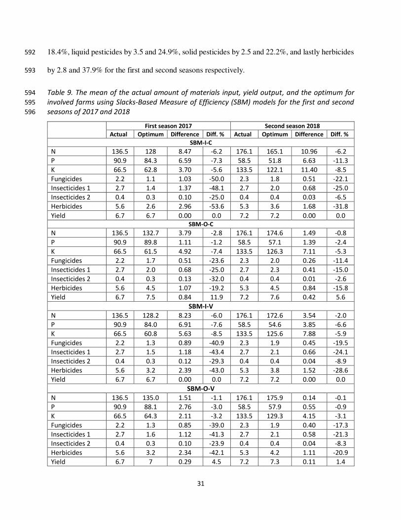
31

18.4%, liquid pesticides by 3.5 and 24.9%, solid pesticides by 2.5 and 22.2%, and lastly herbicides 592

by 2.8 and 37.9% for the first and second seasons respectively. 593

Table 9. The mean of the actual amount of materials input, yield output, and the optimum for 594

involved farms using Slacks-Based Measure of Efficiency (SBM) models for the first and second 595

seasons of 2017 and 2018 596

First season 2017 Second season 2018

Actual Optimum Difference Diff. % Actual Optimum Difference Diff. %

SBM-I-C

N 136.5 128 8.47 -6.2 176.1 165.1 10.96 -6.2

P 90.9 84.3 6.59 -7.3 58.5 51.8 6.63 -11.3

K 66.5 62.8 3.70 -5.6 133.5 122.1 11.40 -8.5

Fungicides 2.2 1.1 1.03 -50.0 2.3 1.8 0.51 -22.1

Insecticides 1 2.7 1.4 1.37 -48.1 2.7 2.0 0.68 -25.0

Insecticides 2 0.4 0.3 0.10 -25.0 0.4 0.4 0.03 -6.5

Herbicides 5.6 2.6 2.96 -53.6 5.3 3.6 1.68 -31.8

Yield 6.7 6.7 0.00 0.0 7.2 7.2 0.00 0.0

SBM-O-C

N 136.5 132.7 3.79 -2.8 176.1 174.6 1.49 -0.8

P 90.9 89.8 1.11 -1.2 58.5 57.1 1.39 -2.4

K 66.5 61.5 4.92 -7.4 133.5 126.3 7.11 -5.3

Fungicides 2.2 1.7 0.51 -23.6 2.3 2.0 0.26 -11.4

Insecticides 1 2.7 2.0 0.68 -25.0 2.7 2.3 0.41 -15.0

Insecticides 2 0.4 0.3 0.13 -32.0 0.4 0.4 0.01 -2.6

Herbicides 5.6 4.5 1.07 -19.2 5.3 4.5 0.84 -15.8

Yield 6.7 7.5 0.84 11.9 7.2 7.6 0.42 5.6

SBM-I-V

N 136.5 128.2 8.23 -6.0 176.1 172.6 3.54 -2.0

P 90.9 84.0 6.91 -7.6 58.5 54.6 3.85 -6.6

K 66.5 60.8 5.63 -8.5 133.5 125.6 7.88 -5.9

Fungicides 2.2 1.3 0.89 -40.9 2.3 1.9 0.45 -19.5

Insecticides 1 2.7 1.5 1.18 -43.4 2.7 2.1 0.66 -24.1

Insecticides 2 0.4 0.3 0.12 -29.3 0.4 0.4 0.04 -8.9

Herbicides 5.6 3.2 2.39 -43.0 5.3 3.8 1.52 -28.6

Yield 6.7 6.7 0.00 0.0 7.2 7.2 0.00 0.0

SBM-O-V

N 136.5 135.0 1.51 -1.1 176.1 175.9 0.14 -0.1

P 90.9 88.1 2.76 -3.0 58.5 57.9 0.55 -0.9

K 66.5 64.3 2.11 -3.2 133.5 129.3 4.15 -3.1

Fungicides 2.2 1.3 0.85 -39.0 2.3 1.9 0.40 -17.3

Insecticides 1 2.7 1.6 1.12 -41.3 2.7 2.1 0.58 -21.3

Insecticides 2 0.4 0.3 0.10 -23.9 0.4 0.4 0.04 -8.3

Herbicides 5.6 3.2 2.34 -42.1 5.3 4.2 1.11 -20.9

Yield 6.7 7 0.29 4.5 7.2 7.3 0.11 1.4

32

SBM-O-C reduced the actual amount of Nitrogen by 3.8 and 1.5 kg/ha, Phosphorus by 1.1 and 1.4 597

kg/ha, Potassium by 4.9 and 7.1 kg, fungicides by 0.5 and 0.3 l/ha, liquid insecticides by 0.7 and 598

0.4 l/ha, solid insecticides by 0.13 and 0.1 kg/ha and herbicides by 1.1 and 0.8 l/ha for first and 599

second season respectively. These reductions are similar to that of the CCR-O model. SBM-O-V 600

reduced the actual amount of Nitrogen by 1.5 and 0.14 kg/ha, Phosphorus by 2.8 and 0.5 kg/ha, 601

Potassium by 2.1 and 4.2 kg/ha, Fungicides by 0.8 and 0.4 l/ha, liquid insecticides by 1.1 and 0.6 602

l/ha, solid insecticides by 0.1 and 0.04 kg/ha, and herbicides by 2.3 and 1.1 l/ha for first and second 603

season respectively. This model gave a similar result to BCC-O except for Nitrogen as it reduced 604

the actual amount by 0.04 and 0.14% for the first and second seasons respectively. 605

All the optimization models showed that there were access amounts of input consumptions 606

fertilizers and pesticides with different percentages according to every model, these models 607

showed that the amount of input could be reduced without affecting the rice grain output yield. 608

The result showed that the CCR-I had the highest reduction of the actual amount of input used and 609

gave the minimum amount for the optimum inputs. This revealed that CCR models are the most 610

stringent model, because this model compares the related DMU to all linear combinations of other 611

DMUs, and not just with convex groups as is the case with BCC models. The CCR model assumes 612

a radial expansion and reduction of all observed DMUs while the BCC model only accepts the 613

convex combinations of the DMUs as the production possibility set. 614

Analysis of variance One-way ANOVA showed that there were no significant between the 615

optimum amount of Nitrogen for the four models P = 0.46 and 0.74, for Phosphorus P = 0.74 and 616

0.75, and for Potassium P = 0.18 and 0.96 for the first and the second season. Grouping information 617

using the Dunnett method, Fisher LSD method, and the Tukey Method and 95% Confidence 618

showed that there were no significant differences between the means of optimum Nitrogen, 619

33

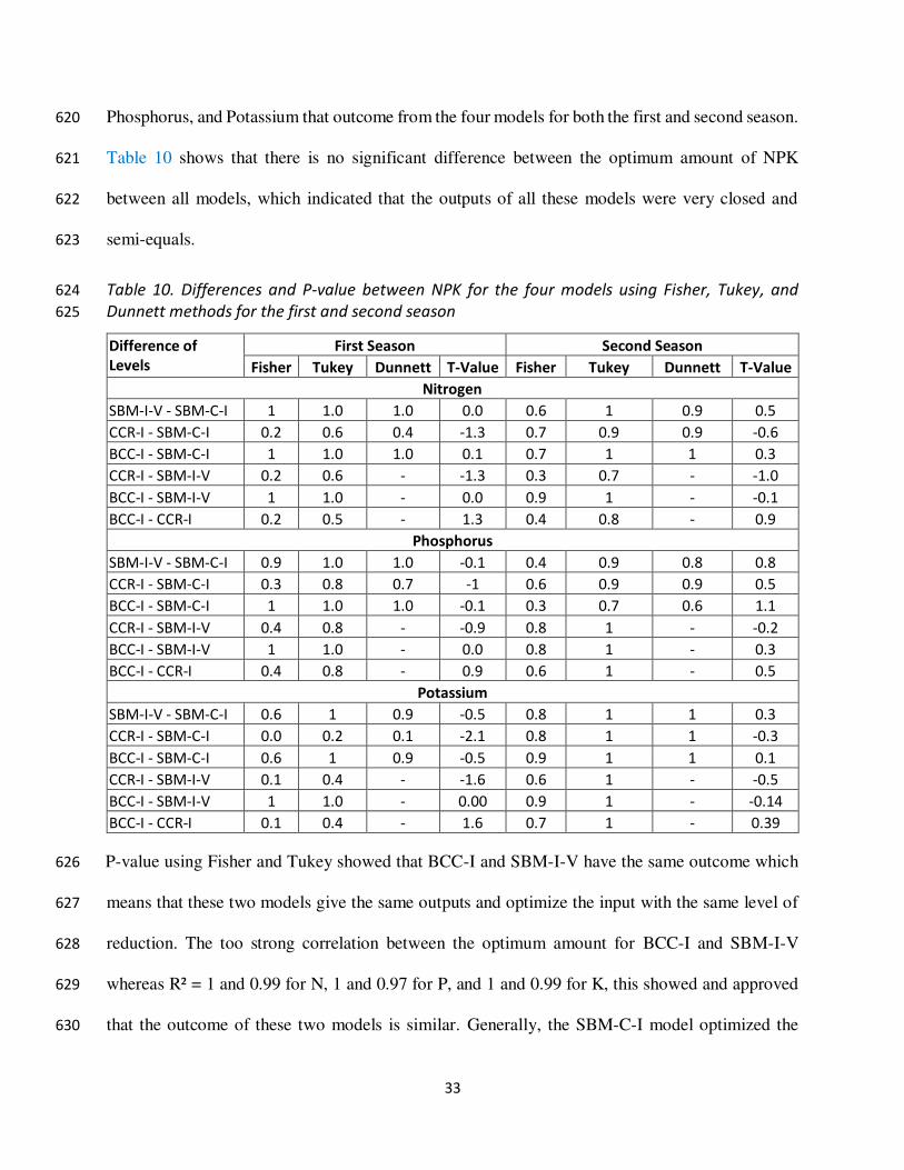
Phosphorus, and Potassium that outcome from the four models for both the first and second season. 620

Table 10 shows that there is no significant difference between the optimum amount of NPK 621

between all models, which indicated that the outputs of all these models were very closed and 622

semi-equals. 623

Table 10. Differences and P-value between NPK for the four models using Fisher, Tukey, and 624

Dunnett methods for the first and second season 625

Difference of

Levels

First Season Second Season

Fisher Tukey Dunnett T-Value Fisher Tukey Dunnett T-Value

Nitrogen

SBM-I-V - SBM-C-I 1 1.0 1.0 0.0 0.6 1 0.9 0.5

CCR-I - SBM-C-I 0.2 0.6 0.4 -1.3 0.7 0.9 0.9 -0.6

BCC-I - SBM-C-I 1 1.0 1.0 0.1 0.7 1 1 0.3

CCR-I - SBM-I-V 0.2 0.6 - -1.3 0.3 0.7 - -1.0

BCC-I - SBM-I-V 1 1.0 - 0.0 0.9 1 - -0.1

BCC-I - CCR-I 0.2 0.5 - 1.3 0.4 0.8 - 0.9

Phosphorus

SBM-I-V - SBM-C-I 0.9 1.0 1.0 -0.1 0.4 0.9 0.8 0.8

CCR-I - SBM-C-I 0.3 0.8 0.7 -1 0.6 0.9 0.9 0.5

BCC-I - SBM-C-I 1 1.0 1.0 -0.1 0.3 0.7 0.6 1.1

CCR-I - SBM-I-V 0.4 0.8 - -0.9 0.8 1 - -0.2

BCC-I - SBM-I-V 1 1.0 - 0.0 0.8 1 - 0.3

BCC-I - CCR-I 0.4 0.8 - 0.9 0.6 1 - 0.5

Potassium

SBM-I-V - SBM-C-I 0.6 1 0.9 -0.5 0.8 1 1 0.3

CCR-I - SBM-C-I 0.0 0.2 0.1 -2.1 0.8 1 1 -0.3

BCC-I - SBM-C-I 0.6 1 0.9 -0.5 0.9 1 1 0.1

CCR-I - SBM-I-V 0.1 0.4 - -1.6 0.6 1 - -0.5

BCC-I - SBM-I-V 1 1.0 - 0.00 0.9 1 - -0.14

BCC-I - CCR-I 0.1 0.4 - 1.6 0.7 1 - 0.39

P-value using Fisher and Tukey showed that BCC-I and SBM-I-V have the same outcome which 626

means that these two models give the same outputs and optimize the input with the same level of 627

reduction. The too strong correlation between the optimum amount for BCC-I and SBM-I-V 628

whereas R² = 1 and 0.99 for N, 1 and 0.97 for P, and 1 and 0.99 for K, this showed and approved 629

that the outcome of these two models is similar. Generally, the SBM-C-I model optimized the 630

34

NPK with a reduction lesser than that of CCR-I which is considered the model with the highest 631

reduction for NPK. 632

5. Conclusion 633

In this paper various fertilizer and pesticide inputs are used by the farmers in the study area. Given 634

the wide variation between farms in terms of the number of inputs used and the outputs obtained, 635

there is ample room for improvements in source use efficiency. To determine the level of 636

incompetence concerning all farm inputs used by farmers in the cluster, fertilizers and pesticide 637

input and yield output data from the 30 farms studied were subjected to the data envelopment 638

analysis DEA. The DEA model was operated using sources input data from two operations 639

Fertilizers and pesticides were chosen among five operations namely plowing, sowing, 640

fertilization, chemical application, harvesting, and measured rice yield on each farm. We choose 641

just two inputs from the five inputs because there is a big variation in these two inputs while the 642

other inputs the farmers use the same amount of input so no meaning to include them in 643

benchmarking and optimization model. In the following sections, presentations are made on 644

sources use efficiency among farms obtained from study data based on DEA analysis. 645

Acknowledgments 646

The authors are very grateful to the University Putra Malaysia for providing us with the research 647

grant and to both the Department of Agriculture (DOA) and Integrated Agricultural Development 648

Authority (IADA) Rice Granary Area from the Ministry of Agriculture, Malaysia for providing us 649

with the technical assistance throughout our field engagement at the paddy fields in Kuala 650

Selangor. Also, we thank Ramli bin Haleed the owner of the farms for providing the study of his 651

farms' area for the research study. 652

35

References 653

Abbas, A., Yang, M., Yousaf, K., Ahmad, M., Elahi, E., & Iqbal, T. (2018). Improving energy use 654

efficiency of corn production by using data envelopment analysis (a non-parametric approach). Fresenius 655

Environmental Bulletin, 27(7), 4725-4733. 656

Alizadeh, H. H. A., & Taromi, K. A. M. R. A. N. (2014). An investigation of energy use efficiency and 657

CO2 emissions for grape production in Zanjan Province of Iran. International Journal of Advanced 658

Biological and Biomedical Research, 2(7), 2249-2258. 659

Aung, N. M. (2012). Production and Economic Efficiency of Farmers and Millers in the Myanmar Rice 660

Industry. Institute of Developing Economies, Japanese External Trade Organization. 661

Banaeian, N., Omid, M., & Ahmadi, H. (2011). Application of data envelopment analysis to evaluate 662

efficiency of commercial greenhouse strawberry. Research Journal of Applied Sciences, Engineering and 663

Technology, 3(3), 185-193. 664

Banker, R., Emrouznejad, A., Lopes, A. L. M., & Almeida, M. R. de. (2012). Data Envelopment 665

Analysis: Theory and Applications. 10th International Conference on DEA, 1, 1–305. 666

Barnes, A. P. (2006). Does multi-functionality affect technical efficiency? A non-parametric analysis of the 667

Scottish dairy industry. Journal of Environmental Management, 80(4), 287–294. 668

doi:10.1016/j.jenvman.2005.09.020 669

Benicio, J., & De Mello, J. C. S. (2015). Productivity analysis and variable returns of scale: DEA 670

efficiency frontier interpretation. Procedia Computer Science, 55(Itqm), 341–349. 671

https://doi.org/10.1016/j.procs.2015.07.059. 672

Chauhan, N. S., Mohapatra, P. K. J., & Pandey, K. P. (2006). Improving energy productivity in paddy 673

production through benchmarking - An application of data envelopment analysis. Energy Conversion and 674

Management, 47(9-10), 1063–1085. doi:10.1016/j.enconman.2005.07.004 675

Coelli, T. J. (2008). A Guide to DEAP Version 2.1: A Data Envelopment Analysis (Computer) 676

Program. CEPA Working Papers, 1–50. Retrieved from 677

https://absalon.itslearning.com/data/ku/103018/publications/coelli96.pdf. 678

Cooper, W. W., Seiford, L. M., & Zhu, J. (2011). Handbook on Data Envelopment Analysis. In 679

Chapter 1: Data Envelopment Analysis (pp. 1–39). https://doi.org/10.1007/978-1-4419-6151-8_1. 680

Cooper, W. W., Seiford, L. M., & Zhu, J. (Eds.). (2011). Handbook on Data Envelopment Analysis. 681

International Series in Operations Research & Management Science. Doi:10.1007/978-1-4419-6151-8 682

Dr. G. Thirupati Reddy. (2015). Comparison and Correlation Coefficient between CRS and VRS 683

models of OC Mines. International Journal of Ethics in Engineering & Management Education, 684

2(1), 2348–4748. 685

Elhami, B., Akram, A., & Khanali, M. (2016). Optimization of energy consumption and environmental 686

impacts of chickpea production using data envelopment analysis (DEA) and multi-objective genetic 687

algorithm (MOGA) approaches. Information Processing in Agriculture, 3(3), 190–205. 688

doi:10.1016/j.inpa.2016.07.002 689

36

Eyitayo, O. A., Chris, O., Ejiola, M. T., & Enitan, F. T. (2011). Technical efficiency of cocoa farms in 690

Cross River State, Nigeria. African Journal of Agricultural Research, 6(22), 5080-5086. 691

Kao, C., & Liu, S.-T. (2011). Scale Efficiency Measurement in Data Envelopment Analysis with 692

Interval Data: A Two-Level Programming Approach. Journal of CENTRUM Cathedra: The 693

Business and Economics Research Journal, 4(2), 224–235. https://doi.org/10.7835/jcc-berj-2011-694

0060. 695

Hosseinzadeh-Bandbafha, H., Nabavi-Pelesaraei, A., Khanali, M., Ghahderijani, M., & Chau, K. (2018). 696

Application of data envelopment analysis approach for optimization of energy use and reduction of 697

greenhouse gas emission in peanut production of Iran. Journal of Cleaner Production, 172, 1327–1335. 698

doi:10.1016/j.jclepro.2017.10.282 699

Khoshnevisan, B., Rafiee, S., Omid, M., & Mousazadeh, H. (2013a). Applying data envelopment analysis 700

approach to improve energy efficiency and reduce GHG (greenhouse gas) emission of wheat production. 701

Energy, 58, 588–593. doi:10.1016/j.energy.2013.06.030 702

Mobtaker, H. G., Akram, A., Keyhani, A., & Mohammadi, A. (2012). Optimization of energy required for 703

alfalfa production using data envelopment analysis approach. Energy for Sustainable Development, 16(2), 704

242–248. doi:10.1016/j.esd.2012.02.001 705

Mohammadi, A., Rafiee, S., Jafari, A., Keyhani, A., Dalgaard, T., Knudsen, M. T. Hermansen, J. E. (2015). 706

Joint Life Cycle Assessment and Data Envelopment Analysis for the benchmarking of environmental 707

impacts in rice paddy production. Journal of Cleaner Production, 106, 521–532. 708

doi:10.1016/j.jclepro.2014.05.008 709

Mohammadi, A., Rafiee, S., Mohtasebi, S. S., Mousavi Avval, S. H., & Rafiee, H. (2011). Energy efficiency 710

improvement and input cost saving in kiwifruit production using Data Envelopment Analysis approach. 711

Renewable Energy, 36(9), 2573–2579. doi:10.1016/j.renene.2010.10.036 712

Mohseni, P., Borghei, A. M., & Khanali, M. (2018). Coupled life cycle assessment and data envelopment 713

analysis for mitigation of environmental impacts and enhancement of energy efficiency in grape production. 714

Journal of Cleaner Production, 197, 937–947. doi:10.1016/j.jclepro.2018.06.243 715

Mousavi-Avval, S. H., Rafiee, S., Jafari, A., & Mohammadi, A. (2011b). Optimization of energy 716

consumption for soybean production using Data Envelopment Analysis (DEA) approach. Applied Energy, 717

88(11), 3765–3772. doi:10.1016/j.apenergy.2011.04.021 718

Mousavi-Avval, S. H., Rafiee, S., & Mohammadi, A. (2011a). Optimization of energy consumption and 719

input costs for apple production in Iran using data envelopment analysis. Energy, 36(2), 909–916. 720

doi:10.1016/j.energy.2010.12.020 721

Nabavi-Pelesaraei, A., Abdi, R., Rafiee, S., & Bagheri, I. (2016a). Determination of efficient and inefficient 722

units for watermelon production-a case study: Guilan province of Iran. Journal of the Saudi Society of 723

Agricultural Sciences, 15(2), 162–170. doi:10.1016/j.jssas.2014.11.001 724

Nabavi-Pelesaraei, A., Abdi, R., Rafiee, S., & Mobtaker, H. G. (2014b). Optimization of energy required 725

and greenhouse gas emissions analysis for orange producers using data envelopment analysis approach. 726

Journal of Cleaner Production, 65, 311–317. doi:10.1016/j.jclepro.2013.08.019 727

37

Nabavi-Pelesaraei, A., Abdi, R., Rafiee, S., & Taromi, K. (2014d). Applying data envelopment analysis 728

approach to improve energy efficiency and reduce greenhouse gas emission of rice production. Engineering 729

in Agriculture, Environment and Food, 7(4), 155–162. doi:10.1016/j.eaef.2014.06.001 730

Nabavi-Pelesaraei, A., Kouchaki-Penchah, H., & Amid, S. (2014c). Modeling and optimization of CO2 731

emissions for tangerine production using artificial neural networks and data envelopment analysis. 732

International Journal of Biosciences, (IJB), 148–158. doi:10.12692/ijb/4.7.148-158 733

Nabavi-Pelesaraei, A., Abdi, R., Rafiee, S., & Bagheri, I. (2016a). Determination of efficient and inefficient 734

units for watermelon production-a case study: Guilan province of Iran. Journal of the Saudi Society of 735

Agricultural Sciences, 15(2), 162–170. doi:10.1016/j.jssas.2014.11.001 736

Nassiri, S. M., & Singh, S. (2009). Study on energy use efficiency for paddy crop using data envelopment 737

analysis (DEA) technique. Applied Energy, 86(7-8), 1320–1325. doi:10.1016/j.apenergy.2008.10.007 738

Nassiri, S. M., & Singh, S. (2009). Study on energy use efficiency for paddy crop using data envelopment 739

analysis (DEA) technique. Applied Energy, 86(7-8), 1320–1325. doi:10.1016/j.apenergy.2008.10.007 740

Pahlavan, R., Omid, M., & Akram, A. (2012). Application of Data Envelopment Analysis for Performance 741

Assessment and Energy Efficiency Improvement Opportunities in Greenhouses Cucumber Production. J. 742

Agr. Sci. Tech. Vol. 14: 1465-1475 743

Qasemi-Kordkheili, P., Asoodar, M. A., Taki, M., & Keramati-E-Asl, M. S. (2013). Energy consumption 744

pattern and optimization of energy inputs usage for button mushroom production. International Journal of 745

Agriculture, 3(2), 361. 746

Qasemi-Kordkheili, P., & Rahbar, A. (2015). Modeling and optimization of energy consumption for 747

grapefruit production in Iran. AgricEngInt: CIGR Journal, 17(1), 118-129. 748

Raheli, H., Rezaei, R. M., Jadidi, M. R., & Mobtaker, H. G. (2017). A two-stage DEA model to evaluate 749

sustainability and energy efficiency of tomato production. Information Processing in Agriculture, 4(4), 750

342–350. doi:10.1016/j.inpa.2017.02.004 751

Toma, E., Dobre, C., Dona, I., & Cofas, E. (2015). DEA Applicability in Assessment of Agriculture 752

Efficiency on Areas with Similar Geographically Patterns. Agriculture and Agricultural Science Procedia, 753

6, 704–711. doi:10.1016/j.aaspro.2015.08.127 754

Tone, K. (2001). A slacks-based measure of efficiency in data envelopment analysis. European Journal of 755

Operational Research, 130(3), 498–509. Doi:10.1016/s0377-2217(99)00407-5 756