UNIVERSITÉ DE STRASBOURG

ÉCOLE DOCTORALE MSII

Laboratoire ICube UMR 7357

THÈSE présentée par :

Tewodros MELESS TESHOME

soutenue le 05 mars 2020

pour obtenir le grade de : Docteur de l’université de Strasbourg

Discipline/ Spécialité : Mécanique des Fluides

Computational Fluid Dynamics Application to Optimize and Evaluate the Performance of High Rate Algal

Pond System

Application de la Mécanique des Fluides Numérique pour évaluer et optimiser la

performance d’un chenal à haut rendement algal

THÈSE dirigée par :

M. Julien LAURENT Maître de Conférences, HDR, ENGEES

RAPPORTEURS : M. Jack LEGRAND Professeur Emérite, Université de Nantes M. Jean-Philippe STEYER Directeur de Recherche, INRAe

AUTRES MEMBRES DU JURY : M. Rainier HREIZ Maître de Conférences, Université de Lorraine

Table of Content

Abstract

In a well-mixed condition, High Rate Algal Pond (HRAP) is one of the most appropriate ways for algal

biomass production. This study is interested in the effect of the hydrodynamics inside a lab-scale

HRAP that plays an important role to realize proper mixing. Computational Fluid Dynamics has

proven itself to offer the possibilities of understanding and optimizing complex hydrodynamic

parameters that are commonly considered as decisive factors to the degree of mixing. In this study,

two alternative CFD modeling approaches, Inlet Velocity and Dynamic Mesh methods, are used to

simulate the pond hydrodynamics. Measured velocity and tracer data are used to validate and

compare the performance of these approaches. Horizontal velocity profiles across the depth of flow

at three locations display higher agreement with the experimental values in the Dynamic Mesh

method than the Inlet Velocity. On the other hand, with turbulence diffusion included in the Inlet

velocity method, good agreement is found between simulated and experimental tracer values in

short simulation time than in the Dynamic Mesh approach. The computational time for Dynamic

Mesh is extremely exaggerated without an equivalent advantage in the tracer simulation result over

the Inlet Velocity method in this particular model setup. To enhance the velocity prediction from Inlet

Velocity method, velocity profile from ADV measurement has been applied on the inlet patch of the

model and better fitting curves are observed in this case. Simple modification has also been made on

the geometry of the pond to demonstrate the effect of the flow deflector on mixing condition and

power consumption. The provision of deflectors could make the velocity distribution uniform thereby

minimizing power consumption and reducing the dead zones.

Résumé Le chenal à haut rendement algal (CHRA) est l'un des moyens les plus appropriés pour la production

de biomasse algale. Cette étude s'intéresse à l'effet de l'hydrodynamique d'un CHRA à l'échelle pilote

afin d’y optimiser le mélange. La mécanique des fluides numérique a fait ses preuves en offrant la

possibilité de comprendre et d'optimiser des paramètres hydrodynamiques complexes qui sont

généralement considérés comme des facteurs décisifs du degré de mélange. Dans cette étude, deux

approches alternatives de modélisation CFD, les méthodes vitesse d’entrée et maillage dynamique,

sont utilisées pour simuler l'hydrodynamique du bassin. Les données de champs vitesse et de traçage

expérimentales sont utilisées pour valider et comparer les performances de ces approches. Les

profils de vitesse horizontaux sur la profondeur à trois positions présentent une meilleure

concordance avec les valeurs expérimentales avec la méthode maillage dynamique que la méthode

vitesse d’entrée. D'autre part, avec la diffusion turbulente incluse dans la méthode vitesse d’entrée,

on constate une bonne concordance entre les valeurs simulées et expérimentales du traceur dans un

temps de simulation beaucoup plus court qu’avec l'approche du maillage dynamique. Le temps de

calcul pour le maillage dynamique est extrêmement long sans qu'il y ait un avantage équivalent dans

le résultat de la simulation du traceur par rapport à la méthode de la vitesse d'entrée, dans cette

configuration particulière du modèle. Pour améliorer la prédiction de la vitesse à partir de la

méthode de la vitesse d'entrée, le profil de vitesse expérimental de la mesure ADV a été appliqué sur

la condition aux limites d’entrée du modèle. Une modification simple a également été apportée à la

géométrie du bassin pour démontrer l'effet du déflecteur sur les conditions de mélange et la

consommation d'énergie. La mise en place de déflecteurs pourrait rendre la distribution des vitesses

uniforme, ce qui minimiserait la consommation d'énergie et réduirait les zones mortes.

Acknowledgement

Acknowledgment

First and foremost, my thank is to the Almighty God who oversee my life and powered me to

complete this work. If I really have to express my gratitude next to someone else is my supervisor Dr.

Julien LAURENT. Had it not been to his unrelenting assistance in all aspects of this work, honestly

speaking this thesis could not be realized. I am more than grateful to him for not only the academic

counts he has shared with me but also his friendly approach inspired me to see other dimensions of

interaction in life. I still remember fresh my first anxiety about CFD. He is the only one to take the

credit of encouraging me to dare trying this research. Cost of attending conferences were covered

entirely through his projects that I am also beholden to his kindness.

My study was jointly financed by the Ministry of Science and Higher Education of Ethiopia and the

French Embassy at Addis Ababa through Campus France. I would like to thank them all for allowing

me to pursue my study almost smoothly. I am also indebted to ENGEES that supplied me with the

necessary gadgets and Hawassa University Institute of Technology that still hired me as an academic

member.

I would like to thank members of the jury for they are willing to evaluate this work and their valuable

comments that would contribute to the improvement of this thesis. Your comments and suggestion

will also be worthy to my future research or academic carrier.

During my stay in Strasbourg, beside sharing scientific ideas and helping to solve problems related to

my research, colleagues at the ICUBE laboratory particularly Le Anh, Elena, Juan, Mohammed

Pulcherie, ÉloÏse and Hung, had helped me to condense the loneliness mood. Thank you for easing

my life in France. I am grateful to share useful thoughts with Dr. Adrien WANKO and Dr. Paul BOIS.

The Fluid Mechanics team in general was magnificent. Dr. Guilhem DELLINGER had resolved me one

key problem during the model building phase and I am obliged to him. I would like to extend my

appreciation to Dr. Pierre FRANCOIS, Dr. Denis FUNFSCHILLING and Martin FISCHER for their time

and resource to do the velocity measurement.

My deepest indebtedness is to my parents, who were there with me all the time in spirit. I strongly

believe their prayers had helped me to remain steadfast during this hard time even I am far away

from them. My father Meless instilled in me the likes of learning since my childhood and my mother

Bizunesh had been always comforting me to this goal. My brother Temesgen and sisters Meaza and

Selam supported me a lot during this work. My dear friends and families back home and abroad, I

owe you, as you were also important source of energy to this long journey. Special thank is to Asegid

Cherinet and M.U.Jagadeesha for proof reading this manuscript, and Dr. Sirak Tekleab, Dr. Netsanet

Zelalem and Tariku Nigusse for guaranteeing my employer while I was abroad.

Last but not least, my heartfelt thank is to my beloved wife Yididiya for her unreserved love and

understanding. Leading our home and taking care of our son Yohannes alone was not an easy task to

assume. Though I missed him too, my son has suffered from my absence at home that I would like to

dedicate this work to him. I should also mention my mother-in-law Mintwab for her kind caring of my

family in all her abilities.

Table of Content

Table des matières

Abstract .................................................................................................................................2

Résumé ..................................................................................................................................2

Acknowledgment ...................................................................................................................3

List of Figures .........................................................................................................................9

List of Tables ........................................................................................................................13

Acronyms .............................................................................................................................15

Résumé étendu en français ..................................................................................................17

Motivation ................................................................................................................................... 17

Objectifs ....................................................................................................................................... 19

Structure de la thèse .................................................................................................................... 20

Principaux résultats obtenus ........................................................................................................ 20

Perspectives du travail ................................................................................................................. 22

Introduction .........................................................................................................................23

Motivation ................................................................................................................................... 23

Objectives .................................................................................................................................... 25

Methodology ................................................................................................................................ 25

Outline of the Thesis .................................................................................................................... 26

1 Literature review ..........................................................................................................27

1.1 Alternative Water Resource Recovery Facilities................................................................ 27

1.1.1 General Background ................................................................................................................... 27

1.1.2 Common Types and Application Suitability ................................................................................. 28

1.1.3 Major Advantage Over Conventional Treatment System and Drawbacks .................................... 40

1.1.4 Summary ................................................................................................................................... 43

1.2 Algae Culture, High Rate Algal Pond ................................................................................. 44

1.2.1 Algae and culture techniques ..................................................................................................... 44

1.2.2 HRAP, Geometrical Components of and Design Principles........................................................... 49

1.2.3 Operational Efficiency of HRAP for Algae Culturing ..................................................................... 52

1.2.4 Advantage of HRAP over the other Techniques and Drawbacks .................................................. 53

1.2.5 Wastewater as Algal Culturing Medium (Al-Bac Interaction) ....................................................... 53

1.2.6 Perspectives for research concerning algal/bacterial treatment of wastewater ........................... 60

1.3 Computational Fluid Dynamics (CFD) ................................................................................ 62

1.3.1 Navier-Stokes equations: continuity and momentum ................................................................. 62

1.3.2 Turbulence model ...................................................................................................................... 63

1.3.3 Multiphase flow ......................................................................................................................... 67

Table of Content

1.4 State of the Art in Application for High-Rate Algal Ponds ................................................. 69

1.4.1 Moving elements/rotation description ....................................................................................... 70

1.4.2 Experimental validation ............................................................................................................. 73

1.5 Hydrodynamic behavior using (virtual) tracer experiments .............................................. 76

1.5.1 Concept of residence time distribution ....................................................................................... 76

1.5.2 Concept of dispersion ................................................................................................................ 77

1.5.3 Virtual tracer experiments in CFD ............................................................................................... 79

1.6 Conclusion and research questions ................................................................................... 81

2 Materials and methods .................................................................................................83

2.1 Pilot-scale Reactor Description ......................................................................................... 83

2.2 Hydraulic Operational Conditions ..................................................................................... 83

2.3 ADV Measurements .......................................................................................................... 85

2.4 Tracer Tests ....................................................................................................................... 87

2.5 Computational Fluid Dynamic Simulation Methods .......................................................... 89

2.5.1 Description of the Method and Assumptions .............................................................................. 92

2.5.2 Geometric Design of HRAP ......................................................................................................... 94

2.5.3 Meshing the Geometry .............................................................................................................. 94

2.5.4 Solver Settings and Numerical Simulation ................................................................................. 101

2.5.5 Tracer Transport ...................................................................................................................... 105

3 Experimental Hydrodynamic Characterization of the HRAP ....................................... 107

3.1 Velocity measurement using ADV instrument ................................................................ 107

3.1.1 Horizontal Velocity ................................................................................................................... 108

3.1.2 Vertical Velocity ....................................................................................................................... 116

3.2 Tracer tests ..................................................................................................................... 122

3.3 Conclusion ...................................................................................................................... 127

4 Inlet Velocity vs Dynamic Mesh Methods for Flow Velocity and Virtual Tracer

Simulation in High Rate Algal Pond ................................................................................... 129

4.1 Introduction .................................................................................................................... 129

4.2 Comparison of velocity fields .......................................................................................... 130

4.3 Comparison of virtual tracer experiments ...................................................................... 133

4.4 Improving the Inlet Velocity Method .............................................................................. 139

4.4.1 Motivation ............................................................................................................................... 139

4.4.2 Obtained results ...................................................................................................................... 141

4.5 Conclusions ..................................................................................................................... 143

5 Geometrical design modifications .............................................................................. 145

5.1 Pressure and energy consumption .................................................................................. 145

5.2 Velocity field ................................................................................................................... 146

Table of Content

5.3 Virtual tracer tests .......................................................................................................... 147

5.4 Conclusions ..................................................................................................................... 148

Conclusions and Perspectives ............................................................................................. 149

Conclusions ................................................................................................................................ 149

Perspectives ............................................................................................................................... 151

References ......................................................................................................................... 153

Appendix A Template case folder for Dynamic Mesh ................................................... 166

1 0 Folder (Initial conditions) ................................................................................................. 166

2 Constant Folder .................................................................................................................. 172

3 System Folder ..................................................................................................................... 174

List of Figures

List of Figures

Figure 1.1- Free Water Surface CWs (https://ocw.un-ihe.org/mod/resource/view.php?id=3569 ...................... 31

Figure 1.2- Horizontal Subsurface Flow CWs (https://ocw.un-ihe.org/mod/resource/view.php?id=3569) ........ 31

Figure 1.3 Downward Vertical Flow CWs (https://ocw.un-ihe.org/mod/resource/view.php?id=3569) .............. 32

Figure 1.4- Cross-section of a typical septic tank, source (eawag, 2019) ........................................................... 33

Figure 1.5- Cross-section of anaerobic baffled reactor (ABR), source (eawag, 2019) ......................................... 33

Figure 1.6- (a) A schematic illustration of greenhouse gas (GHG) cycling and emission pathways in waste stabilization ponds (WSPs) (b)A schematic showing the key biogeochemical process responsible for the treatment process in waste stabilization ponds (WSPs) (Coggins et al., 2019) .................................................. 39

Figure 1.7 - Taxonomic order of algae (Mohd Udaiyappan et al., 2017) ............................................................ 45

Figure 1.8 - (a) HRAP, (b) Flat-plate type PBR, (c) Inclined tubular type PBR and (d) Horizontal / continuous type PBR, adopted from (Bitog et al., 2011) ............................................................................................................ 49

Figure 1.9 - Schematic diagram of a high rate algal pond system with HRAP, CAP, algal settling ponds, maturation ponds and rock filter (Craggs et al., 2014) ..................................................................................... 54

Figure 1.10 - Schematic diagram of an HRAP system with CO2 addition (Craggs et al., 2014) ........................... 54

Figure 1.11 – (a) Simplified and (b) Complete schematic diagram of Algal-Bacterial interaction in organic waste (Adopted from Gotaas et al., 1954) ................................................................................................................. 55

Figure 1.12 - Simplified schematic representation of CO2 and O2 mass transfer in the extracellular polymeric film of thickness δ between microalgae and bacterial cells in microalgal bacterial aggregate (Quijano et al., 2017). ............................................................................................................................................................. 61

Figure 1.13 - Measurement of velocity in turbulent flow (Versteeg and Malalasekera, 2007) ........................... 64

Figure 1.14- The exit age distribution curve E for fluid flowing through a vessel; also called the residence time distribution, or RTD (Levenspiel, 1999b). ......................................................................................................... 77

Figure 1.15- Illustration of the tracer pulse spreading due to axial dispersion according to the dispersion model (adapted from Levenspiel, 1999). .................................................................................................................... 78

Figure 2.1 - Schematic representation of the HRAP, (a) side view and (b) top view ........................................... 84

Figure 2.2 - Pictures of the HRAP, (a) running with tap water for flow velocity measurement and tracer test and (b) running partially treated wastewater for algal-bacterial biochemical study ................................................ 85

Figure 2.3 - Applied Voltage vs resulted rotational speed of the paddlewheel .................................................. 85

Figure 2.4 – Pulsed Ultrasound working principles showing echoes from particle and boundaries for consecutive pulsation (Abda et al., 2009) ........................................................................................................................... 86

Figure 2.5- Transducer configuration and data accusation process layout during the experiment..................... 87

Figure 2.6- Calibration curve for the correlations between NaCl concentration and conductivity in the water .. 88

Figure 2.7 - Experimental setup for tracer test................................................................................................. 89

Figure 2.8- Complete Flow ow CFD modelling processes. Source (Wicklein et al., 2016) .................................. 91

Figure 2.9- (a) Inlet Velocity and (b) Dynamic Mesh schematics for the representation of HRAP ...................... 94

Figure 2.10- Geometry of HRAP (up) and layout with deflector and middle wall (bottom) for Inlet Velocity Method using SALOME ................................................................................................................................... 95

Figure 2.11- Geometry of HRAP (up) and layout with baffles, middle wall and paddlewheel (bottom) for Dynamic Mesh Method using SALOME ............................................................................................................ 96

List of Figures

Figure 2.12- Isometric view of HRAP geometry (a) blockMesh for Inlet Velocity, (b) snappyHexMesh for Dynamic Mesh method and (c) paddlewheel ................................................................................................................. 96

Figure 2.13- Section of the mesh generated by blockMesh for Inlet Velocity method ....................................... 97

Figure 2.14- Script of the code used to generate the mesh via blockMesh ....................................................... 98

Figure 2.15- Hexahedral Mesh generated by blockMesh and snappyHexMesh ................................................. 99

Figure 2.16 Mesh motion type specified in the dictionary “dynamicMeshDict” with the origin of rotational axis and rotational speed ..................................................................................................................................... 103

Figure 2.17- Initial phase volume fractions of HRAP ....................................................................................... 105

Figure 2.18- Diffusion of tracer material in the gas phase .............................................................................. 106

Figure 3.1- Orientation of axes with respect to flow direction ........................................................................ 108

Figure 3.2- Horizontal Velocity Profile (first sensor) at the first measuring site 1.5cm from the outer wall for 10cm depth of flow (a) before post-processing (b) after post-processing ....................................................... 109

Figure 3.3- Horizontal Velocity Profile (second sensor) at the first measuring site 1.5cm from the outer wall (10cm depth of flow) .................................................................................................................................... 110

Figure 3.4- Horizontal Velocity Profile (average of the two sensors) at the first measuring site 1.5cm from the outer wall for 10cm depth of flow ................................................................................................................. 110

Figure 3.5- Horizontal Velocity Profile (average of the two sensors) at the first measuring site at the centre of the channel (a) 10cm and (b) 20cm depth of flow .......................................................................................... 111

Figure 3.6- Horizontal Velocity Profile (average of the two sensors) at the first measuring site 1.5cm from the middle wall (a) 10cm (b) 20cm depth of flow ................................................................................................. 111

Figure 3.7- Average Horizontal Velocity Profile at the first measuring site (Average of the three measuring points) 10cm depth of flow ........................................................................................................................... 111

Figure 3.8- Average Horizontal Velocity Profile at the first measuring site (Average of the three measuring points) 20cm depth of flow ........................................................................................................................... 112

Figure 3.9- Horizontal Velocity Profile (average of the two sensors) at the second measuring site 1.5cm from the middle wall (a)10cm (b)20cm depth of flow .................................................................................................. 112

Figure 3.10- Horizontal Velocity Profile (average of the two sensors) at the second measuring site at the center of the channel (a)10cm (b)20cm depth of flow .............................................................................................. 113

Figure 3.11- Horizontal Velocity Profile (average of the two sensors) at the second measuring site 1.5cm from the outer wall (a)10cm (b)20cm depth of flow............................................................................................... 113

Figure 3.12- Average Horizontal Velocity Profile at the second measuring site (Average of the three measuring points) (10cm depth of flow) ......................................................................................................................... 113

Figure 3.13- Average Horizontal Velocity Profile at the second measuring site (Average of the three measuring points) (20cm depth of flow) ......................................................................................................................... 114

Figure 3.14- Horizontal Velocity Profile (average of the two sensors) at the third measuring site 1.5cm from the middle wall (a)10cm (b)20cm depth of flow .................................................................................................. 114

Figure 3.15- Horizontal Velocity Profile (average of the two sensors) at the third measuring site at the center of the channel (a)10cm (b)20cm depth of flow .................................................................................................. 115

Figure 3.16- Horizontal Velocity Profile (average of the two sensors) at the third measuring site 1.5cm from the outer wall (a)10cm (b)20cm depth of flow..................................................................................................... 115

Figure 3.17- Average Horizontal Velocity Profile at the third measuring site (Average of the three measuring points) (10cm depth of flow) ......................................................................................................................... 116

Figure 3.18- Average Horizontal Velocity Profile at the third measuring site (Average of the three measuring points) (20cm depth of flow) ......................................................................................................................... 116

List of Figures

Figure 3.19- Vertical Velocity Profile at the first measuring site 1.5cm from the outer wall for 10cm depth of flow (a) first sensor (b) second sensor ........................................................................................................... 116

Figure 3.20- Vertical Velocity Profile (average of the two sensors) at the first measuring site 1.5cm from the outer wall (a)10cm (b) 20cm depth of flow .................................................................................................... 117

Figure 3.21- Vertical Velocity Profile (average of the two sensors) at the first measuring site at the center of the channel (a) 10cm (b) 20cm depth of flow ...................................................................................................... 117

Figure 3.22- Vertical Velocity Profile (average of the two sensors) at the first measuring site 1.5cm from the middle wall (a) 10cm (b) 20cm depth of flow ................................................................................................. 117

Figure 3.23- Average Vertical Velocity Profile at the first measuring site (Average of the three measuring points) (10cm depth of flow) .................................................................................................................................... 118

Figure 3.24- Average Vertical Velocity Profile at the first measuring site (Average of the three measuring points) (20cm depth of flow) .................................................................................................................................... 118

Figure 3.25- Vertical Velocity Profile (average of the two sensors) at the second measuring site 1.5cm from the middle wall (a)10cm (b)20cm depth of flow .................................................................................................. 118

Figure 3.26- Vertical Velocity Profile (average of the two sensors) at the second measuring site at the center of the channel (a)10cm (b)20cm depth of flow .................................................................................................. 119

Figure 3.27- Vertical Velocity Profile (average of the two sensors) at the second measuring site 1.5cm from the outer wall (a)10cm (b)20cm depth of flow..................................................................................................... 119

Figure 3.28- Average Vertical Velocity Profile at the second measuring site (Average of the three measuring points) (10cm depth of flow) ......................................................................................................................... 119

Figure 3.29- Average Vertical Velocity Profile at the second measuring site (Average of the three measuring points) (20cm depth of flow) ......................................................................................................................... 120

Figure 3.30- Vertical Velocity Profile (average of the two sensors) at the third measuring site 1.5cm from the middle wall (a)10cm (b)20cm depth of flow .................................................................................................. 120

Figure 3.31- Vertical Velocity Profile (average of the two sensors) at the third measuring site at the center of the channel(a)10cm (b)20cm depth of flow ................................................................................................... 120

Figure 3.32- Vertical Velocity Profile (average of the two sensors) at the third measuring site 1.5cm from the middle wall (a)10cm (b)20cm depth of flow .................................................................................................. 121

Figure 3.33- Average Vertical Velocity Profile at the third measuring site (Average of the three measuring points) (10cm depth of flow) ......................................................................................................................... 121

Figure 3.34- Average Vertical Velocity Profile at the third measuring site (Average of the three measuring points) (20cm depth of flow) ......................................................................................................................... 121

Figure 3.35 - Fitting curves (Voncken model vs. real data) for each mixing characteristics test ....................... 125

Figure 3.36 - Effect of paddle rotational speed and water level to Circulation time(a) and Bodenstein number(b) and flow velocity(c) in the pilot HRAP ............................................................................................................ 127

Figure 3.37- Measured average flow velocity plot against flow depth for ADV and Tracer test ....................... 128

Figure 4.1 - Velocity field (m/s) at the centre of the depth (a) Inlet Velocity, 20cm(top), 15cm (middle) and 10cm (bottom). (b)Dynamic Mesh(20cm) ............................................................................................................... 130

Figure 4.2 – (a) Inlet Velocity(IV) and Dynamic Mesh(DM) vs Experiment horizontal velocity profile at the first measuring site (b) Dimensionless plot of Dynamic Mesh and Experimental horizontal velocity profile ........... 131

Figure 4.3- Inlet Velocity(IV) and Dynamic Mesh(DM) vs Experiment horizontal velocity profile at the first measuring site for modified inlet boundary ................................................................................................... 132

Figure 4.4– (a) Inlet Velocity(IV) and Dynamic Mesh(DM) vs Experiment horizontal velocity profile at the second measuring site (b) Dimensionless plot of Dynamic Mesh and Experimental horizontal velocity profile ........... 132

List of Figures

Figure 4.5– (a) Inlet Velocity(IV) and Dynamic Mesh(DM) vs Experiment horizontal velocity profile at the third measuring site (b) Dimensionless plot of Dynamic Mesh and Experimental horizontal velocity profile ........... 132

Figure 4.6- Normalized tracer concentration plot over time for 20cm depth (a) without turbulence diffusion (b) Sc=0.7, (c) Sc=0.53, and (d) Sc=0.35 (Inlet Velocity) ....................................................................................... 134

Figure 4.7- (a) Trace contour map in the reactor without considering turbulent diffusion (20cm flow depth, at mid depth) at different time (0, 5, 40, and 200 seconds top to bottom) .......................................................... 136

Figure 4.8- (b) Trace contour map in the reactor considering turbulent diffusion Sc=0.7 (20cm flow depth, at mid depth) at different time (0, 5, 40, and 200 seconds top to bottom) ................................................................. 136

Figure 4.9- (c) Trace contour map in the reactor considering turbulent diffusion Sc=0.53 (20cm flow depth, at mid depth) at different time (0, 5, 40, and 200 seconds top to bottom) ......................................................... 136

Figure 4.10- (d) Trace contour in the reactor considering turbulent diffusion Sc=0.35 (20cm flow depth, at mid depth) at different time (0, 5, 40, and 200 seconds top to bottom) ................................................................ 136

Figure 4.11- Normalized tracer concentration plot over time for 20cm depth (Dynamic Mesh) ...................... 137

Figure 4.12- Trace contour map in the reactor (20cm flow depth, at mid depth) at different time (a) 0s, (b) 5s, (c) 10s, (d) 20s, (e) 40s, and (f) 200s for Dynamic Mesh ...................................................................................... 138

Figure 4.13 - Sample velocity profiles for improved inlet velocity method (a) y direction (b) z direction ......... 139

Figure 4.14 - Example of velocity profile boundary condition specification ..................................................... 140

Figure 4.15 - Improved inlet velocity method by specifying a non-uniform boundary condition ..................... 141

Figure 4.16- Inlet Velocity method prediction using experimental velocity profile at the inlet patch (First measuring point)........................................................................................................................................... 141

Figure 4.17- Inlet Velocity method prediction using experimental velocity profile at the inlet patch (Second measuring point) .......................................................................................................................................... 142

Figure 4.18 - Impact of turbulent Schmidt number on virtual tracer experiment (Uaverage = 0.311 m/s, 20 cm depth) .......................................................................................................................................................... 142

Figure 4.19 - Impact of uniformity of inlet boundary on virtual tracer experiment (Uaverage = 0.311 m/s, 20 cm depth) and comparison with experimental data ............................................................................................ 143

Figure 5.1 - Relative pressure (in m2/s2) distribution (a) without deflectors (b) with deflectors....................... 146

Figure 5.2 - Velocity contours at mid-depth (a) without deflectors (b) with deflectors ................................... 146

Figure 5.3 – z velocity contours (m/s) for different vertical slices (a) without deflectors (b) with deflectors .... 147

Figure 5.4 - Virtual tracer experiments results for HRAP with and without deflectors at the bends (Sct = 0.7) . 148

List of Tables

13

List of Tables

Table 1.1 - Pollutant Removal Efficiency of CWs .............................................................................................. 29

Table 1.2- Important criteria in the selection of wastewater treatment systems: A comparison between developed and developing countries. Source: adopted from (von Sperling, 1996) ............................................ 41

Table 1.3 - Design characteristics of different HRAPs adapted from (Pham Le Anh Thesis, 2018) ...................... 51

Table 1.4 - Comparison of the properties of different large-scale algal culture systems adopted from (Borowitzka, 1999) .......................................................................................................................................... 52

Table 1.5 - Mechanisms involved in nutrients (carbon, nitrogen and phosphorus) removal by microalgae adopted from (Gonçalves et al., 2017)............................................................................................................. 55

Table 1.6 - Constants of k- model .................................................................................................................. 66

Table 1.7- CFD modelling of High-Rate Algal Ponds .......................................................................................... 74

Table 2.1 - Rotational speeds of the paddlewheel for the corresponding depth and applied voltage ................ 85

Table 2.2 - Simulated flow depth, number of cell, convergence time, skewness and aspect ratio for Inlet Velocity method ............................................................................................................................................. 99

Table 2.3- Boundary conditions for the Inlet Velocity approach ..................................................................... 102

Table 3.1- Description of the Ultrasonic Transducer used in the HRAP ........................................................... 108

Table 3.2- Summary of the measured velocity values .................................................................................... 122

Table 3.3- Approximate mixing time of tracer inside the reactor .................................................................... 127

Table 3.4 - Average water velocities estimated from tracer experiments ....................................................... 127

Table 5.1 - Pressure loss of one cycle and the required power of paddle wheel ............................................. 146

Acronyms

15

Acronyms

ABR – Anaerobic Baffled Reactor

ADV – Acoustic Doppler Velocimetry

AIPS – Advanced Integrated Pond System

AMI – Arbitrary Mesh Interface

AS – Activated Sludge

BOD – Biological Oxygen Demand

CFD – Computational Fluid Dynamics

CSTR – Continuously Stirred Tank Reactor

CWs – Constructed wetlands

DO – Dissolved Oxygen

FDM – Finite Difference Method

FEM – Finite Element Method

FVM – Finite Volume Method

FWSF – Free Water Surface Flow

GUI – Graphical User Interface

HRAP – High Rate Algal Pond

HRT – Hydraulic Residence Time

HSSF – Horizontal Subsurface Flow

MRF – Multiple Rotating Reference Frame

MWEA – Michigan Water Environment Association

OpenFOAM – Open Field for Operation And Manipulation

PBR – Photobioreactors

PFR – Plug Flow Reactor

PIV – Particle Image Velocimetry

RANS – Reynolds Averaged Navier-Stokes Equation

SRF – Single Rotating Reference Frame

Acronyms

16

ST – Septic Tank

TF – Trickling Filter

TSS – Total Suspended Solids

U.S. DOE – United States Department of Energy

U.S. EPA – United States Environmental Protection Agency

UNESCO – United Nation Education, Science and Culture Organization

UV – Ultraviolet

VF – Vertical Flow

VOF – Volume of Fluid

WRRF – Water resource recovery facility

WRUOTF – Water Resource Utilities of the Future

WSP – Waste Stabilization Pond

WWTP – Wastewater treatment plant

Résumé étendu en français

17

Résumé étendu en français

Motivation

Principalement en raison de la croissance démographique, de l'industrialisation et du mode de vie

moderne, la demande mondiale d'eau et d'énergie propres augmente à un rythme exponentiel. Il

n'est pas surprenant que ces deux éléments, l'eau et l'énergie, soient indissociablement liés et

constituent les ressources essentielles au développement durable mondial (Fang et Chen, 2017 ; Xu

et al., 2017). La croyance de longue date selon laquelle les ressources en eau douce de la planète

Terre sont abondantes ou illimitées a été réfutée voici quelques décennies. L'utilisation intégrée des

ressources en eau serait donc le meilleur scénario pour l'avenir. Des stratégies et des politiques

conçues sur la base d'une utilisation durable et intégrée de l'eau ont été tentées par certains services

publics et secteurs de l'eau. Toutefois, leur mise en œuvre n'a pas été couronnée de succès dans de

nombreux cas (Larsen et Gujer, 1997). Le concept d'utilisation durable de l'eau, en général, est

inspiré par l'idée de considérer l'ensemble du système de gestion de l'eau, y compris la récupération

des ressources à partir des eaux usées, plutôt que de traiter un processus ou une fonction unitaire de

manière indépendante (Guest et al., 2009). Il intègre également la pratique consistant à installer un

dispositif d'économie d'eau et à utiliser une eau de qualité différente pour répondre aux besoins (fit-

for-purpose) qui minimise une grande quantité d'énergie.

Du point de vue énergétique, le changement climatique fait également peser un risque inquiétant sur

le bien-être de tous les êtres vivants et limite l'exploration de toutes les ressources, y compris la

principale source d'énergie actuelle, le combustible fossile (Wiek et Larson, 2012). Par conséquent, le

système énergétique mondial a commencé à s'orienter vers des alternatives écologiques ou

renouvelables. Outre la recherche de nouvelles options, la tendance actuelle consiste

essentiellement à minimiser la consommation d'énergie par des innovations technologiques et à

reconcevoir les systèmes inefficaces.

Il est naturellement compréhensible que la production d'eaux usées soit du même âge que

l'existence de l'homme sur la planète. Cependant, elles n'ont pas été collectées et traitées

scientifiquement au cours des premières périodes de développement. Dès l'époque où l'on savait

que les constituants des eaux usées présentaient des risques pour la santé de l'homme et avaient

fortement marqué l'environnement, l'idée de collecter et de traiter les eaux usées ou polluées avant

qu'elles ne soient simplement rejetées dans les masses d'eau réceptrices était apparue (Butler et al.,

2018). Depuis lors, de nombreux services publics la mettent en pratique en appliquant diverses

techniques et différents niveaux de traitement. Ces dernières années, la conscience de l'impact des

eaux usées par la plupart des parties prenantes semble avoir atteint le stade le plus élevé. La

technologie aide également en concevant des mécanismes innovants et efficaces pour un traitement

plus simple et de meilleure qualité, même à un niveau permettant la réutilisation.

Dans les mégalopoles où la population et les industries sont nombreuses, les sources d'eau douce

superficielles et souterraines sont soumises à une surutilisation. Comme le niveau de vie augmente

dans les pays développés, la demande en eau potable augmente également en conséquence

(McGinnis et Elimelech, 2008). Un rapport de l'UNESCO a indiqué que dans les pays du tiers monde,

en raison d'une infrastructure médiocre, d'une politique de gestion faible, d'un manque de

sensibilisation des consommateurs et de la corruption, l'approvisionnement en eau potable en

Résumé étendu en français

18

quantité suffisante d'une population toujours plus nombreuse devient une tâche difficile et les

investissements dans nombre de leurs services publics augmentent sans cesse (UNESCO, 2006). En

raison de leur situation géographique et des conditions climatologiques, ce problème est encore plus

aigu dans certaines villes du monde. Néanmoins, dans de nombreux endroits, l'eau potable est

encore utilisée pour des activités de moindre qualité comme le jardinage, les chasses d'eau, le lavage

de voiture, la culture des algues, etc.

La réalité évidente à laquelle sont confrontées bon nombre des municipalités actuelles en termes de

fourniture d'eau potable en quantité suffisante et de manière fiable à leurs populations les a obligées

à reconsidérer l'approche traditionnelle appliquée dans la pratique (UNESCO, 2006). L'approche

intégrée ne considérait pas les eaux usées comme une ressource inutile. Au contraire, elles sont

chargées de matières précieuses et d'énergie qui devraient être recyclées dans le système. Le capital

initial, le coût d'exploitation et la complexité technique des méthodes de traitement à grande échelle

et avancées sont généralement très élevés, ce que, dans certains cas, les services publics les plus

pauvres ne peuvent pas se permettre. C'est pourquoi des solutions moins coûteuses et facilement

applicables, telles que la construction de zones humides artificielles et de lagunes, ont été utilisées

comme méthode alternative. D'autre part, les eaux usées elles-mêmes contiennent de l'énergie utile

sous forme d'énergie thermique, chimique et hydraulique avec un taux différent selon les

circonstances (Frijns et al., 2013). Ainsi, l'utilisation durable de l'eau prend en compte de manière

globale l'exploitation et la réutilisation de cette énergie dans le but ultime d'atteindre la neutralité

énergétique des installations de traitement (Maktabifard et al., 2018 ; Stillwell et al., 2010).

Comme l'ont montré des recherches antérieures (Shizas Ioannis et Bagley David M., 2004), certaines

usines ont récemment dépassé cette limite et produisent de l'énergie excédentaire sur les réseaux

électriques nationaux.

Les chenaux à haut rendement algal (CHRA) sont l'une des approches alternatives de traitement à

faible consommation d'énergie introduites par Oswald W.J. et ses collaborateurs vers 1950 (Gotaas

et al., 1954) qui peuvent répondre à de multiples objectifs : récupération d'énergie et de nutriments,

et production de biocarburants à partir de la biomasse algale (Craggs et al., 2014). Les eaux usées

peuvent être utilisées comme milieu de culture d'algues dans le cadre du CHRA qui permet

l'interaction de deux microorganismes, algues et bactéries, importants mais différents sur le plan

caractéristique et métabolique. Cette interaction complexe entre ces organismes dépend fortement

de l'hydrodynamique du milieu liquide, les eaux usées. Cette recherche est motivée par l'intérêt de

proposer des paramètres hydrodynamiques qui peuvent entraîner une moindre consommation

d'énergie et un traitement efficace des eaux usées ainsi que la production de biomasse algale en

tenant compte des facteurs d'influence.

Actuellement, les CHRA sont considérés comme des moyens appropriés et constituent la méthode la

plus utilisée pour produire de la biomasse de microalgues à grande échelle (Hadiyanto et al., 2013 ;

Hreiz et al., 2014a ; Prussi et al., 2014). La raison principale de la forte acceptation de cette technique

est son faible coût de fonctionnement ainsi que sa simplicité de construction et d'exploitation.

Toutefois, l'hydrodynamique doit être étudiée de manière à assurer un mélange adéquat dans le

bassin pour que les cellules d'algues puissent se développer et exercer leur activité photosynthétique

efficacement. Certains chercheurs doutent du rôle du mélange dans la productivité des algues

puisque d'autres facteurs tels que la température, l'intensité lumineuse, la profondeur du liquide, le

Résumé étendu en français

19

CO2 et la distribution des nutriments ont une influence directe (Ali et al., 2015). Plusieurs autres

études expérimentales et numériques, en revanche, montrent qu'un mélange approprié détermine

une exposition à la lumière récurrente de la cellule algale (Cheng et al., 2015 ; Hreiz et al., 2014a ;

Liffman et al., 2013 ; Pruvost et al, 2006), réduit la sédimentation et le dépôt des cellules et permet

une distribution uniforme des nutriments et du dioxyde de carbone (Prussi et al., 2014 ; Richmond et

Grobbelaar, 1986) dans la culture tout en consommant le moins d'énergie possible pour faire circuler

le flux sans endommager leur structure (Barbosa, et al., 2003).

Les caractéristiques hydrodynamiques, telles que la profondeur du liquide, la vitesse d'écoulement et

le temps de séjour sont connues pour jouer un rôle important sur l'efficacité du système. Les

propriétés géométriques du système, telles que le rapport longueur/largeur du canal, la forme de la

roue à aubes, la présence ou l'absence de déflecteur, ainsi que le réservoir tampon et le puisard, ont

une incidence significative sur le schéma d'écoulement. En raison de la complexité de

l'hydrodynamique et de la présence simultanée de différentes phases, les études expérimentales

seules ne sont pas assez fiables et efficaces pour vérifier l'adéquation de ces paramètres et il existe

une grande incertitude quant à la prévision des performances effectives à l'échelle réelle (Hadiyanto

et al., 2013). Ce défi reste le principal obstacle à de nouvelles améliorations jusqu'à ce que la

mécanique des fluides numérique (CFD) soit introduite pour résoudre le problème.

Ces dernières années, la CFD a prouvé qu'elle offrait la possibilité de capturer un large éventail de

paramètres, même dans des écoulements multiphasiques, avec un degré de précision élevé (Greifzu

et al., 2016). Y compris la dernière en date (Pandey et Premalatha, 2017), plusieurs recherches ont

été menées pour comprendre l'hydrodynamique complexe des réacteurs à l'aide de la CFD afin de

proposer une consommation d'énergie optimisée et de concevoir des formes efficaces (Hadiyanto et

al., 2013 ; Hreiz et al., 2014a ; Mendoza et al., 2013a ; Prussi et al., 2014). Étant donné que

l'utilisation de la culture des algues dans le processus de traitement des eaux usées est encore un

sujet de recherche stimulant, l'extension de l'application de la CFD pour y modéliser le fluide serait

un domaine intéressant à explorer plus avant.

Objectifs

L'objectif de cette étude est de développer, valider et optimiser un modèle 3D de mécanique des

fluides numérique (CFD) d'un chenal à haut rendement algal (CHRA). Elle permettra une étude plus

approfondie des caractéristiques hydrodynamiques détaillées de l'écoulement et de son effet sur les

conditions de mélange afin de maximiser les performances du réacteur pour servir au mieux l'objectif

visé.

Les objectifs spécifiques sont les suivants :

• Développer un modèle CFD 3D dans un logiciel open source (OpenFOAM) capable de

représenter l'hydrodynamique d'un pilote physique à l'échelle du laboratoire.

• Comparaison des approches de modélisation CFD simplifiée et complète pour une simulation

réaliste de l'hydrodynamique du réacteur.

• Validation et optimisation du modèle à l'aide de mesures de vitesse et d'autres données

expérimentales.

• Tester l'effet des différentes formes du réacteur sur l'hydrodynamique

Résumé étendu en français

20

• Évaluation des résultats par comparaison avec des travaux antérieurs similaires dans la

littérature.

Structure de la thèse

La première partie de ce manuscrit est consacrée à la revue de la littérature. Pour commencer, la

situation des systèmes alternatifs de traitement des eaux usées est analysée par une description de

plusieurs options dans le cadre de la récupération des ressources. Ensuite, l'accent est mis sur la

culture de microalgues, en particulier dans les chenaux à haut rendement algal (également appelés

"raceway"). Enfin, l'utilisation de la mécanique des fluides numérique pour l'étude de ce type de

réacteurs est décrite en passant en revue les équations fondamentales et les caractéristiques

spécifiques des raceways qui doivent être intégrées dans le modèle CFD.

La deuxième partie du manuscrit concerne la description des méthodes expérimentales et

numériques qui ont été appliquées pour atteindre les objectifs du présent travail de recherche. Le

troisième chapitre présente les résultats des tests expérimentaux de champ de vitesse et de traçage

obtenus au cours de l'étude. La comparaison et la validation des deux approches CFD qui ont été

testées, y compris la discussion sur la signification et la sensibilité du nombre de Schmidt turbulent,

sont incluses dans le quatrième chapitre. Sur la base des résultats expérimentaux, les conditions

limites de l'approche CFD simplifiée sont modifiées pour améliorer les performances du modèle. Le

cinquième chapitre décrit l'étude numérique réalisée sur la forme modifiée du réacteur pour illustrer

l'influence de certains éléments accessoires sur l'hydrodynamique générale du réacteur. Cela

démontre également comment la CFD peut facilement aider à mener de multiples expériences

numériques pour analyser un large éventail de paramètres hydrodynamiques et géométriques. La

dernière section de cette thèse présente la conclusion générale et les perspectives futures pour les

recherches correspondantes.

Principaux résultats obtenus

Un des résultats de ce travail de recherche est que, selon l'objectif de modélisation, un système

composé d'un élément rotatif peut être modélisé en CFD, soit de manière très simplifiée en

remplaçant l'élément rotatif par une vitesse linéaire équivalente (Inlet Velocity), soit en considérant

un maillage rotatif (Dynamic Mesh). Tout en offrant une grande précision de modélisation, cette

dernière solution est coûteuse et complexe à mettre en place. Cette étude compare ces deux

stratégies alternatives de modélisation CFD pour représenter la roue à aubes d'un CHRA à l'échelle

du laboratoire. Des méthodes sont également testées pour améliorer la prédiction du modèle à

partir de l'approche simplifiée afin de disposer d'un modèle facile à utiliser et en même temps très

fiable.

La mesure de la vitesse et le traçage ont été étudiés pour valider les deux options de modélisation. La

technique Dynamic Mesh a très bien capturé le profil général de l'écoulement aux deux sites de

mesure avec des valeurs R2 de 0,939 et 0,909 et présente une différence considérable au troisième

site avec un R2 de 0,524. Cela pourrait être dû au fait que le temps de simulation est court, ce qui fait

que le flux n'est pas encore complètement développé. Le profil de vitesse d'écoulement simulé par

les deux méthodes montre des caractéristiques similaires avec les comportements d'écoulement

attendus à différents endroits du bassin et aussi avec d'autres recherches similaires dans la

littérature. Les zones mortes sont clairement identifiées au niveau des sites potentiels de séparation

Résumé étendu en français

21

de l'écoulement, où l'écoulement effectue un virage brusque à chaque extrémité de la paroi de

séparation centrale.

Dans la méthode de la vitesse d'entrée, les vitesses moyennes prédites par le modèle et estimées par

l'expérience du traceur sont très similaires. Cependant, en raison de la vitesse équivalente constante

supposée à la limite de l'entrée, cette méthode ne représente pas le profil de vitesse réel. Par

conséquent, en termes de prédiction de la vitesse, on peut clairement comprendre que la méthode

Dynamic Mesh est supérieure à la méthode de la vitesse d'entrée. Pour améliorer la prédiction de la

vitesse à partir de la méthode de la vitesse d'entrée, le profil de vitesse de la mesure ADV a été

appliqué sur la zone d'entrée du modèle et de meilleures correspondances de courbes sont

observées dans ce cas.

Les résultats de la modélisation par traçage virtuel de la méthode Dynamic Mesh ont montré un

comportement inattendu, probablement dû à la différence de couplage de l'équation de transport

avec le solveur transitoire principal. Alors que les champs de vitesse sont calculés normalement, le

transport du traceur est retardé par rapport au mouvement du traceur expérimental. Cependant,

même si le traceur est retardé, en raison de la présence de l'effet de mélange réel de la roue à aubes,

la dispersion est très bonne, et le temps de mélange est en accord avec l'expérience.

Dans le cas de la méthode Inlet Velocity, on s'efforce dans ce travail de modifier le solveur existant

en incluant le terme de diffusion turbulente en sus de la diffusion moléculaire pour voir dans quelle

mesure elle peut améliorer la modélisation du transport en termes de pic, de temps de mélange et

de pulsation. Ainsi, différents tests de traçage virtuel, introduisant différents nombres de Schmidt

turbulents pour calculer le coefficient de diffusion turbulente, ont été effectués. Les résultats de ces

simulations ont montré que la prise en compte de la diffusion turbulente améliorait la prédiction du

modèle en termes de fréquence de pulsation, de temps de mélange et réduisait la différence de

valeur de pic avec l'expérience. La diminution des valeurs du nombre de Schmidt turbulent a permis

d'augmenter la précision du modèle en augmentant la diffusion. Cependant, la différence de valeurs

de pic est demeurée visible, probablement en raison de la différence dans la manière d'injecter le

traceur et de la sous-estimation de l'effet de mélange de la roue à aubes.

L'application de la méthode de la vitesse d'entrée avec un profil de vitesse provenant de la mesure

ADV à la zone d'entrée a permis d'améliorer la précision du traçage virtuel. Comme le champ

d'écoulement est plus hétérogène, le terme de dispersion spatiale est plus grand et plus proche de la

réalité. Dans cette condition, la diffusion turbulente a encore une grande influence sur les résultats

de la simulation, mais la sensibilité du nombre de Schmidt turbulent est réduite.

Il faut souligner ici que le couplage de la CFD avec un modèle biocinétique implique également un

couplage avec le transport des scalaires incluant les différentes composantes de la dispersion

(spatiale, turbulente, moléculaire). Cet aspect doit donc être considéré avec précision à cet égard.

Dans cette configuration particulière du modèle, la méthode Dynamic Mesh n'a pas raisonnablement

amélioré le résultat de la simulation du traceur par rapport à la méthode Inlet Velocity en termes de

complexité de construction du modèle et de temps de calcul. Si l'objectif de l'exercice de

modélisation est de construire un modèle combiné biocinétique/hydrodynamique, une amélioration

de la méthode Inlet Velocity avec une condition limite d'entrée mappée à partir du résultat

expérimental serait suffisante dans la plupart des cas.

Résumé étendu en français

22

Une simple modification a été apportée à la géométrie du bassin pour démontrer l'effet du

déflecteur sur les conditions de mélange et la consommation d'énergie. Conformément à d'autres

études (Hadiyanto et al., 2013 ; Sompech et al., 2012), la mise en place de déflecteurs aux extrémités

courbes où le flux change de direction a permis d'égaliser la distribution des vitesses, réduisant ainsi

la séparation du flux ou la formation de zones mortes et la consommation d'énergie globale.

Cependant, en raison du champ d'écoulement plus uniforme, la composante verticale de la vitesse

est réduite, ce qui se traduit par une plus faible dispersion spatiale du traceur. C'est une condition

indésirable pour un CHRA à échelle réelle qui affecterait la productivité en raison de la faible

exposition des cellules d'algues à la lumière. La CFD pourrait donc aider à optimiser facilement la

forme et les équipements du réacteur pour une consommation d'énergie et une formation de zone

morte minimales, ainsi qu'une productivité maximale des algues.

Perspectives du travail

La résolution des équations de champs des écoulements et de transport couplées d'un CHRA pilote

(taille du maillage de 1,1 millions d'éléments) en utilisant la technique Dynamic Mesh pendant 200

secondes a pris plus d'un mois sur l'ordinateur HPC (High Performance Cluster Computer) de

l'Université de Strasbourg avec 32 processeurs. Avec la puissance de calcul actuelle, la mise en œuvre

à grande échelle de la méthode Dynamic Mesh couplée à d'autres modèles pertinents tels que les

modèles de biocinétique et de rayonnement lumineux semble peu envisageable pour de nombreuses

applications en ingénierie. Par conséquent, dans un avenir proche, l'amélioration de la méthode de la

vitesse d'entrée par la compréhension et l'optimisation des principaux paramètres d'influence fera

du couplage en grandeur réelle de la CFD avec d'autres modèles une option réalisable.

La culture d'algues dans les eaux usées contient par défaut les trois phases, la phase continue (eau)

et les phases solide et gazeuse dispersées (solides en suspension, biomasse et gaz libérés). Pour

simuler avec précision et efficacité ces interactions complexes entre les phases et les réactions

associées ainsi que les facteurs externes influents dans la CFD, une approche de modélisation

efficace en termes de construction de modèles, de temps de simulation et de qualité des résultats

devrait être proposée pour concevoir un CHRA viable. La modélisation compartimentale est apparue

comme une option intéressante pour réduire le temps de calcul excessif de la CFD et la qualité des

réponses produites. La modélisation à grande échelle du CHRA pourrait donc être abordée à l'avenir

en utilisant cette technique. Les recherches futures devraient également se concentrer sur

l'optimisation multicritère de la forme (taille, nombre et position des déflecteurs, conception de la

paroi centrale, nombre et type de pales de la roue à aubes, etc.)

Certaines installations de traitement des eaux usées existantes sont déjà passées de l'efficacité

énergétique à la récupération d'énergie ou à des installations à énergie positive. Leur nouveau nom,

Station de récupération des ressources des eaux, est issu de cette fonctionnalité supplémentaire.

D'une manière générale, les progrès futurs dans la recherche et l'application de la CFD sont encore

nécessaires pour consolider la place du CHRA en tant qu'installation de récupération des ressources

en eau par son optimisation continue, aidant ainsi à la diffusion d'un tel système à l'échelle mondiale

.

Part 0 - Introduction

23

Introduction

Motivation

Primarily due to population growth, industrialization and advanced lifestyle, the global clean water and

energy demand are overall sloping upward at an exponential rate. These two, water and energy, are

unsurprisingly inseparably intertwined and are the critical resources for global sustainable development

(Fang and Chen, 2017; Xu et al., 2017). The long-standing perception that freshwater resources on the

planet earth are abundant or unlimited has been refuted a few decades before. Integrated use of water

resource would therefore be the best scenario for the future. Strategies and policies devised based on

the sustainable and integrated use of water has been attempted by some utilities and water sectors.

However, the implementation was not successful in many cases (Larsen and Gujer, 1997). The concept

of sustainable use of water, in general, is inspired by the idea of considering the whole water system,

including resource recovery from wastewater, rather than handling a unit process or function

independently (Guest et al., 2009). It also incorporates the practice of installing water-saving device and

using different quality of water for matching requirements (fit-for-purpose) that minimizes a significant

amount of energy.

From the energy point of view, climate change is also imparting worrying risk to the wellbeing of all

living creature and limiting from exploring all resources including the current leading energy source,

fossil fuel (Wiek and Larson, 2012). Hence, the world energy system has started its shift towards

environmentally friendly or renewable alternatives. In addition to searching for new options, the

contemporary move basically includes minimizing energy consumption through technological

innovations and redesigning inefficient systems.

It is naturally fathomable that wastewater generation is the same age as the existence of manhood on

the planet. However, it had not been collected and treated scientifically in the initial eras of

development. From the time it was known the constituents of the wastewater are alleged to have

health risks at the human being and had left acute footprints on the environment, the idea of collecting

and treating used or polluted water before simply damping on the receiving water bodies had emerged

(Butler et al., 2018). Since then many utilities have been practicing it applying various techniques and

different levels of treatment. In recent ages, the consciousness of the impact of wastewater by most of

the stakeholders seems to reach the highest stage. Technology is also assisting by designing innovative

and efficient mechanisms for simpler and better-quality treatment even to a reusable level.

In megacities where population and industries are proliferated, surface, as well as sub-surface sources

of freshwater are subjected to overutilization. As life standard is rising in developed nations, the clean

water demand is also correspondingly increasing (McGinnis and Elimelech, 2008). A report by UNESCO

had indicated that in the third world countries, as a result of poor infrastructure, weak management

policy, lack of consumer awareness, and corruption, supplying sufficient clean water to ever-increasing

population are becoming a challenging task and continuously increasing investment to many of their

utilities (UNESCO, 2006). Due to their geographical locations and climatological conditions, the stress is

even more in some cities of the world. Nonetheless, in quite many places, potable class water is still

used for less quality commanding activities such as gardening, toilet flushing, car washing, algal culturing

and soon.

Part 0 - Introduction

24

The obvious reality confronting many of the present municipalities in terms of providing adequate clean

water in a reliable way to their habitats compelled them to reconsider the traditional approach in

practice (UNESCO, 2006). Integrated approach did not consider wastewater is a useless resource. Rather

it is full of valuable materials and energy that should be recycled back to the system. The initial capital,

operating cost and technical complexity of full scale and advanced treatment methods are usually very

high that in some cases poor utilities could not afford. Due to this reason cheaper and easily applicable

solutions, such as constructed wetland and stabilization pond, have been used as an alternative method.

On the other hand, wastewater itself contains useful energy in the form of thermal, chemical, and

hydraulic energy with different percentage depending on the specific conditions (Frijns et al., 2013).

Hence, the sustainable use of water comprehensively takes in to account tapping and reutilizing of this

energy with the ultimate goal of attaining energy neutrality in the treatment facilities (Maktabifard et

al., 2018; Stillwell et al., 2010). As the potential is pointed out by previous researches (Shizas Ioannis and

Bagley David M., 2004), some plants have recently exceeded this limit and are producing net-positive

energy to national grids.

High rate algal pond (HRAP) is one of the low-energy treatment alternative approaches introduced by

Oswald W.J. and his partners around 1950 (Gotaas et al., 1954) that can meet multiple purposes; energy

and nutrient recovery, and biofuel production from algal biomass (Craggs et al., 2014). Wastewater can

be used as an algal culturing medium in the HRAP that let the interaction of the two important but

characteristically and metabolically different microorganisms, algae and bacteria occur. This complex

interaction among these agents is highly dependent on the hydrodynamics of the liquid medium,

wastewater. This research is triggered by the interest to propose hydrodynamic parameters that can

result in less energy consumption and efficient treatment of wastewater and the production of algal

biomass taking in to account the influencing factors.

At present HRAP is considered as proper means and they are the most widely used method of producing

microalgae biomass on large scale (Hadiyanto et al., 2013; Hreiz et al., 2014a; Prussi et al., 2014). The

main reason behind the high acceptance of this technique is its low running cost and, its simplicity to

construct the scheme and to operate the system. However, the hydrodynamics should be designed to

ensure adequate mixing within the pond for algal cells to grow and perform their photosynthetic activity

efficiently. Some researchers doubt the role of mixing in the productivity of algae since other factors

such as temperature, light intensity, liquid depth, CO2 and nutrient distribution have direct influence (Ali

et al., 2015). Several other experimental and numerical studies, on the other hand, shows proper mixing

determines even recurring light exposure of algal cell (Cheng et al., 2015; Hreiz et al., 2014a; Liffman et

al., 2013; Pruvost et al., 2006), reduce settling and sedimentation of cells, and enable uniform

distribution of nutrients and carbon dioxide (Prussi et al., 2014; Richmond and Grobbelaar, 1986) in the

culture while consuming minimum possible energy to circulate the flow without damaging their

mechanical structure (Barbosa, et al., 2003).

The hydrodynamic characteristics, such as depth of liquid, velocity of flow and residence time are known

to plays an important role on the effectiveness of the pond. And geometric properties of the pond such

as channel length to width ratio, shape of the paddlewheel, presence or absence of deflector, and buffer

and sump affects the flow pattern significantly. Due to complexity in the hydrodynamics and

simultaneous presence of different phases, experimental studies alone were not flexible and strong

enough to verify the appropriateness of these parameters and there was a big uncertainty to predict the

actual performance at a real scale level (Hadiyanto et al., 2013). This challenge remains to be the

Part 0 - Introduction

25

bottleneck of further improvement until computational fluid dynamics (CFD) was introduced to resolve

the issue.

In recent years CFD has proven itself to offer the possibilities of capturing wide range of parameters

even in multiphase flows with a high degree of accuracy (Greifzu et al., 2016). Including the latest one

by (Pandey and Premalatha, 2017) several researches have been made to understand complex pond

hydrodynamics using CFD in order to propose optimized power consumption and to design efficient

shape (Hadiyanto et al., 2013; Hreiz et al., 2014a; Mendoza et al., 2013a; Prussi et al., 2014). Since the

use of algal aquaculture in wastewater treatment process is yet an exciting topic of research, extending

the application of CFD to model the fluid medium would be a simply expected interesting area to further

explore.

Objectives

The objective of this study is to develop, validate and optimize a 3D computational fluid dynamic (CFD)

model of a high rate algal pond (HRAP). It will allow further exploration of the detailed hydrodynamic

characteristics of the flow and its effect on the mixing condition for maximizing the reactor performance

to best serve the intended purpose.

Specific objectives are:

➢ Develop a 3D CFD model in an open source software package (OpenFOAM) capable of

representing hydrodynamics of a laboratory scale physical pilot.

➢ Comparison of simplified vs comprehensive CFD modeling approaches for practicable simulation

of the reactor hydrodynamics.

➢ Validation and optimization of the model using velocity measurements and other experimental

data.

➢ Testing the effect of different shape of the reactor on the hydrodynamics

➢ Evaluation of the results comparing with similar previous works in the literature.

Methodology

For achieving the envisioned purpose of the study both experimental work and numerical computation

will be employed.

1. Experimental aspects:

a. Determination of mixing time and dispersion using tracer experiments;

b. Flow velocity measurement using Doppler Velocity Measuring device at different

operating depths and paddlewheel rotational speeds on selected locations inside the

pilot-scale reactor.

2. Numerical aspects:

a. Meshing the geometry of the pilot via a single or combination of mesh type considering

better fitting with the shape of the pond.

b. Simulation of the hydrodynamics using 3D CFD with different approaches to simulate

the rotation of the paddlewheel;

Part 0 - Introduction

26

c. Comparison of the experimental and simulated velocity fields;

d. Assessment of passive scalar transport simulation for the two approaches, and

turbulent Schmidt number values

e. Evaluation of shape modifications according to hydrodynamic features of the HRAP.

Outline of the Thesis

The first part of this manuscript is dedicated to literature review. To begin, the situation regarding

alternative wastewater treatment systems is analyzed by a description of several options within the

framework of resources recovery. Then, the focus is made on microalgae culture especially in high-rate

algal ponds (also called raceway ponds). Finally, the use of Computational Fluid Dynamics for studying

this kind of reactors is described by reviewing the fundamental equations and specific features of

raceway ponds that needs to be captured by the CFD model.

The second part of the manuscript is about the description of both experimental and numerical methods

that were applied to reach the objectives of the present research work.

The third chapter presents the experimental velocity field and tracer tests results obtained during the

study. Comparison and validation of the two CFD approaches that were tested including the discussion

on the significance and sensitivity of the turbulent Schmidt number is included on the fourth chapter.

Based on the experimental results, the boundary conditions of the simplified CFD approach is modified

to enhance the model performance.

The fifth chapter describes about the numerical study made on the modified reactor shape to illustrate

the influence of certain accessories on the general hydrodynamics of the pond. This also demonstrates

how CFD can easily assist to conduct multiple numerical experiment to analyze wide range of

hydrodynamic and geometric parameters.

The last section of this thesis presents general conclusion and perspectives for relevant researches in

the future.

Part 1 - Literature review

27

1 Literature review

1.1 Alternative Water Resource Recovery Facilities

1.1.1 General Background

It is stated in the previous section the ever-increasing demand for freshwater resources and

environmental pollution had instigated the investigation of the ongoing conventional design and

functionalities of water and wastewater infrastructures. Practically, the classification of these

infrastructures as conventional and non-conventional or “alternative or extensive” system is somewhat

ambiguous and dependent on the region of the world it is located (Haberl et al., 1995). These days, for

instance, the biological treatment of polluted water is more popular in developed nations, particularly in

metropolitan cities, and is regarded as a conventional method. The use of septic tank to damp and treat

domestic waste is not more than 20% in this part of the world and considered as non-conventional (Beal

et al., 2005). In developing countries, however, the septic tank is the most widespread and sometimes

the sole conventional system. The division can sometimes be denoted as centralized for conventional

and decentralized or local for non-conventional systems (Haberl et al., 1995). Nevertheless, researchers,

as well as practitioners, were engaged in searching for more sustainable solutions over the past

decades. In this work, we will follow the standard in most of the developed countries to classify as

conventional or non-conventional methods.

Most of the currently operational conventional wastewater treatment systems are not designed to

optimize the recovery of valuable resources such as nutrients, water, and energy from wastewater

(Craggs et al., 2014; Park et al., 2018). Among researchers and professionals these stumbling blocks

raised a concern for future and have initiated a shift in the foregoing concept. A report from the

Michigan Water Environment Association asserted as “the wastewater industry is undergoing changes

that may be more profound than at any time in its history” (MWEA, 2017). The same report declared

50% of the local governments’ electric bill is due to the energy consumption to treat and supply water

and to collect back and treat wastewater. Hence, with no compromise to human health and the

environment, reduced energy consumption to run the whole system and recovering valuable nutrients

including water and energy from wastewater are the central issues of the new practice. Apart from the

clear economic advantage, utilities and the society at large will be benefited from the more sustainable

use of resources and lower environmental footprint. Based on this fact and to inculcate the philosophy

among all the actors of the industry, recently the term Water Resource Recovery Facilities (WRRF),

sometimes Water Resource Utilities of the Future (WRUOTF), is advocated as the new generation Waste

Water Treatment Plant (WWTP) (MWEA, 2017).

In addition to the aforementioned gains, the modern design of such facilities can support multiple

purposes at a time. Keeping the main goal of not relaxing the water standard or treatment quality in

mind, the production of biofuel and fertilizer are among the major activities that can simultaneously be

accomplished. Furthermore, the initial investment to construct the new generation treatment plants is

lower compared to the conventional methods and usually, they are not very much complicated to

operate and maintain. Similar to advanced conventional methods, WRRF could sometimes comprise of

smart devices such as sensors and other innovative equipment to track the performance of the system

(U.S. DOE, 2015). However optimum use of energy and efficient recovery of all valuable resources from

Part 1 - Literature review

28

wastewater are not yet fully realized by the new alternatives. In fact, it is this reality that makes WRRF

more interesting and open to research.

In this section of the thesis, the detailed description and suitability of some of the common alternative

methods will be presented in comparison with conventional methods with respect to quality of

treatment, energy and chemical requirement, capital, operational and maintenance cost, and technical

complexity.

1.1.2 Common Types and Application Suitability

1.1.2.1 Constructed Wetlands (CWs)

Even before any modification was made by humans, 100 years earlier in some places, the environment

itself, in the form of a natural wetland had been performing the treatment of usually domestic

wastewater and stormwater (Kadlec and Wallace, 2008). The increased interaction of modern society

with nature, however, led to the release of various harmful pollutants in larger quantities. This resulted

in the natural treatment capacity of the environment to be exceeded, which could no longer effectively

mitigate all undesirable consequences unless a proper design modification is implemented.

A Constructed Wetland (CW) is an artificial wetland engineered to intercept and remove contaminants

from different types of influents including stormwater runoff, municipal and industrial wastewater

(Kennedy and Mayer, 2002). It involves the interaction of diverse vegetation species, different soil type

and various functioning microorganisms in the presence of water to undergo the natural purification

process inside an artificially constructed basin that resembles the natural wetland (Park et al., 2018;

Sudarsan et al., 2018; US EPA, 2015).

Since the first scientific investigation on wastewater treated by wetland at the Max Planck Institute in

Plön, Germany by K. Seidel in 1952, numerous researches have been carried out focusing on different

aspects of CWs (Bastian and Hammer, 2008). Following the positive suggestions of these works, CWs has

received remarkable attention and application in many countries (Vymazal, 2011). Such applications and

further studies carried out before the end of the last century have rediscovered its potential to wider

use (Mantovi et al., 2003). As a result of stringent environmental laws, yet, more investigations have

continued to enhance the performance of CWs.

Until the previous decade, the design of CWs has been based on past experience and empirical

formulas. This is due to the complex physical, chemical, and biological processes and the influence of

one on the other in which CWs has been termed as “black box” (Langergraber, 2008). Thus, numerical

models have been used to better understand these complex processes. A review by (Langergraber,

2008) demonstrates various published mechanistic models as promising tools to understand how well

the biochemical transformation and degradation is taking place in CWs. Likewise, understanding the

hydrodynamics of CWs assists to optimize the design and to improve the performance. An exemplary

work in this regard is by (Laurent et al., 2015) who developed a systemic model to investigate

hydrodynamics of three full-scale surface flow CWs. The three models developed by combining the ideal

reactors, Plug Flow (PF) and Consciously Stirred Reactor (CSTR), with different level of complexity were

able to predict accurately the residence time distribution. The influence of density of the vegetation

cover of CWs on the hydrodynamic dispersion is also described.

Part 1 - Literature review

29

Though microbiological pollutants are not primarily targeted to be eliminated by CWs (VYMAZAL, 2005),

it is proved to have a strong tolerance to pollutants from municipal as well as industrial wastewater

(Zhuang et al., 2019) through complex physical, chemical, and biological processes. A literature survey

conducted over 60 CWs in different parts of the world indicated that frequently used effluent quality

parameters are more than satisfactory level (Zhuang et al., 2019). Several more related researches

performed to assess pollution removal or transform efficiency of CWs receiving different level of

contamination shows similar result. Table 2.1 summarizes including effluent from hospitals

demonstrated similar satisfactory results (Dires et al., 2019; Morris and Herbert, 1997; Shuib et al.,

2011). Planting specific species of plant in CWs has been observed treating efficiently a high organic

load tannery waste (Calheiros et al., 2014).

Table 1.1 - Pollutant Removal Efficiency of CWs

Pollutants Efficiency Reference

Escherichia coli >95% (Zhuang et al., 2019)

BOD 85.8–90.4% (Dires et al., 2019)

COD 72% (Hussain et al., 2015)

TSS 89.7–93.2% (Dires et al., 2019)

PO4-P 95–99% (Hussain et al., 2015)

NH+4-N 97.6% (Li et al., 2014)

TN 65.2% (Li et al., 2014)

Heavy Metals NA (Qasaimeh et al., 2015)

Note: Removal efficiencies presented in the above table are dependent on the type of CWs, such as FWSF, HSSF, VF or hybrid

mode, type of substrates used and vegetation planted, and certain operating condition such as step-feeding, aeration or

distribution of DO, and season of the year. The detail can be found on the respective references.

Pathogenic microorganisms are removed in CWs via a complex of chemical, physical and biological

processes (Alexandros and Akratos, 2016). Major chemical processes are oxidation, UV radiation,

exposure to plant biocides, and adsorption to organic matter and biofilm. Filtration and sedimentation

are among the physical removal activities. Biological actions such as predation, biolytic processes,

antibiosis, and natural die-off are other important factors. Aerobic and anaerobic bacteria in the

rhizosphere of vegetated beds are the main actors for the degradation of organic materials (BOD

removal) in CWs (Vymazal, 1999). Organic as well as non-organic Nitrogen compounds are the main

components of sewage pollutants that are also causing eutrophication. Nitrogen removal process in CSs

includes various level of process. The first step is ammoniation which is the biotransformation process of

organic nitrogen to ammonia nitrogen followed by nitrification and denitrification which are the main

processes for the conversion of ammonia to NO-3-N and total nitrogen removal respectively in CWs (Shi

et al., 2018). Other activities such as biological assimilation, plant uptake, ammonia volatilization, and

adsorption contribute to the removal of nitrogen compounds (Shi et al., 2018). Phosphorus removal is

basically due to adsorption on substrate material such as calcite and precipitation (Hussain et al., 2015).

Part 1 - Literature review

30

As describe by Qasaimeh et al., (2015) the removal of heavy metals such as Al, Cu, Zn, Mn, and Pb, in

CWs is achieved mostly through plant uptake and by adsorption onto sediments.

For a treatment facility, in addition to its treatment efficiency, initial investments, as well as operational

costs, are important parameters to be weighed. Compared to the biological treatment methods,

Activated Sludge (AS) or Trickling Filter (TF), CWs is a considerably cheaper option in terms of

construction, operation and maintenance expenses (Kennedy and Mayer, 2002; Park et al., 2018). And

this makes it more appropriate and attractive to be used in developing countries (Denny, 1997; Kivaisi,

2001). Local materials, except for pumps, pipe fittings and lining plastic sheets or geomembranes in

some cases, are commonly used to build the facility and not advanced workmanship is needed during

construction. Natural treatment systems such as CW are usually simple to operate and less demanding

that barely needs the involvement of both skilled personnel and labor force (Tousignant et al., 1999).

The operation is even easier if the gravitational flow is incorporated at the design stage. Maintenance is

generally carried once in a year to check for erosion of the soil material, leakage and other damage on

the boundary structure (Tousignant et al., 1999).

In general, three types of CWs are prevalently used in different parts of the globe. These are Free Water

Surface (FWS), Horizontal Subsurface Flow (HSSF), and Vertical Flow (VF). Vertical Flow CWs type is

subdivided as downward and upward flow, depending on the flow direction of the influent. In some

cases, HSSF is used with VF one after the other as a hybrid CWs system. A short description of each type

is presented below.

1.1.2.1.1 Free Water Surface Flow (FWSF)

In this type, a shallow depth of influent water, usually less than 50cm, is above the soil strata in which

plant roots grow deep into this submerged layer and they emerged above the free water surface.

Suitable species like helophyte plants provide oxygen through their roots to a wide range of

microorganisms. While the treatment process is taking place partly by the act of the microorganisms

and partly by the complex physical and chemical interactions, the treated effluent overflows into the

outlet pipe or channel. This type is more appropriate when the inflow rate is highly unpredictable and

when anaerobic pretreatment in a septic tank or biodigester is not required. However, there is chance

of short-circuiting in which effluent could bypass before receiving sufficient treatment. Similar to other

natural treatment options, the design of FWS CWs is governed by weather conditions majorly

temperature, space availability, and both organic and hydraulic loadings.

1.1.2.1.2 Horizontal Subsurface Flow (HSSF)

HSSF acts like a natural filtration zone. Influent enters the basin on one side and flows horizontally over

the entire length of the CWs while infiltrating across the soil medium. Passing through the biological,

physical and chemical processes, the treated effluent comes out of the basin at the outlet point. Due to

its better reliability, higher hydraulic loading capacity, less affected by cold temperature, less odor and

no short-circuiting, HSSF is a widely used type of CWs. Anaerobic pretreatment in a septic tank or other

biodigester is a prerequisite to dissolve solid organic matters. The aeration process is similar to FWSF,

but the effluent is constrained to flow through the thick layer of soil and gravel providing intensive

contact with the microorganisms in the root zone of the plants.

Part 1 - Literature review

31

1.1.2.1.3 Vertical Flow (VF)

Influent water, in this case, is intermittently pumped on top of the CWs and drains down through the

filtering medium. Anaerobic pretreatment is needed in this type also. Alike the other two types,

treatment takes place while the water is percolating down or pumped up in the root zone and the

aquifer. Since the water has to pass through all the depth of the CWs anyway, short-circuiting is not

possible. As a result of intermittent pumping, more oxygen is absorbed down to the root zone increasing

aeration than HSSF. However, deep in the layer of the soil, anoxic condition grows. This condition, in

fact, helps to remove nitrates from the effluent. VF is more suitable where there is no sufficiently large

are equivalent to the loading condition. While the performance is still satisfactory, since the surface area

exposed to atmosphere is smaller, VF is least affected by temperature (Gikas et al., 2011)

In general, CWs are mostly appropriate for decentralized or local treatment having small to medium

communities size of 2000 to 100,000 inhabitants (Gearheart, 1992). However, it can also be applied as a

central treatment facility in some circumstances. Except for the Vertical Flow CWs, the other two types

are land-intensive treatment systems. Hence, CWs are feasible and cost-effective in areas where there is

surplus land at a reasonable cost. It is an economical setting to industries and commercial centers

located off the sewer grid of the central treatment plant.

Figure 1.1- Free Water Surface CWs (https://ocw.un-ihe.org/mod/resource/view.php?id=3569

Figure 1.2- Horizontal Subsurface Flow CWs (https://ocw.un-ihe.org/mod/resource/view.php?id=3569)

Part 1 - Literature review

32

Figure 1.3 Downward Vertical Flow CWs (https://ocw.un-ihe.org/mod/resource/view.php?id=3569)

1.1.2.2 Septic Tank (ST)

Septic tank (SP) is an on-site preliminary treatment unit comprising of a single watertight underground

tank with at least one internal partition or baffle. It can be made of concrete, masonry, plastic, fiberglass

or a combination of two or more of these materials. If partitioned, each chamber of a septic tank should

be equipped with an access manhole and T-joint pipe at the inlet and outlet points to avoid disturbance

of the scum. It is designed and connected to receive domestic wastewater from an individual household

or a neighborhood of a limited number of households. It is provided for off-the-grid locations that are

not connected to the sewer system because of economic reasons or rural areas without sewer network.

Treatment of wastewater in ST is basically due to the settling of the solids and anaerobic process. The

first chamber acts like anaerobic reactor where sedimentation and digestion of heavier solids occurs.

Further purification by biochemical action continues in the following chambers too. The final effluent

from the tank, however, does not have a satisfactory quality to be used for any secondary purpose or

directly discharged into surface water. Soak-away pits, infiltration trenches or biofilters are commonly

provided with ST to trap the remaining impurities before release infiltration in the soil or release in the

aquatic environment.

In properly designed tank, around 50% of the total solid load is removed. Because of the smaller size and

short residence time, rate of solid accumulation at the bottom of the tank is faster than the

decomposition rate that requires regular removal of the sludge by motorized vehicle to the nearby

treatment facility. Many utilities and local administrations have different design standards to set the

dimension of the tank. The major governing parameters are, however, the loading rate, hydraulic

residence time and effluent standard, if any. Maintenance is generally easy unless the users’ abuses by

damping materials that cannot be simply degraded by the anaerobic biological action, chemicals that

can kill useful bacteria and excess substances like oil and grease that clogs connection pipes and fittings.

A serious maintenance problem, specifically in concrete tank, is when a crack occurs and causes the

untreated waste to leak into the surrounding soil. ST is not designed to be airtight but if manholes are

not properly closed or if vent pipes are not elevated enough, the odor could be nauseating in the

proximity.

Although efficiency varies depending on the design, operation, maintenance and temperature, a

compendium of sanitation systems by (eawag, 2019) stated that between only 30 to 40% BOD removal

Part 1 - Literature review

33

is achieved in well-designed ST. Regardless of its treatment inefficiency and the subsequent hygienic

problems and environmental hazards, owing to the absence of sewer infrastructure and pertinent

economic concerns, ST is perhaps the most common type of treatment option in developing countries.

Regular desludging of solid could retain the treatment capacity close to the initial level (Harada et al.,

2008). Practically, however, since desludging is not regularly made, most of the STs in those developing

nations are performing even below the designed goal.

To alleviate undesirable effects and enhance treatment efficiency, an improved version of ST, such as

Anaerobic Baffled Reactor (ABR), has been modified and used in many of these countries. An anaerobic

baffled reactor (ABR) is an improvement on the conventional septic tank with a series of baffles

introduced under which the wastewater is forced to pass through (Figure 2.4) (eawag, 2019). This

substantially increased contact time with the active biomass (sludge) results in better treatment

efficiency. The up-flow chambers provide enhanced removal and digestion of organic matter. BOD

removal could reach up to 90%, which is far superior to its removal in a conventional septic tank.

Nonetheless, the widespread and acceptance of those modified designs are not so promising yet.

Figure 1.4- Cross-section of a typical septic tank, source (eawag, 2019)

Figure 1.5- Cross-section of anaerobic baffled reactor (ABR), source (eawag, 2019)

Part 1 - Literature review

34

1.1.2.3 Waste Stabilization Pond (WSP)

Pond systems are another age-old and yet popular biological wastewater treatment method. Despite

some flawed conceptions and malfunctioning procedures, they have been in operation for over a

thousand years all over the globe. For a long time, wastewater has been discharged into the neighboring

natural water system and gets treated by dilution. The perception behind this deed was that oxygen in

the receiving water mass for the bacteria to break down the organic load is unlimited. Despite it is still

practiced in some regions, this concept has been shown inaccurate a long time ago when all the normal

characteristics of the receiving water bodies were monitored and discovered negatively altered.

The need for an engineered solution then became an obvious reality. In fact, designing and constructing

an improved pond to protect the environment is also a century-old discipline (Crites et al., 2006). In the

U.S., the first recorded construction of a pond system was at San Antonio, Texas, in 1901 (US EPA, 2011).

Similar efforts and practices have been made in Europe; initially in Northern Europe then in France and

Germany (Monte, 1992), and in Australia 60% of wastewater treatment plants use WS (Coggins et al.,

2019) .

In general, pond systems are series of shallow to medium-deep pits excavated below or enclosed by

embankments above ground level in which raw or partially treated wastewater influent enters in one

side of the pond, retained for a certain amount of time to receive completely natural treatment before

the effluent leaves on the other end. Being above or below ground level, to protect the contamination

of the surrounding soil and groundwater, and avoid erosion, the bottom and sides of the pond should be

lined by an impervious material. In the presence of complex communities of algae, bacteria, viruses,

fungus, and other microorganisms, they predominantly perform biological treatment of wastewater. But

the physical and chemical condition, such as wind speed, temperature, light, and pH significantly affects

their performance (Al-Hashimi and Hussain, 2013; Hosetti and Frost, 1995).

Very often, depending on the local effluent quality regulation and, availability of land, three or more

ponds running different treatment processes are arranged in series to achieve acceptable outflow

quality. This partition is chiefly depending on the type of predominant biochemical process carried out

inside each pond; anaerobic, aerobic or photosynthetic, and elements incorporated. Namely, these

principal pond types are Anaerobic, Facultative and Maturation ponds. The first two are primarily

designed to remove biological oxygen demand (BOD) and Maturation ponds are intended to eliminate

fecal bacteria (Mara, 2003). However, in some developing countries and isolated small towns where the

effluent quality standards are not so strict, a single pond system, for example only oxidation pond, can

be installed and used for domestic wastewater treatment.

Waste Stabilization Pond (WSP) can practically treat a variety of wastewaters from domestic wastewater

to complex industrial wastes. They are relatively flexible to temperature condition that makes them

function well in tropical, as well as, in arctic regions. Ponds can be installed separately or together with

other treatment systems as a secondary or tertiary treatment method to polish the effluent before

discharge into the environment. Furthermore, based on the WHO guidelines (WHO, 1989), there is a

long experience to use the effluent from ponds to agricultural lands (Ouazzani et al., 1995) and for

aquaculture (Hosetti and Frost, 1995).

As the concern to environmental care is growing, a thorough investigation of the treatment efficiency of

the ponds was needed. Plenty of researches, including advanced 3D computational fluid dynamic

Part 1 - Literature review

35

modeling, focused on the performance evaluation and future improvement of the ponding system

(Abbas et al., 2006; Alvarado et al., 2012; Ghazy et al., 2008; Mbwele et al., 2004). While the detailed

treatment processes and interactions among the involved actors of the ponds are discovered, various

types of ponds have been designed for a specific application in different local environmental conditions

(US EPA, 2011). A brief description of these ponds and application suitability is presented in the

following subtopics.

There are other modified and advanced types of waste stabilization ponds which are becoming widely

used and advocated across different utilities and industries in various nations but not much in

developing countries. These are High Rate Algal Pond (HRAP) and Advanced Integrated Pond System

(AIPS). Since this study is specifically about the hydrodynamic modeling of HRAP, more attention is

given to the detail design principles, geometrical description, efficiency and other features in the next

chapter. For the sake of completeness only, a very brief explanation about other modified types of

ponds is presented at the end of this subtopic.

1.1.2.3.1 Anaerobic Pond

Anaerobic ponds are configured first in a series pond system. The raw wastewater enters first into this

pond where its primary duty, settlement of solid loads and BOD removal, takes place as a result of

sedimentation and anaerobic digestion of the settleable solids. Under favorable temperature (20°C) and

loading conditions, an anaerobic pond can remove more than 60% of BOD. The anaerobic bacteria in

the pond are also highly sensitive to pH and if it is below 6.2 it would lead to inhibitory conditions (Mara,

2003).

Anaerobic ponds are 2 to 5m deep and ideally designed to avoid dissolved oxygen and algae. Compared

to the other subsequent ponds, the retention time is quite short: usually one day for medium organic

loading of less than 300mg/l BOD is enough. One pond is typically sufficient for domestic wastewater

treatment. It is otherwise recommended to install two or more ponds for an efficient treatment of agro-

industrial waste. Depending on the dimension of the pond, the digested solids accumulated at the

bottom should be wasted at a certain regular interval; usually every 1 to 3 years. The scum floating on

the surface, however, needs to be maintained in order to help keeping the pond in anaerobic

conditions. Due to the release of H2S gas to the surrounding air, the pungent smell is a serious issue of

anaerobic pond operation. It is practically unmanageable; however, theoretically it can be softened by

properly designing the pond to run at a pH value of around 7.5 and by reducing the sulphate

concentration from the supplied water and other detergents containing a large amount of sodium

sulphate.

Except the fact that anaerobic ponds are open-air, they function similarly to an anaerobic reactor or

septic tank. Many types of research have been conducted to evaluate the efficiency and effectiveness of

anaerobic reaction for the treatment of municipal and industrial wastewater and resource recovery

(Gijzen, 2002; Martín et al., 2015; Saqqar and Pescod, 1995). The conclusions of these researches are

much in favor of providing anaerobic pond in wastewater stabilization ponding system to enhance the

overall treatment quality. However, it is highly required to address the concentration and rate of

loading, pH, temperature and other local parameters at the design stage. A study by (Peña et al., 2000)

describes in detail elements to be considered during the design and operation of an anaerobic pond.

Geometric elements such as length to width ratio, depth, and location and size of inlet-outlet pipes,

have effect on the hydrodynamics behavior of the pond. And the hydrodynamics in waste stabilization

Part 1 - Literature review

36

ponds is worth considering in order to understand their internal processes and interactions including the

mixing condition (Abbas et al., 2006).

1.1.2.3.2 Facultative Pond

Facultative ponds are normally the second set of ponds in a series of pond arrangement in which they

receive a relatively reduced solid load and low BOD influent from the preceding anaerobic pond.

However, in the absence of an anaerobic pond, the first part of the facultative pond accepts the raw

wastewater and serves as anaerobic pond. Hence, the depth near to the inlet is higher, up to 3m, to

handle the solid load. The depth gradually decreases in the second part and normal facultative pond

process takes place. The former type sometimes referred as secondary facultative pond and the later as

primary type.

Under normal condition, facultative ponds are predominantly designed to remove BOD that remains

despite the previous anaerobic treatment. The biological treatment process inside the facultative pond

consists of oxidation by aerobic bacteria and photosynthesis by microalgae. In the presence of sufficient

dissolved oxygen concentration, aerobic bacteria break down the organic materials into CO2 and

biomass. However, oxygen transfer from the atmosphere is often not sufficient to supply aerobic

bacteria activity. On the other hand, in the daytime, the algae consume the respired CO2 and feed the

bacteria back with O2. During the nighttime, both bacteria and algae, consume O2 and the DO level

gradually reduces to low level. In addition to supplying O2, algae can help fixing some nutrients and

remove pollutants. The treatment process is, therefore, actualized by a mutual symbiosis of the two

major groups of microorganisms.

The inside environment of the pond should favor bacteria as well as microalgae growth. The aerobic

bacteria need sufficient oxygen, ambient temperature and pH level between 5 and 8 to survive and

efficiently oxidize organic substances. Similarly, the growth rate of algae in facultative pond depends on

temperature, loading and depth of the liquid. When the concentration of algae is large enough and

widespread over the entire area, facultative ponds take dark green color of the algae. Very seldom they

appear red or pink when anaerobic purple sulphide-oxidizing photosynthetic bacteria dominate the

consortium.

Typical working depth of facultative pond is 1.5m but sometimes it can be extended up 2 to 2.5m in hot

climatic areas. As the depth is increasing the DO become inaccessible to aerobic bacteria and change

the predominant characteristics of the pond to anaerobic type. Higher depth of liquid is also undesirable

condition for algae. The photic zone is only the top 0.3m of the pond, below which microalgae are

inactive or dead. Oppositely, depth below 1m is also not recommended as it can support the growth of

vegetation. Depending on the temperature and BOD loading, detention time is usually 30 days plus for

an excellent effluent quality. Due to the presence of sufficient nitrogen associated with ammonia, an

unpleasant odor could pervade the vicinity caused by the proliferation of blue-green algae.

Mixing promotes fair distribution of DO, CO2, BOD and other nutrients inside the pond to intensify their

interaction with bacteria and algae. And the only natural means to achieve this mixing to a certain

degree is wind. Wind generates micro-turbulence and macro-turbulence in regions close to the free-

surface and assists algae at the lower depth to rise and get UV radiation to resume photosynthesis and

diffuse DO and BOD across the depth of the pond. For a properly designed and smaller size pond,

complete mixing is assumed. Not frequently installed, wind powered mixers greatly enhance the

Part 1 - Literature review

37

performance of the pond. In general, mixing reduces hydraulic short-circuiting and the formation of

dead zones. Besides the vertical distribution of those ingredients, mixing avoids thermal stratification

that forms a thin film of layer between the hot and cold regions below which photosynthesis is hindered

and anaerobic condition takes over.

Operation of facultative pond is essentially easy and cheap requiring only routine monitoring of effluent

quality, low maintenance and rare desludging of the accumulated solid; generally, once in a decade for

primary types and may not require over the design life for secondary facultative ponds. Under favorable

operating conditions, effluent from facultative pond could meet some of the fairly stringent standards;

for instance, BOD <25mg/l of the European Urban Waste Water Treatment Directive (Johnson and Mara,

2005; Mara et al., 1998). In terms of nutrient removal, despite the unpleasant smell caused by algal

bloom, facultative ponds are also effective in reducing ammonia concentrations.

1.1.2.3.3 Maturation Pond

Maturation ponds are the last and the shallowest, typically 1m deep, of the three ponds in the WSP

sequence. However, they can also follow other type of treatment facilities, such as activated sludge (AS)

or constructed wetlands (CWs), where high efficiency of pathogenic bacteria and virus removal is

needed (Rivas et al., 2011). Solar light penetrates much of the portion of the thin column and relatively

cleaner liquid in this pond. Higher algal activity as well as species variety in maturation pond is the result

of higher light intensity. Hence, sufficient oxygen from algal respiration makes the entire depth of the

pond environment aerobic in most cases.

Maturation ponds are introduced in the ponding system primarily to reduce the pathogenic bacteria and

viruses that escaped from the earlier treatment stage to the required level. The mechanism behind viral

removal in the pond has not been fully understood. However, both bacteria and virus are supposed to

be adsorbed within settleable solids and flocs including in dead algal cells and settled down at the

bottom. If three or more ponds are connected in series, fecal coliforms, in particular, are removed

nearly completely. In the presence of sufficient algae, light stimulates photosynthesis; algae consume

rapidly carbon dioxide and release oxygen to increase the pH of the water. Since pathogenic

microorganisms are very sensitive to solar ultraviolet radiation (UV), under high pH conditions, UV

radiations are responsible for the elimination of pathogens (Ouali et al., 2015). In well-designed and

operated maturation ponds, COD, BOD, and nitrogen removal, 23%, 19% and 38% respectively, are also

reasonable (Picot et al., 2005).

Two or more maturation ponds are installed in series whenever there is a need to meet strict effluent

regulation or when it is intended to use the effluent for agriculture, aquaculture or rarely for

recreational sites. However, the number and the size of maturation ponds required in series is

determined by the amount of retention time necessary to meet a strict effluent pathogen concentration

and by the cost and availability of land. When there is no such effluent standard, maturation ponds act

as a buffer for a facultative pond in case of failure and overload.

The operation and maintenance of a maturation pond is nothing different from the other two previous

ponds. Only sedimentation of light materials takes place in this pond that makes the desludging activity

very infrequent, usually equal to the design life of the pond. Hydraulic residence time, temperature, and

other climatic conditions have a direct influence on the operation of the pond. There is, in fact, a slight

confusion on the effect of temperature as that bacterial growth rates increase with an increase in

Part 1 - Literature review

38

temperature, but so do bacterial death rates (Mara, 2003). Additional geometrical features like the

presence of baffles also influence the performance of the pond by altering the residence time (Figure 2).

1.1.2.3.4 Advanced Integrated Wastewater Pond System (AIWPS)

In an effort to further enhance the performance of traditional pond treatment, (Oswald, 1991) claimed

he introduced a newly modified wastewater stabilization ponding system called Advanced Integrated

Wastewater Ponding System (AIWPS). As per the author’s assertion, the modified system is more

economical and reliable than conventional treatment methods and requires less land than the

traditional ponding systems. This system had been first implemented in California and later the

technology has been transferred to several other countries. Depending on the regions applied, (Oswald,

1991) reported a total retention time of 35 to 50 days is required. Changing the retention time, similar

pond system, Advanced Pond System (API), has been tested in New Zealand (Craggs et al., 2003).

To separate unit processes that cannot be overlapped and to avoid short-circuiting, AIWPS consists of

four or five ponds in series. The first one is 4 to 5m deep advanced facultative pond that act like

anaerobic pond within the facultative pond. This pond is followed by High Rate Pond in which part of the

oxygenated effluent is returned to advanced facultative pond to maintain the top surface as aerobic.

Algal submergence chamber is the third pond in the series which is used to remove algal biomass. Two

or more maturation ponds are provided at the end for disinfection and polishing the final effluent.

1.1.2.3.5 Summary of Ponding System

Waste Stabilization Pond system, in general, can eliminate 80% to 90% of the BOD and reduce bacteria

and viruses to levels comparable to other accepted oxidative types of treatment, such as Activated

Sludge (AS). This type of treatment system meets the needs of many small or rural communities due to

low construction costs as well as minimal operation and maintenance requirements. Additional

investigations on factors, such as temperature, DO, pH, and geometry including presence of baffle,

influencing the overall performance of the pond had been conducted for optimal design and higher

treatment efficiency (Ho et al., 2017; Liu et al., 2016; Pearson et al., 1995; Sheludchenko et al., 2016).

Whilst such improvement is continuing, owing to the attested robustness, inexpensive capital as well as

running cost, and wider climatic range compatibility, in particular for developing countries in the tropical

zone, ponding systems are among the most viable wastewater treatment option. They are also the most

economical solution as a tertiary treatment or polishing the effluent from other conventional treatment

systems. The one downside of this type of system is the amount of space required to meet higher

effluent standards.

Part 1 - Literature review

39

(a)

(b)

Figure 1.6- (a) A schematic illustration of greenhouse gas (GHG) cycling and emission pathways in waste stabilization ponds (WSPs) (b)A schematic showing the key biogeochemical process responsible for the treatment process in waste stabilization

ponds (WSPs) (Coggins et al., 2019)

Note: Figure 1.6 (a) and (b) demonstrate the very detailed elements of physical, chemical and biological processes

taking place inside a ponding system. Wind and gravity are the two physical forces contributing for the generation

of turbulences near the surface and sedimentation of settleable solids to the bottom respectively. Wind turbulence

is the only source of hydrodynamic mixing in natural waste stabilization pond accelerating gas transfer through

diffusion. However, as the depth of a pond is increasing poor or no mixing is achieved due to spoiled turbulence and

anoxic condition is developed. Settled solid at the bottom are digested by methanogenic bacteria in an anaerobic

condition to release CO2 and CH4 gases, and organic waste. Part of the emitted CO2 is used to supplement the algal

photosynthetic demand. Solar radiation is the main source of energy for photosynthetic microalgae and give rise to

temperature gradient and evaporation. Algae are bimodal microorganisms that perform photosynthesis and

release oxygen in the daytime when they receive light, and they normally respire inhaling O2 and exhaling CO2 in

the night. Moreover, algae absorb nitrogen and phosphorus from the wastewater for their normal growth.

Inorganic nitrogen compounds are oxidized by nitrifying bacteria to nitrate and nitrite. Denitrifying bacteria receive

these nitrogen oxide products and reduce it to give NO2 and ultimately to N2 gases by nitrogen fixing bacteria.

Greenhouse gases produced by the biochemical reaction, resulted in ebullition of CH4 from bottom to top, and

vaporization of CO2, N2O, to a certain extent N2 and O2 to the atmosphere through the free surface. Some amount

Part 1 - Literature review

40

of atmospheric O2, on the other side, is absorbed into the pond to add-on the biochemical demand. Baffles in the

pond are to increase the hydraulic residence time to encourage mass transfer rate. Inlet and outlet are supposed to

be designed not to smoothly guide the flow. Depending on the potential presence of animal population and density

of emergent plants, if any, the internal physical as well as biochemical process could be altered.

1.1.3 Major Advantage Over Conventional Treatment System and Drawbacks

Conventional treatment systems, specifically biological waste treatment processes such as Activated

Sludge (AS), Membrane Bioreactors (MBR), and Trickling Filters (TF), are well researched and

implemented methods all over the globe. Practical experiences and many interesting discoveries of

those researches contributed over time to improve the performance of these methods and established

extensive recognitions and application methodologies. Their suitability to a large scale as a central

treatment facility and adaptability to a large hydraulic load variation (Capodaglio et al., 2017) in a

relatively small size area added extra acceptances.

Theoretically all kinds of polluted water can be cleaned to any specified quality level by a combination of

conventional operations. Nevertheless, as also mentioned above, to achieve this goal, currently in use

biological treatment plants are very much energy-intensive and are not designed to recover nutrients

(Craggs et al., 2014). This high energy requirement and the associated costs of this approach soon

became apparent. Experts in the field thus engaged to optimize this method and meanwhile a search for

alternatives commenced (Crites et al., 2006).

Further studies, particularly based on mathematical models, are an active research area to explore the

hidden functions of the biochemical processes in AS or other similar reactors (Rivas et al., 2008).

Stakeholders in the wastewater engineering comprehended thoroughly that understanding and

modeling hydrodynamics inside biological reactors is one key aspect to substantiate and upgrade the

existing approach. Researchers have been proposing new methodologies and guidelines to extend the

use of mathematical models in the wastewater treatment field (Laurent et al., 2014; Nopens et al., 2012;

Samstag et al., 2016; Wicklein et al., 2016). These efforts altogether are greatly anticipated to

transforming the design and implementation of biological treatment systems towards more sustainable

and optimized approaches in the near future.

Detail comparison between conventional and non-conventional treatment methods is not the interest

of this subtopic. The concern is rather to amplify the situation where non-conventional methods have a

clear advantage over the conventional methods. In the 19th century, in fact, natural treatments

considered as non-conventional in this section, were the only acceptable methods of managing

wastewater (Crites et al., 2006). Following the invention of other methods, this popularity gradually

slipped off and more utilities relied on the new electro-mechanical technologies.

Until recently, non-conventional methods were behind in terms of backup from the scientific

community even. Despite the age-old facts and recent research findings that support non-conventional

methods are superior under certain conditions, the adoption world-wide is not at the same level with

conventional methods especially in developed countries. According to Stephens, (1998), the major

factors affecting the acceptance of natural treatment methods are difficulties to present explicit

evidence of tangible environmental benefits, standardization of the design, and public awareness. These

and many other hurdles, however, seem to gradually overcome through intensive research and new

regulations imposed in accordance with the global changes. In the United States, the interest to apply

non-conventional treatment methods reemerged after the passage of the Clean Water Act of 1972 (PL

Part 1 - Literature review

41

92-500) to achieve “zero discharge” and now considered as a viable treatment option by many

professionals (Crites et al., 2006).

On the other hand, irrespective of their performance, primarily because of low construction and

operational cost, and easy manipulation, non-conventional methods were the highest preference of

poor cities and towns of developing nations (Haberl, 1999). Table 2.1 shows the weightage of selection

criteria for a treatment plant in developing and developed countries. Although farther advancement is

required to increase global acceptance, researches carried out over some of the non-conventional

approaches already revealed very promising results. Very attractively, in addition to the primary

objectives, non-conventional systems commonly provide secondary public amenities. Those ancillary

benefits that the conventional method normally lacks are described in the following subsection. Last but

not least, serious gaps in the non-conventional methods are also presented.

Table 1.2- Important criteria in the selection of wastewater treatment systems: A comparison between developed and developing countries. Source: adopted from (von Sperling, 1996)

Factors Developed Countries Developing Countries

Efficiency Critical and Extremely important Important

Reliability Critical and Important Important

Sludge Disposal Critical and Important Important

Land Requirement Critical and Important Less important

Environmental Impact Important No importance

Operational Cost Less important Critical and Important

Construction Cost Less important Critical and Extremely important

Sustainability Less important Critical and Important

Simplicity No importance Critical and Important

1.1.3.1 Advantages and Prospects of Non-Conventional Methods

While there is still a need for more tangible researches, a huge opportunity is apparently becoming a

reality for the extensive application of non-conventional methods (Capodaglio et al., 2017; Crites and

Technobanoglous, 1998; Kivaisi, 2001). Advocated by climate change and gradually increasing cost of

energy, it has been a while since reducing the energy consumption of any processes had become a

serious subject of many modern researches. There is no surprise for the same concern to be propagated

in wastewater engineering and application.

In general, non-conventional methods are either demanding very few or no electrical energy sources to

perform their ordinary tasks. Low or Zero-energy requirement is one of the superior qualities of non-

conventional methods. According to Li et al., (2017) 50 to 70% of the total energy consumption of

wastewater treatment plants is due to the biochemical sub-process mainly due to aeration for the

Part 1 - Literature review

42

oxidation of BOD and NH4. In fact, recent advancement in few conventional treatment facilities are also

producing and adding net positive energy to national grids. Furthermore, if complete system

components are installed; a substantial amount of energy can be recovered from such plants in the form

of gas or heat. Meanwhile, they carry out natural treatment processes without the need for external

chemical input.

Nutrient recovery from wastewater is another commending attribute of non-conventional methods.

More interestingly, natural systems such as CWs can be designed and constructed to provide

compound-specific treatments (Vymazal, 2011). Fixing some of the depleting nutrients such as

phosphorus from any artificial process has multiple benefits. Even though phosphorus is not known to

cause a health risk, effluent containing phosphorus contributes to the eutrophication of surface water

(Schindler et al., 2008). CWs, for instance, can effectively remove phosphorus through vegetation

uptake, adsorption, other biological processes and precipitation (Crites et al., 2006). Effluent from a

pilot-scale hybrid constructed wetlands (CWs) by Hussain et al., (2015) was evaluated and contains 95 to

99% lower concentration of PO4-P. Using a similar mechanism, other micronutrients can also be

removed from effluent by natural treatment systems.

In many developed countries, the application of non-conventional wastewater treatment method has

been restricted in most cases to rural areas and satellite regions of metropolitan cities. In fact, non-

conventional systems are best suited to serve as a decentralized treatment facility. As a best practice,

for instance, Constructed Wetlands (CWs), were gradually and successfully being introduced in many

countries (Capodaglio et al., 2017). Half a century before in 1970, there was a conservative plan to

expand the coverage of sewerage network or centralized system to all parts of the United States. Owing

to the huge economic and geographical constraints this idea was later admitted unfeasible

(Tchobanoglous et al., 2004). This fact implies that, despite the lower application of this method, regions

of the world relying on non-conventional systems are significant. Hence more attention is required to

raise the performance and reduce environmental impact.

In the provision of sufficient safety factor, usually in terms of extra space, the sensitivity of non-

conventional methods against shock loading or interrupted use can be increased (Shin and Polprasert,

1987). They can also treat biodegradable industrial effluents specially effluents from agro-industries and

tannery effluent in much less expense. As a tool for integrated Urban Watershed Management (UWM),

during flooding, they can be used for temporary retention of storm water. Later, the received storm

water is partially treated and used for irrigation or dilution purposes.

While achieving the primary objectives, secondary uses can be automatically inherited from non-

conventional systems. Especially in water scarce regions, those derivative values are of vital importance.

High quality effluent further promotes the application of these methods even in other regions for wise

use of water. Under strict guidelines and local regulations, non-conventional treatment facilities can

provide a habitat for wetland wildlife, recreational sites and green areas (US EPA 1993). Ponding

systems can also be used for aqua-culturing and algal production and relevant byproducts such as

fertilizer.

1.1.3.2 Disadvantages of Non-Conventional Methods

Provision of a treatment facility is primarily to safeguard the public health and to protect the

environment from negative influence. In this regard, three of the major types of non-conventional

Part 1 - Literature review

43

systems described above have proven to deliver satisfactory service at a reasonably low cost. Due to

improper design including unfitting type selection, incorrect operation including wrong corrective

measures, or both, however, certain drawbacks have been recorded.

Multipurpose constructed wetlands (CWs), for instance, could jeopardize public health by hosting the

production of pathogen-transmitting mosquitoes to humans as well as animals (Knight et al., 2003). This

was a serious concern to public health offices especially in arid zones where the temperature also favors

the production of mosquitoes and other insects. An interesting study by Walton, (2002) analyzes the

cause for the proliferation of harmful mosquitoes in four multipurpose constructed wetlands in the

southwest of the U.S. and recommends abatement strategies. As per this finding, when water quality

declines and the density of the emerging vegetation increases, mosquito production increases

considerably. Since some of the mosquito species can disperse in mass tens of kilometers away from

larval development sites i.e the wetland, the study recommends that a serious maintenance strategy

should be incorporated at the design and operational phase.

In the absence of proper filtering mechanism of waste stabilization ponds such as rock filter, a large

concentration of total suspended solids (TSS) majorly due to algal biomass in the effluent is a serious

quality issue and a potential constraint of reusing the water (Saidam et al., 1995). Conversely,

insufficient microorganism load including algae, especially in the facultative and maturation pond,

diminishes the effluent quality unless an optimal attached-growth media is incorporated in the system

(Shin and Polprasert, 1987). Though some efforts are underway, WSP are also criticized by poor

phosphorus removal efficiency, 15 to 50% (Sells et al., 2018). In general, non-conventional treatment

systems are associated with intensive land requirements. However, for an equivalent medium to high

level treatment, WSP requires more land area than even HSSF CWs (Mburu et al., 2013). This, in fact,

limits their application in areas where there are less available lands.

Design standards for most of the non-conventional systems vary widely (Tchobanoglous et al., 2004).

Likewise, construction methodologies are different in different places and usually receive no

maintenance. Onsite treatment methods such as conventional septic tanks are intimately connected to

a household level. Even though this system was properly designed and constructed, if a failure occurred

due to lack of maintenance or misuse, the repercussion on the health of the dwellers would be very

quick. The final purification of a septic tank is governed by the performance of natural biofilter or

infiltration trenches connected to the effluent. Yet little is known about the catchment scale impact of

on-site treatment systems (Beal et al., 2005), if those filtering units are clogged, public health, as well as

the environment, will be affected. In areas where the water table is high, leakage through minor cracks

on the walls or bottom of the tank could be another potential threat to the groundwater contamination.

Following its proximity, odor could also be a problem if connecting pipes and fittings to the tank are not

correctly installed.

1.1.4 Summary

There is no universally accepted method to solve the problem of wastewater treatment facilities either

for the rapidly developing urban areas or for a well-established city complex. The effectiveness and the

drawbacks of each alternative must be critically reviewed according to specific circumstances, and the

method that can be financed and that shows the greatest promise as a long-term solution should be

selected (Coulter, 1958). This paper by Coulter, (1958) underlines that there is danger in concluding and

advocating one alternative as superior over the other and promote its exclusion. Conversely, the same

Part 1 - Literature review

44

paper argues, no usable method should be omitted from the choice list based on experience arising

from biasedness or improper use of that method.

The definitions and implementation of sustainability are slightly different in various parts of the world.

But one thing is crystal clear across the board as much as possible all stakeholders need to act to

maintain the entire ecosystem close to its natural state. Despite the existing gaps, natural wastewater

treatment systems are more towards the concept of sustainability. While continuous improvement

through research and practice is underway, the system choice should remain dynamic. Utilities must

continuously analyze their existing systems and whenever it is necessary, they should be ready for a

change by combining different alternatives, retrofitting or even by allowing a complete replacement if a

feasible option is invented.

1.2 Algae Culture, High Rate Algal Pond

1.2.1 Algae and culture techniques

1.2.1.1 Brief History of Algae and Phycology

Algae, also known as seaweed when they appear in large size, are wide variety

of photosynthetic eukaryotic organisms that do not necessarily share the same division or class. Though

they can live symbiotically with other organisms in terrestrial and aerial ecosystem, they are

predominantly aquatic organisms in both marine and freshwater ranging from a microscopic unicellular

type to a multicellular structure and macroscopic size. Their simple biological structure and breeding

mechanism helped them to reproduce very fast. They are the only primary producer in the ocean and

major contributors of oxygen (40 - 50) % to the atmosphere (Andersen, 2005a).

Very ancient scripts portrayed humans’ knowledge about algae is since the prehistoric era, not long

after the beginning of agriculture. The first reference to algae was found in Chinese literature 3000 BC

(Huisman, 2000). In China, 600 B.C. algae were used as the most delicacy type of food for the most

honorable guest including the king (Porterfield, 1922). By the time this article, (Porterfield, 1922) was

recorded, people in China collect Nostoc, edible blue-green algae, for food dubbing as “Heaven

Vegetables”. They had also a deep-rooted culture to use different species of algae for medicine, fertilizer

and when dried for fuel. Old manuscripts also depicted ancient Greeks and Romans were acquainted

with different uses of algae. In the 1st century AD, Pliny the Elder, an Italian naturalist and philosopher,

is expressed to identify for the first time the red algae “Corallina” as a living organism (Irvine and

Chamberlain, 1994).

The 17th century is denoted as one of the golden intervals in science that boosted the invention of

many new fields of knowledge in Europe. Both theory and practice in botanical science too flourished in

the same era. As one subbranch of botany, modern scientific study of algae, Phycology, also started to

grow during this period. The invention of modern light microscope in the mid of the 17th century gave

fresh impetus to the advancement of Phycology. However, finding of many new genera and species of

algae and their detailed and organized taxonomy (Figure 1.7) came later at the beginning of the 19th

century (Abbott and Hollenberg, 1992). Willian Henry Harvey who lived from 1811 to 1866 was the most

distinguished Irish algologists of the 19th century. He was professor in botany at Trinity College, Dublin.

After an extensive visit he made to the west coast of North America, South Africa, Australia and New

Zealand, he collected a wide variety of marine algae and published two noteworthy books about algae

Part 1 - Literature review

45

and Phycology. He is entitled in some literatures as the father of modern Phycology (Abbott and

Hollenberg, 1992).

Figure 1.7 - Taxonomic order of algae (Mohd Udaiyappan et al., 2017)

1.2.1.2 Application Area of Algae and Future Potential

The exploration of algae continued to advance in the 20th century. Quite many books and research

findings of detailed characteristics of a variety of species had been published in this century. This leads

to more pragmatic studies to exploit the best out of algae. Over the last few decades, more attention is

given to these organisms for their healthy food and quality fuel values (Sharma and Sharma, 2017). In

Japan, since the mid of the 20th century, algae have been used to produce different kinds of food

supplements, food additives, vitamins and single-cell protein (Yamaguchi, 1996). Cooking oil from

microalgae sustained several types of assessment to be physically and chemically more stable than

sunflower and palm oil for deep frying purpose (Waghmare et al., 2018). Their application is extended to

the pharmaceutical industries, cosmetics, other high-quality molecules including polyunsaturated fatty

acid oils for infant formulas and, as natural pigmenting materials (Spolaore et al., 2006). The nutritional

value of algae is not limited to humans as they are also important ingredients of both land and aquatic

animal food (Yamaguchi, 1996): as an example, different species of microalgae are mass-cultivated in

Japan as larval diets for shellfish and as diet rotifers, which are in turn used for diets of fish larvae.

There are good number of researches made and sufficient practice on the use of algae for the

production of fertilizer. Certain species of algae such as heterocystous nitrogen-fixing blue-green algae,

owing to their biochemical constituent elements and unique biological system of containing two types

of filamentous cells, one for ammonia synthesis and the other for normal photosynthesis, are very

suitable for the production of organic fertilizer (Benemann, 1979). Applying wastewater effluent as a

culturing medium for its rich nutrient content and simultaneous treatment task makes the production

process more efficient (Wuang et al., 2016). Wastewater treatment and algal production synergistically

cause the reduction of capital and operational costs for the algae cultivation as they are essentially

covered by the treatment function and, biofuel and recovered nutrient fertilizer as byproducts of the

process (Craggs et al., 2011; Pittman et al., 2011)

Recently in the fuel industry, algae biofuels, categorized into bio-ethanol, biogas, bio-hydrogen,

biodiesel and bio-oil, have been considered as a clean, environmentally friendly or carbon-neutral, and

low-cost alternative over the fossil fuels (Sharma et al., 2015; Sharma and Sharma, 2017). In the U.S.

however, the interest of producing methane gas from algae dated back in 1950. The interest was

prompted and materialized after the 1970s energy crises and more reinforced by the support from the

US Department of Energy Aquatic Species Program (ASP) from 1980 to 1996 (Sheehan et al., 1998).

Part 1 - Literature review

46

Before the project collapsed because of cheap oil prices in 1995, ASP had instigated and sponsored

researches on cultivating algae in open-ponds for fuel production. Two decades later, depleting fossil

fuel reserve, increasing global fuel demand, fear about the “peak oil”, emission of greenhouse gases and

resulting global warming, have stimulated a rebirth in the interest of biofuels in general and algae-based

biofuels in particular (Sharma et al., 2015).

Despite the potential environmental benefits algae biofuel could furnish, the economy of production

and its acceptance worldwide are not yet a resolved and matured subject. Chisti, (2007) did a detailed

cost comparison between biofuel from microalgae, biofuel from palm oil and petrodiesel. By the time

this study was made, the crude oil and refining cost of petrodiesel in the US was $0.49/L, excluding tax,

transportation and marketing profits; while the cost of biodiesel from palm oil was $0.66/L and biodiesel

from algae was about $2.80/L. More than fourfold higher in the total price of algal biofuel lingered a big

hesitation on its viability over fossil fuels.

Nevertheless, Chisti, (2007) is optimistic that the variation can be lowered through a strategic objective

of eliminating dependency on fossil fuel and environmental sustainability. This study also recommended

the cost can further be substantially reduced by using biorefinery, modifying the oil content of

microalgae through genetic engineering and advancing the culturing reactor performance. Other

techno-economic assessments on biofuel production from biomass sources also presumed cost can be

made effective at individual unit processes level, and by evaluating and comparing alternate processes

(Borowitzka, 2013; Bridgwater et al., 2002; Fasaei et al., 2018). Raising the efficiency of algal cultivation

techniques and downstream activities such as harvesting, drying, and thermochemical processing, can

further enhance the cost-effectiveness of the biofuel from microalgae strategy (Li et al., 2008).

Another important setback on biofuel development from algae is complying with certain standards and

public acceptability issues. In Europe, for instance, two standards, Standard EN 14214 that limits the

linolenic acid methyl ester content of biodiesel for vehicular use and Standard EN 14213 that do not

restrict the use of biodiesel for heating exist (Knothe, 2006). Unlike most vegetable oils, algal oils are

intensified in polyunsaturated fatty acids with four or more double bonds (Belarbi et al., 2000). And

those fatty acids and fatty acid methyl esters with 4 and more double bonds are easily oxidized during

storage. Owing to this makeup of the algal biofuel, the above European standard, Standard EN 14214,

limits the percentage of unsaturated fat to a certain level for certain functions. As noted by Chisti,

(2007), most algal oils composition were not suiting the above standards. However, Chisti, (2007)

suggested the extent of unsaturated fatty acid content can easily be reduced by partial catalytic

hydrogenation of the oil, a technique used to minimize the similar problem in some vegetable oils as

reviewed and reported by Jang et al., (2005) and Dijkstra, (2006)

Yet another attractive potential use of algae is in the area of biological wastewater treatment sector. As

a primary producer, algae support all living creatures in the aquatic and terrestrial ecosystem directly or

indirectly (Andersen, 2005a) including bacteria. As sited by Johansen et al., (1999), the occurrence of

mutual collaboration between algae and bacteria, however, had been reported in 1875. Since then it is

not yet fully understood but recent studies revealed that a complex array of interactions which depends

on chemical exchange of various kinds that exists between bacteria and algae, and this interaction had

been continuously evolving (Cuellar-Bermudez et al., 2017; Goecke et al., 2010). Kouzuma and

Watanabe, (2015) also articulated well the language of interaction as “algae and bacteria communicate

with each other using chemicals”. The metabolism of the association between the two groups of

Part 1 - Literature review

47

microorganisms is the major controller of the energy and nutrient cycle in the aquatic ecosystem (Cole,

1982).

From a wastewater treatment point of view, the co-occurrence of the two microorganisms in the same

environment enhance the removal of nutrients, organic contaminants, heavy metals, and pathogens

from domestic as well as from industrial wastewater and furnish an interesting raw material for the

production of high-value chemicals (algae metabolites) or biogas (Muñoz and Guieysse, 2006).

Additionally, the photosynthetic oxygenation creates synergy by reducing the need for external

aeration, which is especially advantageous for the treatment of hazardous pollutants that must be

biodegraded aerobically but might volatilize during mechanical aeration (Muñoz and Guieysse, 2006).

Since this interaction, particularly in HRAP, is the second core issue of this thesis, a more detailed

description with the state of the art is provided in the following subsections.

1.2.1.3 Algal Cultivating Methods

Cultivating algae via different techniques for different reasons is as old as the time where humans knew

the uses of algae. Andersen, (2005) stated the basic concepts of the culturing methods that are

presently in use had been developed in the late 19th century. An article by Krasnovsky, (2005) described

major events in the study of chlorophyll and prominent Russian physiologists who made major

contribution for the development of the discipline in Russia. Among them is the plant physiologist A.S.

Famintzin around 1871, who was reported to be the first to attempt culturing algae inside a salt

solution. Since then, the discovery of penicillin and other antibiotics to prepare bacteria free culturing

medium (Andersen, 2005a) and the invention of many modern apparatus such as nanosecond,

picosecond and even femtosecond lasers, sensitive differential spectrophotometers, sensitive

fluorimeters, X-ray structural analysis and well developed biochemical methods of isolation of active

structural fragments (Krasnovsky, 2005) helped scientists to explore the detailed characteristics of algae

and photosynthesis at an isolated single cell level. Pursuing researches then resulted in improved

culturing methods. Specific lab-scale culturing techniques are not in the scope and interest of this study.

However, mass cultivation of algae had been attempted by expanding the lab-scale culturing

procedures.

A method has been devised by Ketchum and Redfield, (1938) for continuous supplies of unicellular

organisms such as algae which were needed at that time for the study of photosynthesis and other

metabolic processes. In theory, the rate of multiplication in population of a culture is directly

proportional to the number of microorganisms’ present. However, in reality the growth rate is

logarithmic at the beginning and gradually decreases to linear and then to a much lower rate (Ragonese

and Williams, 1968). Ketchum and Redfield, (1938) pointed out the reason could be due to the limiting

nutrient concentration, formation of inhibitory excretory products or limiting light intensity. Hence, first

they grow the cell concentration to the maximum daily yield and maintained the culture at this

concentration. Then after, a volume of culture containing the quantity of cells equivalent to the daily

increase is withdrawn or harvested each day or other suitable interval and is replaced by an equivalent

volume of fresh water enriched with essential nutrients. After this breakthrough effort, several other

large scale cultivations continued in the Europe and US (Andersen, 2005a). This semi-continuous batch

culturing is also the basic model behind the present cultivation methods. In Japan, around 1953, a group

of scientists had introduced an advanced synchronous culturing method which is based on

experimentally obtained coordination of individual life cycles in a population of cells (Tamiya, 1966).

Part 1 - Literature review

48

Two commercial-scale microalgae cultivation techniques, indoor photo-bioreactor and outdoor open-

ponds are widely installed at different sizes across different regions of the world. While the former is

distinguished by high quality product, but expensive and complicated operation, the latter method is

frequently applied in combination with wastewater treatment. Hence, more attention is given to the

second type in this chapter as well as in this study. A short description about the first method and

simple comparison with the second type is also given for the sake of completeness.

1.2.1.3.1 Photobioreactors (PBR)

Photobioreactors (PBR) are closed transparent tubes or containers that are usually kept inside a

controlled environment for large scale algal production where energy is supplied via electric lights and

CO2 is bubbled and circulated via mechanical pumps. This method enables to control and optimize most

of the influencing parameters such as pH, temperature, nutrients as well as the light intensity to achieve

the required end product. The system is also less prone to contamination by bacteria. Thus, they are

characterized by producing consistent and high-quality yields that can be used for food or for other

human consumptions. Different designs of PBRs, tubular, flat-plate type etc., have been developed from

simple to a very sophisticated operation depending on the intended purpose (Figure 1.8: b, c, and d).

Highly complex PBRs are more adaptable to wider range of operational conditions and harvest high

quality and quantity of biomass while the construction and operational costs are very high, and the

operation could be very difficult.

1.2.1.3.2 Open-Pond System

Owing to the large area requirements for economy of scale production, much of the mass cultivation of

microalgae is performed in outdoor ponds. Various pond designs are available where in all case the

culturing medium is exposed to the external atmosphere and photosynthesis is driven by solar energy.

Not all but certain microalgae species can be effectively grown in outside environment. Open-pond

systems are often cheaper to construct and operate than photobioreactors with only a certain elector-

mechanical device for mixing where necessary. They are also easily maintainable and operable. They

usually consist of lined or unlined shallow ponds from 15cm to 30cm deep and large surface area

ranging from 1ha to more than 200ha. High-Rate Algal Pond (HRAP) (Figure 1.8 a) belong to this

category. This study is all about the hydrodynamic analysis of a lab-scale HRAP designed to cultivate

microalgae inside a wastewater effluent. Design principles, operational efficiency and other detail

descriptions are thus presented in the next sections of this chapter. Detailed biochemical aspects inside

this pond were addressed by previous study and are not in the scope of the present thesis.

1.2.1.3.3 Simple Comparison of Photobioreactors and Open ponds

Comparing statements made here between the two methods are not strictly based on all-rounded

criteria. It is rather oriented from economic and wastewater treatment application and feasibility point

of view. Jorquera et al., (2010), Richardson et al., (2012) and Kumar et al., (2015) can be referred for

detailed economical and technical contrast.

Though PBR are renowned to yield high-density and high-quality culture and provides the room to

optimize environmental factors including light intensity, CO2 and O2 gas transfer rate, temperature and

mixing conditions (Gupta et al., 2015; Suh and Lee, 2003), to the knowledge of this study group, there is

very limited reported experience of PBR using wastewater as a culturing medium. As an example, Y. Luo

Part 1 - Literature review

49

et al., (2017) have reviewed the potential advantage and challenges of simultaneous microalgae

cultivation and wastewater treatment in submerged membrane photobioreactors. Thus, the interest of

this study is inclined to the detail of open-pond reactor design and operation. In addition to the

operational complexity, in terms of total cost of production as well, PBR are more than double (248%)

higher than open-pond cultivation methods (Richardson et al., 2012).

Figure 1.8 - (a) HRAP, (b) Flat-plate type PBR, (c) Inclined tubular type PBR and (d) Horizontal / continuous type PBR, adopted from (Bitog et al., 2011)

Compatibility of open-pond system to be coupled with wastewater treatment function is their better-

quality from environmental as well as economic point of view. They are cheaper and straightforward to

operate compared to PBR. They are desirable choice if quality is not a priority. For instance, recovery of

oil from algal biomass and conversion of oil to biodiesel are not affected by whether the biomass is

cultivated in open-pond or PBR (Chisti, 2007). Open-pond methods are, however, less flexible to grow

variety of microalgae species that have fairly specific requirements (Andersen, 2005a). Hence, they are

limited to a certain group of species. They are generally restricted to tropical and subtropical regions of

low rainfall and high light radiation index. Since open ponds are land intensive, availability and cost of

land decreases their cost-effectiveness. There is also less control over contamination of the culture.

1.2.2 HRAP, Geometrical Components of and Design Principles

High Rate Algal Pond (HRAP) system was first introduced around 1950 by Oswald W.J. in California for

treating organic wastewater. It had a shape of meandering (folded) channels with propeller pump for

mixing and driving the flow (OSWALD, 1988). It works under similar principle with WSP or Oxidation

Ditch involving the interaction of algae and bacteria except the liquid in the case of HRAP is under

continuous circulation. Since the first design, over the last three decades, certain modifications were

Part 1 - Literature review

50

incorporated to meet the mixing requirements and to minimize energy input for the motor (Dodd,

2017). HRAP is racetrack like channel which commonly comprises two straight ditches and two 180°

curved bends at either end of the straight channel to close the loop. Hence it is essentially made of the

side walls, middle separating wall or an island and bottom surface (Figure 1.8a).

HRAP can be excavated below ground level and lined with impermeable material or erected above the

ground using concrete, hollow concrete block or brick. Lining is recommended in either way to maintain

uniform flow velocity, to avoid loss of culture volume through seepage and resuspension of sediments.

Above-ground HRAP is advantageous over excavated one being less affected by flood and intrusion of

harmful insects and rolling dust particles. It can also be maintained easily; however, the cost of

construction is higher.

In addition to the basic physical elements, walls and bottom surface, HRAP may or may not contain

deflector baffles within the two curved channels for smoothing the flow changing direction, and a sump

or mixing column at appropriate location in the straight part to increase the gas/liquid contact time and

efficiency of CO2 absorption rate (Park et al., 2011). Experimental and numerical studies have shown the

formation of dead zones in the areas where the flow separates from the boundary at sharp corners and

high speed regions (Hadiyanto et al., 2013; Sompech et al., 2012). Beside significant energy loss caused

by the flow separation regions, it also favors the sedimentation of algal cell and growth of bacteria. The

different geometry of HRAP and configuration of deflector baffles introduced, as well as, the

modification on the shape of the middle island tested by Hadiyanto et al., (2013) and Sompech et al.,

(2012) were able to minimize those undesirable effects. While the provision of deflector baffles help to

reduce flow separation, it causes an increase in energy consumption due to friction; therefore it should

be carefully considered (Mendoza et al., 2013a).

Like other open-pond systems, optimal range of operating depth is between 15 to 30cm, and the surface

area for full-scale applications usually varies from 0.5 to 1ha according the specific need. Based on

specific local condition, depth can be increased up to 1m. The shallowness of the pond is deliberate to

achieve a high surface-to-volume ratio for microalgae to adequately absorb sunlight (Sompech et al.,

2012). In general, the geometry of the pond affects nutrient dispersion, resistance to flow near the tank

walls, the volume of dead zones and the efficiency of circulation. One of the important geometric design

parameters is length to width ratio. For this reason, CFD simulation performed by (Hadiyanto et al.,

2013) on several length to width ratio revealed that a ratio of L/W higher than 10 yields better

performance with respect to uniform velocity distribution and gentle shear stress to algal cells.

However, power consumption soared as the L/W ratio increase. The culturing medium together with

microalgal biomass is gently circulated (0.1 - 0.5 m/s) in the loop by a paddlewheel coupled to a motor

or other axial rotating element. The rotational speed of the paddlewheel is responsible for the

generation of the accompanying mild turbulence. Table 1.3 shows various geometric and hydraulic

configurations of HRAPs designed and researched by different authors.

Many practical experiences proved that paddlewheels are the most efficient mixing devices for HRAP

(Andersen, 2005a). However, shape, alignment and number of the blades, and depth and length of

paddle greatly affect rotational speed and its oxygen-transfer characteristics (Ahmad and Boyd, 1988;

Hreiz et al., 2014a). In a conventional paddlewheel having a flat bottom shape, the clearance with the

free surface varies with time and so does the backflow. To keep the clearance to a minimum value to

reduce backflow, at least one blade should always be inside the liquid medium. Similarly when the

submerged depth of the paddlewheel and speed of rotation increases, the standard oxygen transfer rate

Part 1 - Literature review

51

increases while standard aeration efficiency drops (Ahmad and Boyd, 1988). This is an important design

criterion to decide the depth of the liquid for a given diameter of paddlewheel with a particular number

of blades and vice versa. Increasing the paddlewheel diameter decreases backflow that eventually

increases its efficiency (Andersen, 2005a). However, as the diameter increase construction cost and

weight also increases to have implication on its overall effectiveness. Similarly, the more paddlewheel

blades, the higher the paddlewheel efficiency and the less the motor shock. However, a paddle wheel

with more than eight blades is not practical from the construction point of view and does not

significantly improve efficiency (Andersen, 2005a). The smaller the clearance between the blade and the

pond floor, the more efficient is the paddle wheel. In practice, a gap of 20 mm with the side walls and

the bottom surface is reasonable and allows a suitable safety margin.

Table 1.3 - Design characteristics of different HRAPs adapted from (Pham Le Anh Thesis, 2018)

The most important design aspect of HRAP is to ensure the presence of adequate vertical mixing of the

culture (Kumar et al., 2015). Mixing is affected by both, geometric features of the pond including the

type and size of the paddlewheel and hydraulic conditions such as depth and flow velocity. Alternating

the light-dark cycle of each cell, mixing accelerates algal growth and fuels their photosynthetic activity.

Some researchers doubt the role of mixing in the productivity of algae since other factors such as

temperature, light intensity, liquid depth, CO2 and nutrient distribution have direct influence (Ali et al.,

2015). Several other experimental and numerical studies, on the other hand, shows optimum mixing

determines even recurring light exposure of algal cell (Cheng et al., 2015; Liffman et al., 2013; Pruvost et

al., 2006), reduce settling and sedimentation of cells, and enable uniform distribution of nutrients and

carbon dioxide (Prussi et al., 2014; Richmond and Grobbelaar, 1986) in the culture while consuming

minimum possible energy to circulate the flow without damaging their mechanical structure (Barbosa,

et al., 2003).

Part 1 - Literature review

52

1.2.3 Operational Efficiency of HRAP for Algae Culturing

Despite the lesser quality of biomass, lower yield, and productivity compared to PBR and being more

severely affected by weather condition, HRAP is still the most common and effective outdoor mass

culturing mechanism. As reported by Kumar et al., (2015), 95% of worldwide large scale algal biomass

production facilities are HRAPs. It is widely used technique at both lab and commercial scale (Chisti,

2016; Hadiyanto et al., 2013; Hreiz et al., 2014a). The main reason behind the broader acceptance of

this technique is its low energy requirement (4W/m3) (Jorquera et al., 2010) and simplicity to build and

operate the system (Prussi et al., 2014). HRAP is chosen as large scale production method in more

number of countries across the world than any other commercial algal culturing system (Borowitzka,

1999). As stated on the same paper, HRAP is suitable for more than three species of microalgae

culturing, which is higher than other open pond types.

These records in general show HRAP has greater advantage over even the rest of the open pond

systems. However, this does not imply operational efficiency of HRAP is always the best and optimal in

all aspects. Table 1.4 adopted from Borowitzka, (1999) demonstrates the characteristics of the

commonly used large-scale production methods against most relevant parameters. In fact, the author

didn’t consider other variables related to capital, operational and maintenance costs, and technical

complexity. Of those evaluation criteria considered, HRAP failed to score an excellent mark. The highest

rate achieved is its low hydrodynamic stress caused on algal cell due to the shallow depth of the

medium. Recent studies on hydrodynamics inside HRAP (Mendoza et al., 2013c) and operational

conditions (Pham et al., 2018), however, improved mixing and gas transfer condition. Contrary to

Borowitzka, (1999) who stated HRAP is difficult to scale up, another paper by Grobbelaar, (2012)

claimed it less constrained for scaling-up than other reactor types. Van Den Hende et al., (2014) also

partly supported the previous idea that scale-up significantly lowered the nutrient removal efficiencies

particularly nitrite and nitrate by a factor of 1–3 and the volumetric biomass productivities by a factor of

10–13.

Algal growth rate is normally higher in the daytime which often carbon-limitation occurs. To increase

operational efficiency of HRAP during the light hours, bubbling CO2 into the pond promotes algal growth

by augmenting day time carbon availability (Craggs et al., 2014). Harvesting of algal biomass by

gravitational settlement is achievable in simple algal settling ponds or shorter hydraulic retention time

algal harvest tanks. However, removal efficiency can be improved by bioflocculation/aggregation of the

algal colonies when CO2 is added to the HRAP or a portion of the settled algae is recycled back to the

HRAP in a similar way to sludge recycle in the activated sludge process (Park and Craggs, 2010).

Table 1.4 - Comparison of the properties of different large-scale algal culture systems adopted from (Borowitzka, 1999)

Part 1 - Literature review

53

1.2.4 Advantage of HRAP over the other Techniques and Drawbacks

Most of the advantages of HRAP have been mentioned before with other characteristics of the pond. If

it should be emphasized, the biggest advantage of HRAP is its economic viability due to low

construction, operational, and maintenance cost, and technical simplicity for the pond management and

culture monitoring. In terms of natural disinfection, HRAP is also providing an efficient treatment

(Craggs et al., 2014).

HRAP has also some serious drawbacks. A huge land requirement makes it not feasible strategy in areas

where the cost of land is expensive. Low carbon to nitrogen ratio of sewage can be a serious limiting

factor for algal production and recovery of nutrients (Park and Craggs, 2010). They are associated with

high risk of culture contamination as a result of no control over pollutants, low final biomass

concentrations incurring high harvesting costs, the lack of temperature control, hosting limited species,

difficulty in scale up and the poor gas/liquid mass transfer particularly in the absence of sump or mixing

column (Borowitzka, 1999). Limitations on mass transfer and high escaping potential of CO2 bubbles

through the free surface of shallow depth channel is also currently getting attention (Park et al., 2011;

Pham et al., 2018).

1.2.5 Wastewater as Algal Culturing Medium (Al-Bac Interaction)

Combining secondary wastewater treatment with algal farming can achieve multiple objectives. Despite

its low popularity in the treatment industry, the idea of integrating these two operations had been

publicized since the mid of the 20th century as photosynthetic oxygenation of waste by Oswald et al.,

(1957). The multitasking nature of this process attracted many other researchers especially recently and

anticipated to alleviate the continuously escalating challenge on water and energy. Henceforth, aiming

from different perspectives, many publications are available on the use of wastewater as an algal

culturing medium. It can be applied in both secondary and tertiary treatment steps of wastewater

Part 1 - Literature review

54

treatment. Figure 1.9 and Figure 1.10 illustrate how HRAP could be integrated before and after other

levels of treatment. The former shows HRAP receiving effluent from anaerobic pond treatment, biomass

is harvested in the algal settling tank connected at the far end of HRAP while the later receive effluent

from a primary settling tank. Energy recoveries from both anaerobic digester and algal biomass are

interconnected to the system. Maturation ponds, rock filters, and UV disinfection can be connected for

further polishing of the effluent depending on the local standard or if the effluent is intended for reuse.

Figure 1.9 - Schematic diagram of a high rate algal pond system with HRAP, CAP, algal settling ponds, maturation ponds and rock filter (Craggs et al., 2014)

Figure 1.10 - Schematic diagram of an HRAP system with CO2 addition (Craggs et al., 2014)

In this situation, the process involves a consortium of the two microorganisms, algae and bacteria,

within a common hosting liquid, basically wastewater effluent from primary treatment, inside a suitable

type of reactor. Cooperative and competitive interactions occur between the two microorganisms

(Gonçalves et al., 2017). Nutrients exchange is, therefore, the basis for these cooperative interactions. In

other words, the treatment process is, actualized via a mutual symbiosis of the two major groups of

microorganisms.

The schematic drawing (Figure 1.11) shows the multidimensional interaction of microorganisms with the

environment and the resulting byproducts. In the daytime, the algae consume the respired CO2 and feed

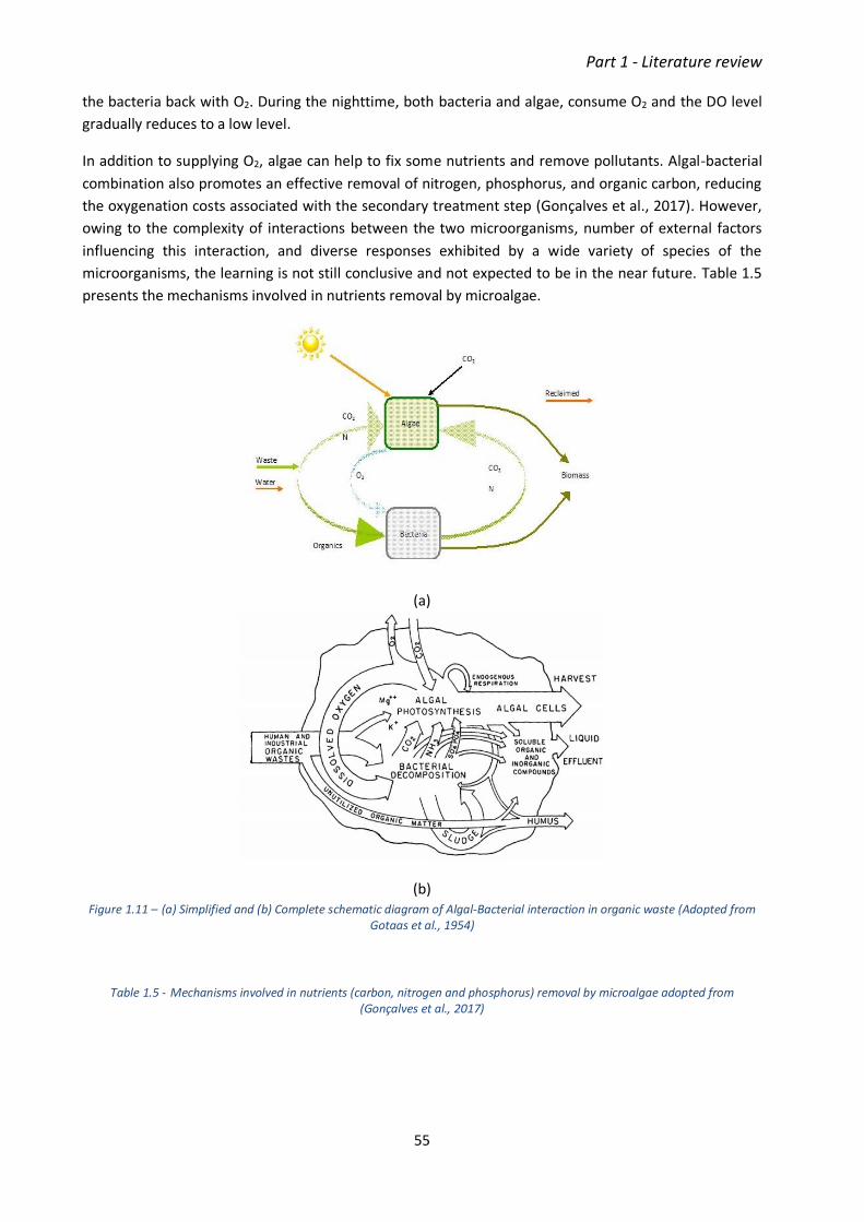
Part 1 - Literature review

55

the bacteria back with O2. During the nighttime, both bacteria and algae, consume O2 and the DO level

gradually reduces to a low level.

In addition to supplying O2, algae can help to fix some nutrients and remove pollutants. Algal-bacterial

combination also promotes an effective removal of nitrogen, phosphorus, and organic carbon, reducing

the oxygenation costs associated with the secondary treatment step (Gonçalves et al., 2017). However,

owing to the complexity of interactions between the two microorganisms, number of external factors

influencing this interaction, and diverse responses exhibited by a wide variety of species of the

microorganisms, the learning is not still conclusive and not expected to be in the near future. Table 1.5

presents the mechanisms involved in nutrients removal by microalgae.

(a)

(b) Figure 1.11 – (a) Simplified and (b) Complete schematic diagram of Algal-Bacterial interaction in organic waste (Adopted from

Gotaas et al., 1954)

Table 1.5 - Mechanisms involved in nutrients (carbon, nitrogen and phosphorus) removal by microalgae adopted from (Gonçalves et al., 2017)

Part 1 - Literature review

56

1.2.5.1 Sustainability

As mentioned in Section 1.1.4, sustainability needs to be a universal criterion for future projects in

general. By the same token, future wastewater treatment plants or more appropriately water resource

recovery facilities must be oriented from this perspective. As the new name infers, the fundamental

issues to be addressed from a sustainability point of view are reducing the energy consumption, the

recirculation of nutrients back to their natural system and production of useful materials from the

treatment byproducts. An exemplary practical achievement in this aspect is highlighted below.

An in-depth study is made by Grönlund et al., (2004) in an effort to make the first sustainability

assessment of wastewater treatment facility depending on microalgae. A microalgae wastewater

treatment plant model, designed to serve small size community (10,000 inhabitants) in small Swedish

town has been compared with conventional three-step WWTP and mechanical and chemical treatment

plant complemented by CWs (Grönlund et al., 2004). Two evaluation criteria, socio-ecological principles

and emergy analysis embraced by sustainability concepts, were used to assess the performance of the

three options. The score for the microalgae treatment method has significantly overtopped the other

two in terms of emergy analysis. This is due to the minimum energy requirement, use of local and free

environmental resources and biochemical content in the microalgae biomass to produce other

substances depending on the dominant species. When evaluated as per four pre-set socio-ecological

principles (concentrations of extracted substances from the earth’s crust, concentrations of produced

substances, physical degradation, and fulfilment of human needs world-wide) all three alternatives were

Part 1 - Literature review

57

scored equal against the three principles, and the microalgae treatment model has an advantage

according to the fourth principle. The detail is found in (Grönlund et al., 2004).

1.2.5.2 Economy and Methodology

Though related to sustainability parameter, economy and technical simplicity are specifically considered

as important constraints of plant effectiveness. Initial capitals, as well as operational expenditures of the

algal-bacterial integration treatment system, are very low in most cases. Aeration in the conventional

WWTP is an energy-intensive process taking up 45 to 75% of the plant operational cost (Panepinto et al.,

2016; Rosso et al., 2008). The presence of adequate microalgae in a wastewater treatment method is

analogous to the aeration system of conventional WWTP that eliminates an equivalent amount of

energy cost.

Irrespective of the highly complex process inside a reactor, the routine operation does not need expert

personnel. As also described in section 1.2.1.3.2, open ponds are usually a very suitable method for

mixing algae and wastewater. Hence, the big operational saving, in general, is due to the avoidance of

electromechanical devices and skilled manpower costs. Additional technical advancement could further

ease the operation and reduce associated costs.

1.2.5.3 Factors Affecting Algal-Bacterial Interaction in Wastewater

Factors influencing algal-bacterial interaction can be generally categorized into three main groups as

nutrient availability and distribution, environmental, and operational conditions. These factors

individually affect the natural metabolism of the two microorganisms, and they are also intertwined,

hence one factor changes the effect of the other.

1.2.5.3.1 Nutrients Availability and Distribution

Major nutrients needed by the algae and bacteria for their normal growth and multiplication are carbon,

nitrogen, and phosphorus. In the presence of sufficient oxygen, degradable organic carbon from the

wastewater is oxidized and consumed by heterotrophic bacteria. At the same time, inorganic carbon,

primarily CO2, is critically important for the productivity of algae in the wastewater. Algae take CO2 by

diffusion at low pH and part of their CO2 demand is supplied by heterotrophic bacterial oxidation of

organic carbon. Additional CO2 can be pumped in to enhance algal growth.

Similar to carbon, nitrogen is required by algae and bacteria as an important substrate of their growth

activity. Algae can use both forms of nitrogen, nitrate (NO3-) and ammonium (NH4

+) for their growth. In

the same way, bacteria also need nitrogen in the form of nitrate (NO3-) and ammonium (NH4

+) or

sometime in the form of nitrite (NO2-): heterotrophic bacteria assimilate ammonium to a certain extent

while nitrifying autotrophic bacteria oxidise ammonium into nitrite and nitrite into nitrate. In

wastewater, around 40% of nitrogen is in the form of NH4+ while the rest is mainly organic nitrogen

which is converted into ammonium by bacterial degradation, ammonification. In the case of

nitrification, most of the ammonium nitrogen will be converted to nitrate nitrogen leaving a small

portion remaining as ammonium and organic nitrogen. In the case of an algal-bacterial consortium with

photosynthetic aeration, ammonium nitrogen is oxidized to nitrite and then nitrate nitrogen by

nitrifiers. Since ammonium is the principal form of nitrogen in wastewater, ammonia inhibition could

impact the treatment process when dealing with high strength influent such as anaerobic digestion

centrate (Mantovani et al., 2019).

Part 1 - Literature review

58

As phosphorus also plays a vital role in every aspect of plant growth and development, the same is true

to algae in the form of orthophosphate (PO43-) for energy transfer, and biosynthesis of nucleic acids and

DNA (Richmond, 2008). Bacteria also use phosphorus while performing their normal metabolic process.

Fortunately, wastewater usually contains enough phosphorus in the form of orthophosphate,

polyphosphate or organic phosphate. In case of shortage, however, due to their high affinity for

inorganic nutrients, bacteria have a significant competitive advantage (Kisand et al., 2001) over other

organisms, particularly algae.

Beside the availability of the three important micronutrients, carbon, nitrogen and phosphorus, their

relative proportion, C:N:P ratio, also have an impact on the growth and composition of algal cell. The

C:N ratio of wastewater is generally low resulting in a low concentration of CO2 for the algal

photosynthetic process. Nitrogen and phosphorus limited conditions also cause the photosynthetic

process to be hindered. Some studies reported that the growth elements; lipid, fatty acids and protein

contents of certain species of algae, were impacted by N:P ratio variation (Rasdi and Qin, 2015). It was

also reported that a high C:N:P ratio in wastewater increased phosphorus removal and algal growth

while the low ratio (low carbon proportion) only increased nitrification (Cromar and Fallowfield, 1997).

Other organic and inorganic nutrients including pollutants are commonly found in wastewater. Despite

the difference in level, both bacteria and algae are tolerant to micropollutants (Tchobanoglus et al.,

2003). However, change in nutrient conditions of the substrate could lead to changing in bacterial-algal

interaction which could shift from synergistic to antagonistic interaction or vice versa (Grossart and

Simon, 2007).

1.2.5.3.2 Environmental Factors

Environmental conditions such as duration and intensity of light, temperature, pH, and dissolved oxygen

are equally important as that of nutrients for the desired interaction of algae and bacteria in wastewater

medium. One of the challenges in algal-bacterial interaction is adjusting the difference in the optimal

range of these environmental factors for the two major microorganisms.

Even though the duration and intensity of light optimum values vary between different species, it is a

prerequisite for microalgae to perform the photosynthetic process. A study by (Muñoz and Guieysse,

2006) indicated that the light intensity suitable in HRAP varies from 200 to 400 µEm-2s-1. Algae can adjust

themselves for natural light variation (photoacclimation) by changing the size and number of light

harvesting pigments or changing the distribution of harvested energy (Barsanti and Gualtieri, 2014). In

general, insufficient light ceases oxygen generation by photosynthesis while extended light supply

causes photoinhibition. Algal growth rate and nutrient removal efficiency are higher in intermittent

(light/dark) conditions than continuous light irradiance (Gonçalves et al., 2014).

Temperature variation in the culture directly affects the normal activities of both algae and bacteria. The

major problem with the open pond system in general and HRAP in particular is a lack of control on

temperature variation (Mata et al., 2010). At colder temperature carbon metabolism and nutrient

uptake (decrease of cells’ affinity to nitrate and ammonium) of an algal cell is lowered that eventually

affects photosynthesis (Reay et al., 1999). Certain species of algae can withstand very cold temperature,

however, (Park et al., 2011) suggested that optimum temperature for algal growth in wastewater varies

between 28 and 30°. On the other hand, temperature above the upper limit of the optimum range can

cause a more dramatic decrease in algal growth rate than cold conditions (Eppley, 1972). The effect of

temperature is multiplied as it also influences the solubility of oxygen and carbon dioxide which

Part 1 - Literature review

59

consequently changes the pH level to impact algal growth (Muñoz and Guieysse, 2006, p.). In addition,

algal cell size and its composition are also influenced by temperature (Richmond, 2008). Similarly,

temperature affects bacterial processes by influencing the enzymatic cellular reactions and the diffusion

of the external substrate into the cell (Grady Jr et al., 2011). Since nitrifying bacteria are living near the

free surface for aerobic conditions, they are sensitive to temperature variation and their performance

decreases significantly as the temperature goes down (Gerardi, 2003).

The pH of microalgal cultures is one of the most important factors that determine the interaction

between algae and bacteria. Nutrients removal such as carbon concentrating mechanisms adopted by

microalgal cells strongly depend on the pH, as pH determines CO2 solubility in the culture medium.

Excessive consumption of inorganic carbon by microalgae during photosynthesis disturbs the

equilibrium of CO2/HCO-3/CO2-

3 leading to an increase in pH level even above 11 (Park et al., 2011). pH

above 9 inhibits bacterial growth and decrease the nitrification process with an optimum range of 7.2 to

8 (Gerardi, 2003). High pH values are also responsible for NH4-N stripping and PO4-P precipitation

causing nutrient limitation for bacteria and algae (Yeoman et al., 1988).

Predation of microalgae and bacteria by zooplankton grazers is favoured by the presence of sufficient

food, oxygen and neutral pH condition inside the culture. Unless controlled by physical methods such as

filtration, hydrodynamic cavitation, and chemical methods such as injecting CO2, grazing can seriously

reduce the treatment efficiency of HRAP by changing the dominant algal species (Montemezzani et al.,

2017).

1.2.5.3.3 Operational Factors

Plenty of researches pointed out the effects of operational conditions such as hydraulic residence time

(HRT), mixing and depth of the culture on the algal production and treatment efficiency of HRAP.

Hydraulic residence time (HRT) of a system is the ratio of liquid volume in the system over liquid volume

removed from the system per unit of time (Von Sperling, 2007). Physical, chemical, and biological

processes in any type of reactor are highly dependent on HRT. In general, the HRT of a HRAP system

varies from 3-9 days (Sutherland et al., 2015a). Short HRT, not more than 4 days, resulted in higher algal

productivity (Park and Craggs, 2010) while long HRT, between 8 to 10 days, associated with better

nutrient removal and higher biomass concentration (Cromar and Fallowfield, 1997). For an effective use

of reactors and efficient nutrient removal, Matamoros et al., (2015) suggested to adjust HRT based on

the seasonal change by reducing HRT for spring and summer and increasing HRT for autumn and winter.

Hydrodynamic mixing plays a vital role in algal-bacterial interaction in wastewater culture since it also

affects the previous two factors, nutrient distribution and environmental conditions directly or

indirectly. In HRAP, mixing is achieved by paddlewheel rotation which circulates the culture along the

channel thus creating micro-turbulence (Park et al., 2011). Mixing prevents algal sedimentation that

may lead to organic matter accumulation at the bottom of the pond leading to decreasing algal

exposure to light while promoting anaerobic conditions and toxic compounds release (Andersen,

2005a). Mixing even out heat, gas and nutrient gradients and enhances mass transfer rate between cell

and culture medium (Grobbelaar, 1991). Vertical mixing is of paramount importance for algal cells to

oscillate in the light/dark cycle. Particularly in long HRAP, vertical mixing is very poor especially in the

straight channel section (Hreiz et al., 2014a). Higher velocity may be induced to generate strong mixing.

This may cause, however, mechanical damage on algal cells from high shear stress and an increase in

energy consumption (Kumar et al., 2015).

Part 1 - Literature review

60

HRAP is in general characterized by a shallow operating depth ranging from 0.1 to 0.3m. Increasing or

decreasing the depth of the culture has both positive and negative effects on the productivity of the

pond as reported by Sutherland et al., (2014). When the depth is increasing the shadow effect of the

algal biomass by absorption and scattering will be pronounced (Grobbelaar et al., 1990), reducing light

penetration (Andersen, 2005a). The increasing water level also leads to higher energy consumption per

unit area (Hadiyanto et al., 2013). On the other hand, a smaller depth of water in the reactor causes a

higher temperature gradient (Kumar et al., 2015) leading to excess evaporation. And from an economic

point of view, the low water level needs a bigger size of the pond if a stable HRT is required.

1.2.6 Perspectives for research concerning algal/bacterial treatment of wastewater

It was mentioned in the previous chapter that present and future wastewater treatment plants need to

be oriented not only from treating the polluted water perspective but from recovering the useful

constituents’ standpoint also. Wastewater contains various important micronutrients and inherent

energy in the organic matter. The big challenge not resolved acceptably even for the state of the art is

concentrating and recovering these resources. At present, several methods are available to partly

achieve this noble objective. A combination of microalgae and bacteria offer various attractive

advantages over conventional wastewater treatment systems. However, the complexity of interaction

between the two characteristically different microorganisms, and the number of environmental and

operational factors are allegedly demanding intensive efforts and additional tools to adequately address

the issue.

The curiosity to fully understand the detail phenomena and the endeavor to maximize the benefit

without impacting the environment is yet an active research interest. On this behalf, to enhance the

energy recovery from wastewater, keeping in mind the limited information to optimize algal-bacterial

interaction, a recent innovative method that integrates algal-bacterial community with the

photobioelectrochemical system has been suggested (S. Luo et al., 2017). In such a system, algae

contribute to the bioelectrochemical system function as an organic feedstock to support bacterial

growth, by assisting anode bacteria to generate electricity, by providing oxygen from photosynthesis as

a cathode electron acceptor, and by removing N and P from the wastewater. (S. Luo et al., 2017)

recommends a clear understanding of the critical microbial processes such as algal photosynthetic and

nutrient metabolism and collaborative/competitive relationships between algae and bacteria will help

to improve the energy recovery using such device.

The poor settleability of microalgae, due to small size, low cell density and negative charge of the cell

surface that prevents microalgal aggregation (Uduman et al., 2010), impaired the harvesting of algal

biomass from the culture solution. It is still a bottleneck on the cost-effectiveness of the HRAP engaged

in mass production for biofuel or other purposes (Quijano et al., 2017). In the case of wastewater

treatment, bacteria produce extracellular polymeric substances that play a key role to mediate their

aggregation with microalgae and cyanobacteria (De Schryver et al., 2008). This resulted in an increase of

the aggregate size from 50μm up to 5000μm, depending on the operating conditions and other

organisms such as protozoa and small metazoans in the surroundings of the aggregate have been

consistently observed during wastewater treatment (De Schryver et al., 2008). Despite the need for

further research to fully understand the fundamentals underlying the formation of microalgal-bacterial

aggregation and their performance, it has encouraged the use of algal-bacterial based wastewater

treatment (Quijano et al., 2017).

Part 1 - Literature review

61

Figure 1.12 - Simplified schematic representation of CO2 and O2 mass transfer in the extracellular polymeric film of thickness δ between microalgae and bacterial cells in microalgal bacterial aggregate (Quijano et al., 2017).

While the computing power and storage capacities are ever-increasing, the use of numerical models is

currently becoming a popular and potentially viable option to simultaneously study the complex

biochemical kinetics and hydrodynamics inside a reactor like HRAP. This frame of approach is allowing a

better understanding of the system for estimation of effluent quality and final biomass production, and

for optimal design and control (Solimeno and García, 2017). Since the first integrated mathematical

model that considers the simultaneous growth of microalgae and bacteria by (Buhr and Miller, 1983a),

numerous advanced models evolved from steady-state to dynamic character are available at present for

an improved prediction of algal-bacterial interaction (Solimeno and García, 2017). These models are

becoming increasingly complex and comprehensive regarding the biochemical processes occurring.

However, the previous sections also highlight the importance of hydrodynamics and mixing for the

operation of a HRAP. Therefore, a relevant mathematical model of a HRAP should also describe

hydrodynamics with the same level of precision. In this respect, Computational Fluid Dynamics is

nowadays a relevant tool for optimizing bioreactors design and operation but also for integrating with

other biochemical and physical (gas-liquid mass transfer) sub-models.

Part 1 - Literature review

62

1.3 Computational Fluid Dynamics (CFD)

Computational fluid dynamics (CFD) consists of the numerical analysis of problems involving fluid flows.

The aim is to simulate the motion of the fluid in interaction with specific conditions defined at system

boundaries (surfaces). According to the objective, additional equations accounting for heat transfer or

even chemical reactions can be coupled to the governing equations for fluid flow. In the wastewater

treatment field, Larsen, (1977) is considered as the pioneer using this tool.

In classical CFD, the continuous fluid domain is discretized as a mesh/grid containing smaller sub-

volumes called cells or control volumes. The governing equations (conservation laws for mass,

momentum and heat transfer) are integrated using discretization algorithms over each cell.

1.3.1 Navier-Stokes equations: continuity and momentum

The Navier-Stokes equations are the basic model for fluid motion. They combine a continuity equation

with a transport equation for momentum as follows (Andersson et al., 2011):

The continuity (i.e. mass conservation) equation is as following (Equation 1-1):

∂ρ/ ∂t + ∇ ⋅ (ρ�� ) = 0

Equation 1-1

where �� is the velocity and ρ is the fluid density.

The first term in the left side is the rate of change in time of the density while the second term

represents the flow of mass out of the element across its boundaries (convective term). In the case of an

incompressible fluid, density does not evolve with time and its derivative thus becomes 0. Equation 1-1

thus turns to:

∇ ⋅ (�� ) = 0

Equation 1-2

In Cartesian coordinate system, this is decomposed in to:

∂𝑢

∂𝑥= 0

∂𝑣

∂𝑦= 0

∂𝑤

∂𝑧= 0

Equation 1-3

Momentum equations are the following (Equation 1-3, Equation 1-4, Equation 1-5) in the case of an

incompressible flow with constant viscosity. The rate of increase of momentum of a fluid particle is

equal to the sum of surface and body forces on a fluid particle. Surface forces include viscous and

pressure while body forces include gravity, centrifugal, Coriolis or even electromagnetic forces when

considered. The terms 𝑆𝑀𝑥 , 𝑆𝑀𝑦 and 𝑆𝑀𝑧 are the body forces with 𝑆𝑀𝑦 is equal to −𝜌𝑔 when the gravity

is considered. Considering u, v, and w as the components of velocity �� in x, y and z directions

respectively (assuming an incompressible Newtonian flow with constant density and viscosity):

Part 1 - Literature review

63

∂u

∂t+ u

∂u

∂x+ v

∂u

∂y+ w

∂u

∂z= −

1

𝜌

∂p

∂x+ υ (

∂2𝑢

∂x2+

∂2𝑢

∂y2+

∂2𝑢

∂z2) + SMx

Equation 1-4

∂v

∂t+ u

∂v

∂x+ v

∂v

∂y+ w

∂v

∂z= −

1

𝜌

∂p

∂y+ υ (

∂2v

∂x2+

∂2𝑣

∂y2+

∂2𝑣

∂z2) + SMy

Equation 1-5

∂w

∂t+ u

∂w

∂x+ v

∂w

∂y+ w

∂w

∂z= −

1

𝜌

∂p

∂z+ υ(

∂2𝑤

∂x2+

∂2𝑤

∂y2+

∂2𝑤

∂z2) + SMz

Equation 1-6

Where p is the pressure, ν =μ

ρ is the kinematic viscosity and µ is the dynamic viscosity.

To simplify the writing of these equations, one can use the index notation: j should be summed over all

dimensions, i.e. j = 1, 2 and 3, and i appears in all terms and for three dimensions (Andersson et al.,

2011):

𝜕𝑈𝑖

𝜕𝑡+ 𝑈𝑗

𝜕𝑈𝑖

𝜕𝑥𝑗= −

1

𝜌

𝜕𝑃

𝜕𝑥𝑖+ 𝜐 (

𝜕2𝑈𝑖

𝜕𝑥𝑗2 ) + 𝑆𝑀𝑖

Equation 1-7

As it is not in the scope of the present study, heat conservation equation is not presented.

1.3.2 Turbulence model

Turbulence characterizes the fluid flow where the velocity displays random three-dimensional vorticity

at any point: size, location and orientation of vortices are constantly changing. Turbulent flows are

therefore characterized by a behavior that is difficult to predict and the existence of many spatial and

temporal scales. Such flows occur when the kinetic energy moving the fluid (inertia forces) is relatively

intense in comparison to the viscous forces opposing to fluid motion. This is expressed by the

dimensionless ratio called Reynold number:

Re =ρ𝑈𝐷

μ

Equation 1-8

where ρ is the density of the fluid, U is the average velocity, D is the characteristic length and μ is the

dynamic viscosity of the fluid.

Most flows encountered in engineering applications are turbulent. This is the case in biological reactors

used as WRRFs. In turbulent flow, measurement of velocity at one point exhibits the following form

(Versteeg and Malalasekera, 2007):

Part 1 - Literature review

64

Figure 1.13 - Measurement of velocity in turbulent flow (Versteeg and Malalasekera, 2007)

In this situation, the velocity is decomposed into an average constant value U and a fluctuating

component u’(t) (Equation 1-9). This is the same for the components v and w in y and z directions.

Ui(𝑡) = Ui + ui′(𝑡)

Equation 1-9

The derivation of momentum equations in that case yields the Reynolds Averaged Navier-Stokes (RANS)

equations (Equation 1-10):

𝜕𝑈𝑖

𝜕𝑡+ 𝑈𝑗

𝜕𝑈𝑖

𝜕𝑥𝑗= −

𝜕��

𝜕𝑥𝑖+

𝜕

𝜕𝑥𝑗(𝜇

𝜕𝑈𝑖

𝜕𝑥𝑗− 𝜌𝑢𝑖𝑢𝑗 ) + 𝑆𝑀𝑖

Equation 1-10

These equations have the same form than the original momentum equation except the presence of the

extra turbulent stresses. It is derived from the Reynolds stresses defined as 𝑅𝑖𝑗 = −ρ𝑢’𝑖𝑢’𝑗 e.g. 𝑅𝑥𝑦 =

−ρ𝑢’𝑣’ .

These Reynolds stresses are six additional unknowns in the equations. The role of turbulence models is

therefore to derive phenomenological functions to close this set of equations. The RANS models predict

the Reynolds stresses and the associated scalar transport terms. They can be classified as follows

(Versteeg and Malalasekera, 2007):

• Zero equation model: Mixing length model

• One equation model: Spalart-Allmaras model

• Two equations models: 𝑘 − ϵ; 𝑘 − ω

• Reynolds stress equation model (RSM)

• Algebraic stress models

• Large Eddy Simulation (LES)

Part 1 - Literature review

65

The RSM models are more accurate than the two-equation models. However, they are computationally

intensive as they solve one partial differential equation for each one of the six independent Reynolds

stresses.

Mixing-length and 2-equations models are the most used types for engineering purposes. They are

introducing the concept of turbulent (or eddy) viscosity based on analogy between viscous stresses and

Reynolds stresses (Equation 1-11). Boussinesq suggested this approach to describe the influence of the

fluctuating parameters.

−𝜌𝑢𝑖𝑢𝑗 = 𝜇𝑡 (𝜕𝑈𝑖

𝜕𝑥𝑗+

𝜕𝑈𝑗

𝜕𝑥𝑖) −

2

3𝜌𝑘𝛿𝑖𝑗

Equation 1-11

where k is the turbulence kinetic energy and 𝛿𝑖𝑗the Kronecker delta (equal to 1 if i=j and 0 elsewhere). A

kinematic turbulent viscosity is defined as ν𝑡 =μ𝑡

ρ. Hence, the momentum equations for incompressible

flow become (Equation 1-12):

𝜕𝑈𝑖

𝜕𝑡+ 𝑈𝑗

𝜕𝑈𝑖

𝜕𝑥𝑗= −

1

𝜌

𝜕��

𝜕𝑥𝑖+

𝜕

𝜕𝑥𝑗[(𝜈 + 𝜈𝑡) (

𝜕𝑈��

𝜕𝑥𝑗+

𝜕𝑈��

𝜕𝑥𝑖)] −

2

3

𝜕𝑘

𝜕𝑥𝑖+ 𝑆𝑀𝑖

Equation 1-12

The kinetic energy K per unit mass is defined by Equation 1-13 (Versteeg and Malalasekera, 2007):

𝑘 =1

2(𝑢‘2 + 𝑣‘2 + 𝑤‘2 )

Equation 1-13

Hence the turbulence model can be seen as the set of equations that are needed to determine the

turbulent viscosity (Andersson et al., 2011). In the following sections, the most common 2 equations

models used in the field of wastewater engineering are presented. These Two-equation models allow

the determination of both turbulent length and time scales (ANSYS FLUENT 12.0, 2009) by solving two

separate transport equations.

1.3.2.1 Standard k- model

The k- model allows to describe the effect of turbulence properties on the mean flow as well as the

production and destruction of turbulence. This model is proper for fluids where convection and diffusion

cause significant differences between production/destruction of turbulence (e.g. recirculating flows).

The flow is assumed to be fully turbulent, and the effects of molecular viscosity to be negligible. This

model is therefore valid only for fully turbulent flows.

The model is focused on the mechanism that affects the turbulent kinetic energy (k). Two transport

equations are solved for turbulent kinetic energy k and its rate of dissipation :

∂(ρ𝑘)

∂𝑡+ ∇ ⋅ (ρ𝑘𝑣 ) = ∇ ⋅ [

ν𝑡

σ𝑘∇𝑘] + 2ν𝑡𝑆𝑖𝑗. 𝑆𝑖𝑗 − ρ

Equation 1-14

Part 1 - Literature review

66

∂(ρϵ)

∂𝑡+ ∇ ⋅ (ρϵ𝑣 ) = ∇ ⋅ [

ν𝑡

σϵ∇ϵ] + 𝐶1ϵ

ϵ

𝑘2ν𝑡𝑆𝑖𝑗. 𝑆𝑖𝑗 − 𝐶2ϵρ

ϵ2

𝑘

Equation 1-15

Where ν𝑡 is the eddy viscosity, and 𝑆𝑖𝑗 the rate of deformation. The eddy viscosity is assumed isotropic

and computed as follows:

μ𝑡 = ρ𝐶μ

𝑘2

ϵ

Equation 1-16

The dimensionless constants of the model are:

Table 1.6 - Constants of k- model

Constant Value 𝑪𝛍 0.09

𝛔𝒌 1.00

𝛔𝛜 1.30

𝑪𝟏𝛜 1.44

𝑪𝟐𝛜 1.92

1.3.2.2 RNG k- model

The main difference with the standard model is a different formulation of the dissipation equation

which includes an additional source-term. Regions with large strain rate, smaller destruction of ϵ will

occur due to this source term: ϵ increases and k reduces. In turn, the effective viscosity decreases. This

should yield improvements in prediction of swirling flows and flows in which the geometry displays

strong curvature. However, the predictions will be inferior to standard k-ϵ model for jets and plumes

(Andersson et al., 2011).

1.3.2.3 Realizable k- model

The realizable k-ϵ model (Shih et al., 1995) differs from the standard model by two different ways:

• Alternative formulation for the turbulent viscosity.

• Modified transport equation for the dissipation rate, ϵ

The term “realizable” implies that the model satisfies certain mathematical constraints on the Reynolds

stresses, consistent with the physics of turbulent flows.

In the realizable k–ε model, Cμ is variable: it is a function of the local state of the flow to ensure that the

normal stresses are positive under all flow conditions (Andersson et al., 2011).

1.3.2.4 K-omega and k-omega SST models

The second widely used two-equation model, introduced by Wilcox, (1998), is the k-ω model. It also

assumes an isotropic eddy viscosity. Here, the turbulent viscosity is computed as a function of k and the

specific dissipation ω with

Part 1 - Literature review

67

ω =ϵ

k

Equation 1-17

Equation 1-16 thus becomes:

μ𝑡 = ρα∗𝑘

ω

Equation 1-18

where α∗ is a coefficient damping the turbulent viscosity causing a low-Reynolds-number correction.

This value is computed as:

α∗ = α∞∗ (

α0∗ + 𝑅𝑒𝑡/𝑅𝑘

1 + 𝑅𝑒𝑡/𝑅𝑘)

Equation 1-19

where:

𝑅𝑒𝑡 =ρ𝑘

μω

𝑅𝑘 = 6

α0∗ =

β𝑖

3

β𝑖 = 0.072

This model displays better performance than k-ϵ model in regions with low turbulence. In the viscous

sub-layer into the near-wall area, this model also eliminates the need for use of wall-functions, provided

the use of a very fine mesh close to the wall (Andersson et al., 2011; Karpinska and Bridgeman, 2016).

The shear-stress transport (SST) k-ω model (Menter, 2012) combines the formulation of k-𝜔 model in

the near-wall region with the free-stream independence of k-𝜖 model in the far field: both models are

added together and multiplied by a blending function (one in the near-wall region to activate k-𝜔 model

and 0 away from the surface to activate k-𝜖). The definition of the turbulent viscosity is also modified.

This model is considered to be the most accurate from two-equation eddy viscosity models (Karpinska

and Bridgeman, 2016).

1.3.3 Multiphase flow

In wastewater treatment applications, several phases interact and have to be considered in the model.

Depending on the application and simplifications to be made, several situations can be described. These

usually include:

1. Gas-liquid phases: the two main situations where this can occur are:

a. the open-channel flow (stratified) where one wants to track the position of the interface

(free surface);

Part 1 - Literature review

68

b. the description of interacting phases such as in fine bubble aeration or fate of biogas in

anaerobic digesters;

2. Liquid-solid phases: this is the case in biological reactor where water is the continuous phase

and activated sludge is the dispersed (solid) phase.

The different approaches allowing to represent these situations are described in the following

subsections.

1.3.3.1 Euler - Lagrange model

This approach is adapted for simulating liquid/solid suspensions when the dispersed phase does not

impact the bulk fluid motion. This is usually the case in grit removal processes or settlers used to treat

combined sewer overflows (Isenmann, 2016). The fluid phase is described as a continuum while the

dispersed phase (solid particles or droplets) is represented by many particles that are tracked

throughout the flow domain. To be applied in a reliable way, the dispersed phase must be maximum 10-

12 % (De Clercq et al., 2005). This approach can also involve a very high computational cost when the

number of individual particles to follow increases (Wicklein et al., 2015).

1.3.3.2 Euler-Euler model

In this approach, the two phases are treated as continuous media. Continuity and momentum equations

are solved for both phases. Volume fractions of each phase as well as the exchange of momentum and

mass between the phases are described. For the latter, empirical information is required to close the

momentum equations (Andersson et al., 2011). This approach could be applied for bubbly flows (Amato

and Wicks, 2009; Wicklein et al., 2015).

The volume fraction of the dispersed phase is defined as follows (Equation 1-20):

αd =∑ ViNd

i=1

V

Equation 1-20

Where Vi is the volume occupied by particle or droplet i and Nd is the total amount of particles or

droplets present in volume V.

1.3.3.3 Volume-Of-Fluid (VOF) approach

This approach is a Euler-Euler model with a fixed grid (mesh). It is used to simulate free surface flows or

bubbly flows. The interface between the phases is tracked. It is suitable in the case of immiscible fluids

with clearly defined interface. Some classical applications are motion of large bubbles in a liquid, motion

of liquid after a dam break and more generally steady or transient tracking of any liquid-gas interface. In

the case of bubbles, the bubble size must be significantly larger than a control volume.

Each cell is assumed to contain only one phase or the interface between them. A single set of

momentum equations is solved. Additional source terms are included to account for surface tension and

wall adhesion. A volume fraction conservation equation is solved for each phase (Equation 1-21) while

only one set of momentum equation is solved.

Part 1 - Literature review

69

∂α𝑑

∂𝑡+ 𝑢𝑗

∂α𝑑

∂𝑥𝑖= 𝑆α𝑑

Equation 1-21

This volume fraction can take values with three possible situations:

• 0 if the cell is empty of the secondary fluid;

• 1 if the cell is full;

• Between 0 and 1 if the cell contains the interface.

Usually, the source-term 𝑆α𝑑 takes a zero value but mass transfer between phases can be modelled by

specifying a non-zero value for it.

1.3.3.4 Mixture (drift-flux) model

This model can be applied to describe two interpenetrating phases which are then considered as a single

mixture instead of two different phases. It is suitable to describe flows with strong coupling and moving

with almost the same velocity. A single set of Navier-Stokes (mixture continuity and momentum) based

on the mixture center of mass is solved. The dispersed phase volume fraction is included as a variable of

the model and its transport is modelled by a convection-diffusion equation accounting for the relative

velocity e.g. settling velocity. In the wastewater treatment field, this model has mainly been applied for

describing activated sludge sedimentation (Brennan, 2001; Valle Medina and Laurent, 2020).

1.3.3.5 Euler - transport model

For solids transport, most of the simulation models, essentially applied for sludge sedimentation

processes, consider the solid phase (sludge) as a scalar for example in (De Clercq, 2003; Griborio, 2004;

Lakehal et al., 1999). The fluid phase is described as a continuum with both continuity and momentum

equations solved. The dispersed phase motion is described by a scalar transport equation (Equation

1-22) that uses the computed flow field for the advective term:

∂𝑋

∂𝑡+ ∇ ⋅ [(�� + υ𝑠 )𝑋] = ∇ ⋅ (𝐷𝑚 +

ν𝑡

𝑆𝑐𝑡∇𝑋)

Equation 1-22

Where X is the concentration of the dispersed phase, vs is the settling velocity modeled by empirical

relations (Torfs et al., 2017), Dm is the molecular diffusion coefficient and Sct is the turbulent Schmidt

number.

This equation and its parameters will be further discussed in section 1.5 (page 76). In order to take into

account the interactions between phases, specific relations for viscosity (e.g.(BOKIL and Bewtra, 1973;

Locatelli et al., 2013)) and density (Samstag et al., 2012; Wicklein and Samstag, 2009) coupling between

the phases have to be included.

1.4 State of the Art in Application for High-Rate Algal Ponds

High-Rate Algal Ponds usually use channels with constant width and depth, curved bends at each

extremity, and one or more paddle wheels to circulate water through the system. In this system, most of

the energy loss occurs at the curved “hairpin” bends (Liu and Zhang, 2019) (see section 1.2.2 p 49).

Part 1 - Literature review

70

As stated earlier, CFD is a tool that can allow to evaluate the HRAP designs and to produce new designs

which may reduce this energy loss as well as providing better vertical mixing that can optimize algal cells

access to light, reduce sedimentation and improve gas/liquid transfer rates.

One of the challenges, for a system having a rotating element in general and for HRAP in particular, is

the representation of the momentum induced by the rotating paddlewheel that is usually in charge of

inducing mixing and liquid velocity in such systems. Inlet Velocity and Dynamic Mesh are the two

common CFD methods to simulate rotating elements (Amini et al., 2016). The most comprehensive one

is the Dynamic Mesh that considers the rotation of the paddle-wheel geometry and simulates the

momentum transferred to the fluid through the rotating mesh (Hreiz et al., 2014b). In this method,

linear motion or rotation of a solid body, based on the physical phenomenon, is handled by a moving or

rotating mesh with or without mesh morphing within the specified boundaries. However, this approach

could be computationally intensive particularly when the model is intended to be integrated with other

models such as biokinetics, gas transfer, and light irradiance models.

Depending on the modelling objective, one can consider simplifying the simulation replacing the paddle-

wheel by introducing a momentum source term in the governing equation or by assigning a constant

inlet velocity on a virtual inlet boundary (Hadiyanto et al., 2013). The latter one is even easier; it can be

used to model passive scalar transport of tracer material by applying cyclic inlet and outlet boundaries.

This method assumes a steady-state flow and therefore flow fields are calculated from a steady-state

simulation.

Table 1.7 summarizes the different published CFD studies in literature.

1.4.1 Moving elements/rotation description

Due to a wide range of engineering applications, analyzing flow around a rotating element is required in

many cases including pumps, water turbines, wind turbines, aircraft engines, chemical reactors, and

processing equipment. The hydrodynamics inside a HRAP is also conducted in the rotating regime

caused by the paddlewheel. However, the comprehensive treatment of such components in CFD is

demanding in terms of model building as well as computational resource (Amini et al., 2016) since a

specific numerical approaches for the modelling of complex flow systems containing rotating parts is

needed (Wilhelm, 2015). Hence, various simplifications have been developed to simulate fluid flow

problems consisting of rotating device. Some of the common methods are briefly described below.

1.4.1.1 Momentum source

The first option to model the effect of rotational elements such as paddlewheel, fans and ventilators

that adds in momentum gain of a system is by introducing a source term in the governing equations.

This option allows modeler to define a volume in the system domain which generates momentum,

without any further complication of providing detailed geometry and finer mesh of the rotating

elements. The known velocity output (with its correct x, y, and z components) and dimension of a

rotating device can be assigned to an identical shaped volume (box, sphere, cylinder or cell zones) at

similar location in the computational domain. This method can be used for the analysis of various flow

problems except compressible and multiphase flows. It is also limited to implement the average velocity

that could hide some reality.

Part 1 - Literature review

71

OpenFOAM provides a flexible framework to add various source terms including heat and momentum in

to the governing equation through “fvOptions” file in the system directory without rewriting the original

source code (OpenCFD, 2011). An equivalent momentum source is added to adjust the average velocity

in the whole domain or user-specified cellZone or cellSet to the desired value.

1.4.1.2 Specific boundary condition: Inlet Velocity approach

Another simplified approach to represent the rotational elements in CFD models is the Inlet Velocity

method. Based on the flow direction, a virtual inlet and outlet boundaries are provided replacing the

rotating device with an average velocity from this device prescribed on the inlet boundary. A small

physical gap is needed between the two boundaries to realize the simulation. In the case of solving

transport equations, cyclic boundary condition is set between the inlet and outlet face to ensure the

swapping of transported materials. This method assumes a steady-state condition that makes it more

suitable when a steady-state physical flow field solution is expected. In this study, Inlet Velocity

approach is tested and compared with the Dynamic Mesh method.

1.4.1.3 Single Reference Frame (SRF)

Moving reference frame in general is advantageous to reduce a flow problem which is unsteady in the

stationary (inertial) frame to a steady type with respect to the moving frame (ANSYS FLUENT 12.0,

2009). For a steadily rotating frame (i.e., constant angular speed), it is possible to transform the

governing fluid flow equations to the rotating frame such that steady-state simulations are possible.

Hence, fluid flow around a rotating device can be modeled using a single rotating frame of reference

(SRF) that adheres to the rotating machinery when only one rotating flow domain is considered. Since

steady-state condition is assumed without any mesh motion, where the complete computational fluid

region is in motion, SRF simulations are computationally less costly and are therefore predestinated for

elaborated multi parameter studies (Wilhelm, 2015). Nevertheless, the assumptions made in this

method could compromise the result to a certain degree depending on the complexity of the problem.

1.4.1.4 Multiple Reference Frame (MRF)

Rotating flow applications commonly involve both steady and unsteady flow regions. SRF cannot handle

if the computational domain incorporates stationary and moving zones at a time. MRF overcome this

drawback and enables to simulate two or more subdomains in which either of them may be stationary

or in motion (Wilhelm, 2015). A virtual Arbitrary Mesh Interfaces (AMI), that has no physical meaning

but exclusively used for numerical simulations to exchange calculated flow field information at each

iteration steps, are introduced to connect the different regions (Dellinger et al., 2018; Greenshields,

2018). However, proper positioning of these interfaces in the geometry and the generation of a smooth

mesh on both sides of the AMI is the challenging task of the MRF method (Wilhelm, 2015). The higher

the smoothness and uniformity of the cell size on both side of the AMI, the better is the quality of the

result (Wilhelm, 2015).

MRF can be implemented in two ways, Frozen Rotor Technique and Mixing Plane Approach. Both

methods perform a steady-state simulation. However, the first one solves the governing equation for

one rotor position, normally very quick simulation, and converges to a snapshot of the fluid flow system.

Part 1 - Literature review

72

It is possible to conduct the simulation at several rotor positions and average integral quantities

(Wilhelm, 2015). OpenFOAM uses SIMPLE solver algorithms to employ this option.

Mixing Plane approach is an improvement on Frozen Rotor technique that gives a better approximation

of circumferential average of all flow quantities in the internal interface called mixing plane in a much

less computational time compared to unsteady simulation. But local flow information such as local

vortices are spread out over the mixing plane in which the results show only an averaged value not

based on a physical time step (Wilhelm, 2015).

For a rotating (non-inertial) coordinate system on the rotor, the flow is usually steady relative to the

rotating frame. Conversely, the rotor and the flow around the rotor are unsteady with respect to the

fixed (inertial) reference. Under properly prescribed interface condition, the Navier-Stokes equations

are solved independently for both subdomains. The equation is modified and solved for the rotating

region based on the moving frame incorporating two additional force terms, Coriolis and Centrifugal,

which occur due to the transformation from the stationary to the moving reference as shown in

Equation 1-23.

∂(𝜌𝑢𝑟)

𝜕𝑡+ ∇ ∙ (𝜌𝑢𝑟𝑢𝑟) + {2𝜌𝛺 × 𝑢𝑟} + {𝜌𝛺 × (𝛺 × 𝑟)} = −∇𝑝 + ∇ ∙ (𝜇∇𝑢𝑟)

Equation 1-23

∂(𝜌𝑢)

𝜕𝑡+ ∇ ∙ (𝜌𝑢𝑢) = −∇𝑝 + ∇ ∙ (𝜇∇𝑢)

Equation 1-24

𝑢𝑟 = 𝑢 − 𝛺 × 𝑟

Equation 1-25

The third and the fourth term inside the curly bracket of Equation 1-23 are the Coriolis and centrifugal

force components respectively. For the stationary subdomain, Equation 1-23 is reduced to Equation

1-24 avoiding the relative term. In both equations p, ρ, μ and ur stands for pressure, density, dynamic

viscosity and relative velocity respectively. And 𝛺 is rotation vector and r is the position vector. Relative

velocity is calculated as per the Equation 1-25.

Nonetheless, MRF method implemented in OpenFOAM can only handle fluid motion when the angular

speed of the rotating reference is constant. Hence, MRF model computes steady-state solution for fluid

flow problems using both rotating and stationary frame of reference. Moreover, versions earlier than

OpenFOAM 5.0 deal only with rotations but not translational movement. Other commercial packages

like ANSYS FLUENT have this capability.

1.4.1.5 Moving Mesh

Both SRF and MRF methods described above neglect the unsteadiness of the fluid motion and provides a time-averaged solution. Unsteady flow simulation or a time-accurate solution for rotor-stator interaction can be computed by Moving Mesh modules (ANSYS FLUENT 12.0, 2009). Although these techniques are computationally very intensive, for highly transient rotational flow, they are the most accurate option for simulating flows in multiple moving reference frames. Similar to the MRF case above, for the static and rotating subdomains, the governing flow equations are solved separately.

Part 1 - Literature review

73

In CFD modelling, Moving Mesh can be implemented in two slightly different styles, Sliding Mesh and

Dynamic Mesh, both simulating unsteady conditions. Sliding Mesh is suitable when there is a transient

rotor-stator interaction in the computational domain (ANSYS FLUENT 12.0, 2009). It allows adjacent

grids to slide relative to each other along the mesh interface surface. Sliding Mesh method considers

cells are transferred by the motion without changing their original topology (size and shape) within a

fixed boundary: i.e the control volume remains constant. Hence, this method is more appropriate to

model when the flow is not subjected to excessive deformation.

While the rotation or translation takes place, as long as the two AMI boundaries are based on the same

geometry and finely meshed for a smooth slip, cell alignment along the arbitrary interface is not

required. Since the flow is inherently unsteady, a time-dependent solution procedure is applied (ANSYS

FLUENT 12.0, 2009) while coupling between the two regions is achieved by interpolating the flow

variables on the cell faces (Wilhelm, 2015).

Model construction of Dynamic Mesh is similar with Sliding Mesh technique. However, the Dynamic Mesh solver is capable of modelling fluid flows subjected to a change in shape and volume of the domain with time due to motion of one or more boundaries. Hence, following the new position of the moving boundaries, the position and shape of the grid cells are updated or adjusted accordingly at each time step. The process of updating mesh topology obviously makes the calculation extremely intensive even to small grid size. This method can be used to model boundaries moving rigidly relative to each other. A good example is the compression of fluid by piston inside a cylinder. And it can also be used for deforming boundaries such as modelling inflation of a balloon.

Using OpenFOAM, in this study, Dynamic Mesh method is applied to simulate the hydrodynamics of lab

scale HRAP consisting of a rotating paddlewheel. In OpenFOAM, both Sliding Mesh and Dynamic Mesh

methods employ the PIMPLE solver algorithm to obtain an unsteady solution that requires much larger

computational time than the MRF technique.

1.4.2 Experimental validation

The CFD model of HRAP often includes some simplifications of the geometry (e.g. for paddlewheel) and

the choice of turbulence model is also of significance. Model validation with experimental data is

therefore required. This is often carried out by means of velocity measurements (see Table 1.7) and

tracer tests. The latter is an approach very well established in chemical engineering. However, its use to

evaluate a CFD model and simulate contaminants transport must consider some important elements

regarding both experimental and numerical procedures. This is discussed in the next section.

Part 1 - Literature review

74

Table 1.7- CFD modelling of High-Rate Algal Ponds

Reference Code Scale Mesh size and

type

Turbulen

ce

Multiphase

approach

Approach for

paddle-wheel

Extra-

model

Experimental

validation? Outcome

(Liffman et al., 2013) ANSYS CFX 12 Pilot-scale

Unstructured

tetrahedral

(1,000,000 cells)

or hexahedral

(300,000 cells)

k–e Single phase Momentum

source No No

Geometric

modification

of HRAP

(Hadiyanto et al., 2013)

COMSOL

Multiphysics v.

3.4

Pilot-scale - k–e Single phase Inlet Velocity No No

Geometric

modification

of HRAP

(Hreiz et al., 2014a) ANSYS 13 Fluent Pilot-scale

Structured

hexahedral

dominant

(310,00 cells)

Realizable

k-e VOF Sliding mesh No

Tracer test +

Doppler

Velocimetry

Modification

s of paddle-

wheel

design

(Huang et al., 2015) ANSYS CFX 12.1 Lab-scale Hexahedral

(380,000 cells) k–e VOF Sliding mesh No PIV

Geometric

modification

of HRAP

(Park, 2014) ANSYS Fluent

14.5 Lab-scale

Tetrahedral

(89,447

elements)

k–e VOF Moving no-slip

wall

Simple

biokinetic

model (4

state-

variables)

Biomass

concentration,

CO2

concentration

Combination

with

biokinetic

model, use

of Phase

Change

Material

(Prussi et al., 2014) OpenFOAM Pilot-scale

(20 m2)

Unstructured

(500,000 cells) RANS VOF Not specified

Lagrangia

n particle

tracking

Micro-ADV

Particle

tracking,

scale-up to

commercial

pond

Part 1 - Literature review

75

Reference Code Scale Mesh size and

type

Turbulen

ce

Multiphase

approach

Approach for

paddle-wheel

Extra-

model

Experimental

validation? Outcome

(Vafaee et al., n.d.) OpenFOAM Full-scale Not specified RNG k–e VOF

Momentum

source or

sliding mesh

No No

Comparison

of

momentum

source and

dynamic

mesh

methods

(Yang et al., 2016) ANSYS Fluent 15 Lab-scale Not specified RNG k–e VOF Sliding mesh No No

Assessment

of light/dark

cycle,

geometry

modification

s

(Zeng et al., 2016)

ANSYS CFX 12 Pilot-scale Hexahedral +

tetrahedral

(200,000 to

600,000 cells)

k–e and

LES

VOF « Transient

rotor-stator »

method =>

sliding mesh

No PIV Modification

s of paddle-

wheel

design

Part 1 - Literature review

76

1.5 Hydrodynamic behavior using (virtual) tracer experiments

As stated in the previous sections, HRAP operational conditions such as pond geometry, water level,

paddle wheel movement, etc. can be optimized to increase algal biomass productivity. In this

respect, hydrodynamic conditions and mixing (including turbulent mixing) in the pond are of primary

importance (Sutherland, et al., 2015). One of the most used methods to investigate this in chemical

reaction engineering is the use of tracer tests.

Tracer methods are applied in many areas of science and engineering from the medical science, to

aerospace engineering. Their application is extended in flow and transport measurements in river

hydrology, transport measurements of pollutants in soils in civil-engineering, and measurements of

spreading of plumes in the atmosphere in environmental engineering (Duduković, 1986). Tracer

studies are also employed to identify the chemical reaction mechanism and catalytic reactions, and

measurement of diffusion rates. Reynolds' dye experiment on transition from laminar flow to

turbulent flow in pipe and G. I. Taylor's experiments on axial dispersion in laminar flow demonstrate

the early application of tracer techniques in flow visualization and transport parameters evaluation in

chemical engineering (Duduković, 1986).

Tracer methods have a more extensive use in chemical reaction engineering principally in two

respects; firstly, by assisting the prediction of the performance of a new reactor at the design stage

or in scale-up effort, and secondly for the assessment of an existing reactor’s performance or for

troubleshooting (Duduković, 1986). They are renowned as the most successful approach to study the

mixing characteristics and residence time distribution of a reactor. Danckwerts, (1953) realized the

performance of reactors and blenders depend on the residence time distribution of process fluid

where this information can be extracted from a tracer experiment. The simplest and most direct way

of determining the RTD curve uses a physical or nonreactive tracer and for special purposes reactive

tracers may be used (Levenspiel, 1999a). Environmental safety as well as risk on the human health

restricts the use of certain type of tracer materials in some conditions (Behrens et al., 2001).

Since CFD (see section 1.3) is increasingly used at the design stage and for reactors troubleshooting,

one can argue that tracer tests are not necessary anymore. This is not true as experimental tracer

tests still represent a convenient way of validating CFD model predictions. Furthermore, the CFD

simulation of tracer tests (so called “virtual tracer tests”) are of fundamental importance when one

wants to deal with solute transport and reactions. The tracer study will allow to assess solute

transport and mixing (dispersion) due to velocity gradients and also to turbulent diffusion.

The following paragraph will introduce some basic concepts of reactors analysis using tracer data.

1.5.1 Concept of residence time distribution

Two ideal reactor types are defined: plug flow reactor (PFR) and completely mixed, the latter being

known as continuous stirred tank reactor (CSTR) (Levenspiel, 1999b). In the case of PFR, the fluid

particles will enter, pass through and exit the reactor in the same order as the movement of a piston

without any mixing (dispersion) along the path. In the case of CSTR, the fluid particles will be

immediately mixed as they enter the reactor (infinite dispersion).

Part 1 - Literature review

77

In most cases, deviation from these flow patterns occur due e.g. to temperature differences, wind,

inadequate mixing, poor design or axial dispersion leading to undesired performance (Tchobanoglous

et al., 2002). These deviations can be studied by knowing the time molecules spend in the reactor i.e.

the residence time distribution (RTD) (Fogler, 2006a). The RTD can be determined experimentally by

injecting a tracer compound into the reactor at time zero (t=0) and measure the outlet tracer

concentration (C) as a function of time. Normalizing tracer concentration, one can obtain the

statistical distribution E(t) (Figure 1.14).

Figure 1.14- The exit age distribution curve E for fluid flowing through a vessel; also called the residence time distribution, or RTD (Levenspiel, 1999b).

The tracer compound is an inert chemical that is easily detectable, having similar physical properties

to other materials in the mixture (e.g. density). Its sorption to any surfaces in the reactor should be

neglectable. Salts, fluorescent, radioactive materials and inert gases are the most commonly used

conservative tracers (Tchobanoglous et al., 2002).

Tracer experiments are used to study the HRAP internal mixing characteristics (Miller and Buhr,

1981) or investigate how specific implementations impact hydrodynamic efficiency (Mendoza et al.,

2013b) or understand the impact of different paddle configurations and environmental factors on

mixing and power consumption (Hreiz et al., 2014c). It is also often used to validate CFD model

results (Table 1.7).

1.5.2 Concept of dispersion

Dispersion model focuses on the axial dispersion of the material transported in a non-ideal plug flow

reactor. This is a 1D model accounting for solute transport due to advection and dispersion (which

include here kinematic dispersion, turbulent and molecular diffusion). The process of dispersion is

described by analogy with Fick’s law of diffusion. A dispersion coefficient D [m2/s] is introduced as

well as a dimensionless group (D uL⁄ ) which is used to characterize the spread/dispersion in the

whole vessel (Fogler, 2006b). The group, called “vessel dispersion number” as suggested by

Levenspiel (1999), represents the ratio between movements caused by longitudinal dispersion and

by bulk flow. In non-dimensional form, the 1D transport equation in the PFR with dispersion is

(Levenspiel, 1999b):

𝜕𝐶

𝜕𝜃= (

𝐷

𝑢𝐿)𝜕2𝐶

𝜕𝑧2−

𝜕𝐶

𝜕𝑧 (1-26)

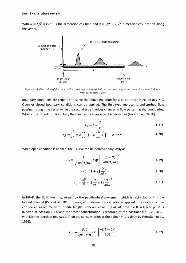
Part 1 - Literature review

78

With 𝜃 = 𝑡 𝑡⁄ = 𝑡𝑢 𝐿⁄ is the dimensionless time and 𝑧 = (𝑢𝑡 + 𝑥) 𝐿⁄ dimensionless location along

the vessel.

Figure 1.15- Illustration of the tracer pulse spreading due to axial dispersion according to the dispersion model (adapted from Levenspiel, 1999).

Boundary conditions are required to solve the above equation for a pulse tracer injection at z = 0.

Open or closed boundary conditions can be applied. The first type represents undisturbed flow

passing through the vessel while the second type involves changes in flow pattern at the boundaries.

When closed condition is applied, the mean and variance can be derived as (Levenspiel, 1999b):

𝑡�� = 𝑡 =

𝑉

𝜐 (1-27)

𝜎𝜃

2 =𝜎𝑡

2

𝑡2= 2(

𝐷

𝑢𝐿) − 2(

𝐷

𝑢𝐿)2

[1 − 𝑒−𝑢𝐿 𝐷⁄ ] (1-28)

When open condition is applied, the E curve can be derived analytically as:

𝐸𝜃 =

1

√4𝜋(𝐷 𝑢𝐿⁄ )exp [−

(1 − 𝜃)2

4𝜃(𝐷 𝑢𝐿⁄ )] (1-29)

𝑡�� 𝑡⁄ = 1 + 2 (

𝐷

𝑢𝐿) (1-30)

𝜎𝜃

2 =𝜎𝑡

2

𝑡2= 2

𝐷

𝑢𝐿+ 8(

𝐷

𝑢𝐿)2

(1-31)

In HRAP, the fluid flow is governed by the paddlewheel movement which is recirculating it in the

looped channel (Park et al., 2010). Hence, another method can also be applied : the reactor can be

considered as a tube with infinite length (Voncken et al., 1964). At time t = 0, a tracer pulse is

injected at position x = 0 and the tracer concentration is recorded at the positions x = L, 2L, 3L…jL

with L is the length of one cycle. Then the concentration at the point x = jL is given by (Voncken et al.,

1964):

𝐶𝑗𝐿 =

𝑄𝑗𝐿

2𝑗𝑉√𝜋𝐷𝑡𝑒𝑥𝑝 [

−(𝑗𝐿 − ��)2

4𝐷𝑡] (1-32)

Part 1 - Literature review

79

Where D is longitudinal dispersion coefficient, �� is the mean velocity and Q is the amount of tracer

and V is the volume of a section between x = jL and x = (j-1)L or the working volume of the HRAP.

As the fluid recirculated inside the channel, the sum of these concentrations recorded at the

positions x = L, 2L, 3L…jL will be:

𝐶 =

𝑄𝐿

2𝑉√𝜋𝐷𝑡∑𝑒𝑥𝑝 [

−(𝑗𝐿 − ��)2

4𝐷𝑡]

∞

𝑗=1

(1-33)

For completing one cycle, the fluid has to spend average 𝑡𝑐 = 𝐿 ��⁄ . Hence the dimensionless time is

𝜃 = 𝑡 𝑡𝑐⁄ . After a number of cycles, the tracer will finally be evenly distributed throughout the

reactor. The tracer concentration at infinite time will be 𝐶∞ = 𝑄 𝑉⁄ . The inverse of the vessel

dispersion number is uL D⁄ which is called the Bodenstein number or Bo (Voncken et al., 1964). The

previous equation can be rearranged as:

𝐶

𝐶∞= √

𝐵𝑜

4𝜋𝜃∑𝑒𝑥𝑝 [−

𝐵𝑜

4𝜃(𝑗 − 𝜃)2]

∞

𝑗=1

(1-34)

From this equation, the value of Bo and 𝜃 can be estimated by fitting the experimental data and used

to evaluate the mixing characteristics of the reactor (Voncken et al., 1964).

1.5.3 Virtual tracer experiments in CFD

There are two ways to perform a virtual tracer test in CFD. In the case of a steady-state flow, the flow

velocity field must first be calculated. Then, two options are available:

• Define a tracer (passive scalar) with the same properties as the flowing fluid, inject it at the

inlet through boundary conditions and follow the concentration of this pseudo compound at

the outlet. This method requires solving the transport of the tracer in transient conditions,

which can be computationally expensive;

• Define solid particles having the same density as the flow fluid and a very small diameter,

injecting a sufficiently large quantity to yield statistically significant results and observe the

time it takes for each particle to exit the system. The quantity of particles to be injected

depends on the precision that is required.

1.5.3.1 Scalar transport

The transport equations for a passive scalar are solved. The scalar (tracer) is injected by modifying for

a time step the tracer input concentration (by a modification of the boundary condition). In turbulent

flow, the transport equation is given by:

∂

∂t(ρC) + ∇ ⋅ (ρU C) = ∇ ⋅ ((ρ𝐷𝑚 +

μ𝑡

𝑆𝑐𝑡)∇𝐶)

Equation 1-35

Part 1 - Literature review

80

With Dm the molecular diffusion coefficient (m2/s), Sct the turbulent Schmidt number (non-

dimensional ratio). As it will be discussed later in the results concerning HRAP, this Sct parameter is of

fundamental importance (Chapter 4).

1.5.3.2 Lagrangian approach

In this approach, the residence time distribution can be deduced from the analysis of a large number

of particles trajectories in the reactor. The trajectory of a particle is predicted by integrating the

balance of forces applied to the particle in a Lagrangian reference frame (Fluent, 2005). The particles

are chosen with the same density as the continuous phase so that the gravitational forces are

neglected and only the drag force is to be considered. The turbulent dispersion of particles is taken

into account by a stochastic approach which considers that the particle interacts with a succession of

vortices generated by turbulence, the fluctuating velocities within the vortices are considered

isotropic and obey a Gaussian distribution.

1.5.3.3 Choice between the two methods

The particle tracking method is not affected by numerical dispersion. More information can be

extracted from it since the complete trajectory of each particle is obtained. The accuracy of the

simulation can be adjusted by choosing a larger or smaller number of particles.

Solving the transport equation of a tracer (passive scalar) allows more easily the assessment and

implementation of chemical or biological reaction models. In the case of HRAP, if one wants to access

to knowledge of algal cells trajectory and recurring exposure to light, the Lagrangian method is of

interest. If one wants to couple a biokinetic model, the transport equation of a tracer is relevant

because during the simulation, the chemical and biological reactions will be modeled by source/sink

terms in similar transport equations.

1.5.3.4 Dispersion modeling

The axial dispersion that is considered in the dispersion model can be considered as the sum of three

contributions at different scales: molecular diffusion, spatial dispersion and turbulent dispersion(Le

Moullec et al., 2008)

D  =  Dm  +  Ds   +  Dt

Equation 1-36

• Molecular diffusion (Dm): it is the macroscopic result of Brownian motion. This diffusion term

cannot be avoided but it is often considered as negligible in turbulent flows.

• Spatial (or kinematic) dispersion (Ds): when the model is 1D, spatial dispersion lumps

inhomogeneities of the flow field. These inhomogeneities may result among others from

edge effects, recirculation loops or preferential paths and dead zones.

• Turbulent dispersion (Dt): this is the result of the combined motion of all vortices generated

by turbulence.

Part 1 - Literature review

81

When computing the passive scalar transport Equation 1-35 in CFD, spatial dispersion is natively

considered due to the fact that the velocity field is calculated in 2D or 3D. There is therefore no

diffusion coefficient associated to it.

Turbulent dispersion: in the case of a turbulent flow, the turbulent transport of momentum and

concentration is stipulated in terms of turbulent (or eddy) viscosity and turbulent (or eddy)

diffusivity. The turbulent Schmidt number, Sct, is defined as the ratio of turbulent viscosity to

diffusivity (Donzis et al., 2014). The turbulent viscosity is computed by application of the RANS

approach for turbulence modeling (see section 1.3.2). As it will be discussed in section 1, this non-

dimensional number can have a great influence on the prediction of mass transport. However, in the

wastewater treatment field, most users use the default value provided by commercial software

packages such as FLUENT (recommended value of 0.7 for gas-liquid flows).

𝑆𝑐𝑡 =μ𝑡

𝐷𝑡

Equation 1-37

Numerical diffusion: in CFD, the numerical resolution and discretization of RANS and transport

equation can result in approximations errors due to e.g. spatial and temporal discretization schemes,

mesh quality (spatial discretization) and the time step (temporal discretization). This issue should be

considered when interpreting the results.

1.6 Conclusion and research questions

High rate algal pond (HRAP) is usually considered as a proper method for producing microalgae

biomass. It is the most widely used technique at both lab and commercial scale (Hadiyanto et al.,

2013; Hreiz et al., 2014b; Prussi et al., 2014). The main reason behind the broader acceptance of this

technique is its low operational cost and simplicity to build and operate the system (Prussi et al.,

2014). However, the hydrodynamics should be designed to ensure adequate mixing within the pond

for algal cells to grow and perform their photosynthetic activity efficiently. Some researchers doubt

the role of mixing in the productivity of algae since other factors such as temperature, light intensity,

liquid depth, CO2 and nutrient distribution have direct influence (Ali et al., 2015). Several other

experimental and numerical studies, on the other hand, shows proper mixing determines even

recurring light exposure of algal cell (Cheng et al., 2015; Liffman et al., 2013; Pruvost et al., 2006),

reduce settling and sedimentation of cells, and enable uniform distribution of nutrients and carbon

dioxide (Prussi et al., 2014; Richmond and Grobbelaar, 1986) in the culture while consuming

minimum possible energy to circulate the flow without damaging their mechanical structure

(Barbosa, et al., 2003).

This work is part of a research that intends to use wastewater as an algal culturing medium in HRAP

with an interest in comparing the hydrodynamic model results of two alternative approaches of CFD.

A first experimental study conducted in our lab to assess the impact of the operational condition on

oxygen transfer rate, mixing characteristics and residence time distribution using tap water has been

published before (Pham et al., 2018). The same operational conditions are also applied for

experimental and numerical investigation in this work.

Part 1 - Literature review

82

To perform virtual tracer tests using the CFD model, a scalar transport equation is coupled to the

flow governing equations. This equation accounts for advective transport and dispersion of tracer

material in the system. Dispersion depends highly on turbulence. Thanks to the turbulence model,

the turbulent dispersion term is computed by the ratio of turbulent viscosity to the turbulent

Schmidt number. This non-dimensional number value has to be carefully chosen to capture the

actual diffusivity in the system while not being a way to compensate for flaws in the CFD model. In

addition to illustrating the significance of paddle-wheel representation via Inlet Velocity and Dynamic

Mesh method in terms of accuracy and computational cost, this contribution aims to highlight the

impact of CFD model hypotheses (turbulence model) on the turbulent Schmidt number values that

can be estimated from the comparison between experimental and virtual tracer tests.

Part 2 - Materials and methods

83

2 Materials and methods

2.1 Pilot-scale Reactor Description

The lab-scale pond for the experimental work is designed and manufactured at ICUBE – Engineering

Science, Computer Science and Imaging Laboratory, Strasbourg, France. As discussed in section 1.2.2

of the previous chapter, the overall geometry of the pond and the paddlewheel need to be designed

as much efficient as possible to maximize production or aeration process at low cost. If the pond is

intended for algal fuel production, the total energy required for mixing must be below the energy to

be recovered from the biomass for economic viability. The purpose of this pilot is, however, to study

the detailed biochemical conditions, hydrodynamic properties, and their interdependencies. Hence,

the pond is designed to meet these objectives without being more concerned about the energy

input. Basic design features, such as depth, channel length to width ratio, minimum clearance of the

paddlewheel with side walls and maximum velocity for no damaging shear stress are however

considered.

A transparent ridged plastic material is used to construct the HRAP and the paddlewheel. The pond is

a single looped channel having a central length of 323cm, including the two 1800 curved ends and

two straight channels of width 20cm each (Figure 2.1). The central dividing wall is positioned in the

middle of the straight channel and the two deflectors are provided at midway in either side of the

two curves to smoothly guide the flow changing direction. Three shallow depths of flow, 10, 15 and

20cm, were assessed in terms of tracer tests and velocity profiles measurements. Hence, the total

height of the pond is decided to be 30cm with a freeboard of 10cm. The pilot reactor has a total

surface area of 0.633m2. As recommended by Hadiyanto et al., (2013), a high channel length to width

ratio of, 16 which is much above 10, is chosen to reduce dead zones. A 6 blades paddlewheel (73cm

in diameter) is installed inside one of the straight channels having minimum clearance with side walls

and channel bottom of 1.5cm and 2.5cm, respectively, to avoid backflow. It is run by a coupled

brushed DC motor (DMN37 K, 24 V, Nidec Servo Corporation, Japan) which is controlled by a bench

power supply (ISO-TECH IPS303DD, UK) (Figure 2.2).

2.2 Hydraulic Operational Conditions

In closed system conditions, different combinations of water level and paddlewheel rotational speed

were assessed. From the range of working depths reported by Muñoz and Guieysse, (2006), 3 water

levels of 10cm, 15cm, and 20cm were chosen with a total water volume of 72, 108 and 144 litres,

respectively. Three paddlewheel rotational speeds (Table 2.1) were employed for each depth of flow

by changing the voltage input to the motor from low mixing (3.5 Volt for 0.2±0.0A), to medium (7

Volt for 0.3±0.1A) and then to fast mixing (10.5 Volt for 0.6±0.1A). The average paddlewheel

rotational speed obtained were 12.5 ± 2.1, 11.2 ± 0.9 and 10.3 ± 0.4 rpm, respectively. The resulting

average flow velocities estimated from tracer experiment were 42.8cm/s for 10cm, 36.3cm/s for

15cm and 31.1cm/s for 20cm depth of flow. They are all higher than the recommended value of

30cm/s (Andersen, 2005a). Figure 2.3 shows that for the same voltage applied, the rotational speed

is decreasing as the depth of flow is increasing.

Of the nine depth and speed combinations, the three medium mixing conditions obtained from

applying 7 volts are used for detailed hydrodynamic simulation and tracer experiments.

Part 2 - Materials and methods

84

All the experiments were conducted indoor with ambient temperature of 20.9 ± 0.6oC and local air

pressure of 0.98 atm. Thus, both temperature and pressure are assumed to have no significant

impact on the measurements and calculations in this study. The basic physio-chemical properties of

the water used for the test were pH of 7.4 ± 0.1, conductivity of 557.7 ± 1.15μS/cm and temperature

of 15.1 ± 0.4oC. All these values were also assumed to be constant throughout the experiments.

Figure 2.1 - Schematic representation of the HRAP, (a) side view and (b) top view

(a)

Part 2 - Materials and methods

85

(b)

Figure 2.2 - Pictures of the HRAP, (a) running with tap water for flow velocity measurement and tracer test and (b) running partially treated wastewater for algal-bacterial biochemical study

Table 2.1 - Rotational speeds of the paddlewheel for the corresponding depth and applied voltage

Depth (cm) Rotational Speed (rpm)

(3.5Volt) (7Volt) (10.5Volt) 10 6.1 12.5 18.9 15 5.5 11.5 16.6 20 5.3 10.7 14.8

Figure 2.3 - Applied Voltage vs resulted rotational speed of the paddlewheel

2.3 ADV Measurements

A two-dimensional ultrasonic transducer is used to measure the flow velocity in the pilot HRAP. A

research group at the Mechanics Department of ICUBE Laboratory formerly named as Institute of

Fluid and Solid Mechanics of (Strasbourg, France), in collaboration with industrial partners and other

research institutions, has developed a versatile flowmeter: an ultrasonic device that can

simultaneously measure water flow and concentration of size classes of suspended particles (Abda et

0

5

10

15

20

3.5V 7V 10.5V

Ro

tati

on

al S

pee

d (

rpm

)

Applied Voltage

10cm 15cm 20cm

Part 2 - Materials and methods

86

al., 2009). This is achieved by the multi-frequency emitted by the device (1 to 14 MHz) that works

under the pulsed ultrasound principle to measure flow velocity, water height, and estimation of

suspended solids concentration. Velocity measurements rely on the Doppler principle.

Velocity at different points across the depth of the HRAP can thus be measured by using instruments

like this one that operate on the pulsed ultrasound principle (Figure 2.4) along the profile of the

backscattered beam (Abda et al., 2009). Such devices give accurate information about the position of

a given data at a given time step in the flow. An ultrasonic pulse is emitted into the medium at

appropriate interval. This signal is backscattered by the suspended particles in the flow and other

solid boundaries and received by the transducer. The backscattered signal received by the transducer

is conditioned, amplified and sampled in order to extract the information on the velocity and the

concentration of suspended solids. These values are estimated on a succession of measurement

volumes by windowing the backscattered signal in several blocs related to several measurement

depths. The device had been validated over long use of laboratory and field experiments and it

showed a very good agreement with other gauging methods. It is still in use for similar purposes

(François et al., 2016; Locatelli et al., 2015).

Figure 2.4 – Pulsed Ultrasound working principles showing echoes from particle and boundaries for consecutive pulsation (Abda et al., 2009)

For the velocity measurement in the lab HRAP, three sites were selected; before the end of the first

channel, the beginning of the second channel, and the end of the second channel (Figure 2.1). In

each site, three measurement points were chosen across the width of the channel: close to the outer

wall, the center of the channel and close to the middle separator.

The device used for this experiment consists of two sets of transducers. PORAVER particles, a type of

porous glass, having a size of 200 microns and a mean density close to 1g/cm3 are used as deflectors

of the beam emitted by the transducer. Two measurement sets were conducted: first, the transducer

is configured at 300 from the vertical to measure the horizontal flow velocity along the flow direction

and then it is aligned vertically to measure the vertical component of the flow. In all cases, the top of

the transducer needs to be immersed around 2cm below the free surface. Data is acquired for 150

seconds at every measuring step which is supposed to be enough to represent average flow profile.

To avoid the exaggerated eco from the transducer itself at the bottom of the channel, the first and

the last few time step records are omitted while interpreting the data. In total, 54 measurements

have been taken for all the three depths tested in two configurations, 27 for the inclined and 27 for

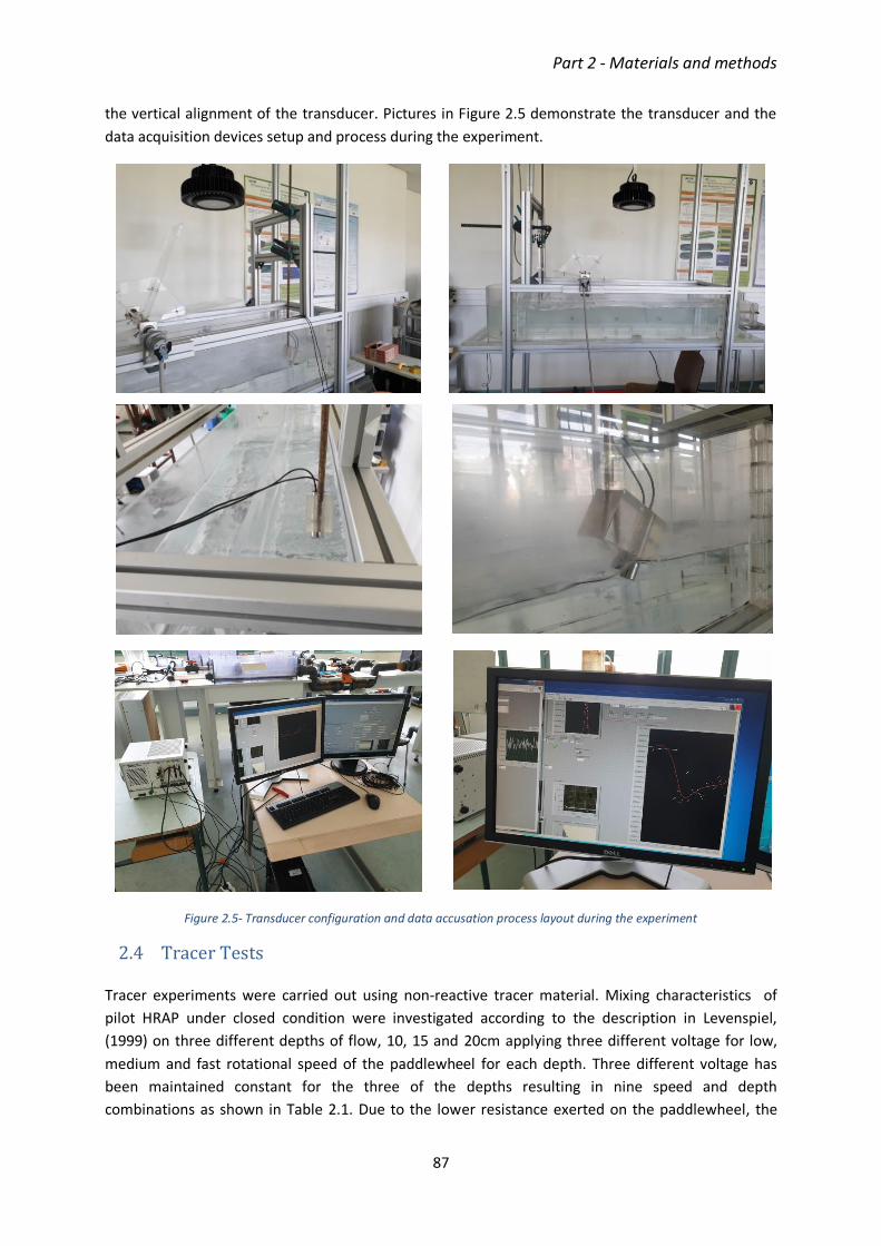
Part 2 - Materials and methods

87

the vertical alignment of the transducer. Pictures in Figure 2.5 demonstrate the transducer and the

data acquisition devices setup and process during the experiment.

Figure 2.5- Transducer configuration and data accusation process layout during the experiment

2.4 Tracer Tests

Tracer experiments were carried out using non-reactive tracer material. Mixing characteristics of

pilot HRAP under closed condition were investigated according to the description in Levenspiel,

(1999) on three different depths of flow, 10, 15 and 20cm applying three different voltage for low,

medium and fast rotational speed of the paddlewheel for each depth. Three different voltage has

been maintained constant for the three of the depths resulting in nine speed and depth

combinations as shown in Table 2.1. Due to the lower resistance exerted on the paddlewheel, the

Part 2 - Materials and methods

88

rotational speed is faster with lower depth. Consequently, as the depth increases, the rotational

speed decreases for constant voltage applied on the motor. For example, applying 7V on the 10cm

depth of flow resulted in a paddlewheel rotational speed of 12.5 rpm while the same voltage yielded

11.5rpm and 10.7rpm paddlewheel speed for 15 and 20cm depth of flow respectively.

Following a pulse injection of tracer (NaCl), water conductivity correlated with NaCl concentration

was measured by conductivity probe (TetraCon® 325, WTW, Germany) connected to a multi-

parameter portable meter (Multiline P4, WTW, Germany) and recorded with communications

software (Multi/Achat II, ver. 1.05, WTW, Germany). The probe is positioned at the center of the

channel around 50cm after the paddle wheel (Figure 2.1 and Figure 2.7).

Figure 2.6- Calibration curve for the correlations between NaCl concentration and conductivity in the water

In each test, depending on the water level (and as consequence, water volume) of the reactor,

different amounts of NaCl were used in order to maintain the conductivity level in the water at an

acceptable level for highest accuracy of the measurement. The total mass of NaCl used was 21.1,

31.6 and 42.2g for water level of 10, 15 and 20cm, respectively with a corresponding volume of 72,

108 and 144 liters. The NaCl used was stored at 105oC for 24h and then cooled in dry chamber before

the test to avoid atmospheric water absorption of the chemical. In order to improve the dissolution,

it was completely dissolved in 250 mL of tap water prior injection to the HRAP. The conductivity

measured in the water can be converted to the respective NaCl concentration using the calibration

line shown in Figure 2.6.

The HRAP was operated in closed condition (inlet and outlet flow rates were equal to 0). The

Voncken model (Mendoza et al. 2013) was used to compute Bodenstein number (Bo) and circulation

time (see section 1.5.2). These values then were used to assess mixing characteristics inside the

HRAP:

𝐶

𝐶∞

= √𝐵𝑜

4𝜋𝜃∑ 𝑒𝑥𝑝 [−

𝐵𝑜

4𝜃(𝑗 − 𝜃)2]

∞

𝑗=1

(2-1)

With C is the concentration of tracer detected, C∞ is the concentration of tracer at infinite time and θ

is the dimensionless time which is denoted as θ=t/tc (tc is circulation time and t is time).

Part 2 - Materials and methods

89

Figure 2.7 - Experimental setup for tracer test

2.5 Computational Fluid Dynamic Simulation Methods

In many other disciplines of fluid mechanics, particularly in the field of aeronautic engineering as it is

the birthplace of CFD (Anderson, 1995), due to finer experience and more precise fluid flow

requirements, CFD has established a standardized application guidelines (AIAA, 1998). Beyond the

hydrodynamic simulation of fluids, CFD has the potential to integrate with chemical and biological

unit process models for an optimum design and operation of wastewater treatment systems.

However, in addition to the need for powerful computing machine and storage device, and steep

learning curve of CFD, the lack of application methodologies had limited the use of CFD to the

analysis of hydraulic related problems only such as solid transport and sedimentation (Laurent et al.,

2014; Nopens et al., 2012). To extend its use, based on general CFD application procedures in other

areas and taking in to account the unique aspects of the wastewater engineering, an International

Water Association (IWA) working group, couple of years ago, has recommended a functional

modeling strategy (Wicklein et al., 2016). CFD model building in this study also primarily relied on this

guideline as shown in Figure 2.8.

Like other modeling procedures, CFD model building starts with defining the modeling objective and

deducing key assumptions based on the level of physics (number of phases and species involved,

fluids properties, thermal condition, state of the flow etc.), spatial dimensionality (2D or 3D), and

level of output accuracy required. For a complete representation of a system, CFD model may need

to be coupled with other models such as biochemical kinetics (conversion by reactions, growth rate

or decay), light irradiance model, and transport models (if additional materials are being transported

via the fluid). All these specific conditions dictate the modeling approach.

These tasks are followed by collecting the necessary information about the geometry and material

type of the processing equipment, and other pertinent documents including pictures and drawings.

Then the problem geometry is designed including the important physical details influencing the flow

and process being simulated using geometric modelling tools or should be imported from an existing

CAD drawing. There is always a trade-off between complexity and computational efficiency for the

modeller to decide. Small details, for instance, that do not significantly influence the bulk flow field

Part 2 - Materials and methods

90

and are of the order of, or significantly smaller than the computational mesh size are often neglected

(Wicklein et al., 2016).

Following the creation of the geometry, employing suitable tools, meshing or geometric

discretization can then be done to achieve appropriate type and size of mesh with an optimum

resolution level that fits well with the outlined geometry. Type and quality of the mesh critically

determines the stability and convergence of the calculation process. Unstructured meshes are more

flexible to fit closely within irregular geometries but structured types are numerically more stable.

Mesh with high degree of skewness and aspect ratio may ultimately cause the simulation to collapse

or result in diffusion errors. Moreover, convergence is assisted by introducing finer mesh gradation

at regions where the flow parameters are expected to make high variation that otherwise may

trigger numerical errors. Depending on the complexity of the geometry, meshing could be

challenging and tricky; hence, it must be carefully checked iteratively until an excellent mesh is

generated. Better fitting of highly refined mesh with the geometry enhance the representation of the

system and could give an improved result; but it would be at the cost of extended computational

time even for the mesh generation itself. Therefore, mesh independence check is required to verify

the solution and to ensure that it is not dependent upon the number and size of grids used to model

the given problem.

Part 2 - Materials and methods

91

Figure 2.8- Complete Flow ow CFD modelling processes. Source (Wicklein et al., 2016)

The steps described above are known as pre-processing. Success in these steps is vital to the next

stage of development which is the actual CFD model building. CFD models are used to solve the

governing equations of fluid flow or Navier–Stokes equations (section 1.3), which are based on

momentum balances with additional equations representing the turbulence characteristics of the

flow field. However, even the reduced versions of the conservation equations such as Reynolds-

averaged Navier-Stokes equation (section 1.3.2), have a non-closed nature due to the complex partial

differential elements. This compelled the solution, till the present day, to be completed only through

numerical methods by discretizing the flow domain in to a computational mesh to indicate the actual

location where the governing equation will be resolved. Finite Volume Method (FVM) is now

regarded as the most common discretizing method over Finite Element (FEM) and Finite Difference

Method (FDM) as it also allows the use of unstructured mesh.

Ridg2D/3D Phases

Steady/Unsteady Other

Geometry Photos

CAD/Shop Other

Material

Flows

CreateSupply

Type Size

Boundary Layers Software

Refinement

Aspect Skewness Other

Processor

PrecisionSolution

Output

Fluid/s

Boundary Turbulence UD

Convergence

Figure Animation

Field data Assumption

Tables Mesh

Key models

No

No

No

No

Yes

Yes

Geometry

Objective

Define Key Assumptions

Meshing

Mesh

Quality

Model Setup

Run Simulation

Post-processing, calibration and

Validation

Documentation Project

Data

Converge

d?

Mesh

Problem

?

Yes

Part 2 - Materials and methods

92

In general, model building stages includes setting the fluid properties, selecting suitable type of

turbulence model, defining boundary conditions, fixing solution methods and convergence criteria. It

is also at this level that the output is controlled directing to the predefined precision. Open and

flexible modeling packages allow users to formulate and introduce their own functions into the main

code whenever they need a specific task to simultaneously or subsequently be solved. Most of the

currently in use CFD models are compatible with parallel computing technology. Thus, the

computational domain can be optimally subdivided based on its total size and the available number

of processors for a reduced simulation time. However, partitioning should be done in the best

possible way not to take excessive reconstruction time. If the solution is not converged even after all

these deeds, rechecking of the mesh quality or the model setup criteria is necessary.

Otherwise, the solution is ready for interpretation, calibration and validation also known as post

processing. For the above model building steps performed in a satisfactory level, mostly boundary

conditions and mesh quality, the basic CFD model do not need calibration to solve the fundamental

fluid flow equations accurately for a single species/single phase as the parameters used are based on

the actual fluid flow phenomenon that are not uncertain (Wicklein et al., 2016). The case is slightly

different while applying CFD for wastewater modelling where uncertainties arises from the presence

of multiple phases and sub-models to represent the activities of scalar quantities within the flowing

fluid mass. Thus, CFD models essentially needs to be validated against a good quality experimental

data such as flow velocity, RTD, species concentration, temperature, shear stress, power

consumption and so on for a more reliable prediction. This particular study is focused on the use of

flow velocity and tracer data for validation and further analysis.

Final outputs of a validated CFD model can be presented in various methods. Figures and tables are

the common style to interpret the results and extract useful information from the simulation which

serves as an important input for design and analysis of a system under consideration. Most CFD

packages are either equipped with a post-processing tools or work seamlessly with other secondary

software to produce these figures and tables including the mesh used for the simulation, and

animations for better visualization. Under good modelling practice, new or unexpected results of CFD

model could reveal new insight and assist the modeler to infer accurate assumptions on the impact

of certain parameters on the fluid flow and mixing processes.

2.5.1 Description of the Methods and Assumptions

As mentioned at the beginning of this thesis, the objective of this work is to build a 3D model and

compare two alternative CFD approaches that could best represent the hydrodynamics inside the

lab-scale HRAP. One of the CFD modelling challenges, for a system having a rotating element in

general and for HRAP in particular, is the representation of the momentum induced by the rotating

paddlewheel that is usually in charge of inducing mixing and liquid velocity in such systems. Inlet

Velocity and Dynamic Mesh are the two common CFD techniques to simulate rotating elements

(Amini et al., 2016).

2.5.1.1 Inlet Velocity Method

Depending on the modelling objective, one can consider simplifying the simulation replacing the

paddlewheel by introducing a momentum source term in the governing equation or by assigning a

constant inlet velocity on a virtual inlet boundary (Hadiyanto et al., 2013). The later one is even

Part 2 - Materials and methods

93

easier to implement in OpenFOAM and it can also be used to model passive scalar transport of tracer

material by applying cyclic inlet and outlet boundaries. The rotational speed of the paddlewheel is

translated to an average horizontal velocity and uniformly imparted on the inlet boundary.

A small rectangular volume, in this case 1cm wide, is cut out of the flow depth exactly where the axis

of the paddlewheel lies. The two opposite faces of the cut along the flow direction, from the channel

to the cut volume and from the cut volume to the channel, would be outlet and inlet boundary,

respectively. Thus, the cyclic boundary condition continually transfers all flow information including

transported materials from outlet boundary to the inlet boundary until the simulation is ended

(Figure 2.9 a). Symmetrical boundary condition is given to the free surface of the liquid medium and

other solid surfaces; side walls, bottom of the reactor, middle separator and baffles are all given a

wall boundary condition. This method assumes a steady-state flow and therefore flow fields are

calculated from a steady-state condition.

2.5.1.2 Dynamic Mesh Method

Dynamic Mesh considers the rotation of the paddle-wheel geometry and simulates the momentum

transferred to the fluid through the rotating mesh (Hreiz et al., 2014b). In this method, linear motion

or rotation of a solid body, based on the physics of the problem under consideration, is handled by a

moving or rotating mesh with or without mesh morphing within the specified boundaries. However,

this approach could be computationally intensive (Ali et al., 2015) particularly when the model is

intended to be integrated with other models such as biokinetics, gas transfer, and light irradiance

models (Park and Li, 2015).

Paddlewheel is commonly installed and rotated with only a section of its impellers immersed into the

liquid at a time (Figure 2.9 b). The other parts turn above the free surface exposed to air until

immersed in the following cycle. Dynamic Mesh method realistically handle this phenomenon by

considering the top gas and the bottom liquid in which the paddlewheel intersects by implementing

the Volume of Fluid method (VOF) to determine the gas-liquid interface. Identical to the Inlet Velocity

method, other solid surfaces; side walls, bottom of the reactor, middle separator and baffles are all

given a wall boundary condition. In addition to the multiphase solver needed for the calculation, the

computational domain is increased due to the gas volume considered (

Figure 2.11). Transient solver is implemented in this method to account for the impellers position and

dependent mesh variables updating each time steps. Those precedents contributed the method to be

computationally demanding.

In Dynamic Mesh method, the rotation of the paddle-wheel is simulated using a boundary condition

called Cyclic Arbitrary Mesh Interface (cyclicAMI), a technique used to slide the moving mesh that

inscribed the paddlewheel against the adjacent static mesh domain of the same shape (Dellinger et

al., 2018). This is achieved by dividing the computational domain in two regions: rotating and stator

zones. The two regions are connected by two identical arbitrary meshing interfaces (AMI) at which

one slide over the other. A cylindrical shape rotating zone that fully circumscribes the paddlewheel

forms the first set which is the master AMI and the second or slave AMI covers the intersection area

with the stator. Thus, the paddlewheel rotational information is exchanged with the stator via these

two AMIs. As an advantage, except the reactor geometry and the paddlewheel’s rotational speed,

Part 2 - Materials and methods

94

this technique does not require prior knowledge of any of the flow characteristics (Hreiz et al.,

2014b).

Figure 2.9- (a) Inlet Velocity and (b) Dynamic Mesh schematics for the representation of HRAP

2.5.2 Geometric Design of HRAP

The real size of the pilot-scale HRAP is considered in the geometric design for both methods. In the

case of Inlet Velocity approach, since steady state is assumed, the exact depths of the liquid medium

(10, 15 and 20 cm) are used as height for the external wall, middle separator and flow deflectors. The

same height is also used for the inlet and outlet boundaries having a width equal to the width of the

channel. Actual thickness of the middle separating wall and deflectors are considered but thickness

of the external wall and bottom surface is not essential (

Figure 2.10).

To enclose the complete paddlewheel in the Dynamic Mesh technique, the geometry is modified by

raising section of the channel where the paddlewheel is found and the entire top surface is covered

by solid boundary to confine the gas phase so that atmospheric air is considered at the top as shown

in

Figure 2.11 and Figure 2.12. Moreover, freeboard is provided to accommodate the wave generated

by the rotation of the paddlewheel by increasing the heights of external wall, middle separator and

the flow deflectors above the respective flow depth. Walls thickness consideration is the same as

Inlet Velocity method. However, to reduce the computational load, the thickness of the propellers

and axis of rotation of the paddlewheel are neglected (

Figure 2.11 and Figure 2.12).

2.5.3 Meshing the Geometry

Two methods have been compared to design the geometry and generate a mesh for the lab-scale

HRAP. An open-source geometric designing and meshing tool, SALOME 8.5.3, was used first to create

and mesh the geometry for both the CFD modelling alternatives, Inlet Velocity and Dynamic Mesh

(Figure 2.10 and Figure 2.11). The final mesh information exported in UNV format is converted in to

OpenFOAM compatible format using an OpenFOAM converting utility, “ideasUnvToFoam”. The

Part 2 - Materials and methods

95

OpenFOAM package itself is also equipped with several versatile geometry and mesh generating

utilities that can vastly and satisfactorily design and mesh highly complex 2D and 3D shapes. In this

particular case, two of them, blockMesh and snappyHexMesh, are used for Inlet Velocity as well as

Dynamic Mesh approach (Figure 2.12).

The first option, SALOME, has a very good interactive graphical user interface (GUI) with sufficient

tutorials to learn and apply quickly. A helpful forum of user community is available for additional

support. Moreover, it is open-source and continuously upgrading currently to version 9.4.0.

However, creating and meshing complex geometries is a difficult process. Also meshing algorithms

are not so flexible and straight forward to control the process particularly for graded meshing.

blockMesh is a very powerful utility of OpenFOAM that creates parametric hexahedral meshes with

grading and curved edges (Greenshields, 2018). Block formation and mesh generation is directed by a

dictionary of code that explicitly gives the room to control each mesh parameters. The challenge in

using blockMesh is the absence of GUI which is common to all OpenFOAM solvers and utilities, a

slight difficulty in coding, limited to the generation of hexahedral blocks of mesh, and it is more

suitable to regular shapes only. Figure 2.13 demonstrates the section of the mesh generated by

blockMesh for Inlet Velocity method and Figure 2.14 demonstrates the piece of code used for this

mesh.

Figure 2.10- Geometry of HRAP (up) and layout with deflector and middle wall (bottom) for Inlet Velocity Method using SALOME

Part 2 - Materials and methods

96

Figure 2.11- Geometry of HRAP (up) and layout with baffles, middle wall and paddlewheel (bottom) for Dynamic Mesh Method using SALOME

Figure 2.12- Isometric view of HRAP geometry (a) blockMesh for Inlet Velocity, (b) snappyHexMesh for Dynamic Mesh method and (c) paddlewheel

The second OpenFOAM meshing tool used for the HRAP is snappyHexMesh that generates 3-

dimensional hexahedra and split-hexahedra meshes automatically from triangulated surface

geometries, or tri-surfaces, Stereolithography (STL) or Wavefront Object (OBJ) format (Greenshields,

2018). The mesh generation in snappyHexMesh is an iterative refining process of a base mesh and

morphing the resulting split-hexahedral mesh until the final mesh form approximately conforms to

the given surface. The background mesh is required to be slightly larger than the actual size of the

geometry to increase the chance of accurately snapping the surface. It can also shrink back the

resulting mesh and insert cell layers where treatment of a different function is needed. The

specification of mesh refinement level is very flexible, and the surface handling is robust with a pre-

specified final mesh quality. In each iteration, snappyHexMesh runs in parallel with a load balancing

Part 2 - Materials and methods

97

step (Greenshields, 2018). An automatic creation of the two AMI objects with the necessary numeric

features for the Dynamic Mesh method is only possible via snappyHexMesh.

Figure 2.13- Section of the mesh generated by blockMesh for Inlet Velocity method

Complex and irregular shapes can be meshed by snappyHexyMesh utility. But adjusting the multiple

parameters in the code is challenging. For an easy manipulation and quick visualization of

snappyHexMesh results, HELYX-OS graphical user interface is used in this study at the initial stage of

model development. HELYX-OS is an open-source GUI designed by ENGYS to work natively with the

standard OpenFOAM libraries. It provides an interactive, easy-to-use environment to perform all pre-

processing tasks in the CFD modelling including meshing but limited to a certain grid size. Otherwise

an enterprise version needs to be used.

Part 2 - Materials and methods

98

Figure 2.14- Script of the code used to generate the mesh via blockMesh

Part 2 - Materials and methods

99

Figure 2.15- Hexahedral Mesh generated by blockMesh and snappyHexMesh

2.5.3.1 Meshing for Inlet Velocity Approach

Unstructured mesh generated directly using SALOME is used for the Inlet Velocity method only.

However, steady state simulation of a single-phase flow was not converging and crashing after some

iteration (mesh quality was not sufficient). Simulation on structured mesh converged faster for nearly

the same number of cells. In addition to the obligatory use of snappyHexMesh to design the mesh for

the Dynamic Mesh method, as also stated above, blockMesh is more flexible and easier to control

mesh characteristics than SALOME. Due to these advantages, further simulations in this study were

conducted using a structured mesh generated via OpenFOAM utilities for Inlet Velocity method.

As shown in Figure 2.14, a dictionary “blockMeshDict” in the “system” directory of the CFD model

contains blocks of code to define the vertices of the shape, to control the edge type of the geometry

and mesh gradation in every direction. Each boundary is also defined with their respective type and

correct faces pattern. Due to the reasons stated at the beginning of this section, finer grading is used

for meshing closer to the middle and external wall, and at the both ends of the middle wall where

the flow made a sharp turn. Meshing starts from very fine level 482,963 for 10cm, 748,710 for 15cm

and 1,205,236 for 20cm) and was gradually made coarser until it has no influence on the simulation

result and converged in a fairly reasonable time. The final number of cells in the computational

domain and solution convergence time using intel ® core ™ i5 HP laptop having 8GB installed

memory and 2.4GHz CPU speed for the three depths tested in this study are presented in Table 2.2.

Checking the mesh quality in OpenFOAM (“checkMesh” utility): all cells are hexahedral, maximum

skewness, maximum aspect ratio, mesh non-orthogonality, and maximum cell openness are all

satisfactory.

Table 2.2 - Simulated flow depth, number of cell, convergence time, skewness and aspect ratio for Inlet Velocity method

Depth (cm) No.of hexahedral cell

Convergence time (s)

Maximum skewness

Maximum aspect ratio

20 417,100 1668 0.912 9.488

15 312,825 1506 0.972 9.489

10 208,550 1438 0.975 9.489

Part 2 - Materials and methods

100

2.5.3.2 Meshing for Dynamic Mesh Method

Due to the reasons stated above, structured mesh is only used in this method using snappyHexMesh.

Similar to “blockMeshDict”, a dictionary called “snappyHexMeshDict” in the system directory of the

general CFD model contains all the parameters to control the mesh characteristics. The

snappyHexMesh utility always needs a background or base mesh to produce the final mesh through a

step by step procedure. Two techniques, SALOME and blockMesh are tested to create this

background mesh.

All the geometric component of the HRAP is designed first in SALOME 8.5.3. Then, all surface

boundaries are meshed using a surface triangulation algorithm and exported in STL format. The

refinement level in SALOME is not decisive for the final mesh size as long as it creates a closed

surface to all boundaries. Those STL files are used in the snappyHexMeshDict to define the geometry.

However, probably due to the unstructured cells type at the two curved bends and intersection of

the middle wall and baffle with the bottom of the pond, snappyHexMesh didn’t create a closed

boundary surface at similar refinement level with blockMesh approach. Increasing the fineness leads

to an increase in the total cell size of the model that could result the need for huge computational

time.

The second alternative is to use blockMesh utility from OpenFOAM to define the background mesh.

Despite the longer lines of code, as stated in the above section, blockMesh provides better meshing

control and can help to design the exact shape of the HRAP with hexahedral cells only. The same

dictionary is extended to include the geometric modification in the Dynamic Mesh method. Since the

background mesh created in this way is exactly the same as the final geometry of the pond, it

simplifies the snappyHexMesh procedures. Improved smoothness and closed boundary surface has

been achieved in this method.

After the components geometry and the background mesh are properly defined, snappyHexMesh do

the meshing job in four steps. It begins with castellation of the background mesh based on the

problem geometry defined by the STL file. Criteria such as maximum global cell, number of cells

between different levels, rotating cell zones, regions of different refinement, resolve feature angles,

and so on can be set in the “castellatedMeshControls” sub-dictionary of the “snappyHexMeshDict”.

Castellation process is followed by snapping activity. The snapping phase attempts to adapt the

castellated mesh to conform to the input geometry. These controls are located in the

“snapControls” sub-dictionary. Snapping involves projecting and morphing the mesh to the surfaces

and features, in an iterative process. If the adaptations invalidate the mesh quality criteria, the step

is undone and replayed using modified parameters (Greenshields, 2018). The sequence ensures that

the resulting mesh achieves a minimum quality, at the expense of full geometry conformation. It is

recommended to adopt the dictionary file from a similar tutorial and to start with the default values

and adjusts them only after inspecting the mesh. The parameters need to be set for snapping onto

the surfaces and features separately (Greenshields, 2018).

In the third stage of the mesh generation process, according to the requirements in the

“addLayerControls” sub-dictionary such as expansion ratio, relative size, minimum thickness, feature

angle, and soon, prismatic cell layers are inserted into the voids formed by shrinking the mesh. These

Part 2 - Materials and methods

101

are constructed on boundary patches to make them smooth and closed. As final step, the

“meshQualityControls” sub-directory is used to specify the extreme values encountered during the

previous process to ensure that the resulting mesh is of sufficient quality for subsequent calculation.

The limits predominantly affect feature conformance, i.e. regions most likely to incur local mesh

distortion. If the mesh violates any of the limiting values, snappyHexMesh will attempt to re-apply

the offending changes with updated settings for additional cycles. This is an override of the mesh

quality settings when the “nRelaxedIter” has been reached (OpenCFD, 2011). The final adjusted

version of “snappyHexMeshDict” is annexed at the end of the thesis.

Mesh sensitivity in the case of Dynamic Mesh technique is mainly governed by the refinement level

of the propellers of the paddlewheel and the two AMIs. The propellers have diagonally aligned parts

even before the rotation starts at time zero. The intersection of these diagonal members with the

rest of the mesh domain creates highly skewed cells. As the cell size of the propellers mesh

decreases, the skewness of cells also goes down below the maximum limit. Similarly, the master and

the slave AMI must be sufficiently refined for nearly perfect edge and surface of their cylindrical

shape. This is essential because any roughness or mismatch between the two AMI’s edge and surface

would affect their smooth communication and cause the simulation to collapse. Dynamic Mesh

method is applied only to 20cm depth of flow because of huge computational time requirement.

Finer mesh was tested at the beginning with a cell size of 4,866,560. Without waiting for the

simulation to converge, the refinement level of the mesh is gradually reduced. And the final mesh

contains 1,036,720 cells of which 1,033,404 are hexahedral, 3,008 prisms and 308 polyhedral cells

with five faces. Maximum skewness and maximum aspect ratio are 3.725 and 14.079 respectively.

These values are clearly higher than the value of similar parameter of Inlet Velocity method. The

mesh is checked, and simulation smoothly runs with this quality. However, any further coarsening of

the mesh resulted in an immediate crashing of the simulation.

2.5.4 Solver Settings and Numerical Simulation

CFD simulation has been carried out using OpenFOAM 5.0 from the OpenFOAM Foundation for the

Inlet Velocity method. To take the advantage of constraining tracer element in one phase of a

multiphase flow, OpenFOAM-v1812 from ESI is used for the Dynamic Mesh method. In both cases, an

incompressible Newtonian fluid under isothermal condition is assumed.

2.5.4.1 Inlet Velocity

To execute flow field calculations of the steady-state conditions assumed in the Inlet Velocity

approach, “simpleFoam” solver is implemented. It is a steady-state solver for incompressible

turbulent flow using the SIMPLE (Semi-Implicit Method for Pressure Linked Equations) algorithm. This

algorithm is commonly used numerical procedures to solve Navier-Stokes equations in many CFD

applications (OpenCFD, 2011). Kinematic pressure and velocity are the two key initial inputs for the

solver to proceed the calculation. Initial conditions for both pressure and velocity are set based on

the physics of the HRAP (Table 2.3). The initial value on the “inlet” boundary is set by replacing the

moving zone boundary of the paddlewheel with the linear velocity calculated from the angular

velocity of the rotating paddlewheel by v= r*ω where v is the linear velocity (m/s) along the flow

Part 2 - Materials and methods

102

direction, r is the radius or the distance from the axis of the paddlewheel to the center of the flow

depth (m), and ω is the angular velocity of the rotating paddle wheel (rad/s).

Decomposition of the computational domain was not required in this case as a single core completed

the calculation in a fairly quick time. Time step has been set to one second with an end time of 2000

seconds. However, all the three simulations for the three depths converged before the end time

(Table 2.2).

Table 2.3- Boundary conditions for the Inlet Velocity approach

Inlet Outlet Free surface Walls

Pressure zeroGradient zeroGradient symmetry zeroGradient

Velocity fixedValue fixedValue symmetry fixedValue

nut calculated calculated symmetry nutkWallFunction

k fixedValue fixedValue symmetry kqRWallFunction

epsilon fixedValue fixedValue symmetry epsilonWallFunction

• zeroGradient: the quantity (here pressure) is developed in space and its gradient is equal to

zero in the orthogonal directions to the patch/boundary)

• fixedValue: this condition imposes a value at the patch for the given quantity (here velocity).

For walls, the value is set to 0 velocity (no-slip condition) whereas for inlet and outlet, it is

fixed according to the desired velocity.

• Symmetry: here, this condition is used to mimic the free surface when using the inlet velocity

method in single-phase simulation. It is analogous to a slip boundary condition.

• Wall functions: the boundary conditions for k, and turbulent viscosity are the standard one

supplied by OpenFOAM. For more details on their implementation, the reader can refer to

(Liu, 2016).

2.5.4.2 Dynamic Mesh

Due to the presence of air at the top, a multiphase solver “interDyMFoam” is required for this case. It

is a transient solver for 2 incompressible, isothermal immiscible fluids with optional mesh motion

and mesh morphing including adaptive re-meshing (OpenCFD, 2011). It is using PIMPLE algorithm

that combines SIMPLE and PISO (pressure-implicit split-operator) algorithms. The solver implements

the Volume of Fluid (VOF) phase fraction interface capturing method to define the free surface

(Devolder et al., 2015) (section 1.3.3).

The pressure inside the closed HRAP is assumed to be atmospheric and thus except the two AMIs all

other boundaries are initially assigned with this fixed flux of pressure with zero gradient. The internal

field velocity value is also zero at the start. The angular speed of the rotating zone in rad/s with its

origin and direction of the axis of rotation is defined in a specific dictionary called

“dynamicMeshDict”. It is in this same dictionary that the mesh deformation and mesh morphing are

Part 2 - Materials and methods

103

controlled. In fact, this dictionary is one of the less standardized features of OpenFOAM: different

versions have different mechanisms to handle the representation of mesh motion or rotation and

mesh morphing. The version used for this study has four method of capturing these phenomena. The

two marginal cases are static mesh or no mesh motion condition “staticFvMesh”, and mesh motion

based on solved mesh motion for rigid body motion “dynamicMotionSolverFvMesh”. Even though it

is computationally intensive, the last option is more appropriate to handle mesh motion associated

with rotating solid boundary. Hence, this option is adopted in this study (Figure 2.16).

Similar to the previous method, the turbulence characteristic of the flow is simulated using the k-

epsilon RAS model and the turbulence parameters are calculated from the known flow values as

illustrated in the Equation 2-6 and Equation 2-7 below. Basic fluid properties (density, viscosity, and

surface tension) of both phases are considered at room temperature (20°C) and pressure (0.98atm).

The solver, “interDyMFoam”, needs additional dictionary “setFieldDict” to determine the regions of

the two phases at the start of the simulation. Depending on the actual shape of the phase volume,

the dictionary helps to define their respective regions using different techniques, box to cell, sphere

to cell, etc. The “setField” utility is then executed to set the value of each phase to the specified

regions overriding the default field values. This utility is also used to define the passive scalar tracer

element inside the liquid zone. Therefore, “boxToCell” is used for the bottom liquid and

“sphereToCell” is applied for the virtual tracer material (see section 2.5.5). The default value is for the

gas phase (Figure 2.17).

Figure 2.16 Mesh motion type specified in the dictionary “dynamicMeshDict” with the origin of rotational axis and rotational speed

Part 2 - Materials and methods

104

Table 2.4 - Boundary conditions for Dynamic Mesh method

Field AMI-1 AMI-2 paddlewheel Walls

Pressure cyclicAMI cyclicAMI fixedFluxPressure fixedFluxPressure

Velocity cyclicAMI cyclicAMI movingWallVelocity fixedValue

nut cyclicAMI cyclicAMI nutkWallFunction nutkWallFunction

k cyclicAMI cyclicAMI kqRWallFunction kqRWallFunction

epsilon cyclicAMI cyclicAMI epsilonWallFunction epsilonWallFunction

alpha.water cyclicAMI cyclicAMI zeroGradient zeroGradient

A cyclicAMI cyclicAMI zeroGradient zeroGradient

Boundary conditions for paddlewheel and walls are no-slip for velocity. For turbulence, standard wall

functions are used. Specification of boundary conditions for turbulence requires additional

calculations. Hydraulic Diameter (DH) and Reynolds Number (Re) are calculated as:

𝐷𝐻 = 4𝐴

𝑃

Equation 2-2

𝑅𝑒 =𝐷𝐻 × 𝑉 × 𝜌

𝜇

Equation 2-3

Where A and P are the wetted area and wetted perimeter respectively, V is the average flow velocity,

ρ and μ are the density and dynamic viscosity of the liquid.

Assuming a fully developed pipe flow, turbulent length scale (l) and turbulent intensity (I) are also

calculated as below.

𝑙 = 0.038 × 𝐷𝐻

Equation 2-4

𝐼 =0.16

𝑅𝑒𝐷𝐻

18⁄

Equation 2-5

ReDH is the Reynolds number calculated based on the hydraulic diameter. The calculated values DH,

Re, l and I are 0.262m, 81,295.61, 0.00996 and 0.0389 respectively. Based on these values the

turbulent parameters for the k-epsilon model are estimated as shown below.

𝑘 = 1.5(𝑉 × 𝐼)2

Part 2 - Materials and methods

105

Equation 2-6

∈=𝐶𝜇𝐾1.5

𝑙

Equation 2-7

Where k is the turbulent kinetic energy, ε is the rate of dissipation of turbulent kinetic energy and Cμ

is a model constant which in the standard version of the k-epsilon model has a value of 0.09.

To observe main details of evolution of fluid flow, time step is crucial in accurate transient

simulation. Criteria to set the time step varies depending on the type of solver implemented. Courant

number, based on the stability analysis of inertial effect, is generally enough for most solvers. In

addition to this, while applying Dynamic Mesh method, to avoid end of the simulation due to a very

tiny mismatch between the two cyclic AMI’s, adjustable time step is set so that the solver accordingly

modifies it.

For the final grid size of 1,036,720 cells, decomposing the total computational domain into optimum

number of subdomains was necessary to perform parallel calculation on the High-Performance

Cluster (HPC) computing system of the University of Strasbourg. Three dividing options (16, 32 and

64 processors) have been tested. The first and the last (16 and 64 processors) were slower than 32

processors probably due to bigger computational demand for 16 processors and large reconstruction

time for the 64 processors.

Figure 2.17- Initial phase volume fractions of HRAP

2.5.5 Tracer Transport

2.5.5.1 Inlet Velocity

In the Inlet Velocity method, for simulating scalar transport of the pulse tracer injection, an

equivalent spherical volume of numerical tracer element is introduced at the center of flow depth

exactly where the actual tracer experiment used to inject the sodium chloride solution (Figure 2.1).

As mentioned in the above section, “setField” utility is used to set the virtual tracer at the intended

location inside the computational domain. To ensure swapping of the transported tracer material

from the outlet face back to the inlet face, Cyclic boundary condition is applied.

Part 2 - Materials and methods

106

Tracer transport is represented by the passive scalar transport equation. Using the finally converged

solutions of flow field quantities from “simpleFoam” solver, “scalarTransportFoam” solver in

OpenFOAM is implemented to solve this transport equation separately. However, the original solver

didn’t consider the turbulence effect in dispersion/mixing to solve the equation for the scalar

transport of tracer material. Due to this reason the equation is modified by adding a ratio of

turbulent viscosity (μt) over turbulent Schmidt Number (Sc) to the molecular diffusion coefficient. As

depicted above, the turbulent viscosity is calculated from the known flow parameters. The default

Schmidt Number value (0.7) was used as an initial guess and two iterations were made by reducing

the value up to 0.35.

𝜕

𝜕𝑡(𝜌𝐶) + ∇. (𝜌�� 𝐶) = ∇. ((𝜌𝐷𝑚 +

𝜇𝑡

𝑆𝑐𝑡)∇𝐶)

Equation 2-8

where C represents the concentration of tracer, U the water velocity, ρ the water density, Dm the

molecular diffusion coefficient (1.9.10-9 m2/s), µt the eddy viscosity, Sct the turbulent Schmidt

number.

2.5.5.2 Dynamic Mesh

The injection location and method is the same with the Inlet Velocity approach. And the same

transport equation is solved in the Dynamic Mesh method. However, since “interDyMFoam” is a

transient solver, “scalarTransportFoam” need to be resolved simultaneously. Different OpenFOAM

versions provide a system to implement “scalarTransportFoam” onto other solvers as a function

object. This technique was first used in OpenFOAM 5.0 but the result was not in line with the actual

physics of the HRAP. As described in section 2.4, sodium chloride solution, which is obviously not

volatile, was used as a tracer material. In the real experiment, this solution is only diffused in the

liquid medium. Contrary to this reality, numerical as well as graphical result from OpenFOAM 5.0

shows some amount of tracer go beyond the liquid zone and distributed in the gas region considered

for Dynamic Mesh (Figure 2.18). This is means that the solver didn’t constrain the tracer in the liquid

phase only. Since OpenFOAM-v1812 has this capability, it is preferred for this case.

Figure 2.18- Diffusion of tracer material in the gas phase

Part 3 - Experimental Hydrodynamic Characterization of the HRAP

107

3 Experimental Hydrodynamic Characterization of the HRAP

Two sets of experimental studies, velocity measurement and tracer tests, were conducted on the lab

scale HRAP to see how the hydrodynamics inside the pond is behaving. The data collected in the

experimental work are very essential for the CFD model validation. The following sections present

the summarized results.

3.1 Velocity measurement using ADV instrument

Velocity measurement on the lab scale HRAP has been carried out using an ultrasonic transducer

ADV meter. The instrument was developed and calibrated at the ICUBE laboratory as described in

section 2.3. Detailed specification of the instrument is presented in Table 3.1.

The device can measure two-dimensional velocity profiles and hence the two predominant velocity

components, along the flow directions and in the vertical direction, were gauged. The flow along the

width of the channel is assumed to have a small magnitude and not considered in the measurement

campaign. Measurement is performed on clear tap water before algae was introduced and fine sand

particles are used to serve as suspended solids to reflect the ultrasonic signal emitted by the

transducer.

Three measuring sites were selected; before the end of the first channel, the beginning of the second

channel, and the end of the second channel (Figure 2.1). In each site, three measurements were

taken across the width of the channel; 1.5cm from the outer wall, at the center of the channel and

1.5cm from the middle separator wall. The device used for this experiment consists of two sets of

transducers and data from each set is separately recorded and averaged. Two measurement

configurations were conducted at each site and location. First, the transducer is oriented in 30° angle

from the vertical to measure the horizontal flow velocity along the flow direction and then it is

aligned vertically to measure the vertical component of the flow. In all cases, the device is kept 2cm

below the free surface of the water for around 2 minutes.

Velocity measurement is conducted for the three operating depths (10, 15, and 20) cm as described

in the hydraulic operational conditions of the HRAP (section 2.2). In total, 54 measurements were

taken from the three sites for the three depths tested.

Part 3 - Experimental Hydrodynamic Characterization of the HRAP

108

Table 3.1- Description of the Ultrasonic Transducer used in the HRAP

Items Value

Sensor Diameter 2cm

Maximum Pulse Repetition Frequencye f f * 4000 Hz

Maximum measurable velocity 3 m/s

Central frequency 2 MHz

Carrier frequency 2 MHz

Spatial Resolution 0.5 cm

Time Resolution 1s

3.1.1 Horizontal Velocity

Measured velocity profiles from the three sites are selected and presented in the following graphs.

Figure 3.1 shows the orientation of the axes with respect to the flow direction. Hence, horizontal

component refers to the velocity in the flow direction or y-axis which has positive value in the first

channel and negative when the flow is returning after the curve in the second channel. Flow velocity

in the x-axis which is perpendicular to the flow direction in the same horizontal plane is assumed to

have small magnitude and hence neglected. Vertical velocity component is along the z-direction.

Figure 3.1- Orientation of axes with respect to flow direction

Part 3 - Experimental Hydrodynamic Characterization of the HRAP

109

3.1.1.1 First Measuring Site

(a)

(b)

Arthmetic and trigonometric processing is required before interpreting the raw data collected from

the meter. Average of the two ADV probes which are aligned in the same orientation during all the

measurments, is first calculated before proceding with the trignometric operation. Since the ADV

probe is aligned 300 from the vertical, the horizontal component is calculated as the sin component

Figure 3.2- Horizontal Velocity Profile (first sensor) at the first measuring site 1.5cm from the outer wall for 10cm depth of flow (a) before post-processing (b) after post-processing

Part 3 - Experimental Hydrodynamic Characterization of the HRAP

110

of the average flow. Figure 3.2(a) shows the total processed horizontal velocity profile from the

transducer plotted againest the depth of the liquid. This measurement is conducted on the 10cm

depth of flow. However, nearly 10cm below the free surface the velocity starts to increase or diverge

again. This is due to the echo from the bottom surface and underneeth air. Hence, it should be

clipped accordingly as shown in Figure 3.2(b). Similarly, due to the stronger wave at the free surface

and the interface with atmospheric air, few records of the instrument at the top 1 or 2cm have

uncharacteristical values and therefore they are trimmed off from the result. Measurments on other

sections and depths presented henceforth are subjected to a similar postprocessing procedure.

(a) (b)

Figure 3.4- Horizontal Velocity Profile (average of the two sensors) at the first measuring site 1.5cm from the outer wall for 10cm depth of flow

Figure 3.3- Horizontal Velocity Profile (second sensor) at the first measuring site 1.5cm from the outer wall (10cm depth of flow)

Part 3 - Experimental Hydrodynamic Characterization of the HRAP

111

(a) (b)

(a) (b)

Figure 3.5- Horizontal Velocity Profile (average of the two sensors) at the first measuring site at the centre of the channel (a) 10cm and (b) 20cm depth of flow

Figure 3.7- Average Horizontal Velocity Profile at the first measuring site (Average of the three measuring points) 10cm depth of flow

Figure 3.6- Horizontal Velocity Profile (average of the two sensors) at the first measuring site 1.5cm from the middle wall (a) 10cm (b) 20cm depth of flow

Part 3 - Experimental Hydrodynamic Characterization of the HRAP

112

In the experimental results presented above, despite the slight variation in magnitude, the measured

horizontal velocity profile from the three measuring points at the first site is having a similar pattern

(Figure 3.4, Figure 3.5 and Figure 3.6). Theoretically the maximum velocity is expected to coincide

with the center of the channel. However, in the case of 10cm depth of flow, the maximum horizontal

velocity (75.7cm/s) was gauged at the third measuring point (close to the middle wall) at around

6.32cm above the bottom surface or 2.68cm below the free surface. As will be discussed in the next

chapter, the numerical result also shows the maximum horizontal velocity is shifted from the center

towards the middle wall of the HRAP. This was not the case for the 20cm depth of flow where the

maximum velocity has been recorded at the center of the channel (98.3cm/s) at around 16.2cm

above the bottom surface or 2.8cm below the free surface. The overall average velocity over the

entire section of the channel is 57.4cm/s for 10cm and 51.2cm/s for 20cm depth of flow.

3.1.1.2 Second Measuring Site

(a) (b)

Figure 3.8- Average Horizontal Velocity Profile at the first measuring site (Average of the three measuring points) 20cm depth of flow

Figure 3.9- Horizontal Velocity Profile (average of the two sensors) at the second measuring site 1.5cm from the middle wall (a)10cm (b)20cm depth of flow

Part 3 - Experimental Hydrodynamic Characterization of the HRAP

113

(a) (b)

(a) (b)

Figure 3.10- Horizontal Velocity Profile (average of the two sensors) at the second measuring site at the center of the channel (a)10cm (b)20cm depth of flow

Figure 3.11- Horizontal Velocity Profile (average of the two sensors) at the second measuring site 1.5cm from the outer wall (a)10cm (b)20cm depth of flow

Figure 3.12- Average Horizontal Velocity Profile at the second measuring site (Average of the three measuring points) (10cm depth of flow)

Part 3 - Experimental Hydrodynamic Characterization of the HRAP

114

The second measuring site is again on the straight channel 15cm after the end of the first bend

(Figure 2.1). Due to the sharp bend around the middle separator wall, the flow is expected to be

separated from the boundary or form a dead zone. This phenomenon caused the velocity at around

the center of the depth to be significantly reduced or change its direction. At this measuring location,

recirculation has occurred as observed in Figure 3.9 and Figure 3.10. Because of this recirculation,

two visible velocity picks are seen in this section as plotted on the same graphs. This phenomenon is

very similar for both depths presented here. As the measuring point goes away from the middle

separator wall towards the outer wall, the flow pattern is changed back more like normal open

channel flow profile as shown in the third measuring point of the second measuring site (Figure

3.11). However, the velocity profile at this point (close to the outer wall) is not yet fully a normal

open channel flow distribution with the maximum velocity shifted downward, probably due to the

adjacent vortex.

3.1.1.3 Third Measuring Site

(a) (b)

Figure 3.13- Average Horizontal Velocity Profile at the second measuring site (Average of the three measuring points) (20cm depth of flow)

Figure 3.14- Horizontal Velocity Profile (average of the two sensors) at the third measuring site 1.5cm from the middle wall (a)10cm (b)20cm depth of flow

Part 3 - Experimental Hydrodynamic Characterization of the HRAP

115

(a) (b)

(a) (b)

Figure 3.15- Horizontal Velocity Profile (average of the two sensors) at the third measuring site at the center of the channel (a)10cm (b)20cm depth of flow

Figure 3.16- Horizontal Velocity Profile (average of the two sensors) at the third measuring site 1.5cm from the outer wall (a)10cm (b)20cm depth of flow

Part 3 - Experimental Hydrodynamic Characterization of the HRAP

116

Figure 3.18- Average Horizontal Velocity Profile at the third measuring site (Average of the three measuring points) (20cm depth of flow)

The third measuring site is on the second channel 10cm before the flow enters the second curve

(Figure 2.1). The flow in this location is supposed to have a normal open channel flow character with

a theoretical maximum velocity at 2/3 of the depth from the bottom or 1/3 of the depth from the

free surface. The plotted velocity profile for both cases presented, 10cm and 20cm depth of flow is

very close to this theoretical fact. For 10cm flow, however, the maximum velocity is slightly shifted

downward toward the center of the depth that looks like a flow profile in a pipe flow. This could

probably be since this location is far from the momentum source or paddlewheel in which the

velocity is lower than upstream sites and the shear resistance is propagated from the bottom surface

on a shallow depth of flow.

3.1.2 Vertical Velocity

3.1.2.1 First Measuring Site

Similar procedure is applied on the same transducers configured vertically to measure velocity

component in the z-direction. The same post-processing technique is also considered for readings

below the bottom surface of the HRAP.

(a) (b)

Figure 3.17- Average Horizontal Velocity Profile at the third measuring site (Average of the three measuring points) (10cm depth of flow)

Figure 3.19- Vertical Velocity Profile at the first measuring site 1.5cm from the outer wall for 10cm depth of flow (a) first sensor (b) second sensor

Part 3 - Experimental Hydrodynamic Characterization of the HRAP

117

(a) (b)

(a) (b)

(a) (b)

Figure 3.21- Vertical Velocity Profile (average of the two sensors) at the first measuring site at the center of the channel (a) 10cm (b) 20cm depth of flow

Figure 3.20- Vertical Velocity Profile (average of the two sensors) at the first measuring site 1.5cm from the outer wall (a)10cm (b) 20cm depth of flow

Figure 3.22- Vertical Velocity Profile (average of the two sensors) at the first measuring site 1.5cm from the middle wall (a) 10cm (b) 20cm depth of flow

Part 3 - Experimental Hydrodynamic Characterization of the HRAP

118

3.1.2.2 Second Measuring Site

(a) (b)

Figure 3.23- Average Vertical Velocity Profile at the first measuring site (Average of the three measuring points) (10cm depth of flow)

Figure 3.24- Average Vertical Velocity Profile at the first measuring site (Average of the three measuring points) (20cm depth of flow)

Figure 3.25- Vertical Velocity Profile (average of the two sensors) at the second measuring site 1.5cm from the middle wall (a)10cm (b)20cm depth of flow

Part 3 - Experimental Hydrodynamic Characterization of the HRAP

119

(a) (b)

(a) (b)

Figure 3.26- Vertical Velocity Profile (average of the two sensors) at the second measuring site at the center of the channel (a)10cm (b)20cm depth of flow

Figure 3.28- Average Vertical Velocity Profile at the second measuring site (Average of the three measuring points) (10cm depth of flow)

Figure 3.27- Vertical Velocity Profile (average of the two sensors) at the second measuring site 1.5cm from the outer wall (a)10cm (b)20cm depth of flow

Part 3 - Experimental Hydrodynamic Characterization of the HRAP

120

3.1.2.3 Third Measuring Site

(a) (b)

(a) (b)

Figure 3.29- Average Vertical Velocity Profile at the second measuring site (Average of the three measuring points) (20cm depth of flow)

Figure 3.30- Vertical Velocity Profile (average of the two sensors) at the third measuring site 1.5cm from the middle wall (a)10cm (b)20cm depth of flow

Figure 3.31- Vertical Velocity Profile (average of the two sensors) at the third measuring site at the center of the channel(a)10cm (b)20cm depth of flow

Part 3 - Experimental Hydrodynamic Characterization of the HRAP

121

(a) (b)

Figure 3.32- Vertical Velocity Profile (average of the two sensors) at the third measuring site 1.5cm from the middle wall (a)10cm (b)20cm depth of flow

Figure 3.33- Average Vertical Velocity Profile at the third measuring site (Average of the three measuring points) (10cm depth of flow)

Figure 3.34- Average Vertical Velocity Profile at the third measuring site (Average of the three measuring points) (20cm depth of flow)

Part 3 - Experimental Hydrodynamic Characterization of the HRAP

122

Table 3.2- Summary of the measured velocity values

Depth Measuring site

Horizontal Velocity(cm/s) Vertical Velocity(cm/s) Point 1 Point 2 Point 3 Average Point 1 Point 2 Point 3 Average

10cm 1 45.2 54.1 62.6 53.9 15.8 4.8 37.0 19.2

2 25.2 57.5 86.9 56.5 2.9 -22.4 17.8 -0.5

3 62.9 71.3 80.3 71.5 16.8 10.4 7.8 11.6

60.6 10.1

15cm 1 51.87 53.18 57.06 54.04 18.01 0.83 33.4 17.41

2 25.94 87.77 86.41 66.71 11.3 -11.1 34.7 11.63

3 67.19 71.51 69.84 69.51 11.9 15.1 18.16 15.05

63.42 14.69

20cm 1 47.2 55.3 51.2 51.2 16.7 2.1 33.1 17.3

2 32.3 71.5 82.9 62.2 -0.5 -21.9 44.0 7.3

3 65.9 68.9 59.1 64.6 -2.3 8.8 17.5 8.0

59.3 10.8

As observed on the horizontal velocity profile graphs, the general trend of vertical velocity pattern

for the 10cm and 20cm depth of flow are very similar in all the three sites in three of the measuring

points (Figure 3.19 - Figure 3.32). Vertical velocity components at the first measuring site of first

measuring point (1.5cm from the outer wall) are mainly having positive value with a maximum

velocity of 48.1cm/s for 10cm and 50.1cm/s for 20cm depth of flow, both observed close to the free

surface (Figure 3.19). At this point, few negative vertical velocities are observed around the bottom

surface of the pond.

The vertical velocity profile at the second site supports the argument discussed in section 3.1.1. In

the second measuring site at the second measuring point (at the center of the channel), significant

negative vertical velocities are recorded around the mid depth of the flow. This shows the existence

of recirculation in the vertical direction (Figure 3.21) at both depths. The third measuring point shows

similar velocity pattern with the first one (Figure 3.22). The average vertical velocity profile of the

three measuring points are shown in Figure 3.23 for 10cm depth and Figure 3.24 for 20cm. The

average vertical velocity over the entire section of the channel at this site are 19.2cm/s and 17.3cm/s

which are significantly smaller than the horizontal component 57.4cm/s and 51.2cm/s for 10cm and

20cm depth of flow respectively. Very similar velocity profiles are observed in the other two sites

(Figure 3.25 - Figure 3.34).

3.2 Tracer tests

Tracer tests using NaCl as a tracer material were performed in different conditions to assess the

mixing inside the HRAP. The parameters (circulation time tc and Bodenstein number Bo) derived from

Voncken et al., (1964) model were identified by minimizing the sum of squared error between

experimental data and model predictions (solver add-in in Microsoft Excel).

Following equation (2-1), at time t, the ratio between tracer concentration recorded at the sensor’s

position C and the final concentration (infinite concentration at well mixed) Cinfinite can be obtained.

As indicated by Miller and Buhr, (1981), non-ideality of the input pulse is expected in such test

resulting to imperfect record of the first and in some cases, the second peak. Hence the priority of

fitting was focused on the third peak onwards (Miller and Buhr, 1981). The fitting curves from mixing

Part 3 - Experimental Hydrodynamic Characterization of the HRAP

123

characteristics tests in this study are presented below for the different water depths and

paddlewheel rotation speeds investigated:

(a)

(b)

(c)

10cm_12.5rpm

10cm_18.9rpm

10cm_6.1rpm

Part 3 - Experimental Hydrodynamic Characterization of the HRAP

124

(d)

(e)

(f)

15cm_5.5rpm

15cm_11.5rpm

15cm_16.6rpm

Part 3 - Experimental Hydrodynamic Characterization of the HRAP

125

(g)

(h)

(i)

Figure 3.35 - Fitting curves (Voncken model vs. real data) for each mixing characteristics test

20cm_10.7rpm

20cm_5.3rpm

20cm_14.8rpm

Part 3 - Experimental Hydrodynamic Characterization of the HRAP

126

The Voncken model allows to estimate the respective values of Bodenstein number (Bo) and

circulation time. The Bodenstein (Bo) quantifies the ratio between total momentum and longitudinal

dispersion to solute transport within the system (Voncken et al., 1964).

The high values of Bo for every experiments (around 100) suggest plug flow behaviour in the pilot

HRAP, which is in accordance with the literature ( El Ouarghi et al., 2000). For all the water depths,

Bo increased with paddle rotational speed (Figure 3.36b). Higher rotational speed induced an

increased velocity in the direction of the rotation (y-axis) and thus a higher advective transport of the

tracer (Figure 3.36c). At the same time, for a given rotational speed, Bo decreased with an increase in

the water depth, meaning that dispersion increased when water depth increased: one could expect

water velocity to significantly change with water depth but as highlighted in the previous section,

velocity profiles displayed similar order of magnitude. The main reason explaining this higher

dispersion is that, with more water, the paddlewheel is more immerged and induce vertical mixing

on a higher water column. It also yields probably more turbulent dispersion in these conditions.

In general, tracer curves can be used to estimate the mixing time inside a reactor. Mixing time is

known to be highly influenced by the

hydrodynamic condition. The

higher the turbulence of a flow

due to increased momentum source

or presence of stirring device such

as paddlewheel, the smaller the mixing

time would be while laminar or layered flows are characterized by excessive mixing time. Table 3.3 is

showing the approximate mixing time for the three depths for three different paddlewheel rotational

speeds. As shown in Figure 3.36 (a) and (c), the effect of increasing the rotational speed of the

paddlewheel is in general reduce the circulation time and increase the average flow velocity.

However, the depth of flow does not affect circulation time and average velocity.

From the circulation time and knowing the pilot reactor geometry, the average water velocity along

the channel was calculated (Figure 3.36c,

Table 3.4). Literature suggests that water velocity of 0.2 to 0.3 m/s is enough for algal culturing in

HRAP. This condition was satisfied even with the lowest rotational speed (5.6 rpm). The highest

speed (16.8 rpm), although improving mixing in the pond, could yield higher shear stress on algal

cells and more energy consumption (Andersen, 2005b). The average water velocity values computed

from tracer experiments confirm the previous hypothesis as the change in water level had small

impact on water velocity.

Depth (cm) Approximate Mixing Time (s)

3.5V 7V 10.5V

10 250 150 120

15 200 120 100

20 170 100 100

Part 3 - Experimental Hydrodynamic Characterization of the HRAP

127

(a)

(b)

(c) Figure 3.36 - Effect of paddle rotational speed and water level to Circulation time(a) and Bodenstein number(b) and flow

velocity(c) in the pilot HRAP

Table 3.3- Approximate mixing time of tracer inside the reactor

Table 3.4 - Average water velocities estimated from tracer experiments

Average Velocity in cm/s

Depth (cm) 5.6 rpm (3.5V) 11.6 rpm (7V) 16.8 rpm (10.5V)

10 15.02 31.21 42.22

15 15.75 35.30 43.06

20 14.35 28.58 40.37

3.3 Conclusion

Tracer experiments allowed to determine the mixing time within the HRAP for varying conditions in

terms of water depth and paddlewheel rotation. The circulation time allowed to determine the

Depth (cm) Approximate Mixing Time (s)

3.5V 7V 10.5V

10 250 150 120

15 200 120 100

20 170 100 100

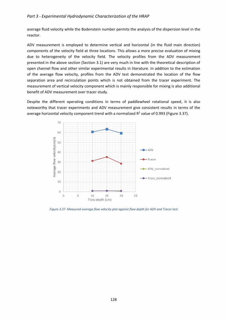
Part 3 - Experimental Hydrodynamic Characterization of the HRAP

128

average fluid velocity while the Bodenstein number permits the analysis of the dispersion level in the

reactor.

ADV measurement is employed to determine vertical and horizontal (in the fluid main direction)

components of the velocity field at three locations. This allows a more precise evaluation of mixing

due to heterogeneity of the velocity field. The velocity profiles from the ADV measurement

presented in the above section (Section 3.1) are very much in line with the theoretical description of

open channel flow and other similar experimental results in literature. In addition to the estimation

of the average flow velocity, profiles from the ADV test demonstrated the location of the flow

separation area and recirculation points which is not obtained from the tracer experiment. The

measurement of vertical velocity component which is mainly responsible for mixing is also additional

benefit of ADV measurement over tracer study.

Despite the different operating conditions in terms of paddlewheel rotational speed, it is also

noteworthy that tracer experiments and ADV measurement give consistent results in terms of the

average horizontal velocity component trend with a normalized R2 value of 0.993 (Figure 3.37).

Figure 3.37- Measured average flow velocity plot against flow depth for ADV and Tracer test

Part 3 - Experimental Hydrodynamic Characterization of the HRAP

129

Part 4 - Inlet Velocity vs Dynamic Mesh Methods for Flow Velocity and Virtual Tracer Simulation in High Rate Algal Pond

130

4 Inlet Velocity vs Dynamic Mesh Methods for Flow Velocity and

Virtual Tracer Simulation in High Rate Algal Pond

4.1 Introduction

Following the remarkable achievements in the area of computing science, Computational Fluid

Dynamics (CFD) modelling has proven itself to offer the possibilities of capturing a wide range of

parameters even in multiphase simulation with a high degree of accuracy including complex pond

hydrodynamics (Bitog et al., 2011; Greifzu et al., 2016; Mendoza et al., 2013a). Since the end of the

20th century, in the area of wastewater technology as well, CFD is becoming a preferable choice

among researchers and application engineers for design and analysis of reactors. Suggesting the

need for complementary work for an improved simulation, (Do-Quang et al., 1998) has applied a

validated CFD model to water and wastewater treatment plants to design a more sustainable

treatment process. Nearly two decades later (Laurent et al., 2014) suggested a protocol for

alternative use of CFD to model physical, chemical and biological processes in wastewater treatment

plants in an integrated manner. An overview by (Samstag et al., 2016) clearly shows how the

technique is then getting attention for analysis and design of almost all unit process in the

wastewater treatment field. A similar review by (Karpinska and Bridgeman, 2016) comprehensively

described some works that have implemented CFD to model aeration of activated sludge tank with a

critical analysis on how CFD data could be coupled with biokinetics in the actual flow field and the

effect on oxygen mass transfer rate. (Rehman et al., 2014) has also integrated CFD with a biokinetic

model on a full-scale wastewater treatment plant to identify regions of bad mixing, their potential

impact and to suggest a simplified improved model of the treatment plant.

Tracer tests are usually considered as a very good way to validate CFD models (Belalcazar et al., 2011;

McClure et al., 2015). This is usually achieved by comparing residence time distribution (RTD) curves

or mixing time derived from experimental tests with numerical tracer simulation. In their detailed

experimental and numerical work, (McClure et al., 2015) demonstrated the tracer injection point and

measurement location had an impact on the mixing time inside a reactor.

In this study, the purpose is to investigate how well the hydrodynamics is represented by two CFD

approaches for representing paddlewheel rotation which induce momentum in the pond.

Simulations are performed using the two methods and then, numerical tracer studies are carried out

and compared to the experimental data showed in the previous chapter. Velocity profiles are also

compared to validate the flow field. Finally, the representation of tracer dispersion as a function of

turbulence (and the turbulent Schmidt number parameter) is discussed.

In the experiment, the tracer is added at the center of the curved channel before the paddlewheel

and measured at the end of the straight channel section next to the paddlewheel in closed flow

conditions. The same injection and measurement (tracer data extraction) sites have been chosen in

the model.

Part 4 - Inlet Velocity vs Dynamic Mesh Methods for Flow Velocity and Virtual Tracer Simulation in High Rate Algal Pond

131

4.2 Comparison of velocity fields

Due to excessive computational time requirements, only the scenario with 20cm depth and

10.76rpm has been implemented in the Dynamic Mesh approach. Hence comparison against Inlet

Velocity is made for this case.

Modelled velocity fields from the Inlet Velocity and Dynamic Mesh methods at the corresponding

mid-depth of the pond for the three cases are presented in Figure 4.1. Both methods were able to

demonstrate high-velocity regions, flow separation points or dead zones, and areas of uniform

velocity distribution at their geometrically anticipated locations.

Except for the increasing velocity magnitude as the depth is reduced from 20 to 10cm, the flow field

shows the same trend in all the three cases of Inlet Velocity method. This result is very similar to the

simulated flow field values of (Hadiyanto et al., 2013) on similar geometry and length to width ratio.

A relatively higher magnitude of the vertical component of the flow velocity that is responsible for

the required vertical mixing was observed at the two curved sections of the pond. The vertical

component of flow velocity was nearly zero in the straight channel sections of the pond except close

to the paddlewheel.

Inlet Velocity

(a)

Dynamic Mesh

(b)

Figure 4.1 - Velocity field (m/s) at the centre of the depth (a) Inlet Velocity, 20cm(top), 15cm (middle) and 10cm (bottom). (b)Dynamic Mesh(20cm)

The velocity applied as an initial condition for the inlet boundary of the Inlet Velocity model

(0.311m/s in the horizontal y-direction only) and the angular speed of the paddlewheel introduced

for the Dynamic Mesh simulation (10.76rpm or 1.13rad/s) was based on the result from the tracer

experiment which was conducted earlier. There was, however, a slight change in the operational

condition of the HRAP during the velocity measurement campaign due to the new power supply

system and motor driving the paddlewheel. This resulted in a clear difference between the model

results and the experimental velocity profiles (Figure 4.2a). In the case of the Dynamic Mesh, the

general profile pattern is still very similar with the measured one. To better illustrate this fact, the

Part 4 - Inlet Velocity vs Dynamic Mesh Methods for Flow Velocity and Virtual Tracer Simulation in High Rate Algal Pond

132

normalized velocity profiles plot of the experimental and the Dynamic Mesh method are presented

below (Figure 4.2c).

Due to the constant velocity imparted on the inlet face of the Inlet Velocity method, the horizontal

velocity profile extracted from the simulation appears to be uniform in almost all the three probed

sites. Though the average velocity predicted by the model (0.308m/s) is close to the average velocity

estimated by tracer experiment (0.29m/s) and is in line with the assumed condition, the simulated

horizontal velocity profile represents nearly an ideal state of uniform velocity distribution.

Dynamic Mesh method, on the other hand, has captured the general trend of the velocity

distribution in the first two locations and considerably deviated from the experimental value in the

third site, as shown in the following figures (Figure 4.2,Figure 4.4 and Figure 4.5). The R2 values for

the three locations are 0.939, 0.909 and 0.524 respectively.

(a) (b)

Figure 4.2 – (a) Inlet Velocity(IV) and Dynamic Mesh(DM) vs Experiment horizontal velocity profile at the first measuring site (b) Dimensionless plot of Dynamic Mesh and Experimental horizontal velocity profile

The inlet boundary condition of the Inlet Velocity simulation is modified similar to the operating

condition of the HRAP during the experimental velocity measurement (Figure 4.3). In this case the

average velocity predicted by the model (0.506m/s) is close the average measured flow velocity

(0.512m/s). As stated before, due to high computational time, such modification to the angular

speed of the paddlewheel couldn’t be made on the Dynamic Mesh method. Based on the

dimensionless curve above (Figure 4.2c), adjusting the model input to the experimental condition

could improve the fitting.

Part 4 - Inlet Velocity vs Dynamic Mesh Methods for Flow Velocity and Virtual Tracer Simulation in High Rate Algal Pond

133

Figure 4.3- Inlet Velocity(IV) and Dynamic Mesh(DM) vs Experiment horizontal velocity profile at the first measuring site for modified inlet boundary

(a) (b)

Figure 4.4– (a) Inlet Velocity(IV) and Dynamic Mesh(DM) vs Experiment horizontal velocity profile at the second measuring site (b) Dimensionless plot of Dynamic Mesh and Experimental horizontal velocity profile

(a) (b)

Figure 4.5– (a) Inlet Velocity(IV) and Dynamic Mesh(DM) vs Experiment horizontal velocity profile at the third measuring site (b) Dimensionless plot of Dynamic Mesh and Experimental horizontal velocity profile

Part 4 - Inlet Velocity vs Dynamic Mesh Methods for Flow Velocity and Virtual Tracer Simulation in High Rate Algal Pond

134

While the velocity prediction by the Dynamic Mesh technique is better than the Inlet Velocity

approach, its computational cost is the biggest obstacle to widely apply it. Enhancing the

performance of Inlet Velocity method by applying the experimental velocity profile on the inlet

boundary instead of assuming a constant value could be a good alternative tool for general design

optimization. OpenFOAM has the functionality to map non-uniform values as an initial condition on

boundaries (see section 4.4).

4.3 Comparison of virtual tracer experiments

Three different depths of flow (10cm, 15cm and 20cm) each with three different paddle-wheel

rotational speeds have been tested in the actual experiment. The same set of depths and

corresponding rotational speeds have been simulated to calculate the flow velocity and to perform

the numerical tracer experiment in the Inlet Velocity method. Contour maps that shows the tracer

material migrating in the reactor presented below (Figure 4.7 - Figure 4.10) are for the 20cm case.

For a steady-state assumption in the Inlet Velocity method, flow fields are calculated from a steady-

state condition that runs until the simulation converges (Table 2.2). The flow field values from the

converged time step are then mapped as an initial condition to solve the scalar transport equation.

Two approaches are tested in the simulation of scalar transport of the tracer material, first by

considering molecular diffusion only and then incorporating the effect of turbulent diffusion.

The model result without considering turbulent diffusivity has underestimated mixing condition in

general. The simulated peak concentrations, as well as the position, were substantially different from

the experimental peak values and pulsation; as shown in (Figure 4.6 Figure 1.1a). Figure 4.7 to Figure

4.10 also show a qualitative difference in tracer diffusion and migration without and with turbulent

diffusion of three different Schmidt number. Sc was reduced from 0.7 to 0.53 and then half the initial

value, 0.35, to increase the diffusivity due to turbulence. Though the peak difference still exists, the

result is much improved for three of the depths of flow tested as shown in Figure 4.6 (b), (c) and (d).

It can be seen from these graphs that considering the turbulent diffusion enables the model to better

predict the mixing time than the model without considering the turbulence effect. The peak value at

Schmidt number 0.35 is slightly closer to the experimental peak than 0.53 and 0.7 (Figure 4.6 d).

In order to interpret these results, it is important to go back to the definition of turbulent Schmidt

number. In RANS, the turbulent transport of momentum is represented by the introduction of the

turbulent (or eddy) viscosity µt. Similarly, turbulent scalar transport is also modeled with a

proportionality with the mean gradient of velocity by introducing turbulent diffusion Γt. As

momentum and scalar transport are both due to turbulence/eddy mixing, the values of µt and Γt are

expected to be of the same order of magnitude. The turbulent Schmidt number is calculated as

𝑆𝑐𝑡 = μ𝑡/Γ𝑡 (Versteeg and Malalasekera, 2007). It describes the ratio of momentum transport

relative to the transport of molecules (Andersson et al., 2011). As the results presented here and as

suggested by several authors (Hreiz et al., 2019; Valero and Bung, 2016), the choice of this parameter

value can be very significant. In field of wastewater treatment application, a value of 0.7 is very often

used by default as suggested by commercial software documentation (e.g. Fluent, 2005). A critical

issue is that this value could be used to compensate for flaws in the velocity field model predictions.

Here, we used a uniform boundary condition for velocity induced by the paddlewheel. Therefore, the

predicted flow field will be more uniform than the experimental one, underestimating the spatial

Part 4 - Inlet Velocity vs Dynamic Mesh Methods for Flow Velocity and Virtual Tracer Simulation in High Rate Algal Pond

135

dispersion. Reducing Sct value partially compensate for this simplification hypothesis, yielding an

improvement of the tracer test prediction to some extent.

(a) (b)

(c) (d) Figure 4.6- Normalized tracer concentration plot over time for 20cm depth (a) without turbulence diffusion (b) Sc=0.7, (c)

Sc=0.53, and (d) Sc=0.35 (Inlet Velocity)

The relatively higher turbulent zones of the pond are the two curved sections and where the

paddlewheel is mounted. As described before, the paddle-wheel region which is slightly lower than

its diameter (73cm), depending on the depth of flow, is replaced by a straight channel of constant

velocity in the Inlet Velocity method. This is supposed to be one of the main reasons behind the

lower diffusion rate in the model output. Though not ascertained by this study the injection manner

could also be another reason. During the experimental work, the salt solution is added into the

flowing water approximately at the center of the depth within a few seconds. However, in the

numerical model, a virtual tracer is placed exactly at the center of the depth all at the same time.

For a fair comparison with the 20cm depth case of the Inlet Velocity approach, all conditions were

kept the same, including the injection location and injection manner while performing the numerical

tracer test in the Dynamic Mesh method. Unlike the previous case, the scalar transport equation is

Part 4 - Inlet Velocity vs Dynamic Mesh Methods for Flow Velocity and Virtual Tracer Simulation in High Rate Algal Pond

136

coupled and simultaneously solved by the transient multiphase solver. This and the additional nodes

for the gas phase make the calculation computationally very intensive.

Flow simulation and scalar transport of the tracer start together from a static condition and gradually

reached to a fully developed transient flow in the case of the Dynamic Mesh method. This makes the

virtual tracer result to show some delay with the experimental one for the first few pick values

(Figure 11). Also, probably due to the instability of the simulation during the first 100 seconds, the

pulse rate is not well-fitting with the experimental tracer curve. This is not the case in the Inlet

Velocity approach that makes it more like the experiment and impressive over Dynamic Mesh, in

addition to the low computational requirements. In general, however, the tracer has been diffused

faster in the Dynamic Mesh method. Hence, compared to the Inlet Velocity method, the mixing time

is quicker by nearly 45%.

Part 4 - Inlet Velocity vs Dynamic Mesh Methods for Flow Velocity and Virtual Tracer Simulation in High Rate Algal Pond

137

(a)

(b)

(c)

(d)

Figure 4.7- (a) Tracer contour map in the reactor without considering turbulent diffusion (20cm flow depth, at mid depth) at different time (0, 5, 40, and 200 seconds top to bottom) Figure 4.8- (b) Tracer contour map in the reactor considering turbulent diffusion Sc=0.7 (20cm flow depth, at mid depth) at different time (0, 5, 40, and 200 seconds top to bottom) Figure 4.9- (c) Tracer contour map in the reactor considering turbulent diffusion Sc=0.53 (20cm flow depth, at mid depth) at different time (0, 5, 40, and 200 seconds top to bottom)

Figure 4.10- (d) Tracer contour in the reactor considering turbulent diffusion Sc=0.35 (20cm flow depth, at mid depth) at different time (0, 5, 40, and 200 seconds top to bottom)

Part 4 - Inlet Velocity vs Dynamic Mesh Methods for Flow Velocity and Virtual Tracer Simulation in High Rate Algal Pond

138

Figure 4.11- Normalized tracer concentration plot over time for 20cm depth (Dynamic Mesh)

As described in section 2.5.5, for the virtual tracer simulation, a different version of OpenFOAM with

additional feature of constraining the tracer material in the liquid zone, is used. This version

(OpenFOAM-v1812 from ESI) couples the scalar transport equation with the main transient

multiphase solver. In the model result, the diffusion of the tracer element is improved that gives very

similar mixing time with the experiment. However, for a reason not clearly understood yet, the result

shows the numerical tracer material is being transported slower than the actual velocity field.

Figure 4.11 demonstrates how the tracer material is traveling slowly in the model. This situation can

also be observed by comparing the contour map of the Dynamic Mesh method with the Inlet velocity

approach, such as Figure 4.12b and Figure 4.8b that shows the tracer distribution 5 seconds after the

injection. The circulation time estimated from the experimental study is around 11.3seconds.

Contrary to this, the dynamic mesh model predicted the circulation time to 31seconds. In fact, the

initial condition in the model and the experiment just before the injection of the tracer element is

different. In the case of the experiment, injection is made while the flow is going on normally

(pseudo steady state). However, in the dynamic mesh simulation, tracer was kept at the injection site

when the simulation starts from a stationary state, before a fully developed flow condition is

achieved. This caused the first peak to be delayed but not expected to retard the general tracer

migration. The problem could be in the version of OpenFOAM while coupling the main solver with

the transport equation.

Part 4 - Inlet Velocity vs Dynamic Mesh Methods for Flow Velocity and Virtual Tracer Simulation in High Rate Algal Pond

139

(a)

(b)

(c)

(d)

(e)

(f)

Figure 4.12- Tracer contour map in the reactor (20cm flow depth, at mid depth) at different times (a) 0s, (b) 5s, (c) 10s, (d) 20s, (e) 40s, and (f) 200s for Dynamic Mesh

Part 4 - Inlet Velocity vs Dynamic Mesh Methods for Flow Velocity and Virtual Tracer Simulation in High Rate Algal Pond

140

4.4 Improving the Inlet Velocity Method

4.4.1 Motivation

Previous results show that the dynamic mesh method gives more accurate results than the inlet

velocity method in terms of predicting the velocity field. It could better represent the 3D velocity

field heterogeneities as well as the turbulence effects on the tracer dispersion. However, this comes

with a very high computational cost. For the final size of the mesh (1.1M grid cell), 32 processors on

the University of Strasbourg HPC were used to simulate the Dynamic Mesh case and the coupled

scalar transport equation. The total time consumed to complete 200s simulation was one month and

2 weeks. Also, the scalar transport that was coupled to the dynamic mesh method did not consider

the turbulent diffusion, giving at the end inaccurate results.

Depending on the objective of the simulation exercise, one can consider choosing between the two

approaches:

1. In case of optimization of the paddlewheel geometry, the dynamic mesh method is

unavoidable;

2. In case of optimization of the design of HRAP shape (middle wall, deflectors…) or if coupling

with scalar transport + reactions is foreseen, the inlet velocity method is preferable;

One intermediate approach is to improve the inlet velocity method by setting up a non-uniform

velocity distribution at the virtual inlet/outlet boundaries. This information could come either from

experimental measures if available or results from a previous simulation. For example, running only

one simulation with the dynamic mesh method could give a realistic velocity field to map as an input

for several other simulations with inlet velocity method.

In OpenFOAM, this type of boundary condition is processed like in the following example:

Starting from initial data of velocity in the y and z directions respectively (Figure 4.13), create a CSV

file with 4 columns: 1 for the depth, 3 for the 3 components of velocity.

(a)

(b)

Figure 4.13 - Sample velocity profiles for improved inlet velocity method (a) y direction (b) z direction

Part 4 - Inlet Velocity vs Dynamic Mesh Methods for Flow Velocity and Virtual Tracer Simulation in High Rate Algal Pond

141

The CSV file looks like:

reference (m);x;y;z 0;0;0.30098712;0.04454065 0.002153632;0;0.31040931;0.03408823 0.004307264;0;0.32022327;0.03825627 0.006460896;0;0.32724605;0.00897256 0.008614528;0;0.33251625;0.02851082 0.01076816;0;0.33720571;0.0311394 0.012921792;0;0.34074069;0.03449823 0.015075424;0;0.34619046;-0.02982804 0.017229056;0;0.34988743;0.02067933 0.019382688;0;0.3534403;0.10950096 0.02153632;0;0.35592589;0.11891253 0.023689951;0;0.35804703;0.12303504 0.025843583;0;0.36198324;0.12816507 0.027997215;0;0.36407422;0.13019661 […] 0.2;0;0.43149356;0.40922382

This file has to be copied in the 0/ folder of the OpenFOAM case. Then the boundary is specified in

the boundaryField section of the U/ file like following:

Figure 4.14 - Example of velocity profile boundary condition specification

Part 4 - Inlet Velocity vs Dynamic Mesh Methods for Flow Velocity and Virtual Tracer Simulation in High Rate Algal Pond

142

In the post processing utility of OpenFOAM (Paraview), this looks like:

Figure 4.15 - Improved inlet velocity method by specifying a non-uniform boundary condition

4.4.2 Obtained results

Figure 4.16 and Figure 4.17 display the velocity profiles obtained by the three methods at the two

first measuring sites:

• Uniform inlet velocity (IV)

• Non-uniform inlet velocity bases on experimental profile (IV_exp)

• Dynamic mesh (DM)

As expected, the updated inlet velocity method gave better prediction of the flow field.

Figure 4.16- Inlet Velocity method prediction using experimental velocity profile at the inlet patch (First measuring point)

Part 4 - Inlet Velocity vs Dynamic Mesh Methods for Flow Velocity and Virtual Tracer Simulation in High Rate Algal Pond

143

Figure 4.17- Inlet Velocity method prediction using experimental velocity profile at the inlet patch (Second measuring point)

Figure 4.18 displays the results of virtual tracer experiments carried out using the converged velocity

and turbulent viscosity fields with non-uniform boundary inlet condition. The most important

conclusion is that the simulation not considering turbulent diffusion is giving totally inaccurate

results in this context: indeed, tracer concentration is monitored during this simulation at one single

location (corresponding to the conductivity probe location in the actual experiment). As highlighted

in Figure 4.7, the tracer will not mix realistically and will remain as a “spot” which is advected

through the reactor: its concentration will not be homogenous in the vertical or horizontal directions,

yielding these erratic results. Once turbulent diffusion is accounted for, the curve is smoother.

However, the different value of Sct affect the global curve shape to a little extent. This suggest that,

in the HRAP, the value of the turbulent Schmidt number is not a so sensitive parameter towards

mixing time simulations if one considers a realistic velocity field provided by the paddlewheel. The

most sensitive parameter affecting the overall dispersion in the system is probably the spatial

dispersion due to flow field heterogeneity.

Figure 4.18 - Impact of turbulent Schmidt number on virtual tracer experiment (Uaverage = 0.311 m/s, 20 cm depth)

Part 4 - Inlet Velocity vs Dynamic Mesh Methods for Flow Velocity and Virtual Tracer Simulation in High Rate Algal Pond

144

In order to investigate this assumption, virtual tracer experiments were carried out assuming a

uniform velocity distribution at the virtual inlet boundary. The corresponding tracer curve is

compared to the previous one with a Sct value of 0.7 (Figure 4.19):

Figure 4.19 - Impact of uniformity of inlet boundary on virtual tracer experiment (Uaverage = 0.311 m/s, 20 cm depth) and comparison with experimental data

From this figure, the uniformity of the inlet boundary condition yields a lower level of dispersion.

Estimation of Bodenstein number through Voncken model confirm this hypothesis. Bo for the non-

uniform boundary is estimated at 115. For the uniform boundary, its value is 165. Also, the mixing

time using the uniform boundary is overestimated (around 130s against 60s for experimental and

non-uniform boundary condition).

From these results, spatial dispersion displays a higher sensitivity when performing a virtual tracer

test in a pond geometry.

However, as shown in Figure 4.19, even the improved boundary condition did not result in an

accurate prediction of the experimental tracer curve. This first sharp peak in the simulation was not

detected in the experiment. As already mentioned in the experimental section, prediction of the first

peaks of a mixing time tracer experiment can be tricky as it will be affected by tracer injection

manner, here in both numerical and physical experiment.

4.5 Conclusions

In this study, two alternative modeling approaches have been assessed to represent the paddlewheel

mixing in a pilot-scale HRAP. Velocity measurements and tracer studies have been carried out to

validate both modeling options.

Part 4 - Inlet Velocity vs Dynamic Mesh Methods for Flow Velocity and Virtual Tracer Simulation in High Rate Algal Pond

145

The simulated velocity field in the Inlet Velocity method shows similar characteristics with expected

flow behaviors at different locations in the pond and with other similar researches. Dead zones are

also clearly shown at the potential flow separation points where the flow makes a sharp turn on

either end of the middle wall. Due to the initial assumptions in this method, however, the horizontal

velocity profiles are not in good agreement with the experimental measurements.

Despite a huge computational time, Dynamic Mesh technique has captured very well the general

flow pattern at the two measuring sites with R2 values of 0.939 and 0.909 but displays a considerable

difference in the third location with R2 of 0.524. This could be due to the short simulation time

making the flow not yet fully developed.

The effect of turbulence in the diffusion of the tracer element has been investigated in the Inlet

Velocity method and it has notably improved the model predictability. In the same method, passive

scalar transport simulation of tracer material is also better fitting with the experimental result when

reducing Turbulent Schmidt Number to 0.35 than 0.53 and 0.7 in terms of peak value as well as

mixing time. The visible difference in peak value could originate from the injection manner and

absence of the paddlewheel mixing effect in the Inlet Velocity approach. The Inlet Velocity method is

considering a uniform velocity profile at the paddlewheel location, this probably underestimate the

spatial dispersion. Lowering Turbulent Schmidt Number value can partly compensate this. However,

if considering turbulent diffusion is mandatory to simulate scalar transport, it is not recommended to

modify Schmidt number value to compensate for oversimplifying assumptions in the simulation.

Due to the difference in the initial condition with the experimental setup and despite the better

velocity field prediction, the Dynamic Mesh method did not capture well the tracer curve. While the

velocity fields are calculated normally, the transport of the tracer material is delayed behind the

experimental tracer movement. A problem of coupling scalar transport function object to the

dynamic mesh transient solver in OpenFOAM might be a cause of this unexpected behavior. Despite

this reality, the mixing time estimation is better in the Dynamic Mesh method. In general, Dynamic

Mesh did not reasonably improve the tracer simulation result when compared with the Inlet Velocity

method in terms of model building complexity and computational time.

Applying the Inlet Velocity method with velocity profile from ADV measurement at the inlet patch

allowed to improve the virtual tracer test accuracy without increasing the computational time to a

high extent. As the flow field is more heterogenous, the spatial dispersion term is increased and

closer to reality. In this condition, turbulent diffusion has still a great influence on the simulation

results, but the sensitivity of turbulent Schmidt number is reduced. Figure 4.18 and Figure 4.19

shows a very interesting improvement of the Inlet Velocity method in predicting the transport of

tracer material. Except at the first pick the tracer plot between the experiment and the model output

is in a very good agreement in terms of peak value, pulsation as well as in estimating the mixing time.

This shows that spatially non-uniform velocity at the boundary has significantly enhanced this

method.

Provided that the inlet boundary condition considers a non-uniform velocity profile, general design

optimization of the pond shape could be assessed using this simplification. Optimizing the design of

the paddlewheel would however be preferably addressed using the Dynamic Mesh method.

Part 5 - Geometrical design modifications

146

5 Geometrical design modifications

In the wastewater treatment field, the usage of CFD has been “traditionally” oriented towards

troubleshooting of existing installations. Nowadays, CFD is used more in the engineering design

phase to refine designs based on rules of thumb and to avoid unexpected behavior after

commissioning.

The following results aims at showing the potential of CFD as a design tool for shape optimization of

a HRAP. Several studies already showed that factors like paddlewheel design, L/W ratio, middle wall

geometry, presence of deflectors, etc. can improve the hydrodynamic efficiency of the HRAP (see

Table 1.7 page 74). However, these studies mainly rely on simplified approaches like Inlet Velocity or

momentum source to describe the momentum induced by the paddlewheel. Here, the non-uniform

boundary condition method described in the previous section will be used (average inlet velocity =

0.311 m/s, depth = 20 cm).

5.1 Pressure and energy consumption

As an example, comparison between the pilot-scale HRAP with and without deflectors at the bends is

presented here.

Figure 5.1 shows the distribution of relative pressure. The pressure at the outlet boundary (in front of

the paddlewheel) is set to zero and the relative pressure here is divided by the density of water (scale

has been changed to improve readability). The abrupt variation of pressure at the bottom of each

image is the location of the inlet velocity boundary. Without deflector, the pressure drop before and

after the paddlewheel is higher. The pressure drops and power consumption of the two designs were

calculated according to Hadiyanto et al. (2013) formula and listed in Table 5.1:

Δ𝑃 = (𝑝𝑖𝑛 − 𝑝𝑜𝑢𝑡)ρ𝑤𝑎𝑡𝑒𝑟

Equation 5-1

The power consumption, W_{cons}, is computed via the formula (Liffman et al 2013):

𝑊𝑐𝑜𝑛𝑠 = Δ𝑃.𝑄 = 0.01206. Δ𝑃

Equation 5-2

With Q the flowrate through the section of the pond

The power consumption of the configuration with deflectors is reduced by 55 %, which is consistent

with the results from Liffman et al. (2013).

(a)

Part 5 - Geometrical design modifications

147

(b)

Figure 5.1 - Relative pressure (in m2/s2) distribution (a) without deflectors (b) with deflectors

Table 5.1 - Pressure loss of one cycle and the required power of paddle wheel

∆𝑃 Wcons

With deflectors 55 Pa 0.66 W

Without deflectors 121 Pa 1.46 W

5.2 Velocity field

Figure 5.2 displays the velocity contours at mid-depth for the two alternative designs. Without

deflectors, a significant part of the HRAP is characterized by low velocities below 0.1 m/s (dark blue

parts). This proportion of “dead-zones” volumes is significantly reduced by the addition of deflectors.

Strong high-speed flow is observed after the bends where flow separation occurs due to the central

wall. With deflectors, this phenomenon is reduced, and the flow is more uniform.

(a)

(b)

Figure 5.2 - Velocity contours at mid-depth (a) without deflectors (b) with deflectors

In addition to energy consumption, the vertical mixing is another important aspect of HRAP design

that can provide recurring access to light to algal cells. Thus, the z component of the velocity field is

plotted at several locations of the HRAP in Figure 5.3. One surprising result is that the configuration

Part 5 - Geometrical design modifications

148

with bends deflectors is providing less vertical mixing than the simpler design. If providing a uniform

velocity field in the horizontal direction is fundamental to avoid dead-zones and minimize energy

consumption, solutions to increase vertical mixing have also to be investigated (optimizing

paddlewheel design, changing the bottom geometry?).

(a)

(b)

Figure 5.3 – z velocity contours (m/s) for different vertical slices (a) without deflectors (b) with deflectors

5.3 Virtual tracer tests

Based on previous simulations, virtual tracer experiments have been performed in a similar way than

in the previous sections (Figure 5.4). With no deflectors, the mixing time is greatly reduced (from 60

to 30s): non-uniformity of the flow field is higher in these conditions in both horizontal and vertical

directions, yielding this faster homogenization. The estimation of Bodenstein number which

decreased from 115 to 34 also confirm the higher level of spatial dispersion in these conditions.

Part 5 - Geometrical design modifications

149

Figure 5.4 - Virtual tracer experiments results for HRAP with and without deflectors at the bends (Sct = 0.7)

5.4 Conclusions

Two HRAP geometrical design have been tested and simulated using CFD: one with the deflectors at

the bends corresponding to the experimental HRAP, the other without these deflectors. The flow

field analysis confirms that the presence of deflectors yields a more uniform horizontal circulation

velocity, leading to less dead-zones volumes inside the pond. In the absence of deflector, there is an

abrupt change in pressure and velocity after the flow pass the curved section of the pond. Since the

flow is not smoothly guided into the straight channel, there is a high chance of flow separation or

extended dead zone behind the middle separating wall leading to a higher speed of flow in the

remaining section of the channel. And the higher the speed of the flow, the higher the energy loss

would be. Hence, without deflector significant energy loss of the flow is observed. Virtual tracer

experiment showed that overall dispersion is lower with the deflectors (less velocity gradient yielding

a lower spatial dispersion).

The pressure drop analysis gave similar results with the literature. The presence of deflectors allowed

to minimize the pressure drop, leading to a 55% reduction in energy consumption. However, the

vertical velocity component is reduced in these conditions, which can decrease recurring light

exposure to algal cells. Future research should focus on multicriteria shape optimization (size,

number and position of deflectors, central wall design, etc.).

Conclusions and Perspectives

151

Conclusions and Perspectives

Conclusions

It has been a while since HRAP is being considered as one promising instrument to neutralize the

future global water and energy challenge due to its simplicity, economy and multitasking character.

Practical reports as well as academical researches surveyed in this work confirmed HRAP has been

applied for various single or multiple purposes in different designs. Even more interesting in those

literatures is the extended interest and effort among researchers and engineers to maximize the

performance of HRAP and to employ it for a relatively new application as an alternative water

resource recovery facility.

In reactors such as HRAP, the treatment of wastewater and recovery of materials is primary

accomplished by the biochemical processes that involves the interaction of organisms in multiphase

media. Furnishing conducive environment only will not lead to an effective reaction. Adequate

interaction between the ingredients which is governed by the hydrodynamics is also a prerequisite in

such multiphase processes. In addition to controlling the mass transfer rate, assisting the exposer of

some elements to solar radiation and avoiding sedimentation, the hydrodynamics is even important

to maintain uniform environmental condition. Quite good number of researches from different

perspectives are made to understand and optimize the effect of the hydrodynamics.

CFD has proven itself to offer the possibilities of capturing wide range of hydrodynamic parameters

even in complex multiphase flows with a high degree of accuracy. Though its widespread application

is relatively young in the field of wastewater engineering, it has been applied to design a new reactor

such as HRAP with efficient shape and to propose optimized power consumption, and also to analyze

an existing plant. The full-scale implementation is still in the initial phase due to high computational

requirements.

One outcome of this research work is that, depending on the modeling objective, a system consisting

of rotating element can be modeled in CFD either in a very simplified way replacing the rotating

element by an equivalent linear speed (Inlet Velocity) or considering a rotating boundary (Dynamic

Mesh). While having high model predictability, the latter is computationally expensive and complex

to set-up. This study compares these two alternative CFD modeling strategies to represent the

paddlewheel of a lab-scale HRAP. Recommended methods are also tested to improve the model

prediction from the simplified approach to propose an easy-to-use and at the same time a reliable

model.

Velocity measurement and tracer study had been carried out to validate both modeling options.

Dynamic Mesh technique has captured very well the general flow pattern at the two measuring sites

with R2 values of 0.939 and 0.909 and has a considerable difference in the third location with R2 of

0.524. This could be due to the short simulation time making the flow not yet fully developed. The

simulated flow velocity contour from both methods shows similar characteristics with expected flow

behaviours at different boundary points of the pond and also with other similar researches in the

literature. Dead zones are clearly indicated at the potential flow separation sites where the flow

makes a sharp turn on either end of the middle separating wall.

Conclusions and Perspectives

152

In the Inlet Velocity method, the average velocities predicted by the model and estimated by the

tracer experiment are very similar. However, due to the constant equivalent velocity assumed at the

inlet boundary, this method did not represent the real velocity profile. Hence, in terms of velocity

prediction, it can be clearly understood that Dynamic Mesh is superior over Inlet Velocity method. To

enhance the velocity prediction from Inlet Velocity method, velocity profile from ADV measurement

has been applied on the inlet patch of the model and better fitting curves are observed in this case.

Virtual tracer simulation results from Dynamic Mesh method showed unexpected behavior probably

due to the discrepancy in coupling the transport equation with the main transient solver. While the

velocity fields are calculated normally, the transport of the tracer material is delayed behind the

experimental tracer movement. However, even though the tracer is hindered, due to the presence of

the actual paddlewheel blending effect, the dispersion condition is very good, and the mixing time is

in good agreement with the experiment.

In the case of Inlet Velocity method, effort is made in this work to modify the existing solver by

including turbulent diffusion term with the molecular diffusion to see how well it can improve

transport modeling in terms of peak value, mixing time and pulsation. Hence, different virtual tracer

tests, introducing different turbulent Schmidt number to calculate the turbulent diffusion coefficient,

have been carried out. Result from these simulations showed that considering turbulent diffusion

enhanced the model prediction of pulse rate, mixing time and reduced the peak value difference

with the experiment. Decreasing values of turbulent Schmidt number allowed to increase model

accuracy by increasing diffusion. However, visible difference in peak values remained, probably due

to the difference in the tracer injection manner and the underestimation of the mixing effect of the

paddlewheel.

Applying the inlet velocity method with velocity profile from ADV measurement at the inlet patch

allowed to improve the virtual tracer test accuracy. As the flow field is more heterogenous, the

spatial dispersion term is increased and closer to reality. In this condition, turbulent diffusion has still

a great influence on the simulation results, but the sensitivity of turbulent Schmidt number is

reduced.

It must be highlighted here that CFD coupling with a biokinetic model also involves coupling with

scalar transport including the different components of dispersion (spatial, turbulent, molecular). This

aspect should therefore be considered accurately in this respect.

In this particular model setup, Dynamic Mesh method didn’t reasonably improve the tracer

simulation result when compared with the Inlet Velocity method in terms of model building

complexity and computational time. If the objective of the modeling exercise is to build a combined

biokinetic/hydrodynamic model, improved Inlet Velocity method with an inlet boundary condition

mapped from experimental result should be sufficient in most cases.

Simple modification has been made on the geometry of the pond to demonstrate the effect of the

flow deflector on mixing condition and power consumption. In line with other studies (Hadiyanto et

al., 2013; Sompech et al., 2012), the provision of deflectors at the curved ends where the flow turns

direction leveled out the velocity distribution thereby reducing the flow separation or formation of

dead zone and the overall power consumption. However, due to the smoother flow field, the vertical

Conclusions and Perspectives

153

component of the velocity is decreased yielding in lower spatial dispersion of tracer. This is

undesirable condition for a real scale HRAP that affects productivity from low light exposure of algal

cells. CFD could therefore help to easily optimize shape and accessories of the pond for possible

minimum power consumption and dead zone formation, and maximum algal productivity.

Perspectives

Solving the flow fields and coupled transport equation of a small pilot HRAP (1.1M cell size) using

Dynamic Mesh technique for 200 seconds consumed more than one-month time on the high-

performance cluster computer (HPC) of the University of Strasbourg with 32 processors. With the

current computational power, the full-scale implementation of Dynamic Mesh method coupled with

other pertinent models such as biokinetic and light irradiance model appears to be impractical for

many engineering applications. Hence, in the near future, improving the Inlet Velocity method

through the understanding and optimizing of the major influencing parameters will make full-scale

coupling of CFD with other models a feasible option.

Algal culture in wastewater by default contains the three phases, the continuous phase (water), and

the dispersed solid and gas phases (suspended solids, biomass, and released gases). To accurately

and effectively simulate these complex interactions between phases and reactions together with the

influencing external factors in CFD, efficient modeling approach in terms of model building,

simulation time and quality result should be proposed to design sustainable HRAP. Compartmental

modeling has emerged as a nice option to intermediate the excessive computational time of CFD and

quality result. Full scale modeling of HRAP could therefore be addressed using this technique in the

future. Future research should also focus on multicriterial shape optimization (size, number and

position of deflectors, central wall design, number and type of paddlewheel blades etc.).

In this study, only one type of turbulence model, K-Ꜫ, has been applied during the numerical

calculation of flow field parameters. K-Ꜫ turbulence model is known for its wide range of applicability

and had been validated in different operating condition. However, despite their heavy computational

load, we recommend other accurate models such as Reynolds stress equation model (RSM) to be

tested in this particular case: this model considers anisotropic turbulence, yielding more realistic

velocity profiles in open-channel conditions.

During the tracer experiment, sodium chloride (NaCl) is used as a tracer material. It is also

recommended to use a dye for visual inspection of the flow structure including flow separation and

recirculation point. It can also give a good idea on how to compartmentalize the total fluid flow

domain before the simulated result.

In addition to the easy access, open source CFD modeling packages provide high degree of flexibility

to simulate a wide range of physical realities. Online forums to assist the learning process and quick

fixing of various challenges in organized manner are another source of motivation to apply them. The

same is true in the case of OpenFOAM. Certain functionalities, however, are not fully standardized

and validated. Choosing the right dictionary type for the mesh motion in Dynamic Mesh method and

constraining the transport of tracer material in one phase of a multiphase flow were among the

biggest challenge during this study. We expect developers are debugging anomalies and resolving the

less standardized functionalities.

Conclusions and Perspectives

154

Certain existing wastewater treatment facilities have already transformed from being energy

efficient to energy recovering or energy positive plants. Their new name, Water Resource Recovery

Facilities, is originated from this added functionality. In general, future advancement in CFD research

and application are yet needed to consolidate the novelty of HRAP as water resource recovery facility

through a continuous optimization of inefficient components and helping the widespread use of such

system in the global scale.

References

155

References

Abbas, H., Nasr, R., Seif, H., 2006. Study of waste stabilization pond geometry for the wastewater treatment efficiency. Ecological Engineering 28, 25–34. https://doi.org/10.1016/j.ecoleng.2006.03.008

Abbott, I.A., Hollenberg, G.J., 1992. Marine Algae of California. Stanford University Press. Abda, F., Azbaid, A., Ensminger, D., Fischer, S., François, P., Schmitt, P., Pallarès, A., 2009. Ultrasonic device for real-time

sewage velocity and suspended particles concentration measurements. Water Sci. Technol. 60, 117–125. https://doi.org/10.2166/wst.2009.281

Ahmad, T., Boyd, C.E., 1988. Design and performance of paddle wheel aerators. Aquacultural Engineering 7, 39–62. https://doi.org/10.1016/0144-8609(88)90037-4

AIAA, A.I. of A.A., 1998. Guide for the Verification and Validation of Computational Fluid Dynamics Simulations. AIAA G-077–1998, AIAA, Reston, VA, USA. [WWW Document]. URL https://infostore.saiglobal.com/en-us/Standards/AIAA-G-077-1998-R2002--93501_SAIG_AIAA_AIAA_195832/ (accessed 12.26.19).

Alexandros, S.I., Akratos, C.S., 2016. Removal of Pathogenic Bacteria in Constructed Wetlands: Mechanisms and Efficiency, in: Ansari, A.A., Gill, S.S., Gill, R., Lanza, G.R., Newman, L. (Eds.), Phytoremediation: Management of Environmental Contaminants, Volume 4. Springer International Publishing, Cham, pp. 327–346. https://doi.org/10.1007/978-3-319-41811-7_17

Al-Hashimi, M.A.I., Hussain, H.T., 2013. Stabilization pond for wastewater treatment. European Scientific Journal 9. Ali, H., Cheema, T.A., Yoon, H.-S., Do, Y., Park, C.W., 2015. Numerical prediction of algae cell mixing feature in raceway

ponds using particle tracing methods. Biotechnol. Bioeng. 112, 297–307. https://doi.org/10.1002/bit.25443 Alvarado, A., Vedantam, S., Goethals, P., Nopens, I., 2012. A compartmental model to describe hydraulics in a full-scale

waste stabilization pond. Water Research 46, 521–530. https://doi.org/10.1016/j.watres.2011.11.038 Amato, T., Wicks, J., 2009. The practical application of computational fluid dynamics to dissolved air flotation, water

treatment plant operation, design and development. Journal of Water Supply: Research and Technology - Aqua 58, 65–73. https://doi.org/10.2166/aqua.2009.003

Amini, H., Hashemisohi, A., Wang, L., Shahbazi, A., Bikdash, M., Kc, D., Yuan, W., 2016. Numerical and experimental investigation of hydrodynamics and light transfer in open raceway ponds at various algal cell concentrations and medium depths. Chemical Engineering Science 156, 11–23. https://doi.org/10.1016/j.ces.2016.09.003

Andersen, R.A., 2005a. Algal Culturing Techniques. Academic Press. Andersen, R.A., 2005b. Algal Culturing Techniques. Academic Press. Anderson, J.D., 1995. Computational Fluid Dynamics, The Basics with Applications, First Edition. ed. McGraw-Hill, Inc.,

USA. Andersson, B., Andersson, R., Hakansson, L., Mortensen, M., Sudiyo, R., van Wachem, B., 2011. Computational Fluid

Dynamics for Engineers. Cambridge University Press, Cambridge. https://doi.org/10.1017/CBO9781139093590 ANSYS FLUENT 12.0, 2009. ANSYS FLUENT 12.0 Theory Guide [WWW Document]. URL

https://www.afs.enea.it/project/neptunius/docs/fluent/html/th/main_pre.htm (accessed 1.15.20). Barbosa, Marco Albrecht, René H. Wijffels, 2003. Hydrodynamic stress and lethal events in sparged microalgae cultures -

Barbosa - 2003 - Biotechnology and Bioengineering - Wiley Online Library [WWW Document]. URL https://onlinelibrary.wiley.com/doi/pdf/10.1002/bit.10657 (accessed 5.27.19).

Barsanti, L., Gualtieri, P., 2014. Algae: anatomy, biochemistry, and biotechnology. CRC press. Bastian, R.K., Hammer, D.A., 2008. The use of constructed wetlands for wastewater treatment and recycling G.A.

Moshiri (Ed.), Constructed wetlands for water quality improvement, Lewis, Boca Raton (1993), pp. 59-68. Beal, C.D., Gardner, E.A., Menzies, N.W., 2005. Process, performance, and pollution potential: A review of septic tank–

soil absorption systems. Soil Res. 43, 781–802. https://doi.org/10.1071/SR05018 Behrens, H., Beims, U., Dieter, H., Dietze, G., Eikmann, T., Grummt, T., Hanisch, H., Henseling, H., Käß, W., Kerndorff, H.,

Leibundgut, C., Müller-Wegener, U., Rönnefahrt, I., Scharenberg, B., Schleyer, R., Schloz, W., Tilkes, F., 2001. Toxicological and ecotoxicological assessment of water tracers. Hydrogeology Journal 9, 321–325. https://doi.org/10.1007/s100400100126

Belalcazar, L.C., Zamudio, A., Clappier, A., Blond, N., Flassak, T., 2011. Validation of a Computational Fluids Dynamics (CFD) model from a roadside long term tracer study, in: The Proceedings of the Air and Waste Management Association’s Annual Conference and Exhibition. pp. 3165–3169.

References

156

Belarbi, E.-H., Molina, E., Chisti, Y., 2000. RETRACTED: A process for high yield and scaleable recovery of high purity eicosapentaenoic acid esters from microalgae and fish oil. Process Biochemistry 35, 951–969. https://doi.org/10.1016/S0032-9592(00)00126-6

Benemann, J.R., 1979. Production of nitrogen fertilizer with nitrogen-fixing blue - green algae. Enzyme and Microbial Technology 1, 83–90. https://doi.org/10.1016/0141-0229(79)90103-0

Bitog, J.P., Lee, I.-B., Lee, C.-G., Kim, K.-S., Hwang, H.-S., Hong, S.-W., Seo, I.-H., Kwon, K.-S., Mostafa, E., 2011. Application of computational fluid dynamics for modeling and designing photobioreactors for microalgae production: A review. Computers and Electronics in Agriculture 76, 131–147. https://doi.org/10.1016/j.compag.2011.01.015

BOKIL, S.D., Bewtra, J.K., 1973. Influence of mechanical blending on aerobic digestion of waste activated sludge, in: Advances in Water Pollution Research. Elsevier, pp. 421–438.

Borowitzka, M.A., 2013. Techno-Economic Modeling for Biofuels from Microalgae, in: Borowitzka, M.A., Moheimani, N.R. (Eds.), Algae for Biofuels and Energy, Developments in Applied Phycology. Springer Netherlands, pp. 255–264. https://doi.org/10.1007/978-94-007-5479-9_15

Borowitzka, M.A., 1999. Commercial production of microalgae: ponds, tanks, tubes and fermenters. Journal of Biotechnology, Biotechnological Aspects of Marine Sponges 70, 313–321. https://doi.org/10.1016/S0168-1656(99)00083-8

Brennan, D., 2001. The Numerical Simulation of Two-Phase Flows in Settling Tanks (PhD). Imperial College, London, UK. Bridgwater, A.V., Toft, A.J., Brammer, J.G., 2002. A techno-economic comparison of power production by biomass fast

pyrolysis with gasification and combustion. Renewable and Sustainable Energy Reviews 6, 181–246. https://doi.org/10.1016/S1364-0321(01)00010-7

Buhr, H.O., Miller, S.B., 1983a. A dynamic model of the high-rate algal-bacterial wastewater treatment pond. Water Research 17, 29–37. https://doi.org/10.1016/0043-1354(83)90283-X

Buhr, H.O., Miller, S.B., 1983b. A dynamic model of the high-rate algal-bacterial wastewater treatment pond. Water Research 17, 29–37. https://doi.org/10.1016/0043-1354(83)90283-X

Butler, D., Digman, C.J., Makropoulos, C., Davies, J.W., Digman, C.J., Makropoulos, C., Davies, J.W., 2018. Urban Drainage. CRC Press. https://doi.org/10.1201/9781351174305

Calheiros, C.S.C., Rangel, A.O.S.S., Castro, P.M.L., 2014. Constructed Wetlands for Tannery Wastewater Treatment in Portugal: Ten Years of Experience. International Journal of Phytoremediation 16, 859–870. https://doi.org/10.1080/15226514.2013.798622

Capodaglio, A.G., Callegari, A., Cecconet, D., Molognoni, D., 2017. Sustainability of decentralized wastewater treatment technologies. Water Practice and Technology 12, 463–477. https://doi.org/10.2166/wpt.2017.055

Cheng, J., Yang, Z., Ye, Q., Zhou, J., Cen, K., 2015. Enhanced flashing light effect with up-down chute baffles to improve microalgal growth in a raceway pond. Bioresource Technology 190, 29–35. https://doi.org/10.1016/j.biortech.2015.04.050

Chisti, Y., 2016. Large-Scale Production of Algal Biomass: Raceway Ponds, in: Bux, F., Chisti, Y. (Eds.), Algae Biotechnology: Products and Processes, Green Energy and Technology. Springer International Publishing, Cham, pp. 21–40. https://doi.org/10.1007/978-3-319-12334-9_2

Chisti, Y., 2007. Biodiesel from microalgae. Biotechnology Advances 25, 294–306. https://doi.org/10.1016/j.biotechadv.2007.02.001

Coggins, L.X., Crosbie, N.D., Ghadouani, A., 2019. The small, the big, and the beautiful: Emerging challenges and opportunities for waste stabilization ponds in Australia. Wiley Interdisciplinary Reviews: Water 6, e1383. https://doi.org/10.1002/wat2.1383

Cole, J.J., 1982. Interactions Between Bacteria and Algae in Aquatic Ecosystems. Annual Review of Ecology and Systematics 13, 291–314. https://doi.org/10.1146/annurev.es.13.110182.001451

Coulter, J.B., 1958. The septic tank system in suburbia. Public Health Rep 73, 488–492. Craggs, R., Park, J., Heubeck, S., Sutherland, D., 2014. High rate algal pond systems for low-energy wastewater

treatment, nutrient recovery and energy production. New Zealand Journal of Botany 52, 60–73. https://doi.org/10.1080/0028825X.2013.861855

Craggs, R.J., Davies-Colley, R.J., Tanner, C.C., Sukias, J.P., 2003. Advanced pond system: performance with high rate ponds of different depths and areas. Water Sci Technol 48, 259–267. https://doi.org/10.2166/wst.2003.0129

Craggs, R.J., Heubeck, S., Lundquist, T.J., Benemann, J.R., 2011. Algal biofuels from wastewater treatment high rate algal ponds. Water Science and Technology 63, 660–665. https://doi.org/10.2166/wst.2011.100

References

157

Crites, R., Technobanoglous, G., 1998. Small and decentralized wastewater management systems. McGraw-Hill. Crites, R.W., Middlebrooks, J., Reed, S.C., 2006. Natural Wastewater Treatment Systems, Taylor & Francis Group, LLC.

Taylor & Francis Group, LLC. Cromar, N.J., Fallowfield, H.J., 1997. Effect of nutrient loading and retention time on performance of high rate algal

ponds. Journal of Applied Phycology 9, 301–309. https://doi.org/10.1023/A:1007917610508 Cuellar-Bermudez, S.P., Aleman-Nava, G.S., Chandra, R., Garcia-Perez, J.S., Contreras-Angulo, J.R., Markou, G., Muylaert,

K., Rittmann, B.E., Parra-Saldivar, R., 2017. Nutrients utilization and contaminants removal. A review of two approaches of algae and cyanobacteria in wastewater. Algal Research, Wastewater and Algae; opportunities, challenges and long term sustainability 24, 438–449. https://doi.org/10.1016/j.algal.2016.08.018

Danckwerts, P.V., 1953. Continuous flow systems. Distribution of residence times. Chemical Engineering Science, Frontiers of Chemical Engineering Science 50, 3857–3866. https://doi.org/10.1016/0009-2509(96)81811-2

De Clercq, B., 2003. Computational fluid dynamics of settling tanks: development of experiments and rheological, settling, and scraper submodels. Ghent University, Ghent.

De Clercq, J., Jacobs, F., Kinnear, D.J., Nopens, I., Dierckx, R.A., Defrancq, J., Vanrolleghem, P.A., 2005. Detailed spatio-temporal solids concentration profiling during batch settling of activated sludge using a radiotracer. Water Research 39, 2125–2135. https://doi.org/10.1016/j.watres.2005.03.023

De Schryver, P., Crab, R., Defoirdt, T., Boon, N., Verstraete, W., 2008. The basics of bio-flocs technology: The added value for aquaculture. Aquaculture 277, 125–137. https://doi.org/10.1016/j.aquaculture.2008.02.019

Dellinger, G., Garambois, P.-A., Dellinger, N., Dufresne, M., Terfous, A., Vazquez, J., Ghenaim, A., 2018. Computational fluid dynamics modeling for the design of Archimedes Screw Generator. Renewable Energy 118, 847–857. https://doi.org/10.1016/j.renene.2017.10.093

Denny, P., 1997. Implementation of constructed wetlands in developing countries. Water Sci Technol 35, 27–34. https://doi.org/10.2166/wst.1997.0157

Devolder, B., Schmitt, P., Rauwoens, P., Elsaesser, B., Troch, P., 2015. A review of the implicit motion solver algorithm in OpenFOAM to simulate a heaving Buoy, in: 18th Numerical Towing Tank Symposium, Proceedings. Presented at the NUTTS conference 2015 : 18th Numerical Towing Tank Symposium, pp. 1–6.

Dijkstra, A.J., 2006. Revisiting the formation of trans isomers during partial hydrogenation of triacylglycerol oils. European Journal of Lipid Science and Technology 108, 249–264. https://doi.org/10.1002/ejlt.200500335

Dires, S., Birhanu, T., Ambelu, A., 2019. Use of broken brick to enhance the removal of nutrients in subsurface flow constructed wetlands receiving hospital wastewater. Water Sci Technol 79, 156–164. https://doi.org/10.2166/wst.2019.037

Dodd, J.C., 2017. Elements of pond design and construction, in: Handbook of Microalgal Mass Culture (1986). CRC Press, pp. 265–284.

Donzis, D.A., Aditya, K., Sreenivasan, K.R., Yeung, P.K., 2014. The Turbulent Schmidt Number. J. Fluids Eng 136. https://doi.org/10.1115/1.4026619

Do-Quang, Z., Cockx, A., Liné, A., Roustan, M., 1998. Computational fluid dynamics applied to water and wastewater treatment facility modeling. Environmental Engineering and Policy 1, 137–147. https://doi.org/10.1007/s100220050015

Duduković, M.P., 1986. Tracer Methods in Chemical Reactors. Techniques and Applications, in: de Lasa, H.I. (Ed.), Chemical Reactor Design and Technology: Overview of the New Developments of Energy and Petrochemical Reactor Technologies. Projections for the 90’s, NATO ASI Series. Springer Netherlands, Dordrecht, pp. 107–189. https://doi.org/10.1007/978-94-009-4400-8_5

eawag, 2019. Compendium of Sanitation Systems and Technologies, 2nd Revised Edition [WWW Document]. URL https://www.eawag.ch/en/department/sandec/publications/compendium/ (accessed 11.19.19).

El Ouarghi, H., Boumansour, B.E., Dufayt, O., El Hamouri, B., Vasel, J.L., 2000. Hydrodynamics and oxygen balance in a high-rate algal pond. Water science and technology 42, 349–356.

Eppley, R.W., 1972. Temperature and phytoplankton growth in the sea. Fish. bull 70, 1063–1085. Fang, D., Chen, B., 2017. Linkage analysis for the water–energy nexus of city. Applied Energy 189, 770–779.

https://doi.org/10.1016/j.apenergy.2016.04.020 Fasaei, F., Bitter, J.H., Slegers, P.M., van Boxtel, A.J.B., 2018.- Techno-economic evaluation of microalgae harvesting and

dewatering systems. Algal Research 31, 347–362. https://doi.org/10.1016/j.algal.2017.11.038 Fluent, A., 2005. Gambit User’s Guide, Fluent Inc (2005).

References

158

Fogler, H.S., 2006a. Chapter 13: Distributions of Residence Times for Chemical Reactors, in: Elements of Chemical Reaction Engineering. Prentice Hall PTR.

Fogler, H.S., 2006b. Chapter 14: Models for Nonideal Reactors, in: Elements of Chemical Reaction Engineering. Prentice Hall PTR.

François, P., Locatelli, F., Laurent, J., Bekkour, K., 2016. Experimental study of activated sludge batch settling velocity profile. Flow Measurement and Instrumentation 48, 112–117. https://doi.org/10.1016/j.flowmeasinst.2015.08.009

Frijns, J., Hofman, J., Nederlof, M., 2013. The potential of (waste)water as energy carrier. Energy Conversion and Management, Global Conference on Renewable energy and Energy Efficiency for Desert Regions 2011 “GCREEDER 2011” 65, 357–363. https://doi.org/10.1016/j.enconman.2012.08.023

Gearheart, R.A., 1992. Use of Constructed Wetlands to Treat Domestic Wastewater, City of Arcata, California. Water Sci Technol 26, 1625–1637. https://doi.org/10.2166/wst.1992.0606

Gerardi, M.H., 2003. Nitrification and denitrification in the activated sludge process. John Wiley & Sons. Ghazy, M.M., Senousy, W.M., Aatty, A.M., Kamel, M., 2008. Performance evaluation of a waste stabilization pond in a

rural area in Egypt. American Journal of Environmental Sciences 4, 316. Gijzen, H.J., 2002. Anaerobic digestion for sustainable development: a natural approach. Water Sci Technol 45, 321–328.

https://doi.org/10.2166/wst.2002.0364 Gikas, G.D., Tsihrintzis, V.A., Akratos, C.S., 2011. Performance and modeling of a vertical flow constructed wetland–

maturation pond system. Journal of Environmental Science and Health, Part A 46, 692–708. https://doi.org/10.1080/10934529.2011.571579

Goecke, F., Labes, A., Wiese, J., Imhoff, J.F., 2010. Chemical interactions between marine macroalgae and bacteria. Marine Ecology Progress Series 409, 267–299. https://doi.org/10.3354/meps08607

Gonçalves, A.L., Pires, J.C.M., Simões, M., 2017. A review on the use of microalgal consortia for wastewater treatment. Algal Research, Wastewater and Algae; opportunities, challenges and long term sustainability 24, 403–415. https://doi.org/10.1016/j.algal.2016.11.008

Gonçalves, A.L., Simões, M., Pires, J.C.M., 2014. The effect of light supply on microalgal growth, CO2 uptake and nutrient removal from wastewater. Energy Conversion and Management 85, 530–536. https://doi.org/10.1016/j.enconman.2014.05.085

Gotaas, H.B., Oswald, W.J., Ludwig, H.F., 1954. Photosynthetic Reclamation of Organic Wastes. The Scientific Monthly 79, 368–378.

Grady Jr, C.L., Daigger, G.T., Love, N.G., Filipe, C.D., 2011. Biological wastewater treatment. CRC press. Greenshields, C., 2018. OpenFOAM v6 User Guide: 5.3 Mesh generation - blockMesh [WWW Document]. CFD Direct.

URL https://cfd.direct/openfoam/user-guide/v6-blockmesh/ (accessed 12.31.19). Greifzu, F., Kratzsch, C., Forgber, T., Lindner, F., Schwarze, R., 2016. Assessment of particle-tracking models for dispersed

particle-laden flows implemented in OpenFOAM and ANSYS FLUENT. Engineering Applications of Computational Fluid Mechanics 10, 30–43. https://doi.org/10.1080/19942060.2015.1104266

Griborio, A., 2004. Secondary Clarifier Modeling: A Multi-Process Approach. University of New Orleans Theses and Dissertations.

Grobbelaar, J.U., 2012. Microalgae mass culture: the constraints of scaling-up. J Appl Phycol 24, 315–318. https://doi.org/10.1007/s10811-011-9728-6

Grobbelaar, J.U., 1991. The influence of light/dark cycles in mixed algal cultures on their productivity. Bioresource Technology, Algal biotechnology 38, 189–194. https://doi.org/10.1016/0960-8524(91)90153-B

Grobbelaar, J.U., Soeder, C.J., Stengel, E., 1990. Modeling algal productivity in large outdoor cultures and waste treatment systems. Biomass 21, 297–314. https://doi.org/10.1016/0144-4565(90)90079-Y

Grönlund, E., Klang, A., Falk, S., Hanæus, J., 2004. Sustainability of wastewater treatment with microalgae in cold climate, evaluated with emergy and socio-ecological principles. Ecological Engineering 22, 155–174. https://doi.org/10.1016/j.ecoleng.2004.03.002

Grossart, H.-P., Simon, M., 2007. Interactions of planktonic algae and bacteria: effects on algal growth and organic matter dynamics. Aquatic Microbial Ecology 47, 163–176. https://doi.org/10.3354/ame047163

Guest, J.S., Skerlos, S.J., Barnard, J.L., Beck, M.B., Daigger, G.T., Hilger, H., Jackson, S.J., Karvazy, K., Kelly, L., Macpherson, L., Mihelcic, J.R., Pramanik, A., Raskin, L., Van Loosdrecht, M.C.M., Yeh, D., Love, N.G., 2009. A New Planning and Design Paradigm to Achieve Sustainable Resource Recovery from Wastewater. Environ. Sci. Technol. 43, 6126–6130. https://doi.org/10.1021/es9010515

References

159

Gupta, P.L., Lee, S.-M., Choi, H.-J., 2015. A mini review: photobioreactors for large scale algal cultivation. World J Microbiol Biotechnol 31, 1409–1417. https://doi.org/10.1007/s11274-015-1892-4

Haberl, R., 1999. Constructed wetlands: A chance to solve wastewater problems in developing countries. Water Science and Technology 40, 11–17. https://doi.org/10.1016/S0273-1223(99)00415-1

Haberl, R., Perfler, R., Mayer, H., 1995. Constructed wetlands in Europe. Water Science and Technology, Wetland Systems for Water Pollution Control 1994 32, 305–315. https://doi.org/10.1016/0273-1223(95)00631-1

Hadiyanto, H., Elmore, S., Van Gerven, T., Stankiewicz, A., 2013. Hydrodynamic evaluations in high rate algae pond (HRAP) design. Chemical Engineering Journal 217, 231–239. https://doi.org/10.1016/j.cej.2012.12.015

Harada, H., Dong, N.T., Matsui, S., 2008. A measure for provisional-and-urgent sanitary improvement in developing countries: septic-tank performance improvement. Water Sci Technol 58, 1305–1311. https://doi.org/10.2166/wst.2008.715

Ho, L.T., Van Echelpoel, W., Goethals, P.L.M., 2017. Design of waste stabilization pond systems: A review. Water Research 123, 236–248. https://doi.org/10.1016/j.watres.2017.06.071

Hosetti, B.B., Frost, S., 1995. A review of the sustainable value of effluents and sludges from wastewater stabilization ponds. Ecological Engineering 5, 421–431. https://doi.org/10.1016/0925-8574(95)00005-4

Hreiz, R., Potier, O., Wicks, J., Commenge, J.-M., 2019. CFD Investigation of the effects of bubble aerator layouts on hydrodynamics of an activated sludge channel reactor. Environmental Technology 40, 2657–2670. https://doi.org/10.1080/09593330.2018.1448001

Hreiz, R., Sialve, B., Morchain, J., Escudié, R., Steyer, J.-P., Guiraud, P., 2014a. Experimental and numerical investigation of hydrodynamics in raceway reactors used for algaculture. Chemical Engineering Journal 250, 230–239. https://doi.org/10.1016/j.cej.2014.03.027

Hreiz, R., Sialve, B., Morchain, J., Escudié, R., Steyer, J.-P., Guiraud, P., 2014b. Experimental and numerical investigation of hydrodynamics in raceway reactors used for algaculture. Chemical Engineering Journal 250, 230–239. https://doi.org/10.1016/j.cej.2014.03.027

Hreiz, R., Sialve, B., Morchain, J., Escudié, R., Steyer, J.-P., Guiraud, P., 2014c. Experimental and numerical investigation of hydrodynamics in raceway reactors used for algaculture. Chemical Engineering Journal 250, 230–239. https://doi.org/10.1016/j.cej.2014.03.027

Huang, J., Qu, X., Wan, M., Ying, J., Li, Y., Zhu, F., Wang, J., Shen, G., Chen, J., Li, W., 2015. Investigation on the performance of raceway ponds with internal structures by the means of CFD simulations and experiments. Algal Research 10, 64–71. https://doi.org/10.1016/j.algal.2015.04.012

Huisman, J.M., 2000. Marine plants of Australia. University of Western Australia Press in association with Australian Biological Resources Study, Nedlands, Australia.

Hussain, S.I., Blowes, D.W., Ptacek, C.J., Jamieson-Hanes, J.H., Wootton, B., Balch, G., Higgins, J., 2015. Mechanisms of Phosphorus Removal in a Pilot-Scale Constructed Wetland/BOF Slag Wastewater Treatment System. Environmental Engineering Science 32, 340–352. https://doi.org/10.1089/ees.2014.0376

Irvine, L.M., Chamberlain, Y.M., 1994. Seaweeds of the British Isles: Volume 1 Rhodophyta. Part 2B Corallinales, Hildenbrandiales.

Isenmann, G., 2016. Approche Euler-Lagrange pour la modélisation du transport solide dans les ouvrages de décantation (thesis). Strasbourg.

Jang, E.S., Jung, M.Y., Min, D.B., 2005. Hydrogenation for Low Trans and High Conjugated Fatty Acids. Comprehensive Reviews in Food Science and Food Safety 4, 22–30. https://doi.org/10.1111/j.1541-4337.2005.tb00069.x

Johansen, J.E., Nielsen, P., Sjøholm, C., 1999. Description of Cellulophaga baltica gen. nov., sp. nov. and Cellulophaga fucicola gen. nov., sp. nov. and reclassification of [Cytophaga] lytica to Cellulophaga lytica gen. nov., comb. nov. International Journal of Systematic and Evolutionary Microbiology, 49, 1231–1240. https://doi.org/10.1099/00207713-49-3-1231

Johnson, M., Mara, D.D., 2005. Aerated rock filters for enhanced nitrogen and faecal coliform removal from facultative waste stabilization pond effluents. Water Science and Technology 51, 99–102.

Jorquera, O., Kiperstok, A., Sales, E.A., Embiruçu, M., Ghirardi, M.L., 2010. Comparative energy life-cycle analyses of microalgal biomass production in open ponds and photobioreactors. Bioresource Technology 101, 1406–1413. https://doi.org/10.1016/j.biortech.2009.09.038

Kadlec, R.H., Wallace, S., 2008. Treatment Wetlands. CRC Press. Karpinska, A.M., Bridgeman, J., 2016. CFD-aided modelling of activated sludge systems – A critical review. Water

Research 88, 861–879. https://doi.org/10.1016/j.watres.2015.11.008

References

160

Kennedy, G., Mayer, T., 2002. Natural and constructed wetlands in Canada: An overview. Water Quality Research Journal 37, 295–325.

Ketchum, B.H., Redfield, A.C., 1938. A method for maintaining a continuous supply of marine diatoms by culture. The Biological Bulletin 75, 165–169.

Kisand, V., Tuvikene, L., Nõges, T., 2001. Role of phosphorus and nitrogen for bacteria and phytopankton development in a large shallow lake. Hydrobiologia 457, 187–197. https://doi.org/10.1023/A:1012291820177

Kivaisi, A.K., 2001. The potential for constructed wetlands for wastewater treatment and reuse in developing countries: a review. Ecological Engineering 16, 545–560. https://doi.org/10.1016/S0925-8574(00)00113-0

Knight, R.L., Walton, W.E., O’Meara, G.F., Reisen, W.K., Wass, R., 2003. Strategies for effective mosquito control in constructed treatment wetlands. Ecological Engineering 21, 211–232. https://doi.org/10.1016/j.ecoleng.2003.11.001

Knothe, G., 2006. Analyzing biodiesel: standards and other methods. Journal of the American Oil Chemists’ Society 83, 823–833. https://doi.org/10.1007/s11746-006-5033-y

Kouzuma, A., Watanabe, K., 2015. Exploring the potential of algae/bacteria interactions. Current Opinion in Biotechnology, Environmental biotechnology • Energy biotechnology 33, 125–129. https://doi.org/10.1016/j.copbio.2015.02.007

Krasnovsky, A.A., 2005. Chlorophyll isolation, structure and function: major landmarks of the early history of research in the Russian Empire and the Soviet Union, in: Govindjee, Beatty, J.T., Gest, H., Allen, J.F. (Eds.), Discoveries in Photosynthesis, Advances in Photosynthesis and Respiration. Springer Netherlands, Dordrecht, pp. 1143–1157. https://doi.org/10.1007/1-4020-3324-9_102

Kumar, K., Mishra, S.K., Shrivastav, A., Park, M.S., Yang, J.-W., 2015. Recent trends in the mass cultivation of algae in raceway ponds. Renewable and Sustainable Energy Reviews 51, 875–885. https://doi.org/10.1016/j.rser.2015.06.033

Lakehal, D., Krebs, P., Krijgsman, J., Rodi, W., 1999. Computing Shear Flow and Sludge Blanket in Secondary Clarifiers. J. Hydr. Engrg. 125, 253–262. https://doi.org/10.1061/(ASCE)0733-9429(1999)125:3(253)

Langergraber, G., 2008. Modeling of processes in subsurface flow constructed wetlands: A review. Vadose Zone Journal 7, 830–842.

Larsen, P., 1977. On the Hydraulics of Rectangular Settling Basins: Experimental and Theoretical Studies. Department of Water Resources Engineering, Lund Institute of Technology, University of Lund.

Larsen, T.A., Gujer, W., 1997. The concept of sustainable Urban Water Management. Water Science and Technology, Sustainable Sanitation 35, 3–10. https://doi.org/10.1016/S0273-1223(97)00179-0

Laurent, J., Bois, P., Nuel, M., Wanko, A., 2015. Systemic models of full-scale Surface Flow Treatment Wetlands: Determination by application of fluorescent tracers. Chemical Engineering Journal 264, 389–398. https://doi.org/10.1016/j.cej.2014.11.073

Laurent, J., Samstag, R.W., Ducoste, J.M., Griborio, A., Nopens, I., Batstone, D.J., Wicks, J.D., Saunders, S., Potier, O., 2014. A protocol for the use of computational fluid dynamics as a supportive tool for wastewater treatment plant modelling. Water Sci. Technol. 70, 1575–1584. https://doi.org/10.2166/wst.2014.425

Le Moullec, Y., Potier, O., Gentric, C., Pierre Leclerc, J., 2008. Flow field and residence time distribution simulation of a cross-flow gas–liquid wastewater treatment reactor using CFD. Chemical Engineering Science 63, 2436–2449. https://doi.org/10.1016/j.ces.2008.01.029

Levenspiel, O., 1999a. Chemical Reaction Engineering. Ind. Eng. Chem. Res. 38, 4140–4143. https://doi.org/10.1021/ie990488g

Levenspiel, O., 1999b. Chemical reaction engineering. Wiley. Li, F., Lu, L., Zheng, X., Ngo, H.H., Liang, S., Guo, W., Zhang, X., 2014. Enhanced nitrogen removal in constructed

wetlands: Effects of dissolved oxygen and step-feeding. Bioresource Technology 169, 395–402. https://doi.org/10.1016/j.biortech.2014.07.004

Li, W., Li, L., Qiu, G., 2017. Energy consumption and economic cost of typical wastewater treatment systems in Shenzhen, China. Journal of Cleaner Production, Urban ecological infrastructure for healthier cities: governance, management and engineering 163, S374–S378. https://doi.org/10.1016/j.jclepro.2015.12.109

Li, Y., Horsman, M., Wu, N., Lan, C.Q., Dubois-Calero, N., 2008. Biofuels from Microalgae. Biotechnol Progress 24, 815–820. https://doi.org/10.1021/bp070371k

References

161

Liffman, K., Paterson, D.A., Liovic, P., Bandopadhayay, P., 2013. Comparing the energy efficiency of different high rate algal raceway pond designs using computational fluid dynamics. Chemical Engineering Research and Design 91, 221–226. https://doi.org/10.1016/j.cherd.2012.08.007

Liu, F., 2016. A Thorough Description Of How Wall Functions Are Implemented In OpenFOAM (Proceedings of CFD with OpenSource Software).

Liu, L., Hall, G., Champagne, P., 2016. Effects of Environmental Factors on the Disinfection Performance of a Wastewater Stabilization Pond Operated in a Temperate Climate. Water 8, 5. https://doi.org/10.3390/w8010005

Liu, X., Zhang, J., 2019. Computational Fluid Dynamics: Applications in Water, Wastewater and Stormwater Treatment. Locatelli, F., François, P., Laurent, J., Lawniczak, F., Dufresne, M., Vazquez, J., Bekkour, K., 2015. Detailed Velocity and

Concentration Profiles Measurement During Activated Sludge Batch Settling Using an Ultrasonic Transducer. Separation Science and Technology 50, 1059–1065. https://doi.org/10.1080/01496395.2014.980002

Locatelli, F., Laurent, J., François, P., Dufresne, M., Vazquez, J., Bekkour, K., 2013. Impact de la loi de comportement rhéologique sur la sédimentation en batch de boues activées : approche expérimentale et numérique. La Houille Blanche 31–36. https://doi.org/10.1051/lhb/2013030

Luo, S., Berges, J.A., He, Z., Young, E.B., 2017. Algal-microbial community collaboration for energy recovery and nutrient remediation from wastewater in integrated photobioelectrochemical systems. Algal Research, Wastewater and Algae; opportunities, challenges and long term sustainability 24, 527–539. https://doi.org/10.1016/j.algal.2016.10.006

Luo, Y., Le-Clech, P., Henderson, R.K., 2017. Simultaneous microalgae cultivation and wastewater treatment in submerged membrane photobioreactors: A review. Algal Research, Wastewater and Algae; opportunities, challenges and long term sustainability 24, 425–437. https://doi.org/10.1016/j.algal.2016.10.026

Maktabifard, M., Zaborowska, E., Makinia, J., 2018. Achieving energy neutrality in wastewater treatment plants through energy savings and enhancing renewable energy production. Rev Environ Sci Biotechnol 17, 655–689. https://doi.org/10.1007/s11157-018-9478-x

Mantovani, M., Marazzi, F., Fornaroli, R., Bellucci, M., Ficara, E., Mezzanotte, V., 2019. Outdoor pilot-scale raceway as a microalgae-bacteria sidestream treatment in a WWTP. Science of The Total Environment 135583. https://doi.org/10.1016/j.scitotenv.2019.135583

Mantovi, P., Marmiroli, M., Maestri, E., Tagliavini, S., Piccinini, S., Marmiroli, N., 2003. Application of a horizontal subsurface flow constructed wetland on treatment of dairy parlor wastewater. Bioresource Technology 88, 85–94. https://doi.org/10.1016/S0960-8524(02)00291-2

Mara, D., 2003. Domestic Wastewater Treatment in Developing Countries, published by Earthscan. Mara, D.D., Cogman, C.A., Simkins, P., Schembri, M.C.A., 1998. Performance of the Burwarton Estate waste stabilization

ponds. Water and Environment Journal 12, 260–264. Martín, J., Santos, J.L., Aparicio, I., Alonso, E., 2015. Pharmaceutically active compounds in sludge stabilization

treatments: Anaerobic and aerobic digestion, wastewater stabilization ponds and composting. Science of The Total Environment, Towards a better understanding of the links between stressors, hazard assessment and ecosystem services under water scarcity 503–504, 97–104. https://doi.org/10.1016/j.scitotenv.2014.05.089

Mata, T.M., Martins, A.A., Caetano, N.S., 2010. Microalgae for biodiesel production and other applications: A review. Renewable and Sustainable Energy Reviews 14, 217–232. https://doi.org/10.1016/j.rser.2009.07.020

Matamoros, V., Gutiérrez, R., Ferrer, I., García, J., Bayona, J.M., 2015. Capability of microalgae-based wastewater treatment systems to remove emerging organic contaminants: A pilot-scale study. Journal of Hazardous Materials 288, 34–42. https://doi.org/10.1016/j.jhazmat.2015.02.002

Mburu, N., Tebitendwa, S.M., van Bruggen, J.J.A., Rousseau, D.P.L., Lens, P.N.L., 2013. Performance comparison and economics analysis of waste stabilization ponds and horizontal subsurface flow constructed wetlands treating domestic wastewater: A case study of the Juja sewage treatment works. Journal of Environmental Management 128, 220–225. https://doi.org/10.1016/j.jenvman.2013.05.031

Mbwele, L., Rubindamayugi, M., Kivaisi, A., Dalhammar, G., 2004. Performance of a small wastewater stabilisation pond system in tropical climate in Dar es Salaam, Tanzania. Water Sci Technol 48, 187–191. https://doi.org/10.2166/wst.2004.0836

McClure, D.D., Aboudha, N., Kavanagh, J.M., Fletcher, D.F., Barton, G.W., 2015. Mixing in bubble column reactors: experimental study and CFD modeling. Chemical Engineering Journal 264, 291–301.

McGinnis, R.L., Elimelech, M., 2008. Global Challenges in Energy and Water Supply: The Promise of Engineered Osmosis. Environ. Sci. Technol. 42, 8625–8629. https://doi.org/10.1021/es800812m

References

162

Mendoza, J.L., Granados, M.R., de Godos, I., Acién, F.G., Molina, E., Banks, C., Heaven, S., 2013a. Fluid-dynamic characterization of real-scale raceway reactors for microalgae production. Biomass and Bioenergy 54, 267–275. https://doi.org/Mendoza, J.L., Granados, M.R., de Godos, I., Acién, F.G., Molina, E., Banks, C. and Heaven, S. (2013) Fluid-dynamic characterization of real-scale raceway reactors for microalgae production Biomass and Bioenergy, 54, pp. 267-275. (doi:10.1016/j.biombioe.2013.03.017 <http://dx.doi.org/10.1016/j.biombioe.2013.03.017>).

Mendoza, J.L., Granados, M.R., de Godos, I., Acién, F.G., Molina, E., Banks, C., Heaven, S., 2013b. Fluid-dynamic characterization of real-scale raceway reactors for microalgae production. Biomass and Bioenergy 54, 267–275. https://doi.org/10.1016/j.biombioe.2013.03.017

Mendoza, J.L., Granados, M.R., de Godos, I., Acién, F.G., Molina, E., Heaven, S., Banks, C.J., 2013c. Oxygen transfer and evolution in microalgal culture in open raceways. Bioresource Technology 137, 188–195. https://doi.org/10.1016/j.biortech.2013.03.127

Menter, F.R., 2012. Two-equation eddy-viscosity turbulence models for engineering applications. AIAA Journal. https://doi.org/10.2514/3.12149

Miller, H.O., Buhr, S.B.&, 1981. Mixing characteristics of a high-rate algae pond. Water SA 7, 08-15. Mohd Udaiyappan, A.F., Abu Hasan, H., Takriff, M.S., Sheikh Abdullah, S.R., 2017. A review of the potentials, challenges

and current status of microalgae biomass applications in industrial wastewater treatment. Journal of Water Process Engineering 20, 8–21. https://doi.org/10.1016/j.jwpe.2017.09.006

Monte, M.H.D.M., 1992. Waste Stabilization Ponds in Europe - Water and Environment Journal - Wiley Online Library [WWW Document]. URL https://onlinelibrary.wiley.com/doi/abs/10.1111/j.1747-6593.1992.tb00708.x (accessed 11.12.19).

Montemezzani, V., Duggan, I.C., Hogg, I.D., Craggs, R.J., 2017. Screening of potential zooplankton control technologies for wastewater treatment High Rate Algal Ponds. Algal Research 22, 1–13. https://doi.org/10.1016/j.algal.2016.11.022

Morris, M., Herbert, R., 1997. The design and performance of avertical flow reed bed for the treatment of high ammonia, low suspended solids organic effluents. Water Science and Technology, Wetland Systems for Water Pollution Control 1996 35, 197–204. https://doi.org/10.1016/S0273-1223(97)00069-3

Muñoz, R., Guieysse, B., 2006. Algal–bacterial processes for the treatment of hazardous contaminants: A review. Water Research 40, 2799–2815. https://doi.org/10.1016/j.watres.2006.06.011

MWEA, 2017. Michigan Water Environment Association [WWW Document]. URL https://www.mi-wea.org/# (accessed 11.3.19).

Nopens, I., Batstone, D.J., Griborio, A., Samstag, R., Wicklein, E., Wicks, J., 2012. Computational Fluid Dynamics (CFD): What is Good CFD-Modeling Practice and What Can Be the Added Value of CFD Models to WWTP Modeling? Proceedings of the Water Environment Federation 2012, 7400–7405. https://doi.org/10.2175/193864712811704161

OpenCFD, 2011. OpenFOAM® - Official home of The Open Source Computational Fluid Dynamics (CFD) Toolbox [WWW Document]. URL http://www.openfoam.com (accessed 1.3.20).

Oswald, W.J., 1991. Introduction to Advanced Integrated Wastewater Ponding Systems. Water Sci Technol 24, 1–7. https://doi.org/10.2166/wst.1991.0106

OSWALD, W.J., 1988. Large-scale algal culture systems (engineering aspects). Micro-algal biotechnology. 357–394. Oswald, W.J., Gotaas, H.B., Golueke, C.G., Kellen, W.R., Gloyna, E.F., Hermann, E.R., 1957. Algae in Waste Treatment

[with Discussion]. Sewage and Industrial Wastes 29, 437–457. Ouali, A., Jupsin, H., Vasel, J.L., Ghrabi, A., 2015. Removal of E. coli and enterococci in maturation pond and kinetic

modelling under sunlight conditions. Desalination and Water Treatment 53, 1068–1074. https://doi.org/10.1080/19443994.2013.856350

Ouazzani, N., Bouhoum, K., Mandi, L., Bouarab, L., Habbari, K., Rafiq, F., Picot, B., Bontoux, J., Schwartzbrod, J., 1995. Wastewater treatment by stabilization pond: marrakesh experiment. Water Science and Technology, Waste Stabilisation Ponds and the Reuse of Pond Effluents 31, 75–80. https://doi.org/10.1016/0273-1223(95)00494-8

Pandey, R., Premalatha, M., 2017. Design and analysis of flow velocity distribution inside a raceway pond using computational fluid dynamics. Bioprocess Biosyst Eng 40, 439–450. https://doi.org/10.1007/s00449-016-1712-8

Panepinto, D., Fiore, S., Zappone, M., Genon, G., Meucci, L., 2016. Evaluation of the energy efficiency of a large wastewater treatment plant in Italy. Applied Energy 161, 404–411. https://doi.org/10.1016/j.apenergy.2015.10.027

References

163

Park, J.B.K., Craggs, R.J., 2010. Wastewater treatment and algal production in high rate algal ponds with carbon dioxide addition. Water Sci Technol 633–639. https://doi.org/10.2166/wst.2010.951

Park, J.B.K., Craggs, R.J., Shilton, A.N., 2011. Wastewater treatment high rate algal ponds for biofuel production. Bioresource Technology, Special Issue: Biofuels - II: Algal Biofuels and Microbial Fuel Cells 102, 35–42. https://doi.org/10.1016/j.biortech.2010.06.158

Park, J.B.K., Craggs, R.J., Shilton, A.N., 2010. Wastewater treatment high rate algal ponds for biofuel production. Bioresource Technology, Special Issue: Biofuels - II: Algal Biofuels and Microbial Fuel Cells 102, 35–42. https://doi.org/10.1016/j.biortech.2010.06.158

Park, J.B.K., Craggs, R.J., Tanner, C.C., 2018. Eco-friendly and low-cost Enhanced Pond and Wetland (EPW) system for the treatment of secondary wastewater effluent. Ecological Engineering 120, 170–179. https://doi.org/10.1016/j.ecoleng.2018.05.029

Park, S., Li, Y., 2015. Integration of biological kinetics and computational fluid dynamics to model the growth of Nannochloropsis salina in an open channel raceway. Biotechnology and bioengineering 112, 923–933.

Park, S.Y., 2014. Modeling and Experimental Study of an Open Channel Raceway System to Improve the Performance of Nannochloropsis salina Cultivation (PhD Thesis). Ohio State University.

Pearson, H.W., Mara**, D.D., Arridge*, H.A., 1995. The influence of pond geometry and configuration on facultative and maturation waste stabilisation pond performance and efficiency. Water Science and Technology, Waste Stabilisation Ponds and the Reuse of Pond Effluents 31, 129–139. https://doi.org/10.1016/0273-1223(95)00500-M

Peña, M.R., Mara, D.D., Sanchez, A., 2000. Dispersion studies in anaerobic ponds: implications for design and operation. Water Sci Technol 42, 273–282. https://doi.org/10.2166/wst.2000.0660

Pham, L.A., Laurent, J., Bois, P., Wanko, A., 2018. Impacts of operational conditions on oxygen transfer rate, mixing characteristics and residence time distribution in a pilot scale high rate algal pond. Water Sci Technol 78, 1782–1791. https://doi.org/10.2166/wst.2018.461

Picot, B., Andrianarison, T., Gosselin, J.P., Brissaud, F., 2005. Twenty years’ monitoring of Mèze stabilisation ponds: part I – removal of organic matter and nutrients. Water Sci Technol 51, 23–31. https://doi.org/10.2166/wst.2005.0419

Pittman, J.K., Dean, A.P., Osundeko, O., 2011. The potential of sustainable algal biofuel production using wastewater resources. Bioresource Technology, Special Issue: Biofuels - II: Algal Biofuels and Microbial Fuel Cells 102, 17–25. https://doi.org/10.1016/j.biortech.2010.06.035

Porterfield, W.M., 1922. References to the Algae in the Chinese Classics. Bulletin of the Torrey Botanical Club 49, 297–300. https://doi.org/10.2307/2480100

Prussi, M., Buffi, M., Casini, D., Chiaramonti, D., Martelli, F., Carnevale, M., Tredici, M.R., Rodolfi, L., 2014. Experimental and numerical investigations of mixing in raceway ponds for algae cultivation. Biomass and Bioenergy 67, 390–400. https://doi.org/10.1016/j.biombioe.2014.05.024

Pruvost, J., Pottier, L., Legrand, J., 2006. Numerical investigation of hydrodynamic and mixing conditions in a torus photobioreactor. Chemical Engineering Science 61, 4476–4489. https://doi.org/10.1016/j.ces.2006.02.027

Qasaimeh, A., AlSharie, H., Masoud, T., 2015. A Review on Constructed Wetlands Components and Heavy Metal Removal from Wastewater. Journal of Environmental Protection 6, 710–718. https://doi.org/10.4236/jep.2015.67064

Quijano, G., Arcila, J.S., Buitrón, G., 2017. Microalgal-bacterial aggregates: Applications and perspectives for wastewater treatment. Biotechnology Advances 35, 772–781. https://doi.org/10.1016/j.biotechadv.2017.07.003

Ragonese, F.P., Williams, J.A., 1968. A mathematical model for the batch reactor kinetics of algae growth. Biotechnology and Bioengineering 10, 83–88.

Rasdi, N.W., Qin, J.G., 2015. Effect of N:P ratio on growth and chemical composition of Nannochloropsis oculata and Tisochrysis lutea. J Appl Phycol 27, 2221–2230. https://doi.org/10.1007/s10811-014-0495-z

Reay, D.S., Nedwell, D.B., Priddle, J., Ellis-Evans, J.C., 1999. Temperature Dependence of Inorganic Nitrogen Uptake: Reduced Affinity for Nitrate at Suboptimal Temperatures in Both Algae and Bacteria. Appl. Environ. Microbiol. 65, 2577–2584.

Rehman, U., Amerlinck, Y., Arnaldos, M., Nopens, I., 2014. CFD and Biokinetic Model Integration Applied to a Full Scale WWTP. Proceedings of the Water Environment Federation 2014, 6894–6905. https://doi.org/10.2175/193864714815941649

References

164

Richardson, J.W., Johnson, M.D., Outlaw, J.L., 2012. Economic comparison of open pond raceways to photo bio-reactors for profitable production of algae for transportation fuels in the Southwest. Algal Research 1, 93–100. https://doi.org/10.1016/j.algal.2012.04.001

Richmond, A., 2008. Handbook of microalgal culture: biotechnology and applied phycology. Wiley Online Library. Richmond, A., Grobbelaar, J.U., 1986. Factors affecting the output rate of Spirulina platensis with reference to mass

cultivation. Biomass 10, 253–264. https://doi.org/10.1016/0144-4565(86)90002-8 Rivas, A., Barceló-Quintal, I., Moeller, G.E., 2011. Pollutant removal in a multi-stage municipal wastewater treatment

system comprised of constructed wetlands and a maturation pond, in a temperate climate. Water Sci Technol 64, 980–987. https://doi.org/10.2166/wst.2011.731

Rivas, A., Irizar, I., Ayesa, E., 2008. Model-based optimisation of Wastewater Treatment Plants design. Environmental Modelling & Software 23, 435–450. https://doi.org/10.1016/j.envsoft.2007.06.009

Rosso, D., Larson, L.E., Stenstrom, M.K., 2008. Aeration of large-scale municipal wastewater treatment plants: state of the art. Water Sci Technol 57, 973–978. https://doi.org/10.2166/wst.2008.218

Saidam, M.Y., Ramadan, S.A., Butler, D., 1995. Upgrading waste stabilization pond effluent by rock filters. Water Science and Technology, Waste Stabilisation Ponds and the Reuse of Pond Effluents 31, 369–378. https://doi.org/10.1016/0273-1223(95)00523-P

Samstag, R.W., Ducoste, J.J., Griborio, A., Nopens, I., Batstone, D.J., Wicks, J.D., Saunders, S., Wicklein, E.A., Kenny, G., Laurent, J., 2016. CFD for wastewater treatment: an overview. Water Sci. Technol. 74, 549–563. https://doi.org/10.2166/wst.2016.249

Samstag, R.W., Wicklein, E.A., Reardon, R.D., Leetch, R.J., Parks, R.M., Groff, C.D., 2012. Field and CFD Analysis of Jet Aeration and Mixing. Proceedings of the Water Environment Federation 2012, 4113–4139. https://doi.org/10.2175/193864712811708301

Saqqar, M.M., Pescod, M.B., 1995. Modelling the performance of anaerobic wastewater stabilization ponds - ProQuest [WWW Document]. URL https://search.proquest.com/openview/789b15579fb028bcf56807d103781326/1?pq-origsite=gscholar&cbl=2044520 (accessed 11.13.19).

Schindler, D.W., Hecky, R.E., Findlay, D.L., Stainton, M.P., Parker, B.R., Paterson, M.J., Beaty, K.G., Lyng, M., Kasian, S.E.M., 2008. Eutrophication of lakes cannot be controlled by reducing nitrogen input: results of a 37-year whole-ecosystem experiment. Proceedings of the National Academy of Sciences 105, 11254–11258.

Sells, M.D., Brown, N., Shilton, A.N., 2018. Determining variables that influence the phosphorus content of waste stabilization pond algae. Water Research 132, 301–308. https://doi.org/10.1016/j.watres.2018.01.013

Sharma, M., Thukral, N., Soni, N.K., Maji, S., 2015. Microalgae as Future Fuel: Real Opportunities and Challenges. Journal of Thermodynamics & Catalysis 6, 1–11. https://doi.org/10.4172/2157-7544.1000139

Sharma, P., Sharma, N., 2017. Industrial and Biotechnological Applications of Algae: A Review. JAPB 1, 01. https://doi.org/10.14302/issn.2638-4469.japb-17-1534

Sheehan, J., Dunahay, T., Benemann, J., Roessler, P., 1998. Look Back at the U.S. Department of Energy’s Aquatic Species Program: Biodiesel from Algae; Close-Out Report (No. NREL/TP-580-24190). National Renewable Energy Lab., Golden, CO. (US). https://doi.org/10.2172/15003040

Sheludchenko, M., Padovan, A., Katouli, M., Stratton, H., 2016. Removal of Fecal Indicators, Pathogenic Bacteria, Adenovirus, Cryptosporidium and Giardia (oo)cysts in Waste Stabilization Ponds in Northern and Eastern Australia. International Journal of Environmental Research and Public Health 13, 96. https://doi.org/10.3390/ijerph13010096

Shi, W., Li, H., Li, A., 2018. Mechanism and Influencing Factors of Nitrogen Removal in Subsurface Flow Constructed Wetland. Applied Chemical Engineering 1. https://doi.org/10.24294/ace.v1i1.344

Shih, T.-H., Liou, W.W., Shabbir, A., Yang, Z., Zhu, J., 1995. A new k-ϵ eddy viscosity model for high reynolds number turbulent flows. Computers & Fluids 24, 227–238. https://doi.org/10.1016/0045-7930(94)00032-T

Shin, H.K., Polprasert, C., 1987. Attached-Growth Waste Stabilization Pond Treatment Evaluation. Water Sci Technol 19, 229–235. https://doi.org/10.2166/wst.1987.0150

Shizas Ioannis, Bagley David M., 2004. Experimental Determination of Energy Content of Unknown Organics in Municipal Wastewater Streams. Journal of Energy Engineering 130, 45–53. https://doi.org/10.1061/(ASCE)0733-9402(2004)130:2(45)

Shuib, N., Baskaran, K., Davies, W.R.O., Muthukumaran, S., 2011. Effluent quality performance of horizontal subsurface flow constructed wetlands using natural zeolite (escott).

References

165

Solimeno, A., García, J., 2017. Microalgae-bacteria models evolution: From microalgae steady-state to integrated microalgae-bacteria wastewater treatment models – A comparative review. Science of The Total Environment 607–608, 1136–1150. https://doi.org/10.1016/j.scitotenv.2017.07.114

Sompech, K., Chisti, Y., Srinophakun, T., 2012. Design of raceway ponds for producing microalgae. Biofuels 3, 387–397. https://doi.org/10.4155/bfs.12.39

Spolaore, P., Joannis-Cassan, C., Duran, E., Isambert, A., 2006. Commercial applications of microalgae. J. Biosci. Bioeng. 101, 87–96. https://doi.org/10.1263/jbb.101.87

Stephens, J.C., 1998. Factors Limiting the Acceptance and Use of Innovative Environmental Technologies: A Case Study of the Solar Aquatics SystemTM(Sas) Technology For Wastewater Treatment. Journal of Environmental Systems 26.

Stillwell, A.S., Hoppock, D.C., Webber, M.E., 2010. Energy Recovery from Wastewater Treatment Plants in the United States: A Case Study of the Energy-Water Nexus. Sustainability 2, 1–18.

Sudarsan, J.S., Annadurai, R., Mukhopadhyay, M., Chakraborty, P., Nithiyanantham, S., 2018. Domestic wastewater treatment using constructed wetland: an efficient and alternative way. Sustain. Water Resour. Manag. 4, 781–787. https://doi.org/10.1007/s40899-017-0164-x

Suh, I.S., Lee, C.-G., 2003. Photobioreactor engineering: Design and performance. Biotechnol. Bioprocess Eng. 8, 313. https://doi.org/10.1007/BF02949274

Sutherland, D.L., Howard-Williams, C., Turnbull, M.H., Broady, P.A., Craggs, R.J., 2015a. Enhancing microalgal photosynthesis and productivity in wastewater treatment high rate algal ponds for biofuel production. Bioresource Technology, Advances in biofuels and chemicals from algae 184, 222–229. https://doi.org/10.1016/j.biortech.2014.10.074

Sutherland, D.L., Howard-Williams, C., Turnbull, M.H., Broady, P.A., Craggs, R.J., 2015b. Enhancing microalgal photosynthesis and productivity in wastewater treatment high rate algal ponds for biofuel production. Bioresource Technology, Advances in biofuels and chemicals from algae 184, 222–229. https://doi.org/10.1016/j.biortech.2014.10.074

Sutherland, D.L., Turnbull, M.H., Craggs, R.J., 2014. Increased pond depth improves algal productivity and nutrient removal in wastewater treatment high rate algal ponds. Water Research 53, 271–281. https://doi.org/10.1016/j.watres.2014.01.025

Tamiya, H., 1966. Synchronous Cultures of Algae. Annual Review of Plant Biology 0, null. https://doi.org/10.1146/annurev.pp.18.010167.200001

Tchobanoglous, G., Burton, F., Stensel, H.D., 2002. Wastewater Engineering: Treatment and Reuse. McGraw-Hill Education.

Tchobanoglous, G., Ruppe, L., Leverenz, H., Darby, J., 2004. Decentralized wastewater management: challenges and opportunities for the twenty-first century. Water Supply 4, 95–102. https://doi.org/10.2166/ws.2004.0011

Tchobanoglus, G., Burton, F., Stensel, H.D., 2003. Wastewater engineering: Treatment and reuse. American Water Works Association. Journal 95, 201.

Torfs, E., Balemans, S., Locatelli, F., Diehl, S., Bürger, R., Laurent, J., François, P., Nopens, I., 2017. On constitutive functions for hindered settling velocity in 1-D settler models: Selection of appropriate model structure. Water Research 110, 38–47. https://doi.org/10.1016/j.watres.2016.11.067

Tousignant, E., Fankhauser, O., Hurd, S., 1999. Guidance manual for the design, construction and operations of constructed wetlands for rural applications in Ontario.

Uduman, N., Qi, Y., Danquah, M.K., Forde, G.M., Hoadley, A., 2010. Dewatering of microalgal cultures: A major bottleneck to algae-based fuels. Journal of Renewable and Sustainable Energy 2, 012701. https://doi.org/10.1063/1.3294480

UNESCO, 2006. The United Nations World Water Development Report 2 - 2006 - Water, a Shared Responsibility | United Nations Educational, Scientific and Cultural Organization [WWW Document]. URL http://www.unesco.org/new/en/natural-sciences/environment/water/wwap/wwdr/wwdr2-2006/ (accessed 10.30.19).

U.S. DOE, 2015. Energy Positive Water Resource Recovery Workshop Report | Department of Energy [WWW Document]. URL https://www.energy.gov/eere/bioenergy/energy-positive-water-resource-recovery-workshop-report (accessed 11.2.19).

References

166

US EPA, 2015. Constructed Wetlands for Wastewater Treatment and Wildlife Habitat: 17 Case Studies [WWW Document]. US EPA. URL https://www.epa.gov/wetlands/constructed-wetlands-wastewater-treatment-and-wildlife-habitat-17-case-studies (accessed 11.5.19).

US EPA, 2011. Principles of Design and Operationso f Wastewater Treatment Pond Systems for Plant Operators, Engineers, and Managers.

Vafaee, M., Almassi, M., Heydarian, S.M., Meyghani, H.M., n.d. Numerical Investigation on the Effect of Paddle Wheel Movement on the Flow Field Of High Rate Micro Algae Open Pond. . PP 9.

Valero, D., Bung, D.B., 2016. Sensitivity of turbulent Schmidt number and turbulence model to simulations of jets in crossflow. Environmental Modelling & Software 82, 218–228. https://doi.org/10.1016/j.envsoft.2016.04.030

Valle Medina, M.E., Laurent, J., 2020. Incorporation of a compression term in a CFD model based on the mixture approach to simulate activated sludge sedimentation. Applied Mathematical Modelling 77, 848–860. https://doi.org/10.1016/j.apm.2019.08.008

Van Den Hende, S., Beelen, V., Bore, G., Boon, N., Vervaeren, H., 2014. Up-scaling aquaculture wastewater treatment by microalgal bacterial flocs: From lab reactors to an outdoor raceway pond. Bioresource Technology 159, 342–354. https://doi.org/10.1016/j.biortech.2014.02.113

Versteeg, H.K., Malalasekera, W., 2007. An Introduction to Computational Fluid Dynamics: The Finite Volume Method. Pearson Education Limited.

Von Sperling, M., 2007. Basic principles of wastewater treatment. IWA publishing. von Sperling, M., 1996. Comparison among the most frequently used systems for wastewater treatment in developing

countries. Water Science and Technology, High-Performance Low-Cost Environmental and Sanitation Control Systems 33, 59–72. https://doi.org/10.1016/0273-1223(96)00301-0

Voncken, R.M., Holmes, D.B., Den Hartog, H.W., 1964. Fluid flow in turbine-stirred, baffled tanks—III: Dispersion during circulation. Chemical Engineering Science 19, 209–213. https://doi.org/https://doi.org/10.1016/0009-2509(64)85031-4

Vymazal, J., 2011. Constructed Wetlands for Wastewater Treatment: Five Decades of Experience. Environ. Sci. Technol. 45, 61–69. https://doi.org/10.1021/es101403q

VYMAZAL, J., 2005. Removal of Enteric Bacteria in Constructed Treatment Wetlands with Emergent Macrophytes: A Review. Journal of Environmental Science and Health, Part A 40, 1355–1367. https://doi.org/10.1081/ESE-200055851

Vymazal, J., 1999. Removal of BOD5 in constructed wetlands with horizontal sub-surface flow: Czech experience. Water Science and Technology 40, 133–138. https://doi.org/10.1016/S0273-1223(99)00456-4

Waghmare, A., Patil, S., LeBlanc, J.G., Sonawane, S., Arya, S.S., 2018. Comparative assessment of algal oil with other vegetable oils for deep frying. Algal Research 31, 99–106. https://doi.org/10.1016/j.algal.2018.01.019

Walton, W.E., 2002. Multipurpose constructed treatment wetlands in the arid southwestern United States: Are the benefits worth the risks, in: Treatment Wetlands for Water Quality Improvement: Quebec 2000 Conference Proceedings (Selected Papers). CH2M Hill Canada Limited, Pandora Press: Waterloo, ON, Canada, pp. 115–123.

WHO, 1989. Health guidelines for the use of wastewater in agriculture and aquaculture. Technical Report Series 778 [WWW Document]. URL https://scholar.google.com/scholar_lookup?title=Health%20guidelines%20for%20the%20use%20of%20wastewater%20in%20agriculture%20and%20aquaculture.%20Technical%20Report%20Series%20778&publication_year=1989&author=WHO (accessed 11.10.19).

Wicklein, E., Batstone, D.J., Ducoste, J., Laurent, J., Griborio, A., Wicks, J., Saunders, S., Samstag, R., Potier, O., Nopens, I., 2016. Good modelling practice in applying computational fluid dynamics for WWTP modelling. Water Sci. Technol. 73, 969–982. https://doi.org/10.2166/wst.2015.565

Wicklein, E., Batstone, D.J., Ducoste, J., Laurent, J., Griborio, A., Wicks, J., Saunders, S., Samstag, R., Potier, O., Nopens, I., 2015. Good modelling practice in applying computational fluid dynamics for WWTP modelling. Water Science and Technology 73, 969–982. https://doi.org/10.2166/wst.2015.565

Wicklein, E.A., Samstag, R.W., 2009. Comparing Commercial and Transport CFD Models for Secondary Sedimentation. Proceedings of the Water Environment Federation 2009, 6066–6081.

Wiek, A., Larson, K.L., 2012. Water, People, and Sustainability—A Systems Framework for Analyzing and Assessing Water Governance Regimes. Water Resour Manage 26, 3153–3171. https://doi.org/10.1007/s11269-012-0065-6

Wilcox, D.C., 1998. Turbulence modeling for CFD. DCW industries La Canada, CA.

References

167

Wilhelm, D., 2015. Rotating Flow Simulations with OpenFOAM. International Journal of Aeronautical Science & Aerospace Research 1–7. https://doi.org/10.19070/2470-4415-SI01001

Wuang, S.C., Khin, M.C., Chua, P.Q.D., Luo, Y.D., 2016. Use of Spirulina biomass produced from treatment of aquaculture wastewater as agricultural fertilizers. Algal Research 15, 59–64. https://doi.org/10.1016/j.algal.2016.02.009

Xu, J., Li, Y., Wang, H., Wu, J., Wang, X., Li, F., 2017. Exploring the feasibility of energy self-sufficient wastewater treatment plants: a case study in eastern China. Energy Procedia, Proceedings of the 9th International Conference on Applied Energy 142, 3055–3061. https://doi.org/10.1016/j.egypro.2017.12.444

Yamaguchi, K., 1996. Recent advances in microalgal bioscience in Japan, with special reference to utilization of biomass and metabolites: a review. J Appl Phycol 8, 487–502. https://doi.org/10.1007/BF02186327

Yang, Z., Cheng, J., Ye, Q., Liu, J., Zhou, J., Cen, K., 2016. Decrease in light/dark cycle of microalgal cells with computational fluid dynamics simulation to improve microalgal growth in a raceway pond. Bioresource Technology 220, 352–359. https://doi.org/10.1016/j.biortech.2016.08.094

Yeoman, S., Stephenson, T., Lester, J.N., Perry, R., 1988. The removal of phosphorus during wastewater treatment: A review. Environmental Pollution 49, 183–233. https://doi.org/10.1016/0269-7491(88)90209-6

Zeng, F., Huang, J., Meng, C., Zhu, F., Chen, J., Li, Y., 2016. Investigation on novel raceway pond with inclined paddle wheels through simulation and microalgae culture experiments. Bioprocess Biosyst Eng 39, 169–180. https://doi.org/10.1007/s00449-015-1501-9

Zhuang, L.-L., Yang, T., Zhang, J., Li, X., 2019. The configuration, purification effect and mechanism of intensified constructed wetland for wastewater treatment from the aspect of nitrogen removal: A review. Bioresource Technology 293, 122086. https://doi.org/10.1016/j.biortech.2019.122086

Appendix

168

Appendix A Template case folder for Dynamic Mesh

1 0 Folder (Initial conditions)

Pressure (p_rgh)

/*--------------------------------*- C++ -*----------------------------------*\

| ========= | |

| \\ / F ield | OpenFOAM: The Open Source CFD Toolbox |

| \\ / O peration | Version: 5.0 |

| \\ / A nd | Web: www.OpenFOAM.org |

| \\/ M anipulation | |

\*---------------------------------------------------------------------------*/

FoamFile

{

version 2.0;

format ascii;

class volScalarField;

location "0";

object p_rgh;

}

// * * * * * * * * * * * * * * * * * * * * * * * * * * * * * * * * * * * * * //

dimensions [1 -1 -2 0 0 0 0];

internalField uniform 125000;

boundaryField

{

bottom

{

type fixedFluxPressure;

gradient uniform 0;

value uniform 125000;

}

walls

{

type fixedFluxPressure;

gradient uniform 0;

value uniform 125000;

}

topOne

{

type fixedFluxPressure;

gradient uniform 0;

value uniform 125000;

}

paddle

{

type fixedFluxPressure;

gradient uniform 0;

value uniform 125000;

}

AMI1

{

type cyclicAMI;

value uniform 0;

}

AMI2

{

type cyclicAMI;

Appendix

169

value uniform 0;

}

}

// ************************************************************************* //

Velocity (U)

/*--------------------------------*- C++ -*----------------------------------*\

| ========= | |

| \\ / F ield | OpenFOAM: The Open Source CFD Toolbox |

| \\ / O peration | Version: 5.0 |

| \\ / A nd | Web: www.OpenFOAM.org |

| \\/ M anipulation | |

\*---------------------------------------------------------------------------*/

FoamFile

{

version 2.0;

format ascii;

class volVectorField;

location "0";

object U;

}

// * * * * * * * * * * * * * * * * * * * * * * * * * * * * * * * * * * * * * //

dimensions [0 1 -1 0 0 0 0];

internalField uniform (0 0 0);

boundaryField

{

bottom

{

type fixedValue;

value uniform (0 0 0);

}

walls

{

type fixedValue;

value uniform (0 0 0);

}

topOne

{

type fixedValue;

value uniform (0 0 0);

}

paddle

{

type movingWallVelocity;

value uniform (0 0 0);

}

AMI1

{

type cyclicAMI;

value uniform (0 0 0);

}

AMI2

{

type cyclicAMI;

value uniform (0 0 0);

Appendix

170

}

}

// ************************************************************************* //

Turbulent energy coefficient (k)

/*--------------------------------*- C++ -*----------------------------------*\

| ========= | |

| \\ / F ield | OpenFOAM: The Open Source CFD Toolbox |

| \\ / O peration | Version: 5.0 |

| \\ / A nd | Web: www.OpenFOAM.org |

| \\/ M anipulation | |

\*---------------------------------------------------------------------------*/

FoamFile

{

version 2.0;

format ascii;

class volScalarField;

location "0";

object k;

}

// * * * * * * * * * * * * * * * * * * * * * * * * * * * * * * * * * * * * * //

dimensions [0 2 -2 0 0 0 0];

internalField uniform 0.01;

boundaryField

{

bottom

{

type kqRWallFunction;

value uniform 0.01;

}

walls

{

type kqRWallFunction;

value uniform 0.01;

}

topOne

{

type kqRWallFunction;

value uniform 0.01;

}

paddle

{

type kqRWallFunction;

value uniform 0.01;

}

AMI1

{

type cyclicAMI;

value uniform 0;

}

AMI2

{

type cyclicAMI;

value uniform 0;

}

Appendix

171

}

// ************************************************************************* //

Turbulent energy dissipation coefficient (Ꜫ)

/*--------------------------------*- C++ -*----------------------------------*\

| ========= | |

| \\ / F ield | OpenFOAM: The Open Source CFD Toolbox |

| \\ / O peration | Version: 5.0 |

| \\ / A nd | Web: www.OpenFOAM.org |

| \\/ M anipulation | |

\*---------------------------------------------------------------------------*/

FoamFile

{

version 2.0;

format ascii;

class volScalarField;

location "0";

object epsilon;

}

// * * * * * * * * * * * * * * * * * * * * * * * * * * * * * * * * * * * * * //

dimensions [0 2 -3 0 0 0 0];

internalField uniform 0.007;

boundaryField

{

bottom

{

type epsilonWallFunction;

value uniform 0.007;

}

walls

{

type epsilonWallFunction;

value uniform 0.007;

}

topOne

{

type epsilonWallFunction;

value uniform 0.007;

}

paddle

{

type epsilonWallFunction;

value uniform 0.007;

}

AMI1

{

type cyclicAMI;

value uniform 0;

}

AMI2

{

type cyclicAMI;

value uniform 0;

}

}

Appendix

172

// ************************************************************************* //

Turbulent Viscosity (nut)

/*--------------------------------*- C++ -*----------------------------------*\

| ========= | |

| \\ / F ield | OpenFOAM: The Open Source CFD Toolbox |

| \\ / O peration | Version: 5.0 |

| \\ / A nd | Web: www.OpenFOAM.org |

| \\/ M anipulation | |

\*---------------------------------------------------------------------------*/

FoamFile

{

version 2.0;

format ascii;

class volScalarField;

location "0";

object nut;

}

// * * * * * * * * * * * * * * * * * * * * * * * * * * * * * * * * * * * * * //

dimensions [0 2 -1 0 0 0 0];

internalField uniform 0;

boundaryField

{

bottom

{

type nutkWallFunction;

value uniform 0;

}

walls

{

type nutkWallFunction;

value uniform 0;

}

topOne

{

type nutkWallFunction;

value uniform 0;

}

paddle

{

type nutkWallFunction;

value uniform 0;

}

AMI1

{

type cyclicAMI;

value uniform 0;

}

AMI2

{

type cyclicAMI;

value uniform 0;

}

}

// ************************************************************************* //

Appendix

173

Tracer (A)

/*--------------------------------*- C++ -*----------------------------------*\

| ========= | |

| \\ / F ield | OpenFOAM: The Open Source CFD Toolbox |

| \\ / O peration | Version: 5 |

| \\ / A nd | Web: www.OpenFOAM.org |

| \\/ M anipulation | |

\*---------------------------------------------------------------------------*/

FoamFile

{

version 2.0;

format ascii;

class volScalarField;

object alpha.water;

}

// * * * * * * * * * * * * * * * * * * * * * * * * * * * * * * * * * * * * * //

dimensions [0 0 0 0 0 0 0];

internalField uniform 0;

boundaryField

{

".*"

{

type zeroGradient;

}

"AMI.*"

{

type cyclicAMI;

}

}

// ************************************************************************* //

Appendix

174

2 Constant Folder

dynamicMeshDict

/*--------------------------------*- C++ -*----------------------------------*\

| ========= | |

| \\ / F ield | OpenFOAM: The Open Source CFD Toolbox |

| \\ / O peration | Version: 5 |

| \\ / A nd | Web: www.OpenFOAM.org |

| \\/ M anipulation | |

\*---------------------------------------------------------------------------*/

FoamFile

{

version 2.0;

format ascii;

class dictionary;

location "constant";

object dynamicMeshDict;

}

// * * * * * * * * * * * * * * * * * * * * * * * * * * * * * * * * * * * * * //

dynamicFvMesh dynamicMotionSolverFvMesh;

motionSolverLibs ( "libfvMotionSolvers.so" );

motionSolver solidBody;

cellZone rotating;

solidBodyMotionFunction rotatingMotion;

origin (0.1 0.41 0.39);

axis (1 0 0);

omega 1.126; //10.758rpm

// ************************************************************************* //

Gravitation field (g)

/*--------------------------------*- C++ -*----------------------------------*\

| ========= | |

| \\ / F ield | OpenFOAM: The Open Source CFD Toolbox |

| \\ / O peration | Version: 5 |

| \\ / A nd | Web: www.OpenFOAM.org |

| \\/ M anipulation | |

\*---------------------------------------------------------------------------*/

FoamFile

{

version 2.0;

format ascii;

class uniformDimensionedVectorField;

location "constant";

object g;

}

// * * * * * * * * * * * * * * * * * * * * * * * * * * * * * * * * * * * * * //

dimensions [0 1 -2 0 0 0 0];

value (0 0 -9.81);

// ************************************************************************* //

Appendix

175

Transport properties

/*--------------------------------*- C++ -*----------------------------------*\

| ========= | |

| \\ / F ield | OpenFOAM: The Open Source CFD Toolbox |

| \\ / O peration | Version: 5 |

| \\ / A nd | Web: www.OpenFOAM.org |

| \\/ M anipulation | |

\*---------------------------------------------------------------------------*/

FoamFile

{

version 2.0;

format ascii;

class dictionary;

location "constant";

object transportProperties;

}

// * * * * * * * * * * * * * * * * * * * * * * * * * * * * * * * * * * * * * //

phases (water air);

water

{

transportModel Newtonian;

nu 1e-06;

rho 1000;

}

air

{

transportModel Newtonian;

nu 1.1622e-5;

rho 1.3958;

}

sigma 0.07;

// ************************************************************************* //

Turbulent properties

/*--------------------------------*- C++ -*----------------------------------*\

| ========= | |

| \\ / F ield | OpenFOAM: The Open Source CFD Toolbox |

| \\ / O peration | Version: 5 |

| \\ / A nd | Web: www.OpenFOAM.org |

| \\/ M anipulation | |

\*---------------------------------------------------------------------------*/

FoamFile

{

version 2.0;

format ascii;

class dictionary;

location "constant";

object turbulenceProperties;

}

// * * * * * * * * * * * * * * * * * * * * * * * * * * * * * * * * * * * * * //

simulationType RAS;

RAS

Appendix

176

{

RASModel kEpsilon;

turbulence on;

printCoeffs off;

}

// ************************************************************************* //

3 System Folder

blockMeshDict

/*--------------------------------*- C++ -*----------------------------------*\

| ========= | |

| \\ / F ield | OpenFOAM: The Open Source CFD Toolbox |

| \\ / O peration | Version: 5 |

| \\ / A nd | Web: www.OpenFOAM.org |

| \\/ M anipulation | |

\*---------------------------------------------------------------------------*/

FoamFile

{

version 2.0;

format ascii;

class dictionary;

object blockMeshDict;

}

// * * * * * * * * * * * * * * * * * * * * * * * * * * * * * * * * * * * * * //

convertToMeters 1;

vertices

(

( 0 -0.2 0) //0

( 0.2 0 0) //1

( 0.2 1.3 0) //2

( 0 1.5 0) //3

( 0 1.5 0.4) //4

( 0.2 1.3 0.4) //5

( 0.2 0.82 0.4) //6

( 0.2 0 0.4) //7

( 0 -0.2 0.4) //8

( 0.2 0.82 0.8) //9

( 0.2 0 0.8) //10

( 0 0 0.4) //11

( 0 0.82 0.4) //12

( 0 0.82 0.8) //13

( 0 0 0.8) //14

( -0.2 0 0) //15

( -0.2 1.3 0) //16

( -0.2 1.3 0.4) //17

( -0.2 0 0.4) //18

( 0.0894 -0.1789 0)//19

( 0.0894 -0.1789 0.4)//20

( -0.0894 -0.1789 0.4)//21

( -0.0894 -0.1789 0)//22

( 0.0894 1.4789 0)//23

( 0.0894 1.4789 0.4)//24

Appendix

177

( -0.0894 1.4789 0.4)//25

( -0.0894 1.4789 0)//26

( 0.1732 -0.1 0)//27

( 0.1732 -0.1 0.4)//28

( -0.1732 -0.1 0.4)//29

( -0.1732 -0.1 0)//30

( 0.1732 1.4 0)//31

( 0.1732 1.4 0.4)//32

( -0.1732 1.4 0.4)//33

( -0.1732 1.4 0)//34

( 0.02 1.3 0.4)//35

( -0.02 1.3 0.4)//36

( -0.02 1.3 0)//37

( 0.02 1.3 0)//38

( 0.02 1.32 0.4)//39

( -0.02 1.32 0.4)//40

( -0.02 1.32 0)//41

( 0.02 1.32 0)//42

( 0.02 -0.02 0.4)//43

( -0.02 -0.02 0.4)//44

( -0.02 -0.02 0)//45

( 0.02 -0.02 0)//46

( 0.02 0 0.4)//47

( -0.02 0 0.4)//48

( -0.02 0 0)//49

( 0.02 0 0)//50

( 0.0025 0 0) //51 origin

( 0.0025 1.3 0)//52

( 0 1.3 0.4)//53

( 0.05 0.82 0.4)//54

( 0.05 0.82 0.8)//55

( 0.02 0 0.8)//56

( 0.02 1.3 0.8)//57

( 0.2 1.3 0.8)//58

( -0.02 1.3 0.8)//59

( -0.2 1.3 0.8)//60

( -0.2 0 0.8)//61

( -0.02 0 0.8)//62

( 0.195 0.41 0.39)//63

( 0.005 0.41 0.39)//64

( 0.195 0.41 0.015)//65

( 0.005 0.41 0.015)//66

( 0.005 0.41 0.765)//67

( 0.195 0.41 0.765)//68

( 0.195 0.035 0.39)//69

( 0.005 0.035 0.39)//70

( 0.005 0.785 0.39)//71

( 0.195 0.785 0.39)//72

( 0.195 0.67516 0.1248)//73

( 0.005 0.67516 0.1248)//74

( 0.005 0.1448 0.65516)//75

( 0.195 0.1448 0.65516)//76

( 0.195 0.1448 0.1248)//77

( 0.005 0.1448 0.1248)//78

( 0.005 0.67516 0.65516)//79

( 0.195 0.67516 0.65516)//80

( 0.195 0.41 0.37)//81

( 0.195 0.43 0.39)//82

( 0.195 0.41 0.41)//83

( 0.195 0.39 0.39)//84

( 0.005 0.41 0.37)//85

( 0.005 0.43 0.39)//86

( 0.005 0.41 0.41)//87

Appendix

178

( 0.005 0.39 0.39)//88

( 0.195 0.42414 0.37586)//89

( 0.195 0.42414 0.40414)//90

( 0.195 0.39586 0.40414)//91

( 0.195 0.39586 0.37586)//92

( 0.005 0.42414 0.37586)//93

( 0.005 0.42414 0.40414)//94

( 0.005 0.39586 0.40414)//95

( 0.005 0.39586 0.37586)//96

( 0.0025 0 0.4)//97

( 0.0025 1.3 0.4)//98

( -0.1 0 0)//99

( -0.1 0 0.4)//100

( 0.1 0 0)//101

( 0.1 0 0.4)//102

( -0.1 1.3 0)//103

( -0.1 1.3 0.4)//104

( 0.1 1.3 0)//105

( 0.1 1.3 0.4)//106

( 0 -0.1 0)//107

( 0 1.4 0)//108

( 0 -0.1 0.4)//109

( 0 1.4 0.4)//110

( -0.0025 0 0 )//111

( -0.0025 0 0.4)//112

( -0.0025 1.3 0)//113

( -0.0025 1.3 0.4)//114

( -0.105 0 0)//115

( -0.105 0 0.4)//116

( 0.105 0 0)//117

( 0.105 0 0.4)//118

( 0.105 1.3 0)//119

( 0.105 1.3 0.4)//120

( -0.105 1.3 0)//121

( -0.105 1.3 0.4)//122

( 0 -0.105 0)//123

( 0 -0.105 0.4)//124

( 0 1.405 0)//125

( 0 1.405 0.4)//126

( 0.0707 -0.0707 0.4)//127

( -0.0707 -0.0707 0.4)//128

( -0.0742 -0.0742 0.4)//129

( 0.0742 -0.0742 0.4)//130

( 0.0707 -0.0707 0)//131

( -0.0707 -0.0707 0)//132

( -0.0742 -0.0742 0)//133

( 0.0742 -0.742 0)//134

( 0.0707 1.3707 0.4)//135

( -0.0707 1.3707 0.4)//136

( -0.0742 1.3742 0.4)//137

( 0.0742 1.3742 0.4)//138

( 0.0707 1.3707 0)//139

( -0.0707 1.3707 0)//140

( -0.0742 1.3742 0)//141

( 0.0742 1.3742 0)//142

( 0.0025 0 0.8)//143

( 0.0025 1.3 0.8)//144

( 0.1 0 0.8)//145

( 0.1 1.3 0.8)//146

( 0.105 0 0.8)//147

( 0.105 1.3 0.8)//148

( 0.0025 -0.02 0.4)//149

( -0.0025 -0.02 0.4)//150

Appendix

179

( 0.0025 -0.0999 0.4)//151

( -0.0025 -0.0999 0.4)//152

( 0.0025 -0.02 0)//153

( -0.0025 -0.02 0)//154

( 0.0025 -0.0999 0)//155

( -0.0025 -0.0999 0)//156

( -0.0025 1.32 0.4)//157

( 0.0025 1.32 0.4)//158

( 0.0025 1.3999 0.4)//159

( -0.0025 1.3999 0.4)//160

( -0.0025 1.32 0)//161

( 0.0025 1.32 0)//162

( 0.0025 1.3999 0)//163

( -0.0025 1.3999 0)//164

( 0.2 0.82 0)//165

( 0.105 0.82 0)//166

( 0.1 0.82 0)//167

( 0.02 0.82 0)//168

( 0.0025 0.82 0)//169

( 0.0025 0.82 0.4)//170

( 0.02 0.82 0.4)//171

( 0.1 0.82 0.4)//172

( 0.105 0.82 0.4)//173

( 0.2 0.82 0.4)//174

( 0.2 0.82 0.8)//175

( 0.105 0.82 0.8)//176

( 0.1 0.82 0.8)//177

( 0.02 0.82 0.8)//178

( 0.0025 0.82 0.8)//179

);

blocks

(

//left sector

hex (15 0 123 115 18 8 124 116) (20 36 40) simpleGrading (1 1 1)

hex (123 0 1 117 124 8 7 118) (36 20 40) simpleGrading (1 1 1)

hex (99 132 45 49 100 128 44 48) (16 16 40) simpleGrading (1 1 1)

hex (132 156 154 45 128 152 150 44) (8 16 40) simpleGrading (1 1 1)

hex (156 155 153 154 152 151 149 150) (2 16 40) simpleGrading (1 1 1)

hex (155 131 46 153 151 127 43 149) (8 16 40) simpleGrading (1 1 1)

hex (50 46 131 101 47 43 127 102) (16 16 40) simpleGrading (1 1 1

hex (49 45 154 111 48 44 150 112) (16 8 40) simpleGrading (1 1 1)

hex (111 154 153 51 112 150 149 97) (16 2 40) simpleGrading (1 1 1)

hex (51 153 46 50 97 149 43 47) (16 8 40) simpleGrading (1 1 1)

// channel section

hex (15 115 121 16 18 116 122 17) (36 130 40) simpleGrading (1 1 1)

hex (115 99 103 121 116 100 104 122) (1 130 40) simpleGrading (1 1 1)

hex (99 49 37 103 100 48 36 104) (16 130 40) simpleGrading (1 1 1)

hex (49 111 113 37 48 112 114 36) (8 130 40) simpleGrading (1 1 1)

hex (51 50 38 52 97 47 35 98) (8 130 40) simpleGrading (1 1 1)

hex (50 101 105 38 47 102 106 35) (16 130 40) simpleGrading (1 1 1

hex (101 117 119 105 102 118 120 106) (1 130 40) simpleGrading (1 1 1

hex (117 1 2 119 118 7 5 120) (36 130 40) simpleGrading (1 1 1)

hex (118 7 174 173 147 10 175 176) (36 82 40) simpleGrading (1 1 1)

hex (102 118 173 172 145 147 176 177) (1 82 40) simpleGrading (1 1 1)

hex (47 102 172 171 56 145 177 178) (16 82 40) simpleGrading (1 1 1)

hex (97 47 171 170 143 56 178 179) (8 82 40) simpleGrading (1 1 1)

// right sector

Appendix

180

hex (3 16 121 125 4 17 122 126) (20 36 40) simpleGrading (1 1 1)

hex (2 3 125 119 5 4 126 120) (20 36 40) simpleGrading (1 1 1)

hex (103 37 41 140 104 36 40 136) (16 16 40) simpleGrading (1 1 1)

hex (140 41 161 164 136 40 157 160) (16 8 40) simpleGrading (1 1 1)

hex (164 161 162 163 160 157 158 159) (16 2 40) simpleGrading (1 1 1)

hex (163 162 42 139 159 158 39 135) (16 8 40) simpleGrading (1 1 1)

hex (42 38 105 139 39 35 106 135) (16 16 40) simpleGrading (1 1 1)

hex (41 37 113 161 40 36 114 157) (16 8 40) simpleGrading (1 1 1)

hex (161 113 52 162 157 114 98 158) (16 2 40) simpleGrading (1 1 1)

hex (162 52 38 42 158 98 35 39) (16 8 40) simpleGrading (1 1 1)

);

edges

(

// Edges of curved surface of the pilot

arc 15 0 (-0.0894 -0.1789 0)

arc 18 8 (-0.0894 -0.1789 0.4)

arc 123 115 (-0.0742 -0.0742 0)

arc 116 124 (-0.0742 -0.0742 0.4)

arc 0 1 (0.0894 -0.1789 0)

arc 8 7 (0.0894 -0.1789 0.4)

arc 123 117 (0.0742 -0.0742 0)

arc 124 118 (0.0742 -0.0742 0.4)

arc 99 132 (-0.0924 -0.03827 0)

arc 100 128 (-0.0924 -0.03827 0.4)

arc 132 156 (-0.03827 -0.0924 0)

arc 128 152 (-0.03827 -0.0924 0.4)

arc 156 155 (0 -0.1 0)

arc 152 151 (0 -0.1 0.4)

arc 155 131 (0.03827 -0.0924 0)

arc 151 127 (0.03827 -0.0924 0.4)

arc 131 101 (0.0924 -0.03827 0)

arc 127 102 (0.0924 -0.03827 0.4)

arc 16 3 (-0.0894 1.4789 0)

arc 17 4 (-0.0894 1.4789 0.4)

arc 121 125 (-0.0742 1.3742 0)

arc 122 126 (-0.0742 1.3742 0.4)

arc 2 3 (0.0894 1.4789 0)

arc 5 4 (0.0894 1.4789 0.4)

arc 125 119 (0.0742 1.3742 0)

arc 126 120 (0.0742 1.3742 0.4)

arc 103 140 (-0.0924 1.33827 0)

arc 104 136 (-0.0924 1.33827 0.4)

arc 140 164 (-0.03827 1.3924 0)

arc 136 160 (-0.03827 1.3924 0.4)

arc 164 163 (0 1.4 0)

arc 160 159 (0 1.4 0.4)

arc 163 139 (0.03827 1.3924 0)

arc 159 135 (0.03827 1.3924 0.4)

Appendix

181

arc 139 105 (0.0924 1.33827 0)

arc 135 106 (0.0924 1.33827 0.4)

);

boundary

(

bottom

{

type patch;

faces

(

(15 0 123 115)

(123 115 116 124)

(123 0 1 117)

(123 117 118 124)

(99 132 45 49)

(99 132 128 100)

(46 131 101 50)

(131 127 102 101)

(15 115 121 16)

(115 99 103 121)

(115 99 100 116)

(103 104 122 121)

(99 49 37 103)

(49 111 113 37)

(111 112 114 113)

(51 52 98 97)

(51 50 38 52)

(50 101 105 38)

(101 117 119 105)

(101 117 118 102)

(117 1 2 119)

(105 119 120 106)

(45 132 156 154)

(154 156 155 153)

(155 131 46 153)

(49 45 154 111)

(111 154 153 51)

(51 153 46 50)

(132 156 152 128)

(156 155 151 152)

(155 131 127 151)

(111 51 97 112)

(113 52 98 114)

(38 105 139 42)

(42 139 163 162)

(38 42 162 52)

(52 162 161 113)

(162 163 164 161)

(113 161 41 37)

(161 164 140 41)

(37 41 140 103)

(105 139 135 106)

(139 163 159 135)

(163 164 160 159)

(164 140 136 160)

(140 103 104 136)

(119 125 126 120)

(125 121 122 126)

(119 2 3 125)

(125 3 16 121)

Appendix

182

);

}

walls

{

type patch;

faces

(

(15 0 8 18)

(18 8 124 116)

(0 8 7 1 )

(8 7 118 124)

(48 100 128 44)

(44 128 152 150)

(43 127 102 47)

(48 44 150 112)

(150 152 151 149)

(112 150 149 97)

(149 151 127 43)

(97 149 43 47)

(18 116 122 17)

(116 100 104 122)

(15 16 17 18)

(100 48 36 104)

(48 112 114 36)

(7 1 2 5)

(7 174 175 10)

(10 175 176 147)

(147 176 177 145)

(145 177 178 56)

(56 178 179 143)

(97 170 179 143)

(7 118 147 10)

(118 102 145 147)

(102 47 56 145)

(47 97 143 56)

(174 173 176 175)

(173 172 177 176)

(172 171 178 177)

(171 170 179 178)

(106 135 39 35)

(35 39 158 98)

(135 159 158 39)

(98 158 157 114)

(158 159 160 157)

(114 157 40 36)

(157 160 136 40)

(36 40 136 104)

(5 4 126 120)

(126 4 17 122)

(2 3 4 5)

(3 16 17 4)

);

}

topOne

{

type patch;

faces

(

(118 7 5 120)

(102 118 120 106)

(47 102 106 35)

Appendix

183

(97 47 35 98)

);

}

bottomOne

{

type patch;

faces

(

(118 7 174 173)

(102 118 173 172)

(47 102 172 171)

(97 47 171 170)

);

}

);

mergePatchPairs

(

( topOne bottomOne )

);

// ************************************************************************* //

controlDict

/*--------------------------------*- C++ -*----------------------------------*\

| ========= | |

| \\ / F ield | OpenFOAM: The Open Source CFD Toolbox |

| \\ / O peration | Version: 5 |

| \\ / A nd | Web: www.OpenFOAM.org |

| \\/ M anipulation | |

\*---------------------------------------------------------------------------*/

FoamFile

{

version 2.0;

format ascii;

class dictionary;

location "system";

object controlDict;

}

// * * * * * * * * * * * * * * * * * * * * * * * * * * * * * * * * * * * * * //

application interDyMFoam;

startFrom latestTime;

startTime 0;

stopAt endTime;

endTime 100;

deltaT 0.0001;

writeControl adjustableRunTime;

writeInterval 1;

Appendix

184

purgeWrite 0;

writeFormat ascii;

writePrecision 7;

writeCompression off;

timeFormat general;

timePrecision 10;

runTimeModifiable yes;

adjustTimeStep yes;

maxCo 2.5;

maxAlphaCo 1;

maxDeltaT 1;

//libs ( "libturbulenceModels.dll" "libfvOptions.dll"

"libturbulenceModelSchemes.dll" );

functions

{

ATransport

{

type scalarTransport;

libs ("libsolverFunctionObjects.so");

enabled true;

writeControl adjustableRunTime;

writeInterval 0.1;

field A;

bounded01 false;

phase alpha.water;

phasePhiCompressed alphaPhi0.water;

write true;

nut nut;

/* fvOptions

{

unitySource

{

type scalarSemiImplicitSource;

enabled true;

scalarSemiImplicitSourceCoeffs

{

selectionMode all;

volumeMode specific;

injectionRateSuSp

{

A (1 0);

}

}

}

} */

resetOnStartUp false;

Appendix

185

}

probes

{

type probes;

libs ("libsampling.so");

writeControl runTime;

writeInterval 0.1;

log true;

write true;

probeLocations

(

(0.1 1.2 0.1)

);

fields

(

A

);

}

}

// ************************************************************************* //

controlBaffleDict

/*--------------------------------*- C++ -*----------------------------------*\

| ========= | |

| \\ / F ield | OpenFOAM: The Open Source CFD Toolbox |

| \\ / O peration | Version: 5 |

| \\ / A nd | Web: www.OpenFOAM.org |

| \\/ M anipulation | |

\*---------------------------------------------------------------------------*/

FoamFile

{

version 2.0;

format ascii;

class dictionary;

object createBafflesDict;

}

// * * * * * * * * * * * * * * * * * * * * * * * * * * * * * * * * * * * * * //

// Whether to convert internal faces only (so leave boundary faces intact).

// This is only relevant if your face selection type can pick up boundary

// faces.

internalFacesOnly true;

// Baffles to create.

baffles

{

rotating

{

//- Use predefined faceZone to select faces and orientation.

type faceZone;

zoneName rotating;

patches

{

master

Appendix

186

{

//- Master side patch

name AMI1;

type cyclicAMI;

matchTolerance 0.0001;

neighbourPatch AMI2;

transform noOrdering;

}

slave

{

//- Slave side patch

name AMI2;

type cyclicAMI;

matchTolerance 0.0001;

neighbourPatch AMI1;

transform noOrdering;

}

}

}

}

// ************************************************************************* //

decomposeParDict (in case of parallel computing)

/*--------------------------------*- C++ -*----------------------------------*\

| o | |

| o o | HELYX-OS |

| o O o | Version: v2.4.0 |

| o o | Web: http://www.engys.com |

| o | |

\*---------------------------------------------------------------------------*/

FoamFile

{

version 2.0;

format ascii;

class dictionary;

location system;

object decomposeParDict;

}

numberOfSubdomains 32;

method scotch;

hierarchicalCoeffs

{

n (2 6 1);

delta 0.001;

order yxz;

}

distributed false;

roots

(

);

Appendix

187

fvScheme

/*--------------------------------*- C++ -*----------------------------------*\

| ========= | |

| \\ / F ield | OpenFOAM: The Open Source CFD Toolbox |

| \\ / O peration | Version: 5 |

| \\ / A nd | Web: www.OpenFOAM.org |

| \\/ M anipulation | |

\*---------------------------------------------------------------------------*/

FoamFile

{

version 2.0;

format ascii;

class dictionary;

location "system";

object fvSchemes;

}

// * * * * * * * * * * * * * * * * * * * * * * * * * * * * * * * * * * * * * //

ddtSchemes

{

default Euler;

}

gradSchemes

{

default Gauss linear;

grad(U) cellLimited Gauss linear 1;

}

divSchemes

{

div(rhoPhi,U) Gauss linearUpwind grad(U);

div(phi,alpha) Gauss vanLeer;

div(phi,A) Gauss vanLeer;

div(phirb,A) Gauss linear;

div(phirb,alpha) Gauss linear;

div(phid1,p_rgh) Gauss upwind;

div(phid2,p_rgh) Gauss upwind;

div(rhoPhi,T) Gauss linearUpwind unlimited;

div(rhoPhi,K) Gauss upwind;

div(phi,k) Gauss upwind;

div(phi,epsilon) Gauss upwind;

div(((rho*nuEff)*dev2(T(grad(U))))) Gauss linear;

}

laplacianSchemes

{

default Gauss linear limited corrected 0.33;

}

interpolationSchemes

{

default linear;

}

snGradSchemes

{

//default limited corrected 0.33;

default corrected;

}

Appendix

188

wallDist

{

method meshWave;

}

// ************************************************************************* //

fvSolution

/*--------------------------------*- C++ -*----------------------------------*\

| ========= | |

| \\ / F ield | OpenFOAM: The Open Source CFD Toolbox |

| \\ / O peration | Version: 5 |

| \\ / A nd | Web: www.OpenFOAM.org |

| \\/ M anipulation | |

\*---------------------------------------------------------------------------*/

FoamFile

{

version 2.0;

format ascii;

class dictionary;

location "system";

object fvSolution;

}

// * * * * * * * * * * * * * * * * * * * * * * * * * * * * * * * * * * * * * //

solvers

{

"alpha.water.*"

{

nAlphaCorr 1;

nAlphaSubCycles 1;//2

cAlpha 1;

MULESCorr yes;

nLimiterIter 3;

solver smoothSolver;

smoother symGaussSeidel;

tolerance 1e-8;

relTol 0;

}

A

{

solver PBiCGStab;

preconditioner DILU;

relTol 0.1;

tolerance 1e-6;

}

AFinal

{

$A;

relTol 0;

}

p_rgh

{

solver GAMG;

tolerance 5e-9; //1e-6

Appendix

189

relTol 0.01;

smoother GaussSeidel;

maxIter 50; //new line from waterChannel

}

"pcorr.*"

{

solver PCG;

preconditioner

{

preconditioner GAMG;

tolerance 1e-5;

relTol 0;

smoother GaussSeidel;

}

tolerance 1e-5;

relTol 0;

maxIter 50;

}

p_rghFinal

{

$p_rgh;

relTol 0;

}

".*(rho|rhoFinal)"

{

solver diagonal;

}

"(U|T|k|epsilon).*"

{

solver smoothSolver;

smoother symGaussSeidel;

tolerance 1e-6;

relTol 0;

nSweeps 1;

}

}

PIMPLE

{

momentumPredictor yes;

correctPhi yes;

nOuterCorrectors 3;

nCorrectors 1;

nNonOrthogonalCorrectors 0;//1

pRefPoint (0.1 0.4 0.75);

pRefValue 0;

}

relaxationFactors

{

fields

{

p 0.3;

}

equations

{

"U.*" 0.3;

Appendix

190

"k.*" 0.3;

"epsilon.*" 0.3;

"T.*" 0.3;

"A.*" 0.3;

}

}

// ************************************************************************* //

setFields

/*--------------------------------*- C++ -*----------------------------------*\

| ========= | |

| \\ / F ield | OpenFOAM: The Open Source CFD Toolbox |

| \\ / O peration | Version: 5 |

| \\ / A nd | Web: www.OpenFOAM.org |

| \\/ M anipulation | |

\*---------------------------------------------------------------------------*/

FoamFile

{

version 2.0;

format ascii;

class dictionary;

location "system";

object setFieldsDict;

}

// * * * * * * * * * * * * * * * * * * * * * * * * * * * * * * * * * * * * * //

defaultFieldValues

(

volScalarFieldValue alpha.water 0

volScalarFieldValue A 0

);

regions

(

boxToCell

{

box (-0.2 -0.2 0) (0.2 1.5 0.2);

fieldValues

(

volScalarFieldValue alpha.water 1

);

}

sphereToCell

{

centre (0.0 -0.15 0.1);

radius 0.04 ;

fieldValues

(

volScalarFieldValue A 100

) ;

}

);

// ************************************************************************* //

Appendix

191

snappyHexMesh

/*--------------------------------*- C++ -*----------------------------------*\

| ========= | |

| \\ / F ield | OpenFOAM: The Open Source CFD Toolbox |

| \\ / O peration | Version: 5 |

| \\ / A nd | Web: www.OpenFOAM.org |

| \\/ M anipulation | |

\*---------------------------------------------------------------------------*/

FoamFile

{

version 2.0;

format ascii;

class dictionary;

object snappyHexMeshDict;

}

// * * * * * * * * * * * * * * * * * * * * * * * * * * * * * * * * * * * * * //

// Which of the steps to run

castellatedMesh true;

snap true;

addLayers false;

geometry

{

/* walls

{

type triSurfaceMesh;

file "walls.stl";

regions

{

walls

{

name walls;

}

}

} */

paddle

{

type triSurfaceMesh;

file "paddle.stl";

regions

{

paddle

{

name paddle;

}

}

}

/* baffle

{

type triSurfaceMesh;

file "baffle.stl";

regions

{

baffle

{

Appendix

192

name baffle;

}

}

}

bottom

{

type triSurfaceMesh;

file "bottom.stl";

regions

{

bottom

{

name bottom;

}

}

} */

rotating

{

type triSurfaceMesh;

file "rotating.stl";

}

};

// Settings for the castellatedMesh generation.

castellatedMeshControls

{

maxLocalCells 500000;

maxGlobalCells 10000000;

minRefinementCells 0;

maxLoadUnbalance 0.10;

nCellsBetweenLevels 3;

features

(

/* {

file "walls.eMesh";

levels ((1 1));

} */

{

file "paddle.eMesh";

levels ((0 0));

}

/* {

file "baffle.eMesh";

levels ((0 0));

}

{

file "bottom.eMesh";

levels ((0 0));

} */

{

file "rotating.eMesh";

levels ((0 0));

}

);

Appendix

193

// Surface based refinement

refinementSurfaces

{

/* walls

{

level (0 0);

patchInfo

{

type wall;

inGroups (meshedWalls);

}

} */

paddle

{

level (0 0);

patchInfo

{

type wall;

inGroups (meshedWalls);

//${...walls.patchInfo}

}

}

/* baffle

{

level (0 0);

patchInfo

{

${...walls.patchInfo}

}

}

bottom

{

level (0 0);

patchInfo

{

${...walls.patchInfo}

}

} */

rotating

{

level (0 0);

cellZone rotating;

faceZone rotating;

cellZoneInside insidePoint;

insidePoint (0.1 0.41 0.39);

}

}

resolveFeatureAngle 100;

// Region-wise refinement

refinementRegions

{

}

Appendix

194

// Mesh selection

locationInMesh (0.1 0.41 0.15);

allowFreeStandingZoneFaces true;

}

// Settings for the snapping.

snapControls

{

nSmoothPatch 8;

tolerance 3.0;

nSolveIter 100;

nRelaxIter 10;

// Feature snapping

nFeatureSnapIter 40;

implicitFeatureSnap false;

// Use castellatedMeshControls::features (default = true)

explicitFeatureSnap true;

// Detect features between multiple surfaces

// (only for explicitFeatureSnap, default = false)

multiRegionFeatureSnap true;

}

// Settings for the layer addition.

addLayersControls

{

relativeSizes true;

expansionRatio 1.0;

firstLayerThickness 0.5;

minThickness 0.25;

layers

{

/* walls

{

nSurfaceLayers 3;

expansionRatio 1;

finalLayerThickness 0.03;

minThickness 0.025;

}*/

/* baffle

{

nSurfaceLayers 3;

expansionRatio 0.5;

finalLayerThickness 0.5;

minThickness 0.025;

}

bottom

{

nSurfaceLayers 3;

expansionRatio 0.5;//teddy_was originally 1

finalLayerThickness 0.5;

minThickness 0.025;

} */

/* rotating

{

nSurfaceLayers 3;

expansionRatio 1;

finalLayerThickness 0.003;

Appendix

195

minThickness 0.001;

} */

}

nGrow 1;

// Advanced settings

featureAngle 100;

slipFeatureAngle 30;

nRelaxIter 10;

nSmoothSurfaceNormals 1;

nSmoothNormals 3;

nSmoothThickness 10;

maxFaceThicknessRatio 0.5;

maxThicknessToMedialRatio 0.9;

minMedianAxisAngle 120;

nBufferCellsNoExtrude 0;

nLayerIter 50;

nRelaxedIter 20;

}

meshQualityControls

{

maxNonOrtho 65;

maxBoundarySkewness 20;

maxInternalSkewness 4;

maxConcave 80;

minVol 1e-13;

minTetQuality 1e-9;

minArea -1;

minTwist 0.05;

minDeterminant 0.001;

minFaceWeight 0.05;

minVolRatio 0.01;

minTriangleTwist -1;

nSmoothScale 4;

errorReduction 0.75;

relaxed

{

maxNonOrtho 75;

}

}

// Advanced

mergeTolerance 1e-6;

// ************************************************************************* //

surfaceFeatureExtractDict

/*--------------------------------*- C++ -*----------------------------------*\

| ========= | |

| \\ / F ield | OpenFOAM: The Open Source CFD Toolbox |

| \\ / O peration | Version: 5 |

| \\ / A nd | Web: www.OpenFOAM.org |

| \\/ M anipulation | |

\*---------------------------------------------------------------------------*/

FoamFile

{

Appendix

196

version 2.0;

format ascii;

class dictionary;

object surfaceFeatureExtractDict;

}

// * * * * * * * * * * * * * * * * * * * * * * * * * * * * * * * * * * * * * //

/* walls.stl

{

// How to obtain raw features (extractFromFile || extractFromSurface)

extractionMethod extractFromSurface;

extractFromSurfaceCoeffs

{

// Mark edges whose adjacent surface normals are at an angle less

// than includedAngle as features

// - 0 : selects no edges

// - 180: selects all edges

includedAngle 150;

}

// Write options

// Write features to obj format for postprocessing

writeObj no;

} */

paddle.stl

{

extractionMethod extractFromSurface;

extractFromSurfaceCoeffs

{

includedAngle 180;

}

writeObj no;

}

/* baffle.stl

{

extractionMethod extractFromSurface;

extractFromSurfaceCoeffs

{

includedAngle 150;

}

writeObj no;

}

bottom.stl

{

extractionMethod extractFromSurface;

extractFromSurfaceCoeffs

{

includedAngle 150;

}

writeObj no;

} */

Appendix

197

/* regionBackPaddle.stl

{

extractionMethod extractFromSurface;

extractFromSurfaceCoeffs

{

includedAngle 120;

}

writeObj no;

}

regionFrontPaddle.stl

{

extractionMethod extractFromSurface;

extractFromSurfaceCoeffs

{

includedAngle 120;

}

writeObj no;

} */

rotating.stl

{

extractionMethod extractFromSurface;

extractFromSurfaceCoeffs

{

includedAngle 180;

}

writeObj no;

}

*/

// ************************************************************************* //

Tewodros MELESS TESHOME

Computational Fluid Dynamics Application to Optimize and Evaluate the Performance of

High Rate Algal Pond System

Résumé

Le chenal à haut rendement algal (CHRA) est l'un des moyens les plus appropriés pour la production de biomasse algale. Cette étude s'intéresse à l'effet de l'hydrodynamique d'un CHRA à l'échelle pilote afin d’y optimiser le mélange. La mécanique des fluides numérique a fait ses preuves en offrant la possibilité de comprendre et d'optimiser des paramètres hydrodynamiques complexes qui sont généralement considérés comme des facteurs décisifs du degré de mélange. Dans cette étude, deux approches alternatives de modélisation CFD, les méthodes vitesse d’entrée et maillage dynamique, sont utilisées pour simuler l'hydrodynamique du bassin. Les données de champs vitesse et de traçage expérimentales sont utilisées pour valider et comparer les performances de ces approches. Les profils de vitesse horizontaux sur la profondeur à trois positions présentent une meilleure concordance avec les valeurs expérimentales avec la méthode maillage dynamique que la méthode vitesse d’entrée. D'autre part, avec la diffusion turbulente incluse dans la méthode vitesse d’entrée, on constate une bonne concordance entre les valeurs simulées et expérimentales du traceur dans un temps de simulation beaucoup plus court qu’avec l'approche du maillage dynamique. Le temps de calcul pour le maillage dynamique est extrêmement long sans qu'il y ait un avantage équivalent dans le résultat de la simulation du traceur par rapport à la méthode de la vitesse d'entrée, dans cette configuration particulière du modèle. Pour améliorer la prédiction de la vitesse à partir de la méthode de la vitesse d'entrée, le profil de vitesse expérimental de la mesure ADV a été appliqué sur la condition aux limites d’entrée du modèle. Une modification simple a également été apportée à la géométrie du bassin pour démontrer l'effet du déflecteur sur les conditions de mélange et la consommation d'énergie. La mise en place de déflecteurs pourrait rendre la distribution des vitesses uniforme, ce qui minimiserait la consommation d'énergie et réduirait les zones mortes.

Mots-clés : chenal à haute rendement algal ; mélange ; traçage ; mécanique des fluides numérique

Résumé en anglais

In a well-mixed condition, High Rate Algal Pond (HRAP) is one of the most appropriate ways for algal biomass production. This study is interested in the effect of the hydrodynamics inside a lab-scale HRAP that plays an important role to realize proper mixing. Computational Fluid Dynamics has proven itself to offer the possibilities of understanding and optimizing complex hydrodynamic parameters that are commonly considered as decisive factors to the degree of mixing. In this study, two alternative CFD modeling approaches, Inlet Velocity and Dynamic Mesh methods, are used to simulate the pond hydrodynamics. Measured velocity and tracer data are used to validate and compare the performance of these approaches. Horizontal velocity profiles across the depth of flow at three locations display higher agreement with the experimental values in the Dynamic Mesh method than the Inlet Velocity method. On the other hand, with turbulence diffusion included in the Inlet velocity method, good agreement is found between simulated and experimental tracer values in fairly short simulation time than in the Dynamic Mesh approach. The computational time for Dynamic Mesh is extremely exaggerated without an equivalent advantage in the tracer simulation result over the Inlet Velocity method in this particular model setup. To enhance the velocity prediction from Inlet Velocity method, velocity profile from ADV measurement has been applied on the inlet patch of the model and better fitting curves are observed in this case. Simple modification has also been made on the geometry of the pond to demonstrate the effect of the flow deflector on mixing condition and power consumption. The provision of deflectors could make the velocity distribution uniform thereby minimizing power consumption and reducing the dead zones.

Keywords: High-Rate Algal Pond; mixing; Tracer study; Computational Fluid Dynamics