285

Computational fluid dynamics for predictingperformance of ultraviolet disinfection —sensitivity to particle tracking inputs1

Alex Munoz, Stephen Craik, and Suzanne Kresta

Abstract: A three-dimensional (3-D) computational fluid dynamic model that predicts the performance of a full-scalemedium-pressure lamp ultraviolet (UV) reactor for disinfection of drinking water is described. The model integratesvelocity field, fluence rate distribution, and particle trajectory calculations with a microorganism inactivation kineticmodel to arrive at predictions of reduction equivalent dose and microorganism inactivation for MS2 coliphage. A rationalapproach to determining an appropriate number of fluid particles that would generate the required computational precisionis presented. Predictions of inactivation and equivalent dose were found to be sensitive to computational mesh geometry(hexahedral versus tetrahedral) but were less sensitive to the value of the Lagrangian empirical constant used in therandom walk model and to choice of turbulence model (κ − ε versus Reynolds stress). Non-steady-state (dynamic)simulations produced results that were similar to those of steady-state simulations. Utility of the model for evaluatingdifferent lamp operating modes and alternative physical arrangements of the baffles and lamps was demonstrated.

Key words: ultraviolet, UV reactor, disinfection, water, computational fluid dynamics, modeling.

Résumé : Cet article décrit un modèle tridimensionnel de dynamique des fluides numérique qui prédit le rendementd’un réacteur UV, pleine échelle, à lampe à moyenne pression pour désinfecter l’eau potable. Le modèle intègre lechamp de vitesse, la distribution du taux de fluence et les calculs de la trajectoire des particules dans un modèle decinétique d’inactivation des microorganismes pour arriver à prédire la dose équivalente de réduction et d’inactivationdes microorganismes par rapport au coliphage MS2. Une approche rationnelle pour déterminer le nombre approprié departicules de fluide qui généreraient la précision computationnelle requise est présentée. Les prévisions d’inactivationet de la dose équivalente se sont avérées sensibles à la géométrie computationnelle (hexaèdre p/r tétraèdre) mais ellesétaient moins sensibles à la valeur de la constante empirique Lagrangienne utilisée dans le modèle de parcours aléatoireet au choix du modèle de turbulence (κ et ε p/r à la tension de Reynolds). Les simulations en régime non permanent(dynamique) ont produit des résultats similaires à ceux des simulations en régime permanent. L’utilité du modèle pourl’évaluation des différents modes de fonctionnement des lampes et des autres dispositions physiques des déflecteurs et deslampes a été démontrée.

Mots-clés : ultraviolet, réacteur UV, désinfection, eau, dynamique des fluides numérique, modélisation.

[Traduit par la Rédaction]

IntroductionInterest in application of ultraviolet (UV) light technology

for primary disinfection of potable water in large drinking wa-ter treatment plants has increased significantly in recent years.This has been due in part to the recent discovery that UV iseffective against waterborne pathogens of regulatory interest,particularly Cryptosporidium parvum (Clancy et al. 1998; Craiket al. 2001) and Giardia lamblia (Campbell and Wallis 2002;

Linden et al. 2002). The United States Environmental Protec-tion Agency (US EPA)’s Long Term 2 Enhanced Surface WaterTreatment Rule has identified UV as an acceptable technol-ogy for providing protection against these parasites in filteredsurface water (US Environmental Protection Agency 2003b).One of the engineering challenges in design and operation offull-scale (UV) reactor systems is that it is difficult to predictand monitor the UV dose delivered to microorganisms and the

Received 1 September 2005. Revision accepted 13 July 2006. Published on the NRC Research Press Web site at http://jees.nrc.ca/ on 9 May2007.

A. Munoz. Stantec Consulting Ltd., Regina, SK S4P 3P1, Canada.S. Craik.2,3 Department of Civil and Environmental Engineering, University of Alberta, Edmonton, AB T6G 2W2, Canada.S. Kresta. Department of Chemical and Materials Engineering, University of Alberta, Edmonton, AB T6G 2W2, Canada.

Written discussion of this article is welcomed and will be received by the Editor until 30 September 2007.

1This article is one of a selection of papers published in this special issue on application of ultraviolet light to air, water, and wastewatertreatment.2 Present Address: EPCOR Water Services, 10065 Jasper Avenue, Edmonton, AB T5J 3B1, Canada.3 Corresponding author (e-mail: scraik@epcor.ca).

J. Environ. Eng. Sci. 6: 285–301 (2007) doi: 10.1139/S06-045 © 2007 NRC Canada

286 J. Environ. Eng. Sci. Vol. 6, 2007

level of protection provided. The concentrations of pathogensin drinking water under normal circumstances are usually wellbelow the level that would permit a direct measurement of thelevel of inactivation. In addition, the dose received by micro-organisms that pass through a UV reactor system is determinedby the spatial fluence rate distribution within the reactor andthe hydrodynamic flow pattern. The resulting dose distributionis a complex function of several interacting variables includ-ing reactor geometry, the number, spacing and output of thelamps, lamp sleeve characteristics, baffle arrangements, watervelocity, and transmittance. Because of the level of uncertaintysurrounding determination of dose, regulatory agencies such asthe US EPA require that dose in UV reactors used for drinkingwater disinfection be validated using full-scale bioassay tests(U.S. Environmental Protection Agency 2003a). In such tests,the UV reactor is challenged with a test microorganism underwell-defined operating conditions, and the level of inactivationof the test microorganisms is measured directly. Specialized fa-cilities are usually required, and bioassay testing is, therefore,difficult and expensive to carry out. Moreover, bioassay testingdoes not provide dose distribution information and provides lit-tle insight into the physical phenomena that occur inside a UVreactor. Thus, it is of limited use in development of new reactordesigns.

Computational modeling approaches have frequently beenproposed as alternative means of predicting the performance ofUV reactors both in wastewater and drinking water treatmentsystems. The reported approaches vary, but in general compu-tational modeling of UV reactor systems involves integration ofa fluence rate distribution model that describes the spatial vari-ation in UV intensity within the reactor with a hydrodynamicmodel that describes the flow or velocity field. Liu et al. (2004)compared the predictions of several fluence rate models to acti-nometric measurements and concluded that a multiple segmentsource summation (MSSS) model that includes refraction andreflection provided the most accurate depiction of the fluencerate field. The MSSS is a variation of the multiple point sourcesummation (MPSS) model introduced by Jacob and Dranoff(1970). In the MPSS model, a UV lamp is approximated as alinear series of discrete point sources that emit light equallyin all directions. The fluence rate decreases with distance fromeach point source because of dispersion and because of absorp-tion within the water and the quartz sleeve that surrounds thelamp and separates it from the water. The total fluence rate at agiven coordinate within the reactor is determined by calculatingand summing the contribution from each point source. Bolton(2000) modified the MPSS model to account for the effects ofreflection and refraction at the air–quartz–water interfaces andincorporated a germicidal weighting factor to account for poly-chromatic emission of medium-pressure mercury arc lamps.The MPSS model, however, tended to over-predict the fluencerate near the lamps. Bolton, therefore, introduced the multiplesegment source summation modification in which the UV lampis approximated as a series of identical cylindrical segments,rather than spheres (Liu et al. 2004). In the MSSS model, theintensity of emission is greatest in the direction perpendicular

to the surface of each element and decreases according to thecosine of the angle between the perpendicular and the directionof emission.

Microorganism inactivation in continuous-flow UV reactorsis particularly sensitive to hydrodynamics and mixing patternswithin the irradiated reactor volume (Severin et al. 1984; Quallsand Johnson 1985; Scheible 1987; Blatchley et al. 1995; Iran-pour et al. 1999). Various approaches have been used to de-scribe mixing patterns within UV reactor systems, includingthe application of conceptual reactor models such as completelymixed and ideal plug flow reactors, completely mixed reactorsin series, and plug flow reactors with axial dispersion (Sev-erin et al. 1984; Scheible 1987). Residence time informationgenerated from tracer studies has also been used (Severin etal. 1984; Qualls and Johnson 1985). Although simple to apply,these models do not describe the complex flow patterns thatexist in large multiple-lamp UV reactors adequately, and theyrequire equipment-specific performance information (such astracer test information). Consequently, they are of limited usefor design and scale-up. The current trend in UV reactor mod-eling, therefore, is to use computational fluid dynamics (CFD).In CFD analysis the velocity vector field (or flow field) withinthe UV reactor is predicted by solution of the Navier–Stokesequations of continuity and motion, in conjunction with an ap-propriate turbulence model (such as the κ − ε model), using afinite volume method. Two general approaches have been usedto model microorganism inactivation in continuous-flow UVreactors: the Lagrangian approach and the Eulerian approach(Ducoste et al. 2005b). In the Lagrangian, or particle-trackingapproach, the microorganisms are considered as discrete parti-cles, and the probable pathways of these particles through thereactor are calculated either by solving a particle momentumequation or by using a random-walk algorithm (Chiu et al. 1999;Wright and Hargreaves 2001). The accumulated UV dose re-ceived by each microorganism-particle is then determined bynumerical integration of fluence rate field and particle trajectoryinformation. By repeating this calculation for many particles,a UV dose distribution is produced. The computed dose distri-bution can be combined with a microorganism UV inactivationkinetic model to generate a reduction equivalent dose (RED)for that particular microorganism (Ducoste et al. 2005a). Inthe Eulerian approach microorganisms are treated much likea reacting tracer in a chemical reactor, and inactivation is de-termined using an advective-diffusion equation that includes areaction term (Lyn et al. 1999; Do-Quang et al. 2002; Ducosteand Linden 2005). Ducoste et al. (2005b) recently comparedthe Eulerian and Lagrangian approaches and found that the twomethods predicted similar levels of microorganism inactivationif the turbulent diffusion term was removed from the micro-organism advective-diffusion equation in the Eulerian model.Microbial inactivation predictions generated by both types ofmodels also compared reasonably well to experimentally mea-sured inactivation of two challenge microorganisms (Bacillussubtilis spores and MS2 coliphage). Other studies have reportedthat the particle-tracking CFD approach produces reasonable,though not necessarily perfect, predictions of microorganism

© 2007 NRC Canada

Munoz et al. 287

Fig. 1. Physical dimensions of the computational domain of the 6 × 20 kW UV Reactor. (a) Longitudinal cross section showing theprincipal axis. (b) Radial cross section (all dimensions in metres).

(a)

(b)

y

z

y

x

inactivation in continuous-flow UV reactor systems when com-pared with inactivation measured in bioassay experiments (Petriand Olson 2002; Rokyer et al. 2002; Ducoste et al. 2005a).

In CFD modeling of UV reactors, the modeler is faced witha number of choices regarding computational inputs such astype of mesh geometry, turbulence model, etc. In Lagrangianparticle-tracking simulations, the modeler must consider addi-tional inputs such as the number of particles used to simulatethe microorganisms. Careful selection of these inputs is par-ticularly important for 3-D CFD simulations of large-volume,multi-lamp UV reactors used in full-scale water treatment fa-cilities where a large number of finite volume elements may berequired to describe the reactor accurately and computationalrequirements can be significant. In this study, a 3-D LagrangianCFD model of a large UV reactor used for drinking water dis-infection in a full-scale treatment plant is described. The model

assumed fully developed turbulent flow at the reactor inlet andused a commercial CFD code in conjunction with a discreterandom-walk (DRW) model to compute the flow field and par-ticle trajectories within the reactor. This information was in-tegrated with a MSSS fluence rate distribution model and amicroorganism inactivation kinetic model to compute the dosedistribution, microorganism inactivation, and RED for MS2 col-iphage, a common indicator microorganism. This modeling ap-proach is similar to particle-tracking CFD models that have beendescribed by others (Petri and Olson 2002; Rokyer et al. 2002;Ducoste et al. 2005a). The primary objective of this study wasto use this realistic reactor model as a test case to investigatethe effect of particle-tracking inputs, specifically the number ofparticles injected and the value of the Lagrangian constant in theDRW model, on CFD predictions of microorganism inactiva-tion and equivalent dose. Others have reported that predictions

© 2007 NRC Canada

288 J. Environ. Eng. Sci. Vol. 6, 2007

of fluence rate distribution were insensitive to selection of otheruser-selected particle-tracking parameters such as particle size,coefficient of restitution at fluid-solid boundaries, and the La-grangian computational step size (Ducoste et al. 2005b). Thesensitivity of the model predictions to mesh geometry (hexa-hedral versus tetrahedral), choice of turbulence model (κ − ε

versus Reynolds stress model), and simulation mode (steadyversus nonsteady state) was also examined. A secondary ob-jective was to demonstrate the utility of the CFD model forpredicting the impact of different lamp operating modes and amodified lamp and baffle arrangement on computed RED.

Methodology

Ultraviolet reactor descriptionThe UV reactors installed at the E.L. Smith drinking water

treatment plant in Edmonton, Alberta, were used as the physi-cal system for model evaluation. Relevant physical dimensionsof the computational domain are provided in Fig. 1. Each re-actor consisted of three sets of 20 kW medium-pressure mer-cury lamps arranged in pairs and oriented transverse to the flowwithin a 1.2 m diameter section of steel pipe. Six baffle plateswere fixed to the internal walls at the top and bottom of thereactor immediately upstream of each pair of lamps and ori-ented at 90◦ to the flow. The purpose of the baffles was topromote radial mixing and to direct water toward regions ofhigh UV fluence rate in the region near the lamps. Each lampis housed within a 0.068 m outside diameter (OD) cylindricalquartz sleeve and was assumed to have an electrical output ef-ficiency of 23.25% and an output spectrum equal to that of atypical medium-pressure lamp (Bolton 2000). The computa-tional domain includes entrance and exit regions; these werethe 1.2 m sections of pipe upstream and downstream of the re-actor section. Reactors of this size provide a challenge for CFDmodeling, particularly 3-D modeling, because of the potentiallylarge computational effort required.

Computational model descriptionThe computational model of the UV reactor involved the in-

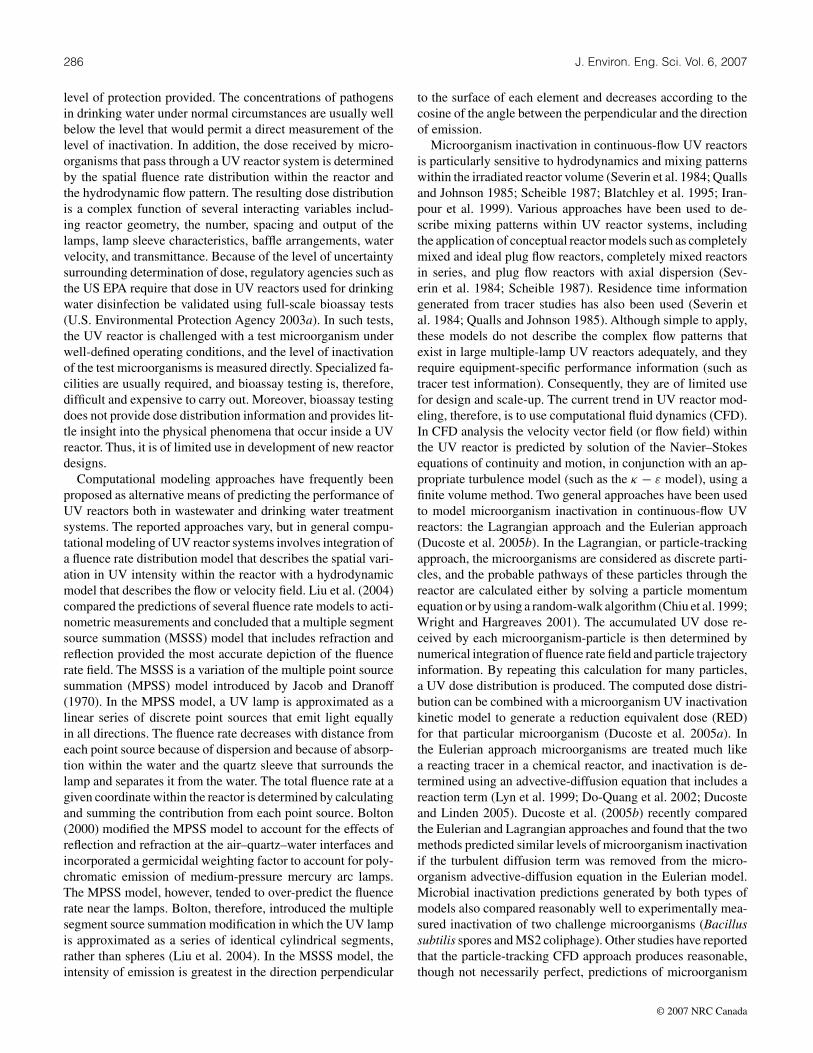
tegration of a number of distinct computational components,as illustrated in Fig. 2. The velocity field within the UV re-actor was computed using the FLUENT 6.1 (FLUENT INC.Lebanon, New Hampshire) commercial computational fluid dy-namics software package. This program applies a finite volumemethod to solve the Reynolds averaged Navier–Stokes (RANS)equations in conjunction with a turbulence model at discrete lo-cations within the physical domain. The computational meshesevaluated were produced using GAMBIT 2.0 software. The UVfluence field calculation and the microorganism inactivation ki-netics are user-defined functions that were combined with theCFD simulation. Relevant computational parameters for thebase-case simulation are summarized in Table 1.

Several computational meshes were evaluated, including bothfine and coarse and structured and unstructured hexahedralmeshes. Structured hexahedral meshes did not provide satisfac-tory convergence (normalized residuals of the continuity equa-tion >1 × 10−3). This was attributed to periodic flow oscilla-

Fig. 2. Flow sheet of the integrated UV reactor computationalmodel.

Velocity flow fieldRANS eqs. & turbulence

model (FLUENT 6.1)

Particle TrackingDPM & DRW models

UV dose distribution

Computation of the survivalratio of each particle, (N/N0)i ,

and overall inactivation,log10[1/nt Σ(N/N0)i]

UV fluence rate fieldMSSS Method

(UV Calc 3D-200)

Microorganism UVinactivation kinetics

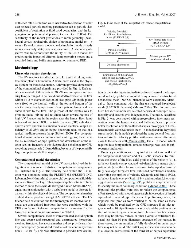
tion in the wake region immediately downstream of the lamps.Axial velocity profiles computed using a coarse unstructuredhexahedral mesh (583 521 elements) were essentially identi-cal to those computed with the fine unstructured hexahedralmesh (1 027 008 elements) (Munoz 2004). The fine unstruc-tured hexahedral mesh was selected because it converged satis-factorily and ensured grid independence. The mesh, describedin Fig. 3, was constructed with a progressively finer mesh res-olution nearer the lamps, walls, and baffle surfaces to providebetter resolution near these flow obstacles. Two types of turbu-lence models were evaluated: the κ −ε model and the Reynoldsstress model. Both models produced the same general flow pat-tern and similar velocity profiles, with some minor differencesclose to the reactor wall (Munoz 2004). The κ −ε model, whichrequired less computational time to converge, was used in sub-sequent simulations.

Boundary conditions were required at the inlet and outlet ofthe computational domain and at all solid surfaces. To mini-mize the length of the inlet, axial profiles of the velocity (ux,),turbulent kinetic energy (k), and turbulent kinetic energy dissi-pation rate (ε) at the inlet were assumed to be equal to those offully developed turbulent flow. Published correlations and datadescribing the profiles of velocity (Zagarola and Smits 1998),turbulent kinetic energy (Rodi 1984), and turbulent kinetic en-ergy dissipation rate (Versteeg 1995) profiles in a pipe were usedto specify the inlet boundary condition (Munoz 2004). Theseimposed inlet profiles were used to reduce the computationaleffort associated with modeling a straight inlet section of lengthequivalent to several pipe diameters. In preliminary work, theimposed inlet profiles were verified to be the same as thosewhich would be predicted by the CFD software if an inlet re-gion equal to 10 pipe diameters was used and the profiles at thestart of the inlet region were uniform. In some practical cases,there may be elbows, valves, or other hydraulic restrictions lo-cated less than 10 pipe diameters upstream of the reactor. Inthese cases, the assumption of fully developed turbulent pro-files may not be valid. The outlet y–z surface was chosen to beat a location downstream of the third set of baffles equivalent

© 2007 NRC Canada

Munoz et al. 289

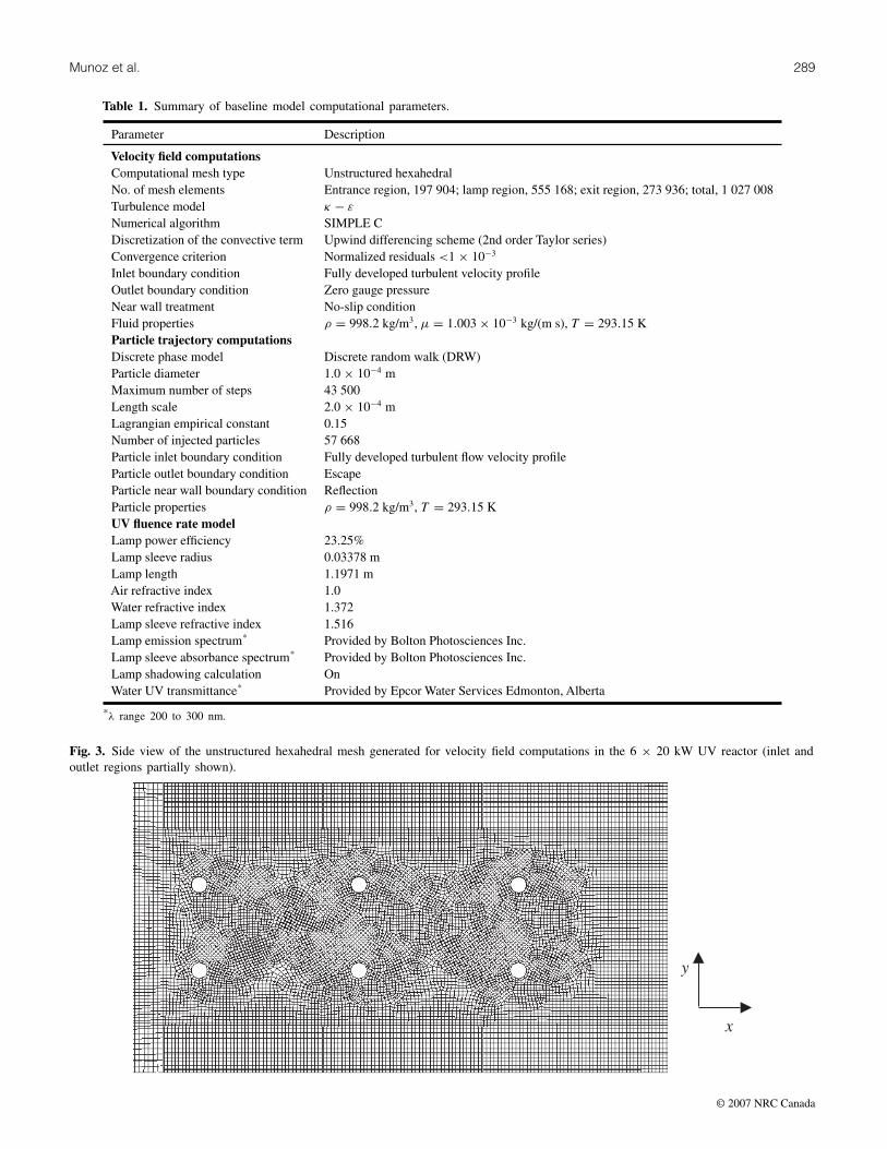
Table 1. Summary of baseline model computational parameters.

Parameter Description

Velocity field computationsComputational mesh type Unstructured hexahedralNo. of mesh elements Entrance region, 197 904; lamp region, 555 168; exit region, 273 936; total, 1 027 008Turbulence model κ − ε

Numerical algorithm SIMPLE CDiscretization of the convective term Upwind differencing scheme (2nd order Taylor series)Convergence criterion Normalized residuals <1 × 10−3

Inlet boundary condition Fully developed turbulent velocity profileOutlet boundary condition Zero gauge pressureNear wall treatment No-slip conditionFluid properties ρ = 998.2 kg/m3, µ = 1.003 × 10−3 kg/(m s), T = 293.15 KParticle trajectory computationsDiscrete phase model Discrete random walk (DRW)Particle diameter 1.0 × 10−4 mMaximum number of steps 43 500Length scale 2.0 × 10−4 mLagrangian empirical constant 0.15Number of injected particles 57 668Particle inlet boundary condition Fully developed turbulent flow velocity profileParticle outlet boundary condition EscapeParticle near wall boundary condition ReflectionParticle properties ρ = 998.2 kg/m3, T = 293.15 KUV fluence rate modelLamp power efficiency 23.25%Lamp sleeve radius 0.03378 mLamp length 1.1971 mAir refractive index 1.0Water refractive index 1.372Lamp sleeve refractive index 1.516Lamp emission spectrum* Provided by Bolton Photosciences Inc.Lamp sleeve absorbance spectrum* Provided by Bolton Photosciences Inc.Lamp shadowing calculation OnWater UV transmittance* Provided by Epcor Water Services Edmonton, Alberta

*λ range 200 to 300 nm.

Fig. 3. Side view of the unstructured hexahedral mesh generated for velocity field computations in the 6 × 20 kW UV reactor (inlet andoutlet regions partially shown).

y

x

© 2007 NRC Canada

290 J. Environ. Eng. Sci. Vol. 6, 2007

to at least 10 baffle heights. The pressure at the outlet was setequal to atmospheric pressure. The no-slip boundary conditionwas used at all internal surfaces (i.e., baffles, lamps, and reactorwalls).

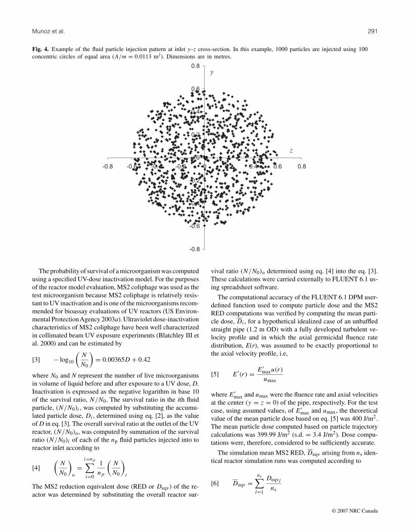
Microorganisms in the water entering the UV reactor wereconsidered to be contained within discrete spherical particlesof neutrally buoyant fluid. The trajectory of each fluid particlewas computed using the discrete phase model (DPM) subrou-tine in conjunction with a discrete random walk (DRW) model.A diameter of 1 × 10−4 m was chosen such that the fluid par-ticles were smaller than the smallest turbulent eddies yet muchlarger than a typical microorganism. The assumption was that10−4 m size fluid particles were small enough to capture the hy-drodynamic effects within the reactor while not being so smallas to unnecessarily prolong the simulations. Particle path stepsize must be dramatically reduced as particle size is reduced toaccurately simulate the individual particle paths. The densityof the particles was set equal to the density of the fluid (998kg/m3). In each particle trajectory simulation, a large number,np, of particles was introduced into the reactor inlet as follows.The inlet y-z reactor cross-section of area A was divided intom concentric rings of equal area A/m. The volumetric concen-tration of particles in each ring was set to a constant specifiedvalue cp = np/Q, where Q was the total volumetric flow rateentering the reactor. The volumetric flow rate in each concentricring j (j = 1, 2, , …, m) was approximated by integrating theturbulent axial velocity profile ux(r) according to

[1] Qj =rj+1∫rj

ux(r)2πr dr

where rj and rj+1 were the inside and outside radii of con-centric ring j, respectively. The number of particle additionpoints in each concentric ring was then determined accordingto nj = cpQj . The nj particle addition points were then ran-domly distributed across the surface of each concentric circle.This method produced an inlet injection particle injection pat-tern that was randomized with each simulation but weightedaccording to the turbulent velocity profile. An example patternis provided in Fig. 4. The “reflect” boundary condition, in whichthe normal and tangential coefficients of restitution are set equalto zero and one, was used at the wall. This minimizes the in-cidents of particles being trapped by the wall (velocity equalto zero) and being bounced off the wall (coefficient of restitu-tion = 1). The simulation was run until 98% of the particlesleft the computational domain. The maximum number of timesteps needed was 43 500.

The spatial UV fluence rate distribution was computed us-ing the UVCalc 3D-200 commercial program (Bolton Photo-sciences Inc., Edmonton, Alberta). This program uses the mul-tiple segment source summation (MSSS) method to calculatethe fluence rate, Eλ,xyz, at discrete x–y–z points in a multiplelamp UV reactor for each wavelength λ. In UVCalc 3D-200,each lamp is divided into a series of 1000 equally spaced cylin-drical segments. The contributions of each segment from eachof the six lamps were added to produce the UV fluence rate at

a given x–y–z coordinate within the reactor. The 3-D fluencerate field was generated by repeating this calculation for x–y–zcoordinates that matched the grid points of the fine unstruc-tured hexahedral mesh used in the velocity field calculations.The UVCalc 3D-200 model accounts for the UV absorbancespectrum of the water (between 200 and 300 nm), the spectraloutput of the medium-pressure lamps, reflection and refractionat the air–quartz and quartz–water interfaces, and the variationin intensity with angle of emission (Liu et al. 2004). Lampinput variables required for the UVCalc 3D-200 program, in-cluding the electrical output efficiency, emission spectrum ofthe medium-pressure lamp, and the absorbance spectrum of thequartz sleeve, were provided by Bolton Photosciences Inc. Thewater absorbance spectrum was based on a measurement ofthe absorbance spectrum of a sample of filtered drinking waterat the E.L. Smith drinking water treatment facility in Edmon-ton, Alberta, and was provided by EPCOR Water Services. Thetransmittance of the water at 254 nm for a 10 mm path lengthwas 95.91%. To simulate high and low transmittance, the trans-mittance at 254 nm was set to 93% and 80%, respectively, andthe transmittance at other wavelengths was reduced proportion-ately. Fluence rate calculations were computed at wavelengthintervals of 5 nm between 200 and 300 nm. The germicidaleffectiveness of each wavelength, λ, was weighted accordingto the absorbance spectrum of DNA to produce a germicidal-weighted fluence rate, E′

xyz, at each x–y–z coordinate (Bolton2000). This weighting assumes that the absorbance spectrum ofMS2 coliphage is similar to that of DNA. For the purposes ofthe sensitivity analysis presented in this study, lamp and sleevevariables, water absorbance spectrum, and the microorganismaction spectrum were assumed to be accurate. To make rigorouscompare of model predictions to experimental bioassay results,the modeler should verify the accuracy of these inputs by directmeasurement or by using rigorously validated information.

The UV dose distribution for each simulation was determinedby integrating the particle trajectory information produced byDPM with the fluence rate field information generated by UVCalc 3D-200. The accumulated UV dose received by a singleparticle, Di , was computed by summing the germicidal fluencerate along the path traveled by the particle through the UVreactor according to

[2] Di =t=tf∑t=0

E′t�t

where t is the Lagrangian time coordinate (the time of travel ofthe particle within the computational domain), �t is the com-putational time increment, and tf is the total simulation time.

Values of E′t determined using UV Calc 3D-200 served as in-

put into FLUENT 6.1. The particle dose, Di , for each injectedparticle was then computed within FLUENT 6.1 by specifyinga user-defined function in the DPM computational module. Toensure accurate computation of Di for each particle, a lengthscale of 2 × 10−4 m (equivalent to one half of the particle re-laxation time of 5.5 ×10−4 s) was used in the particle trajectorycomputations.

© 2007 NRC Canada

Munoz et al. 291

Fig. 4. Example of the fluid particle injection pattern at inlet y–z cross-section. In this example, 1000 particles are injected using 100concentric circles of equal area (A/m = 0.0113 m2). Dimensions are in metres.

-0.8

-0.6

-0.4

-0.2

0

0.2

0.4

0.6

0.8

-0.8 -0.6 -0.4 -0.2 0 0.2 0.4 0.6 0.8

y

z

The probability of survival of a microorganism was computedusing a specified UV-dose inactivation model. For the purposesof the reactor model evaluation, MS2 coliphage was used as thetest microorganism because MS2 coliphage is relatively resis-tant to UV inactivation and is one of the microorganisms recom-mended for bioassay evaluations of UV reactors (US Environ-mental ProtectionAgency 2003a). Ultraviolet dose-inactivationcharacteristics of MS2 coliphage have been well characterizedin collimated beam UV exposure experiments (Blatchley III etal. 2000) and can be estimated by

[3] − log10

(N

N0

)= 0.00365D + 0.42

where N0 and N represent the number of live microorganismsin volume of liquid before and after exposure to a UV dose, D.Inactivation is expressed as the negative logarithm in base 10of the survival ratio, N/N0. The survival ratio in the ith fluidparticle, (N/N0)i , was computed by substituting the accumu-lated particle dose, Di , determined using eq. [2], as the valueof D in eq. [3]. The overall survival ratio at the outlet of the UVreactor, (N/N0)o, was computed by summation of the survivalratio (N/N0)i of each of the np fluid particles injected into toreactor inlet according to

[4]

(N

N0

)o

=i=np∑i=0

1

np

(N

N0

)i

The MS2 reduction equivalent dose (RED or Deqv) of the re-actor was determined by substituting the overall reactor sur-

vival ratio (N/N0)o determined using eq. [4] into the eq. [3].These calculations were carried externally to FLUENT 6.1 us-ing spreadsheet software.

The computational accuracy of the FLUENT 6.1 DPM user-defined function used to compute particle dose and the MS2RED computations was verified by computing the mean parti-cle dose, Di , for a hypothetical idealized case of an unbaffledstraight pipe (1.2 m OD) with a fully developed turbulent ve-locity profile and in which the axial germicidal fluence ratedistribution, E(r), was assumed to be exactly proportional tothe axial velocity profile, i.e,

[5] E′(r) = E′maxu(r)

umax

where E′max and umax were the fluence rate and axial velocities

at the center (y = z = 0) of the pipe, respectively. For the testcase, using assumed values, of E′

max and umax, the theoreticalvalue of the mean particle dose based on eq. [5] was 400 J/m2.The mean particle dose computed based on particle trajectorycalculations was 399.99 J/m2 (s.d. = 3.4 J/m2). Dose compu-tations were, therefore, considered to be sufficiently accurate.

The simulation mean MS2 RED, Deqv arising from ns iden-tical reactor simulation runs was computed according to

[6] Deqv =ns∑

l=1

Deqvl

ns

© 2007 NRC Canada

292 J. Environ. Eng. Sci. Vol. 6, 2007

The standard deviation of Deqv was given by:

[7] SDeqv =√√√√ ns∑

l=1

Deqv2l− D

2eqv

ns − 1

The size of the 95% confidence interval on the mean MS2 REDwas computed using the student t-distribution according to

[8] EDeqv = tns−1,0.025SDeqv/√

ns

The theoretical UV dose, Dth, for each simulation was com-puted by assuming perfect plug flow (no dispersion) and com-plete radial mixing in the reactor. Under these idealized condi-tions, each particle would have the same residence time (ti =Q/V where V is the irradiated volume) and would be exposedto the same average fluence rate E′

avg where E′avg was the mean

of the E′xyz at each x–y–z location in the reactor. The reactor

hydraulic efficiency was defined as the ratio of the MS2 REDto the theoretical dose, ηH = Deqv/Dth.

Results and discussion

Base-case simulation resultsOne advantage of a computational fluid dynamic (CFD) ap-

proach to UV reactor modeling over conceptual models is that itpermits examination of the expected flow characteristics withinthe irradiated volume of the reactor. Computational fluid dy-namics can be used to identify potential regions of high localfluid velocity and by-pass flow, or regions of high recirculationthat may result in inefficient use of the reactor volume. An ex-ample of the computed flow field for the 6 × 20 kW reactor isprovided in Fig. 5. The operating conditions for the simulationof Fig. 4 are those of the base-case assumed for this study. Theseare (1) volumetric flowrate of 1.74 m3/s, which corresponds to amean superficial velocity of 1.54 m/s and a Reynolds number of1.83 × 106, (2) water UV transmittance (UVT) at 254 nm and10 mm path length of 93%, and (3) all six lamps in operation at100% electrical power with no lamp sleeve fouling. The spatialfluence rate distribution and the dose distribution for the basecase are provided in Figs. 6 and 7. The MS2 RED and inacti-vation predicted from the base cases simulation are 492 J/m2

and 2.2 log, respectively. These performance predictions are inthe range that would be expected for a typical drinking watertreatment facility.

The function of the baffles is to direct the water from lowfluence rate regions near the wall of the reactor towards thehigh fluence rate regions in the vicinity of the lamps. This pro-motes cross-mixing across the fluence rate gradients, whichtends to result in a narrower dose distribution and improveddisinfection. The flow simulations also show that the bafflesresult in high-velocity regions near the center of the reactorand low-velocity regions near the reactor walls (Fig. 5). Thelow-velocity recirculation regions downstream of the bafflesresult in the long asymmetric tail of the dose distribution athigher doses (Fig. 7). Although the MS2 RED for the base-casesimulation was 492 W/m2, approximately 13% of the particles

received doses in the 250 to 350 W/m2 range (Fig. 7). However,few particles received UV doses of less than 250 W/m2, sug-gesting that there was very little short-circuiting through zonesof low fluence rate. Although this flow pattern prevents poorinactivation due to short-circuiting, it results in an effective ex-posure time that is much less than the theoretical exposure timebased on the superficial mean velocity. The local velocities inthe central region are almost twice the mean superficial velocityof 1.54 m/s, and the hydrodynamic efficiency is ηH = 0.55.

Evaluation of particle injection criteriaWhen the discrete random walk (DRW) is used to calculate

particle trajectories in DPM, the predictions of dose distribu-tion, microorganism inactivation, and RED will differ with eachsimulation owing to the random particle velocity componentsinherent in the model. For example, Fig. 8 shows three differ-ent particle trajectories calculated for particles injected at thesame inlet point for three different simulations. As indicated inthe figure, these particles follow entirely different trajectoriesand have different accumulated UV doses. The statistical sig-nificance of a simulation result can be improved by increasingthe total number of particles used in each simulation, np. Useof too few particles will result in low reproducibility, poor ac-curacy and low statistical insignificance. Use of an excessivelylarge number of particles, on the other hand, results in unneces-sary computational effort and data file sizes. The modeler mustselect the value of np with care.

Graham and Moyeed (2002) proposed an efficient method todetermine the number of particles that are needed to produceresults within certain defined confidence limits in Lagrangiansimulations. A similar approach was adopted in this study fordetermining an appropriate value of np for simulating micro-organism inactivation in the 6 × 20 kW UV reactor. Two sets ofreplicated particle tracking simulations were run using DPM inconjunction with the DRW model as follows. In the first set, thetotal number of simulations, ns, was kept constant at 30 while npwas varied. In the second, np was held constant at 1000, while nswas varied. When the magnitude of the 95% confidence inter-val computed using eq. [8] was plotted against the total numberof particles used in all simulations npns, the variability in thecomputed inactivation was found to be inversely proportionalto npns (Fig. 9). This is consistent with the findings of Grahamand Moyeed (2002) who reported that variability was propor-tional to {1/(npns)

0.5} for simulation of particle-laden air flowsin ducts. At npns less than approximately 20 000, the computedMS2 RED was sensitive to both the product npns and the valuesof np and ns. For given value of npns in this range, the variabil-ity was lower and the reproducibility was better, when moresimulations were used with fewer particles per simulation. Asnpns increased to greater than 30 000 particles, the variationstabilized at approximately 2.0 J/m2 and was independent ofthe values of np and ns. This variation is less than 1% of the re-duction MS2 RED of 492 J/m2 and is an acceptable uncertaintyrelative to the expected uncertainty for bioassay results. Thisfinding implies that at sufficiently high npns (i.e., >30 000),similar variability can be expected using one simulation with

© 2007 NRC Canada

Munoz et al. 293

Fig. 5. Velocity magnitude contours in the 6 × 20 kW reactor for the base-case CFD simulation. The view is in a vertical x–y planewith z = 0.

Fig. 6. Fluence rate distribution for the 6 × 20 kW reactor for the base-case fluence simulation. The view is in a vertical x–y plane withz = 0. Germicidal fluence rates, E′

xyz, are given in W/m2.

30 000 particles or 10 simulations with 3 000 particles each.This is of significance to the modeler because it is generallymore convenient to run a single simulation with a large num-ber of particles rather than several simulations with a smallnumber of particles. The results of these simulations suggest

that, for the 6 × 20 kW UV reactor, single simulations using30 000 or more particles will produce satisfactory precision.In general, the optimum number of particles will depend onsystem specific variables such as reactor geometry, flow rate,water UV absorbance, lamp characteristics, and UV resistance

© 2007 NRC Canada

294 J. Environ. Eng. Sci. Vol. 6, 2007

Fig. 7. Dose distribution computed for the base-case simulation with np = 57 668. Computed equivalent dose is Deqv = 492 J/m2.

0

5

10

15

20

25

30

35

40

<20

0

300

500

700

900

1100

1300

1500

1700

190

0

2100

230

0

250

0

270

0

290

0

>30

00

Particle Dose, Di (J/m2)

Rel

ativ

efr

equ

ency

(%)

Deqv

Fig. 8. Example of trajectories computed in separate simulations for three fluid particles released at the same location at the inlet of theUV reactor computational domain. Colors indicate accumulated UV fluence in mJ/cm2.

of the particular microorganism under consideration. Althoughthe exercise described above will provide some general guid-ance, a similar particle number study should be carried out forspecific UV reactor systems to ensure a stable solution.

Evaluation of the Lagrangian empirical constant, CLThe computational modeler must select an appropriate model

to describe the interaction between the dispersed phase (i.e.,the particles) and the continuous phase (i.e., carrier fluid) when

carrying out particle trajectory simulations. In this study, thediscrete-random walk (DRW) model was used to describe thisinteraction. When using the DRW model, the modeler mustspecify a value for the Lagrangian time constant, CL. This em-pirical constant is related to the time period that a particle isallowed to interact with an eddy in turbulent flow. The valueof CL determines the degree of particle dispersion within thecarrier fluid and may have an important influence on the com-puted inactivation and MS2 RED in a UV reactor. MacInnes and

© 2007 NRC Canada

Munoz et al. 295

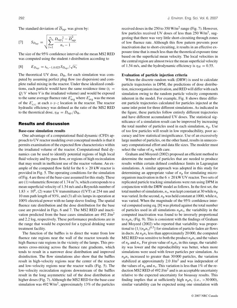
Fig. 9. Size of the confidence interval on equivalent dose, EDeqv , as a function of the total number of particles (np × ns) for two sets ofsimulations. Base-case simulation conditions (Table 1) were used.

E Deqv = 329.92(n p x n s)-0.49

r2

= 0.8999

E Deqv = 1335.1(n p x n s)-0.62

r2

= 0.9738

0

1

2

3

4

5

6

7

8

0 10 000 20 000 30 000 40 000 50 000 60 000

n p x n s

ED

eqv(J

/m2 )

ns = 30, np variable (simulations)np = 1000, ns variable (simulations)ns = 30, np variable (curve fit)np = 1000, ns variable (curve fit)

Table 2. Matrix of experimental simulations used to determine the effect of the Lagrangian empirical constant on UV reactorperformance predictions.

Simulation input Simulation outputs

Run NLO � (kW) Q (m3/s) EED (kW h/m3) UVT (%) CL Dth (J/m2) -log10 (N/N0) Deqv (J/m2) ηH

1* + + + + + - 900.8 2.22 492.2 0.5462 + + + + + + 900.8 2.26 505.3 0.5613 + + + + - - 310.5 0.84 113.9 0.3674 + + + + - + 310.5 0.86 120.5 0.3885 - + - - + - 600.0 1.73 359.1 0.5986 - + - - + + 600.0 1.74 362.5 0.6047 - + - - - - 206.8 0.74 86.3 0.4178 - + - - - + 206.8 0.74 86.7 0.4199 + - - - + - 594.0 1.711 353.7 0.595

10 + - - - + + 594.0 1.749 364.1 0.61311 + - - - - - 204.7 0.743 88.4 0.43212 + - - - - + 204.7 0.760 93.3 0.455

Note: Experimental input ranges: NLO, lamps 1 and 2 (-) or all 6 (+) lamps; �, 6.7 (-) or 20 (+) kW Q, 0.87 (-) or 1.74 (+) m3/s; EED,0.0128 (-) or 0.0192 (+) kW h/m3; UVT, 80% (-) or 93% (+) at 254 nm and 10 mm; CL: 0.15 (-) or 0.30 (+).*Base-case simulation.

Bracco (1992) found there was little consensus in the literatureon values of the Lagrangian time constant used in homogeneousturbulent flow models, with reported values ranging from 0.06to 0.63. It was of some interest, therefore, to determine the sen-sitivity of predicted inactivation and RED to the value of theLagrangian time constant in the DRW model.

The effect of reducing the Lagrangian empirical constantfrom 0.30 to 0.15 (the values recommended by FLUENT 6.1for use with the DRW model) was determined at various low

(–) and high (+) combinations of electrical energy dose (EED)and UV transmittance of the water (UVT). Conditions for thesimulations and corresponding simulation results are providedin Table 2. The electrical energy dose, EED, was determinedby the number of lamps in operation NLO), individual lamppower (�), and flow rate (EED = NLO × �/Q) and is a mea-sure of the energy input per volume of water treated. The highEED condition (0.0192 kW h/m3) was specified by setting allsix lamps to 100% power with the water flow rate at a low

© 2007 NRC Canada

296 J. Environ. Eng. Sci. Vol. 6, 2007

Table 3. Least-squares coefficients of regression modelrelating predictions of equivalent dose, electrical energydose, water UV transmittance and Lagrangian empiricalconstant.

Coefficient Input Coefficients P-value

α0 Intercept 266.1α1 EED 41.9 1.3 × 10−9

α2 UVT 163.2 9.4 × 10−14

α3 CL 3.2 0.012α12 UVT × EED 27.6 2.3 × 10−8

Reduced Model: Deqv = α0 + α1(EED) + α2(UVT) + α3(CL)+ α12(EED × UVT)

level (0.87 m3/s) (simulation runs 1–4). The low EED condi-tion (0.0128 kW h/m3) was specified in two low flow operatingmodes: with all six lamps in operation at 33% power each (sim-ulation runs 5–8) or with 2 lamps in operation (lamps 1 and 2 asshown in Fig. 1) at 100% power each (simulation runs 9–12).These operating conditions were chosen to reflect a wide rangeof operating conditions that would be encountered in operationof this type of UV reactor in a water treatment plant.

Least-squares linear regression was used to further examinethe effects of the inputs (EED, UVT, and CL) and their interac-tions on MS2 RED, Deqv. As expected, the reduced regressionmodel (Table 3), indicates that EED, UVT, and the interactionEED × UVT had statistically significant effects on the MS2RED (i.e., the associated p-value was less than 0.05). The valueof the Lagrangian time constant, CL, was determined to havea statistically significant effect on dose (p-value = 0.012). Onaverage, decreasing the value of CL from 0.30 to 0.15 corre-sponded to a reduction in the predicted MS2 RED of 6.5 J/cm2,which is only 1.2% of the average computed MS2 RED. Al-though statistically significant, this effect may be practicallyunimportant. The interactions between CL and EED or UVTwere not statistically significant, which suggests that the mag-nitude of the CL effect can be expected to be essentially fixedover the normal UV reactor operating range. Use of the de-fault values of CL provided by FLUENT 6.1 should providereasonably accurate dose predictions for large UV reactors.

Evaluation of mesh geometry, turbulence model andunsteady flow

Numerous other computational parameters must be selectedby the modeler when carrying out CFD simulations of large UVreactors.Additional simulations were carried out to examine theeffect of selected computational parameters (mesh geometry,type of turbulence model, and simulation mode) on computedMS2 RED in the 6 × 20 kW reactor including. Each parame-ter was varied independently, and the resulting computed MS2RED was compared with that of the base case (492 J/m2). Re-sults are provided in Table 4.

The unstructured tetrahedral mesh is more easily and readilygenerated than the unstructured hexahedral mesh that was usedin the base case. This advantage, however, may be offset by adecrease in the accuracy of the predictions. Selection of an un-structured tetrahedral mesh versus the unstructured hexahedral

mesh resulted in a 7% increase in computed MS2 RED eventhough 22% more mesh elements were used for the unstructuredtetrahedral mesh to ensure the same level of grid independence.The unstructured tetrahedral mesh was found to predict lowervelocities in the central region of the reactor when comparedwith the unstructured hexahedral mesh (data not shown). Thisis consistent with higher predicted microorganism average res-idence time, MS2 inactivation, and RED. Under-prediction ofvelocity will consistently over-predict dose, so modelers shoulduse tetrahedral meshes with caution when simulating large UVreactors.

In most reported studies on CFD modeling of UV reactors,the κ − ε model has been used as the turbulence model, i.e.,Blatchley et al. (1998); Lyn et al. (1999). The Reynolds stressmodel (RSM), an alternative to the κ −ε model, should providea better description of nonhomogeneous flows because it solvesfor each component of the Reynolds stresses rather than the totalkinetic energy (Wright and Hargreaves 2001). The differencein the predicted MS2 RED generated using the two turbulencemodels (κ − ε and RSM) was less than 4%. A higher orderturbulence model may be needed only if a very high level ofprecision is required. Depending on the level of accuracy de-sired, modelers should, therefore, make the choice of turbulencemodel carefully.

Typically, UV reactor simulations are done in steady-statemode. In reality, the velocity field within a UV reactor changeswith time as large eddies expand and collapse. The unsteady-state simulation feature of FLUENT 6.1 was used to predictthe impact of these transient characteristics on computed in-activation. Although the unsteady-state state simulations pro-vided interesting information regarding transient flow phenom-ena within the reactor, such as the generation and collapse ofeddies downstream of the baffles and lamps, the computed in-activation and MS2 RED changed by less than 2% from thesteady-state simulation. The steady-state simulation was, there-fore, considered adequate for modeling of this large UV reactor.

Evaluation of lamp operation modeComputational fluid dynamics modeling may be used to pre-

dict the influence of different operating modes on UV reactorperformance and to assist in determining the most efficient orcost-effective operating strategies for changing water flow orquality conditions. For example, at a given flow rate, the de-sired electrical energy dose may be achieved by controlling ei-ther the number of lamps in operation or the power to each lamp.In simulation runs 5 to 12 in Table 2, the EED was maintainedat 0.0128 kW h/m3for a flow rate of 0.87 m3/s by operating witheither lamps 1 and 2 (Fig. 1) both at 100% power, or with all sixlamps in operation, each at 33% power. A regression analysisrevealed that the effect on computed MS2 RED and hydraulicefficiency was not statistically significant. In this case, the de-cision to operate the reactor in either mode should be based onconsiderations such as optimizing lamp life. If only two lampsare used, however, the efficiency may depend on which two ofthe six lamps are in operation. Table 5 shows the results of a setof simulations in which different pairs of lamps were operated

© 2007 NRC Canada

Munoz et al. 297

Table 4. Effect of additional computational parameters on computed equivalent dose.

Run Mesh type Turbulence model Simulation mode -log10 (N/N0) Deqv (J/m2)

1* Hexahedral κ − ε Steady state 2.21 492.713 Tetrahedral κ − ε Steady state 2.34 527.714 Hexahedral RSM Steady state 2.15 475.315 Hexahedral κ − ε Unsteady state 2.19 485.4

Note: RSM, Reynolds stress model.*Base-case simulation.

Table 5. Effect of various combinations of lamp operation on predicted UVreactor performance.

Run NLO∗ CL Dth (J/m2) -log10 (N/N0) Deqv (J/m2) ηH

5 1, 2 0.15 600.0 1.731 359.1 0.5986 1, 2 0.30 600.0 1.743 362.5 0.6045b 1, 4 0.15 608.8 1.645 335.6 0.5586b 1, 4 0.30 608.8 1.644 335.2 0.5585c 1, 6 0.15 600.6 1.612 326.7 0.5446c 1, 6 0.15 600.6 1.591 320.8 0.534

Note: Operating conditions: � = 20 kW, Q = 0.84 m3/s, EED = 0.0128 kW h/m3,UVT = 93% at 254 nm at 10 mm path length.∗Lamp numbers shown in Fig. 1.

at identical flow, EED, and UVT conditions. The greatest hy-draulic efficiency and MS2 RED were achieved when the twolamps in operation were selected from the same vertical bank.Operation of the two lamps in different vertical banks increasesthe probability that a microorganism travels only through re-gions of low fluence rate and bypasses regions of high fluence.The vertical banks are hydraulically equivalent, so the bankchosen will not affect the Deqv.

Evaluation of a modified ultraviolet reactor designComputational fluid dynamics in conjunction with fluence

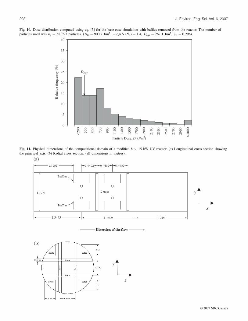
rate modeling can be used to examine the effect of design vari-ables and modifications on UV reactor performance and to aidin the development of new reactor designs. The dose distribu-tion computed for the 6 × 20 kW reactor with baffles removed(Fig. 10) was much broader than the one computed for the reac-tor with baffles in place (Fig. 7). Most significantly, many moreparticles received a low UV dose ( <250 J/m2) when the baf-fles were removed resulting in a considerable reduction in MS2coliphage inactivation (1.40 vs. 2.22), RED (267 vs. 492 J/m2),and hydraulic efficiency (0.296 vs. 0.546). Baffles are impor-tant for ensuring appropriate mixing across fluence rate gradi-ents and good hydraulic efficiency; however, they also increasehydraulic pressure drop across the reactor.

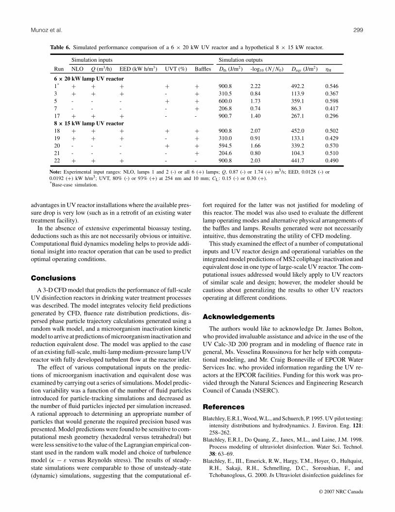
Figure 11 describes a hypothetical 8 × 15 kW modified reac-tor design. In this reactor, eight 15 kW medium-pressure lampswere arranged perpendicular to the bulk flow and perpendicularto each other. The modified reactor contained 16 small bafflesoriented perpendicular to the flow. Although there were morebaffles, the total baffle area was considerably less than that ofthe 6 × 20 kW reactor. The lamp and baffle arrangement in the

modified reactor was selected because it is expected to provide abetter spatial distribution of the fluence rate with lower pressuredrop in comparison to the 6 × 20kW UV reactor. Disadvantagesof the design are that the lamp arrangement may make it dif-ficult to remove some lamps for maintenance or replacementand the extra two lamps will demand additional monitoring andmechanical cleaning systems.

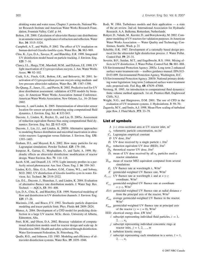
Simulations were carried out with the modified reactor designat various sets of operating conditions. The simulation resultsare compared with a similar set of simulations on the original6 × 20 kW reactor in Table 6. The predicted hydraulic efficiencyfor the 8 × 15 kW UV reactor was 4% percent less than that ofthe 6 × 20 kW UV reactor when the water UV transmittancewas high (compare runs 1 and 5 with 18 and 20). On the otherhand, the predicted hydraulic efficiency for the 8 × 15 kW UVreactor was 6%–10% greater than that of the 6 × 20 kW UVreactor at low UV transmittance (compare runs 3 and 7 with19 and 21). The simulation results indicate that the benefit ofthe modified reactor design only appears in low transmittancewater.

Baffles played a much less important role in the modified8 × 15 kW UV reactor than in the 6 × 30 kW reactor. Removalof baffles in the 6 × 20 kW reactor resulted in a reduction ofhydraulic efficiency from 0.546 to 0.296 (runs 1 and 17). Forthe modified 8 × 20 kW reactor, removal of the baffles resultedin a reduction in hydraulic efficiency from 0.502 to 0.490 (runs18 and 22). The pressure drops predicted by FLUENT 6.1 forthe 6 × 20 kW UV reactor, with and without baffles, were 3 and1 kPa, respectively. For the 8 × 15 kW UV reactor, the predictedpressure drops, with and without baffles, were 1.8 and 1.2 kPa,respectively. The modified reactor design may have important

© 2007 NRC Canada

298 J. Environ. Eng. Sci. Vol. 6, 2007

Fig. 10. Dose distribution computed using eq. [3] for the base-case simulation with baffles removed from the reactor. The number ofparticles used was np = 58 397 particles. (Dth = 900.7 J/m2, −log(N/N0) = 1.4, Deqv = 267.1 J/m2, ηH = 0.296).

0

5

10

15

20

25

30

35

40

<20

0

300

500

700

900

110

0

130

0

150

0

170

0

190

0

2100

2300

2500

2700

2900

>3

000

Particle Dose, (J/mDi2)

Rel

ativ

efr

equ

ency

(%)

Deqv

Fig. 11. Physical dimensions of the computational domain of a modified 8 × 15 kW UV reactor. (a) Longitudinal cross section showingthe principal axis. (b) Radial cross section. (all dimensions in metres).

© 2007 NRC Canada

Munoz et al. 299

Table 6. Simulated performance comparison of a 6 × 20 kW UV reactor and a hypothetical 8 × 15 kW reactor.

Simulation inputs Simulation outputs

Run NLO Q (m3/h) EED (kW h/m3) UVT (%) Baffles Dth (J/m2) -log10 (N/N0) Deqv (J/m2) ηH

6 × 20 kW lamp UV reactor1* + + + + + 900.8 2.22 492.2 0.5463 + + + - + 310.5 0.84 113.9 0.3675 - - - + + 600.0 1.73 359.1 0.5987 - - - - + 206.8 0.74 86.3 0.41717 + + + - - 900.7 1.40 267.1 0.2968 × 15 kW lamp UV reactor18 + + + + + 900.8 2.07 452.0 0.50219 + + + - + 310.0 0.91 133.1 0.42920 - - - + + 594.5 1.66 339.2 0.57021 - - - - + 204.6 0.80 104.3 0.51022 + + + - - 900.8 2.03 441.7 0.490

Note: Experimental input ranges: NLO, lamps 1 and 2 (-) or all 6 (+) lamps; Q, 0.87 (-) or 1.74 (+) m3/s; EED, 0.0128 (-) or0.0192 (+) kW h/m3; UVT, 80% (-) or 93% (+) at 254 nm and 10 mm; CL: 0.15 (-) or 0.30 (+).*Base-case simulation.

advantages in UV reactor installations where the available pres-sure drop is very low (such as in a retrofit of an existing watertreatment facility).

In the absence of extensive experimental bioassay testing,deductions such as this are not necessarily obvious or intuitive.Computational fluid dynamics modeling helps to provide addi-tional insight into reactor operation that can be used to predictoptimal operating conditions.

Conclusions

A 3-D CFD model that predicts the performance of full-scaleUV disinfection reactors in drinking water treatment processeswas described. The model integrates velocity field predictionsgenerated by CFD, fluence rate distribution predictions, dis-persed phase particle trajectory calculations generated using arandom walk model, and a microorganism inactivation kineticmodel to arrive at predictions of microorganism inactivation andreduction equivalent dose. The model was applied to the caseof an existing full-scale, multi-lamp medium-pressure lamp UVreactor with fully developed turbulent flow at the reactor inlet.

The effect of various computational inputs on the predic-tions of microorganism inactivation and equivalent dose wasexamined by carrying out a series of simulations. Model predic-tion variability was a function of the number of fluid particlesintroduced for particle-tracking simulations and decreased asthe number of fluid particles injected per simulation increased.A rational approach to determining an appropriate number ofparticles that would generate the required precision based waspresented. Model predictions were found to be sensitive to com-putational mesh geometry (hexadedral versus tetrahedral) butwere less sensitive to the value of the Lagrangian empirical con-stant used in the random walk model and choice of turbulencemodel (κ − ε versus Reynolds stress). The results of steady-state simulations were comparable to those of unsteady-state(dynamic) simulations, suggesting that the computational ef-

fort required for the latter was not justified for modeling ofthis reactor. The model was also used to evaluate the differentlamp operating modes and alternative physical arrangements ofthe baffles and lamps. Results generated were not necessarilyintuitive, thus demonstrating the utility of CFD modeling.

This study examined the effect of a number of computationalinputs and UV reactor design and operational variables on theintegrated model predictions of MS2 coliphage inactivation andequivalent dose in one type of large-scale UV reactor. The com-putational issues addressed would likely apply to UV reactorsof similar scale and design; however, the modeler should becautious about generalizing the results to other UV reactorsoperating at different conditions.

Acknowledgements

The authors would like to acknowledge Dr. James Bolton,who provided invaluable assistance and advice in the use of theUV Calc-3D 200 program and in modeling of fluence rate ingeneral, Ms. Vesselina Roussinova for her help with computa-tional modeling, and Mr. Craig Bonneville of EPCOR WaterServices Inc. who provided information regarding the UV re-actors at the EPCOR facilities. Funding for this work was pro-vided through the Natural Sciences and Engineering ResearchCouncil of Canada (NSERC).

References

Blatchley, E.R.I., Wood, W.L., and Schuerch, P. 1995. UV pilot testing:intensity distributions and hydrodynamics. J. Environ. Eng. 121:258–262.

Blatchley, E.R.I., Do Quang, Z., Janex, M.L., and Laine, J.M. 1998.Process modeling of ultraviolet disinfection. Water Sci. Technol.38: 63–69.

Blatchley, E., III., Emerick, R.W., Hargy, T.M., Hoyer, O., Hultquist,R.H., Sakaji, R.H., Schmelling, D.C., Soroushian, F., andTchobanoglous, G. 2000. In Ultraviolet disinfection guidelines for

© 2007 NRC Canada

300 J. Environ. Eng. Sci. Vol. 6, 2007

drinking water and water reuse, Chapter 3: protocols. National Wa-ter Research Institute and American Water Works Research Foun-dation, Fountain Valley, Calif. p. 64.

Bolton, J.R. 2000. Calculation of ultraviolet fluence rate distributionsin an annular reactor: significance of refraction and reflection. WaterRes. 34: 3315–3324.

Campbell, A.T., and Wallis, P. 2002. The effect of UV irradiation onhuman-derived Giardia lamblia cysts. Water Res. 36: 963–969.

Chiu, K., Lyn, D.A., Savoye, P., and Blatchley, E.R. 1999. IntegratedUV disinfection model based on particle tracking. J. Environ. Eng.125: 7–16.

Clancy, J.L., Hargy, T.M., Marshall, M.M., and Dyksen, J.E. 1998. UVlight inactivation of Cryptosporidium oocysts. J. Am. Water WorksAssoc. 90: 92–102.

Craik, S.A., Finch, G.R., Bolton, J.R., and Belosevic, M. 2001. In-activation of Cryptosporidium parvum oocysts using medium- andlow-pressure ultraviolet radiation. Water Res. 35: 1387–1398.

Do-Quang, Z., Janex, J.L., and Perrin, R. 2002. Predictive tool for UVdose distribution assessment: validation of CFD models by bioas-says. In American Water Works Association Annual Conference.American Water Works Association, New Orleans, La., 16–20 June2002.

Ducoste, J., and Linden, K. 2005. Determination of ultraviolet sensorlocation for sensor set-point monitoring using computational fluiddynamics. J. Environ. Eng. Sci. 4: S33-S43.

Ducoste, J., Linden, K., Royker, D., and Liu, D. 2005a. Assessmentof reduction equivalent fluence bias using computational fluid dy-namics. Environ. Eng. Sci. 22: 615–628.

Ducoste, J., Liu, J.J., and Linden, K. 2005b. Alternative approachesto modeling fluence distribution and microbial inactivation in ultra-violet reactors: Lagrangian versus Eulerian. J. Environ. Eng. 131:1393–1403.

Graham, D.I., and Moyeed, R.A. 2002. How many particles for myLagrangian simulations. Powder Technol. 125: 179–186.

Iranpour, R., Garnas, G., Moghaddam, O., and Taebi, A. 1999. Hy-draulic effects an ultraviolet disinfection: modification of reactordesign. Water Environ. Res. 71: 114–118.

Jacob, S.M., and Dranoff, J.S. 1970. Light intensity profiles in a per-fectly mixed photoreactor. Am. Inst. Chem. Eng. J. 16: 359–363.

Linden, K.G., Shin, G.A., Faubert, G.M., Cairns, W.L., and Sobsey,M.D. 2002. UV disinfection of Giardia lamblia cysts in water. En-viron. Sci. Technol. 36: 2519–2522.

Liu, D.L., Ducoste, J., Shanshan, J., and Linden, K. 2004. Evaluationof alternative fluence rate distribution models. J. Water Sup. Res.Technol. — AQUA, 53: 391–408.

Lyn, D.A., Chiu, K., and Blatchley, E.R. 1999. Numerical modeling offlow and disinfection in UV disinfection channels. J. Environ. Eng.125: 17–26.

Macinnis, J.M., and Braco, F.V. 1992. Stochastic particle dispersionmodeling and tracer particle limit. Phys. Fluids A4: 2809–2824.

Munoz, A. 2004. Development of a CFD model for predicting disin-fection in a large UV reactor. M.Sc. thesis. University of Alberta,Edmonton, Alta.

Petri, B.M., and Olson, D.A. 2002. Bioassay validation of computa-tional disinfection models used for reactor design and scale-up. InDisinfection 2002: Health and safety achieved through disinfection.Water Environment Federation, St. Petersburg, Fla.

Qualls, R.G., and Johnson, J.D. 1985. Modeling and efficiency of ul-traviolet disinfection systems. Water Res. 19: 1039–1046.

Rodi, W. 1984. Turbulence models and their application — a stateof the art review. 2nd ed. International Association for HydraulicResearch. A.A. Balkema, Rotterdam, Netherlands.

Rokyer, D., Valade, M., Keesler, D., and Borsykowsky, M. 2002. Com-puter modeling of UV reactors for validation purposes. InAmericanWater Works Association — Water Quality and Technology Con-ference, Seattle, Wash. p. 21

Scheible, O.K. 1987. Development of a rationally based design pro-tocol for the ultraviolet light disinfection process. J. Water Pollut.Control Fed. 59: 25–31.

Severin, B.F., Suidan, M.T., and Engelbrecht, R.S. 1984. Mixing ef-fects in UV disinfection. J. Water Pollut. Control Fed. 56: 881–888.

US Environmental Protection Agency. 2003a. Long term 2 enhancedsurface water treatment rule — toolbox guidance manual. EPA 815-D-03-009. Environmental Protection Agency, Washington, D.C.

US Environmental Protection Agency. 2003b. National primary drink-ing water legislation: long term 2 enhanced surface water treatmentrule; proposed rule. Fed. Reg. 68: 47639–47688.

Versteeg, H. 1995. An introduction to computational fluid dynamics:finite volume method approach. 1st ed. Prentice-Hall, EnglewoodCliffs, N.J.

Wright, N.G., and Hargreaves, D.M. 2001. The use of CFD in theevaluation of UV treatment systems. J. Hydroinform. 3: 59–70.

Zagarola, M.V., and Smits, A.J. 1998. Mean-Flow scaling of turbulentpipe flow. J. Fluid Mech. 373: 33–79.

List of symbols

A y–z cross-sectional area at UV reactor inlet, m2

cp volumetric particle concentration, no./m3

CL Lagrangian empirical constantD UV dose, J/m2

Di UV dose received by a single particle i, J/m2

Deqv reduction equivalent UV dose (RED), J/m2

Dth theoretical reactor UV dose, J/m2

Di mean of UV dose received by all np particles used areactor simulation

Deqv mean of reactor MS2 equivalent computed from severalsimulations

Eλ UV fluence rate at wavelength λ, W/m2

E′ germicidal-weighted UV fluence rate, W/m2

Eλ,xyz UV fluence rate at wavelength λ and at x–y–zcoordinate, W/m2

E′xyz germicidal-weighted UV fluence rate at coordinate

x–y–z, W/m2

E(r) germicidal-weighted UV fluence rate at radial distance rfrom the principal axis of the reactor, W/m2

E′avg average germicidal-weighted UV fluence in the reactor,

W/m2

E′max germicidial-weighted UV fluence rate at principal axis

of the reactor (y = z = 0), W/m2

EED electrical energy dose, kW h/m3

i subscript representing individual fluid particles, i = 1,2, …, np

j subscript representing individual concentric rings atreactor inlet, j = 1, 2, …, m

k turbulent kinetic energyl subscript representing each simulation in a series, l = 1,

2, …, ns

© 2007 NRC Canada

Munoz et al. 301

nj number of fluid particles added to concentric ringk

np total number of fluid particles injected per simula-tion

ns number of simulationsN number or concentration of live organisms after

exposure to UV lightN0 number or concentration of live organisms prior to

exposure to UV lightN/N0 survival ratio

(N/N0)i survival ratio in fluid particle i(N/N0)o overall survival ratio at the outlet of the reactor

NLO number of lamps in operationp-value probability of a type I error

Q volumetric flow rate, m3/sQj approximate volumetric flow rate into jth concen-

tric ring at reactor inlet, m3/sr radial distance from principal axis of the reactor,

mt Lagrangian time coordinate, stf total simulation time, sti residence time of particle i, s

�t Lagrangian time interval in discrete phase modelcalculations, s

tns ,−1,0.025 Student t-statistic

T fluid temperature, Kux axial velocity, m/s

ux(r) axial velocity at radial distance r from principalaxis of reactor, m/s

umax axial velocity at principal axis of the reactor(y = z = r = 0), m/s

SDeqv standard deviation of the MS2 reduction equiv-alent dose computed from repeated simulations,W/m2

V irradiated volume, m3

x Cartesian coordinate in direction parallel tomain water flow

y Cartesian coordinate in direction perpendicularto lamps and main water flow

z Cartesian coordinate in direction parallel to axisof UV lamps

α0, α1, α2, α3, α12 least-squares regression coefficientsε dissipation rate of turbulent kinetic energy,

m2/s3

ηH hydraulic efficiencyλ wavelength, nmµ fluid viscosity, kg/ (m s)ρ fluid or particle density, kg/m3

� power output per lamp, kW

© 2007 NRC Canada