Chapter 56

Lattice Boltzmann Method for Computational FluidDynamics

Li-Shi Luo1, Manfred Krafczyk2, and Wei Shyy31 Department of Mathematics & Statistics and Center for Computational Sciences, Old Dominion University, Norfolk, USA2 Institute for Computational Modeling in Civil Engineering, Technische Universitat Braunschweig, Braunschweig,Germany3 Department of Aerospace Engineering, University of Michigan, Ann Arbor, MI, USA

1 Theory of The Lattice Boltzmann Equation 651

2 Applications in Computational Fluid Dynamics 654

3 Conclusions and Outlook 658

Acknowledgments 659

References 659

1 THEORY OF THE LATTICEBOLTZMANN EQUATION

The lattice Boltzmann equation (LBE) was proposed morethan twenty years ago as a successor to the lattice-gas cellu-lar automata (LGCA) as a model for hydrodynamic systems.Both the LGCA and the LBE are based on microscopic anddiscrete descriptions of fluids, as opposed to macroscopicand continuum descriptions, which are the theoretical foun-dation of fluid dynamics. In the late two decades, the latticeBoltzmann (LB) method has advanced to such an extent thatit has become a versatile and competitive alternative for com-putational fluid dynamics (CFD) in several areas. In this shortsurvey on the current status of the LB method, we will provide

Encyclopedia of Aerospace Engineering.Edited by Richard Blockley and Wei Shyyc© 2010 John Wiley & Sons, Ltd. ISBN: 978-0-470-75440-5

a concise introduction to the theoretical underpinning of theLBE and discuss the areas in which the LB method has beenproven to be useful and successful. This survey is not in-tended to be a comprehensive review. Historic reviews on theearly development of the LGCA and LBE can be found inRothman and Zaleski (1997) and Chen and Doolen (1998).

1.1 Mathematical background

We will first discuss the theoretical underpinning of theLBE. The LBE method differentiates itself from all conven-tional methods for CFD based on direct discretizations ofthe Navier–Stokes equations because it is derived from thelinearized Boltzmann equation (He and Luo, 1997):

∂tf + ξ · ∇f = 1

εL

[f − f (0)] ,

f (0) = ρ(2�RT )−3/2e−c2/2RT (1)

where f := f (x, ξ, t) is the single particle distribution func-tion in phase space � := (x, ξ); ξ := x is the particle veloc-ity; L is the linearized collision operator; ε := Kn := �/L

is the Knudsen number, which is the ratio of the molecularmean-free path � and a macroscopic characteristic length L,f (0) = f (0)(ρ, u, T ) is the Maxwell equilibrium distribution;R is the gas constant; c := (ξ − u) is the peculiar velocity; andρ, u, and T are the mass density, velocity, and temperature of

652 Computational Fluid Dynamics

the flow, respectively, which are moments of f with respectto ξ:

ρ

ρu

ρ(u2 + 3RT )

=

∫f

1

ξ

ξ2

dξ =

∫f (0)

1

ξ

ξ2

dξ

(2)

The microscopic conservation laws are encoded in the col-lision because 1, ξ, and ξ2 := ξ · ξ are collisional invariants,that is,

∫

1

ξ

ξ2

L dξ =

0

0

0

(3)

In the Chapman–Enskog analysis,f is expanded as an asymp-totic series of ε,

f = f (0) + εf (1) + · · · + εnf (n) + · · · (4)

With f = f (0), the Euler equations are derived from theBoltzmann equation, and with f = f (0) + f (1), the Navier–Stokes equations are derived. The Boltzmann equation is abridge connecting the macroscopic physics to underlying mi-croscopic dynamics, and the Chapman–Enskog analysis di-rectly relates transport coefficients to molecular interactions.

Numerically solving kinetic equations in phase space� := (x, ξ) and time t is far more challenging computa-tionally than solving hydrodynamic equations in physicalspace x and t. To construct effective and efficient kineticschemes for hydrodynamic problems, some judicious ap-proximations must be made. There are three steps to con-struct the LBE (d’Humieres, 1992; d’Humieres et al., 2002;Lallemand and Luo, 2000, 2003). The first step is to use alinear relaxation model with a finite number of constant re-laxation times to approximate the collision process. That is,the Gross–Jackson procedure is used to reduce the complexityof the collision operator. The second step is to approximatethe velocity space ξ with a finite set of q discrete veloci-ties V := {ci|i = 0, 1, . . . , b} with c0 = 0 and q = (1 + b),which is usually symmetric, that is, V = −V. The discretevelocity set {ci} must preserve the hydrodynamic momentsof f as well as their fluxes exactly (He and Luo, 1997). Andthe third and final step is to discretize space x and time t co-herently with the discretization of ξ. The space x is discretizedinto a lattice space δxZd in d dimensions with a lattice con-stant δx and the time t is discretized with a constant time stepsize δt , that is, tn ∈ δtN0, where N0 = {0, 1, . . .}. The phase

space � := (x, ξ) and time t is coherently discretized so thatfor any ci ∈ V, the vector ciδt can always connect one latticepoint to another nearby lattice point, that is,

xj + δtci ∈ δxZd, ∀ xj ∈ δxZd and ∀ ci ∈ V (5)

The lattice Boltzmann equation with q discrete velocities ind dimensions is denoted as the DdQq model, and it can beconcisely written as

f(xj + cδt, tn + δt) − f (xj, tn) = −M−1 · S · [m − m(eq)],

(6)

where symbols in bold-face font denote q-dimensionalcolumn vectors,

f(xj + cδt, tn + δt) := (f0(xj, tn + δt),

f1(xj + c1δt, tn + δt), . . . , fb(xj + cbδt, tn + δt))†,

f(xj, tn) := (f0(xj, tn), f1(xj, tn), . . . , fb(xj, tn))†,

m(xj, tn) := (m0(xj, tn), m1(xj, tn), . . . , mb(xj, tn))†,

m(eq)(xj, tn) := (m(eq)0 (xj, tn),

m(eq)1 (xj, tn), . . . , m

(eq)b (xj, tn))† (7)

where “†” denotes transpose, q = (1 + b), M is a q × q

matrix that maps a vector f in the velocity space V = Rq

to a vector m in the moment spaceM = Rq,

m = M · f, f = M−1 · m (8)

and S is a q × q diagonal matrix of relaxation rates {si}, si ∈(0, 2) ∀i,

S = diag(s0, s1, . . . , sb) (9)

The relaxation rates {si} determine the transport coefficientsin the system. The components of m(eq) are the equilibriummoments, which are polynomials of the conserved momentsof the system. For athermal hydrodynamics RT = (1/3)c2,where c: = δx/δt , and m(eq) is of first order in ρ, the density,and second-order in u, the flow velocity. A forcing term F

can be included in the LBE using the following formula (Luo,2000; Lallemand and Luo, 2003),

f ∗i = fi − 2wi

c2s

ci · F (10)

where coefficients {wi} are determined by {ci}, and cs is thespeed of sound in the system and cs = (1/

√3)c.

Lattice Boltzmann Method for Computational Fluid Dynamics 653

With a given discrete velocity set {ci}, the matrix Mcan be easily constructed (Lallemand and Luo, 2000, 2003;d’Humieres et al., 2002). We can also derive the LB mod-els for multi-phase nonideal gases (Luo, 2000) and multi-component mixtures (Asinari and Luo, 2008).

The lattice Boltzmann equation (6) is a projection method:The collision is executed in the moment spaceM spanned byan orthogonal basis, while the advection is carried out in thevelocity space V. The LBE (6) can be decomposed into twoindependent steps:

Collision: f∗(xj, tn) = f(xj, tn) − M−1 · S

· [m(xj, tn) − m(eq)(xj, tn)], (11a)

Advection: f(xj + cδt, tn + δt) = f∗(xj, tn). (11b)

where f and f∗ denote pre-collision and post-collision distri-butions, respectively. The collision is completely local, whilethe advection moves data from one grid point to another withno floating number operations, but it does consume CPU timefor data communications.

The lattice Boltzmann algorithm defined by equation (6)can be viewed as an explicit finite difference scheme on a uni-form Cartesian mesh and with stencils defined by the discretevelocities {ci}. The LB method described above is restrictedto near incompressible flows without shocks. However, theLB method is also inherently compressible in the sense thatdensity fluctuations are an intrinsic part of the LBE, similarto the artificial compressibility method. It can be shown thatthe LBE method is second-order accurate in space and first-order accurate in time for the incompressible Navier–Stokesequation (Junk, Klar and Luo, 2005). The LBE has relativelylow numerical dissipation and dispersion and better isotropycompared to other conventional second- or even higher-ordermethods (Lallemand and Luo, 2000; Marıe, Ricot and Sagaut,2009).

1.2 Large eddy simulation

Because the strain rates σαβ := (∂αuβ + ∂βuα)/2 are relatedto the second-order moments of fi and they are readily avail-able in the LBE (Krafczyk, Tolke and Luo, 2003; Yu, Luoand Girimaji, 2006), the Smagorinsky subgrid model can beeasily implemented,

ν = ν0 + νt = c2s

(1

sν

− 1

2

), νt = (CSδx)2 S,

S = √2�α,βσαβσαβ (12)

where ν0 and νt are molecular and turbulent viscosities,respectively. For a flow with the Reynolds number Re =UL/ν0, the relaxation rate sν for the stresses is determinedby

1

sν

= 1

c2s

(UL

Re+ νt

)+ 1

2(13)

1.3 Boundary conditions

The no-slip boundary conditions in the LBE can be easilyrealized by using the bounce-back (BB) boundary conditions(BCs): A “particle” fi reverses its momentum ci after collid-ing with a no-slip wall, that is,

f ∗ı (xb, tn) = fi(xb, tn) − 2wiρbuw · ci

c2s

(14)

where f ∗ı the post-collision distribution function correspond-

ing to cı := −ci; xb is a fluid node adjacent to a boundary; uw

is the velocity imposed at the boundary point where particle-boundary collision occurs; and ρb = ρ(xb). The bounce-backboundary conditions can also be used to realize pressure con-ditions at a boundary location xw by using ρb = ρ(xw) =p(xw)/c2

s , where p(xw) is the imposed pressure.The bounce-back boundary conditions approximate a

smooth curved boundary with zig-zag staircases. Interpola-tions can be used to improve geometric accuracy (Bouzidi,Firdaouss and Lallemand, 2001). Because Dirichlet bound-ary conditions are satisfied at the location that depends ontwo relaxation rates (Ginzburg and d’Humieres, 2003), it isimperative to use the MRT-LBE model in order to achieveaccurate boundary conditions in the LBE.

1.4 Fluid–fluid and fluid–surface interactions

Diffusive interface methods are often used in the LBE tocapture an interface between two immiscible fluids (e.g., oil–water) or fluids of two different phases (e.g., vapor–water).We introduce the order parameter

φ := ρA − ρB

ρA + ρB

(15)

where ρA and ρB are the densities for two components orphases in a mixture, respectively. A vector related the gradient

654 Computational Fluid Dynamics

of φ is computed as the following:

C(xj) = 1

c2s δt

∑

i

wiciφ(xj + ciδt)

≈ 1

c2s δt

∑

i

wicici · ∇φ(xj) (16)

The surface tension is related to C and can be directly in-cluded in the equilibria of the stresses. An anti-diffusion al-gorithm, which maximizes ρAuA · C, is used to separate twospecies ρA and ρB, and hence to sharpen fluid-fluid interfaces(Tolke et al., 2002; Tolke, Freudiger and Krafczyk, 2006).

To model a solid surface with different wettability, we can“coat” the surface with the order parameter φw ∈ [−1, +1].For instance, if a surface is characterized with φw = +1, thenit is hydrophilic to species “A” and hydrophobic to species“B.” With properties of surface and both species given, thecontact angle can be determined analytically.

2 APPLICATIONS IN COMPUTATIONALFLUID DYNAMICS

In what follows, we will show a few selected examples todemonstrate the capability of the LB method. These exam-ples include direct numerical simulations (DNS) of incom-pressible decaying homogeneous isotropic turbulence, largeeddy simulations (LES) of the flow past a smooth sphere, par-ticulate suspensions in fluid, a droplet sliding on an inclinedsurface under gravity, and multi-component flows throughporous media.

2.1 DNS of incompressible decaying turbulence

The incompressible decaying homogeneous isotropicturbulence (DHIT) is the solution of the incompressibleNavier–Stokes equation in a 3D cube with periodic boundaryconditions:

∂tu + u · ∇u = −∇p + ν∇2u, ∇ · u = 0,

x ∈ [0, 2�]3, t ≥ 0 (17)

where p is the pressure and ν is the shear viscosity; andu(x + 2�L, t) = u(x, t), L := (m, n, l), for any arbitraryintegers m, n, and l. The initial velocity field u0(x) is ran-domly generated with a zero-mean Gaussian distribution and

satisfies the following initial energy spectrum:

E0(k) := E(k, t = 0) = Ak4e−0.14k2, k ∈ [ka, kb] (18)

where A = 1.4293 × 10−4, ka = 3, and kb = 8. The DHIT ischaracterized by its root-mean-square (RMS) velocity u′ :=√〈u · u〉/3 and the Taylor micro-scale Reynolds number,

Reλ = u′λν

, λ =√

15ν

εu′ (19)

where ε is the dissipation rate. The statistical quantities rele-vant to DHIT include the energy K, the dissipation rate ε, theenergy spectrum E(k, t), the skewness Su, and the flatnessFu,

K = 1

2〈u · u〉, ε = 2ν〈u · ∇2u〉,

E(k, t) = 1

2u(k, t) · u(k, t) (20)

Su = 1

3

3∑

α=1

Sα, Sα =⟨(∂αuα)3⟩

⟨(∂αuα)2⟩3/2 ,

Fu = 1

3

3∑

α=1

Fα, Fα =⟨(∂αuα)4⟩

⟨(∂αuα)2⟩2 (21)

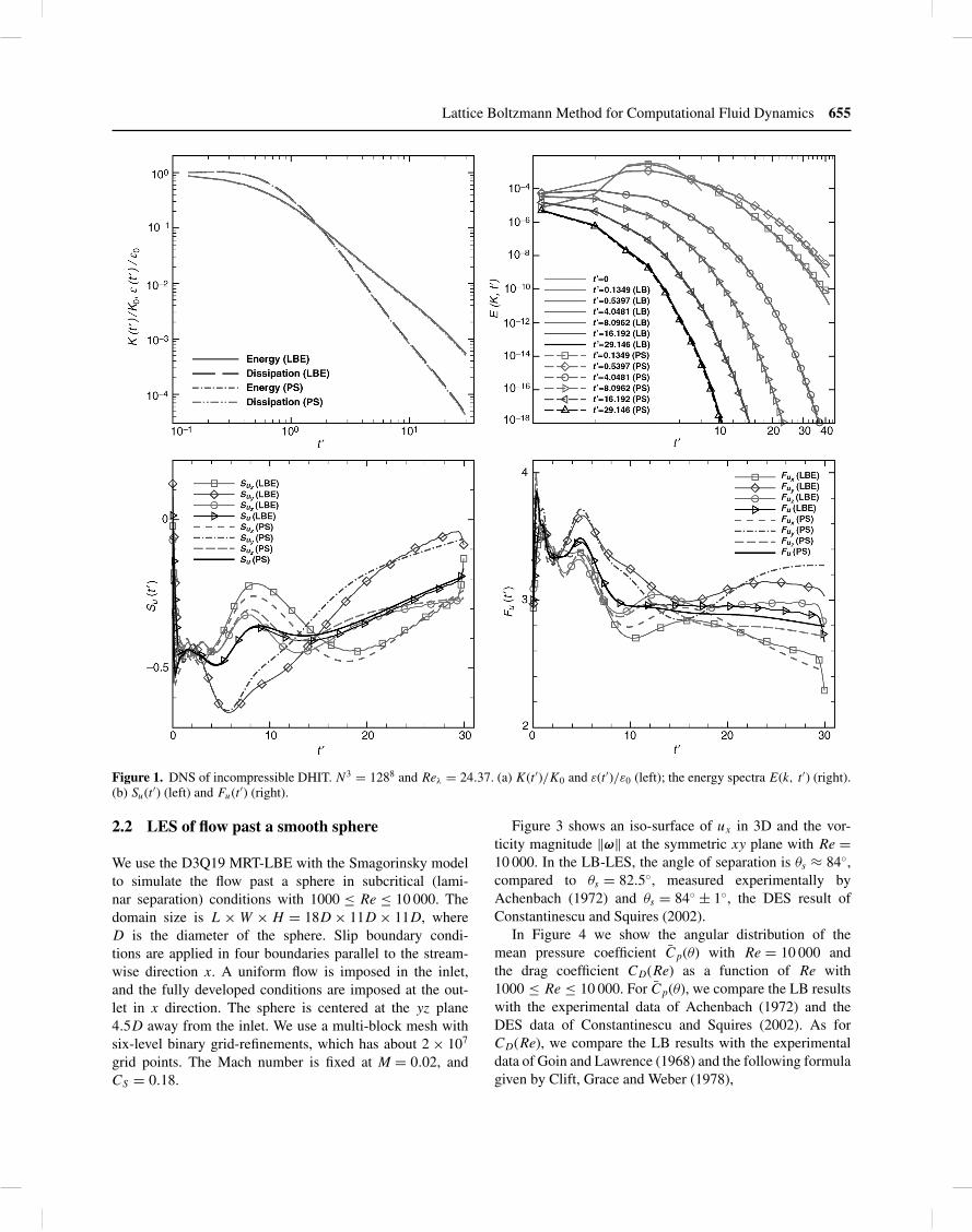
Due to the simplicity of the boundary conditions in DHIT,pseudo-spectral (PS) methods are the de facto method forthis problem. We use the D3Q19 LBE model and com-pare a pseudo-spectral (PS) method with a second-orderAdam-Bashforth scheme for time integration (Peng et al.,2009). The mesh size is N3 = 1283 and Reλ = 24.37. Thesimulations are carried out to t′ = t/τ0 ≈ 30, where τ0 =K0/ε0 is the turbulence turnover time. Both the LBE andPS methods use the same dimensionless time step size δt′ =δt/τ0.

The normalized kinetic energy K(t′)/K(0), the normalizeddissipation rate ε(t′)/ε(0), the energy spectra E(k, t′), theskewness Su(t′), and the flatness Fu(t′) are shown in Figure 1.We observe that all these statistical quantities obtained bythe LB method agree very well with those obtained by thepseudo-spectral method (Peng et al., 2009).

Figure 2 shows the instantaneous velocity and vorticityfields obtained by the LBE and the pseudo-spectral method.It is remarkable that the flow fields obtained by using thesetwo vastly different methods agree so well with each other(Peng et al., 2009).

Lattice Boltzmann Method for Computational Fluid Dynamics 655

Figure 1. DNS of incompressible DHIT. N3 = 1288 and Reλ = 24.37. (a) K(t′)/K0 and ε(t′)/ε0 (left); the energy spectra E(k, t′) (right).(b) Su(t′) (left) and Fu(t′) (right).

2.2 LES of flow past a smooth sphere

We use the D3Q19 MRT-LBE with the Smagorinsky modelto simulate the flow past a sphere in subcritical (lami-nar separation) conditions with 1000 ≤ Re ≤ 10 000. Thedomain size is L × W × H = 18D × 11D × 11D, whereD is the diameter of the sphere. Slip boundary condi-tions are applied in four boundaries parallel to the stream-wise direction x. A uniform flow is imposed in the inlet,and the fully developed conditions are imposed at the out-let in x direction. The sphere is centered at the yz plane4.5D away from the inlet. We use a multi-block mesh withsix-level binary grid-refinements, which has about 2 × 107

grid points. The Mach number is fixed at M = 0.02, andCS = 0.18.

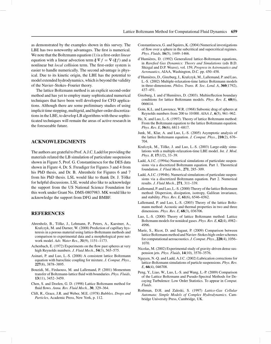
Figure 3 shows an iso-surface of ux in 3D and the vor-ticity magnitude ‖ω‖ at the symmetric xy plane with Re =10 000. In the LB-LES, the angle of separation is θs ≈ 84◦,compared to θs = 82.5◦, measured experimentally byAchenbach (1972) and θs = 84◦ ± 1◦, the DES result ofConstantinescu and Squires (2002).

In Figure 4 we show the angular distribution of themean pressure coefficient Cp(θ) with Re = 10 000 andthe drag coefficient CD(Re) as a function of Re with1000 ≤ Re ≤ 10 000. For Cp(θ), we compare the LB resultswith the experimental data of Achenbach (1972) and theDES data of Constantinescu and Squires (2002). As forCD(Re), we compare the LB results with the experimentaldata of Goin and Lawrence (1968) and the following formulagiven by Clift, Grace and Weber (1978),

656 Computational Fluid Dynamics

Figure 2. DNS of DHIT. The magnitudes of the velocity ‖u(x, t′)/u′‖ (top row) and the vorticity ‖ω(x, t′)/u′‖ (bottom row) on the xy

plane z = �. The LBE (solid lines) vs. the pseudo-spectral method (dashed lines). From left to right: t′ = 4.048 169, 8.095 571, 16.18 959,and 29.94 941.

CD ≈ e−5.657681832+2.5558x−0.04036767209x2+0.01978536702x3,

x := ln Re (22)

For both Cp(θ) and CD(Re), the LBE–LES results agreewell with existing data.

2.3 Particulate suspensions

With the bounce-back boundary conditions, the net momen-tum change due a particle-boundary collision is −2wiρuw · ci

along the direction of ci. Consequently, the total force F and

torque T on a particle are

F = −∑

ci∈Bxk∈∂�

2wiρ uw · ci ci,

T =∑

ci∈Bxk∈∂�

2wiρ uw · ci ci × (xk − r),

ci := ci

‖ci‖ (23)

where B is the set of all discrete velocities at a boundarynode xk, which intersect with the boundary, ∂� is the set ofall boundary nodes around a particle of volume �, and r isthe center of the mass. With F and T available, the particle

Figure 3. LBE-LES for the flow past a sphere at Re = 10 000. (a) Instantaneous iso-surface of ux in 3D and (b) ‖ω‖ on the symmetric xy

plane. Courtesy of S. Freudiger.

Lattice Boltzmann Method for Computational Fluid Dynamics 657

0 60 120 180

−0.5

0

0.5

1 LBE-LES, Re =10 000NS-DES, Re =10 000Exp. Re =162 000

2000(b)(a)

4000 6000 8000 10 000

0.4

0.5

TheoryExp, Ma=0.2LBE-LES

Re

CD (

Re)

Cp

(θ)

θ º

Figure 4. Flow past a sphere. (a) Cp(θ) at Re = 10 000, θ = 0◦ is the stagnation point. (b) CD(Re), 1000 ≤ Re ≤ 10 000.

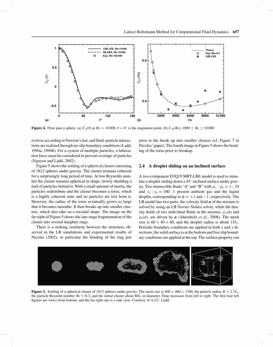
evolves according to Newton’s law, and fluid–particle interac-tions are realized through no-slip boundary conditions (Ladd,1994a, 1994b). For a system of multiple particles, a lubrica-tion force must be considered to prevent overlaps of particles(Nguyen and Ladd, 2002).

Figure 5 shows the settling of a spherical cluster consistingof 1812 spheres under gravity. The cluster remains coherentfor a surprisingly long period of time. At low Reynolds num-ber the cluster remains spherical in shape, slowly shedding atrail of particles behind it. With a small amount of inertia, theparticles redistribute and the cluster becomes a torus, whichis a highly coherent state and no particles are lost from it.However, the radius of the torus eventually grows so largethat it becomes unstable. It then breaks up into smaller clus-ters, which also take on a toroidal shape. The image on thefar right of Figure 5 shows the late-stage fragmentation of thecluster into several daughter rings.

There is a striking similarity between the structures ob-served in the LB simulations and experimental results ofNicolas (2002), in particular the bending of the ring just

prior to the break up into smaller clusters (cf. Figure 7 inNicolas’ paper). The fourth image in Figure 5 shows the bend-ing of the torus prior to breakup.

2.4 A droplet sliding on an inclined surface

A two-component D3Q19 MRT-LBE model is used to simu-late a droplet sliding down a 45◦ inclined surface under grav-ity. Two immiscible fluids “A” and “B” with ρA : ρB = 1 : 10and νA : νB = 100 : 1 present ambient gas and the liquiddroplet, corresponding to φ = +1 and −1, respectively. TheLB model has two parts: the velocity field u of the mixture issolved by using an LB Navier–Stokes solver, while the den-sity fields of two individual fluids in the mixture, ρA(x) andρB(x), are driven by u (Ahrenholz et al., 2008). The meshsize is 60 × 40 × 60, and the droplet radius is about 15δx.Periodic boundary conditions are applied in both x and y di-rections; the solid surface is at the bottom and free slip bound-ary conditions are applied at the top. The surface property can

Figure 5. Settling of a spherical cluster of 1812 spheres under gravity. The mesh size is 400 × 400 × 1300, the particle radius R ≈ 2.7δx,the particle Reynold number Re ≈ 0.3, and the initial cluster about 80δx in diameter. Time increases from left to right. The first four leftfigures are views from bottom, and the far right one is a side view. Courtesy of A.J.C. Ladd.

658 Computational Fluid Dynamics

Figure 6. Droplets sliding down a 45◦ inclined surface under gravity. (a) Left to right, φw = −0.5, 0.0, 0.5, and 1.0; (b) the final profilesof the droplet; as a reference, a symmetric droplet on a leveled surface with φw = 1.0 is also shown. Courtesy of B. Ahrenholz.

be either hydrophilic (φw < 0) or hydrophobic (φw > 0) tothe droplet. In the final state with a constant sliding velocitydepending on gravity, the droplet attains different recedingand preceding contact angles depending on the surface prop-erty specified by φw. Figure 6 shows the final states of dropletson the surfaces with different wettability. The numerical re-sults of the contact angles agree well with theoretical predic-tions.

2.5 Flow through porous media

Figure 7 shows simulations of the residual air saturation af-ter a liquid imbibition in natural soil samples (Tolke et al.,2002; Tolke, Freudiger and Krafczyk, 2006; Ahrenholz et al.,2008). A mesh of size 2003 is used to resolve the samples,which are digitized by CT scan techniques. The grid size is

δx ≈ 11 �m. The simulations can be used to determine thesensitivity of the computed transport coefficients for unsat-urated soil on porosity φ and the representative elementaryvolume necessary to derive the macroscopic transport prop-erties.

3 CONCLUSIONS AND OUTLOOK

In this article we provide a concise survey of the latticeBoltzmann equation: its mathematical theory and its capabil-ities for CFD applications. Due to the space limitation, we donot discuss the LB applications for thermo-hydrodynamics,non-Newtonian fluids, and micro-flows with non-zeroKnudsen number effects. A more extensive review has beengiven by Yu et al. (2003). Although the LBE is still in itsinfancy, it has shown great potential in a number of areas,

Figure 7. Immiscible fluids through porous media. Residual air saturation after liquid imbibition. Only the residual air is shown. (a) Theporosity φ = 0.412; (b) 0.388. Courtesy of B. Ahrenholz.

Lattice Boltzmann Method for Computational Fluid Dynamics 659

as demonstrated by the examples shown in this survey. TheLBE has two noteworthy advantages. The first is numerical.We note that the Boltzmann equation (1) is a first-order linearequation with a linear advection term ξ ·∇f = ∇·(ξf ) and anonlinear but local collision term. The first-order system iseasier to handle numerically. The second advantage is phys-ical. Due to its kinetic origin, the LBE has the potential tomodel extended hydrodynamics, which is beyond the validityof the Navier–Stokes–Fourier theory.

The lattice Boltzmann method is an explicit second-ordermethod and has yet to employ many sophisticated numericaltechniques that have been well developed for CFD applica-tions. Although there are some preliminary studies of usingimplicit time stepping, multigrid, and higher-order discretiza-tions in the LBE, to develop LB algorithms with these sophis-ticated techniques will remain the areas of active research inthe foreseeable future.

ACKNOWLEDGMENTS

The authors are grateful to Prof. A.J.C. Ladd for providing thematerials related the LB simulation of particulate suspensionshown in Figure 5, Prof. G. Constantinescu for the DES datashown in Figure 4, Dr. S. Freudiger for Figures 3 and 4 fromhis PhD thesis, and Dr. B. Ahrenholz for Figures 6 and 7from his PhD thesis. LSL would like to thank Dr. J. Tolkefor helpful discussions. LSL would also like to acknowledgethe support from the US National Science Foundation forthis work under Grant No. DMS-0807983. MK would like toacknowledge the support from DFG and BMBF.

REFERENCES

Ahrenholz, B., Tolke, J., Lehmann, P., Peters, A., Kaestner, A.,Krafczyk, M. and Durner, W. (2008) Prediction of capillary hys-teresis in a porous material using lattice-Boltzmann methods andcomparison to experimental data and a morphological pore net-work model. Adv. Water Res., 31(9), 1151–1173.

Achenbach, E. (1972) Experiments on the flow past spheres at veryhigh Reynolds numbers. J. Fluid Mech., 54(3), 565–575.

Asinari, P. and Luo, L.-S. (2008) A consistent lattice Boltzmannequation with baroclinic coupling for mixture. J. Comput. Phys.,227(8), 3878–3895.

Bouzidi, M., Firdaouss, M. and Lallemand, P. (2001) Momentumtransfer of Boltzmann-lattice fluid with boundaries. Phys. Fluids,13(11), 3452–3459.

Chen, S. and Doolen, G. D. (1998) Lattice Boltzmann method forfluid flows. Annu. Rev. Fluid Mech., 30, 329–364.

Clift, R., Grace, J.R. and Weber, M.E. (1978) Bubbles, Drops andParticles, Academic Press, New York, p. 112.

Constantinescu, G. and Squires, K. (2004) Numerical investigationsof flow over a sphere in the subcritical and supercritical regimes.Phys. Fluids, 16(5), 1449–1466.

d’Humieres, D. (1992) Generalized lattice-Boltzmann equations,in Rarefied Gas Dynamics: Theory and Simulations (eds B.D.Shizgal and D.P. Weave), vol. 159, Progress in Astronautics andAeronautics, AIAA, Washington, D.C. pp. 450–458.

d’Humieres, D., Ginzburg, I., Krafczyk, M., Lallemand, P. and Luo,L.-S. (2002) Multiple-relaxation-time lattice Boltzmann modelsin three-dimensions. Philos. Trans. R. Soc. Lond. A, 360(1792),437–451.

Ginzburg, I. and d’Humieres, D. (2003). Multireflection boundaryconditions for lattice Boltzmann models. Phys. Rev. E, 68(6),066614.

Goin, K.L. and Lawrence, W.R. (1968) Subsonic drag of spheres atReynolds numbers from 200 to 10 000. AIAA J., 6(5), 961–962.

He, X. and Luo, L.-S. (1997). Theory of lattice Boltzmann method:From the Boltzmann equation to the lattice Boltzmann equation.Phys. Rev. E, 56(6), 6811–6817.

Junk, M., Klar, A. and Luo, L.-S. (2005) Asymptotic analysis ofthe lattice Boltzmann equation. J. Comput. Phys., 210(2), 676–704.

Krafczyk, M., Tolke, J. and Luo, L.-S. (2003) Large-eddy simu-lations with a multiple-relaxation-time LBE model. Int. J. Mod.Phys. B, 17(1/2), 33–39.

Ladd, A.J.C. (1994a) Numerical simulations of particulate suspen-sions via a discretized Boltzmann equation. Part 1. Theoreticalfoundation. J. Fluid Mech., 271, 285–309.

Ladd, A.J.C. (1994b). Numerical simulations of particulate suspen-sions via a discretized Boltzmann equation. Part 2. Numericalresults. J. Fluid Mech., 271, 311–339.

Lallemand, P. and Luo, L.-S. (2000) Theory of the lattice Boltzmannmethod: Dispersion, dissipation, isotropy, Galilean invariance,and stability. Phys. Rev. E, 61(6), 6546–6562.

Lallemand, P. and Luo, L.-S. (2003) Theory of the lattice Boltz-mann method: Acoustic and thermal properties in two and threedimensions. Phys. Rev. E, 68(3), 036706.

Luo, L.-S. (2000) Theory of lattice Boltzmann method: LatticeBoltzmann models for nonideal gases. Phys. Rev. E, 62(4), 4982–4996.

Marıe, S., Ricot, D. and Sagaut, P. (2009) Comparison betweenlattice Boltzmann method and Navier–Stokes high-order schemesfor computational aeroacoustics. J. Comput. Phys., 228(4), 1056–1070.

Nicolas, M. (2002) Experimental study of gravity-driven dense sus-pension jets. Phys. Fluids, 14(10), 3570–3576.

Nguyen, N.-Q. and Ladd, A.J.C. (2002) Lubrication corrections forlattice-Boltzmann simulations of particle suspensions. Phys. Rev.E, 66(4), 046708.

Peng, Y., Liao, W., Luo, L.-S. and Wang, L.-P. (2009) Comparisonof the Lattice Boltzmann and Pseudo-Spectral Methods for De-caying Turbulence: Low Order Statistics. To appear in Comput.Fluids.

Rothman, D.H. and Zaleski, S. (1997) Lattice-Gas CellularAutomata: Simple Models of Complex Hydrodynamics. Cam-bridge University Press, Cambridge, UK.

660 Computational Fluid Dynamics

Tolke, J., Freudiger, S. and Krafczyk, M. (2006) An adaptive schemeusing hierarchical grids for lattice Boltzmann multi-phase flowsimulations. Comput. Fluids, 35(8/9), 820–830.

Tolke, J., Krafczyk, M., Schulz, M. and Rank, E. (2002) LatticeBoltzmann simulations of binary fluid flow through porous me-dia. Philos. Trans. R. Soc. Lond. A, 360(1792), 535–545.

Yu, D., Mei, R., Luo, L.-S. and Shyy, W. (2003) Viscous flow com-putations with the method of lattice Boltzmann equation. Prog.Aerospace Sci., 39(5), 329–367.

Yu, H., Luo, L.-S. and Girimaji, S.S. (2006) LES of turbulent squarejet flow using an MRT lattice Boltzmann model. Comput. Fluids,35(8/9), 957–965.