
Lattice Boltzmann Methods for Single and Two ... - POLITesi
200
POLITECNICO DI MILANO Scuola di Ingegneria Industriale e dell’Informazione Corso di Laurea Specialistica in Ingegneria Energetica Lattice Boltzmann Methods for Single and Two-Phase Flows in Porous Media: Theory and Applications Relatore: Prof. Fabio Inzoli Co-relatori: Ing. Ga¨ el Gu´ edon Prof. Pietro Asinari Tesi di Laurea di: Alessandro Ciani Matr. 783130 Anno Accademico 2012-2013
-
Upload
khangminh22 -
Category
Documents
-
view
4 -
download
0
Transcript of Lattice Boltzmann Methods for Single and Two ... - POLITesi

POLITECNICO DI MILANO
Scuola di Ingegneria Industriale e dell’Informazione
Corso di Laurea Specialistica in Ingegneria Energetica
Lattice Boltzmann Methods for Single and Two-PhaseFlows in Porous Media: Theory and Applications
Relatore: Prof. Fabio InzoliCo-relatori: Ing. Gael Guedon
Prof. Pietro Asinari
Tesi di Laurea di:Alessandro Ciani Matr. 783130
Anno Accademico 2012-2013

A mamma e papa
II

Ringraziamenti
Vorrei iniziare con il ringraziare il Prof. Fabio Inzoli ed il suo gruppo peravermi dato la possibilita di affrontare questo bellissimo argomento e peravermi guidato in questi mesi. Particolari ringraziamenti vanno sicuramenteall’Ing. Gael Guedon che mi ha dedicato molto del suo tempo, e con cui hopotuto condividere dubbi e problemi, specialmente nella parte computazio-nale della tesi, in cui ha dimostrato le sue doti da programmatore. Ringrazioanche l’Ing. Leila Moghadasi per avermi introdotto alla materia di questatesi, e per avermi fornito sostegno durante il percorso. Ci tengo, inoltre,a ringraziare il Prof. Pietro Asinari per la gentilezza che ha mostrato nelnostro incontro e per i suoi saggi consigli.
Un enorme grazie va a tutti coloro che mi hanno supportato durantequesto periodo della mia vita e che hanno contribuito in qualche modo alraggiungimento di questo traguardo.
Fra queste innumerevoli persone, il primo ringraziamento va a mia madreDina, che e stata il mio punto di riferimento costante in tutti questi anni diuniversita e che, fin da quando ero bambino, ha fatto degli enormi sacrificiper rendere suo figlio felice e consentirgli di raggiungere i suoi obiettivi.
Ringrazio la mia ragazza Cecilia, che mi e stata sempre vicina durantequesti mesi e che con il suo amore e riuscita a rendere felici le mie giornate,anche quando ci sono state delle difficolta.
Particolari ringraziamenti vanno alle due nonne Natalina e Germana, chevogliono un bene dell’anima al loro nipote. Vorrei ringraziare mio zio Adria-no, mia zia Daniela ed i miei cugini Alessandra e Francesco semplicementeper avermi fatto sentire a casa ogni volta che sono tornato. Un grazie va an-che a mio zio Nevio e mia zia Lucia, che mi hanno aiutato in questa trasfertamilanese.
Inoltre, ringrazio tutti i miei amici con i quali condivido la mia vita. Inparticolare, ci tengo a ringraziare le mie coinquiline Federica, Mariagrazia eCristina, con le quali ho percorso giorno dopo giorno questo cammino e cheormai sono come una seconda famiglia per me.
Infine, ringrazio mio padre Dino e mio nonno Alessandro, che rappresen-tano per me degli esempi di vita, ma che purtroppo non possono condividere
III

Ringraziamenti
con me questo momento. Sono sicuro che sareste orgogliosi di me.
IV

Sommario Esteso
Lo scopo principale di questa tesi e quello di esplorare le capacita dei metodiLattice Boltzmann (LBM) nelle simulazioni di flussi monofase e bifase, conparticolare focus sulle applicazioni ai mezzi porosi.
Sorti a cavallo tra gli anni ottanta e novanta, dalle ceneri del cosiddettoLattice Gas Automaton (LGA), i metodi Lattice Boltzmann si propongonocome metodi alternativi alla fluidodinamica computazionale convenzionale,basata sulla discretizzazione ed integrazione diretta delle equazioni di Navier-Stokes. Gli LBM, infatti, forniscono una descrizione su una scala inferiorerispetto a quella macroscopica, da cui pero, come vedremo, emergono le equa-zioni che governano il mondo macroscopico. Tale scala viene comunementedetta mesoscopica, poiche intermedia fra la scala microscopica, propria adesempio della Molecular Dynamics, e appunto macroscopica, cioe di validitadell’ipotesi del continuo su cui si basano le equazioni di Navier-Stokes.
I metodi Lattice Boltzmann fondano le loro radici nella meccanica stati-stica, di cui Ludwig Boltzmann ne e il padre e per questo compare nel nomestesso dei metodi. In particolare, vedremo che e stato dimostrato il legamediretto fra l’equazione di Boltzmann e la cosiddetta “Lattice Boltzmann equa-tion” (LBE), seppur cio e avvenuto storicamente dopo l’introduzione degliLBM. Il termine “Lattice” invece si riferisce alla tipica struttura della grigliadi discretizzazione degli LBM, che e caratterizzata da un alto grado di sim-metria. Un esempio e riportato in Fig. 1, per un caso di lattice a simmetriaesagonale. Tale struttura deriva sostanzialmente da un elemento caratteri-stico degli LBM, cioe la discretizzazione dello spazio delle velocita. Infatti,l’oggetto della LBE sono, appunto, le funzioni di probabilita associate a talivelocita discrete.
Uno dei vantaggi fondamentali degli LBM e la semplicita dell’algoritmo,in un certo senso indotta dall’alta simmetria della griglia. In aggiunta, l’algo-ritmo ha un carattere puramente locale, il che permette una diretta paralleliz-zazione. A queste caratteristiche, si aggiungono altri vantaggi, che risultanoessere particolarmente adatti al contesto dei mezzi porosi. In primis, c’e lafacile gestione di geometrie complesse. Cio e dovuto alla possibilita di mo-dellare l’interazione con le pareti solide attraverso delle semplici condizioni
V

Sommario Esteso
Figura 1. Esempio di lattice a simmetria esagonale.
al contorno, dette di Bounce-Back, che cercano appunto di riprodurre l’urtodelle particelle con le pareti. Di fatto, la geometria di input e costituita dauna semplice griglia booleana, in cui si identificano nodi di fluido e di solido.Data tale semplicita, tutte le geometrie utilizzate in questa tesi sono stategenerate dall’autore con semplici scripts scritti in ambiente Matlab. In se-conda istanza, gli LBM consentono di simulare sistemi multifase con relativasemplicita. Il vantaggio principale e che non e necessaria una modellazio-ne dell’interfaccia, ma la sua dinamica viene riprodotta in maniera naturaledalle forze di interazioni fra le particelle, che possono essere introdotte nelmetodo. Come possiamo intuire, sia la facile gestione di geometrie complesse,sia i vantaggi nel simulare flussi multifase, derivano dalla natura mesoscopicadegli LBM. Inoltre, nelle applicazioni ai mezzi porosi, diversi problemi degliLBM tendono a risolversi, date le peculiari condizioni del flusso. In definiti-va, il contesto dei mezzi porosi e uno dei campi naturali di applicazione degliLBM.
In questa tesi, dunque, viene portata a termine un’analisi dei metodiLattice Boltzmann, sia a livello teorico, che applicativo, per flussi monofasee bifase. Dopo una iniziale introduzione ai concetti fondamentali dei flussinei mezzi porosi, che verranno utilizzati nella parte di simulazioni, i metodiLattice Boltzmann vengono descritti riportando la loro derivazione dall’equa-zione di Boltzmann. Tale approccio viene preferito rispetto alla derivazionestorica, in quanto fornisce una visione piu moderna degli LBM, ed anchepiu rigorosa. Questa parte e stata inserita, poiche ritenuta necessaria perla comprensione delle tematiche sviluppate in questa tesi. In particolare,l’equazione di Boltzmann viene descritta nel dettaglio, cosı come il collega-mento con le grandezze macroscopiche. Partendo da tali fondamenta, vieneriportata la procedura di discretizzazione dell’equazione di Boltzmann, cheporta alla Lattice Boltzmann equation, sottolineando i passaggi critici di taledimostrazione. I concetti sviluppati per l’equazione di Boltzmann vengonopoi traslati naturalmente nel mondo discreto degli LBM.
A valle di questa derivazione, viene mostrato il collegamento con le equa-
VI

Sommario Esteso
zioni di Navier-Stokes, mediante la cosiddetta espansione di Chapman-Enskog.Tale espansione e fondamentalmente un metodo perturbativo multi-scala,utilizzato anche per mostrare la connessione dell’equazione di Boltzmanncon le equazioni macroscopiche. La procedura riportata e stata ripresa dallavoro di Kuzmin [1], ma viene fornita una dimostrazione piu generale chemostra il metodo piu opportuno per l’introduzione delle forze, siano esseesterne o interagenti, nella Lattice Boltzmann equation.
Per completare l’apparato teorico degli LBM viene anche affrontato iltema delle condizioni al contorno. Innanzitutto, viene spiegato il significa-to delle condizioni al contorno in tale modellazione mesoscopica. Possiamoinfatti intuire come le condizioni al contorno debbano riguardare le variabilidella Lattice Boltzmann equation, cioe le funzioni di distribuzione associatealle velocita discrete. Cio porta a distinguere fra due approcci. Il primoin cui si sfrutta l’interpretazione mesoscopica dei metodi; nel secondo, inve-ce, si cerca di traslare condizioni al contorno sulle velocita o sulla pressionein termini delle funzioni di distribuzione discrete. In questa parte, solo lecondizioni al contorno che verranno utilizzate nella tesi sono analizzate.
L’analisi applicativa viene svolta interamente nel caso bidimensionale.Tale scelta ha svariate motivazioni. Innanzitutto, il caso 2D permette unapiu semplice e veloce individuazione delle caratteristiche salienti dei metodi.In seconda istanza, data la simmetria inerente ai metodi, il passaggio allaterza dimensione e diretto e non aggiunge di fatto nulla alla trattazione. Ciogiustifica anche il fatto che la letteratura degli LBM si focalizza soprattuttosu problemi bidimensionali.
Lo strumento utilizzato per le simulazioni e la libreria open-source Palabos,sviluppata recentemente da una collaborazione fra “The FlowKit Ltd. tech-nology company” e l’Universita di Ginevra. La libreria Palabos e scrittaintegralmente in C++, che e dunque stato l’ambiente di sviluppo di tutti icodici Lattice Boltzmann utilizzati in questa tesi.
La parte applicativa monofase ha riguardato tre casi studio:
1. il flusso di Hagen-Poiseuille in un canale bidimensionale;
2. il flusso in una schiera di dischi disposti esagonalmente;
3. il flusso in una schiera di dischi con disposizione casuale.
Il primo semplice caso di flusso laminare in un canale bidimensionale e sta-to utilizzato per avere una prima validazione degli LBM e per evidenziarealcune caratteristiche fondamentali, che poi si ripercuotono in qualunqueapplicazione piu complessa. Infatti, tale flusso e sicuramente il piu studia-to nella letteratura degli LBM. E inoltre intuitiva l’analogia fra il flusso diHagen-Poiseuille ed il flusso in un canale di un mezzo poroso. I risultati
VII

Sommario Esteso
sono confrontati con la soluzione analitica, nota per questo problema, masono anche utilizzati per verificare i risultati teorici sugli LBM descritti nellaparte iniziale della tesi, mostrando, in entrambi i casi, un generale accordo.
La seconda geometria e stata invece scelta perche rappresenta un primocaso di mezzo poroso, in cui sono disponibili soluzioni semi-analitiche perla permeabilita del mezzo, che permettono, anche qui, un confronto con irisultati numerici. Inoltre, la periodicita del sistema in questione, che vieneassunto infinito, consente di studiare il flusso nella sola cella elementare. Co-me soluzioni di riferimento sono state utilizzate le correlazioni di Drummond& Tahir [2], e quella piu recente di Tamayol & Bahrami [3]. La seconda equella che ha mostrato il migliore accordo con i risultati numerici degli LBM.
Infine, come conclusione della parte monofase, l’attenzione e volta ad unageometria piu rappresentativa di un mezzo poroso reale, costituita da unaschiera di dischi disposti casualmente. L’obiettivo di tale studio e quello diverificare la validita del modello di Carman-Kozeny per predire la permea-bilita. Svariate geometrie random sono state generate per effettuare taleverifica, in modo da consentire una statistica dei risultati. Le simulazionihanno confermato che il modello di Carman-Kozeny e un modello valido pertale geometria, specialmente quando la porosita del mezzo e moderata. Nel-la trattazione vengono anche analizzate in maniera qualitativa le cause degliscostamenti dal modello mostrati da alcune geometrie.
Alla parte applicativa monofase, segue la parte teorica di introduzione aimodelli Lattice Boltzmann (LB) per flussi multifase. Il modello utilizzato inquesta tesi e quello proposto da Shan & Chen (SC) [4], che e storicamenteil primo modello LB proposto per flussi multifase, ed anche il piu semplicefra quelli presenti in letteratura. Inoltre, il modello di Shan & Chen risultafacilmente implementabile nell’ambiente Palabos. In questa tesi il modello diShan & Chen verra utilizzato solo nel caso bifase, seppure e possibile simulareanche piu fasi.
L’idea principale dietro il modello di Shan & Chen risiede nell’introduzio-ne di una forza di interazione fra un nodo del lattice e i suoi “primi vicini”,capace di innescare una separazione di fase in determinate condizioni. A suavolta, possono essere distinti svariati sottomodelli dello Shan-Chen a secon-da della forma assunta da tale interazione. Possiamo quindi intuire, come lamodellazione multifase ottenuta con il metodo di Shan & Chen debba sotto-stare alle leggi che governano la separazione di fase del modello. Ad esempio,il rapporto di densita fra i due fluidi non e un parametro di input, ma vaottenuto calibrando i parametri del modello.
Caratteristica principale del modello di Shan & Chen per flussi multifa-se e la presenza di una interfaccia finita e diffusa, e quindi non infinitesi-ma. Questa peculiarita e condivisa anche da altri modelli multifase Lattice
VIII

Sommario Esteso
Boltzmann.Una volta ottenuta l’equazione di stato, che consente di individuare i pa-
rametri critici del modello, la natura immiscibile del sistema viene studiatamediante applicazioni statiche, da cui si possono ottenere dei diagrammi distato. In questa parte ci si riferisce sempre alla formulazione originale delmodello di Shan & Chen. Viene anche mostrato come da semplici test siapossibile ottenere grandezze come la tensione superficiale o l’angolo di con-tatto. Il comportamento nelle vicinanze del punto critico del modello vieneanalizzato, mostrando analogie con altri fenomeni critici. Particolare enfasi eposta sui problemi di questo modello, che ne limitano le applicazioni a flussicon moderati rapporti di densita fra le due fasi. Cio e dovuto alle cosiddettecorrenti spurie, delle velocita artificiali prodotte dal modello nelle vicinan-ze all’interfaccia. Tali correnti sono in qualche modo legate al rapporto didensita, ed essendo molto elevate, causano instabilita del modello quandotale rapporto aumenta. In aggiunta, si pone, in generale, un problema diambiguita nella distinzione fra tali velocita artificiali e le velocita fisiche, chesi manifesta anche a bassi rapporti di densita.
La letteratura sul modello di Shan & Chen si e focalizzata negli ultimianni sulla risoluzione di questi problemi. In particolare, in questa tesi vienesvolta un’analisi del metodo proposto da Yuan & Schaefer [5], che consistesostanzialmente nel cambiare la forma dell’interazione, in modo da soddisfa-re equazione di stato fisiche, di cui la Peng-Robinson e la Carnahan-Starlingne sono esempi. Tale metodo viene descritto nel dettaglio ed implementatonell’ambiente Palabos. Cio ha richiesto una espansione della libreria origi-nale di Palabos, poiche nell’attuale versione l’incorporazione delle equazionidi stato nel modello di Shan & Chen non e direttamente disponibile. Vienequindi mostrato mediante dei test, come, fissato un rapporto di densita, siapossibile ottenere una riduzione delle correnti spurie, e come da cio derivi unaumento del rapporto di densita limite simulabile, anche di ordini di grandez-za. Tuttavia, viene puntualizzato il problema di trovare una inizializzazionestabile delle densita, che si traduce, di fatto, in una procedura di “trial anderror”.
Il modello viene sottoposto ad una prima validazione dinamica nel casodi flusso laminare bifase, simile al caso di flusso di Hagen-Poiseuille, per cuia sua volta e disponibile una soluzione analitica. Tale flusso e quello ge-neralmente usato per validare il modello in letteratura e fornisce un primoesempio di flusso in un mezzo poroso. Il problema viene studiato per i tremodelli di interazione del modello di Shan & Chen esaminati, cioe la formu-lazione originale, e le due versioni con la equazioni di stato di Carnahan &Starling e di Peng & Robinson. E stato scelto per il confronto un rapporto didensita moderato, in modo da ottenere una configurazione stabile per tutti
IX

Sommario Esteso
i modelli. In questo caso, si evidenzia come per tale rapporto di densita ilmodello originale, mostri un migliore accordo con la soluzione analitica, acausa del minore spessore dell’interfaccia presentata da tale modello. Tutta-via, viene anche mostrato un primo effetto delle correnti spurie che affliggemaggiormente il modello originale.
In conclusione, i metodi Lattice Boltzmann sono stati discussi sia a livelloteorico che pratico, mediante diversi casi studio. Gli LBM si sono dimostra-ti senza dubbio uno strumento valido per lo studio dei flussi monofase neimezzi porosi. Lo studio di flussi bifase mediante gli LBM e stato introdottoutilizzando il modello di Shan & Chen. Le caratteristiche, le potenzialita e leproblematiche di tale modello sono state discusse ampiamente, analizzandoi risultati delle simulazioni. Oltre al modello originale, sono stati studiatidei suoi miglioramenti implementandoli in ambiente Palabos. Sottoponendoi modelli a diversi test statici e ad una prima validazione dinamica, si e mo-strato che molti problemi della formulazione originale possono essere ridotti,seppur il modello originale puo essere preferibile in alcuni casi.
Le prospettive future di questa tesi sono svariate. In prima istanza,l’applicazione dei metodi Lattice Boltzmann puo essere estesa a casi studiodi mezzi porosi reali tridimensionali. Inoltre, i risultati teorici ottenuti perl’introduzione delle forze nella Lattice Boltzmann equation, possono essereconfermati con dei test numerici. Per quanto riguarda la parte bifase, il mo-dello di Shan & Chen puo essere ulteriormente migliorato introducendo altrecorrezioni proposte in letteratura. In aggiunta, il modello puo essere validatoin un caso piu complesso rispetto a quello considerato, in cui i problemi adesso connessi potrebbero avere una maggiore influenza.
X

Extended Abstract
The main purpose of this thesis is to explore the capabilities of the Lat-tice Boltzmann methods (LBMs) for the simulation of single- and two-phaseflows, with particular focus on porous media applications.
Historically, the Lattice Boltzmann methods arose between the eight-ies and the nineties from the ashes of the so-called Lattice Gas Automaton(LGA). They represent an alternative approach to the standard computa-tional fluid dynamics, which is based on the direct discretization and inte-gration of the Navier-Stokes equations. In fact, the LBMs provide a descrip-tion at a lower scale compared to the macroscopic scale of the Navier-Stokesequations. However, we will see that from this description, the equations thatgovern the macroscopic world arise naturally. The characteristic scale of theLBMs is usually called the mesoscopic scale, because it is halfway betweenthe microscopic scale, typical of Molecular Dynamics, and the macroscopicscale, that is the scale of validity of the continuum hypothesis, which allowsto obtain the Navier-Stokes equations.
The Lattice Boltzmann methods have roots in Statistical Mechanics,whose father is certainly Ludwig Boltzmann, and for this reason, his nameappears in the name of the methods. In particular, it has been proved thedirect relationship between the Boltzmann equation and the Lattice Boltz-mann equation (LBE), even though this has been achieved several years laterthe introduction of the LBMs. The word “Lattice” refers to the typical dis-cretization grid of the LBMs, which is characterized by a high degree ofsymmetry. An example is reported in Fig.2 for the case of an hexagonal lat-tice. This structure is basically a consequence of a characteristic feature ofLBMs, that is the discretization of the velocity space. In fact, the variablesof the LBE are the probability density functions associated to these discretevelocities.
One of the main advantages of the LBMs is the simplicity of the algo-rithm, which is somehow induced by the high symmetry of the grid. Inaddition, the algorithm is purely local, which allows a direct parallelization.In the context of porous media, also other features of the LBMs seem par-ticularly suited. In the first instance, there is the easy handling of complex
XI

Extended Abstract
Figure 2. Example of lattice with hexagonal symmetry.
geometries. This is essentially due to the possibility of modelling the inter-action of the particles with walls by means of simple boundary conditions,usually called Bounce-Back boundary conditions, which try to reproduce thecollision between particles and the solid walls. As a consequence, the inputgeometry of the LBMs is simply a boolean grid, in which we identify fluidnodes and solid nodes. Because of this simplicity, all the geometries used inthis thesis have been generated by the author with simple scripts written inthe Matlab environment. In the second instance, the LBMs allow to simulatemulti-phase flows with relative simplicity. In this case, the main advantageis that we do not need to model the behaviour of the interface, but its dy-namics arises naturally from the interactions between particles, which canbe introduced in the methods. We can say that both the easy handling ofcomplex geometries and the advantages in simulating multiphase flows aredue to the mesoscopic nature of the LBMs. Ultimately, the context of porousmedia is one of the natural fields of application of the LBMs.
In this thesis, a theoretical and practical analysis of the Lattice Boltz-mann methods is carried out for single- and two-phase flows. After an initialintroduction to the basic concepts of flows in porous media, which will beused in the simulation part, the Lattice Boltzmann method are described,reporting their derivation from the Boltzmann equation. This approach hasbeen preferred over the historical derivation from the Lattice Gas model, be-cause it represents the modern interpretation of the LBMs, and it is also themost rigorous procedure. This part has been included, since it was consid-ered necessary for the understanding of the themes discussed in this thesis.In particular, the Boltzmann equation is described in details, as well as theconnections to the macroscopic quantities. Starting from these solid basis,the discretization of the Boltzmann equation is reported, highlighting thecritical passages of this proof, and finally the Lattice Boltzmann equationis obtained. In this way, the main concept introduced for the Boltzmannequation are naturally translated in the discrete world of the LBM.
After this derivation, the connection to the Navier-Stokes equations is
XII

Extended Abstract
shown by means of the so-called Chapman-Enskog expansion. This expan-sion is basically a multi-scale perturbative method, that has been used alsoto show the connection between the Boltzmann equation and the macro-scopic equations. The procedure here reported is similar to that describedby Kuzmin [1], but it is carried out in a more general case, in order to showthe most appropriate way of including the forcing term in the Lattice Boltz-mann equation.
In order to complete the theoretical framework of the LBMs, also theissue of boundary conditions is analysed. First of all, an explanation ofthe meaning of boundary conditions in the LBMs is provided. In fact, it isintuitive that the boundary conditions should concern the variables of theLBE, i.e., the distribution functions associated to the discrete velocities. Wecan distinguish between two approaches to boundary conditions in LBMs.In the former, the mesoscopic nature of the methods is exploited; instead, inthe latter, the macroscopic boundary conditions on velocity or pressure areexpressed in terms of the distribution functions. In this part of this thesis,only the boundary conditions that will be used in the simulation part areanalysed.
The application analysis is carried out entirely in two dimensions. Thereason of this choice are several. First of all, the 2D case allows a quicker andeasier identification of the main characteristics of the methods. Moreover,given the inherent symmetry of the lattice, the passage from two to threedimensions is straightforward and it does not add new elements. These arealso the reasons why the most part of the literature about LBM is developedfor the two-dimensional case.
The tool used for the simulations is Palabos, an open-source library, re-cently developed by a collaboration between the “The Flow Kit Ltd. technol-ogy company” and the University of Geneva. The Palabos library is writtenin C++, which has been the development environment of all the LatticeBoltzmann codes used in this thesis.
The single-phase part has focused on three case studies:
1. the Hagen-Poiseuille flow in a two-dimensional channel;
2. the flow over an hexagonal array of disks;
3. the flow over a random array of disks.
The first simple case of laminar flow in a two-dimensional channel has beenused to obtain a first validation of the LBMs and to highlight some basicfeatures, which characterize also any other application. In fact, this kind offlow is certainly the most studied one in the LBMs’ literature. In addition,the analogy between the Hagen-Poiseuille flow and the flow in the channel
XIII

Extended Abstract
in a porous medium is evident. The results have been compared with theanalytical solution, which is known for this case, but they have been alsoused to verify some theoretical findings about the LBMs. In both cases, thenumerical results have shown a general agreement with the theory.
The second geometry has been chosen because it represents a first andmore complex case of porous medium, in which semi-analytical formulas areavailable for the permeability, allowing even in this case a comparison withthe numerical results. As reference solutions, the correlations proposed byDrummond & Thair [2] and by Tamayol & Bahrami [3] have been selected. Inparticular, the second one has shown the best agreement with the numericalresults.
As a conclusion of the single-phase part, the attention is turned to ageometry, that is more representative of a porous medium, composed of arandom array of disks. The objective of this study is to verify the validityof the Carman-Kozeny (CK) model for the prediction of the permeability.Several random geometries have been generated, in order to obtain a statisticsof the results. The simulations have confirmed the validity of the CK modelfor this geometry, especially at moderate porosities. In the dissertation alsothe reasons of the discrepancies shown by some geometries is qualitativelyanalysed.
After the single-phase part, the theory of the Lattice Boltzmann methodsfor multi-phase flows is introduced. The model used in this thesis is theShan-Chen model proposed in [4], which is the first LBM model for multi-phase flows, and also the simplest one among those available in literature.Moreover, the Shan-Chen model can be readily implemented in the currentversion of the Palabos library. In this thesis, the Shan-Chen model has beenused to simulate only two-phase flows, even though the simulation of morephases is possible.
The basic idea behind the Shan-Chen model lies in the introduction of aninteraction force between a node of the lattice and its “nearest neighbours”,which is able to trigger phase separation in certain conditions. In turn,different sub-models of the Shan-Chen model can be distinguished dependingon the form of this interaction. It is easy to realize, that the multi-phasemodelling with the Shan-Chen model must obey the laws that govern thephase separation of the model. For instance, this means that the densityratio is not an input parameter, but has to be obtained from a preliminarycalibration phase of the model.
One of the main characteristics of the Shan-Chen model for multi-phaseflows is the presence of a finite and diffusive interface, and thus, not infinites-imal. This peculiarity of the Shan-Chen model is shared also by other LatticeBoltzmann models for multi-phase flows.
XIV

Extended Abstract
After obtaining the equation of state of the model, which allows to iden-tify the critical parameter of the phase transition, the immiscible nature ofthe model is investigated by means of static tests, from which it is possibleto obtain the phase diagrams. In this part, we refer to the original formu-lation of the Shan-Chen model. It is shown how, by means of simple tests,quantities like the surface tension and the contact angle can be calibratedand computed. The behaviour near the critical point is analysed, providinganalogies with other critical phenomena. The drawbacks of the model, whichlimit its applications to problems with limited density ratio, are emphasizedas well. This is mainly due to the so-called spurious currents, i.e., artificialvelocities produced by the model at the interface. These currents are some-how connected to the density ratio between the two phases, and cause theinstability of the model when this ratio increases. In addition, they generatealso a general problem of ambiguity between physical and artificial velocities,which manifests itself even at low density ratios.
In the last years, the literature about the Shan-Chen model has focusedon the solution of these problems. In particular, in this thesis, the methodproposed by Yuan & Scahefer [5] is analysed. This method consists in themodification of the interaction force, in order to obtain physical equation ofstate, such as the Peng-Robinson (PR) and the Carnahan-Starling (CS). Thismethod is described in details and implemented in the Palabos environment.This has required an expansion of the original library of Palabos, since inthe current version, the incorporation of physical equations of state in theShan-Chen model is not readily available. By means of simple tests, it isshown how it is possible to reduce the magnitude of the spurious velocities,given a fixed density ratio, and it is possible to simulate systems with higherdensity ratios, even by a orders of magnitude. However, it is also pointed outthe problem of finding a stable initialization of the densities, which basicallyreduce the initialization to a “trial and error” procedure.
A first dynamic validation of the model is carried out in the case of alaminar co-current flow in a 2D channel, for which an analytical solution isavailable. This flux is in general the one used in literature to validate themodel and it is a first example of flow in a channel of a porous medium.This flux is studied for the three interactions of the Shan-Chen model ex-amined in this thesis, namely the original formulation, and the two versionswith the Carnahan-Starling and Peng-Robinson equations of state. For thecomparison, a case with a limited density ratio has been chosen, in order toobtain a stable configuration for all the models. The simulations have shownthat for this limited density ratio, the original formulation of the Shan-Cheninteraction should be preferred, because it shows a better agreement with theanalytical solutions, compared to the CS and PR. This is due to the lower
XV

Extended Abstract
thickness of the interface of the original Shan-Chen model. Nevertheless, itis also shown a first effect of the spurious currents which afflicts mainly theoriginal model.
As a conclusion, the Lattice Boltzmann methods have been discussed atthe theoretical and practical level, by means of several case studies. TheLBMs have proved to be without doubts a valid tool for the study of single-phase flows in porous media. The study of two-phase flows has been intro-duced using the Shan-Chen model. The characteristics, the potentialitiesand the drawbacks of this model have been highlighted, analysing the resultsof the numerical simulations. Some improvements of the original model havebeen implemented in the Palabos library. By means of static tests and a firstdynamic validation, it has been shown how many problems of the originalformulation can be reduced, even though the original model might be moreadvisable in some cases.
The future perspectives of this thesis are several. In the first instance,the application of the Lattice Boltzmann methods may be extended to realthree-dimensional porous media. In addition, the theoretical results obtainedfor the introduction of the forcing term in the LBE might be confirmed bynumerical tests. About the two-phase part, further improvements of theShan-Chen model might be implemented in the Palabos library. Moreover,the model needs a validation in a more complex case than the 2D co-currentflow, in which the problems of the Shan-Chen model may have a greaterinfluence on the solution.
XVI

Contents
Ringraziamenti III
Sommario Esteso V
Extended Abstract XI
Sommario XXVII
Abstract XXIX
1 Introduction 11.1 Literature Review of LBM . . . . . . . . . . . . . . . . . . . . 31.2 Motivations and organization of the thesis . . . . . . . . . . . 6
2 Fluid flow in porous media 92.1 The Navier-Stokes equations . . . . . . . . . . . . . . . . . . . 102.2 The Hagen-Poiseuille flow . . . . . . . . . . . . . . . . . . . . 122.3 Stokes flow and Darcy’s law . . . . . . . . . . . . . . . . . . . 142.4 The Carman-Kozeny equation . . . . . . . . . . . . . . . . . . 16
2.4.1 Tortuosity . . . . . . . . . . . . . . . . . . . . . . . . . 172.5 Multi-phase flow . . . . . . . . . . . . . . . . . . . . . . . . . 18
2.5.1 Laplace’s law . . . . . . . . . . . . . . . . . . . . . . . 182.5.2 Wettability and capillary effects . . . . . . . . . . . . . 192.5.3 Relative Permeability . . . . . . . . . . . . . . . . . . . 21
3 The Lattice Boltzmann method 273.1 The ancestor: Lattice Gas Automaton . . . . . . . . . . . . . 283.2 The Boltzmann Equation . . . . . . . . . . . . . . . . . . . . . 313.3 Collision invariants and equilibrium distribution . . . . . . . . 333.4 From mesoscopic to macroscopic description . . . . . . . . . . 343.5 The dimensionless Boltzmann equation: the Knudsen number 383.6 The BGK approximation . . . . . . . . . . . . . . . . . . . . . 393.7 From BE to LBE . . . . . . . . . . . . . . . . . . . . . . . . . 40
XVII

Contents
3.7.1 BE as an ODE . . . . . . . . . . . . . . . . . . . . . . 413.7.2 Low Mach number expansion of the equilibrium distri-
bution . . . . . . . . . . . . . . . . . . . . . . . . . . . 413.7.3 Discretization of the velocity space . . . . . . . . . . . 42
3.8 The Multiple-Relaxation-Time model . . . . . . . . . . . . . . 49
4 The Chapman-Enskog expansion 554.1 The role of δt . . . . . . . . . . . . . . . . . . . . . . . . . . . 554.2 Inclusion of the forcing term . . . . . . . . . . . . . . . . . . . 564.3 The Chapman-Enskog multi-scale expansion . . . . . . . . . . 584.4 Restoration of macroscopic equations . . . . . . . . . . . . . . 59
4.4.1 Mass equation . . . . . . . . . . . . . . . . . . . . . . . 604.4.2 Momentum Equation . . . . . . . . . . . . . . . . . . . 61
4.5 Beyond the Chapman-Enskog expansion . . . . . . . . . . . . 67
5 Boundary conditions in LBM 695.1 Meaning of boundary conditions in LBM . . . . . . . . . . . . 705.2 Wall interaction: the Bounce-Back rule . . . . . . . . . . . . . 71
5.2.1 Geometry dependency on relaxation parameters . . . . 715.3 Periodic boundary conditions . . . . . . . . . . . . . . . . . . 745.4 Boundary conditions from moments’ perspective . . . . . . . . 755.5 Zou-He boundary conditions . . . . . . . . . . . . . . . . . . . 76
6 Porous Media applications 796.1 The tool: Palabos . . . . . . . . . . . . . . . . . . . . . . . . . 806.2 Simulation setup . . . . . . . . . . . . . . . . . . . . . . . . . 806.3 Convective and diffusive scaling . . . . . . . . . . . . . . . . . 836.4 Hagen-Poiseuille simulations . . . . . . . . . . . . . . . . . . . 846.5 Hexagonal array of disks . . . . . . . . . . . . . . . . . . . . . 936.6 Random array of disks . . . . . . . . . . . . . . . . . . . . . . 99
6.6.1 Geometry generation and simulation setup . . . . . . . 1006.6.2 How to compute tortuosity numerically . . . . . . . . . 1046.6.3 Results . . . . . . . . . . . . . . . . . . . . . . . . . . . 105
7 Lattice Boltzmann methods for multi-component and multi-phase flows: the Shan-Chen model 1137.1 Model description . . . . . . . . . . . . . . . . . . . . . . . . . 1157.2 Static tests . . . . . . . . . . . . . . . . . . . . . . . . . . . . 1207.3 Incorporating EOS . . . . . . . . . . . . . . . . . . . . . . . . 1367.4 Determination of the contact angle . . . . . . . . . . . . . . . 1457.5 Relative permeability in a 2D co-current channel . . . . . . . . 146
XVIII

Contents
8 Conclusions 1538.1 Future perspectives . . . . . . . . . . . . . . . . . . . . . . . . 154
A 155A.1 Gauss-Hermite Quadrature . . . . . . . . . . . . . . . . . . . . 155A.2 Moments of the Maxwellian . . . . . . . . . . . . . . . . . . . 157
Bibliography 161
XIX


List of Figures
1 Esempio di lattice a simmetria esagonale. . . . . . . . . . . . . . VI
2 Example of lattice with hexagonal symmetry. . . . . . . . . . . . XII
2.1 Examples of porous media made up of a random array of diskswith different porosities. . . . . . . . . . . . . . . . . . . . . . . 10
2.2 Two-dimensional straight conduit. . . . . . . . . . . . . . . . . . 13
2.3 Interface force balance for a bubble. . . . . . . . . . . . . . . . . 18
2.4 Contact angle at solid surface. In this case the contact angle islower than 90o and the liquid is the wetting phase. . . . . . . . . 20
2.5 The liquid is the non-wetting phase. . . . . . . . . . . . . . . . . 20
2.6 Co-current two-phase flow in a 2D channel. . . . . . . . . . . . . 21
2.7 Relative permeability curve for the co-current two-phase flowwith different values of the dynamic viscosity ratio M . . . . . . 23
3.1 FHP lattice structure . . . . . . . . . . . . . . . . . . . . . . . . 28
3.2 Example of three particle collision in FHP . . . . . . . . . . . . 30
3.3 Streaming in FHP . . . . . . . . . . . . . . . . . . . . . . . . . . 30
3.4 D2Q9 lattice structure . . . . . . . . . . . . . . . . . . . . . . . 46
5.1 Inlet node of a two-dimensional channel with the D2Q9 latticemodel. The red arrows identify the velocities, whose distributionfunctions are unknown. . . . . . . . . . . . . . . . . . . . . . . . 70
5.2 Sketch of the Bounce-Back process for a bottom wall node: dur-ing the streaming step, the unknown inward distributions f2, f5
and f6 are set equal to the post-collision value of the distribu-tions related to the opposite outward velocities, i.e. f ∗4 , f
∗7 and
f ∗8 . . . . . . . . . . . . . . . . . . . . . . . . . . . . . . . . . . 72
5.3 Graphical representation of periodic boundary conditions for aregular array of disks. . . . . . . . . . . . . . . . . . . . . . . . . 75
6.1 Velocity field of the Hagen-Poiseuille flow when the steady stateis reached. . . . . . . . . . . . . . . . . . . . . . . . . . . . . . . 84
XXI

List of Figures
6.2 Comparison between the analytical solution and the numericalresults of the BGK model for different δx. . . . . . . . . . . . . 86
6.3 Relative velocity error profile when δx = 1/100. . . . . . . . . . 87
6.4 Permeability dependency on τ for different collision models. . . 88
6.5 Permeability dependency on τ for the BGK model, with differentδx. . . . . . . . . . . . . . . . . . . . . . . . . . . . . . . . . . . 89
6.6 Comparison of the relative error on permeability between theBGK, TRT and MRT, in case of diffusive and convective scaling. 90
6.7 Parabolic fitting of the error on permeability obtained with theBGK model by means of diffusive scaling. . . . . . . . . . . . . 91
6.8 Comparison between the error on permeability obtained withthe BGK model by means of diffusive scaling and the curveswith error ∼ δx and error ∼ δ2
x. . . . . . . . . . . . . . . . . . . 92
6.9 Comparison between convective and diffusive scaling for theTRT model. . . . . . . . . . . . . . . . . . . . . . . . . . . . . . 92
6.10 Computational time for convective and diffusive scaling withTRT model. . . . . . . . . . . . . . . . . . . . . . . . . . . . . . 93
6.11 Hexagonal array of disks and elementary cell. . . . . . . . . . . 94
6.12 Example of geometry construction: the black dots represent theBounce-Back nodes, while the white ones are fluid nodes. . . . . 94
6.13 Velocity vectors for φ ' 0.6 . . . . . . . . . . . . . . . . . . . . 95
6.14 Permeability dependency on τ for an hexagonal array of diskswith φ ' 0.6; the y-coordinate represents the absolute differ-ence between the result of the simulations and the permeabilitypredicted by the Tamayol & Bahrami relation. . . . . . . . . . . 96
6.15 Comparison between the T&B and D&T formulas and the nu-merical LBM results on permeability for different porosities. . . 97
6.16 k/d2 obtained with different schemes of pressure boundary con-ditions. . . . . . . . . . . . . . . . . . . . . . . . . . . . . . . . . 99
6.17 Random parking algorithm. . . . . . . . . . . . . . . . . . . . . 101
6.18 Metropolis algorithm . . . . . . . . . . . . . . . . . . . . . . . . 102
6.19 Evolution of the Metropolis algorithm for φ = 0.3. . . . . . . . . 103
6.20 Example of velocity visualization (ux/q) when φ = 0.6. . . . . . 105
6.21 Pressure difference vs. Darcy’s velocity relationship for a porousmedium with φ = 0.6. We see that when ∆P increases thelinearity is lost. . . . . . . . . . . . . . . . . . . . . . . . . . . . 106
6.22 Linear regression k/d2-φ3/[T 2(1− φ)2] in the range 0.4 ≤ φ ≤ 0.9.107
6.23 Linear regression k/d2-φ3/[T 2(1−φ)2] in the range 0.4 ≤ φ ≤ 0.55.108
6.24 Dimensionless velocity vector field for a geometry with φ = 0.85.The flow is tortuous, but there is a large channel and thus, thepermeability is relatively high. . . . . . . . . . . . . . . . . . . . 108
XXII

List of Figures
6.25 Dimensionless velocity magnitude along the x-direction for a ge-ometry with φ = 0.8. The flow is not tortuous, but it encountersa block situation and thus, the permeability is relatively low. . . 109
6.26 Random array of disks with φ = 0.4. We are able to appreciatethe tendency to form local hexagonal structures. . . . . . . . . . 110
6.27 Dispersion graphs of tortuosity vs. porosity . . . . . . . . . . . . 111
7.1 Nearest and next-nearest neighbour on the lattice D2Q9. . . . . 1177.2 Examples of bubble and drop obtained with the single-component
Shan-Chen model. The blue represents low density, while thered high density. . . . . . . . . . . . . . . . . . . . . . . . . . . 121
7.3 Flat interface test. The blue represents low density, while thered high density. . . . . . . . . . . . . . . . . . . . . . . . . . . 122
7.4 Phase separation for the single-component Shan-Chen model. . . 1237.5 Density as a function of x for different values of the parameter
ρ0g11. The origin of the x-axis was placed approximately inthe centre of the interface in each case. The domain was taken200x200 lattice nodes. . . . . . . . . . . . . . . . . . . . . . . . 125
7.6 Laplace’s law verification. The parameter g11lu2 mu−10 is set to
−5 lu2 mu−10 and from the linear regression the surface tension
was obtained σ = 0.05620 mu0 lu ts−2. . . . . . . . . . . . . . . . 1267.7 Difference between Pyy and Pxx ([mu0 ts−2]) for a static bubble. 1277.8 Laplace’s law surface tension and theoretical surface tension as
a function of g11/g11,c. . . . . . . . . . . . . . . . . . . . . . . . 1287.9 Simulated surface tension vs. theoretical surface tension. . . . . 1297.10 Order parameter as a function of the transition parameter for
the single-component Shan-Chen model. . . . . . . . . . . . . . 1317.11 Spurious velocities for the static bubble test. . . . . . . . . . . . 1327.12 Scaled velocity components. . . . . . . . . . . . . . . . . . . . . 1337.13 Immiscible behaviour of the multi-component Shan-Chen model. 1347.14 Phase separation for the Carnahan-Starling EOS. . . . . . . . . 1387.15 Phase separation for the Peng-Robinson EOS. . . . . . . . . . . 1397.16 u/cs field for the different pseudopotentials. . . . . . . . . . . . 1417.17 u/cs field for the different pseudopotentials at the stability limit
(Table7.2 ). . . . . . . . . . . . . . . . . . . . . . . . . . . . . . 1447.18 Different wetting conditions for the liquid phase. . . . . . . . . . 1457.19 Comparison between the analytical and numerical relative per-
meabilities of the PR EOS. M = 0.08921: the liquid is thewetting phase. . . . . . . . . . . . . . . . . . . . . . . . . . . . . 147
7.20 Comparison between the analytical and numerical velocity pro-files for the PR EOS. Sw ≈ 0.4 and M = 0.08921: the liquid isthe wetting phase. . . . . . . . . . . . . . . . . . . . . . . . . . . 148
XXIII

List of Figures
7.21 Comparison between the analytical and numerical relative per-meabilities of the PR, CS and SC. M = 0.08921: the liquid isthe wetting phase. . . . . . . . . . . . . . . . . . . . . . . . . . . 149
7.22 Comparison between the analytical and numerical velocities ofthe PR, CS and SC. The velocity profiles are scaled with themaximum analytical velocity, in order to allow a comparison.Sw ≈0.4 and M = 0.08921: the liquid is the wetting phase. . . . . . . 150
7.23 Comparison between the analytical and numerical relative per-meabilities of the PR, CS and SC. M = 11.21: the gas is thewetting phase. . . . . . . . . . . . . . . . . . . . . . . . . . . . . 150
7.24 Comparison between the analytical and numerical velocities ofthe PR, CS and SC. The velocity profiles are scaled with themaximum analytical velocity, in order to allow a comparison.Sw ≈0.4 and M = 11.21: the gas is the wetting phase . . . . . . . . . 151
7.25 Comparison between the analytical and numerical velocity pro-files for the CS EOS. Sw ≈ 0.4 and M = 0.01519: the liquid isthe wetting phase. . . . . . . . . . . . . . . . . . . . . . . . . . . 152
XXIV
List of Tables
6.1 Numerical results of the LBM simulations on k/d2 compared tothe analytical formulas. . . . . . . . . . . . . . . . . . . . . . . . 98
7.1 Numerical parameters and results of the fixed density ratio test.Here, SC denotes the original Shan-Chen model, CS the Carnahan-Starling EOS and PR the Peng-Robinson EOS. . . . . . . . . . 140
7.2 Numerical parameters and results of the limiting density ratiotest. Here, SC denotes the original Shan-Chen model, CS theCarnahan-Starling EOS and PR the Peng-Robinson EOS. . . . . 142
7.3 Numerical parameters and results for the CS and PR EOS whenthey are initialized with a diffusive interface. The interfacethickness in this case is of 10 lu. In the interface the densityvaries linearly from ρL to ρG. . . . . . . . . . . . . . . . . . . . . 143
7.4 Example of density ratio achieved with the CS EOS. . . . . . . 143
XXV


Sommario
In questa tesi, i metodi Lattice Boltzmann (LBM) vengono analizzati edutilizzati per simulare flussi monofase e bifase. In particolare, gli esempiapplicativi riguarderanno lo studio di flussi in mezzi porosi, che rappresentauno dei campi applicativi naturali degli LBM. Le simulazioni numeriche sonorealizzate utilizzando la libreria open-source Palabos.
Gli LBM vengono inizialmente introdotti riportando la derivazione dellaLattice Boltzmann equation (LBE) a partire dall’equazione di Boltzmann[6, 7]. In seguito, viene mostrato il collegamento con le equazioni di Navier-Stokes, utilizzando l’espansione di Chapman-Enskog [1]. In tale procedura,viene anche discusso il metodo piu appropriato di introdurre i termini forzantinella LBE.
La parte applicativa monofase riguarda tre casi studio bidimensionali. Ilflusso di Hagen-Poiseuille viene utilizzato, oltre che per fornire una primavalidazione dei metodi, anche per confrontare diversi modelli e per mostrarel’andamento dell’errore. Il secondo caso studio e quello di un flusso in unaschiera esagonale di dischi, per cui sono disponibili formule semi-analitiche,che permettono una ulteriore validazione. La parte monofase e conclusautilizzando gli LBM per verificare la validita del modello di Carman-Kozenyper predire la permeabilita di un mezzo poroso.
Il modello LBM per simulazioni di flussi bifase analizzato e quello pro-posto da Shan & Chen [4]. Le sue caratteristiche sono messe in evidenzada simulazioni di casi statici. Un particolare problema di tale modello e lapresenza di correnti artificiali all’interfaccia che limita i rapporti di densitasimulabili. Per ridurlo, e stato implementato in ambiente Palabos il metododi Yuan & Scahefer [5], che consiste nell’incorporare equazioni di stato fisiche,quali la Carnahan-Starling e la Peng-Robinson, nel modello. Viene mostratocome, in tal modo, sia possibile ottenere una riduzione delle correnti spurie esimulare rapporti di densita piu alti, seppur con problemi di inizializzazione.Infine, il modello di Shan & Chen e sottoposto ad una prima validazionedinamica nel caso di flusso laminare bifase in un canale bidimensionale.
Parole Chiave: Metodi Lattice Boltzmann, Mezzi Porosi, Flussi Mono-fase, Flussi Bifase.
XXVII


Abstract
In this thesis, the Lattice Boltzmann methods (LBMs) are analysed andemployed for the simulation of single- and two-phase flows. In particular,the examples of application will concern the study of flows in porous media,which represents one of the natural field of application of the LBMs. Thenumerical simulations are performed using the open-source Palabos library.
Initially the LBMs are introduced reporting the derivation of the LatticeBoltzmann equation (LBE), starting from the Boltzmann equation [6, 7].Afterwards, the connection with the Navier-Stokes equations is shown, bymeans of the Chapman-Enskog expansion [1]. In this procedure, it is alsoshown the correct way of introducing the forcing terms in the LBE.
In the single-phase part, three two-dimensional test cases are considered.The Hagen-Poiseuille flow is used to provide a first validation of the methods,and also to compare different models and to show the behaviour of the error.In the second case study, the flow over a hexagonal array of disks is takeninto account. For this geometry, semi-analytical formulas are available, whichallow a further validation. The single-phase part is concluded by using theLBMs to verify the validity of the Carman-Kozeny model for the predictionof the permeability of a porous medium.
The LBM model for the two-phase simulations analysed in this thesis isthe Shan-Chen model [4]. Its main features are highlighted through the sim-ulation of static tests. A particular problem of this model is the presence ofartificial velocities at the interface, which limits the achievable density ratios.In order to reduce this problem, the method proposed by Yuan & Schaefer[5] has been implemented in the Palabos library. This method consists inthe inclusion of physical equations of state, such as the Peng-Robinson andthe Carnahan-Starling in the Shan-Chen model. In this way, it is shown howit is possible to reduce the magnitude of the spurious currents and to reachhigher density ratios, even though with some initialization issues. Finally, afirst dynamic validation of the Shan-Chen model is provided in the case of alaminar 2D co-current flow.
Keywords: Lattice Boltzmann Methods, Porous Media, Single-PhaseFlows, Two-Phase Flows.
XXIX


Chapter 1
Introduction
The study of flows in porous media has always been a field of intense research.In fact, in nature and technology, we can identify many phenomena involvingflows in material that can be characterized as porous media.
The filtration of water in soil, as well as the flow of groundwater in aquifersare first straightforward examples. In petroleum engineering, the rocks of anoil reservoir can be considered a porous medium, as they have some void spaceand they are not consolidated. Thus, in this field, the understanding of thefluid transport inside the reservoir is fundamental to figure out the amountof unrecovered oil and the technical parameters to be used in the design ofthe extraction system. Accordingly, the study of flows in oil reservoir hasbeen subject of strong research in literature [8, 9] and it has been definitelythe field of application, which has given the greatest contribution in thedevelopment of porous media theory. A further and most recent applicationof porous media theory in energy enegineering is the study of flows throughthe porous electrodes of Fuel Cells [10].
In biology, plants and trees are able to uptake and transport water in theirpore structure thanks to capillary effects. Moreover, many biological tissuescan be numbered among porous media, justifying the growing applicationsof porous media theory to biotechnology [11, 12]. In general, a huge varietyof problems which involves flows in porous media can be figured out.
In the classical theory of porous media, the flow properties are analysedby means of a high-level approach. The aim of the porous media study isnot to obtain a detailed pore scale description of the flow, that would beexperimentally unfeasible, but to focus on its macroscale characteristics, bydefining appropriate macroscopic quantities. This macroscopic descriptiondeals with the study of a big enough sample of the porous medium, that isable to represent the effect of the underlying pore structure. The Darcy’slaw, introduced by Henry Darcy during the 19th century, is based on thisapproach. It basically states that, when the system has achieved a steady
1

Chapter 1
state, the flow rate of a fluid through a porous medium is proportional tothe ratio between the pressure gradient and the dynamic viscosity of thefluid. The proportionality constant is the most important quantity in porousmedia, that is, the permeability. In this very simple law, the pore structuremanifests itself at the macroscopic level to the extent that it influences thepermeability. Thus, the permeability is related by constitutive equations toparameters that describe the structure of the porous medium. An exampleof these consitutive equations is the Carman-Kozeny equation [8], in whichthe permeability is related to the porosity of the medium, a shape factor anda new quantity called tortuosity.
In case of multi-phase flow in porous medium, the Darcy’s law can beextended by means of the concept of relative permeability, which tries totake into account the effect of the presence of the other fluids. In this case,an important effect is given by the wetting conditions of the porous medium,and also by other dimensionless parameters.
Historically, the influence of different parameters on permeability andrelative permeability has been determined empirically. However, for reasonsthat will be clear later on, even for the single-phase case, parameters suchas the above-mentioned tortuosity are very difficult to evaluate due to theircomplex definition.
In recent years, the improvement of the calculating capacity of computersand the development of new numerical schemes have made it possible to ap-proach the study of fluid dynamics problem by solving directly the governingequations. This branch of fluid dynamics is called Computational Fluid Dy-namics (CFD). In this context, the description of the fluid dynamics systemis richer than the experimental one, since we obtain approximate solutionsof velocity and pressure in each point of the discretized domain. In addi-tion, the study of the fluid dynamics problem by means of CFD is definitelycheaper and less time consuming compared to the empirical approach.
As we know, the governing equations of fluid dynamics are the Navier-Stokes equations. The Navier-Stokes equations are basically the translationof the mass conservation principle and Newton’s second law of dynamicsto fluid systems, where the fluid is assumed as a continuum. Given theircomplex nature, the analytical solution of these partial differential equationscan be obtained only in very simple cases and, in general, the solution canonly be obtained numerically. Thus, the starting point of standard compu-tational fluid dynamics is the discretization of the Navier-Stokes equations.For instance, this discretization is needed to obtain the Finite Volume, FiniteElement and Finite Difference methods.
Nevertheless, all these methods seems to struggle when dealing with flowsin porous media. In particular, the complex geometry of the porous medium
2

Introduction
is difficult to handle with these models. Moreover, the study of multi-phaseflows requires an interface tracking algorithm [13], which rather complicatesthe numerical scheme, particularly when complex geometries are involved.
1.1 Literature Review of LBM
In the last twenty-five years, a new approach to CFD, called the Lattice Boltz-mann method (LBM), has been proposed and developed. In this new model,the attention is shifted from the Navier-Stokes equations to the so-calledLattice Boltzmann equation (LBE), which involves appropriate statisticalparticle distribution functions. From these particle distribution functions, itis possible to define macroscopic quantities, such as density and momentum.It can be shown that these macroscopic quantities satisfy the Navier-Stokesequations in the continuous limit. Thus, the LBM provides a lower leveldescription compared to the Navier-Stokes equations, but a higher level de-scription with respect to Molecular Dynamics, in which the particle collisionsare directly taken into account. For these reasons, the Lattice Boltzmannmethod is said to be a mesoscopic model, in order to distinguish it betweenthe macroscopic scale of the Navier-Stokes equations and the microscopicscale of Molecular Dynamics.
The LBM has basically originated from the ashes of the Lattice Gas Au-tomata (LGA) [14, 15, 16] developped during the seventies and the eighties.The first Lattice Boltzmann model was introduced by McNamara & Zanetti[17] in 1988 in order to overcome the main drawbacks of the LGA. Thus, theidea behind the LBM in its origin, was the same behind the LGA and canbe summarised by the following statement:
If the domain of the system is discretized with a sufficient degreeof symmetry, it is possible to define a simplified dynamics, inwhich the only requirements are that mass and momentum must beconserved during collision, that is able to recover the macroscopicNavier-Stokes in the continuum limit.
The collision term used in [17] was the Bhatnagar-Gross-Krook (BGK) withone parameter, called relaxation parameter, already used to model collisionin the Boltzmann Equation (BE) [18, 19]. This is a first clue of the connectionbetween the BE and the LBE.
The procedure to obtain the macroscopic equations is a multi-scale mathodcalled Chapman-Enskog (CE) [20] expansion. An example of CE for the LBEcan be found in [21]. It is worth pointing out that the CE procedure has beenoriginally developped to recover the macroscopic equations for the Boltzmannequation (BE) in [20], which is another evidence of the connection with the
3

Chapter 1
Boltzmann equation. This relationship has been made explicit by He & Luoin [7], in which it is shown that the LBE can be seen as a proper discretizationof the BE. This work has provided strong theoretical foundations to LBM,which somehow lacked in the original formulation derived from the LGA.Nowadays, the LBM is connected to the LGA only for historical reasons andthe interpretation given in [7] is the most widely adopted.
From its introduction, the LBM has been subject of active research anddevelopment. The key ingredients of its success are:
• the simplicity of coding;
• the inherent parallelization;
• the easy handling of complex geometry.
However, it is worth pointing out that the control of the simulations and theinterpretation of the result are not trivial.
The research has mainly focused on three issues of the LBM:
1. the development of proper boundary conditions;
2. the development of more stable and flexible collision terms;
3. the development of multi-phase models.
In LBM, the boundary conditions shall be translated for the particle distribu-tion functions. The wall boundary conditions are usually achieved by meansof the so-called Bounce-Back scheme [22], which is very simple and one ofthe reasons of the success of LBM when dealing with complex geometries.More elaborate schemes have also been proposed [23]. Several schemes areavailable for pressure and velocity boundary conditions [24, 25, 26, 27].
In order to overcome some drawbacks of the BGK collision term, theMultiple-Relaxation-Time (MRT) collision model has been introduced [28,29, 30]. By tuning the parameters of this model, it is possible to improvethe stability and to eliminate some annoying effects of the BGK model, suchas the unphysical dependency of the simulated geometry on the relaxationparameter.
As far as multi-phase models are concerned, the main advantages of theLBM mesoscopic approach for multi-phase flow is that we do not need totrack the interface location, but the behaviour of the interface arises natu-rally from the underlying lattice, if proper interactions between particles aretaken into account. Even in this case, a very simplified scheme such as thatproposed by Shan & Chen [4], based on a fictitious interaction potential,is able to produce phase separation. Another, LBM model has been devel-opped by Swift et al. [31] and it is based on the definition of a Free-Energy
4

Introduction
functional. Both methods shared similar shortcomings: spurious currents atthe interface and limited density ratios. Hence, the research has focused onthe solution of these problems.
For the Shan-Chen model, improvements have been obtained either byextending the range of the interactions [32] or by changing the form of theinteraction potential [5], while the free energy model has been improved in[33], by solving the original problem of the violation of Galilean invariance.
Most recent multi-phase models, like that proposed by Lee & Lin [34],seem to be very promising in terms of achievable density ratios, but the priceto be paid is a higher complexity and computational cost.
From this brief review of the literature, we are already able to realizethat a natural field of application of LBM is to flows in porous media. Infact, the easy implementation of the wall boundary conditions by meansof the Bounce-Back rule allows to handle complex geometries easily, wherestandard CFD schemes fail. The problem of interface tracking is solved, sincethe dynamics of the interface arises naturally from the scheme. In addition,as we will see, all the LBM theory is valid in the low Mach number limit; acondition that is certainly matched by flows in porous media.
Many scientific articles in literature have dealt with the study of fluidflow in porous media by means of the Lattice Boltzmann methods. Someexamples are given in what follows.
In [35], LBM are applied to the study of the permeability of a cubicarray of spheres and a random array of spheres, comparing the results ofdifferent collision terms. The use of randomly generated porous media isin general very wide in literature. A concrete application for single phaseflow can be find in [36], where a study of the permeability of a reconstructedFontainebleau sandstone is carried out. The Shan-Chen single-componentmodel has been used in [37] to study the dependency of the relative per-meability on several parameters, such as the contact angle and the viscosityratio, in a random array of squares in two dimensions. The two-componentsShan-Chen model has been used in [38] to obtain the capillary pressure-saturation curve and the results compared to experimental data. The Free-Energy method has been applied in [39] to investigate the relative perme-ability of a cubic pack of sphere and of a carbon paper gas diffusion layer.Finally, an application of the Lee-Lin model for two-phase flow in porousmedia can be found in [40].
5

Chapter 1
1.2 Motivations and organization of the the-
sis
The main purpose of this thesis is to explore the capabilities of the LatticeBoltzmann methods for single-phase flows and two-phase flows, with a par-ticular focus on the applications to porous media. In fact, we have alreadypointed out that the study of flows in porous media is the natural field ofapplication of the LBMs, since they are able to overcome several drawbackswhich affects the standard CFD methods, based on the discretization of theNavier-Stokes equations. The easy handling of complex geometries, achievedby means of the Bounce-Back boundary conditions, and the capability ofsimulating multi-phase flow without an interface tracking algorithm, due toits mesoscopic nature, are the main reasons of success of LBM. In addition,as we will see, the algorithm remains rather simple, even though its under-standing is not trivial.
In this thesis, the Lattice Boltzmann method is analysed always in twodimensions. The reasons of this choice are twofold. In the first instance,the two-dimensional case allows an easier and quicker analysis of the maincharacteristics of the methods. In the second instance, the characteristicsof LBM in two dimensions are basically the same of the three-dimensionalcase. Due to its high degree of symmetry, the extension to 3D problems isstraightforward. For these reasons, the most part of the related literatureis developed in two dimensions, while concrete applications are obviously inthree dimensions.
In what follows, an outline of the thesis organisation is provided.The second chapter is devoted to a general introduction to flows in porous
media. In this chapter, only the concepts that will be used in the applicationpart of the thesis will be reported. Thus, the aim of chapter two is notto cover the whole theory regarding porous media, which of course wouldrequire hundreds of pages, but to introduce the necessary ingredients for theunderstanding of the simulation part. In particular, starting from the Navier-Stokes equations, the limiting case of Stokes flow is identified, which is thetypical flow condition in porous media. Then the most important law ofporous media, i.e., the Darcy’s law, is introduced, along with the consequentconcept of permeability and the Carman-Kozeny equation [8], that is a modelto predict the permeability of porous media. Then the attention is turnedon some basic concepts of multi-phase flows, such as the surface tension andthe contact angle, and the extension of the Darcy’s law to multi-phase flows,with the definition of the relative permeability.
In chapter three, the Lattice Boltzmann methods is described in details.After a brief review of the historical development of the LBM, in which the
6

Introduction
connection to the Lattice Gas Automata (LGA), is provided, the connectionwith the Boltzmanne equation is shown, carrying out its discretization, asdone in [6] and [7]. In particular, the main ideas of the Boltzmann equationare introduced, showing the proper definition of the macroscopic quantitiesand how the macroscopic equations can be obtained [19]. This part was con-sidered necessary, because only in this way, the definition of the macroscopicquantities in the LBM and the restoration of the Navier-Stokes equationswould appear clear. At the end of this derivation, the Lattice Boltzmannequation with the single-parameter Bhatnagar-Gross-Krook (BGK) collisionmodel. In the last section of chapter three, the Multiple-Relaxation-Time(MRT) model is described [29, 28], which has been basically introduced toovercome some drawbacks of the original BGK model, such as the fixed ratiobetween dynamic and bulk viscosities and the dependency of the simulatedgeometry on the parameter of the BGK model.
Chapter four is devoted to the recovery of the Navier-Stokes equations bymeans of the Chapman-Enskog expansion. Taking inspiration from the proofgiven by Kuzmin in [1], the expansion is carried out in a more general case atthe beginning, in order to show the proper way of incorporating the forcingterm into the LBE. In particular, the scheme proposed by Guo et al. is shownto be the best method. At the end of the chapter, the different sourcesof errors in the LBM will definitely appear clear. The issue of boundaryconditions in LBM is the topic of chapter five. Here again, only the boundaryconditions that will be used in the simulations are described. First of all, themeaning of boundary conditions in LBM is explained. Particular attentionis given to the Bounce-Back scheme, the most popular way of simulating thewall interaction. In fact, this scheme when coupled with the BGK model isthe cause of the previously mentioned dependency of the simulated geometryon the relaxation parameter of the BGK model. The explanation of thisphenomenon is reported in details, as well as its solution by means of theMRT model. About pressure and velocity boundary conditions we reportthe scheme proposed by Zou & He [24], that will be used in the simulations.
In chapter six, the LBM is applied to study three test cases in two dimen-sions, providing also a first validation. In order to carry out the simulationsthe C++ Palabos library has been used. In the chapter, there is also a briefdescription of this library.
The first test case is the Hagen-Poiseuille flow in a straight channel. Thesolution of this problem is known analytically, and for this reason, it is cer-tainly the most widely studied flow in the LBM literature. In addition, italso shows connections with flows in porous media, given its laminar flowconditions. This test case is used to compare three different collision mod-els, namely, the original BGK model [17], the Two-Relaxation-Time model
7

Chapter 1
(TRT) and the Multiple-Relaxation-Time model with improved stability [41].In addition, also a comparison between two different kind of scalings, i.e.,the diffusive and convective scaling, is carried out in terms of accuracy andcomputational time. Then, we start to turn the attention to more complexgeometries with the analysis of the flow over a hexagonal array of disks,or infinite cylinders in three dimensions, which is a first example of porousmedium. For this case, semi-analytical formulas are available [3, 2], whichallow a comparison with the numerical results. Finally, the last case takeninto account is the random array of disks, where a verification of the Carman-Kozeny equation is carried out.
Chapter seven deals with the topic of the LBM for multi-phase flows.The LBM multi-phase model used in this analysis is the Shan-Chen modelintroduced in [4]. This model has been chosen because it is the first andmost simple multi-phase model for LBM, and in addition, because it is theeasiest model to implement within the Palabos library. The Free-Energymethod [31] is not implemented in the current version of Palabos, while theLee-Lin model [34] is available, but only in three dimensions. The mainidea behind the Shan-Chen model is the definition of a simplified interactionforce between particles, which is able to trigger phase separation in certainconditions. Starting from the original formulation of the Shan-Chen model[4], its miscible/immiscible behaviour is analysed for the single-componentand the multi-component case by means of static tests, highlighting alsothe main issues of concern of this model, i.e., the diffusive nature of theinterface and the presence of artificial spurious currents. In particular, theissue of spurious currents is the cause of the instability of the model at highdensity ratios, which limits its applicability to physical problems where thedensity ratio (or the dynamic viscosity ratio) does not play an importantrole. However, the literature about the Shan-Chen model has focused on thesolution of this problem, trying to reduce the magnitude of these spuriouscurrents. Yuan & Schaefer [5] have shown that a way to achieve higher densityratio is to incorporate physical Equation of State (EOS) in the interactionpotential of the Shan-Chen model, for example the Peng-Robinson EOS [42]or the Carnahan-Starling EOS [43]. This procedure is illustrated in details.In the current version of Palabos, the incorporation of EOS into the Shan-Chen model is not readily available. Nevertheless, it was decided to explorethis possibility and the library expanded, writing the code to implement theEOS. The results obtained for the static tests by means of the implementationof EOS are compared to those of the original Shan-Chen model. Finally,comparison is carried out for a dynamic application, namely the case of aco-current flow two-dimensional channel, for which an analytical solution isavailable.
8

Chapter 2
Fluid flow in porous media
The flow in porous media can be basically viewed either as a flow aroundmany and random obstacles, or as a flow inside very small and intricateconduits. The former approach is more suited for porous media with highporosities, while, the latter is more appropriate for low porosities [8]. In thecase of high porosities, we are allowed to say that the reference case is thefree flow, and the presence of few obstacles represents a small deviation fromthe free flow condition. On the contrary, for low porosities the basic case isthe Hagen-Poiseuille flow and again, the flow inside the porous media can beconsidered as a perturbation of this flow. As shown in [8], different modelshave arisen from these approaches.
However, there are also other models which cannot be included in thesetwo broad approaches. These are:
• Empirical models
• Direct solution of the Navier-Stokes equations.
In particular, the last one regards special cases in which the geometry ischaracterized by a certain degree of symmetry, and an the solutions are validunder some approximations. Some of these solutions will be introduced inChap. 6 for the study of a porous media made up of an array of disks.
Initially, in this chapter, the incompressible Navier-Stokes equations areanalysed, showing the typical conditions which marks out the flow in porousmedia. Afterwards, the analytical solution of the Hagen-Poiseuille flow isobtained. In fact, this simple flow will be studied in detail in Chap. 6via the Lattice Boltzmann method, since it is definitely the most studiedflow in the related literature. The fundamental Darcy’s law is introducedin Sec. 2.3 along with the consequent concept of permeability of a porousmedia. The single-phase analysis is concluded by describing the Carman-Kozeny model to obtain the permeability of a porous media. The approach
9

Chapter 2
(a) φ = 0.8 (b) φ = 0.45
Figure 2.1. Examples of porous media made up of a random array of disks withdifferent porosities.
followed by this model is definitely that of “flow inside conduits” and in factit is basically derived by making some flow assumptions and then by usingthe Hagen-Poiseuille equation. Moreover, this model introduces the conceptof tortuosity which we will describe in details.
The second part of the chapter is devoted to the introduction of the mainfeatures of multi-phase flows, with particular emphasis to flow in porousmedia. The general concepts of surface tensions and wettability are explainedin details. Then, the focus is shifted towards porous media dealing with theissues of saturation and relative permeability.
It is worth pointing out that in this chapter only the quantities and theconcepts that will be used in the simulation part will be introduced.
2.1 The Navier-Stokes equations
The starting point of any fluid dynamics study is definitely the analysis ofthe Navier-Stokes equations. They represent basically the translation of massconservation principle and Newton’s second law to a fluid system. The usualapproach to obtain them is to assume the fluid as a continuum. The discretenature of matter is not taken into account, but in each point of the fluidsystem appropriate averaged macroscopic quantities are defined: the densityρ, the velocity u = (u, v, w), the pressure P and the stress tensor ¯σ. The realnature of this assumption is to be found in Statistical Mechanics, and it willbe more clear when in Chap. 3 we will illustrate the statistical description ofmacroscopic quantities.
10

Fluid flow in porous media
Under the assumptions of incompressible flow, Newtonian fluid and ab-sence of external forces, the mass conservation principle and the Newton’ssecond law are respectively translated into [44]:
∇ · u = 0, (2.1a)
ρ∂u
∂t+ ρ∇ · (uu) = −∇P + µ∇2u, (2.1b)
where µ is the dynamic viscosity of the fluid, here assumed as constant.In order to understand the governing parameters of Eqs. (2.1), let us
obtain their non-dimensional form. Let us take a characteristic referencelength L0 and a characteristic reference velocity U0 of the problem we areconsidering. For example, in the case of a flow inside a conduit, the referencelength might be the conduit’s diameter, while the reference velocity mightbe chosen as the average cross sectional velocity. However, for more complexgeometries, like porous media for instance, several lengths and velocitiesmight be taken as reference. Therefore, it is very important to define thesequantities properly and clearly, otherwise they might be source of confusion.Throughout this thesis, these choices will always be made explicit.
The definitions of L0 and U0 bring about the definition of a reference timet0 = L0/U0 and a reference pressure P0 = ρU2
0 , as well. Thus, we define thefollowing non-dimensional quantities:
x =1
L0
x, u =1
U0
u, t =U0
L0
t, P =1
ρU20
P. (2.2)
Using Eqs. (2.2) into Eqs. (2.1), we finally obtain the non-dimensional formof the Navier-Stokes equation:
∇x · u = 0, (2.3a)
∂u
∂t+∇x · (uu) = −∇xP +
1
Re∇2xu, (2.3b)
where the symbol ∇x specifies that they are derivatives respect to x and wehave introduced the Reynolds Number Re defined as:
Re =ρU0L0
µ. (2.4)
Hence, the Reynolds Number is definitely the governing parameter of theincompressible Navier-Stokes equations. In fact, if two different fluid systemssatisfy the geometric similarity, i.e. the geometries of the two domains arethe same except for a scale factor, the same non-dimensional initial andboundary conditions are applied, and the Reynolds Number is the same,
11

Chapter 2
then they share the same non-dimensional solution and they are said to bein similarity condition.
In addition, the Reynolds Number plays another important role in fluiddynamics. It is the ratio between the order of magnitude of inertia forcesand viscous forces. Inertia forces are taken into account in Eqs. (2.1) bythe term ρ∇(uu), while the term responsible for viscous forces is definitelyµ∇2u. Thus:
ρ∇(uu)
µ∇2u∼ ρU2
0/L0
µU0/L20
= Re. (2.5)
Moreover, it is straightforward to verify that also the ratio between the termρ∂u/∂t and the viscous term is proportional to Re.
Accordingly, when Re→∞, viscous forces are negligible compared to in-ertia forces and the flow is said to be completely turbolent, with the limitingcase of inviscid flow. On the contrary, if Re→ 0, viscous forces take over andthe flow is organised in parallel layers. This kind of flow is known as laminarflow, with the limiting case of Stokes flow. Actually, there is always a rangeof Reynolds Number in which we witness a transition from laminar to tur-bulent flow. For the case of flow inside a straight smooth pipe with circularcross section, the transition regime takes place when the Reynolds Number isapproximately between 2000 and 10000 [45]. The laminar-turbulent transi-tion has been studied for the first time in 1883 by O. Reynolds in [46], wherehe carried out his famous experiment.
2.2 The Hagen-Poiseuille flow
In this section we will obtain the analytical solution of the Hagen-Poiseuilleflow for the two-dimensional case [45]. The existence of an analytical solutionhas driven the attention towards this kind of flow, because it is straightfor-ward to compare the analytical solution with the numerical one and thento obtain the error. In particular, when dealing with Lattice Boltzmannmethods, the Hagen-Poiseuille flow is very useful to highlight some of thedrawbacks of LBM, which will be better explained later on, and also to anal-yse how the error vanishes when the grid resolution is increased. Moreover,as pointed out at the beginning of this chapter, the Hagen-Poiseuille equationis very important for the study of flow in porous media and it is the startingpoint of the Carman-Kozeny model that we will introduce in Sec. 2.4.
Let us consider a flow in a two-dimensional straight channel of height H,like in Fig. 2.2, with the following assumptions:
• The Reynolds Number is sufficiently low have laminar flow condition;in this case streamlines are parallel and the velocity in the y-directionv is zero in each point.
12

Fluid flow in porous media
y
xH
Figure 2.2. Two-dimensional straight conduit.
• The flow is stationary: ∂u/∂t = 0.
• There are no variations in the x-direction, i.e., ∂u/∂x = 0. In this casewe say that the flow is fully developed.
Eqs. 2.1 turn into:
∂v
∂y= 0, (2.6a)
−∂P∂x
+ µ∂2u
∂y2= 0, (2.6b)
−∂P∂y
= 0. (2.6c)
Placing the origin of the y-axis at the centre of the channel, we set the typicalno-slip boundary conditions at the upper and lower wall:
u(x,R) = 0,
u(x,−R) = 0,(2.7)
where R = H/2.It is easy to verify that the solution of the system composed by Eqs. (2.6)
and Eqs. (2.7) is: u = − 1
2µ∂P∂x
(R2 − y2),
v = 0.(2.8)
We can see that x-component of velocity u shows a parabolic profile with amaximum at the centre y = 0:
umax = −R2
2µ
∂P
∂x. (2.9)
Moreover, it is easy to prove that the average cross sectional velocity, thatwe denote by q, is given by:
q =1
2R
∫ +R
−Ru(y) dy = −R
2
3µ
∂P
∂x=
2
3umax. (2.10)
13

Chapter 2
If we turn our attention to the three-dimensional case of flow through acylindrical pipe of radius R, with the same hypothesis as before, we obtain:
u = − 1
4µ
∂P
∂x(R2 − r2), (2.11)
which gives an average velocity
q = −R2
8µ
∂P
∂x. (2.12)
2.3 Stokes flow and Darcy’s law
The flow in porous media is usually charachterized by small Reynolds num-bers. In general both the reference length L0 and velocity U0 are very low,indeed. In this case, we are allowed to neglect the inertia contributions,which appear in the incompressible Navier-Stokes equation Eqs. (2.1). Thus,we obtain:
∇ · u = 0, (2.13a)
−∇P + µ∇2u = 0. (2.13b)
Eqs. 2.13 are usually called the Stokes equations, while the flow which obeysto these equations is known as Stokes flow or creeping flow.
The Stokes flow has two basic features which immediately emerge fromEqs. (2.13)
1. The flow has no memory. Since there is no time derivative into theequations, the solution is time independent. In addition, if at a certaintime t there is a variation of boundary conditions, a new solution isestablished which does not depend on the previous one.
2. The flow responds instantaneously to perturbations, since it has noinertia. A typical example is a sphere entering a fluid. If Stokes condi-tions are maintained, the sphere reaches immediately the characteristicterminal velocity.
However, when dealing with flow in porous media, in most cases we are inconditions in which the flow obeys to the so-called Darcy’s law. The Darcy’slaw was introduced empirically by H. Darcy during the 19th century and ithas been recently derived theoretically by means of volume averaging [47].
The Darcy’s law makes a more general statement on the flow compared tothe Stokes equations. In order to introduce the Darcy’s law, let us considera porous medium, like those shown in Fig. 2.1, and let us suppose that a
14

Fluid flow in porous media
pressure gradient is applied between the left and the right boundary. Inaddition, we denote by L the length of the porous medium and we define thepressure difference as ∆P = Pout − Pin. The Darcy’s law states that:
q = −kµ
∆P
L, (2.14)
where q is the average cross sectional velocity, and the cross section A is tobe intended as the total area including both pore and solid contribution; thismeans that the volumetric flow rate Q, which flows in the direction of theapplied pressure gradient, is given by Q = qA. In Eq. (2.14), it appears forthe first time the permeability of a porous media k, which is only dependenton the geometry of the porous medium. Comparing Eq. (2.14) to Eq. (2.10)and to Eq. (2.12), it is clear that the permeability of a two dimensionalstraight conduit is k = R2/3, while the permeability of a cylindrical pipe isR2/8. A flow obeying to Eq. (2.14) is called a Darcy’s flow, and the velocityq is known as the Darcy’s velocity.
For the sake of generality, the permeability of a porous medium is a tensor,indeed. If we apply a pressure gradient along the x-direction, we can of coursecompute the average velocity qx, but also the induced pressure gradientsalong the y- and z-directions, and the consequent qy and qz. Obviously, foreach direction we have a permeability kxx, kxy and kxz. The same operationcan be carried out applying a pressure gradient along the y- or z-direction.Hence, the most general formulation of the Darcy’s law is:
q = −¯k
µ∇P, (2.15)
where ¯k is the permeability tensor. However, in most cases we are interestedin the diagonal components of ¯k.
As we have mentioned before, the permeability of a porous medium doesnot depend on the applied pressure gradient, but it is just function of thegeometry. This is the main feature of a Darcy’s flow.
As a matter of fact, in general the Darcy’s law is valid when the pressuregradient is sufficiently low, i.e. the Reynolds number is low. We can identifya Reynolds Number for which the relationship between the Darcy’s velocityand the pressure gradient begins to deviate from linearity and thus, thepermeability is not constant any more. This is a first effect of inertia forces,but it shall not be confused with the transition from laminar to turbulentflow, but just as a transition from Darcy to non-Darcy flow. In particular, theDarcy’s law underestimates the pressure gradient needed to obtain a certainflow rate. In order to take into account the inertia effects, the Forchheimerequation has been proposed which adds a further term into the Darcy’s law[8].
15

Chapter 2
2.4 The Carman-Kozeny equation
The Carman-Kozeny equation is a model to predict the permeability of aporous medium, which approaches the porous medium as an intricate systemof small conduits. In order to introduce this model, we will refer to [8].
The Carman-Kozeny model is also known as “hydraulic radius theory”,because the starting point is to assume that the fluid flows inside a conduit,whose diameter is given by:
DH =4VfSwet
, (2.16)
where Vf is the volume occupied by the fluid and Swet is the solid surfacewetted by the fluid 1. At this point, an Hagen-Poiseuille like flow is assumedinside this fictitious channel, which gives an average velocity:
uHP = −∆P
Le
(D2H
β0µ
), (2.17)
where Le is an appropriate average length of the path of a fluid particle,which we will define better in Subsec. 2.4.1, and β0 is a factor which dependsonly on the grains’ shape. The velocity uHP is assumed to be related to theDarcy’s velocity q by the following relation:
uHP =qLeφL
, (2.18)
in which φ is the porosity of the porous medium, i.e the ratio between thevolume occupied by the fluid and the total volume φ = Vf/V .
The insertion of Eqs. (2.14) and (2.17) into Eq. (2.18) allows to obtainthe expression of the Carman-Kozeny permeability:
kCK =φD2
H
β0(Le/L)2. (2.19)
If we call S0 the ratio between the wet surface and the volume occupied bythe solid, S0 = Swet/Vs, we can express the hydraulic diameter as:
DH =4φ
S0(1− φ). (2.20)
1In the two-dimensional case, of course Vf is substituted by the area occupied by thefluid Af , while Swet becomes a wet perimeter Pwet. Furthermore, it is wise to change thefactor 4 with 2, so that in case of a straight conduit DH would be equal to the height ofthe channel.
16

Fluid flow in porous media
Hence, we can rewrite Eq. (2.19) as:
kCK =φ3
β(Le/L)2(1− φ)2S20
, (2.21)
where the new shape factor β is related to the previous β0 simply by β =β0/16.
Eq. (2.21) allows to figure out directly the relationship between perme-ability and porosity in the Carman-Kozeny model.
2.4.1 TortuosityThe quantity Le/L which appears into the Carman-Kozeny equation is knownas tortuosity and it is usually denoted by T . In order to understand thisquantity, we definitely need to define rigorously the length Le.
Let us suppose that a pressure gradient is applied along the x-directionof a two-dimensional porous medium of length L. Le is defined as [48]:
Le =
∫Au(y)λ(y) dy∫Au(y) dy
, (2.22)
where the integration is carried out over a generic cross section A, and λ(y)is the length of the streamline which passes through A at y. Thus, Le can beviewed as the weighted average of the length of the streamlines over whichevercross section, where the weight are the infinitesimal flow rates u(y) dy. Theextension to the three-dimensional case is straightforward. It is also worthpointing out that, by means of similar reasoning to those used for permeabil-ity, the tortuosity is a tensor, indeed.
It is rather obvious that T ≥ 1. However, we recognize that the tortuosityof a porous media is not known ex ante the solution of the flow. Besides,it depends on the porosity, the shape of the grains, their distribution andthe flow condition. In particular, we expect that porous media with highporosities are charachterized by lower tortuosities.
Thus, it is very difficult to obtain tortuosity via experiments and this isthe main limit of the Carman-Kozeny model.
Anyway, from the point of view of computational fluid dynamics, rea-sonable estimates of the integrals of Eq. (2.22) can be obtained during thepost-processing phase. Therefore, CFD allows to know the tortuosity of aporous medium and thus, to investigate the validity of the Carman-Kozenyequation and the dependency of tortuosity on the various parameters. Theway in which tortuosity is computed from the numerical solution should al-ways be well defined, since it could be source of confusion in literature.
17

Chapter 2
Pin
Pout
(a)
Pin
Pout
σ σ
(b)
Figure 2.3. Interface force balance for a bubble.
2.5 Multi-phase flow
Up to now, we have only considered single-phase flows in porous media andintroduced the main concepts and quantities which characterize these kindsof flows. However, when dealing with flows in porous media, we are mostlyinterested in multi-phase flows. For instance, in petroleum engineering, wealways witness at least a two-phase flow, ı.e. water and oil inside an oilreservoir, but we might be interested also in studying three-phase flows, incase of enhanced oil recovery techniques. In hydrology and geology, instead,we usually deal with an air-water system, for example the flow of water intothe ground. In general in every day life, we can figure a variety of situationswhich involve multi-phase flow, and in particular multi-phase flow in porousmedia. A trivial example is the wetting of an handkerchief, where air isdisplaced by water.
In what follows, the main parameters and physical phenomena whichgovern the flow in porous media will be introduced, with particular insightson flows in porous media.
2.5.1 Laplace’s lawWhen many phases coexist in a system, they are separated by a thin surface.In the opinion of the author, the best way to understand the nature of thisinterface, and the associated concept of surface tension, is to make an exam-ple from daily life. Let us imagine to create a soap bubble, or to blow upa balloon. Initially, the interface between the external environment is little,but when we blow up, the interfacial surface increases. It is intuitive, thatwhen we blow the bubble through the small opening, or when we blow insidethe balloon, we are just doing work, by increasing the pressure of the air,
18

Fluid flow in porous media
against a certain force which try to contrast the surface generation. Thus, werealize that the infinitesimal work δW done against this force is proportionalto the created surface dS:
δW = σdS, (2.23)
where σ is called the surface tension. Consequently the surface tension canbe interpreted either as an energy per unit of area 2 or as a force per unit oflength. In fact, if we imagine to apply an incision of length l on the surfaceof the soap bubble or the balloon, we expect that a force proportional to larise, which tends to separate the two strips.
Let us now consider the case of a spherical bubble of radius r insidea surrounding fluid, as in Fig. 2.3, and to carry out the force balance foran hemisphere. It is straightforward to realize that the pressure inside thebubble is forced to be higher than the one of the surrounding fluid. Fromthe force balance, we want to obtain an equation for the pressure differencePc = Pin−Pout, which is usually called capillary pressure. The force balanceat interface reads:
Pinπr2 = σ2πr + Poutπr
2, (2.24)
which yields:
Pc =2σ
r. (2.25)
Eq. (2.25) is known as theLaplace’s law. Actually, in the most general caseof a non-spherical bubble, the Laplace’s law is given by [8]:
Pc = σ
(1
r1
+1
r2
), (2.26)
where r1 and r2 are the principal radii of curvature.Since in this thesis we will carry out simulations in two dimensions, we
report the Laplace’s formula for a circular disk:
Pc =σ
r. (2.27)
2.5.2 Wettability and capillary effectsThe next step in the understanding of multi-phase flows is to introduce theinteraction with the solid surface and the concept of wettability. In Fig. 2.4,we can see the typical scheme of a drop on a solid surface, surrounded bya gas. In this case, we have to consider the surface tension between gas
2This interpretation explains the tendency of the bubble to assume a spherical shape.In fact, it is known that the sphere is the shape that minimize the surface given a fixedvolume.
19

Chapter 2
σGS σLS
σGL
θ
Figure 2.4. Contact angle at solid surface. In this case the contact angle is lowerthan 90o and the liquid is the wetting phase.
θ
Figure 2.5. The liquid is the non-wetting phase.
and liquid, σGL, but also the surface tensions between solid and liquid, σLS,and between solid and gas, σGS. These surface tensions act to minimize therespective interfacial surfaces. This justifies the directions of the vectors inFig. 2.4.
At the contact point between the three phases, the force balance in thehorizontal direction is simply:
σGS = σGL cos θ + σLS, (2.28)
where θ is called contact angle and it consequently satisfies:
cos θ =σGS − σLS
σGL. (2.29)
Assuming the circularity of the drop or bubble, the contact angle can beevaluated geometrically as:
θ = arctanb/2
r − h, (2.30)
where b is the base, h is the height and r is the radius of the drop/bubble.In turn, the radius r is given by r = b2/(8h) + h/2.
If the contact angle, here referred to the liquid, is lower than 90o, as inFig. 2.4, the liquid is said to “wet” the solid surface. On the contrary, it issaid to be the non-wetting phase, if the contact angle is greater than 90o,like in Fig. 2.5.
From everyday life, we know that when oil spreads over a solid surface,if successively water is poured over the surface, water shows a behaviour
20

Fluid flow in porous media
ab
y
xNon-wetting
Wetting
Wetting
Figure 2.6. Co-current two-phase flow in a 2D channel.
similar to that displayed in Fig 2.5. The explanation of this phenomenon isthat since water and oil are not affine, which is of course supported by theimmiscibility of the oil-water mixture, the previous spreading of oil on thesolid surface causes the increase of the term σLS, leading to a high contactangle.
2.5.3 Relative PermeabilityWhen dealing with multi-phase flows in porous media, the Darcy’s law canbe extended using the concept of relative permeability. In fact, consideringa two-phase system, it is easy to realize that the presence of the non-wettingfluid (NW) influences the permeability of the wetting fluid (W) and viceversa. The Darcy’s laws for the two fluids becomes [8]:
qw = −kr,wkµw
∆P
L, (2.31a)
qnw = −kr,nwkµnw
∆P
L. (2.31b)
Thus, the relative permeabilities kr,w and kr,nw , of the W and NW phasesrespectively, appear in the Darcy’s law, as coefficients acting on the perme-ability of the porous medium k. The products kr,wk and kr,nwk may also beconsidered as the effective permeabilities. In general, the relative permeabil-ities are expressed as a function of the wetting saturation Sw, defined as theratio between the volume occupied by the W phase and the total volumeoccupied by the fluid:
Sw =Vw
Vw + Vnw. (2.32)
The definition is analogous for the non-wetting saturation, and hence, Snw =1− Sw.
As an example, let us consider the case of a co-current Poiseuille-like two-phase flow, like that displayed in Fig. 2.6. For this kind of fluid dynamics
21

Chapter 2
problem, there exists an analytical solution [49]. In particular, for the Wfluid the velocity is given by:
u(y) = − ∆P
2Lµw(b2 − y2), |a| ≤ |y| ≤ |b|; (2.33)
while for the NW fluid:
u(y) = − ∆P
2Lµw(b2 − a2)− ∆P
2Lµnw(a2 − y2), |0| ≤ |y| ≤ |a|. (2.34)
From these analytical solutions, the relative permeabilities of the W and NWphase can be obtained as [49]:
kr,w =1
2S2w(3− Sw), (2.35a)
kr,nw = Snw(3
2M + S2
nw(1− 3
2M)), (2.35b)
where M is the dynamic viscosity ratio M = µnw/µw. Obviously, given thepresence of analytical formulas, this problems is widely used for validationof numerical multi-phase methods. As an example, it has been used in [37,50, 39] to validate the respective Lattice Boltzmann multiphase model. Forthis reason it will be used in Chap.7.
In Fig. 2.7, we can see the typical relative permeability curves for thePoiseuille-like two-phase flow. Similar curves can be obtained for more com-plex porous media.
In Fig. 2.7, it is clear that the relative permeability of the non-wettingphase is strongly influenced by the dynamic viscosity ratio M . At a firstglance, we would expect that kr,nw should always decrease (and hence alwaysbe lower than 1) with the increase of the saturation Sw due to the reductionof the cross section of the NW phase. Nevertheless, the NW fluid takes alsoadvantage of the “lubricating” effect caused by the W phase, which avoids thecontact of the NW fluid with the boundary walls. This effect is particularlyimportant in this case, as we can see in Fig. 2.7(b), in which the kr,nw initiallyincreases with Sw.
However, the importance of the effect of the dynamic viscosity ratio inpractical applications has been debated for a long time. As pointed out byDullien in [8]:
“The question whether the effective permeabilities are indepen-dent of the viscosities of the fluid pair employed is of considerablepractical significance”.
22

Fluid flow in porous media
0 0.2 0.4 0.6 0.8 10
0.1
0.2
0.3
0.4
0.5
0.6
0.7
0.8
0.9
1
Sw
kr,
w, k
r,nw
Wetting
Non−wetting
(a) M = 0.5
0 0.2 0.4 0.6 0.8 10
1
2
3
4
5
6
Sw
kr,
w, k
r,nw
Wetting
Non−wetting
(b) M = 10
Figure 2.7. Relative permeability curve for the co-current two-phase flow withdifferent values of the dynamic viscosity ratio M .
23

Chapter 2
We could also add that it is of considerable computational significance.Discussions about this argument can be found in [8, 9], where contradic-
tory studies have been reported for the case of an oil-water system, such as[51, 52]. Dou & Zhou in [50] have carried out a Lattice Boltzmann study forthe case of a random array of squares. They showed that the importance ofthe viscosity ratio may also be function of the heterogeneity of the porousmedium.
Obviously, there are also other factors that influence the permeability ofa porous medium. In the first instance, it is clear that relative permeabilitiesare influenced by the wetting conditions, i.e., by the contact angle. Basically,the wettability has effects on the distribution of the two (or more) phasesinside the porous medium [9]. In particular, we expect the wetting phaseto fill preferentially smaller pores (see [53] for an interesting explanation ofthis phenomenon), allowing the non-wetting phase to flow over the largerpores. Thus, we expect the relative permeability of the non-wetting phaseto increase with the decrease of the contact angle at a fixed saturation. Theopposed phenomenon is expected for the wetting phase.
The effects of viscous and capillary forces are incorporated in a dimen-sionless group called Capillary Number (Ca), defined as [53]:
Ca =U0µwσ
, (2.36)
where U0 is a characteristic velocity of the flow and σ is the surface tension.In the first instance, the Capillary Number plays a key role, as it determinesthe validity of the modified Darcy’s law for multiphase flows Eqs. (2.31).In fact, it has been shown [52], that at high Ca, the relative permeabilitydepends on the flow rate, and accordingly on the pressure gradient, which is aclear violation of the assumptions of the Darcy’s law. Hence, the Darcy’s lawfor multiphase flow is valid under the assumptions of low Capillary NumbersCa 1 3. A typical value in oil reservoir for waterflooding is Ca ≈ 10−6 [9].
The influence of the Capillary Number on the relative permeabilitiescurves can be readily understood. Let us suppose to vary the surface ten-sion, thus increasing the strength of capillary forces. In this case, the wettingphase preferentially fills the smaller pores as usual, but in addition we expectan higher pressure gradient in order to cause the same flow rate of the wettingphase, because we have to cope with higher capillary pressures, which tendto impede the flow of the wetting phase. In turn, the non-wetting phase isslowed down by the lower velocity of the wetting one. The opposite behaviour
3Of course, we have to consider also the assumption of low Reynolds Number, which isthe regime of validity of the single-phase Darcy’ law
24

Fluid flow in porous media
can be obtained by increasing the strength of the viscous forces. In fact, theviscous forces tends to cause a uniform distribution of the two phases in thepore spaces, preventing the effect of capillary forces. It is worth pointingout, that the dependency of the relative permeability on the Capillary Num-ber has not to be intended as a direct dependency on the applied pressuregradient. The dependency is purely on the Capillary Number, even thoughthe pressure gradient influences this value by controlling the magnitude ofthe viscous forces. In case the relative permeability depends explicitly on thepressure gradient, the Darcy’s law is not valid. From, this brief explanation,we realize that a way to increase the relative permeabilities, or in general toincrease the flow rates of the W and NW phases, is to increase the CapillaryNumber. The easiest way to do it is by decreasing the surface tension σ andin fact, one of the main Enhanced Oil Recovery techniques consists in theinjection of surfactants, which are supposed to decrease the surface tension.
25


Chapter 3
The Lattice Boltzmann method
Historically, the Lattice Boltzmann method (LBM) was originated as anevolution of the Lattice Gas Automata (LGA) [14]. The main idea behindthe Lattice Gas was that a simplified microdynamics, in which particles withdiscrete velocities collide only at the lattice sites and, at the following stage,stream to the connected node, is sufficient to recover the macroscopic Navier-Stokes equations if mass and momentum are conserved during collisions, andthe lattice geometry is characterized by a certain degree of symmetry, asshown in [54], [55].
However, the Lattice Gas suffered several diseases such as lack of Galileaninvariance, statistical noise and anomalous dependence of velocity on pressure[55], [56]. In order to overcome these shortcomings, the Lattice Boltzmannmethod was introduced by McNamara and Zanetti [17] in 1988. In the LBM,the particle population in each node, and for each discrete velocity, is replacedby a continuous distribution function. This allows to substitute the LGAFermi-Dirac equilibrium distribution function, which was the basic cause ofthe Galilean invariance violation [56], with a Maxwellian, typical of kinetictheory of gases [19]. Another consequence of the continuous distributionfunction was the elimination of statistical noise. In addition, the collisionswere replaced by a Bhatnagar-Gross-Krook (BGK) collision term [57], in asimilar approximation of the collision integral of the Boltzmann equation(BE).
In this context, we can understand the intimate relationship between theLBM and the BE. In fact, it was shown recently by He and Luo [6], [7] thatthe Lattice Boltzmann equation (LBE) can be seen as a special discretizationof the BE. This discovery established the basis for a more rigorous and deepunderstanding of LBM.
In this chapter, firstly, we will describe in general the Lattice Gas mi-crodynamics. In the second instance, we will present the derivation of theLattice Boltzmann equation starting from the Boltzmann BGK Equation,
27

Chapter 3
2
14
3
65
Figure 3.1. FHP lattice structure
and also the Multiple Relaxation Time (MRT) collision model will be intro-duced.
3.1 The ancestor: Lattice Gas Automaton
The first Lattice Gas Automaton was proposed by Hardy, de Pazzis, andPomeau (HPP) [15] in 1973 and it is named by its authors. It was based ona square lattice with four possible discrete velocities. However, this modeldoes not recover the macroscopic Navier-Stokes equations. For this reason wewill consider the Lattice Gas Automaton proposed by Frisch, Hasslacher, andPomeau (FHP) [16, 54], which was the first LGA with the required degreeof symmetry to satisfy the macroscopic conservation equations, even thoughwith some shortcomings, mainly, lack of Galilean invariance, statistical noiseand anomalous dependence of velocity on pressure.
The FHP is build on an hexagonal lattice with six discrete velocitiesei|i = 1, 2, . . . , 6, each pointing to the connected neighbour. Therefore, ineach lattice node, there are six cells related to the discrete velocities, as wecan see in Fig. 3.1, and in lattice units they are given by
ei =(
cos(i− 1)π
3, sin
(i− 1)π
3
). (3.1)
A node can be occupied by at most one particle and, consequently, itsstate is described by a Boolean number 0, 1 called occupation number ni;it is straightforward that the number of possible state of a lattice site is 26.As pointed out in [55], a Pauli exclusion principle for Lattice Gases holds.
The evolution of the LGA dynamics consists of two steps: collision andstreaming. When two or more particles are simultaneously in a lattice node,a collision can occur. The conditio sine qua non to simulate the macroscopicdynamics is that collisions must preserve the same physical quantity as realworld collisions, i.e. mass and momentum. If also kinetic energy is conserved,we expect that an ideal gas behaviour should be recovered, since the basic
28

The Lattice Boltzmann method
hypotheses are identical. Nevertheless, for ideal gases the equilibrium distri-bution function is a Maxwellian, different from the Fermi-Dirac distributionimplied by the exclusion principle of LGA. In the FHP model, two, three andfour particle interactions can take place, and they conserve mass, momentumand kinetic energy. After the collision step, particles simply stream to theconnected node, according to their velocity. An example of streaming stepcan be seen in Fig. (3.3). The concepts of collision and streaming steps willbe inherited by the Lattice Boltzmann methods. It should be noted thatcollisions are fully local, and streaming consists only on a shift of particles.We can understand how the algorithm is computationally easy to handle andalso inherently parallelizable.
In order to complete the description of LGA, we will now briefly showthe mathematical formulation of the evolution of the FHP model, and howthe macroscopic quantities are defined. For further information see [54, 16,58, 55, 59].
The LGA evolution equation, assuming lattice spacing and time step asunits, can be written as
ni(x+ ei, t+ 1) = ni(x, t) + Ci(nβ), i = 1, 2. . . . , 6, (3.2)
where ni is the occupation number and Ci is the collision term, which isfunction of the state of the lattice node. Here we start to become familiarwith a common practice in LGA and LBM literature, that is the use of latticeunits. In this system of units, the time step δt is chosen as the time unit,while the lattice spacing δx is set as the space unit. We could say that theuse of these units is justified by the symmetry of the lattice structure and bythe collision-streaming interpretation of the LBM and LGA.
It is easy to recognize that Ci can assume only the values −1, 0, 1.Since the collision operator preserves mass, momentum and kinetic energy,the following equalities hold ∑
i
Ci = 0, (3.3a)∑i
eiCi = 0, (3.3b)∑i
e2iCi = 0. (3.3c)
From the particle population ni we can obtain the macroscopic density ofmass and of momentum as follows,
ρ(x, t) = m∑i
ni(x, t), (3.4a)
ρu(x, t) = m∑i
eini(x, t), (3.4b)
29

Chapter 3
2
14
3
65
2
14
3
65
Figure 3.2. Example of three particle collision in FHP
(a) Particle population at time t (b) Particle population at time t+ δt
Figure 3.3. Streaming in FHP
where m is the mass of one particle. Actually, several random initial distri-bution are generated [54], and we can define a suitable ensemble averageddistribution function fi = 〈ni〉 that can be computed, and an evolution equa-tion for this function can be obtained,
fi(x+ ei, t+ 1) = fi(x, t) + Ωi(f), (3.5)
where Ωi(f) is the collision operator for fi. The hydrodynamic quantitiescan now be calculated from the fi as:
ρ(x, t) =∑i
fi(x, t), (3.6a)
ρu(x, t) =∑i
eifi(x, t), (3.6b)
The crucial step which lead to the establishment of the Lattice Boltzmannmethod was the substitution of Ωi(f), with a BGK collision term [60].
From now on, the Lattice Boltzmann methods will be approached froma totally different point of view, but the basic ideas of the Lattice Gas willremain embedded in its structure.
30

The Lattice Boltzmann method
3.2 The Boltzmann Equation
Assuming that molecules are particles obeying the laws of classical mechan-ics, the state of a system with N particles is defined by a 6N -dimensionalvector z, which stores the position xi and the velocity ξi of each particle.Thus, in this context, the phase space of a system is the 6N -dimensionalspace composed by the 3N components of the N positions xi, and the 3Ncomponents of the N velocities ξi. Particles evolve on time according toNewton’s law, and consequently also the representative vector z.
It is easy to recognize that the determination of the evolution of thevector z is practically impossible for a system with many particles, since theknowledge of all the positions and velocities is needed, and also every forcesacting on a particle should be taken into account. For this reason, the aimof Statistical Mechanics is not to determine the evolution of z, but to studythe governing equation for the probability density function P (N)(z) in phasespace, such that P (N)(z) dz represents the probability of finding z betweenz and z + dz 1. As shown in [19], the equation satisfied by P (N)(z) is:
∂P (N)
∂t+∇ · (P (N)Z) = 0, (3.7)
where Z is a 6N -dimensional vector, whose components are the 3N compo-nents of the N velocities ξi and the 3N components of the N forces actingon each particle Fi. Eq. (3.7) is called the Liouville equation.
From the definition of the probability density function P (z), the definitionof the s-particle distribution function follows as:
P (s) =
∫P (N)
N∏i=s+1
dxi dξi, (3.8)
with s = 1, 2, . . . , N − 1. Thus, P (s)(x1, ξ1, . . . ,xs, ξs)∏s
i=1 dxi dξi rep-resents the probability of finding s randomly chosen molecules with x1 ∈[x1,x1 + dx1], ξ1 ∈ [ξ1, ξ1 + dξ1], . . . ,xs ∈ [xs,xs + dxs], ξs ∈ [ξs, ξs + dξs].However, we are usually interested in computing the 1-particle distributionfunction, from which we are able to define the macroscopic quantities as wewill show later on.
Let us consider a system of rigid sphere of diameter σ, with no externalforces acting on the particles, in the hypothesis that particles can interact
1Please notice that the symbol z indicates both the random variable and “the valueassumed by the random variable”. A distinction has not been made in order to not burdenthe notation, but it should be kept in mind in what follows.
31

Chapter 3
only with elastic collisions which satisfies
ξ1 = ξ′1 − n[n · (ξ′1 − ξ2)], (3.9a)
ξ2 = ξ′2 − n[n · (ξ′2 − ξ1)], (3.9b)
where ξ′1 and ξ′2 are the velocities before collision, while ξ1 and ξ2 thoseafter collision, and n is the unit vector directed along the line joining thetwo centres. As proved in [19], for this system, starting from the Liouvilleequation Eq. (3.7), an equation for the s-particle distribution function P (s)
can be obtained.For the 1-particle distribution function the equation is:
∂P (1)
∂t+ ξ · ∇xP (1) = (N − 1)σ2
∫[P (2)′ − P (2)]|(ξ − ξ∗) · n| dn dξ∗, (3.10)
where dn is the infinitesimal element of solid angle, P (2)′ = P (2)(x, ξ′,x∗, ξ′∗, t)
and P (2) = P (2)(x, ξ,x∗, ξ∗, t), with ξ′,ξ′∗,ξ and ξ∗ satisfying Eqs. (3.9).We can notice that in Eq. (3.10), the 2-particle distribution function P (2)
is involved. This implies that in order to obtain P (1), we need P (2), but,in turn, the equation regarding P (2) involves the 3-particle distribution P (3),and so on. At the end, we would come back to the original Liouville equation.
To overcome this drawback, L. Boltzmann introduced the famous andcontroversial [61] “stosszahlansatz”, ı.e., the molecular chaos hypothesis [18,20]. This consists on the assumption that no correlations exists betweentwo particle. The following equation mathematically translates the previousstatement:
P (2)(x, ξ,x∗, ξ∗, t) = P (1)(x, ξ, t)P (1)(x∗, ξ∗, t). (3.11)
Inserting Eq. (3.11) into Eq. (3.10), in the limit of high N , we finally obtainthe Boltzmann equation:
∂P
∂t+ξ ·∇xP +a ·∇ξP = (Nσ2)
∫(PP ′∗−PP∗)|(ξ−ξ∗) ·n| dn dξ∗, (3.12)
where, for the sake of simplicity, we have substituted P (1), with P , and wehave taken into account the presence of an external force per unit of particlemass a.
However, usually the Boltzmann equation is introduced in a differentform, in which the unknown function is the mass distribution function frelated to P , by this simple relationship:
f = NmP = MP, (3.13)
32

The Lattice Boltzmann method
where m is the particle’s mass and M is the total mass of the system. Fromthe normalization condition on P , it follows that:∫
f dx dξ = M. (3.14)
It is straightforward to derive the Boltzmann equation involving f :
∂f
∂t+ ξ · ∇xf + a · ∇ξf =
σ2
m
∫(ff ′∗ − ff∗)|(ξ − ξ∗) · n| dn dξ∗. (3.15)
From now on, we will refer to Eq (3.15) as the Boltzmann equation and theintegral on the right side will be called the collision term or collision integral.In order to unburden the notation, the collision term is often replaced by thesymbol Q(f, f).
3.3 Collision invariants and equilibrium dis-
tribution
The collision integral of Eq. 3.15 satisfies simple properties, which have aclear physical meaning and also an important role in the path to derive themacroscopic equations. Let us define a “collision invariant” a function ϕ(ξ)that satisfies the following equation:∫
Q(f, f)ϕ(ξ) dξ = 0. (3.16)
It is shown in [19, 62], that for all the functions ϕ(ξ) which satisfy Eq. (3.16),the equality
ϕ(ξ) + ϕ(ξ∗) = ϕ(ξ′) + ϕ(ξ′∗) (3.17)
holds. Hence, the interpretation of Eq. (3.17) is clear: collision invariantsare all the functions ϕ(ξ) preserved during an elastic collision.
It can be proved, that the general form of a collision invariant is a linearcombination of the physical quantities conserved by an elastic collision, i.e.,mass, momentum and kinetic energy [19, 62]:
ϕ(ξ) = a+ b · ξ + c ξ2, (3.18)
where a and c are constants and b is a constant vector. Thus, the functionsϕ0 = 1, (ϕ1, ϕ2, ϕ3) = ξ, ϕ4 = ξ2 are linearly independent, and represent abasis for the space of the collision invariants ϕ(ξ).
Let us now consider a system without external forces, with particles in-teracting only by means of elastic collisions and in which the time derivative
33

Chapter 3
∂f/∂t is equal to zero, and in addition the system is spatially homogeneous,i.e., ∇xf = 0. Carefully, we say that this condition represents “equilibriumstate”. For a more detailed discussion on the intrinsic meaning of equilib-rium in Statistical Mechanics and the analysis of the necessary conditions forequilibrium to be reached, see [19]. With these assumptions the Boltzmannequation Eq. (3.15) becomes:
Q(f, f) = 0. (3.19)
As explained in [19, 62], a necessary and sufficient condition to satisfy Eq.(3.19) is
f ′f ′∗ = ff∗, (3.20)
and considering the logarithms:
ln f ′ + ln f ′∗ = ln f + lnf∗. (3.21)
Hence, in this condition, the logarithm of f fits the definition of collisioninvariant. Using Eq. (3.18), we obtain that in an equilibrium state:
f eq(ξ) = exp(a+ b · ξ + c ξ2), (3.22)
which is known as a “Maxwellian” distribution.
3.4 From mesoscopic to macroscopic descrip-
tion
The macroscopic quantities typical of fluid dynamics can be defined as properaverages of the 1-particle distribution function P [19]. From Sec. 3.2, weknow that P (x, ξ, t) dx dξ represents the probability of finding a particlewith position and velocity, respectively, in infinitesimal neighbourhoods ofx and ξ. Hence, if we call Px the spatial probability density function, suchthat Px(x, t) dx is the probability of finding a particle whose position lies inan infinitesimal neighbourhood of x, whatever its velocity is, by means ofbasic statistical notions [63], it is clear that
Px =
∫P dξ (3.23)
Therefore, using Eq. (3.13) the infinitesimal expected mass dM(x, t) is givenby:
dM = NmPx dx = dx
∫f dξ. (3.24)
34

The Lattice Boltzmann method
Thus, the definition of density ρ(x, t) from the statistical point of view is:
ρ(x, t) =
∫f dξ. (3.25)
For the sake of simplicity, from now on we will omit the arguments of thefunctions. From similar considerations, we can also derive the expression formomentum density, that is:
ρu =
∫ξf dξ (3.26)
As we will show in the next lines, it is useful to decompose the molecularvelocity ξ as:
ξ = u+ c, (3.27)
where c represents the deviation from the macroscopic velocity u.Let us now introduce the flux Pαβ of the β-th component of the momen-
tum vector over the surface whose normal is directed along the xα-axis; itsexpression is:
Pαβ =
∫ξα(ξβf) dξ (3.28)
Accordingly, the momentum flux tensor ¯P , whose components are all thepossible momentum fluxes, is a symmetric tensor of second-rank. Using thedecomposition of ξ, Eq. (3.27), we obtain:
Pαβ = ρuαuβ +
∫cαcβf dξ (3.29)
By the analysis of Eq. (3.29), we see that the momentum flux tensor is splitinto two parts, i.e., the macroscopic momentum flux tensor, which appears inthe derivation of the Navier-Stokes equations [44, 45], and another contribu-tion due to the fluctuating velocity component. This term is actually whatin the macroscopic description we call the “stress tensor”, and accordingly,we recognize that the momentum flux associated to the random molecularvelocity is the cause of the surface forces. Hence, we define
σαβ =
∫cαcβf dξ (3.30)
as the stress in the xβ-direction acting on a surface normal to the xα direction.From the previous considerations, we understand also why the stress tensor¯σ proves to be symmetric [44], since from Eq. (3.30) immediately followsthat σαβ = σβα.
35

Chapter 3
Applying the same procedure for the energy density E we obtain
E =1
2
∫ξ2f dξ =
1
2ρu2 +
1
2
∫cαcαf dξ =
1
2ρu2 +
1
2σαα, (3.31)
where we have used the Einstein notation, in which if an index appears twicein a single term, summation of that term over all the possible values of theindex is implied. From now on, we will use widely the Einstein notationbecause of its simplicity and to align ourselves with literature. Again, we seethat energy is divided in two components: the macroscopic kinetic energyand a term due to velocity fluctuations. The second term represents whatwe usually call the “internal energy”, and hence, we define its density ρe as:
ρe =1
2
∫cαcαf dξ. (3.32)
Since the pressure is defined as the isotropic part of the stress tensor P =σαα/3, we have:
P =2
3ρe (3.33)
which represents the state equation of the gas. As pointed out in [19], fromEq. (3.33) we recognize that the ratio P/ρ remains constant if e is fixed. Itis easy to connect this result to the ideal gas law:
P = ρRT, (3.34)
where T is the absolute temperature and R = kb/m is the ideal gas constant,with kb the Boltzmann’s constant and m the mass of one molecule. Theinsertion of Eq. (3.34) into Eq. (3.33) gives
e =3
2RT. (3.35)
Finally, for the energy flux over a surface normal to the xα-axis, Qα we have:
Qα =1
2
∫ξαξ
2f dξ = uα(1
2ρu2 + e) + uβσαβ +
1
2qα, (3.36)
where:
• uα(12ρu2 + e) is the macroscopic flow of kinetic and internal energy;
• uβσαβ is the work done by the stresses per unit of time;
• qα =∫cαcβcβf dξ represents the heat flux.
36

The Lattice Boltzmann method
The macroscopic conservation equations can be obtained recalling the con-cept of collision invariant introduced in Sec. (3.16). In fact, by multiplyingthe Boltzmann equation, Eq. (3.15), by the five elementary collision invari-ants ϕi with i = 0, 1, . . . , 4, integrating over dξ and taking into account Eq.(3.16), we have:
∂
∂t
∫ϕif dξ +
∂
∂xβ
∫ξβϕif dξ + Fβ
∫ϕi∂f
∂ξβdξ = 0, (3.37)
where we have assumed that Fα does not depend on velocities. Using Eqs.(3.25), (3.26), (3.29), (3.30), (3.32) and (3.36), and inserting successively theelementary collision invariants ϕi, we obtain the macroscopic conservationequations [19]:
∂ρ
∂t+
∂
∂xβ(ρuβ) = 0 (3.38a)
∂
∂t(ρuα) +
∂
∂xβ(ρuβuα + σαβ) = ρaα, α = 1, 2, 3 (3.38b)
∂
∂t[ρ(
1
2u2 + e)] +
∂
∂xβ[ρuβ(
1
2u2 + e) + σ(βα)uα + qβ] = ρaβuβ. (3.38c)
These equations are affected by the well-known problem that the number ofvariables, that in this case are ρ, e, the three components of the vector u,the three components of the vector q and the six components of the tensor¯σ, for a total of 14, is greater than the number of equations, which are 6,considering also the state equation Eq. (3.33). Hence, if we consider onlyEqs. (3.38) and Eq. (3.33), we need to add other equations that relate ¯σand q to ρ, e and u. An example is given by the hypothesis of Newtonianfluid [44, 45] and Fourier’s law [64].
However, from the point of view of Statistical Mechanics this modelling isnot needed. In fact, all the information are stored in the distribution functionf which satisfies the Boltzmann equation Eq. (3.15). The modelling of theBoltzmann equation lies in the approximation of particle-particle interactionvia elastic collision. If we considered long range interactions, the functionf would obey to a different form of the Boltzmann equation [19]. Once theBoltzmann equation is solved, we can compute all the macroscopic quantities,but solving the Boltzmann equation is definitely not an easy task, since it isa non-linear integro-differential equation.
Finally, it should be noted that applying Eqs. (3.25), (3.26) and (3.32)to the definition of the Maxwellian distribution function given in Sec. (3.3)we obtain:
f eq =ρ
(2πθ)D2
exp
[−(ξ − u)2
2θ
], (3.39)
37

Chapter 3
where, for the sake of generality, we have made the space dimension D ex-plicit, and introduced θ = kbT/m, that can be interpreted as the “thermalenergy” per unit of mass and its squared root as a characteristic molecularvelocity. If we analyse Eq. (3.39), we recognize that the equilibrium distri-bution function, and hence, the equilibrium state, is univocally determinedby ρ, u and e. Furthermore, the following fundamental equalities holds:
ρ =
∫f eq dξ, (3.40a)
ρu =
∫ξf eq dξ, (3.40b)
ρe =1
2
∫cαcαf
eq dξ. (3.40c)
3.5 The dimensionless Boltzmann equation:
the Knudsen number
In order to understand the relative order of magnitude of different terms in aphysical partial differential equation, it is very useful to analyse the dimen-sionless form of the equation. The non-dimensionalization of the Boltzmannequation [65] is very similar to that of the Navier-Stokes equations [44, 45],in which the Reynolds number stands out as the governing parameter.
Let us consider a typical length scale L0, a typical density ρ0 and a typicaltemperature T0, which defines also a thermal energy per unit of mass θ0.From these reference quantities, we can also define a characteristic molecularvelocity ξ0 =
√θ0 and a characteristic time scale t0 = L0/ξ0. Thus, we
introduce the dimensionless variables, that we denote with the circumflex:
x =1
L0
x, t =ξ0
L0
t ξ =1
ξ0
ξ F =L0
ξ20
F , f =ξ3
0
ρ0
f. (3.41)
The insertion of Eqs. (3.41) in the Boltzmann equation Eq. (3.15) thedimensionless Boltzmann equation gives:
∂f
∂t+ ξ · ∇xf + F · ∇ξf =
1
KnQ(f , f), (3.42)
where
Q(f , f) =
∫(f ′f ′∗ − f f∗)|(ξ − ξ∗) · n| dn dξ∗, (3.43)
and the dimensionless number Kn, known as the Knudsen number, is givenby:
Kn =m
L0ρ0σ2=
Λ
L0
, (3.44)
38

The Lattice Boltzmann method
where Λ can be considered the mean free path of a particle. Thus, we candistinguish between two limiting cases, i.e. Kn → ∞ and Kn → 0. Thecase of high Knudsen number corresponds to a rarefied gas and, by meansof intuition, we can understand how the description in terms of macroscopicquantity is not sufficient to describe the gas conveniently. On the otherhand, when Kn → 0, the system is completely described by ρ, u and e.In fact, when Eq. (3.42) turns into Eq. (3.19), we are allowed to say thatin every point of the system we have a Maxwellian distribution function,univocally defined by the above-mentioned macroscopic quantities. It shouldbe noted that this does not mean that the system is completely uniform,without gradients, because Eq. (3.19) does not imply that f does not varyon time and space. However, in this condition the system evolution is totallydetermined by the gradients of ρ, u and e .
Thus, we know the solution of the Boltzmann equation for a particularvalue of the Knudsen. The basic idea of perturbative theory [66, 67] is toexpand the unknown function around the exact solution of a related problem,as a power series of a small small parameter, which quantifies the deviationfrom the known solution. The Chapman-Enskog expansion [20] is a particu-lar multi-scale method, which applied to the Boltzmann equation gives theconservation equations and in addition allows to render explicit an expres-sion for the transport coefficient. We will not perform the Chapman-Enskogexpansion for the Boltzmann equation, but we will apply it for the LatticeBoltzmann equation.
3.6 The BGK approximation
It is clear that the main obstacle in the solution of the Boltzmann equationis the complicated form of the collision integral. For this reason, alternativecollision operators J(f) have been proposed to substitute the collision termwith a simpler one. The basic idea behind these models is that a collisionmodel must satisfy two fundamental properties to recover the same behaviourof the collision integral [19]:
1. the collision invariants must remain the same.
2. the collision term J(f) must satisfy∫logfJ(f) dξ ≤ 0, (3.45)
where equality holds only if f is a Maxwellian.
The first requirement is needed to guarantee the same macroscopic equations,Eqs. (3.38), while the second one expresses the tendency to a Maxwellian.
39

Chapter 3
The simplest and most widely used collision model is certainly the BGKoperator [57], whose idea is that the effect of collision is proportional to thedeviation from the Maxwellian. Thus, the form of the BGK collision termis:
J(f) =f eq − fλ
, (3.46)
where λ is a relaxation time. Obviously, in each point of the system aMaxwellian distribution function is defined by ρ, u and e, univocally de-termined by f . From now on, we will consider the BGK Boltzmann equationto deduce the Lattice Boltzmann equation.
3.7 From BE to LBE
As we know from Sec. 3.1, historically the Lattice Boltzmann method hasarisen from the ashes of the Lattice Gas model, in order to overcome its limits.However, it has been shown [6, 7, 59], that the Lattice Boltzmann equationcan be rigorously viewed as a special discretization of the Boltzmann equa-tion. In this framework, the LBE gains a new independent interpretation,apart from the concept of LGA.
The procedure that yields the LBE, starting from the BE, requires threebasic steps:
1. resolution of the BE as an Ordinary Differential Equation (ODE) inthe time variable and time discretization via Taylor expansion.
2. low Mach number expansion of the equilibrium distribution function.
3. discretization of the velocity space ξ by means of Gauss-Hermite quadra-ture and consequent discretization of the position space x.
At the end of this procedure, the lattice structure will directly induced bythe finite set of velocities ξi obtained in the third step. Moreover, we willbe able to detect the different sources of error during the derivation.
In the following subsections, for the sake of simplicity, we will carry outthese three steps for the Boltzmann equation with a BGK collision term andin absence of external forces, referring to [6, 7, 59]. The inclusion of the forceterm in the Lattice Boltzmann equation will be analysed later on in Chap. 4.Hence, our starting point is:
∂f
∂t+ ξ · ∇xf =
f eq − fλ
. (3.47)
40

The Lattice Boltzmann method
3.7.1 BE as an ODELet us suppose to follow the trajectory of a particle over time. From this pointof view, the position of the particle x is obviously function of time x = x(t).Thus, if we restrict the Boltzmann BGK equation Eq. (3.47) along thispath, the mass distribution f becomes function of time only f = f(x(t), ξ, t),and by means of the chain rule for computing the derivative of compositefunctions, we can rewrite Eq. (3.47) as
df
dt+
1
λf =
1
λf eq, (3.48)
where df/dt represents the total derivative of f respect to time t. By means ofsimple knowledge of Ordinary Differential Equation [68], we recognize thatEq. (3.48) is a linear non-homogeneous ODE of first order with constantcoefficient 1/λ, and its integration over a time step δt gives:
f(t+ δt) = f(x+ ξδt, ξ, t+ δt) = e−δt/λf(x, ξ, t)
+1
λe−δt/λ
∫ δt
0
eδt′/λf eq(x+ ξt′, ξ, t+ t′) dt′.
(3.49)
The next step is to write the Taylor expansion up to first order in δt, aroundδt = 0 for:
e−δt/λ = 1− 1
λδt+O(δt2), (3.50a)
1
λe−δt/λ
∫ δt
0
eδt′/λf eq(x+ ξt′, ξ, t+ t′) dt′ =
1
λf eq(xξ, t)δt+O(δt2).
(3.50b)
The insertion of Eqs. (3.50) into Eq. (3.49) gives:
f(x+ξδt, ξ, t+δt)−f(x, ξ, t) = −1
τ(f(x, ξ, t)−f eq(x, ξ, t))+O(δt2), (3.51)
where τ = λ/δt. We notice that we have already introduced a source of error,i.e., the discretization of time.
3.7.2 Low Mach number expansion of the equilibrium distributionLet us recall the form of the Maxwellian equilibrium distribution functiondefined in Sec. 3.4:
f eq =ρ
(2πθ)D2
exp
[−(ξ − u)2
2θ
].
41

Chapter 3
This equation can be viewed as
f eq =ρ
(2πθ)D2
exp
[−ξ
2
2θ
]exp
[−u
2
2θ+ξ · uθ
], (3.52)
and it is expanded in the parameter u/√θ, using the Taylor formula up to
second order around u/√θ = 0. This is a low Mach number expansion,
indeed. In fact, since the speed of sound for an ideal gas, assuming anisentropic process, is given by cs = (∂P/∂ρ)s =
√γRT [44], with γ the ratio
between isobaric and isochoric specific heats, the Mach number, i.e., the ratiobetween the macroscopic velocity and the speed of sound, is proportional tou/√θ. Moreover in what follows, we will consider isothermal processes, and
thus, the speed of sound cs is rigorously equal to√θ. We will better analyse
the issue of the sound speed in LBM, after the derivation of the LatticeBoltzmann equation.
Hence, the expansion of Eq (3.52) gives:
f eq =ρ
(2πθ)D2
exp
[−ξ
2
2θ
][1 +
ξ · uθ
+(ξ · u)2
2θ2− u
2
2θ
]+O(Ma3). (3.53)
As pointed out in [59], many shortcomings of the Lattice Boltzmann meth-ods are related to this expansion. In fact, according to [69], and referencestherein, instability is often attributed to this polynomial expansion and itcan also cause the equilibrium distribution function to be negative. Never-theless, as we will see, it is necessary for the discretization of the velocityspace.
3.7.3 Discretization of the velocity spaceWe now come to the crucial passage in the derivation of the Lattice Boltz-mann equation, that is the discretization of the velocity space and, accord-ingly, of the coordinate space as well. In order to understand this key step, wehave to keep in mind how the macroscopic conservation equations Eqs. (3.38)were obtained from the Boltzmann equation. In practice, the Boltzmannequation was multiplied by each elementary collision invariants introducedin Sec. 3.3 and integrated over the velocity space. Then, we have exploitedthe definition of collision invariant Eq. (3.16) and macroscopic quantitiesEqs. (3.25), (3.26), (3.29), (3.30), (3.32) and (3.36).
Before introducing the basic idea behind the discretzation of velocityspace, let us define a moment of order k of the mass distribution function fas:
Ik =
∫ξnxξ
my f dξ, (3.54)
42

The Lattice Boltzmann method
where k = n + m, and for the sake of simplicity we have considered thetwo-dimensional case. We will also consider moments of the mass distribu-tion function, linear combinations of Ik, i.e., also the polynomial in ξ. It isstraightforward that the macroscopic quantities are moments of f . The dis-cretization of velocity space consists in the computation of the moments of f ,by means of a suitable weighted sum over a finite set of f(x, ξi, t), relatedto peculiar velocities ξi, where i = 0, 1, . . . , n − 1, with n, the number ofvelocities of the model. Hence, after the discretization, the moments of thedistribution function will be computed as:
Ik =n−1∑i=0
Wiξnixξ
miyf(x, ξi, t), (3.55)
where Wi is the relative weight. Consequently, also the macroscopic quanti-ties such as ρ, ρu, ρe, etc. will be obtained according to Eq. (3.55):
ρ =n−1∑i=0
Wif(x, ξi, t), (3.56a)
ρu =n−1∑i=0
Wiξf(x, ξi, t), (3.56b)
ρe =n−1∑i=0
Wicαcαf(x, ξi, t). (3.56c)
The idea is to obtain the conservation equations Eqs. (3.38) by sum overthe discrete set of velocity Eq. (3.51), and not by integration. In particular(see Chap. 4), in Eq. (3.51) the left side represents the approximation of theterm ∂f/∂t+ ξ · ∇xf , while the right side is the approximation of the BGKcollision term.
In Eq. (3.55), we have only introduced a general weighted sum, but wehave not specified neither the discrete velocities ξi, nor the weights Wi,thus far. However, in order to obtain the macroscopic equation, it is necessarythat the elementary collision invariants of the collision term in Eq. (3.49) donot change. Thus, considering Eqs. (3.56), this means:
ρ =n−1∑i=0
Wif(x, ξi, t)eq, (3.57a)
ρu =n−1∑i=0
Wiξf(x, ξi, t)eq, (3.57b)
ρe =n−1∑i=0
Wicαcαf(x, ξi, t)eq. (3.57c)
43

Chapter 3
Eqs. (3.57) implies that we need an appropriate quadrature scheme to ap-proximate the moment of the equilibrium distribution function up to secondorder. Actually, in this way we would obtain the conservation equation,but the microscopic dynamics would not be sufficient to recover the Navier-Stokes equations with the hypothesis of Newtonian fluid, in the limit of lowKnudsen number. In practice, the relationship between the stress tensor andthe velocity would not be the correct one, and, in general, it is never fullycorrect, since we would need to compute exactly the moments of any order,and consequently come back to the Boltzmann equation. Anyway, as we willshow in Chap. 4 via the Chapman-Enskog expansion, in order to recover theisothermal Navier-Stokes equations in the limit of low Knudsen number andlow Mach number, we need to preserve the moments of f eq up to third order.We have already approximated f eq in Eq. (3.53) with a low Mach numberexpansion, and so, we want to compute by quadrature the moments up tothird order of the approximated f eq 2:
Ieqk =
∫e−ξ
2/2θψk+2(ξ) dξ =n−1∑i=0
Wie−ξ2
i /2θψk+2(ξi), 0 ≤ k ≤ 3 (3.58)
where ψk+2(ξ) is a polynomial of degree k + 2, since we have to take intoaccount the polynomial of degree 2 in ξ of the approximated f eq.
Let us consider the integral of Eq. (3.58) for a generic monomial in ξ ofdegree at most 5:
Ieqm+n =
∫ +∞
−∞
(∫ +∞
−∞exp
[−ξ2x + ξ2
y
2θ
]ξmx ξ
ny dξx
)dξy,
0 ≤ m+ n ≤ 5.
(3.59)
Operating the change of variable ζ2x,y = ξ2
x,y/2θ we have:
Ieqm+n = (√
2θ)(m+n+2)ImIn, (3.60)
where in general
Iγ =
∫ +∞
−∞e−ζ
2
ζγ dζ. (3.61)
The most appropriate quadrature formula for computing Iγ is definitely theGauss-Hermite quadrature (see Appendix A.1). In fact, by considering k = 3nodes of integration, Gauss-Hermite formula evaluates exactly integrals of the
2It is clear that using the approximated feq, the moments of the correct Maxwellianwill be approximated as well.
44
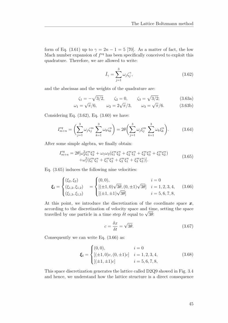
The Lattice Boltzmann method
form of Eq. (3.61) up to γ = 2n − 1 = 5 [70]. As a matter of fact, the lowMach number expansion of f eq has been specifically conceived to exploit thisquadrature. Therefore, we are allowed to write:
Iγ =3∑j=1
ωjζγj , (3.62)
and the abscissas and the weights of the quadrature are:
ζ1 = −√
3/2, ζ2 = 0, ζ3 =√
3/2; (3.63a)
ω1 =√π/6, ω2 = 2
√π/3, ω3 =
√π/6. (3.63b)
Considering Eq. (3.62), Eq. (3.60) we have:
Ieqm+n =
( 3∑j=1
ωjζmj
3∑k=1
ωkζnk
)= 2θ
( 3∑j=1
ωjξmj
3∑k=1
ωkξnk
). (3.64)
After some simple algebra, we finally obtain:
Ieqm+n = 2θ[ω22ξm1 ξ
n2 + ω1ω2(ξm1 ξ
n2 + ξm2 ξ
n1 + ξm2 ξ
n3 + ξm3 ξ
n2 )
+ω21(ξm1 ξ
n1 + ξm1 ξ
n3 + ξm3 ξ
n1 + ξm3 ξ
n3 )].
(3.65)
Eq. (3.65) induces the following nine velocities:
ξi =
(ξ2, ξ2)
(ξ1,2, ξ1,2)
(ξ1,3, ξ1,3)
=
(0, 0), i = 0
[(±1, 0)√
3θ, (0,±1)√
3θ] i = 1, 2, 3, 4,
[(±1,±1)√
3θ] i = 5, 6, 7, 8,
(3.66)
At this point, we introduce the discretization of the coordinate space x,according to the discretization of velocity space and time, setting the spacetravelled by one particle in a time step δt equal to
√3θ:
c =δx
δt=√
3θ. (3.67)
Consequently we can write Eq. (3.66) as:
ξi =
(0, 0), i = 0
[(±1, 0)c, (0,±1)c] i = 1, 2, 3, 4,
[(±1,±1)c] i = 5, 6, 7, 8,
(3.68)
This space discretization generates the lattice called D2Q9 showed in Fig. 3.4and hence, we understand how the lattice structure is a direct consequence
45

Chapter 3
1
2
33
4
56
87
0
Figure 3.4. D2Q9 lattice structure
of the quadrature formula we have chosen and the constraint imposed by thepreservation of the moments up to third order. Via a similar procedure otherappropriate lattices can be derived such as the D3Q27 in three dimensions.Moreover, it should be noted that, according to this space discretization, thespeed of sound of the model cs, which as already mentioned in Subsec. 3.53is equal to
√θ, is related to c by:
cs =c√3
=1√3
δx
δt. (3.69)
Actually, it is common practice in literature to assume the space step δx andthe time step δt to be unity. In this case we will talk of “lattice units” andobviously in this system of unit cs = 1/
√3.
According to Eqs. (3.65) and (3.66), if we consider a generic polynomialof degree k + 2, like in Eq (3.58), we have:
Ieqk = 2θ
[ω2
1ψk(ξ0) +4∑i=1
ω1ω2ψk(ξi) +8∑i=5
ω21ψk(ξi)
]. (3.70)
The comparison between Eq. (3.70) and Eq. (3.58), allows to evaluate theweights Wi introduced in Eq. (3.58) as:
Wi = 2πθ exp
[ξ2i
2θ
]wi, (3.71)
where,
wi =
4/9, i = 0,
1/9, i = 1, 2, 3, 4,
1/36, i = 5, 6, 7, 8.
(3.72)
Taking into account the weights of Eq. (3.71), we introduce the weightedmass distribution functions fi:
fi(x, t) = Wif(x, ξi, t), (3.73)
46

The Lattice Boltzmann method
and consequently according to Eq. (3.58), the moments f can be computedas a sum over the fi of the related polynomial ψk(ξi):
Ik =8∑i=0
ψk(ξi)fi. (3.74)
It is easy to verify that the equilibrium distribution function of the weightedfi is given by:
f eqi (x, t) = Wifeq(x, ξi, t) = ρwi
[1 +
3ξi · uc2
+9(ξi · u)2
2c4− 3u2
2c2
]. (3.75)
Finally, we are able to derive the Lattice Boltzmann equation. In fact, wehave to consider Eq. (3.51) for the discrete velocity ξi and multiply it for therelated weight Wi:
fi(x+ ξiδt, t+ δt)− fi(x, t) = −1
τ(fi(x, t)− f eqi (x, t)), i = 0, 1, . . . , 8,
(3.76)which is known as the BGK Lattice Boltzmann equation.
After this derivation, an analysis of Eq. (3.76) and how it was obtainedis certainly needed. We see that the Lattice Boltzmann equation is a simpleand explicit scheme, despite its complex origin. Basically the concept ofcollision and streaming introduced for the LGA in Sec. 3.1 are inherited bythe Lattice Boltzmann method, but applied to the distribution functions.We can enlist the key steps of the LBM algorithm:
1. At t=0, the lattice is initialised by means of suitable distribution func-tions dependent on the particular problem we are dealing with. Forexample, if density ρ and velocity u are known, the simplest way is toset initial fi(x, 0) at equilibrium, using Eq. (3.75). For more details onthe initialization procedures see [71].
2. The collision term J(fi) = −1/τ(fi−f eqi ) on the right side of Eq. (3.76)is evaluated on each lattice site and for each velocity, of course.
3. The post-collision value of fip in x can now be computed as fip(x, t) =fi(x, t) + J(fi).
4. The fip of the node x are simply streamed along the relative connectednodes fi(x+ ξiδt, t+ δt) = fip(x, t).
5. Now, in each node, we can compute ρ and u, and, thus the new equi-librium distribution functions and start again from point 2.
47

Chapter 3
Actually, the issue of boundary conditions in LBM has been voluntarily over-looked thus far, since we will talk about it later on.
Thus, the LBM shares the inherent parallelization typical of LGA. Thecollision term is evaluated locally and so it does not need communication atall, while the streaming step is just a shift operation.
Furthermore, it is clear that LBM are inherently transient solvers. There-fore, we cannot simulate a steady state directly, but it will be always viewedas the limit of a related transient problem. In general, we need to define anappropriate parameter in order to understand whether the steady state canbe considered reached or not.
Differently from other conventional CFD scheme such as Finite VolumeMethods [72] in the Lattice Boltzmann methods we witness the coupling be-tween velocity and coordinate spaces, which forces the grid structure to havea certain degree of symmetry. Thus, we are not allowed to construct arbi-trary structured meshes, but it is possible to realize a local grid refinement[73, 74], though this possibility will not be explored in this thesis. However,LBM proves to be surprisingly accurate and also guarantees an easy handle,when dealing with complex geometries [73] and, for this reason, they are verysuited for flow in porous media.
In Subsec. 3.7.2 we have touched on the issue of the sound speed in theLattice Boltzmann methods (see also [75, 76] ). As a matter of fact, in themodel presented we are considering an isothermal process and thus, the speedof sound is equal to the derivative of pressure with respect to density at con-stant temperature cs = (∂P/∂ρ)T =
√θ. This assumption is fundamental in
order to obtain the regular lattice structure induced by Eq. (3.66) and with-out it, we could not be able to obtain the numerical method itself. If θ isnot kept constant, we will draw just a weird model, without physical mean-ing. Nevertheless, as we know, sound waves are basically adiabatic and theisothermal case is an unlikely situation. Consequently, if we want to use theLBM with BGK collision term, for simulations of compressible flows, we haveto deal with this isothermal speed of sound, instead of the most appropriateisentropic one. However, if we want to simulate an incompressible flow weare not interested in compressibility effects and sound waves, but we want tokeep them as limited as possible, indeed. In fact, similarly to other compress-ible schemes [77], in order to approximate the incompressible Navier-Stokesequations, the Mach number should be very low, since it is the parameterthat governs the compressibility effects. In particular, as pointed out in [78],LBM with BGK recovers compressible Navier-Stokes equation, which in turnare used to approximate an incompressible flow with an error O(Ma2) on thecontinuity equation and O(Ma3) in the momentum equations.
The Lattice Boltzmann equation with BGK collision term suffers some
48

The Lattice Boltzmann method
drawbacks due to the BGK approximation. In particular, the simulated gasshows a fixed Prandtl number (equal to 1) and a fixed ratio between shearand bulk viscosity [29]. Moreover, it can be proved that the BGK LBEcoupled with the usual Bounce-Back boundary conditions on walls, that wewill introduce later on, produces a slip velocity dependent on the relaxationparameter τ [79]. In the context of incompressible flows in porous media, thisimplies that permeability does not remain constant and becomes dependenton viscosity ν, simply because the geometry representation varies with τ . Infact, we will show in Chap. 4 that the viscosity of the model is given by:
ν = c2s
(2τ − 1
2
)δt =
2τ − 1
6
δx2
δt, (3.77)
and it follows necessarily that τ > 1/2, in order to obtain a positive viscosity.
3.8 The Multiple-Relaxation-Time model
The main reason for the shortcomings of the BGK model presented in Sub-sec. 3.7.3 is the single relaxation parameter of the collision term. As a matterof fact, with a single relaxation time constant, we cannot tune independentlythe macroscopic transport coefficients, such as bulk and shear viscosities.In order to increase the number of tunable coefficients, we definitely needmore relaxation parameters. The Multiple-Relaxation-Time (MRT) modelhas been introduced for the first time in [28] and its aim is to overcome themain deficiencies of the BGK model.
Let us consider a general Lattice Boltzmann model defined by a set of Nvelocities ξi where i = 0, 1, . . . , N − 1, connecting each lattice node to itsneighbours, and the corresponding distribution functions fi. Obviously,also a set of equilibrium distribution functions is defined f eqi , dependingon the the local conserved quantities as usual. In the most generic case, theevolution equation is given by:
|f(x+ ξδt, t+ δt)〉 − |f(x, t)〉 = − ¯S[|f(x, t)〉 − |f eq(x, t)〉], (3.78)
where we have used the ket notation | 〉 to denote column vectors, while thebra notation 〈 | will be used to denote row vectors; ¯S represents a collisionmatrix, whose eigenvalues are all between 0 and 2 in order to attain linearstability [28]. Within this framework, the BGK model can be regarded as aspecial case of the MRT model, in which ¯S = ω ¯I, where ¯I is the identitymatrix and ω = 1/τ is called the relaxation frequency. As a matter of fact,the constraint on linear stability for the BGK model is actually a request forpositive viscosity.
49

Chapter 3
However, in the MRT model, the collision step is basically carried outin the space of moments of the distribution function, and the relaxation pa-rameters corresponds to relaxation frequencies towards equilibrium of certain“hydrodynamic modes”. In order to understand the previous statement weneed to examine in depth the concept of moments introduced in Subsec. 3.7.3.
In continuous kinetic theory a moment of order n of f is a tensor of rankn defined as [80]:
In(x, t) =
∫ξ. . .ξ︸ ︷︷ ︸n times
f(x, ξ, t) dξ. (3.79)
It is easy to recognize that the number of independent components of amoment of order n, in a D-dimensional space, is given by the combina-tion with repetition of D element taken n times, that is equal to CD,n =(D + n− 1)!/[(D − 1)!n!]. Thus, in 2D it is equal to n + 1. For the sake ofsimplicity, from now on we will consider the 2-dimensional case.
However, in discrete kinetic theory, the moments are computed as a sumover a specific set of N velocities ξi [80]
In(x, t) =N−1∑i=0
ξi. . .ξi︸ ︷︷ ︸n times
fi(x, t). (3.80)
In general, we can view a component of a moment of order n Iγ1...γn as thescalar product between the column vector of the distribution function |f〉and a N -dimensional row vector 〈mγ1...γn|, characteristic of the elementarymoment considered. Hence:
Iγ1...γn = 〈mγ1...γn|f〉 , (3.81)
where the components of 〈mγ1...γn| are obviously of the form ξmx ξly with m+
l = n. Hence, the moment Mγ1...γn is basically represented by a vector ofRN . Now we can extend the definition of moment, considering also linearcombination of elementary moments, i.e., the polynomial, and consequentlythe moment space M ≡ RN . The number of independent discrete momentsis therefore equal to N . It is obvious now that, regardless of the velocitieschosen, if N < n + 1, the correct model will not be able to represent themoments up to order n, since the independent moments would be differentfrom the continuous one. However, this is just a necessary condition torepresent the continuous moments correctly, but it is very useful becausefor instance, it allows to say immediately that a 2-dimensional model with3 velocities cannot be able to recover the Navier-Stokes equation, since inSubsec. 3.7.3 we required the preservation of moments up to third order.
50

The Lattice Boltzmann method
Let us consider the lattice D2Q9. For this discrete model we can choosethe following elementary independent moments [81]. The first four momentsare the collision invariants:
m′1 = ρ =8∑i=0
fi, (3.82a)
m′2 = ρux = jx =8∑i=0
ξixfi, (3.82b)
m′3 = ρuy = jy =8∑i=0
ξiyfi, (3.82c)
m′4 = ρ(e+1
2u2) =
8∑i=0
(ξ2ix + ξ2
iy)fi. (3.82d)
As we know, pressure P is defined as the arithmetic mean of the diagonalstresses, i.e., in 2-dimensions P = 1/2(σxx + σyy) = 1/2(
∑i ξ
2ixfi +
∑i ξ
2iyfi).
Thus, we define the diagonal deviatoric components of the stress tensor aspxx,yy = σxx,yy−P =
∑i 1/2(ξ2
ix,y−ξ2iy,x)fi, while the off-diagonal components
are pxy = σxy = pyx = σyx. We can add two independent moments related tothe stress tensor to those of Eqs. (3.82):
m′5 = 2pxx =8∑i=0
1
2(ξ2ix − ξ2
iy)fi, (3.83a)
m′6 = pxy =8∑i=0
ξixξiyfi. (3.83b)
In fact, we can consider as independent moments only the one between sxxand syy, because from the moments of Eqs. (3.82), we can compute thepressure P , by means of the state equation Eq. (3.33), and therefore sxx andsyy are not independent.
As m′7 and m′8 we set the energy fluxes along x, y of the kinetic energycorresponding to ξx,y:
m′7 = φxy =8∑i=0
ξixξ2iyfi, (3.84a)
m′8 = φyx =8∑i=0
ξiyξ2ixfi. (3.84b)
Finally, we set the last independent moment
m′9 = ε =8∑i=0
ξ2ixξ
2iyfi, (3.85)
51

Chapter 3
that can be regarded as a higher order energy transport term [81].Thus, we denote with 〈η′j| the vectors in the moment space M, corre-
sponding to the moments of Eqs. (3.82), (3.83), (3.84) and (3.85). For thelattice D2Q9 they are given by:
¯M ′ =
〈η′1|〈η′2|〈η′3|〈η′4|〈η′5|〈η′6|〈η′7|〈η′8|〈η′9|
=
〈ρ|〈jx|〈jy|
〈ρ(e+ 1/2u2)|〈2pxx|〈pxy|〈φxy|〈φyx|〈ε|
=
1 1 1 1 1 1 1 1 10 1 0 −1 0 1 −1 −1 10 0 1 0 −1 1 1 −1 −10 1 1 1 1 2 2 2 20 1 −1 1 −1 0 0 0 00 0 0 0 0 1 −1 1 −10 0 0 0 0 1 −1 −1 10 0 0 0 0 1 1 −1 −10 0 0 0 0 1 1 1 1
(3.86)
Although these vectors are independent, they are not orthogonal. In or-der to obtain orthogonal vectors 〈ηj|, we have to apply the Gram-Schmidtprocedure, which, taking as starting vector 〈ρ|, yields:
¯M =
〈η1|〈η2|〈η3|〈η4|〈η5|〈η6|〈η7|〈η8|〈η9|
=
〈ρ|〈jx|〈jy|〈e|〈2pxx|〈pxy|〈qx|〈qy|〈ε|
=
1 1 1 1 1 1 1 1 10 1 0 −1 0 1 −1 −1 10 0 1 0 −1 1 1 −1 −1−4 −1 −1 −1 −1 2 2 2 20 1 −1 1 −1 0 0 0 00 0 0 0 0 1 −1 1 −10 −2 0 2 0 1 −1 −1 10 0 −2 0 2 1 1 −1 −14 −2 −2 −2 −2 1 1 1 1
(3.87)
Let us denote with ηj the moment identified by the vector in moment space|ηj〉, i.e., ηj = 〈mj|f〉 and with |η〉 the corresponding row vector. Accordingly,we can write:
|η〉 = ¯M |f〉 → |f〉 = ¯M−1 |η〉 . (3.88)
Thus, there is a linear relationship between the vector of moments |η〉 andthe vector of the distribution functions |f〉, described by the matrix ¯M . Atthis point the idea is to consider a particular collision matrix ¯S (introducedin Eq. (3.78)), such that its eigenvectors are the row vectors of ¯M . In thisway, the collision step can be carried out in the moment space, by means of
52

The Lattice Boltzmann method
a diagonal collision matrix¯S:
δρδjxδjyδe
δ2pxxδpxyδqxδqyδε
=
sρ 0 0 0 0 0 0 0 00 sjx 0 0 0 0 0 0 00 0 sjy 0 0 0 0 0 00 0 0 se 0 0 0 0 00 0 0 0 spxx 0 0 0 00 0 0 0 0 spxy 0 0 00 0 0 0 0 0 sqx 0 00 0 0 0 0 0 0 sqy 00 0 0 0 0 0 0 0 sε
ρ− ρeqjx − jeqxjy − jeqye− eeqpxx − peqxxpxy − peqxyqx − qeqxqy − qeqyε− εeq
(3.89)
Now we have to represent this collision in terms of the distribution functionsusing Eq. (3.88) and finally, the Lattice Boltzmann equation for the MRTmodels turns into:
|f(x+ ξδt, t+ δt)〉 − |f(x, t)〉 = − ¯M−1 ¯S[|f(x, t)〉 − |f eq(x, t)〉], (3.90)
where the equilibrium moments can be computed by means of the equilibirum
distribution function introduced in Eq. (3.75). The parameters of¯S are
now related to the “hydrodynamic modes”, which possess a macroscopicmeaning and, clearly, we can set sρ = sjx = sjy = 0, since ρ, jx and jy arepreserved during a collision. Tuning the six parameters left, we are able toset the various transport coefficients. In fact, as shown in [29], if we setspxx = spxy = sν = 1/τ , the viscosity of the model has exactly the sameexpression of Eq. obtained for the BGK model, but we are allowed to controlalso the bulk viscosity ζ, which is determined by se = sζ :
ζ =2
9(
1
sζ− 1
2). (3.91)
Moreover, the parameters of the MRT model can be properly chosen in orderto achieve optimal stability [41] or to attain a well-defined no-slip conditionwhen using the Bounce-Back rule [82].
53


Chapter 4
The Chapman-Enskogexpansion
In this chapter, we will initially discuss how the forcing term can be in-cluded in the Lattice Boltzmann equation, analysing different methods. Af-terwards, the Chapman-Enskog procedure will be applied to the BGK LatticeBoltzmann equation with the forcing term, in order to restore the Navier-Stokes equations. At the end of this procedure, the relationship betweenthe macroscopic coefficients and the relaxation parameter will be definitelyclear. Moreover, we will be able to show the error sources. In our analysis,we will generally refer to Kuzmin’s work [1], but the Chapman-Enskog pro-cedure will be applied to a more general case than the one considered in [1],providing insights on the correct way of including the forcing term.
4.1 The role of δt
Let us write again the Lattice Boltzmann equation introduced in Sec. 3.7,that is Eq. (3.76)
fi(x+ ξiδt, t+ δt)− fi(x, t) = −1
τ(fi(x, t)− f eqi (x, t)), i = 0, 1, . . . , N − 1.
The starting point of the Chapman-Enskog expansion is the assumption ofconvective scaling, δt ∼ δx, which introduces a precise relationship betweenδx and δt. From Eqs. (3.68), we realize that under this assumption thediscrete velocities ξi are kept constant during the scaling.
The consequence of the convective scaling is that for the Lattice Boltz-mann equation, the role of the Knudsen number, introduced in Sec. 3.5, canbe carried out by δt. However, this assumption is not trivial. In fact, atfirst sight, it seems straightforward that for δt→ 0 the solution is fi → f eqi .However, in Subsec. 3.7.1, we have seen that actually τ = λ/δt, where λ
55

Chapter 4
is the relaxation parameter of the continuous BGK Boltzmann equation 1.Consequently, the right side of Eq. (3.76) goes to zero when δt→ 0, withoutnecessarily requiring that fi → f eqi . To solve this contradiction, we need todraw an analogy with the continuous Boltzmann BGK equation. Basically,since the LBE is a discretization of the BE, in order to recover the Navier-Stokes equations we need to be in the same conditions, which allow thisrecovery starting from the BE, that is, the low Knudsen number condition.As shown in [1], the Knudsen number for the BGK collision term Kn ∼ λ.Accordingly, we need to assume that δt ∼ Kn ∼ λ. In this way, τ = λ/δtremains constant in this procedure, and thus we are allowed to say that whenτ → 0, fi → f eqi . However, we will see at the end of this derivation that theseassumptions on the Chapman-Enskog expansion applied to the LBE may becontroversial. For this reason, in literature, different methods to recover theNavier-Stokes equations from the LBE have been attempted, which will bebriefly discussed in the last section of this chapter.
In what follows, we will perform the Chapman-Enskog expansion aroundthe solution f eq, taking δt as the parameter of the expansion. In addition,we will denote ε = δt in order to highlight that it is the small parameter ofthe perturbative method.
4.2 Inclusion of the forcing term
The inclusion of external or internal forces into the Lattice Boltzmann equa-tion is carried out adding the term εFi:
fi(x+ ξiε, t+ ε)− fi(x, t) = −1
τ(fi(x, t)− f eqi (x, t)) + εFi. (4.1)
The idea behind this additional term is that it should be proportional to ε; infact if we consider a collision in a finite time ε in presence of forces, accordingto Newton’s second law, the total momentum will change proportionally toε.
In the second instance, in the case of external forces, the force functionsFi should be constructed so that the macroscopic forcing term is equal toF = ρa as in Eqs. (3.38). As a matter of fact, in this process we go throughan opposite direction with respect to what we have done so far, namely wedesign the mesoscopic dynamics starting from the macroscopic one. Thisdoes not happen with the Boltzmann equation, in which the forcing termemerges naturally from the conservation equations. In a certain sense startingfrom the Boltzmann equation, we derive the macroscopic equations and,
1It should be noted that in lattice units λ = τ since δt = 1 in this system of units
56

The Chapman-Enskog expansion
consequently, the expression of the forcing term, and then we impose toobtain the same term in the LBE conservation equations. Also the presenceof an hypothetical mass source M can be handled with Fi, as we will see inwhat follows.
However, the generation of the forcing term could be not only caused bythe force functions Fi, but also by the collision term, redefining the densityand momentum used in the computation of f eqi [83].
From the previous observations, we recognize that what really matters isthat in mass and momentum equations:
εM−∑i
fiτ
+∑i
f eqiτ
= εM, (4.2a)
εFα −∑i
ξiαfiτ
+∑i
ξiαfeqi
τ= εFα, (4.2b)
where M =∑
i Fi and Fα =∑
i ξiαFi are moments of Fi. Thus:
εM− ρ
τ+ρeq
τ= εM, (4.3a)
εFα −ρuατ
+ρequeqατ
= εFα. (4.3b)
We will prove that within this framework, the macroscopic density and mo-mentum, which take part in the restoration of macroscopic equations are:
ρm = ρ+ εM
2, (4.4a)
ρmumα = ρuα + εFα2, (4.4b)
where “m” stands for macroscopic. Three specific cases are worth mentioning[1]
1. ρ = ρeq, ρequeqα = ρuα : the forcing term is only due to the moments ofFi (scheme I);
2. ρeq = ρm, ρequeqα = ρmumα : the forcing term is distributed between themoments of the collision term and the moments of Fi (scheme II);
3. ρeq = ρ + εMτ , ρequeqα = ρuα + εFατ : the forcing term is generatedonly by the moments of the collision term (scheme III).
Actually, we will prove that the correct model is the second one, which isthat proposed by Guo in [84]. Only with this model, ρm and ρmumα represent
57

Chapter 4
properly the macroscopic density and momentum into the recovered Navier-Stokes equations, while the others introduce additional sources of error. Inaddition, we identify the third method as the method of shifting velocityproposed by Shan & Chen in [4]. In this paper an interaction force is intro-duced between particles, in order to allow phase separation. We will explainin details the Shan-Chen model in Chap. 7, but for now we have to keep inmind that it introduces the forcing term by means of scheme III.
4.3 The Chapman-Enskog multi-scale expan-
sion
The first step of the Chapman-Enskog procedure for the LBE is the Taylorexpansion of the left side of Eq. (4.1):
fi(x+ ξiε, t+ ε)− fi(x, t) =+∞∑n=0
(∂t + ξiβ∂β)n
n!εnf(x, t), (4.5)
where we have used the notation ∂t to denote the partial derivative withrespect to time t, and ∂β to denote the partial derivative with respect to thecoordinate xβ.
The Chapman-Enskog expansion is a multiscale method in which boththe unknown function fi and the time variable are expanded as a polynomialin the small parameter ε. For ε → 0 the solution is obviously f eqi , which isour known solution. Hence, fi and t are expanded as follows:
fi = f(0)i + εf
(1)i + ε2f
(2)i + · · · =
+∞∑k=0
εkf(k)i , (4.6a)
t = t0 + εt1 + ε2t2 + · · · =+∞∑k=0
εktk, (4.6b)
and accordingly
∂t = ∂t0 + ε∂t1 + ε2∂t2 + · · · =+∞∑k=0
εk∂tk . (4.7)
Thus, the time derivative of a generic function g will be given by ∂tg =∂t0g+ ε∂t1g+ ε2∂t2g+ . . . . According to the previous statements f
(0)i = f eqi .
The insertion of Eqs. (4.5) and (4.6) into Eq. (4.1) gives:
+∞∑n=0
(∑∞
k=0 εk∂tk + ξiβ∂β)n
n!εn(f
(0)i +εf
(1)i +ε2f
(2)i +. . . ) = −
∑+∞n=1 ε
nf(n)i
τ+εFi.
(4.8)
58

The Chapman-Enskog expansion
4.4 Restoration of macroscopic equations
Let us introduce an approximation of order n of Eq. (4.8), considering termsof order at most εn. In particular, we are interested in approximations oforder ε1 and ε2 (the approximation of order ε0 is trivial) for which it is easyto verify the following results:
ε1 : (∂t0 + ξiβ∂β)f(0)i = −f
(1)i
τ+ Fi, (4.9a)
ε2 : ∂t1f(0)i + (∂t0 + ξiβ∂β)f
(1)i +
(∂t0 + ξiβ∂β)2f(0)i
2= −f
(2)i
τ. (4.9b)
It is worth pointing out that these successive approximations are not affectedby errors. In fact, we can simply assume that f
(1)i and f
(2)i satisfy respectively
Eq. (4.9a) and Eq. (4.9b), and in general f(k)i satisfies the approximation of
order εk. It is easy to verify that this procedure is consistent, since if thesesuccessive equations hold, the Lattice Boltzmann equation is consequentlysatisfied. In general, within the Chapman-Enskog framework, the momentsof f can be also viewed as an expansion in ε. For example, considering ρ andρuα:
ρ =∑i
fi =∑i
f(0)i + ε
∑i
f(1)i + ε2
∑i
f(2)i + · · · =
ρ(0) + ερ(1) + ε2ρ(2) + . . . ,
(4.10a)
ρuα =∑i
ξiαfi =∑i
ξiαf(0)i + ε
∑i
ξiαf(1)i + ε2
∑i
ξiαf(2)i + · · · =
ρ(0)u(0)α + ερ(1)u(1)
α + ε2ρ(2)u(2)α + . . . ,
(4.10b)
A direct consequence of Eqs. (4.2) is that ρ and ρu are certainly due only to
f(0)i and f
(1)i . Hence, we can write Eqs. (4.2) as:
ρ = ρ(0) + ετ(M−M), (4.11a)
ρuα = ρ(0)u(0)α + ετ(Fα − Fα), (4.11b)
which by comparison with Eqs. (4.10) allows to identify
ρ(1) = τ(M−M) (4.12a)
ρ(1)u(1)α = τ(Fα − Fα), (4.12b)
and consequently:
ρ = ρ(0) + ερ(1), (4.13a)
ρuα = ρ(0)u(0)α + ερ(1)u(1)
α . (4.13b)
59

Chapter 4
It is obvious that direct consequences of Eqs (4.13) are∑
i f(k)i = 0 and∑
i ξiαf(k)i = 0 for k ≥ 2.
The macroscopic equations we would like to obtain via the Chapman-Enskog expansion are those of a compressible and Newtonian fluid, in whichthe relationship between stresses and velocities (or better their gradients) isgiven by:
σαβ = −[µ(∂uα∂xβ
+∂uβ∂xα
) + δαβ(ζ∂uγ∂xγ− P )
], (4.14)
where µ and ζ are respectively the dynamic and bulk viscosities; δαβ is theKronecker delta. In Eq. (4.14) we have assumed the conventions induced byEqs. (3.38). In this case the Navier-Stokes equations we want to restore are:
∂tρ+ ∂α(ρuα) = M, (4.15)
∂t(ρuα) + ∂β(ρuβuα) = −∂αP + ∂β(µ∂βuα) + ∂β((µ+ ζ)∂αuβ) + Fα. (4.16)
In Eq. (4.15) we have also considered a mass source term, due for exampleto a chemical reaction.
4.4.1 Mass equationLet us consider the Lattice Boltzmann equation in the ε1 approximationEq. (4.9a). By summing over i and taking into account Eqs. (4.12) it is easyto derive:
ε1 : ∂t0ρ(0) + ∂α(ρ(0)u(0)
α ) = M. (4.17)
The same operations applied to the ε2 approximation Eq. (4.9b) yields:
∂t1ρ(0) + ∂t0ρ
(1) + ∂α(ρ(1)u(1)α ) +
∑i
(∂t0 + ξiα)2f(0)i
2= 0. (4.18)
The insertion of Eq. (4.17) into Eq. (4.18) leads to:
∂t1ρ(0) + ∂t0ρ
(1) + ∂α(ρ(1)u(1)α ) +
∑i
(∂t0 + ξiα)(−f(1)i
τ+ Fi)
2= 0. (4.19)
After some simple algebra and remembering the definitions of M and Fαgiven in Sec. 4.2, Eq. (4.19) finally turns into:
ε2 : ∂t1ρ(0) +
(1− 1
2τ
)∂t0ρ
(1) +
(1− 1
2τ
)∂α(ρ(1)u(1)
α )+
1
2∂t0M+
1
2∂αFα = 0.
(4.20)
60

The Chapman-Enskog expansion
Multiplying Eq. (4.20) by ε and summing it with Eq. (4.17) we obtain:
∂t0
(ρ(0) + ε
(1− 1
2τ
)ρ(1) + ε
M2
)+
∂α
(ρ(0)u(0)
α + ε
(1− 1
2τ
)ρ(1)u(1)
α + εFα2
)+ ε∂t1ρ
(0) = M,
(4.21)
which taking into account Eqs. (4.11) and (4.12) becomes:
∂t0
(ρ+ ε
M
2
)+ ∂α
(ρuα + ε
Fα2
)+ ε∂t1ρ
(0) = M. (4.22)
At this point, we would like to adopt the second order approximation in ε ofthe time derivative ∂t = ∂t0 + ε∂t1 +O(ε2), in order to obtain the derivativeof a macroscopic density with respect to time. Clearly, the only correct wayis to set ρ(0) = ρm = ρ + εM/2, that is the method denoted as scheme II.With this assumption, no further sources of errors are introduced. Of coursewe identify also ρmumα = ρuα + εFα/2 and finally we obtain:
∂tρm + ∂α(ρmumα ) = M +O(ε2). (4.23)
However, from Eqs. (4.3) and (4.4), we notice that we can write:
ρeq = εM(τ − 1
2)− τεM+ ρm. (4.24)
This means that by summing and subtracting the term εM(τ − 1/2)− τεMinto Eq. (4.22) we can obtain:
∂tρm + ∂α(ρmumα ) = M − ε∂t1(εM(τ − 1
2)− τεM) +O(ε2). (4.25)
We notice that the additional source of error is due a partial derivative withrespect to the time scale t1, which is rigorously zero, if the mass source M andthe the zero-th order moments of M of Fi do not depend on time. Anywayscheme II is definitely the most appropriate. Furthermore, we notice that theadditional source of error shows a dependency on the relaxation parameterτ . Similar considerations can be found in the paper of Guo et al. [84].
4.4.2 Momentum EquationNow our goal is to obtain the macroscopic momentum equation. Basicallythe procedure is similar to that adopted in Subsec. 4.4.1, but the derivationis lengthier and more complex. In particular new sources of error will arise.
61

Chapter 4
Thus, let us consider the equation for ε1 Eq. (4.9a). Multiplying it by ξiαand summing over i we obtain:
ε1 : ∂t0(ρ(0)u(0)α ) + ∂β
(∑i
ξiαξiβf(0)i
)= Fα, (4.26)
where we have also used Eq. (4.12b). The same procedure applied to Eq. (4.9b)yields:
ε2 : ∂t1(ρ(0)u(0)α ) +
(1− 1
2τ
)∂t0(ρ(1)u(1)
α ) +
(1− 1
2τ
)∂β
(∑i
ξiαξiβf(1)i
)+
1
2∂t0Fα +
1
2∂β
(∑i
ξiαξiβFi
)= 0.
(4.27)The multiplication of Eq. (4.27) by ε and its summation to Eq (4.26) gives:
∂t0
(ρ(0)u(0)
α + ε
(1− 1
2τ
)ρ(1)u(1)
α +ε
2Fα)
+ ε∂t1(ρ(0)u(0)α )+
∂β
(∑i
ξiαξiβf(0)i + ε
(1− 1
2τ
)∑i
ξiαξiβf(1)i +
ε
2
∑i
ξiαξiβFi
)= Fα.
(4.28)Using Eqs. (4.11) and (4.12) we finally obtain:
∂t0
(ρuα +
ε
2Fα)
+ ε∂t1(ρ(0)u(0)α )+
∂β
(∑i
ξiαξiβf(0)i + ε
(1− 1
2τ
)∑i
ξiαξiβf(1)i +
ε
2
∑i
ξiαξiβFi
)= Fα.
(4.29)In analogy with Subsec. 4.4.1 we recognize that the most reasonable wayto introduce the approximation ∂t = ∂t0 + ε∂t1 + O(ε2) is to set ρ(0)u
(0)α =
ρmumα = ρuα + εFα/2. It is easy to verify that assuming ρeq = ρm andρequeqα = ρmumα , the zeroth and first order moments of Fi shall satisfy:∑
i
Fi = M
(1− 1
2τ
), (4.30a)
∑i
ξiαFi = Fα
(1− 1
2τ
). (4.30b)
Hence, we are allowed to write:
∂t(ρmumα ) + ∂β
(∑i
ξiαξiβf(0)i + ε
(1− 1
2τ
)∑i
ξiαξiβf(1)i +
ε
2
∑i
ξiαξiβFi
)= Fα +O(ε2).
(4.31)
62

The Chapman-Enskog expansion
Again, the considerations made for the mass equation in Subsec. 4.4.2 are thesame for the momentum equation. In fact, if we did not set ρ(0)u
(0)α = ρmumα ,
we would obtain an additional source of error and Eq. 4.31 would become:
∂t(ρmumα ) + ∂β
(∑i
ξiαξiβf(0)i + ε
(1− 1
2τ
)∑i
ξiαξiβf(1)i +
ε
2
∑i
ξiαξiβFi
)= Fα − ε∂t1(εFα(τ − 1
2)− τεFα) +O(ε2).
(4.32)
Similarly to the mass equation, these terms are rigorously zero, if Fα and Fαdo not depend purely on time. However, we will see that also other sourcesof error arise if ρ(0)u
(0)α 6= ρmumα .
We notice that in Eq. (4.31), higher order moments of f(0)i , f
(1)i and Fi
begin to come up and their computation will be the main problem in whatfollows.
Thus, we have to derive the expression of these moments in terms ofmacroscopic density and velocity. In particular, let us focus on the momentsof f
(1)i . According to Eq. (4.9a) we can write f
(1)i as:
f(1)i = τ(Fi − ∂t0f
(0)i − ξiγ∂γf
(0)i ). (4.33)
Accordingly, the second order moment of f(1)i , which appears in Eq. (4.31),
can be expressed in terms of the moments of f(0)i and Fi as:∑
i
ξiαξiβf(1)i = τ
(∑i
ξiαξiβFi − ∂t0∑i
ξiαξiβf(0)i − ∂γ
∑i
ξiαξiβξiγf(0)i
).
(4.34)Consequently Eq. (4.31) turns into:
∂t(ρmumα ) + ∂β
[∑i
ξiαξiβFi + ε
(τ − 1
2
)(∑i
ξiαξiβFi−
∂t0∑i
ξiαξiβf(0)i − ∂γ
∑i
ξiαξiβξiγf(0)i
)+ε
2
∑i
ξiαξiβFi
]= Fα +O(ε2).
(4.35)It is now explained the reason why in Subsec. 3.7.3 we required the quadra-ture formula to preserve the moments of the low Mach number expansion ofthe Maxwellian up to third order. In fact, we notice that in Eq. (4.35) a third
order moment of f(0)i appears and we would like to compute it correctly. Ac-
tually, as properly explained in Appendix A.2, these moments correspondsto those of a Maxwellian neglecting the terms of order O(Ma3). This isintuitive indeed, as the Maxwellian distribution function is expanded up to
63

Chapter 4
second order in the Mach number and thus, the expansion is characterizedby an error O(Ma3). As shown in Appendix A.2, the second and third order
moments of f(0)i are given by:∑
i
ξiαξiβf(0)i = δαβc
2sρ
(0) + ρ(0)u(0)α u
(0)β , (4.36a)∑
i
ξiαξiβξiγf(0)i = c2
sρ(0)(δαβu
(0)γ + δαγu
(0)β + δβγu
(0)α ). (4.36b)
Even in this case we realize the importance of setting ρm = ρ(0) and ρmumα =
ρ(0)u(0)α , otherwise we would obtain additional errors. For example, let us
consider the case of scheme III, that is the method of shifting velocity in theequilibrium distribution function [4]. For the sake of simplicity, let us alsoconsider M = 0 in this example, which means that ρ = ρm = ρeq. In thiscase, it is easy to obtain from Eqs. (4.3) and (4.4) that:
ueqα = umα +εFαρ
(τ − 1
2
). (4.37)
Now, if we insert the previous relationship into the equation of the secondorder moments, Eq. (4.36a), we obtain:∑
i
ξiαξiβf(0)i = δαβc
2sρ+ ρ
[umα +
εFαρ
(τ − 1
2
)][umβ +
εFβρ
(τ − 1
2
)].
(4.38)It is clear that extra sources of error arise if we do not set umα = ueqα . Huanget al. have shown that these additional terms may play an important role,especially when dealing with multi-phase flows [85]. Thus, from now on we
will set ρ(0) = ρm and u(0)α = umα .
The insertion of Eqs. (4.36) into Eq. 4.35 yields:
∂t(ρmumα ) + ∂β
(δαβc
2sρm + ρmumα u
mβ
)+ ε
(τ − 1
2
)∂β
∑i
ξiαξiβFi−
∂t0(δαβc2sρm + ρmumα u
mβ )− ∂γ(c2
sρm[δαβu
mγ + δαγu
mβ + δβγu
mα )]
+
∂β
(ε
2
∑i
ξiαξiβFi
)= Fα +O(ε2).
(4.39)
Let us focus on the following terms:
∂β∂t0(c2sδαβρ
m) = c2s∂α∂t0ρ
m = c2s∂α(M − ∂γρmumγ ), (4.40)
where we have inserted Eq. 4.17.
64

The Chapman-Enskog expansion
In addition:
∂β∂t0(ρmumα umβ ) = ∂β[umα ∂t0(ρmumβ ) + umβ ∂t0(ρmumα )− umα umβ ∂t0ρm] =
= ∂βumβ [Fα − ∂α(c2sρm)− ∂γ(ρmumα umγ )]+
umα [Fβ − ∂β(c2sρm)− ∂γ(ρmumβ umγ ]− umα umβ [M − ∂γ(ρmumγ )],
(4.41)
neglecting the terms of order O(u3), i.e., O(Ma3), we finally obtain:
∂β∂t0(ρmumα umβ ) = ∂β[(umα Fβ + umβ Fα)−
c2s(u
mα ∂βρ
m + umβ ∂αρm)− umα umβM ] +O(Ma3).
(4.42)
Thus, we have introduced a further source of error related to the Mach num-ber. This approximation is necessary indeed, because, as it was previouslymentioned, in the low Mach number expansion of the Maxwellian we are notcapable of recovering the terms of third or higher order in Ma.
The last term we analyse is:
∂β∂γ[c2sρm(δαβu
mγ + δαγu
mβ + δβγu
mα )] =
= ∂β[c2s(ρ
m∂βumα + umα ∂βρ
m)] + ∂β[c2s(ρ
m∂αumβ + umβ ∂αρ
m))] + ∂α[c2s∂α(ρmumγ )].
(4.43)The substitution of these terms into Eq. 4.39 gives:
∂tρmumα + ∂α(c2
sρm) + ∂β(ρmumα u
mβ ) + ετ∂β
(∑i
ξiαξiβFi
)−
ε
(τ − 1
2
)∂α[c2
s(M − ∂γ(ρmumγ ))]− ∂β[(umα Fβ + umβ Fα)−
c2s(u
mα ∂βρ
m + umβ ∂αρm)− umα umβM ]− ∂β[c2
s(ρm(∂βu
mα + ∂αu
mβ )+
umα ∂βρm + umβ ∂αρ
m)]− ∂α[c2s∂γ(ρ
mumγ )]
= Fα +O(ε2) +O(Ma3).
(4.44)
At this point, we neglect the term ε(τ−1/2)∂β(umα umβM) that isO(Ma2)O(ε).
It should be noted that this term is rigorously zero if M = 0. Moreover, wealso set a further constraint on Fi:
τ∂β
(∑i
ξiαξiβFi
)=
(τ − 1
2
)[∂α(c2
sM)] + ∂β(umα Fβ + umβ Fα), (4.45)
so that these terms cancel each other out into Eq. (4.44). Thus, the Fi shouldsatisfy Eqs. (4.30) and (4.45) and it can be shown that these constraints arefulfilled by [1]:
Fi = wi
(1− 1
2τ
)(M +
F · ξic2s
+ξiαξiβ − c2
sδαβ2c4s
Fαuβ
). (4.46)
65

Chapter 4
As a consequence, Eq. (4.44) turns into:
∂t(ρmumα ) + ∂β(ρmumα u
mβ ) = −∂α(c2
sρm) + ∂β
[ε
(τ − 1
2
)c2sρm∂βu
mα
]+
∂β
[ε
(τ − 1
2
)c2sρm∂αu
mβ
]+ Fα +O(ε2) +O(Ma3) +O(Ma2)O(ε).
(4.47)The comparison between Eq. (4.47) and Eq. (4.16) allows the identificationof the dynamic viscosity of the model:
µ = ε
(τ − 1
2
)c2sρm, (4.48)
which was already anticipated in Subsec. 3.7.3. Therefore, the viscosity de-pends on the following parameters:
• the time step size δt and the spatial step size δx, since c2s ∼ δx2/δt2;
• the relaxation parameter τ ;
• the lattice model, which defines the proportionality constant betweencs and δx/δt (for the D2Q9 it is 1/
√3).
Finally, the BGK Lattice Boltzmann method recovers the following momen-tum equation:
∂t(ρmumα ) + ∂β(ρmumα u
mβ ) = −∂α(c2
sρm) + ∂β(µ∂βu
mα )+
∂β(µ∂αumβ ) + Fα +O(ε2) +O(Ma3) +O(Ma2)O(ε).
(4.49)
Comparing again Eq. (4.49) to Eq. (4.16), it is clear that the BGK modelpredicts a zero bulk viscosity (assuming the definition given in Eq. (4.14)).
From Eq. (4.48), we clearly see the problem of the Chapman-Enskogexpansion applied to the LBE. In fact, at the beginning of the procedure wehave pointed out that, in order to ensure a mathematical consistency of themethod, we need to assume τ = λ/δt = const, along with the assumptionof convective scaling δx ∼ δt. This means that when δt → 0, also µ → 0.Thus, by means of the Chapman-Enskog expansion, we have actually shownthat the LBE is able to recover the compressible Navier-Stokes equation inthe limit of low viscosity. In order to obtain more general results, differentmethods have been proposed in literature, which will be briefly described inthe next section.
As a concluding remark, it is worth pointing out that in this procedurethe effect of boundary conditions has not been taken into account.
66

The Chapman-Enskog expansion
4.5 Beyond the Chapman-Enskog expansion
By means of the Chapman-Enskog expansion, the Lattice Boltzmann equa-tion is able to recover the macroscopic Navier-Stokes equations. However,we have also pointed out that this procedure is based on the assumption ofconvective scaling δt ∼ δx and in addition, it is rigorously valid in the limitof low viscosity. This has lead to employ different methods to recover theNavier-Stokes equation from the LBE.
Junk [86] identified the diffusive scaling δt ∼ δx2 as the natural choice forthe analysis of the LBE. However, even this method is based on an asymp-totic analysis. Holdych et al. [87] attempted to recover the Navier-Stokesequations without requiring a further relationship between its parameters, inorder to obtain a general order of convergence of the methods. In particular,these parameters are τ, δx and δt, but they are not independent because ofthe viscosity relationship Eq. 3.8. In addition, in [87], no asymptotic anal-ysis are employed in this procedure. In this case, considering δx and δt asthe independent parameters in the viscosity relationship Eq. 3.8, the error ofthe LBE in the continuity equation, denoted by C.E. (Continuity Error) andmomentum equation, denoted by M.E. (Momentum Error) should be givenin the O notation and in the incompressible limit by:
C.E. = O(δx4) +O(δt2) +O((δt/δx)2), (4.50a)
M.E. = O(δx2) +O(δt2) +O((δt/δx)2), (4.50b)
where δt/δx is clearly proportional to Ma. This result has been obtainedin [87] without considering the presence of a forcing term and the influenceof boundary conditions. The details of the sources of error can be found in[87]. In the case of diffusive scaling δt ∼ δx2 it is clear that the error on thecontinuity equation and the momentum equation becomes both O(δx2).
67


Chapter 5
Boundary conditions in LBM
As for any other numerical method, boundary conditions play a key role forthe success of Lattice Boltzmann methods. Boundary conditions are neededto solve any partial differential equation, and they are supposed to model theinteraction between the system and the external environment. Thus, it is notsurprising that also Lattice Boltzmann methods require boundary conditions,as in Chap. 3 we have shown in details how the Lattice Boltzmann equationcan be viewed as a special discretization of the Boltzmann equation.
In this chapter, initially, the answer to the question “what do boundaryconditions mean for LBM?” is provided, analysing also the different philoso-phies of boundary conditions.
Then, we will analyse the Bounce-Back rule, which is the most widelyused scheme to model the interaction with solid boundaries for its simplicityof coding. In particular, some drawbacks of the Bounce-Back rule, whenused together with the BGK model, are shown. These shortcomings areparticularly annoying for porous media applications and should be carefullytackled.
The periodic boundary conditions are also presented, because they willbe used in the numerical simulations.
Afterwards, we will focus on the issue of imposing macroscopic quantities,such as pressure and velocity, on a boundary node. A general and rathersimple analysis inspired by Bennett’s work [88] will help us to understandwhich macroscopic quantities shall be imposed simultaneously and which not.In this framework, we will present the Zou-He boundary conditions, whichhave proved to be very efficient especially for the 2D case.
69

Chapter 5
y
x13
5
8
6
7
2
4
INLET OUTLET
Figure 5.1. Inlet node of a two-dimensional channel with the D2Q9 lattice model.The red arrows identify the velocities, whose distribution functions are unknown.
5.1 Meaning of boundary conditions in LBM
In order to understand what boundary conditions mean in Lattice Boltzmannmethods, let us refer to the D2Q9 lattice model and let us consider an inletnode of a two-dimensional channel, as shown in Fig. 5.1. It is clear that aftera streaming process in this node the distribution functions f0, f2, f3, f4, f6 andf7 are known, while f1, f5 and f8, which come from the external environment,are still to be determined. Thus, what boundary conditions do in LBMis nothing but providing a rule, i.e., a set of equations, to determine theincoming distribution functions. Obviously, similar considerations can bedrawn for outlet nodes and wall nodes.
From the macroscopic point of view, we are certainly allowed to statethat in LBM, boundary conditions have not got a straightforward physicalmeaning. In conventional fluid dynamics, where the Navier-Stokes equationsare solved directly, boundary conditions regard pressure and velocity, whichtake part to the equations. In LBM, instead, boundary conditions for theunknown distribution functions need to be prescribed.
From an analysis of the different schemes proposed in literature, a cate-gorisation into two broad categories of boundary conditions is suggested:
• Boundary conditions which try to model the interaction between thegas and external environment. The Bounce-Back scheme, described inthe following section, and reflection schemes, such as the one proposedin [89], belong to this category.
• Boundary conditions which try to translate the macroscopic conditionsin terms of the distribution functions. We number among this categorythe Inamuro boundary condition [26], the finite difference scheme pro-posed by Skordos [25], the regularized boundary dynamics developed
70

Boundary conditions in LBM
by Latt [27] and the aforementioned Zou-He method [24].
It is worth pointing out that methods such as those proposed by Latt andSkordos do not prescribe only the unknown distribution functions, but theyprovide a new value to all the fi at the boundary node. Moreover, all thesemethods are developed for straight boundaries, while in practical problemswe may deal with curved boundaries. In this case, the rigid lattice structureof LBM represents a drawback indeed, because we are not free to adapt themesh to the geometry as it happens with finite volume methods. For this rea-son, interpolation or extrapolation methods are needed for these boundaries.Examples of boundary conditions for curved boundaries are the schemes pro-posed by Mei et al. in [90] and by Bouzidi et al. in [91].
5.2 Wall interaction: the Bounce-Back rule
The Bounce-Back rule is a scheme supposed to model the interaction betweenthe gas and the solid wall boundary. The idea behind this rule is rather simpleand also suggested by the name itself: particles in these nodes reverse theirvelocities and are reinjected into the fluid domain.
From this basic idea, several Bounce-Back schemes have come out [22].Here, we will focus only on the one used in this thesis. This scheme isillustrated in Fig. 5.2 and it is translated mathematically by the followingequation:
fq(xb, t+ δt) = f ∗q (xb, t), (5.1)
where xb is the coordinate vector of a fluid node bordering a Bounce-Backnode; q denotes a generic inward distribution function, while q its outwardcounterpart; the symbol ∗ means that the distribution function is evaluatedafter the collision step.
In Fig. 5.2, the Bounce-Back nodes are the black ones. They shall not beconsidered as fluid nodes, but “logic” nodes, indeed. When a particle try toaccess these nodes through a natural streaming process, they are reinjectedinto the fluid domain according to the aforementioned rule.
Thus, the Bounce-Back rule is certainly a very simple to code and this isits main strong point.
5.2.1 Geometry dependency on relaxation parametersThough its simplicity of coding, the Bounce-Back rule does not lack draw-backs and the main one is certainly a slip-velocity dependent on the relax-ation parameters of the model. If we consider a two-dimensional Hagen-Poiseuille flow and we assume that the wall is placed half-way between thelast fluid node and the Bounce-Back node, the slip velocity at the wall is
71

Chapter 5
f4 f8f7
(a) Time t: before collision
f ∗4 f ∗8f ∗7
(b) Time t: after collision
f2 = f ∗4 f5 = f ∗7f6 = f ∗8
(c) Time t+ δt
Figure 5.2. Sketch of the Bounce-Back process for a bottom wall node: during thestreaming step, the unknown inward distributions f2, f5 and f6 are set equal to thepost-collision value of the distributions related to the opposite outward velocities,i.e. f∗4 , f
∗7 and f∗8
72

Boundary conditions in LBM
given by [92]
Us =1
4
(8
sq− 8− sν
2− sν
)Gδt, (5.2)
where G = |∇p|/ρ, sν and sq are the relaxation parameters of the MRT modeldefined in Sec. 3.8. The slip velocity of different Bounce-Back schemes areproperly analysed in [79]
From Eq. (5.2), it is clear that in general the Bounce-Back rule does notyield a zero slip velocity at the wall, which is what we would like to obtainin case of an incompressible flow. The velocity is actually zero somewherebetween the last fluid node and the Bounce-Back node, but this position isfunction of sν and sq. Hence, the geometry of the system varies with sν andsq.
In porous media applications, this is a very annoying drawback, indeed.In fact, the permeability of a porous media, which is its main physical quan-tity, is function of the geometry only for Stokes flow, and consequently itis dependent on the relaxation parameters. Therefore, the value of the re-laxation parameters shall be carefully tuned in order to obtain a low slipvelocity at the half-way wall.
It is worth noting that Eq. (5.2) is valid in case of Hagen-Poiseuille flowand it is not general. However, it is good practice to take Eq. (5.2) asreference and to tune the relaxation parameters accordingly.
As we know from Sec. 3.8, the BGK model can be viewed as a MRTmodel with all the relaxation parameters equal to ω. In this case, Eq. (5.2)turns into:
Us =1
4
(ω2 − 16ω + 16
ω(2− ω))
)Gδt =
48ν2 − 1
8νGδt, (5.3)
where we recall that ν = (1/ω − 1/2)/3. Thus, in this case, the condi-tion which gives a zero slip velocity is ν2 = 1/48, corresponding to ω =1, 071796 . . . and τ = 1/ω = 0.9330127 . . . . In general it is good practice tochoose ω approximately 1.
The MRT model allow us to tune the parameters so that Us is alwayszero. This condition is obviously fulfilled when:
sq =8(2− sν)
8− sν, (5.4)
which gives rise to the so-called Two-Relaxation-Time (TRT) model [30]: allthe parameters are equal to sν , except for sq given by Eq. (5.4). Hence, theTRT model allows more freedom in the choice of viscosity.
Anyway, if the refinement is carried out by means of a diffusive scaling inwhich δt ∼ δx2, from Eq. (5.2) it is straightforward that also Us ∼ δx2 and
73

Chapter 5
thus, the effect of this drawback rapidly decrease when δx→ 0 independentlyfrom the choice of sν and sq.
As a concluding remark of this section, let us analyse the reason of thenon-zero slip velocity provided by the Bounce-Back scheme. In Sec. 5.1 wehave included the Bounce-Back rule into the category of boundary conditionsthat do not prescribe a macroscopic quantity at the relative node, but try tomodel the interaction with the external environment (in this case the wall).Thus, it is not surprising that the velocity is actually not zero. However, itis shown in [93], and also reported in [82], that the slip velocity of a gas isgiven by:
Us = σKnH∂yu|w, (5.5)
where σ is a coefficient dependent on the model of interaction between gasparticles and wall; H is the height of the channel; Kn is the Knudsen numberthat for an ideal gas is proportional to the ratio between Mach and Reynoldsnumbers:
Kn ∼ Ma
Re=
ν
Hcs. (5.6)
Hence, taking into account Eqs. (5.3), (5.5) and (5.6), two remarks shouldbe pointed out:
• the velocity of a gas at wall is never exactly zero;
• the velocity of a gas at wall increases with Kn and thus with ν, asit happens for the slip velocity predicted by the Bounce-Back scheme(5.3), though the law is different.
Accordingly, we conclude that the slip velocity due to the Bounce-Backscheme shows common features with the real slip velocity of an ideal gas,since the BB rule somehow tries to model the wall-gas interaction.
5.3 Periodic boundary conditions
The periodic boundary conditions are very simple and should be appliedwhen the system is periodic in one or more directions. In general in this kindof problems we are able to identify an elementary geometry which repeatsitself infinite times. Thus, the study of the whole system reduces to the studyof this fundamental cell.
Let us focus on Fig. 5.3. The periodic boundary conditions for the upperand lower boundary are represented by the following equations:
f7(xu, t) = f7(xl, t), f4(xu, t) = f4(xl, t), f8(xu, t) = f8(xl, t), (5.7a)
f5(xl, t) = f5(xu, t), f2(xl, t) = f2(xu, t), f6(xl, t) = f6(xu, t), (5.7b)
74
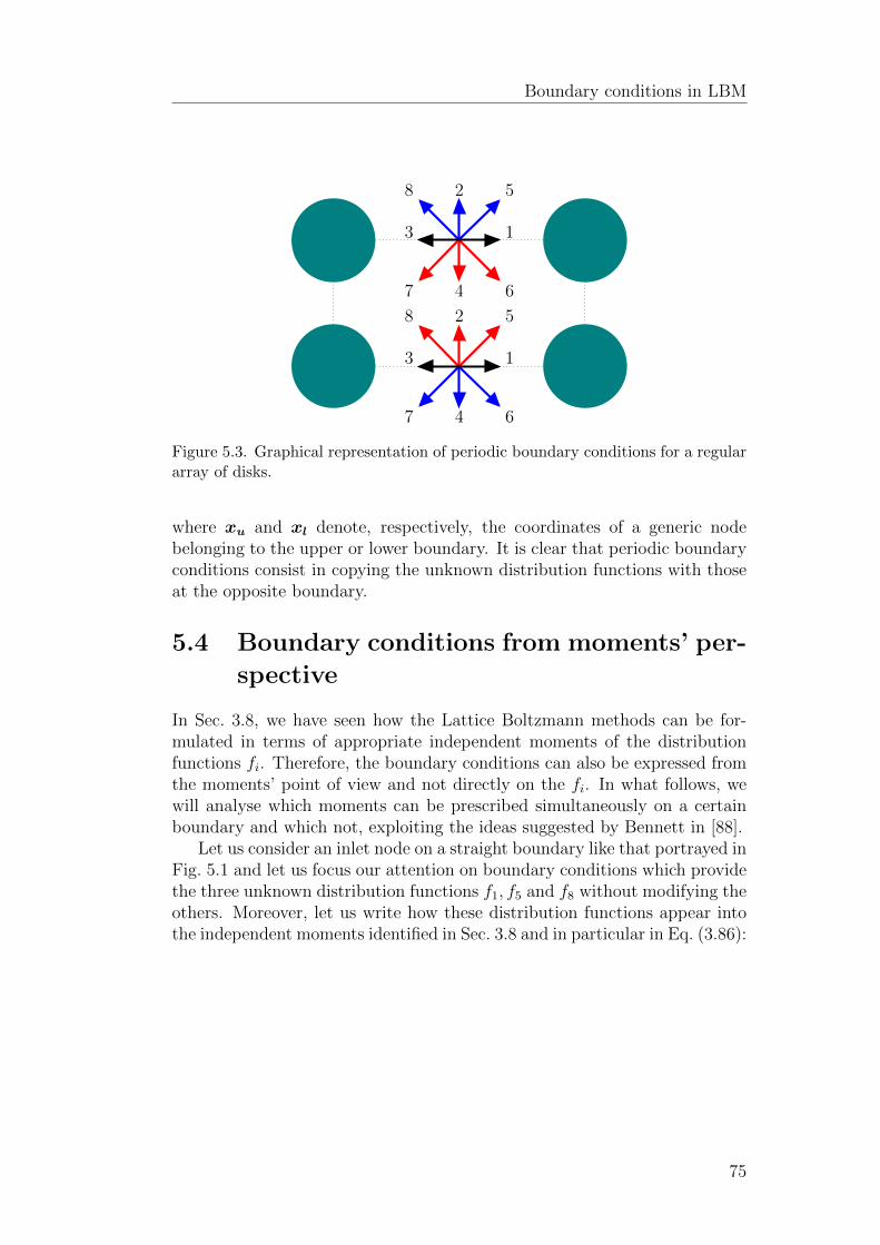
Boundary conditions in LBM
1
2
3
4
5
67
8
1
2
3
4
5
67
8
Figure 5.3. Graphical representation of periodic boundary conditions for a regulararray of disks.
where xu and xl denote, respectively, the coordinates of a generic nodebelonging to the upper or lower boundary. It is clear that periodic boundaryconditions consist in copying the unknown distribution functions with thoseat the opposite boundary.
5.4 Boundary conditions from moments’ per-
spective
In Sec. 3.8, we have seen how the Lattice Boltzmann methods can be for-mulated in terms of appropriate independent moments of the distributionfunctions fi. Therefore, the boundary conditions can also be expressed fromthe moments’ point of view and not directly on the fi. In what follows, wewill analyse which moments can be prescribed simultaneously on a certainboundary and which not, exploiting the ideas suggested by Bennett in [88].
Let us consider an inlet node on a straight boundary like that portrayed inFig. 5.1 and let us focus our attention on boundary conditions which providethe three unknown distribution functions f1, f5 and f8 without modifying theothers. Moreover, let us write how these distribution functions appear intothe independent moments identified in Sec. 3.8 and in particular in Eq. (3.86):
75

Chapter 5
ρ→ f1 + f5 + f8, (5.8a)
jx → f1 + f5 + f8, (5.8b)
jy → f5 − f8, (5.8c)
ρ(e+ 1/2u2)→ f1 + 2(f5 + f8), (5.8d)
2pxx → f1, (5.8e)
pxy → f5 − f8, (5.8f)
φxy → f5 + f8, (5.8g)
φyx → f5 − f8, (5.8h)
ε→ f5 + f8. (5.8i)
Analysing these dependencies it is very easy to realize which set of momentscannot be imposed simultaneously. For example, it is clear that it is notpossible to set both density ρ, i.e., pressure, from Eq. (3.34), and the x-component of momentum density jx, because they fix the value of the groupf1 + f5 + f8, while it is possible to set ρ and jy. For this reason, we are notallowed to fix pressure and the velocity vector at the same time.
Moreover, it is not sufficient to provide ρ and jx, for example, becausea further independent equation is needed in order to define f1, f5 and f8
univocally. This additional equation might regard another moment or itmight be just a modelling equation, as it happens with the Zou-He boundaryconditions which we will be describing in the following section.
5.5 Zou-He boundary conditions
In what follows, we will refer directly to the original paper of Zou and He[24], in which this kind of boundary condition appeared for the first time.
Let us consider again the inlet node of Fig. 5.1. We will analyse the caseof pressure boundary condition, in which the density ρ is imposed, while thecomponent of the velocity parallel to the surface, in this case uy, is set tozero. Let us write the equations for ρ, ρux and ρuy:
ρ = f0 + f1 + f2 + f3 + f4 + f5 + f6 + f7 + f8,
ρux = f1 − f3 + f5 − f6 − f7 + f8,
ρuy = f2 − f4 + f5 + f6 − f7 − f8.
(5.9)
Gathering together the unknown distributions and setting uy = 0, we obtain:
76
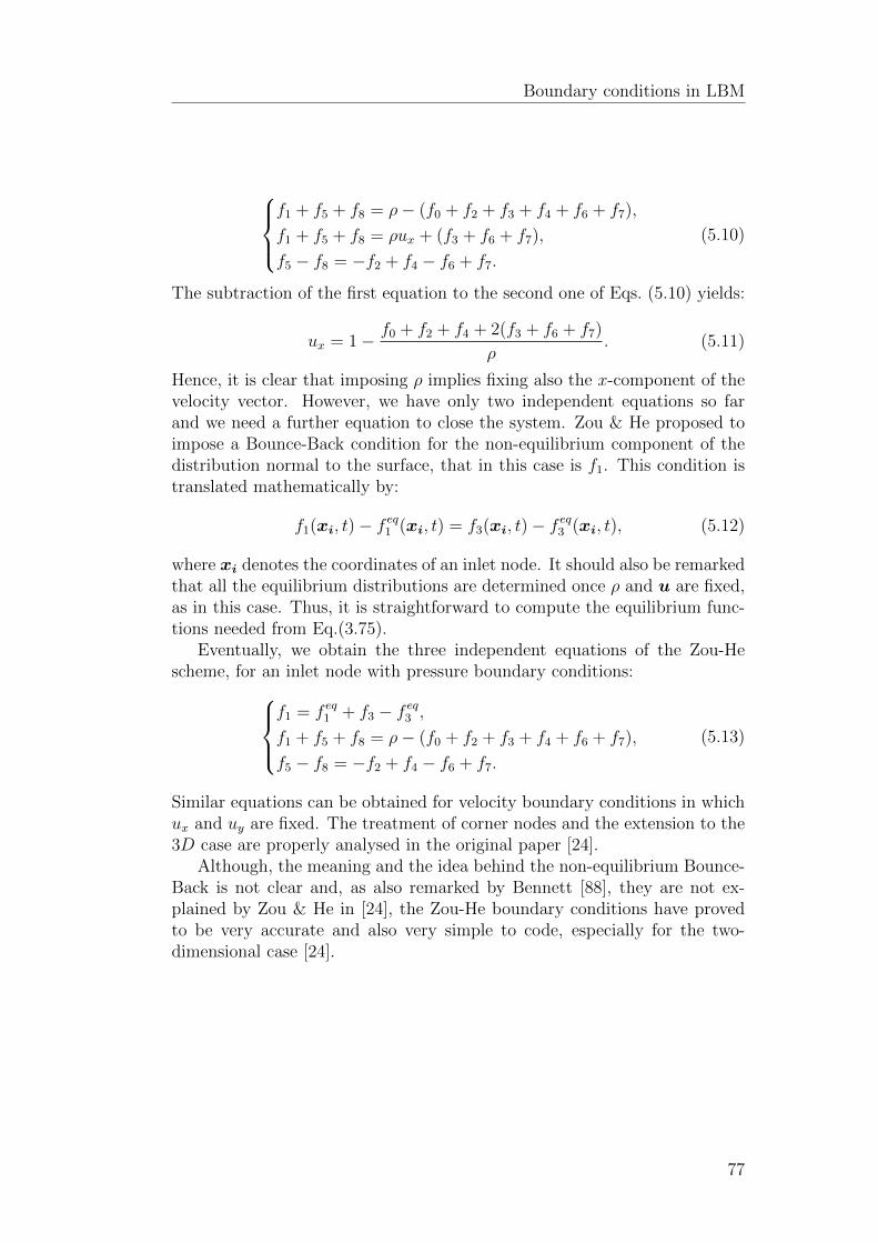
Boundary conditions in LBM
f1 + f5 + f8 = ρ− (f0 + f2 + f3 + f4 + f6 + f7),
f1 + f5 + f8 = ρux + (f3 + f6 + f7),
f5 − f8 = −f2 + f4 − f6 + f7.
(5.10)
The subtraction of the first equation to the second one of Eqs. (5.10) yields:
ux = 1− f0 + f2 + f4 + 2(f3 + f6 + f7)
ρ. (5.11)
Hence, it is clear that imposing ρ implies fixing also the x-component of thevelocity vector. However, we have only two independent equations so farand we need a further equation to close the system. Zou & He proposed toimpose a Bounce-Back condition for the non-equilibrium component of thedistribution normal to the surface, that in this case is f1. This condition istranslated mathematically by:
f1(xi, t)− f eq1 (xi, t) = f3(xi, t)− f eq3 (xi, t), (5.12)
where xi denotes the coordinates of an inlet node. It should also be remarkedthat all the equilibrium distributions are determined once ρ and u are fixed,as in this case. Thus, it is straightforward to compute the equilibrium func-tions needed from Eq.(3.75).
Eventually, we obtain the three independent equations of the Zou-Hescheme, for an inlet node with pressure boundary conditions:
f1 = f eq1 + f3 − f eq3 ,
f1 + f5 + f8 = ρ− (f0 + f2 + f3 + f4 + f6 + f7),
f5 − f8 = −f2 + f4 − f6 + f7.
(5.13)
Similar equations can be obtained for velocity boundary conditions in whichux and uy are fixed. The treatment of corner nodes and the extension to the3D case are properly analysed in the original paper [24].
Although, the meaning and the idea behind the non-equilibrium Bounce-Back is not clear and, as also remarked by Bennett [88], they are not ex-plained by Zou & He in [24], the Zou-He boundary conditions have provedto be very accurate and also very simple to code, especially for the two-dimensional case [24].
77


Chapter 6
Porous Media applications
In this chapter, we will start to get familiar with the Lattice Boltzmannsimulations from a practical point of view, carrying out simulations for severalgeometries. In particular, we will deal with the issue of setting appropriatesimulation parameters, keeping in mind the results of the previous chapters.For this reason, an accurate analysis of the error of the simulations willbe given, comparing different types of collision models, different schemesof boundary conditions and also two ways of scaling the time and spatialsteps. In order to carry out these analyses, we definitely need to study fluiddynamics problems whose solution is already known or well approximated.
Our first study will be the two-dimensional Hagen-Poiseuille flow alreadypresented in Sec. 2.2. The reasons which have justified this choice are three-fold. First of all, the analytical solution of the flow is known and given byEqs. (2.8), hence, the analysis of the error is straightforward. In the secondinstance, in Sec. 2.4, we have seen how the Carman-Kozeny model is basedon the Hagen-Poiseuille equation, and thus this kind of flow plays an im-portant role in porous media. In general, we are allowed to say that flowin porous media at low Reynolds number shows common features with theHagen-Poiseuille flow and we can consider it as a preliminary reference case.Finally, in the LBM literature the flow in a two-dimensional straight channelis widely studied [79, 24, 94, 75, 95].
As a second test case, we will deal with a flow over a hexagonal andperiodic array of disks (or disks in 2D). This is a first example of porousmedium, whose study is simplified because of the periodic nature of theproblem, which allows us to consider only an elementary geometry and touse periodic boundary conditions. Even for this geometry, there exists someanalytical approximated formulas for permeability, so we can compare themwith the Lattice Boltzmann simulations, as well. This study takes inspirationfrom the works of Yadzchi et al. [96] and Pan et al. [35]. In the former, thestudy of the hexagonal array of disks is carried out using a finite element
79

Chapter 6
method, while in the latter LBM are used for a body-centred cubic array ofspheres.
Finally, we will analyse a porous medium made up of a random arrayof disks. For this geometry, the Lattice Boltzmann method will be usedmainly to verify the validity of the Carman-Kozeny model and to determinethe Reynolds number for which the flow does not obey the Darcy’s law anymore. In addition, the issue of “how to compute tortuosity” is addressed.
In Sec. 6.1, a general description of Palabos, the open source library usedto carry out the simulation is provided.
Before going into the results of the simulation, a detailed explanation ofthe simulation setup is provided, highlighting also the main difficulties in thisprocess. Throughout this chapter, for the sake of generality, we will alwaysuse dimensionless quantities.
6.1 The tool: Palabos
All the simulations in this thesis are carried out by means of Palabos. Palabosis an open-source library written in C++, specifically developed for Lat-tice Boltzmann methods. Palabos implements the main lattice models andboundary conditions, and its open-source nature allows also the developmentof new models to be embedded in its framework of functions and classes. Inthe current versions, Palabos lacks a graphical interface, and consequentlyalso the user needs to struggle with some programming. However, tutori-als and showcases are available for several topics, which definitely helps insetting up new problems.
The programming paradigm of Palabos is to exploit the inherent par-allelization of Lattice Boltzmann methods and at the same time to allowthe development of new models. In fact, by following some programmingrules, it is possible to write new Lattice Boltzmann schemes, without takingcare of the issue of parallelization of the code, which is done automatically.The main development guideline is that the new models, or in general newcontributions to the library, should be implemented by means of the func-tions and classes already present in the Palabos distribution, exploiting theobject-oriented structure of the library itself.
6.2 Simulation setup
First of all, let us introduce the concept of lattice units. It is a system ofunits which is very convenient in case of regular structures, like typical latticestructure of LBM. In this system the spatial step δx and the time step δt
80

Porous Media applications
are both set to unity, δx = δt = 1. Sometimes, it is also convenient to setthe density equal to unity at inlet, for example. Obviously, this establishes adirect correspondence between the mass in physical 1 or dimensionless unitsand the mass in lattice units, which is needed to convert the value of thedistribution functions. We will refer to this units of mass as mu in thischapter.
Thus, considering the case of the D2Q9 lattice shown in Fig. 3.4, thedistance between two neighbouring nodes in lattice units is equal to 1 or
√2,
and in addition, the number of iterations corresponds to the time in latticeunits. Usually, the simulations are carried out numerically using these units,and then the results are converted in dimensionless units and, eventually, inphysical units.
It is straightforward that in lattice units, the BGK Lattice Boltzmannequation Eq. (3.76) turns into:
fi(x+ ξi, t+ 1)− fi(x, t) = −1
τ(fi(x, t)− f eqi (x, t)), i = 0, 1, . . . , 8, (6.1)
where the discrete velocities ξi are of course given by Eqs. (3.68) with c =δx/δt = 1, and the equilibrium distribution functions f eqi are computed fromEq. (3.75) using quantities in lattice units.
From Eq. (3.69) and from Eq. (3.8), it is clear that in lattice units thespeed of sound cs and the kinematic viscosity ν are given by cs = 1/
√3 and
ν = (2τ − 1)/6. From now on we will denote the quantities in lattice unitswith the subscript “lu”.
Let us now focus our attention on the simulation setup. The simulationsshare the following five general features:
• the simulations are based on the lattice D2Q9;
• the steady state is assumed to be reached when the Value Tracer, anapproriate parameter defined in Palabos to detect the steady state, fallsbelow a user-defined value;
• the Bounce-Back rule described in Sec. 5.2 is used to model the gas-wall interaction. Accordingly, the geometry is provided simply in theform of a matrix of 0 and 1;
• constant pressure boundary conditions, like the Zou-He presented inSec. 5.5, are imposed at inlet and outlet. Thus, we follow the approachof fixing the ∆P and obtaining the Darcy’s velocity as a result of thesimulations;
1By physical units, we mean the International System of Units
81

Chapter 6
• at time t = 0 the flow is initialized with a linear pressure gradient, i.e., alinear density gradient, with ∆P between inlet and outlet equal to thatimposed by the boundary conditions when t ≥ 0; all the componentsof the velocity vector are initialized to zero. At t = 0, the distributionfunction fi are evaluated at equilibrium;
In addition, it is worth pointing out that we want to simulate incompressibleflows, using the Lattice Boltzmann method which is a compressible scheme.
In order to understand how to choose the parameters of the simulation,let us analyse the simple two dimensional Hagen-Poiseuille flow. As it wasstated before, throughout this chapter we would like to obtain results in di-mensionless units, as those introduced in Sec. 2.1, and therefore, the quantitywithout subscript are all intended as dimensionless. Let us suppose that wehave a grid of Nx = 51 and Ny = 52 lattice nodes. Obviously the upperand lower nodes are Bounce-Back nodes, and in Sec. 5.2, we have seen inthis scheme that the wall is placed half-way between the last fluid node andthe Bounce-Back node. Thus, we are actually simulating a channel of heightHlu = 50 and length Llu = 50. We take as reference length the height of thechannel L0 = H and we obtain that the spatial step is δx = 1/H = 0.02.
As reference velocity, we need to relate a velocity to the ∆P imposedbetween inlet and outlet. From this velocity a Reynolds number is defined.In fact, in the opinion of the author, it would be awkward to compute theReynolds number directly during the post processing phase, since it would beaffected by error and it would depend on the parameters of the simulations,leading to a not univocally defined value. Hence, it is wise to establish areference velocity known ex ante the numerical simulations.
For the case of Hagen-Poiseuille flow the choice is rather natural, andwe set as reference velocity the Darcy’s velocity predicted by the analyticalsolution of the flow given in Eq. (2.10):
U0lu = − R2lu
3µlu
∆PluLlu
, (6.2)
where we remember that Rlu = Hlu/2. We will see in the following section,that a similar choice will be made for the case of the hexagonal and randomarray of disks.
It is also clear that assuming the reference density to be unity in latticeunits, it follows that µlu = νlu. The previous definitions allow to establisha direct correspondence between the Reynolds number and the ∆P if we fixthe spatial step and the kinematic viscosity in lattice units, ı.e., τ .
In fact, let us suppose that we want to simulate a flow with a givenReynolds number Re. The kinematic viscosity in dimensionless units is def-
82

Porous Media applications
initely ν = 1/Re, and the substitution into Eq. (3.8) yields:
δt = Re νlu δx2. (6.3)
If we fix the relaxation parameter τ , we finally obtain the time step in di-mensionless units δt. Accordingly, the reference velocity in lattice units isalso determined:
U0lu =δt
δx. (6.4)
Now, we can use Eq. (6.2) to compute the ∆P between inlet and outlet inlattice units and finally complete the simulation setup.
However, we have to take into account that the error of the Lattice Boltz-mann simulations is definitely associated also to the Mach number Ma givenby:
Ma =Ulucslu
=√
3δt
δx=√
3Re νlu δx. (6.5)
The Mach number shall always be taken under control, since it could affectthe results of the simulations. Thus, if the Mach number is considered toohigh we need to reduce either the δx or τ . Reducing the Reynolds number isin general not an option since it would change the problem. However, if weare interested in computing the permeability of a porous medium, we couldchange also the Reynolds number, as long as it is sufficiently low to preservethe validity of the Darcy’s law.
From the previous description, we realise that the simulation setup ofLattice Boltzmann simulations could be tricky and from the users’ point ofview, a little of experience is required. The following simulations will helpus to get familiar with this process.
6.3 Convective and diffusive scaling
In Sec. 4.5, we have seen how the sources of error δx, δt and Ma appearin the error formula for an incompressible flow Eq. (4.50). Furthermore, inChap. 4, we have carried out the Chapman-Enskog expansion whose startingpoint was the convective scaling δt ∼ δx.
However, two remarks should be emphasized for the convective scaling.First of all, since by definition δt/δx = const., during this scaling the Machnumber is kept constant, as well as the related error. Consequently, in theconvective scaling, we cannot achieve a perfect convergence. For this reason,it is wise to assume a sufficiently low Mach number at the beginning of thesimulations. In addition, if we consider Eq. (6.5) it is evident that if we wantto keep Ma constant, and also the Reynolds number constant during thescaling, when δx is decreased, it is necessary to increase the viscosity, namely
83

Chapter 6
0 20 40 60 80 100
0
10
20
30
40
50
60
70
80
90
100 0
0.3
0.6
0.9
1.2
1.4999
Figure 6.1. Velocity field of the Hagen-Poiseuille flow when the steady state isreached.
τ 2. Nevertheless, we have to take into account the additional problem ofthe slip velocity at wall, when we use Bounce-Back boundary conditions.For instance, for the BGK model we have seen in Subsec. 5.2.1 that Us isrigorously zero when τ = 0.9330127 . . . , and considering Eq. (5.3), duringthe convective scaling we shall keep under control the value of τ , which shallnot be much greater than unity.
Another possible scaling is the diffusive scaling, where δt ∼ δx2. In thiscase, also the Mach number tends to zero when δx → 0. The error of theLattice Boltzmann method becomes simply O(δx2). Unlike the convectivescaling, the diffusive scaling allow us to choose a fixed relaxation parameter τand keep also constant the Reynolds number. In fact, from Eq. (6.3) if we fixthe Reynolds number and the viscosity in lattice units, we obtain a diffusivescaling δt = a δx2, with a = Re νlu. Thus, we can choose τ minimizing forexample the slip velocity at wall, or from stability considerations.
The diffusive scaling guarantees a perfect convergence of the error, sinceall the sources of error approach zero. Nevertheless, the condition δt ∼ δx2
increases dramatically the number of iterations needed to reach the steadystate compared to the convective scaling.
6.4 Hagen-Poiseuille simulations
The Hagen-Poiseuille flow is investigated using three collision models:
2On the contrary, it should be remembered that we required a fixed τ in the Chapman-Enskog procedure, which lead to a variable viscosity.
84

Porous Media applications
1. the BGK model;
2. the TRT model we have described in Subsec. 5.2.1;
3. the Multiple-Relaxation-Time model with optimized stability intro-duced by Lallemand & Luo in [41]; this model makes use of the fol-lowing relaxation parameters: spxx = spxy = 1/τ , se = 1.63, sε = 1.14sqx = sqy = 1.92.
The Zou-He boundary conditions are used to impose pressure at inlet andoutlet. It would be interesting to analyse the error for different boundarycondition scheme, but we will tackle this issue for the case of hexagonal arrayof cylinders in Sec. 6.5. Before starting to comment the results, it is worthpointing out that all the figures are related to quantities in dimensionlessform, using as reference length the height of the channel H and as referencevelocity the average cross sectional velocity U0 obtained from Eq. (6.2).
Fig. 6.1 shows the visualization of the velocity field at the end of thesimulation, and it has been obtained using the BGK model with Nx = 101,Ny = 102, τ = 1 and Ma = 0.0001. In this figure, we can catch sight of thetypical parabolic profile of the Hagen-Poiseuille flow, as well as we notice thatthe maximum velocity is very close to the theoretical value of 1.5 predictedby Eq. (2.10).
Figs. 6.2 are obtained with the BGK model keeping fixed Ma = 0.0001and τ = 1. In this case, according to Eq. (6.5), the Reynolds number isinversely proportional to δx , Re ∼ 1/δx, and from Eq. (6.3) this leads toa convective scaling δt ∼ δx, with variable Reynolds number. The variationof the Reynolds number is not a great issue as long as the flow remainslaminar. In our simulations the maximum Reynolds number for δx = 1/25 isRe = 0.00866025 . . . , which is by far below the transition treshold of about2000. Thus, a convective scaling with variable Reynolds number and constantτ is acceptable in this case.
In Fig. 6.2, we are able to see how the parabolic profile of the Hagen-Poiseuille flow is well recovered even for a very coarse grid with Nx = 7 andNy = 8. This result is really helpful in case of porous media flow indeed.In fact, we know that the flow inside the pores of a porous medium sharescommon features with the Hagen-Poiseuille flow, and hence, we can establishas a general rule of thumb, that the distance between two walls in a porousmedium should be at least 5 or 6 lattice units, while about 13 lattice unitsshould be sufficient to ensure a good accuracy. Obviously, we have to keepthe Mach number sufficiently low.
Fig. 6.3 is realized with the same Mach number and τ as before, but withδx = 1/100. On the y-axis the absolute value of the local relative error ε isplotted on a logarithmic scale. We see that the order of magnitude of ε is
85

Chapter 6
−0.5 −0.4 −0.3 −0.2 −0.1 0 0.1 0.2 0.3 0.4 0.50
0.2
0.4
0.6
0.8
1
1.2
1.4
1.6
y
u(y
)
Numerical Solution
Analytical Solution
(a) δx = 1/6
−0.5 −0.4 −0.3 −0.2 −0.1 0 0.1 0.2 0.3 0.4 0.50
0.2
0.4
0.6
0.8
1
1.2
1.4
1.6
y
u(y
)
Numerical Solution
Analytical Solution
(b) δx = 1/13
−0.5 −0.4 −0.3 −0.2 −0.1 0 0.1 0.2 0.3 0.4 0.50
0.2
0.4
0.6
0.8
1
1.2
1.4
1.6
y
u(y
)
Numerical Solution
Analytical Solution
(c) δx = 1/25
Figure 6.2. Comparison between the analytical solution and the numerical resultsof the BGK model for different δx.
86

Porous Media applications
−0.5 −0.4 −0.3 −0.2 −0.1 0 0.1 0.2 0.3 0.4 0.510
−5
10−4
10−3
10−2
y
ε
Figure 6.3. Relative velocity error profile when δx = 1/100.
10−3 for nodes close to the wall, while it is 10−4 at the centre of the channel.The obvious reason is that near the wall there are greater gradients respectto the central region, which cause the error to increase. For our particularcase however, there is an additional explanation. As we know, when τ = 1,the BGK model coupled with the Bounce-Back rule does not guarantee azero slip velocity Us. The non-zero slip velocity causes an error which weighsdefinitely more close to the wall, where the velocities are lower.
Let us now focus our attention on the permeability dependency on τ . Inorder to show this dependency, we wish to carry out a numerical experimentin which the effect of Us is isolated from the other sources of error. Thenatural choice is to keep fixed the Mach number and the spatial step, and tosimulate the flow with different relaxation times. In this way, from Eq. (6.5),it follows that the product Re νlu must remain constant. Accordingly, weneed to accept a variation of the Reynolds number, which definitely doesnot change anything if the flow remains laminar. From Eq. (6.3), also theδt remains constant, and thus, all the sources of error in Eq. (4.50) are keptconstant.
Fig. 6.4 shows the trend of the relative error on permeability ∆k/kth =(k−kth)/kth with τ , for the three models. The permeability has been obtainedby computing the flow rate, and thus the Darcy’s velocity, by means of a mid-
87

Chapter 6
0.5 1 1.5 2−0.01
−0.005
0
0.005
0.01
0.015
0.02
0.025
τ
(k−
kth
)/k
th
BGK
TRT
MRT
Figure 6.4. Permeability dependency on τ for different collision models.
point rule for integration 3, and then using its definition given by the Darcy’slaw Eq. 2.14. We can see how the TRT model basically provides a constantpermeability as predicted by the theory. In addition, the BGK model exhibitsan error very close to zero when τ ≈ 0.9, which is again in agreement withthe theoretical results of Subsec. 5.2.1. The negative value of ∆k/kth forthe MRT model is due to the value of the relaxation parameter sq = 1.92assumed by this model. In fact, it is straightforward that the substitutionof this value into Eq. (5.2), yields a negative slip velocity in the range of τexamined in Fig. 6.4, that is a lower permeability than the case Us = 0.
In Fig. 6.5, we can see how this dependency is drastically reduced whenδx → 0. In particular, given a fixed τ , the scaling is carried out alwaysassuming a fixed Mach number (Ma = 0.0001), and in turn, a constantvalue of the product Re δx. Even in this case the global result is a convectivescaling δt ∼ δx.
As a concluding test for the Hagen-Poiseuille flow we will make a com-parison between the three models, in case of convective and diffusive scaling.We are able to see the results in Fig. 6.6. Differently from the previous cases,the convective scaling is carried out with a fixed Reynolds number and Machnumber. This means that we need to scale νlu ∼ 1/δx and consequently, τwill increase when δx is decreased. Obviously, we wish to keep the relaxation
3The error associated to this integration is O(δx2)
88

Porous Media applications
0.5 1 1.5 2−0.005
0
0.005
0.01
0.015
0.02
0.025
τ
(k−
kth
)/k
th
δ x= 0.04
δ x = 0.02
δ x = 0.01
Figure 6.5. Permeability dependency on τ for the BGK model, with different δx.
parameter low, not much greater than unity, or the error due to the slip ve-locity will take over. For this reason, we decide to choose a Mach number lowenough to guarantee that when δx is minimum, in this case δx = 1/200, therelaxation parameter is equal to one. Assuming that the Reynolds numberis fixed to Re = 0.1, this means Ma = 0.00014.
As it can be seen in Fig. 6.6(a), in case of convective scaling, the TRTmodel is definitely the model which shows the lowest relative error, while theMRT model performs worse than the BGK when δx is lower than 0.02, butbetter when it is greater.
The diffusive scaling setup is definitely simpler than the convective one.The relaxation parameter τ and the Reynolds number can be kept fixedduring the scaling. The simulations are carried out with τ = 1 and Re = 0.1.
According to Fig. 6.6(b), even for the diffusive scaling the best perfor-mances in terms of accuracy belong to the TRT model, while the MRT isdefinitely the one which produces the greater error for any δx.
As pointed out in Sec. 6.3, the error of the Lattice Boltzmann simulationswith diffusive scaling should be O(δx2). It is easy to verify this statementin our case. In fact, in Fig. 6.7, we can notice how the error of the diffusivescaling is well approximated by a parabolic function. This function has beenobtained using the Matlab function polyfit. In addition, Fig. 6.8 showsa comparison in logarithmic scale between the error on the permeabilityobtained with the diffusive scaling of the BGK model, and the curves in case
89

Chapter 6
0 0.01 0.02 0.03 0.04 0.05 0.06 0.07 0.080
1
2
3
4
5
6x 10
−3
δ x
|k−
kth
|/k
th
BGK
TRT
MRT
(a) Convective scaling
0 0.01 0.02 0.03 0.04 0.05 0.06 0.07 0.080
0.002
0.004
0.006
0.008
0.01
0.012
δ x
|k−
kth
|/k
th
BGK
TRT
MRT
(b) Diffusive scaling
Figure 6.6. Comparison of the relative error on permeability between the BGK,TRT and MRT, in case of diffusive and convective scaling.
90

Porous Media applications
0 0.01 0.02 0.03 0.04 0.05 0.06 0.07 0.080
1
2
3
4
5
6
7
8x 10
−3
δ x
|k−
kth
|/k
th
BGK
Parabolic fitting
Figure 6.7. Parabolic fitting of the error on permeability obtained with the BGKmodel by means of diffusive scaling.
the error is ∼ δx and ∼ δ2x. The error of the BGK model definitely follows
the curve with error ∼ δ2x, and thus, the BGK model shows a second order
accuracy in this case.Finally, Fig. 6.9 displays the comparison between the error produced by
the convective and diffusive scaling for the TRT model. In particular, thesame simulations are carried out for δx = 1/13, 1/25, 1/50, 1/100, 1/200. Thesimulations parameters are exactly the same for the coarser case, that isδx = 1/13. The Reynolds number is kept fixed in both cases to the valueRe = 0.1, while the relaxation parameter τ is constant only for the diffusivescaling, and it is chosen to be unity. From these values, it is easy to obtain theMach number when δx = 1/13: Ma = 0.00222058 . . . . Thus, the convectivescaling simulations are carried out using Re = 0.1 and Ma = 0.00222058 . . . .
The diffusive scaling performs definitely better in terms of accuracy. Infact, when δx = 1/200, we witness a difference of two orders of magnitudebetween the relative error of the simulation carried out with convective anddiffusive scaling. Thus, the diffusive scaling should be used when accuracyis concerned.
Nevertheless, the time required by the simulations increases dramaticallyin case of diffusive scaling. As it can be seen from Fig. 6.10, when δx = 1/200the computational time of the diffusive simulation is one order of magnitudethe time required by the convective one. Thus, the diffusive scaling obtains
91

Chapter 6
10−3
10−2
10−1
10−5
10−4
10−3
10−2
δx
|k−
ktk
|/k
th
BGK
∼ δx
∼ δx
2
Figure 6.8. Comparison between the error on permeability obtained with the BGKmodel by means of diffusive scaling and the curves with error ∼ δx and error ∼ δ2
x.
0 0.01 0.02 0.03 0.04 0.05 0.06 0.07 0.0810
−5
10−4
10−3
10−2
δ x
|k−
kth
|/k
th
Convective scaling
Diffusive scaling
Figure 6.9. Comparison between convective and diffusive scaling for the TRTmodel.
92

Porous Media applications
0 0.01 0.02 0.03 0.04 0.05 0.06 0.07 0.0810
−1
100
101
102
103
104
δ x
Tim
e [s
]
Convective scaling
Diffusive scaling
Figure 6.10. Computational time for convective and diffusive scaling with TRTmodel.
an accuracy two order of magnitude better with respect to the convectivecase, but it requires a computational time ten times longer.
6.5 Hexagonal array of disks
In this section, we will turn our attention to the study of the flow over anhexagonal array of disks represented in Fig. 6.11. In particular, from theperiodicity of the medium, the analysis can be reduced to the elementarycell displayed in Fig. 6.11(b), leading to a first simplified study of a porousmedium. The aim of this section is basically twofold:
1. introducing the Lattice Boltzmann methods for a more complex mediumthan the straight conduit of the Hagen-Poiseuille flow.
2. testing the Lattice Boltzmann methods by means of semi-analyticalformulas available for this geometry.
In a certain sense, this section shall be considered as a transition from Sec. 6.4to Sec. 6.6, in which the Lattice Boltzmann methods will be used as a toolto calculate the properties of a porous medium made up of a random arrayof disks.
93

Chapter 6
Flow
(a) (b)
Figure 6.11. Hexagonal array of disks and elementary cell.
Figure 6.12. Example of geometry construction: the black dots represent theBounce-Back nodes, while the white ones are fluid nodes.
Before starting to comment the results, few words are needed in order tounderstand how the geometry is generated and how the simulations are setup.
The geometry generation is very simple, indeed, thanks to the easy han-dling due to the Bounce-Back rule. Let us suppose that the radius of thedisk is R. The Bounce-Back nodes are simply the nodes, whose distancefrom the relative centre is less than or equal to R. An example is displayedin Fig. 6.12. During the simulation setup, basically the same steps describedin Sec. 6.2 are are carried out, but we need to define proper reference lengthand velocity. The reference length is chosen as the hydraulic diameter DH
defined by Eq. (2.16), with the factor 2 in place of 4. The factor 2 is moreadvisable for 2D cases, simply because for the reference flow in a straightconduit we would obtain that DH is equal to the height of the channel 4.
4Obviously the choice of the factor in the hydraulic diameter definition does not changeanything from our point of view.
94

Porous Media applications
Figure 6.13. Velocity vectors for φ ' 0.6
The reference velocity is in turn set as the average cross sectional velocity ofan Hagen-Poiseuille flow whose height is equal to the hydraulic diameter.
These choices lead to a well defined Reynolds number, which we will useduring the simulations.
The simulation setup is now totally similar to that described in Sec. 6.2,except for the need of periodic boundary conditions at the lower and upperboundary of the elementary cell Fig. 6.11(b).
In Fig. 6.13, we can appreciate a qualitative visualization of the numericalsolution produced by the Lattice Boltzmann methods in this kind of medium.
The numerical experiment about the permeability dependency on τ hasbeen repeated even with this geometry, as shown in Fig. 6.14. The reasonwas to evaluate this effect for the three models under consideration, whendealing with geometries for which analytical formulas, as Eq. (5.2), do notexist.
In particular, the simulations are carried out over an elementary cell withNx = 91 and Ny = 157 lattice nodes made up of disks whose diameter isd = 60 lattice units, generating a porosity φ ' 0.6. The Mach number is keptfixed to Ma = 0.0001. As we can see, the TRT model, basically maintain aconstant permeability even in this case without straight boundaries, which isa very interesting feature, especially when we would like to use a convective
95

Chapter 6
0.5 1 1.5 20
1
2
3
4
5
6
7
8x 10
−4
τ
∆ k
/d2
BGK
TRT
MRT
Figure 6.14. Permeability dependency on τ for an hexagonal array of disks withφ ' 0.6; the y-coordinate represents the absolute difference between the resultof the simulations and the permeability predicted by the Tamayol & Bahramirelation.
scaling.Let us now introduce the analytical formulas with which we are going to
compare the numerical results.The first one is the equation proposed by Drummond & Tahir [2] (also
analysed in [96]) and it is valid under the approximation of high porosities.Taking into account the elementary cell of Fig. 6.11(b), its formulation is:
k
d2=
1
32φ
(ln
(1
φ
)− 1.497 + 2φ− φ2
2− 0.739φ4 +
2.534φ5
1 + 1.2758φ
), (6.6)
where d is the diameter of the disks.The equation proposed by Tamayol and Bahrami [3] is more recent and
it states that:
k
d2=
1
32φ
(ln
(1
φ
)− 1.498 + 2φ− φ2
2− 0.0018φ6
). (6.7)
The prediction of these analytical formulas are compared to the numericalresults of the Lattice Boltzmann simulations in Fig.6.15. The simulationsare carried out by means of the TRT model and Zou-He pressure boundaryconditions, with Re = 0.01 and τ = 0.9 for all the porosities. The Darcy’s
96

Porous Media applications
0.2 0.3 0.4 0.5 0.6 0.7 0.8 0.9 110
−5
10−4
10−3
10−2
10−1
100
φ
k/d
2
LBM TRT
Drummond & Thair
Tamayol & Bahrami
Figure 6.15. Comparison between the T&B and D&T formulas and the numericalLBM results on permeability for different porosities.
law is valid for this medium with such a low Reynolds number. Furthermore,the starting geometry for any porosity is generated fixing the diameter of thedisks to d = 60 lattice units and the desired porosity. From this values, it iseasy to obtain Nx and Ny
5.The value d = 60 lu is chosen to adequately recover the disk shape by
means of the aforementioned discrete approximation. Unlike other CFDschemes, we are not free to adapt the mesh to our geometry given the rigidlattice structure of the LBM grid.
In addition, when it was considered necessary, a grid refinement was car-ried out along with a diffusive scaling.
From the analysis of Fig. 6.15, we recognize a general agreement of theLBM simulations with the T&B, although some deviations are observed whenφ < 0.5. The D&T equation is valid with high porosities, but it definitelyleads to an overestimated permeability with low porosities, as also suggestedby the theory behind it.
Table 6.1 shows in details the numerical results and the predictions ofthe analytical formulas for the porosities taken into account. We notice thatfor φ ≥ 0.5, the agreement with the semi-analytical formulas is either up to
5It should be noted that for this medium there exists a minimum porosity φ = 1 −π/(2√
3)
97

Chapter 6
φ k/d2
LBM-TRT D&T T&B
0.21110 0.85599 · 10−4 42.148 · 10−4 2.0094 · 10−4
0.28311 2.8894 · 10−4 29.670 · 10−4 4.9704 · 10−4
0.402991 1.4867 · 10−3 2.6090 · 10−3 1.7561 · 10−3
0.49510 3.9782 · 10−3 4.4117 · 10−3 4.1904 · 10−3
0.59723 1.0210 · 10−2 1.0483 · 10−2 1.0538 · 10−2
0.69792 2.6341 · 10−2 2.6592 · 10−2 2.6649 · 10−2
0.79919 7.5427 · 10−2 7.6145 · 10−2 7.6074 · 10−2
0.89931 3.0710 · 10−1 3.0879 · 10−1 3.0849 · 10−1
Table 6.1. Numerical results of the LBM simulations on k/d2 compared to theanalytical formulas.
98

Porous Media applications
0 0.005 0.01 0.015 0.02 0.025 0.03 0.035 0.04 0.0450.0102
0.0102
0.0102
0.0102
0.0102
0.0103
0.0103
0.0103
δ x
k/d
2
Zou−He
Local Regularized
Inamuro
Figure 6.16. k/d2 obtained with different schemes of pressure boundary conditions.
the first significant figures or even to the second significant figures. Whenφ < 0.5, the D&T equation is not reliable, and the agreement between theLBM simulations and the T&B equation degrades only to the same orderof magnitude. For low porosities, this discrepancy has been investigatedthrough several grid refinements along with diffusive scaling, but the betterresults are those reported in Table 6.1.
Thus, we conclude that either the LBM simulations or the predictions ofthe T&B formula (or both!) are not reliable for low porosities. However, theT&B equation is obtained by means of approximations, while we know that incase of diffusive scaling the error of LBM should be O(δx2), and consequentlywe are lead to assume the results of the simulations as the most reliable.Finally, Fig. 6.16 shows how basically there is a total agreement between thepermeability obtained using the boundary conditions schemes proposed byZou-He and Inamuro, and the Local Regularized scheme. In particular, theresults are equal up to 5 or 6 significant figures. Fig. 6.16 is obtained bymeans of a convective scaling.
6.6 Random array of disks
In this section, we will study the flow over a random array of disks by meansof the Lattice Boltzmann methods. In particular, we refer to a medium likethat displayed in Fig. 6.20, in which we see a visualization of the velocity
99

Chapter 6
field as well. Thus, the disks are not free to overlap. In addition, the randomarray is assumed to be periodic in both directions.
6.6.1 Geometry generation and simulation setupThe geometries are simply generated using Matlab and a possible algorithmis shown in Fig. 6.17.
This algorithm is called in [97] “parking algorithm”, considering the caseof three-dimensional packing of disks. Despite its simplicity, this algorithmdoes not lack drawbacks. As reported in [98], the volume fraction limitfor a random array of hard disks, called Random Close-Packing εc, shouldbe εc ' 0.82. Nevertheless, the parking algorithm has shown increasingdifficulties in reaching porosities lower than φ ≈ 0.4, resulting in a very timeconsuming operation. For this reason, a different algorithm is needed in orderto obtain geometries with porosities below this limit value.
The literature about random packings is very wide, and a brief analysishas shown that more efficient methods to generate random packings are basedon Monte Carlo methods, and in particular on the Metropolis algorithm orthe event-chain algorithm, which are well described in [99]. Though the eventchain algorithm is more efficient, the Metropolis algorithm has been chosenfor its simplicity. As a matter of fact, these methods were originated tostudy the thermodynamic properties of the system of hard spheres or harddisks, such as the identification of the volume fraction which delimits thetransition from a disorderly to an orderly phase. However, they are a perfectinstrument for our case as well.
The basic idea behind both Metropolis and event-chain algorithms isto instantiate a regular and orderly configuration, and then to mess it uprandomly. In our case, we will initialize a square array of disks. In this way,we are able to fix the porosity “ex-ante”, falling below the threshold φ ≈ 0.4imposed by the parking algorithm.
The key concept of the Metropolis algorithm is the definition of a “move”.After the initialization, a disk k is picked randomly and in addition, a randomvector δk is generated randomly and associated to this disk. The randomvariables are all assumed with a uniform distribution. The maximum mag-nitude of the vector δk is fixed to a certain value δ. A move consists in theattempt to displace the disk k by δ, obtaining the new position r′k = rk+δk.If this process does not induce an overlapping, the move is accepted, oth-erwise it is discarded. Starting from the initial configuration, a reasonablenumber T of moves is attempted in order to obtain a random structure [99].The flow chart of the algorithm is shown in Fig. 6.18.
An example of geometry obtained through the Metropolis algorithm isdisplayed in Fig 6.19. The simulation setup is basically the same used in
100

Porous Media applications
Input data: diameter, porosity and grid size
Obtain number of cylinders N needed
Generate the centre of a cylinder randomly
Check periodicaloverlapping
YES
NO
Store centre
Is the numberof cylinders stored
equal to N?
Terminate
NO
YES
Figure 6.17. Random parking algorithm.
101

Chapter 6
Input data: diameter, porosity, grid size and number of moves T
Obtain number of disks N needed
Generate square array of disks
Pick a random disk k and generate the random vector δk
Is movepossible?
YESNO
Move accepted:update configuration
Move rejected
Number of movesattempted < T?
YES
NO
Terminate
Figure 6.18. Metropolis algorithm
102

Porous Media applications
(a) Initial square configuration (b) Configuration after 250000 at-tempted moves
Figure 6.19. Evolution of the Metropolis algorithm for φ = 0.3.
the case of the hexagonal array of disks. The reference length is chosen asthe hydraulic diameter and the reference velocity is chosen as the averagevelocity of an Hagen-Poiseuille flow inside a conduit of height H = DH andlength equal to the length of the porous medium. Since the geometry isconsidered periodic, even in this case, on the upper and lower boundarieswe are allowed to prescribe periodic boundary conditions. In addition theTRT model is used to study these geometries, because as we know from theprevious section, it ensures a higher flexibility in the choice of the relaxationparameter.
Since for each porosity, we may have different random distributions, whichof course affects somehow the permeability of the medium even though nottaken into account in the Carman-Kozeny equation, 10 geometries for eachporosity are studied in order to obtain an averaged result. The range ofporosity taken into account is 0.4 ≤ φ ≤ 0.9.
Initially, the simulations are all carried out with the following parameters:
• Nx = Ny = 501 lattice nodes;
• Re = 0.1;
• τ = 2.
The choice τ = 2 has been made to speed up convergence to the steady state,decreasing δt, with obviously a penalization in terms of accuracy. This choiceis however possible for the TRT model, without modifying the slip velocity
103

Chapter 6
at walls. In addition, when it was considered necessary, which in generalmight be the case of low porosities, a grid refinement is carried out assumingconvective scaling.
6.6.2 How to compute tortuosity numericallyIn this thesis, the tortuosity of a flow inside a porous medium is computed fol-lowing the approach described in [100] by Duda et al., which we will describehereafter.
Sometimes in literature tortuosity is computed as a not well definedstreamline length average, as done in [96] for instance. In general, the tortu-osity is computed as:
T =1
L
∑i λiwi∑iwi
, (6.8)
where i runs over discrete points of a cross section, L is the length of thechannel, λi is the length of a streamline which passes through the relativediscrete point, and wi is a weight which tries to consider the flow associatedto each streamline, according to the definition Le given in Eq. (2.22).
However, the generation of streamlines and the computation of theirlengths are very time consuming operations, which in turn introduces furthernumerical errors.
For this reason, Duda et al. tried to obtain in [100] a formula to calculat-ing the tortuosity, starting directly from the velocity field, without generatingstreamlines. In their paper, they start directly from the definition Eq. (2.22)and they end up with the following formula:
T ≤∫V|u(r)| dv∫Vu(r) dv
, (6.9)
where u(r) is the velocity component along the direction in which we wantto evaluate tortuosity6 and the integral is evaluated over all the fluid volume(or area in two dimensions).
Eq. (6.9) is obtained under the assumptions of incompressible flow andthe equality sign does not hold in general, because of the contribution ofrecirculation zones. Flow in porous media is in general characterized by re-circulation zones indeed, as the flow is not irrotational because of viscouseffects. However, Duda et al. argued in [100] that in porous media thesezones take up only small regions, and in addition they are characterized byvery small velocities. Thus, their contribution in the integrals of Eq. (6.9)
6It should be remembered that tortuosity is a tensor indeed, hence it can be evaluatedalso along other directions.
104

Porous Media applications
0 100 200 300 400 500
0
100
200
300
400
500
0
1
2
3
4
5
6
7
8
9
10
Figure 6.20. Example of velocity visualization (ux/q) when φ = 0.6.
is in general negligible, and the equality sign can be assumed to hold. Nev-ertheless, in this context a simple visualization of the streamlines may behelpful in order to evaluate whether Eq. (6.9) is reasonably valid or not.
Finally, the two integrals of Eq. (6.9) will be evaluated from the numericalvelocity fields by means of the simple trapezoidal formula of integration oftwo variables.
6.6.3 ResultsIn the first instance, we need to understand the range of validity of theDarcy’s law. The Darcy’s law is valid under the assumptions of low Reynoldsnumber, but we have to know how low the Reynolds number has to be. Forthis reason, we carried out simulations on a random geometry with φ = 0.6,that we have considered as reference. In particular, the simulations wereperformed imposing a pressure gradient (or density gradient) between inletand outlet, in the range [0.001, 0.13], with reference density at inlet equalto unity and relaxation parameter τ = 1 7. The results of the simulationsare displayed in Fig. 6.21. The Darcy’s law establishes a linear relationshipbetween ∆P and Darcy’s velocity q. The deviation from linearity is due toinertia effects, which begin to be important at ∆P ≈ 0.06mu ts−2, whichcorresponds to Re ≈ 20. As pointed out in Sec. 2.3, this does not mean
7Of course we are reasoning in lattice units.
105

Chapter 6
0 0.005 0.01 0.015 0.02 0.025 0.030
0.02
0.04
0.06
0.08
0.1
0.12
0.14
q [lu ts−1]
∆ P
[m
u ts
−2]
Figure 6.21. Pressure difference vs. Darcy’s velocity relationship for a porousmedium with φ = 0.6. We see that when ∆P increases the linearity is lost.
that the flow is not laminar. In particular, we see that the Darcy’s lawunderestimates the pressure difference needed to obtain a certain Darcy’svelocity, when the q is sufficiently high. Hence, in all the following simulationswe have assumed a Reynolds number Re = 0.1, which is definitely in therange of validity of Darcy’s law also for the other geometries.
The Carman-Kozeny equation tries to take into account all the effects ofgeometry by means of the tortuosity and the shape factor. Obviously, weexpect that these two parameters are not sufficient to describe properly allthe variety of possible random geometries. For this reason, when dealingwith random geometries, the shape factor of the Carman-Kozeny equationhas to be intended as a fitting parameter.
Thus, we carried out a linear regression of the permeability k/d2 withregressor φ3/(T 2(1−φ)2). In particular, the linear regression was consideredwithout the intercept: k/d2 = γφ3/(T 2(1− φ)2), where γ = 1/β.
Initially, the linear regression was carried out in the range 0.4 ≤ φ ≤ 0.9.We can see the results of the regression in Fig. 6.22. The shape factor,obtained as a fitting parameter, was β = 133.33 . . . , while the adjusted R2
of the regression was R2adj = 0.9032. Yadzchi et al. in [101] obtained a shape
factor β = 140. An explanation for this discrepancy might be that in thepresent work we considered a minimum distance between disks of 0.1 d, whilein Yadzchi et al.’s work, they took 0.05 d.
106

Porous Media applications
0 10 20 30 40 50 60 700
0.1
0.2
0.3
0.4
0.5
0.6
0.7
0.8
φ3/[T
2(1−φ)
2]
k/d
2
Figure 6.22. Linear regression k/d2-φ3/[T 2(1− φ)2] in the range 0.4 ≤ φ ≤ 0.9.
Even though the R2adj was relatively high, and thus the Carman-Kozeny
equation can be considered a good approximation for this kind of geometry,we witnessed greater deviations from the CK behaviour at high porosities.This is not a surprise since, as it was explained in Chap. 2, the Carman-Kozeny model considers the flow in a porous medium as a flow inside smalland intricate conduits, while at high porosities, the approach of “flow aroundmany obstacles” is more suited.
Thus, other two linear regressions in the range 0.4 ≤ φ ≤ 0.55, and0.6 ≤ φ ≤ 0.9, respectively have been carried out. In the range 0.4 ≤ φ ≤0.55, we witnessed a considerable improvement of the R2
adj, which increasedto R2
adj = 0.9775. In addition, the shape factor becomes β = 121.95. InFig. 6.23, we are able to see the graph of the regression. Instead, in therange 0.6 ≤ φ ≤ 0.9, the R2
adj worsened: R2adj = 0.8841.
As expected, this means that the CK equation is better satisfied in thelower range of porosities.
A qualitative analysis of the results has shown two main cases in whichthe description in terms of tortuosity and shape factor are not sufficient torecover all the features of the geometry and do not explain the behaviour ofthe permeability.
Fig. 6.24 shows the case of geometry with φ = 0.85 and relatively hightortuosity, T = 1.20302. Even though, the tortuosity is high, the porousmedium shows a high permeability compared to those obtained for other
107

Chapter 6
0.1 0.2 0.3 0.4 0.5 0.60.5
1
1.5
2
2.5
3
3.5
4
4.5
5x 10
−3
φ3/[T
2(1−φ)
2]
k/d
2
Figure 6.23. Linear regression k/d2-φ3/[T 2(1− φ)2] in the range 0.4 ≤ φ ≤ 0.55.
Figure 6.24. Dimensionless velocity vector field for a geometry with φ = 0.85.The flow is tortuous, but there is a large channel and thus, the permeability isrelatively high.
108

Porous Media applications
0 100 200 300 400 500
0
100
200
300
400
500 −0.1
0
0.1
0.2
0.3
0.4
0.5
0.6
0.7
0.8
Figure 6.25. Dimensionless velocity magnitude along the x-direction for a geometrywith φ = 0.8. The flow is not tortuous, but it encounters a block situation andthus, the permeability is relatively low.
geometries with the same porosity. This is due to the formation of a mainlarge channel which, even if tortuous, does not provide a great hindrance tothe flow. The formation of such a channel is definitely more likely at highporosities.
Instead, in Fig. 6.25, we can see a flow that is not very tortuous, T =1.10989, but suddenly encounters a section of local low porosity. The re-duction of the permeability compared to the average for such porosity is notexplained by the tortuosity. In addition, even this case is more likely to occurat high porosities.
Another reason for which the Carman-Kozeny model is more valid in therange of low porosities is the tendency of the random system to give rise tolocal ordered structure. Obviously, this is due to the transition from a totallydisordered phase, i.e., the gas, to a typical liquid phase which is ordered inthe short range, but disordered in the long range. In Fig. 6.26, it is easy toidentify typical hexagonal structures. Thus, in the low range of porosities thestructure is locally very similar for any random geometry, which obviouslyhelps to explain the permeability by means of the tortuosity and the shapefactor only.
If we think about the definition of tortuosity, we realize that it is some-
109

Chapter 6
Figure 6.26. Random array of disks with φ = 0.4. We are able to appreciate thetendency to form local hexagonal structures.
how connected to the porosity of the porous medium. In Fig. 6.27, we canappreciate how the tortuosity generally decreases with the increase of poros-ity. This is rather obvious, as when φ = 1, the tortuosity is equal to unity. Inaddition, we see a stabilization of tortuosity at low porosity. The reason is,even this case, the tendency of the system to form orderly structures, whichmakes the random media very similar to each other.
110

Porous Media applications
0.4 0.5 0.6 0.7 0.8 0.9 11
1.05
1.1
1.15
1.2
1.25
1.3
1.35
1.4
φ
T
Figure 6.27. Dispersion graphs of tortuosity vs. porosity
111


Chapter 7
Lattice Boltzmann methods formulti-component andmulti-phase flows: theShan-Chen model
The capability of simulating multi-component and multi-phase flows is cer-tainly one of the most striking features of Lattice Boltzmann methods. Theseparation between two or more phases arises naturally from the lattice meso-scopic description, and thus we do not need an interface tracking algorithm,such as Front Tracking, Level Set and Volume of Fluid methods (see [13] foran overview), which require a high computational effort.
The Lattice Boltzmann approaches for multi-component and multi-phaseflows can be divided into three categories. The first one is based on the in-terpretation of the Lattice Boltzmann equation. Basically, in order to obtaina phase separation in a physical system, we need to include the interactionbetween molecules in our model. For example, the Van der Waals theoryis based on the assumption of a system of hard spheres, characterized by amean attractive potential acting upon molecules. For this reason, it is calleda mean-field theory. In this way, the system shows the typical short-rangerepulsion, due to the not overlapping condition, and long-range-attraction,caused by the mean potential. As we know, the Van der Waals theory iscapable of recovering a gas-liquid transition for a single-component system.Thus, the idea is to create a so-called pseudo-potential between the particlesof the lattice, which, even though it is not a direct translation of a physicalinteraction, it shows a phase separation in proper conditions. The most pop-ular model, which belongs to this class is certainly the Shan-Chen model [4],which we will describe in details in what follows.
The models based on a Free-Energy functional belongs to the second
113

Chapter 7
category. In these models, two particle populations for each component areneeded. One of them is used to approximate the Navier-Stokes equationas usual, while the other is related to the Cahn-Hilliard equation, whichdescribes the phase separation [102]. The models based on these approachare basically improvements of the original model proposed by Swift et al. in[31], which lacked Galilean invariance. The problem of Galilean invarianceof Free-Energy methods was solved by the model proposed by Zheng et. alin [33].
Finally, the last class of models incorporates the interaction directly intothe continuous Boltzmann equation, and then obtain a Lattice Boltzmannequation in analogy with the procedure carried out in 3. The first of thisclass of models was introduced by He et. al. in [103], while one of the mostpopular is the model proposed by Lee & Lin [34]. This class of methods iscertainly the most promising because they allow the simulation of higher den-sity and viscosity ratio, compared to the Shan-Chen model and Free-Energymodel. However, the simulations certainly require a higher computationaleffort compared to the Shan-Chen model, and also the easy implementation,typical of the Lattice Boltzmann methods, is definitely lost.
The current version of Palabos implements the Shan-Chen model for bothtwo- and three-dimensional cases, for single- and multi-component flows, butan implementation of Free-Energy methods is missing. The Lee-Lin [34]model is implemented only for the three-dimensional case, and it is stillin a development stage. Since, we intend to conduct simulations in two-dimensions to get in touch with Lattice Boltzmann methods for multi-phaseflows, we are forced to use the Shan-Chen model, if we want to do it with thePalabos library. For this reason, in this chapter we will analyse the Shan-Chen model only. However, due to its easy implementation and the intuitivephysical idea behind it, the Shan-Chen model is certainly the most suitablemodel to start studying multicomponent/multi-phase flow by via the LatticeBoltzmann methods.
In what follows, initially a description of the model is given in the gen-eral case of multi-component and multi-phase system. Then, the misci-ble/immiscible behaviour of the Shan-Chen model is investigated by meansof a static bubble simulation, in which we will also show other features ofthe Shan-Chen model and begin to understand the need of calibrating themodel by means of simple simulation tests. These tests allow also to identifythe main drawbacks of the model. In order to overcome these problems, amodification of the interaction term, proposed by Yuan & Schaefer [5], is im-plemented, extending the Palabos library. The procedure basically consistsin the incorporation of physical Equation Of State (EOS), in the Shan-Chenmodel. Finally, a first validation of the Shan-Chen model is carried out,
114

Lattice Boltzmann methods for multi-component and multi-phase flows:the Shan-Chen model
analysing the case of a 2D co-current flow, already described in Sec. 2.5.3.
7.1 Model description
Let us begin the description of the Shan-Chen model by considering a binarymixture. For each component, we can define Q distribution functions fσi ,where Q is the number of velocities of the lattice model. These distributionfunctions satisfy the usual Lattice Boltzmann equation:
fσi (x+ ξi, t+ 1)− fσi (x, t) = − 1
τσ(fσi (x, t)− fσ(eq)
i (x, t)),
i = 0, 1, . . . , Q− 1; σ = 1, 2,(7.1)
where of course we are using the BGK model. Here we have directly consid-ered lattice unit for time δt = 1, while from now on we will call the latticespacing δx = c. These assumptions have been done because the literatureabout the Shan-Chen model is mostly developed using this system of units.
The mesoscopic density and momentum for each component are obviouslyρσ =
∑i f
σi and ρσuσ =
∑i ξif
σi . The equivalent mixture relaxation param-
eter τmix is the weighted average of the relaxation parameters of the singlecomponents, where the weights are the masses of the single components. Ifwe denote by yσ the mass fraction of the component σ 1, by the previousstatement we can write τmix =
∑σ yστσ. Thus, according to Eq. (3.8), the
viscosity of the mixture can be computed as [104]
νmix = c2s
(τmix −
1
2
). (7.2)
The introduction of the force term is done by means of the method ofshifting velocity on the equilibrium velocities. The equilibrium distributionfunctions are computed by means of Eq. (3.75), in which the equilibriumvelocities are given by [105]:
ueqσ = u′ +τσFσρσ
. (7.3)
The velocity u′ represents the velocity of the mixture in the absence of inter-actions. The formula for u′ can be obtained through a very simple reasoning.Let us consider a binary ideal mixture without interactions. As usual, in or-der to obtain a macroscopic equation for the mixture, we need to multiplyEq. (7.1) by ξ and then sum over the lattice velocities and components. In
1It is straightforward that yσ = ρσ/ρ, where ρ =∑σ ρσ.
115

Chapter 7
addition, the right side of the equation must be equal to zero. Thus, weobtain the following equation:
2∑σ=1
1
τσ
[Q−1∑i=0
ξifσi −
Q−1∑i=0
ξifσ,eqi
]= 0. (7.4)
However, at equilibrium both components share the same velocity u′ andthus we are allowed to write:
2∑σ=1
1
τσ
[ρσuσ − ρσu′
]= 0, (7.5)
which finally yields:
u′ =
∑2σ=1 ρσuσ/τσ∑2σ=1 ρσ/τσ
. (7.6)
In case of a system of N components, the summation would be simply ex-tended from σ = 1 to σ = N .
As it was discussed in Chap. 4, the macroscopic momentum of the com-ponent σ, which takes part to the Navier-Stokes equations is given by:
ρmσ umσ =
∑i
ξifσi +
Fσ2
= ρσuσ +Fσ2. (7.7)
Accordingly, the macroscopic momentum of the mixture is the sum of themomentum of each component ρmum =
∑σ ρσu
mσ .
So far, we have reported the theory of the Lattice Boltzmann methodsfor mixtures, but we have not introduced the Shan-Chen model yet, whosemain characteristic is the definition of an interaction force between particles.In the most general case, the force acting on the component σ is the sum offour contributions:
1. the interaction of the σ-th component with itself: Fσσ;
2. the interaction of the σ-th component with the σ-th component: Fσσ;
3. the adhesion forces on solid surfaces: F adσ ;
4. the external forces (such as gravity): F extσ .
Hence Fσ = F cohσ +F adσ +F extσ , where the superscript “coh” stands for cohe-sion forces and F cohσ = Fσσ + Fσσ. From now on, for the sake of simplicity,we will denote by Fσσ also the single-component interaction, considering thesubscripts σ and σ running over all the components.
116

Lattice Boltzmann methods for multi-component and multi-phase flows:the Shan-Chen model
Figure 7.1. Nearest and next-nearest neighbour on the lattice D2Q9.
The Shan-Chen model [4] defines an interaction potential between parti-cles at a certain position x as:
Vσσ(x,x′) = Gσσ(x,x′)ψσ(ρσ(x))ψσ(ρσ(x′)), (7.8)
where ψσ is in general a function which increases with the density of theσ-th component and goes to zero when ρσ → 0. It should be noted thatthis expression is basically a pair potential between two neighbours, whichis only function of the distance |x− x′|. In addition, it recovers the typicallong range interaction of liquids even though it is limited to the nearestnodes. When dealing with a single-component interaction, in order to recoverthe behaviour of a liquid, and thus allow phase separation, the long rangeinteraction should be attractive, which corresponds to negative values of theinteraction potential. The density function originally proposed by Shan &Chen in [4] is:
ψσ(ρσ(x)) = ρ0(1− e−ρσ/ρ0), (7.9)
where ρ0 is an arbitrary parameter. However, different functions ψσ havebeen proposed for the single-component interaction in literature [105], whileusually for the interaction between components ψσ is taken equal to ρσ. Inaddition, the original formulation of the Shan-Chen model was based on ahexagonal lattice and takes the following function Gσσ(x,x′)ψσ.
Gσσ(|x− x′|) =
gσσ, |x− x′| = c,
0, |x− x′| > c.(7.10)
In this way, we are taking into account only the interaction between thenearest neighbours, which in a hexagonal lattice are all the nodes connectedto the node located at x. However, when dealing with regular lattices, likethe D2Q9, we should consider also the interaction between the next-nearestneighbours (the orange ones in Fig. 7.1), in order to obtain an interaction
117

Chapter 7
with all the connected nodes. According to [106], for the D2Q9 lattice thefunction Gσσ(|x− x′|) should be defined as:
Gσσ(|x− x′|) =
1/9 gσσ, |x− x′| = c,
1/36 gσσ, |x− x′| =√
2c
0, otherwise.
(7.11)
The factors 1/9 and 1/36 reflects the weights introduced in Subsec. 3.7.3.Thus, the force Fσσ, acting on the component σ and caused by the componentσ, is equal to −∇Vσσ and is given in the discretized form by:
Fσσ(x) = −ψσ(ρσ(x))gσσ
8∑i=0
wiψσ(ρσ(x+ ξi))ξi. (7.12)
The interpretation of this formula is clear if we keep in mind the definitionof the pair interaction potential Eq. (7.8). In fact, the particles at node xinteracts with all the connected nodes (nearest and next-nearest neighbours),via the above-mentioned pair interactions. In Eq. (7.12), we are simply sum-ming the forces due to each connected neighbour. These forces are evaluatedas the gradient of the pair interaction potential, which of course has to beintended as function of the distance between the two nodes.
The total force acting on the σ-th component is simply the sum over allthe components of these contributions.
Analysing Eq. (7.12), we understand the basic idea of the Shan-Chenmodel. Since, the function ψ is connected to density, and in particular itincreases with density, we realize how a uniform density distribution wouldyield a null interaction force, because the summation into Eq. (7.12) wouldbe zero by symmetry. However, if density fluctuations are present, dependingon the sign of the parameter gσσ, the cohesion force manifests itself eitherby hindering the density fluctuation or by promoting phase separation. Theparameter gσσ determines also the strength of the interaction. In fact, it iseasy to realize that high values of gσσ mean high surface tensions.
The Chapman-Enskog expansion for the Shan-Chen model is basicallysimilar to the one carried out in Chap. 4, but, considering Eq. (4.49), theadditional interaction terms −∂αVσσ are added to the left side, leading to amomentum equation for the mixture [4]:
∂t(ρmumα ) + ∂β(ρmumα u
mβ ) = −∂α(c2
sρm) + ∂β(µ∂βu
mα )+
∂β(µ∂αumβ ) + Fα −
∑σ,σ
∂αVσσ,(7.13)
where the terms O are not reported for the sake of simplicity 2. Analysing
2If a mass source is not present ρm = ρ =∑σ ρσ
118

Lattice Boltzmann methods for multi-component and multi-phase flows:the Shan-Chen model
Eq. (7.13), it is straightforward to identify the macroscopic pressure as:
p = c2sρ+
∑σ,σ
∂αVσσ. (7.14)
In this way, it is possible to obtain a non-ideal equation of state for thesystem, which links density and pressure. Since, in literature there is a bitof confusion on the form of the equation of state, depending on the type oflattice and how the Shan-Chen model is implemented, the derivation of theequation of state for the model described above is here reported. Using acorrect equation of state is actually very important, because we will needto compute pressure in order to obtain the surface tension and also becauseit let us to better understand the immiscible behaviour of the Shan-Chenmodel, as it will be shown in the next section.
Thus, let us consider the Shan-Chen model applied to the lattice D2Q9as described before. According to Eq. (7.12) the force acting on the σ-thcomponent and caused by the σ-th component is given by:
Fσσ = −gσσψσ(x, y)
[1
9(ψσ(x+ c, y)ξ1 + ψσ(x, y + c)ξ2 + ψσ(x− c, y)ξ3+
ψσ(x, y − c)ξ4) +1
36(ψσ(x+ c, y + c)ξ5+
ψσ(x− c, y + c)ξ6 + ψσ(x− c, y − x)ξ7 + ψσ(x+ c, y − c)ξ8)
].
(7.15)Now, by means of a Taylor expansion of the first order of the terms ψσ, andremembering that ξ3 = −ξ1, ξ4 = −ξ2, ξ7 = −ξ5 and ξ8 = −ξ6, we areallowed to write 3:
Fσσ = −gσσψσ[
1
9
(2∂ψσ∂x
)c ξ1 +
1
9
(2∂ψσ∂y
)c ξ2
)+
1
36
(2∂ψσ∂x
+ 2∂ψσ∂y
)c ξ5 +
1
36
(−2
∂ψσ∂x
+ 2∂ψσ∂y
)c ξ6
].
(7.16)
Finally, the insertion of Eqs. (3.68) yields:
Fσσ = −1
3gσσc
2ψσ
∂ψσ∂x∂ψσ∂y
. (7.17)
After this derivation, we are able to compute the interaction potential Vσσsince Fσσ,α = −∂αVσσ. Thus, let us consider a single-component interaction,
3From now on, the arguments (x, y) will be omitted.
119

Chapter 7
where σ = σ. From Eq. (7.17), we obtain:
Fσσ,α = −1
3gσσc
2ψσ∂ψ
∂xα, (7.18)
and from its simple integration:
Vσσ =1
6gσσc
2ψ2. (7.19)
This result is basically the same obtained by Kuzmin in [1] and by Sbragagliaet al. in [32]. In addition, by applying the same procedure to the schemeproposed by Yuan & Schaefer in [5], in which the factors 1 and 1/4 are usedin place of 1/9 and 1/36 into Eqs. (7.11), the equation of state is the same.
Let us now conclude the analysis of the equation of state of the Shan-Chenmodel by considering the interaction between different components. Let usconsider a binary mixture in which g12 = g21. According to Eq. (7.17), inthis case the sum of the forces F12,α and F21,α is:
F12,α + F21,α = −1
3g12c
2
(ψ1∂ψ2
∂xα+ ψ2
∂ψ1
∂xα
). (7.20)
Its easy integration yields:
V12 + V21 =1
3g12c
2ψ1ψ2, (7.21)
which was correctly applied in [106].Thus, if we consider the most general case of a binary mixture in which
both single-component and multi-component interactions are taken into ac-count, inserting Eqs. (7.19) and (7.21) into Eq. (7.14), we finally obtain theequation of state for the mixture:
p = c2
[ρ1 + ρ2
3+
1
6
(g11ψ
21 + g22ψ
22
)+
1
3g12ψ1ψ2
], (7.22)
where of course we have used c2s = c2/3, since we are dealing with the lattice
D2Q9. Obviously, if we use also spatial lattice units c = 1.
7.2 Static tests
The starting points of any Shan-Chen study of multi-phase flows are defi-nitely static tests. In particular, the static bubble, or drop, test plays a veryimportant role in the Shan-Chen mode 4. In two dimensions, the test basi-cally consists in placing a disk, in the centre of a square domain, with density
4From now on we will call it static bubble, even if sometimes it might be a drop.
120

Lattice Boltzmann methods for multi-component and multi-phase flows:the Shan-Chen model
0 25 50 75 100 125
0
25
50
75
100
125
(a) Bubble
0 25 50 75 100 125
0
25
50
75
100
125
(b) Drop
Figure 7.2. Examples of bubble and drop obtained with the single-componentShan-Chen model. The blue represents low density, while the red high density.
different from the one of the surrounding fluid. The domain is assumed tobe periodic in all directions. As no external forces are applied to the fluid,we expect that the interface will remain circular and that the velocity fieldwill be everywhere equal to zero. Obviously this test case may be applied toany computational method for multi-phase flow.
In addition, for reasons that will be clearer later on, also the flat interfacetest might be useful in the context of the Shan-Chen model. The test issimilar to the static bubble, but now the interface is initialized flat in aperiodic domain, as shown in Fig. 7.3.
However, for the Shan-Chen model the static tests fulfil another funda-mental role. In fact, as the reader may have understood from the modeldescription given in Sec. 7.1, in the Shan-Chen model we are not free to passdirectly parameters such as the surface tension, or even the density or thedynamic viscosity of one phase to the simulation. Instead, in order to con-trol the simulation, we need an additional phase of calibration of the model,which, as we will see, might be very tricky. This can surely be numberedamong the drawbacks of the Shan-Chen model, even though it might beinstructive for the understanding of multi-phase phenomena.
It is clear that the static tests are particularly suited for the calibrationprocess. In fact they allow to evaluate the simulated surface tension easily, toinvestigate the immiscible behaviour of the Shan-Chen model and to highlightalso other characteristics of the model. Thus, the static tests are alwayspreparatory for more complex simulations to be carried out by means of theShan-Chen model.
We begin our analysis of the Shan-Chen model by considering the single-component case, where a pseudo-potential ψ1(ρ) is present. According to
121

Chapter 7
0 50 100 150 200
0
50
100
150
200
Figure 7.3. Flat interface test. The blue represents low density, while the red highdensity.
Eq. (7.22), the equation of state for this system becomes:
p =ρ
3+
1
6g11ψ
21(ρ), (7.23)
where we are directly considering a system of lattice units, where the latticespacing is set equal to unity. In addition, we will use the pseudo-potentialoriginally proposed by Shan & Chen [4] and already reported in Eq.(7.9).The critical point of the system can be obtained by setting:
∂p
∂ρ= 0, (7.24a)
∂2p
∂ρ2= 0. (7.24b)
It can be easily verified that this leads to the following critical parameters[1]:
ρc = ρ0 ln 2, (7.25a)
(ρ0g11)c = −4. (7.25b)
However, in literature, it is common to set the density unit equal to ρ0,which is definitely the natural density scale in this problem. Consequently,by fixing also the lattice spacing as unity, a mass unit is induced that fromnow on we will call mu0. It should also be noted that the critical value of g11
is negative, which, as it was already mentioned, means attractive long-rangeinteractions.
The critical value of g11 was verified numerically by means of a flat in-terface test. The flat interface test was preferred over the static bubble test,
122
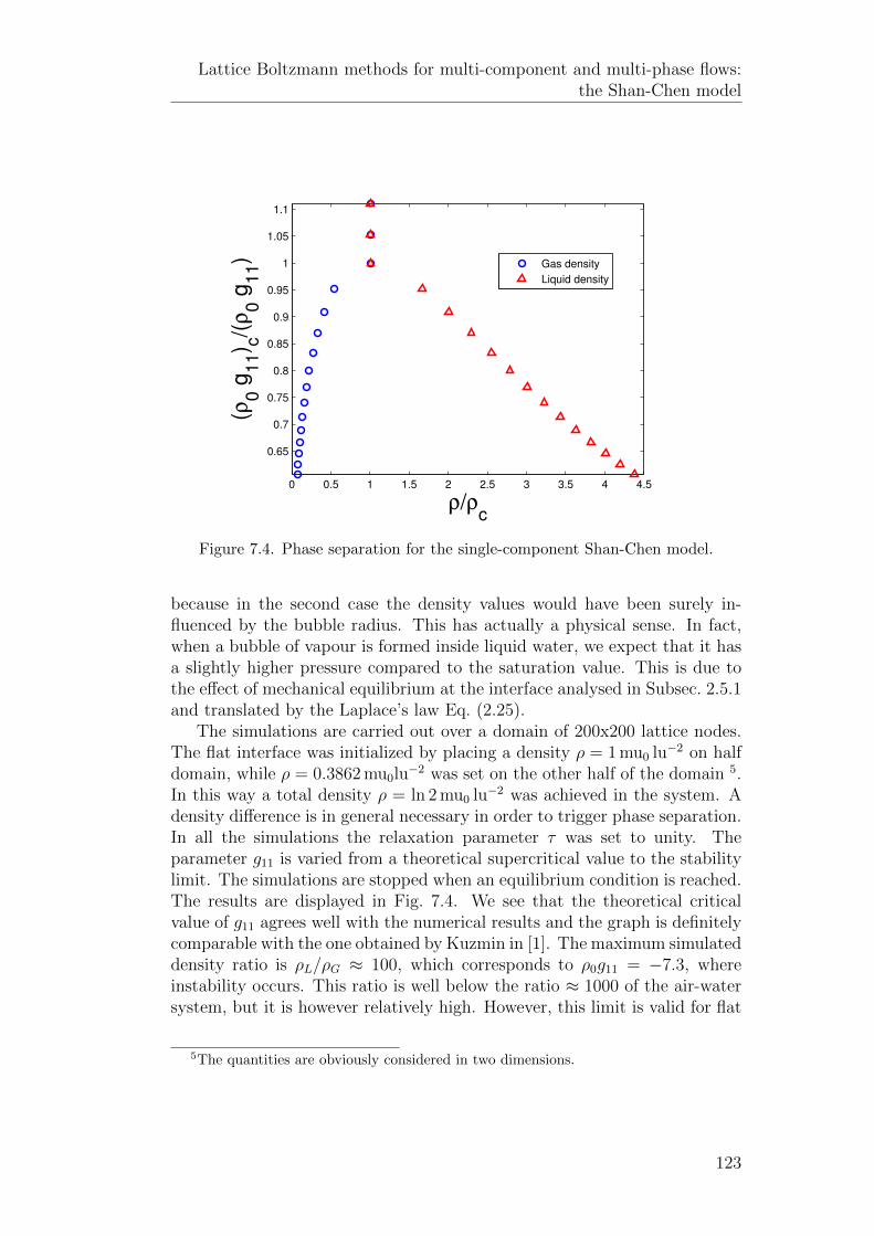
Lattice Boltzmann methods for multi-component and multi-phase flows:the Shan-Chen model
0 0.5 1 1.5 2 2.5 3 3.5 4 4.5
0.65
0.7
0.75
0.8
0.85
0.9
0.95
1
1.05
1.1
ρ/ρc
(ρ0 g
11) c
/(ρ
0 g
11)
Gas density
Liquid density
Figure 7.4. Phase separation for the single-component Shan-Chen model.
because in the second case the density values would have been surely in-fluenced by the bubble radius. This has actually a physical sense. In fact,when a bubble of vapour is formed inside liquid water, we expect that it hasa slightly higher pressure compared to the saturation value. This is due tothe effect of mechanical equilibrium at the interface analysed in Subsec. 2.5.1and translated by the Laplace’s law Eq. (2.25).
The simulations are carried out over a domain of 200x200 lattice nodes.The flat interface was initialized by placing a density ρ = 1 mu0 lu−2 on halfdomain, while ρ = 0.3862 mu0lu−2 was set on the other half of the domain 5.In this way a total density ρ = ln 2 mu0 lu−2 was achieved in the system. Adensity difference is in general necessary in order to trigger phase separation.In all the simulations the relaxation parameter τ was set to unity. Theparameter g11 is varied from a theoretical supercritical value to the stabilitylimit. The simulations are stopped when an equilibrium condition is reached.The results are displayed in Fig. 7.4. We see that the theoretical criticalvalue of g11 agrees well with the numerical results and the graph is definitelycomparable with the one obtained by Kuzmin in [1]. The maximum simulateddensity ratio is ρL/ρG ≈ 100, which corresponds to ρ0g11 = −7.3, whereinstability occurs. This ratio is well below the ratio ≈ 1000 of the air-watersystem, but it is however relatively high. However, this limit is valid for flat
5The quantities are obviously considered in two dimensions.
123

Chapter 7
interfaces, while the situation worsens for circular interfaces.In addition, an interpretation of the parameter g11 is suggested. In fact,
increasing the parameter g11 in magnitude has the same effect of decreasingthe temperature in a real system. This is due to the fact that in physicalsystem the effect of any interacting potential must be weighted by the thermalenergy kbT (see [107] for more insights). Thus, in our case we have that theeffect of the interacting potential of the Shan-Chen model is governed by theratio:
g11ψ2
kbT. (7.26)
However, kbT is a lattice constant equal to 1/3 in lattice units, and thereforethe weight is governed by the parameter g11. From Fig. 7.2 and Fig. 7.3,we can readily identify a characteristic of the Shan-Chen model, that is thepresence of a diffusive finite interface. The interface has a certain thicknessin which the density assumes intermediate values between the gas and liq-uid condition. On the contrary, the interface is usually modelled with aninfinitesimal thickness, as it is done in the derivation of the Laplace’s law. Inthis case, the interface becomes a surface of discontinuity. However, we canimagine how this is just an approximation, and in general the interface hasa certain thickness, indeed. The discontinuous modelling can be consideredvalid, when the typical thickness of the interface is much lower than the typ-ical length scale of the problem under consideration, which is true in manycases.
In the context of diffusive interface, the thermodynamic definition of thesurface tension was formulated by van der Waals during the nineteenth cen-tury and it states that [108]
σ =
∫ +∞
−∞Ψ(z) dz, (7.27)
where we are considering an infinite system with a flat interface and z iden-tifies the direction perpendicular to the interface. Ψ(z) represents the localexcess free energy density, that is the difference between the free energy withand without the interface. Eq. (7.27) is the starting point of the Cahn-Hilliard theory of surface tension [102], from which other Lattice Boltzmannmodels are originated, as it was already mentioned at the beginning of thischapter. Nevertheless, the definition of a Free-Energy for the Shan-Chenmodel is not trivial, but it has been recently achieved by Sbragaglia et al.[109], which solves the problem of lack of thermodynamical basis of the Shan-Chen model.
In Fig. 7.5 we can better appreciate the diffusive behaviour of the Shan-Chen model at interface. The density slightly goes from density values typical
124

Lattice Boltzmann methods for multi-component and multi-phase flows:the Shan-Chen model
−30 −20 −10 0 10 20 300
0.5
1
1.5
2
2.5
3
x [ lu ]
ρ [m
u 0 lu
−2
]
ρ0 g11=−4.2
ρ0 g11=−5.2
ρ0 g11=−6.2
Figure 7.5. Density as a function of x for different values of the parameter ρ0g11.The origin of the x-axis was placed approximately in the centre of the interface ineach case. The domain was taken 200x200 lattice nodes.
of the gas phase to values typical of the liquid phase. Furthermore, it isclear that the thickness of the interface decreases with the magnitude of theparameter ρ0g11. From a practical point of view, it is definitely easier todeal with thin interface thicknesses, which also represents the case of mostapplications, but, as we will see, the stability of the method is concernedwhen the interface is too thin.
As it was already stated, in this context, the Laplace’s law is no longer rig-orously valid, but it continues to represent a good approximation, especiallyat high values of ρ0g11. Thus, the usual way to obtain the surface tension isto test the Laplace’s law by running simulations with different bubble radii,keeping fixed the parameter ρ0g11. Then, by means of a linear regression(without intercept) between the pressure difference Pc and the inverse of theradius 1/R, the linear regression is obtained according to the Laplace’s lawin two dimensions Eq. (2.27). An example of this procedure is displayed inFig. 7.6.
In particular the pressure inside the bubble is evaluated at the centre,while the outside pressure is computed in one point near one of the bound-aries. It is worth noting that the radius of the disk is not an input pa-rameter. The disk is initialized with a certain radius Rin, but it is thenmodified according to the mechanical equilibrium established by the simula-tion. Thus, the final radius has to be measured, at the end of the simulation
125

Chapter 7
0.014 0.016 0.018 0.02 0.022 0.024 0.026 0.028 0.03 0.0320.8
0.9
1
1.1
1.2
1.3
1.4
1.5
1.6
1.7
1.8x 10
−3
1/R [lu−1]
Pc
[mu
0 ts
−2]
Figure 7.6. Laplace’s law verification. The parameter g11lu2 mu−10 is set to
−5 lu2 mu−10 and from the linear regression the surface tension was obtained
σ = 0.05620 mu0 lu ts−2.
and it is also not well defined, given the diffusive nature of the interface.In Fig. 7.6, the radius was assumed between the two nodes i and j, suchthat ρ(i) ≤ (ρL + ρG)/2 ≤ ρ(j). When the magnitude of ρ0g11 is relativelyhigh, the surface tension obtained by considering the minimum or maximumradius of the interface are almost equal, which of course allow us to use theaverage radius. Fig. 7.6 shows a good agreement with the Laplace’s law,which allows to obtain the surface tension of the system.
It is worth pointing out that another way of computing the surface tensionis from its mechanical definition. Considering the case of an horizontal flatdiffusive interface and an infinite system, the surface tension is given by[108]:
σ =
∫ +∞
−∞(Pyy − Pxx) dy (7.28)
where Pαα are the diagonal components of the pressure tensor. In fact, whenwe have phase separation, we can imagine how the diagonal components ofthe pressure tensor at equilibrium are not all equal as usual at the interface(and equal to the common pressure). Basically, this is the inherent cause ofthe surface tension.
Shan [110] has recently obtained an expression to compute the additionalcomponents of the pressure tensor due to the Shan-Chen interaction. Starting
126

Lattice Boltzmann methods for multi-component and multi-phase flows:the Shan-Chen model
0 50 100 150 200
0
50
100
150
200
−0.03
−0.02
−0.01
0
0.01
0.02
0.03
Figure 7.7. Difference between Pyy and Pxx ([mu0 ts−2]) for a static bubble.
from the continuum description of the intermolecular forces in which theadditional pressure tensor due to the force interaction is defined as:
∇ · ¯P I = F I , (7.29)
where here with the superscript “I” we intend that the force is an interactionforce. By applying this definition to the interaction of the Shan-Chen modeland thus considering a discrete description, the Shan-Chen pressure tensoris obtained as [110]:
¯P SC = −g11
2ψ(x)
∑i
wiψ(x+ ξi)ξiξi. (7.30)
This formula was used to compute P SCxx and P SC
yy . In Fig. 7.7 we can appre-ciate how the difference between the two diagonal components of the stresstensor assumes non zero values at the interface.
Thus, the computation of the surface tension was attempted throughEqs. (7.28) and (7.30) and compared to the results of the Laplace’s test fordifferent values of the parameter g11, keeping fixed ρ0. In particular, thetheoretical surface tension was evaluated through Eq. (7.28) for a series ofnumerical experiments with flat interface, where the integral was evaluatedalong one of the interfaces of Fig. 7.3:
σ =
∫interface
(Pyy − Pxx) dy. (7.31)
The integral is evaluated through the trapezoidal rule.
127

Chapter 7
1.15 1.2 1.25 1.3 1.35 1.4 1.45 1.5 1.55 1.60
0.02
0.04
0.06
0.08
0.1
0.12
0.14
0.16
0.18
g11
/g11,c
σ [m
u0 lu ts
−2]
σL
σTH
Figure 7.8. Laplace’s law surface tension and theoretical surface tension as afunction of g11/g11,c.
Simulations with the same parameter g11 are carried out for the staticbubble test with different radii and the simulated surface tension is obtainedthrough the Laplace’s law as described before. In these simulations ρ0 =1mu0 lu−2.
The results are displayed in Fig. 7.8. We can appreciate how both thesimulated surface tension and the theoretical surface tension increase linearlywith the parameter g11/g11,c. However, a discrepancy between the two valuesis clear, as well. In addition, Fig. 7.8 shows clearly a proportionality rela-tionship between σL and σTH . The proportionality constant was found to be1.8493 by the linear regression.
This discrepancy has been studied by Huang et al. in [85] and the reasonbehind it has been found in the inclusion of the interaction force term bythe methods of the shifting velocity of the original Shan-Chen model. Inparticular, as shown in Fig., in the original formulation the Shan-Chen modelthe surface tension, and the density ratio as well, strongly depends on therelaxation parameter τ . However, this feature seems to be shared also byother forcing schemes and by other choice of the pseudo-potential ψ [85].The dependency of the surface tension and the density ratio τ is clearlyunphysical and it is thermodynamically inconsistent. Nevertheless, as it wasargued by Kuzmin [1], this effect should be eliminated if the proper schemeproposed by Guo et al. [84] is applied to the Shan-Chen model. This agrees
128

Lattice Boltzmann methods for multi-component and multi-phase flows:the Shan-Chen model
0.01 0.02 0.03 0.04 0.05 0.06 0.07 0.08 0.090.02
0.04
0.06
0.08
0.1
0.12
0.14
0.16
0.18
σTH [mu0 lu ts−2]
σL
[mu
0 lu ts
−2]
Figure 7.9. Simulated surface tension vs. theoretical surface tension.
with the proof given in Chap. 4 and allows to identify the cause of theunphysical dependency on τ of the surface tension in the additional termsneglected in the momentum equation by other schemes, but forced to zeroby the Guo’s scheme.
Unfortunately, the Shan-Chen model is implemented in Palabos only withthe original method of the shifting velocity on the equilibrium distribution.The implementation of the Guo’s scheme would have required a considerablemodification of the code that has been avoided in this thesis and left for aneventual future work.
It is worth pointing out that the dependency of the density ratio andthe surface tension on τ are not the only inconsistencies of the Shan-Chenmodel. We have already mentioned the lack of a free-energy in the origi-nal formulation and in addition, it is shown [105], that the only form of thepseudopotential ψ which is consistent with the Maxwell’s equal area recon-struction is:
ψ(ρ) = ψ0e−ρ0/ρ. (7.32)
All these problems of the Shan-Chen model should be taken into accountwhen dealing with concrete simulations, but in general do not affect its appli-cability. For example, the simulated surface tension of the model can alwaysbe computed with the Laplace’s test without considering its discrepancyfrom the theoretical value. Anyway, from this introduction of the single-component Shan-Chen model, we can understand how a constraint of the
129

Chapter 7
model is that the density ratio and the surface tension cannot be tuned inde-pendently. Moreover, if the relaxation parameter is kept fixed, the dynamicviscosity ratio is always equal to the density ratio. A further complicationwould be to relate vary the relaxation parameter with density, in order to tunethe dynamic viscosity ratio, but even this possibility will not be analysed inwhat follows. However, we here report that Sbragaglia et al. have suggestedthat the surface tension and the density ratio can be tuned independentlyby considering also the interaction with the second layer of neighbours [32],giving rise to the so-called multi-range model.
Let us now focus on another interesting feature of the Shan-Chen modelfor single-component fluid that is the behaviour nearby the critical point. Itis known that different critical phenomena such as gas-liquid transition andferromagnetic transition shares similar critical behaviour as a function of theparameter that governs the transition, which is typically temperature. Incritical transitions, an order parameter can be identified, which takes intoaccount the phase separation. For example, in gas-liquid transition, therole of the order parameter is accomplished by the difference between liquidand gas density, while in ferromagnetic transition it is carried out by themagnetization. The order parameter goes to zero at the critical point and itshows a power law behaviour as a function of the parameter governing thetransition:
Λ ∼ θβΛ , (7.33)
where here we are denoting by Λ a certain order parameter and by θ the asso-ciated transition parameter. Surprisingly enough, order parameters from dif-ferent phenomena not only behaves as a power law, but seem to share also thesame exponent βΛ. The critical behaviour of the Shan-Chen transition hasbeen investigated considering the order parameter ΛSC = (ρL − ρG)/ρL andas transition parameter θSC = (ρ0g11)c[1/(ρ0g11)c − 1/(ρ0g11)]. In Fig. 7.10,we are able to see how the power law behaviour is perfectly recovered bythe Shan-Chen model. Furthermore, the exponent of the transition is foundβSC ≈ 0.5. This definitely puts the Shan-Chen model in the framework ofmean field theory. In fact, the mean-field theories of van der Waals and Curie-Weiss for gas-liquid transition and ferromagnetic transition respectively, pre-dict both a critical exponent equal to 1/2 [107]. For more insights on thecritical behaviour of the Shan-Chen model see [111].
As a final issue for the single-component Shan-Chen model we deal withthe effective verification of the static bubble test. As we have previouslymentioned we expect the velocity field to be everywhere zero and the bubbleto remain at the centre of the domain, where it is initially placed with asymmetrical disk shape in two dimensions. Obviously, the radius of thebubble generally varies from the initial value, unless we have correctly guessed
130

Lattice Boltzmann methods for multi-component and multi-phase flows:the Shan-Chen model
−5.5 −5 −4.5 −4 −3.5 −3−0.8
−0.6
−0.4
−0.2
0
0.2
0.4
0.6
ln(ρ0 g
11)c[1/(ρ
0 g
11)c−1/(ρ
0 g
11)]
ln[(
ρL−
ρG
)/ρ
c]
Figure 7.10. Order parameter as a function of the transition parameter for thesingle-component Shan-Chen model.
the equilibrium gas and liquid density at the beginning of the simulations,which is of course a very unlikely event.
Fig. 7.11(a) shows the velocity norm field scaled by cs = 1/√
3, thatis the Mach number. The velocity is basically everywhere zero, except atthe interface where we have high velocities. These unphysical velocities areusually called spurious currents and are definitely one of the main concern ofthe Shan-Chen model. It should be noted that the structure of the velocityfield resembles that of the underlying lattice. The velocity vectors shown inFig. 7.11(b) allow us to identify the presence of circulating flows through theinterface. In Fig. 7.12, we can grasp how the spurious velocities are normal tothe interface, when the x-axis or the y-axis are perpendicular to the interface6. The spurious currents are not only a feature of the Shan-Chen model, butthey are also present in multi-phase schemes based on free-energy.
The spurious currents not only complicates the analysis of the result ofthe simulations, but are also the cause of the instability of the simulationswhen the parameter ρ0g11 increases in magnitude. In fact, the spuriousvelocities are connected to the density gradient at interface and thus whenρ0g11 becomes more negative 7, leading to higher density ratios and lower
6Actually, we are able to notice it also in Fig. 7.11(b), if we look carefully at it7In this case we are obviously considering the pseudopotential ψ = 1 − e−ρ/ρ0 , but
131

Chapter 7
(a) Mach number field u/cs.
(b) Velocity vectors.
Figure 7.11. Spurious velocities for the static bubble test.
132

Lattice Boltzmann methods for multi-component and multi-phase flows:the Shan-Chen model
(a) Ux/cs (b) Uy/cs
Figure 7.12. Scaled velocity components.
interface thickness, we expect the spurious currents to increase in magnitudeleading to instability [1], whose main origin lays in the expansion of theMaxwellian distribution function for low Mach number Eq. (3.53). In fact,this is the reason of the limited density ratios of the Shan-Chen model.
It is established in literature that the origin of the spurious currents isthe not sufficient isotropy of the interaction force term and are present onlywhen the interface has a certain curvature [112]. Great effort has been madein recent years in order to reduce the spurious currents. The interpretationof the spurious currents given by Shan in [112] has been further investigatedin [32] by Sbragaglia et al., which has proposed the already mentioned multi-range potential model, which increases the isotropy of the force term andallows to reduce the spurious currents. However, another method of dealingwith the spurious currents has been proposed by Yuan & Schaefer in [5] andconsists in incorporating different equation of state (EOS) in the Shan-Chenmodel. We will come back to this approach in the following section, since ithas also other interesting feature.
After the analysis of the static test for the single-component Shan-Chenmodel, we will now treat the multi-component Shan-Chen model. Since themain features of the Shan-Chen model have been already highlighted bythe single-component case, and are basically shared by the multi-componentcase, we will just briefly tackle the issue of the multi-component Shan-Chenmodel, focusing on its immiscible behaviour.
Thus, let us consider a multi-component system where only the interac-tion between the two components is considered, which means g11 = g22 = 0.
analogous considerations can be made for different choices of ψ.
133

Chapter 7
0 0.5 1 1.5 2 2.5 3 3.5 4 4.50
0.1
0.2
0.3
0.4
0.5
0.6
0.7
0.8
0.9
1
ρ0 g
12
x1
Inside the bubble
Outside the bubble
(a) Mass fraction of component 1
0 0.5 1 1.5 2 2.5 3 3.5 4 4.50
0.1
0.2
0.3
0.4
0.5
0.6
0.7
0.8
0.9
1
x2
ρ0 g
12
Inside the bubble
Outside the bubble
(b) Mass fraction of component 2
Figure 7.13. Immiscible behaviour of the multi-component Shan-Chen model.
134

Lattice Boltzmann methods for multi-component and multi-phase flows:the Shan-Chen model
According to Eq.(7.22), the equation of state for the system becomes:
p =ρ1 + ρ2
3+
1
3g12ρ1ρ2, (7.34)
where we are considering lattice units and we have set the multi-componentpseudopotential ψσ equal to ρσ for both components as usual in literatureand how it is implemented in Palabos.
The immiscible behaviour of the multi-component case is investigated inthe case of a static bubble. In fact in this case, the flat interface and thestatic bubble do not differ too much, since we are actually interested in themass fractions of each component. In this case, the results are scaled by thetotal density of the system which has now the role of ρ0 and fixes the massscale mu0 [106]. In addition, the critical value of the parameter ρ0g12 is equalto unity [106].
Thus, in order to initialize the simulation, a disk is placed at the centreof a 126x126 lattice nodes. The radius of the disk is equal to 50 lu andthe density of component 1 and 2 are set respectively to ρ1 = 1 mu0 lu−2
and ρ2 = 0 mu0 lu−2. On the contrary, outside the disk the densities areset ρ1 = 0 mu0 lu−2, ρ2 = 1 mu0 lu−2. In this way the total mass fractionsare approximately equal to 1/2, i.e., the critical mass fractions. By varyingg12 we obtain different mass fractions as usual. In all the simulations therelaxation parameter τ is set to 1. When the mass fractions of the fluidsbecome stationary the simulation is stopped as usual. The results are shownin Fig. 7.13.
We are able to see that the numerical critical value of the parameterρ0g12 matches the theoretical findings. For ρ0g12 greater than the criticalvalue (ρ0g12)crit = 1, the system separates itself in two phases with differentmass fractions. The separation curve is now strictly symmetric.
It should be noted that, in this case, it is possible to tune the kinematicviscosity ratio taking different values of τ for the two components. However,only viscosity ratios close to unity are allowed due to instability.
Analogously to the single-component case, the computation of the sur-face tension can be made by means of the Laplace’s law and the surfacetension increases with ρ0g12. Nevertheless, a serious limitation of the multi-component Shan-Chen model is that the density ratios are always very closeto 1. In general, it is very difficult to tell whether the higher density will beinside the disk or outside it. A further complication would be to include alsothe single-component interactions in the multi-component model, which leadto the general equation of state reported in Eq. (7.22).
135

Chapter 7
7.3 Incorporating EOS
In Sec. 7.2 we have started to become familiar with the Shan-Chen modelin its original formulation. The main criticalities have also been highlightedand they can be summarized in:
• spurious currents;
• coupling between density ratio and surface tension;
• unphysical dependency of the surface tension on the relaxation param-eter.
We have also seen that recent the literature on the Shan-Chen model hasfocused on the solution of these problems. Basically two approaches havebeen proposed to deal with these issues:
1. the introduction of a multi-range pseudopotential (Sbragaglia et. al[32]);
2. the incorporation of physical Equation of State (EOS) (Yuan & Schae-fer [5]).
In particular, the multi-range potential method, in which the interaction isextended to the next layers of neighbours, seems to reduce all the above-mentioned problems, but the price to be paid is an higher computationalcost. On the other hand, the usage of physical EOS seems to allow a greatreduction of the spurious currents, achieving much higher density ratio whencompared to the original formulation of the Shan-Chen pseudopotential withbasically the same computational cost. Furthermore, dealing with commonEOS is definitely easier and leads to more physical situations.
It is worth pointing out that the idea behind the multi-range potentialis supported in [32] by the theoretical interpretation of the nature of thespurious currents, that is the insufficient isotropy of the interaction forceterm. The multi-range potential implies an improvement of isotropy andthus, a reduction of spurious currents. On the contrary, the introduction ofa physical EOS on the Shan-Chen model seems to yield improvements, buttheoretical basis lack and they are limited to the more physical behaviour ofthe system.
Neither the method of the multi-range potential, nor the introduction ofan EOS is implemented in the current version of the Palabos library. Thus,in order to test one of the two methods a bit of coding was needed. Since theincorporation of the EOS was considered more easily feasible, this approachhas been chosen. The implementation of the multi-range potential seems
136

Lattice Boltzmann methods for multi-component and multi-phase flows:the Shan-Chen model
also feasible, even though it requires a greater modification of the sourcecode, and for this reason it is left as an eventual future work. Thus, we nowintroduce the main ideas behind the method of the incorporation of physicalEOS.
Let us begin by considering the single-component equation of state ofthe Shan-Chen model Eq. (7.23). Now, the idea is very simple, indeed.This equation can be recast in order to obtain an explicit formula for theinteraction potential:
ψ =
√6(p− c2
sρ)
g11
. (7.35)
This allows an ad hoc construction of the pseudopotential in order to matchthe desired EOS. In fact, considering for example the van der Waals equationof state:
p =ρRT
1− bρ− aρ2, (7.36)
we can compute the pressure as a function of ρ in each point of the latticeand then inserting it into Eq. (7.35) to obtain the pseudopotential in thatpoint. Afterwards, the pseudopotentials can be used in Eq. (7.12) to obtainthe interaction force as usual.
The first new feature of this approach is the direct introduction of atemperature in the system. In the original scheme, we have seen that theconcept of temperature was connected to the parameter g11. An increaseof g11 in magnitude meant a decrease of temperature. In this case, thetemperature is incorporated into the pseudopotential, carrying out the samequalitative role of g11. In addition, it is worth noticing that the role of theparameter g11 in this scheme is only to guarantee that the argument of thesquare root remains positive. Since, g11 needs to be negative to ensure phaseseparation in the original SC model, we expect the same behaviour in thiscase.
In Yuan & Schaefer’s [5] paper, the two EOS which gave the best per-formances were the Carnahan-Starling (CS) and the Peng-Robinson (PR).Hence, we will now focus on these equations of state.
The Carnahan-Starling EOS [43] is basically the evolution of the van derWaals EOS:
p = ρRT1 + bρ/4 + (bρ/4)2 − (bρ/4)3
(1− bρ/4)3− aρ2, (7.37)
where a and b are the two parameters of the equation. The parameters ofthe simulations are of course connected to the critical temperature Tc andpressure pc:
a = 0.4963T 2c R
2
pc, b = 0.18727
RTcpc
, (7.38)
137

Chapter 7
0 0.5 1 1.5 2 2.5 3 3.5
0.6
0.7
0.8
0.9
1
1.1T
/Tc
ρ/ρc
Gas density
Liquid density
Figure 7.14. Phase separation for the Carnahan-Starling EOS.
from which we can obtain the critical compressibility factor Zc = pc/(ρcRTc) =0.35930763 [113] and consequently the critical density ρc. We will use thesame parameter chosen in [5], that isR = 1 [lu2 ts−2 K−1
0 ], a = 1 [mu−10 lu3 ts−2]
and b = 4 [lu2 mu−10 ] 8. These choices fixes a mass scale mu0 and an absolute
temperature scale K0, when converting to physical units. However, in whatfollows we will always report the result in a reduced quantity system for thesake of clarity. The reduced temperature, pressure and density are obviouslydefined:
T =T
Tc, p =
p
pc, ρ =
ρ
ρc. (7.39)
In order to explore the immiscible behaviour of the CS, simulations werecarried out for the case of a flat interface, similarly to what has been donefor the original SC model in Sec. 7.2. The domain size was 200x200 latticenodes. A small density difference is initialized in the two halves of the domainand the total density of the system is kept equal to the critical one in all thesimulations. In all the simulations the relaxation parameter τ was set tounity. In this case the temperature is varied in place of the parameter g11
from supercritical to subcritical values. The results are shown in Fig. 7.14.The minimum value of the reduced temperature achieved was T/Tc =
0.5408, which corresponds to a density ratio ρL/ρG = 53 827. This result
8Of course, the units are for the 2D case.
138

Lattice Boltzmann methods for multi-component and multi-phase flows:the Shan-Chen model
0 0.5 1 1.5 2 2.5 30.75
0.8
0.85
0.9
0.95
1
1.05
1.1
T/T
c
ρ/ρc
Gas density
Liquid density
Figure 7.15. Phase separation for the Peng-Robinson EOS.
is valid for flat interfaces where the spurious currents are lower than thestatic drop/bubble case. However, it is definitely much higher than the valueρL/ρG ≈ 100, reported in Sec. 7.2 for the original SC pseudopotential.
The Peng-Robinson EOS belongs to the family of cubic equations of state[42]. Its formulation is:
p =ρRT
1− bρ− aα(T )ρ2
1 + 2bρ− b2ρ2,
α(T ) = [1 + (0.37464 + 1.54226ω − 0.26992ω2)(1−√T/Tc)]
2.
(7.40)
The parameter ω is called acentric factor and is dependent on the speciesunder consideration. In case of water it is equal to 0.344. The parameters aand b of the EOS are connected to the critical temperature and pressure bythe following relationships:
a = 0.45724R2T 2
c
pc, b = 0.0778
RTcpc
. (7.41)
This yields a critical compressibility factor Zc = 0.307 [42]. Similarly tothe case of CS equation we set the same parameter a and b of [5]: R =1 [lu2 ts−2 K−1
0 ], a = 2/49 [mu−10 lu3 ts−2] and b = 2/21 [lu2 mu−1
0 ].In Fig.7.15, we can see the phase diagram for the PR EOS. The acentric
factor in this case is ω = 0.344, which is the acentric factor of water. In this
139

Chapter 7
Rin[lu] ρinL /ρc ρinG /ρc (ρ0g11)c/(ρ0g11) T/Tc umax/cs
SC 30 2.913 0.2040 0.7825 / 0.2653
CS 30 2.213 0.1548 / 0.8 0.1921
PR 30 2.307 0.1616 / 0.88418 0.1428
Table 7.1. Numerical parameters and results of the fixed density ratio test. Here,SC denotes the original Shan-Chen model, CS the Carnahan-Starling EOS andPR the Peng-Robinson EOS.
case, the maximum density ratio achieved in this case is ρL/ρG = 767, whichis related to T/Tc = 0.75. This value is lower than the maximum densityratio of the CS EOS. This is a first evidence of an initialization problem,which affects the Shan-Chen model.
So far, we have only dealt with flat interfaces, but in reality we are inter-ested in curved interfaces. The Shan-Chen model for curved interfaces yieldsalways higher spurious currents than the flat interface test. Thus, in orderto compare the Carnahan-Starling EOS, the Peng-Robinson and the originalShan-Chen pseudopotential we need to consider the static circular test. Inparticular, two tests will be conducted in order to evaluate which is the bestmodel between the three alternatives. Considering always a fully periodicdomain of 200x200 lattice units, a circular interface of radius 30 lattice unitsis initialized, with the liquid phase inside it. Reasonable values for the liquidand the gas phase can be obtained from the simulations for flat interfaces.Accordingly, at the interface we have a jump discontinuity. In the first test,the parameters governing the phase separation, that is ρ0g11 for the originalSC model, and T/Tc for the CS and PR equations of state, are tuned inorder to achieve the same density ratio. Then, the static drop simulationsare carried out for the three models and the results compared in terms ofmaximum magnitude of the spurious currents. Each simulation has been runfor 50 000 iterations. It is worth noticing that the final radius will never beexactly the same for the three phases due to compressibility. The densityratio was fixed to ≈ 14.28, which is the equilibrium density ratio of the CSequation when T/Tc = 0.8. The parameters of the other two equations arethen adjusted to obtain this ratio. The acentric factor of the Peng-Robinsonis fixed and equal to that of water ω = 0.344.
We can see the velocity field of the different models in Fig. 7.16. The inputparameters and the numerical result in terms of maximum magnitude of thespurious currents are shown in Table 7.1. Both the CS and PR equationsof state show a lower maximum velocity compared to the original SC, eventhough they remain of the same order of magnitude. In particular, the PR isthe EOS which performs the best result, decreasing the maximum velocity of
140

Lattice Boltzmann methods for multi-component and multi-phase flows:the Shan-Chen model
(a) u/cs for the original SC.
,(b) u/cs for the CS EOS.
(c) u/cs for the PR EOS.
Figure 7.16. u/cs field for the different pseudopotentials.
141

Chapter 7
ρinL /ρc ρinG /ρc ρL/ρG (ρ0g11)c/(ρ0g11) T/Tc umax/cs Reason
SC 4.194 0.08195 47.46 0.625 / 0.5413 Drop movement
CS 2.621 0.06410 37.49 / 0.73 0.2694 Initial instability
PR 2.622 0.06472 37.37 / 0.82 0.2289 Initial instability
Table 7.2. Numerical parameters and results of the limiting density ratio test.Here, SC denotes the original Shan-Chen model, CS the Carnahan-Starling EOSand PR the Peng-Robinson EOS.
the original SC by almost a factor 2. From, Fig. 7.16, we can grasp the reasonof this reduction in the higher interface thickness of the PR EOS. The densitygradients of the PR EOS are smoother than the others, leading to lowerspurious currents. On the other hand, as we know, high interface thicknessesrather complicate the analysis of the result and the application to physicalsystems, in which the interface is usually negligible. It is worth pointing outthat, here we witness higher spurious currents than those reported in [5],where a similar test was conducted in three dimensions.
In the second test, the density ratios are pushed over their limits for thethree models, until instability occurs. In particular, this instability may benumerical or physical. In fact, it has been witnessed that even though thesimulations where numerically stable, at high density ratio the simulationsshowed an odd behaviour. For instance, phenomenon like movement of thedrop towards a certain direction or loss of sphericity have been observed,which took place even after many time steps. Since, this behaviour has nophysical sense, and the model cannot be applied in this regime for practicalpurposes, it was decided to reject these results.
The size of the domain remains the same of the previous test, as wellas the relaxation parameter and the number of iterations. In order to carryout a “fair” test, the initial gas and liquid densities are taken in each casefrom the relative flat interface test. Thus, a sharp initialization has beenused, where the interface is discontinuous. The reason of this clarificationwill become understandable in what follows. The initial radius in each testis rin = 30 lu. Little differences have been observed between the final andinitial radius. The limiting results of this test are summarized in Table 7.2.In particular, in Table 7.2 all the results are physically and numerically. Thecause of instability at higher density ratio is also reported, as well as theinitial liquid and gas densities.
From Table 7.2, we see that in this test, the highest density ratio hasbeen obtained with the original Shan-Chen model. In particular, we noticethat both the CS and PR EOS show lower spurious velocities with respect tothe original SC model, but suffer a problem of initialization, probably due to
142

Lattice Boltzmann methods for multi-component and multi-phase flows:the Shan-Chen model
ρinL /ρc ρinG /ρc ρL/ρG T/Tc umax/cs Reason
CS 2.767 0.02073 146.36 0.65 0.3731 Initial instability
PR 2.883 0.01556 185.29 0.75 0.3343 Initial instability
Table 7.3. Numerical parameters and results for the CS and PR EOS when theyare initialized with a diffusive interface. The interface thickness in this case is of10 lu. In the interface the density varies linearly from ρL to ρG.
ρinL /ρc ρinG /ρc ρL/ρG T/Tc umax/cs
CS 3.142 0.1139 518.6 0.6 0.4491
Table 7.4. Example of density ratio achieved with the CS EOS.
the high spurious velocities at the beginning of the simulation. We see also,that this happens for the CS and the PR for a similar density ratio. Thisinitialization issue might be very annoying in practice, but it may be worththe effort, since it allows to achieve higher density ratios. In fact, by meansof a smoother initialization, in which also the diffusive interface is initialized,higher density ratios can be obtained. We can see in Table 7.3, that theCS and and PR allows to simulate higher density ratios. In these cases nophysical instability have been observed. In addition, the values here reportedare the respective limiting cases, when the interface thickness is initializedwith 10 lu.
Even higher density ratios can be achieved by not matching the initialvalues of the flat interface test and initializing with intermediate densities. Inthis case, the main shortcoming is that the final radius will very inevitablyfrom the initial one. As an example, we report the result that has beenobtained for the CS EOS, which has proved to be more flexible than the PREOS from this point of view, in Table 7.4, which should not be intended asa limiting value.
From this simple tests, we conclude that the EOS approach in the Shan-Chen model allows to reduce the spurious velocities given a fixed densityratio and to achieve higher density ratios, compared to those of the originalShan-Chen model. However, if we want to use EOS at high density ratioswe have to cope with the initialization issue.
In Sec. 7.5, we will see that there is also another issue, which is for nowhidden in the use of EOS.
143

Chapter 7
(a) u/cs for the original SC.
,(b) u/cs for the CS EOS.
(c) u/cs for the PR EOS.
Figure 7.17. u/cs field for the different pseudopotentials at the stability limit(Table7.2 ).
144

Lattice Boltzmann methods for multi-component and multi-phase flows:the Shan-Chen model
(a) Total wet: ρW /ρc = 2.170. (b) Wet: ρW /ρc = 1.4738.
(c) Non-wet: ρW /ρc = 0.3684. (d) Total non-wet: ρW /ρc =0.1936.
Figure 7.18. Different wetting conditions for the liquid phase.
7.4 Determination of the contact angle
So far, we have only seen how the Shan-Chen model allows to take into ac-count the interparticle forces by means of a fictitious pseudopotential. How-ever, when dealing with flows in porous media, we need also to incorporatethe interaction of the two phases with the surface in order to obtain differentcontact angles. Even this task can be surprisingly carried out by means of afictitious additional interaction with the solid boundaries. The form of theinteraction is the following for the single component case [114]
F ad = −g11ψ(ρ(x))∑i
wiψ(ρW )s(x+ ξi)ξi, (7.42)
where s is a function that is equal to 1 if the node x + ξi is a solid node (aBounce-Back node for example) and 0 if it is a fluid node. The density ρW isa fictitious density attributed to the boundary node. By changing its valueit is possible to achieve different contact angles and wetting conditions. Inparticular, we expect that values of ρW close to the gas/liquid density wouldmean that the gas/liquid is the wetting phase. Even in this case the contactangle can be evaluated by means of a simple test.
In Fig. 7.18, we can see how different wetting conditions can be achievedby tuning the wall density ρW . In particular, Fig. 7.18 has been obtained forthe PR EOS with T/Tc = 0.9. In this condition, the liquid and gas densityare respectively ρL/ρc = 2.170 and ρG/ρc = 0.1936. In fact, when ρW/ρcequals these values, we obtain total wetting/non-wetting conditions.
It is worth noticing that by changing the value of ρw in the domain wecan easily achieve also space dependent wetting conditions. In particular,this situation may occur in oil reservoir in which there might be water-wetzones, as well as oil-wet zones.
145

Chapter 7
An important observation is that the contact angle can definitely be ad-justed at will with the Shan-Chen model to match that of real physicalsystems.
7.5 Relative permeability in a 2D co-current
channel
In Sec. 7.3, we have seen how the incorporation of physical EOS, such as thethe Peng-Robinson or the Carnahan-Starling, in the Shan-Chen pseudopo-tential, allows to achieve higher density ratio, reducing the magnitude of thespurious currents. In the fixed density ratio test, the Peng-Robinson EOSwas the one that produced the lowest spurious currents. For this reason, wewill consider the PR form of the SC pseudopotential at the beginning of thissection.
The aim of this section is to validate the Shan-Chen model in the simplecase of a two-dimensional co-current channel, already described in Sec. 2.5.3.A similar validation has been carried out in [37, 49, 115, 50] for the respectiveLBM models.
Indeed, in the context of porous media, we are interested in achievinghigh density ratios, in order to obtain a wider range of dynamic viscosityratios (M). In fact, in Sec. 2.5.3 we have pointed out the influence of theparameter M in the relative permeability curves. The magnitude of thiseffect is particularly strong in the 2D co-current channel as we can see fromEqs-(2.35).
We have seen also that in the Shan-Chen model the relaxation parameterτ is in general fixed for both phases, and consequently the kinematic viscosityratio is fixed and equal to 1. This obviously means that the dynamic viscosityratio M is equal to the density ratio:
M =µnwµw
=ρnwρw
. (7.43)
Being aware of this constraint, let us begin our validation by considering thecase of a 2D co-current flow, where the wetting phase is the one with thehighest dynamic viscosity, that is the liquid phase. The domain is similarto that displayed in Fig. 2.6 and it is composed of 201x102 lattice nodes.The Peng-Robinson EOS has been used with the same parameters reportedin Sec. 7.3. The reduced temperature is equal to T/Tc = 0.9, and yields adensity ratio ρL/ρG = 11.21. According to the definition given in Eq. (7.43),the dynamic viscosity ratio is M = 0.08921. The fictitious density at walls isequal to ρw = ρL, where Bounce-Back boundary conditions are applied. The
146

Lattice Boltzmann methods for multi-component and multi-phase flows:the Shan-Chen model
0 0.2 0.4 0.6 0.8 10
0.2
0.4
0.6
0.8
1
1.2
1.4
Sw
kr,
w,
kr,
nw
Wetting (LBM PR)
Non−wetting (LBM PR)
Wetting (Analytical)
Non−wetting (Analytical)
Figure 7.19. Comparison between the analytical and numerical relative permeabil-ities of the PR EOS. M = 0.08921: the liquid is the wetting phase.
relaxation parameter is always equal to 19. The numerical experiment hasbeen carried similarly to [37, 49, 115, 50]. Periodic boundary conditions areapplied in the x-direction. The role of the pressure gradient in Eqs. (2.33) and(2.34) is carried out by a constant force per unit of area F 10, applied to bothfluids, and obviously directed in the x-direction 11. In all the simulations F =10−8mu0lu−1ts−2. The liquid and the gas densities are initialized taking thecorresponding results of the flat interface test. The position of the interfaceis assumed between the two nodes i and j such that ρ(i) ≤ (ρL + ρG)/2 ≤ρ(j). Of course, the inherent diffusive nature of the interface may generateambiguities in this definition. The relative permeabilities of the wettingand the non-wetting phases can be simply obtained as the ratio betweenthe Darcy’s velocity of the present experiment, and the Darcy’s velocity incase the channel is occupied either by only the wetting phase or only by thenon-wetting phase.
The results are shown in Fig. 7.19. We can see a clear tendency ofthe LBM simulations to underestimate the relative permeability of the non-wetting phase, while the agreement seems better achieved for the wetting
9This specification will be omitted in what follows10It would be per unit of volume in 3D.11From now on we will call it F being aware of its direction.
147

Chapter 7
0 20 40 60 80 1000
0.2
0.4
0.6
0.8
1
y [lu]
ux/u
max
Analytical
LBM PR
Figure 7.20. Comparison between the analytical and numerical velocity profilesfor the PR EOS. Sw ≈ 0.4 and M = 0.08921: the liquid is the wetting phase.
phase, except for the case Sw = 0.9. This observation is further supported byFig. 7.20, where the predicted velocity of the non-wetting phase is definitelylower than the analytical one. The reason of this behaviour has been found inthe diffusive nature of the interface obtained with Shan-Chen model. In fact,we can expect the velocity gradients of a diffusive interface to be smootherthan those of a sharp interface. This effects seems to influence mostly thethe non-wetting phase in this case. It seems also that there is a slight loss ofsymmetry. A similar behaviour has been obtained in [37], but not supportedby explanations.
Nevertheless, we have previously observed in Sec. 7.3, and in particularin the analysis of Fig. 7.16, that the PR EOS was certainly the one thatproduces the greatest interface thicknesses given a fixed density ratio. Fromthis observation, we are lead to expect that the best results should be ob-tained with the original SC, which was the model with the lowest interfacethickness, while intermediate results are expected from the CS EOS.
For this reason, also the CS and the original SC model (which we willsimply denote by SC) have been tested by matching the same dynamic vis-cosity ratio. In particular this corresponds to T/Tc = 0.8335 for the CS EOS,and (ρ0g11)/(ρ0g11)c = 1.230 for the SC model.
The comparison between the three models and the analytical solution isshown in Fig. 7.21. As it was foretold, the SC model shows the best agreement
148

Lattice Boltzmann methods for multi-component and multi-phase flows:the Shan-Chen model
0 0.2 0.4 0.6 0.8 10
0.2
0.4
0.6
0.8
1
1.2
1.4
Sw
kr,
w, k
r,nw
Wetting (Analytical)
Non−wetting (Analytical)
Wetting (LBM PR)
Non−wetting (LBM PR)
Wetting (LBM CS)
Non−wetting (LBM CS)
Wetting (LBM SC)
Non−wetting (LBM SC)
Figure 7.21. Comparison between the analytical and numerical relative permeabil-ities of the PR, CS and SC. M = 0.08921: the liquid is the wetting phase.
with the analytical solution due to its thin interface, followed by the CS andthe PR EOS. In addition, also the comparison between the velocity profilesis reported in Fig.7.22, where the velocities are made dimensionless usingthe maximum analytical velocity, which in turn shows the better agreementof the original SC. Here we are able to appreciate the smoother velocitygradients of the PR and CS compared to the original SC.
For the sake of completeness, we considered also the case with M > 1,in which the liquid is the non-wetting case and the gas the wetting phase.The parameters are basically the same as before, with the exception that thefictitious density at wall is now equal to ρG. We can see the results in termsof relative permeabilities in Fig. 7.23. Even in this case, the tendency tounderestimate the relative permeability of the non-wetting phase is clear. Inturn, the original SC model shows better results than the CS and PR EOS.In Fig. 7.24, we can see the comparison with the analytical result for thecase Sw ≈ 0.4. Basically, the same phenomenon as before can be observedregarding the velocity gradients at the interface. However, we can also see astrange behaviour of the SC model at the beginning of the interface, wherethe velocity seems to decrease. This is also slightly shown by the CS model,while the PR model does not show this effect. An interpretation of this effectmight be the influence of the spurious velocity along the y-direction, whichmay cause a first inertia effect. This also explains why this behaviour is more
149

Chapter 7
0 20 40 60 80 1000
0.2
0.4
0.6
0.8
1
y [lu]
ux/u
max
Analytical
LBM PR
LBM CS
LBM SC
Figure 7.22. Comparison between the analytical and numerical velocities of thePR, CS and SC. The velocity profiles are scaled with the maximum analyticalvelocity, in order to allow a comparison.Sw ≈ 0.4 and M = 0.08921: the liquid isthe wetting phase.
0 0.1 0.2 0.3 0.4 0.5 0.6 0.7 0.8 0.9 10
1
2
3
4
5
6
7
Sw
kr,
w, k
r,n
w
Wetting (Analytical)
Non−wetting (Analytical)
Wetting (LBM PR)
Non−wetting (LBM PR)
Wetting (LBM CS)
Non−wetting (LBM CS)
Wetting (LBM SC)
Non−wetting (LBM SC)
Figure 7.23. Comparison between the analytical and numerical relative permeabil-ities of the PR, CS and SC. M = 11.21: the gas is the wetting phase.
150

Lattice Boltzmann methods for multi-component and multi-phase flows:the Shan-Chen model
0 20 40 60 80 1000
0.2
0.4
0.6
0.8
1
Sw
kr,
w, k
r,nw
Analytical
LBM PR
LBM CS
LBM SC
Figure 7.24. Comparison between the analytical and numerical velocities of thePR, CS and SC. The velocity profiles are scaled with the maximum analyticalvelocity, in order to allow a comparison.Sw ≈ 0.4 and M = 11.21: the gas is thewetting phase
pronounced for the original SC model.Finally, Fig.7.25 shows how the CS EOS can be used to simulate flows
with higher density ratios. In this case, ρL/ρG = 65.83, and since the liq-uid is the wetting phase M = 1/65.83 = 0.01519. This ratios begin to beunattainable by the original Shan-Chen model. Basically, the analysis is thesame as before. Anyway, we expect that at higher density ratios the CS EOSwould take advantage of the reduction of the interface thickness and thus,the agreement with the analytical solution should be improved. Indeed, wehave also to take into account that the velocity gradients become sharper.Consequently, the presence of a diffusive interface weights more in this prob-lem and we do not witness a definite improvement of the agreement with theanalytical solution.
From this test case, we conclude that if the density ratios are relativelylow the original Shan-Chen model should be preferred over the EOS models,while the CS and PR EOS should be employed to explore higher densityratios. However, it is worth pointing out that the 2D co-current channel isa particularly favourable test case, since we are dealing with flat interfacesand the spurious velocities are consequently directed in the y-direction. Thesituation may change when considering curved interfaces, in which case the
151

Chapter 7
0 20 40 60 80 1000
0.2
0.4
0.6
0.8
1
y [lu]
ux/u
max
Analytical
LBM CS
Figure 7.25. Comparison between the analytical and numerical velocity profilesfor the CS EOS. Sw ≈ 0.4 and M = 0.01519: the liquid is the wetting phase.
models should be subjected to a further validation, that has not been carriedout neither in this thesis, nor in other similar works [37, 49, 115, 50]. Wehere report that some validation has been achieved for the rising bubble testin [116], while a comparison with experimental data has been carried out in[38], although both with limited density ratios.
152

Chapter 8
Conclusions
In this thesis, the Lattice Boltzmann methods for fluid dynamics have beendiscussed theoretically and practically, with particular attention to flows inporous media. We have reported how the Lattice Boltzmann equation canbe obtained as a proper discretization of the Boltzmann equation, whichdefinitely set the methods in the framework of Statistical Mechanics. Theconnection between the Navier-Stokes equations have been shown by meansof the Chapman-Enskog expansion, where we have also identified the methodproposed by Guo et al. [84], as the correct way of including the forcing termin the LBE.
All the numerical simulations in this thesis have been carried out bymeans of the Palabos library. In addition, all the simulations were relatedto two-dimensional problems. The numerical study of single-phase flows hasdefinitely shown that the LBMs are a valid tool in the context of porousmedia. In particular, in this context the easy handling of complex geome-tries by means of the Bounce-Back boundary conditions is a key element inthe success of the methods. Moreover, the TRT model should be preferredover the BGK model and other versions of the MRT model in porous me-dia applications, because it allows to annul the unphysical dependency ofthe permeability on the viscosity. A validation has been carried out for theHagen-Poiseuille flow and the flow over a hexagonal array of disks showinggood agreement with the analytical or semi-analytical formulas available. Inaddition, the LBM with the TRT collision term has been used to verify theCarman-Kozeny model to predict the permeability, in a random array ofdisks. The simulations have shown a general validity of the model, especiallyat moderate porosities.
The study of two-phase flows has been introduced considering the Shan-Chen model, which is the first multi-phase model proposed in the LBMliterature. The main characteristics of the original model have been discussedand shown using the numerical simulations, highlighting also the limitations
153

Chapter 8
of the model. These are basically caused by the presence of artificial velocitiesat the interface, which may trigger instability and cause a general ambiguitybetween physical and artificial velocities. In order to reduce these problems,the method of incorporating physical Equations Of State in the Shan-Chenmodel has been implemented in the Palabos library. The Carnahan-Starlingand the Peng-Robinson EOS have been considered. In this way, by meansof static tests, we have seen that the magnitude of the spurious currentscan be reduced given a fixed density ratio, and higher density ratios can besimulated, even though with some initialization problems.
Finally, a first validation of the model has been achieved by simulatingthe two-phase flow in a co-current channel, for which the analytical solutionis available. In particular, this has shown that the original formulation of theShan-Chen model may be more appropriate compared to the EOS modelswhen the density ratios are limited, due to the lower thickness of the interface.However, it was also pointed out that this may be valid for the specific case ofthe co-current flow, but may not be true for more complex cases. In addition,at higher density ratios only the EOS models can be employed.
8.1 Future perspectives
Starting from this thesis, several future work may be envisaged. We now listsome of them:
• the Lattice Boltzmann methods may be applied to study the flow inreal three-dimensional porous media and compare the results with ex-perimental data;
• the theoretical findings obtained by means of the Chapman-Enskogprocedure may be tested numerically in a test case, comparing theresults of different schemes for the inclusion of the forcing term;
• the typical problems of the Shan-Chen model can be further reducedby employing some other improvements proposed in literature, such asthe multi-range potential introduced by Sbragaglia et al. [32];
• the correct way of including the interaction force could be implementedfor the Shan-Chen model;
• the Shan-Chen model shall be validated for a more complex case thanthe co-current flow.
154

Appendix A
A.1 Gauss-Hermite Quadrature
The aim of this Appendix is to provide insights about the Gauss-Hermitequadrature used in Subsec. 3.7.3 to obtain the Lattice Boltzmann equation(for reference see [70, 117]). In general a Gaussian quadrature formula toapproximate integrals has the following form:∫ b
a
w(x)f(x)dx 'n∑i
ωif(xi), (A.1)
where w(x) is a weight function such that
ck =
∫ b
a
w(x)xkdx, (k = 0, 1, 2, . . . ) (A.2)
are defined and finite, and in addition c0 > 0. The ωi in Eq. (A.1) areusually called the weights associated to xi, which in turn are the root ofcertain polynomials. The definition of these polynomials depends on thefunction w(x) taken into account. An important characteristic of Gaussianquadrature formulas is that if n is the number of nodes, they are rigorouslyexact for all the polynomials of degree m ≤ 2n−1. In fact, we have exploitedthis properties in Subsec. 3.7.3.
The Gaussian quadrature formulas are closely connected to the theoryof orthogonal polynomials. In fact, the polynomials related to the weightfunction w(x) are defined as the set of polynomials such that:∫ b
a
w(x)Pn(x)Pm(x)dx = 0, (m 6= n;m,n = 0, 1, 2, . . . ), (A.3)
where Pn and Pm denote respectively polynomials of degree n and m. It isintuitive that the left side of Eq. (A.3) can be considered a scalar product in
155

Chapter A
this context, and thus, Eq. (A.3) introduces notion of orthogonality betweenthese polynomials. It can be shown that these polynomials are unique.
In the Gauss-Hermite quadrature the role of the weight function is carriedout by the function wGH(x) = exp[−x2], and the interval of integration is(−∞,+∞). Thus, it can be used to compute integrals of the following form:∫ +∞
−∞f(x)e−x
2
dx 'n∑i
ωif(xi). (A.4)
The orthogonal polynomials related to the weight function exp[−x2] arecalled Hermite polynomials, and are given by the following formula:
Hn = (−1)nex2 dn(e−x
2)
dxn. (A.5)
It is easy to verify that this formula yields a polynomial of degree n. Incase of n nodes of integration the abscissas xi are the roots of the Hermitepolynomials of degree n, while the associated weights are given by:
wi =2n−1n!
√π
n2[Hn−1(xi)]2. (A.6)
156

A.2 Moments of the Maxwellian
Here, we show that the second and third order moments of the equilibriumdistribution functions (Eq. (3.75)) f eqi of the Lattice Boltzmann equation aregiven by Eqs. (4.36). Thus, the moments we would like to compute are:
meqd,αβ =
∑i
ξiαξiβfeqi , (A.7a)
meqd,αβγ =
∑i
ξiαξiβξiγfeqi , (A.7b)
where the subscript d stands for “discrete” moments. The discrete velocityare obviously those of Eqs. (3.68). In particular, the computations of thesemoments can be done either by considering the summation directly, or bycomputing the moments of the continuous Maxwellian equilibrium distribu-tion function of the Boltzmann equation Eq. (3.39). We know from Chap. 3,that the first step to obtain the Lattice Boltzmann equation is an expan-sion of the Maxwellian distribution function in the low Mach number limit,which yields an error O(Ma3). In addition, we have also required that themoments of this approximated distribution function must be preserved bythe Gauss-Hermite quadrature up to third order. Thus, we realize that thediscrete moments of up to third order are equal to those of a Maxwellian ifwe neglect terms O(Ma3). Consequently we are allowed to write:
meqc,αβ = meq
d,αβ +O(Ma3), (A.8a)
meqc,αβγ = meq
d,αβγ +O(Ma3), (A.8b)
where the subscript c denotes the continuous moments of the Maxwelliandistribution function, defined as:
meqc,αβ =
∫ξαξβf
eq dξ, (A.9a)
meqc,αβγ =
∫ξαξβξγf
eq dξ. (A.9b)
We will follow the second approach, since it is definitely more general andexplicative. In addition, we will always consider the two-dimensional case,as done throughout this thesis.
Thus, let us consider the second order moment of the Maxwellian whereα = β:
meqc,αα =
ρ
2πθ
∫ξ2α exp
[−(ξ − u)2
2θ
]dξ, (A.10)
157

Chapter A
where we have already inserted the definition of the Maxwellian distribu-tion function Eq. 3.39. The integral of Eq. (A.10) can be divided into twoindependent contributions:
meqc,αα =
ρ
2πθ
∫ +∞
−∞ξ2α exp
[−(ξα − uα)2
2θ
]dξα
∫ +∞
−∞exp
[−(ξβ − uβ)2
2θ
]dξβ
(A.11)
Let us start from the first integral in dξα:
Iαα =
∫ +∞
−∞ξ2α exp
[−(ξα − uα)2
2θ
]dξα. (A.12)
Now, it is natural to operate the change of variable ζ2α = (ξα − uα)2/2θ:
Iαα =√
2θ
∫ +∞
−∞(uα +
√2θζα)2 exp[−ζ2
α]dζα, (A.13)
which in turn can be written as:
Iαα =√
2θ∫ +∞
−∞u2α exp[−ζ2
α]dζα+∫ +∞
−∞2√
2θζα exp[−ζ2α]dζα +
∫ +∞
−∞2θζ2
α exp[−ζ2α]dζα.
(A.14)
In the previous equation, the second integral is clearly equal to zero, sincethe integrand is an odd function. Remembering that:∫ +∞
−∞exp[−ζ2]dζ =
√π,
which is known as the Gaussian integral, we can readily obtain:
Iαα =√
2πθ(u2α + θ). (A.15)
Instead, the second integral in dξβ of Eq. (A.11) is even easier to computeand it is given by:
I0 =
∫ +∞
−∞exp
[−(ξβ − uβ)2
2θ
]dξβ =
√2πθ. (A.16)
Finally, the insertion of Eqs. (A.15) and (A.16) into Eq. (A.11) yields:
meqc,αα = ρθ + ρu2
x. (A.17)
By means of a similar procedure, we can also obtain the moment for the caseα 6= β:
meqc,αβ =
ρ
2πθ
∫ξαξβ exp
[−(ξ − u)2
2θ
]dξ = ρuαuβ. (A.18)
158

Now, we can gather Eqs. (A.17) and (A.18) into a single formula as:
meqc,αβ = δαβc
2sρ+ ρuαuβ, (A.19)
where we have used the definition c2s = θ, introduced in Chap. 3. From
Eq. (A.19), we notice that no terms O(u3), i.e., O(Ma3) are present, whichmeans that the discrete moments of second order are equal to those of aMaxwellian. Thus, we have obtained Eq. (4.36a).
The same procedure can be applied to the third order moments. Whenα = β = γ:
meqc,ααα =
ρ
2πθ
∫ξ3α exp
[−(ξ − u)2
2θ
]dξ = 3ρc2
suα + ρu3α, (A.20)
while for the case α = γ and α 6= β:
meqc,ααβ =
ρ
2πθ
∫ξ2αξβ exp
[−(ξ − u)2
2θ
]dξ = ρc2
suβ + ρu2αuβ. (A.21)
Unlike the case of the second order moments, both Eq. (A.20) and Eq. (A.21)show terms O(Ma3), which are not recovered by the discrete moments.This means that the discrete third order moments are equal to those of theMaxwellian, neglecting the terms O(Ma3). Thus, it is easy to verify that byneglecting these terms, we obtain Eq. (4.36b).
159

Bibliography
[1] A. Kuzmin. Multiphase simulations with lattice Boltzmann scheme.PhD thesis, University of Calgary, 2009.
[2] J.E. Drummond and M.I. Tahir. Laminar viscous flow through regulararrays of parallel solid cylinders. International Journal of MultiphaseFlow, 10(5):pp. 515–540, 1984.
[3] A. Tamayol and M.Bahrami. Parallel Flow Through Ordered Fibers:An Analytical Approach. Journal of Fluids Engineering, 132:114502,2010.
[4] X. Shan and H. Chen. Lattice Boltzmann models for simulating flowswith multiple phases and components. Physical Review E, 47:pp. 1815–1820, 1993.
[5] P. Yuan and L. Schaefer. Equations of state in a lattice Boltzmannmodel. Physics of Fluids, 18:042101, 2006.
[6] X. He and L.-S. Luo. A priori derivation of the lattice boltzmannequation. Physical Review E, 55(6):pp. R6333–R6336, 1997.
[7] X. He and L.-S. Luo. Theory of the lattice Boltzmann method: Fromthe Boltzmann equation to the lattice Boltzmann equation. PhysicalReview E, 56(6):pp. 6811–6817, 1997.
[8] F.A.L. Dullien. Porous Media, Fluid Transport and Pore Structure.Academic Press, Inc, San Diego, 1991.
[9] George V. Chilingarian Erle C. Donaldson and Teh Fu Yen. Advisoryeditor. In Enhanced Oil Recovew, I Fundamentals and Analyses, volume17, Part A of Developments in Petroleum Science. Elsevier, 1985.
[10] D.B. Ingham and I. Pop. Transport Phenomena in Porous Media II.Pergamon, Oxford, 2002.
161

Bibliography
[11] J.S. Rowlinson and B. Widom. Porous Media, Applictions in BiologicalSystems and Biotechnology. CRC Press Taylor & Francis Group, BocaRaton, 2011.
[12] A. R. A. Khaled and K. Vafai. The role of porous media in modelingflow and heat transfer in biological tissues. International Journal ofHeat and Mass Transfer, 46(26):pp. 4989–5003, 2003.
[13] F. Chen and H. Hagen. A Survey of Interface Tracking Methods inMulti-phase Fluid Visualization. In Ariane Middel, Inga Scheler, andHans Hagen, editors, Visualization of Large and Unstructured DataSets - Applications in Geospatial Planning, Modeling and Engineer-ing (IRTG 1131 Workshop), volume 19 of OpenAccess Series in In-formatics (OASIcs), pages 11–19, Dagstuhl, Germany, 2011. SchlossDagstuhl–Leibniz-Zentrum fuer Informatik.
[14] S. Wolfram. Theory and applications of cellular automata. World Sci-entific, Singapore, 1986.
[15] J. Hardy, Y. Pomeau, and O. de Pazzis. Time evolution of a two-dimensional model system. I. Invariant states and time correlation func-tions. Journal of Mathematical Physics, 14(12):pp. 1746–1759, 1973.
[16] U. Frisch, B. Hasslacher, and Y. Pomeau. Lattice-gas automata for theNavier-Stokes equation. Physical Review Letters, 56:pp. 1505–1508,1986.
[17] G. McNamara and G. Zanetti. Use of the Boltzmann equation tosimulate lattice-gas automata. Physical Review Letters, 61:pp. 2332–2335, 1988.
[18] L. Boltzmann. Lectures on Gas Theory. University of California Press,Berkeley, 1964.
[19] C. Cercignani. The Boltzmann Equation and Its Applications. Springer-Verlag, New York, 1988.
[20] S. Chapman and T.G. Cowling. The Mathematical Theory of Nonuni-form Gases. Cambridge University Press, Cambridge, 1970.
[21] X. He and L.-S. Luo. Lattice Boltzmann Model for the IncompressibleNavier-Stokes Equation. Journal of Statistical Physica, 88:pp. 927–944,1997.
162

Bibliography
[22] A.A. Mohamad. Lattice Boltzmann Method, Fundamentals and Engi-neering Applications with Computer Codes. Springer-Verlag, London,2011.
[23] D. d’Humieres and I. Ginzburg. Multi-reflection boundary conditionsfor lattice Boltzmann models. Technical report, Fraunhofer-Institut frTechno- und Wirtschaftsmathematik, 2002.
[24] Q. Zou and X. He. On pressure and velocity boundary conditions forthe lattice Boltzmann BGK model. Physics of Fluids, 9:pp. 1591–1598,1997.
[25] P. A. Skordos. Initial and boundary-conditions for the lattice Boltz-mann method. Physical Review E, 48(6):pp. 4823–4842, 1993.
[26] T. Inamuro, M. Yoshino, and F. Ogino. Non-slip boundary-conditionfor lattice Boltzmann simulations. Physics of Fluids, 7(12):pp. 2928–2930, 1995.
[27] J. Latt. Hydrodynamic Limit of Lattice Boltzmann Equations. PhDthesis, University of Geneve, 2007.
[28] D. d’Humieres. Generalized lattice boltzmann equations. In Rarefiedgas dynamics: theory and simulations, volume 159, pages pp. 450–458.Progress in Aeronautics and Astronautics, 1992. ed. B.D. Shizgal &D.P. Weaver.
[29] D. d’Humieres, I. Ginzburg, M. Krafczyk, P. Lallemand, and L.-S.Luo. Multiple-relaxation-time lattice Boltzmann models in three di-mensions. Philosophical Transactions of the Royal Society of LondonA, 360:pp. 437–451, 2001.
[30] I. Ginzburg, F. Verhaeghe, and D. d’Humieres. Study of simple hy-drodynamic solutions with the two-relaxation-times lattice Boltzmannscheme. Communications in Computational Physics, 3:pp. 519–581,2008.
[31] M.R. Swift, W.R. Osborn, and J.M. Yeomans. Lattice BoltzmannSimulation of Non-Ideal Fluids. Journal of Chemical Physics, 28:pp.258–267, 1958.
[32] M. Sbragaglia, R. Benzi, L. Biferale, S. Succi, K. Sugiyama, andF. Toschi. Generalized lattice boltzmann method with multirange pseu-dopotential. Physical Review E, 75:026702, 2007.
163

Bibliography
[33] H.W. Zheng, C. Shu, and R.Y. Zhang. A lattice boltzmann model formultiphase flows with large density ratio. Journal of computationalphysics, 218:pp. 352–371, 2006.
[34] T. Lee and C.-L. Lin. A stable discretization of the lattice Boltzmannequation for simulation of incompressible two-phase flows at high den-sity ratio. Journal of computational physics, 206:pp. 16–47, 2005.
[35] C. Pan, L.-S. Luo, and C.T. Miller. An evaluation of lattice Boltzmannschemes for porous medium flow simulation. Computer & Fluids, 35:pp.898–909, 2006.
[36] U. Aaltosalmi. Fluid flow in porous media with the Lattice-Boltzmannmethod. PhD thesis, University of Jivaskila, 2005.
[37] H. Huang, Z. Li, L. Shuaishuai, and X. Lu. Shan-and-Chen-type multi-phase lattice boltzmann study of viscous coupling effects for two-phaseflow in porous media. International Journal of Numerical Methods inFluids, 61:pp. 341–354, 2009.
[38] C. Pan, M. Hilpert, and C. T. Miller. Lattice-Boltzmann simula-tion of two-phase flow in porous media. Water Resources Research,40:W01501, 2004.
[39] L. Hao and P. Cheng. Pore-scale simulations on relative permeabilitiesof porous media by lattice Boltzmann method. International Journalof Heat and Mass Transfer, 53:pp. 1908–1913, 2010.
[40] H. Liu, A. J. Valocchi, Q. Kang, and C. Werth. Pore-Scale Simulationsof Gas Displacing Liquid in a Homogeneous Pore Network Using theLattice Boltzmann Method. Transport in Porous Media, 99:pp. 555–580, 2013.
[41] P. Lallemand and L.-S. Luo. Theory of the Lattice Boltzmann Method:Dispersion, Dissipation, Isotropy, Galilean Invariance, and Stability.Physical Review E, 61:pp. 6546–6562, 2000.
[42] D.-Y. Peng and D. B. Robinson. A New Two Constant Equation ofState. Industrial & Engineering Chemistry Fundamentals, 15(1):pp.59–64, 1976.
[43] N. F. Carnahan and K. E. Starling. Equation of state for nonattractingrigid spheres. The Journal of Chemical Physics, 51(2):pp. 635–636,1969.
164

Bibliography
[44] L.D. Landau and E.M. Lifschitz. Fluid Mechanics. Pergamon Press,Oxford, 1987.
[45] P.K. Kundu and I.M. Cohen. Fluid Mechanics. Elsevier, Oxford, 2008.
[46] O. Reynolds. An Experimental Investigation of the CircumstancesWhich Determine Whether the Motion of Water Shall Be Direct orSinuous, and of the Law of Resistance in Parallel Channels. Philo-sophical Transactions of the Royal Society of London, 174:pp. 935–982,1883.
[47] S. Whitacker. Flow in Porous Media i: a Theoretical Derivation ofDarcy’s Law. Transport in Porous Media, 1:pp. 3–25, 1986.
[48] M. Matyka, A. Khalili, and Z. Koza. Tortuosity-porosity relation inporous media flow. Physical Review E, 78:026306, 2008.
[49] A.G. Yiotis, J. Psihogios, M.E. Kainourgiakis, A. Papaioannou, andA.K. Stubos. A lattice Boltzmann study of viscous coupling effectsin immiscible two-phase flow in porous media. Colloids and SurfacesA-physicochemical and Engineering Aspects, 300:pp. 35–49, 2007.
[50] Z. Dou and Z.-F. Zhou. Numerical study of non-uniqueness of thefactors influencing relative permeability in heterogeneous porous mediaby lattice Boltzmann method. International Journal of Heat and FluidFlow, 42:pp. 23–32, 2013.
[51] E.C. Donaldson, B.P. Lorenz, and R.D. Thomas. The effects of vis-cosity and wettability on oil and water relative permeabilities. In FallSPE Meet, 1966.
[52] E.J.L Du Prey. Factors affecting liquid-liquid relative permeabilities ofa consolidated porous medium. Society of Petroleum Engineers Jour-nal, pages pp. 39–47, 1973.
[53] G.F. Pinder and W.G. Gray. Essentials of Multiphase Flow and Trans-port in Porous Media. Johan Wiley & Sons, Inc, Hoboken, 2008.
[54] U. Frisch, D. d’Humieres, B. Hasslacher, P. Lallemand, and Y. Pomeau.Lattice Gas Hydrodynamics in Two and Three Dimensions. ComplexSystems, 1:pp. 649–707, 1987.
[55] D.A. Wolf-Gladrow. Lattice-Gas Cellular Automata and Lattice Boltz-mann Models. Springer-Verlag, Berlin, 2000.
165

Bibliography
[56] S. Succi. The Lattice Boltzmann Equation for Fluid Dynamics andBeyond. Oxford Scientific Publications, Oxford, 2001.
[57] P.E. Bhatnagar, P. Gross, and M.K. Krook. A model for collisionprocesses in gases. I. Small amplitude processes in charged and neutralone-component systems. Physical Review, 94(3):pp. 511–525, 1954.
[58] J.-P. Rivet and J.B. Boon. Lattice Gas Hydrodynamics. CambridgeUniversity Press, Cambridge, 2001.
[59] L.-S. Luo. Lattice Boltzmann Methods for Computational FluidDynamics. Lectures at Institut fur Computeranwendungen imBauingenieurwesen (CAB), Universitat Braunschweig, available athttp://research.nianet.org/∼luo/talks.html, August 2003.
[60] J.M.V.A. Koelman. A simple lattice Boltzmann scheme for Navier-Stokes fluid flow. Europhysics Letters, 15(6):pp. 603–607, 1991.
[61] C. Cercignani. Ludwig Boltzmann, The Man Who Trusted Atoms.Oxford University Press, Oxford, 1988.
[62] C. Cercignani. Mathematical Methods in Kinetic Theory. PlenumPress, New York, 1990.
[63] B.R. Martin. Statistics for Physical Sciences, An Introduction. Else-vier, Oxford, 2012.
[64] F.P. Incropera, D.P. Dewitt, T.L. Bergman, and A.S. Lavine. Fun-damentals of Heat and Mass Transfer. John Wiley & Sons, Hoboken,2007.
[65] H. Struchtrup. Macroscopic Transport Equation for Rarefied Gas Flow.Springer-Verlag, Berlin, 2005.
[66] E.J. Hinch. Perturbation Methods. Cambridge University Press, Cam-bridge, 1991.
[67] A.H. Nayfeh. Perturbation Methods. Wiley-VCH Verlag GmbH & Co.KGaA, Weinheim, 2004.
[68] E.A. Coddington. An Introduction to Ordinary Differential Equations.Dover Publications, Inc, New York, 1989.
[69] P.J. Dellar. Compound waves in a thermohydrodynamic lattice BGKusing non-perturbative equilibria. Europhysics Letter, 57:pp. 690–696,2002.
166

Bibliography
[70] A.H. Stroud and D. Secrest. Gaussian Quadrature Formulas. Prentice-Hall, London, 1966.
[71] A. Caiazzo. Analysis of lattice boltzmann initialization routines. Jour-nal of Statistical Physics, 121:pp. 37–48, 2005.
[72] H.K. Versteeg and W. Malalasekera. An Introduction to ComputationalFluid Dynamics, The Finite Volume Method. Pearson Education Lim-ited, Harlow, 2007.
[73] O. Filippova and D. Hanel. Grid Refinement for Lattice-BGK. Journalof Statistical Physics, 147:pp. 219–228, 1998.
[74] M. Rohde, D. Kandhai, J.J. Derksen1, and H.E.A. van den Akker. Ageneric, mass conservative local grid refinement technique for lattice-Boltzmann schemes. International Journal for Numerical Methods inFluids, 51:pp. 439–468, 2006.
[75] P. Chen. The Lattice Boltzmann Method for Fluid Dynamics. Master’sthesis, Ecole Polytechnique Federale de Lausanne, 2011.
[76] R.R. Nourgaliev, T.N. Dinh, T.G. Theofanous, and D. Joseph b. Thelattice Boltzmann equation method: theoretical interpretation, numer-ics and implications. International Journal of Multiphase Flow, 29:pp.117–169, 2002.
[77] A. Chorin. A numerical method for solving the incompressible viscousflow problems. Journal of Computational Physics, 135:pp. 118–125,1997.
[78] X. He and L.S. Luo. Lattice Boltzmann Model for the IncompressibleNavier-Stokes Equation. Journal of Statistical Physics, 88:pp. 927–944,1997.
[79] X. He, Q. Zou, L.-S. Luo, and M. Dembo. Analytic Solutions of SimpleFlows and Analysis of Nonslip Boundary Conditions for the LatticeBoltzmann BGK Model. Journal of Statistical Physics, 87:pp. 115–136, 1997.
[80] R. Rubinstein and L.-S. Luo. Theory of the lattice Boltzmann Equa-tion: Symmetry properties of discrete velocity sets. Physical Review E,77:pp. 1–11, 2008.
[81] P. Asinari. Multi-Scale Analysis of Heat and Mass Transfer inMini/Micro Structures. PhD thesis, Politecnico di Torino, 2005.
167

Bibliography
[82] F. Verhaeghe, L.-S. Luo, and B. Blanpain. Lattice Boltzmann modelingof microchannel flow in slip flow regime. Journal of ComputationalPhysics, 228:pp. 147–157, 2009.
[83] I. Ginzburg, F. Verhaeghe, and D. d’Humieres. Study of Simple Hydro-dynamic Solutions with the Two-Relaxation-Times Lattice BoltzmannScheme. Communications in Computational Physics, 3:pp. 519–581,2008.
[84] Z. Guo, C. Zheng, and B. Shi. Discrete lattice effects on the forcingterm in the lattice Boltzmann method. Physical Review E, 65:pp. 1–6,2002.
[85] H. Huang, M. Krafczyk, and X. Lu. Forcing term in single-phase andShan-Chen-type multiphase lattice Boltzmann models. Physical ReviewE, 84:046710, 2011.
[86] M. Junk. A finite difference interpretation of the lattice Boltzmannmethod. Numerical Methods for Partial Differential Equations, 193:pp.383–402, 2001.
[87] D.J. Holdych, D.R. Noble, J.G. Georgiadis, and R.O. Buckius. A finitedifference interpretation of the lattice Boltzmann method. Journal ofComputational Physics, 193:pp. 595–619, 2004.
[88] S. Bennett. A Lattice Boltzmann Model for Diffusion of Binary GasMixtures. PhD thesis, University of Cambridge, 2010.
[89] I. Ginzburg and D. d’Humieres. Multireflection boundary conditionsfor lattice Boltzmann models. Physical Review E, 68, 2003.
[90] R. Mei, L.-S. Luo, and W. Shyy. An Accurate Curved BoundaryTreatment in the Lattice Boltzmann Method. Journal ComputationalPhysics, 155:pp. 307–330, 1999.
[91] M. Bouzidi, M. Firdaouss, and P. Lallemand. Momentum transfer ofa Boltzmann-lattice fluid with boundaries. Physics of Fluids, 13:pp.3452–3459, 2001.
[92] I. Ginzbourg and P.M. Adler. Boundary flow condition analysis for thethree-dimensional lattice Boltzmann model. Journal de Physique II,4:pp. 191–214, 1994.
[93] A. Beskok, G. Em Karniadakis, and W. Trimmer. Rarefaction andcompressibility effects in gas microflows. Journal of Fluids Engineering,118:pp. 448–456, 1996.
168

Bibliography
[94] P. Neumann and T. Rohrmann. Lattice Boltzmann Simulations in theSlip and Transition Flow Regime with the Peano Framework. OpenJournal of Fluid Dynamics, 2:pp. 101–110, 2012.
[95] M. Bouzidi, D. d’Humieres, P. Lallemand, and L.-S. Luo. Lattice Boltz-mann Equation on a Two-Dimensional Rectangular Grid. Journal ofComputational Physics, 172:pp. 704–717, 2001.
[96] K. Yadzchi, S. Srivastava, and S. Luding. Microstructural effects on thepermeability of periodic fibrous porous media. International Journalof Multiphase Flow, 38(8):pp. 956–966, 2011.
[97] W. Zhang. Experimental and computational analysis of random cylin-der packings with applications. PhD thesis, Lousiana State University,2006.
[98] S. Torquato. Nearest-neighbor statistics for packing of hard spheresand disks. Physical Review E, 51(4):pp. 3170–3182, 1995.
[99] E. Bernard. Algorithms and applications of the Monte Carlo method:Two-dimensional melting and perfect sampling. PhD thesis, Ecole Nor-male Superieure, 2011.
[100] A. Duda, Z. Koza, and M. Matyka. Hydraulic tortuosity in arbitraryporous media flow. Physical Review E, 84:036319, 2011.
[101] K. Yazdchi, S. Srivastava, and S. Luding. On the validity of the carman-kozeny equation in random fibrous media. In E. Onate and D.R.J.Owen, editors, Particle-based Methods II : fundamentals and applica-tions. Eccomas, 2011.
[102] J.W. Cahn and J.E. Hilliard. Free energy of a nonuniform system. i.interfacial energy. Journal of Chemical Physics, 28:pp. 258–267, 1958.
[103] X. He, X. Chen, and G.D. Doolean. Discrete boltzmann equation modelfor non-ideal gases. Physical Review E, 57(1):R13–R16, 1998.
[104] X. Shan and G. Doolean. Multicomponent Lattice-Boltzmann Modelwith Interparticle Interaction. Journal of Statistical Physics, 81:pp.379–393, 1995.
[105] X. Shan and H. Chen. Simulation of nonideal gases and liquid-gasphase transitions by the lattice boltzmann equation. Physical ReviewE, 49(4):pp. 2941–2948, 1994.
169

Bibliography
[106] H. Huang, D.T. Thorne, M.G. Schaap, and M.C. Sukop. Proposed ap-proximation for contact angles in Shan-and-Chen-type multicomponentmultiphase lattice Boltzmann models. Physical Review E, 76:066701,2007.
[107] R. Piazza. Note di fisica statistica. Springer-Verlag, Milano, 2011.
[108] J.S. Rowlinson and B. Widom. Molecular Theory of Capillarity. DoverPublications, Inc, Mineola, New York, 2002.
[109] M. Sbragaglia, H. Chen, X. Shan, and S. Succi. Continuum Free-Energy formulation for a class of Lattice Boltz- mann multiphase mod-els. Europhysics Letters, 86(2):24005, 2009.
[110] X. Shan. Pressure tensor calculation in a class of nonideal gas latticeboltzmann models. Physical Review E, 77:066702, 2008.
[111] N.S. Martys. Critical properties and phase separation in lattice Boltz-mann fluid mixtures. Physical Review E, 63:031205, 2001.
[112] X. Shan. Analysis and reduction of the spurious current in a class ofmultiphase lattice Boltzmann models. Physical Review E, 73:047701,2006.
[113] L.W. Yelash, T. Kraska, and U. K. Deiters. Closed-loop critical curvesin simple hard-sphere van der Waals-fluid models consistent with thepacking fraction limit. Journal of Chemical Physics, 110(6):pp. 3079–3084, 1999.
[114] R. Benzi, L. Biferale, M. Sbragaglia, S. Succi, and F. Toschi. Meso-scopic modeling of a two-phase flow in the presence of boundaries: thecontact angle. Physical Review E, 74(2):021509, 2006.
[115] A. Ghassemi and A. Pak. Numerical study of factors influencing rel-ative permeabilities of two immiscible fluids flowing through porousmedia using lattice Boltzmann method. Journal of Petroleum Scienceand Engineering, 77:pp. 135–145, 2011.
[116] A. Gupta and R. Kumar. Lattice Boltzmann simulation to study multi-ple bubble dynamics. International Journal of Heat and Mass Transfer,51:pp. 5192–5203, 2008.
[117] A. Ghizzetti and A. Ossicini. Quadrature Formulae. Academie-Verlag,,Berlin, 1970.
170