Lattice Boltzmann simulation of capillary interactions among colloidal particles

Computers and Mathematics with Applications 55 (2008) 1541–1553www.elsevier.com/locate/camwa

Lattice Boltzmann simulation of capillary interactions amongcolloidal particles

J. Onishi∗, A. Kawasaki, Y. Chen, H. Ohashi

Department of Quantum Engineering and Systems Science, University of Tokyo, 7-3-1 Hongo, Bunkyo-ku, Tokyo 113-8656, Japan

Abstract

We present a numerical model for dynamic simulation of colloidal particles attached to a fluid interface. A new coupling methodis proposed for combining Newtonian dynamics for colloidal particles and the lattice Boltzmann method for fluid phases so as toaccount for the wetting properties of particle surfaces. With this feature, capillary interaction of colloidal particles, in addition toelectrostatic and hydrodynamic interactions, can be simulated.

For the validation of the proposed model, we perform numerical simulations of the steady flow around a square array ofcylinders, the transient dynamics of a moving particle in the quiescent solvent, as well as the contact angle of a colloidal particleattached to the multi-component fluid interface. Further, we apply the current model to simulate capillary interactions between twocolloidal particles at a fluid interface. Effects of the relevant physical parameters on the dynamics of the particles, in particular,wettability and gravity, are investigated.c© 2007 Elsevier Ltd. All rights reserved.

Keywords: Lattice Boltzmann method; Colloid; Capillary interaction

1. Introduction

The self-assembly of colloidal particles formed at water–air or water–oil interfaces has attracted much attentionbecause it is related to a wide range of industrial applications. For example, particles of nano- or micro-meter sizescan be used to stabilize emulsions and foams [1]. In such emulsions (called the Pickering emulsions), the colloidalparticles can form rigid layers at the fluid–fluid interfaces, which prevent the coalescence of droplets. The formationof the rigid layers is a result of the strong capillary interactions among the colloidal particles. So, it is very importantto understand the details of such an interaction through numerical simulations.

From the perspective of computational fluid dynamics (CFD), it is one of the most formidable tasks to treat such amultiphase colloidal system because one needs to track fluid–fluid interfaces which may move and deform, and evenappear and vanish. Moreover, one confronts with a problem known as the contact-line paradox, which arises whena fluid–fluid interface comes in contact with a solid surface. To overcome these issues, we propose a novel diffuse-interface lattice Boltzmann model in this paper. Though our model is more or less similar to the existing ones [2–6], in

∗ Corresponding author.E-mail addresses: [email protected] (J. Onishi), [email protected] (Y. Chen).

0898-1221/$ - see front matter c© 2007 Elsevier Ltd. All rights reserved.doi:10.1016/j.camwa.2007.08.027

http://www.elsevier.com/locate/camwa

mailto:[email protected]

mailto:[email protected]

http://dx.doi.org/10.1016/j.camwa.2007.08.027

1542 J. Onishi et al. / Computers and Mathematics with Applications 55 (2008) 1541–1553

which Newton’s equation of motion for the particle dynamics is combined with the lattice Boltzmann equation for thesolvent hydrodynamics, a quite different approach is adopted to couple those dynamics. Our approach is based on theidea used in the multi-component fluid model proposed by Shan and Chen [7] (S–C), where mesoscopic interactionsare introduced among different fluid phases. Advantages and disadvantages of the S–C-type modeling of multiphasefluids have been fully discussed [8]. It is known that the method has been successfully applied in modeling the wettingproperties of solid walls [9]. In this research, we extend the previous work to a more general situation, where the solidphase could be in motion. In particular, one must take care of both the continuity of velocity and the wetting propertiesat the solid–fluid interfaces. We will show that the S–C model can also be used in such cases with several extensions.

The rest of this paper is organized as follows. In the next section, we describe our treatment for hydrodynamicand capillary forces. Section 3 is dedicated for the validation of our model, where the drag coefficient of a cylinderis measured and compared with the available data. Also, we check the transient velocity response of the particle toinvestigate the numerical influence of artifacts hidden in the particle motion. Then, we shall show the simulationresults of lateral capillary interactions between two particles at a fluid–fluid interface. In the final section, conclusionsof this research are described.

2. Development of the model

The present colloidal particle model is based on the lattice Boltzmann multi-component fluid model proposed byShan and Chen [7] (S–C model). In the following subsections, we shall briefly introduce the S–C model, summarizethe features of the S–C model, in particular, the way to treat the fluid–fluid interface, and then explain our idea tomodel the solid–fluid interface.

2.1. The lattice Boltzmann multi-component fluid model

In the S–C model, states of the component fluids are described by the discrete velocity distribution functionnσi (x, t), which indicates the number density of particles belonging to a component σ at site x at time t with adiscrete velocity ei . The variables nσi is evolved according to a discrete kinetic equation which can be derived fromthe continuous Boltzmann equation by discretizing it in physical space, time and velocity space [10]. A second-orderaccurate [11] lattice Boltzmann equation thus obtained is given as follows,

nσi (x + ei , t + 1)− nσi (x, t) = −1

τσn + 1/2

[nσi (x, t)− nσ,eq

i (x, t)]+

τσn

τσn + 1/2Fσi (x, t). (1)

In Eq. (1), the left-hand side represents the advection process, and the first term on the right-hand side, Ωσi nσi =

−(nσi − nσ,eqi )/(τσn + 1/2), describes a BGK-type relaxation process to the local equilibrium distribution nσ,eq

i witha relaxation time τσn . The second term is added to take account of the body force acting on the fluid component σ ,whose detailed form will be given later.

Hydrodynamic quantities, the mass density ρσ and the flow velocity are evaluated by taking the zeroth and the firstmoments of the velocity distribution functions,

ρσ = mσnσ = mσ∑

i

nσi ,

ρσ vσ = mσnσ vσ = mσ∑

i

nσi ei +12

fσ ,(2)

where nσ is the number density and mσ is the mass of a single particle of the component σ . Note that the fluid velocityvσ should be calculated as in Eq. (2) so that the body force fσ could be incorporated with the second-order accuracy[12].

The local equilibrium distribution shown below is obtained by expanding the Maxwell–Boltzmann distribution upto the second order of the Mach number. In this study, the two-dimensional nine-velocity model (D2Q9) is employed,so that

nσ,eqi = ωi n

σ

[1 + 3ei · v +

92(ei · v)2 −

32|v|2

], (3)

J. Onishi et al. / Computers and Mathematics with Applications 55 (2008) 1541–1553 1543

Fig. 1. A schematic representation of the proposed diffuse-interface lattice Boltzmann model for a colloidal particle suspended in a solvent fluid.

where ω0 = 4/9, ωi = 1/9 for |ei | = 1 and ωi = 1/36 for |ei | =√

2. Notice that the velocity v in Eq. (3) is not thevelocity of individual fluid component vσ but the mass-weighted average of the velocities for all the components,

v =

∑σ

mσnσ vσ /(τσn + 1/2)∑σ

mσnσ /(τσn + 1/2). (4)

The relaxation to this unique equilibrium velocity will lead to the continuity of velocity at interfaces of different fluidcomponents. As it will be discussed in detail in the next section, this choice of the equilibrium velocity plays animportant role in modeling the solid–fluid interface as well.

The miscibility among different fluid components is modeled at the kinetic level by introducing a fluid–fluidinteraction force,

fσ (x) = −nσ (x)∑σ

∑i

ωi Gσ σnσ (x + ei )ei , (5)

where fσ is a force acting on the fluid component σ due to the existence of other components. The interactionparameter Gσ σ controls the strength of the interaction between the components σ and σ , which would yield a repulsiveforce when it is positive and an attractive force when negative.

Finally, the body force term in Eq. (1) takes the following form in order to ensure the second-order accuracy [12],

Fσi = 3ωi [ei − v + 3ei ei · v] · fσ . (6)

2.2. The model for colloidal particles

In the S–C model, fluid interfaces evolve as a result of the mesoscopic interactions. One remarkable feature here isthat the velocity continuity is automatically satisfied. Thus, it requires neither the explicit tracking of the interface northe imposition of the specific boundary conditions at the interface, both of which are computationally demanding. Thisfeature comes from the formulation of the equilibrium states of the mixture, that is, all the components are enforcedto have a common velocity shown in Eq. (4). We take this advantageous feature to model the solid–fluid interface.Below, we describe the extension of this idea to model a spherical colloidal particle suspended in a solvent fluid (seeFig. 1).


The Newton’s equation of motion for the colloidal particle can be written as,

MdVdt

= FH+ FC

+ FG , (7)

where M is the mass of the particle and V is the translational particle velocity.The first term on the right-hand side, FH is the hydrodynamic force acting on the solid particle by the fluid phase.

We assume that the colloid particle consists of microscopic solid particles and that the local number density of themicroscopic particles at each lattice node x (indicated by the squares in Fig. 1) is given as a function of the distancefrom the geometrical center X of the colloidal particle (indicated by the dot in Fig. 1),

nS(x) =nS

0

2

[1 + tanh

R − |x − X|

ξ

], (8)

where nS0 is the characteristic number density of the microscopic solid particles and ξ is the characteristic length

scale of the interface width. With this choice, the total mass of the particle can be approximated as M = πR2mSnS0

(M = 4πR3mSnS0/3 for three-dimensional cases), where mS is the mass of a single microscopic particle. Note that

the choice of this density profile may be arbitrary. Other profiles would work as well. However, the profile of thisform, Eq. (8), makes it easy to understand the properties of the solid–fluid interface, because it is comparable to thefluid–fluid interface. With the same reason, we fixed ξ = 1 in all the simulations presented in this paper. The localvelocity at the same node can be calculated as follows,

vS(x) = V + Ω × (x − X), (9)

where Ω is the angular velocity of the colloidal particle.Here, it is further assumed that the solvent fluid (lattice Boltzmann particles) can reside at any lattice nodes

including the internal region of solid particle (indicated by the gray zone in Fig. 1) similar to the previous latticeBoltzmann models developed by Ladd [3,4] and a relatively new model proposed by Tanaka [13]. In contrast, wetake a different approach to achieve the velocity continuity at the interface. Instead of imposing certain boundaryconditions such as the bounce-back rule, we force both the fluid phase and the solid phase to relax to the commonequilibrium velocity for the mixture,

v(x) =m F nF vF/(τ F

n + 1/2)+ mSnS vS/(τ Sn + 1/2)

m F nF/(τ Fn + 1/2)+ mSnS/(τ S

n + 1/2), (10)

where the superscripts F and S are for the physical properties of the fluid phase and the solid phase respectively.Due to this choice of the equilibrium velocity, the fluid momentum alone will not be conserved during the collision

process. The restriction is that the solid phase must gain or lose the same amount of the momentum as the fluid phasedoes, so that the total momentum can be conserved. With this exchange of momentum between the fluid and solidphases, we can evaluate the hydrodynamic force by summing up the net momentum change at each lattice node,

FH=

∑x∈VP

1PS(x), (11)

where1PS(= −1PF ) is the local momentum change of the solid (fluid) phase. It is worth giving some comments onthe calculation of FH . The first issue is that the momentum change of the fluid phase during the collision process canbe calculated with the collision term of the lattice Boltzmann equation,

1PF (x) =

∑i

Ω Fi m F ei (12)

= −αF(

vF− v

)(13)

= −αS

(vF

− vS)

1 + αS/αF , (14)


where αF= m F nF/(τ F

n + 1/2) for the fluid phase and a similar relation for the solid phase are used. Note that thebody force term is omitted for simplicity. The second issue is related to the summation region, or the volume of thecolloidal particle VP . In principle, VP should include all the lattice nodes at which the solid phase exists, where nS(x)has a non-zero value. This requires much computational cost because VP is virtually extended to the whole domaindue to the diffusive nature of the solid–fluid interfaces. In order to avoid this computational complexity, we introduceda cutoff for the summation region. In the drag calculation described in the next section, for example, we set the cutoffradius as rcutoff = 2R, and found that the cutoff does not alter the results even quantitatively. The treatment for themany-particle case, where two or more solid phases may exist at the same lattice node, requires further consideration.In such cases, we consider the equilibrium velocity of the (N + 1)-component mixture,

v(x) =

m F nF vF/(τ Fn + 1/2)+

N∑S=1

mSnS vS/(τ Sn + 1/2)

m F nF/(τ Fn + 1/2)+

N∑S=1

mSnS/(τ Sn + 1/2)

, (15)

where N is the number of different solid phases, each of which represents a colloidal particle. Correspondingly, thetotal momentum change of the fluid phase becomes as follows,

1PF (x) = −

N∑S=1

αS(vF

− vS)

1 +

N∑S=1

αS/αF

. (16)

The above equation clearly shows the contribution of momentum exchange from each solid phases, and therefore theforce on the Sth particle can be calculated in a straightforward manner. As the last issue of the comments on thecalculation of the hydrodynamic force, the relaxation time for the solid phase is set to 1/2 by assuming that the solidphase is always in thermodynamic equilibrium.

We further introduce an S–C-type interaction force acting on the solid phase by the fluid phase so as to take accountof the surface wettability,

f S(x) = −nS(x)∑

i

ωi GF SnF (x + ei )ei . (17)

The reaction force acting on the fluid phase is,

f F (x) = −f S(x). (18)

The interaction parameter G F S controls the wettability of the fluid to the solid surface. The second term on the righthand side of Eq. (7), FC , namely the total capillary force acting on the colloid particle can be evaluated as,

FC=

∑x

f S(x). (19)

Note that FC will be effective only in the interface region, since the number density of fluid particles is extremely lowinside the colloid particle.

The last term, FG , represents the gravity force, and can be written as,

FG= −(ρS

− ρF )VP gez, (20)

where ez is the unit vector parallel to the gravity force.

3. The validation of the particle model

3.1. The drag coefficients

In order to validate our model, we firstly calculated fluid flows around a square array of cylinders under a pressuregradient and compared the obtained drag coefficients with the data by Sangani and Acrivos [14].


Fig. 2. Drag coefficients for cylinders of different sizes. The open circles, open squares and closed diamonds correspond to lattice sizes, L = 32,64 and 128. The solid curve with crosses is drawn according to the numerical data by Sangani and Acrivos. The volume fraction of the cylinderφ = πR2/L2 takes its maximum value φC = π/4 ≈ 0.78 when R = L/2. Thus, the drag force diverge as φ → φC .

Due to the periodicity of flow, the simulations were performed for a single cylinder of a radius R centered in anL×L square box with periodic boundary conditions applied in both the horizontal and the vertical directions. The fluidaround the cylinder is accelerated by a constant body force to mimic the constant pressure gradient. When the systemreaches its steady state, the drag force on the cylinder FD and the flow velocity 〈v〉 averaged in the whole domain,including the internal region of the solid phase, are evaluated to calculate the drag coefficient CD = FD/µ〈v〉. Forcomparison with the analytical results, we adjust the magnitude of the body force so as to keep the Reynolds numberof flow, Re = ρR〈v〉/µ, small. Here ρ and µ are the mass density and the viscosity. We used τ F

n = 1/2, or µ = 1/6,and confirmed that Re is no larger than 0.2 in all the simulations.

Fig. 2 shows the drag coefficients of cylinders of different sizes. Each set of the symbols represent the resultsobtained when L = 32, 64 and 128. Note that the volume fraction of the cylinders φ = πR2/L2 is used for thehorizontal axis. It is observed that our results slightly underestimate the drag force in the high φ region, where only afew lattice nodes exist between the surfaces of neighboring cylinders. This may be one of the disadvantages of diffuse-interface models. The investigation of the influence of the width of the solid–fluid interface, though very important,is beyond the scope of this paper and will be a theme of our future study. As a whole, however, we conclude that theobtained results agree well with the existing data quantitatively.

3.2. The transient velocity response

Next, we checked the transient velocity response of a colloidal particle suddenly released into a quiescent fluid.The purpose of this test is to investigate the effects of fluid motion inside the solid region.

Fig. 3 shows the normalized velocity V (t)/V ′(0) of the particles with different radii R = 1, 2, 4 and 8, where V (t)is the particle velocity at time t . We used a viscous time tν = R2/ν to scale time as τ = t/tν . And also, we used thenormalization factor V ′(0) = Ms V (0)/(Ms + M f ) rather than the true initial particle velocity V (0), where Ms is theparticle mass and M f = ρ f πR2 is the fluid mass inside the solid region. This is because the initial velocity V (0) isassigned only to the solid phase but not to the fluid phase, that is, the two phases are not coupled to each other untilt = 0.

It is pointed out that allowing the fluid to reside inside the solid region gives rise to oscillations at the earlystage(τ < 1) of the transient particle motions [15]. Fig. 3 shows, however, the particle velocity decays monotonicallyin spite of the existence of the internal fluid. We conceive that this result comes from the different treatment of thesolid–fluid coupling. In the original Ladd model [3], the coupling is enforced only at the interfaces (so that the modelis called hard shell model), whereas it is done at every lattice node inside the solid phase in our model. At the latestage, τ > 1, on the other hand, the velocity of each particle converges to a power-law scaling, which is well-knownas the long-time tails, V (t)/V (0) ∼ Cτ−D/2 with D being the space dimension [16].


Fig. 3. Transient velocity response of the colloidal particles with a radius R = 1, 2, 4 and 8. It is observed the velocity of each particle convergesto a power-law scaling, V (t)/V (0) ∼ Cτ−1, after τ = 1, whereas it decays with different time scales at the early stage τ < 1.

Fig. 4. A solid particle of a radius R attached to an interface between fluid A and fluid B. The contact angle θ is measured from the fluid A side.In equilibrium, the distance between the particle center and the interface A–B is indicated by heq .

3.3. Contact angles

In this subsection, we deal with a single particle attached to the interface of two fluids A and B (see Fig. 4). Theparticle is assumed to be so small that the effects of its weight can be negligible. Under this condition, the equilibriumposition of the particle is determined so that the contact angle satisfies the Young–Dupre law,

cos θ =σ AS

− σ BS

σ AB , (21)

where θ is the contact angle (seen from the fluid A), σ AB is the interfacial energy between the fluids A and B, andσ AS and σ BS are the interfacial tensions between the solid phase and the fluid phases, A and B, respectively. By asimple geometrical consideration, the equilibrium position of the particle heq is obtained as follows,

heq

R=σ AS

− σ BS

σ AB , (22)

where R is the radius of the particle.In all the simulations performed here, we considered a single particle of radius R = 16 in a square box whose side

length is L = 128. For the interaction parameter between the fluids, we restricted ourselves to the case of G AB= 3

so as to ensure the separation of fluid phases. The interaction parameters G AS and G BS are set such that both of themare positive to produce repulsive forces between the solid and the fluid phases and that G AS

+ G BS= 3 is satisfied.

Here, a new parameter for wettability of the particle surface can be introduced,

α =G AS

− G BS

G AB . (23)

This parameter measures the relative strength of repulsive forces exerted on the solid particle by each component ofthe fluid phase (because we use positive values for G AS and G BS). If α > 0, the particle is pushed more strongly bythe fluid A. Note that α has a similar form with the right-hand side of Eq. (21) and (22). However, it does not meanthat α can be equated with cos θ or heq/R because the relation between, say, G AS and σ AS is not obvious.


(a) α = −2/3. (b) −1/3. (c) 0. (d) 1/3.

Fig. 5. The contours of the order parameter φ obtained when (a) α = −2/3, (b) −1/3, (c) 0 and (d) 1/3. See the text for the meanings of theparameters.

Fig. 6. The equilibrium particle position as a function of the solid–fluid interactions. Note that horizontal axis is for the ratio of the interactionparameters, α = (G AS

− G BS)/G AB . The solid line is drawn according to heq/R = α.

Fig. 5 shows contours of the following order parameter

φ =n A

− nB

n A + nB + nS , (24)

where n A, nB and nS are the number densities of fluid A and B and solid S respectively. Note that |φ| ≈ 0 near theinterfaces between A and B (where n A

≈ nB) or in the internal region of the solid phase (where nS n A, nB).

It is observed that the colloidal particle is pushed into fluid A region when α < 0, as is expected. On the otherhand, the particle is neutrally trapped at the fluid–fluid interface when α = 0. These results imply that our model candeal with the wettability of the particle surface effectively.

In Fig. 6, the equilibrium particle position is plotted against the parameter α. The equilibrium position depends onα almost linearly, and the slope is about 1. This result implies that G AS

∼ σ AS for fluid A and the solid phase and asimilar relation exists for fluid B and the solid. However, to further verify this relation, deep insights are required tothe characteristics of the mesoscopic interactions between the fluid phase and the solid phase.

3.4. The simulation of the capillary interaction

In the previous section, the particle weight is neglected. Consequently, the fluid–fluid interface becomes flat at theequilibrium state in all the cases regardless of the wetting property of the particle surface. When the particle weight isnot negligible, in contrast, it could induce the deformation of the fluid–fluid interface. And the interface deformation,in turn, would give rise to the lateral interaction among particles residing at the same interface [1].

In this section, we consider two colloidal particles with the same radius R at a fluid–fluid interface, as illustratedin Fig. 7. The system size is set as 2L × L . A periodic boundary condition for the lateral sides is applied, while


Fig. 7. Schematic illustration of two particles attached to a fluid–fluid interface. The deformation of the fluid–fluid interface is due to the particleweight.

stationary walls are placed at the upper and lower boundaries. We assigned the same physical properties to both fluidcomponents, that is, ρA

= ρB(= ρ f ), τ A= τ B and so on, for simplicity. Our definition of the Bond number,

Bo =(ρs − ρ f )gR2

σ AB , (25)

is different from those defined in the literature [1,17,18]. Also, the capillary length q−1=

√σ AB/(ρA − ρB)g

becomes infinitely large. Therefore, the fluid–fluid interface has a finite curvature even far from the particles. Thecontrol parameter for the wettability is also set equally for both fluid phases, G AS

= G BS , resulting in a 90 contactangle in all the simulations hereafter.

3.4.1. The validation of contact angleWhen the initial particle separation is just a half of the system width, d = L (see Fig. 7(a)), the lateral motion of

the particles is prohibited because of the symmetry of the capillary force due to the periodicity of the domain. Thevertical position of the particles is determined by the balance between the buoyancy force and the interfacial tensionas,

2σ AB sinψeq= πR2g(ρs − ρ f ), (26)

where ψeq is the contact angle in the equilibrium state, measured from the horizontal axis (see Fig. 8). The contactangle ψeq can be written with Bo explicitly as,

ψeq= sin−1

(π2

Bo). (27)

Note that ψeq has the same value when measured from either side of the particle due to the symmetry of the system.In Fig. 8, we plot the isocurve of the order parameter, φ = 0, when the particle reaches a mechanical equilibrium.

The reference level y = 0 is the equilibrium position of the particle when the gravity is absent. Note that the fluid–fluidinterface would also become flat along the x-axis in such cases. As is shown in the figure, the fluid–fluid interfacedeforms significantly when the gravity force is switched on. It is also observed that the interface can be fitted well by


Fig. 8. The isocurve of φ = 0 obtained when the particle size is R = 16 and the system size is L = 256. The particle distance is d = L .

Fig. 9. The contact angle measured from the horizontal axis. The solid line is drawn according to an analytical prediction in the text.

a curve with a constant curvature (the solid line in Fig. 8). This result is physically reasonable for the systems wherethe capillary length is comparable with the system size.

By linearly fitting the isocurve near the point of contact between the fluid–fluid interface and the surface of theparticle, we measured the tangential slope of the fluid–fluid interface tanψeq . In Fig. 9, we compare the measuredresults with those predicted by using Eq. (27), whereby they show good agreement with each other.

3.4.2. The lateral forceNext, we consider the cases where the particle distance lies in the range 0 < d < L . In order to measure the lateral

force, we need to keep the particle distance constant. To realize this, the particles are allowed to move only in thevertical direction.

In this situation, the particle should have two different contact angles (measured from the horizontal axis) ψ1 andψ2 on each side due to the loss of symmetry (see Fig. 7 (b)). With the use of these contact angles, the vertical balanceof the particle, namely Eq. (26), can be re-written as follows,

sinψeq1 + sinψeq

2 = πBo, (28)

where Bo is the Bond number defined in Eq. (25). To solve for the contact angles, one must consider both hydrostaticequilibrium condition for the fluid–fluid interface and the geometrical restriction for the particles. The hydrostaticcondition requires that the interface curvature should be equal at the positions P1 and P2. Therefore, the interfacecurvature can be written as,

R1 = R2 = Rint. (29)


Fig. 10. The lateral force vs. the particle distance d. The symbols indicate our numerical results while the solid line shows the analytical solutiondescribed in the text. It is clearly observed that both agree well when the particle distance is larger. The deviation when d/R < 4 is due to the factthat the particle size is not taken into account in the analysis.

From the geometrical consideration, each contact angle is shown to satisfy the following relations respectively,

sinψeq1 =

d

2Rint, sinψeq

2 =2L − d

2Rint. (30)

Substituting Eq. (30) into Eq. (28), Rint can be solved, and subsequently the contact angles are also obtained.Now one can evaluate the lateral force acting on the particle, FC

x , as follows,

FCx = σ AB [

cosψeq1 − cosψeq

2

]. (31)

Note that the theory of the capillary force for two cylinders has already been established in the literature [18,17].But these studies treat infinitely large systems. The analysis shown above is derived for the current system where aperiodic condition is used for the horizontal direction.

In Fig. 10, FCx is plotted as a function of the particle distance d (shown by the solid line), and our numerical

evaluation for FCx is also shown by the symbols. It is clearly observed that both agree well when the particle distance

is large up to d/R = 16, where the net force vanishes because the particle distance is equal to just half of the systemwidth (d = L = 256 in this case). On the other hand, significant deviation can be observed, say, when d/R < 4. Thiserror can be explained as a result of the fact that the particle size is not taken into account in the analytical expressionin Eq. (31).

3.4.3. The lateral motionFinally, we consider the lateral motion driven by the capillary interaction between the two particles. According

to the previous works [1], the energy of such lateral capillary interactions can be formulated with a quantity calledcapillary charge Qi = Ri sinψi as follows,

1W ≈ −2πσQ1 Q2 F(ql), (32)

where l is the distance between the particles and q is the inverse of the capillary length. The function F is knownto depends on the shape of the objects considered, which is not essential here. An important aspect of the capillarycharge theory is that Eq. (32) states the direction of the particle interaction, that is, the particles with the same signof capillary charges would be attractive, whereas the particles would be repulsive when they have opposite signs. Toverify this property in a qualitative sense, a numerical simulation was carried out.

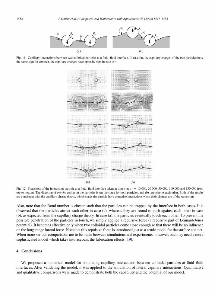
We consider two cases, (a) both particles are accelerated vertically in the same direction and (b) the particles areaccelerated vertically in the opposite direction to each other, the positive/positive and the positive/negative chargedpairs can thus be generated (see Fig. 11).

In Fig. 12, the snapshots taken from the simulation are shown for both cases. Note that the system had beenequilibrated for the first 10 000 time steps before applying the acceleration, in order to remove the density fluctuations.


Fig. 11. Capillary interactions between two colloidal particles at a fluid–fluid interface. In case (a), the capillary charges of the two particles havethe same sign. In contrast, the capillary charges have opposite sign in case (b).

Fig. 12. Snapshots of the interacting particle at a fluid–fluid interface taken at time steps t = 10 000, 20 000, 50 000, 100 000 and 150 000 fromtop to bottom. The direction of gravity acting on the particles is (a) the same for both particles, and (b) opposite to each other. Both of the resultsare consistent with the capillary charge theory, which states the particle have attractive interactions when their charges are of the same sign.

Also, note that the Bond number is chosen such that the particles can be trapped by the interface in both cases. It isobserved that the particles attract each other in case (a), whereas they are found to push against each other in case(b), as expected from the capillary charge theory. In case (a), the particles eventually touch each other. To prevent thepossible penetration of the particles in touch, we simply applied a repulsive force (a repulsive part of Lennard-Jonespotential). It becomes effective only when two colloidal particles come close enough so that there will be no influenceon the long-range lateral force. Note that this repulsive force is introduced just as a crude model for the surface contact.When more serious comparisons are to be made between simulations and experiments, however, one may need a moresophisticated model which takes into account the lubrication effects [19].

4. Conclusions

We proposed a numerical model for simulating capillary interactions between colloidal particles at fluid–fluidinterfaces. After validating the model, it was applied to the simulation of lateral capillary interactions. Quantitativeand qualitative comparisons were made to demonstrate both the capability and the potential of our model.


The advantage of our model will become much clearer, in particular, when motions of complex-shaped objectsare to be simulated, because the explicit tracking of the interfaces is unnecessary. Moreover, the effects of wettingproperties of the object surface can be incorporated in a physically appropriate manner. Thus, it can be expected asa promising model for a wide range of applications. For future work, we plan to extend the current model to threedimensions, and compare simulation results quantitatively with experimental or theoretical data.

References

[1] P.A. Kralchevsky, K. Nagayama, Capillary interactions between particles bound to interfaces, liquid films and biomembranes, Adv. ColloidInterface Sci. 85 (2000) 145–192.

[2] S. Chen, G.D. Doolen, Lattice Boltzmann method for fluid flows, Annu. Rev. Fluid Mech. 30 (1998) 329–364.[3] A.J.C. Ladd, Numerical simulations of particulate suspensions via a discretized Boltzmann equation. Part I. Theoretical foundation, J. Fluid

Mech. 271 (1994) 285–309.[4] A.J.C. Ladd, Numerical simulations of particulate suspensions via a discretized Boltzmann equation. Part II. Numerical results, J. Fluid Mech.

271 (1994) 311–339.[5] K. Stratford, R. Adhikari, I. Pagonabarraga, J.-C. Desplat, M.E. Cates, Colloidal jamming at interfaces: A route to fluid-bicontinuous gels,

Science 309 (2005) 2198–2201.[6] K. Stratford, R. Adhikari, I. Pagonabarraga, J.-C. Desplat, Lattice Boltzmann for binary fluids with suspended colloids, J. Stat. Phys. 121

(2005) 163–178.[7] X. Shan, H. Chen, Lattice Boltzmann model for simulating flows with multiple phases and components, Phys. Rev. E 47 (1993) 1815–1819.[8] L.-S. Luo, Theory of the lattice Boltzmann method: Lattice Boltzmann models for nonideal gases, Phys. Rev. E 62 (2000) 4982–4996.[9] N.S. Martys, H. Chen, Simulation of multicomponent fluids in complex three-dimensional geometries by the lattice Boltzmann method, Phys.

Rev. E 53 (1996) 743–750.[10] X. He, L. Luo, Theory of the lattice Boltzmann method: From the Boltzmann equation to the lattice Boltzmann equation, Phys. Rev. E 56

(1997) 6811–6817.[11] S. Chen, X. He, G.D. Doolen, A novel thermal model for the lattice Boltzmann method in incompressible limit, J. Comput. Phys. 146 (1998)

282–300.[12] Z. Guo, C. Zhen, B. Shi, Discrete lattice effects on the forcing term in the lattice Boltzmann method, Phys. Rev. E 65 (2002) 046308.[13] H. Tanaka, T. Araki, Simulation method of colloidal suspensions with hydrodynamic interactions: Fluid particle dynamics, Phys. Rev. Lett.

85 (2000) 1338–1341.[14] A.S. Sangani, A. Acrivos, Slow flow past periodic arrays of cylinders with application to heat transfer, Int. J. Multiphase Flow 8 (1982)

193–206.[15] M.W. Heemels, M.H.J. Hagen, C.P. Lowe, Simulating solid colloidal particles using the Lattice–Boltzmann method, J. Comput. Phys. 164

(2000) 48–61.[16] J.-P. Hansen, I.R. McDonald, Theory of Simple Liquids, 2nd ed., Academic Press, 1986.[17] W.A. Gifford, L.E. Scriven, On the attraction of floating particles, Chem. Eng. Sci. 26 (1971) 287–297.[18] V.N. Paunov, P.A. Kralchevsky, N.D. Denkov, K. Nagayama, Lateral capillary forces between floating submillimeter particles, J. Colloid

Interface Sci. 157 (1993) 100–112.[19] N.-Q. Nguyen, A.J.C. Ladd, Lubrication correction for lattice-Boltzmann simulations of particle suspensions, Phys. Rev. E 66 (2002) 046708.

Lattice Boltzmann simulation of capillary interactions among colloidal particles

Documents

Transcript of Lattice Boltzmann simulation of capillary interactions among colloidal particles