arX

iv:1

106.

2566

v1 [

cond

-mat

.sof

t] 1

3 Ju

n 20

11

On measuring colloidal volume fractions

Wilson C. K. PoonScottish Universities Physics Alliance (SUPA) and The School of Physics,

University of Edinburgh, Kings Buildings, Mayfield Road, Edinburgh EH9 3JZ, U. K.

Eric R. WeeksDepartment of Physics, Emory University, Atlanta, GA 30322 U.S.A.

C. Patrick RoyallSchool of Chemistry, University of Bristol, Bristol, BS8 1TS, U.K

Hard-sphere colloids are popular as models for testing fundamental theories in condensed matterand statistical physics, from crystal nucleation to the glass transition. A single parameter, thevolume fraction (φ), characterizes an ideal, monodisperse hard-sphere suspension. In comparingexperiments with theories and simulation, researchers to date have paid little attention to likelyuncertainties in experimentally-quoted φ values. We critically review the experimental measurementof φ in hard-sphere colloids, and show that while statistical uncertainties in comparing relative valuesof φ can be as low as 10−4, systematic errors of 3-6% are probably unavoidable. The consequencesof this are illustrated by way of a case study comparing literature data sets on hard-sphere viscosityand diffusion.

I. INTRODUCTION

Excluded volume effects dominate the behaviour ofliquids around the triple point [1] and play a key rolein structuring crystalline [2] and amorphous solids [3].Thus, hard spheres have long functioned as a referencesystem for theoretical and simulational studies of con-densed matter. In 1986, Pusey and van Megen demon-strated [4] that suspensions of sterically-stabilised poly-methylmethacrylate (PMMA) colloids showed nearly-perfect hard-sphere equilibrium phase behaviour, under-going a first-order phase transition from a fluid to a crys-talline state at concentrations around those predictedsome time ago by computer simulations for hard spher-ical particles [5, 6]. Soon afterward, the same authorsshowed [7] that PMMA colloids underwent a glass tran-sition at even higher concentrations. Subsequently, ina 1991 review, Pusey enunciated the ‘colloids as atoms’paradigm [8] — Brownian suspensions can be used as‘test tube simulations’ of many generic condensed mat-ter phenomena such as crystallization and vitrification.Since then, the use of colloids as models has become verypopular, especially since the addition of non-adsorbingpolymers can be used to induce an inter-particle attrac-tion ‘tuneable’ separately in its range and depth [9, 10].In such colloid-polymer mixtures, gas-liquid coexistencecan be studied [11, 12], including interfaces and critical-ity [13, 14], as well as novel modes of arrest [15]. Dueto their slow intrinsic time scales, colloids are also idealmodels for studying phase transition kinetics [16].

While a range of inter-particle interactions are nowavailable in model colloids, hard spheres remain an im-portant reference system for which very direct compari-son between experiments and theoretical calculations orcomputer simulations is in principle possible. The be-haviour of a single-sized, or monodisperse, system of hard

spheres is controlled by one parameter, the volume frac-tion φ, i.e. the fraction of the total volume V that isfilled by N spheres, each of radius a,

φ =4

3πa3

N

V. (1)

Since φ is precisely known in theory or simulations, acomparison with experiments is straightforward providedthat this quantity is also accurately measurable for realsuspensions. Much of the literature has indeed pro-ceeded on this basis, assuming that φ is unproblemati-cally known from experiments.However, as Pusey and van Megen pointed out in a

symposium article [17] following their Nature paper,[4]the experimental determination of φ is emphatically not

unproblematic, because: (1) no real colloid is truly‘hard’, since there is always some softness in the inter-particle potential; and (2) real colloids always have afinite size distribution, i.e. they are polydisperse. Thus,Pusey and van Megen calculated an experimental ‘ef-fective’ hard-sphere volume fraction φE, and found thatthe freezing and melting volume fractions of their systemwere 0.494 and 0.535 respectively, compared to 0.494 and0.545 in simulations.[5, 6] Their careful conclusion reads:‘Despite ambiguities . . . in the experimental determina-tion of the coexistence region this difference is probablysignificant.’The same degree of caution has not characterized the

literature since. Experimental reports typically do notdiscuss in any detail the method used for arriving at φ.On the other hand, theory or simulations almost alwaystake experimental reports of φ at face value and proceedto use the data on this basis. This is unsatisfactory, par-ticularly in situations where theory testing demands adegree of accuracy and certainty in the experimental φthat is probably unattainable. In this paper, we criticallyreview a plethora of methods for the experimental deter-

2

mination of φ in hard-sphere suspensions, evaluate thedegree of accuracy attainable in each case, comment onthe potential discrepancies between methods, and givea case study showing how different experiments shouldbe compared taking into account possible difference in φdetermination.With the increasing popularity of confocal microscopy,

direct counting of particles is becoming a standardmethod for determining φ (see Sec. VD). This methoddepends on knowing the particle size. Thus, after in-troducing model colloids (Section II), we review particlesizing (Section III). The ‘classic’ method for determin-ing φ is via the crystallization phase behaviour, whichchanges with polydispersity[18, 19]. So we review poly-dispersity measurements (Section IV) before turning toconsider the determination of φ in detail (Section V). Wefinish with a case study (Section VI) and a Conclusion.

II. THE PARTICLES

We focus on suspensions of nearly-perfect hard spheres.A system that potentially behaves most like perfecthard spheres is charge-stabilised colloidal silica in wa-ter. When the charges are sufficiently screened out bythe addition of salt [20–22], the resulting suspension isvery close to being hard-sphere-like. However, a signifi-cant drawback of silica as a model system is that theseparticles have a density ρ ≈ 2.2 g/cm3, and it has provedimpossible to find solvents that match this density. Thesedimentation problem can be alleviated by using smallerparticles, but at the expense of increasing polydisper-sity. Charged-stabilised polystyrene spheres are also po-tentially very hard-sphere-like, and are easier to densitymatch, though (unlike silica) almost impossible to refrac-tive index match.A more popular model hard sphere system is PMMA,

sterically stabilized by a δ . 10 nm layer of PHSA (poly-12-hydroxystearic acid) [23]. This layer confers a degreeof softness to the interparticle potential on the scale ofδ. PMMA particles can be dispersed in solvent mixturesthat match both the particles’ density and index of re-fraction [24, 25]. Unfortunately, particle swelling by sol-vents is endemic [26, 27]. Furthermore, the swelling pro-cess can take several weeks, so the particle size changesover time, though heat shock may speed up the processto taking only a few hours [28]. As swelling is poorlycharacterized, in situ measurement is the only reliablemeans of ensuring that it is complete before the parti-cles are used in experiments. This is particularly impor-tant at high φ, where many properties are steep func-tions of the concentration: an x% increase in the particleradius translates into & 3x% in φ. Thus, e.g., an index-matching mixture of cis-decalin and tetrachloroethylenecauses 20% swelling, which has a drastic effect upon thecolloid volume fraction [27]. Finally, batch-to-batch vari-ations generate further uncertainties.Below, we focus on PMMA particles, although much

δ=

(a) (b)

acs acacacs

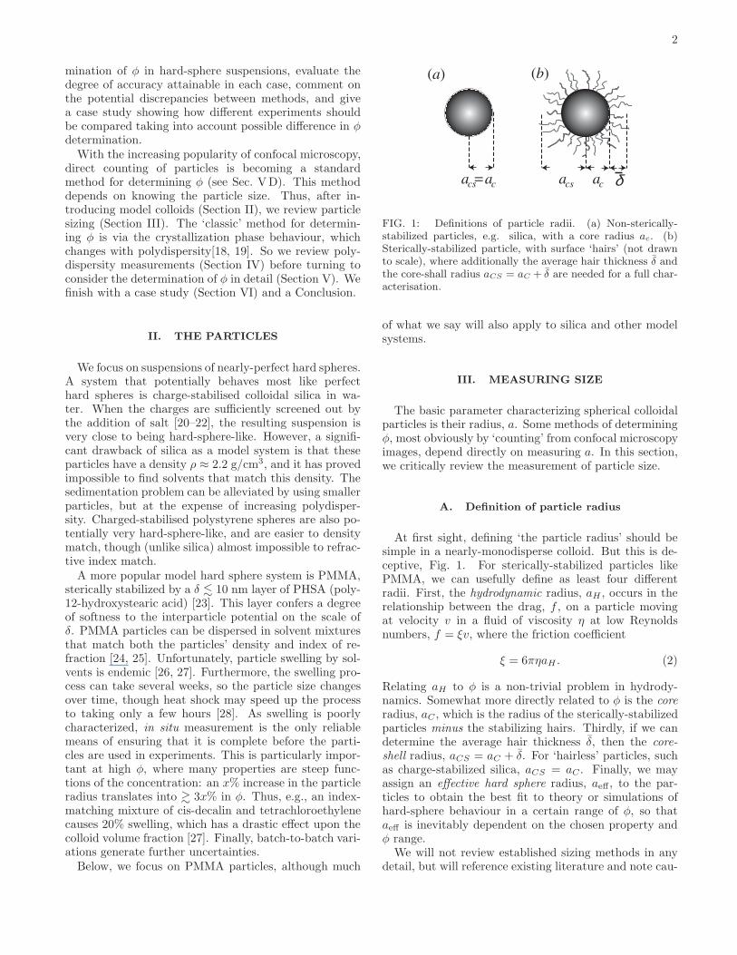
FIG. 1: Definitions of particle radii. (a) Non-sterically-stabilized particles, e.g. silica, with a core radius ac. (b)Sterically-stabilized particle, with surface ‘hairs’ (not drawnto scale), where additionally the average hair thickness δ andthe core-shall radius aCS = aC + δ are needed for a full char-acterisation.

of what we say will also apply to silica and other modelsystems.

III. MEASURING SIZE

The basic parameter characterizing spherical colloidalparticles is their radius, a. Some methods of determiningφ, most obviously by ‘counting’ from confocal microscopyimages, depend directly on measuring a. In this section,we critically review the measurement of particle size.

A. Definition of particle radius

At first sight, defining ‘the particle radius’ should besimple in a nearly-monodisperse colloid. But this is de-ceptive, Fig. 1. For sterically-stabilized particles likePMMA, we can usefully define as least four differentradii. First, the hydrodynamic radius, aH , occurs in therelationship between the drag, f , on a particle movingat velocity v in a fluid of viscosity η at low Reynoldsnumbers, f = ξv, where the friction coefficient

ξ = 6πηaH . (2)

Relating aH to φ is a non-trivial problem in hydrody-namics. Somewhat more directly related to φ is the core

radius, aC , which is the radius of the sterically-stabilizedparticles minus the stabilizing hairs. Thirdly, if we candetermine the average hair thickness δ, then the core-

shell radius, aCS = aC + δ. For ‘hairless’ particles, suchas charge-stabilized silica, aCS = aC . Finally, we mayassign an effective hard sphere radius, aeff , to the par-ticles to obtain the best fit to theory or simulations ofhard-sphere behaviour in a certain range of φ, so thataeff is inevitably dependent on the chosen property andφ range.We will not review established sizing methods in any

detail, but will reference existing literature and note cau-

3

tionary points. Then we will introduce a number of newermethods.

B. Measuring radius: established methods

Scattering methods have a long history in sizing spheri-cal particles[29–31]. Static and dynamic scattering deter-mine the size of particles by measuring the time-averagedor fluctuating intensity of the scattered light respectively.Dynamic light scattering (DLS) and its X ray equiv-

alent, X ray photon correlation spectroscopy (XPCS),measure the diffusion coefficient of particles, which is re-lated to the friction coefficient via the Stokes-Einstein-Sutherland relation[32–34]: D = kBT/ξ. DLS and XPCStherefore determine aH (cf. Eqn. 2), and are most usefulin the case of particles consisting of core only, such as sil-ica, since it is less clear how to relate aH to aCS for core-shell particles such as PMMA. Note that the accuracyof this method depends on having an accurate value forη, the solvent viscosity, which is temperature dependent.For example, we have found that for the common sol-vent mixture cyclohexylbromide and decalin (85%/15%by weight) 24◦C, η = 2.120 mPa·s and dη/dT = −0.029mPa·s/K. Thus, a 1◦C uncertainly in T is a 0.3% uncer-tainty of T but a 1.7% uncertainty in T/η and thereforein aH .Static light scattering (SLS), small-angle X ray scat-

tering (SAXS) or small-angle neutron scattering (SANS)can potentially determine aC and aCS. Since the coreand shell of (say) a PMMA particle in general has differ-ent contrasts to light, X rays (refractive index, n, in bothcases) and neutrons (scattering length, b), the diffractionpattern of a single particle is determined by the interfer-ence of radiation scattered from these two parts. Fittingthis diffraction pattern (the form factor) therefore canin principle yield aC and aCS = aC + δ. In a solventwith n or b quite different from both the core and theshell, the whole entity scatters more or less as a homoge-neous sphere and a radius close to aCS is returned fromform-factor fitting. When solvent mixtures are used to‘tune’ the relative contrasts of core and shell, even a smallamount of a minority component in the solvent mixturecan swell the particles by up to 10% or more[26, 27], andthe fractional swelling of core and shell is not necessarilyidentical. In XPCS, where the shell has little contrast,δ cannot be accurately determined; however, the bright-ness of the beam gives many orders of oscillations in theform factor, allowing very accurate data fitting.For both static and dynamic scattering, samples must

be dilute enough so that the properties of non-interactingparticles are measured in the single-scattering limit. Theonly sure way to know that this has been achieved is tocollect data at different φ and look for the convergencein the φ → 0 limit. Static scattering at finite φ gives thestatic structure factor as a function of scattering vector,S(q). Fitting this to, e.g., the Percus-Yevick form [35]or simulations yields simultaneously aeff and φ, although

polydispersity is a significant complication[36]. Alterna-tively, the Bragg peaks in S(q) from colloidal crystals atfluid-crystal coexistence can be used to deduce aeff if themelting point is known (but see Section IV for caveats).Electron microscopy (EM) measures aC of dried parti-

cles, because drying collapses the steric-stabilizing ‘hairs’in core-shell particles such as PMMA, and deswells par-ticles swollen by solvent when dispersed. Various opticalmicroscopies can, in principle, be used in the same wayas EM for sizing particles; caveats are pointed out inSection III D.

C. Measuring radius: newer methods

1. Differential dynamic microscopy

DLS measures diffusion via determining the intermedi-ate scattering function (ISF), which is the spatial Fouriertransform of a time-dependent density-density correla-tion function[29–31]; it requires a laser and bespoke elec-tronics (a correlator). Recently, a method for measuringthe ISF has been demonstrated[37] that requires only theuse of everyday laboratory equipment, viz., a white-lightoptical microscope and a CCD camera. This method, dif-ferential dynamic microscopy (DDM), exploits the factthat the intensity of a low-resolution microscope imag-ing is linearly related to the density of particles in thesample being imaged[38]. Thus, correlating the Fouriertransform of the images gives directly the ISF.

2. Particle tracking

Being a scattering method, DLS works in reciprocalspace. DDM uses microscope images, but also yields theISF in reciprocal space. In both cases, the measuredquantity is the diffusion coefficient, which controls themean-squared displacement (MSD) of Brownian parti-cles: 〈∆r2(τ)〉 = nDτ , with n = 2, 4 or 6 in 1, 2 or 3dimensions respectively. Direct real-space methods formeasuring the MSD are increasingly popular. The mo-tion of particles in a dilute sample (φ ≪ 0.01) can be cap-tured by video microscopy[39], and the particle motiontracked[40] using publicly available software[41]. Pro-vided the microscope has been properly calibrated, suchtracks yield the MSD.Problems can occur at short and long times. The issue

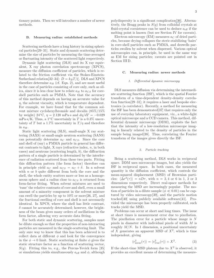
at short times is measurement error due to pixellation.The pixellation error for a particle whose image is Npixels in diameter with individual pixels of width M isroughly M/N . In 1 dimension, a positional uncertaintyof X generates an apparent MSD of X2, which is timeindependent, giving

〈r2meas(τ)〉 = 〈r2true(τ)〉 +X2. (3)

If the short-time MSD plateau due to X2 is observed, itprovides an excellent means of determining the measure-

4

FIG. 2: Mean square displacement of aC = 1.5 µmpolystyrene spheres in a water-glycerol mixture. (◦): rawdata; (+): 〈∆x2〉−X2 where the estimated noise level (dashedline) is X = 0.08 µm. Solid line: a linear fit to the raw datain the range 100 < τ < 101 s, giving D = 0.0254 µm2/s.With the noise subtracted off, a linear fit to all of the dataat τ < 101 s gives D = 0.0248 µm2/s. In this experiment,N = 9 and M = 0.64 µm/pixel, so the estimated noise levelM/N = 0.07 µm is comparable to the observed X = 0.08 µm.

ment uncertainty X . Figure 2 shows that it is importantto take this term into account for accurate determinationof D by tracking. Note that changing the parametersused to identify particle positions can often influence X ,for better or worse [40].At long times, the measured MSD can become non-

linear due to particles disappearing from the field of view,either because they leave laterally or because they be-come defocussed. Since the MSD at any τ is computedbased only on particles which have been observed for atleast as long as τ , too few particles may contribute atlarge τ for proper averaging.

3. Confocal microscopy

By using a pinhole to reject out-of-focus light, laserconfocal microscopy is capable of generating images deepinside (∼ 100µm) a concentrated suspension of fluores-cent colloids. Thus, by processing images taken scan-ning through a sample, a 3 dimensional image of manythousands of particles can be reconstructed and their co-ordinates obtained[41, 42]. In a sample where particlesare touching, the peak of the calculated radial distribu-tion function, g(r), gives aCS . Touching particles canbe generated in a spun-down sediment[43], or by induc-ing a very short range attraction (e.g. by adding smallnon-adsorbing polymers). While the first peak of g(r)is typically averaged over & 108 correlations, and so isin principle highly accurate, the particle size in a typi-cal confocal image is . 10 pixels, which limits the bestaccuracy to ∼ 0.1 pixel. Furthermore, microscopy is sub-ject to certain systematic errors [44, 45] that affect the

determination of g(r). Finally, note that the scanningmechanism drifts, so that calibration on the day of mea-surement is important.

4. Holographic microscopy

A collimated laser beam directed through a microscopeobjective scatters off a particle. The scattered and un-scattered beams interfere in the focal plane to form ahologram. At low enough φ, the holographic image of asingle, optically homogeneous particle can be fitted usingLorenz-Mie theory to determine its position, size, and re-fractive index[46–48]. This has been demonstrated with∼ 100 nm to 10 µm particles. The radius aC of an indi-

vidual particle can be measured to ±10− 30 nm from asingle snapshot [49]. Multiple measurements further im-prove on this [48]. The sizing of core-shell particles hasnot yet been attempted. Note that while this methodfails for exactly index-matched particles, a mismatch ofas little as 1% is sufficient to render it usable (D. Grier,personal communication).

D. Measuring radius: case study

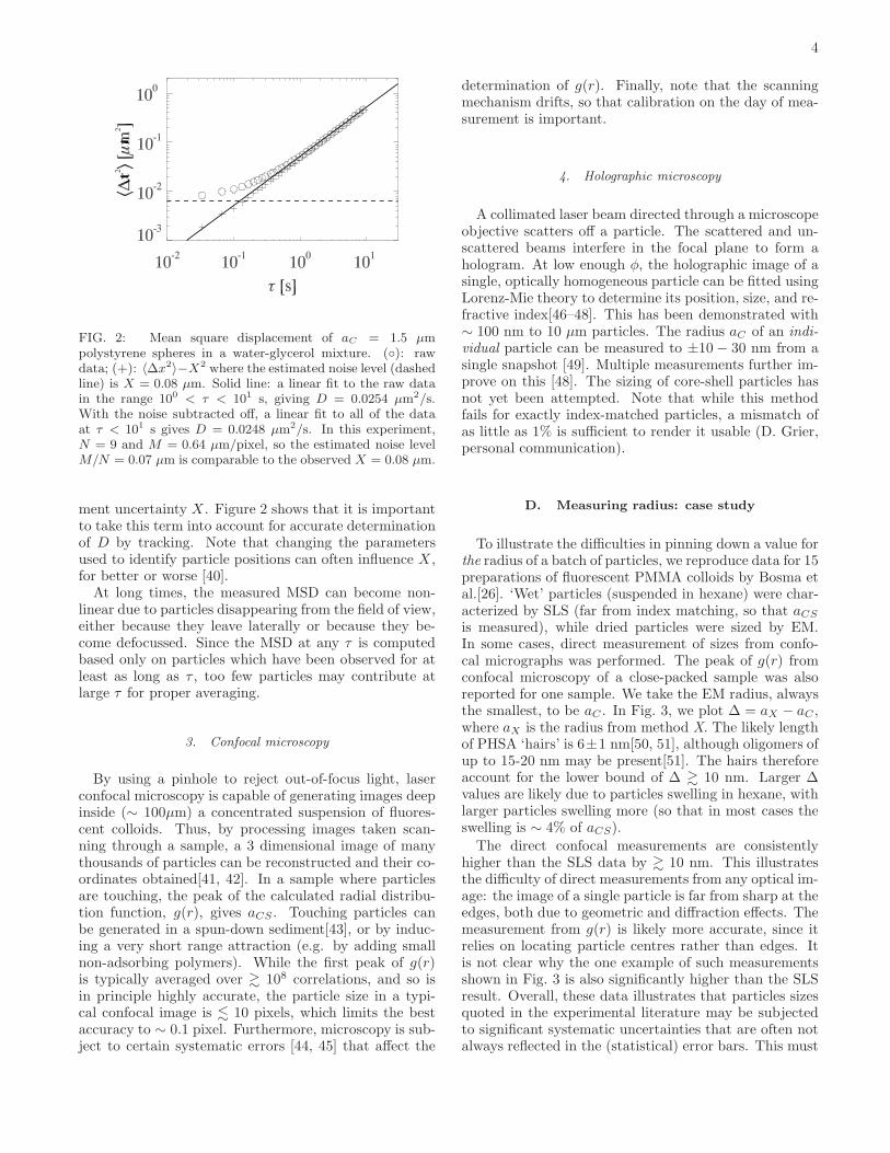
To illustrate the difficulties in pinning down a value forthe radius of a batch of particles, we reproduce data for 15preparations of fluorescent PMMA colloids by Bosma etal.[26]. ‘Wet’ particles (suspended in hexane) were char-acterized by SLS (far from index matching, so that aCS

is measured), while dried particles were sized by EM.In some cases, direct measurement of sizes from confo-cal micrographs was performed. The peak of g(r) fromconfocal microscopy of a close-packed sample was alsoreported for one sample. We take the EM radius, alwaysthe smallest, to be aC . In Fig. 3, we plot ∆ = aX − aC ,where aX is the radius from method X. The likely lengthof PHSA ‘hairs’ is 6±1 nm[50, 51], although oligomers ofup to 15-20 nm may be present[51]. The hairs thereforeaccount for the lower bound of ∆ & 10 nm. Larger ∆values are likely due to particles swelling in hexane, withlarger particles swelling more (so that in most cases theswelling is ∼ 4% of aCS).

The direct confocal measurements are consistentlyhigher than the SLS data by & 10 nm. This illustratesthe difficulty of direct measurements from any optical im-age: the image of a single particle is far from sharp at theedges, both due to geometric and diffraction effects. Themeasurement from g(r) is likely more accurate, since itrelies on locating particle centres rather than edges. Itis not clear why the one example of such measurementsshown in Fig. 3 is also significantly higher than the SLSresult. Overall, these data illustrates that particles sizesquoted in the experimental literature may be subjectedto significant systematic uncertainties that are often notalways reflected in the (statistical) error bars. This must

5

FIG. 3: Radii of different batches of fluorescent PMMA par-ticles determined by various methods[26]: • static light scat-tering, N confocal microscopy, � g(r) peak.

be taken into account if the particle size is then used incalculating φ.

IV. MEASURING POLYDISPERSITY

Polydispersity in general refers to the existence of adistribution of particle properties, such as size, shape,charge, magnetic moment, etc. Hard sphere colloids havea distribution of radii, P (a), for which we define the poly-dispersity, σ, as the standard deviation of this distribu-tion divided by the mean:

σ =(

〈a2〉 − 〈a〉2)1/2

/〈a〉. (4)

Very monodisperse PMMA has polydispersities ap-proaching 3%, however 5-6% is typical [26] for ‘monodis-perse’ PMMA. Note that some particles, includingPMMA, frequently display a bimodal distribution due tosecondary nucleation, so that a full distribution is neededto characterize them.Polydispersity is relevant here because it affects the

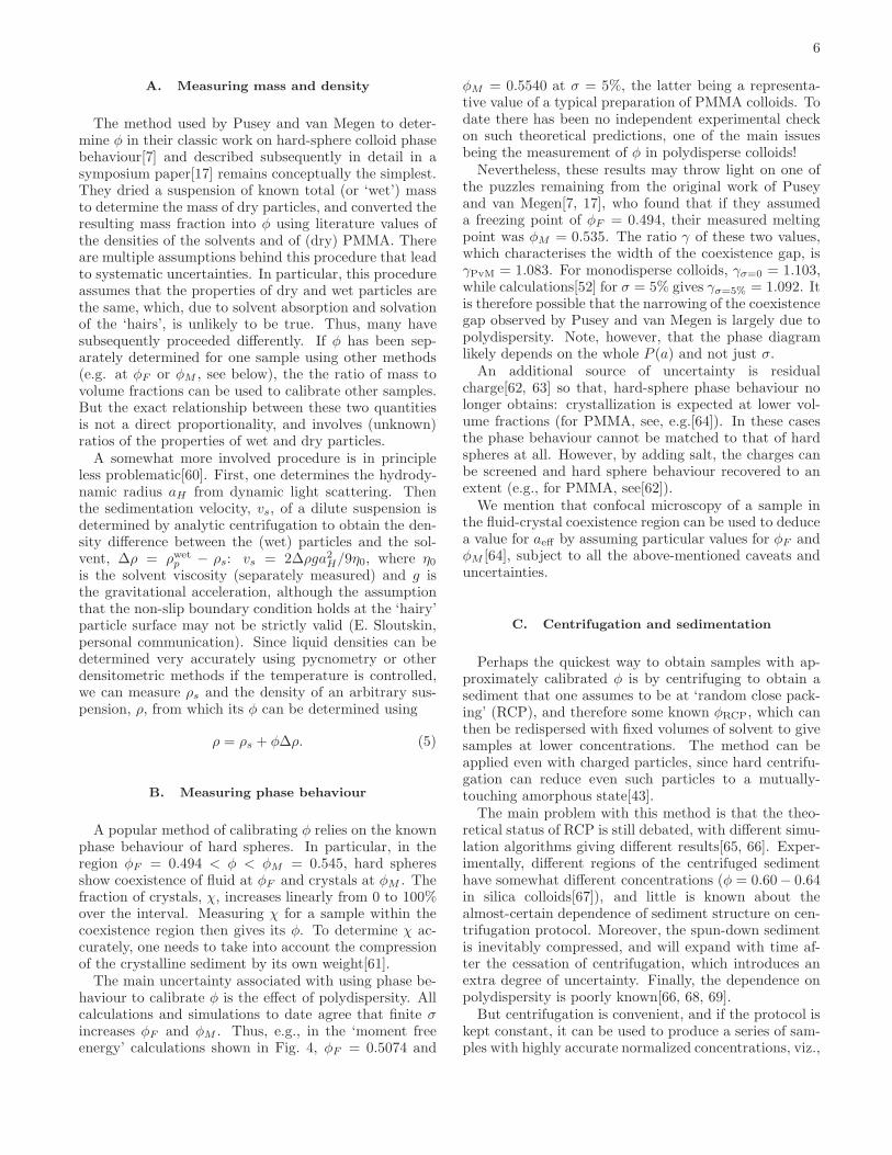
equilibrium phase diagram. Monodisperse hard spheresfreeze at φF = 0.494 to form crystals at the melt-ing point φM = 0.545. These two values are oftenused as fixed points for determining φ in experiments(see Section VB). Theory [18, 19, 52] and simula-tions [19, 52, 53] show that even small σ may shift φM

and/or φF significantly, Fig. 4. Indeed, particles withσ higher than some terminal value σ∗ will fail to crys-tallize at all experimentally or in simulations, althoughtheory[18] predicts phase separation into coexisting solidphases. Simulations[54] predict that σ∗ ≈ 7%, consistentwith early experiments[55]. Determining polydispersityis therefore important for measuring φ. Note that thewhole distribution and not just its variance may matter,e.g. in determination nucleation rates[56].All the methods reviewed in the last section can po-

tentially yield information on the size distribution. Di-rect imaging, EM or optical microscopy, can estimate the

FIG. 4: The theoretical phase diagram of hard spheres atdifferent polydispersities, σ. F = fluid, S = (crystalline)solid; thus FSS denotes fluid-solid-solid coexistence. Replot-ted from[52].

full P (a), subject to the same caveats already discussed.Moreover, larger particles may swell more (Fig. 3; seealso [48]), giving a correlation between size and shrinkageupon drying, so that wet and dry P (a) may be different.

In DLS or XPCS, the ISF from a hypotheticalmonodisperse suspension decays exponentially with time.Polydispersity turns the ISF into a sum of exponentials.In static scattering, monodisperse particles give sharpminima in the form factor, which are smeared out bypolydispersity. (Note that multiple scattering has thesame effect, and so can masquerade as polydispersity.) Inprinciple, these features can be fitted to yield P (a)[29],subject to all the usual problems and uncertainties as-sociated with solving an inverse problem. For DLS (orXPCS), there are well known algorithms such as CON-TIN [57] for backing out P (a) via the distribution ofdecay times in the ISF. Or, less ambitiously, cumulantanalysis[58] can be used to extract σ. Form factors fromstatic scattering are seldom inverted directly to yieldP (a). Instead, one assumes, say, a Gaussian form, andthe scattering profile from Mie theory is fitted to obtain〈a〉 and σ. The effect of small polydispersities (a few %)on the ISF and form factor can be treated analytically[59], and becomes independent of the form of P (a) asσ → 0. The resulting expressions can be used to fit dy-namic or static scattering data to yield rather accuratevalues of σ.

V. MEASURING VOLUME FRACTION

We now turn to describe and evaluate a number ofmethods for determining the volume fraction of modelcolloids.

6

A. Measuring mass and density

The method used by Pusey and van Megen to deter-mine φ in their classic work on hard-sphere colloid phasebehaviour[7] and described subsequently in detail in asymposium paper[17] remains conceptually the simplest.They dried a suspension of known total (or ‘wet’) massto determine the mass of dry particles, and converted theresulting mass fraction into φ using literature values ofthe densities of the solvents and of (dry) PMMA. Thereare multiple assumptions behind this procedure that leadto systematic uncertainties. In particular, this procedureassumes that the properties of dry and wet particles arethe same, which, due to solvent absorption and solvationof the ‘hairs’, is unlikely to be true. Thus, many havesubsequently proceeded differently. If φ has been sep-arately determined for one sample using other methods(e.g. at φF or φM , see below), the the ratio of mass tovolume fractions can be used to calibrate other samples.But the exact relationship between these two quantitiesis not a direct proportionality, and involves (unknown)ratios of the properties of wet and dry particles.A somewhat more involved procedure is in principle

less problematic[60]. First, one determines the hydrody-namic radius aH from dynamic light scattering. Thenthe sedimentation velocity, vs, of a dilute suspension isdetermined by analytic centrifugation to obtain the den-sity difference between the (wet) particles and the sol-vent, ∆ρ = ρwet

p − ρs: vs = 2∆ρga2H/9η0, where η0is the solvent viscosity (separately measured) and g isthe gravitational acceleration, although the assumptionthat the non-slip boundary condition holds at the ‘hairy’particle surface may not be strictly valid (E. Sloutskin,personal communication). Since liquid densities can bedetermined very accurately using pycnometry or otherdensitometric methods if the temperature is controlled,we can measure ρs and the density of an arbitrary sus-pension, ρ, from which its φ can be determined using

ρ = ρs + φ∆ρ. (5)

B. Measuring phase behaviour

A popular method of calibrating φ relies on the knownphase behaviour of hard spheres. In particular, in theregion φF = 0.494 < φ < φM = 0.545, hard spheresshow coexistence of fluid at φF and crystals at φM . Thefraction of crystals, χ, increases linearly from 0 to 100%over the interval. Measuring χ for a sample within thecoexistence region then gives its φ. To determine χ ac-curately, one needs to take into account the compressionof the crystalline sediment by its own weight[61].The main uncertainty associated with using phase be-

haviour to calibrate φ is the effect of polydispersity. Allcalculations and simulations to date agree that finite σincreases φF and φM . Thus, e.g., in the ‘moment freeenergy’ calculations shown in Fig. 4, φF = 0.5074 and

φM = 0.5540 at σ = 5%, the latter being a representa-tive value of a typical preparation of PMMA colloids. Todate there has been no independent experimental checkon such theoretical predictions, one of the main issuesbeing the measurement of φ in polydisperse colloids!Nevertheless, these results may throw light on one of

the puzzles remaining from the original work of Puseyand van Megen[7, 17], who found that if they assumeda freezing point of φF = 0.494, their measured meltingpoint was φM = 0.535. The ratio γ of these two values,which characterises the width of the coexistence gap, isγPvM = 1.083. For monodisperse colloids, γσ=0 = 1.103,while calculations[52] for σ = 5% gives γσ=5% = 1.092. Itis therefore possible that the narrowing of the coexistencegap observed by Pusey and van Megen is largely due topolydispersity. Note, however, that the phase diagramlikely depends on the whole P (a) and not just σ.An additional source of uncertainty is residual

charge[62, 63] so that, hard-sphere phase behaviour nolonger obtains: crystallization is expected at lower vol-ume fractions (for PMMA, see, e.g.[64]). In these casesthe phase behaviour cannot be matched to that of hardspheres at all. However, by adding salt, the charges canbe screened and hard sphere behaviour recovered to anextent (e.g., for PMMA, see[62]).We mention that confocal microscopy of a sample in

the fluid-crystal coexistence region can be used to deducea value for aeff by assuming particular values for φF andφM [64], subject to all the above-mentioned caveats anduncertainties.

C. Centrifugation and sedimentation

Perhaps the quickest way to obtain samples with ap-proximately calibrated φ is by centrifuging to obtain asediment that one assumes to be at ‘random close pack-ing’ (RCP), and therefore some known φRCP, which canthen be redispersed with fixed volumes of solvent to givesamples at lower concentrations. The method can beapplied even with charged particles, since hard centrifu-gation can reduce even such particles to a mutually-touching amorphous state[43].The main problem with this method is that the theo-

retical status of RCP is still debated, with different simu-lation algorithms giving different results[65, 66]. Exper-imentally, different regions of the centrifuged sedimenthave somewhat different concentrations (φ = 0.60− 0.64in silica colloids[67]), and little is known about thealmost-certain dependence of sediment structure on cen-trifugation protocol. Moreover, the spun-down sedimentis inevitably compressed, and will expand with time af-ter the cessation of centrifugation, which introduces anextra degree of uncertainty. Finally, the dependence onpolydispersity is poorly known[66, 68, 69].But centrifugation is convenient, and if the protocol is

kept constant, it can be used to produce a series of sam-ples with highly accurate normalized concentrations, viz.,

7

φ/φsed, where φsed is the volume fraction of the sediment.Under this heading, we may mention that particles

with small enough gravitational Peclet number[43, 70](either by virtue of near density matching or by virtueof being small) and low enough polydispersity will sedi-ment slowly under gravity to form sedimentary crystalsconsisting of more or less randomly-stacked hexagonalclose packed (rhcp) layers of particles. If the particles are

monodisperse hard spheres, then φrhcp = π/√18 ≈ 0.74

in this sediment. Again, however, the (largely unknown)effect of polydispersity as well as any changes due tocharges need to be taken into account.

D. Confocal microscopy and particle counting

Confocal microscopy can be used to locate the posi-tion of thousands of particles in a suspension. Thus, ifthe particle radius, a, is known, then counting N par-ticle in an imaging volume V will yield φ directly usingEqn. 1. Occasional particle mis-identification or missinga particle all together by the software give rise to erro-neous φ, so that it is important to cross-check particlepositions identified against raw images. In particular,particles near the edge of images are often mis-identified,so that in practice a sub-volume only is considered. Fi-nally, uncertainties in a are magnified 3-fold or more incalculating φ. This latter uncertainty is compounded bythe issue of which of the possible radii (Section IIIA) oneshould use.

E. X-ray transmission

The intensity of X rays transmitted by a sample isgiven by IT = I0e

−µx, where I0 is the incident inten-sity, µ and x are the attenuation coefficient and thick-ness of the sample. In the case of a colloidal suspension,µ = (1−φ)µs+φCµp, where φC is the volume fraction ofparticle cores, and µs and µp are the attenuation coeffi-cients of the solvent and particles. The negligible amountof electron density represented by sterically-stabilizing‘hairs’ means that they hardly contribute to the beamattenuation. X ray transmission can therefore be used todetermine φ directly for model colloids such as charge-stabilised polystyrene [71] or silica[72], but only the corevolume fraction for sterically-stabilised particles.

F. Measuring φ-dependent properties

The φ-dependence of a number of material propertiesof hard-sphere suspensions are known either from ana-lytic theory or highly-accurate simulations. In principle,therefore, measuring these properties can be used to de-termine φ. Here we review three: viscosity, diffusivityand structure factor.

Einstein predicted that in the limit φ → 0, the vis-cosity of a hard-sphere suspension is given by η(φ)/η0 =1+(5/2)φ, with η0 being the viscosity of the solvent [34].Thus, in principle, measuring η(φ) is a method for deter-mining φ (e.g.[73]). While suspensions in general shearthin, this should not be a problem in the very dilutelimit. But temperature control is important, since η0 istemperature sensitive (cf. Section III B).The problems associated with this method have been

detailed before[74]. In essence, very low φ, certainly. 0.02, must be reached for the Einstein result to bevalid; otherwise, second[75, 76] and higher order term inthis ‘virial’ expansion needs to be taken into account. Inthe case cited[73], using the Einstein relation at φ ≈ 3%leads to an error in φ of ≈ 7%[74]. The difficulty, ofcourse, is that in the limit φ → 0, very accurate viscom-etry is needed to distinguish the dilute suspension frompure solvent. Using the Einstein relation to calibrate φin suspensions that are too concentrated for the relationto be valid accounts for some of the spread in literaturevalues of η(φF ), the viscosity of the most concentratedstable fluid state of hard spheres. Interestingly, determin-ing φ using the Einstein relation is strictly independentof polydispersity: in the dilute limit, each particle con-tributes by an additive amount that is proportional to itsvolume.Instead of measuring η(φ), one could determine the

single-particle diffusion coefficient as a function of φ.Thus, El Masri et al.[77] measured the short-time self dif-fusion coefficient as a function of volume fraction, Ds

s(φ).The difficulty is that there are at least two different pre-dictions for this behaviour [78, 79] which leads to a 7%absolute uncertainty in φ.Lastly, we have already mentioned (Section III B) that

analytical expressions for the static structure factor,S(q), of hard spheres are available. In particular, theclosed-form expression from the Percus-Yevick (PY) ap-proximation [35] fits simulation data closely, providedthat the empirical Verlet-Weis correction to the volumefraction[80] is applied, i.e. the PY structure factor forvolume fraction φ′ is used for an experimental sample atφ: φ′ = φ−φ2/16. Thus, fitting measured S(q) can yielda measure of φ, provided that the particles can be treatedas hard spheres. Again, caution about residual chargesapplies. Alternatively, g(r) determined from confocal mi-croscopy can be fitted to the PY form or to simulationdata[81] to give φ.

G. Deceptive samples

Finally, we explain how using an accurately calibrated‘stock colloid’ may still lead to errors in the φ of samples.First, we have already mentioned a number of times the

issue of swelling. If particles used for calibrating volumefraction are still in the process of swelling due to solventabsorption, then samples prepared subsequently will havea higher φ than the earlier calibration would suggest.

8

Secondly, preparing samples almost invariably involvestransferring suspension from one container (e.g. a bot-tle of stock) to another (e.g. a capillary for microscopy)using (typically) a pipette or a syringe. Apart from dif-ficulties caused by very high viscosities[22] and shearthickening[82, 83], there is the problem of jamming ofthe particles as the suspension enters a constriction[84],which leads to a ‘self filtration’ effect. Particles jammedat (say) the entrance to a pipette prevents other particlesfrom entering, but solvent continues to flow, so that thesample inside the pipette has a lower φ than the bulksuspension that we hope to transfer. Thus, a sampleloaded for confocal microscopy may be more dilute thanone expects.

Thirdly, except for very well density-matched sam-ples at a temperature accurately remaining at the tem-perature at which the density matching was originallyachieved, suspension inevitably sediment (or cream) withtime at all except φRCP or φrhcp. This will lead to con-centration gradients. Indeed, such gradients can be de-liberated exploited[43, 64, 72, 85–87], e.g. to determineequations of state. But in other cases, concentration gra-dients lead to unintended local deviations from the av-erage φ at which the sample as a whole was originallyprepared.

Since one of the most important uses of hard-spherecolloids is as a model to study dynamical arrest[15, 88, 89]and associated properties such as aging[90, 91], any of theabove three sources of unintended changes in φ will havesevere consequences: all suspension properties changevery rapidly with φ at and above the glass transition(φ & 0.58).

H. Summary: relative vs. absolute φ

The most important message from the preceding crit-ical review is that the statistical errors involved in de-termining φ in the competent use of any of the abovemethods can almost certainly be brought below the sys-

tematic errors involved. Thus, for example, if one usesconfocal microscopy to count particles and thus deter-mine φ, the major source of uncertainty is likely to be theinput radius. Thus, it is perfectly possible to produce aseries of samples with relative uncertainty in φ of 1 partin 104. However, our collective experience in using manyof these methods suggests that the systematic uncertain-ties are unlikely to be below 3-6%. Far from being asmall error, such uncertainties can have dramatic effects.Thus, e.g., the viscosity of a hard-sphere suspension[74]grows by a factor of 2 when φ increases from 0.47 to 0.49;and the simulated crystal nucleation rate[94] near φF canchange by 10 orders of magnitude for a 1% change in theabsolute value of φ.

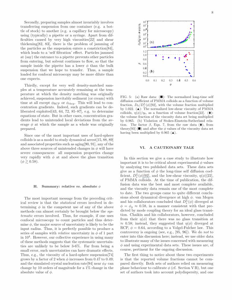
FIG. 5: (a) Raw data: (�): The normalized long-time selfdiffusion coefficient of PMMA colloids as a function of volumefraction, D0/D

Ls (φ)[92], with the volume fraction multiplied

by 1.022. (N): The normalized low-shear viscosity of PMMAcolloids, η(φ)/η0, as a function of volume fraction[22]. (�):the volume fraction of the viscosity data set being multipliedby 0.965. (b) Violation of Stokes-Einstein-Sutherland rela-tion. The factor β, Eqn. 7, from the raw data (�), fromtheory[93] (�) and after the φ values of the viscosity data sethaving been multiplied by 0.965 (N).

VI. A CAUTIONARY TALE

In this section we give a case study to illustrate howimportant it is to be critical about experimental φ valuesby analyzing two published data sets. These data setsgive as a function of φ the long-time self diffusion coef-ficient, DL

s (φ)[92], and the low-shear viscosity, η(φ)[22],of PMMA colloids. At the time of publication, the dif-fusion data was the best and most complete available,and the viscosity data remain one of the most completeto date. The two groups came to quite different conclu-sions about dynamical divergence at high φ. van Megenand his collaborators concluded that DL

s (φ) diverged atφ = φg ≈ 0.58, in a manner consistent with that pre-dicted by mode coupling theory for an ideal glass transi-tion. Chaikin and his collaborators, however, concludedfrom their η(φ) that there was no glass transition at≈ 0.58; instead, they suggested that η(φ) diverged atRCP, φ = 0.64, according to a Volgel-Fulcher law. Thiscontroversy is ongoing (see, e.g., [95, 96]). We do not toenter into this discussion here; instead, we use older datato illustrate many of the issues concerned with measuringφ and using experimental data sets. These issues are, ofcourse, pertinent for the ongoing discussion.

The first thing to notice about these two experimentsis that the reported volume fractions cannot be com-pared directly. Both sets of authors relied on measuringphase behaviour to calibrate φ (cf. Section VB), but oneset of authors took into account polydispersity, and one

9

did not. van Megen and co-workers used φF = 0.494,the value for monodisperse hard spheres, to determineφ, but cautioned that their particles had a polydisper-sity of σ = 5%. The colloids used by Chaikin and hisco-workers also had the same σ, and they used the sim-ulation data of Bolhuis and Kofke [53] to move freezingto φF = 0.505 for this polydispersity. Interestingly, thelatest analytic calculations agree closely: Wilding andSollich[52] give φF = 0.5074 at σ = 5%, Fig. 4. Thus,we multiply the φ value of the van Megen data set by afactor of 0.505/0.494 = 1.022 to make it consistent withthe Chaikin φ values. The resulting data are shown inFig. 5. The measurements have been normalised, DL

s (φ)by the single-particle diffusivity, D0, and η(φ) by the sol-vent viscosity, η0. The normalized viscosity diverges athigher φ than the normalized (inverse) diffusivity.At φ → 0, the solvent viscosity and the single-particle

diffusivity are related by the Stokes-Einstein-Sutherlandrelation (SESR): D0 = kBT/6πη0a. At finite φ, there isno a priori reason that a generalized SESR should holdfor any of the many diffusion coefficients that can bedefined. So we write

DLs (φ) =

kBT

6πη(φ)a× β (6)

where β is a numerical factor that can be restated as

β =DL

s (φ)

D0

× η(φ)

η0(7)

We plot in Fig. 5(b) (diamonds) the β(φ) implied by thedata sets in Fig. 5(a). In so far as β 6= 1, the SESR isviolated.Violation of the SESR is widely known for glass-

forming systems near the glass transition. In all experi-mental cases known (see e.g.[97]), β > 1, i.e. the particlesdiffuse somewhat faster than the viscosity allows accord-ing to the SESR. The fact that β drops very substantiallybelow unity at φ & 0.4 in Fig. 5(b) is therefore surprising,and merits further analysis.To proceed, we turn to the work of Banchio et al.[93],

who have calculated various diffusivities and viscosities ofhard sphere suspensions within a mode-coupling frame-work, and have shown that their results compared wellwith multiple experimental data sets. Their calculationspredict that β as defined in Eqn. 7 hovers just belowunity in the range 0 < φ < 0.50. Fig. 5(b) shows thatthe experimental β(φ) from the data plotted in Fig. 5(a)(diamonds) essentially agrees with theory (squares) upto φ = 0.35, but start to diverge thereafter.Since we conclude that absolute values of φ are unlikely

to be accurate to better than 3− 6%, it is interesting tonote that multiplying the volume fractions in the viscos-ity data set by a factor of 0.965 overlaps the two nor-malized data sets, Fig. 5(a). Not surprisingly, then, thisrenormalization of φ also brings very substantially bet-ter agreement in β(φ) in the whole range of φ covered by

theory[93] (triangles, Fig. 5(b)). Assuming that there isa glass transition at φg ≈ 0.58, then this renormalizationof φ also brings the direction of SESR violation in thevicinity of φg in line with all other known glass formers,viz., β > 1. Thus, the supposed disagreement betweenthe two data sets is well within the range of expecteduncertainties in the absolute determination of φ.

VII. CONCLUSION

Hard sphere colloids are now part of the accepted ‘toolkit’ of experimental statistical mechanics. What we aimto do in this critical review is to counsel caution in com-paring data from experiments against theory or simula-tions, because there are substantial, and probably irre-ducible, systematic errors in determining suspension vol-ume fraction. This situation calls for at least three re-sponses. First, experimentalists need to take the cue fromthe pioneering work of Pusey and van Megen[17] and al-ways report exactly how they arrive at their quoted φvalues, and discuss likely sources particularly of system-

atic errors. Secondly, experimental data sets need to becompared vigilantly against each other to reveal possiblediscrepancies. Finally, theorists and simulators seekingexperimental confirmation of their results should not betoo easily satisfied with apparent agreement, at least notuntil in-depth inquiry into the systematic uncertaintiesin φ has been carried out.

Finally, we note that while perfect hard spheres areindeed characterized by a single thermodynamic variableφ, real particles are never truly hard. Some softness insterically-stabilized particles necessarily comes from com-pressible ‘hairs’, but this becomes less significant as aincrease. However, it is becoming clear that for larger(a & 0.5µm) PMMA particles, a certain degree of charg-ing is inevitable[62, 63, 81], which cannot be entirelyscreened by salt (due to limited solubility in organic sol-vents). Such softness means that accurate measurementof φ alone is insufficient, and introduces further uncer-tainties.

Acknowledgments

We thank P. Bartlett, J. C. Crocker, D. J. Pine, P. N.Pusey, H. Tanaka, A. van Blaaderen and D. A. Weitz forhelpful discussions over many years, D. Chen for dη/dTdata, and P. Sollich for the data in Fig. 4. WCKP holdsan EPSRC Senior Fellowship (EP/D071070/1), and per-formed some of the analysis at the Aspen Center for The-oretical Physics. ERWwas supported by a grant from theNational Science Foundation (NSF CHE-0910707). CPRis funded by the Royal Society.

10

[1] B. Widom, Science 157, 375 (1967), ISSN 0036-8075.[2] R. C. Evans, Introduction to Crystal Chemistry (Cam-

bridge University Press, 1964), 2nd ed.[3] R. Zallen, The Physics of Amorphous Solids (Wiley-

VCH, 1998).[4] P. N. Pusey and W. van Megen, Nature 320, 340 (1986).[5] W. G. Hoover and F. H. Ree, J. Chem. Phys. 47, 4873

(1967).[6] W. G. Hoover and F. H. Ree, J. Chem. Phys. 49, 3609

(1968).[7] P. N. Pusey and W. van Megen, Phys. Rev. Lett. 59,

2083 (1987).[8] P. N. Pusey, in Liquids, Freezing and Glass Transition,

Pt. 2, edited by Hansen, J P and Levesque, D and Zinn-Justin, J (1991), vol. 51 of Les Houches Summer SchoolSession, pp. 763–942, ISBN 0-444-88928-0, 51st Sessionof the Les Houches Summer School / Nato AdvancedStudy Inst : Liquids, Freezing and Glass Transition, LesHouches, France, Jul 03-28, 1989.

[9] W. C. K. Poon, J. Phys.: Condens. Matt. 14, R859(2002).

[10] H. N. W. Lekkerkerker and R. Tuinier, Colloids and theDepletion Interaction (Springer, 2011).

[11] H. N. W. Lekkerkerker, W. C. K. Poon, P. N. Pusey,A. Stroobants, and P. B. Warren, Europhys. Lett. 20,559 (1992).

[12] S. M. Ilett, A. Orrock, W. C. K. Poon, and P. N. Pusey,Phys. Rev. E 51, 1344 (1995).

[13] D. G. A. L. Aarts, M. Schmidt, and H. N. W. Lekkerk-erker, Science 304, 847 (2004).

[14] C. P. Royall, D. G. A. L. Aarts, and H. Tanaka, NaturePhys. 3, 636 (2007).

[15] K. N. Pham, A. M. Puertas, J. Bergenholtz, S. U. Egel-haaf, A. Moussaıd, P. N. Pusey, A. B. Schofield, M. E.Cates, M. Fuchs, and W. C. K. Poon, Science 296, 104(2002).

[16] V. J. Anderson and H. N. W. Lekkerkerker, Nature 416,811 (2002), ISSN 0028-0836.

[17] P. N. Pusey and W. van Megen, in Physics of Complexand Supramolecular Fluids, edited by Safran, S A andClark, N A (1987), Exxon Monograph Series, pp. 673–698.

[18] M. Fasolo and P. Sollich, Phys. Rev. Lett. 91, 068301(2003).

[19] P. Sollich and N. B. Wilding, Phys. Rev. Lett. 104,118302 (2010).

[20] R. Piazza, T. Bellini, and V. Degiorgio, Phys. Rev. Lett.25, 4267 (1993).

[21] T. Shikata and D. S. Pearson, J. Rheo. 38, 601 (1994).[22] Z. Cheng, J. Zhu, P. M. Chaikin, S.-E. Phan, and W. B.

Russel, Phys. Rev. E 65, 041405 (2002).[23] L. Antl, J. W. Goodwin, R. D. Hill, R. H. Ottewill, S. M.

Owens, S. Papworth, and J. A. Waters, Colloids and Sur-faces 17, 67 (1986).

[24] P. N. Segre, F. Liu, P. Umbanhowar, and D. A. Weitz,Nature 409, 594 (2001).

[25] A. D. Dinsmore, E. R. Weeks, V. Prasad, A. C. Levitt,and D. A. Weitz, App. Optics 40, 4152 (2001).

[26] G. Bosma, C. Pathmamanoharana, E. H. A. de Hooga,W. K. Kegel, A. van Blaaderen, and H. N. W. Lekkerk-erker, J. Colloid Interf. Sci. 245, 292 (2002).

[27] T. Ohtsuka, C. P. Royall, and H. Tanaka, Europhys. Lett.84, 46002 (2008).

[28] L. J. Kaufman and D. A. Weitz, J. Chem. Phys. 125,074716 (2006).

[29] T. Zemb, ed., Neutron, X-rays and Light. Scatter-ing Methods Applied to Soft Condensed Matter (North-Holland Delta Series), North Holland: Delta (Elsevier:North Holland, 2002), rev sub ed.

[30] B. J. Berne and R. Pecora, Dynamic Light Scattering(Wiley, New York, 1976).

[31] B. Chu, Laser Light Scattering: Basic Principles andPractice. Second Edition (Dover Publications, 2007), 2nded.,

[32] W. Sutherland, Phil. Mag. 9, 781 (1905).[33] A. Einstein, Annalen der Physik (Leipzig) 17, 549 (1905).[34] A. Einstein, Annalen der Physik 324, 289 (1906).[35] J. P. Hansen and I. R. MacDonald, Theory of Simple

Liquids (Academic Press, 1986), 2nd ed.[36] C. G. de Kruif, W. J. Briels, R. P. May, and A. Vrij,

Langmuir 4, 668 (1988).[37] R. Cerbino and V. Trappe, Phys. Rev. Lett. 100, 188102

(2008).[38] L. G. Wilson, V. A. Martinez, J. Schwarz-Linek,

J. Teilleur, G. Bryand, P. N. Pusey, and W. C. K. Poon,Phys. Rev. Lett. 106, 018101 (2011).

[39] P. Habdas and E. R. Weeks, Curr. Op. Colloid InterfaceSci. 7, 196 (2002).

[40] J. C. Crocker and D. G. Grier, J. Colloid Interf. Sci. 179,298 (1996).

[41] E. R. Weeks and J. C. Crocker,Particle tracking using IDL: website,http://www.physics.emory.edu/∼weeks/idl/.

[42] V. Prasad, D. Semwogerere, and E. R. Weeks, J. Phys.:Cond. Matt. 19, 113102 (2007).

[43] R. Kurita and E. R. Weeks, Phys. Rev. E 82, 011403(2010).

[44] C. P. Royall, A. A. Louis, and H. Tanaka, J. Chem. Phys.127, 044507 (2007).

[45] J. Baumgartl and C. Bechinger, Europhys. Lett. pp. 487–493 (2005).

[46] J. Sheng, E. Malkiel, and J. Katz, Appl. Opt. 45, 3893(2006).

[47] S.-H. Lee and D. G. Grier, Opt. Express 15, 1505 (2007).[48] F. C. Cheong, B. Sun, R. Dreyfus, J. Amato-Grill,

K. Xiao, L. Dixon, and D. G. Grier, Opt. Express 17,13071 (2009).

[49] S.-H. Lee, Y. Roichman, G.-R. Yi, S.-H. Kim, S.-M.Yang, A. van Blaaderen, P. van Oostrum, and D. G.Grier, Opt. Express 15, 18275 (2007).

[50] D. J. Cebula, J. W. Goodwin, R. H. Ottewill, G. Jenkin,and J. Tabony, Colloid Polymer Sci. 261, 555 (1983).

[51] S. J. Barsted, L. J. Nowakowska, I. Wagstaff, and D. J.Walbridge, Transc. Faraday Soc. 67, 3598 (1971).

[52] N. B. Wilding and P. Sollich, Soft Matter 7, 4472 (2011).[53] P. G. Bolhuis and D. A. Kofke, Phys. Rev. E 54, 634

(1996).[54] E. Zaccarelli, C. Valeriani, E. Sanz, W. C. K. Poon, M. E.

Cates, and P. N. Pusey, Phys. Rev. Lett. 103, 135704(2009).

[55] P. N. Pusey, J. Phys. (Paris) 48, 709 (1987).[56] H. J. Schope, G. Bryant, and W. van Megen, J. Chem.

11

Phys. 127, 084505 (2007).[57] W. Brown, Dynamic Light Scattering (Clarendon Press,

1993).[58] B. J. Frisken, Appl. Opt. 40, 4087 (2001).[59] P. N. Pusey and W. van Megen, J. Chem. Phys. 80, 3513

(1984).[60] M. Shutman, A. V. Butenko, A. B. Schofield, and

E. Sloutskin (in preparation), manuscript in preparation.[61] S. E. Paulin and B. J. Ackerson, Phys. Rev. Lett. 64,

2663 (1990).[62] A. Yethiraj and A. van Blaaderen, Nature 421, 513

(2003).[63] C. P. Royall, M. E. Leunissen, A. P. Hynninen, M. Dijk-

stra, and A. van Blaaderen, J. Chem. Phys. 124, 244706(2006).

[64] J. Hernandez-Guzman and E. R. Weeks, Proc. Nat.Acad. Sci. 106, 15198 (2009).

[65] S. Torquato, T. M. Truskett, and P. G. Debenedetti,Phys. Rev. Lett. 84, 2064 (2000).

[66] M. Hermes and M. Dijkstra, Europhys. Lett. 89, 38005(2010).

[67] A. van Blaaderen and P. Wiltzius, Science 270, 1177(1995).

[68] W. Schaertl and H. Sillescu, J. Stat. Phys. 77, 1007(1994).

[69] R. S. Farr and R. D. Groot, J. Chem. Phys. 131, 244104(2009).

[70] R. P. A. Dullens, D. G. A. L. Aarts, and W. K. Kegel,Phys. Rev. Lett. 97, 228301 (2006).

[71] K. Davis, W. B. Russel, and W. J. Glantschnig, J. Chem.Soc. Faraday Transc. 87, 411 (1991).

[72] M. A. Rutgers, J. H. Dunsmuir, J. Z. Xue, W. B. Russel,and P. M. Chaikin, Phys. Rev. B 53, 5043 (1996).

[73] C. G. de Kruif, E. M. F. van Iersel, A. Vrij, and W. B.Russel, J. Chem. Phys. 83, 4717 (1985).

[74] W. C. K. Poon, S. P. Meeker, P. N. Pusey, and P. N.Segre, J. Non-Newt. Fluid Mech. 67, 179 (1996).

[75] G. K. Batchelor, J. Fluid Mech. 83, 97 (1977).[76] J. F. Brady and M. Vicic, J. Rheo. 39, 545 (1995).[77] D. El Masri, G. Brambilla, M. Pierno, G. Petekidis, A. B.

Schofield, L. Berthier, and L. Cipelletti, J. Stat. Mech.2009, P07015 (2009).

[78] C. W. J. Beenakker and P. Mazur, Physica A 126, 349(1984).

[79] M. Tokuyama and I. Oppenheim, Phys. Rev. E 50, R16(1994).

[80] L. Verlet and J.-J. Weis, Phys. Rev. A 5, 939 (1972).[81] M. Schmidt, C. P. Royall, A. Blaaderen, and J. Dzubiella,

J. Phys.: Condens. Matter 20, 494222 (2008).[82] H. A. Barnes, J. Rheo. 33, 329 (1989).[83] E. Brown and H. M. Jaeger, Phys. Rev. Lett. 103, 086001

(2009).[84] M. D. Haw, Phys. Rev. Lett. 92, 185506 (2004).[85] N. B. Simeonova and W. K. Kegel, Phys. Rev. Lett. 93,

035701 (2004).[86] J. F. Gilchrist, A. T. Chan, E. R. Weeks, and J. A. Lewis,

Langmuir 21, 11040 (2005).[87] C. J. Martinez, J. Liu, S. K. Rhodes, E. Luijten, E. R.

Weeks, and J. A. Lewis, Langmuir 21, 9978 (2005).[88] W. K. Kegel and A. van Blaaderen, Science 287, 290

(2000).[89] E. R. Weeks, J. C. Crocker, A. C. Levitt, A. Schofield,

and D. A. Weitz, Science 287, 627 (2000).[90] R. E. Courtland and E. R. Weeks, J. Phys.: Cond. Matt.

15, S359 (2003).[91] J. M. Lynch, G. C. Cianci, and E. R. Weeks, Phys. Rev.

E 78, 031410 (2008).[92] W. van Megen, T. C. Mortensen, S. R. Williams, and

J. Muller, Phys. Rev. E 58, 6073 (1998).[93] A. J. Banchio, G. Nagele, and J. Bergenholtz, J. Chem.

Phys. 111, 8721 (1999).[94] S. Auer and D. Frenkel, Nature 409, 1020 (2001).[95] G. Brambilla, D. El Masri, M. Pierno, L. Berthier,

L. Cipelletti, G. Petekidis, and A. B. Schofield, Phys.Rev. Lett. 102, 085703 (2009).

[96] W. van Megen and S. R. Williams, Phys. Rev. Lett. 104,169601 (2010), ISSN 0031-9007.

[97] I. Chang and H. Sillescu, J. Phys. Chem. B 101,87948801 (1997).