Two-dimensional colloidal systems: grain boundaries and ...
155
Two-dimensional colloidal systems: grain boundaries and confinement Thomas O. E. Skinner Lincoln College University of Oxford Supervisor: Dr Roel P. A. Dullens A thesis submitted for the degree of Doctor of Philosophy Hilary Term 2012
-
Upload
khangminh22 -
Category
Documents
-
view
4 -
download
0
Transcript of Two-dimensional colloidal systems: grain boundaries and ...
Two-dimensional colloidal systems:
grain boundaries and confinement
Thomas O. E. Skinner
Lincoln College
University of Oxford
Supervisor: Dr Roel P. A. Dullens
A thesis submitted for the degree of
Doctor of Philosophy
Hilary Term 2012

Abstract
The behaviour of colloidal particles in two-dimensional (2D) systems is addressed in real space
and time using magnetic fields, optical tweezers and optical video microscopy. First, the fluc-
tuations of a grain boundary in a 2D colloidal crystal are analysed. A real space analogue of
the capillary fluctuation method is derived and successfully employed to extract the key param-
eters that characterise the grain boundary. Good agreement is also found with a fluctuation-
dissipation based method recently suggested in simulation. Following on from analysis of the
interface fluctuations, the properties of the individual grain boundary particles are analysed
to investigate the long standing hypothesis that suggests that grain boundary particle dynam-
ics are similar to those in supercooled liquids. The grain boundary particle dynamics display
cage breaking at long times, highly heterogeneous particle dynamics and the formation of co-
operatively moving regions along the interface, all typical behaviour of a supercooled liquid.
Next, the frustration induced by confining colloidal particles inside a pentagonal environment
is investigated. The state of the system is adjusted via two separate control parameters: the
inter-particle interaction potential and the number density. A gradual crystalline to confined
liquid-like transition is observed as the repulsive inter-particle interaction potential is decreased.
In contrast, re-entrant orientational ordering and dynamical effects result as the number den-
sity of the confined colloidal particles is increased. Finally, the dynamics of colloidal particles
distributed amongst a random array of fixed obstacle particles is probed as a function of both
the mobile particle and fixed obstacle particle number densities. Increasing the mobile and the
obstacle particle number density drives the system towards a glass transition. The dynamics
of the free particles are shown to behave in a similar way to the normal glass transition at low
obstacle density and more analogous to a localisation glass transition at high obstacle density.
i

Declaration
This thesis is submitted for the degree of Doctor of Philosophy in Physical and Theoretical
Chemistry at the University of Oxford. No part of this thesis has been accepted or is currently
being submitted for any degree, diploma, certificate or other qualification in this University or
elsewhere. This thesis is wholly my own work, except where indicated.
iii

Contents
Abstract i
Declaration iii
1 General Introduction 1
1.1 Colloids as model systems . . . . . . . . . . . . . . . . . . . . . . . . . . . . . . . 2
1.2 Low dimensional systems . . . . . . . . . . . . . . . . . . . . . . . . . . . . . . . 3
1.3 Scope of this thesis . . . . . . . . . . . . . . . . . . . . . . . . . . . . . . . . . . . 4
2 Background and experimental methods 7
2.1 Colloidal particles . . . . . . . . . . . . . . . . . . . . . . . . . . . . . . . . . . . 8
2.1.1 Hard spheres . . . . . . . . . . . . . . . . . . . . . . . . . . . . . . . . . . 8
2.1.2 Charged spheres . . . . . . . . . . . . . . . . . . . . . . . . . . . . . . . . 9
2.1.3 Super-paramagnetic colloidal particles . . . . . . . . . . . . . . . . . . . . 10
2.1.4 Brownian motion . . . . . . . . . . . . . . . . . . . . . . . . . . . . . . . . 12
2.1.5 Experimental colloidal systems . . . . . . . . . . . . . . . . . . . . . . . . 13
2.2 Optical tweezing and microscopy . . . . . . . . . . . . . . . . . . . . . . . . . . . 15
2.2.1 Optical microscopy . . . . . . . . . . . . . . . . . . . . . . . . . . . . . . . 15
2.2.2 Optical tweezers: a brief history . . . . . . . . . . . . . . . . . . . . . . . 17
2.2.3 Optical tweezer theory . . . . . . . . . . . . . . . . . . . . . . . . . . . . . 17
2.2.4 Beam steering . . . . . . . . . . . . . . . . . . . . . . . . . . . . . . . . . . 19
2.2.5 Experimental set-up . . . . . . . . . . . . . . . . . . . . . . . . . . . . . . 21
2.2.6 Sample cells . . . . . . . . . . . . . . . . . . . . . . . . . . . . . . . . . . . 25
2.3 Particle detection and image analysis . . . . . . . . . . . . . . . . . . . . . . . . . 26
v
vi CONTENTS
3 Grain boundary fluctuations in 2D colloidal crystals 29
3.1 Introduction . . . . . . . . . . . . . . . . . . . . . . . . . . . . . . . . . . . . . . . 30
3.2 Background . . . . . . . . . . . . . . . . . . . . . . . . . . . . . . . . . . . . . . . 31
3.2.1 Grain boundaries and material properties . . . . . . . . . . . . . . . . . . 31
3.2.2 Grain boundary migration . . . . . . . . . . . . . . . . . . . . . . . . . . . 32
3.2.3 Capillary wave theory . . . . . . . . . . . . . . . . . . . . . . . . . . . . . 35
3.3 Experimental methods and data analysis . . . . . . . . . . . . . . . . . . . . . . . 38
3.3.1 Colloidal model system . . . . . . . . . . . . . . . . . . . . . . . . . . . . 38
3.3.2 Interface localisation . . . . . . . . . . . . . . . . . . . . . . . . . . . . . . 39
3.4 Results and discussion . . . . . . . . . . . . . . . . . . . . . . . . . . . . . . . . . 40
3.4.1 Static correlation functions . . . . . . . . . . . . . . . . . . . . . . . . . . 40
3.4.2 Dynamic correlation functions . . . . . . . . . . . . . . . . . . . . . . . . . 43
3.4.3 Mobility from random walk analysis . . . . . . . . . . . . . . . . . . . . . 46
3.4.4 Scaling comparisons for stiffness and mobility . . . . . . . . . . . . . . . . 46
3.5 Conclusions . . . . . . . . . . . . . . . . . . . . . . . . . . . . . . . . . . . . . . . 48
4 Supercooled dynamics of grain boundary particles 49
4.1 Introduction . . . . . . . . . . . . . . . . . . . . . . . . . . . . . . . . . . . . . . . 50
4.2 Background . . . . . . . . . . . . . . . . . . . . . . . . . . . . . . . . . . . . . . . 51
4.2.1 Supercooled and glass forming systems . . . . . . . . . . . . . . . . . . . . 51
4.2.2 Grain boundary structure . . . . . . . . . . . . . . . . . . . . . . . . . . . 52
4.3 Experimental methods and data analysis . . . . . . . . . . . . . . . . . . . . . . . 55
4.3.1 Colloidal model system . . . . . . . . . . . . . . . . . . . . . . . . . . . . 55
4.3.2 Single particle dynamics . . . . . . . . . . . . . . . . . . . . . . . . . . . . 56
4.3.3 Interface localisation . . . . . . . . . . . . . . . . . . . . . . . . . . . . . . 57
4.3.4 Identification of grain boundary particles . . . . . . . . . . . . . . . . . . 57
4.4 Results and discussion . . . . . . . . . . . . . . . . . . . . . . . . . . . . . . . . . 59
4.4.1 Grain boundary particle dynamics . . . . . . . . . . . . . . . . . . . . . . 59
4.4.2 Cooperative motion and cluster size distributions . . . . . . . . . . . . . . 62
4.5 Conclusion . . . . . . . . . . . . . . . . . . . . . . . . . . . . . . . . . . . . . . . 65

CONTENTS vii
5 Structure and dynamics in pentagonal confinement 67
5.1 Introduction . . . . . . . . . . . . . . . . . . . . . . . . . . . . . . . . . . . . . . . 68
5.2 Background . . . . . . . . . . . . . . . . . . . . . . . . . . . . . . . . . . . . . . . 69
5.2.1 Colloidal systems in 2D confinement . . . . . . . . . . . . . . . . . . . . . 69
5.2.2 Why study 5-fold symmetric structures? . . . . . . . . . . . . . . . . . . . 70
5.3 Experimental methods and data analysis . . . . . . . . . . . . . . . . . . . . . . . 71
5.3.1 Colloidal model system . . . . . . . . . . . . . . . . . . . . . . . . . . . . 71
5.3.2 Optical tweezing, magnetic fields and video microscopy . . . . . . . . . . 72
5.3.3 Characterising the particle environments . . . . . . . . . . . . . . . . . . . 73
5.3.4 Structural analysis . . . . . . . . . . . . . . . . . . . . . . . . . . . . . . . 74
5.3.5 Dynamical analysis . . . . . . . . . . . . . . . . . . . . . . . . . . . . . . . 74
5.3.6 Monte Carlo Simulations . . . . . . . . . . . . . . . . . . . . . . . . . . . 75
5.4 Results and discussion . . . . . . . . . . . . . . . . . . . . . . . . . . . . . . . . . 76
5.4.1 Magnetic field induced melting . . . . . . . . . . . . . . . . . . . . . . . . 76
5.4.2 Particle number induced ordering behaviour . . . . . . . . . . . . . . . . . 82
5.4.3 Low number densities: 10 to 16 particles . . . . . . . . . . . . . . . . . . . 85
5.4.4 High number densities: 17 to 21 particles . . . . . . . . . . . . . . . . . . 88
5.5 Conclusions . . . . . . . . . . . . . . . . . . . . . . . . . . . . . . . . . . . . . . . 93
6 Particle dynamics in random confinement 95
6.1 Introduction . . . . . . . . . . . . . . . . . . . . . . . . . . . . . . . . . . . . . . . 96
6.2 Background . . . . . . . . . . . . . . . . . . . . . . . . . . . . . . . . . . . . . . . 97
6.2.1 Glass transitions in confinement . . . . . . . . . . . . . . . . . . . . . . . 97
6.2.2 Theoretical and simulation predictions for fluids in random media . . . . 98
6.3 Experimental methods and data analysis . . . . . . . . . . . . . . . . . . . . . . . 101
6.3.1 Colloidal model system . . . . . . . . . . . . . . . . . . . . . . . . . . . . 101
6.3.2 2D sample cells . . . . . . . . . . . . . . . . . . . . . . . . . . . . . . . . . 102
6.3.3 Mapping to packing fractions . . . . . . . . . . . . . . . . . . . . . . . . . 103
6.3.4 Static correlations and single particle dynamics . . . . . . . . . . . . . . . 104
6.4 Results and discussion . . . . . . . . . . . . . . . . . . . . . . . . . . . . . . . . . 106

viii CONTENTS
6.4.1 Line 1: low φM . . . . . . . . . . . . . . . . . . . . . . . . . . . . . . . . . 107
6.4.2 Line 2: intermediate φM . . . . . . . . . . . . . . . . . . . . . . . . . . . . 110
6.4.3 Line 3: high φM . . . . . . . . . . . . . . . . . . . . . . . . . . . . . . . . 113
6.4.4 Type B versus Type A glass transition . . . . . . . . . . . . . . . . . . . . 116
6.5 Conclusions . . . . . . . . . . . . . . . . . . . . . . . . . . . . . . . . . . . . . . . 118
Summary 121
List of publications 143
Acknowledgments 145

Chapter 1
General Introduction
The colloidal size domain, often described as ‘mesoscopic’, bridges the vast gap in length-scales
between the atomic and macroscopic worlds [1]. There was however, little interest or knowledge
of existing colloidal systems until they became important in industry, and then biology, in the
first half of the 20th century. Since then, understanding and interest in colloidal systems has
risen sharply, explaining many existing phenomena, and leading to the development of new
products and technologies [1, 2].
The term ‘colloidal’ derives from the Greek for ‘glue-like’, coined by Thomas Graham in
1861 [3] when describing the so-called ‘pseudosolutions’. As these could be filtered he deduced
they must be suspensions of particles in a liquid. From their low rate of diffusion, he inferred
that the particles were at least 1 nm in size and from their lack of sedimentation, at most 1 µm.
In keeping with Graham’s observations, today, colloidal systems are broadly defined as those
containing one phase, with a length-scale on the order of nanometers to microns, dispersed in
a continuous phase [2]. It is this characteristic length-scale that defines the colloidal domain,
which is therefore not material specific. For instance, emulsions, gels, aerosols and sols are
all examples of colloidal systems. The colloidal systems used in this work are all micron-sized
polymer spheres dispersed in water and as such the dispersed phase is referred to simply as the
‘colloidal particles’ or just simply ‘particles’.
Due to the great size range they encompass it is of little surprise that colloid science is so
ubiquitous. From the naturally occurring of fog and milk, to the man-made of ice cream [4] and
1

2 GENERAL INTRODUCTION
paint [5], colloidal systems exist in many, seemingly unrelated, disciplines and environments.
These range from lubricants and aerosols [6], to new technologies such as magneto-rheological
fluids which are coming to market in the guise of improved brake design [7]. In addition, due
to the ability of colloidal particles to self assemble, research is being lead into possible photonic
applications [8]. All these examples, widespread in many industries, demonstrate why colloidal
systems are important for study, for academic understanding and technological development.
1.1 Colloids as model systems
One property that sets colloidal particles apart from the other size regimes is that on these
length scales Brownian motion is non-negligible and therefore plays a key role in colloidal particle
dynamics. Brownian motion describes the random movements of colloidal particles in a medium
due to the continual collisions with the solvent and was first observed by Robert Brown in
plant pollen dispersed in water. A theoretical explanation was then provided by Einstein in
conjunction with the experiments conducted by Jean Baptiste Perrin [9,10]. Although a simple
concept, it is the presence of Brownian motion that makes colloid science so rich. Due to
Brownian motion, colloidal particles have an equilibrium behaviour that is thermodynamically
equivalent to atomic systems, even though the dynamics of atoms and colloidal particles differ,
showing ballistic and diffusive short time motion respectively. Increasing the concentration of
colloidal particles scans through the phase diagram giving rise to rich phenomenology, including
the formation of colloidal ‘crystals’, ‘fluids’ and ‘gases’, similar to phases observed in atomic
systems. Brownian motion occurs on the time-scales of seconds and as the length-scales of
colloidal systems are on the order of microns, the colloidal particles are easily followed in real
time with optical microscopy [2, 11]. Hence, colloidal systems are excellent for use as model
atomic systems, with both colloidal particles and atoms having well defined and analogous
thermodynamic states. The existence of Brownian motion indicates that hydrodynamics can
also play a crucial role in the behaviour of colloidal particles, particularly when in shear and in
close proximity to walls [12,13]. However, these effects are expected to be less prominent in the
2D systems studied here where particle movement is only Brownian in origin.
1.2 LOW DIMENSIONAL SYSTEMS 3
The ability of colloidal systems to act as model systems is also due to the highly tunable
nature of their interactions [14, 15]. For instance, the inter-particle interactions can be tuned
with addition of salts or polymers, or by modifying the surface chemistry to form interactions
ranging from hard sphere like [16], to attractive [17] and to highly repulsive [18]. Magnetic
nanoparticles can be incorporated into the colloidal particles to give them super-paramagnetic
properties, which allows for manipulation via external magnetic fields [19, 20]. In addition, the
shape of colloidal particles can be altered to, for example, rod-like, which leads to anisotropic
systems including the formation of liquid crystals [21].
Colloidal systems belong to a class of materials known as ‘Soft Matter’, which also includes
materials like polymers and micro-emulsions. The term ‘soft’ is used to emphasise the low
Young’s modulus of these systems compared to atomic systems [1]. The Young’s modulus scales
as an energy per unit volume, a colloidal crystal typically has an energy associated with it
of kBT , whereas in an atomic crystal the energy is on the order of 1 eV. Hence, given the
vastly different length-scales present, microns and angstroms for colloidal and atomic systems
respectively, the Young’s modulus of colloidal systems is about a factor of 1012 lower than
in atomic crystals. Colloidal systems therefore can shear and distort much more easily than
their atomic counterparts. The softness of colloidal systems can be exploited using optical
tweezers [22], a highly focused laser beam used to trap and manipulate particles, enabling great
control over for instance, colloidal nucleation and coalescence [23].
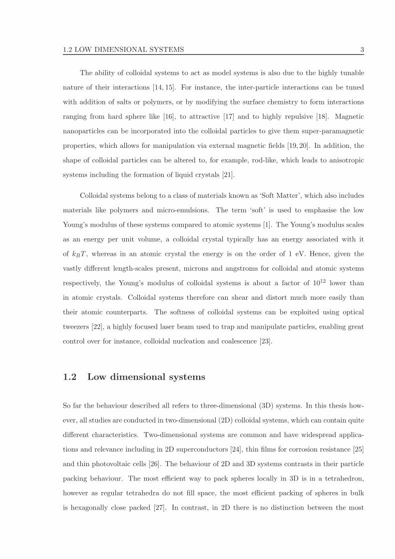
1.2 Low dimensional systems
So far the behaviour described all refers to three-dimensional (3D) systems. In this thesis how-
ever, all studies are conducted in two-dimensional (2D) colloidal systems, which can contain quite
different characteristics. Two-dimensional systems are common and have widespread applica-
tions and relevance including in 2D superconductors [24], thin films for corrosion resistance [25]
and thin photovoltaic cells [26]. The behaviour of 2D and 3D systems contrasts in their particle
packing behaviour. The most efficient way to pack spheres locally in 3D is in a tetrahedron,
however as regular tetrahedra do not fill space, the most efficient packing of spheres in bulk
is hexagonally close packed [27]. In contrast, in 2D there is no distinction between the most
4 GENERAL INTRODUCTION
efficient local and long range packing behaviour, spheres in a 2D plane pack most efficiently
hexagonally.
The melting transition is a very notable example of how behaviour is greatly influenced by
dimensionality [28]. In contrast to 3D crystals which melt via a first order phase transition, in
2D, crystals melt via a two step scenario with an intermediate hexatic phase, characterised by
quasi-long range orientational and short range translational order [18]. Interfaces can also be
considered to be a form of a low dimensional system, for instance the particles constituting a
grain boundary, which is the interface between two crystallites. For a 1D interface in a 2D crystal
the interfacial tension scales as the inverse of the particle diameter, therefore colloidal systems
have a far lower interfacial tension than atomic and molecular systems [14]. Consequently, the
interface fluctuations in colloidal systems due to thermal energy are more significant and more
easily observed [29].
1.3 Scope of this thesis
In this thesis the behaviour of 2D colloidal systems is investigated using optical video microscopy,
optical tweezing and external magnetic fields. These tools enable the study of grain boundaries
and other forms of confinement in 2D colloidal systems.
The chapters are organised as follows. Firstly, in chapter 2, the colloidal model systems
and the experimental techniques and background are introduced. This includes the various
properties of the colloidal particles used and the set-up and design of the optical tweezer and
optical microscope. The Helmholtz coils for generating magnetic fields and sample cell design
and manufacture are described before the image capture and image processing are introduced.
Grain boundary fluctuations in 2D colloidal crystals are described in chapter 3. Grain
boundaries define material strength, but as experimentally studying atomic grain boundaries is
difficult, previous studies on grain boundary fluctuations have focused on simulations. In this
experimental work, the grain boundary study utilises and builds upon the analytical techniques
used in molecular dynamics computer simulations [30], not only to probe the behaviour of
colloidal grain boundaries directly, but to act as an experimental test for interface fluctuation

1.3 SCOPE OF THIS THESIS 5
theories. The fluctuations of a grain boundary in a 2D colloidal crystal were analysed and the
grain boundary properties determined via several complimentary methods derived from capillary
wave theory.
In chapter 4, the dynamics of the colloidal particles constituting a grain boundary in a
2D colloidal crystal are analysed. It has long been hypothesised that the dynamics of grain
boundary particles may show dynamics similar to supercooled liquids [31]. This hypothesis was
corroborated recently by molecular dynamics simulations [32]. The aim of this chapter is to test
this long standing hypothesis in experiment. The dynamics of the grain boundary particles are
shown to be highly heterogeneous, with non-Gaussian distributions and to contain co-operatively
rearranging regions, all behaviour characteristic of supercooled systems.
The most efficient packing of spherical particles in 2D is hexagonally. In chapter 5, the
packing of spherical particles into pentagonal confinement is investigated. Using an optical
tweezer, colloidal particles are fixed into position creating a pentagon, within which further
particles are confined. The state of the system depends on both the interaction potential and
the number density. Firstly, the effect of lowering the inter-particle interactions via an external
magnetic field is assessed. Secondly, the packing frustration and the consequences for the orien-
tational and dynamical behaviour are analysed when the number of confined colloidal particles
is sequentially increased. Partially melting from a crystal-like to a confined liquid-like state was
observed when the particle interaction potential was deceased. In contrast, re-entrant orienta-
tional particle ordering and fluctuating levels of particle movement were observed as the number
density of the confined particles was increased.
In chapter 6 the question of how the dynamics of fluids are affected in random confinement
is addressed. Transport of fluids in random porous media has important consequences for fields
as diverse as filtration and catalysis [33]. A 2D system is created where small colloidal particles
(the fluid) are free to move within a randomly distributed array of large particles fixed in
position (the matrix). The effective area fraction of the fluid and the matrix particles are
controlled via the inter-particle interaction potential and the number density. State points
along lines across a state diagram of the effective area fraction of the fluid to that of the matrix

6 GENERAL INTRODUCTION
are analysed. Predictions emanating from theory [34] and simulation [35], including from the
Lorentz model [36], are tested in this experimental system at the corresponding regions of the
state diagram. Upon increasing the effective area fraction the dynamics of the fluid particles
are shown to follow a standard glass transition at low matrix density, and a more localisation
dominated glass transition at high matrix density, consistent with both theory and simulation.
Chapter 2
Background and experimental
methods
ABSTRACT
In this thesis colloidal particles are used as a model system for studying a range of condensed
matter phenomena ranging from the dynamics of fluids in confinement to grain boundary fluc-
tuations. As such, colloidal particles and their interactions are relevant to each chapter and
will be introduced here along with the general experimental techniques. The main experimental
set-up is an inverted transmission optical microscope coupled with an infrared optical tweezer
and an array of electromagnets. The theory behind optical tweezing will be briefly described
before the experimental set-up is explained. Lastly, the manufacture and use of sample cells,
image capture and processing, and the particle tracking procedures are introduced.
7
8 BACKGROUND AND EXPERIMENTAL METHODS
2.1 Colloidal particles
2.1.1 Hard spheres
Colloidal particles, as introduced in chapter 1, are micron-sized particles dispersed in a solvent,
e.g. water. The simplest form of colloidal interaction is a hard sphere interaction. The particles
have zero interaction at centre to centre distances greater than the particle diameter and an in-
finitely repulsive interaction potential otherwise. This hard potential results in all phase changes
being purely entropic. Understanding the entropy driven world colloidal hard spheres inhabit is
vital to understanding many phenomena in soft matter. As only excluded volume interactions
exist, the hard sphere phase diagram depends solely upon the particle volume fraction. The
hard sphere volume fraction is represented by φ = ρv, where ρ is the number density and v the
particle volume.
The existence of a fluid-solid phase transition in a purely repulsive system was suggested as
long ago as 1914 by Bridgman [37]. However, it was not until 1957 that conclusive evidence for
a phase transition was given. Computer simulations by Wood and Jacobson [38] and Alder and
Wright [39] demonstrated that at sufficiently high densities hard spheres systems can crystallise.
This disorder-order transition occurs at the point when the configurational entropy of the fluid
state is outweighed by the free volume entropy of the ordered solid. Accurate mapping of
the phase boundaries of the hard sphere phase diagram was then later achieved in 1968 by
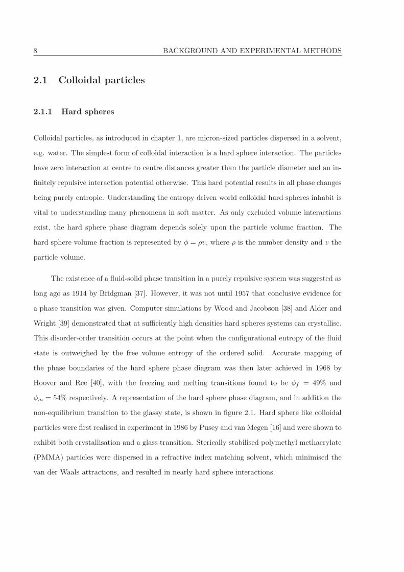
Hoover and Ree [40], with the freezing and melting transitions found to be φf = 49% and
φm = 54% respectively. A representation of the hard sphere phase diagram, and in addition the
non-equilibrium transition to the glassy state, is shown in figure 2.1. Hard sphere like colloidal
particles were first realised in experiment in 1986 by Pusey and van Megen [16] and were shown to
exhibit both crystallisation and a glass transition. Sterically stabilised polymethyl methacrylate
(PMMA) particles were dispersed in a refractive index matching solvent, which minimised the
van der Waals attractions, and resulted in nearly hard sphere interactions.
2.1 COLLOIDAL PARTICLES 9
Fluid
Volume fraction %
54% 74%
58% 64%
Fluid +crystal
Crystal
Glass
49%
Figure 2.1: Hard sphere phase diagram displaying the regions of fluid, crystal, coexistence
and the non-equilibrium glassy state. Note that the illustrations are two dimensional (2D)
representations, the phase transitions are for a three dimensional (3D) system.
2.1.2 Charged spheres
In water based colloidal systems, charges emanating from dissolved ions and surface groups
play a vital role in determining inter-particle interactions. Colloidal particles always experi-
ence attractive van der Waals forces at short distances when dispersed in solvents. Therefore,
without a stabilising repulsive interaction, the particles will aggregate, often irreversibly. Two
solutions to this problem are charge stabilisation and steric stabilisation. The latter involves
adding an adsorbing or grafting polymer to the particle surface. Inter-particle steric repulsion is
created due to entropic effects when polymer chains of neighbouring particles interact. Charge
stabilisation involves modifying the particle surface during synthesis to add dissociating surface
groups. Typically particles are stabilised with carboxyl surface groups, which dissociate in polar
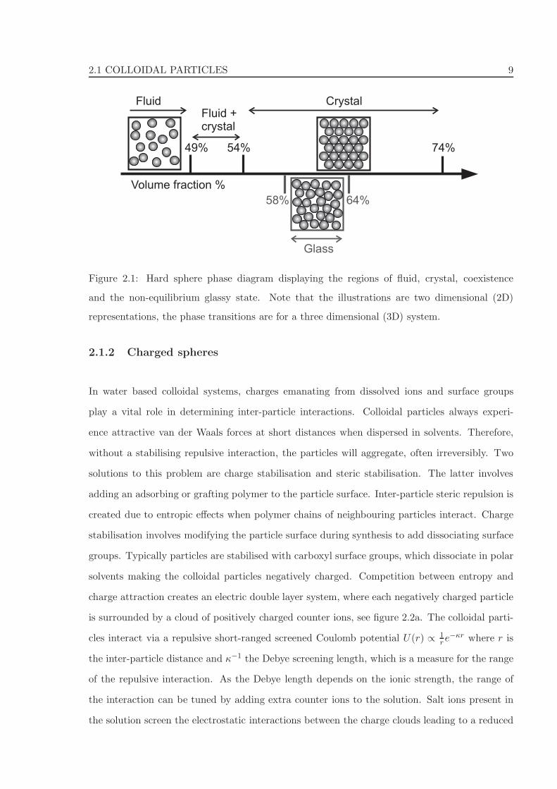
solvents making the colloidal particles negatively charged. Competition between entropy and
charge attraction creates an electric double layer system, where each negatively charged particle
is surrounded by a cloud of positively charged counter ions, see figure 2.2a. The colloidal parti-
cles interact via a repulsive short-ranged screened Coulomb potential U(r) ∝ 1re
−κr where r is
the inter-particle distance and κ−1 the Debye screening length, which is a measure for the range
of the repulsive interaction. As the Debye length depends on the ionic strength, the range of
the interaction can be tuned by adding extra counter ions to the solution. Salt ions present in
the solution screen the electrostatic interactions between the charge clouds leading to a reduced
10 BACKGROUND AND EXPERIMENTAL METHODS
+--
--
-
-
--
- -
- -- -
--
+
+
++
++
++
+ +
++
+
+
++
+
+
++
++ +
+
+
+
+
+
--- - -- -
---+
+
+
++
++
++
+ +
++
+
+
++
+
+
+
+
+
++ +
+
+
+
+
+
+
+--
--
-
-
--
- -
- -- -
--+
++
++
++
+ +
++
+
++
+
+
+
+
+
++ +
+
++
+
++
--- - -- -
---
++
++
++
+
+
+
++
+
++
+ +
++
+
+
+
+
+
+
+
+
+
++ +
+
++
++
+
-
--
- -
-- -
---
--
-
-
--
- -
- -- -
----
- - -- ----
---
-
-
-
--
- -
- -- -
--
- - - ---
-
-
- - -
-
--
--
-
--
-
-
Electrostatic repulsion 0.0 0.2 0.4 0.6 0.8 1.00
5
10
r
U(r)
a b
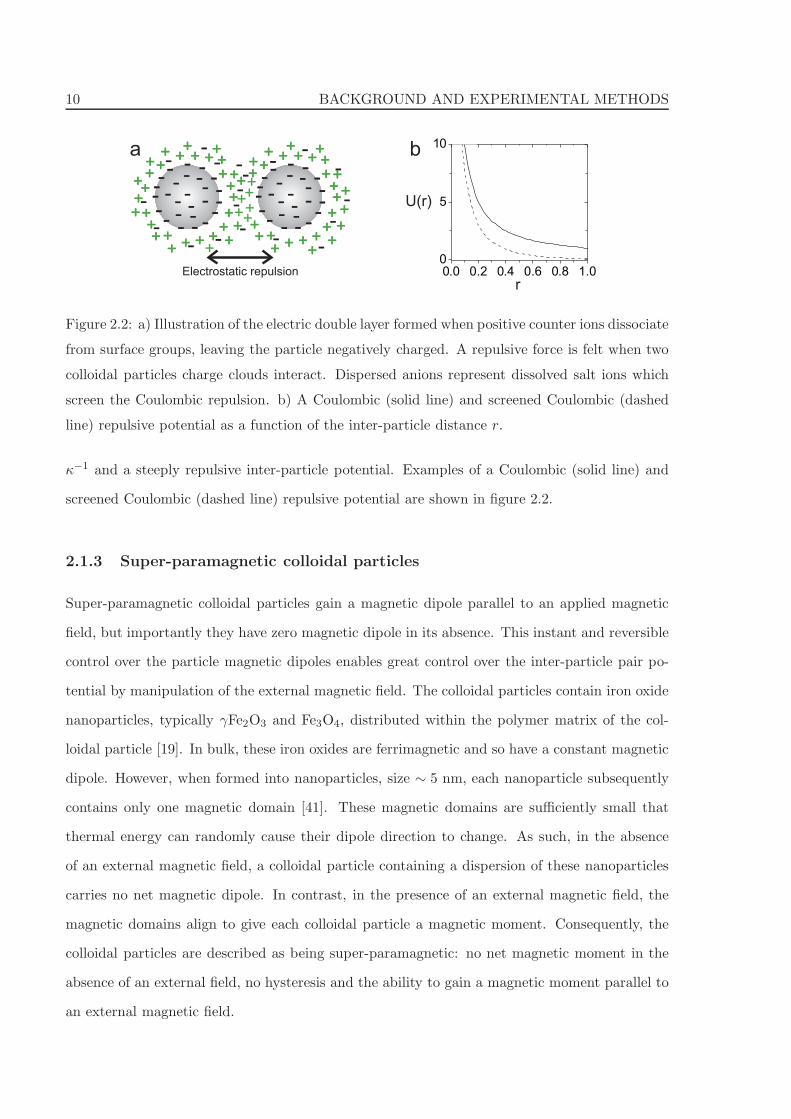
Figure 2.2: a) Illustration of the electric double layer formed when positive counter ions dissociate
from surface groups, leaving the particle negatively charged. A repulsive force is felt when two
colloidal particles charge clouds interact. Dispersed anions represent dissolved salt ions which
screen the Coulombic repulsion. b) A Coulombic (solid line) and screened Coulombic (dashed
line) repulsive potential as a function of the inter-particle distance r.
κ−1 and a steeply repulsive inter-particle potential. Examples of a Coulombic (solid line) and
screened Coulombic (dashed line) repulsive potential are shown in figure 2.2.
2.1.3 Super-paramagnetic colloidal particles
Super-paramagnetic colloidal particles gain a magnetic dipole parallel to an applied magnetic
field, but importantly they have zero magnetic dipole in its absence. This instant and reversible
control over the particle magnetic dipoles enables great control over the inter-particle pair po-
tential by manipulation of the external magnetic field. The colloidal particles contain iron oxide
nanoparticles, typically γFe2O3 and Fe3O4, distributed within the polymer matrix of the col-
loidal particle [19]. In bulk, these iron oxides are ferrimagnetic and so have a constant magnetic
dipole. However, when formed into nanoparticles, size ∼ 5 nm, each nanoparticle subsequently
contains only one magnetic domain [41]. These magnetic domains are sufficiently small that
thermal energy can randomly cause their dipole direction to change. As such, in the absence
of an external magnetic field, a colloidal particle containing a dispersion of these nanoparticles
carries no net magnetic dipole. In contrast, in the presence of an external magnetic field, the
magnetic domains align to give each colloidal particle a magnetic moment. Consequently, the
colloidal particles are described as being super-paramagnetic: no net magnetic moment in the
absence of an external field, no hysteresis and the ability to gain a magnetic moment parallel to
an external magnetic field.
2.1 COLLOIDAL PARTICLES 11
When in the presence of an external magnetic field, the super-paramagnetic colloidal par-
ticles can be approximated to point dipoles as the iron oxide nanoparticle density is fairly
homogeneous (for a typical example see [19]). An external magnetic field, ~B, induces in particle
1, a dipole moment ~m1 in the direction of ~B. At low external magnetic fields the magnitude,
m, of the induced magnetic moment, ~m1, is proportional to the applied field, m = χB, where χ
is the magnetic susceptibility, a material specific property. The magnetic field induced, ~B1(~r),
by the point dipole of particle 1 at the position of particle 2, a distance r away is [42]:
~B1(~r) =µ0
4π
1
r3[3(~m1 · r)r − ~m1] (2.1)
where r is the unit vector between the two dipoles and µ0 is the permeability of free space. The
interaction energy, E, between two dipoles depends on the local magnetic field and the magnetic
moment of the dipole [42]:
E = −~m1~B2 = −~m2
~B1. (2.2)
Substituting eq. (2.1) into eq. (2.2) gives the interaction energy between 2 dipoles in any orien-
tation connected by vector ~r as:
E12(~r) =µ0
4π
1
r3[~m1 · ~m2 − 3(~m1 · r)(~m2 · r)]. (2.3)
The applied field is homogeneous in strength so all induced dipoles must have equal magnitude
moments, m, parallel to the field. By expanding r = 1r · ~r the expression can be simplified to:
E12(~r) =µ0
4π
1
r5[m2r2 − 3(~m · ~r)2]. (2.4)
As all systems in this thesis are 2D, with the external magnetic field perpendicular to the plane,
~m and ~r are always orthogonal, and therefore:
E12(r) =µ0
4π
m2
r3=
µ0
4π
χ2B2
r3. (2.5)
This expression then yields the repulsive interaction energy of two induced dipoles in a plane
perpendicular to the external magnetic field.
12 BACKGROUND AND EXPERIMENTAL METHODS
2.1.4 Brownian motion
As alluded to in chapter 1, it is Brownian motion that is the key behind why colloidal systems
are so rich in phenomenology and so useful as ‘model atoms’. The constant bombardment of
the colloidal particles by the solvent molecules gives the colloidal particles the thermal energy to
explore phase space. Einstein, and separately Sutherland, described how Brownian motion can
be related to a particle’s diffusion coefficient, D [9,43]. It should be noted that all the relations
given here regarding Brownian motion relate to a system at infinite dilution. The diffusion
coefficient, D, of a particle undergoing Brownian motion is given by:
D =kBT
ζ=
kBT
6πηR(2.6)
where the latter is known as the Stokes-Einstein equation, the denominator is the Stokes relation,
kB the Boltzmann factor and T the temperature. The Stokes relation, ζ = 6πηR, relates the
friction factor, ζ, to the radius, R, of a spherical particle moving through a solvent of viscosity,
η. To quantify the effect of Brownian motion on the colloidal particles and find an intrinsic
timescale, the Brownian time is introduced and defined as the time taken for a particle to
diffuse over its own diameter. The Brownian time in 2D, is derived from the mean square
displacement, 〈r2(t)〉 = 4Dt. Setting the particle displacement, r, equal to the particle diameter
gives the Brownian time as τ = R2
D . For a 1 µm particle this gives a Brownian time of ∼ 1 s. The
time and length-scales associated with colloidal particles allow standard optical video microscopy
to be used to observe the colloidal particles in real time. Contrast this to the typical time and
length-scales of atomic systems, where the atoms are ∼ 0.1 nm and the ‘Brownian times’ ∼ 1 ps,
and the clear advantages of colloidal systems as a study medium for many phenomena, and as
atomic models become apparent.
The basic colloidal system where polymer spheres dispersed in water are stabilised by
screened Coulombic repulsions has been described. All experiments in this thesis are concerned
with 2D systems where the particles are sedimented into a plane, therefore the particles must
be more dense than the surrounding medium. The gravitational height, hg, the height at which

2.1 COLLOIDAL PARTICLES 13
a particle attains kBT of gravitational energy, is given by:
hg =3kBT
4πR3g∆ρ(2.7)
where R is the particle radius, ∆ρ the particle-solvent mass density difference and g the accel-
eration due to gravity. To create a 2D system and neglect gravitational effects, a gravitational
height much smaller than the particle is required.
2.1.5 Experimental colloidal systems
Melamine formaldehyde colloidal particles
The melamine formaldehyde colloidal particles used in this work have a diameter of 2.7 µm and
a high cross-linking density, making their structure extremely stable to temperature, acidity
and solvent changes (microParticles). These colloidal particles are used in chapters 3 and 4
on colloidal grain boundaries. They are highly spherical and have good monodispersity with
a coefficient of variation of < 3%. The polymer spheres have a surface layer of carboxylic
acid groups. This gives the particles a hydrophilic anionic surface charge when dispersed in
water, leading to soft screened Coulombic repulsions and prevention of particle aggregation.
The melamine particles have a mass density of 1.5 gcm−3 and refractive index of 1.68. This
leads to good optical tweezing properties and a gravitational height of 0.08 µm, thus enabling
the minimal, out of the plane thermal fluctuations to be neglected. The Brownian time of these
particles at infinite dilution is 11 s, hence their dynamics are sufficiently slow that they can
easily be studied in real time.
Super-paramagnetic colloidal particles
Within this work, three different sizes of super-paramagnetic colloidal particles are used. The
2.8 µm diameter Dynabeads M-270 colloidal particles are used in chapter 5. These are highly
monodisperse cross-linked polystyrene spheres with a < 3% coefficient of variation. The carboxyl
surface groups give the particles a slight negative charge preventing the need for stabilising
surfactants. The particles contain γFe2O3 and Fe3O4 nanoparticles evenly dispersed in the
polymer matrix. This homogeneous distribution allows the particles to be treated as point

14 BACKGROUND AND EXPERIMENTAL METHODS
dipoles when in the presence of an external magnetic field. The colloidal particles have a
Brownian time of 13 s and a gravitational height of 0.07 µm.
In chapter 6, two sizes of particles are used, 3.9 µm (S2180) and 4.95 µm (S2490) in
diameter (microParticles). These super-paramagnetic spheres are also cross-linked polystyrene
particles containing a dispersion of iron oxide nanoparticles (γFe2O3 and Fe3O4), and are charge
stabilised in water. The refractive index is 1.6 and the density ∼ 1.7 gcm−3 and ∼ 1.6 gcm−3
for the 3.9 µm and 4.95 µm diameter particles respectively. The gravitational heights for the
small and large particles are both sufficiently small that gravitational effects can be neglected
(0.02 µm and 0.01 µm respectively). The typical Brownian times for these particles are about
34 s (small) and 70 s (large) at infinite dilution.
As mentioned in section 2.1.3, at low external magnetic fields (up to ∼ 20 mT) the induced
magnetic moment, m, is directly proportional to the applied field B. The proportionality factor,
χ, is the effective magnetic susceptibility where m = χB. The interaction energy between two
super-paramagnetic particles, 1 and 2, positioned in a 2D plane, acting as induced dipoles in an
orthogonally directed external magnetic field is given by eq. (2.5), E12(r) = µ0χ2B2/4πr3. To
be able to map the magnetic inter-particle interactions as a function of B, it is first important
to know the magnetic susceptibility as the interaction potential scales as χ2.
A SQUID (super conducting quantum interference device) is used to measure very weak
magnetic fields and can be used to find the magnetic susceptibility χ [44]. The magnetisation
curves measured by a SQUID magnetometer are shown in figure 2.3. These show the magnetic
moment induced, per colloidal particle, as a function of the applied magnetic field. The probing
magnetic field is taken up from 0 T via the two extremities in magnetic field and finally back up
to the highest magnetic field again. The shape of the magnetic moment response is characteristic
of super-paramagnetic particles. There is negligible hysteresis, a linear response regime at low
applied magnetic field and a saturation at higher magnetic fields (where not shown, the plateau
is at ∼ 0.5 T). The full magnetisation curve, figure 2.3, can be represented by a Langevin
equation:
m(B)
m0= coth(αB)− 1/αB (2.8)

2.2 OPTICAL TWEEZING AND MICROSCOPY 15
-0.2 -0.1 0.0 0.1 0.2
-0.8
-0.4
0.0
0.4
0.8
m(1
0-1
2A
m2)
B (T)
Figure 2.3: Magnetisation curve for super-paramagnetic colloidal particles of diameter 2.8 µm
(dashes), 3.9 µm (solid) and 4.95 µm (dash dot), normalised per particle. All three particle sets
show negligible hysteresis (probing field path 0 T → max T → - max T → max T).
where coth is the hyperbolic tangent, m0 the saturation magnetisation and α a fitting parameter
[20]. Expanding the right hand side as a first order Taylor series gives:
m(B) ≃m0αB
3= χB (2.9)
where χ = m0α/3. Using the approximation eq. (2.9) and m0 and α found from Langevin fits
to the magnetisation curves in figure 2.3, the magnetic susceptibility χ is found.
Particle type Diameter µm χ 10−12Am2T−1
Dynabeads Polystyrene M-270 2.7 6.7
microParticles Polystyrene PS-MAG-S2180 3.9 6.4
microParticles Polystyrene PS-MAG-COOH-S2490 4.95 9.3
2.2 Optical tweezing and microscopy
2.2.1 Optical microscopy
Optical microscopy is used throughout this thesis to study 2D colloidal systems. The oldest
known form of optical microscope is that produced around 1600 when two lenses were mounted
16 BACKGROUND AND EXPERIMENTAL METHODS
Light source
Condensing lens
Sample cell
Sample stage
Imaging objective
Camera
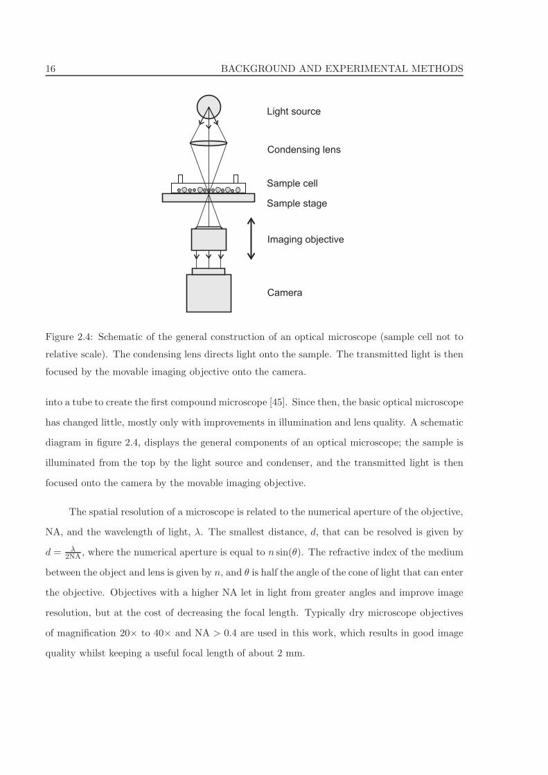
Figure 2.4: Schematic of the general construction of an optical microscope (sample cell not to
relative scale). The condensing lens directs light onto the sample. The transmitted light is then
focused by the movable imaging objective onto the camera.
into a tube to create the first compound microscope [45]. Since then, the basic optical microscope
has changed little, mostly only with improvements in illumination and lens quality. A schematic
diagram in figure 2.4, displays the general components of an optical microscope; the sample is
illuminated from the top by the light source and condenser, and the transmitted light is then
focused onto the camera by the movable imaging objective.
The spatial resolution of a microscope is related to the numerical aperture of the objective,
NA, and the wavelength of light, λ. The smallest distance, d, that can be resolved is given by
d = λ2NA , where the numerical aperture is equal to n sin(θ). The refractive index of the medium
between the object and lens is given by n, and θ is half the angle of the cone of light that can enter
the objective. Objectives with a higher NA let in light from greater angles and improve image
resolution, but at the cost of decreasing the focal length. Typically dry microscope objectives
of magnification 20× to 40× and NA > 0.4 are used in this work, which results in good image
quality whilst keeping a useful focal length of about 2 mm.
2.2 OPTICAL TWEEZING AND MICROSCOPY 17
2.2.2 Optical tweezers: a brief history
An optical tweezer is a focused beam of light with which particles of size comparable to the
wavelength of light can be manipulated. The ability of light to exert a force on micron-sized
particles was first demonstrated by Arthur Ashkin in 1970 [46]. Ashkin demonstrated how a
weakly focused laser beam could draw objects which had a greater refractive index than the
surrounding medium, towards the beam centre. The objects were also propelled along the
direction of light by the radiation pressure of the laser. Using gravity to balance the laser
radiation pressure he then demonstrated how particles could be trapped and moved by the laser
beam in an inverted geometry [47]. The first single beam gradient force optical trap was created
by Ashkin and co-workers in 1986 [48], where a highly focused laser beam gave the ability to
trap a particle in three dimensions.
The importance and usefulness of optical tweezers was first recognised in biology to trap
cells and viruses [49]. Nowadays, optical tweezers are an important non-invasive technique for
trapping and manipulating objects in a wide range of disciplines from biology to physics [50–53].
In colloidal science their uses range from measuring particle interactions to defect creation in
‘colloidal crystal engineering’ [22,54–58].
2.2.3 Optical tweezer theory
A single beam gradient-force optical tweezer is created by focusing a laser beam through a high
numerical aperture objective lens. A potential energy well is created in 3D by the strong light
gradient around the focal point. A particle with a refractive index greater than the surrounding
medium can be trapped in this diffraction-limited spot. If there is no difference in refractive
index then the particle feels no force.
There are three regimes and theories behind the physics of optical trapping, selected ac-
cording to the ratio of the particle radius, R, to the wavelength of the laser forming the optical
trap, λ. The Rayleigh regime applies where R ≪ λ, the Mie regime where R ∼ λ and the ray
optics regime where R ≫ λ. In the Rayleigh [59] and ray optics regimes, the physics behind
the optical trapping can be explained by decomposition of the total force on the particle into
18 BACKGROUND AND EXPERIMENTAL METHODS
Intensity profile
highlow
Flow
Fgrad
Fhigh
1064nm Laser
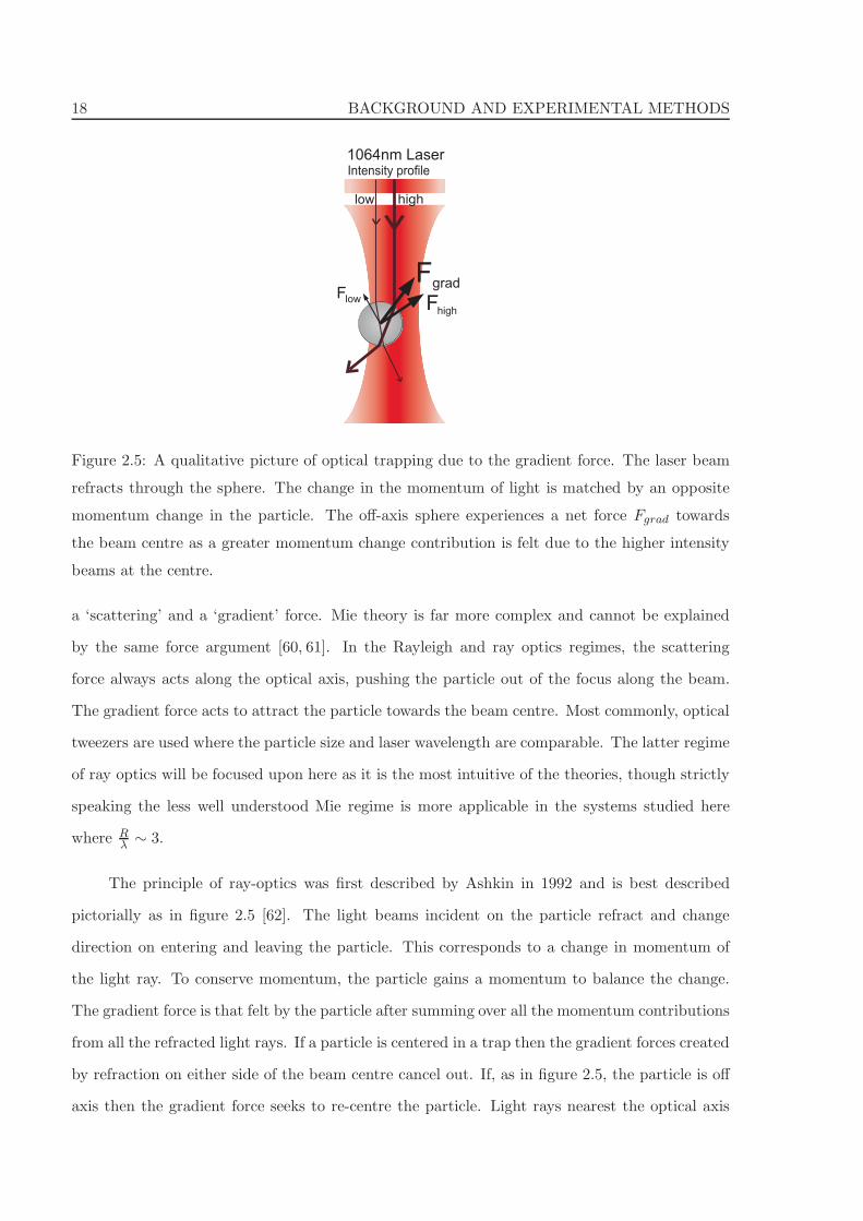
Figure 2.5: A qualitative picture of optical trapping due to the gradient force. The laser beam
refracts through the sphere. The change in the momentum of light is matched by an opposite
momentum change in the particle. The off-axis sphere experiences a net force Fgrad towards
the beam centre as a greater momentum change contribution is felt due to the higher intensity
beams at the centre.
a ‘scattering’ and a ‘gradient’ force. Mie theory is far more complex and cannot be explained
by the same force argument [60, 61]. In the Rayleigh and ray optics regimes, the scattering
force always acts along the optical axis, pushing the particle out of the focus along the beam.
The gradient force acts to attract the particle towards the beam centre. Most commonly, optical
tweezers are used where the particle size and laser wavelength are comparable. The latter regime
of ray optics will be focused upon here as it is the most intuitive of the theories, though strictly
speaking the less well understood Mie regime is more applicable in the systems studied here
where Rλ ∼ 3.
The principle of ray-optics was first described by Ashkin in 1992 and is best described
pictorially as in figure 2.5 [62]. The light beams incident on the particle refract and change
direction on entering and leaving the particle. This corresponds to a change in momentum of
the light ray. To conserve momentum, the particle gains a momentum to balance the change.
The gradient force is that felt by the particle after summing over all the momentum contributions
from all the refracted light rays. If a particle is centered in a trap then the gradient forces created
by refraction on either side of the beam centre cancel out. If, as in figure 2.5, the particle is off
axis then the gradient force seeks to re-centre the particle. Light rays nearest the optical axis
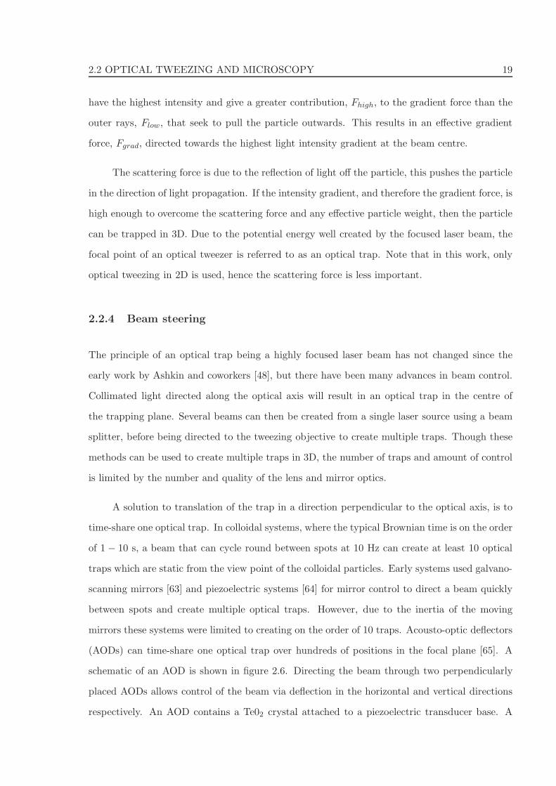
2.2 OPTICAL TWEEZING AND MICROSCOPY 19
have the highest intensity and give a greater contribution, Fhigh, to the gradient force than the
outer rays, Flow, that seek to pull the particle outwards. This results in an effective gradient
force, Fgrad, directed towards the highest light intensity gradient at the beam centre.
The scattering force is due to the reflection of light off the particle, this pushes the particle
in the direction of light propagation. If the intensity gradient, and therefore the gradient force, is
high enough to overcome the scattering force and any effective particle weight, then the particle
can be trapped in 3D. Due to the potential energy well created by the focused laser beam, the
focal point of an optical tweezer is referred to as an optical trap. Note that in this work, only
optical tweezing in 2D is used, hence the scattering force is less important.
2.2.4 Beam steering
The principle of an optical trap being a highly focused laser beam has not changed since the
early work by Ashkin and coworkers [48], but there have been many advances in beam control.
Collimated light directed along the optical axis will result in an optical trap in the centre of
the trapping plane. Several beams can then be created from a single laser source using a beam
splitter, before being directed to the tweezing objective to create multiple traps. Though these
methods can be used to create multiple traps in 3D, the number of traps and amount of control
is limited by the number and quality of the lens and mirror optics.
A solution to translation of the trap in a direction perpendicular to the optical axis, is to
time-share one optical trap. In colloidal systems, where the typical Brownian time is on the order
of 1 − 10 s, a beam that can cycle round between spots at 10 Hz can create at least 10 optical
traps which are static from the view point of the colloidal particles. Early systems used galvano-
scanning mirrors [63] and piezoelectric systems [64] for mirror control to direct a beam quickly
between spots and create multiple optical traps. However, due to the inertia of the moving
mirrors these systems were limited to creating on the order of 10 traps. Acousto-optic deflectors
(AODs) can time-share one optical trap over hundreds of positions in the focal plane [65]. A
schematic of an AOD is shown in figure 2.6. Directing the beam through two perpendicularly
placed AODs allows control of the beam via deflection in the horizontal and vertical directions
respectively. An AOD contains a Te02 crystal attached to a piezoelectric transducer base. A
20 BACKGROUND AND EXPERIMENTAL METHODS
Aco
usto
ab
so
rbe
r
Tra
nsd
uce
r
Te02
Soundwaves
θ
Diffracted beamTransmitted beam
Incident beam
φ
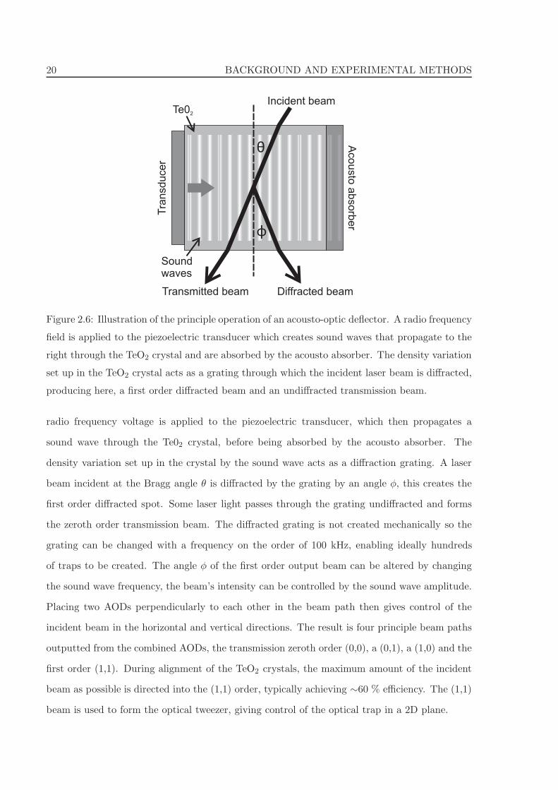
Figure 2.6: Illustration of the principle operation of an acousto-optic deflector. A radio frequency
field is applied to the piezoelectric transducer which creates sound waves that propagate to the
right through the TeO2 crystal and are absorbed by the acousto absorber. The density variation
set up in the TeO2 crystal acts as a grating through which the incident laser beam is diffracted,
producing here, a first order diffracted beam and an undiffracted transmission beam.
radio frequency voltage is applied to the piezoelectric transducer, which then propagates a
sound wave through the Te02 crystal, before being absorbed by the acousto absorber. The
density variation set up in the crystal by the sound wave acts as a diffraction grating. A laser
beam incident at the Bragg angle θ is diffracted by the grating by an angle φ, this creates the
first order diffracted spot. Some laser light passes through the grating undiffracted and forms
the zeroth order transmission beam. The diffracted grating is not created mechanically so the
grating can be changed with a frequency on the order of 100 kHz, enabling ideally hundreds
of traps to be created. The angle φ of the first order output beam can be altered by changing
the sound wave frequency, the beam’s intensity can be controlled by the sound wave amplitude.
Placing two AODs perpendicularly to each other in the beam path then gives control of the
incident beam in the horizontal and vertical directions. The result is four principle beam paths
outputted from the combined AODs, the transmission zeroth order (0,0), a (0,1), a (1,0) and the
first order (1,1). During alignment of the TeO2 crystals, the maximum amount of the incident
beam as possible is directed into the (1,1) order, typically achieving ∼60 % efficiency. The (1,1)
beam is used to form the optical tweezer, giving control of the optical trap in a 2D plane.
2.2 OPTICAL TWEEZING AND MICROSCOPY 21
AODs can only create optical traps in one plane. A Pockels cell can be used with an AOD
to give tweezing in two planes [66], but to create 3D tweezing a different approach is required.
Holographic optical tweezers can create multiple optical traps in 3D arrangements by using
a computer controlled hologram and a spatial light modulator [67–69]. The holograms, and
hence the trap positions can be changed in real time, therefore creating a powerful technique
for multi-object manipulation in fields ranging from nano-technology [70], biology [71, 72] to
microfluidics [73].
2.2.5 Experimental set-up
Two experimental set-ups are used in this work, a stand-alone Olympus inverted bright field
microscope and a custom-built inverted bright field microscope as part of an optical tweezer
set-up. All the microscope designs are inverted to allow observation of colloidal particles from
underneath the sample. A picture of the optical microscope section of the optical tweezer is
shown in figure 2.8, along with a schematic drawing of the whole optical tweezer set-up in
figure 2.7. Here follows a step-by-step guide through the optical tweezer set-up as shown in
figure 2.7. A diode pumped Coherent Compass continuous wave neodymium vanadate laser,
vertically polarised with a wavelength of 1064 nm is used. Firstly, the beam is expanded about
10× in the beam expander, lenses L1 and L2. The vertically polarised laser beam then passes
through the lambda-half plate, W1, and is reflected in the polarising beam splitter, B1. Altering
the beam polarisation with the lambda-half wave plate enables the beam to pass straight through
the beam splitter into a different set-up if required.
The vertically polarised light is directed into first the vertical then the horizontally posi-
tioned AODs, the acousto-optic deflectors (Opto-Electronic), which make up the beam steering
system. In each AOD a sound wave propagating through a TeO2 crystal sets up a standing wave
diffraction grating. This diffraction pattern deflects the laser beam at different angles and inten-
sities according to the sound wave frequency and amplitude respectively. Each AOD diffracts
the incident laser beam into a first order beam and a transmission, zeroth order beam. Careful
alignment of the horizontal and vertical AODs results in ∼ 60% of the laser light being directed
into the (1,1) beam. The mirror, M1, is positioned to only select the (1,1) beam. Any higher
order beams along with the lower order (0,0), (0,1) and (1,0) are directed away. The diffrac-

22 BACKGROUND AND EXPERIMENTAL METHODS
L1 L2 W1
B1
AOD
M1M2
M3M4
L3
L4 W2
L5
Sample
Obj1
B2
F
Camera
Obj2
L
W
B
AOD
M
Lightsource
Obj1
Obj2
F
Lens
Lambda-half wave plate
Polarising beam splitter
Acousto-optic deflector
Mirror
50x 0.55NA Tweezing objective
40x 0.4NA Imaging objective
Infrared band pass filter
LASER
Y
X
Figure 2.7: A schematic of the experimental set-up to create an upright optical tweezer and an
inverted transmission optical microscope.
2.2 OPTICAL TWEEZING AND MICROSCOPY 23
Helmholtz coil
Tweezing objective
Imaging objective
Sample cell
Laser beam
Camera
Beam splitter
Filter
Illumination&
Helmholtz coil
(inside)
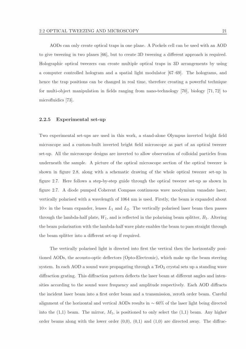
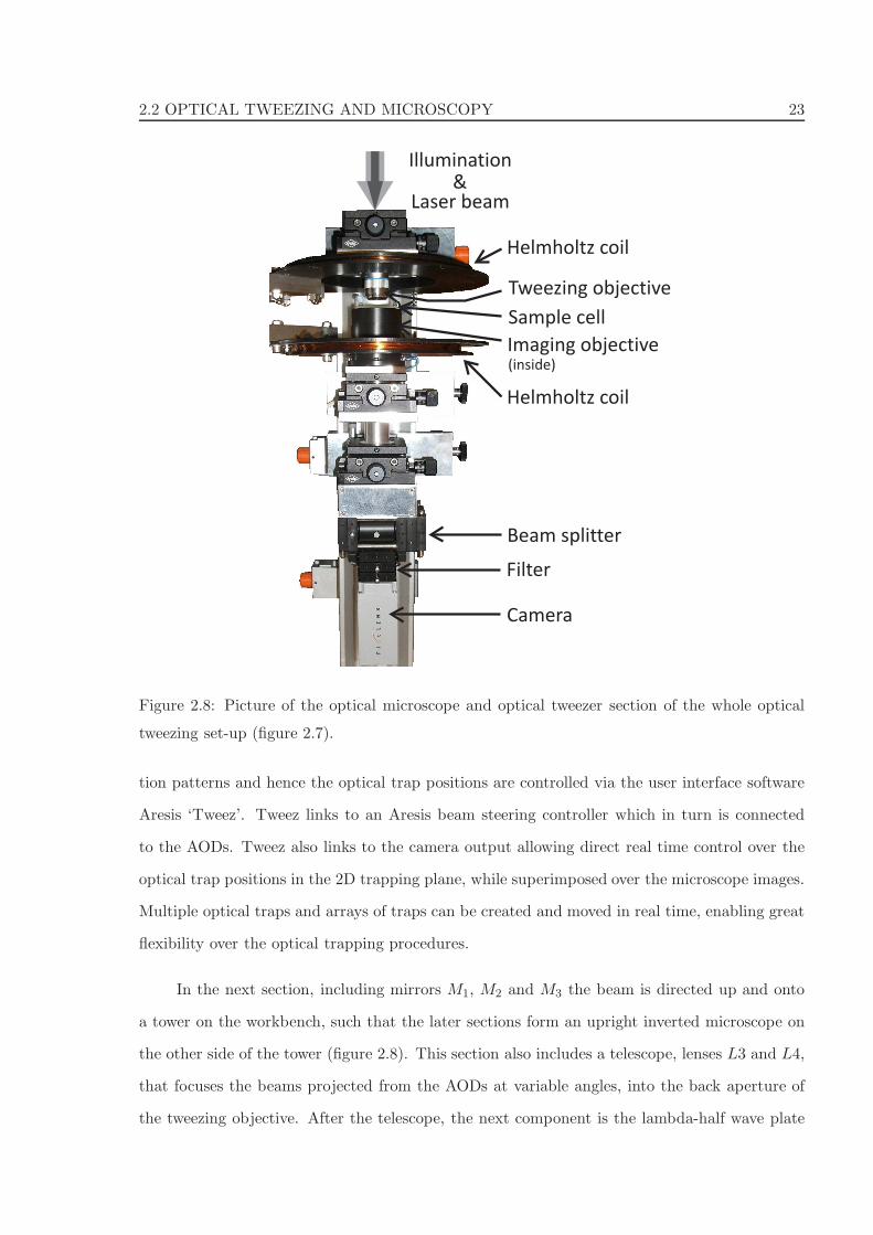
Figure 2.8: Picture of the optical microscope and optical tweezer section of the whole optical
tweezing set-up (figure 2.7).
tion patterns and hence the optical trap positions are controlled via the user interface software
Aresis ‘Tweez’. Tweez links to an Aresis beam steering controller which in turn is connected
to the AODs. Tweez also links to the camera output allowing direct real time control over the
optical trap positions in the 2D trapping plane, while superimposed over the microscope images.
Multiple optical traps and arrays of traps can be created and moved in real time, enabling great
flexibility over the optical trapping procedures.
In the next section, including mirrors M1, M2 and M3 the beam is directed up and onto
a tower on the workbench, such that the later sections form an upright inverted microscope on
the other side of the tower (figure 2.8). This section also includes a telescope, lenses L3 and L4,
that focuses the beams projected from the AODs at variable angles, into the back aperture of
the tweezing objective. After the telescope, the next component is the lambda-half wave plate
24 BACKGROUND AND EXPERIMENTAL METHODS
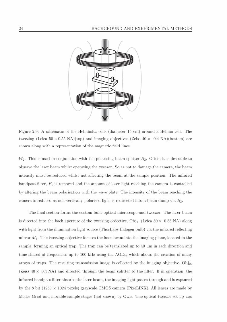
Figure 2.9: A schematic of the Helmholtz coils (diameter 15 cm) around a Hellma cell. The
tweezing (Leica 50× 0.55 NA)(top) and imaging objectives (Zeiss 40 × 0.4 NA)(bottom) are
shown along with a representation of the magnetic field lines.
W2. This is used in conjunction with the polarising beam splitter B2. Often, it is desirable to
observe the laser beam whilst operating the tweezer. So as not to damage the camera, the beam
intensity must be reduced whilst not affecting the beam at the sample position. The infrared
bandpass filter, F , is removed and the amount of laser light reaching the camera is controlled
by altering the beam polarisation with the wave plate. The intensity of the beam reaching the
camera is reduced as non-vertically polarised light is redirected into a beam dump via B2.
The final section forms the custom-built optical microscope and tweezer. The laser beam
is directed into the back aperture of the tweezing objective, Obj1, (Leica 50× 0.55 NA) along
with light from the illumination light source (ThorLabs Halogen bulb) via the infrared reflecting
mirror M4. The tweezing objective focuses the laser beam into the imaging plane, located in the
sample, forming an optical trap. The trap can be translated up to 40 µm in each direction and
time shared at frequencies up to 100 kHz using the AODs, which allows the creation of many
arrays of traps. The resulting transmission image is collected by the imaging objective, Obj2,
(Zeiss 40× 0.4 NA) and directed through the beam splitter to the filter. If in operation, the
infrared bandpass filter absorbs the laser beam, the imaging light passes through and is captured
by the 8 bit (1280 × 1024 pixels) grayscale CMOS camera (PixeLINK). All lenses are made by
Melles Griot and movable sample stages (not shown) by Owis. The optical tweezer set-up was
2.2 OPTICAL TWEEZING AND MICROSCOPY 25
originally designed in Clemens Bechinger’s group at the University of Stuttgart.
The optical tweezer and microscope is also equipped with two Helmholtz coils around the
objectives and sample as shown in figure 2.8 (not shown in figure 2.7). The Helmholtz coils can
generate magnetic fields of up to ± 4 mT perpendicular to the imaging plane, as illustrated in
figure 2.9. The large coil radius with respect to sample size ensures a homogeneous field across
the sample.
The standard Olympus inverted bright-field microscope which forms the additional set-up
is not shown here. This experimental arrangement also has Helmholtz coils to generate magnetic
fields in a similar arrangement to in figure 2.9. This set-up was used solely for microscopy and
used for the work in chapter 6 on ‘Particle dynamics in random confinement’.
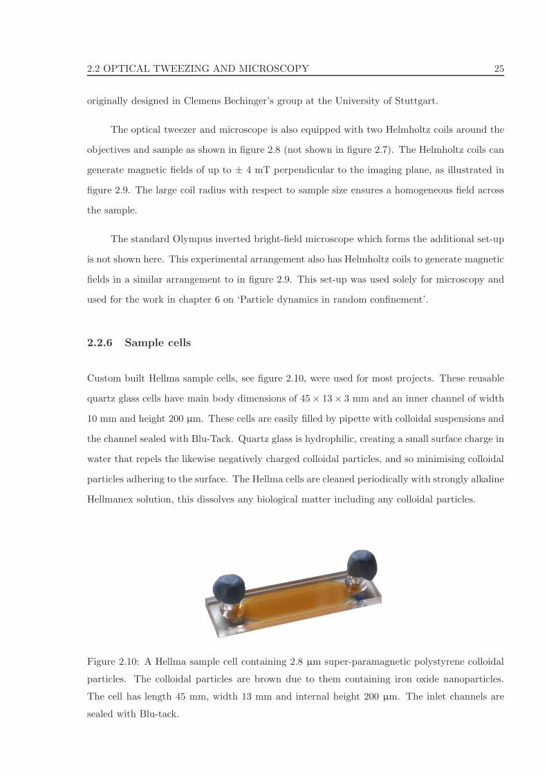
2.2.6 Sample cells
Custom built Hellma sample cells, see figure 2.10, were used for most projects. These reusable
quartz glass cells have main body dimensions of 45× 13× 3 mm and an inner channel of width
10 mm and height 200 µm. These cells are easily filled by pipette with colloidal suspensions and
the channel sealed with Blu-Tack. Quartz glass is hydrophilic, creating a small surface charge in
water that repels the likewise negatively charged colloidal particles, and so minimising colloidal
particles adhering to the surface. The Hellma cells are cleaned periodically with strongly alkaline
Hellmanex solution, this dissolves any biological matter including any colloidal particles.
Figure 2.10: A Hellma sample cell containing 2.8 µm super-paramagnetic polystyrene colloidal
particles. The colloidal particles are brown due to them containing iron oxide nanoparticles.
The cell has length 45 mm, width 13 mm and internal height 200 µm. The inlet channels are
sealed with Blu-tack.
26 BACKGROUND AND EXPERIMENTAL METHODS
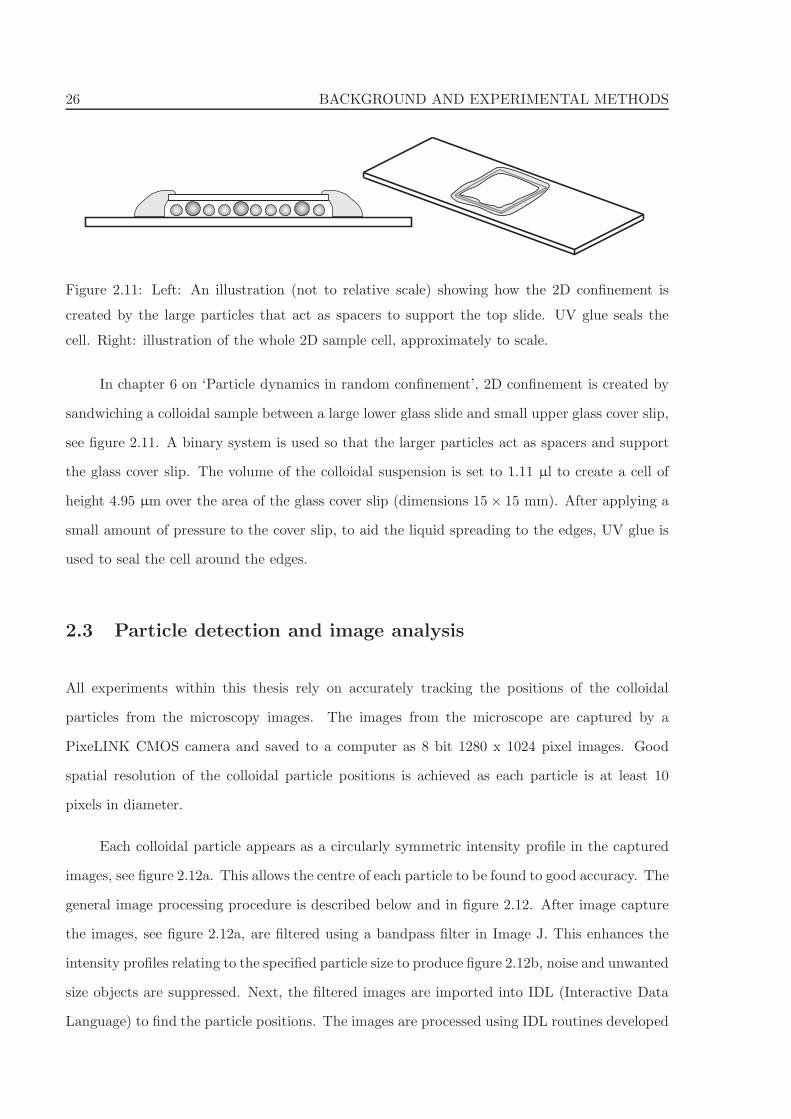
Figure 2.11: Left: An illustration (not to relative scale) showing how the 2D confinement is
created by the large particles that act as spacers to support the top slide. UV glue seals the
cell. Right: illustration of the whole 2D sample cell, approximately to scale.
In chapter 6 on ‘Particle dynamics in random confinement’, 2D confinement is created by
sandwiching a colloidal sample between a large lower glass slide and small upper glass cover slip,
see figure 2.11. A binary system is used so that the larger particles act as spacers and support
the glass cover slip. The volume of the colloidal suspension is set to 1.11 µl to create a cell of
height 4.95 µm over the area of the glass cover slip (dimensions 15× 15 mm). After applying a
small amount of pressure to the cover slip, to aid the liquid spreading to the edges, UV glue is
used to seal the cell around the edges.
2.3 Particle detection and image analysis
All experiments within this thesis rely on accurately tracking the positions of the colloidal
particles from the microscopy images. The images from the microscope are captured by a
PixeLINK CMOS camera and saved to a computer as 8 bit 1280 x 1024 pixel images. Good
spatial resolution of the colloidal particle positions is achieved as each particle is at least 10
pixels in diameter.
Each colloidal particle appears as a circularly symmetric intensity profile in the captured
images, see figure 2.12a. This allows the centre of each particle to be found to good accuracy. The
general image processing procedure is described below and in figure 2.12. After image capture
the images, see figure 2.12a, are filtered using a bandpass filter in Image J. This enhances the
intensity profiles relating to the specified particle size to produce figure 2.12b, noise and unwanted
size objects are suppressed. Next, the filtered images are imported into IDL (Interactive Data
Language) to find the particle positions. The images are processed using IDL routines developed
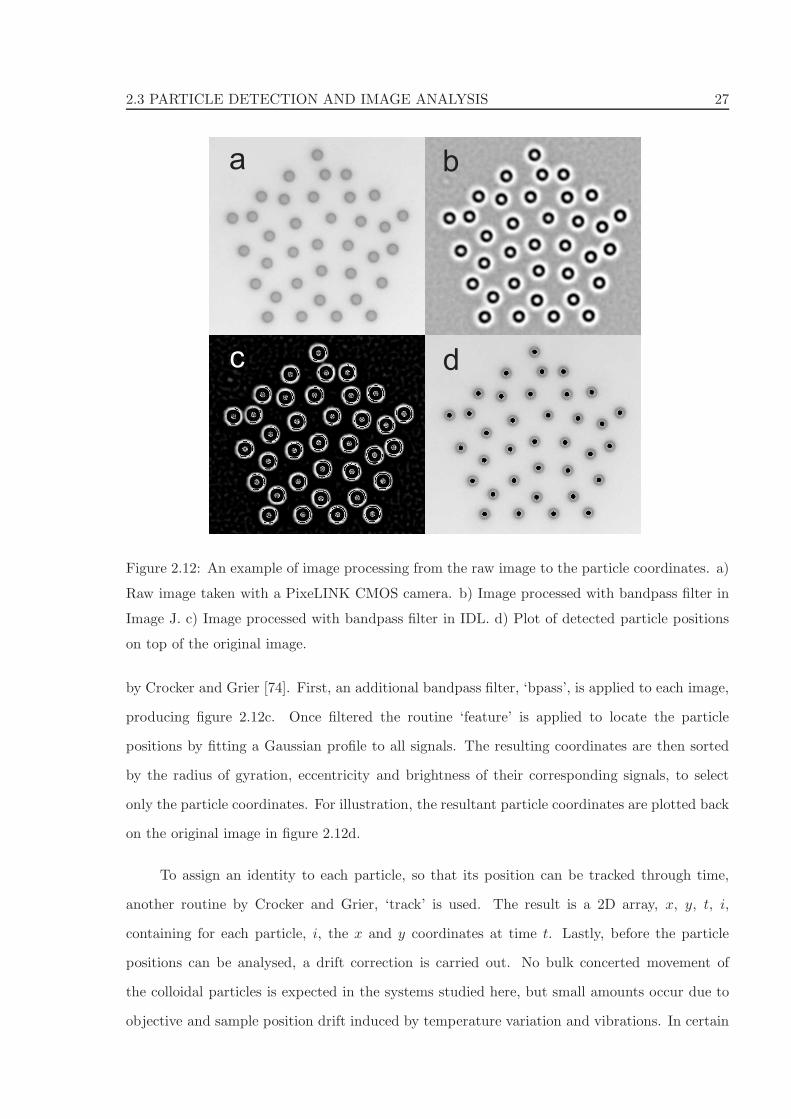
2.3 PARTICLE DETECTION AND IMAGE ANALYSIS 27
a b
c d
Figure 2.12: An example of image processing from the raw image to the particle coordinates. a)
Raw image taken with a PixeLINK CMOS camera. b) Image processed with bandpass filter in
Image J. c) Image processed with bandpass filter in IDL. d) Plot of detected particle positions
on top of the original image.
by Crocker and Grier [74]. First, an additional bandpass filter, ‘bpass’, is applied to each image,
producing figure 2.12c. Once filtered the routine ‘feature’ is applied to locate the particle
positions by fitting a Gaussian profile to all signals. The resulting coordinates are then sorted
by the radius of gyration, eccentricity and brightness of their corresponding signals, to select
only the particle coordinates. For illustration, the resultant particle coordinates are plotted back
on the original image in figure 2.12d.
To assign an identity to each particle, so that its position can be tracked through time,
another routine by Crocker and Grier, ‘track’ is used. The result is a 2D array, x, y, t, i,
containing for each particle, i, the x and y coordinates at time t. Lastly, before the particle
positions can be analysed, a drift correction is carried out. No bulk concerted movement of
the colloidal particles is expected in the systems studied here, but small amounts occur due to
objective and sample position drift induced by temperature variation and vibrations. In certain
28 BACKGROUND AND EXPERIMENTAL METHODS
projects, for instance the pentagonal confinement chapter, a selection of particles are fixed by
the optical tweezer. In these cases all the particle positions are referenced relative to these static
particles. In the grain boundary work, chapters 3 and 4, the particle positions are referenced to
the bulk crystal away from the interface. The particle coordinate data is now in a form to be
analysed.
Acknowledgments
The Clemens Bechinger group at the University of Stuttgart is thanked for the basic optical
tweezing set-up design and Andrew Bothroyd from the University of Oxford for use and assis-
tance with their SQUID magnetometer.
Chapter 3
Grain boundary fluctuations
in 2D colloidal crystals
ABSTRACT
The fluctuations of grain boundaries are studied in two-dimensional (2D) colloidal crystals using
optical video microscopy. The grain boundary fluctuations are quantified by static and dynamic
correlation functions which are both accurately described by expressions derived from capillary
wave theory. This directly leads to the key parameters that describe the grain boundary, the
interfacial stiffness and interface mobility. These parameters are of central importance to the
phenomenon of curvature driven grain boundary migration. Furthermore, the average grain
boundary position is demonstrated to perform a one-dimensional random walk as suggested by
recent computer simulations [Science 314, 632 (2006)]. The value for the interfacial mobility
inferred from this method is in good agreement with those found from the grain boundary
fluctuations.
This chapter is based on and reprinted with permission from [Thomas O. E. Skinner, Dirk G.
A. L. Aarts and Roel P. A. Dullens, (2010), Grain-boundary fluctuations in two-dimensional
colloidal crystals, Phys. Rev. Lett. 105, 168301]. Copyright (2010) by the American Physical
Society.
29
30 GRAIN BOUNDARY FLUCTUATIONS IN 2D COLLOIDAL CRYSTALS
3.1 Introduction
Material microstructure is characterised by the distribution of defects present throughout a
material’s structure. Even crystalline systems contain many imperfections including dislocations
and grain boundaries. Creation of these defects can arise due to stresses on the crystal or as
a result of freezing-in during crystallisation and grain growth. These microstructural defects,
their frequency and distribution, define the physical properties of many materials including
metals, composites and ceramics [75–77]. More specifically, grain boundaries are important
due to their role in many technological materials including high temperature superconductors
[78], thin films for corrosion and wear resistant coatings [25, 79] and in the emerging field of
graphene research [80]. The size and quantity of different crystallites is notably important
for the material’s mechanical properties, whose material strength is directly related to grain
size [81,82]. The evolution and motion of grain boundaries, and therefore the grain size, heavily
influences processes including phase transformations, grain growth and recrystallisation [77,83].
As such, the key to understanding and controlling these processes is the ability to accurately
describe grain boundary formation and migration.
Much of the current experimental knowledge of grain boundaries stems from detailed high-
resolution transmission electron microscopy studies [84–87], yielding information on bulk grain
boundary migration rates. However, accessing the fluctuations of atomic grain boundaries is
a different matter, and is not yet possible due to the inherent time and length scales present
in atomic systems [88]. Hence, only computer simulations have thus far been able to extract
values for the interfacial properties from atomic grain boundaries [30, 89–94]. In contrast to
atomic systems, the time and length scales associated with colloidal systems means interface
fluctuations are more readily accessible [29, 95]. The ability to experimentally follow particle
movement in real time and their thermodynamic equivalence, enables colloidal particles to act
as model systems for atomic materials [96–99]. In this chapter, a 2D colloidal crystal is used
to directly monitor grain boundary fluctuations in real space. Dynamic and static correlation
functions of the fluctuating interfacial profile, which are well described by capillary wave theory,
directly lead to the key grain boundary properties: the interfacial stiffness and mobility. In
addition, the approach suggested in recent computer simulations [100], of determining the grain
3.2 BACKGROUND 31
boundary mobility from the diffusive motion of the mean interface position is experimentally
confirmed.
3.2 Background
3.2.1 Grain boundaries and material properties
The structure of a polycrystalline material is made up of grains, or crystallites, each having a
different orientation to the next. The interface between adjacent grains is known as the grain
boundary, the only difference across the boundary is the grain orientation. As this work focuses
on grain boundaries in two dimensional (2D) crystals, all further descriptions will apply to
defects in 2D systems. In 2D, a grain boundary is a quasi-1D defect composed of an array of
point defects termed dislocations, see figure 3.1. Each dislocation defect is in turn comprised of
two disclinations. In a hexagonal lattice, see figure 3.1a, the two disclinations that constitute
a dislocation are a 5-fold (positive) and 7-fold (negative) coordinated particle. As evidenced
by the insertion of an extra (gray) line in figure 3.1a, an isolated dislocation is a defect that
primarily affects the translational symmetry of the lattice. A free disclination, for instance an
isolated 5-fold defect, disrupts the orientational order of the crystal. The appearance of first
free dislocations and then free disclinations as temperature is increased, forms the basis of the
KTHNY scenario for the melting of 2D crystals [101–103].
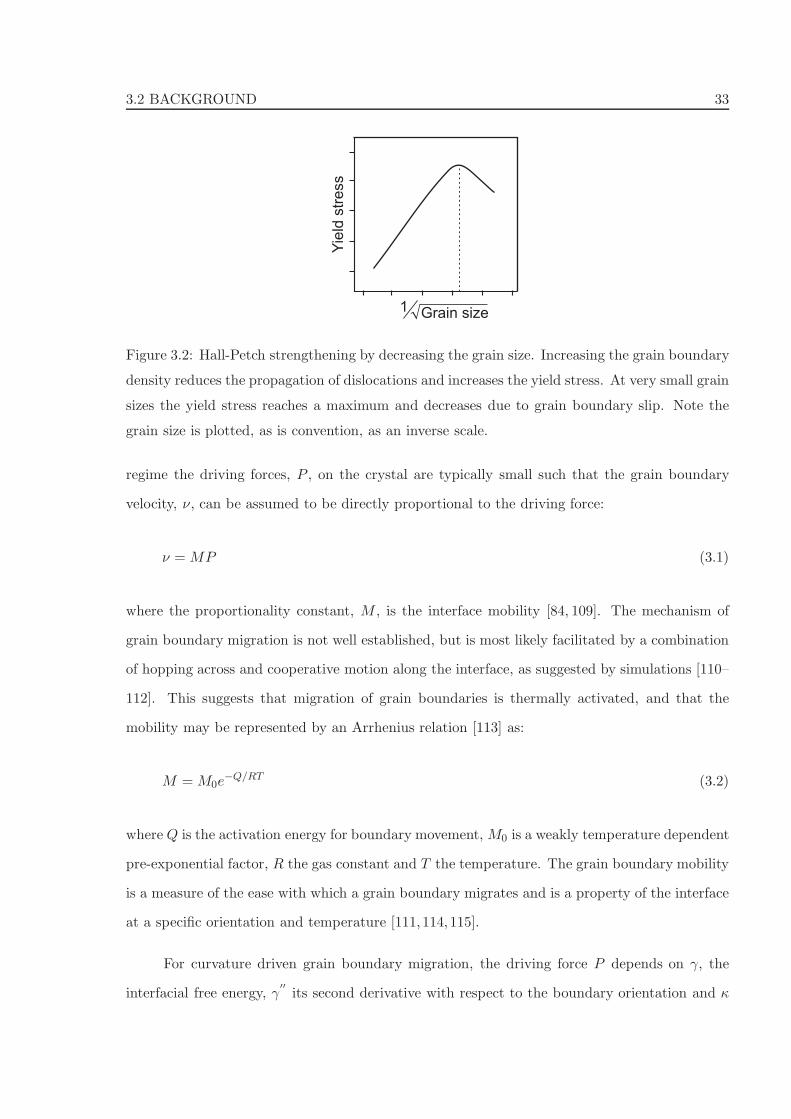
The importance of grain boundaries, in particular their effect on material properties, is
demonstrated by the Hall-Petch law [104–106] which describes the strengthening of materials
by changing the average grain size, see figure 3.2. A measure of material strength is the yield
stress, which is the point at which a material starts fracturing and deforming plastically. The
yield stress of a material is proportional to the resistance to moving dislocations through the
microstructural landscape of defects and grain boundaries. Grain boundaries slow down the
movement of dislocations and resist them traversing grains and propagating the fracture. This
pinning effect stems from two intrinsic properties of grain boundaries; their disordered structure
compared to the crystal and the orientation difference between the crystals, forcing the dislo-
cation to change direction. Hence, increasing the grain boundary density (reducing the grain

32 GRAIN BOUNDARY FLUCTUATIONS IN 2D COLLOIDAL CRYSTALS
- - - ++++-
a b
Figure 3.1: a) An example of an isolated dislocation. The dislocation consists of a 5 and 7-fold
disclination, represented as a positive (+) and a negative (-) coordinated defect respectively.
Vertices correspond to particle positions. The gray lines indicate the effective insertion of an
extra row of particles which disrupts the translational order. b) A chain of dislocations forming
a grain boundary. The gray lines illustrate the change in orientation across the interface.
size) can increase a material’s strength by disrupting this dislocation slip. The Hall-Petch law
states that the yield stress is proportional to the square root of the grain size and therefore as
figure 3.2 illustrates, decreasing the grain size can increase the yield stress. This relationship
applies down to a minimum grain size, after which the structure is so fragmented that grain
boundaries now slide past each other. In this regime, the standard Hall-Petch law no longer
applies, and the yield stress falls with decreasing grain size.
3.2.2 Grain boundary migration
Grain size defines material strength, and grain growth is affected by grain boundary migration,
hence, understanding grain boundary migration is key to controlling grain size. Grain boundaries
naturally migrate through the crystal as both thermal fluctuations and interfacial curvature seek
to shape the interface. Indeed, a polycrystalline structure is not in equilibrium; the grains will
continue to grow until one crystal is formed, albeit very slowly. Other driving forces can emanate
from imbalances or gradients in pressure, defect density or temperature [107, 108]. During
grain growth and recrystallisation an important driving force for microstructure evolution is the
interfacial curvature. This is the drive towards a reduction in the grain boundary surface area,
which competes against the roughening effect of thermal fluctuations. In the curvature driven
3.2 BACKGROUND 33
Grain size
Yie
ld s
tre
ss
√1
Figure 3.2: Hall-Petch strengthening by decreasing the grain size. Increasing the grain boundary
density reduces the propagation of dislocations and increases the yield stress. At very small grain
sizes the yield stress reaches a maximum and decreases due to grain boundary slip. Note the
grain size is plotted, as is convention, as an inverse scale.
regime the driving forces, P , on the crystal are typically small such that the grain boundary
velocity, ν, can be assumed to be directly proportional to the driving force:
ν = MP (3.1)
where the proportionality constant, M , is the interface mobility [84, 109]. The mechanism of
grain boundary migration is not well established, but is most likely facilitated by a combination
of hopping across and cooperative motion along the interface, as suggested by simulations [110–
112]. This suggests that migration of grain boundaries is thermally activated, and that the
mobility may be represented by an Arrhenius relation [113] as:
M = M0e−Q/RT (3.2)
where Q is the activation energy for boundary movement, M0 is a weakly temperature dependent
pre-exponential factor, R the gas constant and T the temperature. The grain boundary mobility
is a measure of the ease with which a grain boundary migrates and is a property of the interface
at a specific orientation and temperature [111,114,115].
For curvature driven grain boundary migration, the driving force P depends on γ, the
interfacial free energy, γ′′
its second derivative with respect to the boundary orientation and κ
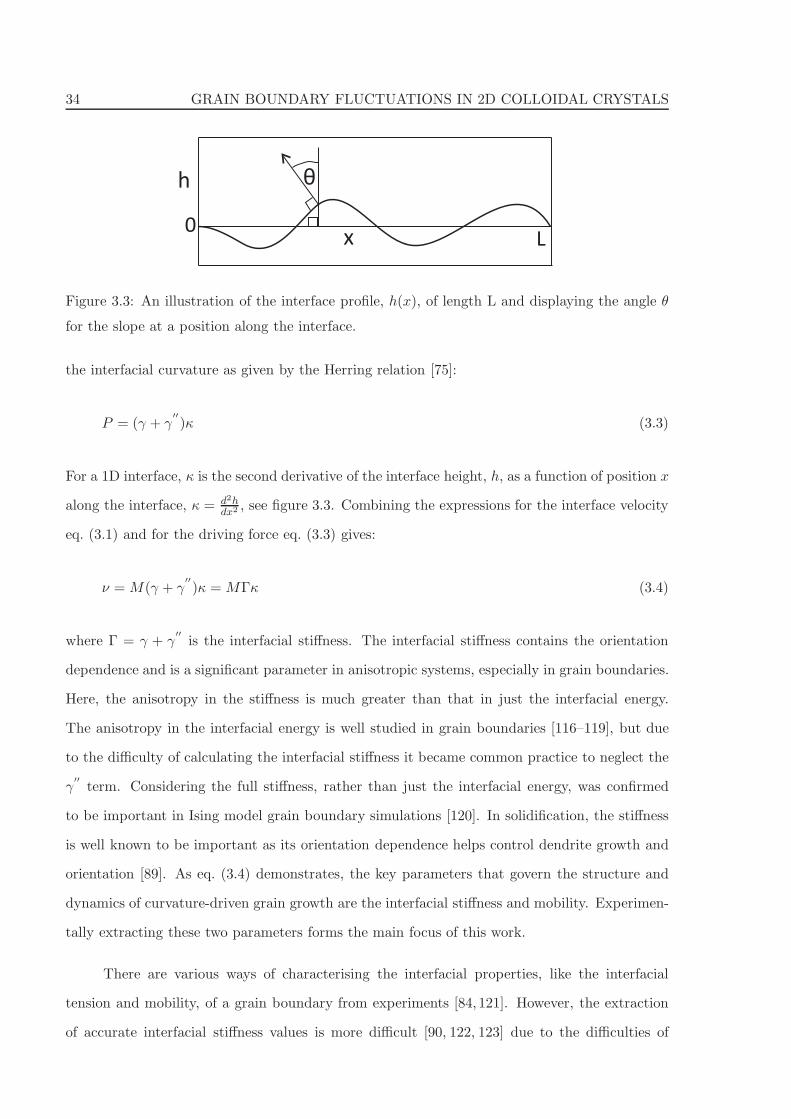
34 GRAIN BOUNDARY FLUCTUATIONS IN 2D COLLOIDAL CRYSTALS
θ
0
h
x L
Figure 3.3: An illustration of the interface profile, h(x), of length L and displaying the angle θ
for the slope at a position along the interface.
the interfacial curvature as given by the Herring relation [75]:
P = (γ + γ′′
)κ (3.3)
For a 1D interface, κ is the second derivative of the interface height, h, as a function of position x
along the interface, κ = d2hdx2 , see figure 3.3. Combining the expressions for the interface velocity
eq. (3.1) and for the driving force eq. (3.3) gives:
ν = M(γ + γ′′
)κ = MΓκ (3.4)
where Γ = γ + γ′′
is the interfacial stiffness. The interfacial stiffness contains the orientation
dependence and is a significant parameter in anisotropic systems, especially in grain boundaries.
Here, the anisotropy in the stiffness is much greater than that in just the interfacial energy.
The anisotropy in the interfacial energy is well studied in grain boundaries [116–119], but due
to the difficulty of calculating the interfacial stiffness it became common practice to neglect the
γ′′
term. Considering the full stiffness, rather than just the interfacial energy, was confirmed
to be important in Ising model grain boundary simulations [120]. In solidification, the stiffness
is well known to be important as its orientation dependence helps control dendrite growth and
orientation [89]. As eq. (3.4) demonstrates, the key parameters that govern the structure and
dynamics of curvature-driven grain growth are the interfacial stiffness and mobility. Experimen-
tally extracting these two parameters forms the main focus of this work.
There are various ways of characterising the interfacial properties, like the interfacial
tension and mobility, of a grain boundary from experiments [84, 121]. However, the extraction
of accurate interfacial stiffness values is more difficult [90, 122, 123] due to the difficulties of
3.2 BACKGROUND 35
controlled experiments on grain boundaries [124]. Therefore, there has been a rapid increase
in the number of grain boundary simulation studies, mostly using molecular dynamics (MD)
[30, 91, 92, 94, 100, 125]. Many of these simulations [30, 90, 91, 100, 126] are based on an elegant
zero-driving force approach where the grain boundary stiffness and mobility are extracted from
the equilibrium grain boundary fluctuations. In this thesis, this analysis of the grain boundary
fluctuations during the curvature driven regime is applied to the grain boundary fluctuations
observed in colloidal experiments.
3.2.3 Capillary wave theory
Grain boundary fluctuations are the sum of thermally excited capillary waves [127–129]. This
forms the basis of the capillary fluctuation method from which the interfacial properties, the
stiffness and mobility, can be determined [30, 89]. The free energy change of disturbing a 1D
interface can be expressed as dE = γ(θ)ds where ds is the change in arc length of the displaced
interface and γ(θ) is the interfacial tension as a function of the angle, θ, between the interface
normal at x and the normal of the flat interface. An illustration of the interface is shown in
figure 3.3. A change in arc length, ds, can be represented via Pythagoras’s theorem as:
ds =
√
1 +dh2
dx2dx (3.5)
where h(x) is the interface height at position x along the interface. The free energy of the whole
interface spanning the system size L can then be written as:
E =
∫ L
0γ(θ)
√
1 + h′(x)2 dx (3.6)
where the prime represents differentiation with respect to x. The anisotropy in γ(θ) can be
expanded to second order in θ:
γ(θ) ≈ γ + γ′
θ +γ
′′
2θ2 (3.7)
where the prime denotes differentiation with respect to θ. Assuming that the interfacial fluctu-
ations are small in amplitude, the arc length can be simplified to:
√
1 + h′(x)2 ≈ 1 +h
′
(x)2
2. (3.8)
36 GRAIN BOUNDARY FLUCTUATIONS IN 2D COLLOIDAL CRYSTALS
and θ can be given in terms of the derivative of h as h′
= dhdx = tan(θ) ≈ θ. Substitution of
eq. (3.7) and eq. (3.8) into eq. (3.6) results in:
E =
∫ L
0
(
γ + γ′
h′
(x) +γ
′′
h′
(x)2
2
)(
1 +h
′
(x)2
2
)
dx. (3.9)
The free energy cannot depend on the sign of the gradient of the function h, therefore, when
multiplying out eq. (3.9), the h′
(x) and h′
(x)3 terms produce no contribution. The term to
fourth order, h′
(x)4, is negligible in size and so the expression becomes:
E =
∫ L
0
(
γ +γh
′
(x)2
2+
γ′′
h′
(x)2
2
)
dx. (3.10)
Integrating out the first term gives Lγ, the free energy of the flat interface. Defining ∆E = E−Lγ
and substituting in the stiffness, where Γ = γ + γ′′
, gives:
∆E =1
2Γ
∫ L
0h
′
(x)2 dx. (3.11)
The interface profile h(x) is expressed as a sum of capillary waves, h(x) =∑
k A(k)eikx, which
after differentiating yields:
h′
(x) =∑
k
ikA(k)eikx (3.12)
where k = n2π/L. Substituting eq. (3.12) into eq. (3.11) gives:
∆E =1
2Γ
∫ L
0
∑
km
ikmA(km)eikmx∑
kn
−iknA∗(kn)e
−iknx dx (3.13)
where A∗(k) is the complex conjugate of A(k). Next, the expression can be simplified by
combining the exponents to give:
∆E =1
2Γ
∫ L
0
∑
km
∑
kn
kmknA(km)A∗(kn)eix(km−kn) dx (3.14)
For the case when km 6= kn, then the argument of the integral is the sum over all wavelengths
and has no contribution. For km = kn, the exponential term collapses to 1 and the expression
simplifies to:
∆E =1
2Γ∑
k
Lk2A(k)A∗(k) (3.15)

3.2 BACKGROUND 37
From the equipartition theorem it follows that each k mode contributes an average energy of
12kBT , so therefore kBT = LΓk2〈|A(k)|2〉, from which the static fluctuation spectrum for a 1D
solid-solid interface is obtained [128,129]:
〈|A(k)|2〉 =kBT
LΓk2(3.16)
where the angular brackets denote a configurational average. This power spectrum forms the
basis of the capillary fluctuation method [30,89–91].
To obtain the dynamic correlation function, Hoyt et al. [30], used a generalised Langevin
equation analysis to determine an expression for the time dependence of the mean square am-
plitude. This corresponds to a dynamic correlation function of the amplitudes of the Fourier
components, A(k):
〈A(k, 0)A∗(k, t)〉 = 〈|A(k)|2〉e−MΓk2t (3.17)
where A∗(k, t) is the complex conjugate and the decay time is τ(k) = 1/(MΓk2). Substituting
the expression for the static capillary fluctuation spectrum, eq. (3.16), for the k2 in the definition
of τ , results in:
〈|A(k)|2〉Lτ−1(k) = MkBT. (3.18)
The interface mobility can thus be extracted via finding τ from the decay of 〈|A(k)|2〉 for each
wavevector.
The remainder of this chapter is organised as follows. Firstly, the experimental methods
and the interface localisation are described. Next, the grain boundary fluctuations are anal-
ysed in terms of first the spatial and then the dynamical correlation functions. In each case, a
real space methodology is derived from the standard Fourier space capillary fluctuation method
before a comparison to the Fourier space method is made. Lastly, in section 3.4.3, the applicabil-
ity is demonstrated, and then the interfacial properties determined, via a fluctuation-dissipation
based real space method developed by Trautt et al. [100].
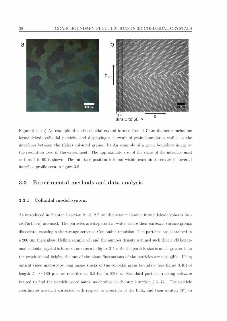
38 GRAIN BOUNDARY FLUCTUATIONS IN 2D COLLOIDAL CRYSTALS
Bins 1 to 60
1234
...
hexp
x
a b
Figure 3.4: (a) An example of a 2D colloidal crystal formed from 2.7 µm diameter melamine
formaldehyde colloidal particles and displaying a network of grain boundaries visible as the
interfaces between the (false) coloured grains. b) An example of a grain boundary image at
the resolution used in the experiment. The approximate size of the slices of the interface used
as bins 1 to 60 is shown. The interface position is found within each bin to create the overall
interface profile seen in figure 3.5.
3.3 Experimental methods and data analysis
3.3.1 Colloidal model system
As introduced in chapter 2 section 2.1.5, 2.7 µm diameter melamine formaldehyde spheres (mi-
croParticles) are used. The particles are dispersed in water where their carboxyl surface groups
dissociate, creating a short-range screened Coulombic repulsion. The particles are contained in
a 200 µm thick glass, Hellma sample cell and the number density is tuned such that a 2D hexag-
onal colloidal crystal is formed, as shown in figure 3.4b. As the particle size is much greater than
the gravitational height, the out of the plane fluctuations of the particles are negligible. Using
optical video microscopy long image stacks of the colloidal grain boundary (see figure 3.4b) of
length L ∼ 180 µm are recorded at 0.5 Hz for 2500 s. Standard particle tracking software
is used to find the particle coordinates, as detailed in chapter 2 section 2.3 [74]. The particle
coordinates are drift corrected with respect to a section of the bulk, and then rotated (4◦) to
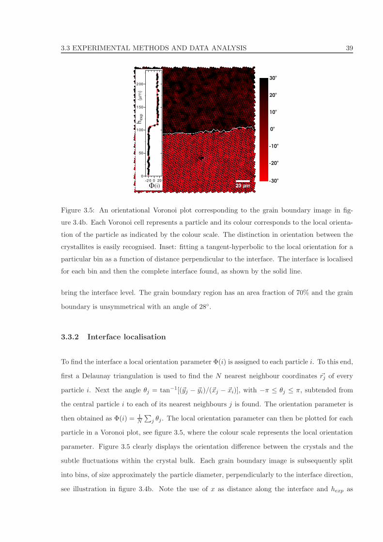
3.3 EXPERIMENTAL METHODS AND DATA ANALYSIS 39
20o
10o
0o
-10o
-20o
-30o
30o
-2 0 0 20
0
50
1 00
1 50
2 00
Φ(i)
he
xp(
m)
μ
Figure 3.5: An orientational Voronoi plot corresponding to the grain boundary image in fig-
ure 3.4b. Each Voronoi cell represents a particle and its colour corresponds to the local orienta-
tion of the particle as indicated by the colour scale. The distinction in orientation between the
crystallites is easily recognised. Inset: fitting a tangent-hyperbolic to the local orientation for a
particular bin as a function of distance perpendicular to the interface. The interface is localised
for each bin and then the complete interface found, as shown by the solid line.
bring the interface level. The grain boundary region has an area fraction of 70% and the grain
boundary is unsymmetrical with an angle of 28◦.
3.3.2 Interface localisation
To find the interface a local orientation parameter Φ(i) is assigned to each particle i. To this end,
first a Delaunay triangulation is used to find the N nearest neighbour coordinates ~rj of every
particle i. Next the angle θj = tan−1[(~yj − ~yi)/(~xj − ~xi)], with −π ≤ θj ≤ π, subtended from
the central particle i to each of its nearest neighbours j is found. The orientation parameter is
then obtained as Φ(i) = 1N
∑
j θj . The local orientation parameter can then be plotted for each
particle in a Voronoi plot, see figure 3.5, where the colour scale represents the local orientation
parameter. Figure 3.5 clearly displays the orientation difference between the crystals and the
subtle fluctuations within the crystal bulk. Each grain boundary image is subsequently split
into bins, of size approximately the particle diameter, perpendicularly to the interface direction,
see illustration in figure 3.4b. Note the use of x as distance along the interface and hexp as
40 GRAIN BOUNDARY FLUCTUATIONS IN 2D COLLOIDAL CRYSTALS
distance in the perpendicular direction. The interface position within each bin is found from a
tangent hyperbolic fit to the local orientation parameter plotted for all particles within the bin
as a function of hexp, see inset in figure 3.5. Note that the graph inset in figure 3.5 is displaying
filtered points to improve the quality of the fits. Particles at the interface often have a random
orientation, hence those with orientation outside the limits set by the averages of Φ(i) in both
bulk crystals are ignored. As a result, the interface height hexp as a function of the distance
along the interface x and time t is obtained, hexp(x, t). To analyse the interface fluctuations,
the interface averaged over all frames is subtracted: h(x, t) = hexp(x, t)− 〈hexp(x)〉t.
3.4 Results and discussion
The colloidal grain boundary fluctuations are analysed in real space by constructing the time-
dependent height-height correlation function:
gh(x, t) = 〈[h(x0, t0)][h(x0 + x, t0 + t)]〉 (3.19)
where 〈〉 represents an average over all x and t.
3.4.1 Static correlation functions
The static correlation function, gh(x), averaged over all x0 and time t, is expressed as:
gh(x, t = 0) = 〈h(x0)h(x0 + x)〉 (3.20)
and shown in figure 3.6a. The correlation function shows a rapid monotonic decay and ap-
proaches zero around 20 µm. To extract the grain boundary stiffness from the static correlation
function, it is noted that the interface position h(x, t) can be written as h(x, t) =∑
k A(k, t)eikx.
Therefore, Fourier transforming eq. (3.16) will directly lead to a real space expression for gh(x)
that can be fit to the experimental data in figure 3.6a. The Fourier transform of eq. (3.16)
becomes:
gh(x) =kBT
LΓ
∑
k
1
k2eikx. (3.21)
3.4 RESULTS AND DISCUSSION 41
Converting the sum to an integral over all k values and expanding the exponent according to
Euler’s theorem produces:
gh(x) =kBT
LΓ
L
2π
∫ kmax
−kmax
1
k2[cos(kx) + i sin(kx)]dk. (3.22)
Integrating over the odd i sin(kx)/k2 term produces no contribution. The cos(kx)/k2 term
is even, therefore the integral limits can first be changed to 2∫ kmax
kminand then assuming that
kmin = 0 and kmax = ∞, the expression becomes:
gh(x) =kBT
πΓ
∫ ∞
0
1
k2cos(kx) dk (3.23)
To avoid divergence of the integral as k → 0, a lateral correlation length ξ is introduced which
ensures a smooth long wavelength cut-off [130,131]:
gh(x) =kBT
πΓ
∫ ∞
0
1
k2 + ξ−2cos(kx) dk (3.24)
Integrating produces a real space expression for the spatial correlation function, but now con-
taining the interfacial parameters of the stiffness and correlation length.
gh(x) =kBT
2Γξe−x/ξ (3.25)
Fitting the real space spatial correlation function, eq. (3.25), to the data, figure 3.6a, produces
a very good fit, and yields a grain boundary stiffness of 1.7 × 10⁻¹⁵ Jm−1 and a correlation
length of 4.9 µm. The length L of the boundary is much greater than ξ, demonstrating that the
fluctuation spectrum is not affected by the finite interface length.
Alternatively, the spatial correlation result may also be approximated to the one point self
correlation function. This is equivalent to the mean square interfacial width, as 〈h2〉 = gh(0) =
kBTξ/2Γ, and also gives a consistent stiffness result of Γ = 1.6× 10⁻¹⁵ Jm−1. As the stiffness
is only present in the pre-factor of eq. (3.25), little extra information is in fact extracted from
fitting to the exponential regions of figure 3.6a.
Next, these results are compared to those obtained from the power spectrum eq. (3.16).
As outlined in section 3.3.2, the average interface profile is subtracted away from the interface
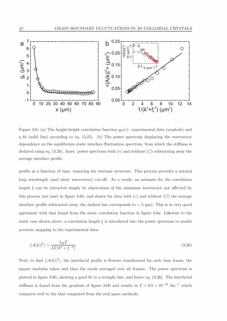
42 GRAIN BOUNDARY FLUCTUATIONS IN 2D COLLOIDAL CRYSTALS
0.1 1
0.1
1
0 2 4 6 8 10 12 140.00
0.05
0.10
0.15
0.20
0.25
0 10 20 30 40 50 60 70 80 90-1
0
1
2
3
4
5
6
7
g(
m)
hμ
2
x (μm)
a b
<|A
(k)|
> (
2μ
m)
2
1/(k + ) (2 -2
ξ μm )2
<|A
(k)|
>2
(m
)μ
2
k ( m )μ-1
Figure 3.6: (a) The height-height correlation function gh(x): experimental data (symbols) and
a fit (solid line) according to eq. (3.25). (b) The power spectrum displaying the wavevector
dependence on the equilibrium static interface fluctuation spectrum, from which the stiffness is
deduced using eq. (3.26). Inset: power spectrum with (◦) and without (�) subtracting away the
average interface profile.
profile as a function of time, removing the intrinsic structure. This process provides a natural
long wavelength (and short wavevector) cut-off. As a result, an estimate for the correlation
length ξ can be extracted simply by observation of the minimum wavevector not affected by
this process (see inset in figure 3.6b, and shown for data with (◦) and without (�) the average
interface profile subtracted away, the dashed line corresponds to ∼ 5 µm). This is in very good
agreement with that found from the static correlation function in figure 3.6a. Likewise to the
static case shown above, a correlation length ξ is introduced into the power spectrum to enable
accurate mapping to the experimental data:
〈|A(k)|2〉 =kBT
LΓ(k2 + ξ−2). (3.26)
Next, to find 〈|A(k)|2〉, the interfacial profile is Fourier transformed for each time frame, the
square modulus taken and then the result averaged over all frames. The power spectrum is
plotted in figure 3.6b, showing a good fit to a straight line, and hence eq. (3.26). The interfacial
stiffness is found from the gradient of figure 3.6b and results in Γ = 3.5× 10⁻¹⁵ Jm−1 which
compares well to the that computed from the real space methods.
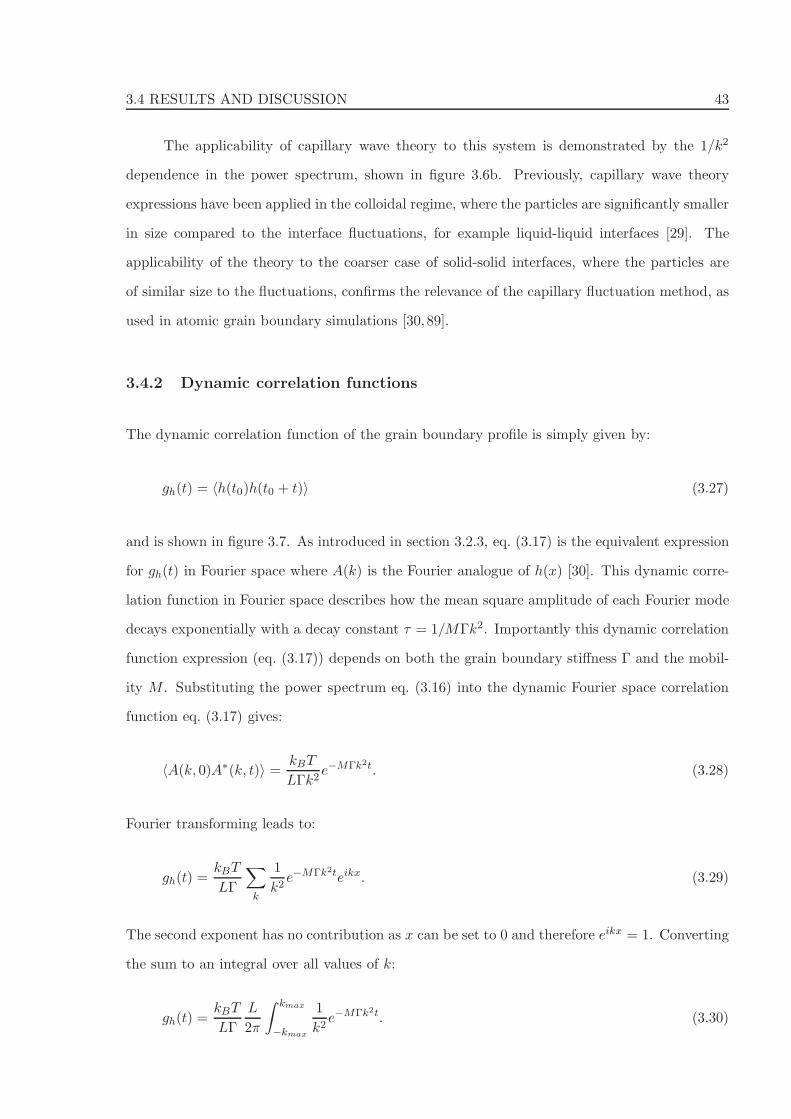
3.4 RESULTS AND DISCUSSION 43
The applicability of capillary wave theory to this system is demonstrated by the 1/k2
dependence in the power spectrum, shown in figure 3.6b. Previously, capillary wave theory
expressions have been applied in the colloidal regime, where the particles are significantly smaller
in size compared to the interface fluctuations, for example liquid-liquid interfaces [29]. The
applicability of the theory to the coarser case of solid-solid interfaces, where the particles are
of similar size to the fluctuations, confirms the relevance of the capillary fluctuation method, as
used in atomic grain boundary simulations [30,89].
3.4.2 Dynamic correlation functions
The dynamic correlation function of the grain boundary profile is simply given by:
gh(t) = 〈h(t0)h(t0 + t)〉 (3.27)
and is shown in figure 3.7. As introduced in section 3.2.3, eq. (3.17) is the equivalent expression
for gh(t) in Fourier space where A(k) is the Fourier analogue of h(x) [30]. This dynamic corre-
lation function in Fourier space describes how the mean square amplitude of each Fourier mode
decays exponentially with a decay constant τ = 1/MΓk2. Importantly this dynamic correlation
function expression (eq. (3.17)) depends on both the grain boundary stiffness Γ and the mobil-
ity M . Substituting the power spectrum eq. (3.16) into the dynamic Fourier space correlation
function eq. (3.17) gives:
〈A(k, 0)A∗(k, t)〉 =kBT
LΓk2e−MΓk2t. (3.28)
Fourier transforming leads to:
gh(t) =kBT
LΓ
∑
k
1
k2e−MΓk2teikx. (3.29)
The second exponent has no contribution as x can be set to 0 and therefore eikx = 1. Converting
the sum to an integral over all values of k:
gh(t) =kBT
LΓ
L
2π
∫ kmax
−kmax
1
k2e−MΓk2t. (3.30)
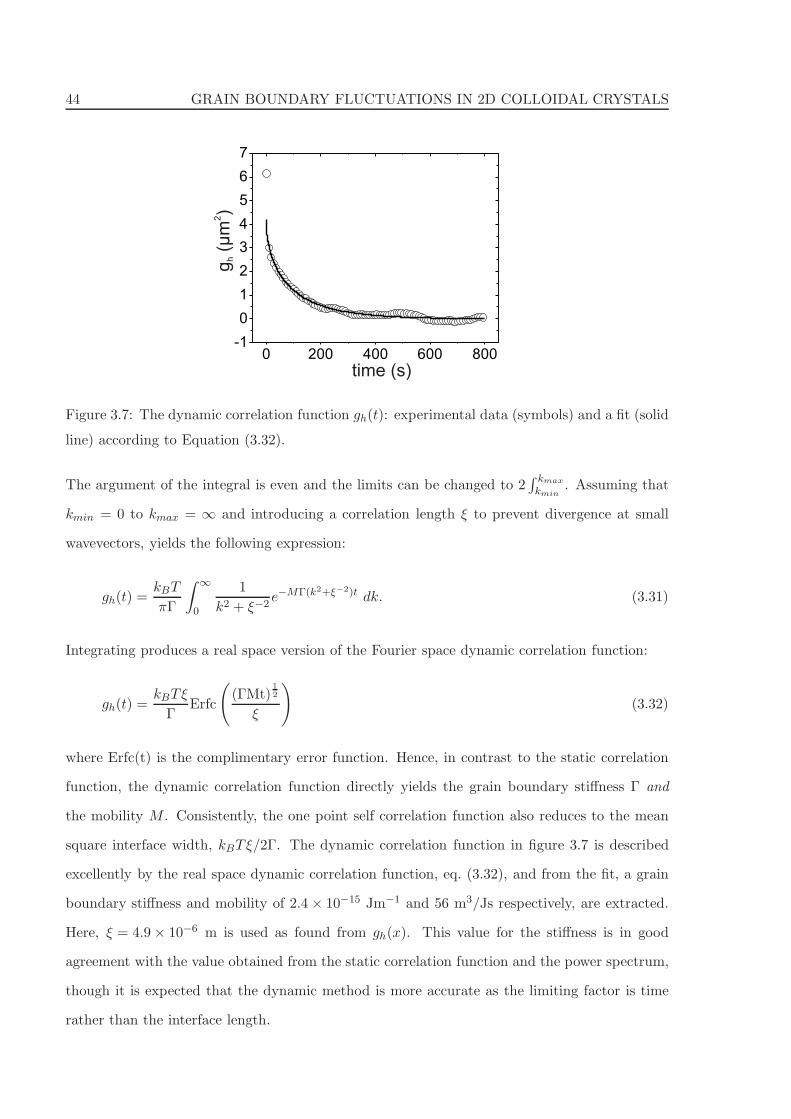
44 GRAIN BOUNDARY FLUCTUATIONS IN 2D COLLOIDAL CRYSTALS
0 200 400 600 800-1
0
1
2
3
4
5
6
7
g(
hμ
m)
2
time (s)
Figure 3.7: The dynamic correlation function gh(t): experimental data (symbols) and a fit (solid
line) according to Equation (3.32).
The argument of the integral is even and the limits can be changed to 2∫ kmax
kmin. Assuming that
kmin = 0 to kmax = ∞ and introducing a correlation length ξ to prevent divergence at small
wavevectors, yields the following expression:
gh(t) =kBT
πΓ
∫ ∞
0
1
k2 + ξ−2e−MΓ(k2+ξ−2)t dk. (3.31)
Integrating produces a real space version of the Fourier space dynamic correlation function:
gh(t) =kBTξ
ΓErfc
(
(ΓMt)1
2
ξ
)
(3.32)
where Erfc(t) is the complimentary error function. Hence, in contrast to the static correlation
function, the dynamic correlation function directly yields the grain boundary stiffness Γ and
the mobility M . Consistently, the one point self correlation function also reduces to the mean
square interface width, kBTξ/2Γ. The dynamic correlation function in figure 3.7 is described
excellently by the real space dynamic correlation function, eq. (3.32), and from the fit, a grain
boundary stiffness and mobility of 2.4 × 10⁻¹⁵ Jm−1 and 56 m3/Js respectively, are extracted.
Here, ξ = 4.9× 10⁻⁶ m is used as found from gh(x). This value for the stiffness is in good
agreement with the value obtained from the static correlation function and the power spectrum,
though it is expected that the dynamic method is more accurate as the limiting factor is time
rather than the interface length.

3.4 RESULTS AND DISCUSSION 45
L <
|A
(k)|
> (
2μ
m)
3
τ (s)
<A
(k,0
)A*
time (s)0 20 40 60 80 100 120 140
0
5
10
15
20
25
30
35
40
0 100 200 300 400 500 600
0.00
0.05
0.10
0.15
0.20
0.21
0.31
0.55
1.17
a b(k
,t)>
(m
)μ
2
k ( m )μ-1
Figure 3.8: a) Decay of the amplitudes of the Fourier modes for a selection of wavevectors
and shown with exponential fits. b) For each wavevector, L〈|A(k)|2〉 is shown versus the decay
constant found from the time decay of the amplitude of that wavevector. The line represents a
line of best fit.
Next, the interfacial properties are extracted from the dynamic correlations of the inter-
facial fluctuations, but in Fourier space. As a comparison to the real space method just shown,
the reciprocal space dynamic correlation function, eq. (3.17), as described by Hoyt et al. [30] is
directly used. A few examples of the decay of the Fourier modes, 〈A(k, 0)A∗(k, t)〉 versus time,
are given in figure 3.8a. Note that the fitting is poor at short times. It is thought this is maybe
due to the sampling rate (2Hz) being significantly faster than the Brownian time (∼ 11 s (at in-
finite dilution)) creating greater correlation at short times. The decay constant, τ , in eq. (3.17)
is given by τ = 1/MΓk2, and substituting this into eq. (3.16) gives L〈|A(k)|2〉 = kBTMτ
(eq. (3.18)). Subsequently, plotting L〈|A(k)|2〉 as a function of τ , see figure 3.8b, leads to a
mobility of M = 55 m3/Js, which compares excellently to the grain boundary mobility obtained
from the dynamic height-height correlation function.
The grain boundary properties of the interfacial stiffness and mobility have been found,
and show good agreement between the standard capillary fluctuation method and that from the
real space derivations. Next, a different real space approach as developed by Trautt et al. [100]
is tested, where the random walk performed by the average interface position is used to find the
interfacial mobility.
46 GRAIN BOUNDARY FLUCTUATIONS IN 2D COLLOIDAL CRYSTALS
3.4.3 Mobility from random walk analysis
Computer simulations by Trautt et al. [100] suggest that the grain boundary mobility can also
be extracted using a fluctuation-dissipation based theorem in the limit of zero driving force.
This approach is based on the average interface position performing a one-dimensional (1D)
random walk. This is the interface-analog of the Stokes-Einstein relation for 1D diffusion of a
Brownian particle, 〈h2〉 = 2Dt where the diffusion constant D is directly proportional to the
grain boundary mobility M . The dimensionality of their result is reduced for use with a 1D
grain boundary. The resulting expression relates the average interface height h = 1L
∫ L0 h(x, t)dx
to a random walk via:
D =MkBT
L. (3.33)
A typical trajectory of the average interface position, h, for 200 s is shown in figure 3.9a with
the corresponding probability distribution shown in figure 3.9b. The distribution displays a
clear Gaussian shape confirming that the interface performs a 1D random walk and is therefore
consistent with the method suggested in [100]. As shown in figure 3.9c, the grain boundary
mobility is subsequently extracted from the time dependence of the mean square displacement.
A grain boundary mobility of 70 m3Js−1 is found from the gradient, which is again in very good
agreement with the mobility obtained from the dynamic correlation function. Note that data
for times smaller than the Brownian time (∼ 11 s at infinite dilution) are not taken into account
as the interface has had insufficient time to sample space.
3.4.4 Scaling comparisons for stiffness and mobility
To the author’s knowledge, previous values for the grain boundary stiffness and mobility in
colloidal crystals have not been reported, therefore the results are discussed in light of computer
simulations of atomic grain boundaries in 2D and 3D crystals (i.e. quasi-1D and quasi-2D grain
boundaries respectively). Typical stiffness results reported in 2D and 3D atomic simulations
are on the order of 10−11 Jm−1 [90] and 1 Jm−2 [91] respectively. This is consistent with the
stiffness scaling as ∼ kBT/lc in 2D and ∼ kBT/l2c in 3D, where lc is the characteristic length
scale, which for atomic systems is ∼ 1 A. Applying this scaling argument to a 2D colloidal
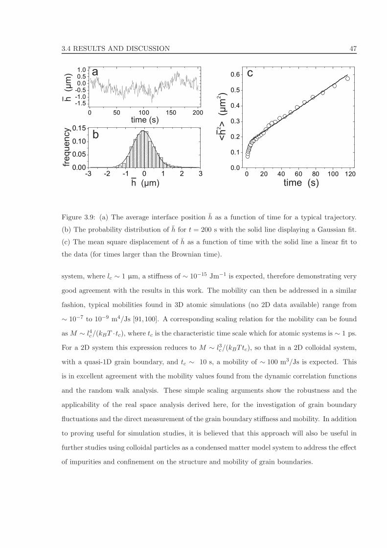
3.4 RESULTS AND DISCUSSION 47
0 50 100 150 200
-1.5-1.0-0.50.00.51.0
-3 -2 -1 0 1 2 30.00
0.05
0.10
0.15
0 20 40 60 80 100 1200.0
0.1
0.2
0.3
0.4
0.5
0.6
h μm)(
time (s)
fre
qu
en
cy
h
(m
)μ
<h
> (
m)
22
μ
a
b
time (s)
c
Figure 3.9: (a) The average interface position h as a function of time for a typical trajectory.
(b) The probability distribution of h for t = 200 s with the solid line displaying a Gaussian fit.
(c) The mean square displacement of h as a function of time with the solid line a linear fit to
the data (for times larger than the Brownian time).
system, where lc ∼ 1 µm, a stiffness of ∼ 10−15 Jm−1 is expected, therefore demonstrating very
good agreement with the results in this work. The mobility can then be addressed in a similar
fashion, typical mobilities found in 3D atomic simulations (no 2D data available) range from
∼ 10−7 to 10−9 m4/Js [91,100]. A corresponding scaling relation for the mobility can be found
as M ∼ l4c/(kBT ·tc), where tc is the characteristic time scale which for atomic systems is ∼ 1 ps.
For a 2D system this expression reduces to M ∼ l3c/(kBT tc), so that in a 2D colloidal system,
with a quasi-1D grain boundary, and tc ∼ 10 s, a mobility of ∼ 100 m3/Js is expected. This
is in excellent agreement with the mobility values found from the dynamic correlation functions
and the random walk analysis. These simple scaling arguments show the robustness and the
applicability of the real space analysis derived here, for the investigation of grain boundary
fluctuations and the direct measurement of the grain boundary stiffness and mobility. In addition
to proving useful for simulation studies, it is believed that this approach will also be useful in
further studies using colloidal particles as a condensed matter model system to address the effect
of impurities and confinement on the structure and mobility of grain boundaries.
48 GRAIN BOUNDARY FLUCTUATIONS IN 2D COLLOIDAL CRYSTALS
3.5 Conclusions
The interfacial fluctuations of a quasi-1D grain boundary have been experimentally analysed in
a 2D colloidal crystal. Expressions pertaining from capillary wave theory have been found to
be applicable to these interfaces. The interfacial parameters, the mobility and stiffness, have
been calculated from real space versions of the spatial and dynamical capillary wave theory
expressions as used in the capillary fluctuation method. Good agreement is found between the
methods derived here and from the dynamic and spatial correlation functions in Fourier space
using the standard capillary fluctuation method. The prediction from simulation, that the mean
square displacement of the average interface position can be used to find the mobility, has also
been experimentally demonstrated and shows excellent agreement with all methods. Lastly, the
grain boundary results found in these colloidal crystals display good agreement with those found
from atomic grain boundary simulations using simple scaling arguments.
Acknowledgments
This work was done in collaboration with Dirk Aarts. Gert Aarts, Anna Maciolek and Klaus
Mecke are thanked for useful discussions and Alice Thorneywork and Michael Juniper for criti-
cally reading the manuscript.
Chapter 4
Supercooled dynamics of grain
boundary particles
ABSTRACT
The dynamics of particles within a grain boundary are investigated in a two-dimensional col-
loidal crystal. The mean square displacement of the grain boundary particles displays a clear
plateau followed by an upswing indicative of cage breaking. The van Hove correlation functions
and the non-Gaussian parameter show that the grain boundary particle dynamics are highly
heterogeneous. Furthermore, clusters of cooperatively moving particles are identified and the
time-dependence of the weight-averaged mean cluster size analysed. Good correlation between
the behaviour of the mean square displacement, the time dependence of the non-Gaussian param-
eter and the cluster size, as also reported for various supercooled systems is found. These results
provide experimental support for the similarity between particle dynamics in grain boundaries
and those in supercooled liquids, as suggested by recent computer simulations.
This chapter is based on and reprinted with permission from [Thomas O. E. Skinner, Dirk G.
A. L. Aarts and Roel P. A. Dullens, (2011), Supercooled dynamics of grain-boundary particles in
colloidal crystals, J. Chem. Phys. 135, 124711]. Copyright 2011, American Institute of Physics.
49
50 SUPERCOOLED DYNAMICS OF GRAIN BOUNDARY PARTICLES
4.1 Introduction
Grain boundaries (GBs) are the interface between adjacent crystals of differing orientation.
Material microstructure is characterised by the network formed by GBs and other defects within
a material, which then determine material properties including corrosion resistance, conductivity
and strength [75, 77]. The development of most modern materials therefore requires precise
control over the microstructural evolution during manufacture. As the structure and dynamics
of GBs play an important role in microstructural development, GBs have been extensively
studied in simulations [30,90–92,94,100,126] and experiments [87,97,117,120,132–134]. Studies
of the dynamics of individual grain boundary particles however, have been mainly addressed
using simulations [32, 110]. Although the structure of grain boundaries in atomic systems has
been studied in experiment [84,86,135], the time resolution needed to follow the movements of
individual atoms is not yet attainable. The dynamics of particles at crystal boundaries is known
to be important in several areas: the onset of melting [98], in the crystallisation of hard sphere
glasses [136] and in the dynamics of dislocations [96,97].
It has been suggested many times, as early as about 1900, that grain boundaries may
have an amorphous structure [31]. Due to the confinement of the atoms between the crystals, it
was postulated that the atoms within a grain boundary may also exhibit dynamics akin to glass
forming liquids [111,137–139]. Strong support for this hypothesis was more recently provided by
molecular dynamics simulations [32,111] of high temperature grain boundaries, which indicated
that the dynamics of GB particles are heterogeneous and show cooperative motion, which is also
typically found in the particle dynamics of supercooled and glass-forming liquids [140–144]. Note
that during publication of this work [145] a related study on grain boundary particle behaviour
was published by Nagamanasa et al. [146], which came to similar conclusions.
High temperature grain boundary behaviour can have important consequences for prop-
erties relevant to materials processing, including GB strength [147] and mobility [148]. This un-
derlines the importance of the need to understand the dynamics of particles in grain boundaries
to ultimately enable greater microstructural control through grain boundary engineering [149].
Colloidal systems have proved to be very useful model systems with which to study GBs ex-
perimentally [23, 96, 98, 99, 134]. In this work, the dynamics of particles constituting GBs in
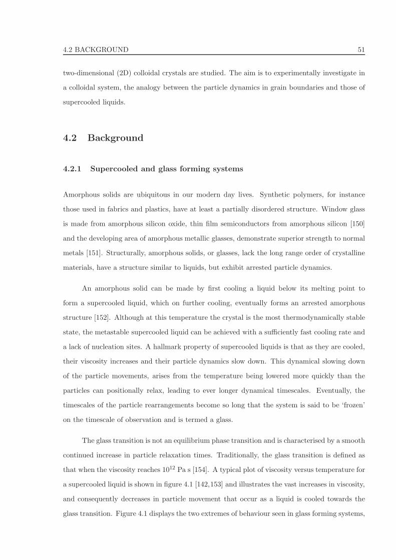
4.2 BACKGROUND 51
two-dimensional (2D) colloidal crystals are studied. The aim is to experimentally investigate in
a colloidal system, the analogy between the particle dynamics in grain boundaries and those of
supercooled liquids.
4.2 Background
4.2.1 Supercooled and glass forming systems
Amorphous solids are ubiquitous in our modern day lives. Synthetic polymers, for instance
those used in fabrics and plastics, have at least a partially disordered structure. Window glass
is made from amorphous silicon oxide, thin film semiconductors from amorphous silicon [150]
and the developing area of amorphous metallic glasses, demonstrate superior strength to normal
metals [151]. Structurally, amorphous solids, or glasses, lack the long range order of crystalline
materials, have a structure similar to liquids, but exhibit arrested particle dynamics.
An amorphous solid can be made by first cooling a liquid below its melting point to
form a supercooled liquid, which on further cooling, eventually forms an arrested amorphous
structure [152]. Although at this temperature the crystal is the most thermodynamically stable
state, the metastable supercooled liquid can be achieved with a sufficiently fast cooling rate and
a lack of nucleation sites. A hallmark property of supercooled liquids is that as they are cooled,
their viscosity increases and their particle dynamics slow down. This dynamical slowing down
of the particle movements, arises from the temperature being lowered more quickly than the
particles can positionally relax, leading to ever longer dynamical timescales. Eventually, the
timescales of the particle rearrangements become so long that the system is said to be ‘frozen’
on the timescale of observation and is termed a glass.
The glass transition is not an equilibrium phase transition and is characterised by a smooth
continued increase in particle relaxation times. Traditionally, the glass transition is defined as
that when the viscosity reaches 1012 Pa s [154]. A typical plot of viscosity versus temperature for
a supercooled liquid is shown in figure 4.1 [142,153] and illustrates the vast increases in viscosity,
and consequently decreases in particle movement that occur as a liquid is cooled towards the
glass transition. Figure 4.1 displays the two extremes of behaviour seen in glass forming systems,
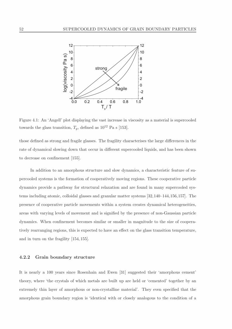
52 SUPERCOOLED DYNAMICS OF GRAIN BOUNDARY PARTICLES
T / Tg
log(v
iscosity P
a s
)strong
fragile
0.0 0.2 0.4 0.6 0.8 1.0-4
-2
0
2
4
6
8
10
12
-4
-2
0
2
4
6
8
10
12
Figure 4.1: An ‘Angell’ plot displaying the vast increase in viscosity as a material is supercooled
towards the glass transition, Tg, defined as 1012 Pa s [153].
those defined as strong and fragile glasses. The fragility characterises the large differences in the
rate of dynamical slowing down that occur in different supercooled liquids, and has been shown
to decrease on confinement [155].
In addition to an amorphous structure and slow dynamics, a characteristic feature of su-
percooled systems is the formation of cooperatively moving regions. These cooperative particle
dynamics provide a pathway for structural relaxation and are found in many supercooled sys-
tems including atomic, colloidal glasses and granular matter systems [32,140–144,156,157]. The
presence of cooperative particle movements within a system creates dynamical heterogeneities,
areas with varying levels of movement and is signified by the presence of non-Gaussian particle
dynamics. When confinement becomes similar or smaller in magnitude to the size of coopera-
tively rearranging regions, this is expected to have an effect on the glass transition temperature,
and in turn on the fragility [154,155].
4.2.2 Grain boundary structure
It is nearly a 100 years since Rosenhain and Ewen [31] suggested their ‘amorphous cement’
theory, where ‘the crystals of which metals are built up are held or ‘cemented’ together by an
extremely thin layer of amorphous or non-crystalline material’. They even specified that the
amorphous grain boundary region is ‘identical with or closely analogous to the condition of a
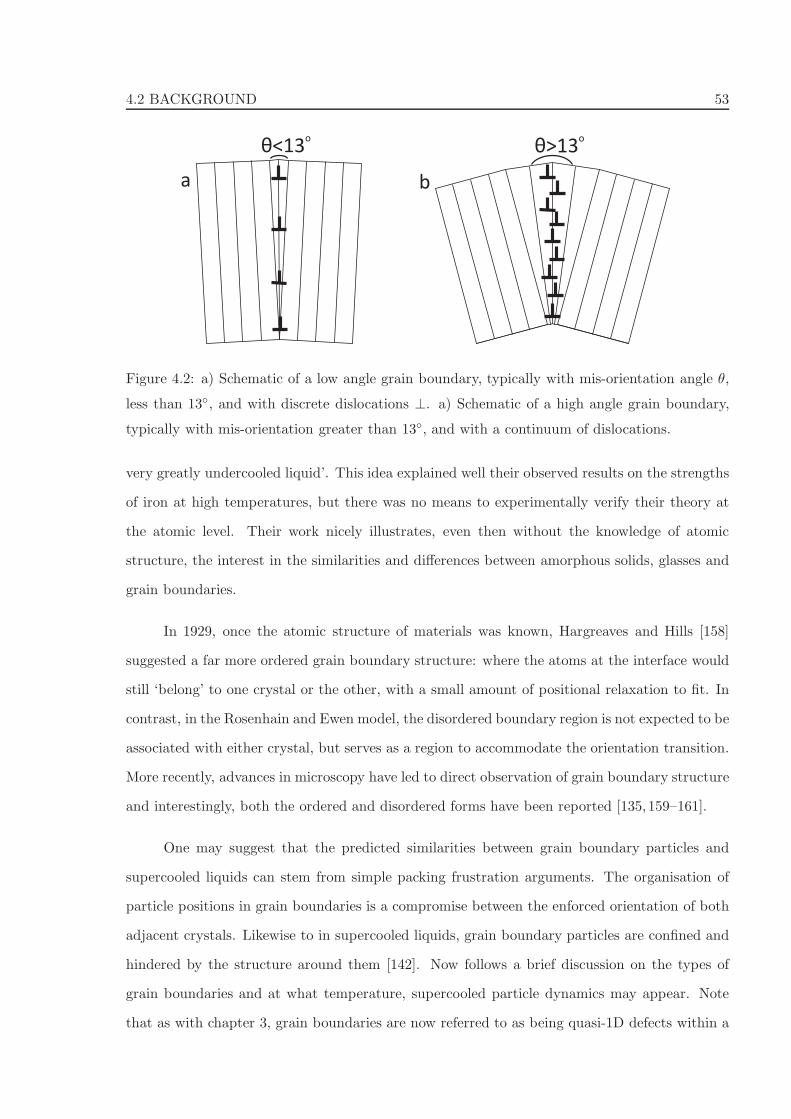
4.2 BACKGROUND 53
a b
θ>13o
θ<13o
Figure 4.2: a) Schematic of a low angle grain boundary, typically with mis-orientation angle θ,
less than 13◦, and with discrete dislocations ⊥. a) Schematic of a high angle grain boundary,
typically with mis-orientation greater than 13◦, and with a continuum of dislocations.
very greatly undercooled liquid’. This idea explained well their observed results on the strengths
of iron at high temperatures, but there was no means to experimentally verify their theory at
the atomic level. Their work nicely illustrates, even then without the knowledge of atomic
structure, the interest in the similarities and differences between amorphous solids, glasses and
grain boundaries.
In 1929, once the atomic structure of materials was known, Hargreaves and Hills [158]
suggested a far more ordered grain boundary structure: where the atoms at the interface would
still ‘belong’ to one crystal or the other, with a small amount of positional relaxation to fit. In
contrast, in the Rosenhain and Ewen model, the disordered boundary region is not expected to be
associated with either crystal, but serves as a region to accommodate the orientation transition.
More recently, advances in microscopy have led to direct observation of grain boundary structure
and interestingly, both the ordered and disordered forms have been reported [135,159–161].
One may suggest that the predicted similarities between grain boundary particles and
supercooled liquids can stem from simple packing frustration arguments. The organisation of
particle positions in grain boundaries is a compromise between the enforced orientation of both
adjacent crystals. Likewise to in supercooled liquids, grain boundary particles are confined and
hindered by the structure around them [142]. Now follows a brief discussion on the types of
grain boundaries and at what temperature, supercooled particle dynamics may appear. Note
that as with chapter 3, grain boundaries are now referred to as being quasi-1D defects within a
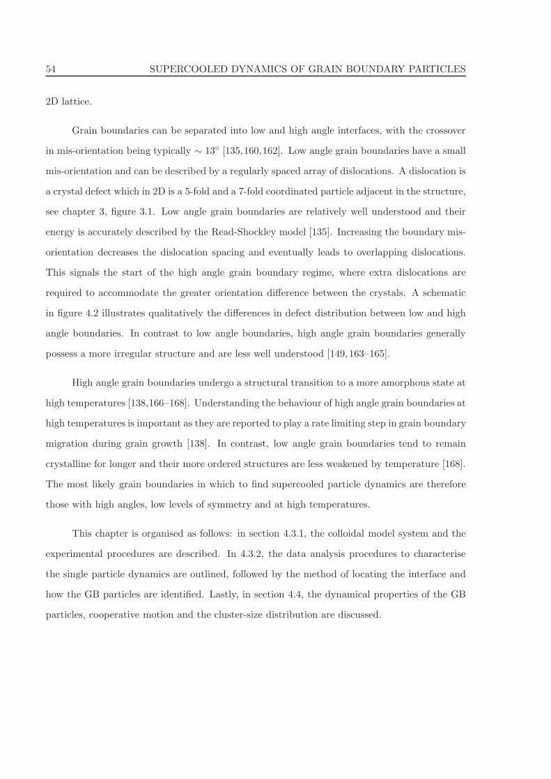
54 SUPERCOOLED DYNAMICS OF GRAIN BOUNDARY PARTICLES
2D lattice.
Grain boundaries can be separated into low and high angle interfaces, with the crossover
in mis-orientation being typically ∼ 13◦ [135,160,162]. Low angle grain boundaries have a small
mis-orientation and can be described by a regularly spaced array of dislocations. A dislocation is
a crystal defect which in 2D is a 5-fold and a 7-fold coordinated particle adjacent in the structure,
see chapter 3, figure 3.1. Low angle grain boundaries are relatively well understood and their
energy is accurately described by the Read-Shockley model [135]. Increasing the boundary mis-
orientation decreases the dislocation spacing and eventually leads to overlapping dislocations.
This signals the start of the high angle grain boundary regime, where extra dislocations are
required to accommodate the greater orientation difference between the crystals. A schematic
in figure 4.2 illustrates qualitatively the differences in defect distribution between low and high
angle boundaries. In contrast to low angle boundaries, high angle grain boundaries generally
possess a more irregular structure and are less well understood [149,163–165].
High angle grain boundaries undergo a structural transition to a more amorphous state at
high temperatures [138,166–168]. Understanding the behaviour of high angle grain boundaries at
high temperatures is important as they are reported to play a rate limiting step in grain boundary
migration during grain growth [138]. In contrast, low angle grain boundaries tend to remain
crystalline for longer and their more ordered structures are less weakened by temperature [168].
The most likely grain boundaries in which to find supercooled particle dynamics are therefore
those with high angles, low levels of symmetry and at high temperatures.
This chapter is organised as follows: in section 4.3.1, the colloidal model system and the
experimental procedures are described. In 4.3.2, the data analysis procedures to characterise
the single particle dynamics are outlined, followed by the method of locating the interface and
how the GB particles are identified. Lastly, in section 4.4, the dynamical properties of the GB
particles, cooperative motion and the cluster-size distribution are discussed.
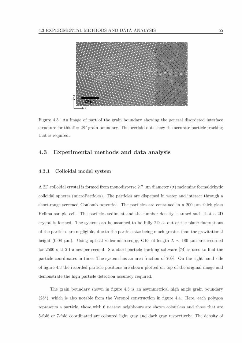
4.3 EXPERIMENTAL METHODS AND DATA ANALYSIS 55
x
y
Figure 4.3: An image of part of the grain boundary showing the general disordered interface
structure for this θ = 28◦ grain boundary. The overlaid dots show the accurate particle tracking
that is required.
4.3 Experimental methods and data analysis
4.3.1 Colloidal model system
A 2D colloidal crystal is formed from monodisperse 2.7 µm diameter (σ) melamine formaldehyde
colloidal spheres (microParticles). The particles are dispersed in water and interact through a
short-range screened Coulomb potential. The particles are contained in a 200 µm thick glass
Hellma sample cell. The particles sediment and the number density is tuned such that a 2D
crystal is formed. The system can be assumed to be fully 2D as out of the plane fluctuations
of the particles are negligible, due to the particle size being much greater than the gravitational
height (0.08 µm). Using optical video-microscopy, GBs of length L ∼ 180 µm are recorded
for 2500 s at 2 frames per second. Standard particle tracking software [74] is used to find the
particle coordinates in time. The system has an area fraction of 70%. On the right hand side
of figure 4.3 the recorded particle positions are shown plotted on top of the original image and
demonstrate the high particle detection accuracy required.
The grain boundary shown in figure 4.3 is an asymmetrical high angle grain boundary
(28◦), which is also notable from the Voronoi construction in figure 4.4. Here, each polygon
represents a particle, those with 6 nearest neighbours are shown colourless and those that are
5-fold or 7-fold coordinated are coloured light gray and dark gray respectively. The density of

56 SUPERCOOLED DYNAMICS OF GRAIN BOUNDARY PARTICLES
Figure 4.4: A Voronoi construction showing the location of the dislocations in the grain bound-
ary. Each particle is displayed as a polygon with the number of sides and shade representing
its coordination number. 6-fold particles are coloured white, and disclinations corresponding to
particles with 5 and 7 nearest neighbours are coloured light gray and dark gray respectively.
these dislocations is high and continuous, as expected for a high angle grain boundary [135]. In
a colloidal system, particle density can be interpreted as an inverse temperature scale. Hence,
to model a high temperature grain boundary the crystal number density is set, as shown, to be
sufficiently high for crystallisation, but low enough such that there is noticeable free volume in
the interface, see figure 4.3.
4.3.2 Single particle dynamics
The statistical techniques that will be applied to the coordinates of the grain boundary particles
in order to analyse their movement are introduced here. The dynamics of the single particles
are characterised by the self part of the van Hove correlation function [169], Gs(x, t), which is
the probability distribution that a particle has traveled a distance x in a time interval t:
Gs(x, t) =1
N
⟨
N∑
i=1
δ (x+ xi(0)− xi(t))
⟩
, (4.1)
where N is the number of particles. The mobility of the particles can then be measured in terms
of the mean-squared displacement,⟨
x2⟩
, defined as the second moment of Gs(x, t):
⟨
x2(t)⟩
=N∑
i=1
x2(t)Gs(x, t) =1
N
N∑
i=1
[xi(t)− xi(0)]2. (4.2)
4.3 EXPERIMENTAL METHODS AND DATA ANALYSIS 57
The non-Gaussian character of the self part of the correlation function can be quantified by the
non-Gaussian parameter, α2, defined as follows:
α2(t) =
⟨
x4(t)⟩
3 〈x2(t)〉2− 1, (4.3)
where⟨
x4⟩
is the fourth moment of Gs(x, t). The heterogeneity of the particle dynamics can
therefore be found from the time development of α2, which is zero for a Gaussian distribution,
and α2 > 0 for non-Gaussian behaviour. Together, the van Hove correlation function, the mean
square displacement and the non-Gaussian parameter form useful tools for characterising the
degree, if any, of heterogeneous particle dynamics and cage breaking as is expected in glass
forming systems.
4.3.3 Interface localisation
To identify the grain boundary particles, the coordinates of the interface must first be found using
a local orientation parameter, Φ(i), assigned to each particle, i. First, the nearest neighbour,
nc, coordinates, ~rj , of every particle are found using a Delaunay triangulation. Next, the angle
θj = tan−1[(yj − yi)/(xj − xi)], where (−π ≤ θj ≤ π), subtended from the central particle, i, to
each of its nearest neighbours, j, is obtained. The local orientation parameter, Φ(i) = 1nc
∑
j θj,
yields a measure for the orientation of the particle. It corresponds to the orientation of the
(1,1)-axis of the crystal – that the particle would be in – relative to the (horizontal) x-axis.
Each frame is subsequently split into bins of approximately the particle diameter, perpendicular
to the interface direction. The local orientation parameter is then plotted across the interface as
shown inset in figure 4.5a. A tangent-hyperbolic fit to this profile gives the interface position for
each bin. As a result, the interface height, hexp(x, t) is obtained for distance along the interface,
x, for all times, t. The resulting interface position is plotted as a white solid line in figure 4.5a.
4.3.4 Identification of grain boundary particles
The identification of the particles which constitute the grain boundary is a subtle procedure.
Grain boundaries are dynamic, with some particles frequently changing identity between crystal
and grain boundary. In addition, due to fluctuations in the local orientation, the amount of
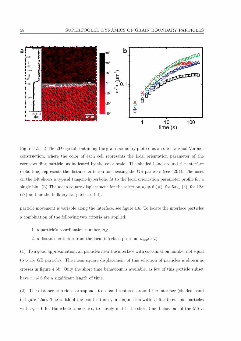
58 SUPERCOOLED DYNAMICS OF GRAIN BOUNDARY PARTICLES
1 10 100
0.1
time (s)
<r
> (
m)
22
μ
20o
10o
0o
-10o
-20o
-30o
-20 0 20
0
50
100
150
200
h(m
m)
orientation
(degrees)
30oa b
-2 0 0 20
0
50
1 00
1 50
2 00
Φ(i)
he
xp(μ
m)
Figure 4.5: a) The 2D crystal containing the grain boundary plotted as an orientational Voronoi
construction, where the color of each cell represents the local orientation parameter of the
corresponding particle, as indicated by the color scale. The shaded band around the interface
(solid line) represents the distance criterion for locating the GB particles (see 4.3.4). The inset
on the left shows a typical tangent-hyperbolic fit to the local orientation parameter profile for a
single bin. (b) The mean square displacement for the selection nc 6= 6 (×), for 5σnc (◦), for 12σ
(△) and for the bulk crystal particles (�).
particle movement is variable along the interface, see figure 4.6. To locate the interface particles
a combination of the following two criteria are applied:
1. a particle’s coordination number, nc;
2. a distance criterion from the local interface position, hexp(x, t).
(1) To a good approximation, all particles near the interface with coordination number not equal
to 6 are GB particles. The mean square displacement of this selection of particles is shown as
crosses in figure 4.5b. Only the short time behaviour is available, as few of this particle subset
have nc 6= 6 for a significant length of time.
(2) The distance criterion corresponds to a band centered around the interface (shaded band
in figure 4.5a). The width of the band is tuned, in conjunction with a filter to cut out particles
with nc = 6 for the whole time series, to closely match the short time behaviour of the MSD,
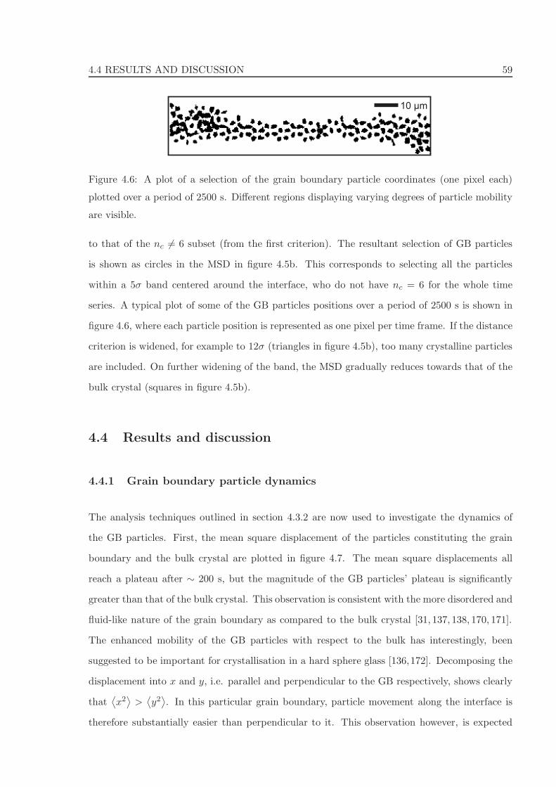
4.4 RESULTS AND DISCUSSION 59
10 mμ
Figure 4.6: A plot of a selection of the grain boundary particle coordinates (one pixel each)
plotted over a period of 2500 s. Different regions displaying varying degrees of particle mobility
are visible.
to that of the nc 6= 6 subset (from the first criterion). The resultant selection of GB particles
is shown as circles in the MSD in figure 4.5b. This corresponds to selecting all the particles
within a 5σ band centered around the interface, who do not have nc = 6 for the whole time
series. A typical plot of some of the GB particles positions over a period of 2500 s is shown in
figure 4.6, where each particle position is represented as one pixel per time frame. If the distance
criterion is widened, for example to 12σ (triangles in figure 4.5b), too many crystalline particles
are included. On further widening of the band, the MSD gradually reduces towards that of the
bulk crystal (squares in figure 4.5b).
4.4 Results and discussion
4.4.1 Grain boundary particle dynamics
The analysis techniques outlined in section 4.3.2 are now used to investigate the dynamics of
the GB particles. First, the mean square displacement of the particles constituting the grain
boundary and the bulk crystal are plotted in figure 4.7. The mean square displacements all
reach a plateau after ∼ 200 s, but the magnitude of the GB particles’ plateau is significantly
greater than that of the bulk crystal. This observation is consistent with the more disordered and
fluid-like nature of the grain boundary as compared to the bulk crystal [31, 137, 138, 170, 171].
The enhanced mobility of the GB particles with respect to the bulk has interestingly, been
suggested to be important for crystallisation in a hard sphere glass [136,172]. Decomposing the
displacement into x and y, i.e. parallel and perpendicular to the GB respectively, shows clearly
that⟨
x2⟩
>⟨
y2⟩
. In this particular grain boundary, particle movement along the interface is
therefore substantially easier than perpendicular to it. This observation however, is expected
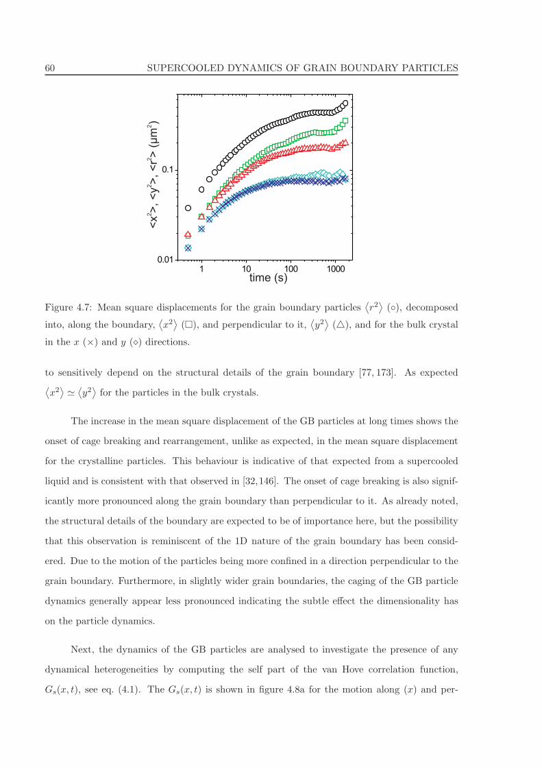
60 SUPERCOOLED DYNAMICS OF GRAIN BOUNDARY PARTICLES
1 10 100 10000.01
0.1
<x
>,
(m
)2
2μ
<y
>,
<r
>2
2
time (s)
Figure 4.7: Mean square displacements for the grain boundary particles⟨
r2⟩
(◦), decomposed
into, along the boundary,⟨
x2⟩
(�), and perpendicular to it,⟨
y2⟩
(△), and for the bulk crystal
in the x (×) and y (⋄) directions.
to sensitively depend on the structural details of the grain boundary [77, 173]. As expected⟨
x2⟩
≃⟨
y2⟩
for the particles in the bulk crystals.
The increase in the mean square displacement of the GB particles at long times shows the
onset of cage breaking and rearrangement, unlike as expected, in the mean square displacement
for the crystalline particles. This behaviour is indicative of that expected from a supercooled
liquid and is consistent with that observed in [32,146]. The onset of cage breaking is also signif-
icantly more pronounced along the grain boundary than perpendicular to it. As already noted,
the structural details of the boundary are expected to be of importance here, but the possibility
that this observation is reminiscent of the 1D nature of the grain boundary has been consid-
ered. Due to the motion of the particles being more confined in a direction perpendicular to the
grain boundary. Furthermore, in slightly wider grain boundaries, the caging of the GB particle
dynamics generally appear less pronounced indicating the subtle effect the dimensionality has
on the particle dynamics.
Next, the dynamics of the GB particles are analysed to investigate the presence of any
dynamical heterogeneities by computing the self part of the van Hove correlation function,
Gs(x, t), see eq. (4.1). The Gs(x, t) is shown in figure 4.8a for the motion along (x) and per-
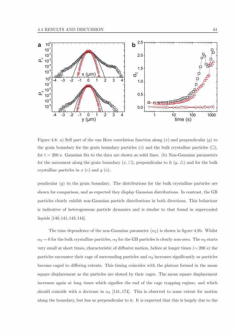
4.4 RESULTS AND DISCUSSION 61
-4 -3 -2 -1 0 1 2 3 4
10-5
10-4
10-3
10-2
10-1
100
-4 -3 -2 -1 0 1 2 3 4
10-5
10-4
10-3
10-2
10-1
100
1 10 100 1000
0.0
0.5
1.0
1.5
2.0
2.5
time (s)
α2
Px
Py
y ( m)μ
x ( m)μ
a b
Figure 4.8: a) Self part of the van Hove correlation function along (x) and perpendicular (y) to
the grain boundary for the grain boundary particles (◦) and the bulk crystalline particles (�),
for t = 200 s. Gaussian fits to the data are shown as solid lines. (b) Non-Gaussian parameters
for the movement along the grain boundary (x, �), perpendicular to it (y, △) and for the bulk
crystalline particles in x (◦) and y (⋄).
pendicular (y) to the grain boundary. The distributions for the bulk crystalline particles are
shown for comparison, and as expected they display Gaussian distributions. In contrast, the GB
particles clearly exhibit non-Gaussian particle distributions in both directions. This behaviour
is indicative of heterogeneous particle dynamics and is similar to that found in supercooled
liquids [140,141,143,144].
The time dependence of the non-Gaussian parameter (α2) is shown in figure 4.8b. Whilst
α2 ∼ 0 for the bulk crystalline particles, α2 for the GB particles is clearly non-zero. The α2 starts
very small at short times, characteristic of diffusive motion, before at longer times (∼ 200 s) the
particles encounter their cage of surrounding particles and α2 increases significantly as particles
become caged to differing extents. This timing coincides with the plateau formed in the mean
square displacement as the particles are slowed by their cages. The mean square displacement
increases again at long times which signifies the end of the cage trapping regime, and which
should coincide with a decrease in α2 [141, 174]. This is observed to some extent for motion
along the boundary, but less so perpendicular to it. It is expected that this is largely due to the
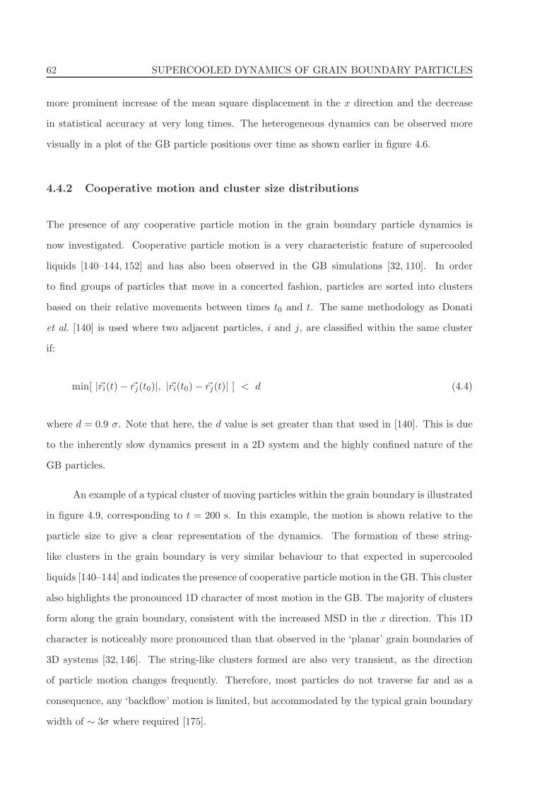
62 SUPERCOOLED DYNAMICS OF GRAIN BOUNDARY PARTICLES
more prominent increase of the mean square displacement in the x direction and the decrease
in statistical accuracy at very long times. The heterogeneous dynamics can be observed more
visually in a plot of the GB particle positions over time as shown earlier in figure 4.6.
4.4.2 Cooperative motion and cluster size distributions
The presence of any cooperative particle motion in the grain boundary particle dynamics is
now investigated. Cooperative particle motion is a very characteristic feature of supercooled
liquids [140–144, 152] and has also been observed in the GB simulations [32, 110]. In order
to find groups of particles that move in a concerted fashion, particles are sorted into clusters
based on their relative movements between times t0 and t. The same methodology as Donati
et al. [140] is used where two adjacent particles, i and j, are classified within the same cluster
if:
min[ |~ri(t)− ~rj(t0)|, |~ri(t0)− ~rj(t)| ] < d (4.4)
where d = 0.9 σ. Note that here, the d value is set greater than that used in [140]. This is due
to the inherently slow dynamics present in a 2D system and the highly confined nature of the
GB particles.
An example of a typical cluster of moving particles within the grain boundary is illustrated
in figure 4.9, corresponding to t = 200 s. In this example, the motion is shown relative to the
particle size to give a clear representation of the dynamics. The formation of these string-
like clusters in the grain boundary is very similar behaviour to that expected in supercooled
liquids [140–144] and indicates the presence of cooperative particle motion in the GB. This cluster
also highlights the pronounced 1D character of most motion in the GB. The majority of clusters
form along the grain boundary, consistent with the increased MSD in the x direction. This 1D
character is noticeably more pronounced than that observed in the ‘planar’ grain boundaries of
3D systems [32, 146]. The string-like clusters formed are also very transient, as the direction
of particle motion changes frequently. Therefore, most particles do not traverse far and as a
consequence, any ‘backflow’ motion is limited, but accommodated by the typical grain boundary
width of ∼ 3σ where required [175].
4.4 RESULTS AND DISCUSSION 63
x
y
Figure 4.9: A schematic of a typical cluster of moving particles in the grain boundary and
illustrating the cooperative nature of the particle motion. The light spheres are the particle
positions at t0 = 0 s and the dark spheres are the positions at t = 200 s. The movement is
shown relative to the particle size.
To further analyse the particle clusters formed and any cooperative motion, the distri-
bution of cluster sizes is determined. The cluster size distribution is shown in the log-lin plot
in figure 4.10a where P (n) is the probability of finding a cluster containing n grain boundary
particles. The nearly straight line distributions in figure 4.10a indicate that the cluster size dis-
tributions are approximately exponential, as is also observed in supercooled and glass-forming
systems [32,174,176]. The cluster size distributions are also highly dependent on the observation
time window, t. To quantify this time dependence, the weight-averaged mean cluster size, Sw,
is calculated as a function of t [174,176]:
Sw(t) =
⟨
n2(t)⟩
〈n(t)〉=
∑
n2(t)P (n(t))∑
n(t)P (n(t)). (4.5)
Any clusters formed at short times are random due to the particle motion still being uncorrelated.
Therefore the contribution from random clusters is taken out by normalizing Sw with respect
to the average cluster size at the shortest time S0: S ≡ Sw/S0 [174,176]. The resulting average
cluster size, S, is shown as a function of time in figure 4.10b. A rapid increase is observed as the
the time window increases, reaching a maximum at ∼ 200 s, before slowly the average cluster
size decreases again at long times.
The time development of the increase in the average cluster size coincides with the forma-
tion of the plateau in the mean square displacement, see figure 4.7. At these times the particles
are encountering the cages formed by their nearest neighbours. This causes the particle mo-
tion to start to become more non-Gaussian and cooperative motion to become apparent. The
maximum average cluster size is roughly observed when the mean square displacement has fully
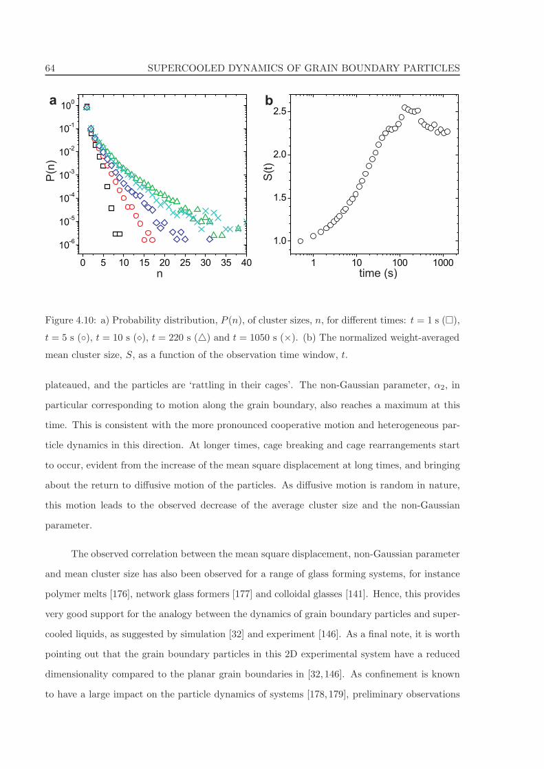
64 SUPERCOOLED DYNAMICS OF GRAIN BOUNDARY PARTICLES
0 5 10 15 20 25 30 35 40
10-6
10-5
10-4
10-3
10-2
10-1
100
1 10 100 1000
1.0
1.5
2.0
2.5
S(t
)time (s)n
P(n
)
a b
Figure 4.10: a) Probability distribution, P (n), of cluster sizes, n, for different times: t = 1 s (�),
t = 5 s (◦), t = 10 s (⋄), t = 220 s (△) and t = 1050 s (×). (b) The normalized weight-averaged
mean cluster size, S, as a function of the observation time window, t.
plateaued, and the particles are ‘rattling in their cages’. The non-Gaussian parameter, α2, in
particular corresponding to motion along the grain boundary, also reaches a maximum at this
time. This is consistent with the more pronounced cooperative motion and heterogeneous par-
ticle dynamics in this direction. At longer times, cage breaking and cage rearrangements start
to occur, evident from the increase of the mean square displacement at long times, and bringing
about the return to diffusive motion of the particles. As diffusive motion is random in nature,
this motion leads to the observed decrease of the average cluster size and the non-Gaussian
parameter.
The observed correlation between the mean square displacement, non-Gaussian parameter
and mean cluster size has also been observed for a range of glass forming systems, for instance
polymer melts [176], network glass formers [177] and colloidal glasses [141]. Hence, this provides
very good support for the analogy between the dynamics of grain boundary particles and super-
cooled liquids, as suggested by simulation [32] and experiment [146]. As a final note, it is worth
pointing out that the grain boundary particles in this 2D experimental system have a reduced
dimensionality compared to the planar grain boundaries in [32, 146]. As confinement is known
to have a large impact on the particle dynamics of systems [178,179], preliminary observations

4.5 CONCLUSION 65
suggest that the cluster sizes decrease for GBs of smaller width. These experimental results
may also be relevant for supercooled systems in other highly confining structures such as porous
media [34].
4.5 Conclusion
The dynamics of particles constituting grain boundaries in a 2D colloidal crystal has been
quantitatively analysed in real space and time using optical video-microscopy. The mean square
displacement of the grain boundary particles shows a pronounced plateau at intermediate times
followed by a subsequent increase at longer times. This is indicative of the supercooled nature
of the grain boundary particle dynamics. The mobility is found to be higher along the boundary
than perpendicular to it, although this is expected to be sensitive to the microscopic details of
the grain boundary structure, it is consistent with the highly confined 1D nature of the grain
boundary. The grain boundary particle dynamics are highly heterogeneous, as is evident from
the non-Gaussian shape of the self part of the van Hove correlation function, and from the time
dependence of the non-Gaussian parameter. Furthermore, cooperative motion has been observed
and analysed in terms of the time dependence of the weight averaged mean cluster size. The
observed correlation between the mean square displacement, the non-Gaussian parameter and
the mean cluster size is very similar to that found in supercooled systems [140–144,174,176,177].
This study therefore provides direct experimental evidence for the similarity between the nature
of the particle dynamics in grain boundaries and supercooled liquids as suggested by computer
simulations [32,110].
Acknowledgments
This work was done in collaboration with Dirk Aarts. Paddy Royall is thanked for useful
discussions. Alice Thorneywork and Michael Juniper are thanked for critically reading the
manuscript.

66 SUPERCOOLED DYNAMICS OF GRAIN BOUNDARY PARTICLES
Chapter 5
Structure and dynamics
in pentagonal confinement
ABSTRACT
The structural and dynamical behaviour of colloidal particles confined within a two-dimensional
(2D) pentagonal environment is studied. The confinement is created using an optical tweezer
to fix the positions of a pentagonal array of colloidal particles. Particles within the pentagonal
area are free to move. All the particles are super-paramagnetic and their interaction potential
is controlled by an external magnetic field. The behaviour of the confined particles and the
packing frustration created is studied via two contrasting pathways. In the first section, a
system consisting of 16 confined particles is melted from a crystalline to a confined liquid-like
state as the external magnetic field is reduced. In the second section, the magnetic field is
kept constant and the number of confined particles sequentially increased from 10 to 21. Re-
entrant orientational ordering and dynamically frustrated states occur as the number of confined
particles is increased.
67
68 STRUCTURE AND DYNAMICS IN PENTAGONAL CONFINEMENT
5.1 Introduction
Crystallisation in confinement is a widespread phenomenon, occurring in the natural processes
of biomineralisation [180] and freeze-thaw weathering [181], and in technological applications
including the fabrication of nanoparticles [182] and drug delivery [183]. The development and
control of these processes is dependent on understanding melting and crystallisation in these
confined volumes. Under extreme confinement, liquids can also appear to form rigid glass-like
structures above their melting temperatures, as such, this has far reaching consequences for
lubrication [184–186], hydrodynamics near walls [12] and lab-on-a-chip applications [187].
The effect of confinement on phase behaviour has been widely studied in small pores
[188–190] and in planar confinement [191]. Crystallisation is well known to differ from the bulk,
especially when the confinement is of comparable size to the particles, when excluded volume
effects become important [192–194]. The glass transition temperature has been seen to both
increase and decrease in confinement [195, 196], with the increases in viscosity and decreases
in particle motion occurring when boundary layering effects become important, the particle
movement restricted and the packing frustrated. In particular, crystallisation has been shown
to be very different in 2D systems, including in shaped confinement [197].
Colloidal systems are often used as model systems to investigate phase transitions [98,99,
198,199]. The control imparted from manipulation of their chemical and physical characteristics
allows the inter-particle potential to vary from hard sphere-like [16] through to a long range
repulsion [199]. Crystallisation and melting has been widely studied in colloidal systems, both
in 3D [98] and 2D [200–202]. Also, the effect of circular confinement on crystallisation has been
studied [197], which showed that shell rotations can cause re-entrant freezing behaviour. In this
chapter, the structure and dynamics of particles confined within a pentagonal environment is
studied. The incommensurate symmetry and high level of confinement makes this system truly
frustrated. The packing of pentagons in a circle has been analysed due to the similarities with
granular systems [203], but to the author’s knowledge there has been no study on the packing
and dynamics of circular particles confined in a pentagon.
5.2 BACKGROUND 69
5.2 Background
5.2.1 Colloidal systems in 2D confinement
Melting in two dimensional (2D) systems occurs via a dramatically different pathway to that
of the bulk [204] and occurs via a two-step process described by KTHNY theory [101–103].
This is a defect mediated two-step melting transition comprising of dislocation and disclination
pair unbinding processes. In 2D systems, a dislocation consists of two disclinations, one a
5-fold and one a 7-fold coordinated particle adjacent to each other in a crystal lattice, see
figure 3.1 in chapter 3. Melting in a 2D crystal starts with the unbinding of dislocation pairs,
disrupting the crystalline translational order. This forms an intermediate phase termed the
hexatic, characterised by short range translational and quasi-long range orientational order. A
further decrease in temperature results in a total loss of long range translational and orientational
order via dislocations unbinding into their constituent disclinations.
Another factor that can effect phase transitions under confinement is symmetry. Particles
contained within 2D circular and square confinements have shown that particle mobility and
packing arrangements are heavily affected by the imposed symmetry [197,205,206]. In circular
confinement, a greater amount of angular with respect to radial mobility is observed, resulting
in shell rotation [197, 207]. In contrast, in square confinement, the large difference to the pre-
ferred hexagonal symmetry induces packing frustration, small particle mobilities and leads to
degenerate structures forming [205].
Interestingly, colloidal particles confined in 2D circular environment have been shown
to exhibit a re-entrant ordering process during melting [197]. The system consists of super-
paramagnetic colloidal particles in a 2D plane inside a circular non-magnetic cavity. An external
magnetic field controls the inter-particle repulsion and the particles subsequently arrange in a
shell-like structure in the cavity. Upon decreasing the field, the system initially starts the
melting process via a loss of angular order between the shells. Further reduction of the magnetic
field however, sees the angular order restored, before finally the whole system melts. The
intermediate inter-shell rotation phase is mediated by the confinement creating a lower energy
barrier to rotation as compared to radial deviations.

70 STRUCTURE AND DYNAMICS IN PENTAGONAL CONFINEMENT
When the symmetry of the confinement is incommensurate to the preferred hexagonal
ordering of the particles, interesting packing frustration results. The phenomena of pentagonal
symmetry has long intrigued people due to its incompatibility with long range order and space
filling [208]. One method to induce large packing frustration, is to study how phase behaviour
is affected by pentagonal confinement.
5.2.2 Why study 5-fold symmetric structures?
In nature, 5-fold symmetry is seen as unremarkable and fairly common, examples include starfish,
molecules, fruits and many flowers [208, 209]. In contrast, in the areas of mathematics and
physics, it is seen as mysterious and troublesome; the symmetry is regarded as forbidden as 5-fold
structures cannot tile the plane. Kepler, Durer and Penrose each found solutions to this problem
by tessellating pairs of shapes to make aperiodic patterns; these contained 5-fold symmetry and
were able to fill 2D space [210, 211]. Pre the early 1980s, it was believed that ordered crystals
were always periodic and that orientational order was limited to 2,3,4 and 6 fold rotational
symmetries. However, in 1982 Shechtman discovered a 5-fold symmetric aperiodic structure in a
manganese and aluminium alloy [212]. Shortly afterwards Levine and Steinhardt [213] realised
that ‘Penrose tiling’ could be used to explain these ‘impossible crystals’, which lack translational
symmetry, and thus coined the term ‘quasicrystal’. The realisation of the existence of aperiodic
crystal structures earned Shechtman the 2011 Nobel prize for Chemistry [214].
Besides quasicrystals [209, 215], the younger field of nano-technology has also reported a
relative abundance of 5-fold symmetric structures [216,217]. Many nanoparticles and nanorods
that have been synthesised with pentagonal cross-section [216]. Here, the presence of the pen-
tagonal symmetry is often integral to the structure, for instance in creating anisotropic growth
for nano-wires [218–220]. An illustration of a nanorod with pentagonal cross section is shown
in figure 5.1. Notice the five symmetric grain boundaries and the central 5-fold disclination
at the centre. Many unrelated systems have observed the presence of 5-fold symmetric struc-
tures, but due to the unfamiliarity, the mere observation of pentagonal structures still provokes
intrigue [221–224].
This chapter is organised as follows. Firstly, the colloidal model system and the exper-
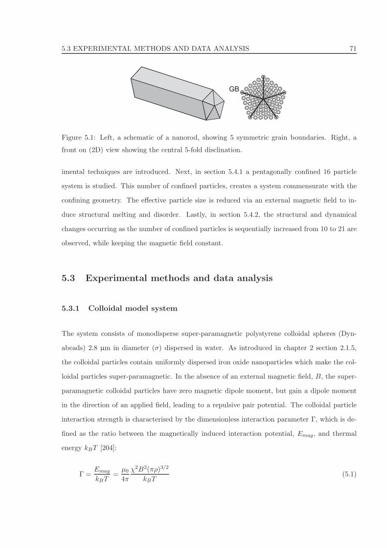
5.3 EXPERIMENTAL METHODS AND DATA ANALYSIS 71
GB
Figure 5.1: Left, a schematic of a nanorod, showing 5 symmetric grain boundaries. Right, a
front on (2D) view showing the central 5-fold disclination.
imental techniques are introduced. Next, in section 5.4.1 a pentagonally confined 16 particle
system is studied. This number of confined particles, creates a system commensurate with the
confining geometry. The effective particle size is reduced via an external magnetic field to in-
duce structural melting and disorder. Lastly, in section 5.4.2, the structural and dynamical
changes occurring as the number of confined particles is sequentially increased from 10 to 21 are
observed, while keeping the magnetic field constant.
5.3 Experimental methods and data analysis
5.3.1 Colloidal model system
The system consists of monodisperse super-paramagnetic polystyrene colloidal spheres (Dyn-
abeads) 2.8 µm in diameter (σ) dispersed in water. As introduced in chapter 2 section 2.1.5,
the colloidal particles contain uniformly dispersed iron oxide nanoparticles which make the col-
loidal particles super-paramagnetic. In the absence of an external magnetic field, B, the super-
paramagnetic colloidal particles have zero magnetic dipole moment, but gain a dipole moment
in the direction of an applied field, leading to a repulsive pair potential. The colloidal particle
interaction strength is characterised by the dimensionless interaction parameter Γ, which is de-
fined as the ratio between the magnetically induced interaction potential, Emag, and thermal
energy kBT [204]:
Γ =Emag
kBT=
µ0
4π
χ2B2(πρ)3/2
kBT(5.1)
72 STRUCTURE AND DYNAMICS IN PENTAGONAL CONFINEMENT
where ρ is the particle number density, χ the particle magnetic susceptibility and µ0 the perme-
ability of free space. This magnetic field induced control over the particle interaction potential
and state of the system acts as a from of temperature gauge, equivalent to 1/Γ.
The colloidal particle system is contained within a 200 µm thick, glass Hellma sample cell.
The particles sediment and as the particle size is much greater than the gravitational height, the
out-of-plane fluctuations of the particles are negligible. A very dilute sample is created where
there are typically 5 particles per 100 µm2 of sample cell.
5.3.2 Optical tweezing, magnetic fields and video microscopy
The sample is placed in the optical tweezer and microscopy set-up, which is described in chapter
2, section 2.2.5. As a brief recap, an optical tweezer is a highly focused laser beam that can trap
particles and move them. One laser beam is time-shared between many points to create many
‘individual’ traps using an acousto-optic deflector. The laser beam can move between these
points sufficiently quickly that, on the time-scale of the Brownian movements of the colloidal
particles, each optical trap is seen as discrete.
Within the sample cell the required number of colloidal particles, typically 31, are isolated
using the optical tweezer to a selected area of the cell, leaving a region, ∼ 100 µm in all directions
free from particles. The pentagonal confinement is created by tweezing an array of particles to
produce a pentagon shape as shown in figure 5.2a. These traps then remain on for the entirety
of the experiment to retain the pentagonal environment. An additional trap is used to add the
remaining required number of particles into the confined zone, before being switched off.
The particle spacing of the pentagonally shaped confinement is set to 10 µm. This enforced
gap leads to a lower bound on the magnetic field used of 1 mT before particles escape. To reduce
the effect of the optical tweezer on the free particles inside the pentagon, the optical tweezer trap
strength is set to the minimum value that can sustain the pentagonal environment (time-shared
20 mW). The magnetic field is increased to the required value at a rate of 0.001 mTs−1 to allow
the system to equilibrate. Using optical video-microscopy (PixeLINK CMOS camera) image
stacks are recorded at 1 Hz for 4000 s. Standard particle tracking software [74] is used to find
the colloidal particle coordinates in time, as is described in chapter 2, section 2.12.

5.3 EXPERIMENTAL METHODS AND DATA ANALYSIS 73
0 2 4 6 8 10 12 14 16 18 20
0.00
0.01
0.02
0.03
0.04
0.05
0.06
0.07
01
2
3
Distance from centre ( m)μ
Fre
quency d
ensity
a b
0 1 2 3Shell
Figure 5.2: a) 31 colloidal particles of which 16 are confined within a pentagon created by the
other 15, fixed into position (black dots overlaid) using an optical tweezer. The shells are denoted
3, 2, 1 and 0, where 0 is the central particle. Gravity and magnetic field are perpendicular to
the plane. b) Radially averaged histogram of the particle positions measured from the pentagon
centre over a period of an hour for the system to the left. The shell structure contains a central
particle and 5 particles in each of the shells 1, 2 and 3.
5.3.3 Characterising the particle environments
A shell based terminology is introduced to characterise the particle positions. The positions
of 16 confined colloidal particles in the pentagonal environment are shown in figure 5.2a, with
the radial density distributions of the same system averaged over the course of an hour shown
in figure 5.2b. The particles in figure 5.2a which are optically tweezed to create the pentagon,
are shown with dots overlaid. The positions highlighted in figure 5.2a, and the corresponding
pentagons they encompass, displays the four distinct shells within the pentagon as is evident
from the peaks in the radial histogram in figure 5.2b. Hence, a central particle and three
surrounding pentagons, denoted shells 0, 1, 2 and 3 are identified. This packing configuration is
schematically denoted as a 5,5,5,1 shell structure, i.e. three shells of 5 particles with 1 particle
at the centre. This is referred to as an ‘ideal’ configuration with a commensurate number of
particles. If particles move shells then their average radial position is used as a guide. This
terminology is used to describe the observed structures: for example 5,5,5,4 corresponds to
three shells of 5 particles with 4 particles occupying the the innermost area.
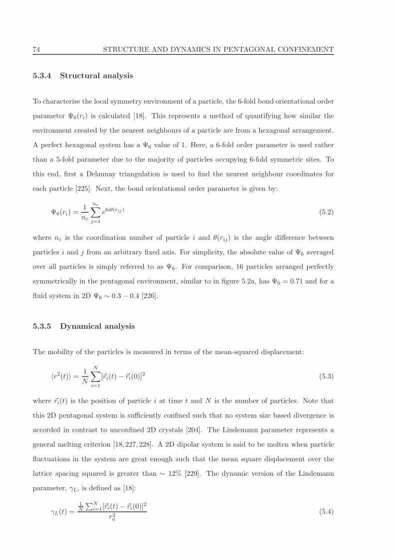
74 STRUCTURE AND DYNAMICS IN PENTAGONAL CONFINEMENT
5.3.4 Structural analysis
To characterise the local symmetry environment of a particle, the 6-fold bond orientational order
parameter Ψ6(ri) is calculated [18]. This represents a method of quantifying how similar the
environment created by the nearest neighbours of a particle are from a hexagonal arrangement.
A perfect hexagonal system has a Ψ6 value of 1. Here, a 6-fold order parameter is used rather
than a 5-fold parameter due to the majority of particles occupying 6-fold symmetric sites. To
this end, first a Delaunay triangulation is used to find the nearest neighbour coordinates for
each particle [225]. Next, the bond orientational order parameter is given by:
Ψ6(ri) =1
nc
nc∑
j=1
e6iθ(rij ) (5.2)
where nc is the coordination number of particle i and θ(rij) is the angle difference between
particles i and j from an arbitrary fixed axis. For simplicity, the absolute value of Ψ6 averaged
over all particles is simply referred to as Ψ6. For comparison, 16 particles arranged perfectly
symmetrically in the pentagonal environment, similar to in figure 5.2a, has Ψ6 = 0.71 and for a
fluid system in 2D Ψ6 ∼ 0.3 − 0.4 [226].
5.3.5 Dynamical analysis
The mobility of the particles is measured in terms of the mean-squared displacement:
〈r2(t)〉 =1
N
N∑
i=1
[~ri(t)− ~ri(0)]2 (5.3)
where ~ri(t) is the position of particle i at time t and N is the number of particles. Note that
this 2D pentagonal system is sufficiently confined such that no system size based divergence is
accorded in contrast to unconfined 2D crystals [204]. The Lindemann parameter represents a
general melting criterion [18,227,228]. A 2D dipolar system is said to be molten when particle
fluctuations in the system are great enough such that the mean square displacement over the
lattice spacing squared is greater than ∼ 12% [229]. The dynamic version of the Lindemann
parameter, γL, is defined as [18]:
γL(t) =1N
∑Ni=1[~ri(t)− ~ri(0)]
2
r2a(5.4)
5.3 EXPERIMENTAL METHODS AND DATA ANALYSIS 75
Figure 5.3: Snapshot of a Monte Carlo run for 16 confined particles. The fixed particles (black)
and the mobile particles (gray) interact via a 1/r3 potential with a hard core diameter of 1.
where ra is the mean lattice spacing.
Finally, the bond-order correlation function in time, g6(t), is calculated which describes
the decay rate of orientational correlations and is found from a dynamic correlation function of
the local bond order parameter Ψ6 [18, 204]:
g6(t) = 〈ei6[θ(t)−θ(0)]〉 (5.5)
where θ(t) is the angle of the bond between two particles and 〈〉 represents an average over all
bonds. The g6(t) can act as a melting criterion with a order-disorder transition expected from
a crystalline or hexatic phase through to a fluid in bulk 2D systems, when the long time decay
scales as g6(t) ∼ t−1/8 [230].
5.3.6 Monte Carlo Simulations
Standard Monte Carlo simulations are performed in the canonical ensemble [231] to qualitatively
mimic the experimental set-up of particles confined in a pentagonal environment. A snapshot of
a Monte Carlo system is given in figure 5.3 showing the fixed (black) and confined, but mobile
(gray) particles. Likewise to the experiment, the particles act as point dipoles with a repulsive
1/r3 interaction potential. The particles have a non-overlapping diameter of 1 and the outer
particles are fixed with a separation of 3 diameters which is comparable to the experiment. The
simulation cycles are started by equilibrating the confined particles with 103 steps per particle.
The step size is adjusted during equilibration so that the acceptance rate of the Monte Carlo
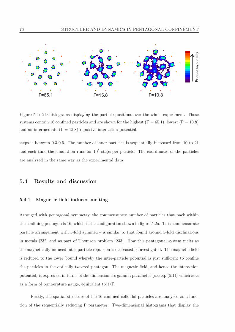
76 STRUCTURE AND DYNAMICS IN PENTAGONAL CONFINEMENT
Fre
quency d
ensity
Γ=65.1 Γ=15.8 Γ=10.8
Figure 5.4: 2D histograms displaying the particle positions over the whole experiment. These
systems contain 16 confined particles and are shown for the highest (Γ = 65.1), lowest (Γ = 10.8)
and an intermediate (Γ = 15.8) repulsive interaction potential.
steps is between 0.3-0.5. The number of inner particles is sequentially increased from 10 to 21
and each time the simulation runs for 105 steps per particle. The coordinates of the particles
are analysed in the same way as the experimental data.
5.4 Results and discussion
5.4.1 Magnetic field induced melting
Arranged with pentagonal symmetry, the commensurate number of particles that pack within
the confining pentagon is 16, which is the configuration shown in figure 5.2a. This commensurate
particle arrangement with 5-fold symmetry is similar to that found around 5-fold disclinations
in metals [232] and as part of Thomson problem [233]. How this pentagonal system melts as
the magnetically induced inter-particle repulsion is decreased is investigated. The magnetic field
is reduced to the lower bound whereby the inter-particle potential is just sufficient to confine
the particles in the optically tweezed pentagon. The magnetic field, and hence the interaction
potential, is expressed in terms of the dimensionless gamma parameter (see eq. (5.1)) which acts
as a form of temperature gauge, equivalent to 1/Γ.
Firstly, the spatial structure of the 16 confined colloidal particles are analysed as a func-
tion of the sequentially reducing Γ parameter. Two-dimensional histograms that display the
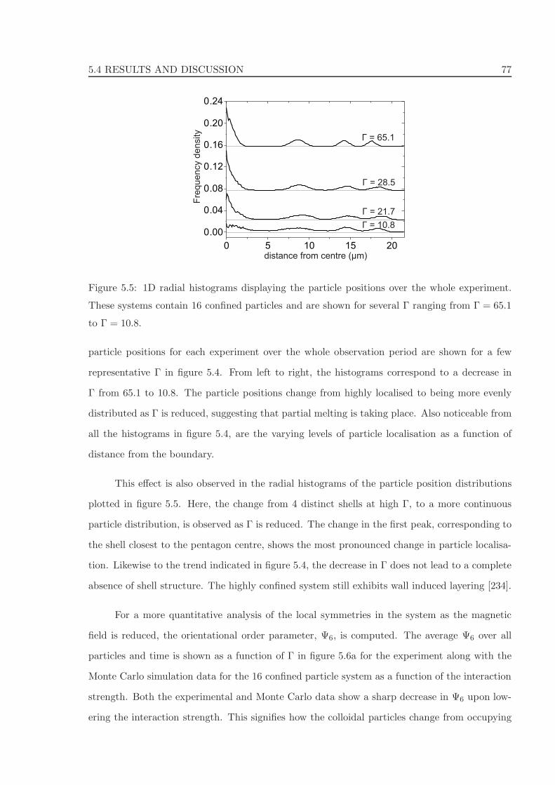
5.4 RESULTS AND DISCUSSION 77
0 5 10 15 20
0.00
0.04
0.08
0.12
0.16
0.20
0.24
distance from centre ( m)μ
Fre
quency d
ensity
Γ = 10.8
Γ = 21.7
Γ = 28.5
Γ = 65.1
Figure 5.5: 1D radial histograms displaying the particle positions over the whole experiment.
These systems contain 16 confined particles and are shown for several Γ ranging from Γ = 65.1
to Γ = 10.8.
particle positions for each experiment over the whole observation period are shown for a few
representative Γ in figure 5.4. From left to right, the histograms correspond to a decrease in
Γ from 65.1 to 10.8. The particle positions change from highly localised to being more evenly
distributed as Γ is reduced, suggesting that partial melting is taking place. Also noticeable from
all the histograms in figure 5.4, are the varying levels of particle localisation as a function of
distance from the boundary.
This effect is also observed in the radial histograms of the particle position distributions
plotted in figure 5.5. Here, the change from 4 distinct shells at high Γ, to a more continuous
particle distribution, is observed as Γ is reduced. The change in the first peak, corresponding to
the shell closest to the pentagon centre, shows the most pronounced change in particle localisa-
tion. Likewise to the trend indicated in figure 5.4, the decrease in Γ does not lead to a complete
absence of shell structure. The highly confined system still exhibits wall induced layering [234].
For a more quantitative analysis of the local symmetries in the system as the magnetic
field is reduced, the orientational order parameter, Ψ6, is computed. The average Ψ6 over all
particles and time is shown as a function of Γ in figure 5.6a for the experiment along with the
Monte Carlo simulation data for the 16 confined particle system as a function of the interaction
strength. Both the experimental and Monte Carlo data show a sharp decrease in Ψ6 upon low-
ering the interaction strength. This signifies how the colloidal particles change from occupying
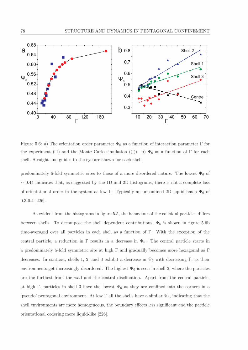
78 STRUCTURE AND DYNAMICS IN PENTAGONAL CONFINEMENT
0 40 80 120 1600.40
0.44
0.48
0.52
0.56
0.60
0.64
0.68
10 20 30 40 50 60 70
0.3
0.4
0.5
0.6
0.7
0.8 Shell 2
Shell 3
Shell 1
Centre
Γ
Ψ6
Γ
Ψ6
a b
Figure 5.6: a) The orientation order parameter Ψ6 as a function of interaction parameter Γ for
the experiment (�) and the Monte Carlo simulation (©). b) Ψ6 as a function of Γ for each
shell. Straight line guides to the eye are shown for each shell.
predominately 6-fold symmetric sites to those of a more disordered nature. The lowest Ψ6 of
∼ 0.44 indicates that, as suggested by the 1D and 2D histograms, there is not a complete loss
of orientational order in the system at low Γ. Typically an unconfined 2D liquid has a Ψ6 of
0.3-0.4 [226].
As evident from the histograms in figure 5.5, the behaviour of the colloidal particles differs
between shells. To decompose the shell dependent contributions, Ψ6 is shown in figure 5.6b
time-averaged over all particles in each shell as a function of Γ. With the exception of the
central particle, a reduction in Γ results in a decrease in Ψ6. The central particle starts in
a predominately 5-fold symmetric site at high Γ and gradually becomes more hexagonal as Γ
decreases. In contrast, shells 1, 2, and 3 exhibit a decrease in Ψ6 with decreasing Γ, as their
environments get increasingly disordered. The highest Ψ6 is seen in shell 2, where the particles
are the furthest from the wall and the central disclination. Apart from the central particle,
at high Γ, particles in shell 3 have the lowest Ψ6 as they are confined into the corners in a
‘pseudo’ pentagonal environment. At low Γ all the shells have a similar Ψ6, indicating that the
shell environments are more homogeneous, the boundary effects less significant and the particle
orientational ordering more liquid-like [226].
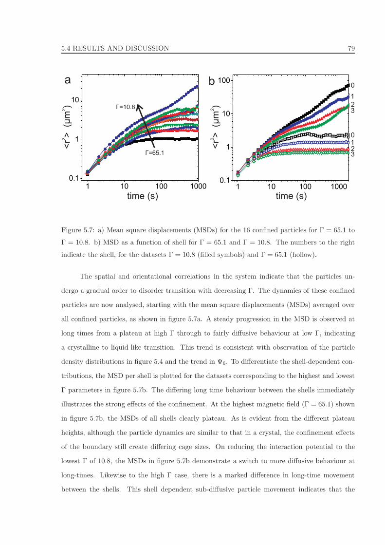
5.4 RESULTS AND DISCUSSION 79
1 10 100 10000.1
1
10
1 10 100 10000.1
1
10
100
Γ=65.1
time (s)
<r
>
(m
)2
2μ
time (s)
<r
>
(m
)2
2μ
a b 0
1
23
0123
Γ=10.8
Figure 5.7: a) Mean square displacements (MSDs) for the 16 confined particles for Γ = 65.1 to
Γ = 10.8. b) MSD as a function of shell for Γ = 65.1 and Γ = 10.8. The numbers to the right
indicate the shell, for the datasets Γ = 10.8 (filled symbols) and Γ = 65.1 (hollow).
The spatial and orientational correlations in the system indicate that the particles un-
dergo a gradual order to disorder transition with decreasing Γ. The dynamics of these confined
particles are now analysed, starting with the mean square displacements (MSDs) averaged over
all confined particles, as shown in figure 5.7a. A steady progression in the MSD is observed at
long times from a plateau at high Γ through to fairly diffusive behaviour at low Γ, indicating
a crystalline to liquid-like transition. This trend is consistent with observation of the particle
density distributions in figure 5.4 and the trend in Ψ6. To differentiate the shell-dependent con-
tributions, the MSD per shell is plotted for the datasets corresponding to the highest and lowest
Γ parameters in figure 5.7b. The differing long time behaviour between the shells immediately
illustrates the strong effects of the confinement. At the highest magnetic field (Γ = 65.1) shown
in figure 5.7b, the MSDs of all shells clearly plateau. As is evident from the different plateau
heights, although the particle dynamics are similar to that in a crystal, the confinement effects
of the boundary still create differing cage sizes. On reducing the interaction potential to the
lowest Γ of 10.8, the MSDs in figure 5.7b demonstrate a switch to more diffusive behaviour at
long-times. Likewise to the high Γ case, there is a marked difference in long-time movement
between the shells. This shell dependent sub-diffusive particle movement indicates that the
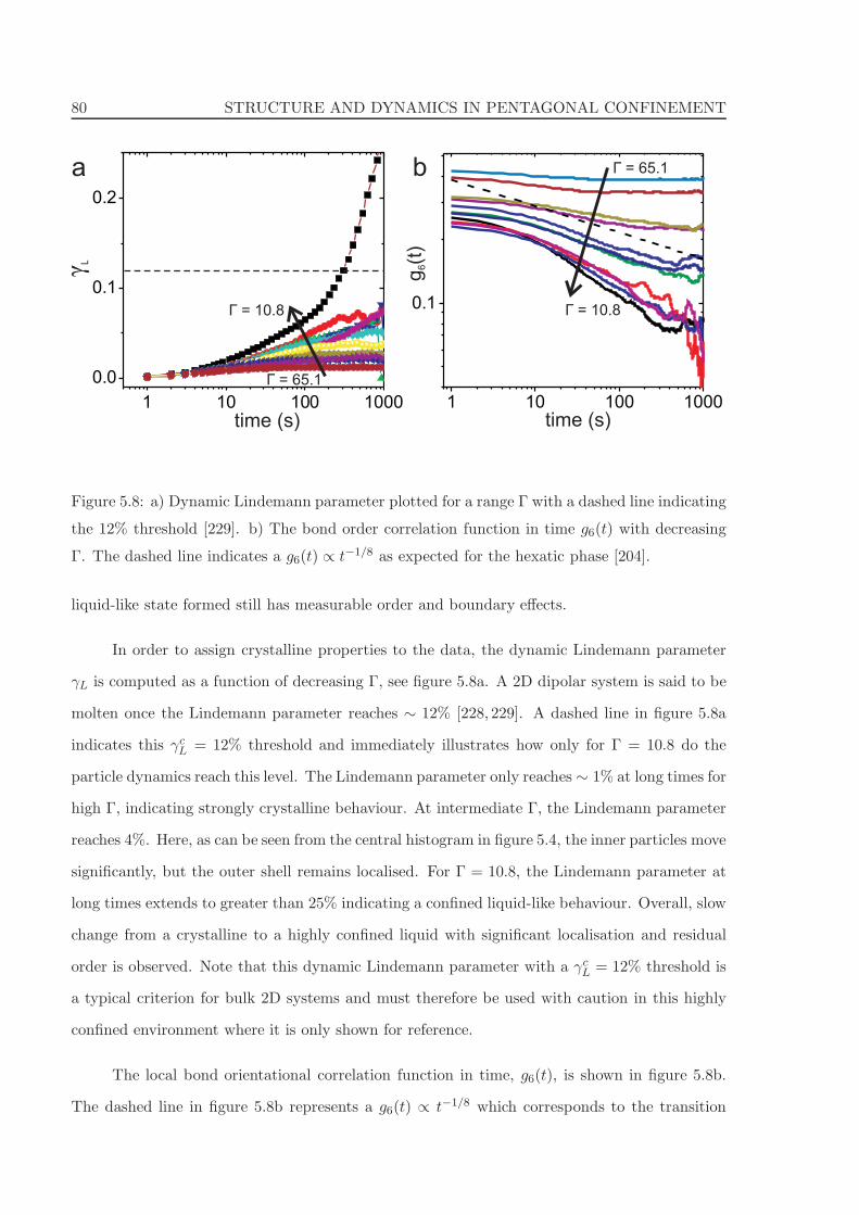
80 STRUCTURE AND DYNAMICS IN PENTAGONAL CONFINEMENT
1 10 100 1000
0.1
1 10 100 1000
0.0
0.1
0.2
Г = 10.8
Г = 65.1
time (s)time (s)g
(t)
6γL
a b
Г = 10.8
Г = 65.1
Figure 5.8: a) Dynamic Lindemann parameter plotted for a range Γ with a dashed line indicating
the 12% threshold [229]. b) The bond order correlation function in time g6(t) with decreasing
Γ. The dashed line indicates a g6(t) ∝ t−1/8 as expected for the hexatic phase [204].
liquid-like state formed still has measurable order and boundary effects.
In order to assign crystalline properties to the data, the dynamic Lindemann parameter
γL is computed as a function of decreasing Γ, see figure 5.8a. A 2D dipolar system is said to be
molten once the Lindemann parameter reaches ∼ 12% [228, 229]. A dashed line in figure 5.8a
indicates this γcL = 12% threshold and immediately illustrates how only for Γ = 10.8 do the
particle dynamics reach this level. The Lindemann parameter only reaches ∼ 1% at long times for
high Γ, indicating strongly crystalline behaviour. At intermediate Γ, the Lindemann parameter
reaches 4%. Here, as can be seen from the central histogram in figure 5.4, the inner particles move
significantly, but the outer shell remains localised. For Γ = 10.8, the Lindemann parameter at
long times extends to greater than 25% indicating a confined liquid-like behaviour. Overall, slow
change from a crystalline to a highly confined liquid with significant localisation and residual
order is observed. Note that this dynamic Lindemann parameter with a γcL = 12% threshold is
a typical criterion for bulk 2D systems and must therefore be used with caution in this highly
confined environment where it is only shown for reference.
The local bond orientational correlation function in time, g6(t), is shown in figure 5.8b.
The dashed line in figure 5.8b represents a g6(t) ∝ t−1/8 which corresponds to the transition
5.4 RESULTS AND DISCUSSION 81
from a crystalline/hexatic phase to a fluid for bulk 2D systems [230]. For the highest Γ there
is limited decay of the bond order correlation indicating crystalline behaviour. As Γ is reduced,
a weak decrease in orientational order is observed, before at the lowest Γ there is a noticeable
drop in correlation at long times. At intermediate Γ, the slope of the decay is indicative of the
g6(t) ∝ t−1/8 decay, the hexatic/solid to fluid transition. The presence of a hexatic, typified with
the presence of quasi-long range orientational and short range translation order is not relevant
in this highly confined system and so the relation is merely used as a general melting criterion.
Although the exponent decreases further as the system melts, the decay is still algebraic rather
then exponential as expected for a liquid, suggesting a more ordered liquid structure due to the
confinement.
This highly confined system of 16 particles trapped in a pentagonally shaped environment
melts from a localised crystalline-like state at ‘low temperature’ to a confined-liquid-like state
at ‘high temperature’. All the results of the analysis are consistent with this change in the
dynamics and structure of the confined particles as Γ is reduced. Reducing Γ increases the free
volume in the system permitting greater particle dynamics. Closer examination revealed how
the melting transition starts at the central particle (a disclination) and propagates outwards
as the system tries to remove this defect. The inner shells start to delocalise their positions
first, before at the lowest Γ all the shells have started to delocalise. A loss of shell-structure
dependence is indicated at the lowest Γ in Ψ6. However, as the algebraic decay in the bond
orientational correlation function indicates and the differences in the MSD between shells at
the lowest Γ illustrates, significant particle ordering is still present. These remaining boundary
effects display the highly confined nature of the system and the dynamical slowing down near
the boundary.
In contrast to the circular system studied by Bubeck et al. [197], the confining pentagonal
symmetry restricts any shell rotation. They observed a two step melting mechanism facilitated
by a shell rotation state. In contrast, the pentagonal system studied here melts with no de-
tectable differences between angular or radial mean square displacements (not shown). The
geometry frustrates the system such that complete melting cannot occur, boundary effects are
prevalent and the system is best described as a confined liquid.
82 STRUCTURE AND DYNAMICS IN PENTAGONAL CONFINEMENT
5.4.2 Particle number induced ordering behaviour
Partial melting occurs in this highly confined pentagonally shaped system when Γ is reduced via
control of an external magnetic field. Next, Γ is not controlled via the inter-particle interaction
strength, but by the number density of the confined colloidal particles. This is a problem more
akin to packing in confinement where the enforcement of an incommensurate 5-fold symmetry
on the system is expected to produce frustrated states.
As per section 5.4.1, 15 particles are tweezed to create a confining pentagon. However,
here, the number of confined particles, N , is sequentially increased from 10 to 21, whilst keeping
the magnetic field constant (2.1 mT). The interaction parameter, Γ, scales with the particle
number density via Γ ∝ ρ3
2 (see eq. (5.1)). Therefore, for simplicity the datasets are referred to
by their number of confined particles rather than Γ.
Two-dimensional histograms of the particle positions plotted over the observation time as
a function of the number of confined colloidal particles are shown in figure 5.9. The relative
amounts of particle movement appear to significantly fluctuate, revealing that the levels of pack-
ing frustration sensitively vary with the number of confined particles. The different structures
that form as the number of confined particles increases from 10 to 21 are also illustrated in the
radial histograms in figure 5.10a. The histograms are normalised such that the area under each
curve is equal to the number of confined particles in each dataset, allowing direct comparison
of the peak heights between datasets. As the number of confined particles increases, the peaks
move outwards and an extra peak is also added at 16 and 21, where a particle now occupies the
pentagon centre and a new shell is added.
Next, to give a more quantitative analysis of the packing symmetries, the orientational
bond-order parameter Ψ6 is calculated. The Ψ6 averaged over all the confined particles for each
dataset is shown in figure 5.10b, along with results from the Monte Carlo simulations. The Ψ6
fluctuates almost periodically with the number of particles. There appear to be two distinct
regimes in particle ordering behaviour: a general increase in Ψ6 from 10 to 16 particles and
quite different behaviour from 16 to 21 confined particles. The experimental and Monte Carlo
results qualitatively show very good agreement. The small systematic deviations relate to the
difficulties in mimicking the experiment, including the exact particle pair potentials and fixation
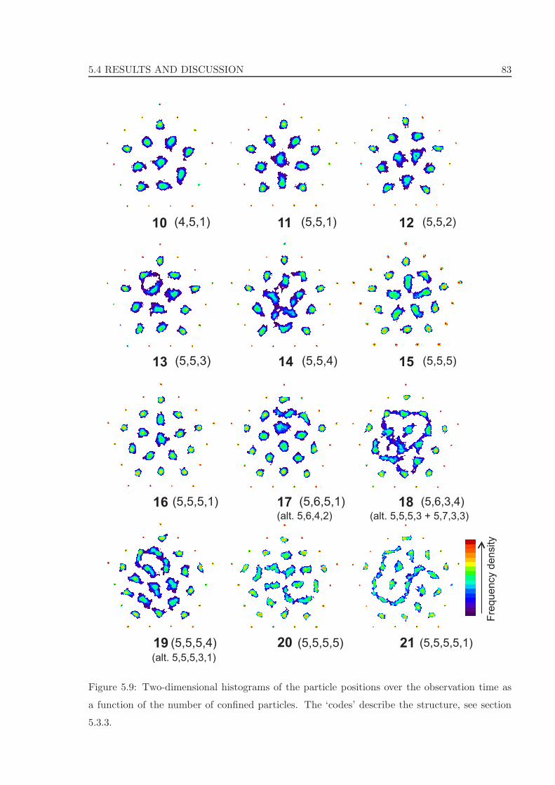
5.4 RESULTS AND DISCUSSION 83
10 11 12
16 17 18
19 20 21
Fre
quency d
ensity
(4,5,1) (5,5,1) (5,5,2)
13 14 15(5,5,3) (5,5,4) (5,5,5)
(5,5,5,1) (5,6,5,1) (5,6,3,4)
(alt. 5,5,5,3 + 5,7,3,3)
(5,5,5,4) (5,5,5,5) (5,5,5,5,1)
(alt. 5,5,5,3,1)
(alt. 5,6,4,2)
Figure 5.9: Two-dimensional histograms of the particle positions over the observation time as
a function of the number of confined particles. The ‘codes’ describe the structure, see section
5.3.3.
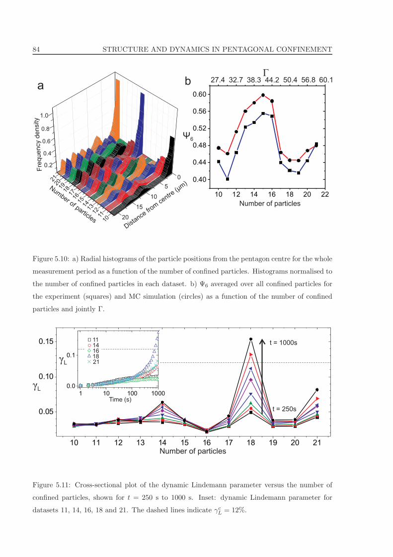
84 STRUCTURE AND DYNAMICS IN PENTAGONAL CONFINEMENT
10 12 14 16 18 20 22
0.40
0.44
0.48
0.52
0.56
0.60
Ψ6
Number of particles
Г27.4 32.7 38.3 44.2 50.4 56.8 60.1
10
0
5
15
20
20
1011
1213
1415
1817
16
1921
0.4
0.2
0.8
0.6
1.0
Distance
from
centre
(m
)μNum
ber of particles
Fre
quency
density
a b
Figure 5.10: a) Radial histograms of the particle positions from the pentagon centre for the whole
measurement period as a function of the number of confined particles. Histograms normalised to
the number of confined particles in each dataset. b) Ψ6 averaged over all confined particles for
the experiment (squares) and MC simulation (circles) as a function of the number of confined
particles and jointly Γ.
10 11 12 13 14 15 16 17 18 19 20 21
0.05
0.10
0.15 t = 1000s
t = 250s
Number of particles
γL
Time (s)
1114161821
1 10 100 1000
0.0
0.1
γL
Figure 5.11: Cross-sectional plot of the dynamic Lindemann parameter versus the number of
confined particles, shown for t = 250 s to 1000 s. Inset: dynamic Lindemann parameter for
datasets 11, 14, 16, 18 and 21. The dashed lines indicate γcL = 12%.
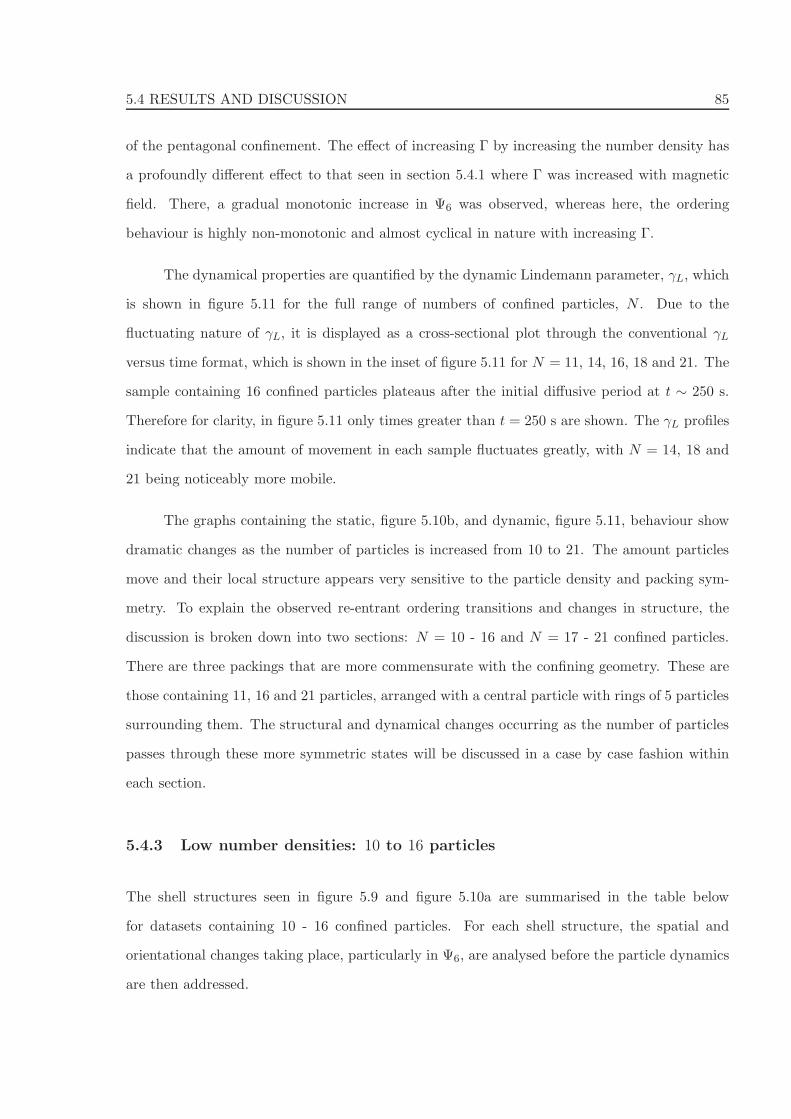
5.4 RESULTS AND DISCUSSION 85
of the pentagonal confinement. The effect of increasing Γ by increasing the number density has
a profoundly different effect to that seen in section 5.4.1 where Γ was increased with magnetic
field. There, a gradual monotonic increase in Ψ6 was observed, whereas here, the ordering
behaviour is highly non-monotonic and almost cyclical in nature with increasing Γ.
The dynamical properties are quantified by the dynamic Lindemann parameter, γL, which
is shown in figure 5.11 for the full range of numbers of confined particles, N . Due to the
fluctuating nature of γL, it is displayed as a cross-sectional plot through the conventional γL
versus time format, which is shown in the inset of figure 5.11 for N = 11, 14, 16, 18 and 21. The
sample containing 16 confined particles plateaus after the initial diffusive period at t ∼ 250 s.
Therefore for clarity, in figure 5.11 only times greater than t = 250 s are shown. The γL profiles
indicate that the amount of movement in each sample fluctuates greatly, with N = 14, 18 and
21 being noticeably more mobile.
The graphs containing the static, figure 5.10b, and dynamic, figure 5.11, behaviour show
dramatic changes as the number of particles is increased from 10 to 21. The amount particles
move and their local structure appears very sensitive to the particle density and packing sym-
metry. To explain the observed re-entrant ordering transitions and changes in structure, the
discussion is broken down into two sections: N = 10 - 16 and N = 17 - 21 confined particles.
There are three packings that are more commensurate with the confining geometry. These are
those containing 11, 16 and 21 particles, arranged with a central particle with rings of 5 particles
surrounding them. The structural and dynamical changes occurring as the number of particles
passes through these more symmetric states will be discussed in a case by case fashion within
each section.
5.4.3 Low number densities: 10 to 16 particles
The shell structures seen in figure 5.9 and figure 5.10a are summarised in the table below
for datasets containing 10 - 16 confined particles. For each shell structure, the spatial and
orientational changes taking place, particularly in Ψ6, are analysed before the particle dynamics
are then addressed.
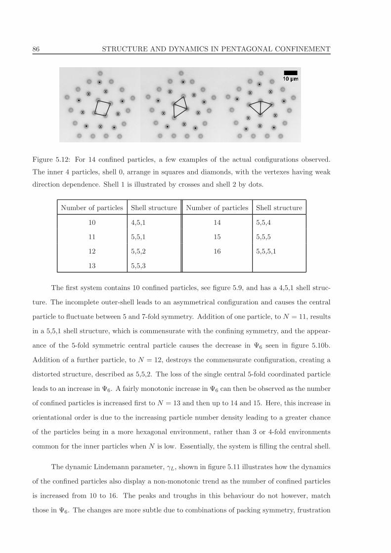
86 STRUCTURE AND DYNAMICS IN PENTAGONAL CONFINEMENT
x
x
x
x
x
x
xx
x
x
x
x
x
x
x
Figure 5.12: For 14 confined particles, a few examples of the actual configurations observed.
The inner 4 particles, shell 0, arrange in squares and diamonds, with the vertexes having weak
direction dependence. Shell 1 is illustrated by crosses and shell 2 by dots.
Number of particles Shell structure Number of particles Shell structure
10 4,5,1 14 5,5,4
11 5,5,1 15 5,5,5
12 5,5,2 16 5,5,5,1
13 5,5,3
The first system contains 10 confined particles, see figure 5.9, and has a 4,5,1 shell struc-
ture. The incomplete outer-shell leads to an asymmetrical configuration and causes the central
particle to fluctuate between 5 and 7-fold symmetry. Addition of one particle, to N = 11, results
in a 5,5,1 shell structure, which is commensurate with the confining symmetry, and the appear-
ance of the 5-fold symmetric central particle causes the decrease in Ψ6 seen in figure 5.10b.
Addition of a further particle, to N = 12, destroys the commensurate configuration, creating a
distorted structure, described as 5,5,2. The loss of the single central 5-fold coordinated particle
leads to an increase in Ψ6. A fairly monotonic increase in Ψ6 can then be observed as the number
of confined particles is increased first to N = 13 and then up to 14 and 15. Here, this increase in
orientational order is due to the increasing particle number density leading to a greater chance
of the particles being in a more hexagonal environment, rather than 3 or 4-fold environments
common for the inner particles when N is low. Essentially, the system is filling the central shell.
The dynamic Lindemann parameter, γL, shown in figure 5.11 illustrates how the dynamics
of the confined particles also display a non-monotonic trend as the number of confined particles
is increased from 10 to 16. The peaks and troughs in this behaviour do not however, match
those in Ψ6. The changes are more subtle due to combinations of packing symmetry, frustration
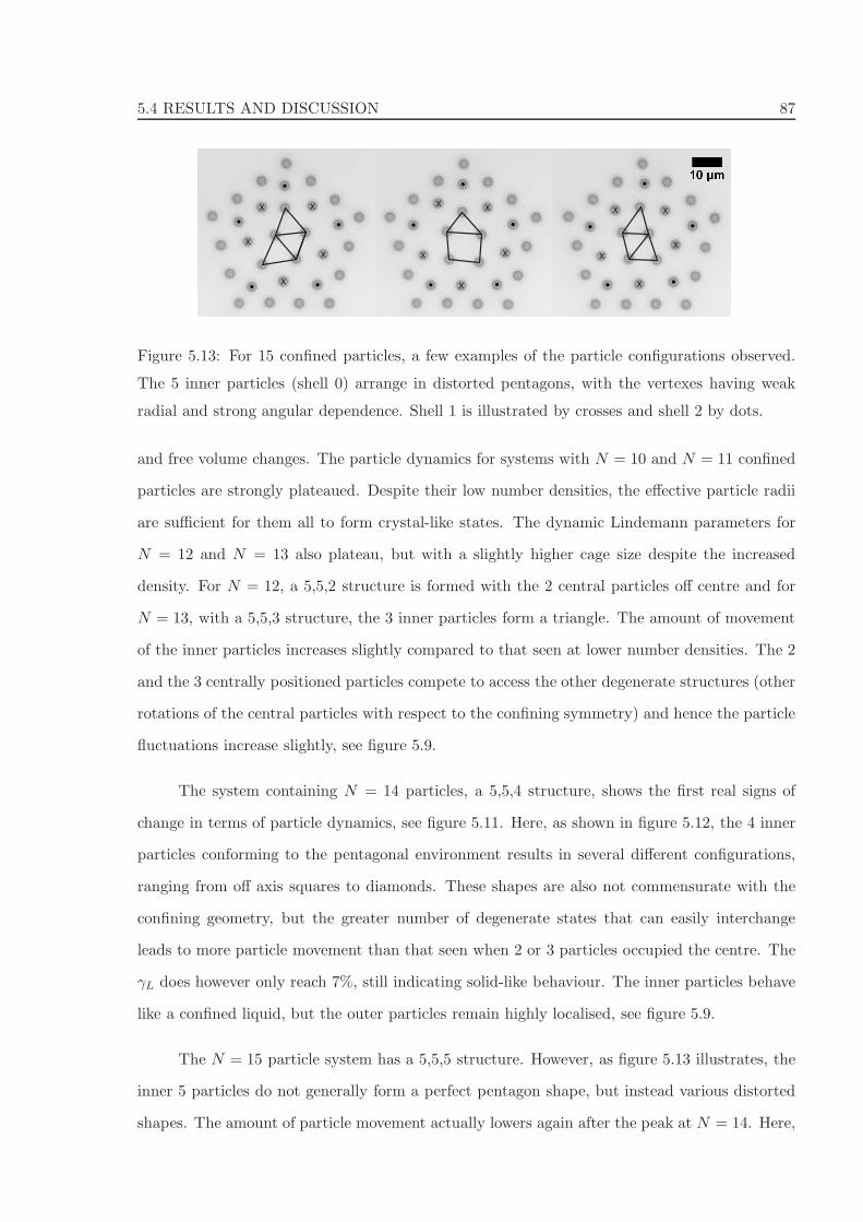
5.4 RESULTS AND DISCUSSION 87
x x
x
x
x
xx
x x
x
x
x
x
x
x
Figure 5.13: For 15 confined particles, a few examples of the particle configurations observed.
The 5 inner particles (shell 0) arrange in distorted pentagons, with the vertexes having weak
radial and strong angular dependence. Shell 1 is illustrated by crosses and shell 2 by dots.
and free volume changes. The particle dynamics for systems with N = 10 and N = 11 confined
particles are strongly plateaued. Despite their low number densities, the effective particle radii
are sufficient for them all to form crystal-like states. The dynamic Lindemann parameters for
N = 12 and N = 13 also plateau, but with a slightly higher cage size despite the increased
density. For N = 12, a 5,5,2 structure is formed with the 2 central particles off centre and for
N = 13, with a 5,5,3 structure, the 3 inner particles form a triangle. The amount of movement
of the inner particles increases slightly compared to that seen at lower number densities. The 2
and the 3 centrally positioned particles compete to access the other degenerate structures (other
rotations of the central particles with respect to the confining symmetry) and hence the particle
fluctuations increase slightly, see figure 5.9.
The system containing N = 14 particles, a 5,5,4 structure, shows the first real signs of
change in terms of particle dynamics, see figure 5.11. Here, as shown in figure 5.12, the 4 inner
particles conforming to the pentagonal environment results in several different configurations,
ranging from off axis squares to diamonds. These shapes are also not commensurate with the
confining geometry, but the greater number of degenerate states that can easily interchange
leads to more particle movement than that seen when 2 or 3 particles occupied the centre. The
γL does however only reach 7%, still indicating solid-like behaviour. The inner particles behave
like a confined liquid, but the outer particles remain highly localised, see figure 5.9.
The N = 15 particle system has a 5,5,5 structure. However, as figure 5.13 illustrates, the
inner 5 particles do not generally form a perfect pentagon shape, but instead various distorted
shapes. The amount of particle movement actually lowers again after the peak at N = 14. Here,
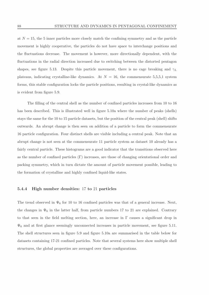
88 STRUCTURE AND DYNAMICS IN PENTAGONAL CONFINEMENT
at N = 15, the 5 inner particles more closely match the confining symmetry and as the particle
movement is highly cooperative, the particles do not have space to interchange positions and
the fluctuations decrease. The movement is however, more directionally dependent, with the
fluctuations in the radial direction increased due to switching between the distorted pentagon
shapes, see figure 5.13. Despite this particle movement, there is no cage breaking and γL
plateaus, indicating crystalline-like dynamics. At N = 16, the commensurate 5,5,5,1 system
forms, this stable configuration locks the particle positions, resulting in crystal-like dynamics as
is evident from figure 5.9.
The filling of the central shell as the number of confined particles increases from 10 to 16
has been described. This is illustrated well in figure 5.10a where the number of peaks (shells)
stays the same for the 10 to 15 particle datasets, but the position of the central peak (shell) shifts
outwards. An abrupt change is then seen on addition of a particle to form the commensurate
16 particle configuration. Four distinct shells are visible including a central peak. Note that an
abrupt change is not seen at the commensurate 11 particle system as dataset 10 already has a
fairly central particle. These histograms are a good indicator that the transitions observed here
as the number of confined particles (Γ) increases, are those of changing orientational order and
packing symmetry, which in turn dictate the amount of particle movement possible, leading to
the formation of crystalline and highly confined liquid-like states.
5.4.4 High number densities: 17 to 21 particles
The trend observed in Ψ6 for 10 to 16 confined particles was that of a general increase. Next,
the changes in Ψ6 in the latter half, from particle numbers 17 to 21 are explained. Contrary
to that seen in the field melting section, here, an increase in Γ causes a significant drop in
Ψ6 and at first glance seemingly unconnected increases in particle movement, see figure 5.11.
The shell structures seen in figure 5.9 and figure 5.10a are summarised in the table below for
datasets containing 17-21 confined particles. Note that several systems here show multiple shell
structures, the global properties are averaged over these configurations.
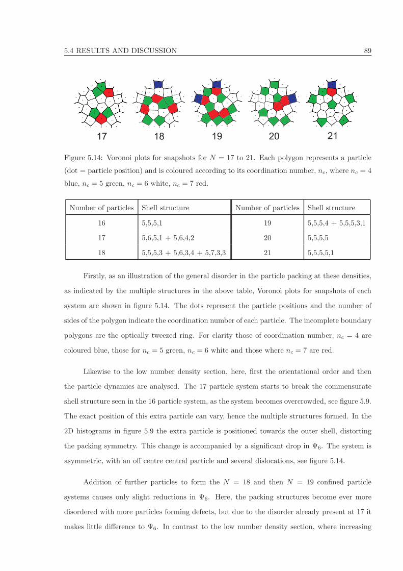
5.4 RESULTS AND DISCUSSION 89
17 18 19 20 21
Figure 5.14: Voronoi plots for snapshots for N = 17 to 21. Each polygon represents a particle
(dot = particle position) and is coloured according to its coordination number, nc, where nc = 4
blue, nc = 5 green, nc = 6 white, nc = 7 red.
Number of particles Shell structure Number of particles Shell structure
16 5,5,5,1 19 5,5,5,4 + 5,5,5,3,1
17 5,6,5,1 + 5,6,4,2 20 5,5,5,5
18 5,5,5,3 + 5,6,3,4 + 5,7,3,3 21 5,5,5,5,1
Firstly, as an illustration of the general disorder in the particle packing at these densities,
as indicated by the multiple structures in the above table, Voronoi plots for snapshots of each
system are shown in figure 5.14. The dots represent the particle positions and the number of
sides of the polygon indicate the coordination number of each particle. The incomplete boundary
polygons are the optically tweezed ring. For clarity those of coordination number, nc = 4 are
coloured blue, those for nc = 5 green, nc = 6 white and those where nc = 7 are red.
Likewise to the low number density section, here, first the orientational order and then
the particle dynamics are analysed. The 17 particle system starts to break the commensurate
shell structure seen in the 16 particle system, as the system becomes overcrowded, see figure 5.9.
The exact position of this extra particle can vary, hence the multiple structures formed. In the
2D histograms in figure 5.9 the extra particle is positioned towards the outer shell, distorting
the packing symmetry. This change is accompanied by a significant drop in Ψ6. The system is
asymmetric, with an off centre central particle and several dislocations, see figure 5.14.
Addition of further particles to form the N = 18 and then N = 19 confined particle
systems causes only slight reductions in Ψ6. Here, the packing structures become ever more
disordered with more particles forming defects, but due to the disorder already present at 17 it
makes little difference to Ψ6. In contrast to the low number density section, where increasing
90 STRUCTURE AND DYNAMICS IN PENTAGONAL CONFINEMENT
the number of particles generally increased Ψ6 and the number of 6-fold environments, here,
Ψ6 generally decreases due to the fact that the system contains more than the commensurate
N = 16 particles. Hence, the increased packing fraction forces more particles into 4, 5 and 7-fold
environments, particularly the 4-fold corner sites, see figure 5.14.
A slight increase in Ψ6 is actually observed on formation of the N = 20 particle system.
Despite the added particle, the symmetry of the system increases due to a 5,5,5,5 shell structure
forming with a vacancy at the centre. This central hole is then filled on addition to form the
21 particle system, a 5,5,5,5,1 structure, which is commensurate with the confining geometry
and is accompanied by a further increase in Ψ6. Unlike the earlier transitions to commensurate
states (the shifts from N = 10 → 11 and N = 15 → 16), here Ψ6 increases on filling the central
hole. Despite forming a 5-fold disclination at the centre, this ordering effect increases Ψ6 in the
outer shells sufficiently to create an overall increase.
In terms of particle movement, as indicated by the dynamic Lindemann parameter in
figure 5.11, the dynamics are variable and not coherent with Ψ6. For the 17 particle system,
the particle dynamics are greater than the 16 particle system, but are still fairly plateaued. The
most dramatic change in particle dynamics occurs on addition to 18 particles. Here, γL , as
shown in figure 5.11 demonstrates that the particle dynamics are liquid-like and indicative of
melting, easily breaching the 12% threshold expected for melting in 2D dipolar systems [229].
However, the particle movements are also strongly heterogeneous, chains of cooperatively moving
particles, constituting the ‘molten’ particles, move between the remaining highly static particles.
This increased particle movement is consistent with the many different shell structures observed,
see the table above, just one is illustrated in figure 5.9.
An equally abrupt change in system properties occurs on addition to N = 19 particles,
here, the particle dynamics shift from liquid-like to crystalline. The particles become jammed
and more localised due to the high number density in the system. Such a large change in particle
mobility on addition of one particle is remarkable and illustrates the subtleties of the system.
The particle density and symmetry at this packing density are not favourable for chains of
cooperatively moving particles to form.
5.4 RESULTS AND DISCUSSION 91
Although Ψ6 changes noticeably between 19 and 20, no change in particle dynamics is
observed on forming the 20 particle system. The dynamics are strongly crystalline, and as the
1D and 2D histograms illustrate, see figure 5.9 and figure 5.10a, the particles are highly localised
despite their lack of orientational order. On formation of the commensurate 21 particle system
an increase in the particle dynamics is observed. Although not as abrupt as the change at
N = 18, the mobility increases to γL ∼ 9% at long times, despite the increased number density.
This sub-diffusive behaviour is against the trend seen in the other commensurate configurations,
N = 11 and N = 16, who demonstrate strongly crystalline dynamics. It is hypothesised that
this mobility increase is due to the higher symmetry helping to unjam the system.
Due to the highly frustrated nature and the long time scales involved in the systems
containing high numbers of confined particles, Monte Carlo (MC) simulations were performed
to compare with the experimental particle density distributions. The experimental and MC
simulation results qualitatively show excellent agreement in the terms of the orientation order
parameter Ψ6, as shown in figure 5.10b. The small differences arise due to difficulty in matching
the 1/r3 potential between the experiment and simulation and the fixing of the pentagonal array.
The 2D histograms for the MC simulations for datasets with 16 to 21 confined particles
are shown in figure 5.15. The simulation is far more efficient at sampling phase space than the
experiment. To enable a better comparison with the simulation the sampling of the experiment
is artificially increased by computing all the symmetry operations, for all the particle positions,
over all time. Given the 5-fold rotational and the 5 reflection symmetry axes present in the
system, and setting the pentagon centre as the reference, the colloidal particle positions over the
experimental run are rotated and reflected 5 times each. The ‘equilibrium’ histograms of the
experimental data are shown in figure 5.15 along side the MC histograms. The 2D histograms
of the particle coordinates from the MC simulation are in good agreement to the symmetry
adjusted experimental data for all the number densities shown in figure 5.15. The peaks and
troughs in intensity all lie at the same positions around the pentagon. This illustrates that
although not all the configurations are sampled within the duration of the experiment it is
consistent with the ‘equilibrium’ behaviour of the simulations.
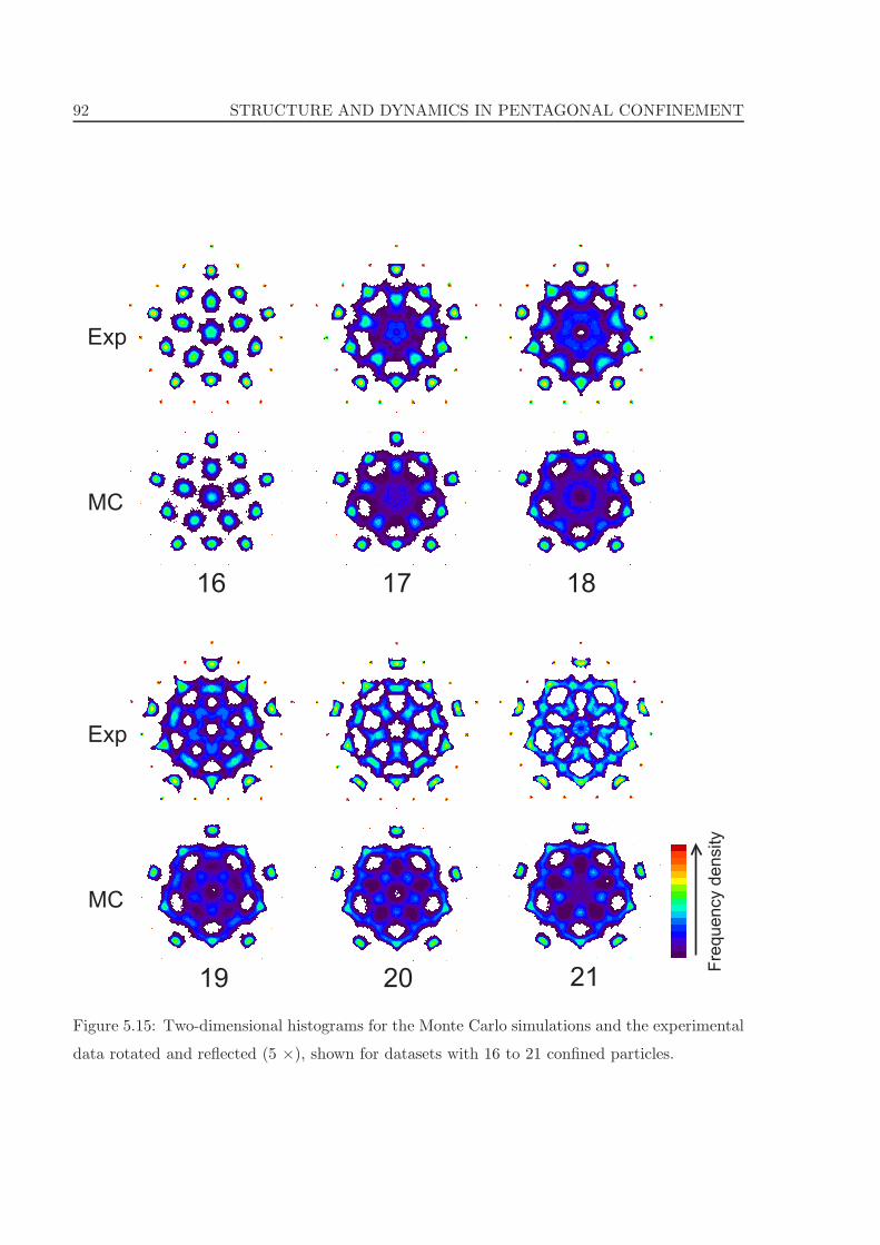
92 STRUCTURE AND DYNAMICS IN PENTAGONAL CONFINEMENT
17 18
19 20 21
Fre
qu
en
cy d
en
sity
16
Exp
MC
Exp
MC
Figure 5.15: Two-dimensional histograms for the Monte Carlo simulations and the experimental
data rotated and reflected (5 ×), shown for datasets with 16 to 21 confined particles.
5.5 CONCLUSIONS 93
5.5 Conclusions
The structure and dynamics of particles confined in a pentagonal environment have been studied.
The state of the system is characterised by Γ which depends on both the magnetic field and the
particle number density. Both these pathways were probed to alter Γ and in doing so displayed
quite contrasting results. In the field melting section, the behaviour of the commensurate 16
particle system was studied as a function of decreasing interaction parameter, Γ. At the highest
Γ, the confined particles were highly localised and the state described as crystal-like owing
to the lack of hexagonal symmetry and the central disclination. On lowering Γ, the melting
transition started at the central disclination and propagated outwards. The dynamics of the
confined particles at low Γ were clearly liquid-like, even for the most localised particles. However,
observation of the 1D and 2D histograms illustrated the clear shell behaviour still present in
the system. Hence, the structures formed from melting the crystal-like state were referred
to as a confined liquid, where the boundary effects prevented a complete loss of environment
dependence.
In the second section, Γ was increased via particle density rather than decreased through
magnetic field. The dynamic and structural behaviour displayed almost cyclical properties as
the number of confined particles was increased from N = 10 to N = 21. The orientational
order parameter, Ψ6, was seen to increase with particle number up until N = 15 particles, in a
similar fashion to that seen in the field melting behaviour. However, on increase to 16 particles
and beyond, a general decrease in Ψ6 was observed before a final increase again at 21 particles.
This almost periodic re-entrant ordering behaviour is a result of the pentagonal environment
where the level of packing frustration and symmetry is highly dependent on the number of
particles. Parallel to the orientation effects, the dynamics of the confined particles fluctuated
with a pattern incommensurate to the oscillation in Ψ6. The cross-sectional plot through the
dynamic Lindemann parameter, see figure 5.11, displayed this variable particle mobility and
therefore serves as a useful ‘state diagram’ for the mobility as a function of number density.
The symmetry and orientational order in the packing arrangements affects in turn the particle
dynamics, the system is therefore highly sensitive to the number of confined particles. Notable
94 STRUCTURE AND DYNAMICS IN PENTAGONAL CONFINEMENT
effects included a rapid increase in particle mobility at 18 particles due to the system trying to
access the different degenerate particle configurations. This dynamic behaviour disappeared at
19 particles despite no change in Ψ6.
Acknowledgments
This work was done in collaboration with Henry Martin and Dirk Aarts. Roland Roth is thanked
for useful discussions.

Chapter 6
Particle dynamics in random
confinement
ABSTRACT
The behaviour of a two-dimensional (2D) colloidal fluid confined within a random matrix of
obstacles is studied using optical microscopy. A binary mixture of colloidal particles is confined
in 2D such that the large particles become fixed whilst the small particles remain mobile. The
large static particles form the confining random matrix around which the small particles, the
fluid, are able to move. Both the large and small colloidal particle have super-paramagnetic
properties, allowing the inter-particle potential and hence the effective area fraction of the fluid
and the matrix to be controlled with an external magnetic field. The state diagram of the
effective area fraction of the matrix versus that of the fluid particles is mapped out using the
Barker-Henderson formalism. Starting from different number densities of the matrix and fluid
particles, the external magnetic field is increased to scan across the state diagram. At each state
point, the particle dynamics are studied. Good agreement is found with both simulation and
theory, with a slowing down of the dynamics of the fluid particles characteristic of the onset of
a type B glass transition observed at low matrix density and a localisation-diffusion dominated
type A glass transition at high matrix density.
95

96 PARTICLE DYNAMICS IN RANDOM CONFINEMENT
6.1 Introduction
The movement of fluids through porous media is of significance to many fields, including the
pharmaceutical, oil and gas industries. Materials containing pores are widely used as filters for
molecular sieves [235,236] and as catalysts [33]. The transport of liquids through soil and rock
formations is important for oil and gas extraction and for the removal of pollutants. Improved
knowledge of the effects of confinement on the diffusion and absorption of liquids in these porous
materials is key to improving performance in these industries. In addition, the phase behaviour
of fluids is well known to differ in confinement [188, 189] and is of vital importance to the
geological processes of frost heaving and freeze thaw weathering [237]. Liquids confined in
porous matrices also have similarities to the percolation networks [238] formed in the jamming
transition of granular materials [239]. In particular, the effects on fluid behaviour of both
porous and planar confinement have been well documented, with observations of both increases
and decreases in the glass transition temperature [154, 240, 241]. These studies are however,
performed in porous glasses [242] where systematically controlling and varying the pore size
and connectivity is difficult. Hence, for systematic particle level studies over many matrix
configurations, simulation and theory provide a useful pathway for characterising these systems.
The simplest model for describing transport in heterogeneous media is the Lorentz model
[36,243]. Here, a single tracer particle (a ‘fluid’ particle) explores a randomly distributed array
of fixed overlapping obstacles (the ‘matrix’ particles). A theoretical formalism was then put
forward by Krakoviack in 2005 [34, 244] who used mode coupling theory to study a Lorentz
model-based system, with variable fluid and matrix densities, to describe the dynamics of fluids
in random porous matrices. The results of this theoretical framework were then tested by
a number of molecular dynamics simulation studies of hard sphere fluids confined in porous
matrices by Kurzidim et al. [35, 245, 246] and Kim et al. [247]. The aim in this chapter is to
systematically analyse in experiment, the effect of a confining array of fixed colloidal particles,
the ‘matrix’, on the dynamics of free colloidal particles acting as the ‘fluid’. This study provides
a direct comparison to the simulation studies, through analysis of the single particle dynamics
of the confined fluid.

6.2 BACKGROUND 97
6.2 Background
6.2.1 Glass transitions in confinement
When a liquid is cooled below its melting temperature without it freezing, it is defined as
supercooled. As the liquid is cooled further, the particle dynamics slow down, the viscosity
increases, and the structure approaches an arrest scenario [153]. This bypassing of the freezing
transition eventually results in an amorphous metastable state known as a glass. The dynamical
slowing down is characterised by an increase in the fluid relaxation time, the characteristic
timescale over which a system returns to equilibrium after a perturbation. The glass transition
temperature is defined in molecular systems by a viscosity of 1012 Pa s [154, 248]. This great
increase in viscosity and in relaxation times occurs despite only a small change in structure. A
characteristic feature of supercooled liquids approaching the glass transition is the formation and
growth of dynamical heterogeneities and cooperatively rearranging regions in the liquid [142,156].
Phase changes are well known to differ under confinement, for instance freezing point
depression in small pores [188–190], and see chapter 5. The glass transition temperature has
also been shown to shift under confinement with reports of a reduction in the glass transition
temperature in liquids confined in nanometer size pores [249]. The glass transition is synonymous
with increasing time and length scales of particle relaxation. When the length-scales of the
porous confinement approaches or becomes smaller than these intrinsic length scales, finite
size effects are expected to impact on the glass transition [250, 251]. By reverse argument,
observing at what confinement size the glass transition is altered gives an indication of the size
of cooperative length scales in the supercooled liquid [252].
The effect of porous confinement on the glass transition is far from clear [154, 240]. The
glass transition temperature has been determined experimentally for many different materials
within differing porous confinement. However, the transition temperature has been seen to both
increase and decrease with respect to the transition in the bulk [241,253–256]. Observations have
been made of the same liquid producing differing directions of change in the glass transition,
whilst in different material confinement [248]. Furthermore, these experimental studies cannot
easily access the single particle dynamics or systematically assess a wide range of pore structures.
98 PARTICLE DYNAMICS IN RANDOM CONFINEMENT
These difficulties have therefore provoked further interest in theoretical and simulation studies
of the dynamics of fluids in random confinement, starting with the Lorentz model, these are now
discussed.
6.2.2 Theoretical and simulation predictions for fluids in random media
The Lorentz model represents a method for describing transport in heterogeneous media where
a single tracer particle explores a randomly distributed array of fixed hard-core obstacles [36,
257]. The obstacles are distributed such that they may overlap forming clusters and trap the
tracer particle in voids. At low obstacle densities the tracer particle is able to diffuse normally
throughout the percolating network of voids. However, as the obstacle density is increased, at
a certain threshold, the voids no longer percolate the whole system and a percolation transition
occurs [238]. The tracer particle experiences a localisation transition, where at this critical
density and above, the tracer particle is always trapped in the disconnected voids between the
obstacles. The localisation transition is characterised by a continuous decay in the dynamic
correlators and anomalous sub-diffusive behaviour at long times [247,258], see figure 6.2.
Until recently, there had been less extensive work on any theoretical or simulation studies
to investigate systems containing multiple interacting tracer particles. Mode coupling theory
(MCT) has been successfully employed to predict many aspects of the slowing down of structural
relaxation that occurs on cooling towards the glass transition [259,260]. An extension to mode
coupling theory was made by Krakoviack [34] in 2005 where he applied MCT to study the
dynamics of fluids confined in porous matrices, using the quenched-annealed (QA) formalism. As
the name suggests, this method of creating the random porous matrix involves first equilibrating
the positions of the matrix particles within the system, quenching them to form a static matrix,
before finally the fluid particles are inserted and equilibrated.
A schematic of the liquid-glass state diagram of a 3D hard sphere system predicted by this
extension to MCT is shown in figure 6.1. Here, the volume fraction of the fluid particles, φF , is
mapped out versus the volume fraction of the matrix particles, φM . The theory predicts many
interesting features including two types of glass transition and a re-entrant glass transition at
high φM . A ‘type B glass transition’ is expected at low φM and high φF and is that seen com-
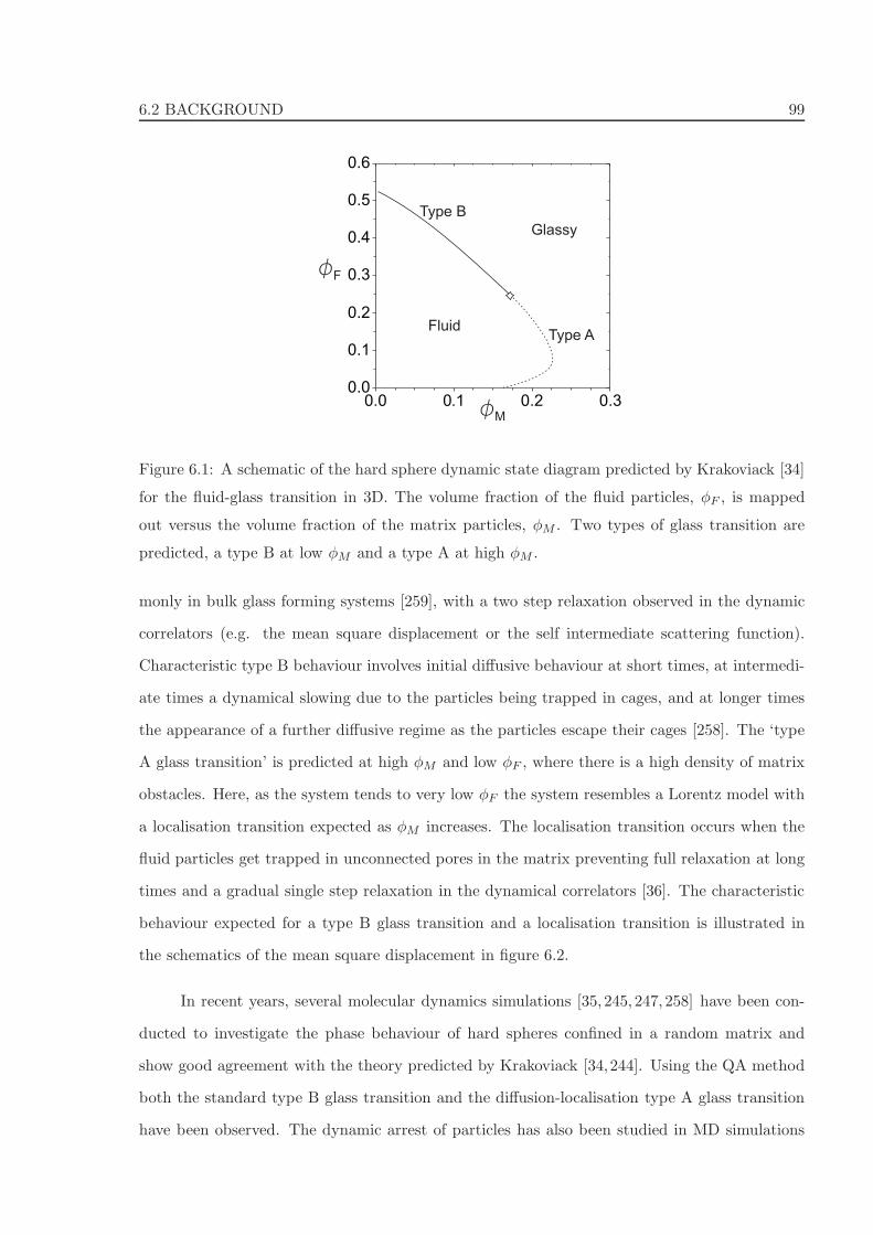
6.2 BACKGROUND 99
0.0 0.1 0.2 0.30.0
0.1
0.2
0.3
0.4
0.5
0.6
Fluid
Glassy
fM
fF
Type B
Type A
Figure 6.1: A schematic of the hard sphere dynamic state diagram predicted by Krakoviack [34]
for the fluid-glass transition in 3D. The volume fraction of the fluid particles, φF , is mapped
out versus the volume fraction of the matrix particles, φM . Two types of glass transition are
predicted, a type B at low φM and a type A at high φM .
monly in bulk glass forming systems [259], with a two step relaxation observed in the dynamic
correlators (e.g. the mean square displacement or the self intermediate scattering function).
Characteristic type B behaviour involves initial diffusive behaviour at short times, at intermedi-
ate times a dynamical slowing due to the particles being trapped in cages, and at longer times
the appearance of a further diffusive regime as the particles escape their cages [258]. The ‘type
A glass transition’ is predicted at high φM and low φF , where there is a high density of matrix
obstacles. Here, as the system tends to very low φF the system resembles a Lorentz model with
a localisation transition expected as φM increases. The localisation transition occurs when the
fluid particles get trapped in unconnected pores in the matrix preventing full relaxation at long
times and a gradual single step relaxation in the dynamical correlators [36]. The characteristic
behaviour expected for a type B glass transition and a localisation transition is illustrated in
the schematics of the mean square displacement in figure 6.2.
In recent years, several molecular dynamics simulations [35, 245, 247, 258] have been con-
ducted to investigate the phase behaviour of hard spheres confined in a random matrix and
show good agreement with the theory predicted by Krakoviack [34,244]. Using the QA method
both the standard type B glass transition and the diffusion-localisation type A glass transition
have been observed. The dynamic arrest of particles has also been studied in MD simulations
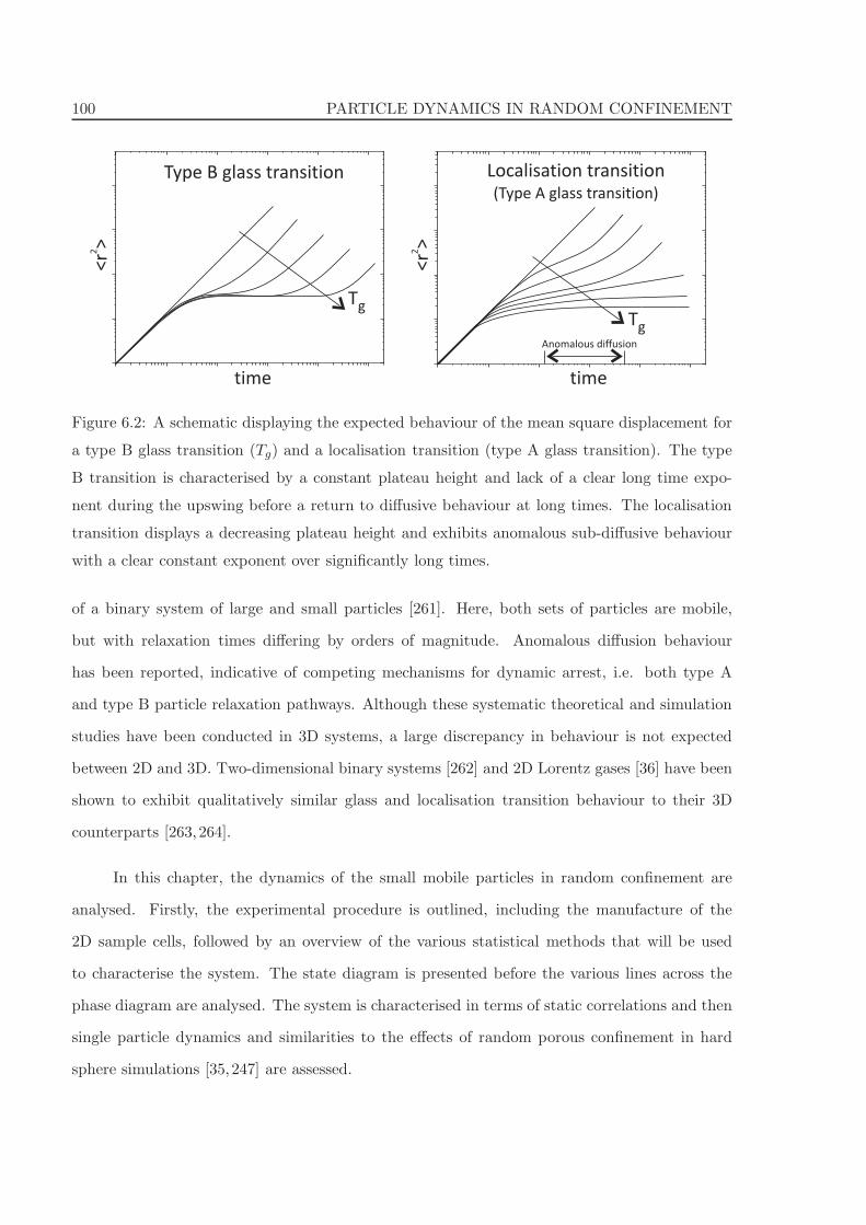
100 PARTICLE DYNAMICS IN RANDOM CONFINEMENT
timetime
<r
>2
<r
>2
TgTg
Type B glass transition Localisation transition(Type A glass transition)
Anomalous diffusion
Figure 6.2: A schematic displaying the expected behaviour of the mean square displacement for
a type B glass transition (Tg) and a localisation transition (type A glass transition). The type
B transition is characterised by a constant plateau height and lack of a clear long time expo-
nent during the upswing before a return to diffusive behaviour at long times. The localisation
transition displays a decreasing plateau height and exhibits anomalous sub-diffusive behaviour
with a clear constant exponent over significantly long times.
of a binary system of large and small particles [261]. Here, both sets of particles are mobile,
but with relaxation times differing by orders of magnitude. Anomalous diffusion behaviour
has been reported, indicative of competing mechanisms for dynamic arrest, i.e. both type A
and type B particle relaxation pathways. Although these systematic theoretical and simulation
studies have been conducted in 3D systems, a large discrepancy in behaviour is not expected
between 2D and 3D. Two-dimensional binary systems [262] and 2D Lorentz gases [36] have been
shown to exhibit qualitatively similar glass and localisation transition behaviour to their 3D
counterparts [263,264].
In this chapter, the dynamics of the small mobile particles in random confinement are
analysed. Firstly, the experimental procedure is outlined, including the manufacture of the
2D sample cells, followed by an overview of the various statistical methods that will be used
to characterise the system. The state diagram is presented before the various lines across the
phase diagram are analysed. The system is characterised in terms of static correlations and then
single particle dynamics and similarities to the effects of random porous confinement in hard
sphere simulations [35,247] are assessed.
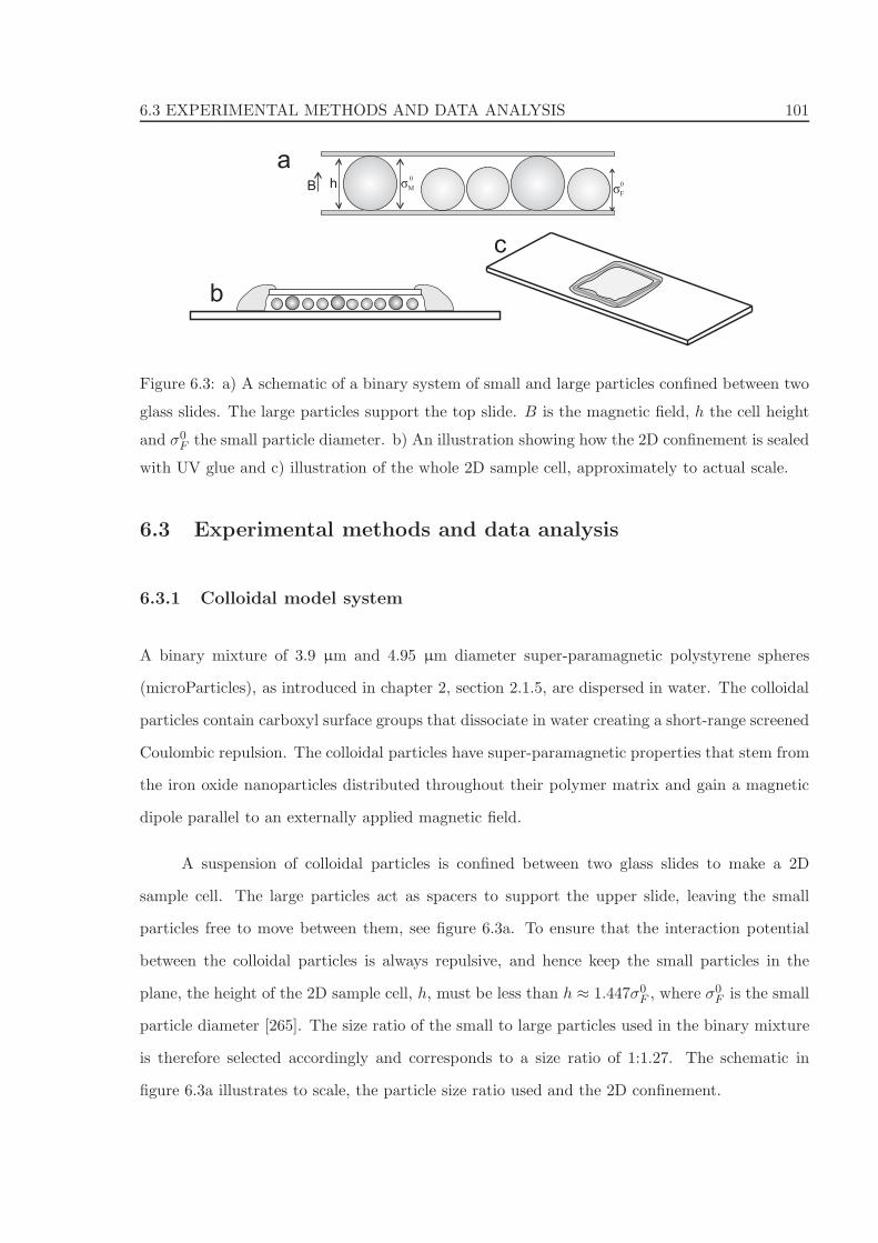
6.3 EXPERIMENTAL METHODS AND DATA ANALYSIS 101
hB σF
0σM
0
a
b
c
Figure 6.3: a) A schematic of a binary system of small and large particles confined between two
glass slides. The large particles support the top slide. B is the magnetic field, h the cell height
and σ0F the small particle diameter. b) An illustration showing how the 2D confinement is sealed
with UV glue and c) illustration of the whole 2D sample cell, approximately to actual scale.
6.3 Experimental methods and data analysis
6.3.1 Colloidal model system
A binary mixture of 3.9 µm and 4.95 µm diameter super-paramagnetic polystyrene spheres
(microParticles), as introduced in chapter 2, section 2.1.5, are dispersed in water. The colloidal
particles contain carboxyl surface groups that dissociate in water creating a short-range screened
Coulombic repulsion. The colloidal particles have super-paramagnetic properties that stem from
the iron oxide nanoparticles distributed throughout their polymer matrix and gain a magnetic
dipole parallel to an externally applied magnetic field.
A suspension of colloidal particles is confined between two glass slides to make a 2D
sample cell. The large particles act as spacers to support the upper slide, leaving the small
particles free to move between them, see figure 6.3a. To ensure that the interaction potential
between the colloidal particles is always repulsive, and hence keep the small particles in the
plane, the height of the 2D sample cell, h, must be less than h ≈ 1.447σ0F , where σ
0F is the small
particle diameter [265]. The size ratio of the small to large particles used in the binary mixture
is therefore selected accordingly and corresponds to a size ratio of 1:1.27. The schematic in
figure 6.3a illustrates to scale, the particle size ratio used and the 2D confinement.
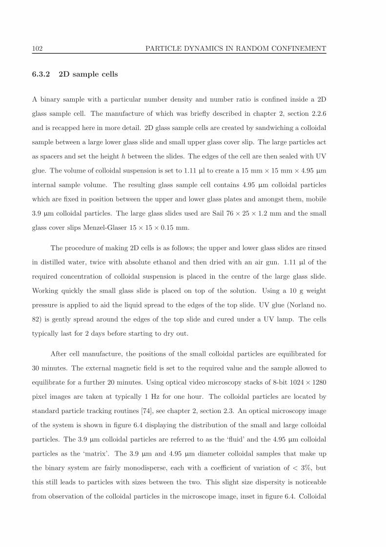
102 PARTICLE DYNAMICS IN RANDOM CONFINEMENT
6.3.2 2D sample cells
A binary sample with a particular number density and number ratio is confined inside a 2D
glass sample cell. The manufacture of which was briefly described in chapter 2, section 2.2.6
and is recapped here in more detail. 2D glass sample cells are created by sandwiching a colloidal
sample between a large lower glass slide and small upper glass cover slip. The large particles act
as spacers and set the height h between the slides. The edges of the cell are then sealed with UV
glue. The volume of colloidal suspension is set to 1.11 µl to create a 15 mm× 15 mm× 4.95 µm
internal sample volume. The resulting glass sample cell contains 4.95 µm colloidal particles
which are fixed in position between the upper and lower glass plates and amongst them, mobile
3.9 µm colloidal particles. The large glass slides used are Sail 76 × 25 × 1.2 mm and the small
glass cover slips Menzel-Glaser 15× 15× 0.15 mm.
The procedure of making 2D cells is as follows; the upper and lower glass slides are rinsed
in distilled water, twice with absolute ethanol and then dried with an air gun. 1.11 µl of the
required concentration of colloidal suspension is placed in the centre of the large glass slide.
Working quickly the small glass slide is placed on top of the solution. Using a 10 g weight
pressure is applied to aid the liquid spread to the edges of the top slide. UV glue (Norland no.
82) is gently spread around the edges of the top slide and cured under a UV lamp. The cells
typically last for 2 days before starting to dry out.
After cell manufacture, the positions of the small colloidal particles are equilibrated for
30 minutes. The external magnetic field is set to the required value and the sample allowed to
equilibrate for a further 20 minutes. Using optical video microscopy stacks of 8-bit 1024× 1280
pixel images are taken at typically 1 Hz for one hour. The colloidal particles are located by
standard particle tracking routines [74], see chapter 2, section 2.3. An optical microscopy image
of the system is shown in figure 6.4 displaying the distribution of the small and large colloidal
particles. The 3.9 µm colloidal particles are referred to as the ‘fluid’ and the 4.95 µm colloidal
particles as the ‘matrix’. The 3.9 µm and 4.95 µm diameter colloidal samples that make up
the binary system are fairly monodisperse, each with a coefficient of variation of < 3%, but
this still leads to particles with sizes between the two. This slight size dispersity is noticeable
from observation of the colloidal particles in the microscope image, inset in figure 6.4. Colloidal
6.3 EXPERIMENTAL METHODS AND DATA ANALYSIS 103
particles are reclassified as fluid or matrix according to their mobility where required. This
concerns only a very small fraction of the particles. Any drift in the colloidal particle positions
due to temperature fluctuations in the microscope are corrected for with respect to the fixed
4.95 µm particles. This leads to the coordinates of both the 3.9 µm (fluid) and the 4.95 µm
(matrix) colloidal particles being found for each time frame.
6.3.3 Mapping to packing fractions
The inter-particle interaction potential of the super-paramagnetic colloidal particles is controlled
via an external magnetic field. In order to calculate the effective packing fraction for the colloidal
particles with these soft repulsions, an effective hard sphere particle diameter is calculated using
a Barker-Henderson like approach [169, 266, 267]. The soft 1r3 potential is mapped onto that of
an effective hard sphere diameter σeff
as a function of the applied magnetic field according to:
σeff
= σ0 +
∫ ∞
σ0
(1− e−βU(r))dr (6.1)
where σ0 is the original hard sphere diameter and β = 1/kBT . The interaction potential, U(r),
is given by U(r) = µ0χ2B2
4πr3for two parallel magnetic dipoles separated by a distance r and where
µ0 is the permeability of free space and χ the magnetic susceptibility of the colloidal particle,
see eq. (2.5) in chapter 2.
In combination, manipulation of both the colloidal particle density and the effective hard
sphere diameter allows the state diagram of the area fraction of the large versus the area fraction
of the small colloidal particles to be mapped out. This enables one sample cell, which contains
a particular particle density and number ratio, to probe higher area fractions by increasing
the magnetic field. To improve statistics and minimise the effect of inhomogeneities in number
density, each image is divided into quadrants, see figure 6.4. Each quadrant is analysed separately
and mapped onto the hard sphere state diagram. These data points are then binned according
to their position on the state diagram to create points averaged over several similar matrix
configurations and fluid particle densities.
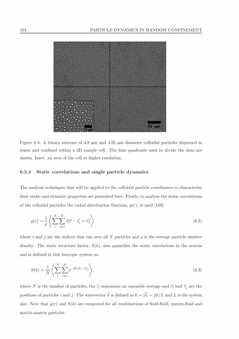
104 PARTICLE DYNAMICS IN RANDOM CONFINEMENT
Figure 6.4: A binary mixture of 3.9 µm and 4.95 µm diameter colloidal particles dispersed in
water and confined within a 2D sample cell. The four quadrants used to divide the data are
shown. Inset: an area of the cell at higher resolution.
6.3.4 Static correlations and single particle dynamics
The analysis techniques that will be applied to the colloidal particle coordinates to characterise
their static and dynamic properties are presented here. Firstly, to analyse the static correlations
of the colloidal particles the radial distribution function, g(r), is used [169]:
g(r) =1
ρ
⟨
N∑
i
N∑
j 6=i
δ[~r − ~rj + ~ri]
⟩
(6.2)
where i and j are the indices that run over all N particles and ρ is the average particle number
density. The static structure factor, S(k), also quantifies the static correlations in the system
and is defined in this isotropic system as:
S(k) =1
N
⟨
N∑
i
N∑
j 6=i
e−i~k·(~ri−~rj)
⟩
. (6.3)
where N is the number of particles, the 〈〉 represents an ensemble average and ~ri and ~rj are the
positions of particles i and j. The wavevector ~k is defined as k = |~k| = 2π/L and L is the system
size. Note that g(r) and S(k) are computed for all combinations of fluid-fluid, matrix-fluid and
matrix-matrix particles.
6.3 EXPERIMENTAL METHODS AND DATA ANALYSIS 105
The single particle dynamics are characterised by calculating the self part of the van
Hove correlation function [169], Gs(x, t). This corresponds to the probability distribution that
a particle has traveled a distance x in a time interval t:
Gs(x, t) =1
N
⟨
N∑
i=1
δ (x+ xi(0)− xi(t))
⟩
. (6.4)
Consequently, the particle mobility is measured in terms of the mean-squared displacement
(MSD),⟨
x2⟩
, which is defined as the second moment of Gs(x, t) [169]:
⟨
x2(t)⟩
=1
N
N∑
i=1
[xi(t)− xi(0)]2 =
N∑
i=1
x2(t)Gs(x, t) (6.5)
The non-Gaussian behaviour of the self part of the correlation function can be quantified by the
non-Gaussian parameter, α2, defined as:
α2(t) =
⟨
x4(t)⟩
3 〈x2(t)〉2− 1, (6.6)
where⟨
x4⟩
is the fourth moment of Gs(x, t). The level of any heterogeneity in the particle
dynamics can therefore be deduced from the time development of α2, which is zero for a Gaus-
sian distribution, and α2 > 0 for non-Gaussian behaviour. Together, the van Hove correlation
function and the non-Gaussian parameter are useful tools for characterising the degree of hetero-
geneity in particle motion across the sample. The logarithmic derivative is used to aid analysis
of the mean square displacement and is defined as:
z(t) =d[log
⟨
r2(t)⟩
]
d[log(t)](6.7)
where⟨
r2(t)⟩
=⟨
x2(t)⟩
+⟨
y2(t)⟩
and z represents the exponent of the mean square displacement
where⟨
r2(t)⟩
∝ tz [245]. The self-part of the intermediate scattering function (ISF) is defined
as:
Fs(k, t) =1
N
⟨
N∑
j=1
ei~k·[~rj(t)−~rj (0)]
⟩
. (6.8)
The ISF is probed at wavevectors corresponding to the first peak in the fluid-fluid S(k) averaged
over all the state points (k = 1.4 µm−1).
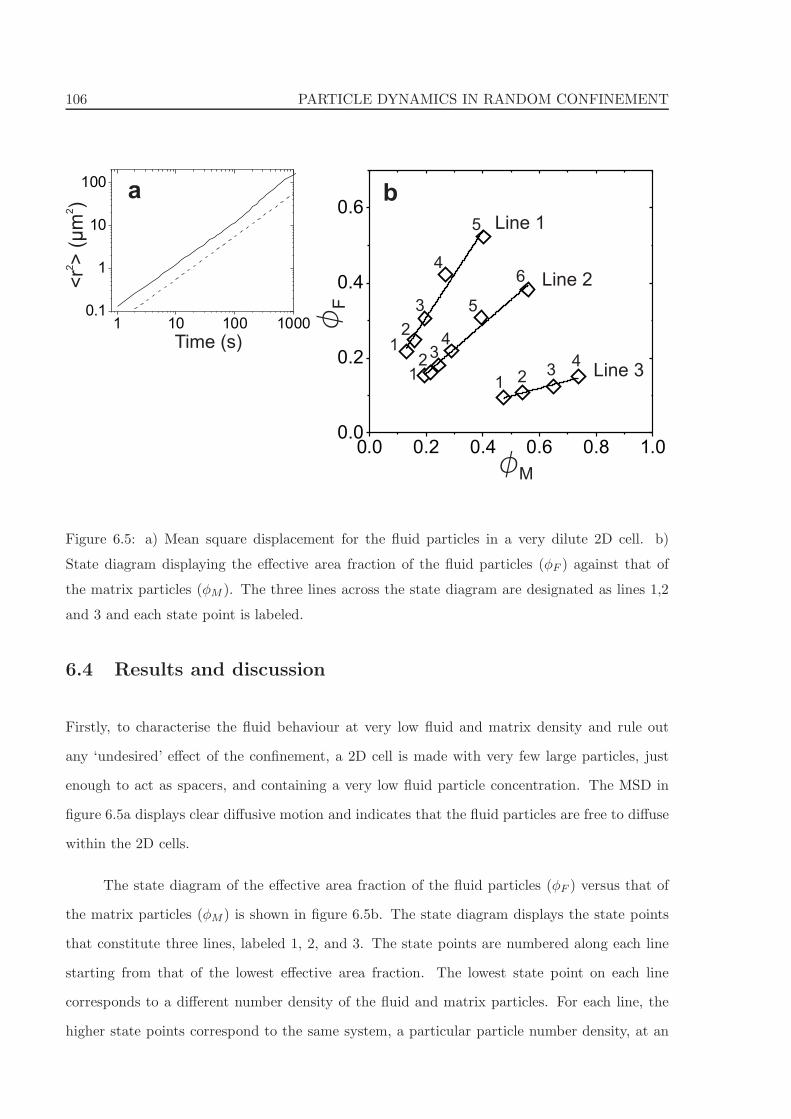
106 PARTICLE DYNAMICS IN RANDOM CONFINEMENT
0.0 0.2 0.4 0.6 0.8 1.00.0
0.2
0.4
0.6
1 10 100 10000.1
1
10
100
fM
fF
Line 1
Line 2
Line 3
1
5
1
6
1
4
2
3
4
234
5
2 3
<r
> (
m)
22
μ
Time ( )s
a b
Figure 6.5: a) Mean square displacement for the fluid particles in a very dilute 2D cell. b)
State diagram displaying the effective area fraction of the fluid particles (φF ) against that of
the matrix particles (φM ). The three lines across the state diagram are designated as lines 1,2
and 3 and each state point is labeled.
6.4 Results and discussion
Firstly, to characterise the fluid behaviour at very low fluid and matrix density and rule out
any ‘undesired’ effect of the confinement, a 2D cell is made with very few large particles, just
enough to act as spacers, and containing a very low fluid particle concentration. The MSD in
figure 6.5a displays clear diffusive motion and indicates that the fluid particles are free to diffuse
within the 2D cells.
The state diagram of the effective area fraction of the fluid particles (φF ) versus that of
the matrix particles (φM ) is shown in figure 6.5b. The state diagram displays the state points
that constitute three lines, labeled 1, 2, and 3. The state points are numbered along each line
starting from that of the lowest effective area fraction. The lowest state point on each line
corresponds to a different number density of the fluid and matrix particles. For each line, the
higher state points correspond to the same system, a particular particle number density, at an
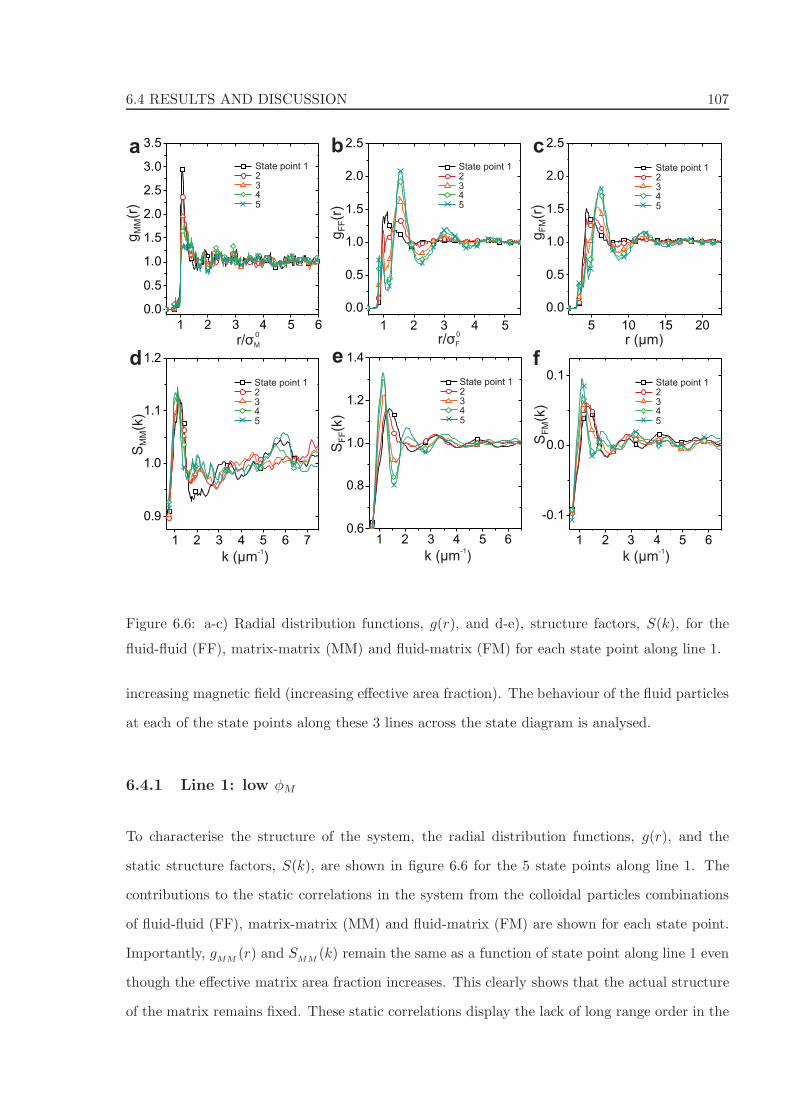
6.4 RESULTS AND DISCUSSION 107
1 2 3 4 5 6 7
0.9
1.0
1.1
1.2
1 2 3 4 5 6
0.0
0.5
1.0
1.5
2.0
2.5
3.0
3.5g
(r)
MM
r/σM
0
aState point 12345
1 2 3 4 5
0.0
0.5
1.0
1.5
2.0
2.5
State point 12345
g(r
)F
Fr/σF
0
b
1 2 3 4 5 60.6
0.8
1.0
1.2
1.4e
S(k
)F
F
k ( m )μ-1
State point 12345
d
S(k
)M
M
k ( m )μ-1
State point 12345
1 2 3 4 5 6
-0.1
0.0
0.1
5 10 15 20
0.0
0.5
1.0
1.5
2.0
2.5
State point 12345
g(r
)F
M
r ( m)μ
c
f
S(k
)F
M
k ( m )μ-1
State point 12345
Figure 6.6: a-c) Radial distribution functions, g(r), and d-e), structure factors, S(k), for the
fluid-fluid (FF), matrix-matrix (MM) and fluid-matrix (FM) for each state point along line 1.
increasing magnetic field (increasing effective area fraction). The behaviour of the fluid particles
at each of the state points along these 3 lines across the state diagram is analysed.
6.4.1 Line 1: low φM
To characterise the structure of the system, the radial distribution functions, g(r), and the
static structure factors, S(k), are shown in figure 6.6 for the 5 state points along line 1. The
contributions to the static correlations in the system from the colloidal particles combinations
of fluid-fluid (FF), matrix-matrix (MM) and fluid-matrix (FM) are shown for each state point.
Importantly, gMM
(r) and SMM
(k) remain the same as a function of state point along line 1 even
though the effective matrix area fraction increases. This clearly shows that the actual structure
of the matrix remains fixed. These static correlations display the lack of long range order in the
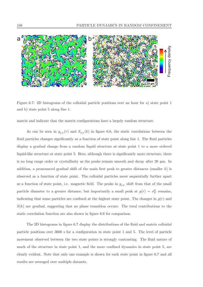
108 PARTICLE DYNAMICS IN RANDOM CONFINEMENT
a b
Fre
qu
en
cy d
en
sity
Figure 6.7: 2D histograms of the colloidal particle positions over an hour for a) state point 1
and b) state point 5 along line 1.
matrix and indicate that the matrix configurations have a largely random structure.
As can be seen in gFF
(r) and SFF
(k) in figure 6.6, the static correlations between the
fluid particles changes significantly as a function of state point along line 1. The fluid particles
display a gradual change from a random liquid structure at state point 1 to a more ordered
liquid-like structure at state point 5. Here, although there is significantly more structure, there
is no long range order or crystallinity as the peaks remain smooth and decay after 20 µm. In
addition, a pronounced gradual shift of the main first peak to greater distances (smaller k) is
observed as a function of state point. The colloidal particles move sequentially further apart
as a function of state point, i.e. magnetic field. The peaks in gFF
shift from that of the small
particle diameter to a greater distance, but importantly a small peak at g(r) = σ0F remains,
indicating that some particles are confined at the highest state point. The changes in g(r) and
S(k) are gradual, suggesting that no phase transition occurs. The total contributions to the
static correlation function are also shown in figure 6.6 for comparison.
The 2D histograms in figure 6.7 display the distributions of the fluid and matrix colloidal
particle positions over 3600 s for a configuration in state point 1 and 5. The level of particle
movement observed between the two state points is strongly contrasting. The fluid nature of
much of the structure in state point 1, and the more confined dynamics in state point 5, are
clearly evident. Note that only one example is shown for each state point in figure 6.7 and all
results are averaged over multiple datasets.
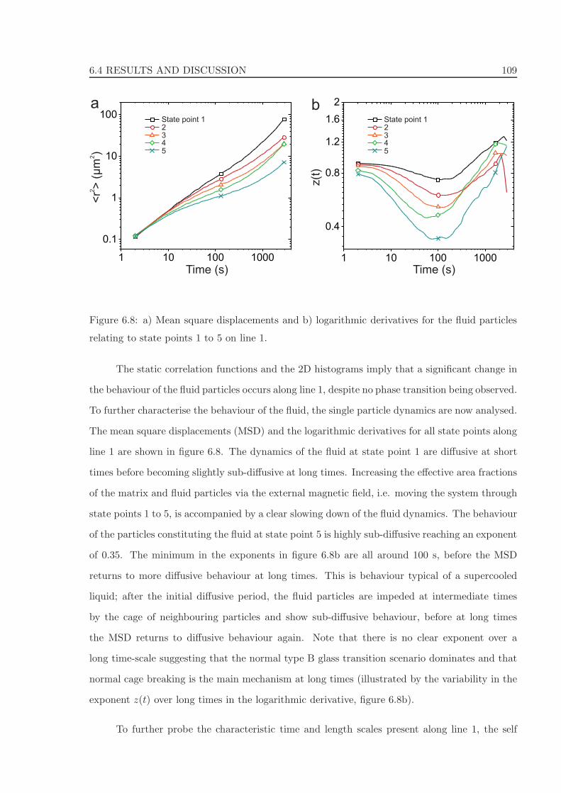
6.4 RESULTS AND DISCUSSION 109
1 10 100 1000
0.1
1
10
100
1 10 100 1000
0.4
0.8
1.2
1.6
2
Time (s) Time (s)
<r
> (
m)
22
μ
z(t
)
a bState point 12345
Figure 6.8: a) Mean square displacements and b) logarithmic derivatives for the fluid particles
relating to state points 1 to 5 on line 1.
The static correlation functions and the 2D histograms imply that a significant change in
the behaviour of the fluid particles occurs along line 1, despite no phase transition being observed.
To further characterise the behaviour of the fluid, the single particle dynamics are now analysed.
The mean square displacements (MSD) and the logarithmic derivatives for all state points along
line 1 are shown in figure 6.8. The dynamics of the fluid at state point 1 are diffusive at short
times before becoming slightly sub-diffusive at long times. Increasing the effective area fractions
of the matrix and fluid particles via the external magnetic field, i.e. moving the system through
state points 1 to 5, is accompanied by a clear slowing down of the fluid dynamics. The behaviour
of the particles constituting the fluid at state point 5 is highly sub-diffusive reaching an exponent
of 0.35. The minimum in the exponents in figure 6.8b are all around 100 s, before the MSD
returns to more diffusive behaviour at long times. This is behaviour typical of a supercooled
liquid; after the initial diffusive period, the fluid particles are impeded at intermediate times
by the cage of neighbouring particles and show sub-diffusive behaviour, before at long times
the MSD returns to diffusive behaviour again. Note that there is no clear exponent over a
long time-scale suggesting that the normal type B glass transition scenario dominates and that
normal cage breaking is the main mechanism at long times (illustrated by the variability in the
exponent z(t) over long times in the logarithmic derivative, figure 6.8b).
To further probe the characteristic time and length scales present along line 1, the self
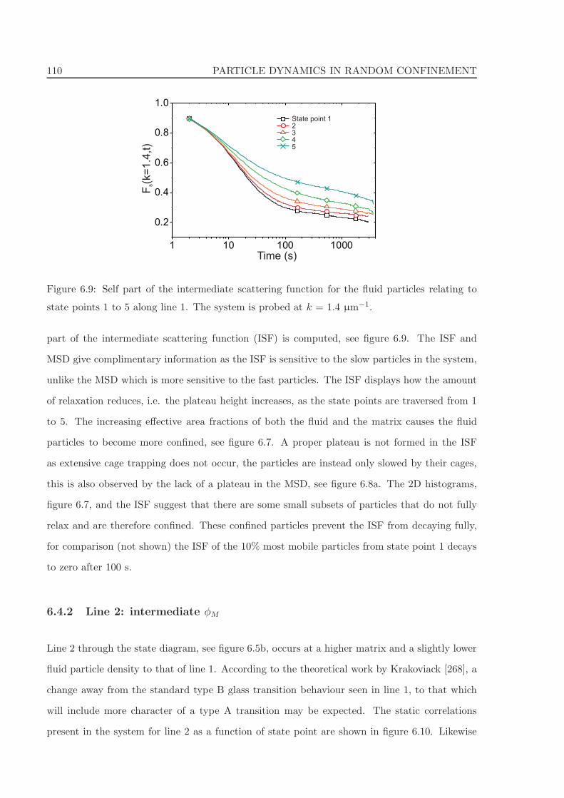
110 PARTICLE DYNAMICS IN RANDOM CONFINEMENT
1 10 100 1000
0.2
0.4
0.6
0.8
1.0
Time (s)
F(k
=1.4
,t)
s
State point 12345
Figure 6.9: Self part of the intermediate scattering function for the fluid particles relating to
state points 1 to 5 along line 1. The system is probed at k = 1.4 µm−1.
part of the intermediate scattering function (ISF) is computed, see figure 6.9. The ISF and
MSD give complimentary information as the ISF is sensitive to the slow particles in the system,
unlike the MSD which is more sensitive to the fast particles. The ISF displays how the amount
of relaxation reduces, i.e. the plateau height increases, as the state points are traversed from 1
to 5. The increasing effective area fractions of both the fluid and the matrix causes the fluid
particles to become more confined, see figure 6.7. A proper plateau is not formed in the ISF
as extensive cage trapping does not occur, the particles are instead only slowed by their cages,
this is also observed by the lack of a plateau in the MSD, see figure 6.8a. The 2D histograms,
figure 6.7, and the ISF suggest that there are some small subsets of particles that do not fully
relax and are therefore confined. These confined particles prevent the ISF from decaying fully,
for comparison (not shown) the ISF of the 10% most mobile particles from state point 1 decays
to zero after 100 s.
6.4.2 Line 2: intermediate φM
Line 2 through the state diagram, see figure 6.5b, occurs at a higher matrix and a slightly lower
fluid particle density to that of line 1. According to the theoretical work by Krakoviack [268], a
change away from the standard type B glass transition behaviour seen in line 1, to that which
will include more character of a type A transition may be expected. The static correlations
present in the system for line 2 as a function of state point are shown in figure 6.10. Likewise
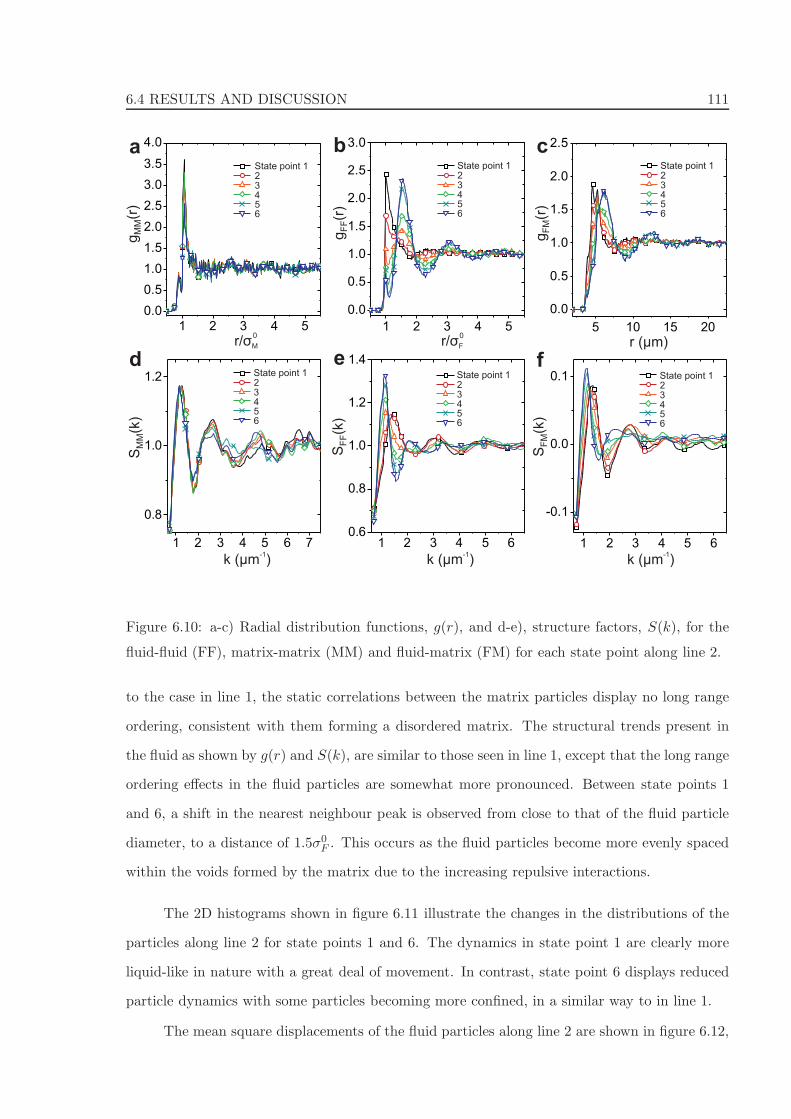
6.4 RESULTS AND DISCUSSION 111
1 2 3 4 5
0.0
0.5
1.0
1.5
2.0
2.5
3.0
3.5
4.0g
(r)
MM
r/σM
0
aState point 1234
65
1 2 3 4 5
0.0
0.5
1.0
1.5
2.0
2.5
3.0
g(r
)F
Fr/σF
0
bState point 1234
65
1 2 3 4 5 6 7
0.8
1.0
1.2d
S(k
)M
M
k ( m )μ-1
State point 1234
65
1 2 3 4 5 60.6
0.8
1.0
1.2
1.4e
S(k
)F
F
k ( m )μ-1
State point 1234
65
1 2 3 4 5 6
-0.1
0.0
0.1
5 10 15 20
0.0
0.5
1.0
1.5
2.0
2.5
g(r
)F
M
r ( m)μ
cState point 1234
65
f
S(k
)F
M
k ( m )μ-1
State point 1234
65
Figure 6.10: a-c) Radial distribution functions, g(r), and d-e), structure factors, S(k), for the
fluid-fluid (FF), matrix-matrix (MM) and fluid-matrix (FM) for each state point along line 2.
to the case in line 1, the static correlations between the matrix particles display no long range
ordering, consistent with them forming a disordered matrix. The structural trends present in
the fluid as shown by g(r) and S(k), are similar to those seen in line 1, except that the long range
ordering effects in the fluid particles are somewhat more pronounced. Between state points 1
and 6, a shift in the nearest neighbour peak is observed from close to that of the fluid particle
diameter, to a distance of 1.5σ0F . This occurs as the fluid particles become more evenly spaced
within the voids formed by the matrix due to the increasing repulsive interactions.
The 2D histograms shown in figure 6.11 illustrate the changes in the distributions of the
particles along line 2 for state points 1 and 6. The dynamics in state point 1 are clearly more
liquid-like in nature with a great deal of movement. In contrast, state point 6 displays reduced
particle dynamics with some particles becoming more confined, in a similar way to in line 1.
The mean square displacements of the fluid particles along line 2 are shown in figure 6.12,
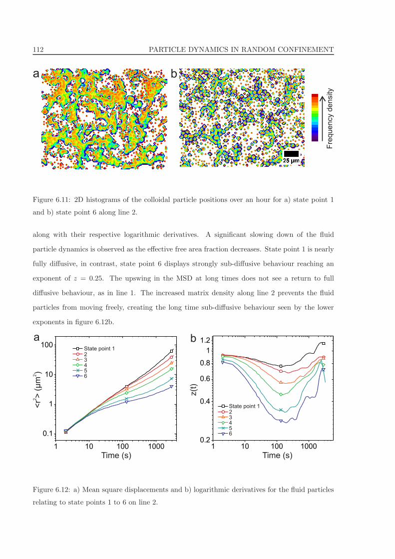
112 PARTICLE DYNAMICS IN RANDOM CONFINEMENT
a b
Fre
quency d
ensity
Figure 6.11: 2D histograms of the colloidal particle positions over an hour for a) state point 1
and b) state point 6 along line 2.
along with their respective logarithmic derivatives. A significant slowing down of the fluid
particle dynamics is observed as the effective free area fraction decreases. State point 1 is nearly
fully diffusive, in contrast, state point 6 displays strongly sub-diffusive behaviour reaching an
exponent of z = 0.25. The upswing in the MSD at long times does not see a return to full
diffusive behaviour, as in line 1. The increased matrix density along line 2 prevents the fluid
particles from moving freely, creating the long time sub-diffusive behaviour seen by the lower
exponents in figure 6.12b.
1 10 100 10000.2
0.4
0.6
0.8
1
1.2
1 10 100 1000
0.1
1
10
100
Time (s) Time (s)
<r
> (
m)
22
μ
z(t
)
a bState point 123456
State point 123456
Figure 6.12: a) Mean square displacements and b) logarithmic derivatives for the fluid particles
relating to state points 1 to 6 on line 2.
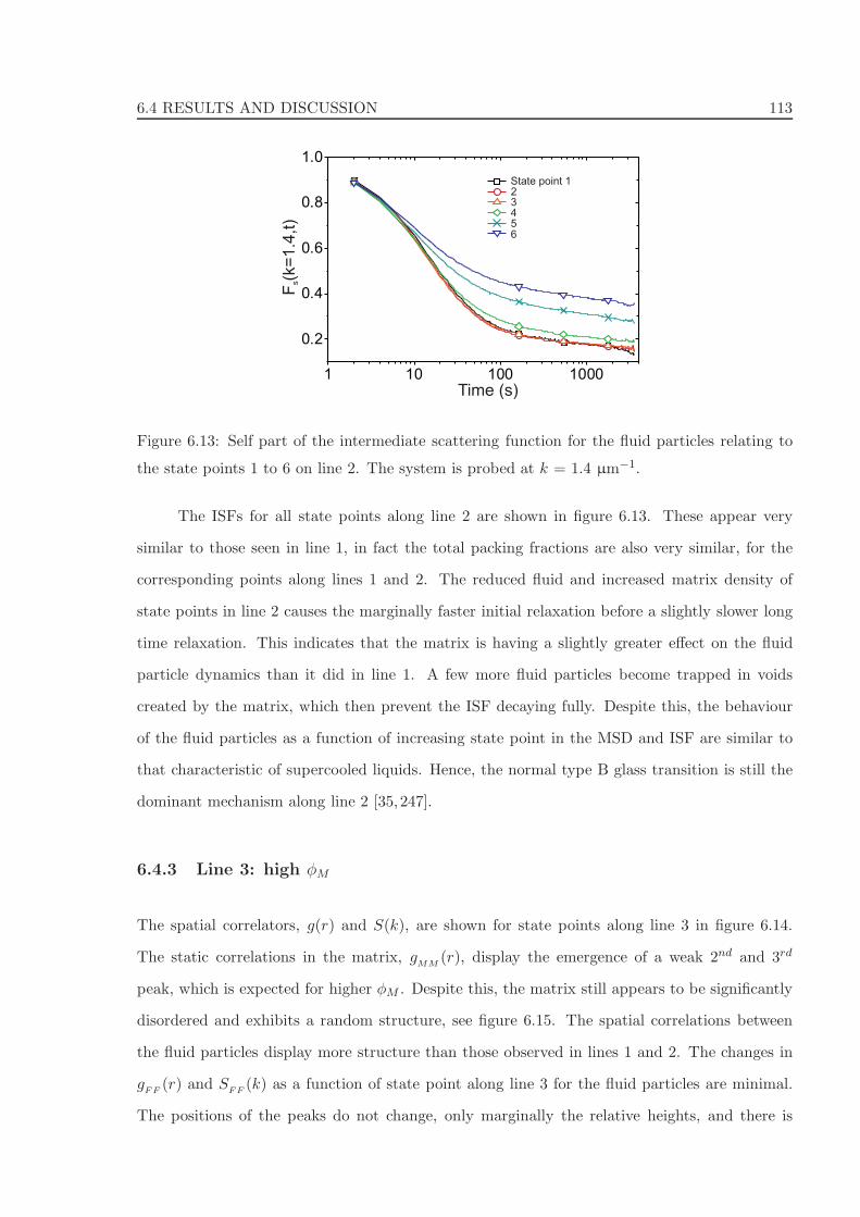
6.4 RESULTS AND DISCUSSION 113
1 10 100 1000
0.2
0.4
0.6
0.8
1.0
Time (s)
F(k
=1.4
,t)
s
State point 123456
Figure 6.13: Self part of the intermediate scattering function for the fluid particles relating to
the state points 1 to 6 on line 2. The system is probed at k = 1.4 µm−1.
The ISFs for all state points along line 2 are shown in figure 6.13. These appear very
similar to those seen in line 1, in fact the total packing fractions are also very similar, for the
corresponding points along lines 1 and 2. The reduced fluid and increased matrix density of
state points in line 2 causes the marginally faster initial relaxation before a slightly slower long
time relaxation. This indicates that the matrix is having a slightly greater effect on the fluid
particle dynamics than it did in line 1. A few more fluid particles become trapped in voids
created by the matrix, which then prevent the ISF decaying fully. Despite this, the behaviour
of the fluid particles as a function of increasing state point in the MSD and ISF are similar to
that characteristic of supercooled liquids. Hence, the normal type B glass transition is still the
dominant mechanism along line 2 [35,247].
6.4.3 Line 3: high φM
The spatial correlators, g(r) and S(k), are shown for state points along line 3 in figure 6.14.
The static correlations in the matrix, gMM
(r), display the emergence of a weak 2nd and 3rd
peak, which is expected for higher φM . Despite this, the matrix still appears to be significantly
disordered and exhibits a random structure, see figure 6.15. The spatial correlations between
the fluid particles display more structure than those observed in lines 1 and 2. The changes in
gFF
(r) and SFF
(k) as a function of state point along line 3 for the fluid particles are minimal.
The positions of the peaks do not change, only marginally the relative heights, and there is
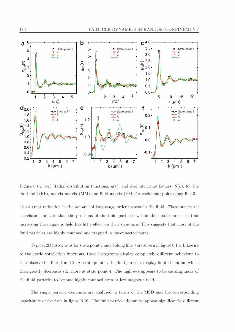
114 PARTICLE DYNAMICS IN RANDOM CONFINEMENT
5 10 15 20
0.0
0.5
1.0
1.5
2.0
2.5
3.0
3.5
4.0
1 2 3 4 5 6 70.2
0.4
0.6
0.8
1.0
1.2
1.4
1.6
1.8
2.0
1 2 3 4 5
0
1
2
3
4
5
6
g(r
)M
M
r/σM
0
aState point 1234
1 2 3 4 5
0
1
2
3
4
5
6
7
g(r
)F
F
r/σF
0
bState point 1234
d
S(k
)M
M
k ( m )μ-1
1 2 3 4 5 6 7
0.8
1.0
1.2
State point 1234
e
S(k
)F
F
k ( m )μ-1
1 2 3 4 5 6 7
-0.1
0.0
0.1
0.2
g(r
)F
M
r ( m)μ
cState point 1234
State point 1234
f
S(k
)F
M
k ( m )μ-1
State point 1234
Figure 6.14: a-c) Radial distribution functions, g(r), and d-e), structure factors, S(k), for the
fluid-fluid (FF), matrix-matrix (MM) and fluid-matrix (FM) for each state point along line 3.
also a great reduction in the amount of long range order present in the fluid. These structural
correlators indicate that the positions of the fluid particles within the matrix are such that
increasing the magnetic field has little effect on their structure. This suggests that most of the
fluid particles are highly confined and trapped in unconnected pores.
Typical 2D histograms for state point 1 and 4 along line 3 are shown in figure 6.15. Likewise
to the static correlation functions, these histograms display completely different behaviour to
that observed in lines 1 and 2. At state point 1, the fluid particles display limited motion, which
then greatly decreases still more at state point 4. The high φM appears to be causing many of
the fluid particles to become highly confined even at low magnetic field.
The single particle dynamics are analysed in terms of the MSD and the corresponding
logarithmic derivatives in figure 6.16. The fluid particle dynamics appear significantly different
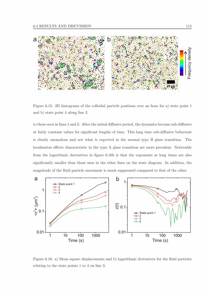
6.4 RESULTS AND DISCUSSION 115
Fre
quncy d
ensity
a b
Figure 6.15: 2D histograms of the colloidal particle positions over an hour for a) state point 1
and b) state point 4 along line 3.
to those seen in lines 1 and 2. After the initial diffusive period, the dynamics become sub-diffusive
at fairly constant values for significant lengths of time. This long time sub-diffusive behaviour
is clearly anomalous and not what is expected in the normal type B glass transition. The
localisation effects characteristic in the type A glass transition are more prevalent. Noticeable
from the logarithmic derivatives in figure 6.16b is that the exponents at long times are also
significantly smaller than those seen in the other lines on the state diagram. In addition, the
magnitude of the fluid particle movement is much suppressed compared to that of the other
1 10 100 10000.01
0.1
1
1 10 100 10000.01
0.1
1
Time (s) Time (s)
<r
> (
m)
22
μ
z(t
)
a bState point 1234
State point 1234
Figure 6.16: a) Mean square displacements and b) logarithmic derivatives for the fluid particles
relating to the state points 1 to 4 on line 3.
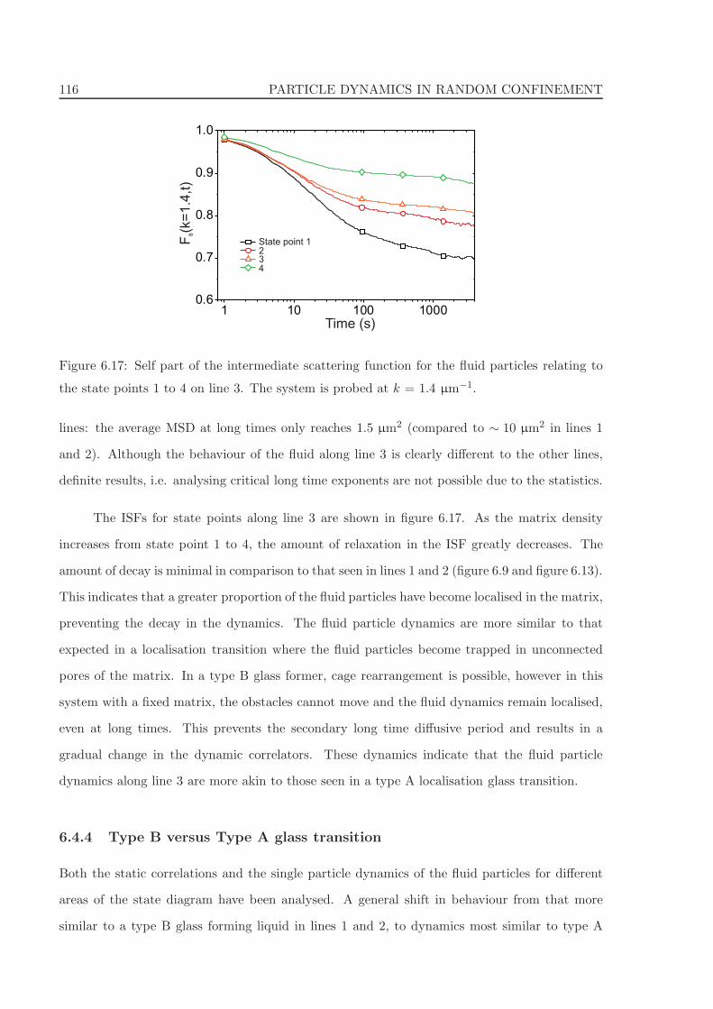
116 PARTICLE DYNAMICS IN RANDOM CONFINEMENT
1 10 100 10000.6
0.7
0.8
0.9
1.0
Time (s)
F(k
=1.4
,t)
s
State point 1234
Figure 6.17: Self part of the intermediate scattering function for the fluid particles relating to
the state points 1 to 4 on line 3. The system is probed at k = 1.4 µm−1.
lines: the average MSD at long times only reaches 1.5 µm2 (compared to ∼ 10 µm2 in lines 1
and 2). Although the behaviour of the fluid along line 3 is clearly different to the other lines,
definite results, i.e. analysing critical long time exponents are not possible due to the statistics.
The ISFs for state points along line 3 are shown in figure 6.17. As the matrix density
increases from state point 1 to 4, the amount of relaxation in the ISF greatly decreases. The
amount of decay is minimal in comparison to that seen in lines 1 and 2 (figure 6.9 and figure 6.13).
This indicates that a greater proportion of the fluid particles have become localised in the matrix,
preventing the decay in the dynamics. The fluid particle dynamics are more similar to that
expected in a localisation transition where the fluid particles become trapped in unconnected
pores of the matrix. In a type B glass former, cage rearrangement is possible, however in this
system with a fixed matrix, the obstacles cannot move and the fluid dynamics remain localised,
even at long times. This prevents the secondary long time diffusive period and results in a
gradual change in the dynamic correlators. These dynamics indicate that the fluid particle
dynamics along line 3 are more akin to those seen in a type A localisation glass transition.
6.4.4 Type B versus Type A glass transition
Both the static correlations and the single particle dynamics of the fluid particles for different
areas of the state diagram have been analysed. A general shift in behaviour from that more
similar to a type B glass forming liquid in lines 1 and 2, to dynamics most similar to type A

6.4 RESULTS AND DISCUSSION 117
1 10 100 1000
0
1
2
3
4
5
6
7
8
-20 -10 0 10 201E-7
1E-6
1E-5
1E-4
1E-3
0.01
0.1
1 Line 1 Point 1
Point 5Line 2 Point 1
Point 6Line 3 Point 1
Point 4
Line 1 Point 1
Line 2 Point 1
Line 3 Point 1
x ( m)μ Time ( )s
Px α
2
a bPoint 5
Point 6
Point 4
Figure 6.18: a) Self part of the van Hove correlation function at t = 1000 s in the x direction for
the first and last state point along each line. b) Non-Gaussian parameter, α2, in the x direction
as a function of time for the first and last state point along each line.
in line 3 are observed. The cuts through the state diagram are diagonal so all the behavioural
changes seen along the lines 1, 2 and 3 are likely to be a mixture to different extents of both
type B and A glass transitions. This is evidenced by the ISF not decaying to zero for any of the
lines, even in line 1 which is expected to represent the most type B-like behaviour. The ISF is
more sensitive to the slower particles than the MSD, which in lines 1 and 2 returned to diffusive
or nearly diffusive behaviour. This suggests that even at the lowest state points along each line
there are subsets of particles that are caged and have greatly different mobilities.
So far, the correlators analysed have been averaged over all the fluid particles. Now the
level of heterogeneity present in the fluid dynamics is investigated by computing the self part of
the van Hove correlation function and the non-Gaussian parameter, see figure 6.18. The trends
are shown for correlations in the x direction only, as the behaviour is not direction dependent.
The self part of the van Hove correlation function, Gs(x, t), is shown in figure 6.18a for
the first and last state points along each line, 1, 2 and 3, for time, t = 1000 s. The non-
Gaussian parameter (α2) is shown in figure 6.18b for the first and last state points along each
line as a function of time. Both Gs(x, t) and α2 indicate that the dynamics of the fluid particles
are generally quite heterogeneous. The trends in Gs(x, t) are as expected: the widths of the
distributions in Gs(x, t) are greater for the lowest state points (lower φM and φF ) than the
118 PARTICLE DYNAMICS IN RANDOM CONFINEMENT
highest state points along each line. This is consistent with the MSDs, which observed a slowing
down of the fluid dynamics as a function of state point along each line in the state diagram.
Comparing the level of dynamical heterogeneity between the lines, (α2 in figure 6.18)
shows that for line 3, the dynamics are significantly more non-Gaussian than for the other lines.
However, observation of the tails of the distributions in Gs(x, t) for line 3 shows that they are
reduced in width compared to lines 1 and 2, consistent with the MSD and the z(t) exponent
being a lot smaller. This increased non-Gaussian behaviour stems from the large subset of
particles which are very highly localised (∆x ≈ 0) and therefore contribute to the very steep
central peak in Gs(x, t) for line 3, which then increases α2, see figure 6.18.
Interestingly, the trends in α2 are not so clear cut. In lines 1 and 2, as φM and φF increase,
the fluid particle dynamics become increasingly heterogeneous. At low packing fractions along
these lines, few particles are caged and therefore most particles have similar behaviour. At
higher packing fractions, many of these particles become caged, the extent of which varies and
hence the dynamics become more heterogeneous. This increase in dynamical heterogeneity is
that expected as a fluid approaches a normal type B glass transition. In contrast, line 3 displays
the opposite trend. In line 3 the particle dynamics become more homogeneous at higher φM
and φF . At low packing fractions the system is very heterogeneous with most particles highly
localised, but with a small mobile subset. On increasing the packing fraction, this mobile subset
then becomes localised and the overall fluid particle dynamics become more homogeneous. This
behaviour suggests that the type A glass transition is the dominant mechanism along line 3 and
all the particle become highly localised in the matrix.
6.5 Conclusions
A 2D system has been created where large particles form a fixed random matrix around which
smaller particles, the ‘fluid’, are able to diffuse. All the colloidal particles in the system are super-
paramagnetic, hence, via increasing an external magnetic field, lines across a state diagram of
the effective area fraction of the matrix versus that of the fluid particles were scanned. The
behaviour of the fluid was mapped along three lines across the state diagram, lines 1, 2 and
3. In line 1, at low matrix density, the dynamic correlators of the MSD and self part of the
6.5 CONCLUSIONS 119
ISF indicated behavior similar to the early stages of a type B glass transition. The dynamics
of the fluid particles become increasingly non-Gaussian at large times as the total area fraction
increased. Line 2 started at a higher matrix and lower fluid density to line 1, and observed very
similar type B supercooled behaviour, but with a less pronounced upswing in the MSD. This
suggests that the fluid particles here are slightly more confined within the matrix and indicates
the weak presence of some dynamics characteristic of a type A localisation glass transition. Line
3 through the state diagram started at an even higher matrix and lower fluid area fraction. A
more gradual one step change in the dynamic correlators was observed, indicative of a type A
glass transition. The van Hove correlation function displayed that a large set of particles had
∆x ≈ 0, and therefore the majority of the particles were highly localised even at long times.
Qualitatively, good agreement is observed with both the mode coupling theory [34] and the
molecular dynamics simulations [35, 247] of a hard sphere fluid in a 3D hard sphere random
matrix. Thus also illustrating the similarities between 2D and 3D systems in terms of both the
nature of the transitions and the state diagram.
In order to further characterise the system, the aims are to: a) decompose the system
into dynamical subsets and characterise their mobility to get a better insight into the localised
particles. b) characterise the matrix further by computing the area fraction of the percolating
void and the average pore size.
Acknowledgments
This work is done in collaboration with Jurgen Horbach and Dirk Aarts.

120 PARTICLE DYNAMICS IN RANDOM CONFINEMENT
Summary
In this thesis, the behaviour of colloidal particles in two-dimensional (2D) systems is studied,
in particular grain boundaries and different types of confinement. The intrinsic softness and
the tunable interactions make colloidal systems ideal for manipulation with optical tweezers and
external magnetic fields whilst imaging with optical video microscopy.
In chapter 1, colloidal systems were introduced along with their basic characteristics,
including Brownian motion, their intrinsic softness and the fact that they can readily be observed
using standard optical microscopy, inherent to their timescales being on the order of seconds. In
chapter 2, the colloidal model system used in this thesis, the background behind the experimental
set-up and the experimental procedures were introduced. The construction of an optical tweezing
set-up in combination with an optical microscope was described which allowed manipulation and
simultaneous imaging of the single colloidal particles.
In chapter 3 a quasi-1D grain boundary in a 2D colloidal crystal was experimentally anal-
ysed. The fluctuations of the grain boundary were described by both spatial and dynamical
correlation functions of the interfacial profile. Real space expressions for these correlation func-
tions were derived from capillary wave theory. Good agreement was found for the values of the
key parameters that define the interface, the interface stiffness and mobility, from both the real
and Fourier space methodologies. In addition, a method of extracting the interfacial mobility
from analysis of the 1D random walk of the average interface position, as suggested by recent
simulations, was experientially verified providing good agreement with the other methods.
The grain boundary theme was continued in chapter 4, but this time rather than analysing
the interfacial fluctuations, the dynamics of the colloidal particles that make up the grain bound-
121
122 SUMMARY
ary were studied. It has long been hypothesised and also recently suggested in simulation, that
particles constituting grain boundaries can exhibit dynamics similar to supercooled liquids. The
mean square displacements of the grain boundary particles demonstrated a pronounced plateau
at intermediate times followed by a increase at longer times. Furthermore, the grain boundary
particle dynamics were found to be highly heterogeneous and chains of cooperatively moving
particles were observed. This observed dynamical behaviour, including consistent time evolution
of cluster sizes, diffusive particle dynamics and non-Gaussian distributions, is characteristic of
the particles in a supercooled liquid.
Chapter 5 addressed the effect of imposing 2D pentagonal confinement on the structure and
dynamics of spherical super-paramagnetic colloidal particles. An array of super-paramagnetic
colloidal particles were fixed in a pentagon shape by an optical tweezer. The state of the system
was characterised by Γ, which is a function of both the particle number density and the magnetic
field. In the first section, the behaviour of a 16 particle system, one that is commensurate to
the confining geometry was studied as the magnetic field was reduced. The particle dynamics
and orientational order displayed a gradual transition from a crystalline to confined liquid like
state at low interaction strength. In the second section, rather than varying the magnetic
field, the number of confined particles was increased from 10 to 21. Here, in contrast to the
first section, almost periodic trends in the orientational order of the system were observed.
These were coupled with an incoherent fluctuation in the dynamical behaviour of the confined
particles. The symmetry and orientational order in the packing arrangements greatly affected
the particle dynamics and the system was highly sensitive to the number of confined particles.
Re-entrant orientational ordering and fluctuating levels of dynamical behaviour were observed
as the confined number density increased.
In chapter 6 another form of 2D confinement was analysed: small colloidal particles, the
‘fluid’, were free to diffuse amongst a 2D fixed array of large particles, the ‘matrix’. All the
colloidal particles in the system were super-paramagnetic, hence, via increasing an external
magnetic field, in addition to varying the particle number densities, three lines across a state
diagram of the effective area fraction of the matrix versus that of the fluid particles were scanned.
In line 1 at low matrix density, the dynamic correlators of the fluid particles, including the
mean square displacement, displayed behaviour indicative of the early stages of a ‘normal’ glass

SUMMARY 123
transition. Across line 2 at intermediate matrix density, the dynamics of the fluid appeared to
be a mixture of that associated with both a ‘normal’ and a localisation glass transitions, though
still dominated by the ‘normal’ mechanism. In line 3 at high matrix density, the fluid particle
dynamics became highly localised, trapped within unconnected pores in the matrix. This lead to
indications of a localisation transition as expected at high matrix packing fractions. In all lines,
the dynamics were found to be very heterogeneous. These experimental results demonstrate
good agreement with both recent theory and simulations.

124
Bibliography
[1] D. Fennell Evans and H. Wennerstrom. The Colloidal domain where physics, chemistry,
biology and technology meet. Wiley-VCH, 2nd edition, 1999.
[2] C. A. Murray and D. G. Grier. Video microscopy of monodisperse colloidal systems. Annu.
Rev. Phys. Chem., 47:421–462, 1996.
[3] T. Graham. Liquid diffusion applied to analysis. Phil. Trans. Roy. Soc., 151:183–224,
1861.
[4] H. D. Goff. Colloidal aspects of ice cream - A review. Int. Dairy J., 7(6-7):363–373, 1997.
[5] T. F. Tadros. Colloids in paints, volume 6 of Colloids and interface science. Wiley-VCH,
2010.
[6] J. M. Martin and N. Ohmae. Colloidal Lubrication: General Principles, pages 1–13. John
Wiley and Sons, Ltd, 2008.
[7] A. G. Olabi and A. Grunwald. Design and application of magneto-rheological fluid. Mater.
and Des., 28(10):2658–2664, 2007.
[8] C. Graf and A. van Blaaderen. Metallodielectric colloidal core-shell particles for photonic
applications. Langmuir, 18(2):524–534, 2002.
[9] A. Einstein. Uber die von der molekularkinetischen theorie der warme geforderte bewegung
von in ruhenden flussigkeiten suspendierten teilchen. Ann. Phys., 17:549–560, 1905.
[10] M. D. Haw. Colloidal suspensions, brownian motion, molecular reality: a short history. J.
Phys.-Condes. Matter, 14(33):7769–7779, 2002.
[11] P. Habdas and E. R. Weeks. Video microscopy of colloidal suspensions and colloidal
crystals. Curr. Opin. Colloid Interface Sci., 7(3-4):196–203, 2002.
[12] P. Holmqvist, J. K. G. Dhont, and P. R. Lang. Anisotropy of Brownian motion caused
only by hydrodynamic interaction with a wall. Phys. Rev. E, 74(2):021402, 2006.
[13] N. J. Wagner and J. F. Brady. Shear thickening in colloidal dispersions. Phys. Today,
62(10):27–32, 2009.
125
126 BIBLIOGRAPHY
[14] W. C. K. Poon. Colloids as big atoms. Science, 304(5672):830–831, 2004.
[15] A. Yethiraj. Tunable colloids: control of colloidal phase transitions with tunable interac-
tions. Soft Matter, 3(9):1099–1115, 2007.
[16] P. N. Pusey and W. van Megen. Phase behaviour of concentrated suspensions of nearly
hard colloidal spheres. Nature, 320(6060):340–342, 1986.
[17] X. Ye, T. Narayanan, P. Tong, J. S. Huang, M. Y. Lin, B. L. Carvalho, and L. J. Fetters.
Depletion interactions in colloid-polymer mixtures. Phys. Rev. E, 54(6):6500–6510, 1996.
[18] U. Gasser, C. Eisenmann, G. Maret, and P. Keim. Melting of crystals in two dimensions.
Chem. Phys. Chem., 11(5):963–970, 2010.
[19] G. Fonnum, C. Johansson, A. Molteberg, S. Morup, and E. Aksnes. Characterisation of
Dynabeads by magnetization measurements and Mossbauer spectroscopy. J. Magn. Magn.
Mater., 293:41, 2005.
[20] V. Blickle, D. Babic, and C. Bechinger. Evanescent light scattering with magnetic colloids.
Appl. Phys. Lett., 87(10):101102, 2005.
[21] M. Ravnik, G. P. Alexander, J. M. Yeomans, and S. Zumer. Three-dimensional colloidal
crystals in liquid crystalline blue phases. Proc. Natl. Acad. Sci. USA, 108(13):5188–5192,
2011.
[22] J. R. Moffitt, Y. R. Chemla, S. B. Smith, and C. Bustamante. Recent advances in optical
tweezers, volume 77 of Annu. Rev. Biochem., pages 205–228. Annual Reviews, Palo Alto,
2008.
[23] L. J. Moore, R. D. Dear, M. D. Summers, R. P. A. Dullens, and G. A. D. Ritchie. Di-
rect observation of grain rotation-induced grain coalescence in two-dimensional colloidal
crystals. Nano Lett., 10(10):4266–4272, 2010.
[24] C. Jin-Ho, K. Soon-Jae, and P. Gyeong-Su. High-Tc superconductors in the two-
dimensional limit: [(Py−CnH2n+1)2HgI4]−Bi2Sr2Cam−1CumOy (m = 1 and 2). Science,
280(5369):1589–15921592, 1998.
[25] H. Gao, L. Zhang, W. D. Nix, C. V. Thompson, and E. Arzt. Crack-like grain-boundary
diffusion wedges in thin metal films. Acta Mater., 47(10):2865–2878, 1999.
[26] A. Shah, J. Meier, A. Buechel, U. Kroll, J. Steinhauser, F. Meillaud, H. Schade, and
D. Domine. Towards very low-cost mass production of thin-film silicon photovoltaic (PV)
solar modules on glass. Thin Solid Films, 502(1-2):292–299, 2006.
[27] T. Aste and D. Weaire. The persuit of perfect packing. IoP Publishing, 2000.
[28] U. Gasser. Crystallization in three- and two-dimensional colloidal suspensions. J. Phys.-
Condes. Matter, 21(20):203101, 2009.
BIBLIOGRAPHY 127
[29] D. G. A. L. Aarts, M. Schmidt, and H. N. W. Lekkerkerker. Direct visual observation of
thermal capillary waves. Science, 304(5672):847–850, 2004.
[30] J.J. Hoyt, Z.T. Trautt, and M. Upmanyu. Fluctuations in molecular dynamics simulations.
Math. Comput. Simul., 80:1382–1392, 2010.
[31] W. Rosenhain and D. Ewen. The intercrystalline cohesion of metals. J. Inst. Met., 10:119,
1913.
[32] H. Zhang, D. J. Srolovitz, J. F. Douglas, and J. A. Warren. Grain boundaries exhibit the
dynamics of glass-forming liquids. Proc. Natl. Acad. Sci. USA, 106(19):7735–7740, 2009.
[33] G. Laugel, J. Arichi, P. Bernhardt, M. Moliere, A. Kiennemann, F. Garin, and B. Louis.
Preparation and characterisation of metal oxides supported on SBA-15 as methane com-
bustion catalysts. C. R. Chimie, 12(67):731–739, 2009.
[34] V. Krakoviack. Liquid-glass transition of a fluid confined in a disordered porous matrix:
A Mode-Coupling theory. Phys. Rev. Lett., 94:065703, 2005.
[35] J. Kurzidim, D. Coslovich, and G. Kahl. Single-particle and collective slow dynamics of
colloids in porous confinement. Phys. Rev. Lett., 103(13):138303, 2009.
[36] T. Bauer, F. Hofling, T. Munk, E. Frey, and T. Franosch. The localization transition of
the two-dimensional Lorentz model. Eur. Phys. J.-Spec. Top., 189(1):103–118, 2010.
[37] P. W. Bridgman. Change of phase under pressure. i. The phase diagram of eleven sub-
stances with especial reference to the melting curve. Phys. Rev., 3(3):153–203, 1914.
[38] W. W. Wood and J. D. Jacobson. Preliminary results from a recalculation of the Monte
Carlo equation of state of hard spheres. J. Chem. Phys., 27(5):1207–1208, 1957.
[39] B. J. Alder and T. E. Wainwright. Phase transition for a hard sphere system. J. of Chem.
Phys., 27(5):1208–1209, 1957.
[40] W. G. Hoover and F. H. Ree. Melting transition and communal entropy for hard spheres.
J. Chem. Phys., 49(8):3609–3617, 1968.
[41] X. Batlle and A. Labarta. Finite-size effects in fine particles: magnetic and transport
properties. J. Phys. D-Appl. Phys., 35(6):R15–R42, 2002.
[42] D. J. Griffiths. Introduction to Electrodynamics. Prentice-Hall, Upper Saddle River, 3rd
edition, 1999.
[43] W. Sutherland. Dynamical theory of diffusion for non-electrolytes and the molecular mass
of albumin. Phil. Mag., 9:781–785, 1905.
[44] D. Drung, C. Assmann, J. Beyer, A. Kirste, M. Peters, F. Ruede, and T. Schurig. Highly
sensitive and easy-to-use SQUID sensors. IEEE Trans. Appl. Supercond., 17(2):699–704,
2007.
128 BIBLIOGRAPHY
[45] H. C. King. The history of the telescope. Courier Dover, 2003.
[46] A. Ashkin. Acceleration and trapping of particles by radiation pressure. Phys. Rev. Lett.,
24(4):156–159, 1970.
[47] A. Ashkin and J. M. Dziedzic. Optical levitation by radiation pressure. Appl. Phys. Lett.,
19(8):283–285, 1971.
[48] A. Ashkin, J. M. Dziedzic, J. E. Bjorkholm, and S. Chu. Observation of a single-beam
gradient force optical trap for dielectric particles. Optics Lett., 11:288, 1986.
[49] A. Ashkin and J. M. Dziedzic. Optical trapping and manipulation of viruses and bacteria.
Science, 235:1517, 1987.
[50] K. Svoboda and S. M. Block. Biological applications of optical forces. Annu. Rev. Biophys.
Biomolec. Struct., 23:247–285, 1994.
[51] K. O. Greulich and G. Pilarczyk. Laser tweezers and optical microsurgery in cellular
and molecular biology. working principles and selected applications. Cell. Mol. Biol.,
44(5):701–710, 1998.
[52] H. Zhang and K. K. Liu. Optical tweezers for single cells. J. R. Soc. Interface, 5(24):671–
690, 2008.
[53] R. W. Applegate, J. Squier, T. Vestad, J. Oakey, and D. W. M. Marr. Optical trapping,
manipulation, and sorting of cells and colloids in microfluidic systems with diode laser
bars. Opt. Express, 12(19):4390–4398, 2004.
[54] R. Andrew. Use of optical tweezers for colloid science. J. Colloid Interface Sci., 262(1):55–
59, 2003.
[55] D. G. Grier. Optical tweezers in colloid and interface science. Curr. Opin. Colloid Interface
Sci., 2(3):264–270, 1997.
[56] G. Dominguez-Espinosa, A. Synytska, A. Drechsler, C. Gutsche, K. Kegler, P. Uhlmann,
M. Stamm, and F. Kremer. Optical tweezers to measure the interaction between
poly(acrylic acid) brushes. Polymer, 49(22):4802–4807, 2008.
[57] M. Harada, M. Ishii, and H. Nakamura. Optically induced melting of colloidal crystals
and their recrystallization. H. Colloids Surf., B, 56(1-2):220–223, 2007.
[58] D. G. Grier. A revolution in optical manipulation. Nature, 424(6950):810–816, 2003.
[59] Y. Harada and T. Asakura. Radiation forces on a dielectric sphere in the Rayleigh scat-
tering regime. Opt. Commun., 124:529, 1996.
[60] P. A. M. Neto and H. M. Nussenzveig. Theory of optical tweezers. Europhys. Lett.,
50(5):702–708, 2000.

BIBLIOGRAPHY 129
[61] A. Mazolli, P. A. M. Neto, and H. M. Nussenzveig. Theory of trapping forces in optical
tweezers. Proc. R. Soc. London Ser. A-Math. Phys. Eng. Sci., 459(2040):3021–3041, 2003.
[62] A. Ashkin. Forces of a single-beam gradient laser trap on a dielectric sphere in the ray
optics regime. Biophysical Journal, 61:569, 1992.
[63] K. Sasaki, M. Koshioka, H. Misawa, N. Kitamura, and H. Masuhara. Pattern-formation
and flow-control of fine particles by laser-scanning micromanipulation. Opt. Lett., 16:1463,
1991.
[64] C. Mio, T. Gong, A. Terray, and D. W. M. Marr. Design of a scanning laser optical trap
for multiparticle manipulation. Rev. Sci. Instrum., 71:2196, 2000.
[65] K. Visscher, S. P. Gross, and S. M. Block. Construction of multiple-beam optical traps
with nanometer-resolution position sensing. IEEE J. Sel. Top. Quant. 2, page 1066, 1996.
[66] D. L. J. Vossen, A. van der Horst, M. Dogterom, and A. van Blaaderen. Optical tweezers
and confocal microscopy for simultaneous three-dimensional manipulation and imaging in
concentrated colloidal dispersions. Rev. Sci. Instrum., 75(9):2960–2970, 2004.
[67] J.-M. Fournier, M. M. Burns, and J. A. Golovchenko. Writing diffractive structures by
optical trapping. Proc. SPIE, 2406:101, 1995.
[68] E. R. Dufresne and D. G. Grier. Optical tweezer arrays and optical substrates created
with diffractive optics. Rev. Sci. Instrum., 69(5):1974–1977, 1998.
[69] E. Martin-Badosa, M. Montes-Usategui, A. Carnicer, J. Andilla, E. Pleguezuelos, and
I. Juvells. Design strategies for optimizing holographic optical tweezers set-ups. J. Opt.
A-Pure Appl. Opt., 9(8):S267–S277, 2007.
[70] M. Dienerowitz, G. Gibson, R. Bowman, and M. Padgett. Holographic tweezers: a platform
for plasmonics. Proc. SPIE, 8097:80971R, 2011.
[71] C. M. Creely, G. Volpe, G. P. Singh, M. Soler, and D. V. Petrov. Raman imaging of
floating cells. Optics Express, 13(16):6105–6110, 2005.
[72] T. Haraszti, A. E. M. Clemen, and J. P. Spatz. Biomimetic F-actin cortex models. Chem.
Phys. Chem., 10(16):2777–2786, 2009.
[73] K. Dholakia and P. Reece. Optical micromanipulation takes hold. Nano Today, 1(1):18–27,
2006.
[74] J. C. Crocker and D. G. Grier. Methods of digital video microscopy for colloidal studies.
J. Colloid Interface Sci., 179(1):298–310, 1996.
[75] C. Herring. The physics of powder metallurgy. McGraw-Hill Book Co., New York, 1951.
[76] J. P. Hirth and J. Lothe. Theory of dislocations. Wiley, New York, 2nd edition, 1982.
[77] J. M. Howe. Interfaces in Materials. Wiley, New York, 1997.
130 BIBLIOGRAPHY
[78] S. Graser, P. J. Hirschfeld, T. Kopp, R. Gutser, B. M. Andersen, and J. Mannhart. How
grain boundaries limit supercurrents in high-temperature superconductors. Nat. Phys.,
6(8):609–614, 2010.
[79] A. Hashibon, P. Schravendijk, C. Elsasser, and P. Gumbsch. Atomistic study of structure
and stability of thin Ni films on Fe surfaces. Philos. Mag., 89(34-36):3413–3433, 2009.
[80] P. Y. Huang, C. S. Ruiz-Vargas, A. M. van der Zande, W. S. Whitney, M. P. Levendorf,
J. W. Kevek, S. Garg, J. S. Alden, C. J. Hustedt, Y. Zhu, J. Park, P. L. McEuen, and
D. A. Muller. Grains and grain boundaries in single-layer graphene atomic patchwork
quilts. Nature, 469(7330):389–392, 2011.
[81] S. Yip. Nanocrystals: The strongest size. Nature, 391:532 – 533, 1998.
[82] H. Van Swygenhoven. Grain boundaries and dislocations. Science, 296:66 – 67, 2002.
[83] T. Zykova-Timan, R. E. Rozas, J. Horbach, and K. Binder. Computer simulation studies
of finite-size broadening of solid-liquid interfaces: From hard spheres to nickel. J. Phys.-
Condes. Matter, 21(46), 2009.
[84] Y. Huang and F. J. Humphreys. Measurements of grain boundary mobility during recrys-
tallization of a single-phase aluminium alloy. Acta Mater., 47(7):2259–2268, 1999.
[85] D. L. Medlin, S. M. Foiles, and D. Cohen. A dislocation-based description of grain
boundary dissociation: Application to a 90◦ ¡110¿ tilt boundary in gold. Acta Mater.,
49(18):3689–3697, 2001.
[86] S.B. Lee. Correlation between grain boundary faceting-defaceting transition and change
of grain boundary properties with temperature. Mater. Lett., 57:3779–3783, 2003.
[87] K. L. Merkle, L. J. Thompson, and F. Phillipp. In-situ HREM studies of grain boundary
migration. Interface Sci., 12:277–292, 2004.
[88] M. I. Mendelev and D. J. Srolovitz. Impurity effects on grain boundary migration. Modell.
Simul. Mater. Sci. Eng., 10:R79–R109, 2002.
[89] J. J. Hoyt, M. Asta, and A. Karma. Atomistic and continuum modeling of dendritic
solidification. Mater. Sci. Eng. R, 41(6):121–163, 2003.
[90] Z.T. Trautt and M. Upmanyu. Direct two-dimensional calculations of grain boundary
stiffness. Scr. Mater., 52:11751179, 2005.
[91] S. M. Foiles and J.J. Hoyt. Computation of grain boundary stiffness and mobility from
boundary fluctuations. Acta Mater., 54(12):3351–3357, 2006.
[92] K. G. F. Janssens, D. Olmstead, E. A. Holm, S. M. Foiles, S. J. Plimpton, and P. M.
Derlet. Computing the mobility of grain boundaries. Nat. Mater., 5:124–127, 2006.
BIBLIOGRAPHY 131
[93] D. L. Olmsted, S. M. Foiles, and E. A. Holm. Grain boundary interface roughening
transition and its effect on grain boundary mobility for non-faceting boundaries. Scripta
Mater., 57(12):1161–1164, 2007.
[94] D. L. Olmsted, E. A. Holm, and S. M. Foiles. Survey of computed grain boundary proper-
ties in face-centered cubic metals-II: Grain boundary mobility. Acta Mater., 57(13):3704–
3713, 2009.
[95] J. Hernandez-Guzman and E. R. Weeks. The equilibrium intrinsic crystal-liquid interface
of colloids. Proc. Natl. Acad. Sci. USA, 106(36):15198–15202, 2009.
[96] A. R. Bausch, M. J. Bowick, A. Cacciuto, A. D. Dinsmore, M. F. Hsu, D. R. Nelson,
M. G. Nikolaides, A. Travesset, and D. A. Weitz. Grain boundary scars and spherical
crystallography. Science, 299:1716–1718, 2003.
[97] P. Lipowsky, M. J. Bowick, J. H. Meinke, D. R. Nelson, and A. R. Bausch. Direct visual-
ization of dislocation dynamics in grain-boundary scars. Nat. Mater., 4:407–411, 2005.
[98] A. M. Alsayed, M. F. Islam, J. Zhang, P. J. Collings, and A. G. Yodh. Premelting at
defects within bulk colloidal crystals. Science, 309:1207–1210, 2005.
[99] V. W. A. de Villeneuve, L. Derendorp, D. Verboekend, E. C. M. Vermolen, W. K. Kegel,
H. N. W. Lekkerkerker, and R. P. A. Dullens. Grain boundary pinning in doped hard
sphere crystals. Soft Matter, 5:2448–2452, 2009.
[100] Z. T. Trautt, M. Upmanyu, and A. Karma. Interface mobility from interface random walk.
Science, 314:632–635, 2006.
[101] A. P. Young. Melting and the vector coulomb gas in 2 dimensions. Phys. Rev. B, 19:1855–
1866, 1979.
[102] D. R. Nelson and B. I. Halperin. Dislocation-mediated melting in 2 dimensions. Phys.
Rev. B, 19:2457–2484, 1979.
[103] J. M. Kosterlitz and D. J Thouless. Ordering, metastability and phase-transitions in 2
dimensional systems. J. Phys. C, 6:1181–1203, 1973.
[104] E. O. Hall. The deformation and ageing of mild steel 3. Discussion of results. Proc. Phys.
Soc. B, 64(381):747–753, 1951.
[105] N. J. Petch. The cleavage strength of polycrystals. J. Iron Steel Inst., 174:25–28, 1953.
[106] N. Hansen. HallPetch relation and boundary strengthening. Scripta Mater., 51(8):801–806,
2004.
[107] H. Suzuki. On the grain boundary migration induced by temperature gradient. J. Phys.
Soc. Jpn., 6(6):522–523, 1951.
132 BIBLIOGRAPHY
[108] M. Winning, G. Gottstein, and L. S. Shvindlerman. Stress induced grain boundary motion.
Acta Mater., 49(2):211–219, 2001.
[109] L. A. B. Mora. 2D and 3D Grain Growth Modelling and Simulation. Cuvillier Verlag,
Gottingen, 2008.
[110] H. Zhang, D. J. Srolovitz, J. F. Douglas, and J. A. Warren. Characterization of atomic
motion governing grain boundary migration. Phys. Rev. B, 74(11):115404, 2006.
[111] H. Zhang, D. J. Srolovitz, J. F. Douglas, and J. A. Warren. Atomic motion during the
migration of general [001] tilt grain boundaries in Ni. Acta Mater., 55(13):4527–4533,
2007.
[112] I. Toda-Caraballo, P. D. Bristowe, and C. Capdevila. A molecular dynamics study of grain
boundary free energies, migration mechanisms and mobilities in a BCC Fe20Cr alloy. Acta
Mater., 60(3):1116–1128, 2012.
[113] M. Upmanyu, R. W. Smith, and D. J. Srolovitz. Atomistic simulation of curvature driven
grain boundary migration. Interface Sci., 6(1):41–58, 1998.
[114] G. Gottstein, U Czubayko, D. A. Molodov, L. S. Shvindlerman, and W. Wunderlich.
In-situ observations of grain boundary migration. Mater. Sci. Forum, 204-206:99, 1996.
[115] M. Upmanyu, D. J. Srolovitz, L. S. Shvindlerman, and G. Gottstein. Misorientation
dependence of intrinsic grain boundary mobility: Simulation and experiment. Acta Mater.,
47(14):3901–3914, 1999.
[116] K. K. Mon, S. Wansleben, D. P. Landau, and K. Binder. Anisotropic surface tension, step
free energy, and interfacial roughening in the three-dimensional Ising model. Phys. Rev.
Lett., 60(8):708–711, 1988.
[117] C. L. Di Prinzio, B. J. G. Kriegel, and O. B. Nasello. Anisotropic migration of 2-
dimensional grain-boundaries. Acta Metall. Mater., 43(6):2269–2273, 1995.
[118] U. Wolf, F. Ernst, T. Muschik, M. W. Finnis, and H. F. Fischmeister. The influence of
grain-boundary inclination on the structure and energy of Sigma=3 grain-boundaries in
copper. Phil. Mag. A, 66(6):991–1016, 1992.
[119] A. P. Sutton and R. W. Balluffi. Overview 61. on geometric criteria for low interfacial
energy. Acta Metallurgica, 35(9):2177–2201, 1987.
[120] A. E. Lobkovsky, A. Karma, M. I. Mendelev, M. Haataja, and D. J. Srolovitz. Grain
shape, grain boundary mobility and the Herring relation. Acta Mater., 52:285–292, 2004.
[121] N. Eustathopoulos. Energetics of solid/liquid interfaces of metals and alloys. Intl. Met.
Rev., 28:189, 1983.
[122] H. Mykura and H. Gleiter. Can gravitational torques be used to study grain boundary
energy anisotropy? Scr. Metall. Mater., 13(2):137–140, 1979.
BIBLIOGRAPHY 133
[123] M. Upmanyu. Grain boundary stiffness based on a dislocation model. Scripta Mater.,
56(6):553–556, 2007.
[124] G. Gottstein, D. A. Molodov, and L. S. Shvindlerman. Grain boundary migration in
metals: Recent developments. Interface Sci., 6(1):7–22, 1998.
[125] M. Asta, C. Beckermann, A. Karma, W. Kurz, R. Napolitano, M. Plapp, G. Purdy,
M. Rappaz, and R. Trivedi. Solidification microstructures and solid-state parallels: Recent
developments, future directions. Acta Mater., 57(4):941–971, 2009.
[126] C. Deng and C. A. Schuh. Atomistic simulation of slow grain boundary motion. Phys.
Rev. Lett., 106(4):045503, 2011.
[127] L. Mandelstam. Ann. Phys, 41:609, 1913.
[128] M. P. A. Fisher, D. S. Fisher, and J. D. Weeks. Agreement of capillary-wave theory with
exact results for the interface profile of the two-dimensional Ising model. Phys. Rev. Lett.,
48(5):368–368, 1982.
[129] D. Bedeaux and J. D. Weeks. Correlation functions in the capillary wave model of the
liquid-vapor interface. J. Chem. Phys., 82(2):972, 1985.
[130] K. Binder, M. Muller, F. Schmid, and A. Werner. Simulation of interfaces between coex-
isting phases in materials. J. Comput.-Aided Mater. Des., 4:137, 1997.
[131] A. Werner, F. Schmid, M. Muller, and K. Binder. Anomalous size-dependence of interfacial
profiles between coexisting phases of polymer mixtures in thin-film geometry: A Monte
Carlo simulation. J. Chem. Phys., 107(19):8175–8188, 1997.
[132] K. L. Merkle. High-resolution electron microscopy of grain boundaries. Interface Sci.,
2:311, 1995.
[133] M. Furtkamp, P. Lejcek, and S. Tsurekawa. Grain boundary migration in Fe-3wt%Si
alloys. Interface Sci., 6(1-2):59–66, 1998.
[134] T. O. E. Skinner, D. G. A. L. Aarts, and R. P. A. Dullens. Grain-boundary fluctuations
in two-dimensional colloidal crystals. Phys. Rev. Lett., 105(16):168301, 2010.
[135] W. T. Read and W. Shockley. Dislocation models of crystal grain boundaries. Phys. Rev.,
78(3):275–289, 1950.
[136] E. Zaccarelli, C. Valeriani, E. Sanz, W. C. K. Poon, M. E. Cates, and P. N. Pusey.
Crystallization of hard-sphere glasses. Phys. Rev. Lett., 103(13):135704, 2009.
[137] P. Keblinski, S. R. Phillpot, D. Wolf, and H. Gleiter. Thermodynamic criterion for the sta-
bility of amorphous intergranular films in covalent materials. Phys. Rev. Lett., 77(14):2965,
1996.
134 BIBLIOGRAPHY
[138] D. Wolf. High-temperature structure and properties of grain boundaries: Long-range vs.
short-range structural effects. Curr. Opin. Solid State Mater. Sci., 5(5):435–443, 2001.
[139] H. Zhang and D. J. Srolovitz. Simulation and analysis of the migration mechanism of
Sigma 5 tilt grain boundaries in an FCC metal. Acta Mater., 54(3):623–633, 2006.
[140] C. Donati, J. F. Douglas, W. Kob, S. J. Plimpton, P. H. Poole, and S. C. Glotzer. Stringlike
cooperative motion in a supercooled liquid. Phys. Rev. Lett., 80(11):2338–2341, 1998.
[141] E. R. Weeks, J. C. Crocker, A. C. Levitt, A. Schofield, and D. A. Weitz. Three-
dimensional direct imaging of structural relaxation near the colloidal glass transition.
Science, 287(5453):627–631, 2000.
[142] P. G. Debenedetti and F. H. Stillinger. Supercooled liquids and the glass transition.
Nature, 410(6825):259–267, 2001.
[143] W. K. Kegel and A. van Blaaderen. Direct observation of dynamical heterogeneities in
colloidal hard-sphere suspensions. Science, 287(5451):290–293, 2000.
[144] M. M. Hurley and P. Harrowell. Kinetic structure of a 2-dimensional liquid. Phys. Rev.
E, 52(2):1694–1698, 1995.
[145] T. O. E. Skinner, D. G. A. L. Aarts, and R. P. A. Dullens. Supercooled dynamics of grain
boundary particles in two-dimensional colloidal crystals. J. Chem. Phys., 135(12):124711,
2011.
[146] K. H. Nagamanasa, S. Gokhale, R. Ganapathy, and A. K. Sood. Confined glassy dynamics
at grain boundaries in colloidal crystals. Proc. Natl. Acad. Sci. U. S. A., 108(28):11323–
11326, 2011.
[147] J. Q. Broughton and G. H. Gilmer. Grain-boundary shearing as a test for interface melting.
Model. Simul. Mater. Sci. Eng., 6(1):87–97, 1998.
[148] E. A. Holm and S. M. Foiles. How grain growth stops: A mechanism for grain-growth
stagnation in pure materials. Science, 328(5982):1138–1141, 2010.
[149] G. Gottstein and L. S. Shvindlerman. Grain Boundary Migration in Metals. CRC, Boca
Raton, FL, USA, 2nd edition, 2010.
[150] B. Schroder. Thin-film technology based on hydrogenated amorphous-silicon. Mater. Sci.
Eng. A-Struct. Mater. Prop. Microstruct. Process., 139:319–333, 1991.
[151] M. M. Trexler and N. N. Thadhani. Mechanical properties of bulk metallic glasses. Prog.
Mater. Sci., 55(8):759–839, 2010.
[152] M. D. Ediger. Spatially heterogeneous dynamics in supercooled liquids. Annu. Rev. Phys.
Chem., 51:99–128, 2000.
BIBLIOGRAPHY 135
[153] C. A. Angell, K. L. Ngai, G. B. McKenna, P. F. McMillan, and S. W. Martin. Relaxation
in glassforming liquids and amorphous solids. J. Appl. Phys., 88(6):3113–3157, 2000.
[154] R. Richert. Dynamics of nanoconfined supercooled liquids. Annu. Rev. Phys. Chem.,
62:65–84, 2011.
[155] R. A. Riggleman, K. Yoshimoto, J. F. Douglas, and J. J. de Pablo. Influence of confinement
on the fragility of antiplasticized and pure polymer films. Phys. Rev. Lett., 97(4):045502,
2006.
[156] S. Karmakar, C. Dasguptaa, and S. Sastry. Growing length and time scales in glass-forming
liquids. Proc. Natl. Acad. Sci. USA, 106(10):3675–3679, 2009.
[157] C. R. Berardi, K. Barros, J. F. Douglas, and W. Losert. Direct observation of stringlike
collective motion in a two-dimensional driven granular fluid. Phys. Rev. E, 81(4):041301,
2010.
[158] F. Hargreaves and R. J. Hills. J. Inst. Met., 41:257, 1929.
[159] C. J. Tweed, B. Ralph, and N. Hansen. The pinning by particles of low and high angle
grain boundaries during grain growth. Acta Metall., 32(9):1407–1414, 1984.
[160] M. Winning and A. D. Rollett. Transition between low and high angle grain boundaries.
Acta Mater., 53(10):2901–2907, 2005.
[161] G. S. Rohrer. Grain boundary energy anisotropy: A review. J. Mater. Sci., 46(18):5881–
5895, 2011.
[162] D. Wolf. A Read-Shockley model for high-angle grain-boundaries. Scr. Metall.,
23(10):1713–1718, 1989.
[163] A. P. Sutton and V. Vitek. On the structure of tilt grain-boundaries in cubic metals .1.
Symmetrical tilt boundaries. Philos. Trans. R. Soc. Lond. Ser. A-Math. Phys. Eng. Sci.,
309(1506):1–68, 1983.
[164] D. Schwartz, V. Vitek, and A. P. Sutton. Atomic structure of (001) twist boundaries in
f.c.c. metals - Structural unit model. Philos. Mag. A-Phys. Condens. Matter Struct. Defect
Mech. Prop., 51(4):499–520, 1985.
[165] W. Krakow. Atomic-structure of a σ = 21 grain-boundary. J. Mater. Res., 5(11):2658–
2662, 1990.
[166] V. Pontikis. Grain boundary structure and phase transformations : A critical review of
computer simulation studies and comparison with experiments. J Physique Colloques,
49(C5):C5–327–C5–336, 1988.
[167] P. Keblinski, D. Wolf, S. R. Phillpot, and H. Gleiter. Self-diffusion in high-angle fcc
metal grain boundaries by molecular dynamics simulation. Philos. Mag. A-Phys. Condens.
Matter Struct. Defect Mech. Prop., 79(11):2735–2761, 1999.
136 BIBLIOGRAPHY
[168] B. Schonfelder, G. Gottstein, and L. S. Shvindlerman. Comparative study of grain-
boundary migration and grain-boundary self-diffusion of 001 twist-grain boundaries in
copper by atomistic simulations. Acta Mater., 53(6):1597–1609, 2005.
[169] J. P. Hansen and I. R. McDonald. Theory of simple liquids. Academic Press, London, 3rd
edition, 2006.
[170] M. F. Ashby. Boundary defects, and atomistic aspects of boundary sliding and diffusional
creep. Surf. Sci., 31:498–542, 1972.
[171] R. Simon, T. Palberg, and P. Leiderer. Structurally determined Brownian dynamics in
ordered colloidal suspensions: Self-diffusion in fluid, supercooled, and crystalline phases.
J. Chem. Phys., 99(4):3030–3036, 1993.
[172] P. N. Pusey, E. Zaccarelli, C. Valeriani, E. Sanz, W. C. K. Poon, and M. E. Cates. Hard
spheres: Crystallization and glass formation. Phil.Transactions A, 367(1909):4993–5011,
2009.
[173] L. S. Shvindlerman, G. Gottstein, V. A. Ivanov, D. A. Molodov, D. Kolesnikov, and
W. Lojkowski. Grain boundary excess free volume - direct thermodynamic measurement.
J. Mater. Sci., 41(23):7725–7729, 2006.
[174] N. Giovambattista, S. V. Buldyrev, F. W. Starr, and H. E. Stanley. Connection between
Adam-Gibbs theory and spatially heterogeneous dynamics. Phys. Rev. Lett., 90(8):085506,
2003.
[175] W. Gotze and L. Sjogren. Comments on the mode coupling theory for structural relaxation.
Chem. Phys., 212(1):47–59, 1996.
[176] Y. Gebremichael, T. B. Schroder, F. W. Starr, and S. C. Glotzer. Spatially correlated
dynamics in a simulated glass-forming polymer melt: Analysis of clustering phenomena.
Phys. Rev. E, 64(5 Pt 1):051503, 2001.
[177] V. Teboul, A. Monteil, L. C. Fai, A. Kerrache, and S. Maabou. An investigation of string-
like cooperative motion in a strong network glass-former. Eur. Phys. J. B, 40:49, 2004.
[178] Q. H. Wei, C. Bechinger, and P. Leiderer. Single-file diffusion of colloids in one-dimensional
channels. Science, 287:625, 2000.
[179] C. R. Nugent, K. V. Edmond, H. N. Patel, and E. R. Weeks. Colloidal glass transition
observed in confinement. Phys. Rev. Lett., 99:025702, 2007.
[180] A. L. Boskey. Biomineralization: Conflicts, challenges, and opportunities. J. Cell.
Biochem., 30-31:83–91, 1998.
[181] F. Bresme and L. G. Camara. Computer simulation studies of crystallization under con-
finement conditions. Chem. Geo., 230(34):197–206, 2006.
BIBLIOGRAPHY 137
[182] J. Schmitt, G. Decher, W. J. Dressick, S. L. Brandow, R. E. Geer, R. Shashidhar, and
J. M. Calvert. Metal nanoparticle/polymer superlattice films: Fabrication and control of
layer structure. Adv. Mater., 9(1):61–65, 1997.
[183] M. S. Arayne, N. Sultana, and S. Noor Us. Fabrication of solid nanoparticles for drug
delivery. Pak. J. Pharm. Sci., 20(3):251–259, 2007.
[184] S. T. Cui, P. T. Cummings, and H. D. Cochran. Molecular dynamics simulation of the
rheological and dynamical properties of a model alkane fluid under confinement. J. Chem.
Phys., 111(3):1273–1280, 1999.
[185] Y. X. Zhu and S. Granick. Superlubricity: A paradox about confined fluids resolved. Phys.
Rev. Lett., 93(9):096101, 2004.
[186] S. Yamada. Nanotribology of symmetric and asymmetric liquid lubricants. Symmetry,
2(1):320–345, 2010.
[187] P. S. Dittrich and A. Manz. Lab-on-a-chip: microfluidics in drug discovery. Nat. Rev.
Drug Discov., 5(3):210–218, 2006.
[188] K. M. Unruh, T. E. Huber, and C. A. Huber. Melting and freezing behavior of indium
metal in porous glasses. Phys. Rev. B, 48(12):9021–9027, 1993.
[189] M. Sliwinska-Bartkowiak, J. Gras, R. Sikorski, R. Radhakrishnan, L. Gelb, and K. E.
Gubbins. Phase transitions in pores: Experimental and simulation studies of melting and
freezing. Langmuir, 15(18):6060–6069, 1999.
[190] D. D. Awschalom and J. Warnock. Supercooled liquids and solids in porous-glass. Phys.
Rev. B, 35(13):6779–6785, 1987.
[191] S. Granick. Motions and relaxations of confined liquids. Science, 253(5026):1374–1379,
1991.
[192] M. Heuberger, M. Zach, and N. D. Spencer. Density fluctuations under confinement:
When is a fluid not a fluid? Science, 292(5518):905–908, 2001.
[193] R. Haghgooie and P. S. Doyle. Structure and dynamics of repulsive magnetorheological
colloids in two-dimensional channels. Phys. Rev. E, 72(1):011405, 2005.
[194] C. Alba-Simionesco, B. Coasne, G. Dosseh, G. Dudziak, K. E. Gubbins, R. Radhakrishnan,
and M. Sliwinska-Bartkowiak. Effects of confinement on freezing and melting. J. Phys.-
Condes. Matter, 18(6):R15–R68, 2006.
[195] A. M. Homola, H. V. Nguyen, and G. Hadziioannou. Influence of monomer architecture on
the shear properties of molecularly thin polymer melts. J. Chem. Phys., 94(3):2346–2351,
1991.
138 BIBLIOGRAPHY
[196] F. Wang and Y. Zhao. The unique properties of the solid-like confined liquid films: A large
scale molecular dynamics simulation approach. Acta Mech. Solida Sinica, 24(2):101–116,
2011.
[197] R. Bubeck, C. Bechinger, S. Neser, and P. Leiderer. Melting and reentrant freezing of two-
dimensional colloidal crystals in confined geometry. Phys. Rev. Lett., 82(16):3364–3367,
1999.
[198] S. M. Ilett, A. Orrock, W. C. K. Poon, and P. N. Pusey. Phase-behavior of a model
colloid-polymer mixture. Phys. Rev. E, 51(2):1344–1352, 1995.
[199] A. Yethiraj and A. van Blaaderen. A colloidal model system with an interaction tunable
from hard sphere to soft and dipolar. Nature, 421(6922):513–517, 2003.
[200] K. Binder, S. Sengupta, and P. Nielaba. The liquid-solid transition of hard discs: first-
order transition or Kosterlitz-Thouless-Halperin-Nelson-Young scenario? J. Phys. Cond.
Matt., 14(9):2323–2333, 2002.
[201] N. Gribova, A. Arnold, T. Schilling, and C. Holm. How close to two dimensions does
a Lennard-Jones system need to be to produce a hexatic phase? J. Chem. Phys.,
135(5):054514, 2011.
[202] E. P. Bernard and W. Krauth. Two-step melting in two dimensions: first-order liquid-
hexatic transition. Phys. Rev. Lett., 107(15):155704, 2011.
[203] E. Azema, F. Radjaı, R. Peyroux, and G. Saussine. Force transmission in a packing of
pentagonal particles. Phys. Rev. E, 76(1):011301, 2007.
[204] K. Zahn and G. Maret. Dynamic criteria for melting in two dimensions. Phys. Rev. Lett.,
85(17):3656–3659, 2000.
[205] R. Bubeck, S. Neser, C. Bechinger, and P. Leiderer. Structure and dynamics of two-
dimensional colloidal crystals in confined geometry. Trends in Colloid and Interface Sci-
ence XII, volume 110, pages 41–45. Springer Berlin / Heidelberg, 1998.
[206] M. Saint Jean, C. Even, and C. Guthmann. Macroscopic 2D Wigner islands. Euro-
phys.Lett., 55(1):45–51, 2001.
[207] K. Mangold, J. Birk, P. Leiderer, and C. Bechinger. Binary colloidal systems in two-
dimensional circular cavities: Structure and dynamics. Phys. Chem. Chem. Phys.,
6(7):1623–1626, 2004.
[208] I. Hargittai. Fivefold symmetry. World Scientific, Singapore, 1992.
[209] T. Bauert, L. Merz, D. Bandera, M. Parschau, J. S. Siegel, and K.-H. Ernst. Building 2D
crystals from 5-fold-symmetric molecules. J. Am. Chem. Soc., 131(10):3460–3461, 2009.
[210] R. Penrose. Pentaplexity a class of non-periodic tilings of the plane. Math. Intelligencer,
2(1):32–37, 1979.
BIBLIOGRAPHY 139
[211] R. Luck. Durer-Kepler-Penrose, the development of pentagon tilings. Mater. Sci. Eng.:
A, 294296:263–267, 2000.
[212] D. Shechtman, I. Blech, D. Gratias, and J. W. Cahn. Metallic phase with long-range
orientational order and no translational symmetry. Phys. Rev. Lett., 53(20):1951, 1984.
[213] D. Levine and P. J. Steinhardt. Quasicrystals - a new class of ordered structures. Phys.
Rev. Lett., 53(26):2477–2480, 1984.
[214] D. Clery. Once-ridiculed discovery redefined the term crystal. Science, 334(6053):165,
2011.
[215] J. Mikhael, M. Schmiedeberg, S. Rausch, J. Roth, H. Stark, and C. Bechinger. Proliferation
of anomalous symmetries in colloidal monolayers subjected to quasiperiodic light fields.
Proc. Natl. Acad. Sci. USA, 107(16):7214–7218, 2010.
[216] V. G. Gryaznov, J. Heydenreich, A. M. Kaprelov, S. A. Nepijko, A. E. Romanov, and
J. Urban. Pentagonal symmetry and disclinations in small particles. Cryst. Res. Technol.,
34(9):1091–1119, 1999.
[217] D. V. Talapin, E. V. Shevchenko, M. I. Bodnarchuk, X. Ye, J. Chen, and C. B. Mur-
ray. Quasicrystalline order in self-assembled binary nanoparticle superlattices. Nature,
461(7266):964–967, 2009.
[218] H. Chen, Y. Gao, H. Yu, H. Zhang, L. Liu, Y. Shi, H. Tian, S. Xie, and J. Li. Structural
properties of silver nanorods with fivefold symmetry. Micron, 35(6):469–474, 2004.
[219] Y. Gao, L. Song, P. Jiang, L. F. Liu, X. Q. Yan, Z. P. Zhou, D. F. Liu, J. X. Wang, H. J.
Yuan, Z. X. Zhang, X. W. Zhao, X. Y. Dou, W. Y. Zhou, G. Wang, S. S. Xie, H. Y. Chen,
and J. Q. Li. Silver nanowires with five-fold symmetric cross-section. J. Cryst. Growth,
276(34):606–612, 2005.
[220] Y. N. Xia, Y. J. Xiong, B. Lim, and S. E. Skrabalak. Shape-controlled synthesis of
metal nanocrystals: Simple chemistry meets complex physics? Angew. Chem.-Int. Edit.,
48(1):60–103, 2009.
[221] M. D. Ball and D. J. Lloyd. Particles apparently exhibiting five-fold symmetry in Al-Li-
Cu-Mg alloys. Scr. Metall., 19(9):1065–1068, 1985.
[222] A. V. Anikeenko, N. N. Medvedev, A. Bezrukov, and D. Stoyan. Observation of fivefold
symmetry structures in computer models of dense packing of hard spheres. J. Non-Cryst.
Solids, 353(32-40):3545–3549, 2007.
[223] J. Carrasco, A. Michaelides, M. Forster, S. Haq, R. Raval, and A. Hodgson. A one-
dimensional ice structure built from pentagons. Nat. Mater., 8(5):427–431, 2009.
[224] N. C. Karayiannis, R. Malshe, J. J. de Pablo, and M. Laso. Fivefold symmetry as an
inhibitor to hard-sphere crystallization. Phys. Rev. E, 83(6):061505, 2011.

140 BIBLIOGRAPHY
[225] D. T. Lee and B. J. Schachter. Two algorithms for constructing a Delaunay triangulation.
Int. J. Comput. Inf. Sci., 9(3):219–242, 1980.
[226] R. P. A. Dullens, D. G. A. L. Aarts, and W. K. Kegel. Colloidal crystal-fluid interfaces.
Philos. Mag. Lett., 87(11):893–898, 2007.
[227] F. A. Lindemann. Phys. Z., 11:609, 1910.
[228] X. H. Zheng and J. C. Earnshaw. On the Lindemann criterion in 2D. Europhys. Lett.,
41(6):635–640, 1998.
[229] V. M. Bedanov, G. V. Gadiyak, and Y. E. Lozovik. On a modified Lindemann-like criterion
for 2D melting. Phys. Lett. A, 109(6):289–291, 1985.
[230] D. R. Nelson. Defects and geometry in condensed matter physics. Cambridge University
Press, 2002.
[231] D. Frenkel and B Smit. Understanding Molecular Simulation. From Algorithms to Appli-
cations,. Academic Press, London, 2nd ed. edition, 2002.
[232] A. Vikarchuk, M. Dorogov, A. Volkov, and N. Gryzunova. Disclination defects in substrates
as the sites of whisker growth. Russian Metallurgy (Metally), 2011(4):290–295, 2011.
[233] W. L. Miller and A. Cacciuto. Two-dimensional packing of soft particles and the soft
generalized Thomson problem. Soft Matter, 7(16):7552–7559, 2011.
[234] J. P. Hoogenboom, A. Yethiraj, A. K. van Langen-Suurling, J. Romijn, and A. van
Blaaderen. Epitaxial crystal growth of charged colloids. Phys. Rev. Lett., 89(25):256104,
2002.
[235] C. T. Kresge, M. E. Leonowicz, W. J. Roth, J. C. Vartuli, and J. S. Beck. Ordered
mesoporous molecular-sieves synthesized by a liquid-crystal template mechanism. Nature,
359(6397):710–712, 1992.
[236] A. A. Lucas, I. Derycke, Ph Lambin, J. P. Vigneron, L. Leherte, M. Elanany, J. M. Andr,
A. V. Larin, and D. P. Vercauteren. Confinement in molecular sieves: The pioneering
physical concepts. J. Mol. Catal. A: Chem., 305(12):16–23, 2009.
[237] N. Matsuoka and J. Murton. Frost weathering: Recent advances and future directions.
Permafrost Periglacial Process., 19(2):195–210, 2008.
[238] C. Toninelli, G. Biroli, and D. S. Fisher. Jamming percolation and glass transitions in
lattice models. Phys. Rev. Lett., 96(3):035702, 2006.
[239] A. J. Liu and S. R. Nagel. The jamming transition and the marginally jammed solid.
Annu. Rev. Condens. Matter Phys., 1:347–369, 2010.
[240] G. B. McKenna. Confit iii. Summary and perspectives on dynamics in confinement. Eur.
Phys. J.-Spec. Top., 141:291–301, 2007.

BIBLIOGRAPHY 141
[241] M. Alcoutlabi and G. B. McKenna. Effects of confinement on material behaviour at the
nanometre size scale. J. Phys.-Condes. Matter, 17(15):R461–R524, 2005.
[242] M. C. Bellissent-funel, J. Lal, and L. Bosio. Structural study of water confined in porous-
glass by neutron-scattering. J. Chem. Phys., 98(5):4246–4252, 1993.
[243] J. R. Dorfman and H. van Beijeren. Dynamical systems theory and transport coefficients:
A survey with applications to Lorentz gases. Physica A, 240(12):12–42, 1997.
[244] V. Krakoviack. Mode-coupling theory predictions for the dynamical transitions of partly
pinned fluid systems. Phys. Rev. E, 84(5):050501, 2011.
[245] J. Kurzidim, D. Coslovich, and G. Kahl. Impact of random obstacles on the dynamics of
a dense colloidal fluid. Phys. Rev. E, 82(4):041505, 2010.
[246] J. Kurzidim, D. Coslovich, and G. Kahl. Dynamic arrest of colloids in porous environments:
disentangling crowding and confinement. J. Phys.-Condes. Matter, 23(23):234122, 2011.
[247] K. Kim, K. Miyazaki, and S. Saito. Slow dynamics in random media: Crossover from glass
to localization transition. Europhys. Lett., 88(3):36002, 2009.
[248] F. He, L. M. Wang, and R. Richert. Dynamics of supercooled liquids in the vicinity of
soft and hard interfaces. Phys. Rev. B, 71:144205, 2005.
[249] C. L. Jackson and G. B. McKenna. The glass-transition of organic liquids confined to
small pores. J. Non-Cryst. Solids, 131:221–224, 1991.
[250] D. Sappelt and J. Jackle. The cooperativity length in models for the glass-transition. J.
Phys. A-Math. Gen., 26(24):7325–7341, 1993.
[251] G. Barut, P. Pissis, R. Pelster, and G. Nimtz. Glass transition in liquids: Two versus
three-dimensional confinement. Phys. Rev. Lett., 80(16):3543–3546, 1998.
[252] G. Biroli, J. P. Bouchaud, A. Cavagna, T. S. Grigera, and P. Verrocchio. Thermodynamic
signature of growing amorphous order in glass-forming liquids. Nat. Phys., 4(10):771–775,
2008.
[253] P. Pissis, A. Kyritsis, G. Barut, R. Pelster, and G. Nimtz. Glass transition in 2- and
3-dimensionally confined liquids. J. Non-Cryst. Solids, 235:444–449, 1998.
[254] L. D. Gelb and K. E. Gubbins. Pore size distributions in porous glasses: A computer
simulation study. Langmuir, 15(2):305–308, 1999.
[255] G. B. McKenna. Size and confinement effects in glass forming liquids: Perspectives on
bulk and nano-scale behaviours. J. Phys. IV, 10(P7):53–57, 2000.
[256] G. B. McKenna. Status of our understanding of dynamics in confinement: Perspectives
from Confit 2003. Eur. Phys. J. E, 12(1):191–194, 2003.
142 BIBLIOGRAPHY
[257] F. Hofling, T. Franosch, and E. Frey. Localization transition of the three-dimensional
Lorentz model and continuum percolation. Phys. Rev. Lett., 96(16):165901, 2006.
[258] K. Kim, K. Miyazaki, and S. Saito. Molecular dynamics studies of slow dynamics in random
media: Type A-B and reentrant transitions. Eur. Phys. J.-Spec. Top., 189(1):135–139,
2010.
[259] W. Gotze and L. Sjogren. Relaxation processes in supercooled liquids. Rep. Prog. Phys.,
55(3):241–376, 1992.
[260] W. Kob. The mode-coupling theory of the glass transition. ACS Symp. Ser., 676:28, 1997.
[261] A. J. Moreno and J. Colmenero. Anomalous dynamic arrest in a mixture of large and
small particles. Phys. Rev. E, 74(2):021409, 2006.
[262] H. Konig, R. Hund, K. Zahn, and G. Maret. Experimental realization of a model glass
former in 2D. J. Eur. Phys. E, 18(3):287–293, 2005.
[263] R. Bruning, D. A. St-Onge, S. Patterson, and W. Kob. Glass transitions in one-, two-
, three-, and four-dimensional binary lennard-jones systems. J. Phys.-Condes. Matter,
21(3):035117, 2009.
[264] D. Hajnal, J. M. Brader, and R. Schilling. Effect of mixing and spatial dimension on the
glass transition. Phys. Rev. E, 80(2):021503, 2009.
[265] N. Osterman, D. Babic, I. Poberaj, J. Dobnikar, and P. Ziherl. Observation of condensed
phases of quasiplanar core-softened colloids. Phys. Rev. Lett., 99(24):248301, 2007.
[266] J. A. Barker and D. Henderson. Perturbation theory and equation of state for fluids .2. A
successful theory of liquids. J. Chem. Phys., 47(11):4714–4721, 1967.
[267] A. A. Louis and R. Roth. Generalized depletion potentials. J. Phys. Condens. Matter,
13(33):L777–L784, 2001.
[268] V. Krakoviack. Tagged-particle dynamics in a fluid adsorbed in a disordered porous solid:
Interplay between the diffusion-localization and liquid-glass transitions. Phys. Rev. E,
79(6):061501, 2009.
List of publications
To date the following publications based upon work in this thesis have been submitted or are in
preparation:
Thomas O. E. Skinner, Dirk G. A. L. Aarts and Roel P. A. Dullens, (2010), Grain-boundary
fluctuations in two-dimensional colloidal crystals, Phys. Rev. Lett. 105, 168301, Editors Sug-
gestion, http://link.aps.org/doi/10.1103/PhysRevLett.105.168301, (Chapter 3)
Thomas O. E. Skinner, Dirk G. A. L. Aarts and Roel P. A. Dullens, (2011), Supercooled dynamics
of grain-boundary particles in colloidal crystals, J. Chem. Phys. 135, 124711,
http://dx.doi.org/10.1063/1.3640417, (Chapter 4)
Thomas O. E. Skinner, Henry Martin, Dirk G. A. L. Aarts and Roel P. A. Dullens, (2012), Frus-
trated crystallisation and melting in two-dimensional pentagonal confinement, In preparation,
(Chapter 5)
Thomas O. E. Skinner, Jurgen Horbach and Roel P. A. Dullens, (2012), Dynamics of a colloidal
fluid confined in a 2D random matrix, In preparation, (Chapter 6)
143

144

Acknowledgments
I would like to thank Roel for all his help, ideas and enthusiasm over the last 3.5 years and to
Dirk for his additional input. I would like to thank Liz who showed me the ropes back at the
very beginning, to Harry and Oli for making the first 2 years never dull, to Mike and Sam for
making the latter two years highly enjoyable, to Alice, Paola and Julia for making the Dullens
office good fun and to Tara and my family for their support.
145


![Kinetics of diffusion induced grain boundary migration of [100] twist boundaries in the Cu(Zn) system](https://static.fdokumen.com/doc/165x107/631c6051a906b217b906ec8b/kinetics-of-diffusion-induced-grain-boundary-migration-of-100-twist-boundaries.jpg)