VAPOR PRESSURES OF NARROW FRACTIONS

DERIVED FROM AN INDUSTRIAL SHALE

GASOLINE FRACTION

Z. S. Baird1, M. Listak1*

1Tallinn University of Technology, School of Engineering, Department of Energy Technology, Ehitajate tee 5,

19086 Tallinn, Estonia

*E-mail: madis.listak@ttu.ee

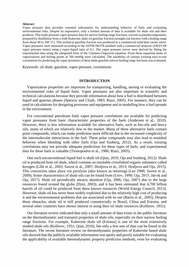
Abstract

Vapor pressure data provides essential information for understanding behavior of fuels and evaluating

environmental risks. Despite its importance, only a limited amount of data is available for shale oils and their

products. This study presents vapor pressure data for narrow boiling range fractions, viewed as pseudocomponents,

prepared by distillation from a wide Kukersite shale oil gasoline fraction (straight-run fraction with a boiling range

from about 40 to 200 °C). This technical gasoline fraction was produced in a commercial solid heat carrier retort.

Vapor pressures were measured according to the ASTM D6378 standard with a commercial analyzer (ERAVAP

vapor pressure tester) using a vapor-liquid ratio of 4:1. The vapor pressure curves were derived by fitting the

experimental data using the integrated form of the Clausius-Clapeyron equation. From these equations heats of

vaporizations and boiling points at 760 mmHg were calculated. The suitability of various existing easy-to-use

correlations for predicting the vapor pressures of these shale gasoline narrow boiling range fractions was evaluated.

Keywords: oil shale, gasoline, vapor pressure, correlations

INTRODUCTION

Vaporization properties are important for transporting, handling, storing or evaluating the

environmental risks of liquid fuels. Vapor pressures are also important in scientific and

technical calculations because they provide information about how a fuel is distributed between

liquid and gaseous phases (Spencer and Cliath, 1983; Riazi, 2005). For instance, they can be

used in calculations for designing processes and equipment and in modelling how a fuel spreads

in the environment.

For conventional petroleum fuels vapor pressure correlations are available for predicting

vapor pressures from basic characteristic properties of the fuels (Andersen et al., 2010).

However, there is less information available for alternative fuels, such as bio-oils and heavy

oils, many of which are relatively new to the market. Many of these alternative fuels contain

polar compounds, which can make prediction more difficult due to the increased complexity of

the intermolecular interactions in the fuel. These polar compounds may also lead to nonideal

behavior when blending with other fuels (Oja and Suuberg, 2012). As a result, existing

correlations may not provide adequate predictions for these types of fuels, and experimental

data for these fuels is valuable (Tsonopoulos et al., 1986; Riazi, 2005).

One such unconventional liquid fuel is shale oil (Qian, 2010; Oja and Suuberg, 2012). Shale

oil is produced from oil shale, which contains an insoluble crosslinked organic substance called

kerogen (Lille et al., 2003; Savest et al., 2007; Hruljova et al., 2013; Hruljova and Oja, 2015).

This conversion takes place via pyrolysis (also known as retorting) (Lee 1990; Savest et al.,

2009). Some characteristics of shale oils can be found from (Urov, 1999; Oja, 2015; Järvik and

Oja, 2017). Shale oil periodically attracts attention (Oja, 2006; Oja, 2007) due to the large

resources found around the globe (Dyni, 2003), and it has been estimated that 4,700 billion

barrels of oil could be produced from these known resources (World Energy Council, 2013).

However, shale oil has never been widely exploited due to the relatively high cost of producing

it and the environmental problems that are associated with its use (Bartis et al., 2005). Despite

these obstacles, shale oil is still produced commercially in Brazil, China and Estonia, and

several other countries have shown interest in using their oil shale resources (Kollerov, 1951).

Our literature review indicated that only a small amount of data exists in the public literature

on the thermodynamic and transport properties of shale oils, especially on their narrow boiling

range fractions. For example, Kukersite shale oil (Estonia) is one of the most extensively

studied shale oils (Kollerov, 1951; Qian, 2010), but only a few sets of data can be found in the

literature. The recent literature review on thermodynamic properties of Kukersite based shale

oils showed that the publicly available information was spotty and poorly suitable for evaluating

the applicability of available thermodynamic property prediction methods, even for evaluating

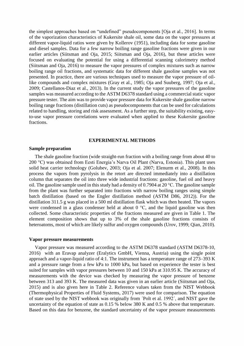
the simplest approaches based on “undefined” pseudocomponents [Oja et al., 2016]. In terms

of the vaporization characteristics of Kukersite shale oil, some data on the vapor pressures at

different vapor-liquid ratios were given by Kollerov (1951), including data for some gasoline

and diesel samples. Data for a few narrow boiling range gasoline fractions were given in our

earlier articles (Siitsman and Oja, 2015; Siitsman and Oja, 2016), but these articles were

focused on evaluating the potential for using a differential scanning calorimetry method

(Siitsman and Oja, 2016) to measure the vapor pressures of complex mixtures such as narrow

boiling range oil fractions, and systematic data for different shale gasoline samples was not

presented. In practice, there are various techniques used to measure the vapor pressure of oil-

like compounds and complex mixtures (Gray et al., 1985; Oja and Suuberg, 1997; Oja et al.,

2009; Castellanos-Diaz et al., 2013). In the current study the vapor pressures of the gasoline

samples was measured according to the ASTM D6378 standard using a commercial static vapor

pressure tester. The aim was to provide vapor pressure data for Kukersite shale gasoline narrow

boiling range fractions (distillation cuts) as pseudocomponents that can be used for calculations

related to handling, storing and risk assessment. As a further step, the suitability existing, easy-

to-use vapor pressure correlations were evaluated when applied to these Kukersite gasoline

fractions.

EXPERIMENTAL METHODS

Sample preparation

The shale gasoline fraction (wide straight-run fraction with a boiling range from about 40 to

200 °C) was obtained from Eesti Energia’s Narva Oil Plant (Narva, Estonia). This plant uses

solid heat carrier technology (Golubev, 2003; Oja et al. 2007; Elenurm et al., 2008). In this

process the vapors from pyrolysis in the retort are directed immediately into a distillation

column that separates the oil into three wide industrial fractions: gasoline, fuel oil and heavy

oil. The gasoline sample used in this study had a density of 0.7904 at 20 °C. The gasoline sample

from the plant was further separated into fractions with narrow boiling ranges using simple

batch distillation (based on the Engler distillation method (ASTM D86, 2012)). For the

distillation 311.5 g was placed in a 500 ml distillation flask which was then heated. The vapors

were condensed in a glass condenser held at about 0 °C, and the liquid gasoline was then

collected. Some characteristic properties of the fractions measured are given in Table 1. The

element composition shows that up to 3% of the shale gasoline fractions consists of

heteroatoms, most of which are likely sulfur and oxygen compounds (Urov, 1999; Qian, 2010).

Vapor pressure measurements

Vapor pressure was measured according to the ASTM D6378 standard (ASTM D6378-10,

2016) with an Eravap analyzer (Eralytics GmbH, Vienna, Austria) using the single point

approach and a vapor-liquid ratio of 4:1. The instrument has a temperature range of 273–393 K

and a pressure range from a few kPa to 1000 kPa, but based on experience the tester is best

suited for samples with vapor pressures between 10 and 150 kPa at 310.95 K. The accuracy of

measurements with the device was checked by measuring the vapor pressure of benzene

between 313 and 393 K. The measured data was given in an earlier article (Siitsman and Oja,

2015) and is also given here in Table 2. Reference values taken from the NIST Webbook

(Thermophysical Properties of Fluid Systems, 2017) were used for comparison. The equation

of state used by the NIST webbook was originally from ´Polt et al. 1992´, and NIST gave the

uncertainty of the equation of state as 0.15 % below 380 K and 0.5 % above that temperature.

Based on this data for benzene, the standard uncertainty of the vapor pressure measurements

presented here was estimated to be 0.66 kPa (expanded uncertainty of 1.5 kPa at the 95 % level).

This was estimated by calculating the standard deviation of the difference between the

measured and reference data points. However, the Eravap also had a maximum positive bias of

0.84 kPa (the bias increase with a boiling point of the sample), which was also shown in an

earlier article from our research group (Siitsman and Oja, 2015).

Measurement of other characteristic properties

Densities were measured using a DMA 5000M density meter (Anton Paar GmbH, Graz,

Austria). The instrument has reproducibility of 0.00005 g/cm³. For gasoline measurements

expanded uncertainties at the 95 % level were evaluated to be of 0.0003g cm-3.

Hydrogen and carbon contents were measured using an Exeter element analyzer (Exeter

Analytical Inc., North Chelmsford, MA, USA). Expanded uncertainties at the 95 % level were

evaluated to be of 0.17 wt% for hydrogen and 0.72 wt% for carbon.

RESULTS AND DISCUSSION

Vapor pressure data

The experimental vapor pressure data for the 8 shale gasoline fractions is given in Table 3

and is shown graphically in Figure 1. The vapor pressures for all the fractions exhibited a linear

trend on a lnP versus 1/T plot, and values for the R2 correlation coefficient were greater than

0.999 for all the samples except Fraction 6 (which had an R2 of 0.997). Therefore, the integrated

form of the Clausius-Clapeyron equation (Equation 1) was fit to the experimental data for each

fraction.

𝑙𝑛 𝑃 = −𝐴

𝑇+ 𝐵 =

−∆𝐻𝑣𝑎𝑝

𝑅𝑇+ 𝐵 (1)

In the Equation 1 P is the vapor pressure (kPa), ΔHvap is the heat of vaporization (J mol-1), T is

the temperature (K), B and A are fitting constants and R is the ideal gas constant (J mol-1 K-1).

The heat of vaporization and B are given in Table 4 for each of the fractions. The inflection

region around of the fractions 6 and 8, where the heat of vaporization (ΔHvap) and B values go

through slight “local minimum” at the fraction 7, can be attributed to occurrence of some

specific dominant structures in this boiling range. Normal boiling points (101.325 kPa) were

also calculated using Equation 1, and these are also reported in Table 4.

Evaluation of prediction methods when applied to shale gasoline

A number of equations and graphs, with various levels of complexity, have been developed

for predicting the vapor pressures of fuels, and here only those that are easy to use (i.e. based

on conveniently measureable input parameters) are evaluated. Correlations that require the

critical temperature, critical pressure and acentric factor are not considered here. Other methods

for estimating vapor pressures also exist, such as a correlation based on the distillation

temperatures of a sample and another based on the boiling points of narrow fractions of the

sample (Baird, 1981). These were not tested, however, because the required input data was not

available. The selected correlations were (1) a correlation from Van Kranen and Van Nes (Nes

and Westen, 1951), (2) the Maxwell and Bonnell correlation (Maxwell and Bonnell, 1955;

Maxwell and Bonnell, 1957) and (3) a modification to the Maxwell and Bonnell correlation

presented by Tsonopoulos et al. (1986) and Wilson et al., (1981).

(1) Correlation from Van Kranen and Van Nes (Nes and Westen, 1951)

𝑙𝑜𝑔10𝑃𝑇 = 3.2041 (1 − 0.998 ∙𝑇𝑏−41

𝑇−41∙

1393−𝑇

1393−𝑇𝑏) (3)

PT is the vapor pressure (bar) at temperature T (K) and Tb is the normal boiling point (K).

(2) Maxwell and Bonnell correlation (Maxwell and Bonnell, 1955; Maxwell and Bonnell,

1957)

𝑙𝑜𝑔10𝑃𝑣𝑎𝑝 =3000.538𝑄−6.761560

43𝑄−0.987672 for Q > 0.0022 (Pvap < 2 torr) (4)

𝑙𝑜𝑔10𝑃𝑣𝑎𝑝 =2663.129𝑄−5.994296

95.76𝑄−0.972546 for 0.0013 ≤ Q ≤ 0.0022 (2 torr ≤ Pvap ≤ 760 torr) (5)

𝑙𝑜𝑔10𝑃𝑣𝑎𝑝 =2770.085𝑄−6.412631

36𝑄−0.989679 for Q < 0.0013 (Pvap > 760 torr) (6)

𝑄 =

𝑇𝑏′

𝑇−0.00051606𝑇𝑏

′

748.1−0.3861𝑇𝑏′ (7)

𝑇𝑏′ = 𝑇𝑏 − ∆𝑇𝑏 (8)

∆𝑇𝑏 = 1.3889𝐹(𝐾𝑊 − 12)𝑙𝑜𝑔10𝑃𝑣𝑎𝑝

760 (9)

𝐹 = 0 if Tb < 367K (10)

𝐹 = −3.2985 + 0.009𝑇𝑏 if Tb ≥ 367K (11)

Pvap is the vapor pressure (torr), T is the temperature at which the vapor pressure is to be

calculated (K), Tb is the normal boiling point (K), Tb’ is the normal boiling point corrected to

KW = 12 (K), KW is the Watson (UOP) characterization factor, F is a correction factor for the

fractions with a KW different than 12.

(3) Modification to the Maxwell and Bonnell correlation, presented by Tsonopoulos et al.

(Wilson et al., 1981; Tsonopoulos et al., 1986)

∆𝑇𝑏 = 𝐹1𝐹2𝐹3 (12)

𝐹1 = {0, 𝑇𝑏 ≤ 366.5𝐾

−1 + 0.009(𝑇𝑏 − 255.37), 𝑇𝑏 > 366.5𝐾 (13)

𝐹2 = (𝐾𝑊 − 12) − 0.01304(𝐾𝑊 − 12)2 (14)

𝐹3 = {1.47422𝑙𝑜𝑔10𝑃𝑣𝑎𝑝, 𝑃𝑣𝑎𝑝 ≤ 1𝑎𝑡𝑚

1.47422𝑙𝑜𝑔10𝑃𝑣𝑎𝑝 + 1.190833(𝑙𝑜𝑔10𝑃𝑣𝑎𝑝)2, 𝑃𝑣𝑎𝑝 > 1𝑎𝑡𝑚 (15)

These equations substitute for Equations 9-11. Here Pvap has units of atm.

Table 5 shows the root mean squared error (RMSE) of the predicted values from each

correlation, and the residuals for each point are plotted in Figure 2. Overall, the performance of

the different correlations was similar, although the Maxwell and Bonnell correlations were a

little more accurate. The trend in the residuals was also similar for all the correlations, with

negative deviations at low vapor pressures and increasingly positive deviations as the vapor

pressure increased. On average, the relative deviation for the predicted values was about 10%,

and three quarters of the predicted values had a relative deviation of less than 13%. Therefore,

existing vapor pressure correlations that were evaluated in here can be used to get reasonable

estimates of the vapor pressure for these types of shale oil gasoline fractions and a choice

between them could be merely a matter of convenience. However, as seen in Figure 2,

systematic deviations occur, which indicates that improved correlations could be given for shale

oil samples if a larger dataset was available for developing these. It is also seen in Figure 2 that

one specific fraction has the largest deviation in the vapor pressure range from 10 to 50 kPa

while for others the behavior is more like random variation around average systematic deviation

trend. Therefore Figure 3 presents performance of the Maxwell and Bonnell correlation on the

basis of identifiable fractions. It can be seen that the fraction, that has the largest error, is the

fraction 7. The larger deviation can be attributed to occurrence of some specific dominant

structures in this boiling range. The residuals of other fractions follow quite similar trends.

CONCLUSIONS

This article presented vapor pressure data for narrow boiling range fractions from a gasoline

fraction produced from Kukersite oil shale. Basic characteristic information (average boiling

point, specific gravity) was also given. Vapor pressure data provides important information for

transporting, handling, storing or evaluating environmental risks of Kukersite shale gasoline. It

was found that three correlations (which were based on conveniently measureable input

parameters) examined provide reasonable estimates for the vapor pressure of the shale gasoline

fractions studied and a choice between them could be merely a matter of convenience. In

general, the performance of the different correlations was similar, although the Maxwell and

Bonnell correlations were a little more accurate. On average, the relative deviation for the

predicted values was about 10 %, and three quarters of the predicted values had a relative

deviation of less than 13 %.

ACKNOWLEDGEMENTS

The authors are grateful to Prof. Vahur Oja form Tallinn University of Technology for his help with

this article. Support for the research was provided by National R&D program “Energy” under project

AR10129 “Examination of the Thermodynamic Properties of Relevance to the Future of the Oil Shale

Industry“ (P.I. prof. Vahur Oja).

REFERENCES

Andersen V. F., Anderson J. E., Wallington T. J., Mueller S. A., and Nielsen O. J. Vapor

Pressures of Alcohol−Gasoline Blends, Energy Fuels, vol. 24, no. 6, pp. 3647–3654

(2010).

ASTM D86, Standard Test Method for Distillation of Petroleum Products at Atmospheric

Pressure, ASTM International, West Conshohocken, PA, USA, (2012).

ASTM D6378-10 (2016), Standard Test Method for Determination of Vapor Pressure

(VPX) of Petroleum Products, Hydrocarbons, and Hydrocarbon-Oxygenate Mixtures

(Triple Expansion Method), ASTM International, West Conshohocken, PA, USA

(2016).

Baird C. T. Crude Oil Yields and Product Properties. Ch. De la Haute-Belotte 6, Cud

Thomas Baird IV, 1222 Vezenaz, Geneva, Switzerland (1981).

Bartis J. T., LaTourrette T., Dixon L., Peterson D. J., and G. Cecchine. Oil Shale

Development in the United States: Prospects and Policy Issues. Rand Corporation

(2005).

Castellanos-Diaz O., Schoeggl F.F., Yarranton H.W., Satyro M.A. Measurement of

heavy oil and bitumen vapor pressure for fluid characterization Ind. Eng. Chem. Res.,

52, pp. 3027–3035 (2013).

Dyni, J. R. Geology and Resources of Some World Oil-Shale Deposits Oil Shale, 2003,

20(3), 193-252 (2003).

Elenurm A., Oja V., Tali E., Tearo E., Yanchilin A. Thermal Processing of Dictyonema

Agrillite and Kukersite Oil Shale: Transformation and Distribution of Sulfur

Compounds in Pilot-Scale Galoter Process. Oil Shale, 25 (3), 328−333 (2008).

Golubev N. Solid oil shale heat carrier technology for oil shale retorting, Oil Shale, vol.

20, no. 3, pp. 324–332, (2003).

Gray J. A., Holder G.D., Brady C.J., Cunningham J.R., Freeman J.R., Wilson G.M.

Thermophysical properties of coal liquids. 3. Vapor pressure and heat of vaporization

of narrow boiling coal liquid fractions, Ind. Eng. Chem. Process Des. Dev. 24. 97–

107 (1985).

Hruljova J., Savest N., Oja V., Suuberg M.E. Kukersite oil shale kerogen solvent swelling

in binary mixtures. Fuel, 105, 77−82, 10.1016/j.fuel.2012.06.085 (2013 ).

Hruljova J. and Oja V. Application of DSC to study the promoting effect of a small

amount of high donor number solvent on the solvent swelling of kerogen with non-

covalent cross-links in non-polar solvents, Fuel, vol. 147, pp. 230–235 (2015).

Järvik O. and Oja V. Molecular Weight Distributions and Average Molecular Weights of

Pyrolysis Oils from Oil Shales: Literature Data and Measurements by Size Exclusion

Chromatography (SEC) and Atmospheric Solids Analysis Probe Mass Spectroscopy

(ASAP MS) for Oils from Four Different Deposits. Energy & Fuels, 31 (1), 328−339,

10.1021/acs.energyfuels.6b02452 (2017).

Kollerov D. K. Physicochemical properties of oil shale and coal liquids (Fiziko-

khimicheskie svojstva zhidkikh slantsevykh i kamenougol’nykh produktov).

Moscow (1951).

Lee S. Oil Shale Technology. CRC Press (1990).

Lille Ü., Heinmaa I., and Pehk T. Molecular model of Estonian kukersite kerogen

evaluated by 13C MAS NMR spectra, Fuel, vol. 82, no. 7, pp. 799–804 (2003)

Maxwell J. B. and Bonnell L. S. Vapor Pressure Charts for Petroleum Engineers. Florham

Park, NJ, USA: Exxon Research and Engineering Company (1955).

Maxwell J. B. and Bonnell L. S. Derivation and Precision of a New Vapor Pressure

Correlation for Petroleum Hydrocarbons. Ind. Eng. Chem., vol. 49, no. 7, pp. 1187–

1196, (1957).

Nes K. V. and Westen H. A. V. Aspects of the Constitution of Mineral Oils. Elsevier

Publishing Company (1951).

Oja V., Suuberg E. M. Development of a Nonisothermal Knudsen Effusion Method and

Application to PAH and Cellulose Tar Vapor Pressure Measurement. Anal. Chem.,

69 (22), 4619–4626 (1997).

Oja V. A breaf overview of motor fuels from shale oil of kukersite. Oil Shale, 23 (2),

160−163 (2006).

Oja V. Is it time to improve the status of oil shale science? Oil Shale, 24 (2), 97−99

(2007).

Oja V., Elenurm A., Rohtla I., Tali E., Tearo E., Yanchilin A. Comparison of oil shales

from different deposits: oil shale pyrolysis and co-pyrolysis with ash. Oil Shale, 24

(2), 101−108 (2007).

Oja V., Chen X., Hajaligol R. M., Chan W. G. Sublimation Thermodynamic Parameters

for Cholesterol, Ergosterol, Sitosterol, and Stigmasterol. Journal of Chemical and

Engineering Data, 54 (3), 730−734 (2009).

Oja V., Suuberg E. M. Oil Shale Processing, Chemistry and Technology. In: R. A. Mayer

(Editors). Encyclopedia of Sustainability Science and Technology (7457−7491),

Springer (2012).

Oja V. Examination of molecular weight distributions of primary pyrolysis oils from three

different oil shales via direct pyrolysis Field Ionization Spectrometry. Fuel, 159,

759−765 (2015).

Oja V. Vaporization parameters of primary pyrolysis oil from Kukersite oil shale. Oil

Shale, 32 (2), 124−133 (2015).

Oja V., Rooleht R., Baird, Z. S. Physical and thermodynamic properties of kukersite

pyrolysis shale oil: literature review. Oil Shale, 33 (2), 184–197 (2016).

Polt A., Platzer B. and Maurer G. Parameter der thermischen Zustandsgleichung von

Bender fuer 14 mehratomige reine Stoffe, Chem. Tech. (Leipzig), vol. 44, no. 6, pp.

216–224, (1992).

Qian J. Oil Shale – Petroleum Alternative. China Petrochemical Press, Beijing (2010).

Riazi M. R. Characterization and Properties of Petroleum Fractions. ASTM International

(2005).

Savest N., Oja V., Kaevand T., Lille Ü. Interaction of Estonian kukersite with organic

solvents: A volumetric swelling and molecular simulation study. Fuel, 86 (1-2), 17-

21 (2007).

Savest N., Hruljova J., Oja V. Characterization of Thermally Pretreated Kukersite Oil

Shale Using the Solvent-Swelling Technique. Energy Fuels, 23 (12), 5972–5977

(2009).

Siitsman C., Kamenev I., Oja V. Vapour pressure data of nicotine, anabasine and cotinine

using Differential Scanning Calorimetry. Thermochimica Acta, 595, 35−42,

10.1016/j.tca.2014.08.033 (2014 ).

Siitsman C. and Oja V. Extension of the DSC method to measuring vapor pressures of

narrow boiling range oil cuts. Thermochimica Acta, vol. 622, pp. 31–37, (2015).

Siitsman C., Oja V. Application of a DSC based vapor pressure method for examining

the extent of ideality in associating binary mixtures with narrow boiling range oil

cuts as a mixture component. Thermochimica Acta, 637, 24−30,

10.1016/j.tca.2016.05.011/ (2016).

Spencer W. F., Cliath M. M. Measurement of pesticide vapor pressures. In: Gunther

F.A., Gunther J.D. (eds) Residue Reviews. Residue Reviews, vol 85. Springer,

New York, NY (1983).

Thermophysical Properties of Fluid Systems. [Online]. Available:

http://webbook.nist.gov/chemistry/fluid/. [Accessed: 14-Mar-2017].

Tsonopoulos C., Heidman J. L., and Hwang S.-C. Thermodynamic and transport

properties of coal liquids. Wiley (1986).

Urov K. and Sumberg A. Characteristics of oil shales and shale-like rocks of known

deposits and outcrops. Oil Shale, 16(3), 1-64 (1999).

Wilson G. M., Johnston R. H., Hwang S.-C., and Tsonopoulos C. Volatility of coal liquids

at high temperatures and pressures, Ind. Eng. Chem. Proc. Des. Dev., vol. 20, no. 1,

pp. 94–104 (1981).

World Energy Council, World Energy Resources. London: World Energy Council,

(2013).

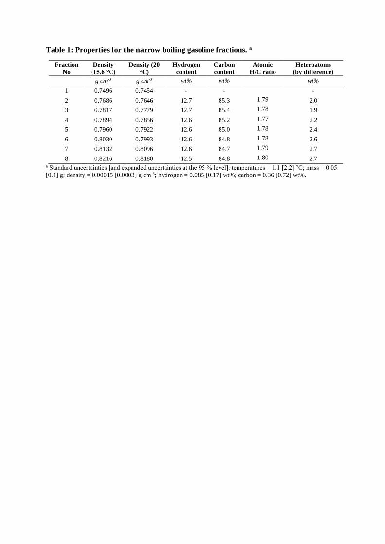
Table 1: Properties for the narrow boiling gasoline fractions. a

Fraction

No

Density

(15.6 °C)

Density (20

°C)

Hydrogen

content

Carbon

content

Atomic

H/C ratio

Heteroatoms

(by difference) g cm-3 g cm-3 wt% wt% wt%

1 0.7496 0.7454 - - -

2 0.7686 0.7646 12.7 85.3 1.79 2.0

3 0.7817 0.7779 12.7 85.4 1.78 1.9

4 0.7894 0.7856 12.6 85.2 1.77 2.2

5 0.7960 0.7922 12.6 85.0 1.78 2.4

6 0.8030 0.7993 12.6 84.8 1.78 2.6

7 0.8132 0.8096 12.6 84.7 1.79 2.7

8 0.8216 0.8180 12.5 84.8 1.80 2.7 a Standard uncertainties [and expanded uncertainties at the 95 % level]: temperatures = 1.1 [2.2] °C; mass = 0.05

[0.1] g; density = 0.00015 [0.0003] g cm-3; hydrogen = 0.085 [0.17] wt%; carbon = 0.36 [0.72] wt%.

Table 2: Accuracy of vapor pressures of benzene measured using the Eravap device.

Reference values were taken from NIST (Thermophysical Properties of Fluid Systems,

2017) and were based on an equation of state given by ´Polt et al. 1992´.

Temperature Vapor

pressure

Reference

value Difference

Difference

%

degC kPa kPa kPa %

40.0 25.0 24.36 0.6 97.4%

50.0 36.9 36.16 0.7 98.0%

60.0 53.2 52.19 1.0 98.1%

70.0 74.7 73.46 1.2 98.3%

80.0 102.8 101.06 1.7 98.3%

90.0 137.8 136.21 1.6 98.8%

100.0 181.0 180.20 0.8 99.6%

110.0 234.2 234.40 -0.2 100.1%

120.0 300.2 300.24 0.0 100.0%

Table 3: Measured vapor pressure data for the shale gasoline fractions. a

Temperature Fr. 1 Fr. 2 Fr. 3 Fr. 4 Fr. 5 Fr. 6 Fr. 7 Fr. 8

degC kPa kPa kPa kPa kPa kPa kPa kPa

30.0 15.1

37.2 36.8

37.8 38.4 19.9 11.4

40.0 41.5

50.0 57.7 31.4 12.8

60.0 78.8 43.9

70.0 105.6 37.2 27.2 19.7 15.7 11.8 8.1

80.0 139.0 80.8 51.2 28.2 22.5 15.4 11.5

90.0 180.1 69.2 52.9 39.6 30.7 21.6 16.5

100.0 91.7 70.1 53.9 41.8 29.9 23.1

110.0 92.2 71.8 56.2 40.2 31.6 a Standard uncertainty of the vapor pressures: 0.66 kPa. Expanded uncertainty at the 95 % level: 1.5 kPa.

Table 4: Regression parameters and normal boiling points for the shale gasoline

fractions.

Fraction B Heat of

vaporization

Normal

boiling point kJ mol-1 °C

1 14.5 ± 0.1 28.0 ± 0.3 69

2 14.6 ± 0.2 30.0 ± 0.5 88

3 15.0 ± 0.1 32.4 ± 0.2 103

4 15.2 ± 0.3 33.9 ± 0.7 113

5 15.4 ± 0.2 35.4 ± 0.7 122

6 14.9 ± 0.2 34.7 ± 0.6 132

7 14.4 ± 0.9 34 ± 3 147

8 15.2 ± 0.3 37.4 ± 0.7 152

Table 5: Comparison of the root mean squared errors (RMSE) of various correlations

when used for predicting the vapor pressures of the shale gasoline samples.

Correlation RMSE

(kPa) Reference

Van Kranen and Van

Nes 3.4 (Nes and Westen, 1951)

Maxwell and Bonnell 2.9 (Maxwell J. B. and Bonnell, 1955; Maxwell J. B.

and Bonnell, 1957)

Modified Maxwell and

Bonnell 2.9 (Wilson, 1981; Tsonopoulos et al., 1986)

Figure 1: Vapor pressures of the shale gasoline fractions on a 1/T vs. ln(P) plot.

Figure 2: Deviation of predicted vapor pressures from the experimental values.

Figure 3: Deviation of predicted vapor pressures via Maxwell and Bonnell equation from the

experimental values.