Measuring productivity - OECD
44
OECD Economic Studies No. 33, 2001/II 127 © OECD 2001 MEASURING PRODUCTIVITY Paul Schreyer and Dirk Pilat TABLE OF CONTENTS Introduction ................................................................................................................................. 128 Measuring productivity growth.................................................................................................. 129 Gross output and value-added based productivity measures ......................................... 129 Measuring output .................................................................................................................... 136 Labour input ............................................................................................................................ 138 Capital input ............................................................................................................................ 142 Index numbers ......................................................................................................................... 146 Estimating productivity levels .................................................................................................. 147 Output, labour and capital input........................................................................................... 148 Purchasing power parities for international comparisons.................................................. 150 Estimates of income and labour productivity levels.......................................................... 152 The interpretation of productivity measures .......................................................................... 157 The link with technological change ....................................................................................... 157 Productivity growth and changes in costs ............................................................................ 159 The role of the business cycle in productivity growth........................................................ 160 The difference between productivity and efficiency.......................................................... 160 How productivity at the industry level is related to that at the firm level ...................... 161 Innovation and productivity .................................................................................................. 162 In conclusion ................................................................................................................................ 163 Bibliography ................................................................................................................................ 166 National Accounts Division, Statistics Directorate, and Economic Analysis and Statistics Division, Direc- torate for Science, Technology and Industry, respectively. The authors are grateful for comments from Andrew Dean, Jørgen Elmeskov and Paul Swaim on an earlier draft.
-
Upload
khangminh22 -
Category
Documents
-
view
0 -
download
0
Transcript of Measuring productivity - OECD
OECD Economic Studies No. 33, 2001/II
127
© OECD 2001
MEASURING PRODUCTIVITY
Paul Schreyer and Dirk Pilat
TABLE OF CONTENTS
Introduction ................................................................................................................................. 128
Measuring productivity growth.................................................................................................. 129Gross output and value-added based productivity measures ......................................... 129Measuring output .................................................................................................................... 136Labour input ............................................................................................................................ 138Capital input ............................................................................................................................ 142Index numbers......................................................................................................................... 146
Estimating productivity levels .................................................................................................. 147Output, labour and capital input........................................................................................... 148Purchasing power parities for international comparisons.................................................. 150Estimates of income and labour productivity levels.......................................................... 152
The interpretation of productivity measures .......................................................................... 157The link with technological change....................................................................................... 157Productivity growth and changes in costs ............................................................................ 159The role of the business cycle in productivity growth........................................................ 160The difference between productivity and efficiency.......................................................... 160How productivity at the industry level is related to that at the firm level ...................... 161Innovation and productivity .................................................................................................. 162
In conclusion ................................................................................................................................ 163
Bibliography ................................................................................................................................ 166
National Accounts Division, Statistics Directorate, and Economic Analysis and Statistics Division, Direc-torate for Science, Technology and Industry, respectively. The authors are grateful for comments fromAndrew Dean, Jørgen Elmeskov and Paul Swaim on an earlier draft.
128
© OECD 2001
INTRODUCTION
Productivity growth is the basis for improvements in real incomes and wel-fare. Slow productivity growth limits the rate at which real incomes can improve,and also increases the likelihood of conflicting demands concerning the distribu-tion of income (Englander and Gurney, 1994). Measures of productivity growth andof productivity levels therefore constitute important economic indicators.
In principle, productivity is a rather straightforward indicator. It describes therelationship between output and the inputs that are required to generate thatoutput. Despite its apparent simplicity, several problems arise when measuringproductivity. These issues are particularly important for comparing productivitygrowth across countries, whether for the entire economy or for different industries,and for comparing productivity levels internationally. Some of these measurementdifficulties are closely related to technological developments – currently of greatinterest. For example, assessing the role of information and communication tech-nology (ICT) in productivity growth requires the construction of accurate price andquantity indices of ICT products that are internationally comparable. Other issues,such as the measurement of labour input, have been around for much longer, butremain important. The most important productivity measurement issues haverecently been brought together in the OECD Productivity Manual (OECD, 2001a) andpart of the discussion below draws on this manual.
There are many different measures of productivity growth. The choicebetween them depends on the purpose of productivity measurement and, inmany instances, on the availability of data. Broadly, productivity measures can beclassified as single-factor productivity measures (relating a measure of output to asingle measure of input) or multi-factor productivity measures (relating a measureof output to a bundle of inputs).1 Another distinction, of particular relevance at theindustry or firm level is between productivity measures that relate gross output toone or several inputs and those which use a value-added concept to capturemovements of output.
Table 1 uses these criteria to enumerate the main productivity measures. Thelist is incomplete insofar as single productivity measures can also be defined overintermediate inputs and labour-capital multi-factor productivity can, in principle,be evaluated on the basis of gross output. However, in the interest of simplicity,the table was restricted to the most frequently used productivity measures. These

Measuring Productivity
129
© OECD 2001
are measures of labour and capital productivity, and multi-factor productivitymeasures (MFP), either in the form of capital-labour MFP, based on a value-addedconcept of output, or in the form of capital-labour-energy-materials-services MFP(KLEMS), based on a concept of gross output. Among those measures, value-added-based labour productivity is the single most frequently computed produc-tivity statistic, followed by capital-labour MFP and KLEMS MFP.
A full discussion of the entire set of productivity measures would go beyondthe scope of this paper. The following pages will therefore highlight some key con-ceptual and measurement issues associated with comparisons of productivitygrowth and productivity levels over time and between countries. The sections onproductivity growth and on the interpretation of productivity measures draw heavilyon the OECD Productivity Manual (OECD, 2001a) to which the reader is referred for amore in-depth discussion. The paper primarily focuses on measurement and com-parability issues, leaving the detailed analysis and interpretation of productivity toother papers in this issue of OECD Economic Studies. The next section explores mea-sures of productivity growth and the theoretical foundations for these measures.The third section examines estimates of productivity levels, while the fourth sectionbriefly discusses the interpretation of productivity growth and levels.
MEASURING PRODUCTIVITY GROWTH
Gross output and value-added based productivity measures
Every productivity measure, implicitly or explicitly, relates to a specific pro-ducer unit: an establishment, a firm, an industry, a sector or an entire economy.The goods or services that are produced within a producer unit and that become
Table 1. Overview of the main productivity measures
Type of output measure:
Type of input measure
Labour Capital Capital and labour
Capital, labour and intermediate inputs
(energy, materials, services)
Gross output Labour productivity (based on gross
output)
Capital productivity (based on gross
output)
Capital – labour MFP (based on gross
output)
KLEMS multi-factor productivity
Value-added Labour productivity (based on value-
added)
Capital productivity (based on value-
added)
Capital – labour MFP (based on value-
added)
–
Single factor productivity measures Multi-factor productivity (MFP) measures
OECD Economic Studies No. 33, 2001/II
130
© OECD 2001
available for use outside the unit are called (gross) output.2 Output is producedusing primary inputs (labour and capital) and intermediate inputs. This relation isnormally presented as a production function H with gross output Q, labour inputL, capital input K, intermediate inputs M and a parameter of technical change, A:
Q = H (A, K, L, M) (1)
Technical change is called “Hicks-neutral” or “output augmenting” when it canbe presented as an outward shift of the production function that affects all factorsof production proportionately:
Q = H (A, K, L, M) = A • F (K, L, M) (2)
Differentiating this expression with respect to time and using a logarithmicrate of change, MFP growth (the rate of change of the variable A) is measured asthe rate of change of volume output minus the weighted rates of change of inputs.For a cost-minimising producer, the weights attached to the rates of change of fac-tor inputs correspond to the revenue share of each factor in total gross output:
Here, MFP growth is positive when the rate of growth of the volume of grossoutput rises faster than the rate of growth of all combined inputs. When theassumption about factor-augmenting technical change holds, the so computedMFP measure can be interpreted as an index of disembodied technical change.This is the well-known Solow (1959) growth accounting model (Box 1; Box 2).
However, the gross output based approach provides few insights about therelative importance of a firm or an industry for productivity growth of a larger (par-ent) sector or of the entire economy, due to complications related to intra-industrydeliveries. This is best explained by way of an example. Suppose that there aretwo industries: the leather industry, which only produces intermediate inputs forthe shoe industry. By contrast, the shoe industry produces only final output. A pro-ductivity measure for the aggregate shoe and leather industry would need to addressthe following problem. Simple addition of the flows of outputs and inputs is notthe right procedure for obtaining measures of output and input of the shoe andleather industry as a whole, since double counting of the intermediate flowsbetween the leather and the shoe producer would result. These flows have to benetted out, such that the output of the integrated shoe and leather industry wouldconsist only of the shoes produced, and integrated intermediate inputs consistonly of the purchases of the leather industry and non-leather purchases of theshoe industry. This has important consequences for productivity measures. Take
dt
Mds
dt
Kds
dt
Lds
dt
Qd
dt
AdMKL
lnlnlnlnln −−−= (3)
Measuring Productivity
131
© OECD 2001
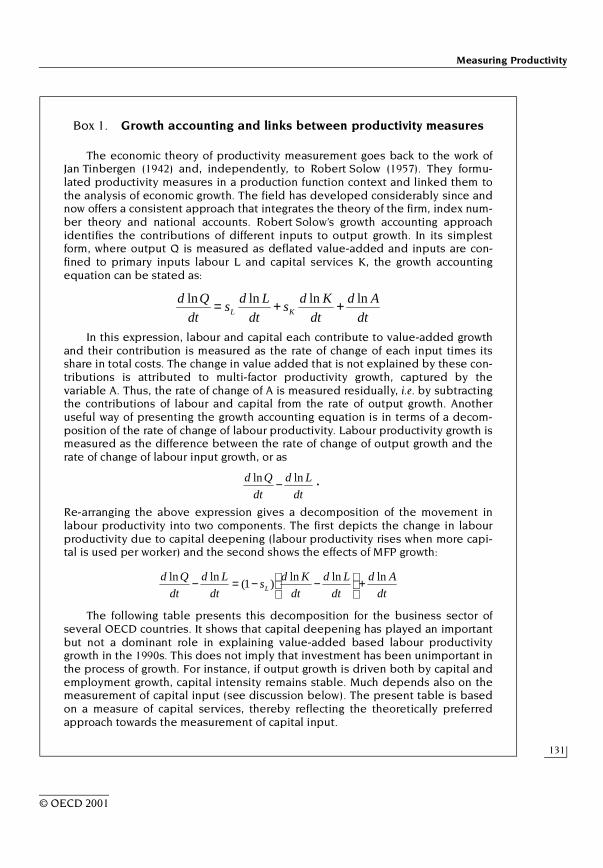
Box 1. Growth accounting and links between productivity measures
The economic theory of productivity measurement goes back to the work ofJan Tinbergen (1942) and, independently, to Robert Solow (1957). They formu-lated productivity measures in a production function context and linked them tothe analysis of economic growth. The field has developed considerably since andnow offers a consistent approach that integrates the theory of the firm, index num-ber theory and national accounts. Robert Solow’s growth accounting approachidentifies the contributions of different inputs to output growth. In its simplestform, where output Q is measured as deflated value-added and inputs are con-fined to primary inputs labour L and capital services K, the growth accountingequation can be stated as:
In this expression, labour and capital each contribute to value-added growthand their contribution is measured as the rate of change of each input times itsshare in total costs. The change in value added that is not explained by these con-tributions is attributed to multi-factor productivity growth, captured by thevariable A. Thus, the rate of change of A is measured residually, i.e. by subtractingthe contributions of labour and capital from the rate of output growth. Anotheruseful way of presenting the growth accounting equation is in terms of a decom-position of the rate of change of labour productivity. Labour productivity growth ismeasured as the difference between the rate of change of output growth and therate of change of labour input growth, or as
Re-arranging the above expression gives a decomposition of the movement inlabour productivity into two components. The first depicts the change in labourproductivity due to capital deepening (labour productivity rises when more capi-tal is used per worker) and the second shows the effects of MFP growth:
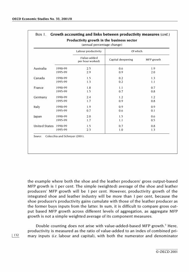
The following table presents this decomposition for the business sector ofseveral OECD countries. It shows that capital deepening has played an importantbut not a dominant role in explaining value-added based labour productivitygrowth in the 1990s. This does not imply that investment has been unimportant inthe process of growth. For instance, if output growth is driven both by capital andemployment growth, capital intensity remains stable. Much depends also on themeasurement of capital input (see discussion below). The present table is basedon a measure of capital services, thereby reflecting the theoretically preferredapproach towards the measurement of capital input.
dt
Ad
dt
Kds
dt
Lds
dt
QdKL
lnlnlnln ++=
dt
Ld
dt
Qd lnln − .
dt
Ad
dt
Ld
dt
Kds
dt
Ld
dt
QdL
lnlnln)1(
lnln +
−−=−
OECD Economic Studies No. 33, 2001/II
132
© OECD 2001
the example where both the shoe and the leather producers’ gross output-basedMFP growth is 1 per cent. The simple (weighted) average of the shoe and leatherproducers’ MFP growth will be 1 per cent. However, productivity growth of theintegrated shoe and leather industry will be more than 1 per cent, because theshoe producer’s productivity gains cumulate with those of the leather producer asthe former buys inputs from the latter. In sum, it is difficult to compare gross out-put based MFP growth across different levels of aggregation, as aggregate MFPgrowth is not a simple weighted average of its component measures.
Double counting does not arise with value-added-based MFP growth.3 Here,productivity is measured as the ratio of value-added to an index of combined pri-mary inputs (i.e. labour and capital), with both the numerator and denominator
Box 1. Growth accounting and links between productivity measures (cont.)
Productivity growth in the business sector(annual percentage change)
Source: Colecchia and Schreyer (2001).
Labour productivity Of which:
(Value-added per hour worked)
Capital deepening MFP growth
Australia 1990-99 2.5 0.6 1.91995-99 2.9 0.9 2.0
Canada 1990-99 1.5 0.2 1.31995-99 1.3 0.2 1.1
France 1990-99 1.8 1.1 0.71995-99 1.5 0.7 0.8
Germany 1990-99 2.4 1.2 1.21995-99 1.7 0.9 0.8
Italy 1990-99 1.9 0.9 0.91995-99 0.7 0.6 0.1
Japan 1990-99 2.0 1.5 0.61995-99 1.7 1.1 0.5
United States 1990-99 1.5 0.7 0.81995-99 2.3 1.0 1.3
Measuring Productivity
133
© OECD 2001
representing deflated (real) volumes. Value-added, which takes the role of theoutput measure, is gross output corrected for purchases of intermediate inputs. Interms of rates of change, real value-added can be defined4 as
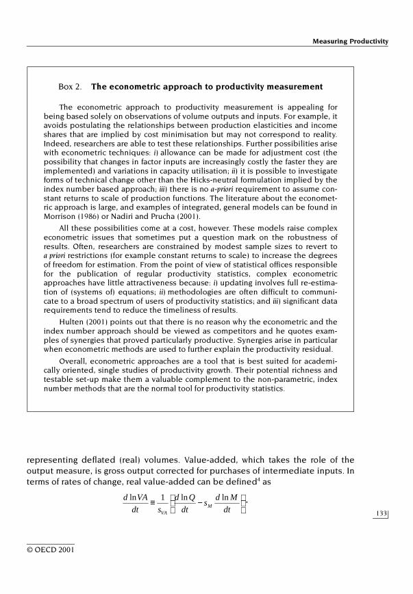
Box 2. The econometric approach to productivity measurement
The econometric approach to productivity measurement is appealing forbeing based solely on observations of volume outputs and inputs. For example, itavoids postulating the relationships between production elasticities and incomeshares that are implied by cost minimisation but may not correspond to reality.Indeed, researchers are able to test these relationships. Further possibilities arisewith econometric techniques: i) allowance can be made for adjustment cost (thepossibility that changes in factor inputs are increasingly costly the faster they areimplemented) and variations in capacity utilisation; ii) it is possible to investigateforms of technical change other than the Hicks-neutral formulation implied by theindex number based approach; iii) there is no a-priori requirement to assume con-stant returns to scale of production functions. The literature about the economet-ric approach is large, and examples of integrated, general models can be found inMorrison (1986) or Nadiri and Prucha (2001).
All these possibilities come at a cost, however. These models raise complexeconometric issues that sometimes put a question mark on the robustness ofresults. Often, researchers are constrained by modest sample sizes to revert toa priori restrictions (for example constant returns to scale) to increase the degreesof freedom for estimation. From the point of view of statistical offices responsiblefor the publication of regular productivity statistics, complex econometricapproaches have little attractiveness because: i) updating involves full re-estima-tion of (systems of) equations; ii) methodologies are often difficult to communi-cate to a broad spectrum of users of productivity statistics; and iii) significant datarequirements tend to reduce the timeliness of results.
Hulten (2001) points out that there is no reason why the econometric and theindex number approach should be viewed as competitors and he quotes exam-ples of synergies that proved particularly productive. Synergies arise in particularwhen econometric methods are used to further explain the productivity residual.
Overall, econometric approaches are a tool that is best suited for academi-cally oriented, single studies of productivity growth. Their potential richness andtestable set-up make them a valuable complement to the non-parametric, indexnumber methods that are the normal tool for productivity statistics.
−≡
dt
Mds
dt
Qd
sdt
VAdM
VA
lnln1ln .
OECD Economic Studies No. 33, 2001/II
134
© OECD 2001
Here, SVA stands for the current price share of value-added in gross output.Using equation (3) to substitute for the expression in parenthesis yields:
Value-added-based MFP measures, evaluated residually as the differencebetween the rate of change of real value-added and the weighted rates ofchange of primary inputs labour and capital, can then be expressed as in (5),where is the labour share in value-added and is the capitalshare.
Value-added-based MFP growth will be positive if volume value-added growsfaster than combined primary inputs. The advantage of the value-added measureis that aggregate value-added growth is a simple weighted average of value-added growth in individual industries, and so is value-added-based MFP growth.To stay with the above example, value added (at current prices) of the integratedshoe and leather industry is simply the sum of value-added in the shoe and theleather industry. A 1 per cent growth of value-added-based MFP in both the shoeand leather industry translates into a 1 per cent productivity growth of the shoeand leather industry as a whole. This makes value-added-based productivity mea-sures comparable across different levels of aggregation and turns them into mean-ingful indicators for an industry’s contribution to economy-wide productivitygrowth. Value-added is, however, not an immediately plausible measure of out-put: contrary to gross output, there is no physical quantity that corresponds to avolume measure of value added. Also, if the production model (2) is the “true”model of technical change, the value-added-based calculation will overstate5 therate of technical change, as
.
That is, the value-added-based MFP measure equals the gross output-basedmeasure times a scaling factor that corresponds to the inverted share of value-added in gross output. This share cannot exceed unity and consequently, thevalue-added-based MFP measure will always be at least as large as the gross out-put-based term.
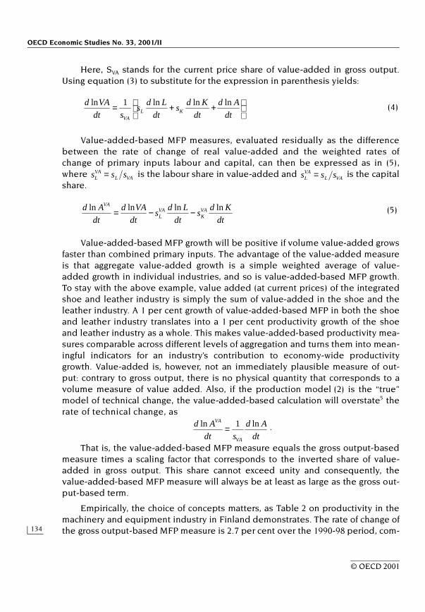
Empirically, the choice of concepts matters, as Table 2 on productivity in themachinery and equipment industry in Finland demonstrates. The rate of change ofthe gross output-based MFP measure is 2.7 per cent over the 1990-98 period, com-
++=
dt
Ad
dt
Kds
dt
Lds
sdt
VAdKL
VA
lnlnln1ln (4)
VALVAL sss = VAL
VAL sss =
dt
Kds
dt
Lds
dt
VAd
dt
Ad VAK
VAL
VA lnlnlnln −−= (5)
dt
Ad
sdt
Ad
VA
VA ln1ln =
Measuring Productivity
135
© OECD 2001
pared with a 7.8 per cent rise in the value-added-based measure. Moreover, thetwo measures show quite different pictures in terms of the acceleration or decelerationof productivity growth between two periods, an indicator that is of significantimportance to analysts as has been seen in the discussion about the “productivityslowdown” in the years after 1973 or the “productivity acceleration” in the UnitedStates in the late 1990s. In the Finnish example, the gross output-based measurerises from 2.1 per cent to 3.3 per cent per year between the first and the secondhalf of the 1990s, or by 1.2 percentage points; meanwhile, the value-added mea-sure rises from 5.7 per cent to 9.8 per cent, or by 4.1 percentage points.
In a closed economy, the difference between the two measures becomessmaller with a rising level of aggregation; at the level of the entire economy, thegross output-based productivity measure will equal the value-added based MFPmeasure. In an open economy, with imports from abroad, this is not the case andthe two measures will continue to produce different results even at the macroeco-nomic level.
Different interpretations have also to be invoked with respect to gross outputand value-added-based measures of labour productivity, both widely-used produc-tivity indices. Growth in value-added-based labour productivity depends on shiftsin capital intensity (the amount of capital available per unit of labour) and MFPgrowth. When measured as gross output per unit of labour input, labour productiv-ity growth also depends on how the ratio of intermediate inputs to labourchanges. A process of outsourcing, for example, implies substitution of primaryfactors of production, including labour, for intermediate inputs. Everything elseequal, gross output-based labour productivity rises as a consequence of outsourc-ing and falls when in-house production replaces purchases of intermediate inputs,
Table 2. Value-added and gross output-based productivity measures: an exampleMachinery and equipment industry, Finland
Averages of annual rates of change (percentages)
Source: OECD, based on STAN database.
1990-98 1990-94 1994-98
Gross output (deflated) 10.1 4.2 16.0Value added (deflated) 9.5 3.3 15.8
Labour input (total hours) 1.6 –3.7 6.9Capital input (gross capital stock) 3.0 1.5 4.5Intermediate inputs (deflated expenditure) 10.4 4.8 16.1
Share of value-added in gross output (current prices) 37.0 38.9 33.4
Gross output-based productivity (KLEMS MFP) 2.7 2.1 3.3Value-added based productivity (Capital-labour MFP) 7.8 5.7 9.8
OECD Economic Studies No. 33, 2001/II
136
© OECD 2001
despite the fact that such changes need not reflect changes in the individual char-acteristics of the workforce, nor shifts in technology or efficiency. By contrast, thegrowth rate of value-added productivity is less strongly affected by changes inthe ratio between intermediate inputs and labour, or the degree of vertical inte-gration. When outsourcing takes place, labour is replaced by intermediateinputs. In itself, this would raise measured labour productivity. At the sametime, however, value-added will fall, and this offsets some or the entire rise inmeasured productivity.
Overall, it would appear that gross output and value-added based productiv-ity measures are useful complements. When technical progress affects all factorsof production proportionally, the former is a better measure of technical change.Value-added-based productivity measures compensate for the extent of outsourc-ing and provide an indication of the importance of the productivity improvementin an industry for the economy as a whole. They indicate how much extra deliveryto final demand per unit of primary inputs an industry generates. When it comesto labour productivity, value-added based measures are less sensitive to changes inthe degree of vertical integration than gross output-based measures. Practicalaspects also come into play. Measures of value-added are often more easily avail-able than measures of gross output although in principle, gross output measuresare necessary to derive value-added data in the first place. Intra-industry flows ofintermediate products must be accounted for in order to generate consistent setsof gross output measures and that may be difficult empirically.
Measuring output
Differences in the methodologies used to obtain quantity series of output cansignificantly affect productivity measures. Quantity indices of output are normallyobtained by dividing a current-price series or index of output by an appropriateprice index (i.e. by deflation). Only in a few instances are quantity measuresderived by direct observation of volume output series.6 Measurement of volumeoutput is therefore often tantamount to constructing price indices – a task whosefull description far exceeds the scope of the present paper. Some of the more dif-ficult issues associated with the deflation of output are nevertheless mentionedhere.
Independence of measures of output from measures of input. An important pre-condition for the validity of productivity measures is that price and quantity indi-ces of output should be constructed independently of price and quantity indicesof inputs. Such dependence occurs, for example, when quantity indices of outputsare extrapolated using quantity indices for one or several inputs. The quantityindicators used are often inputs to the industry under consideration, in particularobservations on employment.
Measuring Productivity
137
© OECD 2001
In other instances, output-related measures are used to extrapolate realvalue-added. Though often imperfect, it is apparent that the implied bias for pro-ductivity measurement is less severe than in the case of input-based extrapola-tion. For example, Eldridge (1999) reports that, in the United States, the quantityindicator for auto insurance expenditure is the deflated value of premiums, wheredeflation itself is based on a component index of the CPI. In other instances, phys-ical output data are used as the quantity indicator; the United States quantityindicator for brokerage charges is based primarily on BEA estimates of ordersderived from volume data from the Security and Exchange Commission and tradesources (Eldridge, 1999).
From the perspective of productivity measurement, the independence of sta-tistics on inputs and outputs is key. Using input-based indicators to construct out-put series generates an obvious bias in productivity measures; productivitygrowth will reflect whatever assumption about productivity growth was made bystatisticians in constructing the output series (e.g. that labour productivity wasunchanged). Occurrences of input-based extrapolation are concentrated in activi-ties where market output prices are difficult to observe. For this reason, input-based extrapolation is more frequent and quantitatively more important for ser-vice industries than for other parts of the economy (see OECD, 1996b for a surveyof methods in OECD countries) and can lead to biased productivity measures.
Quality change. The rapid development of information and communicationtechnology products has brought to centre-stage two long-standing questions forthe construction of price indices: how to deal with quality changes of existinggoods and how to account for new goods.7 The distinction between these twoissues is blurred because it is unclear where to draw the borderline between a“truly” new good and a new variety of an existing good.8
Typically, statistical agencies derive price indices for products by observingprice changes of items in a representative sample. New products, quality changesand new variants are common phenomena in the observation of price changes ofitems and statistical offices have well-established procedures to deal with them.9
Unfortunately, these methods are not the same across countries and sometimesyield implausibly large differences. The most widely quoted case is price indicesfor information and communications technology products such as computers.Their prices decline by between 30 per cent per year in the United States, andabout 5 per cent per year in a number of European countries. Given the homoge-neity and international tradability of these products, it is likely that some of thedifferences are due to statistical methods rather than actual price developments.In the present context, the question arises: how much do these differences matterfor comparisons of measures of output?
OECD Economic Studies No. 33, 2001/II
138
© OECD 2001
Empirically, the answer to this question depends largely on the level ofaggregation at which the analysis is conducted. As shown in Schreyer (2001), theeffects of a greater quality adjustment of ICT price measures tend to be compara-tively small for the measurement of economy-wide productivity, and certainly notof a size to account for differences in measured productivity growth betweencountries. This is largely due to the fact that many ICT products are imported, anda different price measure not only affects measures of final consumption (andhence GDP) but also measures of imports, implying that some of the effects onmeasured GDP are offsetting. On the other hand, the effects on measured outputvolumes are without doubt significant for individual industries such as the officeequipment and computer industry. Similarly, measures of individual demandcomponents, in particular the volume of investment, may suffer from a lack ofcomparability unless similar methods are used between countries in their effortsto account for quality change in high-tech products. Measures of the volume ofinvestment are of direct importance for productivity analysis as they are importantelements in the construction of capital stock series (see section on capital inputbelow).
Labour input
Different measures of employment. In the spirit of production theory, labourinput for an industry is most appropriately measured as the quality-adjusted num-ber of hours actually worked. The simplest, though least recommended, measureof labour input is a head count of jobs or employees. Such a measure fails toreflect changes in average work time per employee, multiple job holding (whenthe number of employees is the measure), self-employment and the quality oflabour.
A first refinement to this measure is its extension to total employment, com-prising both wage and salary earners, and the self-employed (including contribut-ing family members). A second refinement is the conversion from simple job (orperson) counts to estimates of total “hours actually worked”. Rates of change ofthe number of persons employed differ from the rates of change of total hoursworked when the number of average hours worked per person shifts over time.Such shifts may be due to a move towards more paid vacations, shorter “normal”hours for full-time workers and greater use of part-time work. Moreover, hoursworked will also vary over the business cycle as labour demand rises and falls.These developments have taken place in many OECD countries and underline theimportance of choosing “hours actually worked” as the variable for labour input inproductivity measurement because it bears a closer relation to the amount of pro-ductive services provided by workers than simple head counts.
Measuring Productivity
139
© OECD 2001
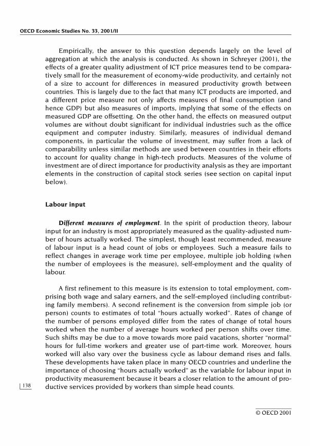
An example of the impact on labour productivity measures of choosing differ-ent measures for employment is given in Figure 1 below. For France, for theperiod 1987-98, labour productivity indices were calculated using total hours, thenumber of full-time equivalent persons, the number of employed persons (headcounts) and the number of employees (head counts). Results are presented forindustry (comprising mining, manufacturing and construction) and for market ser-vices. Not surprisingly, the productivity measures based on total hours rise signifi-cantly faster than those based on other employment measures. In manufacturing,moving from head counts to full-time equivalent measures hardly changes theproductivity series. This is quite different for the service sector where part-timeemployment has grown rapidly in many countries and now plays an important rolein total employment. Even more pronounced are the effects of including orexcluding the self-employed in the service sector, as reflected by the differences
Figure 1. Labour productivity1 based on different measures of employment in France
100
220
200
180
160
140
120
100
145
140
130
120
110
105
135
125
115
1978 80 82 84 86 88 90 92 94 96 98 1978 80 82 84 86 88 90 92 94 96 98
1. Output is measured as a quantity index of value-added.Source: INSEE.
Industry(mining, manufacturing and construction)
Market services
Value-added per hour: 3.7% per yearValue-added per employee(headcount): 3.3% per yearValue-added per person employed(headcount): 3.4% per yearValue-added per full-timeequivalent person: 3.4% per year
Value-added per hour: 1.8% per yearValue-added per employee(headcount): 1.0% per yearValue-added per person employed(headcount): 1.3% per yearValue-added per full-timeequivalent person: 1.5% per year
100
220
200
180
160
140
120
100
145
140
130
120
110
105
135
125
115
1978 80 82 84 86 88 90 92 94 96 98 1978 80 82 84 86 88 90 92 94 96 98
1. Output is measured as a quantity index of value-added.Source: INSEE.
Industry(mining, manufacturing and construction)
Market services
Value-added per hour: 3.7% per yearValue-added per employee(headcount): 3.3% per yearValue-added per person employed(headcount): 3.4% per yearValue-added per full-timeequivalent person: 3.4% per year
Value-added per hour: 1.8% per yearValue-added per employee(headcount): 1.0% per yearValue-added per person employed(headcount): 1.3% per yearValue-added per full-timeequivalent person: 1.5% per year
OECD Economic Studies No. 33, 2001/II
140
© OECD 2001
in productivity estimates based on total employment and based on the number ofemployees only.
Full-time equivalent jobs (or persons) are another variable sometimes usedfor measuring labour input. By definition, full-time equivalent employment is thenumber of total hours worked divided by average annual hours actually worked infull-time jobs. Conceptually, then, in full-time equivalent measures part-timeemployed persons are counted with a smaller weight than persons working fulltime. Consequently, the full-time equivalent measure should avoid the bias aris-ing from a shifting share of part-time employment in the workforce but will notadjust for changes in the number of hours which constitutes a full-time job, e.g. asa consequence of changes in legislation or collective agreements. In addition,methodologies underlying the construction of full-time equivalent persons (orjobs) are not always transparent and may vary internationally. For example, insome cases full-time equivalents are based on crude estimates, such as countingeach part-time job (often defined as any job with less than normal working hours)as half a full-time job.
Statistical sources. There are two main statistical sources for measures oflabour input: household-based labour force surveys (LFS) and establishment orfirm-based surveys (ES). LFS are typically conducted from a socio-economic per-spective to provide reliable information about personal characteristics of thelabour force, such as educational attainment, age, or the occurrence of multiplejob holding, as well as information about the jobs (e.g. occupation and type of con-tract). Also, LFS have the advantage of full coverage of the economy. ES are con-ducted from a production perspective, and describe labour as an input factor. Onedistinguishing feature of establishment surveys is that they gather information onjobs rather than on persons employed, thus persons who have jobs in more thanone establishment will be counted more than once. Another feature is that ES willoften only cover a subset of all establishments in an industry, normally thoseabove a certain size limit. If establishments included in the survey have systemat-ically higher productivity levels than those excluded, productivity estimatesbased on ES will inadequately reflect the effects of the size composition in anindustry.
In a few OECD countries (e.g. the Netherlands), statistical offices fully consoli-date the two sources into a single, final set of labour accounts. In most countries,both sources are used to construct employment data for national accounts (NA).As such, these NA data qualify as the preferred source for productivity analysis.However, NA statistics often stop short of producing all the relevant labour inputmeasures (in particular hours worked) or such variables are not available at therequired sectoral detail. In such cases, multiple sources sometimes have to becombined, although this introduces the risk of not comparing like with like. Onesuch example is the application of data on average hours worked per person,
Measuring Productivity
141
© OECD 2001
based on LFS, to NA-based statistics on the number of persons employed. Thismay be acceptable for purposes of constructing measures of productivity growthbut can create important non-comparabilities when measuring productivity levels(see below for a further discussion).
Skill composition of labour. Labour input reflects the time, effort and skills ofthe workforce. While data on hours worked capture the time dimension, they donot reflect the skill dimension. When total hours worked are the simple sum of allhours of all workers, no account is taken of the heterogeneity of labour. For theestimation of productivity changes, the question is whether, over time, the compo-sition of the labour force changes, i.e. whether there is an increase or decrease inthe average quality of labour input. By most measures, there has been a steadyincrease in the quality of labour (OECD, 1998a). An increase in the average qualityof labour implies that a quality-adjusted measure of labour input would rise fasterthan an unadjusted measure of labour input. Successful quality-adjustment is tan-tamount to measuring labour in constant-quality units. In the context of productiv-ity measurement, Jorgenson et al. (1987), Denison (1985) and the US Bureau ofLabor Statistics (BLS, 1993) have tackled this issue
Measuring constant-quality labour input is interesting from several perspec-tives. First, it provides a more accurate indication of the contribution of labour toproduction. One recalls that MFP measures the residual growth in output that can-not be explained by the rate of change in the services of labour, capital and inter-mediate inputs. When quality-adjusted measures of labour input are used ingrowth accounting instead of unadjusted hours worked, a larger share of outputgrowth will be attributed to the factor labour instead of the residual factor produc-tivity growth. In other words, substituting quality-adjusted labour input measuresfor unadjusted measures can better identify the sources of growth, by distinguish-ing between externalities or spill-overs – captured by the productivity residual –and the effects of investment in human capital.
Second, a comparison of an adjusted and unadjusted measure of labour inputyields a measure of the corresponding compositional or quality change of labourinput. This can usefully be interpreted as one aspect of the formation of humancapital, and is thus a step towards measuring the effects of intangible investment.
The theory of the firm stipulates that, under certain conditions (i.e. the firm isa price-taker on labour markets and minimises its total costs), labour of a certaintype will be hired up to the point where the cost of an additional hour of labour isjust equal to the additional revenue that using this labour generates. This equalityimplies that, for a measure of total labour input, the individual labour inputs ofdifferent quality can be weighted using their relative wage rates (or, more pre-cisely, the shares of each type of labour in total labour compensation).
OECD Economic Studies No. 33, 2001/II
142
© OECD 2001
Even when labour input is differentiated only by a simple trait, such as occu-pation, information requirements are severe: data are needed that distribute thenumber of total hours worked across different occupations, by individual industryand by individual year. In addition, quantity measures of labour input (i.e. hoursworked) have to be accompanied by price measures (i.e. relative average compen-sation) to construct weights for aggregation. Such rich data sets are normally bothdifficult and costly to collect and therefore not readily available in practice.10
Even when such data are not available, “implicit differentiation” can providea useful, albeit incomplete, adjustment for labour quality. Implicit differentiationarises when labour input (i.e. total hours worked) is measured by detailed industrywithout, however, distinguishing between different types of labour within eachindustry. If the rate of change in hours worked by industry are aggregated to theeconomy-wide level using each industry’s share in total labour compensation asits aggregation weight, these weights will be relatively large for industries that payabove-average wages and relatively small for industries with below-averagewages. Assuming that above-average wages reflect an above-average skill compo-sition of the workforce, some of the quality change of labour input is implicitlytaken into account. Statistics Canada’s industry-level productivity statistics pro-vide an example of implicit differentiation, since the indices of labour input at thesectoral level are built up from hours-worked data for more detailed industriesthat are weighted by their shares in total sectoral labour compensation.
Capital input
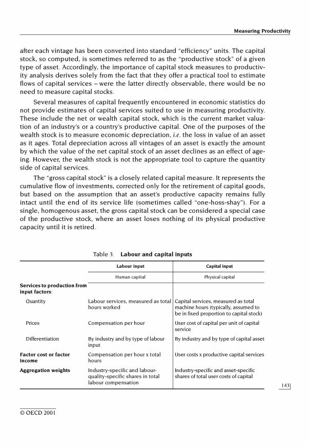
In a production process, labour, capital and intermediate inputs are com-bined to produce one or several outputs. Conceptually, many facets of capitalinput measurement are directly analogous to labour input measurement (Table 3).Capital goods, whether purchased or rented by a firm, provide a flow of capitalservices that constitutes the actual input to the production process. Similarly,employees hired for a certain period can be seen as providing flows of labour ser-vices from their stocks of human capital. Differences between labour and capitalarise because producers usually own capital goods. When the capital good “deliv-ers” services to its owner, no market transaction is recorded. The measurement ofthese implicit transactions – whose quantities are the services drawn from thecapital stock during a period and whose prices are the user costs or rental pricesof capital – is one of the challenges of capital measurement.
Constructing measures of capital services.11 Conceptually, capital servicesreflect a quantity or physical concept that should not to be confused with thevalue or price concept of capital. Because flows of the quantity of capital servicesare not usually directly observable, they have to be approximated. Most often,this is done by assuming that service flows are in proportion to the stock of assets,
Measuring Productivity
143
© OECD 2001
after each vintage has been converted into standard “efficiency” units. The capitalstock, so computed, is sometimes referred to as the “productive stock” of a giventype of asset. Accordingly, the importance of capital stock measures to productiv-ity analysis derives solely from the fact that they offer a practical tool to estimateflows of capital services – were the latter directly observable, there would be noneed to measure capital stocks.
Several measures of capital frequently encountered in economic statistics donot provide estimates of capital services suited to use in measuring productivity.These include the net or wealth capital stock, which is the current market valua-tion of an industry’s or a country’s productive capital. One of the purposes of thewealth stock is to measure economic depreciation, i.e. the loss in value of an assetas it ages. Total depreciation across all vintages of an asset is exactly the amountby which the value of the net capital stock of an asset declines as an effect of age-ing. However, the wealth stock is not the appropriate tool to capture the quantityside of capital services.
The “gross capital stock” is a closely related capital measure. It represents thecumulative flow of investments, corrected only for the retirement of capital goods,but based on the assumption that an asset’s productive capacity remains fullyintact until the end of its service life (sometimes called “one-hoss-shay”). For asingle, homogenous asset, the gross capital stock can be considered a special caseof the productive stock, where an asset loses nothing of its physical productivecapacity until it is retired.
Table 3. Labour and capital inputs
Labour input Capital input
Human capital Physical capital
Services to production from input factors:
Quantity Labour services, measured as total hours worked
Capital services, measured as total machine hours (typically, assumed to be in fixed proportion to capital stock)
Prices Compensation per hour User cost of capital per unit of capital service
Differentiation By industry and by type of labour input
By industry and by type of capital asset
Factor cost or factor income
Compensation per hour x total hours
User costs x productive capital services
Aggregation weights Industry-specific and labour-quality-specific shares in total labour compensation
Industry-specific and asset-specific shares of total user costs of capital
OECD Economic Studies No. 33, 2001/II
144
© OECD 2001
In empirical applications, the growth rate of capital services typically exceedsthat of the wealth stock. Using the wealth stock as a measure of capital input inproductivity calculations would thus imply an overstatement of MFP growth com-pared with the MFP associated with capital services (see below). On the otherhand, gross capital stock measures in productivity calculations potentially lead toan understatement of MFP growth, as gross stocks grow more rapidly than capitalservices.
The price of capital services is measured by their rental price. If there werecomplete markets for capital services, rental prices could be directly observed. Inthe cases of, for example, office buildings or cars, rental prices do exist and areobservable in the market. However, this is not the case for many other capitalgoods that are owned by producers and for which rental prices have to beimputed. The implicit rent that capital good owners “pay” themselves gives rise tothe terminology “user costs of capital”.
Because many different types of capital goods are used in production, anaggregate measure of the capital stock or of capital services must be constructed.For net (wealth) stocks this is a straightforward matter of summing estimates fordifferent types of assets. In so doing, market prices serve as aggregation weights.The situation is different in productivity analysis. Typically, each type of asset isassociated with a specific flow of capital services and strict proportionality isassumed between capital services and capital stocks at the level of individualassets. This ratio is not the same, however, for different kinds of assets, so that theaggregate stock and the flows covering different kinds of assets must diverge. Asingle measure cannot serve both purposes except when there is only one singlehomogenous capital good (Hill, 1999a).
Under competitive markets and equilibrium conditions, user costs reflect themarginal productivity of the different assets. User cost weights thus provide ameans to effectively incorporate differences in the productive contribution of het-erogeneous investments as the composition of investment and capital changes.Jorgenson (1963) and Jorgenson and Griliches (1967) were the first to developaggregate capital service measures that take the heterogeneity of assets intoaccount. They defined the flow of quantities of capital services individually foreach type of asset, and then applied asset-specific user costs as weights to aggre-gate across services from the different types of assets.
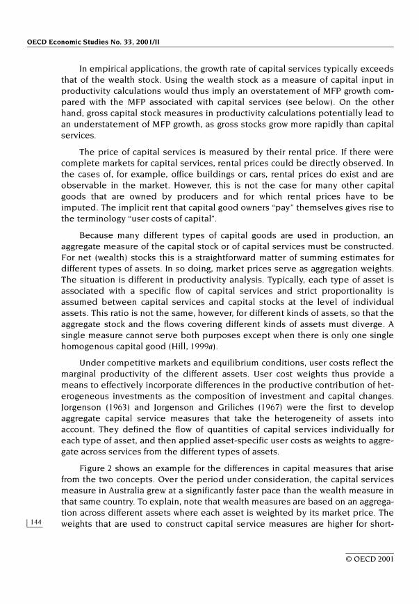
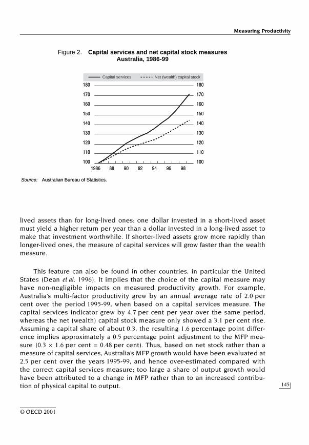
Figure 2 shows an example for the differences in capital measures that arisefrom the two concepts. Over the period under consideration, the capital servicesmeasure in Australia grew at a significantly faster pace than the wealth measure inthat same country. To explain, note that wealth measures are based on an aggrega-tion across different assets where each asset is weighted by its market price. Theweights that are used to construct capital service measures are higher for short-
Measuring Productivity
145
© OECD 2001
lived assets than for long-lived ones: one dollar invested in a short-lived assetmust yield a higher return per year than a dollar invested in a long-lived asset tomake that investment worthwhile. If shorter-lived assets grow more rapidly thanlonger-lived ones, the measure of capital services will grow faster than the wealthmeasure.
This feature can also be found in other countries, in particular the UnitedStates (Dean et al. 1996). It implies that the choice of the capital measure mayhave non-negligible impacts on measured productivity growth. For example,Australia’s multi-factor productivity grew by an annual average rate of 2.0 percent over the period 1995-99, when based on a capital services measure. Thecapital services indicator grew by 4.7 per cent per year over the same period,whereas the net (wealth) capital stock measure only showed a 3.1 per cent rise.Assuming a capital share of about 0.3, the resulting 1.6 percentage point differ-ence implies approximately a 0.5 percentage point adjustment to the MFP mea-sure (0.3 × 1.6 per cent = 0.48 per cent). Thus, based on net stock rather than ameasure of capital services, Australia’s MFP growth would have been evaluated at2.5 per cent over the years 1995-99, and hence over-estimated compared withthe correct capital services measure; too large a share of output growth wouldhave been attributed to a change in MFP rather than to an increased contribu-tion of physical capital to output.
Figure 2. Capital services and net capital stock measures Australia, 1986-99
100
170
140
120
110
150
130
180
160
100
170
140
120
110
150
130
180
160
1986 88 90 92 94 96 98
Source: Australian Bureau of Statistics.
Capital services Net (wealth) capital stock
100
170
140
120
110
150
130
180
160
100
170
140
120
110
150
130
180
160
1986 88 90 92 94 96 98
Source: Australian Bureau of Statistics.
Capital services Net (wealth) capital stock
OECD Economic Studies No. 33, 2001/II
146
© OECD 2001
Capital and capacity utilisation. There are many reasons why the rate of utilisa-tion of capital, or more generally, the rate of utilisation of capacity of a firm variesover time: a change in demand conditions, seasonal variations, interruptions inthe supply of intermediate products or a breakdown of machinery are all exam-ples of factors that lead to variations in the flow of capital services drawn from astock of assets. And yet, it is frequently assumed (for want of better information onutilisation rates) that the flow of services is a constant proportion of the capitalstock. This is one of the reasons for the pro-cyclical behaviour of productivityseries: variations in output are reflected in the data series, but the correspondingvariations in the utilisation of capital (and labour) inputs are inadequately cap-tured. If machine hours were measured, adjustments could be made. However, inpractice, the required data rarely exist and consequently, swings in demand andoutput are picked up by the residual productivity measure. There have been sev-eral attempts to deal with this issue, but a generally accepted solution has yet tobe found.
Index numbers
Productivity is usually measured as the ratio of a quantity index of output to aquantity index of inputs. Indices are required because the heterogeneity of goodsand services does not permit simply adding up units of different types of com-modities. However, aggregation results are in general sensitive to the choice of aspecific index number formula. These formulae should therefore be chosen care-fully on both conceptual and practical grounds.
A first choice that must be made for comparisons over several periods iswhether to compare two periods directly (say, between period 0 and period 2), orindirectly (in which case the change between period 0 and 2 is derived from thechange between period 0 and 1, combined with that from period 1 to 2). The eco-nomics literature, as well as the 1993 System of National Accounts, are quite unan-imous that inter-temporal comparisons over longer periods should be obtainedby chaining, i.e. by linking the year-to-year movements. The main reason for chain-ing is that it allows one to adopt weights that reflect economic behaviour: forexample, a relative price fall of a good will typically lead to higher consumption ofthis good and changes in the expenditure share of this item. Chained indicesreflect such changes in expenditure patterns because weights are regularlyupdated. When indices are based on weights that only reflect conditions in a baseperiod that is several years away from the comparison period, there is a risk ofweights being out of date and this may introduce a bias into the price or volumemeasure.
A second choice pertains to the specific index number formula. The mostwidely used index number formulae are the Laspeyres and Paasche indices (the
Measuring Productivity
147
© OECD 2001
former uses base-period weights, the latter current period weights), the Fisherindex (a geometric average of the Laspeyres and Paasche indices) and the Törn-qvist index (a weighted geometric average of its components).
To help decide between different index number formulae, a series of intu-itively appealing criteria have been developed in the index number literature,starting with the impressive work by Irving Fisher (1922). Examples of such criteriaare the identity test (if the prices of period 1 are the same as those of period 0, thenthe price index should take a value of one) or the commensurability test (the priceindex should be independent of the units of measurement). Many other criteriaexist (see Balk, 1995 for a survey), and the different index number formulae can bechecked against them.
Another approach makes use of economic theory to define price or quantityindices theoretically. A well-known example is the Konüs (1924) cost of livingindex derived from the micro-economic theory of the consumer. It is representedas the ratio of the minimum expenditure in period 1 over minimum expenditure inperiod 0, while maintaining utility constant. Empirically, it is not normally possibleto measure such a theoretically defined index directly as the specific form andparameters of utility or cost functions are unknown. However, Diewert (1976)showed that there are functional forms (such as the translog functional form) thatprovide approximations to arbitrary, twice differentiable homogenous functions.He further showed that these functional forms can be exactly represented by cer-tain index number formulae that he called “superlative” index numbers. This pro-vides a strong economic rationale for the use of superlative index numbers, suchas the Fisher and the Törnqvist index. Empirically, it turns out the choice betweendifferent types of superlative indices matters little and can thus be left to the indi-vidual researcher.
ESTIMATING PRODUCTIVITY LEVELS
International comparisons of productivity growth can give useful insights ingrowth processes, but should ideally be complemented with international com-parisons of income and productivity levels. An examination of levels gives insightsinto the possible scope for further gains, and also places a country’s growth experi-ence in the perspective of its current level of income and productivity. OECD haspublished estimates of productivity levels in various studies (e.g. Englander andGurney, 1994; Pilat, 1997; Scarpetta, et al., 2000). Most of these studies have notlooked in detail at measurement issues, or examined how differences in produc-tivity levels should be interpreted.
International comparisons of productivity levels require three components,namely comparable information on output (typically GDP), comparable informa-
OECD Economic Studies No. 33, 2001/II
148
© OECD 2001
tion on factor inputs (labour, capital) and conversion factors (or purchasing powerparities, PPPs) to translate output and factor inputs in national currencies to acommon currency. This section discusses the available estimates and some of themain measurement issues, in particular the use of PPPs for currency conversions,as well as the correspondence between output and labour input measures forlevel comparisons. The discussion focuses on productivity at the aggregate level.The estimation of sectoral productivity levels raises additional measurementissues that go beyond the scope of this paper.12
Output, labour and capital input
Comparability of output measures
The measurement and definition of economic output is treated systematicallyacross countries in the 1993 System of National Accounts (SNA 93). The revisionsto the SNA introduced at that time tend to increase the level of total GDP,although not uniformly over time or across countries. The SNA revisions raised thelevel of GDP in all of the OECD countries who have implemented these changes,with the increases ranging from 0.3 per cent for Belgium’s 1996 GDP, to 7.4 per centfor Korea’s 1996 GDP (Scarpetta, et al., 2000). Although most OECD countries havenow implemented the new SNA, Switzerland and Turkey are exceptions. Thus,GDP (and consequently productivity) levels in these countries are likely to beunderestimated compared with countries that have implemented the new system,although the extent of this bias is unknown. Once the introduction of the new SNAis completed, international comparability is likely to have improved.
A second factor that may influence the comparability of GDP across countriesis size of the non-observed economy. In principle, GDP estimates in the nationalaccounts take account of this part of the economy. In practice, questions can beraised about the extent to which official estimates have full coverage of economicactivities that are included in GDP according to the SNA, or to which extent mis-reporting is involved. Large differences in coverage could substantially affect com-parisons of productivity levels. Little is known about the possible size of the non-observed economy in different OECD member countries, although work is cur-rently underway to address this issue (OECD, 2000).
Comparability of labour-input measures
Equally important for international comparisons of productivity levels arecomparable measures of labour input. Labour input is commonly measured alongthree dimensions: the number of persons engaged; the total number of hoursworked of all persons engaged; and the total number of hours worked adjusted forthe quality of individual workers. Employment statistics are quite well standard-
Measuring Productivity
149
© OECD 2001
ised across OECD countries as most countries provide labour force statistics alongagreed guidelines. In principle, therefore, they pose few problems for interna-tional comparisons. The main difficulty is to ensure that the employment data areconsistent in coverage with other data that are required to make comparisons ofproductivity, notably GDP and hours worked.
There are two issues that arise here. The first question is whether countriesintegrate estimates of employment in the national accounts. These estimatescould be based on different sources, such as labour force surveys and enterprisestatistics, and would, in principle, be more consistent with GDP than estimatesrelying on only one single source. In practice, not all OECD countries integrateemployment statistics in the national accounts, implying that labour force statis-tics remain the most comparable source.
The second, closely related, problem is whether estimates of hours worked areconsistent with the employment data. Estimates of hours worked are typicallybased on two alternative sources, labour force surveys and enterprise statistics.Labour force surveys are based on surveys of households, whereas enterprise statis-tics survey firms. Both sources seem to have some advantages and disadvantagesfor comparisons of productivity levels (OECD, 1999a; Van Ark and McGuckin, 1999):
• Labour force surveys may underestimate absences due to illness and holidays.
• Evidence on time use related to labour force surveys suggests that personswho work long hours may overestimate their working time.
• Labour force surveys potentially pick up extra hours worked by managersand professionals that are over and above the conventional hours of work inan establishment and that are clearly not picked up by establishmentsources.
• Enterprise statistics are less likely to provide full coverage of all personsengaged in the economy, and may underestimate overtime.
In principle, this suggest that labour force surveys may somewhat overesti-mate total hours worked, whereas enterprise surveys may underestimate hoursworked. Much depends on the quality and coverage of the surveys, however, andseveral OECD countries provide comprehensive estimates of hours worked basedon a mix of sources. The OECD has recently produced estimates of hours workedthat draw on such a mix of sources, where hours worked estimates from labourforce surveys were adjusted downwards to compensate for known biases (Scar-petta, et al., 2000). Cross-country comparability can thus be improved as comparedto the use of original national sources for some countries, but there remains a mar-gin of uncertainty.
The quality of labour input is much more difficult to compare across coun-tries, in particular in terms of levels. Education systems and standards differ con-
OECD Economic Studies No. 33, 2001/II
150
© OECD 2001
siderably across countries, information on firm-level training is not collected orincomplete in most countries, and reliable data are scarce in all these areas. Whilesome efforts have been made – primarily at the level of individual sectors – toaccount for qualitative differences in labour input across countries, the statisticalbasis is limited, and the results are therefore not necessarily robust.13 The OECDhas therefore not yet estimated quality-adjusted levels of labour input for interna-tional comparisons of productivity levels. The decomposition of GDP per capitabelow therefore ignores quality aspects of labour input in the estimation of labourproductivity levels.
Comparability of capital-input measures
Estimates of labour productivity levels are quite common. Much more diffi-cult and more controversial is the comparison of levels of capital productivity andof multi-factor productivity.14 The main controversy concerns the comparison ofcapital input across countries (Van Ark, 1996). Official estimates of capital stockembody a wide variety of assumed asset lives and retirement patterns.15 Some ofthe variation across countries may be accounted for by compositional differencesand differences in technological progress, which cause the capital stock to becomeobsolete more rapidly in some countries. However, this is difficult to verify and inmost cases the statistical basis for the variation in asset lives and retirement pat-terns is weak, since statistical offices collect such information only infrequently.
A second problem concerns the conversion of capital stocks in national currencyvalues into a common currency. This requires PPPs for capital stock. In principle, thesecan be derived from official PPPs for investment by converting investment series to acommon currency and then calculating capital stock in a common currency. Thisrequires reliable PPPs for investment and deflators for investment. PPPs for invest-ment have been criticised in some recent evaluations of the PPP programme (OECD,1997), however, and it is therefore not clear how reliable they are. Further progress isneeded in making capital stocks more comparable across countries so as to improvethe basis for comparisons of capital and multi-factor productivity.16
Purchasing power parities for international comparisons
The comparison of income and productivity across countries also requires pur-chasing power parity (PPP) data for GDP. Exchange rates are not suitable for the con-version of GDP to a common currency, since they do not reflect international pricedifferences, and since they are heavily influenced by short-term fluctuations. Overthe past two decades, OECD has regularly published estimates of PPPs, derivedfrom its joint programme with Eurostat. Benchmark estimates of PPPs are currentlyavailable for 1980, 1985, 1990, 1993 and 1996, and work is underway for a new bench-mark comparison for 1999.17 In using these PPP estimates for international compari-
Measuring Productivity
151
© OECD 2001
sons of income and productivity, two issues must be addressed, namely the choiceof aggregation method and the choice of benchmark year.
Aggregation method
The choice of aggregation method for constructing PPPs has been a source ofdebate over the past two decades. Initial work on international comparisons, suchas the seminal study by Kravis, Heston and Summers (1982), provided a widerange of aggregation methods. The latest benchmark comparisons by OECD andEurostat offer only two alternatives, namely those based on the Geary-Khamis(GK) method, and those based on the Elteto-Koves-Szulc (EKS) method.18 Aggre-gation takes place after price ratios for individual goods and services have beenaveraged to obtain unweighted parities for small groups of homogeneous com-modities. It involves weighting and aggregating the unweighted commodity groupparities to arrive at PPPs and real values for each category of expenditure up tothe level of total GDP.
The two methods differ substantially. The EKS method treats countries as aset of independent units with each country being assigned equal weight. The EKSprices are obtained by minimising the differences between multilateral binaryPPPs and bilateral binary PPPs. The EKS PPPs are thus close to the PPPs thatwould have been obtained if each pair of countries had been compared individu-ally. The GK method treats countries as members of a group. Each country isweighted according to its share in GDP and the prices that are calculated are char-acteristic of the group overall. Both methods have advantages and disadvantages:
• For countries with price structures that are very different from the average,the GK approach leads to higher estimates of volumes (and GDP per capita)than if more characteristic prices would have been used. This effect is par-ticularly important when comparing countries with great differences inincome levels. The GK approach leads to results that are additively consis-tent, however, which implies that the real value of aggregates is the sum ofthe real value of its components. This is an advantage for national accountsand permits comparisons of price and volume structures across countries.
• The EKS method leads to results that are more characteristic of each coun-try’s own prices, and thus leads to estimates of GDP per capita that are rela-tively similar to those resulting from the use of characteristic prices. Itsresults are not additive, however.
For OECD countries, the differences between the two methods are relativelysmall, since national price structures are similar. Most comparisons of income andproductivity utilise the EKS results, however, since these do not seem to overesti-mate income levels for low-income economies and are more closely aligned with
OECD Economic Studies No. 33, 2001/II
152
© OECD 2001
index number theory.19 The EKS method is also the method officially accepted byEurostat for administrative purposes.
Benchmark year
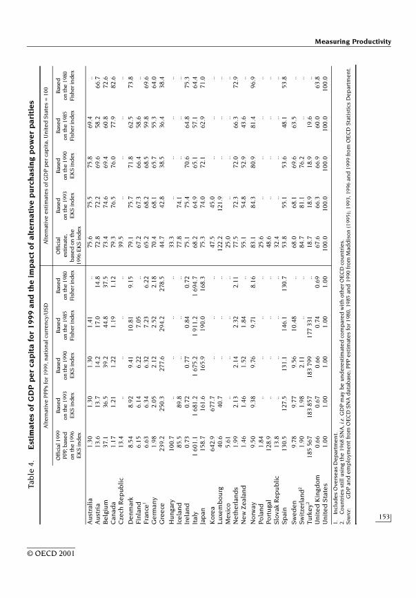
The second issue to be addressed concerns the choice of benchmark year.For several OECD countries, the OECD/Eurostat estimates of PPPs are currentlyavailable for five benchmark years. This raises a problem of which benchmark tochoose for international comparisons. In principle, it seems appropriate to use themost recent benchmark, i.e. 1996, since this is most likely to reflect current pricedifferences in the OECD area. To indicate the sensitivity of comparisons of incomeand productivity to the choice of benchmark, Table 4 provides an overview ofcomparative estimates of GDP per capita for 1999, based on alternative bench-mark results. It suggests that there is some variation in results between the differ-ent benchmark years, but that there are relatively small differences in resultsbetween recent benchmark years, i.e. 1990, 1993 and 1996. For most countries,the 1996 benchmark gives slightly higher estimates of GDP per capita relative tothe United States than the 1993 benchmark. France, Belgium, Norway and Spainare exceptions and have slightly lower levels of GDP per capita with the 1996benchmark.
Estimates of income and labour productivity levels
Clearly, data for international comparisons of income and productivity are notperfect and some choices between different sources have to be made. In thispaper, GDP is derived from the OECD SNA database, which incorporates the latestcomparative information on GDP from OECD member countries. Data on employ-ment are from the OECD Labour Force Statistics, as this source is more standardisedacross countries than employment data from the national accounts and since theestimates of hours worked that are used in this paper are closely linked to labourforce surveys. To convert GDP to a common currency, this paper uses the 1996benchmark PPPs as the most recently available.
Table 5 presents the resulting income and productivity level estimatesfor 1999. It shows a considerable diversity in real per-capita GDP levels across theOECD countries. The United States is at the top of the OECD income distribution,followed by Switzerland and Norway that have levels of GDP per capita between80 and 90 per cent of the US level. Luxembourg also has a very high level of GDPper capita, which is partly due to the large share of frontier workers in totalemployment (56 000 out of 226 000 workers in 1997). These contribute to GDPand employment, but are not included in the working-age and total population.The bulk of the OECD, including all the other major economies, has income lev-els that are between 65 and 80 per cent of the US level. Following this group are
Measuring Productivity
153
© OECD 2001
Tab
le 4
. E
stim
ate
s o
f G
DP
pe
r ca
pit
a fo
r1
99
9 a
nd t
he
im
pa
ct o
f a
lter
na
tive
pu
rch
asi
ng
po
we
r p
ari
tie
s
1.In
clu
de
s O
vers
eas
De
par
tme
nt.
2.C
ou
ntr
ies
stil
l usi
ng
the
1968
SN
A, i
.e.G
DP
may
be
un
de
rest
imat
ed
co
mp
are
d w
ith
oth
er
OE
CD
co
un
trie
s.S
ourc
e:
GD
P a
nd
em
plo
yme
nt
fro
m O
EC
D S
NA
dat
abas
e; P
PP
est
imat
es
for
1980
, 198
5 an
d19
90 fr
om
Mad
dis
on
(19
95);
199
3, 1
996
and
1999
fro
m O
EC
D S
tati
stic
s D
ep
artm
en
t.
Alt
ern
ativ
e P
PP
s fo
r19
99, n
atio
nal
cu
rre
ncy
/US
DA
lte
rnat
ive
est
imat
es
of G
DP
pe
r ca
pit
a, U
nit
ed
Sta
tes
= 1
00
Offi
cial
1999
P
PP, b
ase
d
onth
e19
96
EK
S in
dex
Bas
ed
on
the
1993
E
KS
ind
ex
Bas
ed
o
nth
e19
90
EK
S in
de
x
Bas
ed
on
the
1985
F
ish
er in
de
x
Bas
ed
onth
e19
80
Fish
er i
nd
ex
Offi
cial
es
tim
ate,
b
ase
d o
n th
e 19
96 E
KS
ind
ex
Bas
ed
on
the
1993
E
KS
ind
ex
Bas
ed
onth
e19
90
EK
S in
dex
Bas
ed
on
the
1985
Fi
she
r in
dex
Bas
ed
o
nth
e19
80
Fish
er in
de
x
Au
stra
lia
1.30
1.30
1.30
1.41
..75
.675
.575
.869
.4..
Au
stri
a13
.613
.714
.217
.014
.872
.872
.269
.658
.266
.7B
elg
ium
37.1
36.5
39.2
44.8
37.5
73.4
74.6
69.4
60.8
72.6
Can
ada
1.17
1.21
1.22
1.19
1.12
79.3
76.5
76.0
77.9
82.6
Cze
ch R
ep
ub
lic
13.4
....
....
39.5
....
....
De
nm
ark
8.54
8.92
9.41
10.8
19.
1579
.175
.771
.862
.573
.8F
inla
nd
6.15
6.14
6.22
7.05
..67
.267
.366
.458
.6..
Fra
nce
16.
636.
346.
327.
236.
2265
.268
.268
.559
.869
.6G
erm
any
1.98
2.05
2.12
2.52
2.18
70.4
68.1
65.7
55.3
64.0
Gre
ece
239.
225
0.3
277.
629
4.2
278.
544
.742
.838
.536
.438
.4
Hu
nga
ry10
0.7
....
....
33.3
....
....
Ice
lan
d85
.589
.8..
....
77.8
74.1
....
..Ir
ela
nd
0.73
0.72
0.77
0.84
0.72
75.1
75.4
70.6
64.8
75.3
Ital
y1
601.
11
681.
21
675.
21
911.
21
694.
768
.264
.965
.157
.164
.4Ja
pan
158.
716
1.6
165.
919
0.0
168.
375
.374
.072
.162
.971
.0
Ko
rea
642.
967
7.7
....
..47
.545
.0..
....
Lu
xem
bo
urg
40.6
40.7
....
..12
2.2
121.
9..
....
Me
xico
5.61
....
....
25.0
....
....
Ne
the
rlan
ds
1.99
2.13
2.14
2.32
2.11
77.5
72.3
72.0
66.3
72.9
Ne
w Z
eal
and
1.46
1.46
1.52
1.84
..55
.154
.852
.943
.6..
No
rway
9.50
9.38
9.76
9.71
8.16
83.1
84.3
80.9
81.4
96.9
Po
lan
d1.
84..
....
..25
.6..
....
..P
ort
uga
l12
8.9
....
....
48.6
....
....
Slo
vak
Re
pu
bli
c13
.8..
....
..32
.4..
....
..S
pai
n13
0.5
127.
513
1.1
146.
113
0.7
53.8
55.1
53.6
48.1
53.8
Sw
ed
en
9.78
9.77
9.56
10.4
8..
68.0
68.1
69.6
63.5
..S
wit
zerl
and
21.
901.
982.
11..
..84
.781
.176
.2..
..Tu
rke
y218
5 56
718
3 85
718
3 79
917
7 33
1..
18.7
18.9
18.9
19.6
..U
nit
ed
Kin
gdo
m0.
660.
670.
660.
740.
6967
.666
.366
.960
.063
.8U
nit
ed
Sta
tes
1.00
1.00
1.00
1.00
1.00
100.
010
0.0
100.
010
0.0
100.
0
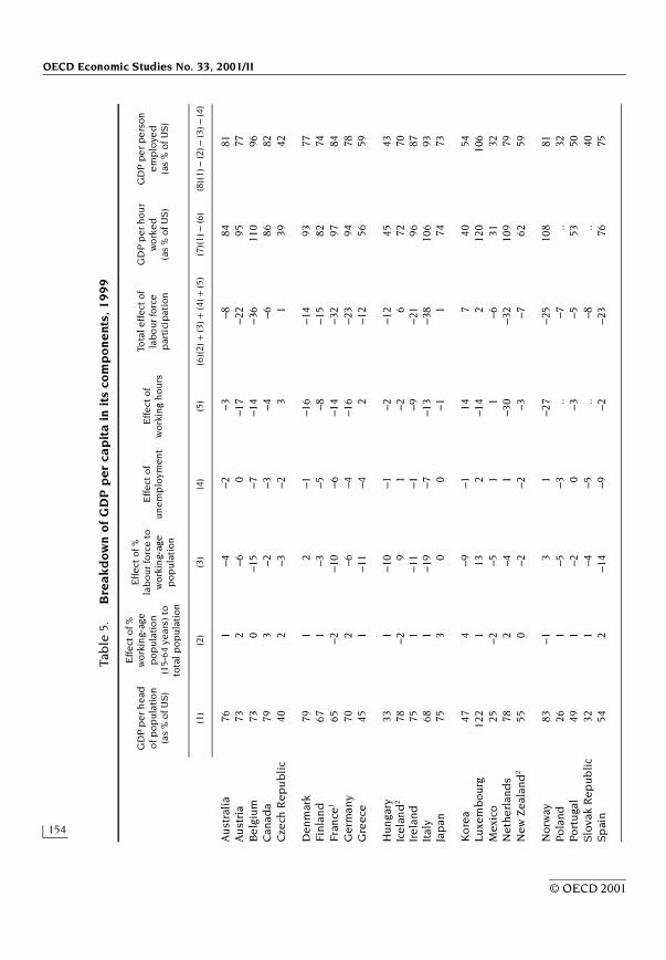
OECD Economic Studies No. 33, 2001/II
154
© OECD 2001
Tab
le 5
. B
rea
kd
own
of
GD
P p
er c
ap
ita
in i
ts c
om
po
ne
nts,
19
99
GD
P p
er
he
ad
of p
op
ula
tio
n
(as
% o
f US
)
Eff
ect
of %
w
ork
ing-
age
p
op
ula
tio
n
(15-
64 y
ear
s) t
o
tota
l p
op
ula
tio
n
Eff
ect
of %
la
bo
ur
forc
e t
o
wo
rkin
g-ag
e
po
pu
lati
on
Eff
ect
of
un
em
plo
yme
nt
Eff
ect
of
wo
rkin
g h
ou
rs
Tota
l eff
ect
of
lab
ou
r fo
rce
p
arti
cip
atio
n
GD
P p
er
ho
ur
wo
rke
d
(as
% o
f U
S)
GD
P p
er
pe
rso
n
em
plo
yed
(a
s %
of
US
)
(1)
(2)
(3)
(4)
(5)
(6)(
2)+
(3)
+ (
4)+
(5)
(7)(
1) –
(6)
(8)(
1) –
(2)
– (
3) –
(4)
Au
stra
lia
761
–4–2
–3–8
8481
Au
stri
a73
2–6
0–1
7–2
295
77B
elg
ium
730
–15
–7–1
4–3
611
096
Can
ada
793
–2–3
–4–6
8682
Cze
ch R
epu
bli
c40
2–3
–23
139
42
Den
mar
k79
12
–1–1
6–1
493
77Fi
nlan
d67
1–3
–5–8
–15
8274
Fran
ce1
65–2
–10
–6–1
4–3
297
84G
erm
any
702
–6–4
–16
–23
9478
Gre
ece
451
–11
–42
–12
5659
Hun
gary
331
–10
–1–2
–12
4543
Icel
and
278
–29
1–2
672
70Ir
ela
nd75
1–1
1–1
–9–2
196
87It
aly
681
–19
–7–1
3–3
810
693
Jap
an75
30
0–1
174
73
Ko
rea
474
–9–1
147
4054
Luxe
mb
our
g12
21
132
–14
212
010
6M
exic
o25
–2–5
11
–631
32N
ethe
rlan
ds
782
–41
–30
–32
109
79N
ew Z
eala
nd2
550
–2–2
–3–7
6259
Nor
way
83–1
31
–27
–25
108
81Po
land
261
–5–3
..–7
..32
Port
uga
l49
1–2
0–3
–553
50Sl
ovak
Rep
ublic
321
–4–5
..–8
..40
Spai
n54
2–1
4–9
–2–2
376
75
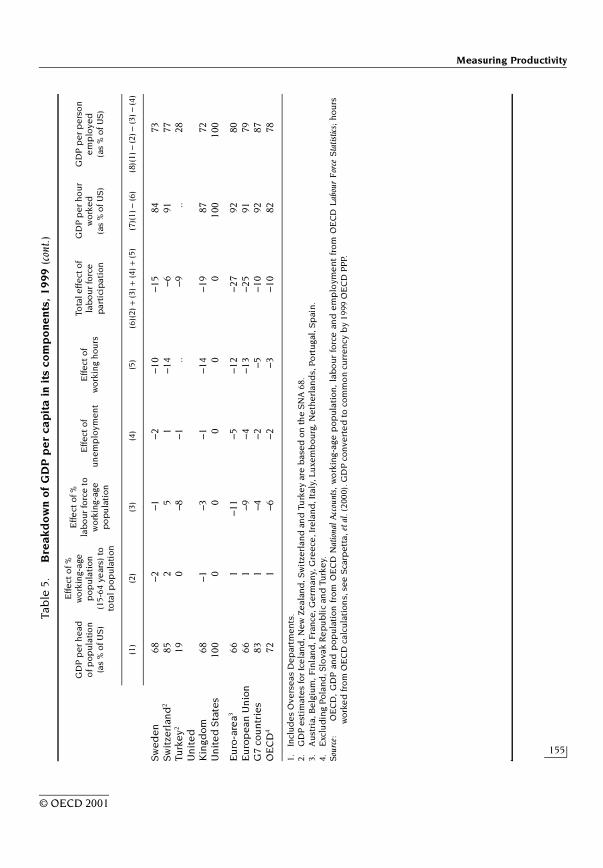
Measuring Productivity
155
© OECD 2001
Tab
le 5
. B
reak
do
wn
of
GD
P p
er
cap
ita
in
its
co
mp
one
nts
, 1
999
(co
nt.)
1.In
clu
de
s O
vers
eas
De
par
tme
nts
.2.
GD
P e
stim
ate
s fo
r Ic
ela
nd
, Ne
w Z
eal
and
, Sw
itze
rlan
d a
nd
Tu
rke
y ar
e b
ase
d o
n t
he
SN
A68
.3.
Au
stri
a, B
elg
ium
, Fin
lan
d, F
ran
ce, G
erm
any,
Gre
ece
, Ire
lan
d, I
taly
, Lu
xem
bo
urg
, Ne
the
rlan
ds,
Po
rtu
gal,
Sp
ain
.4.
Exc
lud
ing
Po
lan
d, S
lova
k R
ep
ub
lic
and
Tu
rke
y.S
ourc
e:
OE
CD
, G
DP
an
d p
op
ula
tio
n f
rom
OE
CD
Nat
iona
l A
ccou
nts,
wo
rkin
g-ag
e p
op
ula
tio
n,
lab
ou
r fo
rce
an
d e
mp
loym
en
t fr
om
OE
CD
Lab
our
For
ce S
tatis
tics;
ho
urs
wo
rke
d f
rom
OE
CD
cal
cula
tio
ns,
se
e S
carp
ett
a, e
tal.
(200
0). G
DP
co
nve
rte
d t
o c
om
mo
n c
urr
en
cy b
y 19
99 O
EC
D P
PP.
GD
P p
er
he
ad
of p
op
ula
tio
n
(as
% o
f US
)
Eff
ect
of %
w
ork
ing-
age
p
op
ula
tio
n
(15-
64 y
ear
s) t
o
tota
l po
pu
lati
on
Eff
ect
of %
la
bo
ur
forc
e t
o
wo
rkin
g-ag
e
po
pu
lati
on
Eff
ect
of
un
em
plo
yme
nt
Eff
ect
of
wo
rkin
g h
ou
rs
Tota
l eff
ect
of
lab
ou
r fo
rce
p
arti
cip
atio
n
GD
P p
er
ho
ur
wo
rke
d
(as
% o
f U
S)
GD
P p
er
pe
rso
n
em
plo
yed
(a
s %
of
US
)
(1)
(2)
(3)
(4)
(5)
(6)(
2)+
(3)
+ (
4)+
(5)
(7)(
1) –
(6)
(8)(
1) –
(2)
– (
3) –
(4)
Swed
en68
–2–1
–2–1
0–1
584
73Sw
itze
rlan
d2
852
51
–14
–691
77Tu
rkey
219
0–8
–1..
–9..
28U
nit
ed
K
ingd
om68
–1–3
–1–1
4–1
987
72U
nit
ed
Sta
tes
100
00
00
010
010
0
Eu
ro-a
rea3
661
–11
–5–1
2–2
792
80E
uro
pea
n U
nio
n66
1–9
–4–1
3–2
591
79G
7 co
unt
ries
831
–4–2
–5–1
092
87O
EC
D4
721
–6–2
–3–1
082
78
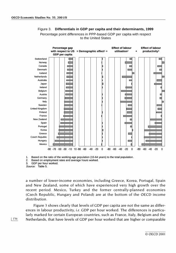
OECD Economic Studies No. 33, 2001/II
156
© OECD 2001
a number of lower-income economies, including Greece, Korea, Portugal, Spainand New Zealand, some of which have experienced very high growth over therecent period. Mexico, Turkey and the former centrally-planned economies(Czech Republic, Hungary and Poland) are at the bottom of the OECD incomedistribution.
Figure 3 shows clearly that levels of GDP per capita are not the same as differ-ences in labour productivity, i.e. GDP per hour worked. The differences is particu-larly marked for certain European countries, such as France, Italy, Belgium and theNetherlands, that have levels of GDP per hour worked that are higher or comparable
Figure 3. Differentials in GDP per capita and their determinants, 1999Percentage point differences in PPP-based GDP per capita with respect
to the United States
-90 -70 -50 -30 -10 10 -80 -80 -80-60 -40 -20 0 -60 -40 -20 0 -60 -40 -20 0
Percentage gapwith respect to US
GDP per capitaDemographic effect1
Effect of labourutilisation2
Effect of labourproductivity3++=
Switzerland
Norway
Canada
Denmark
Iceland
Netherlands
Australia
Japan
Belgium
Austria
Germany
Ireland
Italy
Sweden
United Kingdom
Finland
France
New Zealand
Spain
Portugal
Korea
Greece
Czech Republic
Hungary
Mexico
1. Based on the ratio of the working-age population (15-64 years) to the total population.2. Based on employment rates and average hours worked.3. GDP per hour worked.Source: Table 5.
Measuring Productivity
157
© OECD 2001
to the United States but much lower levels of GDP per capita. Low labour utilisation,i.e. low employment rates and short working hours, explains the bulk of this gap. Formost other OECD countries, in particular those at the bottom end of the OECD incomedistribution, labour productivity is closely linked to levels of GDP per capita.
High labour productivity is often associated with strong economic perfor-mance. However, some countries, with high levels of labour productivity have verylow levels of labour utilisation, suggesting that high labour productivity may partlybe due to increasing the capital-labour ratio and to pushing low-productivity work-ers into unemployment or out of the labour force. Estimates of GDP per hourworked should therefore ideally be looked at in combination with estimates ofGDP per capita.
THE INTERPRETATION OF PRODUCTIVITY MEASURES
Productivity is an important yardstick of economic performance. Differentproductivity measures are, however, often used without sufficient clarity about thespecific measure that is being used and its correct interpretation. This sectionbriefly touches on six of the most common uses made of productivity measuresand possible pitfalls: the relationship between productivity growth and technolog-ical change; the link between productivity and costs; productivity over the busi-ness cycle; the difference between productivity and efficiency; the links betweenindustry and firm-level productivity growth; and innovation and productivitygrowth.
The link with technological change
Multi-factor productivity growth is often interpreted as an indicator of techno-logical progress. This is not entirely correct for three reasons: i) technologicalchange does not necessarily translate into MFP growth; ii) MFP growth is not nec-essarily caused by technological change; and iii) MFP may understate the eventualimportance of productivity change in stimulating the growth of output. Thesethree factors are discussed below.
Some technological change does not translate into MFP growth becauseembodied technological change, such as advances in the quality of new vintagesof capital or improved human capital, is reflected instead in the measured contri-butions of capital and labour to output growth. Disembodied technical change, onthe other hand, will be reflected in MFP growth as it relates to advances in scien-tific knowledge, and to the diffusion of knowledge on how things are done, includ-ing better management and organisational change. MFP should also include the
OECD Economic Studies No. 33, 2001/II
158
© OECD 2001
spill-over effects from capital and labour, e.g. network effects arising from invest-ment in information technology products.
Conceptually, and following Jorgenson (1995a), the MFP term reflects all thoseeffects on output growth that are not investment, where investment is understoodas the commitment of current resources in the expectation of future returns,implying that these returns can be internalised by the investor. The distinction isimportant because the diffusion of embodied technical change is dependent onmarket transactions: investment in the improved capital or intermediate good willbe undertaken until its marginal contribution to revenue generation just equals itsuser cost, itself dependent on the market price of the capital good. The diffusionof disembodied technical change is not necessarily associated with market trans-actions. Information may circulate freely and its use by one person does not nor-mally restrict its use by another one.
When the measure for the quantity of capital services used in the MFP calcu-lation is based on a price index that reflects quality changes in capital goods,embodied technological change is captured by the growth contribution of capitaland not by the residual MFP. Conversely, when the capital goods price index is notadjusted for quality change, both embodied and disembodied technologicalchange will be picked up by the MFP residual. As Hulten (1992) showed, theembodiment part of technology can be measured by comparing capital inputbased on quality-adjusted price indices and capital input based on unadjustedprice indices. This idea was also pursued by Greenwood et al. (1997) and Bassaniniet al. (2000).
Data and resource constraints often do not permit a careful differentiationand full coverage of all labour and capital inputs. As a consequence, some of theembodiment effects of technological change and some or all of the changes in theskill composition of labour input are picked up by the MFP residual. Thus, the cor-rect interpretation of the productivity term with respect to technological changerequires knowledge about the methodology used to compute time series of capi-tal and labour input.
Just as some technological change does not correspond to MFP growth, someMFP growth is not caused by technological change. Even where the residualreflects part or all of technological change, several other factors will also bear onmeasured MFP. Such factors include adjustment costs, economies of scale, cyclicaleffects, inefficiencies and measurement errors. This is confirmed by econometricstudies that link MFP growth to technology variables, in particular research anddevelopment and patents or those that explicitly control for adjustment costs orallow for non-constant returns to scale. Research and development expenditure,for example, tends to show a statistically significant relation to productivitygrowth, but only explains a relatively small part of the overall annual movements
Measuring Productivity
159
© OECD 2001
in MFP.20 This indicates the presence of other factors. Measures of MFP are thusbetter interpreted as measures of improvements in overall efficiency than as pureexpressions of technical change.
Finally, MFP may understate the eventual importance of productivity changein stimulating the growth of output. This reflects the fact that in growth accountingmodels, capital is considered an exogenous input to the production process. In adynamic context, this is no longer the case and a feedback mechanism existsbetween productivity change and capital. Suppose that technical change allowsmore output to be produced per person. The static MFP residual measures justthis effect of technical change. Typically, however, additional output per personwill lead to additional savings and investment, and to a rise in the capital-labourratio. A traditional growth accounting framework would identify this induced effectas a growth contribution of capital, although it can be traced back to an initial shiftin technology. Thus, the MFP residual correctly measures the shift in productionpossibilities but does not capture the induced effects of technology on growth(Rymes, 1971; Hulten, 2000).
Productivity growth and changes in costs
Productivity measures are typically derived on the basis of production func-tions and quantity measures of inputs and outputs. Under certain conditions(e.g. cost minimisation), an equivalent and intuitively appealing “dual” approachexists that expresses advances in productivity as downward shifts of a cost func-tion. A cost function shows the minimum input cost of producing a certain level ofoutput, given a set of input prices. Thus, the MFP productivity residual can bemeasured either in the residual growth of output not explained by the growth ofinputs, or as the residual decline in average costs not explained by changes ininput prices. A slightly different formulation is that productivity growth equals thediminution of total costs that is explained neither by a fall in output nor by substi-tution of inputs that have become relatively more expensive for those whose rela-tive price has fallen.
The formulation of MFP in terms of average costs demonstrates once morethat productivity is not necessarily technological change and that technologicaladvances do not necessarily translate into a change of the MFP residual. It is intu-itively plausible that total and average costs can be reduced by factors other thantechnological change, such as organisational innovations or learning by doing(Harberger, 1998). The cost approach also shows how embodied technologicalchange can reduce the costs of inputs and trigger substitution processes without,however, changing the rate of multi-factor productivity growth.
OECD Economic Studies No. 33, 2001/II
160
© OECD 2001
The role of the business cycle in productivity growth
Most productivity measures are pro-cyclical, accelerating during periods ofeconomic expansion and decelerating during periods of recession. In part, this isdue to inadequate measurement. While cyclical variations in volume output tendto be measured quite accurately in economic statistics, variations in the rate ofutilisation of inputs are not picked up as fully. In particular, changes in the rate ofutilisation of capital equipment (i.e. changes in machine hours) are rarely capturedin these measures. Labour input, if measured by hours actually worked, betterreflects the changing rate of utilisation of manpower, but remains an imperfectmeasure. Consequently, increases in the rate of capacity utilisation in periods ofexpansion will cause output measures to show more rapid growth, but input mea-sures may remain stable or grow less rapidly. The result is a rise in measured pro-ductivity growth. The converse holds for periods of recession.
Even if capacity utilisation were accurately measured, difficulties wouldremain in reconciling the standard productivity model with the realities of thebusiness cycle. Much of the economic and index number theory used to guide theconstruction of these measures relies on long-term, equilibrium relationships.Since little or no account is taken of unforeseen events or disequilibria, the eco-nomic model of productivity measurement is more appropriately applied to peri-ods of continued and moderate expansion, than to rapidly changing phases of thebusiness cycle. This limitation means that year-to-year changes in productivitygrowth should not be interpreted prima facie as shifts in disembodied technology.For this purpose it is preferable to examine productivity growth patterns overlonger periods of time or adjust productivity estimates for cyclical fluctuations.21
Moreover, it is wise not to draw strong conclusions about shifts in productivityfrom the evidence of just a few years.
The difference between productivity and efficiency
Productivity and efficiency are related, but not identical concepts (Sharpe,1995). A firm or industry is considered to be inefficient if it could produce moreoutput with existing inputs, i.e. the firm is not on the production possibility curve,but within it. Productivity relates the quantity of output produced to one or moreinputs used in its production, irrespective of the efficiency of their use. In analys-ing productivity growth across countries, the difference between these two con-cepts allows a distinction between three different processes. First, productivitygrowth can result from innovative activity that results in an outward shift of the glo-bal production possibility frontier. Second, firms can improve productivity byadopting production processes and products developed elsewhere (imitation).Diffusion differs conceptually from efficiency gains, as the latter relates toimprovements made in using a given technology – even when this technology is
Measuring Productivity
161
© OECD 2001
outdated by international standards. Third, productivity growth may also be dueto reduced (technical) inefficiency. An inefficient firm or industry uses moreresources and factor inputs than required by a particular technology, thus tyingresources to low-productivity activities and reducing the overall allocative effi-ciency of an economy. Understanding the reasons behind productivity growth istherefore necessary before attributing such changes to specific sources.
How productivity at the industry level is related to that at the firm level
The main focus of this paper has been productivity measurement at theindustry and aggregate level of the economy. Industries and branches are them-selves made up of individual firms and establishments and new micro-level data-bases have greatly enhanced the possibilities for empirical research to better howunderstand individual units’ productivity performance carries over to what isobserved at the industry level. Several important conclusions have arisen from asignificant body of studies (Haltiwanger, 2000; Bartelsman and Doms, 2000; OECD,2001b). First, there are large differences in productivity performance between indi-vidual units. Second, there is a continuous and large-scale re-allocation of outputsand inputs between producers, including within industries. Third, this re-allocationcontributes significantly to aggregate productivity growth. For example, Haltiwangerreports that for the United States manufacturing sector, roughly half of multi-factorproductivity growth over the course of a recent decade can be accounted for bythe re-allocation of outputs and inputs away from less productive to more produc-tive businesses.
These findings do not invalidate the theory of productivity measurement inthis paper that essentially treats an industry, a sector or even the entire economyas if it were a single firm. Rather, it adds to the understanding and interpretationof measured productivity growth. For example, it points to one mechanism bywhich an industry as a whole implements technical change: if new technology ismainly adopted by new establishments, productivity growth occurs with entry andexit, and this requires re-allocation. Technical advances at the industry level arethen associated with the diffusion of new technology among establishments,rather than with a simultaneous shift in the production frontier of an existing set ofbusinesses. This provides an additional interpretation of changes in the produc-tivity residual at the industry level. Micro-level data studies with their focus onfirm dynamics, entry and exit and re-allocation of resources also form a natural linkto the question how innovation and “creative destruction” (see below) translateinto industry-level productivity growth. Nonetheless, micro-level approaches can-not replace the more aggregate type of productivity measurement. This is due topoor data quality at the firm or establishment level (e.g. for capital input) and thetimeliness and exhaustiveness of the available data sets. But micro-level studies
OECD Economic Studies No. 33, 2001/II
162
© OECD 2001
enhance our understanding of the underlying drivers and dynamics of productivitygrowth.
Innovation and productivity
Most approaches to measuring productivity are firmly rooted in a neo-classicalequilibrium concept. Equilibrium conditions are very important because theyhelp to guide measurement of parameters that would otherwise be difficult toidentify. Although its usefulness is generally recognised, it has been argued thatan equilibrium approach sits uneasily with the notion of innovation and produc-tivity growth. Evolutionary economists (e.g. Dosi, 1988; Nelson and Winter, 1982;Nelson, 1981) argue that innovation and technical change occur as a conse-quence of information asymmetries, and market imperfections. In a quite funda-mental sense, innovations and information asymmetries are one and the samephenomenon. Indeed, such asymmetries can scarcely be termed market imper-fections when they are necessary conditions for any technical change to occur ina market economy (Metcalfe, 1996). The point made by evolutionary economistsis that equilibrium concepts may be the wrong tools to approach the measure-ment of productivity change, because if there truly was equilibrium, there wouldbe no incentive to search, research and to innovate, and there would be no pro-ductivity growth.
Such criticism has to be taken seriously in the interpretation and use of pro-ductivity measures. An important lesson from this debate is that accounting is notexplaining the underlying causes of growth. Griliches (1997) makes a related point:
“We can take productivity growth calculation and allocate it in great detail to the variousmissed components, reducing thereby the role of the “unallocated” residual. But this, whilevery instructive and valuable, only shifts the problem to a new set of questions: why wasthere all this investment in human capital? Will it continue? Where did the improvements incapital equipment come from? […] Real explanations will come from understanding thesources of scientific and technological advances and from identifying the incentives and cir-cumstances that brought them about and that facilitated their implementation and diffusion.Explanation must come from comprehending the historical detail.”
This does not invalidate the usefulness of the standard equilibrium approachto productivity measurement, discussed in this paper, but alerts us to some of itslimits. What emerges is the complementarity of approaches: growth accountingand productivity measurement allow the systematic and consistent quantificationof the proximate sources of growth. It has explanatory power in that it captures theworkings of supply of, demand for and substitution between categories of measur-able inputs. At the same time, growth accounting has to be complemented by
Measuring Productivity
163
© OECD 2001
institutional, historical and case studies if one wants to explore the underlyingcauses of growth, innovation and productivity change.
IN CONCLUSION
The measurement of productivity continues to generate substantial interestin many countries, since productivity is a key yardstick of economic performance.This paper has discussed the main measurement difficulties that need to be con-fronted when calculating productivity indicators and has provided guidance toresearchers and statisticians in addressing these difficulties. Substantial progresshas been made in recent years to improve the comparability of productivity statis-tics. In many countries, however, basic source data are still the key limitation tothe development of comparable indicators of productivity. In addition, statisti-cians, researchers and policy makers need to be more aware of the way in whichproductivity statistics are used and their appropriate interpretation.
OECD Economic Studies No. 33, 2001/II
164
© OECD 2001
NOTES
1. Multi-factor productivity is sometimes referred to as total factor productivity. Multi-factor productivity implies that several factors are included as inputs, though not nec-essarily all. Total factor productivity suggests that all possible factors are included. Inpractice, this is seldom the case.
2. This definition is consistent with the System of National Accounts 1993.
3. Recently, Nordhaus (2001) discussed the link between industry-level and aggregateproductivity measures based on value added. He presented alternative methods formeasuring productivity growth that are derived from the link between productivityand welfare. Nordhaus showed that, under a number of restrictive assumptions, awelfare-related productivity measure can be constructed as a weighted average ofproductivity growth in individual industries. One specific conclusion is that macroeco-nomic productivity gains that arise from shifts between industries with different pro-ductivity levels should be excluded from welfare-oriented productivity measures.
4. This is a general form of double-deflation, expressed in a continuous-time Divisiaindex.
5. To interpret value-added-based MFP growth as a measure of disembodied technicalchange, one has to assume that technical change operates only on primary inputs, andnot on intermediate ones. There is little empirical evidence to support this assumption.
6. For a discussion regarding the United States, see Eldridge (1999).
7. See the OECD Handbook on the Quality Adjustment of Price Indices for ICT Products (forthcoming)and the Eurostat Handbook on Price and Volume Measures in National Accounts (forthcoming).
8. For an overview, see Bresnahan and Gordon (1996).
9. For example, Lowe (1996) provides an overview of how quality change is handled inthe Canadian National Accounts.
10. For empirical results see United States Bureau of Labor Statistics (1993), Fosgerau et al.(2001) and Scarpetta et al. (2000).
11. For specific information about the practical and conceptual issues regarding the con-struction of capital stock measures, see the OECD Manual on Capital Measurement (2001).
12. Van Ark (1996) and Pilat (1997) discuss these issues in greater detail. See alsoO’Mahony (1999).
13. Estimates of quality-adjusted labour input are available for some countries, see forexample O’Mahony (1999).
14. Levels of capital productivity and multi-factor productivity for five major OECD econo-mies (United States, Japan, Germany, France, United Kingdom) are estimated inO’Mahony (1999).

Measuring Productivity
165
© OECD 2001
15. An additional problem concerns the deflators that are used to measure investment.See Colecchia and Schreyer (2001).
16. Ongoing work on the OECD Capital Stock Manual and the OECD Productivity Manual mayhelp in enhancing the comparability of capital stock estimates across countries.
17. The Internet site of the OECD Statistics Department provides an overview of some ofthe key issues related to the construction of purchasing power parities, seewww.oecd.org/std/ppps.htm. An evaluation of the PPP programme was prepared by theformer chief statistician of the Australian Bureau of Statistics, Ian Castles, in 1997(OECD, 1997), and has led to a range of improvements in the construction of PPPs. Therecent benchmark study for 1996 also contains an extensive discussion of many of theissues related to the OECD/Eurostat work on PPPs (OECD, 1999b).
18. See Elteto and Koves (1964); Szulc (1964); Geary (1958); and Khamis (1970). Moreelaborate descriptions of these methods and the differences between them are avail-able in OECD (1999b). See also Van Ark (1996), Pilat (1997) and OECD (1998) for a dis-cussion of the use of PPPs for international comparisons of productivity.
19. The EKS method is closely related to superlative index numbers, such as theTheil-Tornqvist index.
20. See the paper by Guellec and Van Pottelsberghe in this issue of OECD Economic Studies.
21. More detail on the trend-adjustment of productivity growth is available in Scarpettaet al. (2000).
OECD Economic Studies No. 33, 2001/II
166
© OECD 2001
BIBLIOGRAPHY
ARK, B. VAN (1996),“Issues in Measurement and International Comparison of Productivity – An Overview”,in OECD (1996), Industry Productivity – International Comparison and Measurement Issues, Paris,pp. 19-47.
ARK, B. VAN and R.H. McGUCKIN (1999),“International comparisons of labor productivity and per capita income”, Monthly LaborReview, July 1999, pp. 33-41.
BALK, B. (1995),“Axiomatic price index theory: A survey”, International Statistical Review 63, pp. 69-93.
BARRO, R.J. and X. SALA-i-MARTIN (1995),Economic Growth, MIT Press.
BARTELSMAN, E. and M. DOMS (2000),“Understanding productivity: lessons from longitudinal microdata”, Journal of EconomicLiterature 38(3), September, pp. 569-94.
BASSANINI, A., S. SCARPETTA and I. VISCO (2000),“Knowledge, technology and economic growth: recent evidence from OECD countries”,OECD Economics Department Working Papers No. 259.
BRESNAHAN, T.F. and R.J. GORDON (eds.) (1996),The Economics of New Goods, Studies in Income and Wealth, University of Chicago Press.
BUREAU OF LABOR STATISTICS (1993),Labor Composition and U.S. Productivity Growth, 1948-90, US Government Printing Office.
COLECCHIA, A. and P. SCHREYER (2001),“The impact of information and communications technologies on output growth”, STIWorking Paper 2001/07, OECD, Paris.
DEAN, E.R., M.J. HARPER and M.S. SHERWOOD (1996),“Productivity measurement with changing-weight indices of outputs and inputs”, inOECD (1996a), Industry Productivity – International Comparison and Measurement Issues, pp. 183-215.
DENISON, E.F. (1985),Trends in American Economic Growth 1929-82, Brookings Institution, Washington, D.C.
DIEWERT, W.E. (1976),“Exact and superlative index numbers”, Journal of Econometrics, pp. 115-45.
DOSI, G. (1988),“Sources, procedures and micro-economic effects of innovation”, Journal of EconomicLiterature 36.

Measuring Productivity
167
© OECD 2001
ENGLANDER, S. and A. GURNEY (1994),“Medium-term determinants of OECD productivity”, OECD Economic Studies, No. 22,Spring, pp. 49-109.
ELDRIDGE, L.P. (1999),“How price indexes affect productivity measures”, Monthly Labor Review, February,pp. 35-46.
ELTETO, O. and P. KOVES (1964),“On an index computation problem in international comparisons” (in Hungarian),Statistztikai Szemle, Vol. 42, pp. 507-518.
FISHER, I. (1922),The Making of Index Numbers, Boston.
FOSGERAU, M., S.E. HOUGAARD JENSEN and A. SØRENSEN (2001),“Measuring educational heterogeneity and labour quality: A note”, CEBR Discussionpaper 2001-6, www.cebr.dk.
GEARY (1958),“A note on comparisons of exchange rates and purchasing power between countries”,Journal of the Royal Statistical Society, Vol. 121, 97-99, pt. 1.
GREENWOOD, J., Z. HERCOWITZ, and P. KRUSELL (1997),“Long-run implications of investment-specific technological change”, American EconomicReview Vol. 87(3), pp. 342-62.
GRILICHES, Z. (1997),“R&D and the productivity slowdown: is recovery around the corner?”, unpublishedmimeo.
HALTIWANGER, J. (2000),“Aggregate growth: what have we learned from microeconomic evidence?”, OECD Eco-nomics Department Working Papers, No. 276, OECD, Paris.
HARBERGER, A.C. (1998),“A vision of the growth process”, American Economic Review, March, pp. 1-32.
HILL, P. (1999a),“The productive capital stock and the quantity index for flows of capital services”;paper presented at the third meeting of the Canberra Group on Capital Stock Statistics,Washington, D.C.
HULTEN, C. (1992),“Growth accounting when technical change is embodied in capital”, American EconomicReview, Vol. 82 (4), pp. 964-80.
HULTEN, C. (2001),“Total factor productivity: A short biography”, in: Hulten, Dean and Harper (eds.). NewDevelopments in Productivity Analysis, University of Chicago Press for the National Bureau ofEconomic Research
JORGENSON, D. (1963),“Capital theory and investment behaviour”, American Economic Review, Vol. 53, pp. 247-259.
JORGENSON, D. (1995a),Productivity Volume 1: Postwar US Economic Growth, MIT Press.
JORGENSON, D. (1995b),Productivity Volume 2: International Comparisons of Economic Growth, MIT Press.

OECD Economic Studies No. 33, 2001/II
168
© OECD 2001
JORGENSON, D., F. GOLLOP and B. FRAUMENI (1987),Productivity and US Economic Growth, Harvard University Press, MA.
JORGENSON, D. and Z. GRILICHES (1967),“The explanation of productivity change”, Review of Economic Studies 34.
KHAMIS, S.H. (1970),“Properties and conditions for the existence of a new type of index number”, Sankhya,Series B, Vol. 32, Parts 1 and 2.
KONÜS, A.A. (1924),“The problem of the true index of the cost of living”, translated in Econometrica (1939) 7,pp. 10-29.
KRAVIS, I.B., A. HESTON and R. SUMMERS (1982),World Product and Income, Johns Hopkins University Press, Baltimore.
KURODA, M., K. MOTOHASHI and K. SHIMPO (1996),“Issues on the international comparison of productivity: theory and measurement”, inOECD (1996a),Industry Productivity – International Comparison and Measurement Issues, Paris, pp. 49-95.
LOWE, R. (1996),“Handling quality changes in the Canadian National Accounts price deflators”, inOECD(1996a), Industry Productivity – International Comparison and Measurement Issues, pp. 143-157.
MADDISON, A. (1991),Dynamic Forces in Capitalist Development, Oxford University Press, Oxford.
MADDISON, A. (1995),Monitoring the World Economy, 1820-1992, OECD, Paris.
METCALFE, S. (1996),“The economic foundations of technology policy: equilibrium and evolutionary per-spectives”, in P. Stoneman (ed.) (1996), Handbook of the Economics of Innovation and Technolog-ical Change, pp. 409-512.
MORRISON, C.J. (1986),“Productivity measurement with non-static expectations and varying capacity utiliza-tion”, Journal of Econometrics 33.
MOULTON, B.R., R.P. PARKER and E.P. SESKIN (1999),“A preview of the 1999 comprehensive revision of the national income and productaccounts – definitional and classificational changes”, Survey of Current Business, August,pp. 7-20, Bureau of Economic Analysis.
NADIRI, I. and I. PRUCHA (2001),“Dynamic factor demand models and productivity analysis”, Hulten, Dean and Harper(eds.), New Developments in Productivity Analysis, University of Chicago Press for theNational Bureau of Economic Research.
NELSON, R. (1981),“Research on productivity growth and productivity differences: dead ends and newdepartures”, Journal of Economic Literature.
NELSON, R. and S. WINTER (1982),An Evolutionary Theory of Economic Change, Cambridge, Mass., Harvard University.

Measuring Productivity
169
© OECD 2001
NORDHAUS, W.D. (2001),“Alternative methods for measuring productivity growth”, NBER Working Paper 8095,National Bureau of Economic Research, Cambridge, MA.
OECD (1996a),Industry Productivity: International Comparison and Measurement Issues, OECD Proceedings,Paris.
OECD (1996b),Services: Measuring Real Value Added, Paris.
OECD (1996c),OECD Input-Output Tables, Paris.
OECD (1997),“Review of the OECD-Eurostat PPP Program”, Paris, available at www.oecd.org/std/ppp/pps.htm.
OECD (1998a),Technology, Productivity and Job Creation, Paris.
OECD (1998b),“The dynamics of industrial performance – what drives productivity growth”, OECD Sci-ence, Technology and Industry Outlook 1998, Paris.
OECD (1999a),Employment Outlook, Paris.
OECD (1999b),“Purchasing power parities and real expenditures – EKS Results, 1996”, Paris.
OECD (2000),“Underground, informal and illegal activities (non-observed economy): creation andcontent of a measurement handbook”, STD/NA(2000)21, OECD, Paris.
OECD (2001a),OECD Productivity Manual: A Guide to the Measurement of Industry-Level and Aggregate Productiv-ity Growth, OECD, Paris, www.oecd.org/subject/growth/prod-manual.pdf.
OECD (2001b),“Productivity and firm dynamics”, OECD Economic Outlook, No. 69, Paris, June.
O’MAHONY (1999),Britain’s Productivity Performance 1950-1996 – An International Perspective, National Institute ofEconomic and Social Research, London.
PILAT, D. (1997),“Competition, productivity and efficiency”, OECD Economic Studies, No. 27, 1996/II,pp. 107-145, OECD, Paris.
RYMES, T.K. (1971),On Concepts of Capital and Technological Change, Cambridge.
SCARPETTA, S., A. BASSANINI, D. PILAT and P. SCHREYER (2000),“Economic growth in the OECD area: recent trends at the aggregate and sectoral level”,OECD Economics Department Working Papers, No. 248, OECD, Paris.
SCHREYER, P. (2001),“Computer price indices and international growth comparisons”, Growth Project Back-ground Papers, OECD, Paris, www.oecd.org/subject/growth/products/index.htm.

OECD Economic Studies No. 33, 2001/II
170
© OECD 2001
SHARPE, A. (1995),“International perspectives on productivity and efficiency”, Review of Income and Wealth,Vol. 41, No. 2, June, pp. 221-237.
SZULC, B. (1964),“Index numbers of multilateral regional comparisons” (in Polish), Przeglad Statysticzny,Vol. 3, pp. 239-254.