Blood Flow in Channel Constrictions: A Lattice-Boltzmann ...

Journal of Applied Fluid Mechanics, Vol. 12, No. 4, pp. 1333-1345, 2019.

Available online at www.jafmonline.net, ISSN 1735-3572, EISSN 1735-3645. DOI: 10.29252/jafm.12.04.29434

Blood Flow in Channel Constrictions: A Lattice-Boltzmann

Consistent Comparison between Newtonian and

Non-Newtonian Models

G. A. Orozco1†, C. T. Gonzalez-Hidalgo2, A. D. Mackie3, J. C. Diaz4 and D. A. Roa

Romero1

1 Faculty of Sciences, Physics Department, Universidad Antonio Nariño, Carrera 3 Este No 47 A–15, 110231

Bogotá, Colombia 2 Industrial Engineering Department, Pontificia Universidad Javeriana, Carrera 7 No 40–62, 110231

Bogotá, Colombia 3 Chemical Engineering Department, ETSEQ, Universitat Rovira i Virgili, Av. dels Països Catalans 26, 43007

Tarragona, Spain 4 GTM, Department of Planning, Carrera 46 No 91-71. 110211 Bogotá, Colombia

†Corresponding Author Email: [email protected]

(Received July 18, 2018; accepted November 25, 2018)

ABSTRACT

Lattice Boltzmann simulations have been carried out in order to study the flow of blood in normal and

constricted blood channels using Newtonian and non-Newtonian rheological models. Instead of using

parameters from previous works as is usually done, we propose a new optimization methodology that provides

in a consistent manner the complete set of parameters for the studied models, namely Newtonian, Carreau-

Yassuda and Kuang-Luo. The optimization was performed simultaneously using experimental data from

several sources. Physical observables such as velocity profiles, shear rate profiles and pressure fields were

evaluated. For the normal channel case, it was found that the Newtonian model predicts both the highest velocity

and shear rates profiles followed by the Carreau-Yassuda and the Kuang-Luo models. For a constricted channel,

important differences were found in the velocity profiles among the studied models. First, the Newtonian model

was observed to predict the velocity profile maximum at different channel width positions compared to the non-

Newtonian ones. Second, the obtained recirculation region was found to be longer for the Newtonian models.

Finally, concerning the constriction shape, the global velocity was found to be lower for a rectangular geometry than for a semi-circular one.

Keywords: Blood rheology; Lattice-boltzmann; Computational fluid dynamics; Non-newtonian models;

Simultaneous optimization.

NOMENCLATURE

c speed of sound

e lattice-boltzmann (LB) canonical velocity

vector

f LB distribution function

f eq LB equilibrium distribution function

p pressure

Re Reynolds number

u fluid velocity

w LB weighting factor

shear rate

ε Knudsen number

µ∞ viscosity at infinite shear rate

ν kinematic viscosity

σy yield stress

ρ density

τ LB relaxation time

1. INTRODUCTION

Blood plays several fundamental roles in human and

animal organisms. For instance, it transports oxygen

and nutrients to the tissues, carries the metabolism

products, protects the body from infections,

participates actively in the hemostatic process,

among many others. From a physical point of view

http://www.jafmonline.net/

G. A. Orozco et al. / JAFM, Vol. 12, No. 4, pp. 1333-1345, 2019.

1334

blood can be characterized through certain

hemodynamic variables such as apparent viscosity,

shear stress, shear rate as well as its fluid behavior

through arteries, veins or vessels. Indeed, changes in

these variables can produce alterations of the flow

pattern, the way the blood components are delivered

to an injured site and the flow conditions near the

vessel wall. (Hathcock, 2006) Additionally, if the

shear forces are not strong enough, blood viscosity

can be increased due to the aggregation of

erythrocytes and platelets. (Baskurt and Meisleman,

2003) All these phenomena might be associated with

certain types of vascular diseases.

The flow behavior of blood has been studied both

experimentally and computationally. For the first

case, some works have reported experimental

velocity profiles of blood flowing in a live vessel by

way of techniques based on fluorescent markers or

fluid nanoparticles. Such markers are inserted into

the veins of live specimens such as rats or rabbits.

The velocity distribution of blood can be obtained by

recording several images and then by reconstructing

the marker time trajectories.(Tangelder, Slaaf,

Muijtjens, Arts, and Reneman, 1986; Ha, 2012)

Another approach consists in studying the blood flow

using computational algorithms through the Navier-

Stokes equations (NSE) and assuming a rheological

model. There are several different available

methodologies that allow to numerically study the

NSE. One of them, based on the transport Boltzmann

equation, is the Lattice-Boltzmann (LB) method.

(Succi, 2001) LB is an explicit method in which the

dynamics of a fluid is modeled using a set of

interacting particles located in a discretized space

and with a set of associated probability distribution

functions that allows us to recover the macroscopic

variables such as density, momentum and energy.

Besides the LB method, other blood flow studies

have been performed using more classical

approaches such as finite elements, (Weller, 2008;

Weller, 2010) finite volumes (Sorensen, Burgreen,

Wagner, and Antaki, 1999a; Sorensen, Burgreen,

Wagner, and Antaki, 1999b) and finite differences.

(Fogelson and Guy, 2004; Anand, Rajagopal and

Rajagopal, 2005; Lobanov and Staroszhilova, 2005)

Some attempts towards including explicitly the red

blood cells have also been proposed using, for

instance, smoothed particle dynamics, (Wootton,

Popel, and Alevriadou, 2002) multiscale simulations,

(Xu, Chen, M., Rosen, and Alber, 2008) mean field

theory (Pivkin and Karniadakis, 2008) and the

cellular automata approach. (Ouared and Chopard,

2005)

From a rheological point of view, blood viscosity

presents interesting features such as shear thinning

where viscosity can drastically change from an

almost constant value at high shear rates to a

significantly higher value at low ones. During a

cardiac cycle the shear rate can change from 0 to

1000 s−1, (Cho and Kensey, 1991) and so viscosity

variations should be accounted for by using a

constitutive equation. Different works have focused

on studying the flow of blood using different models.

For instance, Ashrafizaadeh and Bakhshaei (2009)

studied the flow of blood using two dimensional LB

simulations and three non-Newtonian rheological

models obtaining velocity profiles deviations

between the Newtonian and non-Newtonian models.

Boyd et al. (2007). studied the flow of blood in

steady and oscillatory flows using two different non-

Newtonian models. (Boyd, Buick, and Green, 2007)

They found that the largest deviation from a

Newtonian behavior is given by the Casson model.

Bodnár et al. performed numerical simulations to

compare the shear-thinning and the viscoelastic

behavior of blood as a function of the flow rate, using

the Carreau-Yasuda and Oldroyd-B models. They

found that the shear-thinning effects are more

pronounced than the viscoelastic ones. (Bodnár,

Sequeira, and Prosi, 2011) Sorensen et al. (1999a)

considered platelet deposition and thrombus

formation over a collagen surface assuming a

Newtonian fluid and neglecting the effect of an

obstacle on the flow field. (Sorensen, Burgreen,

Wagner, and Antaki, 1999a) Other studies have

found relationships between the blood cell

concentration (hematocrit), the wall shear rate, and

the wall shear stress. (Box, van der Geest, Rutten,

and Reiber, 2005)

Despite the fact that the Casson model has been

widely studied, there is no agreement with respect to

its range of validity. While some studies (Milnor,

1982) state that it is only valid at shear rates ≤ 10s−1

other studies (Bate, 1977) have reported ranges

between 15 to 6400 s−1 or hematocrit concentrations

≤ 40%. (Wang, 2011) Indeed, as will be shown in

section 3.2, the Casson model does not provide a

satisfactory fit of the experimental data when the

whole range of shear rates is considered.

As mentioned above, previous works have studied

the flow behavior of blood using different

rheological models. For instance, Ashrafizaadeh et

al. compared the C-Y, K-L and Casson models using

experimental measurements of a thiocyanate

solution (blood-mimicking fluid) for the C-Y model

(Gijsen, van de Vosse, and Jansenn, 1999; Gijsen,

Allanic, van de Vosse, and Jansenn, 1999) and

human blood for the K-L and Casson models (Luo

and Kuang, 1992) This comparison is in principle not

consistent because of the different nature of the data.

On the other hand, Boyd et al. (2007) made

comparisons between the Casson and the C-Y

models performing independent fits on the same

sample. Nevertheless, we consider this procedure to

be also flawed, since the viscosity at infinite shear

rate is a parameter that couples all model equations.

Such a coupling is clearly unaccounted for when fits

are performed independently. Consequently, these

procedures might not provide reliable conclusions

and thus, for the sake of a consistent comparison, we

propose to determine the parameters for all models

using a simultaneous fit given a unique set of

experimental data. To our knowledge, this issue has

not yet been considered and therefore deserves a

detailed study.

In this work several features will be addressed,

namely: i) a new set of parameters are needed for the

Carreau-Yassuda (C-Y) and the Kuang-Luo (K-L)

models. To do so, a simultaneous fit for the two

models is performed using the same set of


1335

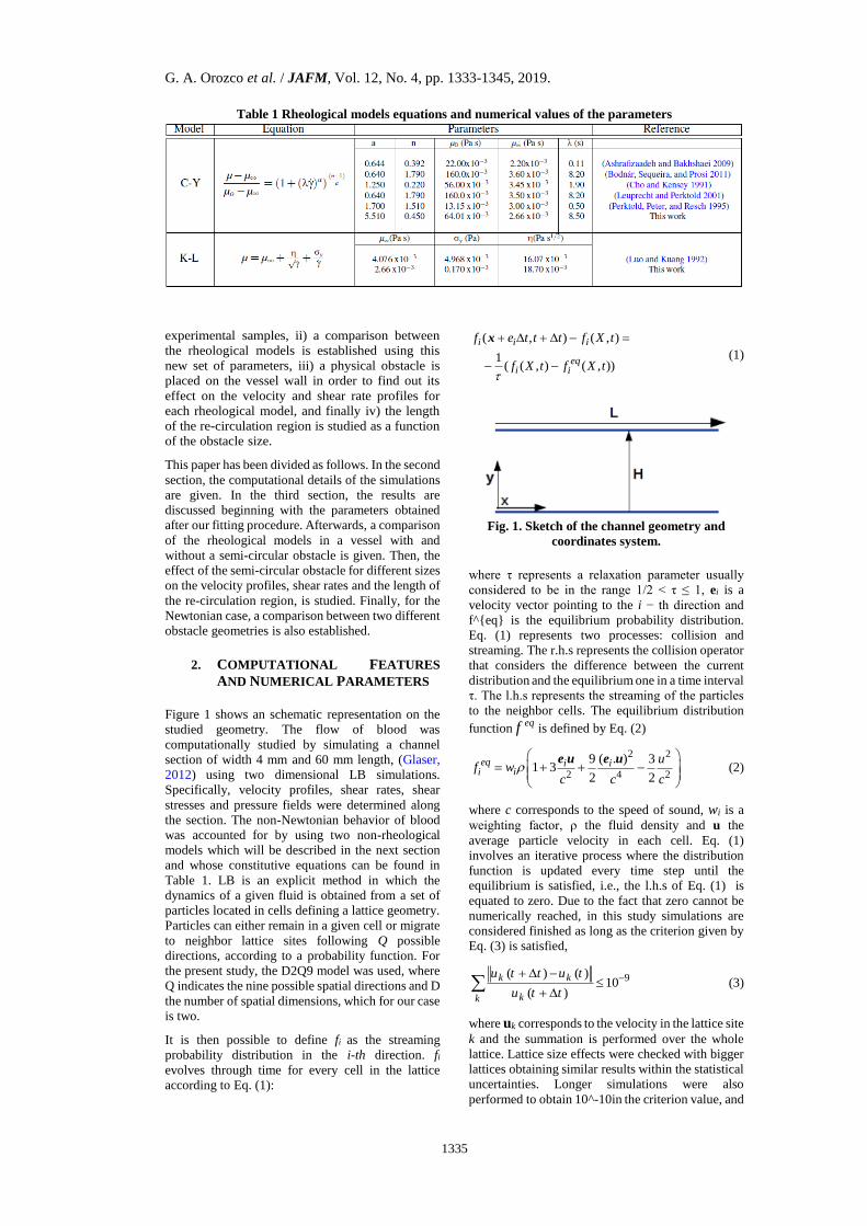
Table 1 Rheological models equations and numerical values of the parameters

experimental samples, ii) a comparison between

the rheological models is established using this

new set of parameters, iii) a physical obstacle is

placed on the vessel wall in order to find out its

effect on the velocity and shear rate profiles for

each rheological model, and finally iv) the length

of the re-circulation region is studied as a function

of the obstacle size.

This paper has been divided as follows. In the second

section, the computational details of the simulations

are given. In the third section, the results are

discussed beginning with the parameters obtained

after our fitting procedure. Afterwards, a comparison

of the rheological models in a vessel with and

without a semi-circular obstacle is given. Then, the

effect of the semi-circular obstacle for different sizes

on the velocity profiles, shear rates and the length of

the re-circulation region, is studied. Finally, for the

Newtonian case, a comparison between two different

obstacle geometries is also established.

2. COMPUTATIONAL FEATURES

AND NUMERICAL PARAMETERS

Figure 1 shows an schematic representation on the

studied geometry. The flow of blood was

computationally studied by simulating a channel

section of width 4 mm and 60 mm length, (Glaser,

2012) using two dimensional LB simulations.

Specifically, velocity profiles, shear rates, shear

stresses and pressure fields were determined along

the section. The non-Newtonian behavior of blood

was accounted for by using two non-rheological

models which will be described in the next section

and whose constitutive equations can be found in

Table 1. LB is an explicit method in which the

dynamics of a given fluid is obtained from a set of

particles located in cells defining a lattice geometry.

Particles can either remain in a given cell or migrate

to neighbor lattice sites following Q possible

directions, according to a probability function. For

the present study, the D2Q9 model was used, where

Q indicates the nine possible spatial directions and D

the number of spatial dimensions, which for our case

is two.

It is then possible to define fi as the streaming

probability distribution in the i-th direction. fi

evolves through time for every cell in the lattice

according to Eq. (1):

( , ) ( , )

1( ( , ) ( , ))

i i i

eqi i

f e t t t f X t

f X t f X t

x

(1)

Fig. 1. Sketch of the channel geometry and

coordinates system.

where τ represents a relaxation parameter usually

considered to be in the range 1/2 < τ ≤ 1, ei is a

velocity vector pointing to the i − th direction and

f^{eq} is the equilibrium probability distribution.

Eq. (1) represents two processes: collision and

streaming. The r.h.s represents the collision operator

that considers the difference between the current

distribution and the equilibrium one in a time interval

τ. The l.h.s represents the streaming of the particles

to the neighbor cells. The equilibrium distribution

function f eq is defined by Eq. (2)

2 2

2 4 2

( . )9 31 3

2 2

eq i iii

uf w

c c c

e u e u (2)

where c corresponds to the speed of sound, wi is a

weighting factor, ρ the fluid density and u the

average particle velocity in each cell. Eq. (1)

involves an iterative process where the distribution

function is updated every time step until the

equilibrium is satisfied, i.e., the l.h.s of Eq. (1) is

equated to zero. Due to the fact that zero cannot be

numerically reached, in this study simulations are

considered finished as long as the criterion given by

Eq. (3) is satisfied,

9( ) ( )10

( )

k k

kk

u t t u t

u t t

(3)

where uk corresponds to the velocity in the lattice site

k and the summation is performed over the whole

lattice. Lattice size effects were checked with bigger

lattices obtaining similar results within the statistical

uncertainties. Longer simulations were also

performed to obtain 10^-10in the criterion value, and


1336

similar results were obtained.

Bounce back boundary conditions were used to

reproduce the channel walls that were considered to

be rigid regardless of the blood pressure. For these

conditions, the components of the incoming velocity

on the wall are propagated in the opposite direction

defining a non-slip condition. At the inlet-outlet of

the channel, pressure boundary conditions were used

as proposed by Zou and He (1997) Density and

pressure are related through2

3

cp and the

Reynolds number is defined by eq-4

2 3

236

c HRe

Lv

(4)

where H and L are the channel width and length and

ν = µ∞/ρ is the kinematic viscosity. Eq. (4) allows a

pressure gradient to be imposed once the Reynolds

number is fixed. For non-Newtonian models,

viscosity is not a constant value and so in order to

determine Re the ν value is considered as the limiting

viscosity at infinite shear rate, µ∞, which is the

coupling parameter for all the constitutive equations

and can be obtained from a simultaneous fit of the

experimental data. Based on reported values for

channels of 4 mm, (Glaser, 2012) for all simulations

a Reynolds number of 500 was chosen. According to

Eq. (4) this Reynolds number defines a pressure

difference of 1.19 × 10−3 in LB units. The relaxation

parameter τ is a function of the kinematic viscosity ν

defined by Eq. (5):

13

2v (5)

As already known, when considering a non-

Newtonian behavior, ν and τ become a function of

the shear rate ˙γ. Therefore, new constitutive models

that relate them must be used. Following Krüger et

al. γ˙ is calculated through Eq. (6) . (Krüger, Varnik,

and Raabe, 2009)

(1)3

(6)

where Π(1) is defined as(1) (1) and

(1) is a

second rank tensor related to the momentum flux at

the macroscopic level defined by Eq. (7) (1) (1)

i i ii

c c f (7)

where fi(1) refers to the second term in the expansion

of the distribution function around the equilibrium,

defined in Eq. (8) :

(0) (1) (2)2 2( )i i i if f f f O (8)

From this expression, (0) eq

i if f and the

distribution function out of equilibrium is (1)neq eq

ii i if f f f being ε the Knudsen

number. Eq. (6), along with the constitutive

equations, are needed to obtain ˙γ and to calculate ν

and τ. The obtained system of equations given by γ˙

and ν can be solved either analytically or numerically

depending on the rheological model that for this

work corresponds to the C-Y (Robertson, Sequeira,

and Owens, 2009) and the K-L (Luo and Kuang,

1992) models. In particular, the K-L model allows an

analytical solution to be found while the C-Y model

requires the solution of a non-linear system of

equations that was solved using the Newton-

Raphson method.

The momentum flux tensor (1) was used to obtain

the physical quantities for every lattice cell such as

the strain and shear rate magnitudes. Alternatively,

shear rates were also calculated through a second

order finite difference scheme over the velocity

profiles. Although locality is lost using this

methodology, comparable results can be also

obtained. However, the lattice resolution should be

modified for the majority of cases through the

parameters ∆x and ∆t.

The pressure field along the studied channel was

calculated using the LB distribution given by Eq. (9)

(Kürger, Varnik, and Raabe 2009)

2 (0)p u (9)

with Π(0) defined similarly as Π(1) in Eq. (7) .

A lattice of 200×3000 square cells was used for all

simulations, with ∆x= 2× 10−5 m and ∆t=2 × 10−6 s.

This has been tuned by comparing the theoretical

velocity profiles for non-obstacle cases with those

obtained by simulation, except for the case of the C-

Y model where there is no analytical solution.

In order to study the behavior of the blood flow

around a blood clot, an obstacle was introduced at the

bottom wall of the channel centered at ∼ 27% the

channel length (16mm). Subsequently, the obstacle

size was changed in order to establish its effect over

the different profiles. The obstacle geometry was

also considered including both semi-circular and

rectangular geometries. The obstacle cells do not

perform neither collision nor streaming steps and

bounce back boundary conditions were assumed.

Four different semicircular sizes of radius 40, 80,

120 and 160 ∆x were studied, which corresponds to

20, 40, 60 and 80% of the channel width. A

rectangular obstacle of 80 ∆x length was also

considered in order to establish possible differences

between the geometries.

Numerical simulations were performed using our

in-house code developed from scratch in the C++

language and parallelized using the OpenMP

libraries. Computing time can be significantly

affected depending on the lattice size and the

rheological model. For instance, a simulation in a

lattice of 200 × 3000 using a Newtonian model

without an obstacle takes around 60 hours using 4

intel Xeon processors at 2.5 GHz, while for a non-

Newtonian model simulations require about 20%

more time. The computing time was found to

increase by approximately three when introducing

a semi-circular obstacle of 80% the channel width.


1337

3. RESULTS

3.1 Simultaneous Optimization of the

Rheological Parameters

The use of different parameters sets can cause a bias

in the analysis when comparing more than one

rheological model. This inconsistency makes it

difficult to conclude that any difference found

between the models is due to the blood behavior.

Thus, as mentioned in the Introduction, in this work

all the parameters were fitted using the same

experimental samples. The only requirement to do so

is to include a coupled parameter between the models

which, as can be seen in Table 1, corresponds here to

the viscosity at infinite shear rate (µ∞). Note that both

the K-L and the C-Y models reproduce this value in

the high shear rate limit. To the best of our

knowledge no previous works have considered this

issue.

The optimization procedure we propose requires the

minimization of an objective function defined by Eq.

(10):

exp exp2 2

2 21

( ) ( )1est KL est CYni ii i

i i i

Fn s s

(10)

where n is the total number of experimental data used

for the fitting procedure (a total of 33 data were used

(Brooks, Goodwin, and Seaman 1970; Chien, Usami,

M., L., and Gregersen, 1966; Chien, 1970; Skalak,

Keller, and Secomb 1981)), esti corresponds to the

estimation of viscosity obtained using the

rheological models, mu_i^{exp} represents the

experimental viscosity and 2is is the associated

uncertainty of the experimental data. F is an implicit

function of jy that represents the set of

rheological parameters to be fitted which

corresponds to the C-Y and K-L models given by

0, , , ,C Yjy n a

and

, ,K Lj yy

respectively.

The idea is to minimize F with respect to every

parameter jy . Thus, from the differentiation of

eq-10, it is possible to find Eq. (11) :

(11)

exp

21

exp

2

2( )1

2( )

j

est KL est KLni i i

ji i

est CY est CYi i i

ji

F

y

n ys

ys

Since the initial values are unknown for both models,

it is necessary to make a first order Taylor expansion

of esti around the initial guess 0

jy obtaining

Eq. (12)

0 0

1

( ) ( )p est

est est ii j j i j j

jj

y y y yy

1,...,i n (12)

where 0

j j jy y y and p is the number of

parameters to be fitted that depends on the

rheological model to be used. For instance, in the C-

Y model, four parameters need to be considered,

namely λ ,n ,a ,µ∞. Derivatives k

F

y

can be

explicitly calculated from the rheological equations

given in Table 1.

Replacing Eq. (12) into Eq. (11) it is finally

obtained that

exp0

2

1 exp0

2

( ) ( )

0

( ( ) ) ( )

est KLest KL ii j ji est KL

j i

nji

est CYi est CY i

i j ji est CYj i

ji

y j yy

ys

y j yy

ys

(13)

Eq. (13) represents a square linear system of the

form A∆yj = B with 7 unknowns that represent the

parameters to be simultaneously estimated

(y1,y2,...y7). Since the minimization requires several

trials, the matrix construction and solution were

implemented in our in-house code using the lower-

upper (LU) decomposition method. The optimized

parameters obtained after an iterative procedure are

presented in Table 1.

As a first approach, independent fits of every model

can be performed keeping the coupling parameter

µ∞ as a fixed value. Nonetheless, when following

this procedure the obtained parameters are different

from the simultaneous fit. Moreover, the value of the

objective function for the total set of data is also

greater indicating that this procedure does not give

the optimal solution. The reason for these different

results is related to the fact that using such an

approach, the system degrees of freedom are

reduced. However, the parameters obtained from the

independent fits can be used as initial guesses for the

simultaneous fit.

3.2 Rheological Model Parameters

As mentioned before, we considered several

rheological models, namely, Newtonian, C-Y and K-

L. Parameters of every model were simultaneously

obtained from a fit of experimental viscosities

reported from different works. Namely, Brooks

et al. reported viscosity data using suspensions of

erythrocytes (RBC) in saline and plasma. (Brooks,

Goodwin, and Seaman 1970) Chien et al. (1966)

reported measurements using blood and suspensions

of RBC in plasma (Chien, Usami, and Gregersen,

1966) as well as in Ringer solutions with albumin at

45% of RBC concentration (Chien, 1970) and finally


1338

the reported values by Skalak et al. (1981) which are

also 45%of RBC concentration. There are more

available experimental samples but the RBC

concentration is out of the range of the above-

mentioned studies, for instance Zydney, Oliver III,

and Colton (1991) and Biro (1982) reported

measurements using RBC concentrations of around

98% and 18-22% respectively.

Table 1 shows the constitutive equations

corresponding to each rheological model, the

parameters reported by previous computational

studies as well as our proposed set of new parameters

obtained from the simultaneous fit. The observed

numerical differences between the parameters might

be attributed to the use of different experimental

samples, experimental set up or experimental

conditions.

Fig. 2. Viscosity as a function of γ˙. Symbols

represent experimental data, violet line the C-Y

fit and continuous blue line the K-L fit.

Figure 2 shows the viscosity behavior as a function

of the shear rate for each rheological model obtained

after the fit. Experimental data are also shown and

correspond to experimental samples.

It is important to mention that the Casson model was

initially considered in this study. This model was

originally developed for characterizing inks and is

generally used to describe certain types of food.

(Casson, 1959) Two parameters are involved: the

limit viscosity at high shear rates µ∞ and the shear

yield σy. Although this model is able to fit the

experimental data proposed by Biro, (1982) when

more data samples are included (specially γ˙ ≤ 2s−1)

it was not possible to obtain a reasonable adjustment

for the whole ˙γ range. A possible reason of the poor

fit could be related to the fact that the Casson model

only has two adjustable parameters which

additionally are not independent.

Unlike the Casson model where a discontinuity

exists at ˙γ → 0, the C-Y model describes blood for

the whole ˙γ range. This model defines two limit

viscosities at low and high ˙γ which correspond to µ0

and µ∞ respectively. Figure 2 shows the viscosity

behavior of blood as a function of ˙γ. The violet line

corresponds to the C-Y model; as shown, this model

presents both a plateau (low γ˙ ) and an asymptotic

behavior (high ̇ γ). Besides the limit viscosities, three

additional parameters (λ, a, n) that govern the plot

shape are required (see Table 1). λ can be associated

with the relaxation time, i.e., the time needed for a

set of red blood cells to form an aggregate or roleau.

(Fedosov, Wenxiao, Caswell, Gompper, and

Karnidiakis, 2011; Liu and Liu, 2006; Zhang and

Neu, 2009) The greater the λ the lower the tendency

to form a roleau. In terms of parameter sensitivity, an

increase in λ implies a reduction in the plateau length

indicating that it is more difficult to create a roleau

and therefore the viscosity tends to be lower. With

regards to a and n, they are able to change both the

slope and the smoothness in the transition region

defined between the low and the high viscosity limit

values. The blue line corresponds to the K-L model

which is a modification of the Casson equation. The

K-L model introduces a new parameter η that helps

to provide a better description of the shear thinning

behavior at low ˙γ values where, as mentioned

before, the Casson model fails.

3.3 Comparison between the Rheological

Models. Non-Obstacle case

Figures 3-a and 3-b show the velocity and shear rate

profiles for every rheological model, both profiles

are normalized with respect to the maximum velocity

of the Newtonian model. Channel width is also

shown in normalized units. Continuous black, red

and blue lines correspond to the Newtonian, C-Y and

K-L models respectively. As expected, for all

velocity profiles maxima are located at the channel

center. From highest to lowest, velocity predictions

were given by the Newtonian, the C-Y and the K-L

model respectively. Quantitatively, C-Y and K-L

predict ∼ 30% and ∼ 37% lower values than the

Newtonian model. Concerning the peak shapes, it is

possible to observe that the non-Newtonian models

present flatter profiles around the maximum being

slightly more pronounced for the K-L model. This

result is consistent with the shear rate profiles

provided in Figure 3-b where non-Newtonian models

have a concave-up and smoother behavior around the

channel center, contrary to the Newtonian shear rate

profile where a non-smooth curve can be identified.

The highest shear rates are located at the channel walls

and, in terms of percentages, the C-Y and K-L models

are respectively ∼ 20% and ∼ 35% lower than the

Newtonian model. Note that, although the viscosity

behavior as a function of ˙γ (see Figure 2) is relatively

close for both models, and the velocity profiles are also

close to each other, the C-Y model predicts shear rates

∼ 20% higher than the K-L model. Considering the

fact that all models have the same µ∞ value, these

results indicate that a Newtonian assumption might

lead to overestimate these results. In fact, according to

the experimental work carried out by Tangelder et al.

(1986) a parabolic profile tends to overestimate the

velocities at the center of the channel. (Tangelder,

Slaaf, Muijtjens, Arts, and Reneman, 1986)

Concerning the non-Newtonian models, the obtained

results indicate that experimental data of viscosity are

not enough to determine the model that best describes

the flow of blood and therefore additional

experimental measurements of other physical

observables are needed.


1339

Despite the fact our velocity profiles follow the same

trend reported by Ashrafizaadeh et al., in all cases

our simulations predict numerically higher velocity

values. Also, our obtained differences between the

non-Newtonian models are far lower, especially for

the K-L model where our region around the channel

center is much less flat. This disagreement is related

to the fact that in the work of Ashrafizaadeh et al.,

the C-Y and K-L models have different µ∞ values

and therefore a direct comparison cannot be

established since they correspond to two different

blood samples.

Fig. 3. Comparison of velocity and shear rate

profiles for the different rheological models.

Channel width is shown in normalized units (a)

normalized velocity profiles (b) normalized shear

rate profiles. Normalization is based on the

Newtonian values.

3.4 Comparison between the Rheological

Models. Obstacle Case

For the majority of arteries, if there are no

obstructions or abrupt walls and the shear rate is high

enough, blood can behave as a Newtonian fluid.

However, around stents and thrombi in the channel

non-Newtonian behavior of blood can be found.

Some authors have studied the flow of blood

considering the thrombus formation through a

complex set of chemical reactions. For instance,

Sorensen et al. (Sorensen, Burgreen, Wagner, and

Antaki 1999a) assumed a Newtonian behavior

neglecting the thrombus effect on the flow. Our

interest is precisely to quantify the obstacle effect on

the velocity profiles and the re-circulation region.

Chemical reactions will not be accounted for, and

hence the obstacle effect will be only treated from a

physical point of view. To do so, a semi-circular

obstacle will be placed on the bottom wall of the

channel and its size will be subsequently increased in

order to create a dynamical channel constriction.

Figure 4 shows the obstacle effect on different

variables using a Newtonian model. Namely, the

velocity profiles Fig.4-(a), the shear rates profiles

Fig. 4-(b) and the pressure field Fig. 4-(c) are

presented. For this particular Figure, the obstacle

radius corresponds to 40% of the channel width. For

visualization purposes only part the normalized

channel length is shown. From Fig. 4-(a) it is

possible to see a vertical displacement of the

maximum velocity region (red color) as well as a

recirculation region just after the obstacle (dark blue

color). As shown in Fig. 4-(b) most parts of the

channel are governed by low shear rate regions.

However, high shear rate regions can be identified

over the obstacle as well as at the top wall of the

channel, being higher above the obstacle. Fig. 4-(c)

shows the pressure field inside the channel. As can

be appreciated, there is a minimum of pressure just

above the obstacle whose magnitude is even lower

than the one obtained at the channel outlet. This

global minimum is defined by two pressure

gradients, one of them located in the region before

the obstacle and related to the channel constriction

that makes the fluid speed up, and another one in the

region after it and related to the velocity reduction.

The effect of the rheological model was also studied,

however differences are difficult to establish from a

color map and therefore profiles as a function of the

channel width were considered. Fig. 5-a, Fig. 5-b and

Fig. 5-c show the normalized velocity profiles for all

rheological models using an obstacle of radius 40%

of the channel width. Velocity profiles were

evaluated for different channel lengths in normalized

units, namely, 0.2, 0.3, 0.5 and 1.0. Compared to the

non-obstacle case, the velocity profiles have a

similar trend, i.e., the Newtonian model predicts the

highest velocity values followed by the C-Y and the

K-L models. Nevertheless, velocity magnitudes are

∼ 12% lower compared to the non-obstacle case.

Negative velocities as well as a displacement of the

velocity profiles maxima can also be observed for all

models at a length of 0.3 represented by the red lines.

On the contrary, profiles after the obstacle (green and

black lines) show the maximum velocity located at

the center of the channel width. At lengths of 0.2 and

1.0 (blue and black lines) profiles are qualitatively

similar but they are shifted slightly. Although a shift

is expected, since the constriction reduces the cross-

sectional area of flow, it is interesting to note that for

the case without obstacle maxima are located at the

same position independently of the rheological

model. However, when an obstacle is considered, the

Newtonian model predicts the maxima at different

channel width positions than the non-Newtonian

ones. This particular issue will be discussed later.

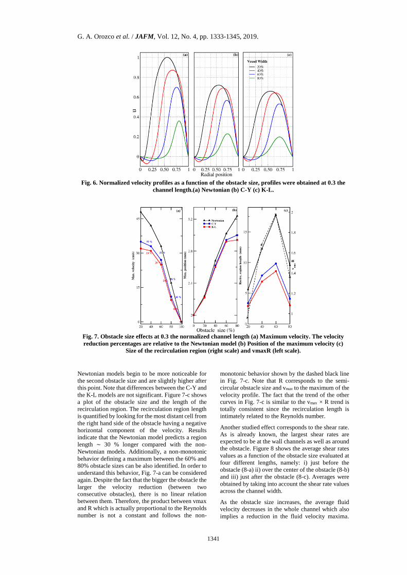
Figure 6 shows the effect of the obstacle size on the

velocity profiles. Four different obstacle sizes were

studied and correspond to radii of 20%, 40%,

60%and 80% the channel width. As previously done,

the velocity values were normalized with respect to

the maximum Newtonian velocity. For this particular

case, simulations were required to satisfy the stricter

condition of 10^{-10} in the equilibrium criterion

given by Eq. (3) . The profiles shown are evaluated

at 0.3 of the channel length. Although numerical

differences were observed evaluating the profile at

different lengths, a similar qualitative trend was

found (not shown).

As the size increases, it is possible to see a reduction

of the velocity that is more pronounced for the

Newtonian model followed by the C-Y and the K-L

models. Also, for all models, maxima are displaced

as a function of the obstacle size, and negative


1340

Fig. 4. Velocity, shear rates and pressure behavior for the Newtonian model in the presence of a semi-

circular obstacle. Plots were coded in the ROOT data analysis framework. All values are shown in

normalized units.

Fig. 5. Velocity profiles for the different rheological models using an obstacle of radius 40% of the

channel width. (a) Newtonian model (b) C-Y model (c) K-L model. The profiles were taken at different

normalized channel lengths before and after the obstacle.

velocities can be observed to be higher in magnitude

for the Newtonian model. The origin of negative

velocities is related to the existence of a recirculation

region, which is produced by the contact between the

fluid and the obstacle surface. This interaction

reduces the fluid kinetic energy and avoids part of it

to overcome the adverse pressure gradient.

Figure 7 quantifies some of the above-mentioned

effects. Figure 7-a shows how the velocity maximum

is reduced as a function of the obstacle size. All

rheological models exhibit a similar trend with

different slopes. All curves are bounded between two

limits, namely, the upper limit for a system without

an obstacle and the lower one for a complete

obstruction. As can be observed, the Newtonian

model has the steepest slopes for nearly all obstacles

sizes. This result can be explained due to the fact that

the highest velocity values are predicted by the

Newtonian model and for a complete constriction all

models should converge to zero. Non-Newtonian

models show a much less pronounced effect for the

first two sizes. However, as the obstacle size

increases, slopes start to be numerically closer.

Differences between Newtonian and C-Y models are

on average ∼ 25% while for K-L and the Newtonian

model difference are on average ∼ 32%.

Figure 7-b, shows the position dependence of the

velocity profiles maxima relative to the obstacle size

at 0.3 of the channel length. The first point refers to

the non-obstacle case where all maxima are located

at the channel center. Contrary to Fig. 7-a,

differences among the Newtonian and non-


1341

Fig. 6. Normalized velocity profiles as a function of the obstacle size, profiles were obtained at 0.3 the

channel length.(a) Newtonian (b) C-Y (c) K-L.

Fig. 7. Obstacle size effects at 0.3 the normalized channel length (a) Maximum velocity. The velocity

reduction percentages are relative to the Newtonian model (b) Position of the maximum velocity (c)

Size of the recirculation region (right scale) and vmaxR (left scale).

Newtonian models begin to be more noticeable for

the second obstacle size and are slightly higher after

this point. Note that differences between the C-Y and

the K-L models are not significant. Figure 7-c shows

a plot of the obstacle size and the length of the

recirculation region. The recirculation region length

is quantified by looking for the most distant cell from

the right hand side of the obstacle having a negative

horizontal component of the velocity. Results

indicate that the Newtonian model predicts a region

length ∼ 30 % longer compared with the non-

Newtonian models. Additionally, a non-monotonic

behavior defining a maximum between the 60% and

80% obstacle sizes can be also identified. In order to

understand this behavior, Fig. 7-a can be considered

again. Despite the fact that the bigger the obstacle the

larger the velocity reduction (between two

consecutive obstacles), there is no linear relation

between them. Therefore, the product between vmax

and R which is actually proportional to the Reynolds

number is not a constant and follows the non-

monotonic behavior shown by the dashed black line

in Fig. 7-c. Note that R corresponds to the semi-

circular obstacle size and vmax to the maximum of the

velocity profile. The fact that the trend of the other

curves in Fig. 7-c is similar to the vmax × R trend is

totally consistent since the recirculation length is

intimately related to the Reynolds number.

Another studied effect corresponds to the shear rate.

As is already known, the largest shear rates are

expected to be at the wall channels as well as around

the obstacle. Figure 8 shows the average shear rates

values as a function of the obstacle size evaluated at

four different lengths, namely: i) just before the

obstacle (8-a) ii) over the center of the obstacle (8-b)

and iii) just after the obstacle (8-c). Averages were

obtained by taking into account the shear rate values

across the channel width.

As the obstacle size increases, the average fluid

velocity decreases in the whole channel which also

implies a reduction in the fluid velocity maxima.


1342

Fig. 8. Average shear rates around the obstacle region. (a) just before the obstacle (b) over the obstacle

(c) just after the obstacle (d) qualitative shear rate profiles across the channel width.

Since the velocity remains zero at the channel walls

and over the obstacle, both velocity changes and

shear rates are lower as well. Fig. 8-a and Fig. 8-c

show how the average shear rates decrease as a

function of the obstacle size for regions away from

the constriction. On the other hand, the largest

velocities are located over the obstacle and define a

velocity profile which drastically changes from the

obstacle wall to the constriction center. As a

consequence, the average shear rate is larger around

the obstacle region and increases as a function of the

obstacle size as shown in Fig. 8-b.

No major differences can be appreciated between the

average shear rate inside and outside the constriction

region for the smallest obstacle. Numerical values

range between 100-180 s−1. However, for the largest

obstacle, at the constriction the average shear rates

increase up to ∼ 400 s−1 while away from it they are

always lower than 80 s−1, depending on the

rheological model. High shear rates, where blood is

supposed to behave as a Newtonian fluid, can be

found at the channel walls and can be even higher in

the constriction region due to the presence of the

obstacle. Figure 8-d qualitatively shows the shear

rates across the channel width for the three regions.

As can be observed, the shear rate is maximum

around the obstacle and significantly reduces after it.

Away from the constriction region, where higher

viscosity values are expected, Newtonian models

will tend to over-predict the results, which is in

agreement with previous computational works

carried out on intracranial aneurysm. (Xiang,

Tremmel, Kolega, Levy, Natarajan, and Meng,

2012) Furthermore, overpredictions of these results

might lead to incorrect estimations when studying

thrombus generation or growth. (Lee, Chiu, and Jen,

1997)

Changes in the position of the maximum velocity

also depends on the shear rate distribution. As

mentioned before, for the non-obstacle case maxima

are expected to be at the channel center, because

shear rates are equal at both channel walls. However,

for the obstacle case, as can be appreciated in Fig. 4-

b and Fig. 8-d (yellow line), shear rates at the

obstacle and on the channel walls are different in

magnitude producing a shift of the maximum

position towards the surface of higher shear rates.

Due to the fact that blood clots, stents or thrombus

might have different shapes. We consequently

wanted to find out about the effect of the obstacle

geometry on the flow. Thus, in addition to the semi-

circular obstacle case, a rectangular shape with a

height side equal to the semi-circle radius and a base

equal to the semi-circle diameter was also

considered. Figure 9 shows a comparison between

the two geometries for the velocity profiles and an

obstacle size of 40% of the channel width. Although

a similar qualitative trend was found between the

geometries, the velocity profiles for the semi-circular

obstacle were ∼ 15% higher.

Higher velocities are expected to be found for the

semi-circular case since over this geometry the flow

has an easier circulation and a lower reduction in the

flow velocity. This behavior is found at all lengths

and it is clearer at the channel outlet profile (blue

line). The obtained differences show that the

geometry has an effect, not only on the velocity

magnitudes, but also on the location of the maximum

velocity. Maximum velocities are closer to the top

wall for the rectangular obstacle.

4. CONCLUSIONS AND PROSPECTS

In this work a quantitative comparison has been

performed of blood flow using several rheological

models in a normal blood channel as well as in the

presence of an obstacle. A new methodology has


1343

Fig. 9. Comparison of the Newtonian velocity profiles using a circular and rectangular geometry.

been proposed in order to simultaneously fit the

parameters belonging to all the studied rheological

models. Following this approach, a new set of

parameters for the C-Y and the K-L models were

determined based on several experimental samples

for a wide range of shear rates. Additionally, it was

found that the Casson model was unable to provide a

good fit when a wide range of shear rates was

included. This indicates that the C-Y and the K-L

models should be considered as better alternatives.

In our opinion any study needs to take into account a

simultaneous fit of the parameters, otherwise, any

comparison will be inconsistent.

Several physical observables have been studied,

namely: velocity profiles, shear rate profiles and the

length of the recirculation region. Among the studied

rheological models, and regardless of the obstacle,

the Newtonian model tends to predict higher

numerical values for all the physical magnitudes.

Although the C-Y and the K-L models show similar

numerical results, the C-Y predictions were always

larger than the K-L ones.

The presence of an obstacle produces for the studied

Reynolds number: a reduction of the fluid velocities

in the whole channel, a loss of symmetry with respect

to the channel center, displacement of the velocity

maxima and the appearance of a re-circulation region

just after the obstacle. The location of the maximum

velocity was found to be different between non-

Newtonian and Newtonian models. The recirculation

region length was found to be non-monotonically

related to the obstacle size and the Newtonian

models predicted the longest lengths. As a

consequence, using Newtonian models might lead to

predictions of higher probabilities of platelet

adhesion to the wall channels and therefore higher

probabilities of a thrombus growth.

The highest shear rate values were found over the

obstacle region and were on average higher for the

Newtonian model. Furthermore, once the obstacle

was placed inside the channel there was a significant

effect on the shear rate distribution. In fact, its

behavior was found to be considerably different

inside and outside the constriction region. For that

reason, a model with a constant viscosity might not

be sufficient to provide a good system description

and hence more detailed models should be used.

Despite the fact that the obstacle effect was included,

it is known that a thrombus implies a complex set of

chemical reactions that account for its formation and

consequent growth. For that reason, a future study

that considers these variables is needed.

Additionally, the variables studied in this work are

not enough to determine the best rheological model

choice. Thus, in order to clarify this issue, more

experimental information such as velocities or shear

rates need to be also included.

5. ACKNOWLEDGMENTS

G. A. Orozco and D. A. Roa Romero, acknowledges

the Universidad Antonio Nari~no for the financial support via the project number 2018-001.

REFERENCES

Anand, M. N., K. Rajagopal and K. R. Rajagopal

(2005). A model for the formation and lysis of

blood clots. Pathophysiology of Haemostasis

and Thrombosis 34(2-3), 109–120.

Ashrafizaadeh, M. and H. Bakhshaei (2009). A

comparison of non-newtonian models for lattice

boltzmann blood flow simulations. Computers

and Mathematics with Applications 58(5),

1045–1054.

Baskurt, O. K. and H. Meisleman (2003). Blood

rheology and hemodynamics. Seminars in

Thrombosis and Hemostasis 29(5), 436–450.

Bate, H. (1977). Blood viscosity at different shear

rates in capillary tubes. Biorheology 14(5-6),

267–275.

Biro, G. P. (1982). Comparison of acute

cardiovascular effects and oxygen-supply

following haemodilution with dextran, stroma-

free haemoglobin solution and fluorocarbon

suspension. Cardiovascular Research 16(4),


1344

194–204.

Bodnár, T., A. Sequeira and M. Prosi (2011). On the

shear-thinning and viscoelastic effects of blood

flow under various flow rates. Applied

Mathematics and Computation 217(11), 5055–

5067.

Box, F. M., R. J. van der Geest, M. C. M. Rutten and

J. H. Reiber (2005). The influence of flow,

vessel diameter, and non-newtonian blood

viscosity on the wall shear stress in a carotid

bifurcation model for unsteady flow.

Investigative Radiology 40(5), 277–294.

Boyd, J., J. M. Buick and S. Green (2007). Analysis

of the casson and carreauyasuda non-newtonian

blood models in steady and oscillatory flows

using the lattice boltzmann method. Physics of

Fluids 19(9), 0931031–09310314.

Brooks, D., J. W. Goodwin and G. V. Seaman

(1970). Interactions among erythrocytes under

shear. Journal of Applied Physiology 28(2),

172–177.

Casson, N. (1959). A flow equation for pigment-oil

suspensions of the printing ink type. In C. Mill

(Ed.), Rheology of Disperse Systems, pp. 84–

104. London, UK: Pergamon Press.

Chien, S. (1970). Shear dependence of effective cell

volume as a determinant of blood viscosity.

Science 168(3934), 977–979.

Chien, S., S. Usami, H. M. Taylor, J. L. Lundberg

and and M. L. Gregersen (1966). Effects of

hematocrit and plasma proteins on human blood

rheology at low shear rates. Journal of Applied

Physiology 21(1), 81–87.

Cho, I. Y. and R. K. Kensey (1991). Effects of the

non-newtonian viscosity of blood on flows in a

diseased arterial vessel. Part i: Steady flows.

Biorheology 28(3-4), 241–262.

Fedosov, D. A., P. Wenxiao, B. Caswell, G.

Gompper and G. E. Karnidiakis (2011).

Predicting human blood viscosity in silico.

Proceedings of the National Academy of

Sciences of the Unites States of America

108(29), 11772–11777.

Fogelson, A. L. and R. D. Guy (2004). Platelet-wall

interactions in continuum models of platelet

thrombosis: formulation and numerical solution.

Mathematical Medicine and Biology 21(4),

293–334.

Gijsen, F. J. H., E. Allanic, F. N. van de Vosse and J.

Jansenn (1999). The influence of the non-

newtonian properties of blood on the flow in

large arteries: unsteady flow in a 90 curved tube.

Journal of Biomechanics 32(7), 705–713.

Gijsen, F. J. H., F. N. van de Vosse and J. Jansenn

(1999). The influence of the non-newtonian

properties of blood on the flow in large arteries:

steady flow in a carotid bifurcation model.

Journal of Biomechanics 32(6), 601–608.

Glaser, R. (2012). Biophysics, An Introduction.

Heidelberg, Germany: Springer.

Ha, H. (2012). Hybrid piv-ptv technique for measuring blood flow in rat mesenteric vessels.

Microvascular Research 84(3), 242–248.

Hathcock, J. (2006). Flow effects on coagulation and

thrombosis. Arteriosclerosis, Thrombosis, and

Vascular Biology 26(8), 1729–1737.

Krüger, T., F. Varnik and D. Raabe (2009). Shear

stress in lattice boltzmann simulations. Physical

Review E 79, 46704–1 – 46704–14.

Lee, D., Y. L. Chiu and C. Jen (1997). Platelet

adhesion onto the wall of a flow chamber with

an obstacle. Biorheology 34(12), 111–126.

Leuprecht, A. and K. Perktold (2001). Computer

simulation of non-newtonian effects on blood

flow in large arteries. Computer Methods in

Biomechanics and Biomedical Engineering

4(2), 149–163.

Liu, Y. and W. K. Liu (2006). Rheology of red blood

cell aggregation by computer simulation.

Journal of Computational Physics 220(1), 139–

154.

Lobanov, A. I. and T. K. Staroszhilova (2005). The

effect of convective flows on blood coagulation

processes. Pathophysiology of Haemostasis and

Thrombosis 34(2-3), 121–134.

Luo, X. Y. and Z. B. Kuang (1992). A study of the

constitutive equation of blood. Journal of

Biomechanics 25(8), 929–934.

Milnor, W. R. (1982). Hemodynamics. Baltimore,

MD: Willians and Wilkins.

Ouared, R. and B. Chopard (2005). Lattice

boltzmann simulations of blood flow: non-

newtonian rheology and clotting processes.

Journal of Statistical Physics 121(1-2), 209–

221.

Perktold, K., R. Peter and M. Resch (1995). Computer-simulation of local blood-flow and

vessel mechanics in a compliant carotidartery

bifurcation model. Journal of Biomechanics

28(7), 845–856.

Pivkin, I. V. and E. G. Karniadakis (2008). Accurate

coarse-grained modeling of red blood cells.

Physicial Review Letters 101(11), 1181051–

1181054.

Robertson, A. M., A. Sequeira and R. G. Owens

(2009). Rheological models for blood. In L.

Formaggia, A. Quarteroni, and A. Veneziani

(Eds.), Cardiovascular Mathematics, Volume 1,

Chapter 6, pp. 211–241. Milan, Italy: Springer-

Verlag.

Skalak, R., S. R. Keller and T. W. Secomb (1981).

Mechanics of blood flow. Journal of

Biomechanical Engineering 103(2), 102–115.

Sorensen, E. N., G. W. Burgreen, W. R. Wagner and

J. F. Antaki (1999a). Computational simulation

of platelet deposition and activation: I. model

development and properties. Annals of


1345

Biomedical Engineering 27(4), 436–448.

Sorensen, E. N., G. W. Burgreen, W. R. Wagner and

J. F. Antaki (1999b). Computational simulation

of platelet deposition and activation: Ii. results

for poiseuille flow over collagen. Annals of

Biomedical Engineering 27(4), 449–458.

Succi, S. (2001). The lattice Boltzmann method for

fluid mechanics and beyond. Oxford, UK:

Clarendon Press.

Tangelder, G. J., D. W. Slaaf, A. M. Muijtjens, E. M.

G. Arts, T., and R. S. Reneman (1986). Velocity

profiles of blood platelets and red blood cells

flowing in arterioles of the rabbit messentery.

Circulation Research 59(5), 505–514.

Wang, C. H. and J. R. Ho (2011). A lattice

Boltzmann approach for the non-newtonian

effect in the blood flow. Computers and

Mathematics with Application 62(1), 75–86.

Weller, F. F. (2008). Platelet deposition in non-

parallel flow. Journal of Mathematical Biology

57(3), 333–359.

Weller, F. F. (2010). A free boundary problem

modeling thrombus growth:modeling

development and numerical simulations using

the level set method. Journal of Mathematical

Biology 61(6), 805–818.

Wootton, D. M., A. S. Popel and B. R. Alevriadou

(2002). An experimental and theoretical study

on the dissolution of mural fibrin clots by tissue-

type plasmonigen activator. Biotechnology and

Bioengineering 77(4), 405–419.

Xiang, J., M. Tremmel, J. Kolega, E. I. Levy, S. K.

Natarajan and H. Meng (2012). Newtonian

viscosity model could overesitmate wall shear

stress in intracanial aneurysm domes and

understimate rupture risk. Hemorrhagic Stroke

4(5), 351–357.

Xu, Z., N. Chen, M. M. Kamocka, E. D. Rosen, and

M. Alber (2008). A multiscale model of

thrombus development. Journal of the Royal

Society Interface 5(24), 705–722.

Zhang, Z. W. and B. Neu (2009). Role of macro-

molecular depletion in red blood cell adhesion.

Biophysics Journal 97(4), 1031–1037.

Zou, Q. and X. He (1997). On pressure and velocity

boundary conditions for the lattice boltzmann

bgk model. Physics of Fluids 9, 1591–1598.

Zydney, A. L., J. D. Oliver III and C. K. Colton

(1991). A constitutive equation for the viscosity

of stored red cell suspensions: Effect of

hematocrit, shear rate, and suspending phase.

Journal of Rheology 35, 1639–1680.

Blood Flow in Channel Constrictions: A Lattice-Boltzmann ...

Documents

Transcript of Blood Flow in Channel Constrictions: A Lattice-Boltzmann ...