arX

iv:c

omp-

gas/

9610

001v

1 2

Oct

199

6

1 Introduction

The Lattice Boltzmann Method (LBM) was introduced in the late 80’s to copewith the two major drawbacks of Lattice Gas Cellular Automata (LGCA), i.e.statistical noise and exponential complexity of the updating rule governing thetime evolution of the cellular automaton (Mc Namara 1988, Higuera & Jimenez1989, Benzi et al. 1992). Ever since, the LBM has undergone progressive re-finements which have brought it to the point where it can compete with mostadvanced computational fluid dynamics (CFD) methods for a wide variety ofproblems, ranging from fully developed, homogeneous incompressible turbu-lence, to low Reynolds number flows in porous media.However, when it comes to complex geometries such as those commonly encoun-tered in many engineering applications, for instance internal flows of automotiveinterest, LBM still lags significantly behind state-of-the art CFD techniques.This is due to the inability of LBM to accommodate any sort of non-uniformityin the spatial distribution of the mesh grid points. This limitation is a directinheritance from LGCA, which are based upon a set of mono-energetic par-ticles (same speed amplitude for the various propagation directions) hoppingsynchronously, in lock-step mode, from site to site according to the direction ofthe discrete speeds. Since the discrete speeds must be the same at any latticesite, a uniform spatial lattice necessarily results.This is in a blatant contrast with the modern CFD methods which are gener-ally capable of accomodating fairly complex meshes. In the attempt to bridgethis gap, a coarse-grained extension of the LBM has been recently introduced(Nannelli 1992).This extension, by borrowing standard ideas from the Finite Volume method,does provide a significant enhancement of the geometrical flexibility of LBM,although, for the sake of simplicity, it was restricted to two dimensional, carte-sian non-uniform grids.In this paper, the two dimensional restriction is lifted and a fully three dimen-sional coarse-grained LBM is developed. Before moving on to the details onhow this is achieved, let us spend some remarks on a further reason why, webelieve, the present study is warranted.It is argued (Boris 1989, Boris et al. 1992) that the increasing availability ofparallel computers is pushing CFD towards a situation of diminishing returnsin terms of trading off computational cost for accuracy. In other words, thequestion is whether it is more effective to increase the grid resolution using alow-order “lean” scheme, rather then striving to save memory using a high-order“heavy” scheme.The LB method is well positioned to attempt a contribution in this direction: itis a low-order explicit scheme (2nd order in space, first in time) which performsextremely well on virtually any parallel architecture. On the other hand, as itstands today, the LB method cannot compete with modern CFD methods insituations where non-uniform stretched mesh are required. In fact, the gap in

1

number of grid points is simply too huge and no argument of better parallelefficiency can really compensate for it. This prompts the need of developingextended LB schemes able to reduce the gap, if not close it altogether.The extension we shall be looking for, should be such as to achieve geometricalflexibility without compromising the outstanding amenability to parallel com-puting to any serious extent. This paper presents the first exploratory effort inthis direction for flows of engineering interest.

2 Short review of Lattice Boltzmann method

The Lattice Boltzmann Equation reads as follows:

fi(~x + ~ci, t + 1) − fi(~x, t) =

b∑

j=1

Ωij(fj − feqj ) (1)

where fi represent the probability of a particle to be moving along direction~ci, Ωij is the scattering matrix between state i and j and feq

j are the localequilibrium populations, expanded to second order in the flow speed ~u to retainconvective effects. Here feq

j is given by (repeated indices are summed upon):

feqi =

ρ

b

(

1 +1

2ci,αuα + 2Qi,αβuαuβ

)

α, β = x, y, z (2)

where Qi,αβ ≡ ci,αci,β− 12δαβ , is the projector upon the i-th speeds, ρ ≡ ∑

i fi isthe flow density, and ~u ≡

∑

i fi~ci/ρ is the hydrodynamic velocity. The discretespeeds ~ci belong to a four-dimensional face centered hypercube (FCHC) definedby |~ci| =

√2, and ci,x + ci,y + ci,z + ci,w = 2 (Frisch et al., 1987).

The equation (1) can be regarded as an explicit finite-difference approximationto a model Boltzmann equation of a BGK type (Qian et al. 1992). Also onecan prove the existence of a H-theorem which guarantees its numerical stabilityin the linear regime (Mach ≪ 1) provided the spectrum of Ωij is confined tothe strip −2 < λ < 0 . As a result, the eigenvalue λ can be tuned to minimizethe viscosity according to the relation

ν = −1

3(1

2+

1

λ)

For further details see the recent review by Qian et al., (1995).The basic merits of LBE are:

• Flexibility in the choice of the collision rules;

• Flexibility in the handling of boundary conditions;

• Ideal amenability to vector/parallel computing;

2

A serious drawback of LBE, as compared to advanced CFD solvers, relatesto the constraint of operating on a uniform, regular mesh. This limitation isparticularly offending for those engineering applications in which a selective dis-tribution of the spatial grid points is required in order to cluster the degrees offreedom there where needed on account of physical and geometrical demands.The main idea proposed in this paper is to overcome the limitation of the uni-form LB scheme based on the two-grid procedure (Nannelli 1992, Succi 1994)described in the next section.

3 LB for a non-uniform grid

Think of two different lattices, Lf and Lc: Lf is a fine-grained uniform latticecorresponding to the usual LB scheme, Lc, instead, is a non-uniform coarserlattice whose cells typically contain several nodes of Lf . The idea is to take thedifferential form of LB Dynamics:

∂tfi + ~ci · ~∇fi =

b∑

j=1

Ωij(fj − feqj ) ≡ ωi (3)

and apply a finite-volume procedure based upon integration of eq. (3) on eachcell of the coarse grid Lc. By straightforward use of Gauss theorem, we obtain

dFi

dt+ Φi = Ωi , i = 1, b (4)

where

Fi =1

Vc

∫

C

fid3x (5)

Φi =1

Vc

∫

∂C

fi(~ci · n)d2x

Ωi =1

Vc

∫

C

ωid3x

Here Fi is the mean population of the macrocell C, Φi the corresponding fluxacross the boundaries of C, and Ωi is the rate of change of Fi due to collisionsoccurring within the cell C.The expression (4) represents a set of Nc ordinary differential equations for theunknowns Fi, Nc being the number of cells of the coarse grid Lc. To closethis system, we need to express the surface fluxes Φi in terms of the cell-valuesFi. This calls for an appropriate interpolation procedure mapping the fine-grain distribution fi onto the coarse-grain distribution Fi. Note that while fi

is defined on the nodes of Lf , Fi is located on the centers of the cells of Lc. Ina formal sense, we can write:

R : Fi → fi (6)

3

where the reconstruction operator R is the (pseudo-)inverse of the averagingoperator A:

A : fi → Fi (7)

operationally defined by eq. (5).Two reconstruction operators have been considered: a piece-wise constant (PWC)and a piece-wise linear (PWL). For the sake of simplicity hereafter we shall re-strict our attention to the case of a cartesian non-uniform grid stretched alongthe z-direction:

∆x = bx · a, ∆y = by · a, ∆z = h(z) · a (8)

where a is the spacing of the uniform fine-grained grid.This extends previous non-uniform LB schemes in three respects: first, thescheme is three dimensional; second, the stretching factors bx, by, h(z) need notbe integers; third, the stretching factor along z need not be a constant.By using piece-wise constant interpolation for the collision operator (local inspace) and piecewise linear for the streaming operator (first-order), we arriveat the following coarse-grained LB equation (Finite Volume LBE, FVLBE forshort):

Fi =

Ni∑

ν=0

Cνi F ν

i +b

∑

j

Ωij(Fj − F eqj ) (9)

where Fi is the mean popolation at time t+∆t, the index ν denotes the macro-cell involved in the piecewice linear interpolation (i.e. F 0

i ≡ Fi), and Cνi are the

coarse-grained streaming coefficents. The scattering matrix Ωij is the same asgiven in eq. 1, and F eq

i is the same as eq. 2. The streaming coefficents Cνi are

given in Appendix for propagation direction ~ci = (0, 0, 1) and ~ci = (1, 0, 1).Consistently with the intents stated in the introduction, the eq.9 achieves geo-metrical flexibility at a minimal price in terms of aptness to parallel computing.Geometrical flexibility is in charge of coarse-grained streaming coefficents Cν

i ,while almost ideal amenability to parallel computing is preserved because withinour piecewise interpolation, the coarse-grained collision is still completely localin space.

4 Turbulent Channel Flow simulations

The FVLBE scheme described in the previous section has been tested for thecase of three dimensional turbulent channel flow. This application is especiallysuited to our purpose, first because it represents the simple instance of a ge-ometry calling for a non-uniform mesh, and second in view of the wide body ofavalaible literature. Two series of simulations have been performed: low resolu-tion (32 × 32 × 100) and moderate resolution (64 × 64 × 128). Let us begin bydescribing the former. Three series of low resolution runs have been performed

4

with varying factors bx, by (see table 1). The mesh-distribution along z is givenby the following 1 − 2 − 1 law,

∆z(k) =

1 for 1 ≤ k ≤ 252 for 26 ≤ k ≤ 751 for 76 ≤ k ≤ 100

corresponding to a channel height H = 150. The initial condition correspondsto a Poiseuille flow along x with average speed U0 = 0.35, perturbed with amultiperiodic divergence free velocity field. The molecular viscosity is ν0 =0.005, corresponding to a nominal Reynolds number Re0 = U0H/2 × ν0 ∼6000. The first outcome of the numerical experiments is that fully developedturbulence is supported only within a restricted time window, lasting up to 5000,15000, 70000 time step for L3, L2, L1 respectively. As a result only L1 lends itselfto a (partial) statistical analysis of the turbulent field. The analysis proceeds asfollows. Based on consolidated wisdom, the velocity field in a turbulent channelflow is expressed as follows:

ux(z) =

zv2

∗

ν, 0 < z < δ

v∗

χlog

(

v∗zν

)

+ v∗d , z > δ(10)

where χ = 0.4 is the Von Karman constant, v∗ a typical turbulent velocity,and d is a calibration constant (d = 5.5 ± 0.5) (Landau). Here δ = ν/v∗ is thewidth of the “viscous sublayer” while for δ ≤ z we have the “inertial sublayer”.The average velocity profiles drawn from the numerical simulation are checkedagainst eq. (10) to produce best fit values of νn, vn

∗, dn where the superscript n

denotes “numerical simulation”. The consistency check consists of comparingνn with the input laminar viscosity ν0, v∗ with the value provided by the wallstress tensor: v2

∗=< ux(0)uz(0) >, and finally dn with the existing literature,

i.e. d = 5.5 ± 0.5. The actual values of νn, vn∗, dn are derived from the slope of

the linear ux versus z plot (v2∗/ν), the slope of the ux versus log(z) plot ( v∗/χ

) and the value of log(ux) at z = 1 (v∗/χ · log(v∗/ν) + dv∗). In order to assessthe grid independence of the numerical results, three mesh-distributions alongz have been examined:Lattice “A”

∆z(k) =

1 for 1 ≤ k ≤ 242 for 25 ≤ k ≤ 751 for 76 ≤ k ≤ 100

Lattice “B”

∆z(k) =

1 for 1 ≤ k ≤ 14from 1.05 to 1.95 for 15 ≤ k ≤ 342 for 35 ≤ k ≤ 65from 1.9 to 1.1 for 66 ≤ k ≤ 851 for 86 ≤ k ≤ 100

5

Lattice “C”

∆z(k) =

1 for 1 ≤ k ≤ 372 for k = 383 for 39 ≤ k ≤ 622 for k = 631 for 64 ≤ k ≤ 100

The time averaged velocity profiles ux(z) are shown in fig.??, fig.??, fig.??,while corresponding best-fit values are reported in table 2. The dashed line infig. ??, corresponds to the analytical profiles, eq. (10), with the min & maxvalues drawn from the numerical experiment. These min & max are obtained byinterpolating the numerical data with a family of straight lines, and then takingthe min & max slopes within this family. The reason for dealing with a familyof straight lines instead of just one, is that there doesn’t appear to be a uniquechoice for the set of numerical data to be included in the best fit procedure.Consequently, by reporting both min and max we intend to provide a measureof the statistical scatter. From these figures we see that the grids “A” and “B”are the best performers, while grid “C” is pretty out of target. No consistencycheck for v∗ is available for these simulations because the turbulence window istoo narrow to allow the collection of a significant statistical sample for the wallstress tensor. In summary, grid A provides similar results as grid B, althoughslightly better in terms of effective viscosity. In either cases, the measuredviscosity is more than twice the laminar one ν0. This is the result of the non-uniform mesh which introduces sharp localized peaks of artificial viscosity in thevicinity of mesh size discontinuities (z= 32 in our case). This effect has beenfound to fade away as the grid resolution is increased (Amati 1994, Succi 1995).In consequence, moderate resolution runs have been performed using grid A.

4.1 Moderate Resolution simulations

These simulations have been performed on a 64 × 64 × 128 grid with scalingfactors bx = 15, by = 8. Mesh points along z have been distributed according tothe following 1 − 2 − 1 law:

∆z(k) =

1 for 1 ≤ k ≤ 322 for 33 ≤ k ≤ 961 for 97 ≤ k ≤ 128

The result is a physical channel of height H = 192, length Lx = 960, and widthLy = 512, i.e. pretty close to the one examined by Moin and coworkers (Moin& Kim 1980, Moin & Kim 1982, Rogers & Moin 1987, Kim et al. 1987, Jimenez& Moin 1991). The main outcome of these simulations is that turbulence issupported for the entire life span of the simulation, that is 2.4× 105 time steps,

6

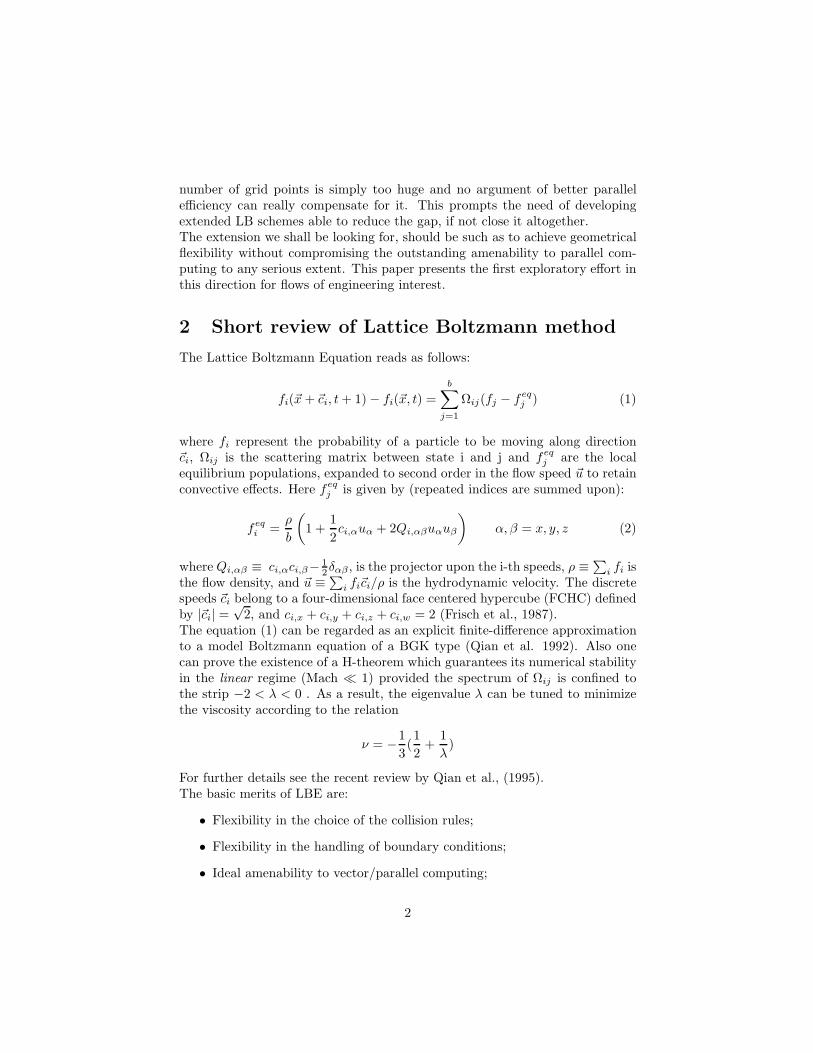
corresponding to about 90 transit time units Lx/U0. This is due to the fact thatthe channel length is now able to support streamwise rolls feeding cross-channelturbulence. These samples have been collected every 53 steps in the interval[105, 2.4 × 105], thus yielding about 2600 profiles for statistical analysis. Theresults are shown in fig. ?? and fig. ??. The numerical best-fit values deducedfrom the analysis are as follows:

νn = 0.013± 0.002, vn∗

= 0.013 ± 0.001, dn = 6.5 ± 0.7 (11)

As a first remark, we see that vn∗

is quite close to the values provided by lowresolution simulations. Also, we note that dn is within the error bars providedby the literature although somewhat (10− 20%) too large. Finally, since turbu-lence is sustained for a significant time-span, wall stress-tensor statistics is alsoavailable. This yields:

v∗ ≡ √< uxuz >|z=0 ∼ 0.012 (12)

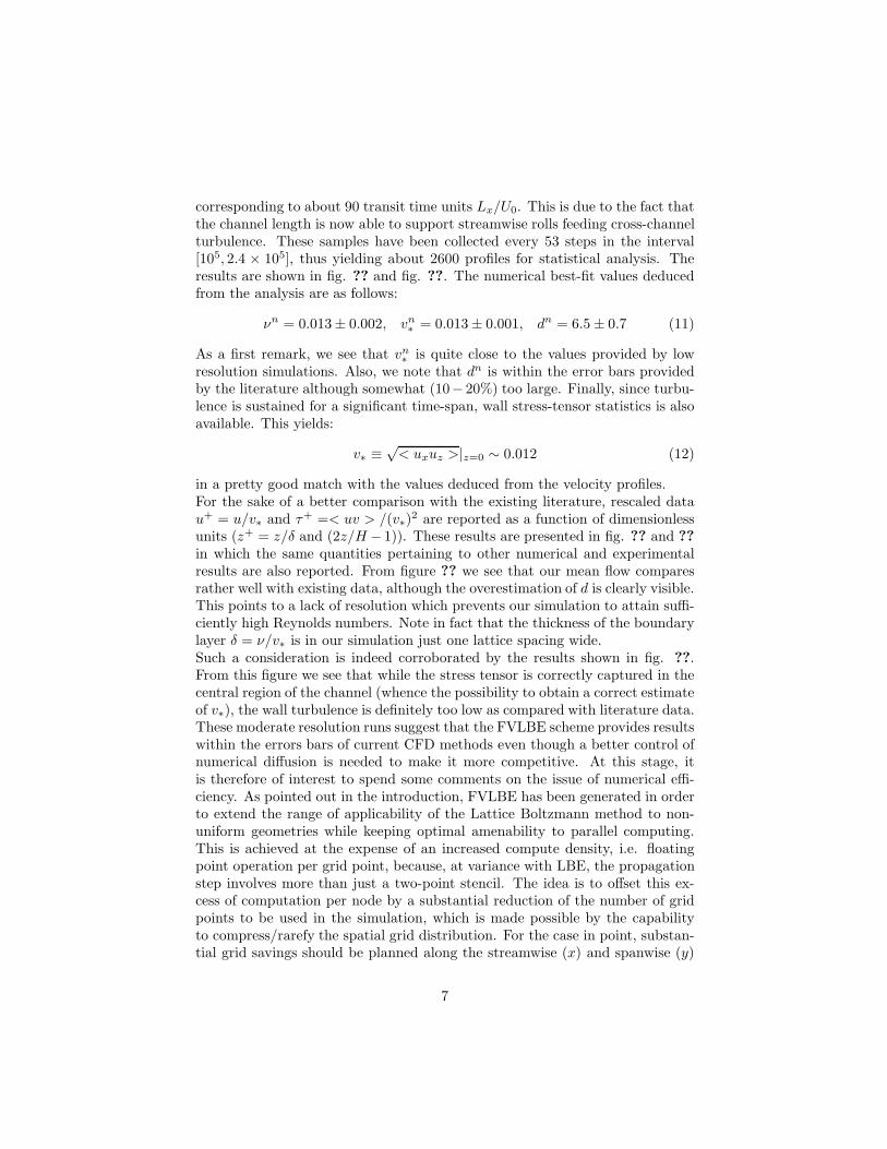
in a pretty good match with the values deduced from the velocity profiles.For the sake of a better comparison with the existing literature, rescaled datau+ = u/v∗ and τ+ =< uv > /(v∗)

2 are reported as a function of dimensionlessunits (z+ = z/δ and (2z/H − 1)). These results are presented in fig. ?? and ??

in which the same quantities pertaining to other numerical and experimentalresults are also reported. From figure ?? we see that our mean flow comparesrather well with existing data, although the overestimation of d is clearly visible.This points to a lack of resolution which prevents our simulation to attain suffi-ciently high Reynolds numbers. Note in fact that the thickness of the boundarylayer δ = ν/v∗ is in our simulation just one lattice spacing wide.Such a consideration is indeed corroborated by the results shown in fig. ??.From this figure we see that while the stress tensor is correctly captured in thecentral region of the channel (whence the possibility to obtain a correct estimateof v∗), the wall turbulence is definitely too low as compared with literature data.These moderate resolution runs suggest that the FVLBE scheme provides resultswithin the errors bars of current CFD methods even though a better control ofnumerical diffusion is needed to make it more competitive. At this stage, itis therefore of interest to spend some comments on the issue of numerical effi-ciency. As pointed out in the introduction, FVLBE has been generated in orderto extend the range of applicability of the Lattice Boltzmann method to non-uniform geometries while keeping optimal amenability to parallel computing.This is achieved at the expense of an increased compute density, i.e. floatingpoint operation per grid point, because, at variance with LBE, the propagationstep involves more than just a two-point stencil. The idea is to offset this ex-cess of computation per node by a substantial reduction of the number of gridpoints to be used in the simulation, which is made possible by the capabilityto compress/rarefy the spatial grid distribution. For the case in point, substan-tial grid savings should be planned along the streamwise (x) and spanwise (y)

7

direction where relatively long-wavelength structures are expected to arise ascompared to cross-flow (z) eddies. For the present 64 × 64 × 128 simulation,each time step takes about 5 second CPU time on a IBM RISC/6000 mod.580.This corresponds to about 10µs per grid point per step, to be compared withroughly 3µs taken by a uniform LBE. These figures reflect approximately theincrease in the number of floating point operation per grid point: about 1000for FVLBE and 500 for LBE. This factor two is largely overcompensated bythe much larger size accessible to FVLBE, i.e. Lx = 960, Ly = 512, H = 192,corresponding to a gain factor of

512

64· 960

64· 192

128= 180 (13)

i.e. about two orders of magnitude. Indeed the channel flow simulation pre-sented in this paper would be simply unfeasible with a plain LBE scheme, forthe latter would take about 30000 CPU seconds per time step, and about 150Gbyte of storage!To date, the largest channel flow simulation we have been also able to per-form with a uniform LB scheme is a 432 × 144 × 288 (1.7 GB) correspondingto Re ≃ 3000, using the 512 processor Quadrics Machine (Bartoloni et al.,1993) Although the parallel performance is exceedingly encouraging (parallelefficiency 54 vs. 64, as can be seen in fig.??, Amati et al., 1996). It is clear thatparallel computing alone cannot make up for the overdemand of computationalresources raised by uniform LB scheme.Our code is almost a factor ten faster than modern semi-implicit CFD methods(compare our 5 s/step on a 64× 64× 128 with a 25 s/step on a 32× 64× 97, seeOrlandi, 1995) but the quality of the results is correspondingly less satisfatory.Both gaps are likely to close up once better interpolators are in place. At thisstage, only aptness to parallel computing will make the difference.

5 Conclusions

By borrowing standard techniques from the finite volume method, a low ordercoarse-grain three dimensional LB scheme has been developed.This scheme basically preserves the outstanding amenability to parallel comput-ing of the uniform LB scheme, while giving access to a much larger Reynoldsnumber class of flows. Actual numerical simulation do, however, reveal thatthe large-scales (the resolved ones) display less turbulent activity than expectedon the basis of the nominal Reynolds number. This means that, while mark-ing a singificant stride forward with respect to the uniform scheme, the presentcoarse-grained LB still lags behind state-of-art CFD methods.A plausible explanation is that our low order interpolator (piecewise constantfor collision operator, and piecewise linear for the streaming operator) doesachieve locality (hence aptness to parallel computing) much at the expense of

8

accuracy. Future work shall then focus on the development of better interpo-lation schemes, possibly in the spirit of Monotone Interpolated Large EddiesSimulation (MILES).In principle there is no reason why the basic advantages of LBM, i.e. handytreatment of complex boundary conditions and outstanding amenability to par-allel computing, should not carry over into FVLBE. Should this be the case,FVLBE may represent a fairly competitive tool for the numerical investigationof inhomogenous turbulent flows on highly parallel machines.

6 Acknowledgements

The authors are indebted to Prof. V. Yakhot, Y. H. Qian and S. Orszag forilluminating discussions.Prof. P. Orlandi is kindly acknowledged for providing literature data reportedin Figs. ??, ??. G.A. would to acknowledge the hospitality of IBM ECSECwhere numerical work has been performed.Parallel simulations were performed on the ENEA Quadrics machine.

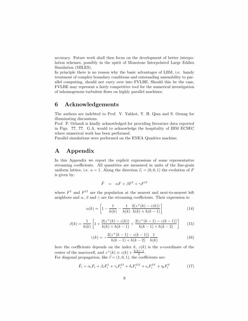
A Appendix

In this Appendix we report the explicit expressions of some representativestreaming coefficients. All quantities are measured in units of the fine-grainuniform lattice, i.e. a = 1. Along the direction ~ci = (0, 0, 1) the evolution of Fis given by:

F = αF + βF I + γF II

where F I and F II are the population at the nearest and next-to-nearest leftneighbors and α, β and γ are the streaming coefficients. Their expression is:

α(k) =

[

1 − 1

h(k)− 1

h(k)

2(z+(k) − z(k))

h(k) + h(k − 1)

]

(14)

β(k) =1

h(k)

[

1 +2(z+(k) − z(k))

h(k) + h(k − 1)+

2(z+(k − 1) − z(k − 1))

h(k − 1) + h(k − 2)

]

(15)

γ(k) = −2(z+(k − 1) − z(k − 1))

h(k − 1) + h(k − 2)

1

h(k)(16)

here the coefficients depends on the index k, z(k) is the z-coordinate of the

center of the macrocell, and z+(k) ≡ z(k) + h(k)−12 .

For diagonal propagation, like ~c = (1, 0, 1), the coefficients are:

Fi = αiFi + βiFIi + γiF

IIi + δiF

IIIi + ǫiF

IVi + ηiF

Vi (17)

9

αi =

[

1 − (bx + h(k) − 1)

bxh(k)

]

+bx − 1

2

bxh(k)

[

2(z−(k) − z(k))

h(k) + h(k − 1)

]

(18)

− h(k) − 12

bxh(k)

[

(x+(k) − x(k))

bx

]

βi =bx − 1

2

bxh(k)+

bx − 12

bxh(k)

[

2(z−(k) − z(k))

h(k) + h(k − 1)

]

+ (19)

+bx − 1

2

bxh(k)

[

2(z−(k + 1) − z(k + 1))

h(k + 1) + h(k)

]

γi = − bx − 12

bxh(k)

[

2(z−(k + 1) − z(k + 1))

h(k + 1) + h(k)

]

(20)

δi =h(k) − 1

2

bxh(k)+

h(k) − 12

bxh(k)

[

(x+(i) − x(i))

bx

]

+ (21)

+h(k) − 1

2

bxh(k)

[

(x+(i + 1) − x(i + 1))

bx

]

ǫi = −h(k) − 12

bxh(k)

[

(x+(i + 1) − x(i + 1))

bx

]

(22)

ηi =1

bxh(k)(23)

10

References

[1] G. Amati; Tesi di Laurea, Physics Dept.,Univ. “La Sapienza” Rome ,(1994)

[2] G. Amati, S. Succi, R. Benzi, R. Piva; Proceedings of Parallel CFD 1996,

Capri, to appear , (1996)

[3] R. Benzi, S. Succi, M. Vergassola; Physics Reports 222 , 3, 147-196 (1992)

[4] J.P. Boris; Annual Review Fluids Mechanics 21 345-385 (1989)

[5] J.P. Boris, F.F. Grinstein, E.S. Oran, R.L. Kolbe; Fluid Dynamic Research

10 199-228 (1992)

[6] A. Bartoloni et al.; Int. J. Mod. Phys. C4 969 (1993)

[7] U. Frisch, D. d’Humieres, B. Hasslacher, P. Lallemand, Y. Pomeau,J. P. Rivet; Complex Systems 1, 649-707 (1987)

[8] F. Higuera, J. Jimenez; Europhysics Letters 9, 663 (1989)

[9] J. Jimenez, P. Moin; Journal of Fluid Mechanics 225, 213-240 (1991)

[10] J. Kim, P. Moin, R. Moser; Journal of Fluid Mechanics 177, 133-166(1987)

[11] G. Mc Namara, G. Zanetti; Physics Rev. Letters 61 , 2332 (1988)

[12] P. Moin, J. Kim; Journal of Computational Physics 35, 381-392 (1980)

[13] P. Moin, J. Kim; Journal of Fluid Mechanics 117, 341-377 (1982)

[14] F. Nannelli, S. Succi; Journal Statistical Physics 68 , 3 (1992)

[15] P. Orlandi; Journal of Non-Newtonian Fluid Mechanics 60 , 277-301 (1995)

[16] Y.H. Qian, D. d’Humieres, P. Lallemand; Europhysics Letters 17 , 479-484(1992)

[17] Y.H. Qian, S. Succi, S. Orszag; Annual Review of Computational Physics

III , 195 (1995)

[18] M.M. Rogers, P. Moin,; Journal of Fluid Mechanics 176, 33-66 (1987)

[19] S. Succi, F. Nannelli; Transport Theory and Statistical Physics 23 , 163-171(1994)

[20] S. Succi, G. Amati, R. Benzi; Journal of Statistical Physics 81, 1/2, 5(1995)

[21] T. Wei, W.W. Willmarth; Journal of Fluid Mechanics 204 , 57-95 (1989)

11