Journal of Computational Physics 228 (2009) 983–999

Contents lists available at ScienceDirect

Journal of Computational Physics

journal homepage: www.elsevier .com/locate / jcp

Lattice Boltzmann simulations of 2D laminar flows past twotandem cylinders

Alberto Mussa a, Pietro Asinari a,*, Li-Shi Luo b

a Department of Energetics, Politecnico di Torino, Torino 10129, Italyb Department of Mathematics and Statistics and Center for Computational Sciences, Old Dominion University, Norfolk, VA 23529, USA

a r t i c l e i n f o

Article history:Received 27 February 2008Received in revised form 2 October 2008Accepted 6 October 2008Available online 17 October 2008

Keywords:Lattice Boltzmann equationBoundary conditionsGrid stretchingFlow past tandem cylinders

0021-9991/$ - see front matter � 2008 Elsevier Incdoi:10.1016/j.jcp.2008.10.010

* Corresponding author. Tel.: +39 011 090 4520;E-mail addresses: pietro.asinari@polito.it (P. AsinURLs: http://staff.polito.it/pietro.asinari (P. Asina

a b s t r a c t

We apply the lattice Boltzmann equation (LBE) with multiple-relaxation-time (MRT) colli-sion model to simulate laminar flows in two-dimensions (2D). In order to simulate flows inan unbounded domain with the LBE method, we need to address two issues: stretched non-uniform mesh and inflow and outflow boundary conditions. We use the interpolated gridstretching method to address the need of non-uniform mesh. We demonstrate that variousinflow and outflow boundary conditions can be easily and consistently realized with theMRT-LBE. The MRT-LBE with non-uniform stretched grids is first validated with a numberof test cases: the Poiseuille flow, the flow past a cylinder asymmetrically placed in a chan-nel, and the flow past a cylinder in an unbounded domain. We use the LBE method to sim-ulate the flow past two tandem cylinders in an unbounded domain with Re = 100. Ourresults agree well with existing ones. Through this work we demonstrate the effectivenessof the MRT-LBE method with grid stretching.

� 2008 Elsevier Inc. All rights reserved.

1. Introduction

In recent years the lattice Boltzmann equation (LBE) has become a viable means for computational fluid dynamics (CFD)(cf. [1] and references therein). As opposed to conventional CFD methods based on direct discretizations of the Navier–Stokesequations, the LBE method is derived from the Boltzmann equation and kinetic theory [2,3]. The kinetic origin of the LBEmethod differentiates it from conventional CFD methods in several ways. In the LBE method, one deals with the discretizedparticle velocity distribution functions ffig instead of the hydrodynamic variables. Therefore, one must also deal with theboundary conditions for the distribution functions ffig instead of that for the hydrodynamic variables. This kinetic natureof boundary conditions in the LBE method has some times caused confusions and the boundary conditions in the LBE arestill a topic of active research.

The most popular LBE implementation of the Dirichlet boundary conditions on the flow velocity u or pressure p is thebounce-back (BB) boundary conditions (BC). When the bounce-back boundary conditions are coupled with the simple latticeBhatnagar–Gross–Krook (BGK) collision model with one single relaxation parameter s, the exact location where the Dirichletboundary conditions for u or p are satisfied depends on the viscosity m (or the relaxation parameter s) [4–8]. This problem inthe lattice BGK (LBGK) equation with the bounce-back BCs has generate numerous papers (e.g. [9–15]). Unfortunately, noneof these works provides a rigorous analysis of or a systematic remedy to the problem due to inaccurate BB-BCs with the LBGK

. All rights reserved.

fax: +39 011 090 4499.ari), lluo@odu.edu (L.-S. Luo).ri), http://www.lions.odu.edu/~lluo (L.-S. Luo).

984 A. Mussa et al. / Journal of Computational Physics 228 (2009) 983–999

model, in spite of the fact that this problem can be analyzed [4–7] and removed [16,7,8] by using the lattice Boltzmannequation with the multiple-relaxation-time (MRT) models [17–20] and improved boundary conditions [16,7,8]. It shouldalso be noted that asymptotic analysis [21,22] has been used to address this problem in LBE [23].

In addition to flow-solid boundary conditions, LBE implementations of various inflow and outflow boundary conditionshave been considered. Various approaches have been proposed previously in the context of the LBGK equation [9,10,13,14].In flow simulations, boundary conditions only specify the values of hydrodynamic variables at boundaries. However, hydro-dynamic boundary conditions are insufficient for the lattice Boltzmann equation, because the distribution functions ffig havenon-equilibrium moments which are not specified by the values of hydrodynamic variables. Similarly, hydrodynamic initialconditions are insufficient to completely specify the LBE initial conditions but can be solved by an iterative procedure [24]. Inthis work we will demonstrate the inflow and outflow boundary conditions of either Dirichlet or Neumann type can be easilyand consistently realized with the MRT-LBE method.

The LBE method usually employs uniform Cartesian meshes in both two and three dimensions. To be computationally effi-cient, non-uniform and adaptive meshes must be used. To this end, two approaches have been used in the LBE: the gridrefinement [15,25,26] and the interpolated grid stretching [27,2,28]. In grid refinement, Cartesian meshes are used, and gridspacing is divided by an integer, which is usually a power of 2, to the next refined grid level. Interpolations are used at theinterface between two connected meshes of different grid spacings, and at solid boundaries [29,8]. With the interpolated gridstretching method, one can use body-fitted meshes [30,31]. Except at flow-solid boundaries, interpolations have to be usedthroughout the entire mesh where the discretized distribution functions ffig cannot be propagated exactly from one grid toanother in the advection process. The simple bounce-back boundary conditions can be used with body-fitted meshes. Wewill use the latter approach, i.e., the interpolated grid stretching, in the present work.

In this paper we intend to use the LBE method to simulate laminar flows past two tandem cylinders in an unboundeddomain in two-dimensions (2D). We shall restrict ourselves to the athermal (or isothermal) LBE models, in which the inter-nal energy is not a conserved quantity. The main objective of this work is to investigate the effectiveness of the MRT-LBEwith non-uniformly stretched grids for flow simulations. Implementations of inflow and outflow boundary conditions withthe MRT-LBE method will also be validated through a number of test cases.

The remainder of this paper is organized as follows. We discuss the LBE method in Section 2, including descriptions ofthe MRT-LBE method, the interpolated bounce-back boundary conditions for arbitrary curved boundaries, inflow and out-flow boundary conditions, force evaluation at flow-solid boundaries, and non-uniform grid stretching method. To validatethe grid stretching method and inflow and outflow boundary conditions, we provide a number of test cases in Section 3.These test cases include: the Poiseuille flow, the flow past a cylinder asymmetrically placed in a channel at the Reynoldsnumber Re = 20 and 100 [32], and the flow past a cylinder in an unbounded domain. In Section 4 we present the LBE re-sults for the flow past two tandem cylinders in an unbounded domain with Re = 100 [33–40]. We will compare our resultswith existing ones obtained with conventional Navier–Stokes solvers [33,37,38]. Finally we conclude the paper with Sec-tion 5.

2. Numerical method

2.1. Multiple-relaxation-time lattice Boltzmann method

We will use the lattice Boltzmann equation with the multiple-relaxation-time (MRT) collision model [17,18,20],

fðxj þ cdt; tn þ dtÞ ¼ fðxj; tnÞ �M�1 � S � ½m�mðeqÞðq;uÞ�ðxj; tnÞ; ð1Þ

where q and u are the macroscopic density and velocity, respectively, the boldface symbols such as f denote Q-tuple vectors,and Q is the number of discrete velocities:

f :¼ ðf0; f1; . . . ; fQ�1ÞT;

fðxj þ cdtÞ :¼ ðf0ðxjÞ; f1ðxj þ c1dtÞ; . . . ; fQ�1ðxj þ cQ�1dtÞÞT;

m :¼ ðm0;m1; . . . ;mQ�1ÞT;

mðeqÞ :¼ ðmðeqÞ0 ;mðeqÞ

1 ; . . . ;mðeqÞQ�1Þ

T;

where T denotes the transpose operator.We will use the nine velocity model (D2Q9 model), of which the discrete velocities are: c0 ¼ ð0;0Þ, ci ¼ ð�1; 0Þc and

ð0;�1Þc, for i = 1–4, and ci ¼ ð�1;�1Þc, for i = 5–8, where c :¼ dx=dt , and dx and dt are the lattice constant (or grid spacing)and time step size, respectively [2,3,18].

With the following specific order of the moments [18]:

m :¼ ðq; e; �;ux; qx;uy; qy;pxx;pxyÞT;

where q is the fluid density (zeroth-order velocity moment), u the velocity (first-order moments), pxx and pxy are the stresses(second-order moment) and q is related to the heat flux (third-order moments), the transform matrix M is given by [18]

A. Mussa et al. / Journal of Computational Physics 228 (2009) 983–999 985

M ¼

1 1 1 1 1 1 1 1 1

�4 �1 �1 �1 �1 2 2 2 2

4 �2 �2 �2 �2 1 1 1 1

0 1 0 �1 0 1 �1 �1 1

0 �2 0 2 0 1 �1 �1 1

0 0 1 0 �1 1 1 �1 �1

0 0 �2 0 2 1 1 �1 �1

0 1 �1 1 �1 0 0 0 0

0 0 0 0 0 1 �1 1 �1

0BBBBBBBBBBBBBBBBBBBBB@

1CCCCCCCCCCCCCCCCCCCCCA

: ð2Þ

The matrix M maps the distribution functions to its moments:

m ¼ M � f; f ¼ M�1 �m: ð3Þ

The labeling of the discrete velocity set fcig is uniquely defined by the rows 4 and 6 in M corresponding to cix and ciy, respec-tively. For the construction of M and detailed description of the moments, we refer readers to the work by d’Humières et al.[18,20].

The diagonal matrix S of relaxation rates fsig is given by

S ¼ diagð0; s2; s3;0; s5;0; s7; s8; s9Þ; ð4Þ

where the relaxation rates s8 ¼ s9 ¼ sm ¼ 1=s determines the dimensionless viscosity of the model:

m ¼ 13

s� 12

� �cdx; ð5Þ

where c :¼ dx=dt . Since the parameter s is dimensionless, then the physical viscosity is proportional to a scaling factor,depending on the adopted grid size and time step (diffusion scaling is assumed). Other relaxation rates s2, s3 ands5 ¼ s7 ¼ sq are usually determined by linear stability of the model [18]. In addition, the no-slip boundary conditions will alsodetermine the choice of s5 ¼ s7 [7,8].

In Eq. (1), the equilibria for the non-conserved moments for the D2Q9 model are

eðeqÞ ¼ �2dqþ 3j � j; eðeqÞ ¼ dq� 3j � j; ð6aÞqðeqÞ

x ¼ �jx; qðeqÞy ¼ �jy; ð6bÞ

pðeqÞxx ¼ j2

x � j2y ; pðeqÞ

xy ¼ jxjy; ð6cÞ

where dq is the density fluctuation, q ¼ �qþ dq and �q ¼ 1, j :¼ ðjx; jyÞ ¼ ð�qux; �quyÞ ¼ ðux;uyÞ is the flow momentum. Here theapproximation for incompressible flows has been used [41], i.e., the coupling between the density fluctuation dq and the flowvelocity u is neglected in m(eq). Note that the equilibria of the conserved moments (q and j :¼ qu) are equal to the conservedmoments themselves. The above equilibria m(eq) are equivalent to the following equilibrium distribution functions:

f ðeqÞi ¼ wi dqþ ðci � uÞ

RTþ 1

2ðci � uÞ2

ðRTÞ2� u � u

RT

" #( ); ð7Þ

where T is the temperature of the flow (assumed constant), R is the specific gas constant and RT represents the internal en-ergy of the fluid, which is a constant for isothermal flows considered here. In the LBE model we use here, RT ¼ c2=3 [2,3,18].For the D2Q9 model, the coefficients w0 ¼ 4=9, wi ¼ 1=9 for kcik ¼ 1, i = 1–4, and wi ¼ 1=36 for kcik ¼

ffiffiffi2p

, i = 5–8.

2.2. No-slip boundary conditions for curved boundaries

We will use the interpolated bounce-back (IBB) boundary conditions (BCs) to model the no-slip fluid–solid boundary con-ditions with curved boundaries [29]. The bounce-back boundary conditions are based on the intuitive picture that a particlereverses its momentum when colliding with a solid wall at the rest. If the wall is moving with a certain velocity uw, a particlecolliding with the wall should also gain additional momentum from the wall. Based on this intuitive picture, as illustrated inFig. 1, if the wall is located one-half grid spacing beyond the last node rA in flow domain, then a particle with velocity c1 atnode rA and time tn collides with the wall at rw, reverses its momentum, and returns to rA. Therefore, when the boundarylocation is not precisely located at dx=2 beyond the last flow node, interpolations or other means must be used to reconstructthe distribution functions at the desirable nodes in flow domain.

The flow nodes adjacent to a solid boundary have links connecting these nodes to their neighboring solid or boundarynodes beyond the flow domain. These links intersect with the boundary so that part of them lie inside the flow domain

Fig. 1. Illustration of the bounce-back (BB) boundary conditions (BCs). (a) q = 1/2, the ‘‘perfect” BB-BCs without interpolation. (b) q < 1/2, the BB-BCs withinterpolations before the collision with the wall located at rw. (c) q P 1=2, the BB-BCs with interpolations after the collision with the wall.

986 A. Mussa et al. / Journal of Computational Physics 228 (2009) 983–999

and part of them are outside, as illustrated by the link between rA and rs in Fig. 1. Define the parameter q as the fraction of alink between a flow node and a boundary node which lies in flow domain as

q :¼ krA � rwkkrA � rsk

; ð8Þ

as depicted in Fig. 1, then one has to treat the following two scenarios separately:

� when q < 12, fiðrDÞ can be constructed from the fi’s in the nearby nodes before the bounce-back collision, so that f�ıðrAÞ is

obtained after the bounce-back collision with the wall located at rw;� when q P 1

2, f�ıðr AÞ is obtained with f�ıðrDÞ after the bounce-back collision and f�ı at other nearby nodes;

where c�ı :¼ �ci is assumed to be the bounced back particle velocity.To reconstruct the distribution functions f�ıðrAÞ entering the flow domain from boundary nodes, we can use either the lin-

ear interpolations:

f�ıðrA; tnþ1Þ ¼ ð1� 2qÞfiðrA; tnþ1Þ þ 2qf �i ðrA; tnÞ; q < 1=2; ð9aÞ

f�ıðrA; tnþ1Þ ¼ð2q� 1Þ

2qf ��ı ðrA; tnÞ þ

12q

f �i ðrA; tnÞ; q P 1=2; ð9bÞ

or the quadratic interpolations:

f�ıðrA; tn þ dtÞ ¼ qð1þ 2qÞf �i ðrA; tnÞ þ ð1� 4q2Þf �i ðrA � cidt; tnÞ þ qð2q� 1Þf �i ðrA � 2cidt ; tnÞ; 0 < q < 1=2; ð10aÞ

f�ıðrA; tn þ dtÞ ¼1

qð1þ 2qÞ f�i ðrA; tnÞ þ

ð2q� 1Þq

f ��ı ðrA; tnÞ þð1� 2qÞð1þ 2qÞ f

��ı ðrA � cidt; tnÞ; 1=2 6 q < 1; ð10bÞ

where f �i denotes the post-collision distribution function. It must be stressed that q = 0 and q = 1 are singular cases. Whenq = 1/2, both the linear and quadratic interpolated bounce-back boundary conditions reduce to the original bounce-backboundary conditions:

f�ıðrA; tnþ1Þ ¼ f �i ðrA; tnÞ:

While the bounce-back boundary conditions are the most often used, they are also misunderstood or misinterpreted veryoften. By no means the intuitive picture illustrated in Fig. 1 should be taken literally. The precise location where the no-slipboundary conditions are satisfied is model dependent. For the incompressible Poiseuille flow with its boundaries parallel to alattice axis, it can be shown analytically that the no-slip boundary location is precisely one-half lattice spacing beyond thelast flow node if and only if the following relation is satisfied [5,7]:

A. Mussa et al. / Journal of Computational Physics 228 (2009) 983–999 987

sq ¼ 8ð2� smÞð8� smÞ

; ð11Þ

where sm ¼ s8 ¼ s9 ¼ 1=s is the relaxation rate for pxx and pxy which also determines the shear viscosity m given by Eq. (5) andsq ¼ s5 ¼ s7 is the relaxation rate for q ¼ ðqx; qyÞ. Obviously, such a relationship cannot be satisfied by the lattice BGK equa-tion with the single-relaxation-time collision model, therefore the no-slip boundary location depends on the relaxationparameter s in lattice BGK models [7,42,8].

2.3. Inflow and outflow boundary conditions

The inflow and outflow boundary conditions used in the LBE simulations are either the Dirichlet or Neumann types for thehydrodynamic variables p (or q) and u. In an athermal LBE model of Q velocities in d dimensions, we have (d + 1) conservedvariables, i.e., q and qu, among all Q moments. The hydrodynamic boundary conditions for q and qu do not specify theboundary conditions for the remaining ðQ � d� 1Þ non-conserved or kinetic moments, which are important in the LBE.We will discuss how to consistently treat these kinetic moments in the boundary conditions.

The Dirichlet boundary conditions for either velocity u or pressure p can be realized by the procedures described bellow.Assume a 2D computational domain is covered by a rectangular uniform mesh without stretching, with nodes labeled byindex (i, j), i 2 f1;2; . . . ;Nxg and j 2 f1;2; . . . ;Nyg, and the streamwise direction is along the x-axis. As an example, we willuse the inlet velocity boundary conditions at the left of the mesh to illustrate the proposed boundary conditions. The velocityuði ¼ 1; jÞ ¼ uinðjÞ is imposed at the inlet i ¼ 1. While the velocity uði ¼ 1; jÞ ¼ uinðjÞ at i = 1 remained intact, all other mo-ments are copied from the line i = 2 adjacent to the inlet. These moments are then transformed to the distribution functionsfði ¼ 1; jÞ, which are used as the boundary conditions at the inlet. Thus the velocity boundary condition at the inlet i = 1 canbe written as

fði ¼ 1; jÞ ¼ M�1 �m�ði ¼ 2; jÞju¼uin; ð12Þ

where m* denotes the post-collision moments. Similarly, the pressure boundary condition pði ¼ 1; jÞ ¼ pinðjÞ can be realizedas

fði ¼ 1; jÞ ¼ M�1 �m�ði ¼ 2; jÞjq¼qin; ð13Þ

where qin ¼ pin=c2s . In the proposed boundary conditions described above, all the non-equilibrium moments are generated in

the flow domain through the evolution process consistent with the flow, only the hydrodynamic variables, either u orq, relevantto specific boundary conditions are imposed at the boundary. Therefore, as the flow develops, non-equilibrium (non-conserved)moments and the equilibrium moments which are not imposed by the given boundary conditions at the boundary are expectedto consistently evolve according to flow dynamics. In the proposed boundary conditions, no complicated interpolations orextrapolations are needed. For simulations in this work, we usually use the velocity boundary conditions at the inlet, and theconstant pressure boundary condition at the outlet:

qout ¼ constant:

We will compare the proposed boundary conditions described above with the non-equilibrium bounce-back boundary con-ditions [14], in which the velocity boundary conditions uði ¼ 1; jÞ ¼ u inðjÞ at the inlet are realized as

f�kði ¼ 1; jÞ ¼ fkði ¼ 2; jÞ � f ðeqÞk ði ¼ 2; jÞ þ f ðeqÞ

�kði ¼ 2; jÞju¼uinðjÞ ¼ fkði ¼ 2; jÞ � 3wkck � ½uði ¼ 2; jÞ þ uinðjÞ�; ð14Þ

where f�k is the distribution function corresponding to the discrete velocity c�k, and c�k :¼ �ck is an incoming discrete particlevelocity with respect to the boundary at i = 1, i.e., those velocities with positive x component ðc�kx > 0Þ hence ff�kði ¼ 1; jÞg arethe incoming distribution functions. In the above derivation, we have assumed the incompressible LBE model [41] with theequilibria of Eq. (7). Similarly, when the pressure boundary condition pði ¼ 1; jÞ ¼ pinðjÞ is imposed at the entrance, or equiv-alently qði ¼ 1; jÞ ¼ qinðjÞ through q ¼ p=c2

s , the non-equilibrium bounce-back boundary conditions are

f�kði ¼ 1; jÞ ¼ fkði ¼ 2; jÞ �wk½qði ¼ 2; jÞ � qinðjÞ� � 6wkck � uði ¼ 2; jÞ: ð15Þ

Another way of implementing a constant pressure p ¼ pout ðq ¼ qout ¼ pout=c2s Þ at the outlet i ¼ Nx is to impose equilibrium

distributions:

fkði ¼ Nx; jÞ ¼ f ðeqÞk ðq ¼ qout;u ¼ uði ¼ Nx � 1; jÞÞ: ð16Þ

With the MRT-LBE, the inflow and outflow boundary conditions discussed above are particularly easy to implement. Afteradvection and collision, the moments at i = 2 are copy to i = 1, then either the velocity u or the density q are reset accordingto given boundary conditions, while the rest of the moments are remained intact. The moments fmig are transformed back tothe distribution functions ffig, which carry the information imposed by the boundary conditions to flow domain. This differsfrom the approach that sets the distribution functions ffig to their equilibria ff ðeqÞ

i g with the specified values of hydrody-namic variables at the boundaries [9] or that uses extrapolations to obtain non-equilibrium distribution functions [10,13].The proposed approach will be tested numerically in Section 3.1.

988 A. Mussa et al. / Journal of Computational Physics 228 (2009) 983–999

2.4. Force evaluation at flow-solid boundaries

Two methods to compute hydrodynamic forces on a flow-solid boundary in the lattice Boltzmann simulations are used.The first method is to compute the pressure and stresses at the flow-solid boundary and then to integrate the forces over theentire boundary. For arbitrary curved boundaries, the hydrodynamic forces at boundary can be obtained by interpolatingeither the pressure and velocity fields from flow nodes to boundary locations [30,31,43–45], or the distribution functionsto compute the local stresses.

The second method is the momentum exchange algorithm [46,43] which is only applicable to the LBE method. Themomentum exchange algorithm is directly related to the bounce-back boundary conditions: for a particle distribution func-tion f �i ðrA; tnÞ at a flow node rA adjacent to a boundary node rs is bounced back as f�ıðrA; tnþ1Þ after colliding with the wall, asillustrated in Fig. 1. Consequently the hydrodynamic force dF due to this flow–wall interaction is

dFðrw; tnþ1=2Þ ¼ ½f�ıðrA; tnþ1Þ þ f �i ðrA; tnÞ�ci;

where ci points from a flow node to a boundary node. For a body of volume X and boundary @X, let BðrkÞ be the set of theflow notes frkg next to @X which have at least one link ci intersecting with @X. The total hydrodynamic force on the body issimply given by

F ¼Xrk2B

Xci\@V–0

½f�ıðrb; tnþ1Þ þ f �i ðrb; tnÞ�ci: ð17Þ

The momentum exchange algorithm is simple to implement, its accuracy and efficiency have been validated previously[46,43,47]. Therefore it is the method to be used in this work.

2.5. Grid stretching and interpolated LBE

The lattice Boltzmann equation usually employs a uniform Cartesian mesh with the grid spacing dx. To use non-uniformmesh, one can use either local grid refinement [15,25,26] or grid stretching [27,2,28] and the latter approach is used in thiswork. The fundamental difference between the grid refinement and grid stretching methods is the following. In the gridrefinement, the grid spacing dx and the time step size dt are refined consistently, hence the viscosity m must be rescaledaccordingly to maintain the Reynolds and Mach numbers fixed throughout the system [15,25,26], interpolations are usedto compute data only at the interface between two meshes of different grid spacing dt . In the grid stretching approach,the time step size dt remains the same regardless of the grid spacing Dx, and dx is the grid spacing with which the advectionprocess can transfer data from one grid node to its neighboring ones. In this approach, one can use an arbitrary non-uniformmesh with the finest grid spacing Dx ¼ dx. For the nodes with Dx > dx, interpolations must be used to compute the values offfig on these grid nodes after advection. Because dt and dx remain the same in the grid stretching approach, the viscosity re-mains intact throughout the system.

In this work we will use a very simple grid stretching strategy for a two-dimensional Cartesian mesh. Surrounding a rect-angular uniform fine mesh with grid spacing dx, the grid spacings are stretched exponentially along both x and y directionsbeyond the four boundaries of the fine mesh, as illustrated in Fig. 2. The stretched grids are given by

Dxk :¼ xk � x0 ¼ dx expðDxk�1=DÞ; ð18aÞDyk :¼ yk � y0 ¼ dx expðDyk�1=DÞ; ð18bÞ

Fig. 2. Illustration of stretched mesh. The shaded part is the fine mesh of the grid space dx ¼ 1.

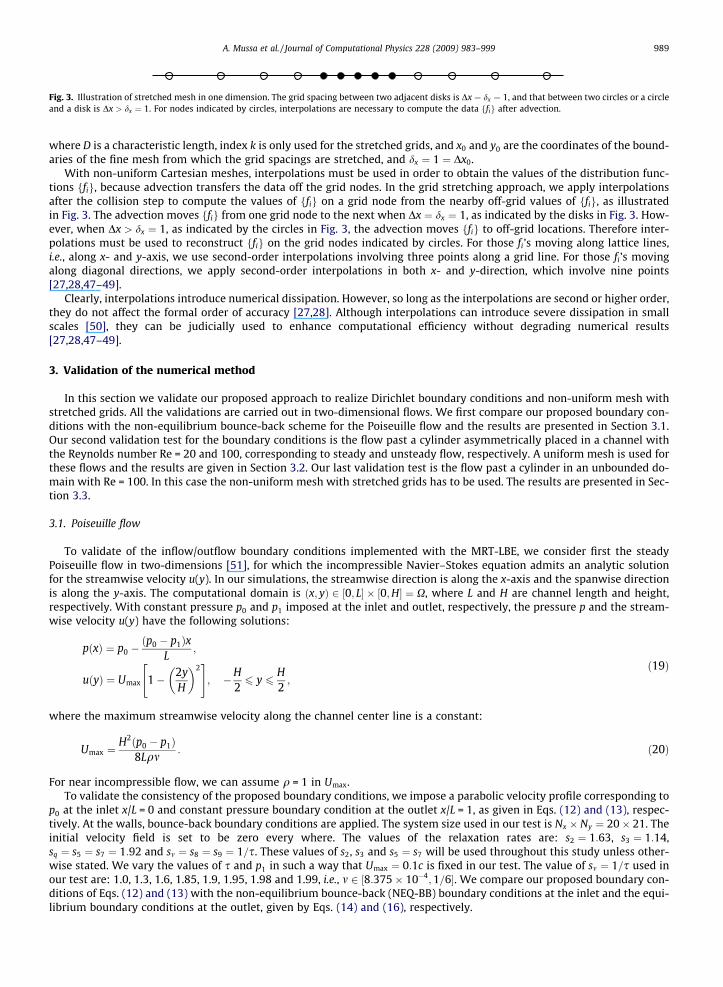
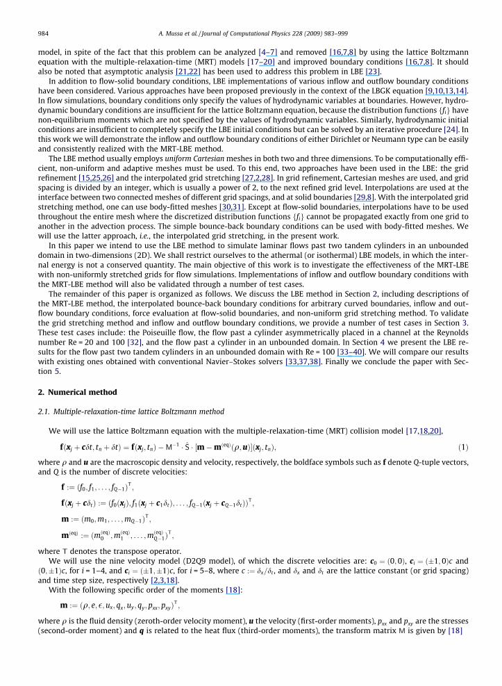
Fig. 3. Illustration of stretched mesh in one dimension. The grid spacing between two adjacent disks is Dx ¼ dx ¼ 1, and that between two circles or a circleand a disk is Dx > dx ¼ 1. For nodes indicated by circles, interpolations are necessary to compute the data ffig after advection.

A. Mussa et al. / Journal of Computational Physics 228 (2009) 983–999 989

where D is a characteristic length, index k is only used for the stretched grids, and x0 and y0 are the coordinates of the bound-aries of the fine mesh from which the grid spacings are stretched, and dx ¼ 1 ¼ Dx0.

With non-uniform Cartesian meshes, interpolations must be used in order to obtain the values of the distribution func-tions ffig, because advection transfers the data off the grid nodes. In the grid stretching approach, we apply interpolationsafter the collision step to compute the values of ffig on a grid node from the nearby off-grid values of ffig, as illustratedin Fig. 3. The advection moves ffig from one grid node to the next when Dx ¼ dx ¼ 1, as indicated by the disks in Fig. 3. How-ever, when Dx > dx ¼ 1, as indicated by the circles in Fig. 3, the advection moves ffig to off-grid locations. Therefore inter-polations must be used to reconstruct ffig on the grid nodes indicated by circles. For those fi’s moving along lattice lines,i.e., along x- and y-axis, we use second-order interpolations involving three points along a grid line. For those fi’s movingalong diagonal directions, we apply second-order interpolations in both x- and y-direction, which involve nine points[27,28,47–49].

Clearly, interpolations introduce numerical dissipation. However, so long as the interpolations are second or higher order,they do not affect the formal order of accuracy [27,28]. Although interpolations can introduce severe dissipation in smallscales [50], they can be judicially used to enhance computational efficiency without degrading numerical results[27,28,47–49].

3. Validation of the numerical method

In this section we validate our proposed approach to realize Dirichlet boundary conditions and non-uniform mesh withstretched grids. All the validations are carried out in two-dimensional flows. We first compare our proposed boundary con-ditions with the non-equilibrium bounce-back scheme for the Poiseuille flow and the results are presented in Section 3.1.Our second validation test for the boundary conditions is the flow past a cylinder asymmetrically placed in a channel withthe Reynolds number Re = 20 and 100, corresponding to steady and unsteady flow, respectively. A uniform mesh is used forthese flows and the results are given in Section 3.2. Our last validation test is the flow past a cylinder in an unbounded do-main with Re = 100. In this case the non-uniform mesh with stretched grids has to be used. The results are presented in Sec-tion 3.3.

3.1. Poiseuille flow

To validate of the inflow/outflow boundary conditions implemented with the MRT-LBE, we consider first the steadyPoiseuille flow in two-dimensions [51], for which the incompressible Navier–Stokes equation admits an analytic solutionfor the streamwise velocity u(y). In our simulations, the streamwise direction is along the x-axis and the spanwise directionis along the y-axis. The computational domain is ðx; yÞ 2 ½0; L� � ½0;H� ¼ X, where L and H are channel length and height,respectively. With constant pressure p0 and p1 imposed at the inlet and outlet, respectively, the pressure p and the stream-wise velocity u(y) have the following solutions:

pðxÞ ¼ p0 �ðp0 � p1Þx

L;

uðyÞ ¼ Umax 1� 2yH

� �2" #

; �H26 y 6

H2;

ð19Þ

where the maximum streamwise velocity along the channel center line is a constant:

Umax ¼H2ðp0 � p1Þ

8Lqm: ð20Þ

For near incompressible flow, we can assume q = 1 in Umax.To validate the consistency of the proposed boundary conditions, we impose a parabolic velocity profile corresponding to

p0 at the inlet x/L = 0 and constant pressure boundary condition at the outlet x/L = 1, as given in Eqs. (12) and (13), respec-tively. At the walls, bounce-back boundary conditions are applied. The system size used in our test is Nx � Ny ¼ 20� 21. Theinitial velocity field is set to be zero every where. The values of the relaxation rates are: s2 ¼ 1:63, s3 ¼ 1:14,sq ¼ s5 ¼ s7 ¼ 1:92 and sm ¼ s8 ¼ s9 ¼ 1=s. These values of s2, s3 and s5 ¼ s7 will be used throughout this study unless other-wise stated. We vary the values of s and p1 in such a way that Umax ¼ 0:1c is fixed in our test. The value of sm ¼ 1=s used inour test are: 1.0, 1.3, 1.6, 1.85, 1.9, 1.95, 1.98 and 1.99, i.e., m 2 ½8:375� 10�4;1=6�. We compare our proposed boundary con-ditions of Eqs. (12) and (13) with the non-equilibrium bounce-back (NEQ-BB) boundary conditions at the inlet and the equi-librium boundary conditions at the outlet, given by Eqs. (14) and (16), respectively.

990 A. Mussa et al. / Journal of Computational Physics 228 (2009) 983–999

When the system reaches steady state, attained after about 3,000 iterations for the smallest viscosity m 8:375� 10�4,we measure the velocity along the channel center and the result is shown in Fig. 4(a). Clearly, the proposed boundary con-ditions are more accurate than the non-equilibrium bounce-back boundary conditions: the velocity Umax obtained with theproposed boundary conditions varies at the 10�6 digit, while that obtained with the NEQ-BB boundary conditions is threeorder of magnitude larger, it varies at the 10�3 digit.

We next quantify the error in the measured viscosity m* in the same tests with a fixed inflow velocity profile of Umax ¼ 0:1cand varying s and p1 simultaneously to keep the flow profile intact. We measure the relative error in m:

Fig. 4.channe

dm ¼ jm� � mjm

; ð21Þ

where m is computed from Eq. (20), and m� is measured from the numerical simulations with varying s and p1. The results fordm are shown in Fig. 4(b). In the range of the relaxation rate sm ¼ 1=s 2 ½1;1:99�, the error in m in the simulations with theNEQ-BB boundary conditions is much larger than that with the proposed boundary conditions, and the difference is partic-ularly apparent when s is close to 1/2. This simple test clear shows the advantages of the proposed boundary conditions.

3.2. Flow past a cylinder in a channel

Our second test case to validate our code is the flow past a cylinder asymmetrically placed in channel in 2D [32]. This flowhas been used as a benchmark test [32], thus we can compare our results with existing data. The flow configuration is illus-trated in Fig. 5. We use an uniform mesh of size Nx � Ny for the simulations presented in this section. At the inlet, a parabolicvelocity profile with maximum velocity Umax is imposed. At the outlet, a constant pressure boundary condition correspond-ing to q1 ¼ 1 is used. At the channel walls, the bounce-back boundary conditions are applied. At the cylinder boundary, weuse the bounce-back, the first-order and second-order interpolated bounce-back boundary conditions [16,8]. The Reynoldsnumber is defined by the average inflow velocity U ¼ 2Umax=3 and the cylinder diameter D, i.e., Re ¼ UD=m ¼ 2UmaxD=3m.

At Re = 20, the flow is steady and a recirculation bubble is formed behind the cylinder. The quantities measured are thedrag coefficient CD, the lift coefficient CL, the recirculation bubble length Lr , and D�p, the pressure difference between the front

0 5 10 15 20

1

1.01

1.02

NE-BBPresent

a

1 1.2 1.4 1.6 1.8 210

-3

10-2

10-1

100

101NE-BBPresent

b

2D Poiseuille flow with different implementations of the inflow and out boundary conditions. (a) The normalized streamwise velocity along thel center Uc/Umax, with a fixed s = 1/1.85. (b) The s-dependence of the maximum relative error dm given by Eq. (21) for 1=s ¼ sm 2 ½1;1:99�.

Fig. 5. The geometric configuration for the flow past a cylinder asymmetrically placed in the channel.

Table 1Flow past a cylinder asymmetrically placed in a channel at Re = 20. The mesh-size dependence of the drag coefficient CD , the lift coefficient CL and the length ofthe recirculating zone Lr=D. BB, I and II denote the bounce-back, and the first-order and second-order interpolated bounce-back boundary conditions. Theresults of Ref. [32] are also included.

D=dx 10 20 30 40 80 NS [32]

CD BB 6.171 5.816 5.755 5.6855 5.6108 5.5700–5.5900I 5.6627 5.5741 5.5631 5.5600 5.5591II 5.6306 5.5621 5.5574 5.5573 5.5584

CL BB 0.0354 0.0223 0.0186 0.0164 0.0129 0.0104–0.0110I 0.0158 0.0123 0.0117 0.0115 0.0113II 0.0170 0.0134 0.0125 0.0116 0.0113

Lr=D BB 0.8953 0.8619 0.8629 0.8531 0.8480 0.8420–0.8520I 0.7696 0.8237 0.8322 0.8358 0.8402II 0.7728 0.8259 0.8344 0.8371 0.8402

D�p BB 6.1549 5.7454 5.7500 5.7856 5.8132 5.8600–5.8800I 5.6975 5.8305 5.7636 5.7823 5.8132II 5.7947 5.8470 5.7762 5.7836 5.8091

Fig. 6. The vorticity contours for the flow past a cylinder asymmetrically placed in the channel at Re = 20, with the resolution D=dx ¼ 80.

A. Mussa et al. / Journal of Computational Physics 228 (2009) 983–999 991

and the back of the cylinder normalized by q1U2=2. We use a number of meshes with different resolutions in terms of D=dx

and our results are summarized in Table 1.Fig. 6 shows the contours of the vorticity x at the inlet and outlet sections of the channel. The maximum value of jxj is

slightly larger than 1.0 within a very thin layer around the cylinder. Away from the cylinder, the vorticity is rather weak. Atthe four corners of the channel, the magnitude of x, jxj, is less than 2:0� 10�3 at both inlet and outlet, indicating that theproposed inlet/outlet boundary conditions do not generate spurious effects near the corners.

Fig. 7 shows the pressure coefficient Cp around the cylinder:

CpðhÞ ¼pðhÞ � p112 q1U2

max

; ð22Þ

where q1 ¼ 1, p1 ¼ 1=3, Umax ¼ 0:1c, and h = 0� is the stagnation point in front of the cylinder. In order to compute the pres-sure coefficient Cp, the pressure p(h) at the cylinder surface is extrapolated from mesh points in the flow domain. With theresolution D=dx ¼ 40, CpðhÞ computed with the bounce-back boundary conditions around the cylinder shows considerableoscillations, while the results obtained with the first- and second-order interpolations are much smoother, as expected.We also note that the results obtained by the first-order and second-order interpolations are very close to each other, i.e.,the second-order interpolations do not significantly improve the result of CpðhÞ.

At Re = 100, the flow becomes unsteady and a periodic vortex shedding takes place. Consequently both the drag and liftcoefficients are periodic functions in time. We measure the Strouhal number St, the maximum drag coefficient Cmax

D and themaximum lift coefficient Cmax

L with different grid resolutions indicated by D=dx. Our results are summarized in Table 2.It is worth noting that BB boundary conditions produce a very good result for Cmax

L at D=dx ¼ 10. This is not systematic: infact, BB shows only a first-order error convergence for D=dx > 10, while I and II interpolations show better trends. In a

0 60 120 180 240 300 360

-2

-1

0

1Bounce-BackLinearQuadratic

Fig. 7. Flow past a cylinder asymmetrically placed in a channel at Re = 20. The pressure coefficient CpðhÞ around the cylinder surface is computed with threedifferent boundary conditions. The resolution is D=dx ¼ 40. h = 0� is the stagnation point in front of cylinder.

Table 2Flow past a cylinder asymmetrically placed in a channel at Re = 100. The mesh-size dependence of the Strouhal number St, the maximum drag coefficient Cmax

D

and the maximum lift coefficient CmaxL . BB, I and II denote the bounce-back, first-order interpolation and second-order interpolation boundary conditions,

respectively.

D=dx 10 20 40 80 NS [32]

St BB 0.2778 0.2930 0.2972 0.2979 0.2950–0.3050I 0.2947 0.2991 0.2993 0.2995II 0.2953 0.3000 0.2993 0.2995

CmaxD BB 3.951 3.329 3.241 3.266 3.2200–3.2400

I 3.250 3.205 3.235 3.253II 3.200 3.198 3.250 3.256

CmaxL BB 0.974 0.844 0.922 1.007 0.9900–1.0100

I 0.566 0.913 1.006 1.030II 0.601 0.939 1.031 1.033

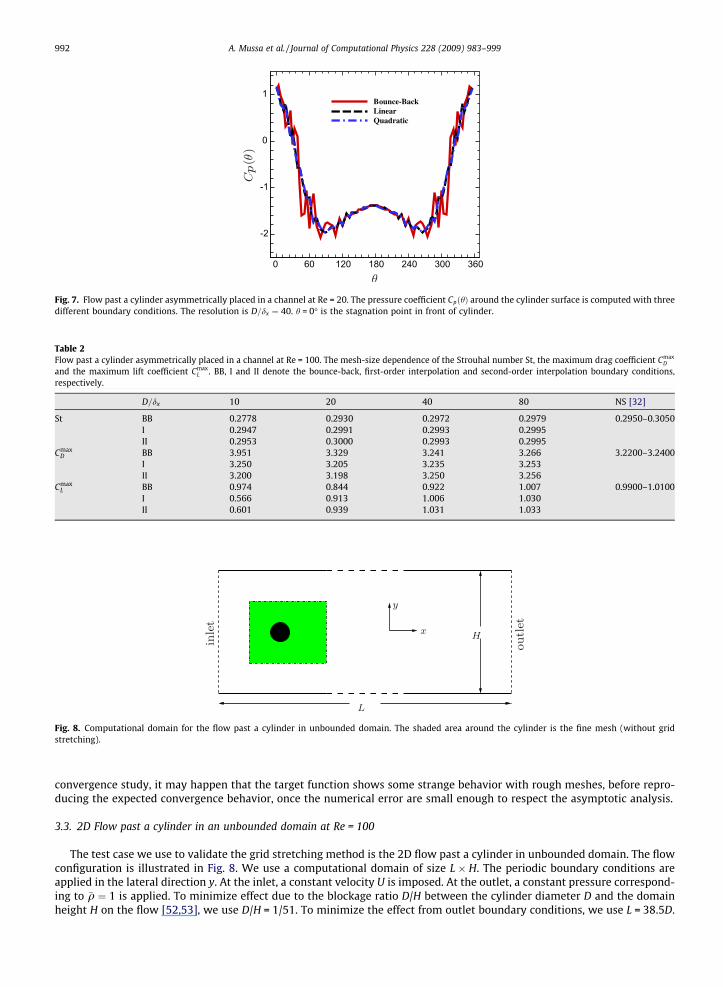
Fig. 8. Computational domain for the flow past a cylinder in unbounded domain. The shaded area around the cylinder is the fine mesh (without gridstretching).

992 A. Mussa et al. / Journal of Computational Physics 228 (2009) 983–999

convergence study, it may happen that the target function shows some strange behavior with rough meshes, before repro-ducing the expected convergence behavior, once the numerical error are small enough to respect the asymptotic analysis.

3.3. 2D Flow past a cylinder in an unbounded domain at Re = 100

The test case we use to validate the grid stretching method is the 2D flow past a cylinder in unbounded domain. The flowconfiguration is illustrated in Fig. 8. We use a computational domain of size L � H. The periodic boundary conditions areapplied in the lateral direction y. At the inlet, a constant velocity U is imposed. At the outlet, a constant pressure correspond-ing to �q ¼ 1 is applied. To minimize effect due to the blockage ratio D/H between the cylinder diameter D and the domainheight H on the flow [52,53], we use D/H = 1/51. To minimize the effect from outlet boundary conditions, we use L = 38.5D.

Table 32D Flow past a cylinder in unbounded domain at Re = 100. The dependence of the Strouhal number St, the mean drag coefficient CD and the RMS lift coefficienteCL on the size of fine mesh in downstream direction (nD) and in the lateral direction ((2m + 1)D). Beyond the fine mesh, the grid spacings are stretchedaccording to Eq. (18). The results obtained by the LBE with a uniform fine mesh for the entire domain (LBE) and by a unstructured-grid finite volume Navier–Stokes solver (NS) [38] are also given in the table.

The height of fine mesh = 3D LBE NS [38]

n 1 2 4 8 16

St 0.147 0.154 0.156 0.159 0.159 0.161 0.164CD 1.1713 1.3099 1.3142 1.3241 1.3243 1.355 1.33eCL 5:5 � 10�5 0.249 0.181 0.186 0.188 0.191 0.23

The length of fine mesh = (4 + 1 + 8)D

m 1 2 4 8 16

St 0.1587 0.1587 0.1590 0.1587 0.1587 0.161 0.164CD 1.3221 1.3224 1.3223 1.3227 1.3232 1.355 1.33eCL 0.1841 0.1848 0.1847 0.1853 0.1863 0.191 0.23

A. Mussa et al. / Journal of Computational Physics 228 (2009) 983–999 993

The cylinder center is located in the middle of the computational domain in y-direction, and 13D away from the inlet bound-ary. With a domain size of L� H ¼ 38:5D� 51D, non-uniform mesh would greatly enhance the computational efficiency.

We test the following meshes in our simulations. First, we use a fine mesh with a height of 3D and width of (4 + 1 + n) D,of which 4D portion is located upstream to the cylinder front, and nD portion is downstream to the cylinder back, as illus-trated by the shaded area around the cylinder in Fig. 8. Outside the fine mesh, grid spacing is stretched exponentially in bothdirections according to Eq. (18), with D as the cylinder diameter. We vary the downstream fraction of the fine mesh by vary-ing n to observe the effect due to the fine mesh size in streamwise direction. Similarly, we will also fix the fine mesh length at(4 + 1 + 8) D, and vary the height of the fine mesh (2m + 1) D. All the measurements are made after 100,000 iterations to en-sure that the system has reached the periodic state.

The results of the Strouhal number St, the mean drag coefficient CD and the root-mean-square (RMS) lift coefficient eCL aresummarized in Table 3, which shows the fine-mesh size dependence of St, CD and eCL by varying the fine-mesh length indownstream direction the height in lateral direction. The resolution for the fine mesh is D=dx ¼ 40. Beyond the fine mesh,the grid spacings are stretched according to Eq. (18). We also include the results obtained by the LBE with a uniform finemesh for the entire domain (LBE) and by a unstructured-grid finite volume Navier–Stokes solver (NS) [38] in Table 3. Thegrid number covered by the uniform fine mesh is ð38:5� 40Þ � ð51� 40Þ ¼ 1540� 2040 3:1� 106.

The results of Table 3 clearly show the effect of the size of the fine mesh about the cylinder. Clearly the effect of the finemesh size diminishes as the fine mesh size enlarges. The results obtained with stretched grids agree well with that obtainedwith the uniform fine mesh, so long as the size of the fine mesh covering the cylinder is sufficiently large, e.g., ð4þ 1þ 8ÞD� 5D ¼ 520� 200. However, if the size of the fine mesh is not large enough, e.g., ð4þ 1þ 1ÞD� 5D ¼ 520� 200 forn = 1, the result of eC L obtained with this mesh is rather inaccurate, as shown in Table 3. This indicates that one must providesufficient grid resolution behind the cylinder where vortex shedding takes place. With the fine mesh size fixed atð4þ 1þ 8ÞD� 5D ¼ 520� 200 for n = 8, the grid number of the entire mesh with non-uniformly stretched grids is about0:5� 106, which is only about 1/16 of the mesh size of the uniform fine grid. Therefore, the grid stretching method can sig-nificantly enhance computational efficiency. Compared to the results obtained by the Navier–Stokes solver [38], the largestdifference occurs in the RMS lift coefficient eCL, about 17%. Our results also show that the LBE method is second-order accu-rate [49].

4. Flows past two tandem cylinders at Re = 100

Our code is written in C++ with a open-source version of the Message Passing Interface library (MPICH). The numericalsimulations presented in this work were carried out on cluster computers available to us at the Department of ComputerScience, Old Dominion University (ODU) and Politecnico di Torino.

4.1. Computational domain, mesh and boundary conditions

The computational domain for flows past two tandem cylinders of equal diameter D is a rectangle of sizeL� H ¼ ð13:5þ sþ 25:5ÞD� 47D, where s is the dimensionless spacing between two cylinder centers in terms of D. The dis-tance between the inlet boundary to the first cylinder center is 13.5D, and that between the outlet boundary to the secondcylinder center is 25.5D. The cylinders are situated at the centerline of the domain, as illustrated in Fig. 9. A rectangular areaof size ð4:5þ sþ 8:5ÞD� 5D including both cylinders is covered by a uniform fine mesh, as indicated by the shade rectanglein Fig. 9. The distance between the front boundary of the fine mesh to the first cylinder center is 4.5D, and that between theback boundary of the fine mesh to the second cylinder center is 8.5D. The fine mesh has a height of 5D and it is placed

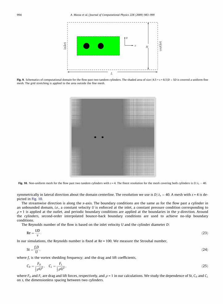
Fig. 9. Schematics of computational domain for the flow past two tandem cylinders. The shaded area of size (4.5 + s + 8.5)D � 5D is covered a uniform finemesh. The grid stretching is applied to the area outside the fine mesh.

Fig. 10. Non-uniform mesh for the flow past two tandem cylinders with s = 4. The finest resolution for the mesh covering both cylinders is D=dx ¼ 40.

994 A. Mussa et al. / Journal of Computational Physics 228 (2009) 983–999

symmetrically in lateral direction about the domain centerline. The resolution we use is D=dx ¼ 40. A mesh with s = 4 is de-picted in Fig. 10.

The streamwise direction is along the x-axis. The boundary conditions are the same as for the flow past a cylinder inan unbounded domain, i.e., a constant velocity U is enforced at the inlet, a constant pressure condition corresponding toq = 1 is applied at the outlet, and periodic boundary conditions are applied at the boundaries in the y-direction. Aroundthe cylinders, second-order interpolated bounce-back boundary conditions are used to achieve no-slip boundaryconditions.

The Reynolds number of the flow is based on the inlet velocity U and the cylinder diameter D:

Re ¼ UDm: ð23Þ

In our simulations, the Reynolds number is fixed at Re = 100. We measure the Strouhal number,

St ¼ fsDU; ð24Þ

where fs is the vortex shedding frequency; and the drag and lift coefficients,

CD ¼FD

12 qU2 ; CL ¼

FL

12 qU2 ; ð25Þ

where FD and FL are drag and lift forces, respectively, and q = 1 in our calculations. We study the dependence of St, CD and CL

on s, the dimensionless spacing between two cylinders.

A. Mussa et al. / Journal of Computational Physics 228 (2009) 983–999 995

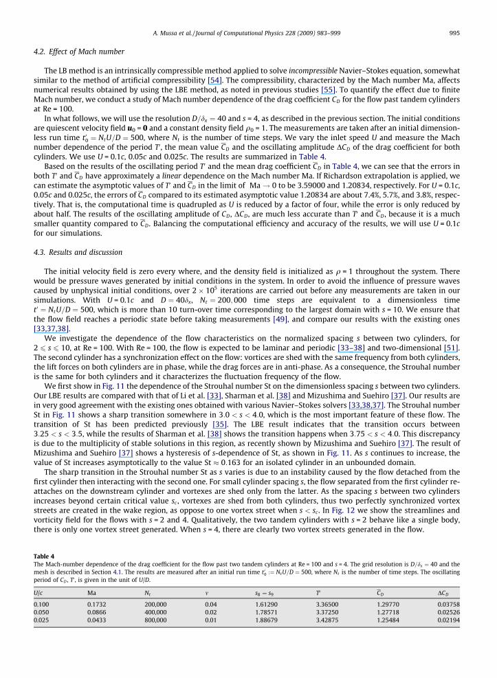
4.2. Effect of Mach number

The LB method is an intrinsically compressible method applied to solve incompressible Navier–Stokes equation, somewhatsimilar to the method of artificial compressibility [54]. The compressibility, characterized by the Mach number Ma, affectsnumerical results obtained by using the LBE method, as noted in previous studies [55]. To quantify the effect due to finiteMach number, we conduct a study of Mach number dependence of the drag coefficient CD for the flow past tandem cylindersat Re = 100.

In what follows, we will use the resolution D=dx ¼ 40 and s = 4, as described in the previous section. The initial conditionsare quiescent velocity field u0 = 0 and a constant density field q0 = 1. The measurements are taken after an initial dimension-less run time t00 ¼ NtU=D ¼ 500, where Nt is the number of time steps. We vary the inlet speed U and measure the Machnumber dependence of the period T0, the mean value CD and the oscillating amplitude DCD of the drag coefficient for bothcylinders. We use U = 0.1c, 0.05c and 0.025c. The results are summarized in Table 4.

Based on the results of the oscillating period T0 and the mean drag coefficient CD in Table 4, we can see that the errors inboth T0 and CD have approximately a linear dependence on the Mach number Ma. If Richardson extrapolation is applied, wecan estimate the asymptotic values of T0 and CD in the limit of Ma! 0 to be 3.59000 and 1.20834, respectively. For U = 0.1c,0.05c and 0.025c, the errors of CD compared to its estimated asymptotic value 1.20834 are about 7.4%, 5.7%, and 3.8%, respec-tively. That is, the computational time is quadrupled as U is reduced by a factor of four, while the error is only reduced byabout half. The results of the oscillating amplitude of CD, DCD, are much less accurate than T0 and CD, because it is a muchsmaller quantity compared to CD. Balancing the computational efficiency and accuracy of the results, we will use U = 0.1cfor our simulations.

4.3. Results and discussion

The initial velocity field is zero every where, and the density field is initialized as q = 1 throughout the system. Therewould be pressure waves generated by initial conditions in the system. In order to avoid the influence of pressure wavescaused by unphysical initial conditions, over 2� 105 iterations are carried out before any measurements are taken in oursimulations. With U = 0.1c and D ¼ 40dx, Nt ¼ 200;000 time steps are equivalent to a dimensionless timet0 ¼ NtU=D ¼ 500, which is more than 10 turn-over time corresponding to the largest domain with s = 10. We ensure thatthe flow field reaches a periodic state before taking measurements [49], and compare our results with the existing ones[33,37,38].

We investigate the dependence of the flow characteristics on the normalized spacing s between two cylinders, for2 6 s 6 10, at Re = 100. With Re = 100, the flow is expected to be laminar and periodic [33–38] and two-dimensional [51].The second cylinder has a synchronization effect on the flow: vortices are shed with the same frequency from both cylinders,the lift forces on both cylinders are in phase, while the drag forces are in anti-phase. As a consequence, the Strouhal numberis the same for both cylinders and it characterizes the fluctuation frequency of the flow.

We first show in Fig. 11 the dependence of the Strouhal number St on the dimensionless spacing s between two cylinders.Our LBE results are compared with that of Li et al. [33], Sharman et al. [38] and Mizushima and Suehiro [37]. Our results arein very good agreement with the existing ones obtained with various Navier–Stokes solvers [33,38,37]. The Strouhal numberSt in Fig. 11 shows a sharp transition somewhere in 3:0 < s < 4:0, which is the most important feature of these flow. Thetransition of St has been predicted previously [35]. The LBE result indicates that the transition occurs between3:25 < s < 3:5, while the results of Sharman et al. [38] shows the transition happens when 3:75 < s < 4:0. This discrepancyis due to the multiplicity of stable solutions in this region, as recently shown by Mizushima and Suehiro [37]. The result ofMizushima and Suehiro [37] shows a hysteresis of s-dependence of St, as shown in Fig. 11. As s continues to increase, thevalue of St increases asymptotically to the value St 0:163 for an isolated cylinder in an unbounded domain.

The sharp transition in the Strouhal number St as s varies is due to an instability caused by the flow detached from thefirst cylinder then interacting with the second one. For small cylinder spacing s, the flow separated from the first cylinder re-attaches on the downstream cylinder and vortexes are shed only from the latter. As the spacing s between two cylindersincreases beyond certain critical value sc , vortexes are shed from both cylinders, thus two perfectly synchronized vortexstreets are created in the wake region, as oppose to one vortex street when s < sc. In Fig. 12 we show the streamlines andvorticity field for the flows with s = 2 and 4. Qualitatively, the two tandem cylinders with s = 2 behave like a single body,there is only one vortex street generated. When s = 4, there are clearly two vortex streets generated in the flow.

Table 4The Mach-number dependence of the drag coefficient for the flow past two tandem cylinders at Re = 100 and s = 4. The grid resolution is D=dx ¼ 40 and themesh is described in Section 4.1. The results are measured after an initial run time t00 :¼ NtU=D ¼ 500, where Nt is the number of time steps. The oscillatingperiod of CD , T0 , is given in the unit of U/D.

U/c Ma Nt m s8 ¼ s9 T0 CD DCD

0.100 0.1732 200,000 0.04 1.61290 3.36500 1.29770 0.037580.050 0.0866 400,000 0.02 1.78571 3.37250 1.27718 0.025260.025 0.0433 800,000 0.01 1.88679 3.42875 1.25484 0.02194

0 5 100.1

0.15

LBESharmanetal.Mizushimaetal.Lietal.

Fig. 11. Flow past two tandem cylinders at Re = 100. The dependence of the Strouhal number St on the dimensionless spacing s between two cylinders. TheLBE results are compared with that of Li et al. [33], Sharman et al. [38] and Mizushima and Suehiro [37]. The dash-dot line indicates the value of St 0:164for a single cylinder in an unbounded domain at Re = 100.

Fig. 12. Flow past two tandem cylinders at Re = 100 with s = 2 (top row) and s = 4 (bottom row). Instantaneous flow fields: streamlines (left column) andvorticity contours (right column).

0 5 10

1.2

1.3

LBESharmanetal.Mizushimaetal.

a

0 5 10

0

0.5

1

LBESharmanetal.Mizushimaetal.

b

Fig. 13. Flow past two tandem cylinders at Re = 100. The dependence of the mean drag coefficient CD on the dimensionless spacing s between two cylinders.(a) CD for the upstream cylinder. The dash-dot line indicates the value of CD ¼ 1:33 for a single cylinder in an unbounded domain at Re = 100. (b) CD for thedown-stream cylinder.

996 A. Mussa et al. / Journal of Computational Physics 228 (2009) 983–999

A. Mussa et al. / Journal of Computational Physics 228 (2009) 983–999 997

Fig. 13 shows the mean drag coefficient CD for both cylinders as functions of the spacing s between two cylinders. Themean drag coefficient CD for the upstream cylinder is larger than that for the downstream one for 2 6 s 6 10. Whens > sc , the value of CD for the first cylinder increases gradually to CD 1:33 for an isolated cylinder in an unbounded domain;when s = 10, it is very close to 1.33. For the second cylinder, the value of CD is much smaller than that of the first, indicatingthat the suction force due to the first cylinder is rather strong. When s < sc , CD for the first cylinder is much smaller than thesingle-cylinder value CD 1:33, and CD for the second cylinder is even negative, due to strong suction force induced by thefirst cylinder. Again, a sharp transition in CD occurs at s ¼ sc .

Figs. 14 and 15 show the root-mean-square (RMS) values of the drag and lift coefficients, eCD and eCL, respectively, com-pared with the results of Sharman et al. [38]. The values of eCD and eCL all show a sharp increase at s ¼ sc . When s < sc , both eCD

and eCL for the first cylinder are considerably smaller than their corresponding values for a single cylinder in an unboundeddomain. Soon after the transition occurs, both eCD and eCL exceed their corresponding values for a single cylinder and reachtheir maxima at s 4:0, then gradually decrease to their respective single-cylinder values. Both eCD and eCL for the secondcylinder behave very similar to that for the first one, i.e., they both encounter a drastic increase at s ¼ sc , reach their maximaat s 4:0, then gradually decrease to their respective asymptotic values, which should presumably be that for a single cyl-inder in an unbounded domain as s!1.

Our results shown in Figs. 11, 13–15 quantitatively agree well with the existing results [33,37,38]. All the global flowfeatures are quantitatively captured by the LBE simulations. We also notice that there are discrepancies between our resultsand the ones obtained by various Navier–Stokes solvers [37,38]. Compared to the results of Mizushima and Suehiro [37], our

0 5 10

0

0.01

0.02

LBESharmanetal.

a

0 5 10

0

0.05

0.1

0.15

LBESharmanetal.

b

Fig. 14. Flow past two tandem cylinders at Re = 100. The dependence of the RMS drag coefficient eCD on the dimensionless spacing s between two cylinders.(a) eCD for the upstream cylinder. The dash-dot line indicates the value of eCD 0:0063 for a single cylinder in an unbounded domain. (b) eC D for the down-stream cylinder.

0 5 100

0.1

0.2

0.3

LBESharmanetal.

a

0 5 100

0.5

1

LBESharmanetal.

b

Fig. 15. Flow past two tandem cylinders at Re = 100. The dependence of the RMS lift coefficient eC L on the dimensionless spacing s between two cylinders.(a) eCL for the upstream cylinder. The dash-dot line indicates the value of eC L 0:23 for a single cylinder in an unbounded domain. (b) eCL for the down-stream cylinder.

998 A. Mussa et al. / Journal of Computational Physics 228 (2009) 983–999

results agree better with that of Sharman et al. [38]. Besides the fundamental difference in the solution techniques, we notethat body-fitted meshes were used by Sharman et al. [38], and the Cartesian meshes are used in the present work. Also, thediscrepancy between our results and that of Sharman et al. [38] may be due to the multiplicity of the solutions near the crit-ical spacing sc , as indicated in Figs. 11 and 13.

5. Conclusions

In this paper we use the lattice Boltzmann equation with multiple-relaxation-time collision model to simulate laminarflows in two dimensions. For the no-slip boundary conditions at flow-solid boundaries, we apply the interpolatedbounce-back boundary conditions [29,8]. For the inflow and outflow boundary conditions, we use a general bounce-backboundary conditions which can be easily, naturally and consistently realized with the MRT-LBE in particular. To enhancethe computational efficiency of the LBE method with uniform meshes, we use the grid stretching method to deal with thenon-uniform Cartesian mesh. Even though the techniques we use in this work are simple and thus easy to implement,the numerical results demonstrate their effectiveness.

The MRT-LBE with non-uniformly stretched Cartesian mesh has been validated by using a number of test cases, includingthe Poiseuille flow, the flow past a cylinder asymmetrically placed in a channel, and the flow past a cylinder in an unboundeddomain. The validated code is used to simulate flows past two tandem cylinders in an unbounded domain at Re = 100 withthe dimensionless spacing between the cylinders 2 6 s 6 10. Our results agree well quantitatively with the existing ones ob-tained by using the Navier–Stokes solvers.

Acknowledgements

The authors are grateful to Dr. Meelan M. Choudhari of NASA Langley Research Center for suggesting this problem to themand for his insightful comments of this work, Prof. Manfred Krafczyk for bringing our attention the effects of the Mach-numberon the results obtained by the LBE method, and Dr. Th. Zeiser for his careful reading of our paper and his critical comments.A.M. would like to thank Politecnico di Torino for financial support, and the Department of Mathematics & Statistics and Cen-ter for Computational Sciences at Old Dominion University (ODU) for sponsoring his visit to ODU, between March to July,2006, during which significant part of this work was accomplished. A.M. would also like to thank Prof. Michele Calì and Prof.Romano Borchiellini of Politecnico di Torino for their support and encouragement of this work. The results reported in thispaper are a part of the Master’s thesis of A.M. [49]. L.S.L would like to acknowledge the support from the National ScienceFoundation of the US through the Grant CBET-0500213.

References

[1] D. Yu, R. Mei, L.-S. Luo, W. Shyy, Viscous flow computations with the method of lattice Boltzmann equation, Prog. Aerospace Sci. 39 (2003) 329–367.[2] X. He, L.-S. Luo, A priori derivation of the lattice Boltzmann equation, Phys. Rev. E 55 (1997) R6333–R6336.[3] X. He, L.-S. Luo, Theory of lattice Boltzmann method: from the Boltzmann equation to the lattice Boltzmann equation, Phys. Rev. E 56 (1997) 6811–

6817.[4] I. Ginzbourg, Boundary conditions problems in lattice gas methods for single and multiple phases, PhD thesis, Universite Paris VI, France, 1994.[5] I. Ginzbourg, P.M. Adler, Boundary flow condition analysis for the three-dimensional lattice Boltzmann model, J. Phys. II 4 (1994) 191–214.[6] I. Ginzburg, D. d’Humières, Local second-order boundary methods for lattice Boltzmann models, J. Stat. Phys. 84 (1996) 927–971.[7] I. Ginzburg, D. d’Humières, Multireflection boundary conditions for lattice Boltzmann models, Phys. Rev. E 68 (2003) 066614.[8] C. Pan, L.-S. Luo, C.T. Miller, An evaluation of lattice Boltzmann schemes for porous medium flow simulation, Comput. Fluids 35 (8/9) (2006) 898–909.[9] D.W. Grunau, Lattice Methods for Modeling of Hydrodynamics, PhD Thesis, Colorado State University, Fort Colins, USA, 1993.

[10] P.A. Skordos, Initial and boundary conditions for the lattice Boltzmann method, Phys. Rev. E 48 (1993) 4823.[11] T. Inamuro, M. Yoshino, F. Ogino, A non-slip boundary condition for lattice Boltzmann simulations, Phys. Fluids 7 (1996) 2928.[12] R.S. Maier, R.S. Bernard, D.W. Grunau, Boundary conditions for the lattice Boltzmann method, Phys. Fluids 8 (1996) 1788.[13] S. Chen, D.O. Martìnez, R. Mei, On boundary conditions in lattice Boltzmann methods, Phys. Fluids 8 (1996) 2527.[14] Q. Zou, X. He, On pressure and velocity boundary conditions for the lattice Boltzmann BGK model, Phys. Fluids 9 (6) (1997) 1591–1598.[15] O. Filippova, D. Hänel, Grid refinement for lattice-BGK models, J. Comput. Phys. 147 (1) (1998) 219–228.[16] M. Bouzidi, M. Firdaouss, P. Lallemand, Momentum transfer of Boltzmann-lattice fluid with boundaries, Phys. Fluids 13 (2001) 3452–3459.[17] D. d’Humières, Generalized lattice-Boltzmann equations, in: B.D. Shizgal, D.P. Weave (Eds.), Rarefied Gas Dynamics: Theory and Simulations, Progress

in Astronautics and Aeronautics, vol. 159, American Institute of Aeronautics and Astronautics (AIAA), Washington, DC, USA, 1992, pp. 450–458. AIAA.[18] P. Lallemand, L.-S. Luo, Theory of the lattice Boltzmann method: dispersion, dissipation, isotropy, Galilean invariance, and stability, Phys. Rev. E 61

(2000) 6546–6562.[19] D. d’Humières, M. Bouzidi, P. Lallemand, Thirteen-velocity three-dimensional lattice Boltzmann model, Phys. Rev. E 63 (2001) 066702.[20] D. d’Humières, I. Ginzburg, M. Krafczyk, P. Lallemand, L.-S. Luo, Multiple-relaxation-time lattice Boltzmann models in three-dimensions, Philos. Trans.

Roy. Soc. Lond. A 360 (2002) 437–451.[21] M. Junk, W.-A. Yong, Rigorous Navier–Stokes limit of the lattice Boltzmann equation, Asymptotic Anal. 35 (2003) 165–185.[22] M. Junk, A. Klar, L.-S. Luo, Asymptotic analysis of the lattice Boltzmann equation, J. Comput. Phys. 210 (2) (2005) 676–704.[23] M. Junk, Z. Yang, Analysis of the lattice Boltzmann boundary conditions, Proc. Appl. Math. Mech. 3 (2003) 76–79.[24] R. Mei, L.-S. Luo, P. Lallemand, D. d’Humières, Consistent initial conditions for lattice Boltzmann simulations, Comput. Fluids 35 (8/9) (2006) 855–862.[25] B. Crouse, E. Rank, M. Krafczyk, J. Tölke, A LB-based approach for adaptive flow simulations, Int. J. Mod. Phys. B 17 (2003) 109–112.[26] J. Tölke, S. Freudiger, M. Krafczyk, An adaptive scheme using hierarchical grids for lattice Boltzmann multi-phase flow simulations, Comput. Fluids 35

(8/9) (2006) 820–830.[27] X. He, L.-S. Luo, M. Dembo, Some progress in lattice Boltzmann method: Part I. Nonuniform mesh grids, J. Comput. Phys. 129 (1996) 357–363.[28] X. He, L.-S. Luo, M. Dembo, Some progress in lattice Boltzmann method: enhancement of Reynolds number in simulations, Physica A 239 (1997) 276–

285.

A. Mussa et al. / Journal of Computational Physics 228 (2009) 983–999 999

[29] M. Bouzidi, D. d’Humières, P. Lallemand, L.-S. Luo, Lattice Boltzmann equation on a two-dimensional rectangular grid, J. Comput. Phys. 172 (2001) 704–717.

[30] X. He, G.D. Doolen, Lattice Boltzmann method on curvilinear coordinates systems: flow around a circular cylinder, J. Comput. Phys. 134 (1997) 306–315.

[31] X. He, G.D. Doolen, Lattice Boltzmann method on a curvilinear coordinate system: vortex shedding behind a circular cylinder, Phys. Rev. E 56 (1)(1997).

[32] M. Schäfer, S. Turek, Benchmark computations of laminar flow around a cylinder, in: E.H. Hirschel (Ed.), Flow simulation with high-performancecomputation II, Notes on Numerical Fluid Mechanics, vol. 52, Vieweg Verlag, Braunschweig, Germany, 1996, pp. 547–566.

[33] J. Li, A. Chambarel, M. Donneaud, R. Martin, Numerical study of laminar flow past one and two circular cylinders, Comput. Fluids 19 (2) (1991) 155–170.

[34] M.M. Zdravkovich, Flow Around Circular Cylinders. Volume 2: Applications, Oxford Science Publication, Oxford, 2003.[35] S. Mittal, V. Kumar, A. Raghuvanshi, Unsteady incompressible flows past two cylinders in tandem and staggered arrangements, Int. J. Numer. Meth.

Fluids 25 (1997) 1315–1344.[36] J.R. Meneghini, F. Saltara, C.L.R. Siqueira, J.A. Ferrari, Numerical simulation of the flow interference between two circular cylinders in tandem and side

by side arrangements, J. Fluid Struct. 15 (2001) 327–350.[37] J. Mizushima, N. Suehiro, Instability and transition of flow past two tandem circular cylinders, Phys. Fluids 17 (10) (2005) 104107.[38] B. Sharman, F.S. Lien, L. Davidson, C. Norberg, Numerical predictions of low Reynolds number flows over two tandem circular cylinder, Int. J. Numer.

Meth. Fluids 47 (2005) 423–447.[39] L.N. Jenkins, D.H. Neuhart, C.B. McGinley, M.M. Choudhari, M.R. Khorrami, Measurements of Unsteady Wake Interference between Tandem Cylinders,

AIAA Paper 2006-3202, 2006.[40] D.P. Lockard, M.R. Khorrami, M.M. Choudhari, F.V. Hutcheson, T.F. Brooks, Tandem Cylinder Noise Predictions, AIAA Paper 2007-3450, 2007.[41] X. He, L.-S. Luo, Lattice Boltzmann model for the incompressible Navier–Stokes equation, J. Stat. Phys. 88 (1997) 927–944.[42] L.-S. Luo, Comment on discrete Boltzmann equation for microfluidics, Phys. Rev. Lett. 92 (13) (2004) 139401.[43] R. Mei, D. Yu, W. Shyy, L.-S. Luo, Force evaluation in the lattice Boltzmann method involving curved geometry, Phys. Rev. E 65 (2002) 041203.[44] M. Cheng, Q. Yao, L.-S. Luo, Simulation of flow past a rotating circular cylinder near a plane wall, Int. J. Comput. Fluid Dyn. 20 (6) (2006) 391–400.[45] M. Cheng, L.-S. Luo, Characteristics of two-dimensional flow around a rotating circular near a plane wall, Phys. Fluids 19 (6) (2007) 063601.[46] A.J.C. Ladd, Numerical simulations of particulate suspensions via a discretized Boltzmann equation. Part 2. Numerical results, J. Fluid Mech. 271 (1994)

311–339.[47] Y. Peng, L.-S. Luo, A comparative study of immersed-boundary and interpolated bounce-back methods in LBE, Prog. Comput. Fluid Dyn. 8 (1–4) (2008)

156–167.[48] H.N. Dixit, V. Babu, Simulation of high Rayleigh number natural convection in a square cavity using the lattice Boltzmann method, Int. J. Heat Mass

Trans. 49 (3/4) (2006) 727–739.[49] A. Mussa, Numerical Simulations of the Fluid flow through Tandem Cylinders by Multiple-relaxation-time Lattice Boltzmann Method, Master’s Thesis,

Politecnico di Torino, Turin, Italy, 2006.[50] P. Lallemand, L.-S. Luo, Theory of the lattice Boltzmann method: acoustic and thermal properties in two and three dimensions, Phys. Rev. E 68 (2003)

036706.[51] D.J. Tritton, Physical Fluid Dynamics, Oxford Science Publications, Oxford, 1988.[52] M. Behr, D. Hastreiter, S. Mittal, T.E. Tezduyar, Incompressible flow past a circular cylinder: dependence of the computed flow field on the location of

the lateral boundaries, Comput. Meth. Appl. Mech. Eng. 123 (1994) 309–316.[53] B. Kumar, S. Mittal, Effect of blockage on critical parameters for flow past a circular cylinder, Int. J. Numer. Meth. Fluids 50 (9) (2006) 987–1001.[54] A.J. Chorin, A numerical method for solving incompressible viscous problems, J. Comput. Phys. 2 (1) (1967) 12–26.[55] S. Geller, M. Krafczyk, J. Tölke, S. Turek, J. Hron, Benchmark computations based on lattice-Boltzmann, finite element and finite volume methods for

laminar flows, Comput. Fluids 35 (8/9) (2006) 888–897.