
Empirical Investigation Of The Laminar Thermal Entrance ...
120
University of North Dakota UND Scholarly Commons eses and Dissertations eses, Dissertations, and Senior Projects January 2015 Empirical Investigation Of e Laminar ermal Entrance Region And Turbulent Flow Heat Transfer For Non-Newtonian Silica Nanofluid In Hexagonal Tubes Emeke Kevin Opute Follow this and additional works at: hps://commons.und.edu/theses is esis is brought to you for free and open access by the eses, Dissertations, and Senior Projects at UND Scholarly Commons. It has been accepted for inclusion in eses and Dissertations by an authorized administrator of UND Scholarly Commons. For more information, please contact [email protected]. Recommended Citation Opute, Emeke Kevin, "Empirical Investigation Of e Laminar ermal Entrance Region And Turbulent Flow Heat Transfer For Non-Newtonian Silica Nanofluid In Hexagonal Tubes" (2015). eses and Dissertations. 1818. hps://commons.und.edu/theses/1818
-
Upload
khangminh22 -
Category
Documents
-
view
0 -
download
0
Transcript of Empirical Investigation Of The Laminar Thermal Entrance ...
University of North DakotaUND Scholarly Commons
Theses and Dissertations Theses, Dissertations, and Senior Projects
January 2015
Empirical Investigation Of The Laminar ThermalEntrance Region And Turbulent Flow HeatTransfer For Non-Newtonian Silica Nanofluid InHexagonal TubesEmeke Kevin Opute
Follow this and additional works at: https://commons.und.edu/theses
This Thesis is brought to you for free and open access by the Theses, Dissertations, and Senior Projects at UND Scholarly Commons. It has beenaccepted for inclusion in Theses and Dissertations by an authorized administrator of UND Scholarly Commons. For more information, please [email protected].
Recommended CitationOpute, Emeke Kevin, "Empirical Investigation Of The Laminar Thermal Entrance Region And Turbulent Flow Heat Transfer ForNon-Newtonian Silica Nanofluid In Hexagonal Tubes" (2015). Theses and Dissertations. 1818.https://commons.und.edu/theses/1818
EMPIRICAL INVESTIGATION OF THE LAMINAR THERMAL ENTRANCE
REGION AND TURBULENT FLOW HEAT TRANSFER FOR NON-NEWTONIAN
SILICA NANOFLUID IN HEXAGONAL TUBES
by
Emeke K. Opute
Bachelor of Engineering, Nnamdi Azikiwe University, 2008
A Thesis
Submitted to the Graduate Faculty
of the
University of North Dakota
In partial fulfilment of the requirements
for the degree of
Master of Science
Grand Forks, North Dakota, USA
August
2015

ii
iii
PERMISSION
Title Empirical Investigation of the Laminar Thermal Entrance Region
and Turbulent Flow Heat Transfer for Non-Newtonian Silica
Nanofluid in Hexagonal Tubes
Department Mechanical Engineering
Degree Master of Science
In presenting this thesis in partial fulfillment of the requirements for a graduate
degree from the University of North Dakota, I agree that the library of this University shall
make it freely available for inspection. I further agree that permission for extensive copying
for scholarly purposes may be granted by the professor who supervised my thesis work or,
in his absence, by the Chairperson of the department or the dean of the School of Graduate
Studies. It is understood that any copying or publication or other use of this thesis or part
thereof for financial gain shall not be allowed without my written permission. It is also
understood that due recognition shall be given to me and to the University of North Dakota
in any scholarly use which may be made of any material in my thesis.
Emeke K Opute
August 07, 2015
iv
TABLE OF CONTENTS
LIST OF FIGURES……………………………………………………………………...vii
LIST OF TABLES………………………………………………………………………..xi
NOMENCLATURE……………………………………………………………………..xii
ACKNOWLEDGEMENTS……………………………………………………………xviii
ABSTRACT…………………………………………………………………………….xix
CHAPTER
I. INTRODUCTION……………………………………………………………………..1
1.1 Research Objectives.….……………………………………………………….6
1.2 Nanofluid Applications…………...……………………….…………………..7
1.3 Study Outline……………..…………………………………………………...9
II. LITERATURE REVIEW……………………………………………………………10
2.1 Synthesis and Characterization of Nanofluids……………………………….10
Synthesis and Stability…………………………………………………...10
Characterization and Modeling…………………………………………..12
2.2 Nanofluid Viscosity, Pressure Drop and Rheology………………………….16
v
2.3 Nanofluid Heat Transfer……………………………………………………..20
2.3.1 Thermal Conductivity……………………………………………...21
2.3.2 Convective Heat Transfer………………………………………….25
III. EXPERIMENTAL APPROACH…………………………………………………...33
3.1 Description and Preparation of Nanofluid…………………………………...33
3.2 Description of Test Loop and Test Sections…………………………………34
3.3 Temperature and Heat Transfer Considerations…………………………......41
3.4 Transport Considerations…………………………………………………….42
Specific Heat and Viscosity……………………………………………...42
Non-Newtonian Fluids…………………………………………………...43
3.5 Instrument Calibration and Experimental Procedure………………………...45
3.5.1 Pressure Transducer Calibration…………………………………...45
3.5.2 Pressure Drop Measurement……………………………………….46
3.5.3 Heat Transfer Measurements………………………………………47
3.6 Validation of Experimental Method……………………...………………….47
3.7 Data Processing……………………………………..……………………….52
IV. EXPERIMENTAL RESULTS……………………………………………………..54
4.1 Water Results………………………………………………………………...55
vi
4.1.1 Friction coefficient…………………………………………………55
4.1.2. Heat transfer……………………………………………………….60
4.2. Nanofluid (9.8% vol. SiO2-Water Colloid) Results…………………………65
4.2.1 Friction coefficient…………………………………………………65
4.2.2. Local surface temperature profile for nanofluid flow……………..69
4.2.3. Heat transfer……………………………………………………….71
4.3. Nanofluid vs Water Friction Coefficient……………………………………77
4.4. Nanofluid vs water heat transfer…………………………………………….81
4.5. Pressure drop of Nanofluid versus Water…………………………………...83
V. CONCLUSIONS AND RECOMMENDATIONS………………………………….85
5.1. CONCLUSIONS……………………………………………………………85
5.2. RECOMMENDATIONS AND FUTURE WORK…………………………87
APPENDICES…………………………………………………………………………...90
A. Viscosity of Nanofluid (Sharif, 2015)……………………………………………90
B. Error Analysis…………………………………………………………………….91
Apparent Viscosity, Reynolds Number and Friction Factors Uncertainty………91
REFERENCES…………………………………………………………………………..93
vii
LIST OF FIGURES
Figure Page
1. Tube velocity boundary layer development (Çengel and Ghajar, 2011)…...….…4
2. (a) Shear stress vs Shear strain rate for various nanofluids with different
volume concentration of Al2O3 nanoparticles. (b) Yield stress as
a function of vol. % in the nanofluid. Line is the fitted
power–law equation: τy = (0.50063)ϕ1.3694 (Kole and Dey 2010)…………….19
3. Experimental Nusselt number for Al2O3/water and CuO/water nanofluids
(Heris and Etemad et al, 2006)…………………………………………………..26
4. Experimental set ups (a) for measuring pressure drop across test section
and (b) apparatus for measuring thermal conductivity of nanofluid
(Duangthongsuk & Wongwises, 2010)………………………………………….28
5. Schematic diagram of the closed loop convective laminar flow system
(Azizian, Doroodchi et al, 2014)…………………………………………………31
6. Schematic of experimental loop or setup…………………..…………………….35
7. Pressure tubes-transducer connection……………………………………………36
8. Pressure transmitter in-use position……………………………………………...38
9. Agilent Data Acquisition unit……………………………………………………38
10. External view of test section with D = 3.26 mm………………………………...39
11. Bead welding machine…………………………………………………………...40
12. Velocity gradient formed between two parallel plates…………………………..44
viii
13. Comparison of friction factor for distilled water flow in unheated
test sections D = 1.67 mm, D = 2.46 mm and D = 3.26 mm……………...……..56
14. Comparison of friction factor for distilled water flow in heated
test sections D = 1.67 mm, D = 2.46 mm and D = 3.26 mm…………………….57
15. Comparison of friction factor for heated vs unheated flow of distilled
water flow in test section D = 1.67 mm………………………………………….58
16. Comparison of friction factor for heated vs unheated flow of distilled
water flow in test section D = 2.46 mm………………………………………….58
17. Comparison of friction factor for heated vs unheated flow of distilled
water flow in test section D = 3.26 mm………………………………………….59
18. Comparison of measured Nusselt number vs Reynolds number for distilled
water flow through heated test sections………………………………………….60
19. Measured Laminar flow Nusselt number vs x+ for distilled water flow in
heated test section D = 2.46 mm compared with the Lienhard and Lienhard
(2013) correlation. Dotted lines represent ±20% error limits…………………....61
20. Comparison of Measured Nusselt number vs Gnielinski (1976) for distilled
water flow in heated test section D = 2.46 mm. Broken lines represent
error limits of ±20%...............................................................................................62
21. Measured Laminar flow Nusselt number vs x+ for distilled water flow in heated
test section D = 1.67 mm compared with the Lienhard and Lienhard (2013)
correlation. Dotted lines represent error limits of ±30%.......................................63
22. Comparison of Measured Nusselt number vs Gnielinski (1976) for distilled
water flow in heated test section D = 1.67 mm. Broken lines represent
error limits of ±10%...............................................................................................63
23. Measured Laminar flow Nusselt number vs x+ for distilled water flow in heated
test section D = 3.26 mm compared with the Lienhard and Lienhard (2013)
correlation. Dotted lines represent error limits of ±20%.......................................64
24. Comparison of Measured Nusselt number vs Gnielinski (1976) for distilled
water flow in heated test sections D = 3.26 mm. Broken lines
represent error limits of ±20%...............................................................................64
ix
25. Comparison of friction factor for nanofluid flow in unheated test sections
D = 1.67 mm, D = 2.46 mm and D = 3.26 mm……………………………...…...65
26. Comparison of friction factor for nanofluid flow in heated test sections
D = 1.67 mm, D = 2.46 mm and D = 3.26 mm…………………………………..66
27. Comparison of friction factor for heated vs unheated flow of nanofluid
flow in test section D = 1.67 mm………………………………………………...67
28. Comparison of friction factor for heated vs unheated flow of nanofluid
flow in test section D = 2.46 mm………………………………………………...67
29. Comparison of friction factor for heated vs unheated flow of nanofluid
flow in test section D = 3.26 mm………………………………………………...68
30. Surface temperature profile for nanofluid flow in test section D = 1.67 mm……69
31. Surface temperature profile for nanofluid flow in test section D = 2.46 mm……70
32. Surface temperature profile for nanofluid flow in test section D = 3.26 ..………70
33. Measured Nusselt vs Reynolds number for nanofluid flow in tubes…………….71
34. Measured Laminar flow Nusselt number vs x+ for nanofluid flow in heated
test section D = 1.67 mm compared with the Lienhard and Lienhard (2013)
correlation. Dotted lines represent error limits of ±30%.......................................72
35. Comparison of Measured Nusselt number vs Gnielinski (1976) for nanofluid
flow in heated test section D = 1.67 mm. Broken lines represent
error limits of ±30%...............................................................................................72
36. Measured Laminar flow Nusselt number vs x+ for nanofluid flow in heated
test section D = 2.46 mm compared with the Lienhard and Lienhard (2013)
correlation. Dotted lines represent error limits of ±30%.......................................73
37. Comparison of Measured Nusselt number vs Gnielinski (1976) for
nanofluid flow in heated test section D = 2.46 mm.
Broken lines represent error limits of ±30%..........................................................73
38. Measured Laminar flow Nusselt number vs x+ for nanofluid flow in heated
test section D = 3.26 mm compared with the Lienhard and Lienhard (2013)
x
correlation. Dotted lines represent error limits of ±30%.......................................74
39. Comparison of Measured Nusselt number vs Gnielinski (1976) for nanofluid
flow in heated test section D = 3.26 mm. Broken lines represent
error limits of ±20%...............................................................................................74
40. Friction coefficient compared for unheated water and unheated nanofluid
flow in the test section D = 1.67mm……………………………………………..77
41. Friction coefficient compared for unheated water and unheated nanofluid
flow in the test section D = 2.46 mm…………………………………………….78
42. Friction coefficient compared for unheated water and unheated nanofluid
flow in the test section D = 3.26 mm…………………………………………….78
43. Friction coefficient compared for heated water and heated nanofluid
flow in test section D = 1.67 mm………………………………………………...79
44. Friction coefficient compared for heated water and heated nanofluid in
test section D = 2.46 mm………………………………………………………...80
45. Friction coefficient compared for heated water and heated nanofluid in
test section D = 3.26 mm………………………………………………………...80
46. Comparison of nanofluid and water heat transfer for test section D = 1.67 mm..81
47. Comparison of nanofluid and water heat transfer for test section D= 2.46 mm…82
48. Comparison of nanofluid and water heat transfer for test section D = 3.26 mm..82
49. Comparison of pressure drop across test section D = 2.46 mm
with respect to Reynolds number………………………………………………...83
50. Comparison of pressure drop across test section D = 1.67 mm
with respect to Reynolds number………………………………………………..84
51. Comparison of pressure drop across test section D = 3.26 mm
with respect to Reynolds number………………………………………………...84
52. Change of shear stress with shear rate at different temperatures
for Silica nanoparticle colloidal suspension (9.58% by volume) Sharif (2015)…90
xi
LIST OF TABLES
Table Page
1. Friction correlations reported in the literature for nanofluid in a tube.
(Sundar and Singh, 2013) …..…………………………………………………..17
2. Nusselt number correlations reported in the literature for nanofluid in a
tube (Sundar and Singh, 2013)………………….…….……………………...…..30
3. Components of experimental setup……………………………………………....37
4. Location of thermocouple on test section surface………………………………..40
xii
NOMENCLATURE
English Letter Symbols
As Test section flow surface area [m2]
Br Ratio of nanolayer to thickness to original particle radius
C* Experimentally determined constant
Cf Equivalent Fanning Friction factor or coefficient
Cnf Specific heat of nanofluid [J/kg K]
Cnp Specific heat of nanoparticle [J/kg K]
Cbf Specific heat of basefluid [J/kg K]
D Hydraulic diameter of test section [m]
DB Brownian diffusion coefficient [m2/s]
dp Nanoparticle diameter [m]
du/dr Strain on fluid by wall [1/s]
DT Thermal diffusion coefficient [m2/s]
f Darcy friction factor
F Parallel force to liquid column [N]
xiii
f" Second derivative of dimensionless velocity
gc Conversion factor [ft lb/s2 lbf]
Jnp,B nanoparticle mass flux due to Brownian diffusion [kg/m2 s]
Jnp,T nanoparticle mass flux to thermophoresis [kg/m2 s]
K' Apparent viscosity [Pa.s]
k2 Thermal conductivity of particle [W/m K]
kB Boltzmannn constant [J/K]
kbf Thermal conductivity of basefluid [W/m K]
keff Effective thermal conductivity [W/m K]
kl Thermal conductivity of liqid [W/m K]
knf Thermal conductivity of nanofluid [W/m K]
knp Nanoparticle thermal conductivity [W/m K]
kpe Equivalent thermal conductivity of equivalent particles [W/m K]
L Length of test section [m]
ṁ Average bulk fluid mass flow rate [kg/s]
n' Degree to which fluid is non-Newtonian
NRe Reynolds number based on Reed, Metzner (1955)
Nu Nusselt Number
xiv
NuD Nusselt Number based on hydraulic diameter
Nux Average Nusselt number at axial location x
P Pressure [Pa]
Pe Peclet number
Pr Prandtl number
qs Heat flux through tube wall [W/m2]
r Equals D/2 [m]
R Equals (D/2 + t) [m]
Re Reynolds number
ReD Reynolds number based on hydraulic diameter
T Nanofluid temperature [K]
t Test section/tube thickness [m]
Tbx Fluid bulk temperature at x location [K]
Te Fluid test section's exit temperature [K]
Ti Fluid test section's inlet temperature [K]
Tm Fluid mean temperature
Twi Inner wall temperature of test section [K]
Two Outer wall temperature of test section [K]
xv
u Velocity of plate [m/s]
V Velocity of fluid flowing through test section [m/s]
Vnf Volume of nanofluid [m3]
VT Thermophoretic velocity [m/s]
x Axial location along test section or tube [m]
x+ Dimensionless axial location
y Boundary layer thickness [m]
Greek Symbols
β Thermophoretic coefficient
∂u/∂y Velocity gradient [1/s]
ΔP Pressure drop between inlet and exit of test section [Pa]
θ" Second derivative of dimensionless temperature
μ Viscosity [Pa.s]
μl Viscosity of liquid [Pa.s]
μs Viscosity of solid (spehere) particles [Pa.s]
ρ Nanofluid density [kg/m3]
ρnp Nanoparticle density [kg/m3]
τ Shear stress [Pa]

xvi
τw Shear stress at the wall of test section due to fluid flow [Pa]
ϕ Volume fraction of solid spheres or nanoparticles
φnp Mass fraction of nanoparticles
Subscript
B Brownian motion
b Bulk
bf Base fluid
D Hydraulic diameter
e Exit
i Inlet
l Liquid
nf Nanofluid
np Nanoparticle
r Ratio
s Surface
T Thermal or Thermophoretic
w Wall
wi Inner wall

xvii
wo Outer wall
x Axial location
Superscript
" Second derivative
+ Dimensionless

xviii
ACKNOWLEDGEMENTS
I am grateful for the opportunities, excellent research facilities and funding that I received
from the University of North Dakota in the course of my studies here, all of which have
led me to my developing this thesis. I thank my advisor Dr. Clement Tang and the other
members of my committee, Dr. Gautham Krishnamoorthy and Dr. Nanak Grewal for their
exquisite mentoring, their efforts were invaluable to the execution of this project. Finally,
I thank my family, who have loved, provided for and strongly supported me all my life.

xix
ABSTRACT
This research seeks to determine for the flow of stable dispersion of 9.58% silicon-
oxide (SiO2) nanoparticles by volume in water through three hexagonal tubes of hydraulic
diameters 1.67 mm, 2.42 mm and 3.26 mm, the pressure drops across the length of the
tubes with and without the application of constant heat flux to the test section. Constant
heat flux was applied on the wall of each test section (by electric resistance method). The
operating temperature range of 15-63°C was maintained for the experiments. Data were
analyzed using conventional hydrodynamic and thermal correlations. The test sections
were selected and set up (or instrumented) in a manner enabling the measurements of
lengthwise local surface temperatures of test sections and the drop in pressure of fluid flow
across the axial length of the test sections. Viscosity and thermal conductivity
measurements for the nanofluid of interest were acquired by Sharif (2015), and were used
in this study.
The 9.58% volume concentration SiO2-water nanofluid friction coefficients were
found to follow the same trend obtained by classical correlations for Newtonian fluids.
Results show no significant difference between the friction coefficients of nanofluid and
water if the nanofluid is modeled as a power law fluid. The nanofluid, however, sustained
laminar flow longer than water over the range of Reynolds number tested when no heat
had been applied, the effect is even more pronounced for decreased hydraulic diameter of
test section.

xx
For the thermally developing flow, convective heat transfer values for the nanofluid
were significantly enhanced compared to water, nearing 20% in the laminar flow regime.
The measured local Nusselt numbers for the nanofluid lie within ±30% of the Lienhard and
Lienhard (2013) model for laminar thermally developing flow, and about 30% or less of
the Gnielinski (1976) correlation for turbulent flow. Pressure drops for the nanofluid flows
exceed those of water by over 100%.

1
CHAPTER I
INTRODUCTION
The past few decades have seen heat transfer systems and applications come under
intense scrutinizing, in the wake of alarmingly aggressive depletion and inefficient
harnessing of non-renewable energy resources amidst growing environmental concerns.
These developments have changed the perspectives with which the suitability of heat
transfer concepts are perused. Due to rising cost and scarcity of resources, high energy
efficiency and performance of processes and systems have quickly become the primary
concern for the modern manufacturer. As it is, what used to be ingenious conventional
methods may in effect be inadequate to say the least in this new era of energy utilization.
In many conventional applications, increasing heat exchange area, for instance the use of
extended surfaces like fins or micro-channels is common practice where higher heat
dissipations are required. Well, it turns out that these kinds of solutions usually result in
the development of bulky heat exchange systems in the end, many of which have lagged
behind and unable to adequately meet new industry challenges.
The apparent rapid miniaturization of technology is accompanied by a dire need for
high density cooling. The capabilities of the more common cooling systems in terms of
performance are already far outstretched and they no longer appear to be the right choices
for the level of performance required by these emerging technologies. One way to achieve
more effective cooling is to develop better performing heat exchange fluids which have
high area to volume ratios in which high heat flux can be established.

2
Nanoparticle colloids, a fairly recent class of engineered fluid in which very fine
particles of highly conductive materials are suspended in a relatively poor conducting
liquid have been making waves in the broader topic of heat transfer because they possess
extraordinary high surface to volume ratios. According to Wang et al (1999b), addition of
only a small volume percent of conductive nano-sized particles to a liquid can dramatically
improve the thermal conductivity of the resulting mixture, and this type of enhancement
has been achieved with nanofluids. Thus nanofluids are thought of as being potentially
capable of providing solutions to the long engineering problem of improving heat transfer
in systems without significant increases in heat transfer areas or overall size of facilities
suitable for micro-tech applications, for instance as well as for other high efficiency
compact cooling applications like micro electromechanical device systems (MEMS)
nuclear reactors. Not only could size of heat transfer surfaces or systems be effectively
smaller using nanofluids, less fluids would be required for their operation.
The optimisms shared by Eastman and Choi (1995) and many other researchers
following the introduction of “nano-fluids”, referring a new “class of engineered heat
transfer fluids” which contain nano-sized metal or metal oxide particles (herein after
referred to as nanoparticles) of an average particle size of about 10 nanometers, however,
seem to have declined. A few scientists who had also conducted studies on these fluids
seem to think the other way, they have expressed reservations per the adoption of these so-
called nanofluids as the preferred choice of heat transfer fluids for compact cooling. One
of their reasons being the high pressure drops have observed for nanofluids micro/mini
channel flows, especially during the transitioning from laminar flow to turbulent flow
regardless of the tube geometry Li and Wu (2010). In fact, some researchers have argued

3
against any optimisms that might be held for nanofluids by releasing findings and
predictions suggesting that the application of nanofluids in heat transfer may after all not
be any better than using other conventional heat transfer fluids like water.
Nanofluids, like many other liquid-solid mediums, may be more difficult to transfer
than single phase liquids. They are affected by settling, clogging and abrasion, all of which
become more prominent with increasing particle concentrations. The stability of the colloid
could also be a significant contributor to its performance, and so is vital to the pursuit of
their successful utilization. In this thesis, careful observation over extended periods led to
the conclusion that the nanofluid being investigated is stable for the purpose of the research.
Regardless of the negative opinions about the use of nanofluids, research of them continue
to thrive because of their high conductivity and convective heat transfer capabilities.
While considerable amount of research work to explain nanofluid thermo-physical
behavior for fully developed flows exist, only few attempt to investigate their entrance
region behavior, of which the number quickly drops for flows through geometries other
than the circular cross-section. Non-circular cross sectional flow conduits present relatively
complex internal and external forced convection problems (which have to be solved
anyway) since nowadays more heat transfer applications are constrained the need to use
flow channels of complex geometric configurations.
Hexagonal tube heat exchanger can serve to optimize heat exchanger designs with
the possibility of multi-faceted heat transfer applications. Hexagonal cross-sectional
nanofluid flows can also provide much desired insight into flow and heat transfer for other
flow configurations as well, at the same time allowing a basis for analytical comparisons
with other common geometries alike.

4
A scantiness of studies on the entrance region behavior for a nanofluid tube flows
is apparent in the literature of nanofluid flow behavior. Because a complete flow solution
should include the entrance region solution as well as the fully developed flow solution,
this thesis proposes to characterize developing nanofluid flow and heat transfer for
hexagonal mini-tube flows for the laminar and transitional turbulent flow regimes.
Of course heat transfer characteristics can be extremely sensitive to existing flow
conditions, depending on whether flow is laminar or turbulent. The laminar regime is such
that the flow profile is characterized by so-called layers of velocities whose magnitudes
appear to increase from the wall to the center line, whereas the turbulent regime is
dominated by haphazardly distributed self-sustaining velocity scales. The transient regime,
is the evasive region between the turbulent and flow regimes. See Figure 1 for the depiction
of the concept of boundary layer development. It is important to note that the concept of
boundary layer development is essentially the same for the hydrodynamic and thermal
considerations for a fluid.
Figure 1. Tube velocity boundary layer development (Çengel and Ghajar, 2011).
Depending on applications and desired system performance, certain flow regime(s)
may be preferred to the others. Laminar flow is ultimately desired for compact cooling

5
applications, Lienhard and Lienhard (2013) or laser/water jet and the likes of them. So,
statement of specific rheological behaviors of fluid are critical to correctly defining their
thermo-physical characteristics.
According to Metzner and Reed (1955), the classification of fluids into commonly
known categories could be tantamount to over-simplification since the assignment of
arbitrary values to their rheological properties depend extremely on conditions under which
the measurements have been carried out. Nonetheless, such classifications are the basis
upon which any practical results might be achieved. In this thesis, the nanofluid is classified
based on the information provided in the work of Sharif (2015) whose work focused
extensively on the physical properties of the nanofluid in view.
The key thermophysical properties of fluids (including nanofluid) are the density,
specific heat capacity, thermal conductivity, viscosity and surface tension (Wu and Zhao
2013). In this thesis, the density and the specific heat capacity will be estimated using
mixture models. The changes in viscosity, thermal conductivity and or surface tension are
complex and it falls outside the scope of this work to determine those changes. Based on
the rheological approximation of the nanofluid of interest, the power law model serves the
best for the purpose of obtaining the viscosity relationships of the nanofluid in the analysis
that will be carried out here.
The thermal entrance region is extremely important for laminar flow because the
thermally developing region becomes extremely long for higher Prandtl number (Pr) fluids
such as nanofluids (Hussein et al, 2014). In this investigation, local wall temperatures and
time-root-mean-square velocities of bulk fluid flows as well as wall heat fluxes have been
obtained. Inferences will be drawn from those thermo-data in relations to heat transfer

6
mechanisms in the thermal entrance region and consequently tested to determine how much
they are correlated by existing hypotheses.
1.1 Research objectives
Clarity on the subject matter of using nanofluid for heat transfer purposes,
necessitates sound assessment and succinct representation of evidences as they relate to
how nanofluids may possess any advantage over traditional heat transfer fluid such as their
base fluids. To this end, an effective approach should involve comparing the thermo-
physical properties of nanofluid to its base fluid. A thorough investigation of the fluid’s
viscosity relationships is an absolute necessity if any meaningful result were to be
achieved. In essence, an adequate, functional description and documentation of the thermo-
physical characteristics of the fluid become absolutely necessary.
The nanofluid (water-based silicon dioxide) being investigated in this thesis,
broadly speaking, is non-Newtonian. This marked deviation from the rheology of their base
fluid presents several engineering challenges for the use of the fluid. The research entails
a systematic review of the literature with emphasis on the viscosity, thermal conductivity
and convective heat transfer of nanofluids and of course the results that have been obtained
from extensive experimentation on the nanofluid here at the University of North Dakota
nanofluid Laboratory. The intent here is to deliver unambiguous and effective data on the
nanofluid flow and heat transfer through specific test sections. Rigorous collection of data
on the pressure drop and heat transfer for silicon-oxide water-based nanofluid of 9.58%
particle concentration by volume is done, thereafter, an empirical analysis are carried out

7
to ascertain the nanofluids flow and thermal performance relative to the base fluid (distilled
water in this case).
This work will shed some light on the suitability of nanofluid for more diverse heat
transfer applications. It explores a suitable method of experimentations in view of the low
level of confidence surrounding reported data for nanofluids in the literature. Integrity of
the experimental setup is insured through painstaking installation, adequate calibration of
measuring instruments and exhaustive testing of results collected for the three different test
sections using a well know liquid, water.
Overall, the research attempts to verify or disprove claims as surrounding the
convective thermal transport of nanofluids as necessary. It explores different means to
quantify as well as compare measurements for the nanofluid with a conventional heat
transfer fluid.
1.2 Nanofluid Applications
Nanofluids continue to court the attention of engineers as the quest for more
efficient heat transfer fluids intensifies with the proliferation of high density energy
systems. Overheating in miniature tech systems can result in the oxidation of components
and induce early fatigue that could lead to premature failure. Nanofluids can, and in fact
have been applied to thermal engineering systems spread across different industries for
heat transfer purposes. Developing methods whereby nanofluid systems can be integrated
with or used to replace conventional fluid heat transfer systems in existing or new
equipment at low costs is also hot in the chase. There are few doubts as to the improved
heat transfers recorded with nanofluids, although skepticism still abound the corresponding

8
viscosity augmentations associated with the fluids. The question then becomes: how can
nanofluids then be economically utilized for effective and efficient heat transfer?
According to Keblinski et al (2005a), new theoretical descriptions may be needed to
account for the unique features of nanofluids should the exciting results on them be
confirmed. Some of these unique features include high particle mobility- to which
enhanced thermal dispersions have been attributed, and large surface-volume ratios as well.
Both civil and military aviation, land and water vehicle, electronic cooling heat
exchange systems, even space and nuclear engineering programs etc. can benefit from the
use of nanofluids. Keblinski et al (2005a) attributes the requiring of advanced cooling to
advancement in microelectronics and high speed computing, brighter optical devices and
higher-power engines which are driving thermal loads among many other factors.
Nanofluids have been used in a variety of systems encompassing industrial cooling, CPUs
and MEMS, automotive engines and so forth.

9
1.3 Study Outline
Chapter 1 introduces the fluid of interest and outlines the problems being solved.
In Chapter 2, a comprehensive review of literature is presented as a general overview of
the subject matter enumerating efforts that have been made to study related nanofluids. A
complete report on the experimental setup and analytical methods as adapted for the project
follow in Chapter 3. Chapter 4 encompasses review and discussion of results with the work
culminating in Chapter 5 as conclusions are drawn, followed by recommendations for
future work and then the appendices.

10
CHAPTER II
LITERATURE REVIEW
This chapter presents an overview of previous research work on the properties and
behaviors of nanofluids that will serve as groundwork for the study presented in this report,
it takes a comprehensive look at the thermo-physical properties, heat transfer and some
other characteristics of nanofluids. The literature review is divided into preparation (or
synthesis), viscosity and pressure drop, and heat transfer of nanofluids.
2.1 Synthesis and Characterization of Nanofluids
Synthesis and Stability
The formulation/preparation of every engineering material, for whatever
application they may be meant, plays a critical role in their successful utilization. For
nanofluids, the stability of the colloid is an important consideration for their use because
the aggregation/agglomeration of nanoparticles affect their hydrodynamic and thermal
characteristics.
Yu and Xie (2012) outlines two methods for the preparation of nanofluids; the two-
step and one-step methods. While the two-step method is more economical than the other,
the nanoparticles produced tend to aggregate relatively quickly and as such would require
the use of surfactants to insure their stability. This method involves the use of intensive
magnetic force agitation, high shear mixing ultrasonic agitation, homogenization and ball
milling.

11
On the other hand, the one-step method simultaneously produces and disperses the
nanoparticle in the base fluid unlike the two-step method and uses the vapor condensation
method which employs either the vacuum submerged arc nanoparticle synthesis system or
phase transfer method. The one-step method, however, is expensive since only small
quantities of nanofluids can be synthesized by the method.
Baby and Ramaprabhu (2011) described a method in which nanofluids were
prepared using synthesized (by chemical reduction) silver decorated functionalized
hydrogen induced exfoliated graphene (Ag/HEG) which were dispersed in deionized water
and ethylene glycol by ultrasonic agitation (or simply sonication) achieving stability
without resorting to the use of stabilizing surfactants.
According to Fedele et al (2011), the process of dispersion of nanofluids and
particle stability are critical points in the development of the fluids. They found that high
pressure homogenization coupled with the addition of n-dodecyl sulphate and polyethylene
glycol as dispersants to SWCNHs-water and TiO2-water nanofluids produced the more
stable colloids.
The use of zeta potential to measure stability of nanofluid is common in the
literature. Sahooli et al (2012) studied the effect pH and PVP- polyninylpyrolidone
surfactant on the stability on the stability of CuO nano-suspensions in aqueous solution,
and suggest that they are closely related to the electro-kinetic properties of the suspension.
They determined from nanoparticle surface zeta potential measurements whether or not the
electrostatic repulsion between particles suffice to overcome the attraction between them.
Where repulsion forces exceeded the attraction forces between particles, the nanofluid was

12
stable, and if the other way round, unstable. The nanofluid investigated tended to lose
stability of scatter with increasing pH values.
Zhu et al (2007) synthesized well dispersed CuO from the transformation of
unstable Cu(OH)2 into CuO in water under ultrasonic vibration which was then followed
by microwave irradiation. They reported the achievement of higher volume fractions as
well as thermal conductivity of the synthesized nanofluid by this method. Apparently, the
unstable Cu(OH)2 “precursor” is broken down into small CuO nanoparticles by the
ultrasonic vibration aided by the microwave irradiation. The stability of the dispersion or
prevention of growth and aggregation of the nanoparticles is made possible by the presence
of ammonium citrate.
Characterization and Modeling
The contribution of materials’ composition to their heat transfer behaviors cannot
be overemphasized. Thus, strategic way to begin an effective description of the systems in
view would be to first shed light on the relevant thermo-physical properties of the
nanoparticles since, in most of the cases, the characteristics of the basefluid are already
well documented in the literature. As far these characteristics are concerned the list is
inexhaustible, to keep it precise only those that have been found to be most important are
enumerated.
Nanoparticles are materials with distributions in size, shape, compositions
(physical and chemical) etc., therefore particle size and geometry quickly come to mind
when describing them, but so does their microstructure which is equally significant. Others
include the chemical compositions of the particles, dispersion stability, heat capacity and

13
thermal conductivity of course! The density of the particles as well as their viscosity aren’t
left out of the list. Next, a brief summary of the functions mentioned above as well as works
carried out in this regard are presented.
Especially where laminar flows are desired, insuring stability of the colloid is of
great importance. Preparing a stable and durable nanofluid is a prerequisite for optimizing
its thermal properties says Ghadimi et al (2011) who reviewed experimental studies and
preparation and different stability methods of nanofluids. Jiang et al (2003)(Jiang, Gao et
al. 2003) reported a quantitative characterization of stability of colloidal dispersion of
carbon nanotubes by UV-VIS spectrophometric measurements. They applied the Zeta
potential, auger electron microscopy, and Fourier Transform Infrared Spectroscopy (FTIR)
analysis in investigating the adsorption mechanism within the nanofluid and concluded that
surfactant containing a single straight-chain hydrophobic segment and a terminal
hydrophilic segment can modify the CNTs–suspending medium interface, preventing
aggregation over an extended period of time.
Joshi et al (2008) described characterization techniques for nanotechnology
applications for textiles, which are by no means different than for other applications. These
techniques include the use of particles size analyzer, electron microscopy (SEM—scanning
electron microscope, TEM—transmission electron microscopy and electron thermal
microscopy and THEM—electron thermal microscopy) to investigate particle size
distribution and geometry. Other than limitations such as relatively small viewing fields,
the above methods provide detailed results for the dimensions and geometries of
nanoparticles. And so for an entire nanofluid sample, multiple viewing windows may have
to be used in order to obtain the most accurate result for the whole system where these

14
methods are used. See Brintlinger et al (2008) for more detailed description of electron
thermal microscopy as it applies to nanofluid studies.
Other techniques listed by Joshi, Bhattacharyya et al (2008) are the atomic force
microscopy, X-ray diffraction, Raman spectroscopy and X-ray photon spectroscopy. The
electron diffraction, ED is another analytical technique with which details of nanoparticles
crystallographic structure may be obtained. These methods mostly provide insight into the
physical formation/distribution of nanoparticles in the basefluid, it is thus safe to assume
they give a lead to how these materials may be chemically composed. The Dynamic light
scattering, DLS may also be used to measure the size as well as mobility of nanoparticles
in nanofluids. This method is however not effective for high particle concentrations
(Keblinski et al, 2005b).
One major concern about the suitability of nanofluid for heat transfer applications
is the stability of the particle dispersions. Issues have been raised regarding particle
migrations such as settling of nanoparticle during low Re flows. Therefore the stability of
the dispersion needs be verified prior to being uses since particle migration in nanofluids
may significantly affect their heat transfer.
Buongiorno (2006) in his study of nanofluid heat transfer considered seven slip
mechanisms though to be capable of causing relative motion between nanoparticles and
the basefluid, they are inertia, Brownian diffusion, thermophoresis, diffusiophoresis,
Magnus effect, fluid drainage and gravity. Among these mechanisms, only the Brownian
diffusion and thermophoresis are important slip mechanisms in nanofluids boundary layer
in the absence of turbulent eddies. Thermophoresis/thermodiffusion, or the Soret effect, or
the Ludwig-Soret effect as it may be called, is a phenomenon observed in mixtures of

15
mobile particles where different particle types exhibit different responses to the force of
a temperature gradient.
Buongiorno (2006) outlines the Brownian diffusion coefficient DB, a measure of
Brownian motion as defined by the Einsten-Stoke’s equation:
𝐷𝐵 =𝑘𝐵𝑇
3𝜋𝜇𝑑𝑛𝑝 (2.1)
A particle mass flux due to Brownian diffusion is Jnp.B (kg/m2s) is thus given by the
following equation:
𝐽𝑛𝑝,𝐵 = 𝜌𝑝𝐷𝐵𝛻ϕ (2.2)
The following equation is given for thermophoretic velocity VT:
𝑉𝑇 = −𝛽𝜇
𝜌.∇𝑇
𝑇 (2.3)
where the proportionality factor β is given by (McNab and Meisen 1973).
𝛽 =0.26𝑘
2𝑘 + 𝑘𝑛𝑝 (2.4)
Thus, the overall nanoparticle mass flux due to thermophoresis:
𝐽𝑛𝑝,𝑇 = 𝜌𝑛𝑝𝐷𝑇
∇𝑇
𝑇 (2.5)
DT is referred to as the thermal diffusion coefficient and is given as:
𝐷𝑇 =𝛽𝜇
𝜌𝜙 (2.6)

16
Note k here is the thermal conductivity of the nanofluid and knp is the thermal conductivity
of the nanoparticles, while kB is the Boltzmann constant.
A take from Buongiorno (2006) is that a correct modeling of the flow characteristics
of the nanofluid as with other types of suspensions/colloids may not be achieved without
incorporating the effect of settling and/or mobility of particles. In short, perikinetic
flocculation in which particle aggregation is brought about by the random thermal motion
of fluid molecule, Howe et al (2012) and its significance cannot be overlooked. Many
manufacturing techniques exist to achieve a stable suspension, however, the sonication
method is mostly applied for nanofluid development and appears to have greater reliability.
2.2 Nanofluid Viscosity, Pressure Drop and Rheology
Nanofluid hydrodynamic behavior analysis is less complex where the fluid shows
Newtonian behaviors than where it behaves as a non-Newtonian fluid. Note: most
suspensions tend to be non-Newtonian. Einstein (1906) described the rheological
properties of liquid suspensions, he developed an equation to predict the effective viscosity
of dilute suspension for rigid, buoyant spheres where there exist only negligible interaction
between the spheres. The equation is given as:
𝜇𝑠 = (1.25𝜙 + 1)𝜇𝑙 (2.7)
The above representation of the fluid viscosity has its limitations; it has been shown that
the stability of nanofluids depend to some extent on the interaction between the suspended
particles.
Duangthongsuk and Wongwises (2010) found the pressure drop of nanofluids to
“slightly” loft that of the base fluid (water in this case) at high Reynolds number and

17
particle concentration. They propose the following correlation to predict the friction factor
for their flow. The study had been conducted for Ti-O nanofluid for concentrations ranging
between 0.2 and 2.0 vol. %.
𝑓 = 0.961ϕ0.052Re−0.375 (2.8)
By their estimate, the equation predicts friction factor for nanofluids with particle volume
concentration range same as tested in their experiments to good accuracy level.
Sundar and Singh (2013) carried out a review of literature on some of the
correlations for heat transfer and friction factor for different types of nanofluids flowing
through tubes for both the laminar and turbulent flow regimes. They are of the opinion that
conventional correlations are unsuitable for nanofluid heat transfer and friction factor
calculations which has led to the development of more specific relations for these fluids.
Table 1 shows a compilation of the friction factor correlations reviewed by them. A
compilation of Nusselt number correlations as reviewed are also presented in the next sub-
section in Table 2. Not that φ as used here refers to the volume fraction of the nanoparticles
in the nanofluid.
Table 1. Friction factor correlations reported in the literature for nanofluid in a tube (Sundar and
Singh 2013)

18
Namburu et al (2007) presented results for an experimental investigation of the
rheology of 0-6.12 volume concentration copper oxide nanoparticle in ethylene glycol and
water-based nanofluids, for a temperature range (-35-50°C). The nanofluids exhibited
Newtonian characteristics for conditions in which they had been observed.
An experimental investigation of the viscosity of nanofluid prepared by dispersing
alumina nanoparticles (< 50nm) in commercial car coolant was carried out by (Kole and
Dey 2010). The nanofluid which had been prepared with oleic acid surfactant was stable
after 80 days. Measuring the viscosity of the nanofluid as a function of both particle
concentration and temperature (range: 10-50°C), they observed that the nanofluid, unlike
it base-fluid, showed non-Newtonian characteristics, and the viscosity which increased
with particle concentration could not be predicted using classical models. Figure 2 is shown
for the nanofluid; it behaves as a Bingham plastic.

19
Figure 2. (a) Shear stress vs Shear strain rate for various nanofluids with different volume
concentration of Al2O3 nanoparticles. (b) Yield stress as a function of vol. % in the nanofluid. Line is
the fitted power–law equation: τy = (0.50063)ϕ1.3694 (Kole and Dey 2010)
Phuoc and Massoudi (2009) reported the effects of the shear rates and particle
volume fraction on the shear stress and viscosity of Fe2O3-distilled water nanofluids with
polyninylpyrolidone (PVP) or polyethylene oxide, PEO as a dispersant. They found the
nanofluids had a yield stress and began to show shear-thinning non-Newtonian fluid
behavior after a nanoparticle volume fraction of 0.2% was exceeded. Actually, where PEO
dispersant had been used, the fluids began to show shear-thinning non-Newtonian behavior

20
at particle volume fraction as low as 0.02%. From this and other similar experiments such
as Lee et al (2011) and Aladag et al (2012), it can be seen that the type of dispersant used
in insuring stability of nanofluids plays an important role in the rheology of the resulting
nanofluid suspension. These experiments also found the viscosity of the nanofluids
increased with increase in particles concentrations but decreased with increased
temperature.
While Dodge and Metzner (1959) showed that a certain amount of drag reduction
exists for time independent non-Newtonian fluids compared with Newtonian fluids, they
also acknowledge that at the same Reynolds number, drag reduction in the presence of
viscoelasticity is much more pronounced. This is a distinction that had not been made by
their contemporary (Shaver and Merrill, 1959). The power law or logarithmic relationships
are widely used to describe the relationship between friction factor and Reynolds number
for non-Newtonian fluids.
2.3 Nanofluid Heat Transfer
Previous works on thermal transport modes are presented for different nanofluids
in this section. Three heat transfer modes exists for nanofluids as with all other fluids, they
are conduction, convection and radiation. For the purpose of the analyses presented here,
radiation has been neglected leaving only conduction and convection to be treated.
Discrepancies, inconsistencies are common in the literature of nanofluid heat transfer
studies. Whether these are some random inherent anomalous behaviors or error
occurrences related to experimentation and/or reporting techniques utilized in the study of
the fluids remain to be determined.

21
2.3.1 Thermal Conductivity
Kakaç and Pramuanjaroenkij (2009) defined thermal conductivity enhancement as
the ratio of thermal conductivity of the nanofluid to the thermal conductivity of the base
fluid (knf/kbf). Many thermal conductivity models in the past have been developed based on
the Maxwell and Thompson (1892) classical model, whose work encompassed conduction
through heterogeneous media. They described the effective thermal conductivity for a two-
phase mixture composed of a continuous and non-continuous phases, they developed the
following correlation for this effective thermal conductivity as
𝑘𝑒𝑓𝑓 =[2𝑘2 + 𝑘1 + 𝜙(𝑘2 + 𝑘1)]𝑘1
2𝑘2 + 𝑘1 − 2𝜙(𝑘2 − 𝑘1) (2.9)
where k1 and k2 represent the thermal conductivities of liquid and particle respectively, and
ϕ the particle volume fraction of particle. This model is often referred to as the effective
medium theory.
Thermal conductivity of nanofluids may be affected by a number of factors some
of which are nanoparticle size, distribution, volume fraction, interfacial effects, etc. Beck
et al (2009) studied the effect of particle size on the thermal conductivity of several alumina
water or ethylene glycol based nanofluids whose nanoparticle diameter ranged between 7
nm and 283 nm. They found thermal conductivity to decrease for nanoparticle sizes less
than 50 nm and vice-versa, concluding that the observed phenomenon as a as a result of
phonon scattering at the solid-liquid interface.
Timofeeva et al (2010) also considered the effect of particle size and interfacial
effects on the thermo-physical and heat transfer characteristics of water based α-SiC

22
nanofluids. They found that for particle sizes varying from 16-90 nm thermal conductivity
and viscosity increased with particle size. They also suggest viscosity, independent of
thermal conductivity, tends to decrease with pH of the suspension.
Yu and Choi (2003) describes the role of interfacial layers in the enhanced thermal
conductivity of nanofluids based on the Maxwell effective medium model. They attempt
to explain the connection between a solid-like nano-layer (formed by liquid molecules
upon contact with particles suspended in the bulk fluid) and the thermal properties of the
suspension. They concluded that the presence of a nano-layer can significantly raise the
effective volume fraction, increasing the thermal conductivity of the suspension, and more
so where particle diameter is less than 10 nm. Consequently, the addition of particles with
diameters less than 10nm would give better results for thermal conductivity enhancement
and could significantly boost the optimization of compact technology. Their modified
version of the Maxwell equation is for the effective thermal conductivity of the nanofluid
keff given below:
𝑘𝑒𝑓𝑓 =(𝑘𝑝𝑒 + 2𝑘𝑙 + 2(𝑘𝑝𝑒 − 𝑘𝑙)(1 + 𝛽𝑟)3𝜙)𝑘𝑙
(𝑘𝑝𝑒 + 2𝑘𝑙 − (𝑘𝑝𝑒 − 𝑘𝑙)(1 + 𝛽𝑟)3𝜙) (2.10)
The term kpe is the equivalent thermal conductivity of the equivalent particles
calculated, i.e. including the nano-layer as given by Schwartz et al (1995) and kl denotes
the thermal conductivity of the suspension fluid. Where the thermal conductivity of the
nanolayer equals that of the particle, on other words there is no nano-layer, the equivalent
thermal conductivity becomes the thermal conductivity of the particle. βr is the ratio of the
nanolayer thickness to the original particle radius.

23
Kabelac and Kuhnke (2006) purports that “colloidal fluidic” systems show very
high thermal conductivity on the condition that they stable enough. They however reach
diverging results for thermal conductivity of the Nanofluids tested citing the model
developed by Wang et al (2003) to explain observed electrochemical interface physics for
the system of colloid.
Wang et al (2003) used the effective medium approximation and fractal theory for
nanoparticle cluster and radial distribution to develop a modeling method for the effective
thermal conductivity of nanofluids. The model thus obtained was tested with data they had
obtained from a previous work on dilute suspensions of 50 nm metallic oxide nanoparticles.
In their work Das et al (2003b) investigated the increase of thermal conductivity
with temperatures for water based Al2O3 and CuO nanofluid systems. Their thermal
diffusivity and conductivity measurements, obtained using a temperature oscillation
technique, suggest an increase in thermal conductivity of the nanofluids as temperatures
increase. They arrived at the conclusion that the observed phenomenon makes nanofluids
more appealing to applications which operate at high energy density. They propose, also,
the particle size to be a key parameter in the observed nanofluid behavior, further stressing
that the usual weighted average type of model for effective thermal conductivity may after
all be an unreliable method for predicting high temperature thermal conductivities.
Measurements of thermal conductivity of water and ethylene glycol based
nanofluids of metallic oxide particle carried out by (Wang et al, 1999a). Lee et al (1999),
Krishnamurthy et al (2006) and Pak and Cho (1998) each having experimented with
different types of nanofluids found enhancements in the thermal conductivities of those
nanofluids to be in the range of 10% to 30% higher relative to the base fluid.

24
Sundar and Singh (2013) also reviewed the effect of preparation and stability on
the thermal conductivity of various types of nanofluids. The methods of preparation of the
nanofluids are the one-step and the two-step methods. They are of the opinion that the
agglomeration of nanoparticles due to poor stability, which is a probably a consequence of
the preparation method, caused the thermal conductivity of the nanofluid to decrease. As
was described by Yu and Xie (2012), their reviews suggest that the two-step method of
preparation yielded more stable nanofluids.
Nanoparticles can exist in different shapes and geometries depending on the
manufacturing method. The most common forms are nanosphere and nanotubes. They may
be modified further into spheres or tubes of multiple layers as well. Carbon nanotubes
(CNTs) and carbon multiwall nanotubes (CMWNTs) exhibit greater enhancements in
thermal conductivity compared to other forms in which nanoparticles are crafted: thermal
conductivity enhancements over 100% have been recorded for CNTs where the nanotubes
are modified into multi-walled carbon nanotubes (Assael et al, 2006).
A vast majority of the research publications on this subject of nanofluid thermal
conductivity suggest nanofluids have enhanced thermal conductivity compared to
conventional heat transfer fluids under different operating conditions, but the reliability of
these results as regards using them in real life engineering applications is contestable
because of persistent discrepancies in their values. It is evident that there are major
discrepancies in the experimental and numerical simulations results on the thermal
conductivity of nanofluids and the reasons may not be farfetched. One of those reasons
may be differences in the methods of preparation which affects the nature of the

25
suspension, the other could be the size and distribution of particles and the conditions or
parameters under which these tests or simulations are carried out.
2.3.2 Convective Heat Transfer
Convective heat transfer in nanofluids can be complicated as evident in the
disparaging results contained in the literature and it causes one to wonder whether the
methods of data collection were in the first instance suitable for those types of experiments.
Care will be taken in this part of the literature so that it can optimally substantiate those
results available out there. Kakaç and Pramuanjaroenkij (2009) described the enhancement
of the heat transfer coefficient as a more effective factor than thermal heat conductivity for
nanofluids in the design of heat exchangers. In this article, they have reviewed important
works carried out to study the enhancement of forced convective heat transfer coefficients
for nanofluids. They present results from the experiments performed (for the laminar flow
regime, Reynolds number ranging from 650 to 2050) by Heris et al (2006) as shown in the
Figure 3.

26
Figure 3. Experimental Nusselt number for Al2O3/water and CuO/water nanofluids (Heris and
Etemad et al, 2006)
The Peclet number, Pe, represents an effect due to thermal dispersion as caused by
micro-convection as well as micro-diffusion of the dispersed nanoparticles. Heris et al
(2006) found that Nusselt number, Nu, appears to augment for the two nanofluids
investigated (Al2O3 and CuO water based nanofluids) as the concentration and/or Peclet
number increased. Their final analysis suggest Al2O3 showed superior heat transfer
enhancements than CuO water based nanofluids for the same volume concentrations.
Buongiorno (2006) infer that nanofluids have higher thermal conductivity and
higher single-phase heat transfer coefficients than their base fluids, stressing, however, that
correlations for pure fluids such as the Dittus-Boelter’s may not serve to accurately predict
their heat transfer coefficients which tend to exceed the mere thermal conductivity effect.
Xuan and Roetzel (2000) questions the authenticity of theories and correlations that
have been developed by viewing nanofluids as conventional solid-fluid mixture, claiming
nanofluids behave more like single-phase fluid because the discontinuous phase comprises

27
of ultrafine particles that effectively replaces what would otherwise be a heat transfer
interface. They developed a correlation for heat transfer of the nanofluid flowing through
a tube as follows:
𝑁𝑢𝑥 = [1 + C∗Pe𝑛𝑓′′(0)]𝜃′′(0)Re𝑚] (2.11)
An experimentally determined constant, C* is obtained for the medium. When C*= 0, it
implies there is no dispersion in the medium. The terms f” and θ” are the second derivatives
of the dimensionless velocity and temperature of fluid, while the exponents ‘n’ and ‘m’
depend on the flow pattern.
Maiga et al (2005) numerically investigated the hydrodynamic and thermal
characteristics of nanofluid convection flow through a straight heated tube and through the
annulus of heated co-axial disk for the laminar flow regime using Ethylene Glycol–γAl2O3
and water–γAl2O3 nanofluids. They proposed heat transfer enhancement with the increase
of nanoparticle concentration and Reynolds number, but also record corresponding drastic
negative effect on the wall shear stress.
Duangthongsuk and Wongwises (2010) suggested that the suspension of TiO2
nanoparticles in water use remarkably augmented the heat potential of the base fluid.
Working with TiO2-water nanofluids, they had observed that in the flow through a
horizontal double counter- flow exchanger for turbulent flow conditions, enhancement in
the coefficient of heat transfer reached 26% compared to water, the particle concentrations
were been kept at 2% max and 0.2% minimum. They also observed that such enhancements
were even more pronounced with increasing Reynolds number. For particle concentrations
greater than 2.0 vol. %, however, heat transfer coefficients dropped to as much 14% below

28
those of the base fluid. The experiments were conducted for Reynolds number ranging
between 3000 and 18000. The experimental set up for their experiment is shown in Figure
4.
Figure 4. Experimental set ups (a) for measuring pressure drop across test section and (b) apparatus
for measuring thermal conductivity of nanofluid. (Duangthongsuk & Wongwises, 2010)
Wen and Ding (2004) also observed enhancement of convective heat transfer in γ-
Al2O3 nanoparticles and de-ionized water laminar flow through a copper tube, whose wall

29
was subjected to constant heat flux, in the laminar flow regime. They found that heat
transfer was particularly enhanced in the entrance region for the flows. They propose
particle migration into the boundary layer and the consequent disturbance of the laminar
sub-layer as being partly responsible for the observed enhanced heat transfer. They also
observed that classical Shah Equation was unable to predict the observed heat transfer
behavior of the nanofluids.
Wu and Zhao (2013) reviewed some of the most recent nanofluid studies on topics
including the thermo-physical properties, convective and boiling heat transfer
performances as well as critical heat flux (CHF) enhancement. They found that current
experimental data of nanofluids neither suffice nor are reliable for engineering applications
because there are inconsistencies or contradictions in the measurements or models thus far
developed and there appear to be no standard for which experimental results can be
compared or ratified. They suggest areas where work needs to be done in order to ‘bridge’
the gaps in these findings, and these include investigating the stability of nanofluids under
flow and non- flow conditions; developing a standard database of thermo-physical
properties for nanofluid that would include detailed characterization of nanoparticle sizes,
distribution and stabilizers. Other areas where expedient actions need to be taken are the
interaction of nanoparticles and boundary layer, surface tension and bubble dynamics of
boiling nanofluids as they may provide more insight into nanofluid heat transfer and CHF
enhancements.

30
The following Table 2 shows a number of Nusselt number correlations reviewed
for the flow of nanofluid in a tube as reported by (Sundar and Singh, 2013). Note the φ
represents the volume concentration of nanoparticles in the nanofluids.
Table 2. Nusselt number correlations reported in the literature for nanofluid in a tube (Sundar and
Singh, 2013)
Azizian and Doroodchi et al (2014) in a bold step investigated the effect of external
magnetic field strength and uniformity on the convective heat transfer and pressure drop
of magnetite nanofluids under laminar flow regime conditions (Re < 830). Their
experimental data (which were supported by simulation results) indicated that large
enhancements in the local convective heat transfer had occurred with increased magnetic
field strength and gradient, and seemed to be more pronounced at higher Reynolds number-
with heat transfer coefficients increments reaching four times compared to where there had
not been an application of magnetic field.

31
Figure 5. Schematic diagram of the closed loop convective laminar flow system (Azizian, Doroodchi et
al, 2014)
Figure 5 is the schematic representation of the experimental setup used by Azizian
et al (2014). They observed that the strength of the magnetic field had little influence on
the coefficient of heat transfer- magnetic field intensity up to 430 mT and gradients
between 8.6-32.5mT caused pressure drop to increase by only 7.5%. They attribute
(judging by the results from their simulation of magnetic field and magnetic force
distribution) the increments of the heat transfer coefficients to the accumulation of particles
near the magnets with the resulting particle aggregates enhancing flow momentum and
energy transfer.

32
The transfer of heat by natural convection will not be discussed here since it can be
assumed that due to the short time spent by the fluid in the test section, natural convection
will insignificantly affect the heat transfer. It is important, however, to mention that interest
in natural convection in nanofluid with regards to MEMS and electronic cooling
applications is growing. Other heat transfer phenomena not considered in this work, which
may be important for more critical assessments of nanofluids is boiling. Local or pool
boiling may adversely affect nanofluid performance in the sense that a phase change could
occur which may affect heat transfer surfaces such as channel walls or even the
nanoparticles themselves. Das et al (2003a) found that nanoparticles significantly affect
boiling and can deteriorate the boiling characteristics of the nanofluid causing excessive
surface temperatures and overheating.

33
CHAPTER III
EXPERIMENTAL APPROACH
In setting up the experimental systems, discrepancies among experimental results
in the literature were given carefully considerations bearing in mind the many questions
that have been asked about the validity and integrity of methodologies that have been
employed in the past to investigate nanofluids
3.1 Description and Preparation of Nanofluid
The nanofluid being investigated in this report is a high concentration silicon (IV)
oxide (9.58% in H20) colloidal dispersion. The dispersed spherical and single walled
nanoparticles have an average size of 0.02 micron or 20 nm. The dispersion originally
manufactured by Alfa Aesar was diluted from a particle mass concentration of 40% to 20%
(or 9.68% concentration by volume). The resulting nanofluid spec was then observed in
the laboratory (over 4 weeks) pre and post experiments for settling. The dispersion
continued to be stable during these periods of observation with no significant settlements
found. Sharif (2015) in his thesis had found that the nanofluid of interest showed non-
Newtonian behaviors. The nanofluid was reported as shear thickening between 14 and 55,
but did not experience any hysteresis loss in thermal conductivity upon intermittent heating
and cooling. Thermal conductivity measurements were obtained for temperatures ranging
from 7°C to 50°C. See Appendix A for more details on their work.

34
Non-Newtonian fluids are defined as materials which do not conform to a direct
relationship between shear stress and shear rate while being subjected to steady
deformation (Dodge and Metzner, 1959). While numerous rheological relationships exist
for non-Newtonian fluids, the fluid considered here has been determined to be time
independent, dilatant (shear thickening) and presumed non-viscoelastic.
3.2 Description Test Loop and Test Section
A test flow loop designed to measure pressure loss and convective heat transfer
coefficients under fixed wall boundary conditions has been constructed. The flow loop is
such that different sizes (i.e. various hydraulic diameters) of test section can be installed.
The major components of the flow loop being a reservoir, variable speed gear pump, flow
meter, the test section and the pressure transducers. Others are the metering valves (fully
open and close control valves) and thermocouples. Data is collected at intervals of 0.1
second with an Agilent data acquisition system. The piping, excluding the tests sections,
comprises of quarter inch stainless steel tubes, flexible reinforced unreactive rubber and
plastic tubes. Brass ferrules serve to insure smooth entry of flow into test sections and serve
as well to seal joints and prevent leaks through them. A gear pump (see specifications in
Table 3) circulates nanofluid at steady mass flow rate through loop.

35
Figure 6. Schematic of experimental loop or setup (Tiwari, 2012)
Constant heat is supplied to the test section by delivering direct current through the
test section, thus the resistance to the passing currents results in its own heating. The current
was delivered through a 2 (32 mm2), 600 V welding cable that is able to withstand
temperatures in the range of -50°C to 105°C. The output current was then routed through
a 50 millivolt precision constantan shunt resistor of ±2% accuracy. A section of the flow
loop, as shown in the schematic diagram in Figure 6, has been insulated to insure adiabatic
boundary conditions enabling constant heat flux through the wall of the test sections to be
maintained.
Heat Exchanger: Two counter flow heat exchangers, which may be referred to as
the secondary loop, are installed before and after flow through the test section to maintain
steady reservoir temperature. The heat exchangers employed in the system formation are

36
the concentric tube counter flow type, each comprises a 0.5 inch diameter stainless steel
tubing with length of 38 inch. Each of the heat exchangers is fitted in the test loop with the
help of a 0.5 inch tee connection with one bore through fitting from Swagelok on each end.
The bore through fitting has a 0.5 inch thread on one end and a 0.25 inch compression
fitting on the other. The threaded end is connected to the tee while the compression fitting
maintains a seal in between the 0.5 inch tubing and the 0.25 inch tubing.
Figure 7. Pressure tubes-transducer connection
Three pressure transducers were used in the experimental system, each measuring
different maximum pressures. The ranges of pressures measured by the three transducers
are 0 to 9 psi, 0 to 36 psi and 0 to 300 psi respectively. The calibration range of voltage for
the transducers in the order of their measuring capacities starting with the smallest are
1.1263 to 2.4409 Volts, 4.5034 to 9.6039 volts and 37.371 to 74.644 volts. The measured

37
pressures are differential static pressure between the flow inlet and exit from the test
section. The Figure 7 above is a view of a section of the experimental set-up showing how
the pressure taps are connected to the pressure transducers.
Table 3. Components of experimental setup
S/
N Component
Manufacture
r Model Description/Specifications
1 Data
Acquisition Agilent 34972A
34972A LXI Data Acquisition/Switch
Unit Used with Multifunction Module,
DIO/Totalize/DAC and 2x 34901A
Multiplexer, Agilent Benchlink Data
Logger 3
2 D.C. Source Agilent N5761A LXI Class C, 6V/180A, 1080W
3 Mass flow
meter
Micro motion mass flow sensor, Pmax-
1812psi at 25°C, process temp. range -
240-204°C, ambient -40-60°C.
Accuracy = +/0.05%
4 Pump Leeson
Washguard
C6T17WK1
J
Variable speed, gear pump, 1/2hp,
1725rpm, 208-230v, 60hz,
5 Pressure
transducers Emerson
MWP: 6092psi at @ 200F, 4000psi @
400F,, Body/Trim316SS,, PG 10-
1100121903
5
Flow
measurement
transmitter
Emerson S/N
3207964 Measuring accuracy equals ±0.65%
of span
6 Valves Swagelok
7 Thermocoupl
e connector Omega
SMPW-T-
MF
Flat pin connectors, color coded for
ANSI or IEC
10 Thermocoupl
e Omega T-type
9 Flow guide Omega Copper Ferrules
8 Cover
Insulation
11 Insulation
12 Precision
Shunt resistor DELTEC
MKB C
1210 50 millivolt, 500 ampere
13 Pipe
connectors

38
Table 3 shows the major components of the experimental system setup and their
specifications as necessary.
Liquid Tank: A PVC tank with a holding capacity of 15 liters serves as reservoir,
from which fluid is pumped. The tank rests on a flat surface 1m above the center line of
pump shaft. See Table 3 for specifications/ratings of pump and other components of the
flow system.
Figure 8 Pressure transmitter in-use position
Figure 9 Agilent Data Acquisition unit

39
The experimental test sections are three C260 hypodermic (ASTM 135) hexagonal
tubes of hydraulic diameters (D) 1.67, 2.46 and 3.26 millimeters respectively. They each
have a thickness of 0.014inch. Thermocouple pairs are cemented in in a t-joint form to the
flats along the axis of each test section at intervals of 1.0 inch, with the first pair of 10 being
installed 1.5 inch from the entrance of the test section. The member of each thermocouple
pair are separated radially at an angle of 180 degrees. The thermocouples are painstakingly
cemented on the surface of the test section using epoxy, and insuring only the welded tip
of the thermocouple actually touch the TS surface to minimize conductive from multiple
surfaces. C260 Cartridge Brass Alloy is commonly used for electrical/electronic
components and other micro cooling applications, and readily available in the
configuration of the flow cross section of interest.
Figure 10. External view of test section with D = 3.26 mm

40
Location of Thermocouple: The thermocouple locations (see Table 4) on the tests
sections are given by the dimensionless distance (x/D) where x is the distance from the
entrance of fluid into test section.
Table 4. Location of thermocouple on test section
Figure 11 Bead welding machine
The thermocouples end were joined by forming a bead junction using the welder
shown in Figure 11. The beads were of average diameter of 0.05 mm to prevent or minimize
loss of point temperature measuring accuracy
[m] [in]
0.0017 0.07 22.81 38.02 53.23 68.44 83.65 98.86 114.07 129.28 144.49 159.70
0.0025 0.10 15.46 25.77 36.08 46.39 56.70 67.01 77.32 87.63 97.94 108.25
0.0033 0.13 11.70 19.49 27.29 35.09 42.88 50.68 58.48 66.28 74.07 81.87
Test section hydraulic diameter
Location of of thermocouple (X/D)

41
3.3 Temperature and Heat Transfer Considerations
Effects of local boiling were minimized by conducting the experiments at
temperatures between 15°C and 65°C. The outer surface local temperatures of the test
sections are measured with the aid of the T-type thermocouples. The used attachment of
thermocouples to the outer surface of the wall of the test sections was a more feasible
approach than drilling through the walls so as to reach the flow surface wall. Contingencies
from the latter approach may be too complex to account for without good vision of the
thermocouple location. The internal wall temperatures are computed from an appropriate
conduction equation. Two T-type thermocouples are installed to measure the bulk fluid
temperatures at the inlet and exit of flow. The thermocouples have been calibrated for a
measuring accuracy of ±0.1°C.
The inlet and exit temperature probes measure the fluid’s bulk mean temperature.
It is only practical that boundary layer approximations and steady state assumptions are
made to ease the complexity of the resulting analysis. The free stream temperature T∞ is
the temperature of the fluid nearest to or at the axis of symmetry of the flow where the
temperature of the fluid is constant in the radial direction away from the way. Precautions
were taken during experimentations to insure that these assumptions remain reasonably
valid. The bulk mean temperature of the flowing fluid Tb is approximated similar to the
mean fluid temperature for constant surface heat flux flow conditions for circular tubes
which varies linearly in the flow direction.
𝑇𝑏𝑥 = 𝑇𝑖 +𝑥
𝐿(𝑇𝑒 − 𝑇𝑖) (3.1)

42
The inner wall temperatures are computed with the conduction correlation for fully
developed flow through a circular pipe with wall under constant heat flux given by Çengel
and Ghajar (2011) as follows:
𝑇𝑤𝑜 = 𝑇𝑤𝑖 −𝑞𝑠𝑅
𝑘𝑤(
3
4−
𝑟2
𝑅2+
𝑟4
4𝑅4) (3.2)
where r = D/2 and R = D/2 +t. Note that t is the thickness of the test section. The inner wall
temperatures differed from the outer wall temperature by a maximum of 0.1°C for all local
points considered for all the test sections. This no surprise since the walls of the test
sections are very the thin with thickness of 0.14 inch.
3.4 Transport Considerations
Specific Heat and Viscosity
The specific heat of the nanofluid have been evaluated by curve-fitting of data from
the literature. The equation is given in the calculations section of the thesis. The differential
scanning calorimetric method may be used in future work to measure specific heat capacity
of the nanofluids. The specific heats of the nanofluids decreased compared to water as was
expected.
Sharif (2015) used the rotational Brookfield DV-II+ Pro Extra viscometer in the
experiments on the viscosity of the nanofluid in view and water as well. The accuracy of
the method was verified by comparing the measured data of water with literature values
and was found to be within acceptable margins of error. The data obtained by Sharif (2015)
showed that the nanofluid in view was non-Newtonian. Initial estimates of Reynolds
number and Prandtl number in this thesis relied on the information from their experiments.

43
Non-Newtonian Fluids
Regardless of how much it is sought, it’s almost impossible to definitively describe
the rheological relation for this class of fluid suitable for general engineering applications
(Dodge and Metzner, 1959). Unlike Newtonian fluids, the viscosities, µ, of non-Newtonian
fluids are dependent on the rate of shear, du/dy, and so Non-Newtonian fluid properties
cannot be adequately described using the Newton’s law of viscosity. While countless
number of classification may exist for non-Newtonian nanofluids, broadly speaking, they
may be categorized as time-dependent or time-independent. The complexity of the non-
Newtonian fluid may even be expanded depending on whether it is time-dependent (in
which case it’s viscosity either decreases or increases with duration of stress).
Although the Metzner and Reed (1955) correlations were developed using
pseudoplastic non-Newtonian fluids flowing through circular pipes, the paper suggests the
equation can be applied to dilatant fluids to give very practical estimation as well. Further
experiments have shown that a vast spectrum of non-Newtonian fluids may be represented
over wide ranges of shear rate by a two-constant power law. While a fluid may fall into a
category of classification, rheological properties or even assigned values resulting from
such classifications appear to be very sensitive to the conditions of experiment under which
they are developed. The nanofluids presented have been found to be time-independent from
the experiments conducted by Sharif (2015).
Nanofluid viscosity underlie the analysis of both the hydrodynamic and heat
transport for nanofluids. The dynamic viscosity of a fluid may best be visualized in a
Couette flow: this flow type is an idealistic representation of a fluid layer sandwiched by

44
two horizontal smooth plates (see Figure 12), one of zero velocity the other traveling
parallel to the fluid surface at fixed velocity u. Edge effects are neglected since the plates
are infinitely wide.
Figure 12. Velocity gradient formed between two parallel plates.
The movement of the top plate is thought of as occurring only due to the application
of a parallel force (F) on the end opposite the direction of velocity. This movement thus
causes a velocity gradient (∂u/ ∂y) to develop within bulk the fluid (in other words, layers
of different velocities each with the layer adjacent to moving wall having the wall velocity
while the layer closest to the stationary wall has a velocity of zero i.e. no slip condition).
Layer velocities decrease from top to bottom when viewed as a longitudinal cross section.
The flow properties of nanofluids including viscosity, for example, may elude conventional
two-phase flow description in the view of the effects posed by factors such as gravity,
Brownian motion, fluid/particle and or fluid/fluid frictions, and Brownian diffusion

45
3.5 Instrument Calibration and Experimental Procedure
Proper calibration of instruments have been carried out to insure high accuracies
are achieved for instruments. The thermocouples were calibrated in a thermostat water bath
and the accuracy was found to be within 0.1 K. Calibration procedure for transducers are
described in the following subheadings.
3.5.1 Pressure Transducer Calibration
Each one of the three transducers is calibrated with the aid of a handheld pneumatic
pump of range 0-580psi and an electronic gauge of range 0-300psi. The temperature
outputs from transducers are read against applied pressure from the pneumatic pump. The
procedure is outlined as follows:
1. Connect the digital pressure gauge to the hand pump.
2. Connect the hand pump to the high pressure side of pressure transmitter and apply
some pressure
3. Observe arrangement for pressure loss for about 2minutes, if not proceed to next
step
4. Apply pressure starting from 1psi and record corresponding voltage observed on
electronic gauge
5. Repeat step 4 for stepwise pressure increment of 1psi until upper range of pressure
transmitter is achieved
Results obtained for each transducer are plotted into linear graphs. Graphs are curve
fits showing the relationship between pressure applied on transducers and voltage drop

46
across transmitter. The linear equation is programmed into the data unit to read off pressure
drops.
3.5.2 Pressure Drop Measurement
1. Inspect assembly ensuring all fittings are in place with all valves except flow loop
bypass valve closed.
2. Turn on data acquisition unit and open interface program on PC
3. Start-up pump keeping a relatively low flow rate and allow to self-prime
4. Open heat exchanger water supply
5. Open all other valves in the flow loop to allow flow though the main flow loop
6. Shut bypass valve
7. Allow flow to stabilize
8. Adjust pump power to give desired flow rate, fine-tuning with the fine-tune valve
9. Allow flow to steady at desired flow rate, ensure pressure readings are the same for
all transducers unless reading are outside range specified for shorter range
transducers
10. Observe process until a steady state trend
11. Restart data monitor/collector user interface and collect data
12. An average of 150 Scans per data set is recommended
13. Repeat steps 1-12 for other desired flow rates.

47
14. After runs have been completed, to shut down setup, first open the bypass valve in
step 6 and the shut inlet valve, and then gradually turn down pump power until
pump stops completely
3.5.3 Heat Transfer Measurements
1. Repeat steps 1-10 as described for pressure drop measurement
2. Turn on DC supply unit
3. Set DC until a maximum temperature no more than 59°C is recorded
4. Ensure steady state is observed, then repeat steps 11-13 as described for pressure
drop measurement above
5. For better accuracy, the difference between the fluid exit and inlet temperatures
should be not be less than 4°C
6. Insure that the DC power supply is turned off first and then the pump. Turning the
pump first might cause excessive temperature in the test section damaging the
thermocouples and the test section. For nanofluid, excessive heat can cause dry out
and clog up the test section.
3.6 Validation of Experimental Method
Validation of the method of experimentation used in developing the data being
analyzed in this thesis work is carried out with the testing of the experimental setup using
a well characterized conventional fluid which is distilled water. Because water data are
readily available in the literature, it serves the most convenience for the purpose of vetting

48
the experimental method. Comparison of obtained data with those established in the
literature help to validate the experimental approach employed here.
Metzner and Reed (1955) had developed, for conventional friction coefficient and
Reynolds number for non-Newtonian fluid flow through pipes, correlations that are
theoretically rigorous in the laminar flow region. These correlations were tested with
experimental data for 16 different non-Newtonian fluids. The development of the
correlation was based on the Raboninowitsch expression for the rate of shear of a fluid and
entirely independent of the fluid properties provided the fluids neither experiences time-
dependent shear thinning (thixotropic) nor shear thickening (rheopectic). They also
observed that the derivative or slope of the log plot of the wall shear stress, DΔP/4L versus
shear rate of the fluid, 8V/D, measured for fluid flow through a pipe and the intercept of
the plot are constant over a wide range of values of DΔP/4L or 8V/D. And, K’ and n’
represent the apparent viscosity (of the fluid under the circumstance) and the degree to
which the fluid is non-Newtonian respectively. K’ is the exponential of the log plot
intercept and n’ the slope of the graph
Where n’ is less than unity, the fluid is pseudoplastic otherwise it is dilatant. A
value of unity for n’ means the fluid is Newtonian. The following equation from the basis
for the development of the power law model used to describe the relationship between the
shear stress and the shear rate of many non-Newtonian fluids,
𝜏𝑤 = 𝐾′ (−𝑑𝑢
𝑑𝑟)
𝑤 (3.3)

49
Tw is he shear stress exerted by flow on the wall and du/dr is the stain exerted on the fluid
by the wall, (no slip boundary condition was assumed). Note that the Metzner and Reed
(1955) described in the preceding paragraph had been developed off the power law model.
Metzner and Reed (1955) thus developed an equivalent of the Poiseuille relation
for the Darcy friction coefficient f and a generalized Reynolds number NRe which may
occasionally be referred to as the Metzner Reynolds number for the remainder of the report:
𝑓 =16𝛾
𝐷𝑛′𝑉2−𝑛′
𝜌 (3.4)
Where 𝛾= gcK’8n’-1, and gc is a conversion factor since the equation has been developed
using Customary units, with a value of 32.2ft.lb/s2.lbf, and equals unity for SI units.
And, the Reynolds number NRe based on the (Metzner, Reed 1955) is given as follows.
𝑁Re =𝐷𝑛′
𝑉2−𝑛′𝜌
𝛾 (3.5)
The investigated pipe diameters varied from 1/8-12in. It must be noted, though, that
there had be a testing of their result on thixopectic, rheopectic or dilatant fluids, but, they
suggest the extension of the developed correlations would shed more light for both
theoretical and practical points of view.
The above Metzner and Reed (1955) equations are robust and correlate the
hydrodynamic characteristics of water very closely. The results are given in the next
chapter as validation of the methods performance and applicability to the nanofluid.
The following conventional correlations serve as basis for comparing the results
from the experiments conducted for distilled water and nanofluid.

50
Conventional Reynolds number
Re =𝜌𝑉𝐷
𝜇 (3.6)
Conventional friction coefficient Cf or the fanning friction factor is one-fourth of the Darcy
friction coefficient for circle. Theoretical friction coefficient of laminar flow is calculated
by the Poiseuille equation for hexagonal tubes,
𝐶𝑓 =15.05
𝑁Re (3.7)
Bhatti and Shah (1987), Colebrook and White (1937) and the Blasius (1913) relations for
friction coefficients are renowned for their robustness in predicting turbulence and are
given by equations 3.8, 3.9 and 3.10 respectively
𝐶𝑓 = (0.00512 + 0.4572𝑁Re−0.311)/4 (3.8)
𝐶𝑓 = 0.316𝑁Re−0.25 (3.9)
𝐶𝑓 ={−2 𝑙𝑜𝑔10 [
𝜀3.7 −
5.07𝑅𝑒 𝑙𝑜𝑔10 (𝜀 −
5.02𝑅𝑒 𝑙𝑜𝑔10 (
𝜀3.7 +
13Re))]}
−2
4 (3.10)
The generic Colebrook and White (1937) implicit relation (Equation 3.10) was
developed by Zigrang and Sylvester (1982) and can be can be extended to predict transition
flow. Brkić (2011) reviewed explicit approximations of the Colebrook and White (1937)
equation by carrying out statistical analysis of various approximations of the correlation
equation. They recommended the Zigrang and Sylvester (1982) correlation because of the
high accuracy with which it predicts friction factors for turbulent pipe flows. The equation
is developed for Reynolds number ranging between 4000 and 108 and 0.00004 < ε/D <

51
0.05. The results obtained from using this equation will shed more light on the smoothness
of the pipe inner wall surface.
Lienhard and Lienhard (2013) defines the roughness Reynolds number, Reε.
Re𝜀 = Re𝐷
𝜀
𝐷√
𝑓
8 (3.11)
The above relationship is used to determine where flow is hydraulically smooth,
transitionally or fully rough. Note that the Blasius (1913) correlation is valid for 4000 < Re
<5x10⁵ and the Bhatti and Shah (1987) is valid for 4000 < Re <5x10⁷.
The theoretical heat transfers for both fluids are calculated with Lienhard and
Lienhard (2013) and Gnielinski (1976) correlations for laminar and turbulent flow
respectively. The correlations of Lienhard and Lienhard (2013) valid for 1000 < Re < 3000
and Gnielinski (1976) valid for 3000 < Re < 5x10⁶ are given by Equations 3.12 and 3.15
respectively
𝑁𝑢 = 4.364 + 0.263 ((𝑥+
2)
−0.506
) exp (−41𝑥+
2) (3.12)
where x+, as described by Lienhard and Lienhard (2013), is the dimensionless axial location
or twice the inverse of the Graetz number Gz, an independent variable valid for the solution
of the uniform wall temperature and uniform wall heat fluxes.
𝑥+ = 2/𝐺𝑧 (3.13)
𝐺𝑧 ≡Re𝐷𝑃𝑟𝐷
𝑥=
𝑃𝑒𝐷
2 (3.14)

52
𝑁𝑢𝐷 =(
𝑓
8)(Re𝐷−1000)𝑃𝑟
1+12.7√𝑓
8(𝑃𝑟
23−1)
(3.15).
where f is the Darcy friction factor
3.7 Data Processing
The empirical friction coefficient is derived from measured parameters using the
following Darcy-Weisbach relation:
𝑓 =𝐷∆𝑃
2𝐿𝜌𝑉2 (3.16)
Local heat transfer is expressed in terms of the Nusselt number which has been defined
based on the hydraulic diameter of the test section. The Nusselt number,
𝑁𝑢𝐷 =ℎ𝐷
𝑘𝑛𝑓 (3.17)
The local heat transfer coefficient, as defined by (Kays, Crawford et al, 2012)
ℎ𝑥 =𝑞𝑠
𝑇𝑤𝑖 − 𝑇𝑏𝑥 (3.18)
The experiment is performed at constant surface heat flux qs, for each test section
𝑞𝑠 =𝐼𝑉
𝐴𝑠 (3.19)
Thermal conductivity of the nanofluid with respect to temperature is obtained using
the fitted equation from Sharif (2015) data which had been obtained with a KD2 pro
thermal properties analyzer with an accuracy of ±5% for the range: 0.2-2.0 W/mK

53
𝑘𝑛𝑓 = 0.0013𝑇𝑚 + 0.056 (3.20)
Thermal conductivity of tube wall (or brass), kw with respect to temperature is obtained by
curve fitting data from Kothandaraman (2004)
Specific heats of water as is related to temperature is curved fitted from data available in
Haynes (2013) and SiO2 are obtained by curve fitting data from the literature.
The nanofluid mixture’s specific heat capacity is given by:
𝐶𝑛𝑓 = (1 − 𝜑𝑛𝑝)𝐶𝑏𝑓 + 𝜑𝑛𝑝𝐶𝑛𝑝 (3.21)
where Cbf and Cnp are the specific heats of the basefluid and nanoparticles respectively, and
φnp, the mass fraction of the nanoparticles.
Prandtl number for liquid is given by:
𝑃𝑟 =𝜇𝐶𝑝
𝑘 (3.22)
For nanofluid, the apparent viscosity which is determined experimentally,
represents the dynamic viscosity. For water, viscosity is determined by the fitted curve of
data from of (Kestin et al, 1978).
Measuring uncertainties are given as ±0.5°C and ±0.31°C for the T-type and RTD sensors
respectively.

54
CHAPTER IV
EXPERIMENTAL RESULTS
The application of nanofluid to engineering systems is daunted by the lack of
consistent data pools. These discrepancies particularly exacerbate the difficulty of
estimating the benefits of using nanofluids for heat transfer purposes. Nanofluids have high
area to volume ratio and are promising for advanced heat transfer purposes where high
effectiveness are required. This Chapter will discuss the results in terms of friction
coefficient and Nusselt Number.
Reynolds number is a dimensionless parameter that serves as a measure of scales
of fluid flows. It depends on the density, viscosity and travel velocity of the fluid as well
as the characteristic length (hydraulic diameter has been used throughout this thesis) of the
of the flow channel. For non-Newtonian fluids such as silicon (IV) oxide (9.58% in H20)
colloidal dispersion, which is being investigated in this thesis, determination of Reynolds
number values are extremely challenging. This poses a blockade to predicting flow regimes
making design decisions more difficult to make. It is for this reason, the thesis uses the
well tested Metzner and Reed (1955) correlation for non-Newtonian flow to attempt to
predict flow regimes. Because, the method had also been established to work for
Newtonians alike, it makes sense to first test it using a well characterized Newtonian fluid.
Results of the validity test are presented in the section of the thesis as well.

55
4.1 WATER RESULTS
The following results are presented for experiments carried out with water. They
are set to validate and visualize the adequacy of the methodology used in this work. For
simplicity the test sections may be referred to simply by their hydraulic diameters for the
remainder of the results and discussion, that is to say that the test section whose hydraulic
diameter is 1.67mm will simply be referred to as D = 1.67mm. In the same way the other
two sections are D = 2.46mm and D = 3.26mm. Note that the test sections are of equal
lengths and thickness (12 inches and 0.14 inches respectively)
4.1.1 Friction coefficient
Here, friction coefficient for all three test sections are presented for all flow
regimes. The results obtain clearly point to the suitability of the experimental method to
the thesis work objectives. To allow for ample time for fluid flow to re-laminarize, the T-
type thermocouples which measure the inlet and exit bulk temperatures of the working
fluid had been placed sufficiently far from both ends of the test section. The length covering
the test section and both thermocouples are adequately lagged to avoid loss of heat to the
ambient and insure boundary conditions are maintained over for the entire duration of the
experiments.

56
Figure 13. Comparison of friction factor for distilled water flow in unheated test sections D = 1.67
mm, D = 2.46 mm and D = 3.26 mm
In the Figure 13 above, it can be seen that flow regimes generally follow classical
theories. At very low Reynolds numbers, for all test sections, the effect of non-smooth
entrance (due to connections) are manifested in the apparent deviations or short term
turbulence seen initially in the friction factor plots at low Reynolds numbers. The transition
regions appear to be less apparent with increasing hydraulic diameter of the test sections.
It does appear that transition of flow from laminar to turbulent occurred earlier at a
Reynolds number slightly over 2000 for D = 2.46 mm and D= 3.26 mm and seemed
protracted. Whereas, for the smallest test section i.e. D = 1.67 mm, transition seemed swift
but occurred much later at Re > 3500. The turbulent Blasius correlation over predicts the
friction coefficient by 20%, data looks to correlate almost precisely with the Bhatti and
0.001
0.01
0.1
1
100 1000 10000
Fa
nn
ing
fri
ctio
n c
oef
fici
ent
Reynolds number
Blasius (1913)
Poiseuille, 15.05/Re
Bhatti & Shah (1987)
Colebrook (1937)
Measured for non-heated D = 1.67mm
Measured for non-heated D = 2.46mm
Measured for non-heated D = 3.26mm
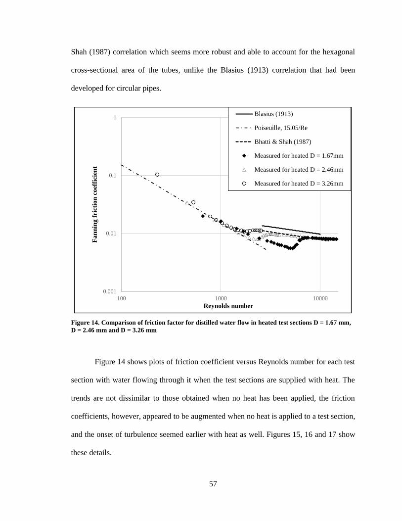
57
Shah (1987) correlation which seems more robust and able to account for the hexagonal
cross-sectional area of the tubes, unlike the Blasius (1913) correlation that had been
developed for circular pipes.
Figure 14. Comparison of friction factor for distilled water flow in heated test sections D = 1.67 mm,
D = 2.46 mm and D = 3.26 mm
Figure 14 shows plots of friction coefficient versus Reynolds number for each test
section with water flowing through it when the test sections are supplied with heat. The
trends are not dissimilar to those obtained when no heat has been applied, the friction
coefficients, however, appeared to be augmented when no heat is applied to a test section,
and the onset of turbulence seemed earlier with heat as well. Figures 15, 16 and 17 show
these details.
0.001
0.01
0.1
1
100 1000 10000
Fa
nn
ing
fri
ctio
n c
oef
fici
ent
Reynolds number
Blasius (1913)
Poiseuille, 15.05/Re
Bhatti & Shah (1987)
Measured for heated D = 1.67mm
Measured for heated D = 2.46mm
Measured for heated D = 3.26mm
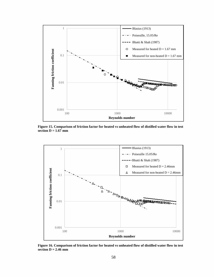
58
Figure 15. Comparison of friction factor for heated vs unheated flow of distilled water flow in test
section D = 1.67 mm
Figure 16. Comparison of friction factor for heated vs unheated flow of distilled water flow in test
section D = 2.46 mm
0.001
0.01
0.1
1
100 1000 10000
Fa
nn
ing
fri
ctio
n c
oef
fici
ent
Reynolds number
Blasius (1913)
Poiseuille, 15.05/Re
Bhatti & Shah (1987)
Measured for heated D = 1.67 mm
Measured for non-heated D = 1.67 mm
0.001
0.01
0.1
1
100 1000 10000
Fa
nn
ing
fri
ctio
n c
oef
fici
ent
Reynolds number
Blasius (1913)
Poiseuille 15.05/Re
Bhatti & Shah (1987)
Measured for heated D = 2.46mm
Measured for non-heated D = 2.46mm
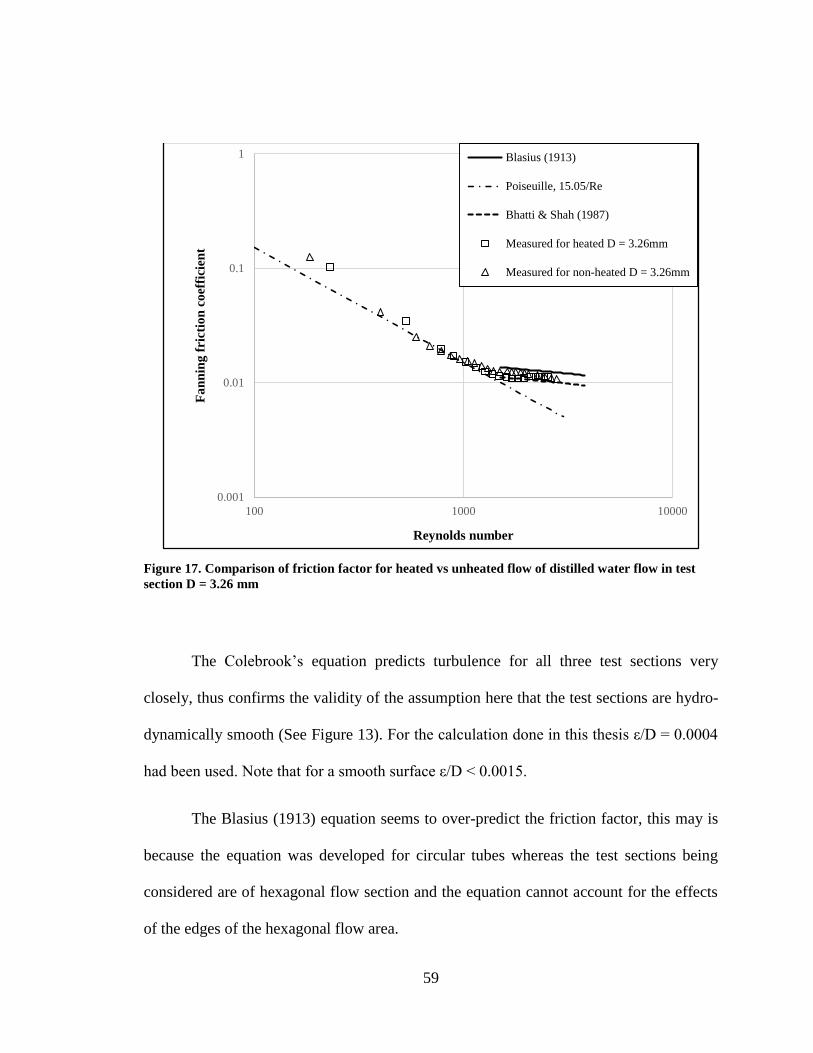
59
Figure 17. Comparison of friction factor for heated vs unheated flow of distilled water flow in test
section D = 3.26 mm
The Colebrook’s equation predicts turbulence for all three test sections very
closely, thus confirms the validity of the assumption here that the test sections are hydro-
dynamically smooth (See Figure 13). For the calculation done in this thesis ε/D = 0.0004
had been used. Note that for a smooth surface ε/D < 0.0015.
The Blasius (1913) equation seems to over-predict the friction factor, this may is
because the equation was developed for circular tubes whereas the test sections being
considered are of hexagonal flow section and the equation cannot account for the effects
of the edges of the hexagonal flow area.
0.001
0.01
0.1
1
100 1000 10000
Fa
nn
ing
fri
ctio
n c
oef
fici
ent
Reynolds number
Blasius (1913)
Poiseuille, 15.05/Re
Bhatti & Shah (1987)
Measured for heated D = 3.26mm
Measured for non-heated D = 3.26mm

60
4.1.2. Heat transfer
The average of the local Nusselt number based on hydraulic diameter against
Reynolds number is shown in Figure 18 for all three test sections as measured water
flowing through each of them. Tests results have been collated for ΔT ≥ 3°C, where ΔT
represents difference between inlet and exit temperature of fluid flowing through a test
section. This is done in order to keep experimental within reasonable limit of error based
on the accuracy of experimental apparatuses.
Figure 18. Comparison of measured Nusselt number vs Reynolds number for distilled water flow
through heated test sections
The measured Nusselt numbers for the laminar and turbulent flow through each test
section is given in the following plots. See Figures 19 and 20, the average Nusselt number
for D = 2.46 mm plotted for specific Reynolds number for the laminar and turbulent flow
5
50
100 1000 10000
Av
erra
ge
Nu
Reynolds number
Measured for D = 1.67mm
Measured for D = 2.46mm
Measured for D = 3.26mm
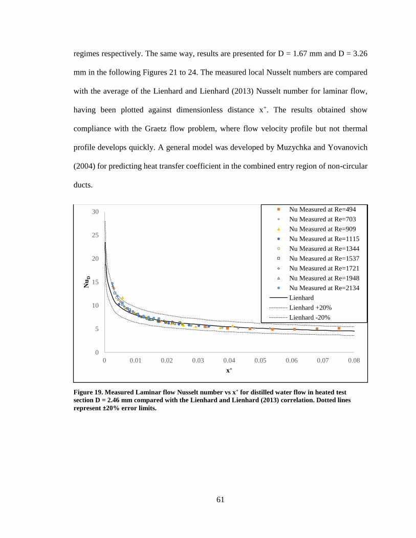
61
regimes respectively. The same way, results are presented for D = 1.67 mm and D = 3.26
mm in the following Figures 21 to 24. The measured local Nusselt numbers are compared
with the average of the Lienhard and Lienhard (2013) Nusselt number for laminar flow,
having been plotted against dimensionless distance x+. The results obtained show
compliance with the Graetz flow problem, where flow velocity profile but not thermal
profile develops quickly. A general model was developed by Muzychka and Yovanovich
(2004) for predicting heat transfer coefficient in the combined entry region of non-circular
ducts.
Figure 19. Measured Laminar flow Nusselt number vs x+ for distilled water flow in heated test
section D = 2.46 mm compared with the Lienhard and Lienhard (2013) correlation. Dotted lines
represent ±20% error limits.
0
5
10
15
20
25
30
0 0.01 0.02 0.03 0.04 0.05 0.06 0.07 0.08
Nu
D
x+
Nu Measured at Re=494
Nu Measured at Re=703
Nu Measured at Re=909
Nu Measured at Re=1115
Nu Measured at Re=1344
Nu Measured at Re=1537
Nu Measured at Re=1721
Nu Measured at Re=1948
Nu Measured at Re=2134
Lienhard
Lienhard +20%
Lienhard -20%
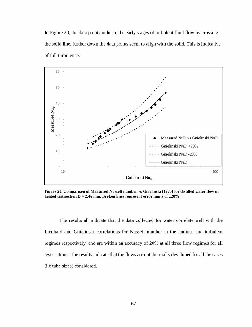
62
In Figure 20, the data points indicate the early stages of turbulent fluid flow by crossing
the solid line, further down the data points seem to align with the solid. This is indicative
of full turbulence.
Figure 20. Comparison of Measured Nusselt number vs Gnielinski (1976) for distilled water flow in
heated test section D = 2.46 mm. Broken lines represent error limits of ±20%
The results all indicate that the data collected for water correlate well with the
Lienhard and Gnielinski correlations for Nusselt number in the laminar and turbulent
regimes respectively, and are within an accuracy of 20% at all three flow regimes for all
test sections. The results indicate that the flows are not thermally developed for all the cases
(i.e tube sizes) considered.
0
10
20
30
40
50
60
10 100
Mea
sure
d N
uD
Gnielinski NuD
Measured NuD vs Gnielinski NuD
Gnielinski NuD +20%
Gnielinski NuD -20%
Gnielinski NuD
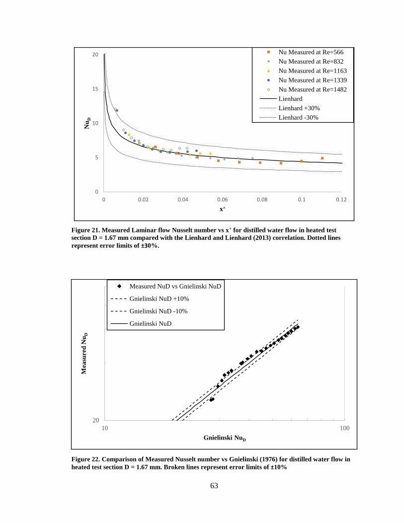
63
Figure 21. Measured Laminar flow Nusselt number vs x+ for distilled water flow in heated test
section D = 1.67 mm compared with the Lienhard and Lienhard (2013) correlation. Dotted lines
represent error limits of ±30%.
Figure 22. Comparison of Measured Nusselt number vs Gnielinski (1976) for distilled water flow in
heated test section D = 1.67 mm. Broken lines represent error limits of ±10%
0
5
10
15
20
0 0.02 0.04 0.06 0.08 0.1 0.12
Nu
D
x+
Nu Measured at Re=566
Nu Measured at Re=832
Nu Measured at Re=1163
Nu Measured at Re=1339
Nu Measured at Re=1482
Lienhard
Lienhard +30%
Lienhard -30%
20
10 100
Mea
sure
d N
uD
Gnielinski NuD
Measured NuD vs Gnielinski NuD
Gnielinski NuD +10%
Gnielinski NuD -10%
Gnielinski NuD
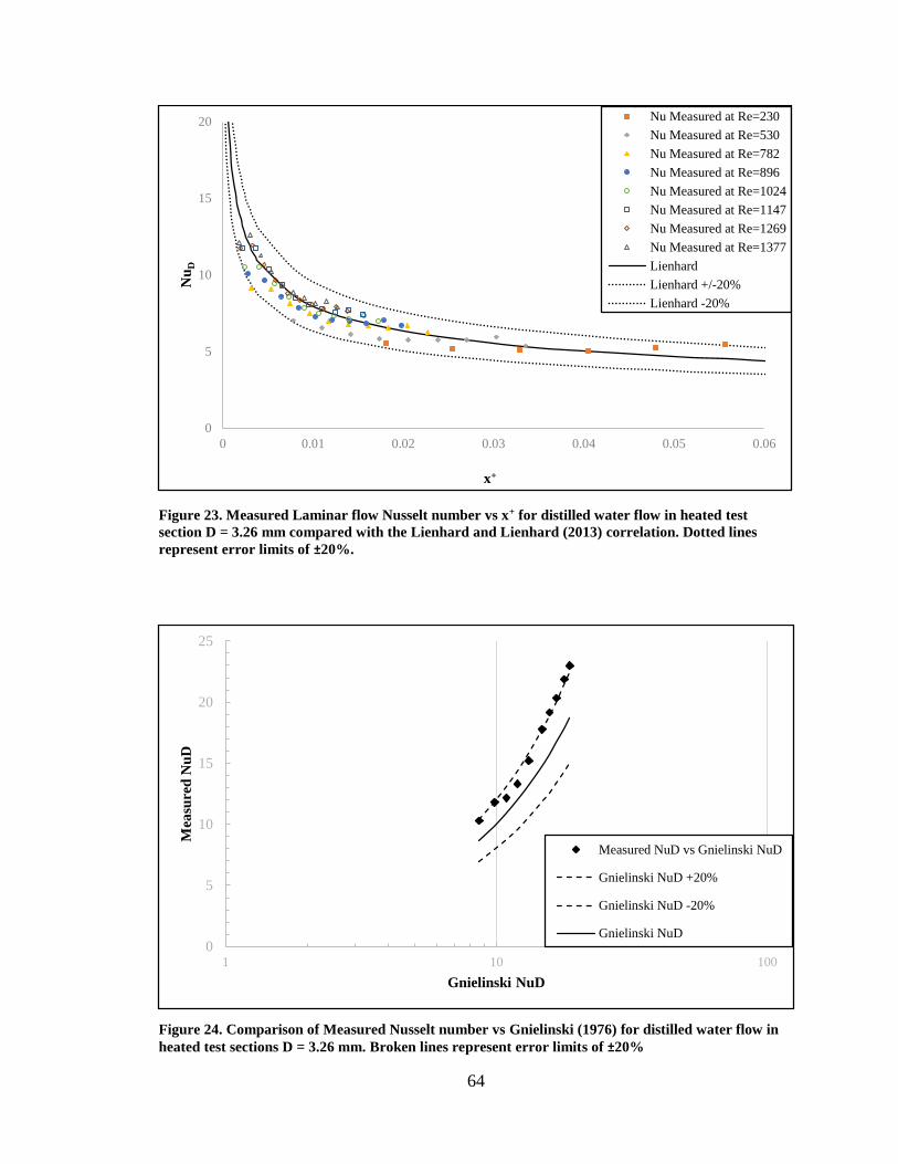
64
Figure 23. Measured Laminar flow Nusselt number vs x+ for distilled water flow in heated test
section D = 3.26 mm compared with the Lienhard and Lienhard (2013) correlation. Dotted lines
represent error limits of ±20%.
Figure 24. Comparison of Measured Nusselt number vs Gnielinski (1976) for distilled water flow in
heated test sections D = 3.26 mm. Broken lines represent error limits of ±20%
0
5
10
15
20
0 0.01 0.02 0.03 0.04 0.05 0.06
Nu
D
x+
Nu Measured at Re=230
Nu Measured at Re=530
Nu Measured at Re=782
Nu Measured at Re=896
Nu Measured at Re=1024
Nu Measured at Re=1147
Nu Measured at Re=1269
Nu Measured at Re=1377
Lienhard
Lienhard +/-20%
Lienhard -20%
0
5
10
15
20
25
1 10 100
Mea
sure
d N
uD
Gnielinski NuD
Measured NuD vs Gnielinski NuD
Gnielinski NuD +20%
Gnielinski NuD -20%
Gnielinski NuD

65
4.2. Nanofluid (9.8% vol. SiO2-water colloid) Results
4.2.1 Friction coefficient
Results obtained for nanofluid show good resemblance to those of water. The trends
are almost identical, although the friction coefficient values for nanofluid appear
augmented compared to distilled water. The inflection points seen on the graphs indicate
the onset of flow regime change.
Figure 25 Comparison of friction factor for nanofluid flow in unheated test sections D = 1.67 mm, D
= 2.46 mm and D = 3.26 mm
As observed for water, the transitioning of nanofluid flow from laminar to
turbulence is more pronounced with decreasing hydraulic diameter, although this happens
0.001
0.01
0.1
1
100 1000 10000
Fa
nn
ing
fri
ctio
n c
oef
fici
ent
Reynolds number
Blasius (1913)
Pouiseuille, 15.05/Re
Bhatti & Shah (1987)
Measured for non-heated D = 1.67 mm
Measured for non-heated D = 2.46 mm
Measured for non-heated D = 3.26 mm
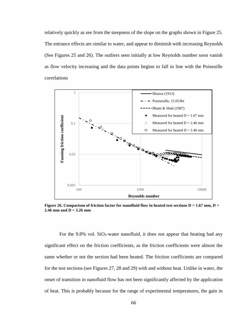
66
relatively quickly as see from the steepness of the slope on the graphs shown in Figure 25.
The entrance effects are similar to water, and appear to diminish with increasing Reynolds
(See Figures 25 and 26). The outliers seen initially at low Reynolds number soon vanish
as flow velocity increasing and the data points beginn to fall in line with the Poiseuille
correlations
Figure 26. Comparison of friction factor for nanofluid flow in heated test sections D = 1.67 mm, D =
2.46 mm and D = 3.26 mm
For the 9.8% vol. SiO2-water nanofluid, it does not appear that heating had any
significant effect on the friction coefficients, as the friction coefficients were almost the
same whether or not the section had been heated. The friction coefficients are compared
for the test sections (see Figures 27, 28 and 29) with and without heat. Unlike in water, the
onset of transition in nanofluid flow has not been significantly affected by the application
of heat. This is probably because for the range of experimental temperatures, the gain in
0.001
0.01
0.1
1
100 1000 10000
Fa
nn
ing
fri
ctio
n c
oef
fici
ent
Reynolds number
Blasius (1913)
Pouiseuille, 15.05/Re
Bhatti & Shah (1987)
Measured for heated D = 1.67 mm
Measured for heated D = 2.46 mm
Measured for heated D = 2.46 mm
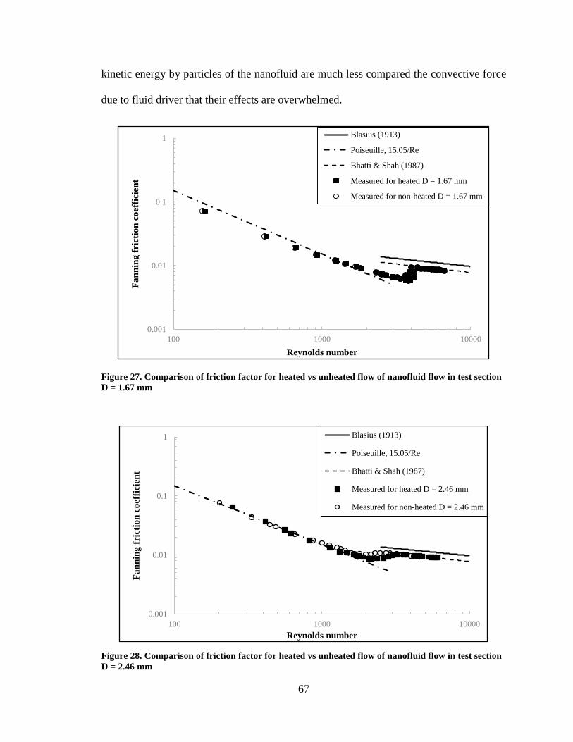
67
kinetic energy by particles of the nanofluid are much less compared the convective force
due to fluid driver that their effects are overwhelmed.
Figure 27. Comparison of friction factor for heated vs unheated flow of nanofluid flow in test section
D = 1.67 mm
Figure 28. Comparison of friction factor for heated vs unheated flow of nanofluid flow in test section
D = 2.46 mm
0.001
0.01
0.1
1
100 1000 10000
Fa
nn
ing
fri
ctio
n c
oef
fici
ent
Reynolds number
Blasius (1913)
Poiseuille, 15.05/Re
Bhatti & Shah (1987)
Measured for heated D = 1.67 mm
Measured for non-heated D = 1.67 mm
0.001
0.01
0.1
1
100 1000 10000
Fa
nn
ing
fri
ctio
n c
oef
fici
ent
Reynolds number
Blasius (1913)
Poiseuille, 15.05/Re
Bhatti & Shah (1987)
Measured for heated D = 2.46 mm
Measured for non-heated D = 2.46 mm
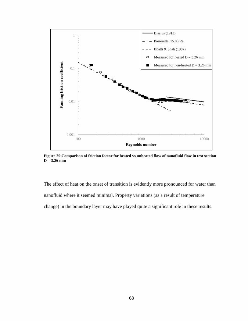
68
Figure 29 Comparison of friction factor for heated vs unheated flow of nanofluid flow in test section
D = 3.26 mm
The effect of heat on the onset of transition is evidently more pronounced for water than
nanofluid where it seemed minimal. Property variations (as a result of temperature
change) in the boundary layer may have played quite a significant role in these results.
0.001
0.01
0.1
1
100 1000 10000
Fa
nn
ing
fri
ctio
n c
oef
fici
ent
Reynolds number
Blasius (1913)
Poiseuille, 15.05/Re
Bhatti & Shah (1987)
Measured for heated D = 3.26 mm
Measured for non-heated D = 3.26 mm

69
4.2.2. Local surface temperature profile for nanofluid flow
The following graphs clearly show the external surface temperature profile of the
nanofluid flow to be consistent with a thermally developing flow. The temperature profile
obviously tends to flatten out at high Reynolds number (or turbulence).
Figure 30. Surface temperature profile for nanofluid flow in test section D = 1.67 mm
The plots of surface temperature profiles for the test sections appear to be consistent with
that of mean fluid temperature for flow through a circular tube in the case of constant
heat flux. This verifies the earlier assumption (see Equation 3.1) that the nanofluid mean
1
10
100
0.1 1T
*=
(Tx/Δ
T)
log(x*)
Re=85
Re=558
Re=1134
Re=2603
Re=4610
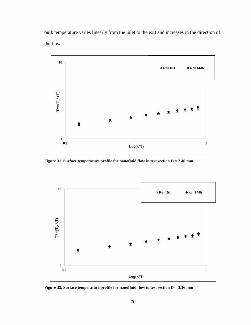
70
bulk temperature varies linearly from the inlet to the exit and increases in the direction of
the flow.
Figure 31. Surface temperature profile for nanofluid flow in test section D = 2.46 mm
Figure 32. Surface temperature profile for nanofluid flow in test section D = 3.26 mm
1
10
0.1 1
T*
=(T
x/Δ
T)
Log(x*))
Re=163 Re=1446
1
10
0.1 1
T*
=(T
x/Δ
T)
Log(x*)
Re=163 Re=1446
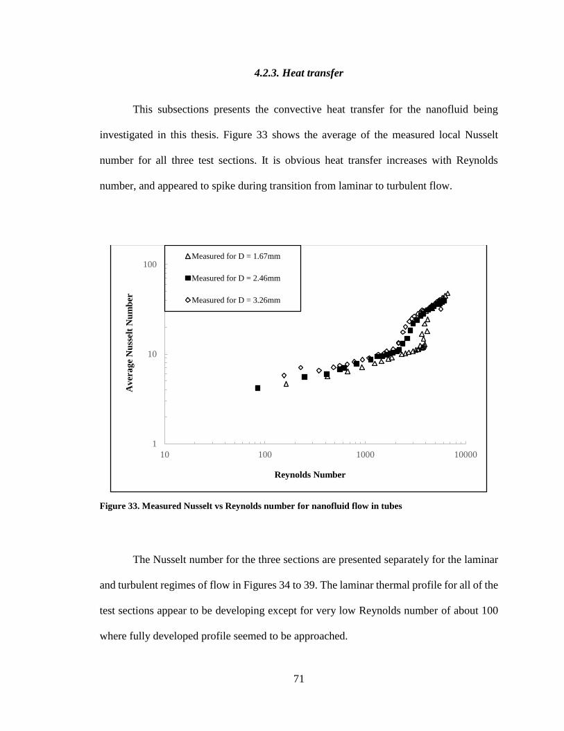
71
4.2.3. Heat transfer
This subsections presents the convective heat transfer for the nanofluid being
investigated in this thesis. Figure 33 shows the average of the measured local Nusselt
number for all three test sections. It is obvious heat transfer increases with Reynolds
number, and appeared to spike during transition from laminar to turbulent flow.
Figure 33. Measured Nusselt vs Reynolds number for nanofluid flow in tubes
The Nusselt number for the three sections are presented separately for the laminar
and turbulent regimes of flow in Figures 34 to 39. The laminar thermal profile for all of the
test sections appear to be developing except for very low Reynolds number of about 100
where fully developed profile seemed to be approached.
1
10
100
10 100 1000 10000
Av
era
ge
Nu
ssel
t N
um
ber
Reynolds Number
Measured for D = 1.67mm
Measured for D = 2.46mm
Measured for D = 3.26mm
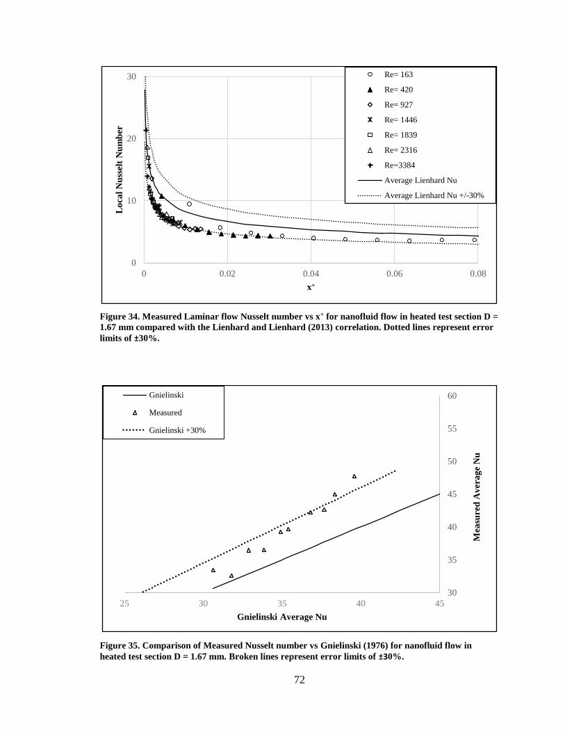
72
Figure 34. Measured Laminar flow Nusselt number vs x+ for nanofluid flow in heated test section D =
1.67 mm compared with the Lienhard and Lienhard (2013) correlation. Dotted lines represent error
limits of ±30%.
Figure 35. Comparison of Measured Nusselt number vs Gnielinski (1976) for nanofluid flow in
heated test section D = 1.67 mm. Broken lines represent error limits of ±30%.
0
10
20
30
0 0.02 0.04 0.06 0.08
Lo
cal
Nu
ssel
t N
um
ber
x+
Re= 163
Re= 420
Re= 927
Re= 1446
Re= 1839
Re= 2316
Re=3384
Average Lienhard Nu
Average Lienhard Nu +/-30%
30
35
40
45
50
55
60
25 30 35 40 45
Mea
sure
d A
ver
ag
e N
u
Gnielinski Average Nu
Gnielinski
Measured
Gnielinski +30%
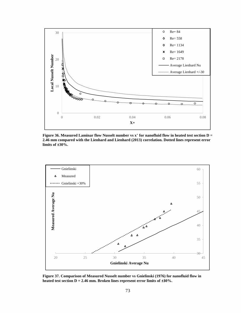
73
Figure 36. Measured Laminar flow Nusselt number vs x+ for nanofluid flow in heated test section D =
2.46 mm compared with the Lienhard and Lienhard (2013) correlation. Dotted lines represent error
limits of ±30%.
Figure 37. Comparison of Measured Nusselt number vs Gnielinski (1976) for nanofluid flow in
heated test section D = 2.46 mm. Broken lines represent error limits of ±30%.
0
10
20
30
0 0.02 0.04 0.06 0.08
Lo
cal
Nu
ssel
t N
um
ber
X+
Re= 84
Re= 558
Re= 1134
Re= 1649
Re= 2178
Average Lienhard Nu
Average Lienhard +/-30
30
35
40
45
50
55
60
20 25 30 35 40 45
Mea
sure
d A
ver
ag
e N
u
Gnielinski Average Nu
Gnielinski
Measured
Gnielinski +30%
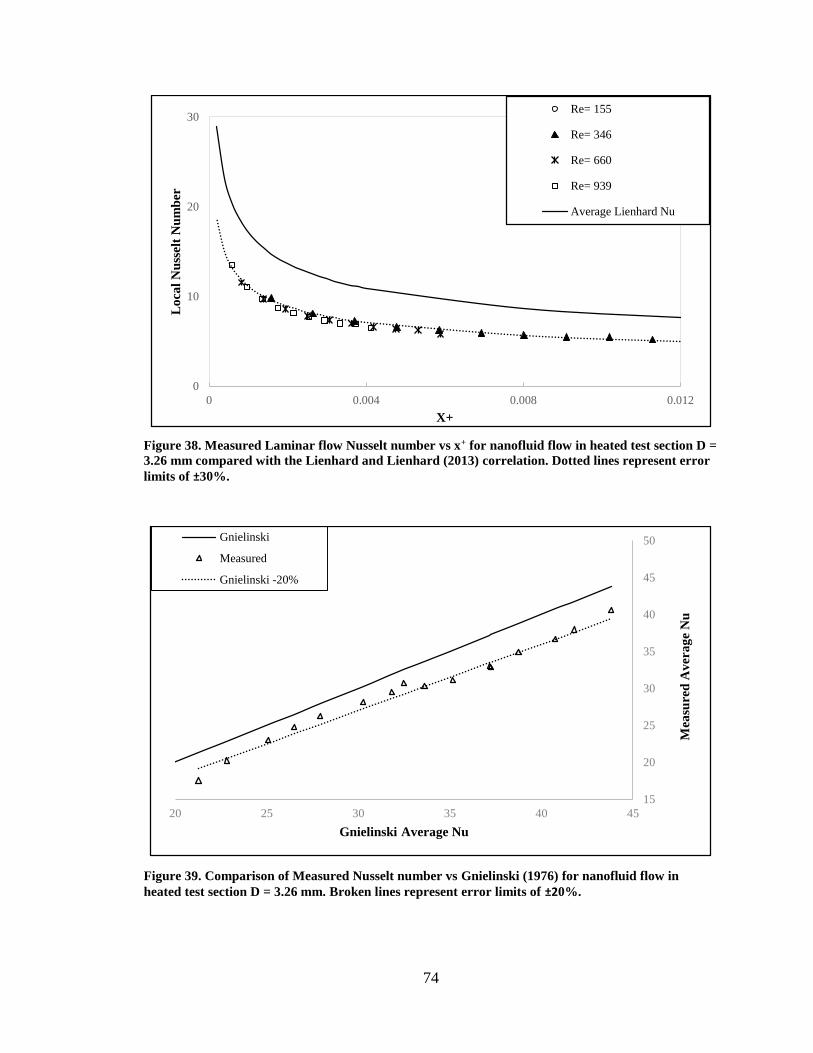
74
Figure 38. Measured Laminar flow Nusselt number vs x+ for nanofluid flow in heated test section D =
3.26 mm compared with the Lienhard and Lienhard (2013) correlation. Dotted lines represent error
limits of ±30%.
Figure 39. Comparison of Measured Nusselt number vs Gnielinski (1976) for nanofluid flow in
heated test section D = 3.26 mm. Broken lines represent error limits of ±20%.
0
10
20
30
0 0.004 0.008 0.012
Lo
cal
Nu
ssel
t N
um
ber
X+
Re= 155
Re= 346
Re= 660
Re= 939
Average Lienhard Nu
15
20
25
30
35
40
45
50
20 25 30 35 40 45
Mea
sure
d A
ver
ag
e N
u
Gnielinski Average Nu
Gnielinski
Measured
Gnielinski -20%
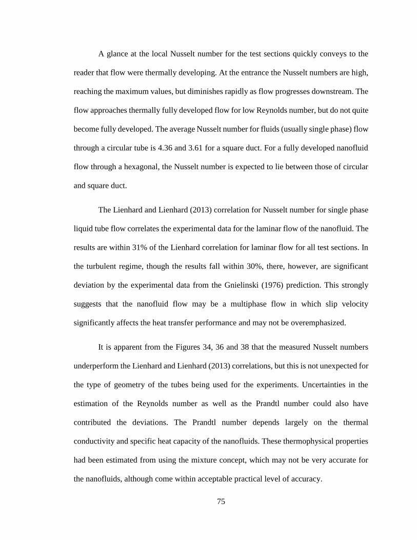
75
A glance at the local Nusselt number for the test sections quickly conveys to the
reader that flow were thermally developing. At the entrance the Nusselt numbers are high,
reaching the maximum values, but diminishes rapidly as flow progresses downstream. The
flow approaches thermally fully developed flow for low Reynolds number, but do not quite
become fully developed. The average Nusselt number for fluids (usually single phase) flow
through a circular tube is 4.36 and 3.61 for a square duct. For a fully developed nanofluid
flow through a hexagonal, the Nusselt number is expected to lie between those of circular
and square duct.
The Lienhard and Lienhard (2013) correlation for Nusselt number for single phase
liquid tube flow correlates the experimental data for the laminar flow of the nanofluid. The
results are within 31% of the Lienhard correlation for laminar flow for all test sections. In
the turbulent regime, though the results fall within 30%, there, however, are significant
deviation by the experimental data from the Gnielinski (1976) prediction. This strongly
suggests that the nanofluid flow may be a multiphase flow in which slip velocity
significantly affects the heat transfer performance and may not be overemphasized.
It is apparent from the Figures 34, 36 and 38 that the measured Nusselt numbers
underperform the Lienhard and Lienhard (2013) correlations, but this is not unexpected for
the type of geometry of the tubes being used for the experiments. Uncertainties in the
estimation of the Reynolds number as well as the Prandtl number could also have
contributed the deviations. The Prandtl number depends largely on the thermal
conductivity and specific heat capacity of the nanofluids. These thermophysical properties
had been estimated from using the mixture concept, which may not be very accurate for
the nanofluids, although come within acceptable practical level of accuracy.
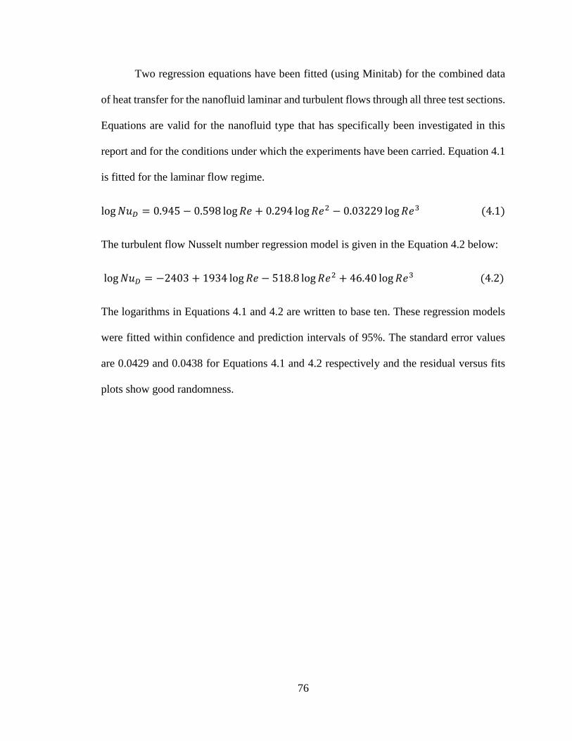
76
Two regression equations have been fitted (using Minitab) for the combined data
of heat transfer for the nanofluid laminar and turbulent flows through all three test sections.
Equations are valid for the nanofluid type that has specifically been investigated in this
report and for the conditions under which the experiments have been carried. Equation 4.1
is fitted for the laminar flow regime.
log 𝑁𝑢𝐷 = 0.945 − 0.598 log 𝑅𝑒 + 0.294 log 𝑅𝑒2 − 0.03229 log 𝑅𝑒3 (4.1)
The turbulent flow Nusselt number regression model is given in the Equation 4.2 below:
log 𝑁𝑢𝐷 = −2403 + 1934 log 𝑅𝑒 − 518.8 log 𝑅𝑒2 + 46.40 log 𝑅𝑒3 (4.2)
The logarithms in Equations 4.1 and 4.2 are written to base ten. These regression models
were fitted within confidence and prediction intervals of 95%. The standard error values
are 0.0429 and 0.0438 for Equations 4.1 and 4.2 respectively and the residual versus fits
plots show good randomness.
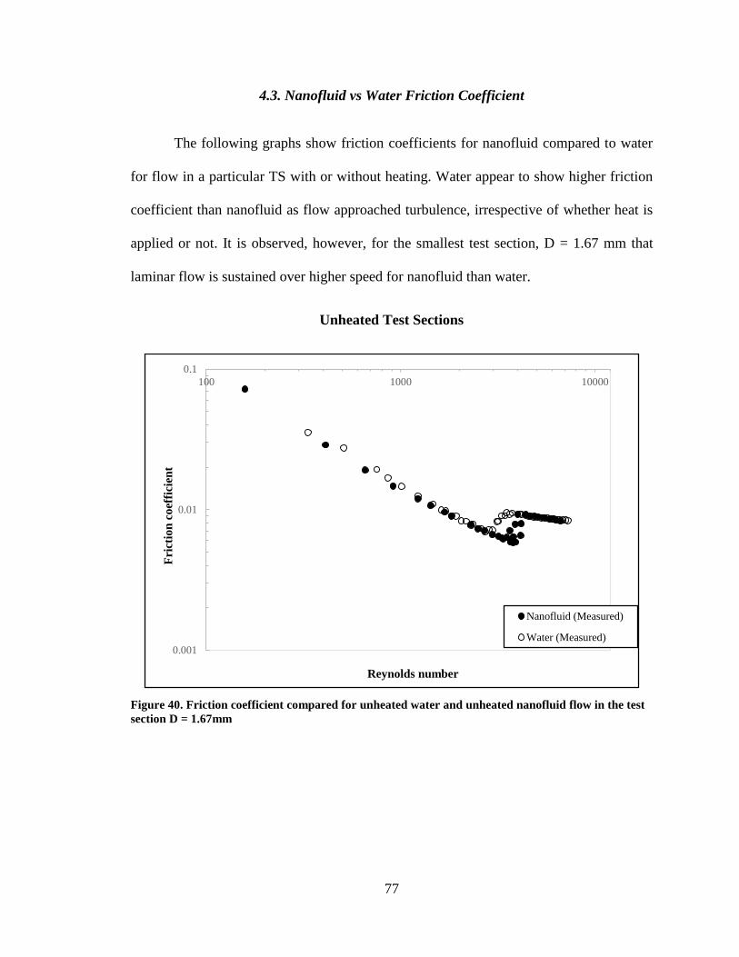
77
4.3. Nanofluid vs Water Friction Coefficient
The following graphs show friction coefficients for nanofluid compared to water
for flow in a particular TS with or without heating. Water appear to show higher friction
coefficient than nanofluid as flow approached turbulence, irrespective of whether heat is
applied or not. It is observed, however, for the smallest test section, D = 1.67 mm that
laminar flow is sustained over higher speed for nanofluid than water.
Unheated Test Sections
Figure 40. Friction coefficient compared for unheated water and unheated nanofluid flow in the test
section D = 1.67mm
0.001
0.01
0.1
100 1000 10000
Fri
ctio
n c
oef
fici
ent
Reynolds number
Nanofluid (Measured)
Water (Measured)
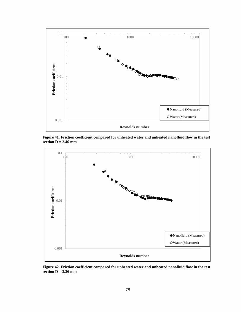
78
Figure 41. Friction coefficient compared for unheated water and unheated nanofluid flow in the test
section D = 2.46 mm
Figure 42. Friction coefficient compared for unheated water and unheated nanofluid flow in the test
section D = 3.26 mm
0.001
0.01
0.1
100 1000 10000
Fri
ctio
n c
oef
fici
ent
Reynolds number
Nanofluid (Measured)
Water (Measured)
0.001
0.01
0.1
100 1000 10000
Fri
ctio
n c
oef
fici
ent
Reynolds number
Nanofluid (Measured)
Water (Measured)
79
Nanofluid transitions later than water when test section is not heated, this
phenomenon appears to be more pronounced with smaller tube hydraulic diameter (see
Figure 40). But, it is the exact opposite when heat is applied, as the results show that water
sustains laminar flow longer than nanofluid for smaller hydraulic diameter. These
observations raise concerns about the effect of nanoparticle movements on the
characteristics of the flow.
Heated Test Sections
Figure 43. Friction coefficient compared for heated water and heated nanofluid flow in test section D
= 1.67 mm
0.001
0.01
0.1
100 1000 10000
Fri
ctio
n c
oef
fici
ent
Reynolds number
Nanofluid (Measured)
Water (Measured)
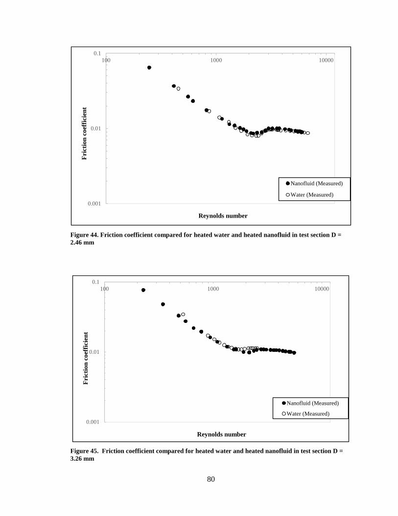
80
Figure 44. Friction coefficient compared for heated water and heated nanofluid in test section D =
2.46 mm
Figure 45. Friction coefficient compared for heated water and heated nanofluid in test section D =
3.26 mm
0.001
0.01
0.1
100 1000 10000
Fri
ctio
n c
oef
fici
ent
Reynolds number
Nanofluid (Measured)
Water (Measured)
0.001
0.01
0.1
100 1000 10000
Fri
ctio
n c
oef
fici
ent
Reynolds number
Nanofluid (Measured)
Water (Measured)
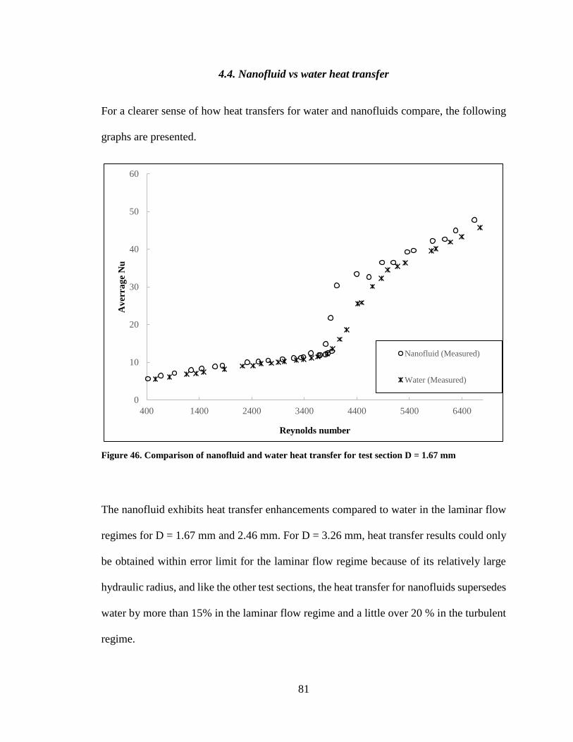
81
4.4. Nanofluid vs water heat transfer
For a clearer sense of how heat transfers for water and nanofluids compare, the following
graphs are presented.
Figure 46. Comparison of nanofluid and water heat transfer for test section D = 1.67 mm
The nanofluid exhibits heat transfer enhancements compared to water in the laminar flow
regimes for D = 1.67 mm and 2.46 mm. For D = 3.26 mm, heat transfer results could only
be obtained within error limit for the laminar flow regime because of its relatively large
hydraulic radius, and like the other test sections, the heat transfer for nanofluids supersedes
water by more than 15% in the laminar flow regime and a little over 20 % in the turbulent
regime.
0
10
20
30
40
50
60
400 1400 2400 3400 4400 5400 6400
Av
erra
ge
Nu
Reynolds number
Nanofluid (Measured)
Water (Measured)
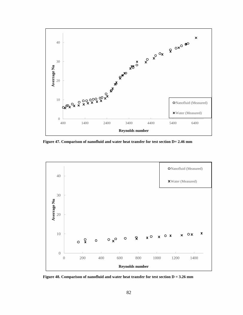
82
Figure 47. Comparison of nanofluid and water heat transfer for test section D= 2.46 mm
Figure 48. Comparison of nanofluid and water heat transfer for test section D = 3.26 mm
0
10
20
30
40
400 1400 2400 3400 4400 5400 6400
Av
erra
ge
Nu
Reynolds number
Nanofluid (Measured)
Water (Measured)
0
10
20
30
40
0 200 400 600 800 1000 1200 1400
Av
erra
ge
Nu
Reynolds number
Nanofluid (Measured)
Water (Measured)
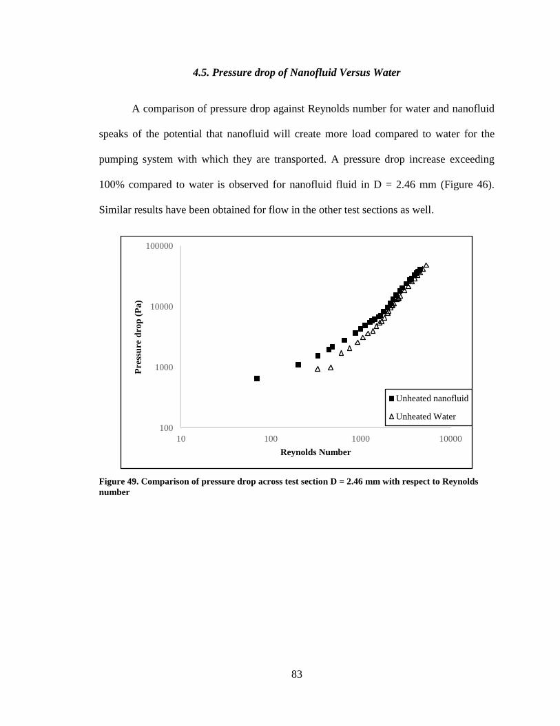
83
4.5. Pressure drop of Nanofluid Versus Water
A comparison of pressure drop against Reynolds number for water and nanofluid
speaks of the potential that nanofluid will create more load compared to water for the
pumping system with which they are transported. A pressure drop increase exceeding
100% compared to water is observed for nanofluid fluid in D = 2.46 mm (Figure 46).
Similar results have been obtained for flow in the other test sections as well.
Figure 49. Comparison of pressure drop across test section D = 2.46 mm with respect to Reynolds
number
100
1000
10000
100000
10 100 1000 10000
Pre
ssu
re d
rop
(P
a)
Reynolds Number
Unheated nanofluid
Unheated Water

84
Figure 50 Comparison of pressure drop across test section D = 1.67 mm with respect to Reynolds
number
Figure 51. Comparison of pressure drop across test section D = 3.26 mm with respect to Reynolds
number
100
10000
1000000
100 1000 10000
Pre
ssu
re d
rop
(P
a)
Reynolds number
Unheated nanofluid
Unheated water
100
1000
10000
100000
100 1000 10000
Unheated nanofluid
Unheated water
85
CHAPTER V
CONCLUSIONS AND RECOMMENDATIONS
5.1. Conclusions
The flow and heat transfer characteristics of silicon-dioxide water-based nanofluid
in three different sized brass hexagonal tubes have been closely monitored during the
experimentations carried out in this thesis. Flows were operated for the range of Reynolds
number 400-8000, encompassing the laminar, transitional and turbulent flow regimes.
Primarily, pressure drops and tube surface temperatures are the focal parameters through
which the fluid characterizations have essentially been drawn or estimated. Reynolds
number were controlled by adjusting the rotor speed of the variable speed feed
water/nanofluid gear pump.
The Metzner and Reed (1955) correlation proved good for estimating Reynolds
number in the laminar flow regime, with a reasonable degree of accuracy in the transition
and turbulent flow regimes for water. These experimentations with water are a rigorous
method by which the procedures and methods of experiments have been validated in this
thesis. It predicts Reynolds number with an accuracy of 90-95% in the laminar regime and
between 80 and 85% for the turbulent and the transition regimes.
86
The pressure drop and heat transfer characteristics of SiO2-water-based nanofluid
flow inside horizontal hexagonal duct brass tubes are investigated for the entrance region.
The nanofluid friction coefficients are well correlated by classical single phase fluid
correlations suggesting that the nanofluid can very well be treated as single phase fluid
rather a mixture.
The nanofluid appears to longer sustain laminar flow (with transition occurring at
higher speed or Reynolds number) when fluid is not being heated, while offering superior
heat transfer than water. This is a pointer to more prominent shear stress on the wall of
smaller test section than the larger ones. On the other hand, upon applying heat to the flow
system, water transitioned much later than nanofluid in the smallest tube flow and does
exhibit more drag on the wall as indicated by the higher friction coefficient in the laminar
flow regime. This is suggestive of a possible net migration of nanoparticles from the wall
toward the axis of the flow, it makes one to wonder whether the time of travel of particle
from the flow axis to the core might be a contributing factor as well.
The measured results showed high convective heat transfer at high Reynolds
numbers, having been compared with the classical correlations, the turbulent heat transfer
results were not closely correlated by the classical equations. The observed heat transfer
enhancements for high Reynolds number could be due to persistent thermal dispersion
which may have been induced by intensified micro-convection and diffusion of
nanoparticles at high flow velocities as a result of the effect of temperature gradient on the
properties of the nanofluid. As expected, the heat transfers were higher for increasing
hydraulic diameters of flow tubes.
87
Migration of nanofluid particles may be responsible for wearing the viscous
boundary layer much faster than for water for which molecules have a higher degree of
freedom and much more elastic. The high momentum of nanoparticles at high flow rate
may allow them to easily penetrate the laminar boundary layer, and upon heating the
particles the gain kinetic energy as well. These inferences are, however, inconclusive
without more evidence.
The diminishment in the friction coefficient (probably as a result of depletion of
boundary layer as a consequence of particle migration could have led to the fluid losing
contact with the flow surface or introducing slip flow resulting in cavitation effect on the
surface) can cause localized overheating and cavitation effects on the heat transfer surface.
The large pressure drops for nanofluid flow may be attributed to reversal of flow and
collision drag. But it is just not the separation of the flow at the wall that should be
considered in the study of nanofluid, the interaction of the solid-fluid surface is likely very
significant to the heat transfer mechanisms.
Whereas, heat transfer enhancements have been recorded for nanofluid, such
enhancements may not be worth the troubles for the corresponding pressure drops
(reaching over 60% compared with water) associated with the fluid flows. These high
pressure drops leave a dilemma for design of nanofluid heat transfer systems with respect
to energy requirements. It is obvious, nanofluid heat exchange systems would require more
pumping power to transport the fluid.

88
5.2. Recommendations and Future Work
More studies need to be conducted to determine what mechanisms are responsible
for the flow transitions associated with nanofluids or the heat transfer enhancements for
that matter. In the future, more effective method like use of particles size analyzer, electron
microscopy (SEM-scanning electron microscope, TEM- transmission electron microscopy
will be utilized in the determination of the distribution of nanofluid particle size and
aggregates to increase the odds of correctly characterizing the fluid (especially for high
concentration of particles). A dispersion model may also be applied in the investigation of
the heat transfer mechanisms of nanofluids.
Future work will also include the measurement of pressure drop at multiple
locations along the length of the tube. This will be done by fabricating specially shaped
pressure tap holes that will enable pressure measurements to be taken without distorting
the flow. The use of infrared to measured heat distribution throughout flow domain will
also be considered.
The use of peristaltic pump for future work is recommended for more smooth flow.
Also, the use of transparent test section and high speed and thermal imaging could prove
pivotal in the study of flow and heat transfer mechanisms of the nanofluid.
The approximation of nanofluid as a single phase fluid does have many setbacks
especially for high speed flow where compression wave phenomenon for instance would
have to be accounted for. Stabilizers or surfactants can effectively change the phase
distribution of the nanofluid systems and should be investigated for contribution to the
surface tension behavior of the fluid. The overall effect of surfactant concentration on the

89
thermophysical properties of the nanofluid especially where there may be boiling heat
transfer or two phase heat transfer should be investigated as well.
Multiple run of experiments will be done for future experiments to allow for more
encompassing and comprehensive investigation of uncertainty to be carried out. Also, there
is need to investigate a wider concentrations of the nanofluid to obtain more information
on the nanofluid properties and allow for an extended range over which these properties
and the dependencies may be more accurately predicted. Working with different
concentrations may also help to determine the effect of particle concentration on the length
of the region. Carrying experiments for multiple nanoparticle concentrations can be of
much help to validating such claims as the effect of particle concentration and mobility on
the onset and intensity of turbulence.
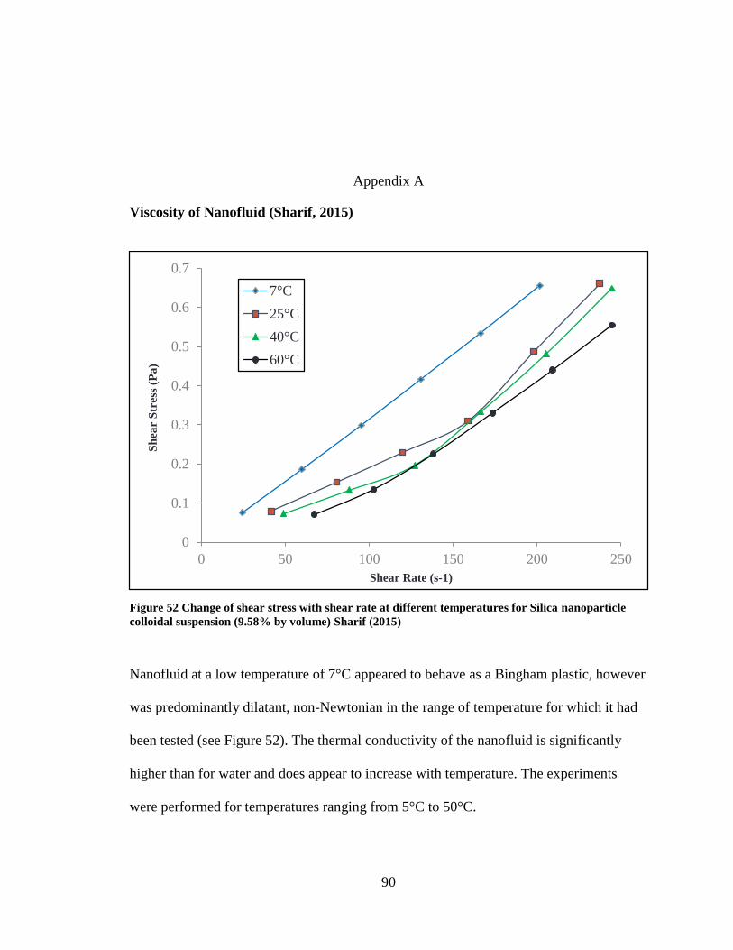
90
Appendix A
Viscosity of Nanofluid (Sharif, 2015)
Figure 52 Change of shear stress with shear rate at different temperatures for Silica nanoparticle
colloidal suspension (9.58% by volume) Sharif (2015)
Nanofluid at a low temperature of 7°C appeared to behave as a Bingham plastic, however
was predominantly dilatant, non-Newtonian in the range of temperature for which it had
been tested (see Figure 52). The thermal conductivity of the nanofluid is significantly
higher than for water and does appear to increase with temperature. The experiments
were performed for temperatures ranging from 5°C to 50°C.
0
0.1
0.2
0.3
0.4
0.5
0.6
0.7
0 50 100 150 200 250
Sh
ear
Str
ess
(Pa
)
Shear Rate (s-1)
7°C
25°C
40°C
60°C
91
Appendix B
Error Analysis
While the experiments conducted here have be performed with great care, the
possibility of errors within the results cannot be overlooked. Errors could be due to
inefficiencies in data acquisition procedure, fabrication of system components or human
errors. (Note that instrument precision or error of measurement are given in Table 1).
Consequently, steps have been taken to minimize these errors. Multiple data points were
collected and averaged to minimize bias errors in measurements thus it has been assumed
for the directly measured data that fixed errors or biases are negligible and only random
(or precision) errors significant in the analysis. Though the root sum square (RSS) method
by Moffat (1982) and Moffat (1988) could not be employed to perform further analysis of
uncertainty since there were no multiple runs or replicates for the experiment, the analysis
however, follows their prescribed method for reporting uncertainty.
Apparent Viscosity, Reynolds Number and Friction Factors Uncertainty
The uncertainty in the Reynolds number comes from the assumption of constant
apparent viscosity and density over a wide range of shear stress (see Equations 3.4 and
3.5), however, is a reasonable one from the practical point of view, having been validated
by comparing results with data from well-established literature for water. The uncertainty
of the density of the nanofluid is estimated at 1.69% by Sharif (2015).
92
The friction factor uncertainty obviously depends on the accuracy of measuring
pressure drop, the hydraulic diameter and length of the test section and the fluid’s density
as well as the mass flow rate. The uncertainty of the pressure drop measurements are given
by Tiwari (2012) as ±40.43Pa. The width tolerance for the test sections are specified at
±0.002 inches and that of the thickness at ±0.001 inches by the manufacturer.
Experiments reveal, however, a vast spectrum of non-Newtonian fluids may be
represented over wide ranges of shear rate by a two-constant power law. While a fluid may
fall into a category of classification, rheological properties or even assigned values
resulting from such classifications appear to be very sensitive to the conditions of
experiment under which they are developed; without care, such classifications could result
in the oversimplification Metzner and Reed (1955). The nanofluids presented have been
found to be time-independent in nature from the experiments conducted by Sharif (2015).
93
REFERENCES
Aladag, B., Halelfadl, S., Doner, N., Maré, T., Duret, S., & Estellé, P. (2012). Experimental
investigations of the viscosity of nanofluids at low temperatures. Applied Energy, 97,
876-880.
Assael, M., Metaxa, I., Kakosimos, K., & Constantinou, D. (2006). Thermal conductivity
of nanofluids–experimental and theoretical. International Journal of Thermophysics,
27(4), 999-1017.
Azizian, R., Doroodchi, E., McKrell, T., Buongiorno, J., Hu, L., & Moghtaderi, B. (2014).
Effect of magnetic field on laminar convective heat transfer of magnetite nanofluids.
International Journal of Heat and Mass Transfer, 68, 94-109.
Baby, T. T., & Ramaprabhu, S. (2011). Synthesis and nanofluid application of silver
nanoparticles decorated graphene. Journal of Materials Chemistry, 21(26), 9702-
9709.
Beck, M. P., Yuan, Y., Warrier, P., & Teja, A. S. (2009). The effect of particle size on the
thermal conductivity of alumina nanofluids. Journal of Nanoparticle Research, 11(5),
1129-1136.
Bhatti, M., & Shah, R. (1987). Turbulent and transition flow convective heat transfer in
ducts. Handbook of Single-Phase Convective Heat Transfer, , 4.1-4.166.
Blasius, H. (1913). Das ähnlichkeitsgesetz bei reibungsvorgängen in flüssigkeiten
Springer.
Brintlinger, T., Qi, Y., Baloch, K. H., Goldhaber-Gordon, D., & Cumings, J. (2008).
Electron thermal microscopy. Nano Letters, 8(2), 582-585.
Brkić, D. (2011). Review of explicit approximations to the colebrook relation for flow
friction. Journal of Petroleum Science and Engineering, 77(1), 34-48.
Buongiorno, J. (2006). Convective transport in nanofluids. Journal of Heat Transfer,
128(3), 240-250.
Çengel, Y. A., & Ghajar, A. J. (2011). Heat and mass transfer: Fundamentals &
applications McGraw-Hill.
94
Choi, S. U. S., & Eastman, J. A. (1995). Enhancing thermal conductivity of fluids with
nanoparticles. Paper presented at the 1995 International Mechanical Engineering
Congress and Exhibition, San Francisco, CA (United States), 12-17 Nov 1995, pp. 99-
106.
Colebrook, C., & White, C. (1937). Experiments with fluid friction in roughened pipes.
Proceedings of the Royal Society of London.Series a, Mathematical and Physical
Sciences, , 367-381.
Das, S. K., Putra, N., & Roetzel, W. (2003). Pool boiling characteristics of nano-fluids.
International Journal of Heat and Mass Transfer, 46(5), 851-862.
Das, S. K., Putra, N., Thiesen, P., & Roetzel, W. (2003). Temperature dependence of
thermal conductivity enhancement for nanofluids. Journal of Heat Transfer, 125(4),
567-574.
Dodge, D., & Metzner, A. (1959). Turbulent flow of non‐Newtonian systems. AIChE
Journal, 5(2), 189-204.
Duangthongsuk, W., & Wongwises, S. (2010). An experimental study on the heat transfer
performance and pressure drop of TiO 2-water nanofluids flowing under a turbulent
flow regime. International Journal of Heat and Mass Transfer, 53(1), 334-344.
Einstein, A. (1906). A new determination of molecular dimensions. Ann.Phys, 19(2), 289-
306.
Fakoor-Pakdaman, M., Akhavan-Behabadi, M., & Razi, P. (2013). An empirical study on
the pressure drop characteristics of nanofluid flow inside helically coiled tubes.
International Journal of Thermal Sciences, 65, 206-213.
Fedele, L., Colla, L., Bobbo, S., Barison, S., & Agresti, F. (2011). Experimental stability
analysis of different water-based nanofluids. Nanoscale Research Letters, 6(1), 1-8.
Fotukian, S., & Esfahany, M. N. (2010). Experimental study of turbulent convective heat
transfer and pressure drop of dilute CuO/water nanofluid inside a circular tube.
International Communications in Heat and Mass Transfer, 37(2), 214-219.
Fotukian, S., & Esfahany, M. N. (2010). Experimental study of turbulent convective heat
transfer and pressure drop of dilute CuO/water nanofluid inside a circular tube.
International Communications in Heat and Mass Transfer, 37(2), 214-219.
Ghadimi, A., Saidur, R., & Metselaar, H. (2011). A review of nanofluid stability properties
and characterization in stationary conditions. International Journal of Heat and Mass
Transfer, 54(17), 4051-4068.
95
Gnielinski, V. (1976). New equations for heat and mass-transfer in turbulent pipe and
channel flow. International Chemical Engineering, 16(2), 359-368.
Haynes, W. M. (2013). CRC handbook of chemistry and physics CRC press.
Heris, S. Z., Etemad, S. G., & Esfahany, M. N. (2006). Experimental investigation of oxide
nanofluids laminar flow convective heat transfer. International Communications in
Heat and Mass Transfer, 33(4), 529-535.
Howe, K. J., Hand, D. W., Crittenden, J. C., Trussell, R. R., & Tchobanoglous, G. (2012).
Principles of water treatment John Wiley & Sons.
Hussein, A. M., Sharma, K., Bakar, R., & Kadirgama, K. (2014). A review of forced
convection heat transfer enhancement and hydrodynamic characteristics of a
nanofluid. Renewable and Sustainable Energy Reviews, 29, 734-743.
Jiang, L., Gao, L., & Sun, J. (2003). Production of aqueous colloidal dispersions of carbon
nanotubes. Journal of Colloid and Interface Science, 260(1), 89-94.
Joshi, M., Bhattacharyya, A., & Ali, S. W. (2008). Characterization techniques for
nanotechnology applications in textiles. Indian Journal of Fibre and Textile Research,
33(3), 304-317.
Kabelac, S., & Kuhnke, J. (2006). Heat transfer mechanisms in nanofluids--experiments
and theory--. Paper presented at the International Heat Transfer Conference 13,
Kakaç, S., & Pramuanjaroenkij, A. (2009). Review of convective heat transfer
enhancement with nanofluids. International Journal of Heat and Mass Transfer,
52(13), 3187-3196.
Kays, W. M., Crawford, M. E., & Weigand, B. (2012). Convective heat and mass transfer
Tata McGraw-Hill Education.
Keblinski, P., Eastman, J. A., & Cahill, D. G. (2005). Nanofluids for thermal transport.
Materials Today, 8(6), 36-44.
Kestin, J., Mordechai, S., & William A, W. (1978). Viscosity of liquid water in the range−
8 C to 150 C. Journal of Physical and Chemical Reference Data, 7(3), 941-948.
Kole, M., & Dey, T. (2010). Viscosity of alumina nanoparticles dispersed in car engine
coolant. Experimental Thermal and Fluid Science, 34(6), 677-683.
Kothandaraman, C. (2004). Heat and mass transfer data book New Age International.
Krishnamurthy, S., Bhattacharya, P., Phelan, P., & Prasher, R. (2006). Enhanced mass
transport in nanofluids. Nano Letters, 6(3), 419-423.

96
Lee, S., Choi, S., Li, S., and, & Eastman, J. (1999). Measuring thermal conductivity of
fluids containing oxide nanoparticles. Journal of Heat Transfer, 121(2), 280-289.
Lee, S. W., Park, S. D., Kang, S., Bang, I. C., & Kim, J. H. (2011). Investigation of
viscosity and thermal conductivity of SiC nanofluids for heat transfer applications.
International Journal of Heat and Mass Transfer, 54(1), 433-438.
Li, W., & Wu, Z. (2010). A general criterion for evaporative heat transfer in micro/mini-
channels. International Journal of Heat and Mass Transfer, 53(9), 1967-1976.
Lienhard, J., & Lienhard, J. (2013). A heat transfer textbook Courier Corporation.
Maiga, S. E. B., Palm, S. J., Nguyen, C. T., Roy, G., & Galanis, N. (2005). Heat transfer
enhancement by using nanofluids in forced convection flows. International Journal
of Heat and Fluid Flow, 26(4), 530-546.
Maxwell, J. C., & Thompson, J. J. (1892). A treatise on electricity and magnetism
Clarendon.
McNab, G., & Meisen, A. (1973). Thermophoresis in liquids. Journal of Colloid and
Interface Science, 44(2), 339-346.
Metzner, A., & Reed, J. (1955). Flow of non‐newtonian fluids—correlation of the laminar,
transition, and turbulent‐flow regions. AIChE Journal, 1(4), 434-440.
Moffat, R. (1982). Contributions to the theory of single-sample uncertainty analysis.
ASME, Transactions, Journal of Fluids Engineering, 104(2), 250-258.
Moffat, R. J. (1988). Describing the uncertainties in experimental results. Experimental
Thermal and Fluid Science, 1(1), 3-17.
Muzychka, Y., & Yovanovich, M. (2004). Laminar forced convection heat transfer in the
combined entry region of non-circular ducts. Journal of Heat Transfer, 126(1), 54-61.
Namburu, P. K., Kulkarni, D. P., Misra, D., & Das, D. K. (2007). Viscosity of copper oxide
nanoparticles dispersed in ethylene glycol and water mixture. Experimental Thermal
and Fluid Science, 32(2), 397-402.
Pak, B. C., & Cho, Y. I. (1998). Hydrodynamic and heat transfer study of dispersed fluids
with submicron metallic oxide particles. Experimental Heat Transfer an International
Journal, 11(2), 151-170.
Phuoc, T. X., & Massoudi, M. (2009). Experimental observations of the effects of shear
rates and particle concentration on the viscosity of fe 2 O 3–deionized water
nanofluids. International Journal of Thermal Sciences, 48(7), 1294-1301.
97
Sahooli, M., Sabbaghi, S., & Shariaty Niassar, M. (2012). Preparation of CuO/Water
nanofluids using polyvinylpyrolidone and a survey on its stability and thermal
conductivity. International Journal of Nanoscience and Nanotechnology, 8(1), 27-34.
Schwartz, L. M., Garboczi, E. J., & Bentz, D. P. (1995). Interfacial transport in porous
media: Application to dc electrical conductivity of mortars. Journal of Applied
Physics, 78(10), 5898-5908.
Sharrif, T. (2015). Experimental investigation of thermophysical poperties, pressure drop
and heat transfer of non-newtonian silica colloid flow in tubes. (Masters, University
of North Dakota).
Shaver, R. G., & Merrill, E. W. (1959). Turbulent flow of pseudoplastic polymer solutions
in straight cylindrical tubes. AIChE Journal, 5(2), 181-188.
Sundar, L. S., & Singh, M. K. (2013). Convective heat transfer and friction factor
correlations of nanofluid in a tube and with inserts: A review. Renewable and
Sustainable Energy Reviews, 20, 23-35.
Timofeeva, E. V., Smith, D. S., Yu, W., France, D. M., Singh, D., & Routbort, J. L. (2010).
Particle size and interfacial effects on thermo-physical and heat transfer characteristics
of water-based α-SiC nanofluids. Nanotechnology, 21(21), 215703.
Tiwari, S. (2012). Evaluation of thermophysical properties, friction factor, and heat transfer
of alumina nanofluid flow in tubes. (Masters, University of North Dakota, Grand
Forks).
Vajjha, R. S., & Das, D. K. (2009). Specific heat measurement of three nanofluids and
development of new correlations. Journal of Heat Transfer, 131(7), 071601.
Wang, B., Zhou, L., & Peng, X. (2003). A fractal model for predicting the effective thermal
conductivity of liquid with suspension of nanoparticles. International Journal of Heat
and Mass Transfer, 46(14), 2665-2672.
Wang, X., Xu, X., & S. Choi, S. U. (1999). Thermal conductivity of nanoparticle-fluid
mixture. Journal of Thermophysics and Heat Transfer, 13(4), 474-480.
Wen, D., & Ding, Y. (2004). Experimental investigation into convective heat transfer of
nanofluids at the entrance region under laminar flow conditions. International Journal
of Heat and Mass Transfer, 47(24), 5181-5188.
Wu, J., & Zhao, J. (2013). A review of nanofluid heat transfer and critical heat flux
enhancement—Research gap to engineering application. Progress in Nuclear Energy,
66, 13-24.

98
Xuan, Y., & Roetzel, W. (2000). Conceptions for heat transfer correlation of nanofluids.
International Journal of Heat and Mass Transfer, 43(19), 3701-3707.
Yu, W., & Choi, S. (2003). The role of interfacial layers in the enhanced thermal
conductivity of nanofluids: A renovated maxwell model. Journal of Nanoparticle
Research, 5(1-2), 167-171.
Yu, W., & Xie, H. (2012). A review on nanofluids: Preparation, stability mechanisms, and
applications. Journal of Nanomaterials, 2012, 1.
Zhu, H. T., Zhang, C. Y., Tang, Y. M., & Wang, J. X. (2007). Novel synthesis and thermal
conductivity of CuO nanofluid. The Journal of Physical Chemistry C, 111(4), 1646-
1650.
Zigrang, D., & Sylvester, N. (1982). Explicit approximations to the solution of colebrook's
friction factor equation. AIChE Journal, 28(3), 514-515.