Laminar Elliptic Flow in the Entrance Region of Tubes

J. of the Braz. Soc. of Mech. Sci. & Eng. Copyright 2007 by ABCM July-September 2007, Vol. XXIX, No. 3 / 233

Rogério G. dos Santos rogerio.santos@em2c.ecp.fr

Laboratoire EM2C - CNRS / Ecole Centrale Paris, France

José R. Figueiredo jrfigue@fem.unicamp.br

State University of Campinas – UNICAMP Faculdade de Engenharia Mecânica

Cx.Postal 6122 13083-860 Campinas, SP. Brazil

Laminar Elliptic Flow in the Entrance Region of Tubes The developing region of an axially symmetric laminar flow from a reservoir to a sharp-edged tube is numerically simulated with a primitive-variables solver of the Navier-Stokes equations, using a plenum upstream of the tube inlet in order to avoid arbitrary specification of the profile at the inlet. Development region lengths, velocity profiles and head losses for varying Reynolds numbers are obtained. Results are compared to available experimental and theoretical results. Keywords: laminar flow, developing flow, localized loss, tube inlet

Introduction

1In hydraulic engineering, head losses in tubing are assumed to

be formed by the sum of two parts, the “distributed” or “major”

losses, and the “localized” or “minor” losses. The first part is

associated to the well-known fully developed profiles, either laminar

or turbulent, and is computed as if it covered the whole length of the

tube. The second part is associated to departures from the developed

profiles, such as those occurring in entrances, abrupt contractions or

expansions, bends and other flow disturbances, and is usually dealt

with by means of empirically determined coefficients for each of

these geometries.

As widely recognized, the terms “major” and “minor” losses

may be misleading, since in a short tube with several valves and

bends the “minor” losses may well have a much larger combined

effect then the “major” ones. Also, the term “localized” loss is

somewhat artificial. In the entrance of a tube, for instance, the

abrupt velocity profile at the beginning tends asymptotically to the

developed profile within the so-called developing region, where the

viscous dissipation is higher than that predicted by the developed

profile. The “localized” loss is given by this increase in the viscous

losses integrated through the developing region of the tube, together

with small viscous losses upstream of the tube inlet.

Analogous situations hold for other disturbances of the

developed profile. One consequence is that the accumulated effect

of two or more sources of localized losses placed very close to each

other is not the sum of the individual losses, as would be the case if

they were sufficiently far apart for the developed flow to be

reestablished before each localized loss.

Despite these well known facts, the distinction between

distributed and localized losses is convenient for the practical

computation of hydraulic circuits, being likely to remain the usual

engineering practice.

Early theoretical approaches to the developing region used the

boundary layer hypothesis of negligible diffusion along the

streamline direction. The flow in the developing region is often

interpreted as being formed by a core inviscid flow and a viscous

layer adjacent to the walls which becomes thicker as the flow

progresses until it reaches the center of the tube, where the core flow

width vanishes. This qualitative description has also led to some of

the earlier quantitative approaches to that problem. Another usual

approach assumes the boundary layer hypothesis to hold in the

entire developing region.

The practices based on the boundary layer theory lead to a

parabolic equation that can be solved column by column in a

Paper accepted May, 2006. Technical Editor: Clovis R. Maliska.

marching fashion, requiring the specification of the velocity profile

at the tube inlet, where a uniform parallel flow is generally assumed.

These approaches produced significant results with respect to the

size of the developing region, but not with respect to the head

losses, for the reasons given below.

The parabolic model does allow the computation of the pressure

drop from the inlet to the fully developed zone. This can be

complemented by assuming no dissipation upstream of the tube, so

that Bernoulli´s equation relates the pressures at the inlet and at an

upstream stagnant point. However, as commented as early as 1968

by Astarita & Greco, the unwarranted assumption about the inlet

profile makes the calculation of the pressure drop through the tube

unreliable, and the hypothesis of an ideal flow upstream of the tube

inlet could be justified in a carefully designed, smooth entrance, but

not in sharp corners.

More recent approaches towards this problem use either the

creeping flow approximation for low Reynolds numbers or, more

generally, the full elliptic Navier-Stokes equations, dismissing in

both cases the boundary layer hypothesis. Although some of the

solutions with the Navier-Stokes equations employ the same domain

and the same entrance boundary conditions of the parabolic models,

an important feature of applying the full Navier-Stokes equations to

this problem is the possibility of using a plenum upstream of the

tube inlet, so that the profile at the inlet can be determined, rather

than arbitrarily postulated. Besides, the viscous losses upstream of

the tube inlet can be considered.

The present study simulates the entrance region of the laminar

stokesian flow emerging from a reservoir to a sharp-edged tube by

adopting a large plenum whose entrance velocities are specified by

two distinct radial flows towards the center of the tube inlet: an

inviscid flow and a creeping flow. The comparison of these two

solutions provides a direct indication of the influence of such

choice, and of the reliability of the solutions obtained. The Navier-

Stokes problem is solved numerically employing the CFD code

PHOENICS, obtaining velocity profiles, development region

lengths and head losses for Reynolds numbers between 1 and 2000.

For each Reynolds number, solutions are achieved for several grid

refinement levels, allowing the extrapolated value at infinite

refinement to be estimated. The present results agree with the

existing theoretical results for low Reynolds numbers and extend

them for higher values. However, significant differences still persist

with respect to the available experimental results; possible causes

for such differences are raised, suggesting further investigations.

Nomenclature

A = Area, m2

B = Auxiliary parameter, 35 s/m

Rogério G. dos Santos and José R. Figueiredo

/ Vol. XXIX, No. 3, July-September 2007 ABCM 234

1C ,2C = Real constants, s/m3

D = Tube diameter, m

f = Real function

g = Acceleration of gravity, m/s2

K = Localized loss coefficient, dimensionless

L = Tube length, m

m& = Mass flow rate, kg/s

n= Number of numerical cells in z-direction

P = Pressure, Pa

Q& = Heat transfer rate, W

r = Radius, m

R = Geometric ratio between adjacent cells in irregularly spaced

cases, dimensionless

Re = Reynolds number, µρ /DV , dimensionless

u = Specific internal energy, J/kg

v = Velocity component, m/s

V = Velocity vector, m/s; 2

V = 2V , 22 s/m

V = Average velocity, m/s

z = Height, m

Greek Symbols

ρ = Density, kg/m3 π = Pi number, dimensionless

υ = Kinematic viscosity, m2/s

µ = Dynamic viscosity, 2m/Ns

Subscripts

E Relative to domain exit (outlet)

I Relative to domain inlet, composed by frontal and lateral

surfaces

IF Relative to frontal surface of inlet

IL Relative to lateral surface of inlet surface r Relative to radial component of the cylindrical grid *r Relative to radial component of the spherical grid for the

plenum inlet

z Relative to axial component of the cylindrical grid

Bibliographic Survey

When dealing with localized head losses at tube inlets, most

introductory textbooks on fluid mechanics present only an empirical

coefficient valid for turbulent flows. Vennard & Street (1978) is one

of the few textbooks where the laminar case is referred to, stating

only that the coefficient tends to decrease for crescent Reynolds

numbers.

Experimentally determined head loss coefficients are presented

by Idelchik (1969 e 1994). The 1969 edition shows a graphic of the

localized head loss coefficient in sharp-edged tube inlets for

Reynolds numbers between 10 and 104; for lower Reynolds numbers

it gives an algebraic expression, which is modified in the 1994

edition.

Astarita & Greco (1968) performed an experimental study on

head loss coefficient in sudden contractions of ratio 0.1616

( 2

0

2 DD ) for laminar flows, and found experimental results much

higher than the available theoretical ones. Similar discrepancies

were shown by Sylvester & Rosen´s (1970) results for contraction

ratio 0.0156 and by Edwards, Jadallah & Smith (1985), who

determined the head loss coefficients for bends, valves, orifice

plates and sudden contractions and expansions with contraction

ratios 0.445 and 0.660.

Perry, Green & Maloney (1997) express the head losses in terms

of equivalent tube lengths as a function of the Reynolds number for

laminar flows through sudden contractions with aspect ratios

smaller than 0.2.

Schlichting (1979, Chapters IX and XI) reviews the theoretical

studies based on the boundary layer hypothesis dealing with flows

in the entrance regions of channels and tubes, including complex

whirly flows.

The creeping flow approximation for very low Reynolds

numbers has been considered by Benson & Trogdon (1985) and by

Sisavath et al (2002). Benson & Trogdon used an analytic

eigenfunction method to obtain the developing flow in a tube

assuming two distinct profiles at the inlet: the uniform profile with

slipping at the wall and the linear profile adherent to the wall with a

maximum at the center. Sisavath et al considered the head losses in

sudden expansions and contractions, which coincide in the case of

creeping flow since their respective flows are symmetric to each

other; their analytical results were in good agreement with the

numerical results obtained by Oliveira, Pinho & Schulte (1998),

Vrentas & Duda (1973) and by themselves.

Full Navier-Stokes equations and plenums upstream of the tube

inlet were used by Vrentas & Duda (1973), Sparrow & Anderson

(1977), Naylor et al. (1991), Sadri & Floryan (2002a, 2002b), and

Uribe (2002).

Vrentas & Duda (1973) analyzed the sudden contraction of a

tube by solving the Navier-Stokes equations under the vorticity-

stream function approach using an explicit finite difference scheme,

obtaining head losses, development lengths and velocity profiles for

Reynolds numbers 0, 50, 100 and 200 and contraction aspect ratios

1.5, 2.5 and 4.0.

Sparrow & Anderson (1977) also employed the vorticity-stream

function approach to solve numerically the flow from a great

reservoir to a duct for Reynolds numbers 1, 10, 50, 100, 300 and

1000, and found the influence of the upstream flow upon the profile

at the inlet to be more significant as the Reynolds number decreases.

The works on the entrance region of plane channels performed

by Naylor et al. (1991) and by Sadri & Floryan (2002a, 2002b)

employ plenums with entrance boundary conditions defined by the

Jeffery-Hamel flow. Their numerical grids are based on polar

coordinates in the plenum and cartesian coordinates in the channel.

Naylor et al. studied the natural convection between isothermal

vertical plates by solving the Navier-Stokes and energy equations

with the finite element program FIDAP. Sadri & Florian studied the

entrance flow in a channel using finite differences and the vorticity-

stream function approach, detecting a contraction vane for Reynolds

numbers above 137.

The same problem was considered by Uribe (2002), also using a

plenum with Jeffery-Hamel flow as entrance condition. However,

sharp variations in the numerical grid were avoided by using

Cartesian coordinates both in the plenum and in the channel. A

finite-volume primitive variables approach was adopted, explicit for

the velocities and implicit for the pressure. Central differencing was

used when it was stable. For Reynolds numbers 100 to 400 both the

exponential and the QUICK discretization schemes were employed,

and the results from QUICK were considered more reliable. A

velocity peak was found close to the walls in the beginning of the

tube; a recirculation region was detected just downstream of the

inlet for all Reynolds numbers studied.

The head loss coefficient in an axially symmetric sudden

expansion was numerically computed by Oliveira, Pinho & Schulte

(1998) by means of a finite volume method over a co-located non-

orthogonal grid with the upwind scheme for the convective terms

and central differencing for the diffusive ones, obtaining results for

Reynolds numbers between 0.5 and 200 and aspect ratios between

1.5 and 4.0.

Laminar Elliptic Flow in the Entrance Region of Tubes

J. of the Braz. Soc. of Mech. Sci. & Eng. Copyright 2007 by ABCM July-September 2007, Vol. XXIX, No. 3 / 235

Physical Problem

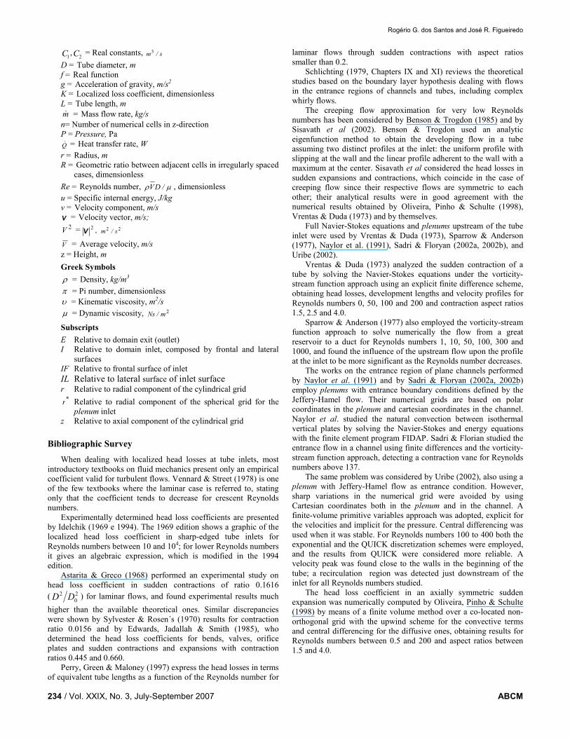
The computational domain is sketched in Fig.1, showing the

physical walls of the tube and the reservoir (full and broken lines) as

well as the fictitious boundaries at the inlet and outlet (dotted lines).

Assuming the flow to be axisymmetric, the cylindrical reference

grid (r,z) is the most appropriate for the numerical computations on

the tube. For geometric simplicity in this reference grid, the plenum

upstream of the tube was established as a cylinder coaxial with the

tube. The spherical reference grid ),r( * θ is useful for analytically

computing the inlet conditions prescribed at the entrance of the

plenum.

Figure 1. Sketch of computational domain, defined by frontal (IF) and lateral (IL) surfaces of the plenum, part of the reservoir wall, tube wall and exit surface (E).

Steady-state incompressible flow with null tangential velocity

was assumed. Constant viscosity and isothermal conditions are also

considered, neglecting the mild effects of the dissipation upon the

thermal state. The governing equations are the continuity and the

Navier-Stokes equations in the following conservative form:

( ) 01

=∂

∂+

∂

∂

z

vvr

rr

zr

(1)

rr

r

rzr

gz

vvr

rrr

r

P

z

vv

r

vr

r

ρµ

ρ

+

∂

∂+

∂

∂

∂

∂+

+∂

∂−=

∂

∂+

∂

∂

2

2

2

)(1

)()(1

(2)

zzz

zzr

gz

v

r

vr

rr

z

P

z

v

r

vvr

r

ρµ

ρ

+

∂

∂+

∂

∂

∂

∂+

+∂

∂−=

∂

∂+

∂

∂

2

2

2

1

)()(1

(3)

The positions of the boundaries at the inlet and outlet of the

domain are somewhat arbitrary. For the exit boundaries, the

numerical tube size was fixed as twice the development size

established by Shah & London (1978) for each Reynolds number

considered. The numerical solution obtained confirmed the

sufficiency of this choice of length.

Domain inlet conditions are generally more influential on the

flow than the outlet conditions, particularly for convection-

dominated flows, and there is no previous estimation of the required

length of the plenum upstream the tube inlet. Arbitrarily setting the

plenum length equal to its radius, a series of preliminary tests

indicated that the profile at the tube entrance turned almost

independent on the plenum size if the plenum radius was at least five

times the tube radius; these proportions were adopted for all cases.

This question is linked to the profile imposed at the plenum

entrance. In the present approach, the domain entrance and exit

boundaries are specified in terms of velocities. Null derivatives were

specified at the exit. The inlet conditions are of specified value, and

two approaches were comparatively employed, each associated to a

distinct model of the flow approaching the tube inlet, interpreted as

a sink for the plenum flow. Both models assumed spherically radial

flows towards the center of the tube inlet, so that the radial velocity

is set in any case as 2*

rr)(fv * θ= . One model considers the

uniform radial flow, which is a classic inviscid solution defined by

1C)(f =θ , slipping on the reservoir walls. The other model emerges

from a creeping flow solution that gives )2cos1()( 2 θθ += Cf ,

obeying the non-slip condition at these walls. The constants 1C and

2C are fixed in terms of the desired Reynolds number, as shown in

detail by Santos (2004). The velocities to be imposed at the plenum

entrance are computed on the spherical reference coordinates and

subsequently projected onto the plenum cylindrical coordinates. As

will be seen, both models produced practically the same profile at

the tube inlet, with minor differences with respect to head loss.

For computing the head loss due to the sharp entrance, one

applies the first law of Thermodynamics to the control volume

defined by the numerical domain, obtaining:

∫ ∫

∫∫

++−=

=

++−

++−

I E

EI

duduQ

dP

gzV

dP

gzV

AVAV

AVAV

ρρ

ρρ

ρρ

&

22

22

(4)

As usual, the vector elementary area Ad is directed outwards the

domain. The left member of the above equation shows the head loss

as the difference between the sums of kinetic, potential and pressure

energies at the inlet and at the outlet of the domain, expressing the

destruction of these thermodynamically noble forms of energy. The

right member represents the same head loss as the thermal energy it

turns into, i.e., either as increased internal energy or as heat

transferred to the surroundings. These thermal forms of energy are

unimportant for the incompressible case. Instead, the head loss is

computed as the sum of distributed and localized losses, as can be

found in any standard textbook in fluid mechanics (see, for instance,

Fox & McDonald, 1988), yielding:

+=

=

++−

++− ∫∫

22

64

22

22

22

EE

EI

VK

V

D

L

Rem

dP

gzV

dP

gzV

&

AVAV ρρ

ρρ (5)

The first term within the parenthesis on the right side of Eq. (5)

corresponds to the distributed loss for the laminar case, and the

second term to the localized loss at the tube inlet. Solving Eq. (5) for

the localized loss coefficient K one obtains:

122

644−

−=υ

πρ

EE VD

LB

VmK

&

where B is an auxiliary parameter given by:

Rogério G. dos Santos and José R. Figueiredo

/ Vol. XXIX, No. 3, July-September 2007 ABCM 236

drrvP

gzV

drrvP

gzV

dzvP

gzV

rB

zE

zIFrILIL

∫

∫∫

++−

+++

++=

ρ

ρρ

2

22

2

22

(7)

The squared velocity module 2

2 VVr

= is computed as the sum

of the squared velocity components )( 22zr vv + . The above

integrations are performed numerically after the converged solution

is found, for various grid refinement levels. The final coefficient is

obtained by means of the Richardson’s extrapolation for vanishing

grid sizes.

Numerical Solution

The numerical problem was solved employing the proprietary

CFD code PHOENICS, which operates with primitive variables

using the SIMPLEST procedure to relate the pressure and the

continuity equation.

The numerical grid was regular in the r-coordinate on the whole

domain and also regular in the z-coordinates within the plenum. For

lower Reynolds numbers, where the developed profile is achieved in

short distances, the grid was also regular in the tube, with the same

spacing used in the plenum. Only for Reynolds numbers of 20 and

above 20, that required large tube sizes to achieve the developed

profile, was it found advantageous to employ irregular grids in the z-

coordinate within the tube, so decreasing the number of cells. In

these cases, the first cell in the tube had the same size of the cells in

the plenum and the remaining cell sizes in the tube were set

geometrically crescent.

The code also offers another grid size variation rule, called

power rule, which was avoided because it leads to cells sizes

varying, in relative terms, very strongly in the beginning of the tube

and very smoothly afterwards, while the geometric rule imposes a

uniform rate of variation across the space.

In order to keep the same convergence characteristics of the

regularly spaced case, the refinement studies used the cell size

geometric ratio R decreasing with the number of z-direction cells n

in such a way that the product n ln R was kept constant. This

criterion was inspired by Rivas’ (1972) demonstration that the

quadratic spatial convergence of the central differencing scheme is

maintained for irregular grids, provided that during the refinement

process there is a unique function with bounded non-null derivatives

mapping a regularly spaced transformed domain into the irregularly

spaced physical domain. The above referred criterion was shown to

hold for many other quadratic discretization schemes by a simple

numerical test due to Figueiredo and Llagostera (2000, also

Llagostera and Figueiredo, 2000).

The last decades saw extensive research on numerical

discretization schemes for the momentum equations and other

convective-diffusive transport equations. So far, central differencing

remains a sufficiently accurate scheme if it is stable, and, for high

Reynolds numbers, the QUICK scheme emerges as one of the most

successful. This conclusion was confirmed for entrance flows in

channels by Uribe (2002).

The UNIFAES scheme (Figueiredo, 1997) has shown generally

superior accuracy, and always superior stability and robustness in

comparison with both central differencing and QUICK (Vilela,

2001). However, while central differencing and QUICK are

incorporated, together with other schemes, to the PHOENICS code,

the new scheme UNIFAES has not been implemented in any

commercial code so far.

Accordingly, the present computations employed the central

differencing scheme for Reynolds numbers up to 100. The QUICK

scheme for Reynolds numbers of 100 and above, where the central

differencing did not converge. Very close results were obtained with

the two schemes for the common case of Reynolds number equal to

100.

The convergence criteria in each case was such that the result is

not affected by lower levels of tolerance.

Results

Fig. 2 shows the axial and radial velocity component profiles

obtained at the tube entrance assuming both inviscid and creeping

flows at the plenum inlet for Reynolds number equal to 100. The

two profiles are visually identical for both boundary conditions, in a

clear indication that the plenum size is sufficient.

Figure 2. Axial and radial velocity components on east plenum entrance for Re=100.

Figure 3. Axial velocity profiles at tube inlet for Re between 20 and 200.

Figure 4. Radial velocity profiles at tube inlet for Re between 20 and 200.

Laminar Elliptic Flow in the Entrance Region of Tubes

J. of the Braz. Soc. of Mech. Sci. & Eng. Copyright 2007 by ABCM July-September 2007, Vol. XXIX, No. 3 / 237

Figure 5. Axial velocity profiles at tube inlet for Re between 200 and 2000.

Figure 6. Radial velocity profiles at tube inlet for Re between 200 and 2000.

Figure 7. Developing axial velocity profiles for Re=200.

Figure 8. Developing radial velocity profiles for Re=200.

Figure 9. Developing axial velocity profiles for Re=2000.

Figure 10. Developing radial velocity profiles for Re=2000.

Figures 3 to 6 show the evaluation of the inlet profile for

variable Reynolds numbers. For Reynolds numbers greater than

100, the axial velocity component develops a peak that becomes

more pronounced and closer to the tube wall as the Reynolds

number increases. The radial velocity component also develops a

negative peak in about same place, and its magnitude reaches about

half the magnitude of the axial velocity, showing that it is by no

means negligible as the parallel flow assumes.

The evolution of the velocity profiles along the tube is shown in

Fig. 7 to 10 for Reynolds numbers 200 and 2000. For Re=200 the

initial peak velocity has entirely disappeared at the distance of 1D

from the entrance, while for Re=2000 a distance equivalent to 3D

was necessary. For Reynolds number 2000, as well as for 1000, a

recirculating zone is detected in the entrance.

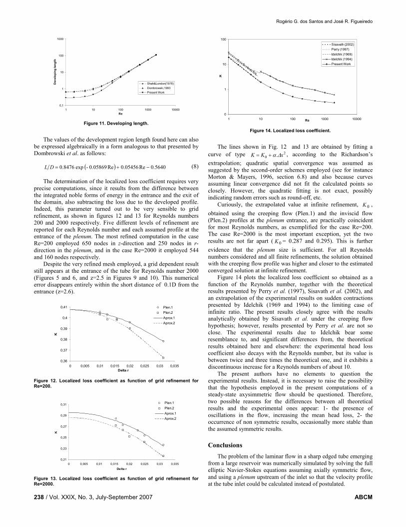
The length of the developing region, defined as the distance

from the tube inlet to the point where the centerline velocity

achieves 99% of its developed value, is plotted in Fig. 11 for

varying Reynolds numbers, together with the developing lengths

obtained by Shah & London (1978) and by Dombrowki et al. (1993)

using the parabolic model. Clearly, all results are very similar for

moderate and high Reynolds numbers, and differ sensibly for low

Reynolds numbers, representing creeping and other flow situations

where the parabolic model is not applicable.

Rogério G. dos Santos and José R. Figueiredo

/ Vol. XXIX, No. 3, July-September 2007 ABCM 238

0,1

1

10

100

1000

1 10 100 1000 10000

Re

Developing length

Shah&London(1978)

Dombrowski,1993

Present Work

Figure 11. Developing length.

The values of the development region length found here can also

be expressed algebraically in a form analogous to that presented by

Dombrowski et al. as follows:

( ) 5640.0Re05456.0Re0.05869-exp8476.0 −+=DL (8)

The determination of the localized loss coefficient requires very

precise computations, since it results from the difference between

the integrated noble forms of energy in the entrance and the exit of

the domain, also subtracting the loss due to the developed profile.

Indeed, this parameter turned out to be very sensible to grid

refinement, as shown in figures 12 and 13 for Reynolds numbers

200 and 2000 respectively. Five different levels of refinement are

reported for each Reynolds number and each assumed profile at the

entrance of the plenum. The most refined computation in the case

Re=200 employed 650 nodes in z-direction and 250 nodes in r-

direction in the plenum, and in the case Re=2000 it employed 544

and 160 nodes respectively.

Despite the very refined mesh employed, a grid dependent result

still appears at the entrance of the tube for Reynolds number 2000

(Figures 5 and 6, and z=2.5 in Figures 9 and 10). This numerical

error disappears entirely within the short distance of 0.1D from the

entrance (z=2.6).

0,36

0,37

0,38

0,39

0,4

0,41

0 0,005 0,01 0,015 0,02 0,025 0,03 0,035

Delta r

K

Plen.1

Plen.2

Aprox.1

Aprox.2

Figure 12. Localized loss coefficient as function of grid refinement for Re=200.

0,21

0,23

0,25

0,27

0,29

0,31

0 0,005 0,01 0,015 0,02 0,025 0,03 0,035

Delta r

K

Plen.1

Plen.2

Aprox.1

Aprox.2

Figure 13. Localized loss coefficient as function of grid refinement for Re=2000.

0

1

10

100

1 10 100 1000 10000Re

K

Sisavath (2002)

Perry (1997)

Idelchik (1969)

Idelchik (1994)

Present Work

Figure 14. Localized loss coefficient.

The lines shown in Fig. 12 and 13 are obtained by fitting a

curve of type 20 . xKK ∆α+= , according to the Richardson’s

extrapolation; quadratic spatial convergence was assumed as

suggested by the second-order schemes employed (see for instance

Morton & Mayers, 1996, section 6.8) and also because curves

assuming linear convergence did not fit the calculated points so

closely. However, the quadratic fitting is not exact, possibly

indicating random errors such as round-off, etc.

Curiously, the extrapolated value at infinite refinement, 0K ,

obtained using the creeping flow (Plen.1) and the inviscid flow

(Plen.2) profiles at the plenum entrance, are practically coincident

for most Reynolds numbers, as exemplified for the case Re=200.

The case Re=2000 is the most important exception, yet the two

results are not far apart ( 0K = 0.287 and 0.295). This is further

evidence that the plenum size is sufficient. For all Reynolds

numbers considered and all finite refinements, the solution obtained

with the creeping flow profile was higher and closer to the estimated

converged solution at infinite refinement.

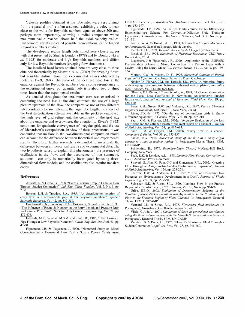
Figure 14 plots the localized loss coefficient so obtained as a

function of the Reynolds number, together with the theoretical

results presented by Perry et al. (1997), Sisavath et al. (2002), and

an extrapolation of the experimental results on sudden contractions

presented by Idelchik (1969 and 1994) to the limiting case of

infinite ratio. The present results closely agree with the results

analytically obtained by Sisavath et al. under the creeping flow

hypothesis; however, results presented by Perry et al. are not so

close. The experimental results due to Idelchik bear some

resemblance to, and significant differences from, the theoretical

results obtained here and elsewhere: the experimental head loss

coefficient also decays with the Reynolds number, but its value is

between twice and three times the theoretical one, and it exhibits a

discontinuous increase for a Reynolds numbers of about 10.

The present authors have no elements to question the

experimental results. Instead, it is necessary to raise the possibility

that the hypothesis employed in the present computations of a

steady-state axysimmetric flow should be questioned. Therefore,

two possible reasons for the differences between all theoretical

results and the experimental ones appear: 1- the presence of

oscillations in the flow, increasing the mean head loss, 2- the

occurrence of non symmetric results, occasionally more stable than

the assumed symmetric results.

Conclusions

The problem of the laminar flow in a sharp edged tube emerging

from a large reservoir was numerically simulated by solving the full

elliptic Navier-Stokes equations assuming axially symmetric flow,

and using a plenum upstream of the inlet so that the velocity profile

at the tube inlet could be calculated instead of postulated.

Laminar Elliptic Flow in the Entrance Region of Tubes

J. of the Braz. Soc. of Mech. Sci. & Eng. Copyright 2007 by ABCM July-September 2007, Vol. XXIX, No. 3 / 239

Velocity profiles obtained at the tube inlet were very distinct

from the parallel profile often assumed, exhibiting a velocity peak

close to the walls for Reynolds numbers equal or above 200 and,

perhaps more importantly, showing a radial component whose

maximum value reaches about half the axial velocity values.

Furthermore, results indicated possible recirculations for the highest

Reynolds numbers studied.

The developing region length determined here closely agrees

with that presented by Shah & London (1978) and by Dombrowki et

al. (1993) for moderate and high Reynolds numbers, and differs

only for low Reynolds numbers (creeping flow situations).

The localized head losses obtained here are very close to those

obtained theoretically by Sisavath et al. (2002) for creeping flows,

but sensibly distinct from the experimental values obtained by

Idelchik (1969, 1994). The curve of the localized head loss at the

entrance against the Reynolds numbers bears some resemblance to

the experimental curve, but quantitatively it is about two or three

times lower than the experimental results.

As detailed throughout the text, much care was exercised in

computing the head loss at the duct entrance: the use of a large

plenum upstream of the flow, the comparative use of two different

inlet conditions for such plenum, the large tube length, the choice of

the best discretization scheme available in the package employed,

the high level of grid refinement, the continuity of the grid size

about the entrance and everywhere, the attention to Rivas´s (1972)

conditions for quadratic convergence of irregular grid, and the use

of Richardson’s extrapolation. In view of these precautions, it was

concluded that no flaw in the two-dimensional computation model

can account for the difference between theoretical and experimental

results. Therefore, further research is demanded to investigate the

difference between all theoretical results and experimental data. The

two hypothesis raised to explain this phenomena - the presence of

oscillations in the flow, and the occurrence of non symmetric

solutions - can only be numerically investigated by using three-

dimensional flow models, and the oscillations also require transient

codes.

References

Astarita, G. & Greco, G., 1968, “Excess Pressure Drop in Laminar Flow Through Sudden Contraction”, Ind. Eng. Chem. Fundam, Vol. 7, No. 1, pp. 27-31.

Benson, L.H. & Trogdon, S.A., 1985, “An eigenfunction solution of entry flow in a semi-infinite pipe at low Reynolds numbers”, Applied Scientific Research, Vol. 42, pp. 347-359.

Dombrowski, N., Foumeny, E.A., Ookawara, S. and Riza, A., 1993, “The Influence of Reynolds Number on the Entry Length and Pressure Drop for Laminar Pipe Flow”, The Can. J. of Chemical Engineering, Vol. 71, pp. 472-476.

Edwards, M.F., Jadallah, M.S.M. and Smith, R., 1985, “Head Losses in Pipe Fittings at Low Reynolds Numbers”, Chem. Eng. Res. Des.,Vol. 63, pp. 43-50.

Figueiredo, J.R. & Llagostera, J., 2000, “Numerical Study on Mixed Convection in a Horizontal Flow Past a Square Porous Cavity using

UNIFAES Scheme”, J. Brazilian Soc. Mechanical Sciences, Vol. XXII, No. 4, pp. 583-597.

Figueiredo, J.R., 1997, “A Unified Finite-Volume Finite-Differencing Exponential-type Scheme For Convective-Diffusive Fluid Transport Equations”, J. Brazilian Soc. Mechanical Sciences, Vol. XIX, No. 3, pp. 371-391.

Fox. R. W. & McDonald, A. T., 1988, Introduction to Fluid Mechanics (in Portuguese), Guanabara Koogan, Rio de Janeiro.

Idelchick, I.E., 1969, Memento des Pertes de Charge Eyrolles, Paris. Idelchick, I.E., 1994, Handbook of Hydraulic Resistance, CRC Press,

Boca Raton, 3rd ed. Llagostera, J & Figueiredo, J.R., 2000, “Application of the UNIFAES

Discretization Scheme to Mixed Convection in a Porous Layer with a Cavity, Using the Darcy Model”, J. Porous Media, Vol. 3, No. 2, pp. 139-154.

Morton, K.W. & Mayers, D. F., 1996, Numerical Solution of Partial Differential Equations, Cambrige University Press, Cambridge

Naylor, D., Floryan, J.M. and Tarasuk, J.D., 1991, “A numerical Study of developing free convection between isothermal vertical plates”, Journal of Heat Transfer, Vol. 113, pp. 620-626.

Oliveira, P.J., Pinho, F.T and Schulte, A., 1998, “A General Correlation for the Local Loss Coefficient in Newtoniam Axisymmetric Sudden Expansions”, International Journal of Heat and Fluid Flow, Vol. 19, pp. 655-660

Perry, R.H., Green, D.W. and Maloney, J.O., 1997, Perry’s Chemical Engineers’Handbook, McGraw-Hill, New York, 7th ed.

Rivas, E.K de, 1972, “On the use of non-uniform grids in finite-difference equations”, J. Comput. Phys., Vol. 10, pp. 202-210.

Sadri, R.M. & Floryan, J.M., 2002a, “Accurate Evaluation of the loss coefficient and the entrance length of the inlet region of a channel”, Journal of Fluids Engineering, Vol.124, pp. 685-693.

Sadri, R.M. & Floryan, J.M., 2002b, “Entry flow in a chanel” Computers & Fluids, Vol. 31, pp. 133-137.

Santos, R.G., 2004, Numerical Study of the flow at a sharp-edged entrace to a pipe in laminar regime (in Portuguese) Master Thesis, FEM, UNICAMP.

Schlichting, H., 1979, Boundary-Layer Theory, McGraw-Hill Book Company, New York.

Shah, R.K. & London, A.L., 1978, Laminar Flow Forced Convection in Ducts, Academic Press, New York.

Sisavath, S., Jing, X., Pain, C.C. and Zinnerman, R.W., 2002, “Creeping Flow Through an Axisymmetric Sudden Contracrion or Expansion”, Journal of Fluids Engineering, Vol. 124, pp. 273-278.

Sparrow, E.W. & Anderson, C.E., 1977, “Effect of Upstream Flow Processes on Hydrodynamic Development in a Duct”, Journal of Fluids Engineering, Vol. 99, pp. 556-560.

Sylvester, N.D. & Rosen, S.L., 1970, “Laminar Flow in the Entrace Region of a Circular Tube”, AIChE Journal, Vol. 16, No. 6, pp. 964-971.

Uribe, E.B.O., 2002, Evaluation of Discretization Schemes in the Solution of Navier-Stokes Equations and Application to the Problem of the Flow in the Entrance Region of Plane Channels (in Portuguese), Doctoral Thesis, FEM, UNICAMP.

Vennard, J.K. & Street, R.L., 1978, Elementary fluid mechanics (in Portuguese), Guanabara Dois, Rio de Janeiro, 5th ed.

Vilela, C.A.deA., 2001, Simulation of flows in generalized coordinates using the finite volume method with the UNIFAES discretization scheme (in Portuguese), Doctoral Thesis, FEM, UNICAMP.

Vrentas, J.S. & Duda, J.L., 1973, “Flow of a Newtonian Fluid Through a Sudden Contraction”, Appl. Sci. Res., Vol. 28, pp. 241-260.