eScholarship provides open access, scholarly publishingservices to the University of California and delivers a dynamicresearch platform to scholars worldwide.

University of California

Peer Reviewed

Title:Computational vascular fluid–structure interaction: methodology and application to cerebralaneurysms

Author:Bazilevs, Y.; Hsu, M.-C.; Zhang, Y.; Wang, W.; Kvamsdal, T.; Hentschel, S.; et al.

Publication Date:2010

Publication Info:Postprints, UC San Diego

Permalink:http://escholarship.org/uc/item/6x41w0fw

DOI:10.1007/s10237-010-0189-7

Abstract:A computational vascular fluid–structure interaction framework for the simulation of patient-specific cerebral aneurysm configurations is presented. A new approach for the computation ofthe blood vessel tissue prestress is also described. Simulations of four patient-specific models arecarried out, and quantities of hemodynamic interest such as wall shear stress and wall tensionare studied to examine the relevance of fluid–structure interaction modeling when compared tothe rigid arterial wall assumption. We demonstrate that flexible wall modeling plays an importantrole in accurate prediction of patient-specific hemodynamics. Discussion of the clinical relevanceof our methods and results is provided.

Biomech Model Mechanobiol (2010) 9:481–498DOI 10.1007/s10237-010-0189-7

ORIGINAL PAPER

Computational vascular fluid–structure interaction: methodologyand application to cerebral aneurysms

Y. Bazilevs · M.-C. Hsu · Y. Zhang · W. Wang ·T. Kvamsdal · S. Hentschel · J. G. Isaksen

Received: 13 April 2009 / Accepted: 11 January 2010 / Published online: 29 January 2010© The Author(s) 2010. This article is published with open access at Springerlink.com

Abstract A computational vascular fluid–structure interac-tion framework for the simulation of patient-specific cerebralaneurysm configurations is presented. A new approach forthe computation of the blood vessel tissue prestress is alsodescribed. Simulations of four patient-specific models arecarried out, and quantities of hemodynamic interest such aswall shear stress and wall tension are studied to examine therelevance of fluid–structure interaction modeling when com-pared to the rigid arterial wall assumption. We demonstratethat flexible wall modeling plays an important role in accurateprediction of patient-specific hemodynamics. Discussion ofthe clinical relevance of our methods and results is provided.

Y. Bazilevs (B) · M.-C. HsuDepartment of Structural Engineering, University of California,San Diego, 9500 Gilman Drive, La Jolla, CA 92093, USAe-mail: yuri@ucsd.edu

Y. Zhang · W. WangDepartment of Mechanical Engineering, Carnegie MellonUniversity, Pittsburgh, PA 15213, USA

T. KvamsdalDepartment of Applied Mathematics, SINTEF Informationand Communication Technology,7465 Trondheim, Norway

S. HentschelDepartment of Scientific Computing, Simula,Martin Linges vei 17, 1364 Fornebu, Norway

J. G. IsaksenDepartments of Neurosurgery and Neurology, University Hospitalof North Norway, 9038 Tromsø, Norway

J. G. IsaksenInstitute of Clinical Medicine, University of Tromsø,9037 Tromsø, Norway

Keywords Cerebral aneurysms · Fluid–structureinteraction · Arterial wall tissue modeling · IncompressibleNavier–Stokes equations · Boundary layer meshing ·Wall shear stress · Wall tension · Tissue prestress

1 Introduction

Starting with a pioneering work on patient-specific vascularmodeling in Taylor et al. (1998), the field of computa-tional vascular and cardiovascular modeling has maturedimmensely over the last decade. Numerous advances inthe simulation technology were proposed, such as imposi-tion of physiologically-realistic outflow boundary conditions(Formaggia et al. 2001; Lagana et al. 2002; Vignon-Clementel et al. 2006), simulation of stenting technologyin the context of cerebral aneurysms (Appanaboyina et al.2009) and coronary arteries (Zunino et al. 2009), optimi-zation of cardiovascular geometries for surgical treatment(Marsden et al. 2008), inclusion of the effects of wall elastic-ity (Figueroa et al. 2006; Bazilevs et al. 2006, 2008; Tezduyaret al. 2007; Torii et al. 2008, 2009), and growth and remod-eling (Figueroa et al. 2009) in the simulations. Nowadays,the state-of-the-art in computational hemodynamics involvesfully coupled fluid–structure patient-specific simulations oflarge portions of the human cardiovascular system. Simula-tions are performed in an effort to investigate hemodynamicfactors influencing the onset and progression of cardiovascu-lar disease, to predict an outcome of a surgical intervention,or to evaluate the effects of electromechanical assist devices.

Currently, assessment of aneurysm rupture risk is basedon known risk factors like smoking, hypertension, family his-tory of subarachnoid hemorrhage, and aneurysm size, derivedfrom epidemiological and clinical studies. However, the cur-rent knowledge is not sufficient for patient-specific clinical

123

482 Y. Bazilevs et al.

decision-making. Recently, the aneurysm shape was pro-posed as an important, patient-specific, independent rupturerisk factor (Aneurysm Registry of Helsinki 2009; AneurysmRegistry of Tromsø 2009; Frösen J. Private communication2009). As a result, in recent years, a considerable effort wasput forth to apply pure computational fluid dynamics (CFD)techniques to study and classify flow patterns and wall shearstress (WSS) and oscillatory shear index (OSI) distributionsin a large sample of patient-specific cerebral aneurysm shapes(see, e.g., Sforza et al. 2009 and references therein). Thesequantities of hemodynamic interest, practically unattainablein experiments or measurements, are connected to clinicalevents, which help better understand the disease processesand improve patient evaluation and treatment.

When pure CFD is used for vascular blood flow sim-ulations, it is assumed that the vessel wall remains rigid.The rigid wall assumption does not properly reflect thebehavior of real blood vessels that deform under the actionof blood flow forces and, in turn, alter the details ofblood flow. For the modeling to be realistic, coupled fluid–structure interaction (FSI) modeling must be employed.However, high-fidelity FSI of vascular blood flow in apatient-specific setting is scarce, which is mainly due tothe numerical challenges involved. Despite its modelingshortcomings, pure CFD remains the predominant modelingapproach for vascular blood flow, and, in particular, for com-putation of aneurysm flows. Notable exceptions include thework of (Takizawa et al. 2010a,b; Torii et al. 2006a,b, 2007,2008, 2009) on cerebral aneurysms and the work of (Wolterset al. 2005; Scotti and Finol 2007; Rissland et al. 2009) onaortic abdominal aneurysms. This paper likewise focuseson developing and using advanced FSI computational tech-niques to assess the risk of rupture for cerebral aneurysmsin individual patients. Our FSI framework involves the cou-pling of incompressible fluid representing the blood and ahyperelastic solid representing vessel wall tissue. The equa-tions are posed on a moving domain and are equipped withan appropriate set of boundary and initial conditions. Vari-able wall thickness, tissue prestress, sliding inlet and outletbranch boundary conditions, and boundary layer meshingare the key ingredients of our computational framework thatallow for physiologically realistic and accurate simulations.It should also be noted that the importance of the problemof cerebral aneurysm rupture and its resolution by meansof advanced numerical simulation was discussed in a recentreview article on open problem in vascular modeling (Taylorand Humphrey 2009).

This paper is outlined as follows. In Sect. 2, we recallthe formulation of the fluid and solid sub-problems andtheir interface conditions that ensure appropriate couplingbetween the two systems. The basic coupled formulationwas developed in Bazilevs et al. (2008) and the modelingis further improved here. We introduce the vessel wall tissue

prestress that was not accounted for in our original mod-eling framework. The need for modeling tissue prestressarises due to the fact that the arterial configuration comingfrom patient-specific imaging data is subjected to intramuralblood pressure and viscous forces. As a result, it may not betaken as a stress-free reference configuration. An approachis presented that circumvents this difficulty by prescribinga state of prestress to the arterial tissue that puts the arteryin equilibrium with the blood flow forces. In Sect. 3, webriefly recall our meshing and basic computational proce-dures for the simulation of arterial fluid–structure interactionphenomena. Patient-specific models are presented, and meshstatistics are summarized. Out of the four patient-specificaneurysm models analyzed, two correspond to ruptured andtwo to unruptured cases. Fine meshes with boundary layerresolution are employed, which ensures high fidelity of thecomputational results. Simulations are driven by a prescribedtime-periodic inlet velocity and outlet resistance boundaryconditions that ensure physiological pressure levels in thevessels. We also introduce free-slip boundary conditions atthe model inlets and outlets. This gives the inlet and outletbranches a flexibility to move in their cut planes as well asdeform radially in response to variations in the intramuralpressure and viscous forces. Free-slip boundary conditionslead to more realistic vessel wall deformations than fixedinlets and outlets that were employed previously. In Sect. 4,we present our simulation results, focusing on the compari-son between rigid and flexible simulations. While the differ-ences in the computed blood flow speeds are not as significant(although clearly visible in some cases), the wall shear stresswas found to be consistently overestimated in the rigid wallsimulations, in one case by as much as 52%, which is felt tobe a significant overestimation. In Sect. 5, we draw conclu-sions and provide discussion of the clinical relevance of ourfindings.

2 Continuum modeling

2.1 Blood flow modeling

The blood flow is governed by the Navier–Stokes equationsof incompressible flow posed on a moving domain. The Arbi-trary Lagrangian–Eulerian (ALE) formulation is used, whichis a widely used approach for vascular blood flow applica-tions (Nobile 2001; Formaggia et al. 2001; Gerbeau et al.2005; Fernández et al. 2008). Alternatively, one can applythe space-time methodology (Tezduyar et al. 2007; Torii et al.2008, 2009), which leads to better time accuracy, yet some-what higher computational expense per time step.

Let V f and W f be the standard solution and weightingfunction spaces for the fluid problem. The variational formu-lation of the Navier–Stokes equations is stated as follows:

123

Computational vascular fluid–structure interaction 483

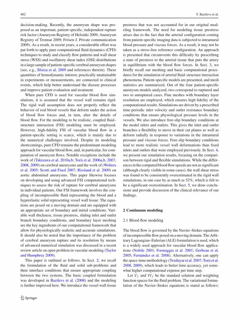
Fig. 1 Dimension, referencegeometry and meshes forModels 1–4 of the middlecerebral artery (MCA)bifurcation. Inlet branches arelabeled M1 and outlet branchesare labeled M2. The arrowspoint in the direction of inflowvelocity

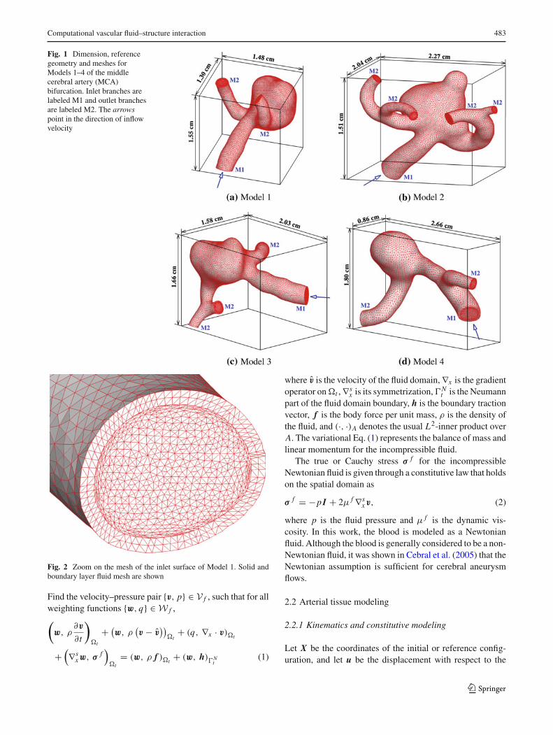
Fig. 2 Zoom on the mesh of the inlet surface of Model 1. Solid andboundary layer fluid mesh are shown

Find the velocity–pressure pair {v, p} ∈ V f , such that for allweighting functions {w, q} ∈ W f ,(

w, ρ∂v

∂t

)�t

+ (w, ρ

(v − v̂

))�t

+ (q, ∇x · v)�t

+(∇s

xw, σ f)

�t= (w, ρ f )�t

+ (w, h)�Nt

(1)

where v̂ is the velocity of the fluid domain, ∇x is the gradientoperator on �t , ∇s

x is its symmetrization, �Nt is the Neumann

part of the fluid domain boundary, h is the boundary tractionvector, f is the body force per unit mass, ρ is the density ofthe fluid, and (·, ·)A denotes the usual L2-inner product overA. The variational Eq. (1) represents the balance of mass andlinear momentum for the incompressible fluid.

The true or Cauchy stress σ f for the incompressibleNewtonian fluid is given through a constitutive law that holdson the spatial domain as

σ f = −p I + 2μ f ∇sxv, (2)

where p is the fluid pressure and μ f is the dynamic vis-cosity. In this work, the blood is modeled as a Newtonianfluid. Although the blood is generally considered to be a non-Newtonian fluid, it was shown in Cebral et al. (2005) that theNewtonian assumption is sufficient for cerebral aneurysmflows.

2.2 Arterial tissue modeling

2.2.1 Kinematics and constitutive modeling

Let X be the coordinates of the initial or reference config-uration, and let u be the displacement with respect to the

123

484 Y. Bazilevs et al.

Table 1 Finite element mesh sizes for the aneurysm models

Model Fluid elements Solid elements Total elements Total nodes

1 407,280 120,000 527,280 94,199

2 341,813 120,684 462,497 83,591

3 232,652 83,598 316,250 57,379

4 96,684 47,928 144,612 26,947

Table 2 Inflow cross-sectional areas for the aneurysm models

Model Inflow surface area (cm2)

1 4.2452 × 10−2

2 9.2985 × 10−2

3 5.6349 × 10−2

4 8.7916 × 10−2

initial configuration. Then, x, the coordinates of the currentconfiguration, is given by

x = X + u. (3)

The deformation gradient tensor F, the Cauchy–Green defor-mation tensor C, and the Green-Lagrangian strain tensor E,are defined as

F = ∂x∂ X

= I + ∂u∂ X

, (4)

C = FT F, (5)

E = 1

2(C − I), (6)

respectively.We model the arterial tissue as a three-dimensional

hyperelastic solid and assume the existence of a stored elasticenergy in the form

ϕ (C, J )= 1

2μs(J−2/3trC−3)+ 1

2κs

(1

2(J 2 − 1)−lnJ

).

(7)

In (7), J = det F, and μs and κs are identified with thematerial shear and bulk moduli, respectively. From (7), thesecond Piola–Kirchhoff stress tensor S and the fourth-ranktensor of material tangent moduli C are obtained as

S = 2∂ϕ

∂C(C, J )

= μs J−2/3(

I − 1

3trC C−1

)+ 1

2κs(J 2 − 1)C−1, (8)

and

Time(s)

Infl

owve

loci

ty(c

m/s

)

0 0.1 0.2 0.3 0.4 0.5 0.6 0.7 0.8 0.9 10

10

20

30

40

50

60

70

Fig. 3 Area-averaged inflow velocity as a function of time during theheart cycle. The inflow velocity profile is taken from Isaksen et al.(2008)

C=4∂2ϕ

∂C∂C(C, J )

=(

2

9μs J−2/3trC+κs J 2

)C−1 ⊗ C−1 (9)

+(

2

3μJ−2/3trC − κs(J 2 − 1)

)C−1 � C−1

−2

3μs J−2/3(I ⊗ C−1 + C−1 ⊗ I). (10)

In (10), the symbols ⊗ and � are defined as

(C−1 ⊗ C−1)I J K L = (C−1)I J (C−1)K L , (11)

(C−1 � C−1)I J K L = (C−1)I K (C−1)J L + (C−1)I L (C−1)J K

2.

(12)

To conclude this section, a few remarks about the proposedsolid model are given.

Remark When the reference and current configurations coin-cide, the expression for the tensor of material tangent moduliC is simplified to

(C)I J K L = (κs − 2

3μs)δI J δK L + μs(δI K δJ L + δI LδJ K ).

(13)

In the above expression, we recognize a tensor of elastic mod-uli for an isotropic, linearly elastic material and interpret μs

and κs as the material shear and bulk moduli, respectively.

Remark The material model is assumed to be isotropic,and the material properties (i.e., the bulk and shear moduli)are chosen from our previous works on cerebral aneurysms(see, e.g., Isaksen et al. 2008). This is an oversimplification,

123

Computational vascular fluid–structure interaction 485

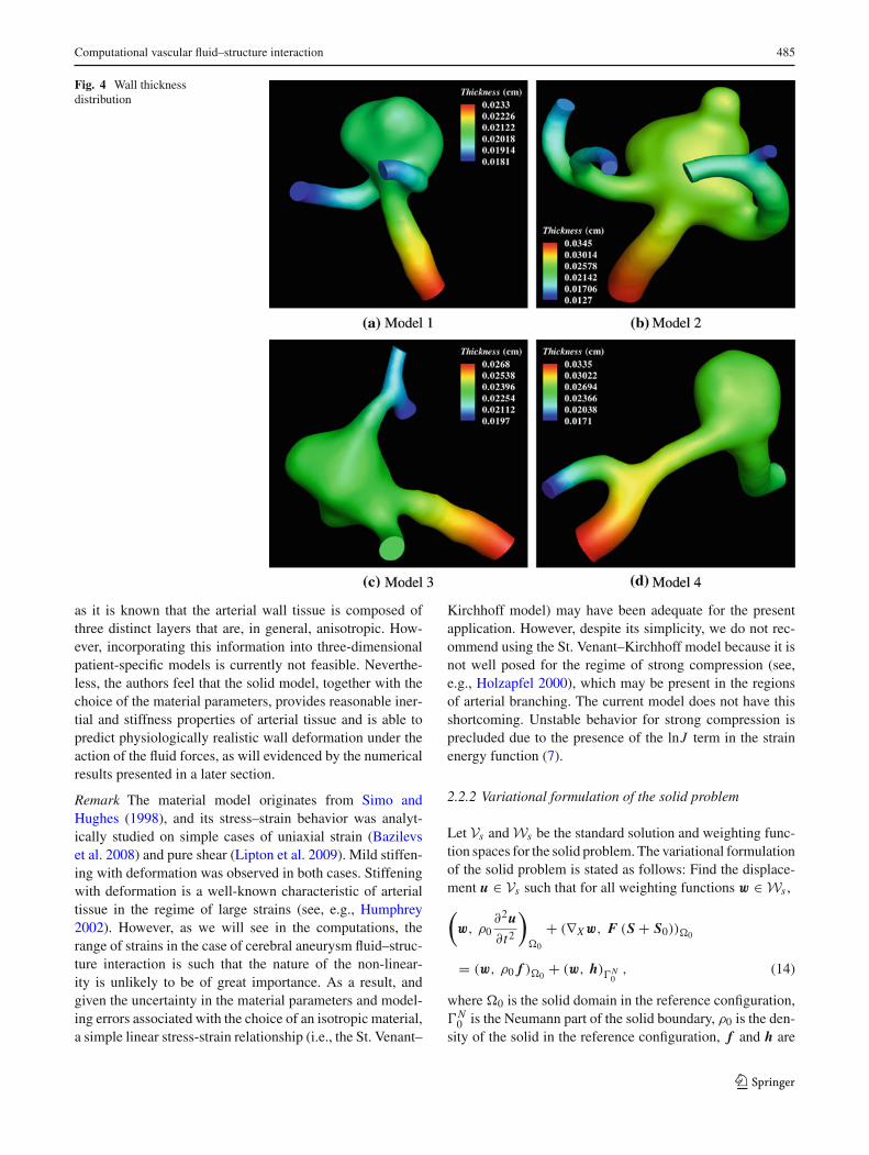
Fig. 4 Wall thicknessdistribution

as it is known that the arterial wall tissue is composed ofthree distinct layers that are, in general, anisotropic. How-ever, incorporating this information into three-dimensionalpatient-specific models is currently not feasible. Neverthe-less, the authors feel that the solid model, together with thechoice of the material parameters, provides reasonable iner-tial and stiffness properties of arterial tissue and is able topredict physiologically realistic wall deformation under theaction of the fluid forces, as will evidenced by the numericalresults presented in a later section.

Remark The material model originates from Simo andHughes (1998), and its stress–strain behavior was analyt-ically studied on simple cases of uniaxial strain (Bazilevset al. 2008) and pure shear (Lipton et al. 2009). Mild stiffen-ing with deformation was observed in both cases. Stiffeningwith deformation is a well-known characteristic of arterialtissue in the regime of large strains (see, e.g., Humphrey2002). However, as we will see in the computations, therange of strains in the case of cerebral aneurysm fluid–struc-ture interaction is such that the nature of the non-linear-ity is unlikely to be of great importance. As a result, andgiven the uncertainty in the material parameters and model-ing errors associated with the choice of an isotropic material,a simple linear stress-strain relationship (i.e., the St. Venant–

Kirchhoff model) may have been adequate for the presentapplication. However, despite its simplicity, we do not rec-ommend using the St. Venant–Kirchhoff model because it isnot well posed for the regime of strong compression (see,e.g., Holzapfel 2000), which may be present in the regionsof arterial branching. The current model does not have thisshortcoming. Unstable behavior for strong compression isprecluded due to the presence of the lnJ term in the strainenergy function (7).

2.2.2 Variational formulation of the solid problem

Let Vs and Ws be the standard solution and weighting func-tion spaces for the solid problem. The variational formulationof the solid problem is stated as follows: Find the displace-ment u ∈ Vs such that for all weighting functions w ∈ Ws ,

(w, ρ0

∂2u∂t2

)�0

+ (∇Xw, F (S + S0))�0

= (w, ρ0 f )�0+ (w, h)�N

0, (14)

where �0 is the solid domain in the reference configuration,�N

0 is the Neumann part of the solid boundary, ρ0 is the den-sity of the solid in the reference configuration, f and h are

123

486 Y. Bazilevs et al.

Fig. 5 Tissue prestress

the body and surface forces, respectively. Variational Eq. (14)represents the balance of linear momentum for the solid.

This formulation is non-standard due to the presence ofthe S0 in the stress term on the left-hand-side of (14). In ourmodeling framework, S0 is a prestress that is present in theartery reference configuration, which is assumed to coincidewith the configuration extracted from patient-specific imag-ing data. This configuration is subjected to blood pressureand viscous forces and, in turn, develops internal stress toresist these loads. This internal stress tensor is denoted byS0, and its computation is presented in the next section.

2.2.3 Blood vessel tissue prestress

The variational formulation of the prestress problem, whichis posed over the same function spaces as the solid problem,is stated as follows: Find the displacement u ∈ Vs such that∀w ∈ Ws ,

(∇Xw, FS)�0+ (w, h)

�f s

0= 0, (15)

where, �f s

0 is the fluid–solid boundary in the reference con-figuration, F and S are defined in Eqs. (4) and (8), respec-

tively, and h is the fluid traction vector consisting of both thepressure and viscous parts, given by

h = σ f n f . (16)

The fluid traction vector may be obtained from a rigid-wallblood flow simulation on a reference domain with steadyinflow and resistance outflow boundary conditions. The lat-ter guarantees a physiological intramural pressure level in thearteries. (For a discussion of outflow boundary conditions forcardiovascular simulations, see, e.g., Vignon-Clementel et al.2006; Bazilevs et al. 2008, 2009a.)

The variational Eq. (15) are solved for the displacementfield u, and the corresponding stress field S is computed fromthe displacement field. The prestress S0 is assigned the valueof S, and the coupled time-dependent fluid–structural prob-lem departs from the prestressed reference configuration withthe initial displacement field set to zero.

Remark Because h is dominated by the intramural pressurepart and the effect of the viscus forces is not as pronounced,one may simplify the definition of the fluid traction vector in(15) to

h = − p̃0n f , (17)

123

Computational vascular fluid–structure interaction 487

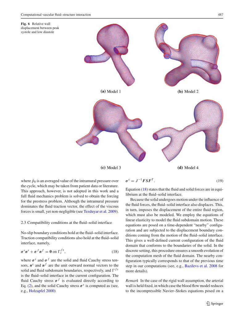
Fig. 6 Relative walldisplacement between peaksystole and low diastole

where p̃0 is an averaged value of the intramural pressure overthe cycle, which may be taken from patient data or literature.This approach, however, is not adopted in this work and afull fluid mechanics problem is solved to obtain the forcingfor the prestress problem. Although the intramural pressuredominates the fluid traction vector, the effect of the viscousforces is small, yet non-negligible (see Tezduyar et al. 2009).

2.3 Compatibility conditions at the fluid–solid interface

No-slip boundary conditions hold at the fluid–solid interface.Traction compatibility conditions also hold at the fluid–solidinterface, namely,

σ s ns + σ f n f = 0 on �f s

t , (18)

where σ s and σ f are the solid and fluid Cauchy stress ten-sors, ns and n f are the unit outward normal vectors to thesolid and fluid subdomain boundaries, respectively, and � f s

is the fluid–solid interface in the current configuration. Thefluid Cauchy stress σ f is evaluated directly according toEq. (2), and the solid Cauchy stress σ s is computed as (see,e.g., Holzapfel 2000)

σ s = J−1 FSFT . (19)

Equation (18) states that the fluid and solid forces are in equi-librium at the fluid–solid interface.

Because the solid undergoes motion under the influence ofthe fluid forces, the fluid–solid interface also displaces. This,in turn, imposes the displacement of the entire fluid region,which must also be modeled. We employ the equations oflinear elasticity to model the fluid subdomain motion. Theseequations are posed on a time-dependent “nearby” configu-ration and are subjected to the displacement boundary con-ditions coming from the motion of the fluid–solid interface.This gives a well-defined current configuration of the fluiddomain that conforms to the boundaries of the solid. In thediscrete setting, this procedure ensures a smooth evolution ofthe computation mesh of the fluid domain. The nearby con-figuration typically corresponds to that of the previous timestep in our computations (see, e.g., Bazilevs et al. 2008 formore details).

Remark In the case of the rigid wall assumption, the arterialwall is held fixed, in which case the blood flow model reducesto the incompressible Navier–Stokes equations posed on a

123

488 Y. Bazilevs et al.

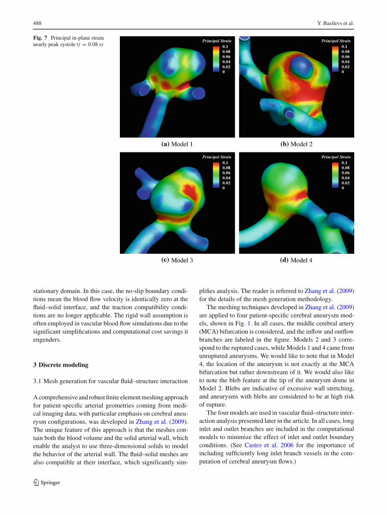
Fig. 7 Principal in-plane strainnearly peak systole (t = 0.08 s)

stationary domain. In this case, the no-slip boundary condi-tions mean the blood flow velocity is identically zero at thefluid–solid interface, and the traction compatibility condi-tions are no longer applicable. The rigid wall assumption isoften employed in vascular blood flow simulations due to thesignificant simplifications and computational cost savings itengenders.

3 Discrete modeling

3.1 Mesh generation for vascular fluid–structure interaction

A comprehensive and robust finite element meshing approachfor patient-specific arterial geometries coming from medi-cal imaging data, with particular emphasis on cerebral aneu-rysm configurations, was developed in Zhang et al. (2009).The unique feature of this approach is that the meshes con-tain both the blood volume and the solid arterial wall, whichenable the analyst to use three-dimensional solids to modelthe behavior of the arterial wall. The fluid–solid meshes arealso compatible at their interface, which significantly sim-

plifies analysis. The reader is referred to Zhang et al. (2009)for the details of the mesh generation methodology.

The meshing techniques developed in Zhang et al. (2009)are applied to four patient-specific cerebral aneurysm mod-els, shown in Fig. 1. In all cases, the middle cerebral artery(MCA) bifurcation is considered, and the inflow and outflowbranches are labeled in the figure. Models 2 and 3 corre-spond to the ruptured cases, while Models 1 and 4 came fromunruptured aneurysms. We would like to note that in Model4, the location of the aneurysm is not exactly at the MCAbifurcation but rather downstream of it. We would also liketo note the bleb feature at the tip of the aneurysm dome inModel 2. Blebs are indicative of excessive wall stretching,and aneurysms with blebs are considered to be at high riskof rupture.

The four models are used in vascular fluid–structure inter-action analysis presented later in the article. In all cases, longinlet and outlet branches are included in the computationalmodels to minimize the effect of inlet and outlet boundaryconditions. (See Castro et al. 2006 for the importance ofincluding sufficiently long inlet branch vessels in the com-putation of cerebral aneurysm flows.)

123

Computational vascular fluid–structure interaction 489

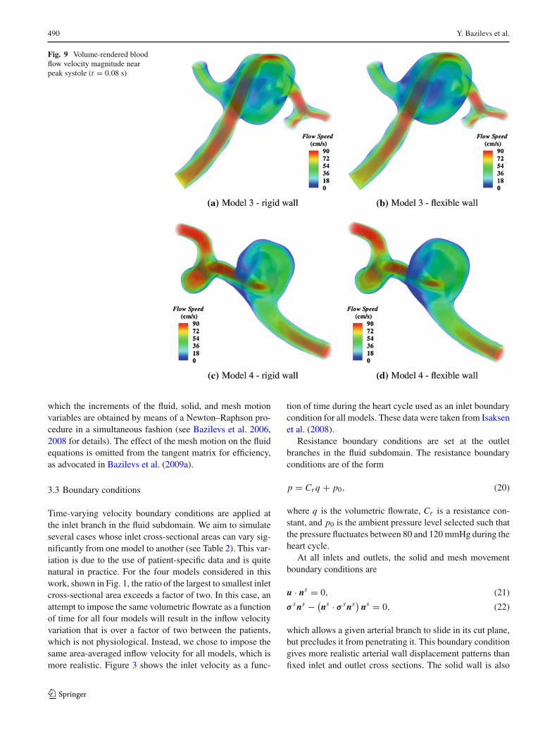
Fig. 8 Volume-rendered bloodflow velocity magnitude nearpeak systole (t = 0.08 s)

The meshes for both fluid and solid regions consist of lin-ear tetrahedral elements, and the solid wall is meshed usingtwo layers of elements in the through-thickness direction.The choice of tetrahedral over hexahedral discretization ismotivated by the relative simplicity of the former approachwith respect to the latter for meshing of complex geometri-cal configurations. Boundary layer meshing is employed inthe fluid region to enhance the resolution of wall quantities,such as the shear stress. Figure 2 zooms on the inlet branchof Model 1 where one can clearly see the solid wall and thehigh-quality boundary layer fluid mesh. The meshes for theremaining three models are of similar quality.

Mesh sizes for all models are summarized in Table 1. Thelocal element Reynolds number based on the mean bloodflow speed during the heart cycle is about 10 in the domaininterior and decreases to about 1.5 near the solid wall dueto boundary layer meshing. The proposed numerical meth-odology used for the fluid mechanics problem, discussed inthe sequel, is known to deliver accurate prediction of flowphenomena for this range of Reynolds numbers, on both tet-rahedral and hexahedral discretizations. On a related note, ina recent study (Takizawa et al. 2010b), the authors showedthat the quantities of hemodynamic interest, such as the wall

shear stress, are accurately represented for cerebral aneurysmflows at the level of mesh resolution employed in this work.

3.2 Discretization and solution strategies

The solid and fluid mesh motion equations are discret-ized using the Galerkin approach. The fluid formulationmakes use of the recently proposed residual-based variationalmultiscale method (Bazilevs et al. 2007). The residual-basedvariational multiscale methodology is built on the theory ofstabilized and multiscale methods (see Brooks and Hughes1982 for an early reference; Hughes et al. 2004 for a com-prehensive review; and Tezduyar 2003; Bazilevs et al. 2007for specific expressions employed in the definition of stabil-ization parameters). The methodology applies equally wellto laminar and turbulent flows and is thus attractive for appli-cations where the nature of the flow solution is not knowna priori. The time-dependent discrete equations are solvedusing the generalized-α time integrator proposed in Chungand Hulbert (1993) for the equations of structural mechan-ics, developed in Jansen et al. (1999) for fluid dynamics,and further extended in Bazilevs et al. (2008) to fluid–struc-ture interaction. A monolithic solution strategy is adopted in

123

490 Y. Bazilevs et al.

Fig. 9 Volume-rendered bloodflow velocity magnitude nearpeak systole (t = 0.08 s)

which the increments of the fluid, solid, and mesh motionvariables are obtained by means of a Newton–Raphson pro-cedure in a simultaneous fashion (see Bazilevs et al. 2006,2008 for details). The effect of the mesh motion on the fluidequations is omitted from the tangent matrix for efficiency,as advocated in Bazilevs et al. (2009a).

3.3 Boundary conditions

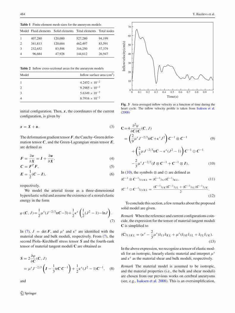
Time-varying velocity boundary conditions are applied atthe inlet branch in the fluid subdomain. We aim to simulateseveral cases whose inlet cross-sectional areas can vary sig-nificantly from one model to another (see Table 2). This var-iation is due to the use of patient-specific data and is quitenatural in practice. For the four models considered in thiswork, shown in Fig. 1, the ratio of the largest to smallest inletcross-sectional area exceeds a factor of two. In this case, anattempt to impose the same volumetric flowrate as a functionof time for all four models will result in the inflow velocityvariation that is over a factor of two between the patients,which is not physiological. Instead, we chose to impose thesame area-averaged inflow velocity for all models, which ismore realistic. Figure 3 shows the inlet velocity as a func-

tion of time during the heart cycle used as an inlet boundarycondition for all models. These data were taken from Isaksenet al. (2008).

Resistance boundary conditions are set at the outletbranches in the fluid subdomain. The resistance boundaryconditions are of the form

p = Cr q + p0, (20)

where q is the volumetric flowrate, Cr is a resistance con-stant, and p0 is the ambient pressure level selected such thatthe pressure fluctuates between 80 and 120 mmHg during theheart cycle.

At all inlets and outlets, the solid and mesh movementboundary conditions are

u · ns = 0, (21)

σ s ns − (ns · σ s ns) ns = 0, (22)

which allows a given arterial branch to slide in its cut plane,but precludes it from penetrating it. This boundary conditiongives more realistic arterial wall displacement patterns thanfixed inlet and outlet cross sections. The solid wall is also

123

Computational vascular fluid–structure interaction 491

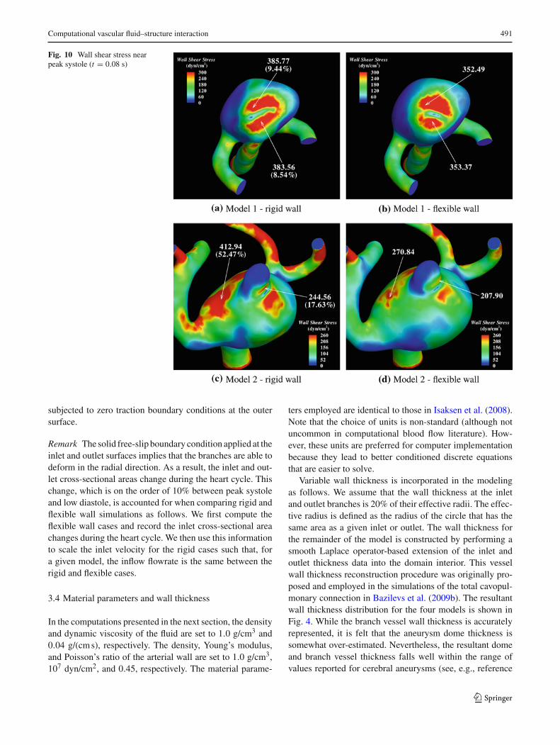
Fig. 10 Wall shear stress nearpeak systole (t = 0.08 s)

subjected to zero traction boundary conditions at the outersurface.

Remark The solid free-slip boundary condition applied at theinlet and outlet surfaces implies that the branches are able todeform in the radial direction. As a result, the inlet and out-let cross-sectional areas change during the heart cycle. Thischange, which is on the order of 10% between peak systoleand low diastole, is accounted for when comparing rigid andflexible wall simulations as follows. We first compute theflexible wall cases and record the inlet cross-sectional areachanges during the heart cycle. We then use this informationto scale the inlet velocity for the rigid cases such that, fora given model, the inflow flowrate is the same between therigid and flexible cases.

3.4 Material parameters and wall thickness

In the computations presented in the next section, the densityand dynamic viscosity of the fluid are set to 1.0 g/cm3 and0.04 g/(cm s), respectively. The density, Young’s modulus,and Poisson’s ratio of the arterial wall are set to 1.0 g/cm3,107 dyn/cm2, and 0.45, respectively. The material parame-

ters employed are identical to those in Isaksen et al. (2008).Note that the choice of units is non-standard (although notuncommon in computational blood flow literature). How-ever, these units are preferred for computer implementationbecause they lead to better conditioned discrete equationsthat are easier to solve.

Variable wall thickness is incorporated in the modelingas follows. We assume that the wall thickness at the inletand outlet branches is 20% of their effective radii. The effec-tive radius is defined as the radius of the circle that has thesame area as a given inlet or outlet. The wall thickness forthe remainder of the model is constructed by performing asmooth Laplace operator-based extension of the inlet andoutlet thickness data into the domain interior. This vesselwall thickness reconstruction procedure was originally pro-posed and employed in the simulations of the total cavopul-monary connection in Bazilevs et al. (2009b). The resultantwall thickness distribution for the four models is shown inFig. 4. While the branch vessel wall thickness is accuratelyrepresented, it is felt that the aneurysm dome thickness issomewhat over-estimated. Nevertheless, the resultant domeand branch vessel thickness falls well within the range ofvalues reported for cerebral aneurysms (see, e.g., reference

123

492 Y. Bazilevs et al.

Fig. 11 Wall shear stress nearpeak systole (t = 0.08 s)

Ryu et al. (2009) where the authors employed high-resolutionMRI to obtain aneurysm wall thickness data.).

3.5 Extraction of wall tension

The wall tension is associated with aneurysm rupture andmerits a close investigation (see, e.g., Isaksen et al. 2008).Aneurysm walls are typically very thin and the largeststresses act in the in-plane directions. As a result, the natu-ral quantity of interest is the principal in-plane stress, whichwe take for a definition of wall tension. We compute thewall tension as follows. Given the displacement field, wefirst compute the second Piola–Kirchhoff stress tensor fromEq. (8) and transform it to the Cauchy stress using Eq. (19).The Cauchy stress is rotated to the local coordinate systemon every boundary element face as

σ s,l = RT σ s R. (23)

The rotation matrix R takes the form

R =⎡⎣ ↑ ↑ ↑

ts1 ts

2 ns

↓ ↓ ↓

⎤⎦ , (24)

where ns , as before, is the outward unit normal, and ts1 and

ts2 are the two orthogonal tangent vectors on the outer sur-

face of the solid. Having rotated the stress tensor to the localcoordinate system, we modify it by directly imposing zerotraction boundary conditions on the appropriate componentsof σ s,l , namely

σs,l3i = σ

s,li3 = 0 ∀i = 1, 2, 3. (25)

The eigenvalues of the resultant stress tensor can be com-puted by solving an appropriate quadratic equation. The walltension is defined as the largest absolute eigenvalue, whichalso corresponds to the first principal in-pane stress.

Remark It should be noted that in the fully continuous set-ting, the zero normal stress boundary condition holds point-wise. This obviates the need to employ (25). However, in thediscrete setting, the zero normal stress boundary conditiononly holds weakly. As a result, the exact point-wise satis-faction of this boundary condition is not guaranteed. Theabove procedure overwrites the computed values of the nor-mal stress with their exact counterparts. This is often donein structural computations to enhance the accuracy of the

123

Computational vascular fluid–structure interaction 493

Fig. 12 Oscillatory shear index(OSI)

computed stress fields (see, e.g., Rank et al. 2005; Hugheset al. 2005).

4 Computational results

In this section, we present computational results for the fourmodels we analyzed.

The prestress distribution (see Sect. 2.2.3) over the aneu-rysm outer surface is shown in Fig. 5. The stresses and theirvariations are largest in the aneurysm dome for all models.High stress levels tend to occur near the regions of increasedcurvature.

In Fig. 6, the models are superposed in the configurationscorresponding to low diastole and peak systole for bettervisualization of the relative displacement results. The rela-tive displacement predicted is quite modest and is in goodagreement with the observed vessel motions during aneu-rysm surgery in the clinical practice of one of the authorsand predicted in computations by other researchers (see, e.g.,Tezduyar et al. 2007; Torii et al. 2008, 2009).

Figure 7 shows a distribution of principal in-plane strain(Green-Lagrange strain measure is employed) at peak sys-tole. At this time instant in the cardiac cycle, the blood pres-sure is near its peak and, as a result, the strains are also nearmaximum. The largest strains occur in the aneurysm domeand are on the order of 10–15%. This level of strain suggeststhat large-strain solid formulations should be employed whensimulating fluid–structure interaction phenomena in cerebralaneurysms. However, the strains are not large enough forthe stresses to be significantly affected by a specific typeof a material non-linearity. As a result, the material modeldescribed in this paper is felt to be adequate for the applica-tion. We note that in the bleb region of Model 2, the strain lev-els are quite low considering blebs are indicative of regions ofoverstretched tissue. Modeling may be enhanced by impos-ing localized tissue thinning in the bleb areas to capture thiseffect. However, guidance from histological studies is neededto prescribe appropriate wall tissue thickness in these loca-tions.

Figures 8 and 9 show a comparison of blood flow speedat peak systole for the rigid and flexible wall simulations. Inall cases, the flow is complex, with several vortical features

123

494 Y. Bazilevs et al.

Fig. 13 Oscillatory shear index(OSI)

present. However, no turbulence is observed in any of thecases. Comparison of rigid and flexible simulations showsthe most deviation for Models 1 and 2. In the case of Models3 and 4, the blood flow velocity results between the flexibleand rigid simulations are very similar.

Figures 10 and 11 show the wall shear stress at the fluid–solid interface at the peak inflow flowrate. The wall shearstress in the aneurysm dome is at its maximum near the regionwhere the jet of blood coming from the inflow impingeson the aneurysm wall. Comparisons of the wall shear stressbetween the rigid and flexible wall cases are also shown inthe figures. In all cases, the rigid wall assumption producesan over-estimate of the wall shear stress with respect to theflexible wall computations. Furthermore, the degree to whichthe wall shear stress is over-predicted is a strong function ofthe patient-specific geometry. Models 1 and 4 show an over-prediction of the WSS in the dome region by less than 10%.In both cases, the flow impingement occurred normal to theaneurysm wall. In the case of Models 2 and 3, for whichimpingement of the blood flow occurred in the direction tan-gential to the wall surface, the difference between rigid andflexible wall simulation is more dramatic (52 and 30% over-

estimation for Model 2 and Model 3, respectively.) The spa-tial distribution of WSS for rigid and flexible wall simulationsis likewise different. The differences were most pronouncedfor Models 1 and 2. The bleb-like feature in Model 2 gaverise to an oscillating flow in its wake and, as a result, pro-duced a complex distribution of the WSS with high spatialvariation in this part of the aneurysm dome. Some of thisvariation is mitigated for the flexible wall case, which gavea significantly more “diffuse” distribution of WSS.

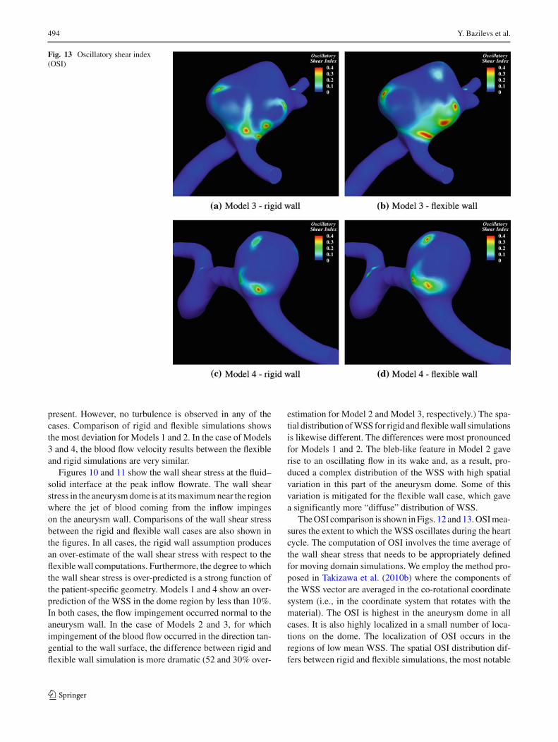
The OSI comparison is shown in Figs. 12 and 13. OSI mea-sures the extent to which the WSS oscillates during the heartcycle. The computation of OSI involves the time average ofthe wall shear stress that needs to be appropriately definedfor moving domain simulations. We employ the method pro-posed in Takizawa et al. (2010b) where the components ofthe WSS vector are averaged in the co-rotational coordinatesystem (i.e., in the coordinate system that rotates with thematerial). The OSI is highest in the aneurysm dome in allcases. It is also highly localized in a small number of loca-tions on the dome. The localization of OSI occurs in theregions of low mean WSS. The spatial OSI distribution dif-fers between rigid and flexible simulations, the most notable

123

Computational vascular fluid–structure interaction 495

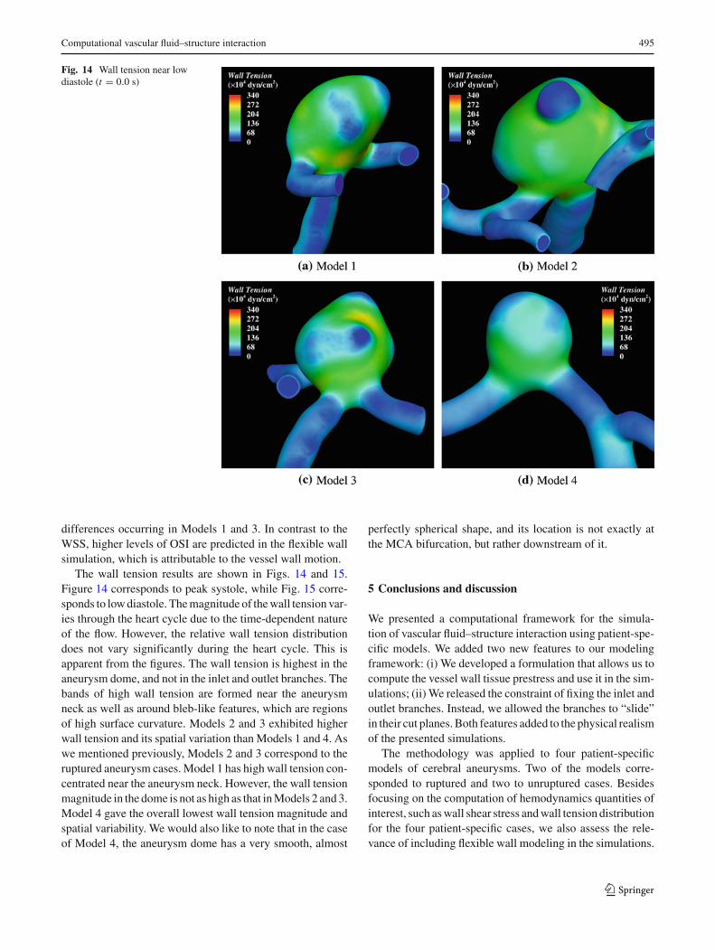
Fig. 14 Wall tension near lowdiastole (t = 0.0 s)

differences occurring in Models 1 and 3. In contrast to theWSS, higher levels of OSI are predicted in the flexible wallsimulation, which is attributable to the vessel wall motion.

The wall tension results are shown in Figs. 14 and 15.Figure 14 corresponds to peak systole, while Fig. 15 corre-sponds to low diastole. The magnitude of the wall tension var-ies through the heart cycle due to the time-dependent natureof the flow. However, the relative wall tension distributiondoes not vary significantly during the heart cycle. This isapparent from the figures. The wall tension is highest in theaneurysm dome, and not in the inlet and outlet branches. Thebands of high wall tension are formed near the aneurysmneck as well as around bleb-like features, which are regionsof high surface curvature. Models 2 and 3 exhibited higherwall tension and its spatial variation than Models 1 and 4. Aswe mentioned previously, Models 2 and 3 correspond to theruptured aneurysm cases. Model 1 has high wall tension con-centrated near the aneurysm neck. However, the wall tensionmagnitude in the dome is not as high as that in Models 2 and 3.Model 4 gave the overall lowest wall tension magnitude andspatial variability. We would also like to note that in the caseof Model 4, the aneurysm dome has a very smooth, almost

perfectly spherical shape, and its location is not exactly atthe MCA bifurcation, but rather downstream of it.

5 Conclusions and discussion

We presented a computational framework for the simula-tion of vascular fluid–structure interaction using patient-spe-cific models. We added two new features to our modelingframework: (i) We developed a formulation that allows us tocompute the vessel wall tissue prestress and use it in the sim-ulations; (ii) We released the constraint of fixing the inlet andoutlet branches. Instead, we allowed the branches to “slide”in their cut planes. Both features added to the physical realismof the presented simulations.

The methodology was applied to four patient-specificmodels of cerebral aneurysms. Two of the models corre-sponded to ruptured and two to unruptured cases. Besidesfocusing on the computation of hemodynamics quantities ofinterest, such as wall shear stress and wall tension distributionfor the four patient-specific cases, we also assess the rele-vance of including flexible wall modeling in the simulations.

123

496 Y. Bazilevs et al.

Fig. 15 Wall tension near peaksystole (t = 0.08 s)

The strain levels predicted in the simulations (reaching amaximum of 10–15% at peak systole) are sufficiently highto necessitate the use of large deformation theory for tissuemodeling. However, the strains are not sufficiently high to bein the regime of strong material non-linearity.

The results show that the interaction between the bloodflow and wall deformation significantly alters the hemody-namic forces acting on the arterial wall, with respect to rigidwall modeling. Rigid wall simulations consistently overes-timated the wall shear stress magnitude, on one case by asmuch as 52%, which, in our opinion is significant, given theimportance of this quantity of interest. In two of the cases,the gross features of the wall shear stress distribution on thearterial wall were significantly different for the rigid and flex-ible simulations. Rigid versus flexible wall simulation resultsreinforce the importance of using fluid–structure interactionin patient-specific modeling of cerebral aneurysms. Furtherobservations show that the magnitude of the wall shear stressis a strong function of the inlet branch orientation and theangle of impingement of the blood on the arterial wall.

Pathophysiologically, abnormal levels of WSS and OSIdegrade the vessel wall and initiate aneurysm formation, andbiomechanically, aneurysm rupture occurs when wall ten-

sion exceeds the wall tissue strength. The present simulationshows that WSS, OSI and wall tension are highly dependenton the three-dimensional conformation of the lesion. In theunruptured cases (Models 1 and 4), wall tension was rela-tively low and relatively evenly distributed in the aneurysmdome. In the ruptured cases (Models 2 and 3), wall tensionwas higher and distributed in a ring-formed shape aroundbleb-like formations on the dome. Model 1, the unrupturedcase, showed relatively high wall tension magnitude (and var-iation) compared to Model 4, but not to the extent of Models2 and 3.

A recent article Watton et al. (2009) identified anotherhemodynamic quantity that affects the growth and remod-eling of aneurysms, which is the wall shear stress gradient(WSSG). WSSG measures the spatial variation of the WSSin the vessel wall in-plane directions. In Watton et al. (2009),the in-plane gradient was easily obtainable due to the simplegeometry of the vessel employed. However, WSSG requiresan appropriate definition in the case of complex patient-spe-cific geometry.

The presences of localized blebs are known to be associ-ated with rupture. This might indicate that rupture occurredbecause of the strength of the wall tissue was exceeded by

123

Computational vascular fluid–structure interaction 497

the wall tension, leaving overstretched tissue remnants at therupture site. If reproduced in larger clinical series, this pro-posed computational method might be evolved to a tool forbetter prediction of future rupture risk. As a result, in thefuture, we plan to perform simulations of more patient-spe-cific models so as to enhance our understanding of the under-lying phenomena and their relationship to clinically observedevents.

The wall thickness is very hard or impossible to obtainexperimentally, so we plan to make use of the geometry data(such as local branch radii) and clinical experience of one ofthe co-authors to incorporate a reasonable wall thickness ofthe aneurysm dome and the surrounding branch vessels inthe simulations. Recent advances in high resolution MRI forcerebral aneurysms Ryu et al. (2009) leave us hopeful that inthe near future, blood vessel wall thickness may be obtainedthrough imaging, thus removing this uncertainty and burdenfrom the modeling.

We would like to note that the structure of arterial tissuegenerally changes abruptly in the neck region of an aneu-rysm from healthy tissue with an intact medial layer withinthe parent artery to thin collagenous tissue in the aneurysm.As a result, homogeneous isotropic material modeling thatis employed in this work may lead to inaccurate predictionsof the deformation field and thus inaccurate hemodynamicsolutions. A possible remedy for this will be to model healthyarterial tissue in the parent branches and collagenous tis-sue in the aneurysm dome. We hope to pursue this in futurestudies.

Another advantage of FSI over the rigid wall assumptionis that it enables the simulation of a complete mechanicalenvironment of the arterial wall, including the cells within,and, more importantly, its coupling to the hemodynamics. Forinstance, cyclic stretching may play a significant role withregards to functionality (e.g., gene expression or structuralalignment) of endothelial cells (Cummins et al. 2007),smooth muscles, and fibroblasts. This will, in turn, change theelastic properties of the arterial tissue and alter the responseof the coupled system.

Acknowledgments We wish to thank the Texas Advanced ComputingCenter (TACC) at the University of Texas at Austin for providing HPCresources that have contributed to the research results reported withinthis paper. This work was partially supported by a research grant fromthe regional health authorities in northern Norway. Support of TeragridGrant No. MCAD7S032 is also gratefully acknowledged. We thankProf. Tor Ingebrigtsen, Institute for Clinical Medicine, University ofTromsø, Norway, and the Department of Neurosurgery, the UniversityHospital of North Norway for generously devoting his time to discussand evaluate the results of this work and their relevance to clinicalpractice.

Open Access This article is distributed under the terms of the CreativeCommons Attribution Noncommercial License which permits anynoncommercial use, distribution, and reproduction in any medium,provided the original author(s) and source are credited.

References

Appanaboyina S, Mut F, Löhner R, Putman C, Cebral J (2009) Simula-tion of intracranial aneurysm stenting: techniques and challenges.Comput Methods Appl Mech Eng 198:3567–3582

Bazilevs Y, Calo VM, Zhang Y, Hughes TJR (2006) Isogeometric fluid-structure interaction analysis with applications to arterial bloodflow. Comput Mech 38:310–322

Bazilevs Y, Calo VM, Cottrel JA, Hughes TJR, Reali A, Scovazzi G(2007) Variational multiscale residual-based turbulence modelingfor large eddy simulation of incompressible flows. Comput Meth-ods Appl Mech Eng 197:173–201

Bazilevs Y, Calo VM, Hughes TJR, Zhang Y (2008) Isogeometric fluid-structure interaction: theory, algorithms, and computations. Com-put Mech 43:3–37

Bazilevs Y, Gohean JR, Hughes TJR, Moser RD, Zhang Y(2009a) Patient-specific isogeometric fluid-structure interactionanalysis of thoracic aortic blood flow due to implantation of theJarvik 2000 left ventricular assist device. Comput Methods ApplMech Eng 198:3534–3550

Bazilevs Y, Hsu M-C, Benson DJ, Sankaran S, Marsden AL(2009b) Computational fluid-structure interaction: methods andapplication to a total cavopulmonary connection. Comput Mech45:77–89

Brooks AN, Hughes TJR (1982) Streamline upwind/Petrov-Galerkinformulations for convection dominated flows with particularemphasis on the incompressible Navier-Stokes equations. Com-put Methods Appl Mech Eng 32:199–259

Castro MA, Putman CM, Cebral JR (2006) Computational fluiddynamics modeling of intracranial aneurysms: effects of parentartery segmentation on intra-aneurysmal hemodynamics. Am JNeuroradiol 27:1703–1709

Cebral JR, Castro MA, Appanaboyina S, Putman CM, Millan D,Frangi AF (2005) Efficient pipeline for image-based patient-spe-cific analysis of cerebral aneurysm hemodynamics: technique andsensitivity. IEEE Trans Med Imaging 24:457–467

Chung J, Hulbert GM (1993) A time integration algorithm for structuraldynamics with improved numerical dissipation: the generalized-αmethod. J Appl Mech 60:371–375

Cummins PM, von Offenberg Sweeney N, Killeen MT, Birney YA,Redmond EM, Cahill PA (2007) Cyclic strain-mediated matrixmetalloproteinase regulation within the vascular endothelium:a force to be reckoned with. Am J Physiol Heart Circ Physiol292:H28–H42

Fernández MA, Gerbeau J-F, Gloria A, Vidrascu M (2008) A parti-tioned Newton method for the interaction of a fluid and a 3D shellstructure. Technical Report RR-6623, INRIA

Figueroa CA, Vignon-Clementel IE, Jansen KE, Hughes TJR, TaylorCA (2006) A coupled momentum method for modeling blood flowin three-dimensional deformable arteries. Comput Methods ApplMech Eng 195:5685–5706

Figueroa CA, Baek S, Taylor CA, Humphrey JD (2009) A computa-tional framework for fluid-solid-growth modeling in cardiovascu-lar simulations. Comput Methods Appl Mech Eng 198:3583–3602

Formaggia L, Gerbeau JF, Nobile F, Quarteroni A (2001) On the cou-pling of 3D and 1D navier-stokes equations for flow problems incompliant vessels. Comput Methods Appl Mech Eng 191:561–582

Gerbeau J-F, Vidrascu M, Frey P (2005) Fluid-structure interaction inblood flows on geometries based on medical imaging. ComputStruct 83:155–165

Holzapfel GA (2000) Nonlinear solid mechanics, a continuum app-roach for engineering. Wiley, Chichester

Hughes TJR, Scovazzi G, Franca LP (2004) Multiscale and stabilizedmethods. In: Stein E, de Borst R, Hughes TJR (eds) Encyclopediaof computational mechanics, vol 3, Fluids, chapter 2. Wiley

123

498 Y. Bazilevs et al.

Hughes TJR, Cottrell JA, Bazilevs Y (2005) Isogeometric analysis:CAD finite elements, NURBS exact geometry, and mesh refine-ment. Comput Methods Appl Mech Eng 194:4135–4195

Humphrey JD (2002) Cardiovascular solid mechanics, cells, tissues,and organs. Springer, New York

Isaksen JG, Bazilevs Y, Kvamsdal T, Zhang Y, Kaspersen JH,Waterloo K, Romner B, Ingebrigtsen T (2008) Determination ofwall tension in cerebral artery aneurysms by numerical simulation.Stroke 39:3172–3178

Jansen KE, Whiting CH, Hulbert GM (1999) A generalized-α methodfor integrating the filtered navier-stokes equations with a stabi-lized finite element method. Comput Methods Appl Mech Eng190:305–319

Lagana K, Dubini G, Migliavacca F, Pietrabissa R, Pennati G,Veneziani A, Quarteroni A (2002) Multiscale modelling as a toolto prescribe realistic boundary conditions for the study of surgicalprocedures. Biorheology 39:359–364

Lipton S, Evans JA, Bazilevs Y, Elguedj T, Hughes TJR (2009) Robust-ness of isogeometric structural discretizations under severe meshdistortion. Comput Methods Appl Mech Eng 199:357–373

Marsden AL, Feinstein JA, Taylor CA (2008) A computational frame-work for derivative-free optimization of cardiovascular geome-tries. Comput Methods Appl Mech Eng 197:1890–1905

Nobile F (2001) Numerical approximation of fluid-structure interactionproblems with application to hemodynamics. Ph.D. thesis, EPFL

Rank E, Düster A, Nübel V, Preusch K, Bruhns OT (2005) Highorder finite elements for shells. Comput Methods Appl Mech Eng194:2494–2512

Rissland P, Alemu Y, Einav S, Ricotta J, Bluestein D (2009) Abdominalaortic aneurysm risk of rupture: patient-specific FSI simulationsusing anisotropic model. J Biomech Eng 131:031001

Ryu C-W, Jahng G-H, Kim E-J, Choi W-S, Yang D-M (2009) Highresolution wall and lumen MRI of the middle cerebral arteries at3 tesla. Cerebrovasc Dis 27:433–442

Scotti CM, Finol EA (2007) Compliant biomechanics of abdominalaortic aneurysms: a fluid-structure interaction study. ComputStruct 85:1097–1113

Sforza DM, Putman CM, Cebral JR (2009) Hemodynamics of cerebralaneurysms. Annu Rev Fluid Mech 41:91–107

Simo JC, Hughes TJR (1998) Computational inelasticity. Springer,New York

Takizawa K, Christopher J, Tezduyar TE, Sathe S (2010a) Space-timefinite element computation of arterial fluid-structure interactionswith patient-specific data. Commun Numer Methods Eng 26:101–116

Takizawa K, Moorman C, Wright S, Christopher J, Tezduyar TE(2010b) Wall shear stress calculations in space-time finite elementcomputation of arterial fluid-structure interactions. Comput Mech.Published online, doi:10.1007/s00466-009-0425-0

Taylor CA, Humphrey JD (2009) Open problems in computational vas-cular biomechanics: hemodynamics and arterial wall mechanics.Comput Methods Appl Mech Eng 198:3514–3523

Taylor CA, Hughes TJR, Zarins CK (1998) Finite element modelingof blood flow in arteries. Comput Methods Appl Mech Eng 158:155–196

Tezduyar TE (2003) Computation of moving boundaries and interfacesand stabilization parameters. Int J Numer Methods Fluids 43:555–575

Tezduyar TE, Sathe S, Cragin T, Nanna B, Conklin BS, Pausewang J,Schwaab M (2007) Modelling of fluid-structure interactions withthe space-time finite elements: arterial fluid mechanics. Int JNumer Methods Fluids 54:901–922

Tezduyar TE, Takizawa K, Moorman C, Wright S, Christopher J (2009)Multiscale sequentially-coupled arterial FSI technique. ComputMech. doi:10.1007/s00466-009-0423-2

Torii R, Oshima M, Kobayashi T, Takagi K, Tezduyar TE (2006a) Com-puter modeling of cardiovascular fluid-structure interactions withthe deforming-spatial-domain/stabilized space-time formulation.Comput Methods Appl Mech Eng 195:1885–1895

Torii R, Oshima M, Kobayashi T, Takagi K, Tezduyar TE (2006b)Fluid-structure interaction modeling of aneurysmal conditionswith high and normal blood pressures. Comput Mech 38:482–490

Torii R, Oshima M, Kobayashi T, Takagi K, Tezduyar TE (2007) Influ-ence of the wall elasticity in patient-specific hemodynamic simu-lations. Comput Fluids 36:160–168

Torii R, Oshima M, Kobayashi T, Takagi K, Tezduyar TE (2008) Fluid-structure interaction modeling of a patient-specific cerebral aneu-rysm: influence of structural modeling. Comput Mech 43:151–159

Torii R, Oshima M, Kobayashi T, Takagi K, Tezduyar TE (2009) Fluid-structure interaction modeling of blood flow and cerebralaneurysm: significance of artery and aneurysm shapes. ComputMethods Appl Mech Eng 198:3613–3621

Vignon-Clementel IE, Figueroa CA, Jansen KE, Taylor CA (2006) Out-flow boundary conditions for three-dimensional finite elementmodeling of blood flow and pressure in arteries. Comput Meth-ods Appl Mech Eng 195:3776–3796

Watton PN, Raberger NB, Holzapfel GA, Ventikos Y (2009) Couplingthe hemodynamic environment to the evolution of cerebral aneu-rysms: computational framework and numerical examples. J Bio-mech Eng 131:101003

Wolters BJBM, Rutten MCM, Schurink GWH, Kose U, de Hart J,van de Vosse FN (2005) A patient-specific computational modelof fluid-structure interaction in abdominal aortic aneurysms. MedEng Phys 27:871–883

Zhang Y, Wang W, Liang X, Bazilevs Y, Hsu M-C, Kvamsdal T,Brekken R, Isaksen JG (2009) High-fidelity tetrahedral mesh gen-eration from medical imaging data for fluid-structure interactionanalysis of cerebral aneurysms. Comput Model Eng Sci 42:131–150

Zunino P, D’Angelo C, Petrini L, Vergara C, Capelli C, Migliavacca F(2009) Numerical simulation of drug eluting coronary stents:mechanics, fluid dynamics and drug release. Comput MethodsAppl Mech Eng 198:3633–3644

123