Two mixed variational principles for exterior fluid-structure interaction problems

Compurers & Svumwes Vol. 33. No 3. pp. 621-635. 1989 Printed m Great Baitam.

0045.7949189 $3 cm + 0.00 G 1989 Per&awn Press plc

TWO MIXED VARIATIONAL PRINCIPLES FOR EXTERIOR FLUID-STRUCTURE INTERACTION PROBLEMS

PETER M. PINSKY and NAJIB N. ABB~UD

Department of Civil Engineering, Stanford University, Stanford, CA 94305. U.S.A.

(Received 15 August 1988)

Abstract-Two mixed variational principles for transient and harmonic analysis of non-conservative coupled exterior fluid-structure systems are proposed. The variational principles accommodate the dissipation associated with viscoelastic constitutive properties of the structure as well as the radiation boundary condition on the fluid. The principles are written for the physical system and its adjoint using the formalism introduced by Morse and Feshbach for dissipative systems. The mixed formulations use pressure and displacement potential scalar variables for the fluid and can incorporate a general class of local radiation boundary conditions. The finite element approximations based on these variational principles display a symmetric form for transient and harmonic problems.

I. INTRODUCHON

We consider in this paper the dynamic interaction problem of elastic-viscoelastic structures submerged in unbounded fluid domains. The exterior inviscid and irrotational fluid acts as an acoustic medium in which wave propagation phenomena result from either the scattering of incident traveling waves or the radiation of waves resulting from vibrations within the structure. The problem is approached within a variational framework amenable to computational treatment and we wish to consider variational principles for both the transient and harmonic analysis of the coupled system, where the latter is derived consistently from the former.

As examples of two-phase elastic-viscoelastic structures which are important in fluid-structure interaction, we note the increasing importance of elastic structures with compliant viscoelastic coatings. Applications include control of the radiation field surrounding a submerged structure, noise shielding in sonar arrays, and sound absorption in engines. The analysis and design of structures with compliant coatings are complex tasks which must include the characterization of the structural response as well as the surface deformations of the coatings. For example, Pinsky and Kim [ 1,2] have developed finite element models for multilayered elastic-viscoelastic coated shells including thickness deformation modes in the coatings.

Several issues need to be addressed in developing a formulation and a treatment scheme for this class of problems, one of which is the incorporation of dissipation into a variational principle. The dissipation associated with viscoelastic constitutive properties of the structure as well as the radiation condition on the fluid renders the coupled system non-conservative and thus impedes the use of the Hamilton variational principle. A modified formal-

ism, first introduced by Morse and Feshbach [3], will be used to develop variational principles governing the dissipative system.

A second issue is that the formulation must accommodate the radiation condition at infinity. Boundary integral techniques are particularly attractive in that they avoid the explicit imposition of the radiation condition by the use of the free space Green function or some series expansion representing the solution to the reduced wave equation in the exterior. Such techniques have been proposed for the Helmholtz equation in numerous works [4-IO]; codes have been developed for the coupled fluid-structure interaction problem by Everstine et al. [I l] and others. But the boundary integral formulations present several disadvantages:

(I) They usually lead to asymmetric coefficient matrices for the Helmholtz equation, thus requiring the adoption of either a non-symmetric system solver or of some symmetrization technique such as that proposed by Zienkiewicz ef al. [ 121.

(2) In spite of the reduction in the dimensionality of the problem, they remain computationally expensive in that the non-localization of the coupling over the boundary results in a full matrix that needs to be inverted. Expense is also incurred in the local increase in quadrature order [7], definition of singular elements [8], or other special treatments [4] required to resolve the singularity in the kernel of the integral equation.

(3) It is well known that the classical exterior integral equations for the Helmholtz equation admit non-unique solutions at resonant wavenumbers of a related interior problem. Numerical formulations based on these integral equations are singular at the critical wavenumbers and ill-conditioned near them. Although ‘improved’ formulations have been proposed to either mitigate this non-uniqueness problem

621

622 P. M. PINSKY and N. N. ABBOLJD

at low wavenumbers [5, IO] or to eliminate it com- pletely [6, 91, they invariably add to the complexity of the formulation and to the computational effort.

(4) Last but not least, the application of boundary integral techniques has been restricted until now to periodic fluid-structure interaction problems. Even

though Zienkiewicz et al. [13] suggested that the boundary integral approach could be extended to exterior transient problems, it would still be restricted

to linear problems for a solution via Fourier Transform to be feasible.

The classical boundary integral approach gives an integral representation to the entire fluid domain in

such a way that the ‘computational domain’ is effectively the physical boundary of the structure. An alternative method known as the coupled boundary and finite element method [l3, 141 divides the fluid

into an interior finite element region and an exterior domam with an integral representation, and couples the two over an artificial boundary. Though this method can incorporate inhomogeneities within the finite element acoustic region, it still suffers from the same deficiencies as the classical boundary integral

approach. A closely related method, the ‘Dirichlet-to- Neumann’ (DtN) method, has recently been pro-

posed [l5]. The DtN method seems promising for time harmonic analysis in that it overcomes some of the difficulties associated with the classical boundary integral approach. but it is not clear that it mitigates

the problem of interior resonances. But most impor- tantly, the DtN method for transient analysis leads to the formation of a convolution integral in time and the resultmg integro-differential system of equations, which is non-local in both time and space. would require modifications on standard integration

schemes as well as a substantial storage effort. Opposing the general class of non-local integral

approaches is the class of finite element methods with local boundary conditions. It includes methods such

as infimte elements, the Smith method, and various dampers. Infinite elements [l3, 16, 171 satisfy the radiation condition implicitly by their choice of shape functions, but once again they seem better suited for time harmonic problems. The Smith method [l8] solves the same problem twice. once with a Dirichlet boundary condition and another with a Neumann boundary condition. The superposition of the two solutions cancels all reflected waves, thus satisfying the radiation condition. This expensive method is highly accurate for transient analysis, but cannot be carried over to the time harmonic case.

In view of all the restrictions on the various methods reviewed above, and since we are interested in formulations applicable to both transient and harmonic problems, the damper concept is adopted here. The basic idea is for the damper to absorb outgoing waves entirely at an artificial boundary, thus inhibiting all reflections and simulating an infinite domain [19]. The damper in its simplest form, known as the plane wave damper, applies the

Sommerfeld radiation condition as a natural boundary condition on the fluid boundary. The per- formance of such a damper, though exact at infinity. deteriorates as the position of the artificial boundary approaches the source of perturbation, especially for longer wavelengths. In a recent extension to the damper concept, a family of differential boundary operators, based on a series solution of the wave equation, has been proposed for time dependent and harmonic problems [20. 311. As the order of the dtfferential operator mcreases, these dampers apply the radiation condition more and more accurately at a finite artificial boundary.

A third issue that needs to be addressed in

developing a finite element formulation for the fluid-structure interaction problem is that of the

choice of the fluid parametrizatton variables. The implications of various choices are reviewed m reasonable detail later in the paper. In the present

work, we advocate the USC of a mixed scalar--scalar formulatton as a means of combinmg the advantages of the popular [22] displacement-based vectorial

approach (symmetry) and pressure-based scalar approach (reduction in the number of unknowns and CI prrori satisfaction of the irrotationality condition).

We recall that the lack of symmetry has been held

against the collocation boundary integral method.

and now against the scalar-based fluid finite element formulation. These reservations are mottvated by the

fact that non-symmetry leads to greater requtrements for computer time and storage. and Inhibits the use of a large array of efficient algorithms and codes designed specifically to handle symmetric matrices. In addition, unsymmetric matrices associated with the discretization of self-adjoint operators, such as those arising from a collocation integral approach, are objectionable on theoretical grounds and can lead to

serious errors (e.g. imaginary eigenvalue components when none should exist). For the harmonic problem.

efforts have consistently been made to recapture the symmetry of both the system and its partitions, sometimes at considerable cost [ 12, 23 -261. For the transient problem, unsymmetric systems require special time-stepping algorithms for combined solution procedures [27], and they hamper the efficiency and stability of partitioned time-integrators to the extent that they may necessitate the use of special stabilization schemes [28]. In view of the above. mixed scalar formulations leadmg to symmetric coupled systems present themselves as a simpler, more direct, and computationally competitive

approach to the problem. In this paper we develop a vartattonal framework

for the transient and harmonic fimte element analysis of the coupled fluid-structure system depicted in Fig. 1. Using the Morse and Feshbach formalism for dissipattve systems, we start by formulating Lagrangians for the structure and the fluid separately. The structure Lagrangian can accommodate a general class of elastic-viscoelastic structures. Two differ-

Exterior fluid-structure interaction 623

n

Fig. I. Coupled system: domains and boundaries.

ent mixed fluid Lagrangians, employing pressure and displacement potential as variables, are derived variationally from a Hu-Washizu Lagrangian using Legendre transformations and the divergence theorem. The Class 1 and Class 2 fluid formulations diverge in their admissibility restrictions on trial functions and couple differently with the structure Lagrangian, though both result in symmetric and sparse systems of algebraic equations. The Lagrangian for the coupled problem is developed by adding the structure and fluid Lagrangians, and imposing compatibility constraints at the fluid- structure interface and the radiation condition at the artificial boundary. We use the plane wave damper, while recognizing its limitations, to demonstrate the methodology. We are presently working on extending the proposed principles to incorporate higher-order dampers.

The resulting coupled systems are easily specialized for the interior fluid-elastic structure interaction problem. For that, it suffices to eliminate those terms corresponding to the structural and radiation dissipation, We note that upon such a specialization in the frequency domain, the Class 1 and Class 2 systems reduce to Morand and Ohayon’s [29,30] ‘mass-coupling’ system and Ohayon’s [31] ‘stiffness- coupling’ system respectively. We also note that the specialization of the Class 1 formulation to the transient non-dissipative interior problem yields the system proposed by Geradin et al. [32].

In the first part of this paper we develop the structure Lagrangian. The second part of the paper develops the two fluid Lagrangians. The third part of the paper develops the coupled formulations and the paper concludes with a numerical example for the Class 1 formulation.

2. STRUCTURE

2.1. Background

As noted in the Introduction, we wish to consider structures which include viscoelastic material behavior. An example of such a structure is that of elastic shell structures with compliant coatings. Finite element formulations for such structures may be found, for example, in [l, 21. In this paper we do not consider specific structural models but wish to introduce a sufficiently general variational formulation to accommodate this class of problems. The approach adopted is to consider the structure to have general

viscoelastic constitutive equations which revert to linear elasticity for appropriate choices of the viscosity coefficients. In this way two-phase elastic- viscoelastic type structures may be modeled.

2.2. Viscoelastic constitutive equations

Three-dimensional constitutive equations for viscoelasticity can be constructed by combining three-dimensional generalizations of Maxwell and Kelvin elements. In the isotropic case, the decoupled deviatoric and dilatational responses are governed by differential equations of the general form [33]:

z (4k),z; (P~)~= 1 (2.14 k=O

kzo (PA s = k$o (& 1, F ; (PO), = 1, @lb)

where

S = u - (1/3)tr(u)l = deviatoric stress tensor

e = L - (1/3)tr(c)l = deviatoric strain tensor

a, = (1/3)tr(a) = hydrostatic pressure

cr = tr(e).

The subscripts d and c identify parameters related to the viscoelastic model governing the deviatoric and dilatational responses respectively.

In developing the formulation of the transient analysis of the coupled problem, we shall restrict ourselves to a constitutive equation based on a single generalized Kelvin element (md = m, = 0; n,, = n,. = 1). In this case:

a=J,:e+J?:L’ (2.2a)

J,= f(3K -3/i)1 @ 1+2/ii-i (2.2b)

52 = f(39 - 2r7)l @ I + 2rl~ (2.2c)

where 1 is the second-order unit tensor, ll is the fourth-order unit tensor, 1 and K are the Kelvin element shear and bulk moduli respectively, q and 9 are the Kelvin element deviatoric and dilatational viscosity coefficients. This restricted model obviates the need for integration algorithms associated with rate constitutive equations, by giving rise, explicitly, to consistently derived constant stiffness and damping matrices, K, and K, respectively.

The viscoelastic model used for the fiequency- domain analysis is based on a generalized Kelvin chain with an arbitrary number of elements (Fig. 2). In this case, equations (2.1) are recast in the form:

a0 e’“” = [J,(w) + iwJ,(w)]: co e”“’

= [;(3K(w) - 2G(w))l@ 1 + 2G(w)I-I]:

co et”“, (2.3a)

624 P. M. PINSKY and N. N ABBOUD

‘71 J 19r

Frg. t. Vrscoelastic model

where K(o), G(o)EC and u09 &,~a=’ and J,(W), J*(W) e R4, and

G(m)=X(@ +;LqJ+$

(2.3b)

I i ,

(2.3~)

The constitutive relation (2.3) produces a frequency dependent contribution to both the stiffness and damping terms, K, and Kz respectively. J, and J,, and consequently K, and KZ, will be in general functions of both elastic and viscous material parameters.

Remarks

(I) The above constitutive modeling of the viscoelastic coating is novel in that it is derrved from a ‘continuum’ model whose parameters can be determined in the laboratory.

(2) The viscoelastic model reverts to linear elasticity in the fimiting case of null viscosity coefficients.

(3) The viscoelastic model parameters may be made dependent on the hydrostatic pressure 0, by use of internal variable theory. Such an extension is planned for future study of the effects of increasing hydrostatic pressure on the behavior of the dissipative coatings.

2.3. Structure Lagranglan

It is well known that the introduction of dissipative terms impedes the use of the Hamilton variational formalism for conservative systems. To overcome this difficulty, a modified formalism for dissipative systems was first introduced by Morse and Feshbach [3], and has been used by Gladwell [34] and Graggs 135,361 for damped acousto-structural problems. The procedure involves the use of a ‘mirror-image’ adjoint system in which energy accrues as it is being dissi- pated in the physical system. The extended system is thus conservative and the equations of motion can be written in Hamilton’s canonical form. The first variation of the resulting functional with respect to the adjoint variables (denoted by an asterisk in this paper) gives rise to the Euler-Lagrange equations

governing the physical problem, while the variation with respect to the original variables yields those governing the adjomt problem. The above variational approach is employed here to form the functional describing the motion of the shell~oatings-fluid coupled system.

The structure Lagrangtan YJ = $ - ‘f i, in which T is the kinetic energy and ‘I ;is the potential energy, has the form:

f2.4a)

s (Vu,:J,:Vu,*+Vu,:J,:Vu,*)dR a.

+4’ s (Vu,* : J1 : Vi, + Vu: : Jz : V1, 0,

- Vu, : J2 : Vu,* - Vu, : J: : Vu:) dR

1 --j-

1 (i;u,*+i;u,*+p u,.+~;.u,)dl-,

i, (24b)

where u = u,+ iu, is the structure complex displacement vector, t = t, + ii, is the external complex traction vector applied on r,, and p, is the structure density.

The Lagrangian Su, describes the motion of a generic structure in t’acuo. Later, a loading term representing the interface interaction on r, will arise naturally from the coupling procedure. We note that the energy terms in 9, are real. even though the field variables are assumed to be complex to allow for the harmonic time de~ndence case. We further note that the energy terms’ coefficients are chosen such that the variables revert to root mean square (r.m.s.f quantities. which remam constant in time, in the harmonic case.

3. FLUIll

3.1. Background

Several formulations for the analysis of fluid-structure interaction problems have been proposed. Whereas they invariably agree on the choice of the dispia~ement as the structure’s variable,


they differ in the fluid representation which we use to distinguish four categories of formulations.

(I) Vectorial formulations j22, 37,381: A tensorial field, typically the displa~ment, is chosen to represent the fluid response. The ease of incorporation into standard displacement-based finite element codes and the symmetry of the resulting coupled system of equations render such formulations popular, but they do exhibit some major disadvantages such as the excessive stiffness of the elements, thus requi~ng reduced integration, the need to introduce a penalty constraint to inhibit spurious rotational modes, and the desirability of decoupling the tangential displacement degrees of freedom at the fluid-structure interface.

(2) Scalar fo~ulations 122, 341: A scalar field such as the pressure, the displacement potential, or the velocity potential is used as the unknown fluid variable. The reduction in the number of fluid degrees of freedom and the apriori satisfaction of the irrotationality condition constitute the main advantages of scalar formulations over the vectorial ones. However, single-field scalar fo~ulations give rise to an unsym- metrical system of equations for the coupled problem, thus requiring special handling and inhibiting the use of the standard algorithms for symmetrical systems.

(3) Mixed scalar-vectorial formulations: The fluid is represented by both scalar and vectorial variables. Such an approach has been used by Liu and Chang 1391, Taylor and Zienkiewicz 1401, and Fenves and Vergas-Lob [41].

(4) Mixed scalar-scalar formulations: Two scalar fields, which are approximated independently, are chosen to represent the fluid. Morand and Ohayon 129, 301 introdu~d first a ‘mass-coupling’ pressuredisplacement potential formulation for the eigenvalue analysis of the interior fluid-structure interaction problem; Ohayon [31] later suggested a ‘stiffness-coupling’ counterpart. Geradin et al. [32] extended the ‘mass-coupling’ formulation to the transient analysis of the interior problem. Olson and Bathe [42] proposed a pressurevelocity potential formulation for both the transient and the eigenvalue analysis of the interior problem, and have shown its superiority over the fluid displacement formulation as the state of incompressibility is approached. In this paper we propose a mixed scalar-scalar fo~ulation for the exterior fluid-structure interaction. The salient features of the mixed scalar-scalar approach are the reduction in the number of unknowns when compared to a fully or partially vectorial approach, the u priori satisfaction of the irrotationality condition, and the resulting symmetry of the coupled system of equations as opposed to a single scalar field formulation.

In the following sections, we develop both the Class 1 (‘mass-coupling’) and the Class 2 (‘stiffness- coupling’) pressure-displacement potential formulations for the transient and harmonic analysis of the exterior interaction problem.

3.2. Governing equations for the @id

The classical acoustic approximation for Small amplitude motions of an inviscid and irrotational barotropic fluid admits as governing equations:

the momentum balance equation:

p+pOd;=O in&P&

the continuity equation:

(3.1)

p + ,00V2$ = 0 in Sz, (3.2)

and the equation of state:

p - c2p = 0 in Q,, (3.3)

where 4, p, and p are small perturbations in the displacement potential, pressure, and fluid density from the reference state of zero displacement potential, hydrostatic pressure p0 % p. and constant density p0 9 p. c is the velocity of wave propagation, which is assumed constant. It is worthwhile noting that the inclusion of cavitation effects would require c to be density dependent [“rl].

For reasons which will become apparent, we note that eliminating the variable p recasts the Auid field equations in the form:

p -I- p,J = 0 in rZ, (3.4)

p -t-p0c?V2~ =O in Q, (3.5)

whereas the elimination of both p and p, or p and (b yields the classical wave equation in the remaining variable:

V2p -(l/c2)p =O inn, (3.6)

V%#J -(l/c’)$ = 0 in Cl,. (3.7)

Conditions prevailing at the fluid boundary rl = r, u r, will be discussed in Sec. 4.

3.3. Three -$efd fluid Lagrangian

The Hu-Washizu Lagrangian for an elastic medium is given by

An acoustic fluid can be viewed as an elastic medium with a purely volumetric response and thus, the three-field fluid Lagrangian is given by

626 P. M. PINSKY and N N. ABBOLD

Although the subsequent development will only keep Using the divergence theorem on Y,in (3. lob) gives

p and # as the fluid variables, its generalization to Y,* = $ - Y ;?. where

include p as a variable is straightforward.

3.4. TW $eld fluid Lugrangtan (3.13a)

Enforcement of the equation of state (3.3) in (3.9) yields -sP, = + Y;, where the kinetic energy 4 and the potential energy I’; are given by

Y,?= -&j/dQ+ jn)VpV#dQ

P

Using the divergence theorem on different parts of 9,

- pV$ v dl-. (3.13b) 3;=;p” s Vd;.Vtt;dQ (3.lOa) ? Y;= - i jo,p’dR - jn,/++ dR. (3.10b)

Resorting again to the Morse and Feshbach formalism, we rewrite the Class 2 fluid Lagrangian as

gives rise to two possible fluid Lagrangians.

3.5. Class I formulation

Performing a Legendre transformation on q in (3,lOa) and using the divergence theorem gives:

I -- (VP, v4: + VP,. Vd,* J 2 Ri

+ VP:. V4, + VP,?. V#,) dR

- po s

cjW$ dQ + pi, % s

(bV4 . v dr, + p.374,). 11 dr (3.14) rl

where v is the unit outward normal vector to the fluid domain. Using the continuity eqn (3.5) to eliminate 4. COUPLED PROBLEM V%$ in 9; and Vz~ in &T,. we obtain $P,, = .q, - Y ;, , where The Lagrangian for the coupled problem is ob-

tained by adding the Lagrangians for the solid and

(3.1 lb)

the fluid domains. and imposing the appropriate constraints at the structure-fluid mterface r, and at the truncation boundary f , .

The fluid and structure are coupled by a kinemattc boundary condition that provides for the compatibility of the normal displacement at the interface and by a dynamic boundary condition that enforces the equilibrium of the hydrodynamic forces on f,:

Anticipating the introduction of dissipative effects, we use the Morse and Feshbach formalism for non- conservative systems to rewrite the Class 1 fluid Lagrangian as

u.n=V# .n

(r. n = -pn = p(,d;n.

The constraint at r, will ensure the satisfaction of the Sommerfeld radiation condition:


where

n = -v on r, = unit outward normal to the structure boundary r, u To.

n=v on r,- -unit outward normal to the fluid radiation boundary I-,.

The application of the radiation condition to the total fields p and 4 limits the formulations here developed to radiation problems. The proposed principles can be easily extended to scattering problems. This is done by applying the radiation condition to the scattered components of p and b, rather than to the total fields.

In Sets 4.1-4.3 we consider the Class 1 time domain formulation, its finite element discretization, and the corresponding frequency domain formulation. The Class 2 counterparts are presented in sets 4.44.6.

4. I. Ciass 1 time domain ~orrn~latio~

The Class 1 Lagrangian for the total system is

Y,=Y,+Y,,

+ ; s [A,(li,* - V#t,*) + A,(u,* - V#,‘) I-,

+ i,*(ti,-- Vq$)+ A,*@,-- V&J. nd!-

where I,, I., , jL y*, A,*, y,, y, , y ,* and y ,* are Lagrange muItipliers.

The stationarity of:

subject to

6p, = 6p, = sp,+ = sp,* = 0

sq5,=sf#J,=s~:=&#3,‘=0

i

at t = to and t = t,

~#~=~#~=~~~=~#~=o

identifies the Lagrange multipliers as:

1, = YI = -Pok I, = Y, = --P,d,

A,* = r,* =: -pO&; n: = r) = -p&,

and yields the following Euler-Lagrange equations:

V. o - p,; = 0; V. u* - p,,ii* = 0 in f& (4.2)

a.n--i=0; a*.n--i*=O onr, (4.3)

o.n-pOd;n=O; a*.a-p,qb'*n=O onr, (4.4)

G.n-VfJ.n=O; b*.n-ViJ*.n=Oonr, (4.5)

p+po$=o; p*+pofj*=O inn, (4.6)

i;+p0c2V2$=O; i;*+p,c2V2rj;*=Oinf$ (4.7)

Vd;.n+~$=O; V$* .n--iq*=O onr,.(4.8)

Remark I. The above Class 1 formulation requires the finite element approximations on u, p, and d, to be u E CO@,), (h E CO@,), and p E L,@).

Remark 2. Alternative constraint at rX. Consider the ‘mixed’ version of the Sommerfeld

radiation condition obtained as follows:

(radiation condition on 4)

p + PO+ = 0 in Q, (momentum balance)

I =+Vdj.n--p =0 on rx

POC (‘mixed’ radiation condition).

Had we used instead of the last integral in (4.1), the following Lagrange constraints:

we would have obtained as Euler-Lagrange eqns (4.2) to (4.7) and instead of (4.8):

V$.n-h$ =O;

(4.9)

(b =o; (6=00nr,, (4.10)

where it should be noted that condition (4.10), even though valid at infinity for problems exhibiting a decaying solution, tends to be too strong at a truncation boundary located at a finite distance. The results of a numerical application seem to substan- tiate the fact that such an alternative formulation is inappropriate.

628 P. M. PINSKY and N. N. ABBOUD

4.2. Discretization qf the Class

We adopt independent finite

tions for the system variables:

I Lagrangian

element approxima-

u(x, t) = (N,(x))d(t) E C"(Q,)

~6. t) = (N,W)p(t) E L,(R,)

4(x, t) = (N&M(t) E Co@,).

The discretization 62, = 0 gives rise to the following matrices:

“,I

K,=K:=A 1

(VN,,)rj,(VN,,) dR’ ?=I n:

-structure stiffness (4.11)

%/

Kz=K’=A s

(VN,,)%(VN,) dn’ <=, n:

-structure damping (4.12)

HI / M=M~=A p,N!N,,dn’

s I,=, n:

--structure mass (4.13)

11, I

Q=Q'=A s 1 N;N, dn’ <=I n;Po’.?

-flutd stiffness (4.14)

11, / E=E’=A

s P,,W,)~(VN,J dR”

c=l 0; -fluid mass (4. IS)

% / g=KT=A

s 5 N;N, dT”

(,=I I’, (’

-radiation damping (4.16)

? f=r;l N,ridI-’

s e=l 1:

--force vector (4.17)

)I< / c, =A

s - p,,N;nN, df’

<=I , Id’

-coupling matrix (4.18)

where

-coupling matrrx (4.19)

A = assembly operator L’= I

3, and j2 = matrix counterpart of tensors J, and J2, and the resulting svstem of eauations. corresuonding

to the stationarity of #, with respect to the adjomt

It is worth noting the followmg:

(4.20)

(I) The system (4.20) presents a symmetric and very sparse structure.

(2) The coupling of fields occurs m the extended mass matrix. The Class 1 formulation 1s thus of the

‘mass-coupling’ type. (3) The elimination of dissipative terms (i.e.

K, = B = 0) yields the system proposed by Geradin et (11. [32] for the transient response of an elastic enclosure filled with a compressible fluid.

(4) The variables in (4.20) have been assumed complex to make allowance for the case of harmonic

motions with dissipative effects. In transient analysis, however, the field variables need only be real.

As already noted. p needs only be integrable over R, and accordingly we consider a finite element approximation which is discontinuous across inter- element boundaries. A static condensation, at the

element level, of the pressure parameters is thus possible.

The weak form of the momentum balance equation

corresponding to the stattonarity of ,$, with respect

to p: and p: yields

p’= -(Q’)~‘(D;)# (4.21)

and the matrtx system (4.20) reduces to

_D& ,D,]{:]={;]’ (4.22)

where (D:)(Q))‘(D,) is actually formed as

@T)(Q) 'CD,)= A~YK~ ‘UK). (4.23) I,_,

The resulting system, although symmetric, involves five time orders. To reduce the number of time orders,


we set:

$ = 6 =I fluid acceleration potential

and the reduced system is rewritten, with an obvious loss of symmetry, as

Invoking the limitation principle for mixed finite elements [43,44], it should be noted that choosing N; = N; is equivalent to a pointwise enforcement of the momentum balance equation (3.1). In that case:

,=+

and the reduced system (4.24) degenerates to one corresponding to the discretization of a functional with a single-field @) fluid Lagrangian [22]. Thus, to retain the advantage of a mixed formulation, the order of spatial approximation of #J should be kept

higher than that of p. The improved p~ction of the displacement potential # is balanced by a deterioration of the pressure solution as obtained from (4.21). This deterioration is avoided by solving for p through a direct application of the momentum balance equation (3.1) during the post-processing phase of the finite element solution.

4.3. Class I frequency domain formulation

The Lagrangian 9, in (4.1) governs a system driven by an arbitrary time-dependent forcing function. If that forcing function can be expressed as a periodic function (or as a series of periodic functions via Fourier transforms), then the response of a linear system will have the same periodic form and the time dependence can be eliminated from the problem,

tie therefore consider the case:

u(x, 1) = U(x) e”‘; u*(x, t) = U*(x) eRuz

p(x, 1) = P(x) e”‘; pqx, 1) = P*(x) e””

4(x, 1) = e(x) e”‘; Ql(x, t) = a+(x) ebf

i(x, t) = T(x) em’; 7*(x, t) = T+(x) L’

f(t) = Fe”‘; P(t) = F* em’.

The variational problem becomes

where

1 -a2 -- I s 2 Qf ~,,(U,u,z + UjUi+) dI-2 + f

J‘ p&D,U,* + @,UT -I- @TV, + @,W,) . ill df

r,

f (P,@: + Pi@? + P,*@, + P:@J dQ

n/

(4.25)

As noted in Sec. 2.2, J, and Jr are functions of both elastic and viscous material properties, and the frequency w. The corresponding complex system of equations takes the form:

--2[~ $ CA3 33/3--B

630 P. M. PINSKY and N. N. ABEKWD

or equivalently written as a real system of equations:

-K, 0 0000

0 K, 0 0 0 0

0 OQOOO

0 0 OQOO +OJ 0 0 0 000

0 0 0000

-d

0 -K2 0 0 0 0 1 K, 0 0 0 0 0

0 0 00 0 0

0 0 00 0 0

0 0 00 0 -w’B

0 0 0 0 w2B 0

M 0 0 0 C, O 11 0 M 0 0 0 C,

0 0 0 0 D, 0

0 0 0 0 0 D,

Cf- 0 D; 0 -E 0 0 Cf 0 DT 0 -E -I D, D, p, P, @P, 9,

=

F, F, 0

0

0

0

(4.27)

We note the following: (1) Elimination of the extended damping matrix

reduces (4.26) to the real ‘mass-coupling’ system in [29,30] for the eigenvalue analysis of an elastic tank filled with a compressible fluid.

(2) The extended stiffness and mass matrices in (4.27) exhibit a symmetric structure, while the extended damping matrix exhibits a skew-symmetric one. The system (4.27) can be symmetrized by replacing the imaginary variables in the solution vector by their negatives and multiplying the corresponding columns in the coefficient matrices by - 1.

subject to

identifies the Lagrange multipliers as

2, = ;‘, = -p, : i, = I’, = -p

4.4. Class 2 time domain fbrmulatlon i* = y,* = -p,*; I j.: zz jl: = -p:,

The Class 2 Lagrangian for the total system is yielding the following Euler-Lagrange equations:

1pz = =!Y, + Y,l v u - &ii = 0;

+; s

~, [I,(uf - V4,*) + i,(u,* - Vl#J,*) V . u * - p,ii* = 0 in Q, (4.29)

+ i,*(u, - V@,) + i,*(u, - V$,)l n dT a.n-i=O;

a*.n--i*=O on r 0 (4.30)

u.n+pn=O;

a*.n+p*n=O on r, (4.31)

+ y:(v$;n+~q’i)]df n.n-Vb.n=O;

n*.n-V4*.n=O on r, (4.32)

s r,$L~~~:+m’,i:-L:i,-i:iJdr (4.28)

where i 1 i* i* I? ,, -, . , , yr, 7,. y,* and A,* are Lagrange

multipliers. The stationarity of

(Vp + p,V$) n = 0;

(VP* + pOV$*). n = 0 on r, (4.33)

v (Vp + poV$) = 0;

V.(Vp*+poV$*)=O in R, (4.34)

A = s

” Z1 dt p + pOc’V~@ = 0;

10 p*+p0czV2d*=0 in R, (4.35)


V$ ..+$3 =o;

vtp*.“+;fj*=O on rs (4.36)

(VP .n+f~)+po(vdi ..+f$)=o;

( Vp’.+* > ( +po vm.*.+* > =()

on Tm. (4.37)

Remark 1. The above Class 2 formulation requires the finite element approximations on II, p, and 4 to be u E CO(n,), 9 E Co&I,), and p E Co@,).

Remark 2. Alternative constraint at Tm. Had the last integral in (4.28) been omitted, we

would have obtained the Euler-Lagrange equations (4.29) to (4.36) but (4.37) would have appeared as:

(VP .“+~,)+p,vm...=o:

( VP* .“+*

) +p,Vd;*.n=O on rm.

Once more, this condition, though true at infinity for problems exhibiting a decaying solution, is erroneous at a truncation boundary located at a finite distance.

4.5. Discretization of the Class 2 Lagrangian

We adopt different finite element approximations for the system variables:

u(x, t) = (N,(x))d(t) E CO(n,)

P(X, 1) = (N,(x))p(t) e Co($)

4(x, t) = (N,(x))$(t) l CO($).

The discretization of SjZ = 0 gives rise to the following matrices:

C2 = ;i: s e-1 r:

NFnN, dP


Dz = ;i: s e-1 fI;

(VNJr(VN,) d.@


A=;i s 1 N,@#J dr’ e-l r’,c

-radiation damping. (4.40)

K,, Kr, M, Q, E, B, and f are as defined previously in (4.1 l)-(4.17); and the resulting system of equations takes the form:

The above system exhibits again a symmetric and sparse structure, and is of a ‘stiffness-coupling’ type. It also shows an improved bandedness when compared with the system (4.20) emanating from the Class 1 formulation. The radiation damping mani- fests itself in the Class 2 formulation through the two matrices A and B, in contrast to the Class 1 formulation which gives rise to a B matrix only.

4.6. Class 2 frequency domain formulation

As for Y,, we consider for 5?r the case

u(x, t) = U(x) era’; u*(x, t) = U*(x) el”’

p(x, t) = P(x) erwr; p*(x, t) = P*(x) em’

4(x, t) = a(x) e”‘; 4 *(x, t) = Q*(x) e’o’

1(x, t) = T(x) em’; 1*(x, t) = T*(x) eau’

f(t) = F e’““; P(t) = F* ewr.

The variational problem becomes:

6 P&u) = 0

where

s (V;T:+U;T~+Uf.T,+u~.T,)dr

r.

-k (p,U,z+P,U:+P,+U,+P,+U,).ndr s r,


-;

s (VP/V@:+VP,V@~+VP~VQ,+VP~V@,)d~+& n

s (P,P: + P, P:, dR

nf 0 I

(VU,:J,:VU;-VU,:J,:VU:)dR-& s

(P,@:+@,P: - P,+ap, - @:P,)dT r,

p,(U,U,* + U,U:) dn - f po(V@, . V@: + V@, . VO,*) dQ

Po(@,@:-@F@,)dP

and the corresponding complex system of equations takes the form

{[ii ;; j-if jT _;;.]-d[?f % H]}{;}={;} or equivalently written as a real system of equations:

K, 0 C2 0 0 0

0 K, 0 C> 0 0

Cf 0 -Q 0 Dz 0

0 cp 0 -Q 0 D2

0 0 D; 0 0 0

0 0 0 D; 0 0

+W

-CO2

0 -K? 0 0 0 0

K> 0 0 0 0 0

0 0 0 0 0 -A

0 0 0 0 A 0

0 0 0 -A’ 0 02B

0 0 AT 0 -w’B 0

MOO000

OMOOOO

0 00000

0 00000

0 OOOEO

0 OOOOE

F, F, 0

0

0

0

(4.42)

(4.43)

We note the following: (1) Elimination of the damping terms from Y2(w)

gives rise to the ‘stiffness-coupling’ formulation proposed by Ohayon [31] for the eigenvalue analysis of an elastic tank filled with a compressible fluid.

(2) Again, the extended stiffness and mass matrices in (4.44) are symmetric, whereas the extended damping matrix is skew-symmetric. The system (4.44) is symmetrized by replacing the imaginary variables in the solution vector by their negatives and invert- ing the signs of the corresponding columns in the coefficient matrices.

5. NUMERICAL EXAMPLE

We consider the problem of a submerged sphere of inner radius b, outer radius a, and density pS, whose inner surface is pulsating uniformly with a periodic radial displacement ti = oe’““. The dilatational response of the sphere is based on a viscoelastic constitutive equation of the form

0, = [j,(w) + iwj2(w)lc;

where (I~ and t, are the stress and strain radial components.

Because of the spherical symmetry, it suffices to discretize a single solid sector subtending angles of 1 rad at the center and, thus, the problem is essen- tially one-dimensional. The structural part of that sector is idealized as a single-degree-of-freedom oscillator with consistently derived stiffness, damping, and mass matrices based on a linear finite element approximation.

5. I. Exact solution

An exact solution to the idealized coupled problem can be derived. The boundary value problem is formulated as:

VP + k?P = (d2P/dr2) + (2/r)(dP/dr) + k2P = 0

for r e]a, +c0[ (5.1)

dP/dr = poo’U at r = a (5.2)

hU+t?u+a2P=0 at r =a, (5.3)

where


The solution of @.I)-(5.3) yields the expression for the pressure in the fluid as

k = w/c = wavenumber

U = complex displacement on r,

h = (j, + iwj,)(a2 + ab + b2)/31

- 02p,(6a2 + 3ub + b2)1/30

h= -(ji+hj2)(a2+ab +b2)/31

- 02p,(3a2 + 4ub + 3b2)1/60

P(r) = poo2u2 KU 1

h(1 + iku) - P&IA? T x e-tk(r-o)

5.2. Application

(5.4)

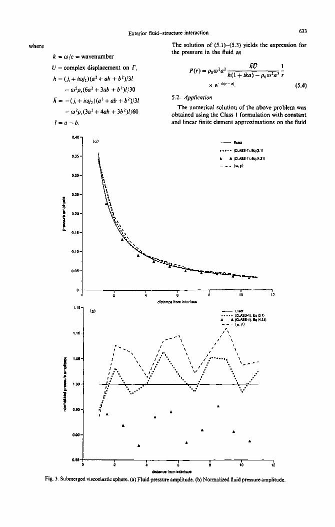
The numerical solution of the above problem was obtained using the Class 1 formulation with constant and linear finite element approximations on the fluid I=u-b.

0.40

0.35

0.20

0.25

4

1 0.20

$

B 0.15

0.10

0.05

- Exlcl

. . . . . oxAs6-1).Eq(3.0

. A (CUSS-l).Eq.t421)

-__ (U.P)

0 , I I I I I 1 0 2 4 6 8 10 12

distance from interface

tb) - Exacl . . . . . (CLA55-1).Eq(31) . A tcussll,Eqt43o --- (WP) ,

I\

*@’ / \ IC \ / \

*. I \ I \

I -. I \ / \

I \ \ /

\

I \ , .*.

\ I : l . \

I I .

. . . . ...* \

I .

\ ‘: l . \ l . \ ,” ‘. __-- \

I 5 ‘. I : l

\

‘. I : .*

,,$:* l . \/ l

l . l ’ . . .

. :

: 0. . l .

1: . . . . .**

1.’ ‘. .** . - .

c ‘.“. l . :*

‘..’ .

c

. . A

. . .

I I I I I I 2 4 6 2 10 12

Fig. 3. Submerged viscoelastic sphere. (a) Fluid pressure amplitude. (b) Normalized fluid pressure amplitude.


pressure and displacement potential respectively. A fluid domain of length 10 times the radius a of the sphere was discretized by 10 elements. The densities and elastic moduli of the structure and the fluid were chosen in ratios typical of steel-water systems. The values used were

2.

3.

4

excitation: w = 1 and D = (0.5) + i(0)

fluid: PO= 1 and c=l

sphere: PI = 8~0 and j, = lOOp,c* = 100;

a = 2b = 1 and jZ = 0.3j, = 30.

The Class I fluid pressure solution 1s compared in

5.

6.

7.

Fig. 3 with both the exact solution and the one obtained from the single-field pressure formulation (u, p). Both the single-field and the Class 1 mixed formulations capture the solution well. The (u, p) formulation produced an L, norm of the pressure amplitude error of 6.67%. In contrast, the proposed Class I pressure amplitude solution [as obtained from the displacement potential solution via (3.1)] reduced the Lz norm of the error to 4.17%. The Class I pressure amplitude solution as obtained from (4.21) exhibits an Lz norm error of 7.60%.

8

9

10

II

6. CONCLUSIONS 12.

Two new mlxed variational prmciples have been developed for the exterior fluid-structure interaction problem, for both transient and periodic solutions. In particular, the variational formulation accom- modates dissipation associated with the viscoelastic material properties of the structure as well as the radiation boundary condition on the fluid. The mixed formulations use scalar-scalar variables for the fluid. The salient features of the proposed mixed formulations are the reduction in the number of unknowns when compared with a fully or partially vectorial approach, the a priori satisfaction of the irrotationality condition, and the resulting symmetry of the coupled system of equations as opposed to a single scalar field formulation. Numerical results obtained from the Class 1 variational formulation in the frequency domain appear to be satisfactorily accurate. Further study of the numerical aspects of these formulations seems warranted. The extension of the proposed principles to incorporate higher- order dampers for the enforcement of the radiation condition is presently being investigated.

13.

14.

IS.

16.

17. 0. C Zienkiewicz and P. Bettess, Infimte elements m the study of fluid-structure Interaction problems. Lecture Notes In Physics, No 58. pp. 133-172 Springer, Heidelberg (I 976).

18. W D. Smith. A non-reflecting plane boundary for wave propagation problems J Compur Phys. 15. 493-503 (1974)

Acknowledgemenr-The material in this paper is based upon work supported by the Office of Naval Research under Grant No. N00014-84-K-0715. for which the authors are grateful.

19. 0. C. Zienklewlcz. D. W. Kelly and P. Betess, The Sommerfeld (radiation) condition on mfimte domains and its modelling in numerical procedures. Comput. Meth. appl. Sci. Engng, 3rd Int. Symp. IRIA Laboria (1977).

REFERENCES

20. A. Bavliss and E. Turkel, Radlatlon boundary con- ditlons for wave-like equations Commun. Pure appl. Math. XXXIII. 707-725 (1980).

1. P. M. Pinsky and K. 0. Kim, A multi-director formulation for elastic-viscoelastic layered shells. Inf. J. Numer. Meth. Engng 23(12), 2213-2244 (1986).

21. A. Bayliss. M: Gunzberger and E. Turkel. Boundary conditions for the numerlcal solution of elliptic equations in exterior regions. ICASE Rep. 8&l, NASA. Langley (1978).

P. M. Pinsky and K. 0. Kim, A multl-dlrector formulation for nonlinear elastic-viscoelastic layered shells Comput. Struct. 24(6), 901-913 (1986). P. M. Morse and H. Feshbach. Methods of Theoretrcul Physics. McGraw-Hill, New York (1953). G. Chertock, Integral equation methods on sound radiation and scattering from arbitrary surface David W Taylor Naval Ship Research and Development Center, Report 3938 (1971). H. Schneck, Improved Integral formulation for acoustic radiation problems. .I .4rousr Sot Am. 44, 41 58 (1968) A. J Burton and G I- Miller. The application of Integral equation methods to the numerical solution of some exterior boundary-value problems. Proc. R. SW. Land. A323, 201-210 (1971). D. T. Wilton, Acoustic radiation and scattermg from elastic structures. Int. J Numer Mefh. Engng 13, 123-138 (1978). I C. Mathews. NumerIcal techmques for three- dlmensional steady-state flu&structure interactlon. J. Acoust. Sot. Am. 79(5), 1317-1325 (1986) F. Ursell. On the exterior problems of acoustics. Pro<, Cambridge Phd. Sot 74, 117 125 (1973). D S. Jones, Integral equations for the exterior acoustic problem. Q. JI. &fech UppI. Math 27, 129-142 (1974). G. C. Everstine. F. M. Henderson and L. S. Schuetz. Coupled NASTRAN/boundary element formulation for acoustic radiation 15th N.4STRAN Users’ CoUoq Proc., pp 25G265. NASA CP-2481. National Aero- nautlcs and Space Admmlstratlon, Washmgton. DC (1987) 0. C. Zlenkiewicz, D. Kelly and P. Bettess, The couphng of finite element and boundary solution procedures. Int. J Numer Merh Engng 11, 355-375 (1977). 0. C. Zlenkiewicz, P. Betess, 7. C Chlam and C Emson, Numerical methods for unbounded field problems and a new infinite element formulation. In Compu- tational Methods for InJinire Domam Media-Structure InteractIon, AMD Vol. 46 (Edited by A. J. Kalmowski), pp. 115-148. ASME (1981). 0. C. Zienkiewicz, D. Kelly and P. Bettess, Marriage B la mode-the best of both worlds finite elements and boundary integrals. In Energy Methods in Finite Element Analysis (Edited by R. Glowinsky, E. Y Rodin and 0. C. Zienkiewicz). pp. 81-108. John Wiley. New York (1978) D. Glvoh, A finite element method for large domam problems. Ph.D. thesis. Stanford Umverslty (1988) P Bettess and 0. C Zienkiewlcz. Diffractlon and refraction of surface waves usmg fimte and infinite elements Int. J Numrr Me/h Engng 11, 1371 1290 (1977)


22. 0. C. Zienkiewicz and P. Betess, Fluid-structure dynamic interaction and wave forces. An introduction

33. W. Flilgge, Viscoelusticity, 2nd revised edn. Springer, Heidelberg (1975).

to numerical treatment. ht. J. Numer. Meth. Engg 34. G. M. L. Gladwell, A variational formulation 13(l), l-16 (1978).

23. B. M. Irons, Role of part inversion in fluid-structure problems with mixed variables. AIAA Jr11 7, 568 (1970).

24. W. J. T. Daniel, Modal methods in finite element fluid-structure eigenvalue problem. Int. J. Numer. Meth. Engng 15, 1161-1175 (1980).

25. G. Everstine. A symmetric potential formulation for fluid-structure interaction. J. Sound V&r. 79, 157-160

of damped acousto-structural vibration problems. J. Sound Vibr. 4(2), 172-186 (1966).

35. A. Graggs, The transient response of a coupled platcacoustic system using plate and acoustic finite elements. J. Sound Vibr. 15, 509528 (1971).

36. A. Graatzs. An acoustic finite element for studying boundary kexibility and sound transmission between irregular enclosures. J. Sound Vibr. 30(3), 343-357

37. M. A: Hamdi and Y. Ousset, A displacement method (1973).

for the analysis of vibrations of coupled fluid-structure systems. Znt. J. Numer. Meth. Engng 13(l), 139-150 (1978).

27.

28.

29.

(1981).

d.. C. Zienkiewicz and R. L.‘ Taylor, Coupled

26. C. A. Fellipa, Symmetrization of the contained

problems-a simple time-stepping procedure. Commun. appl. Numer. Meth. l(5), 233-239 (1985).

compressible-fluid vibration eigenproblem. Commun.

K. C. Park and C. A. Fellipa, Recent developments in coupled field analysis methods. In Numerical Methods in Coupled Svstems (Edited bv R. W. Lewis. P. Bettess and E. Hinton), pp. 327-351. John Wiley, Chichester

appl. Numer. Meth. l(S), 241-247 (1985).

(1984). H. Morand and R. Ohayon, Substructure variational analysis of the vibrations of coupled fluid-structure systems. Finite element results. Int. J. Numer. Meth. Engng 14(S), 741-755 (1979). H. Morand and R. Ohayon, Variational formulations for the elasto-acoustic vibration problem: finite element results. Proc. 2nd Int. Symp. F.E.M. Flow Problems, pp. 785-796. St. Margharita, Italy (1976). R. Ohayon, Fluid-structure modal analysis. New symmetric continuum-based formulations. Finite element applications. In Transient /Dynamic Analysis and Con - stitutive Laws for Engineering Materials, Proc. Int. Conf. Numer. Meth. Engng: Theory and Applications, NUMETA ‘8% Vol. 2, (Edited by G. N. Pande and J. Middleton). Swansea (1987). M. Geradin, G. Robert and A. Huck, Eigenvalue analysis and transient response of fluidstructure interaction problems. Engng Comput. l(2), 151-160 (1984).

38. L. G.‘Olson and K. J. Bathe, A study of displacement- based fluid finite elements for calculating frequencies of fluid-structure systems. Nucl. Engng Des. 76(2), 137-151 (1983).

39. W. K. Liu and H. G. Chang, A method of computation for fluid-structure interaction. Comput. Struct. 20 (l-3), 311-320 (1985). \ ,

30.

40. R. L. Taylor and 0. C. Zienkiewicz, Mixed finite element solution of fluid flow nroblems. In Finite Elements in Fluids. Vol. 4 (Edited-by R. H. Gallagher, D. H. Norrie, J. T. Oden and 0. C. Zienkiewicz), pp. I-20. John Wiley, Chichester (1982).

41. G. Fenves and L. M. Vargas-Loli, Nonlinear dynamic analysis of fluid-structure systems. J. Engng Mech. 114(2), 219-240 (1988).

31. 42. L. G. Olson and K. J. Bathe, Analysis of fluid-structure

interactions. A direct symmetric coupled formulation based on the fluid velocity potential. Compur Struct. 21(1/2). 21-32 (1985).

32.

43. B. Fraejis de Veubeke, Displacement and equilibrium models in the finite element method. In Stress Analysis (Edited by 0. C. Zienkiewicz and G. S. Holister), Ch. 9. John Wiley, London (1965).

44. H. Stolarski and T. Belytschko, Limitation principles for mixed finite elements based on the Hu-Washizu variational formulation. In Hybrid and Finite Element Methods, AMD Vol. 73 (Edited by R. L. Spilker and K. W. Reed), pp. 123-132 (1985).

Two mixed variational principles for exterior fluid-structure interaction problems

Documents

Transcript of Two mixed variational principles for exterior fluid-structure interaction problems