arX

iv:0

906.

2695

v2 [

cond

-mat

.dis

-nn]

21

Jan

2010

Replica Cluster Variational Method

Tommaso Rizzo1,3, A. Lage-Castellanos2, R. Mulet2 and Federico Ricci-Tersenghi31 “E. Fermi” Center, Via Panisperna 89 A, Compendio Viminale, 00184, Roma, Italy2 ‘Henri-Poincare-Group” of Complex Systems and Department of Theoretical Physics,

Physics Faculty, University of Havana, La Habana, CP 10400, Cuba3 Dipartimento di Fisica, INFN Sezione di Roma1 and CNR-INFM,

Sapienza Universita di Roma, P.le Aldo Moro 2, 00185 Roma, Italy

We present a general formalism to make the Replica-Symmetric and Replica-Symmetry-Breakingansatz in the context of Kikuchi’s Cluster Variational Method (CVM). Using replicas and themessage-passing formulation of CVM we obtain a variational expression of the replicated free energyof a system with quenched disorder, both averaged and on a single sample, and make the hierar-chical ansatz using functionals of functions of fields to represent the messages. We obtain a set ofintegral equations for the message functionals. The main difference with the Bethe case is that thefunctionals appear in the equations in implicit form and are not positive definite, thus standarditerative population dynamic algorithms cannot be used to determine them. In the simplest casesthe solution could be obtained iteratively using Fourier transforms.

We begin to study the method considering the plaquette approximation to the averaged free energyof the Edwards-Anderson model in the paramagnetic Replica-Symmetric phase. In two dimensionswe find that the spurious spin-glass phase transition of the Bethe approximation disappears and theparamagnetic phase is stable down to zero temperature on the square lattice for different randominteractions. The quantitative estimates of the free energy and of various other quantities improvethose of the Bethe approximation. The plaquette approximation fails to predict a second-order spin-glass phase transition on the cubic 3D lattice but yields good results in dimension four and higher.We provide the physical interpretation of the beliefs in the replica-symmetric phase as disorderdistributions of the local Hamiltonian. The messages instead do not admit such an interpretationand indeed they cannot be represented as populations in the spin-glass phase at variance with theBethe approximation.

The approach can be used in principle to study the phase diagram of a wide range of disorderedsystems and it is also possible that it can be used to get quantitative predictions on single samples.These further developments present however great technical challenges.

I. INTRODUCTION

In the last decade two important results have appeared in the context of Spin-Glass Theory and disordered systems.In [1] the formulation of the Replica-Symmetry-Breaking (RSB) ansatz in terms of populations of fields for theBethe lattice was presented. This has led both to the possibility of obtaining new analytical predictions in the lowtemperature phase of the model and to the introduction of the Survey-Propagation (SP) algorithm that has beenapplied successfully to random K-SAT instances [2–4]. On the other hand it was recognized that the well-knownBelief-Propagation algorithm corresponds to the Bethe approximation [5], and the Generalized Belief Propagation(GBP) algorithm was subsequently introduced in Ref. [6, 7] as a message-passing algorithm to minimize the Kikuchifree energy, a more complex approximation than the Bethe one that goes also under the name of Cluster VariationalMethod (CVM) [8][52].Since then the idea of merging these two approaches has been around but has not been developed so far, probably

due the fact that the standard understanding of the hierarchical ansatz at the Bethe level comes from the Cavityapproximation, while a Cavity-like understanding of more complex Kikuchi approximations is lacking. In this paperwe will show that a cavity-like understanding of CVM, although desirable, is not necessary to implement Replica-Symmetry (RS) and RSB in the CVM, everything can be worked out using the replica method.The main idea is to apply the cluster variational method to the replicated free energy and then to use the RS

ansatz or the more general Parisi’s hierarchical ansatz in order to send the number of replicas n to zero. We will usethe message passing GBP formulation of CVM representing the messages as populations of populations of local fieldsand obtain a set of equations that represents the generalization of the Survey-Propagation equations. In principle themethod can be implemented to compute thermodynamic quantities both averaged over different disorder realizationsand on a single sample. The main difference with the Bethe case is that the populations appear in the equations inimplicit form and therefore standard iterative population dynamic algorithms cannot be used to determine them. Inthe simplest cases the solution could be obtained iteratively using Fourier transforms. In appendix C we will showthat, in principle, the problem may be solved at any level of RSB using appropriate integral transforms. Nonetheless,it turns out to be very hard the actual implementation of this scheme beyond the RS averaged case or 1RSB on asingle sample. Furthermore the application on specific models tells us that the messages should not be represented

2

by populations but rather by functions that are not positive definite and this represents another technical difficulty,together with the fact that the equations are written in terms of integrals in many dimensions. In general we expectthe technical difficulty of the various approximations to grow very rapidly as we increase the size of the maximal CVMregions and the number of RSB steps.We will present the approach in full generality, i.e. for any CVM approximation and for any number K of RSB

steps either with or without disorder averaging. The general presentation is somewhat formal and will be postponedto appendices A and B instead we will initially discuss the application of the method to the classic plaquette approx-imation of the averaged free energy of the Edwards-Anderson model in the paramagnetic Replica-Symmetric phase.In section IV we write down the RS message-passing equations for the model and we discuss some of their features,in particular the misleading analogy between the GBP equations on a single sample and the RS equations of theaveraged system. In section V we compute the free energy and find that the spurious spin-glass phase transition ofthe Bethe approximation disappears and the paramagnetic phase is thermodynamically stable down to zero temper-ature for different kinds of random interactions. We consider also the 2D triangular and hexagonal lattices. In bothcases the paramagnetic solution yields positive entropy down to zero temperature, however the triangular lattice withbimodal interactions has a spurious spin-glass transition at T = 1.0, much smaller than the Bethe approximationresult T = 2.07. We also show that the quantitative estimates of the free energy and of various other quantitiesimprove those of the Bethe approximation both qualitatively and quantitatively. In section VI we obtain the locationof a possible second-order spin-glass phase transition studying the Jacobian of the variational equations around theparamagnetic solution. This approach predicts no second-order phase transition on the 2D square lattice, in perfectagreement with the most reliable numerical studies [9, 10]. Unfortunately it appears that such a good performance in2D spoils the 3D result: the plaquette approximation fails to predict a second-order spin-glass phase transition on thecubic 3D lattice, which is well seen in numerical studies [11]. The same plaquette approximation provides very goodresults in dimension four and higher. Although we do not solve the equations in the spin-glass phase the analysis ofthe Jacobian provides important information on the behaviour of the messages below the critical temperature. Mostimportantly we find that the messages should not be represented by populations of fields but rather by functionsthat are not positive definite. This unexpected feature of the actual solutions pushed us to investigate the physicalmeanings of the various objects involved in the computation. In section VII we provide the physical interpretationof the beliefs in the replica-symmetric phase as the distributions of the local Hamiltonians with respect to differentrealizations of the disorder. The messages instead do not admit such an interpretation and therefore need not to berepresented as populations in the spin-glass phase at variance with the Bethe approximation. We will also discuss therelationship between our approach and the earlier results of the Tohoku group [12–14].The present approach can be used in principle to study the phase diagram of a wide range of disordered systems and

it is also possible that it can be used to get quantitative predictions on single samples. These further developmentspresent however great technical challenges and in the last section of the paper we discuss some of them.

II. THE REPLICA APPROACH

The average free energy per spin of a spin-glass system of size N is computed through the replica method as [15]:

f = limn→0

−1

βnNln〈Zn

J 〉 (1)

Where J label different realizations of the disorder and the angular brackets mean average over them. In recent yearsit has been realized that the Replica-Symmetry-Breaking solution can be usefully applied (through the cavity method)to a given disorder realization, in the replica framework this corresponds to write the free energy as:

fJ = limn→0

−1

βnNlnZn

J (2)

The above expression is apparently trivial because the replicas are uncorrelated if we do not average over the disorder,however in the spin-glass phase the true thermodynamic state is the one in which the distinct replicas are actuallycorrelated because of spontaneous RSB. In the replicated Edwards-Anderson model we can define the followingfunctional:

Φ(n) = −1

nβ NlnTr〈exp(

∑

(ij)

βJij

n∑

a=1

sai saj )〉 = −

1

nβ NlnTr exp

∑

(ij)

ln〈expβJ∑

a

sai saj 〉

, (3)

such that the free energy is obtained as the n → 0 limit of the above expression. For a single sample the analogousfunction ΦJ (n) is obtained removing the averages over the couplings Jij . Although in the present paper we will

3

be interested in the n → 0 limit, it is worth noticing that the replica cluster variational method can provide anapproximation to the entire function Φ(n), which is related to free energy fluctuations from sample to sample [16, 17].Moreover, at the RS level of approximation, the value maxn Φ(n) may provide a better approximation to the typicalfree-energy than Φ(0) (at the cost of introducing reweighting terms in the RS integral equations).In the following we will consider regions of spins r and we will use the definition ψr(σr) =

∏

i,j∈r〈expβJ∑

a sai s

aj 〉

(or ψr(σr) =∏

i,j∈r expβJ∑

a sai s

aj on a given sample) to make contact with the notations of Ref. [6]. The difference

between the two cases is that in the averaged case ψr(σr) is homogeneous over space while it fluctuates on a singlesample. We will refer to the region of two interacting spins as ij.In both cases the functional Φ(n) can be regarded as the equilibrium free energy of a replicated model. The free

energy can be expressed through a variational principle. The resulting expression involves an energetic and an entropicterm. The problem is that the latter is usually very difficult to be treated. A standard way to treat it is Kikuchi’scluster variational method. In its modern formulation this method consists in writing the entropic term as a sum ofentropic cumulants and then to truncate this expansion at some order, see [18] for a recent detailed presentation.Basically the starting point of the approximation is to chose a set of regions of the graph over which the model is

defined. These are called the maximal clusters and the entropic expansion is truncated assuming that the cumulantsof larger regions vanish. In recent years it has been realized that the variational equations can be written in a messagepassing way [6] and we will use this formulation in order to extend the CVM to replicated models, either averaged ornot over the disorder.

III. CLUSTER VARIATIONAL METHOD AND MESSAGE-PASSING

In the following we will briefly present the message-passing approach to cluster variational method of Ref. [6]. Wewill use the same notation of Ref. [6] and we refer to it for a more detailed presentation.We will call R a set of connected clusters (regions) of nodes (spins), plus their intersections, plus the intersections

of the intersections and so on. Then xr is the state (configuration) of nodes in r and br(xr) (the belief) is anestimate of the probability of configuration xr according to the Gibbs measure. Following [6] we will often usethe notation br omitting the explicit dependence of the beliefs br(xr) on xr . Then the energy of region r is Er =− ln

∏

ij ψij(xi, xj) − ln∏

i ψi(xi) where the products run over all links and nodes (in presence of a field) containedin region r. With this definitions, the Kikuchi free energy reads:

FK =∑

r∈R

cr

(

∑

xr

brEr +∑

xr

br ln br

)

(4)

where the so-called Moebius coefficient cs is the over-counting number of region s defined by cs = 1 −∑

r∈A(s) cr.

The set A(s) is made of all ancestors of s, i.e. it is the set of all regions that contain s. The condition cs = 1 holdsfor the largest regions.The cluster variational method amounts to extremize the free energy with respect to the beliefs, under the constraint

that the beliefs are normalized and compatible one with each other in the sense that the belief of a region can beobtained marginalizing the belief of any of its ancestors. It is worth noticing that the Kikuchi free energy does notprovide in general an upper bound on the true free energy of the model.The main result of Ref. [6] was to show that the variational equations for the beliefs can be written in a message-

passing fashion. In order to do this we define for any given region r: i) the set of its ancestors A(r), that is the set ofregions that contain region r; ii) the set of its parents P(r), that is the subset of its ancestors that have no descendantthat is also an ancestor of r; iii) the set of its descendants D(r), that is the set of regions contained in region r; iv)the set of its children C(r), that is the subset of its descendants that are not contained in a region that is also adescendant of r. One introduces message mrs from a region r to any of its children s. The messages can be thoughtof as going from the variable nodes (spins) in r \ s to the variable nodes in s. They depend on the configuration of xsbut for brevity this dependence is omitted. We also need the following definitions [53]:

• M(r) is defined as the ensemble of connected (parent-child) pairs of regions (r′, s′) such that r′ \ s′ is outside rwhile s′ coincides either with r or with one of its descendants.

• M(r) \M(s) is the ensemble of connected pairs of regions that are in M(r) but not in M(s).

• M(r, s) is the ensemble of connected pairs of regions such that the parent is a descendant of r and the child iseither region s or a descendant of s.

4

Although all these definitions of sets of regions may look abstract and hard to follow, in the next Section we willprovide immediately an example on the 2D square lattice which should make these definitions clearer.With the above definitions it can be shown [6, 7] that the beliefs can be expressed as:

br = αrψ(xr)∏

r′s′∈M(r)

mr′s′ (5)

where αr is a normalization constant because they are probability distributions. The messages obey the followingequations:

mrs = αrs

∑

xr\s

ψr\s(xr)∏

r′′s′′∈M(r)\M(s)

mr′′s′′/∏

r′s′∈M(r,s)

mr′s′ (6)

where αrs is some constant (see below) and ψr\s(xr) is the set of interactions between the nodes of region r withoutconsidering those that are just in region s, i.e. ψr\s(xr) ≡ ψr(xr)/ψs(xs).The constants in eq. (6) can be fixed to any positive value, indeed the messages need not to be normalized. In [7]

the constants αrs are fixed to 1, while here, for reason of convenience, we work with messages normalized to unity,and the αrs have to be intended as normalization constants. Two sets of messages obtained solving the equation withtwo different sets of values of the constants αrs are simply related by positive multiplicative factors.In general the Kikuchi free energy has to be extremized with respect to the beliefs br under the constraint that

they are compatible, in the sense that the belief of one region marginalized to one of its subregion s has to be equalto bs. This is done introducing appropriate Lagrange multipliers. The results quoted above have been obtainedshowing that there exists an equivalent set of constraints between each parent-child couple (r, s) such that imposingthese constraints through a set of Lagrange multiplier µrs, extremizing with respect to the beliefs and identifyingmrs = expµrs, one immediately gets equation (5); equation (6) for the messages is obtained imposing the standardmarginalization conditions for the beliefs. This makes clear why the messagemrs as a function of xs can be normalizedto any positive constant, indeed this corresponds to a constant shift in the definition of the Lagrange multipliers µrs.Once the beliefs are obtained the Kikuchi free energy can be computed. However for our purposes we derive another

expression of the free energy in terms of the messages. To do this we note that if one substitutes the expression for thebeliefs in the Kikuchi free energy plus the Lagrange multipliers terms one obtains the following variational expressionfor the free energy

FK = −∑

r∈R

cr ln

∑

xr

ψr(xr)∏

r′s′∈M(r)

mr′s′

(7)

This expression for FK is stationary with respect to the messages in the sense that the equations (6) can be alsoobtained extremizing it with respect to the messages [54]. The fact that we can choose any normalization for themessages can be also derived noticing that the variational free energy is invariant under a rescaling of the messagesmpr → aprmpr. Indeed the resulting free energy would differ by a term

−

cr +∑

A∈A(r)\p∪P(p)

cA

ln apr = 0 (8)

as can be seen subtracting the two equations cr = 1−∑

A∈A(r) cA and cp = 1−∑

A∈A(p) cA, see eq. 124 in [7].

For later convenience we also introduce the following messages normalized to unity:

mrs ∝ mrs

∏

r′s′∈M(r,s)

mr′s′ (9)

Accordingly the tilded messages defined above obey an equation with no messages at the denominator:

mrs = αrs

∑

xr\s

ψr\s(xr)∏

r′′s′′∈M(r)\M(s)

mr′′s′′ (10)

In the case of replicated models xr defines the state of the spins in regions r where each spin is replicated n times.For any finite integer n the above equations in principle can be solved explicitly, but in order to make the analyticalcontinuation to real small n we need to rephrase them in an appropriate way. This will be done using the hierarchical

5

ansatz. The hierarchical ansatz was introduced by G. Parisi in the context of fully-connected spin-glass models [15]and later extended to spin-glasses defined on random lattices where the Bethe approximation is correct [1–4]. It isalso called the Replica-Symmetry-Breaking (RSB) ansatz and can be introduced with different levels of RSB stepsK. The value K = 0 corresponds to the Replica-Symmetric case that in spin-glasses is assumed to be correct in theparamagnetic phase valid at high enough temperature or magnetic field. The RS parametrization is already non-trivialin the present general CVM context and presents some substantial differences with the Bethe approximation.In the following sections we will consider the message passing-formulation of the CVM plaquette approximation at

the RS level and study its high-temperature phase quantitatively. The general RSB for a generic CVM approximationwill be presented in the Appendices at the end of the paper.

IV. THE REPLICA-SYMMETRIC PLAQUETTE APPROXIMATION

A. Message passing equations

In this section and in the following we study the plaquette approximation for the replicated Edwards-Andersonmodel on various regular lattices in dimension D. The plaquette approximation is the oldest improvement on theBethe approximation [8]. A detailed presentation of its message-passing formulation can be found in [6] and [18]. Inthis approximation there are three regions: the plaquette of four spins, the couple of spins and the single spin (thepoint-like region). To make connection with the more abstract definition of regions given in the previous Section, pleasenote that A(point) = {plaquette, couple}, P(point) = {couple}, A(couple) = {plaquette}, P(couple) = {plaquette},D(couple) = {point}, C(couple) = {point}, D(plaquette) = {couple, point}, C(plaquette) = {couple}, and void setsare not reported. Thus we deal with two types of replicated-spins messages, from plaquette to couple and from coupleto point. If we do not average over the disorder the messages depends on the position of the corresponding regionson the lattice while if we average over the disorder all the replicated messages are the same and we have to deal withjust two of them.We will work at the RS level, i.e. with K = 0 RSB steps. Physically this corresponds to the case where on

each sample there is a single thermodynamic state and the messages are just numbers that fluctuate over space.Correspondingly in the averaged case the messages are functions that are spatially homogeneous as we will see below.On a single sample the equations we will obtain correspond to GBP, while in the averaged case the equations are new.As we will see in the following, looking at the equations of the averaged case as if the message functions representthe spatial distribution of the GBP messages on a single-sample is completely wrong; we will come back on this issueseveral times later in the paper and finally present the correct interpretation of the various quantities in section VII.

FIG. 1: A portion of the 2D square lattice. In the plaquette approximation we have couple-to-point messages from, say fg tof , and plaquette-to-couple messages from, say, fglm to lm.

Let us start with the equation for a given sample defined on a 2D square lattice. At the RS level this correspondsto work with a single replica. With reference to Fig. 1 and according to eq. (6) we see that we have two types ofmessages. The first type of message is from a couple of spins, say fg, to a spin f and it is a function ρfg,f (σf ) of the

value of the Ising spin σf . As a consequence the message can be parametrized by a single field uffg,f according to thefollowing expression:

ρfg,f (σf ) = exp[βuffg,fσf ]/(2 cosh(βuffg,f )) , (11)

6

The second type of messages is from a region of four spin, say, fglm to a couple of spins lm and it is a func-tion ρfglm,lm(σl, σm) of the two Ising spins (σl, σm), as a consequence it can be parametrized by three fields(U lm

fglm,lm, ulfglm,lm, u

mfglm,lm) in the following way:

ρfglm,lm(σl, σm) = exp[βU lmfglm,lmσlσm + βulfglm,lmσl + βumfglm,lmσm]N (U lm

fglm,lm, ulfglm,lm, u

mfglm,lm) (12)

Where N (U lmfglm,lm, u

lfglm,lm, u

mfglm,lm) is a normalization constant that enforces the condition

∑

{σl,σm} ρfglm,lm(σl, σm) = 1. Now equations (6) can be rewritten in terms of the various u-fields and yield

a closed set of equations for them. In order to write down these equations explicitly we introduce the followingfunctions:

h(U, u1, u2) = u1 +1

2βln

coshβ(U + u2)

coshβ(U − u2)(13)

and

U(U12, U23, U34, u1, u2, u3, u4) =1

4βlnK(1, 1)K(−1,−1)

K(1,−1)K(−1, 1)(14)

u1(U12, U23, U34, u1, u2, u3, u4) =1

4βln

K(1, 1)K(1,−1)

K(−1, 1)K(−1,−1)(15)

u2(U12, U23, U34, u1, u2, u3, u4) =1

4βln

K(1, 1)K(−1, 1)

K(1,−1)K(−1,−1)(16)

where

K(σ1, σ4) =∑

{σ2,σ3}

B(σ1, σ2, σ3, σ4) , (17)

B(σ1, σ2, σ3, σ4) = expβ[U12σ1σ2 + U23σ2σ3 + U34σ3σ4 + u1σ1 + u2σ2 + u3σ3 + u4σ4] . (18)

The equation for the field uffg,f reads:

uffg,f = h(Ufgbcfg,fg + Ufg

fglm,fg + Jfg, ufbcfg,fg + uffglm,fg, u

gbcfg,fg + ugfglm,fg + ugcg,g + ugmg,g + ughg,g) (19)

where the l.h.s. corresponds to the r.h.s. of equation (9) and the r.h.s. corresponds to the r.h.s. of eq. (10). Theequation for the 2-field from the plaquette fglm to the couple lm reads:

U lmfglm,lm = U(#) (20)

ulfglm,lm + ulfl,l = u1(#) (21)

umfglm,lm + umgm,m = u2(#) (22)

where the notation # stands for the fact that we have to substitute the arguments of the functions U ,u2 and u2according to:

U12 = U lfefil,lf + Jlf (23)

U23 = Ufgbcfg,fg + Jfg (24)

U34 = Ugmghmn,gm + Jgm (25)

u1 = ulefil,lf (26)

u2 = ufefil,lf + ufbcfg,fg + ufef,f + ufbf,f (27)

u3 = ugbcfg,fg + ugghmn,gm + ugcg,g + ughg,g (28)

u4 = umghmn,gm (29)

Again the l.h.s. of eqs. (20,21,22) correspond to the r.h.s. of eq. (9) while the r.h.s. correspond to the r.h.s. of eq.(10). As we already said up to this point we have just written the GBP equations of [6].

7

Now we turn to the replicated CVM and we study it in the average case. On each site, say f , there are n spinsσf ≡ (σ1

f , . . . , σnf ) and the replicated spins interact with their neighbors, say σg with an interaction term of the

form ψfg(σf , σg) ≡∫

P (Jfg)dJfg exp[βJfg∑

α=1,n σαf σ

αg ]. The general RS and RSB ansatz of a function ρ(σ) of n

spins was originally presented in [19], later its parametrization in terms of distributions of fields was suggested in [20]and later revisited in [1], and we refer to those paper for an explanation of the main ideas underlying it. We havegeneralized it to a generic function ρ(σ1, . . . , σp) where each σi is a set of n Ising spins, in this section we present theRS case while the general RSB case is presented in the appendices.Let us consider the first kind of message, the couple-to-point, say ρfg,f (σf ). For each integer n we could parametrized

it through 2n − 1 fields, however such a construction is not suitable to perform the n → 0 limit. Therefore following

[1, 19, 20] we parametrized it through a message function qfg,f (uffg,f ) in the following way:

ρfg,f (σf ) =

∫

dqfg,f exp[βuffg,f

n∑

α=1

σαf ](2 coshβu

ffg,f )

−n (30)

where we have used the shorthand notation dqfg,f ≡ qfg,f (uffg,f)du

ffg,f . The plaquette-to-couple message in turn is

parametrized through a message function Qfglm,lm(U lmfglm,lm, u

lfglm,lm, u

mfglm,lm) as:

ρfglm,lm(σl, σm) =

∫

dQfglm,lmN (U lmfglm,lm, u

lfglm,lm, u

mfglm,lm)n ×

× exp[βU lmfglm,lm

n∑

α=1

σαl σ

αm + βulfglm,lm

n∑

α=1

σαl + βumfglm,lm

n∑

α=1

σαm] (31)

where we have used the shorthand notation

dQfglm,lm ≡ Qfglm,lm(U lmfglm,lm, u

lfglm,lm, u

mfglm,lm)dU lm

fglm,lm dulfglm,lm dumfglm,lm (32)

The above parametrization allows to rewrite the message-passing equations (6) as a set of equations for the messagefunctions for any replica number n. The derivation of these equations is conceptually straightforward and it is givenin the appendix. Here we just quote the results, in particular in the n→ 0 we have:

qfg,f (uffg,f) =

∫

δ(uffg,f − h)dQbcfg,fgdQfglm,fgdqcg,gdqgh,gdqgm,gdP (Jfg) (33)

where the arguments of the function h are as in eq. (19), dP (Jfg) = P (Jfg)dJfg and P (Jfg) is the disorder distributionof the quenched coupling Jfg. The equation for Qfglm,lm is obtained from eqs. (9) and (10). The l.h.s. is given bythe r.h.s. of eq. (9) and reads:

l.h.s. =

∫

δ(U lmfglm,lm − U lm

fglm,lm)δ(ulfglm,lm − ulfglm,lm − ulfl,l)δ(umfglm,lm − umfglm,lm − umgm,m)×

× dQfglm,lmdqfl,ldqgm,m . (34)

The r.h.s. is given by the r.h.s. of eq. (10) and reads:

r.h.s. =

∫

δ(U lmfglm,lm − U(#))δ(ulfglm,lm − u1(#))δ(umfglm,lm − u2(#)) ×

× dP (Jlf )dP (Jfg)dP (Jgm)dQefil,fldQbcfg,fgdQghmn,gmdqlf,fdqbf,fdqcg,gdqgh,g . (35)

where the arguments of the functions U ,u2 and u2 are as in eqs. (20,21,22). Now equating the l.h.s. and r.h.s. written

above for each value of the auxiliary variables (U lmfglm,lm, u

lfglm,lm, u

mfglm,lm) we get the equation for Qfglm,lm.

The CVM free energy can also be expressed in terms of the various message functions Qfglm,lm and qfg,f . It ispresented in full generality in appendix B and will not be reported here. The resulting expression is variational inthe sense that the above equations can be also obtained extremizing it with respect to its arguments i.e. the variousfunctions Qfglm,lm and qfg,f . The number of replicas n appears as a parameter in the variational free energy and theanalytical continuation to non-integer values can be performed. As we will see in appendix B, in order to derive suchan expression it is crucial to start from the variational expression (7) which depends on the messages and not on thebeliefs as expression (4).

8

B. Discussion

In the following we will briefly discuss the equations just obtained for the message functions. First of all we notethat in the average case the replicated Hamiltonian is spatially homogeneous and therefore it is natural to assumethat all the couple-to-point message functions are described by a single function q(u) and all the plaquette-to-couplemessage functions are described by a single function Q(U, u1, u2). On the other hand, the above equations gives usan idea of what it would look like to be working on a single sample at the 1RSB level. Indeed in this case we shouldhave message functions fluctuating in space and obeying the above equations (obviously without the average over thecouplings J). As we will see in appendices A and B the above equations would corresponds to make the 1RSB on asingle sample with x1 = 0 while in order to treat the general case x1 > 0 we should add the appropriate reweightingterms predicted by eqs. (B4) and (B5).We note two important technical difficulties that one has to face solving the above equations, also in the averaged

case in which one have to deal with just two integral equations for the functions q(u) and Q(U, u1, u2). First ofall they involve integrals in many dimensions, e.g. eq. (35) requires in principle the computation of integrals in a

16-dimensional space although many of the variables enters the functions U ,u1 and u2 as sums, see eqs.(23–29), andthe actual number of dimensions can be reduced to 7. In this particular case other tricks can be used to reduce thenumber of integrations to 5, but in general we expect that finding the actual solutions of the equations will be a verychallenging problem. Second and most important we see that the message functions Q(U, u1, u2) and q(u) enter theequations in an implicit form and in an iterative scheme one should be able to deconvolve the l.h.s., eq. (34). At theRS level, or 1RSB level on a single sample, this can be done using Fourier transforms.Looking at the GBP equations on a single instance eq. (19) and eqs. (20,21,22) and at the equations in the average

case for the functions Q(U, u1, u2) and q(u) eqs. (33,34,35) one could be tempted to think that the functions q(u)and Q(U, u1, u2) represent the distributions over different disorder realizations of the corresponding GBP messageson a given sample. As we will show in sections VI and VII, this interpretation is wrong and misleading. It is wrongbecause it will corresponds to the assumptions that messages passed from the same region are uncorrelated and itis misleading because it will lead to the expectation that, being distributions, they are positive definite, which turnsout to be false. The fact that the message functions are not positive definite in general represents another technicaldifficulty because it means that they cannot be represented as populations, a fact that could have simplified theevaluation of the integral equations.We note that all these difficulties are absent at the Bethe approximation level. In this case: i) there are no

convolutions in the equations and ii) the message function itself (and not only the beliefs, see section VII) admits aphysical interpretation as a distribution, consequently it can be represented by a population and the equations canbe solved by a population dynamic algorithm.In the following we will solve the integral equations in the zero-field paramagnetic phase, where no convolutions

are needed (the same is not true even in the paramagnetic phase if we consider a maximal cluster larger than theplaquette or in presence of a field). Then we will take the first steps into the spin-glass phase, studying the location ofthe critical temperature Tc and finding the message functions at temperatures slightly below Tc. These studies pavethe way for an analysis deep in the spin-glass phase that is left for future work.

V. THE PARAMAGNETIC PHASE

A. The square lattice

In the high-temperature region we expect the system to be in a RS paramagnetic phase. We also expect that CVMis correct at least at high enough temperature because it amounts to neglect spatial correlations beyond a fixed lengthwhile the actual correlation length goes to zero at infinite temperature making the approximation more precise athigher temperature. In the paramagnetic phase the symmetry breaking fields u vanish meaning that the spins haveno local magnetization. Thus in this region the variational equations admit a solution of the following kind:

q(u) = δ(u) (36)

Q(U, u1, u2) = Q(U)δ(u1)δ(u2) (37)

where Q(U) satisfies the following self-consistency equation

Q(U) =

∫

δ[

U − arctanh(

tanh(β(UL + JL)) tanh(β(UU + JU )) tanh(β(UR + JR)))

/β]

dP (JL)dP (JU )dP (JR)dQ(UL)dQ(UU )dQ(UR) (38)

9

The corresponding variational free energy is given by the following expression

− βF = ln(2)− 2

∫

ln[

cosh(

β(J + U1 + U2))

]

dP (J)dQ(U1)dQ(U2) + 4

∫

ln[

cosh(

β(J + U))

]

dP (J)dQ(U)

+

∫

ln[

1 + tanh(

β(JL + UL))

tanh(

β(JU + UU ))

tanh(

β(JR + UR))

tanh(

β(JD + UD))

]

dP (JL)dP (JU )dP (JR)dP (JD)dQ(UL)dQ(UU )dQ(UR)dQ(UD) (39)

As we can see the fact that u’s vanish simplify considerably the problem because we do not have convolutions to takeand the functions Q(U) (that in this case can be interpreted as a probability distribution) can be obtained eitherthrough a population dynamics algorithm or by solving iteratively a discretized version of the variational equation.For symmetry reason the solution is such that Q(U) = Q(−U). In spite of its relative simplicity the paramagneticsolution in the plaquette approximation yields very interesting results.We start considering the 2D Edwards-Anderson model with bimodal interactions J = ±1. Although an analytical

solution of the 2D Edwards-Anderson model is missing, numerical studies indicate that the critical temperature of themodel is likely to be zero. Moreover a very recent analytical study by Ohzeki and Nishimori [22] finds strong evidencesfor the absence of a finite-temperature spin glass transition in 2D spin glass models. In the following section we willstudy the possibility of a second order spin-glass phase transition looking for a temperature where small non-zerofields u develops.Before entering into the details we summarize the main results:

• the paramagnetic phase is thermodynamically stable down to zero temperature, in the sense that it predictsalways a positive entropy.

• Q(U) converges to a distribution concentrated on the integers in the zero temperature limit yielding a positivezero-temperature entropy.

• there is no spurious spin-glass phase transition (see next section).

In fig. 2 we show Q(U) at temperature T = .1, it is already clear that the solution is converging over theintegers. At T = 0 the population converges to a distribution concentrated over integers values even if the startingpoint was a distribution concentrated on real values, in particular we have: Q(0) = .534, Q(1) = Q(−1) = .226,Q(2) = Q(−2) = .006, Q(3) = Q(−3) = O(10−6).

-2 -1 1 2

0.5

1

1.5

2

2.5

FIG. 2: The message function Q(U) of the paramagnetic RS plaquette approximation at T = .1, its support converge on theintegers in the T → 0 limit.

In the case of bimodal distribution of the couplings the fact that the distribution concentrates over integer values isusually considered an indication on the quality of the approximation, we will discuss this issue in more depth belowwhen studying the behaviour of the specific heat. We anticipate that in 3D the function Q(U) does not converge overthe integers at low temperatures, thus indicating that the paramagnetic solution is not good down to zero temperaturein agreement with the expectation that there is a finite temperature spin-glass phase transition in 3D.Furthermore convergence on the integers is necessary in order to recover the expected high degeneracy of the ground

state energy and correspondingly a non-zero entropy at zero temperature. Indeed the zero temperature entropy can becomputed either studying the behaviour of the free energy at low temperatures or working directly at zero temperature.

10

The latter approach usually yields more precise estimates and we have followed it to compute the zero-temperatureentropies reported below. To work at zero temperature one needs to consider the so-called evanescent fields writingU = k + ǫT , where k is an integer and ǫ is a real number describing the deviations from the integers at small finitetemperature. Then the function Q(U) is replaced by a function Q(k, ǫ) and both the zero temperature energy andentropy can be expressed in terms of Q(k, ǫ). When there is no convergence over the integers one can in principlestudy the solution that is obtained considering only integers values (the equations are stable on the integers). In thiscase however the lack of convergence problems shows up when one tries to compute the zero temperature entropy,because the evanescent fields ǫ diverges and have no stable distribution.In fig. 3 we plot the CVM free energy as a function of the temperature. At zero temperature we find E0 = −1.43404

that has to be compared with the best numerical estimate E0 = −1.401938(2) [23, 24]. The Bethe approximationresult is instead E0 = −1.472(1) and S0 = 0.0381(15) (from a numerical study on the Bethe lattice [25]). Note thatthe Bethe approximations predicts also a spurious spin-glass phase transition at a temperature T = 1.51865. Thuswe see that the estimate of the ground state energy is better than that of the Bethe approximation. Nevertheless theestimated zero temperature entropy S0 = 0.010(1) is too low, compared to the expected value S0 = 0.0714(2) [26, 27],the reason for this is evident from the figure: the quality of the CVM approximation decreases approaching T = 0where the correlation length of the actual model is expected to diverge.We recall that the Bethe approximation has the peculiar property that it is correct on the Bethe lattice. Therefore

there always exists a thermodynamically stable solution in the Bethe approximation, i.e. the one that yields the freeenergy of the Bethe lattice. This is not true for a general CVM approximation and it is the so-called realizabilityproblem in CVM theory [18]. However it was noted in [28] that on some models the plaquette approximation yieldsthe exact result for the free energy.

0.5 1 1.5 2T

-1.9

-1.8

-1.7

-1.6

-1.5

-1.4

F

FIG. 3: Free energy vs. Temperature of the paramagnetic solution in the plaquette approximation (solid) for the 2DEA modelwith bimodal couplings. The paramagnetic Bethe solution (dotted) is unstable below T = 1.5186 (dot), the model on the Bethelattice has a spin-glass phase transition at this temperature. The straight lines are E0 −TS0 where E0 (S0) is the ground stateenergy (entropy) for the true model (dashed) and for the Bethe lattice (solid) from numerics.

Gaussian Distributed Couplings - We considered also the 2DEA model with Gaussian distribution of the couplings.Again we find that the paramagnetic phase is thermodynamically stable down to zero temperature where it predicts avanishing entropy according to what is expected. In this case the CVM estimates are even better than in the previouscase. In fig. 4 we plot the free energy as a function of the temperature, the ground state energy reads E0 = −1.3210(2)to be compared with the numerical prediction E0 = −1.31479(2) [24].

B. Triangular and Hexagonal Lattices

We studied the spin-glass with bimodal distribution of the couplings defined on the triangular lattice and onthe hexagonal (a.k.a. honeycomb, brickwork) lattice, using respectively the triangle and the hexagon as the basicplaquette, see fig. 5. Much as in the square lattice case, the messages are parametrized by a single function Q(U) inthe RS paramagnetic phase representing respectively the triangle-to-couple and hexagon-to-couple messages. In theaverage case, self-consistency equations for the messages are exactly as Eq. 38, with the only difference being in thenumber of hyperbolic tangents contained in the argument of arctanh; in other words messages satisfy the following

11

0.5 1 1.5 2T

-1.7

-1.6

-1.5

-1.4

F

FIG. 4: Free energy vs. Temperature of the paramagnetic solution in the plaquette approximation (solid) for the 2DEA modelwith Gaussian couplings. The dot at T = 0 corresponds to the value of the ground state energy of the actual model.

equations in distribution sense

Ud= arctanh

(

tanh(β(U1 + J1)) tanh(β(U2 + J2)))

/β (40)

Ud= arctanh

(

tanh(β(U1 + J1)) tanh(β(U2 + J2)) tanh(β(U3 + J3)) tanh(β(U4 + J4)) tanh(β(U5 + J5)))

/β (41)

for the triangular and hexagonal lattice, respectively. In both cases we found again that the paramagnetic phase isthermodynamically consistent down to zero temperature in the sense that the entropy of the paramagnetic solutionis always positive. The function Q(U) converges on the integers for the triangular and on the half-integers for thehoneycomb lattice predicting a non-vanishing entropy at zero temperature in both cases.

FIG. 5: We have considered the spin-glass model with bimodal couplings on the three regular 2D lattices using respectivelythe hexagon, square and triangle approximation

In fig. 6 we plot the free energy of the triangular lattice as a function of the temperature. The most accuratepredictions for the ground state energy and entropy come from a Pfaffian method [29], giving E0 = −1.7085(1) andS0 = 0.065035(2). The Bethe approximation predictions [25] are E0 = −1.826(1) and S0 = 0.0291(10) while thepresent CVM triangle predictions are E0 = −1.74227 and S0 = 0.0087(7). We see that much as in the above cases theCVM estimate of the free energy largely improves upon the Bethe one. Note that the Bethe approximation predictsa spurious low-temperature spin-glass phase that appears at T = 2.078086. The analysis of the next section showsthat the triangle approximation predicts a spurious spin-glass phase transition at T = 1.0. A detailed study of thespin-glass solution goes beyond the scope of this work but we expect that it will improve the estimate of the groundstate energy and entropy. As in the square lattice case, the zero temperature entropy is less precise than the energyfor the same reasons discussed above.In fig. 7 we plot the free energy of the hexagonal lattice as a function of the temperature. The numerical predictions

for the ground state energy and entropy are respectivelyE0 = −1.2403(2) and S0 = 0.02827(5) [30]. The correspondingBethe lattice predictions [25] are E0 = −1.2716(1) and S0 = 0.0102(10) while the present hexagonal CVM predictsE0 = −1.242187 and S0 = 0.020. In this case also the zero temperature entropy improves over the Bethe result. Inthe case of the hexagonal lattice both the Bethe and CVM approximations are much more precise than on the squarelattice, and the CVM approximation corrects 95% of the error of the Bethe approximation. Note that the Betheapproximation predicts once more a spurious low temperature spin-glass phase that appears at T = 1.13459. We havenot investigated the presence of a spurious low temperature spin glass phase in the hexagonal CVM approximation,since this study is computationally heavy and we strongly expect such a phase not to exist. Indeed the hexagonal CVMapproximation is more accurate than the square CVM approximation, and the latter does not shows any spuriousspin-glass phase at low temperatures.

12

0.5 1 1.5 2T

-2.3

-2.2

-2.1

-1.9

-1.8

-1.7F

FIG. 6: Free energy vs. Temperature of the paramagnetic solution in the triangle approximation (solid) for the 2DEA modelwith bimodal couplings on the triangular lattice. The entropy is positive down to zero temperature, however the dot on thecurve marks the temperature where a spin-glass solution should be found. The paramagnetic Bethe solution (dotted) is unstablebelow T = 2.0780869 (dot), the model on the Bethe lattice has a spin-glass phase transition at this temperature. The straightlines are E0−TS0 where E0 (S0) is the ground state energy (entropy) for the true model (dashed) [29] and for the Bethe lattice(solid) from numerics [25].

0.2 0.4 0.6 0.8 1 1.2 1.4T

-1.45

-1.4

-1.35

-1.3

-1.25

F

FIG. 7: Free energy vs. Temperature of the paramagnetic solution in the hexagon approximation (solid) for the 2DEA modelwith bimodal couplings on the Hexagonal lattice. The dot at T = 0 represents the ground state energy of the actual model.The paramagnetic Bethe solution (dotted) is unstable below T = 1.13459 (dot), the model on the Bethe lattice has a spin-glassphase transition at this temperature. The straight line is E0 − TS0 where E0 (S0) is numerical estimate for the ground stateenergy (entropy) for the Bethe lattice (solid).

In the 2D square lattice spin-glass models we have found that the paramagnetic phase is thermodynamically stabledown to zero temperature. This is in agreement with numerical evidence that show that the only critical point isat T = 0. Therefore it is natural to ask whether the CVM approximation also predicts a zero-temperature criticalpoint. One can argue that this is not the case. Indeed both for models with Gaussian and bimodal interactions itcan be seen that a magnetic field scaling with the temperature as H = hT with h small has an effect O(T ) on thefree energy, therefore the derivatives with respect to the field diverge as dkF/dHk = O(T 1−k). On the other handthe fluctuation-Dissipation-Theorem tells us that the quartic derivative is related to the fluctuations of the overlap(i.e. the spin-glass susceptibility) times T−3. Thus we see that a quartic derivative diverging as T−3 does not implya divergent spin-glass susceptibility at T = 0.

C. Free energy fluctuations

In random systems the free energy fluctuates from sample to sample. The scaling of the variance with the systemsize is rather nontrivial in mean-field spin-glass models like the Sherrington-Kirkpatrick model [16, 31, 32] and inrandom graphs with fixed connectivity with bimodal interactions [21, 33]. On the other hand in finite dimensional

13

systems it is known that the variance must scale as the square root of the volume [33, 34]. In particular at systemsize N the fluctuations ∆fJ ≡ fJ − 〈fJ〉 of the free energy fJ of a given sample around its average value obey:

〈∆f2J〉 =

σ2

N(42)

Although the mean-field prediction is σ = 0 it has been shown that the loop corrections leads to a non-zero σ [35, 36].The present approach also predicts a non-zero σ and it allows to get a quantitative estimate.In the replica framework it can be shown that σ is related to the O(n2) term in the expansion of nΦ(n) at small

n (see [16]). It has been recently noted [21] that on the Bethe lattice one can compute the O(n2) expanding thevariational expression of nΦ(n) around n = 0. Since the expression is variational the total second derivative withrespect to n coincides with the partial derivatives evaluated at n = 0. The same argument applies in any CVMapproximation. In order to obtain the results we need the variational expression of the CVM free energy written interms of the message functions that it is presented in full generality in appendix B, the following discussion is basedtherefore on the definitions and results of appendix A and B. One has to expand the expression of the variationalfree energy eq. (B13) in powers of n at the second order and evaluate it using the Q(U) corresponding to n = 0. Weimmediately see that the O(n2) is given by the sum over the different regions r of the fluctuations of the correspondingfree energy with the usual region coefficients cr. In particular we define the free-energy variance of region r at genericnumber of RSB steps K as:

σ2r ≡ 〈〈(∆F

(K−1)J,r )2〉〉 − 〈〈∆F

(K−1)J,r 〉〉2 (43)

where we have used the definitions:

〈〈O〉〉 =

∫

∏

r′′s′′∈M(r)

P(K)r′′s′′dP

(K−1)r′′s′′ 〈O〉J (44)

We recall that the RS approximation corresponds to K = 0. With the previous definitions we have:

σ2 =1

N

∑

r∈R

crσ2r (45)

As usual if we assume that the distribution of the couplings P (J) is the same for all Jij we can conclude that thecontributions of regions with the same form are equal and replace the above expression with a sum over types of region(e.g. the plaquette, the couple and the point in the plaquette approximation) each multiplied by the number of regionsof a given type per spin, see discussion below eq. (B13). Note that the cr can be negative and therefore a wrongapproximation could yield a negative σ2, for instance a negative σ2 is predicted by the RS solution of the SK modelbelow the critical temperature [31], in agreement with the fact that the correct solution is not RS. On the contraryin all the 2D models considered we have found that the paramagnetic RS solution of the CVM approximation yieldsa positive σ2 down to zero temperature in agreement with the expectation that the actual model is paramagnetic atany finite temperature.For completeness we report the expression of the free energy fluctuations σ2

square of the plaquette approximationsfor the square lattice 2D model in the paramagnetic RS approximation. According to the above equations we have:

σ2square = σ2

plaquette − 2σ2couple + σ2

point (46)

In the paramagnetic approximation all the symmetry-breaking small fields vanish, i.e. q(u) = δ(u) and Q(U, u1, u2) =Q(U)δ(u1)δ(u2) therefore σ

2point = 0. For the couple we have:

∆F(−1)couple(UU , UD, J) ≡

1

βln coshβ(UU + UD + J) (47)

where we have neglected unimportant constant factors. The contribution of the couple reads:

σ2couple =

∫

1

β2ln2 coshβ(UU+UD+J)dQ(UU )dQ(UD)dP (J)−

(

1

β

∫

ln coshβ(UU + UD + J)dQ(UU )dQ(UD)dP (J)

)2

(48)For the plaquette we have:

∆F(−1)plaquette(#) ≡

1

βln

∑

σ1,σ2,σ3,σ4

expβ((UD + JD)σ1σ2 + (UL + JL)σ2σ3 + (UU + JU )σ3σ4 + (UR + JR)σ1σ4) (49)

14

where the argument # stands for (UD, UL, UU , UR, JD, JL, JU , JR) and:

σ2plaquette =

∫

∆F(−1)plaquette(#)2dQ(UD)dQ(UL)dQ(UU )dQ(UR)dP (JD)dP (JL)dP (JU )dP (JR)

−

(∫

∆F(−1)plaquette(#)dQ(UD)dQ(UL)dQ(UU )dQ(UR)dP (JD)dP (JL)dP (JU )dP (JR)

)2

(50)

In particular at zero temperature we have σ2square = 0.1678, σ2

hex = 0.100 and σ2tri = 0.373 respectively for the

square, hexagon and triangle CVM approximation of the corresponding 2D lattices with bimodal coupling. In thecase of the square lattice with Gaussian couplings we estimate σ2 = .536 leading to σ = .732 in very good agreementwith the value σ = .725 for the actual model reported in [33].We note that the estimates for the 2D lattices with bimodal interactions represent a critical improvement with

respect to the Bethe lattice where one has σ = 0 because of the spatial homogeneity of the model [21, 33].

D. Specific heat at T = 0

Another interesting prediction of the CVM approach regards the behaviour of the specific-heat at low temperatures.In the case of the square lattice it was suggested long ago by Swendsen and Wang [37] that the behaviour of the specificheat at low temperature is of the form

cV ≈1

T pa exp[−A/T ] (51)

with A = 2. This is absolutely non-trivial because the energy of any finite-size excitation for the square lattice is amultiple of 4, and this would lead instead to A = 4 as later claimed in [38]. Over the years the A = 2 result has beensupported by many authors [27, 39–41]; recently another scenario has also been proposed in which cV behaves as apower law [10] with a universal exponent that is the same of models with Gaussian distributions of the couplings.The true nature of cV remains nevertheless unclear [42].Given that Q(U) is symmetric it follows that in both the square, hexagonal (in agreement with [43]) and triangular

lattice the behaviour of the specific heat at low temperature predicted by the CVM approximation is of the form(51) with A = 2 and p = 2. Note that this is a non-trivial prediction not only for the square lattice but also for thetriangular one. It must be remembered however that the CVM is intrinsically a mean-field approximation and couldnever give a power-law behaviour. On the other hand it clearly suggests that even if a power-law behavior is actuallypresent there are corrections of the form (51) with the non-trivial value A = 2.The CVM approach yields also the numerical coefficient a of the leading term in (51) that can be computed

working directly at zero temperature. Given that the correction is exceedingly small it is safer to work directly atzero temperature. In order to compute this coefficient one has to write the finite-temperature field U as

U = k + T ǫ+ Te−2βz (52)

and study the joint distribution of the triplets Q(U) −→ Q(k, ǫ, z) whose equation was obtained considering theleading order contribution of the equation of Q(U). Summarizing the low temperature behaviour of the specific heataccording to the CVM approximation for the 2D Ising spin-glass with bimodal interactions is

cV =a

T 2exp[−2/T ] (53)

The coefficient in the case of the square lattice is a ≈ 60 and does not appear to compare well with the numericaldata, if we go back to fig. 3 we can argue that the error of the CVM square approximation with respect to the actualmodel is not small enough to reproduce quantitatively the behaviour of the specific heatAt last, it is also interesting to note that much as in the case ofO(n2) term discussed above, the replica CVM predicts

a qualitatively different behaviour than the Bethe approximation. The low-temperature specific-heat behaviour hasnot been considered in the case of the Bethe lattice; nevertheless it is known that the Bethe approximation yields aspurious phase transition with non-zero symmetry-breaking fields u concentrated over the integers. In the case of oddconnectivities (corresponding e.g. to the hexagonal lattice) this leads naturally to a A = 2 gap, instead in the case ofeven connectivities (corresponding to the square and triangular lattices) the fields are known to concentrate over oddintegers values leading to A = 4, while as we saw the use of the CVM approximation reduces the gap and leads toA = 2 for all the three 2D model considered.

15

VI. THE SPIN-GLASS PHASE TRANSITION IN THE PLAQUETTE APPROXIMATION

A typical application of the CVM [8] is the location of the critical temperature of phase transitions. We recall thatin the plaquette approximation above the critical temperature the small fields u vanish, i.e. we have:

q(u) = δ(u) (54)

Q(U, u1, u2) = Q(U)δ(u1)δ(u2) (55)

A spin-glass phase transition corresponds to the fact that the symmetry-breaking fields u become non-zero. Near thecritical temperature of a second-order phase transition the symmetry-breaking fields u will be no longer zero but small,and we will determine the location of the critical temperature considering the second moments of the distributions.We define:

a :=

∫

q(u)u2du (56)

a0(U) :=

∫ ∫

Q(U, u1, u2)du1du2 (57)

aij(U) :=

∫

Q(U, u1, u2)uiujdu1du2 i, j = 1, 2 (58)

For symmetry reason we expect Q(U, u1, u2) = Q(−U,−u1, u2) = Q(U,−u1,−u2) = Q(U, u2, u1) thus a11(U) =a22(U), furthermore a0(U) and a11(U) = a22(U) will be even function of U , while a12(U) will be an odd function ofU .Now to explain the basics of the method we consider the simplest case of the Bethe approximation in which only

the function q(u) is present. In this case the transition is marked by the fact that the parameter a defined abovevanishes above the critical temperature while it is different from zero below. To determine the critical temperatureone expands the iterative equation at small a and obtain something of the form:

C(T )a+B(T )a2 +O(a3) = 0 , (59)

the critical temperature corresponds to the vanishing of the coefficient C(T ), or equivalently to the fact that thehomogeneous linear equation aC(T ) = 0 admits a non-zero solution. The condition C(T ) = 0 leads to the equation〈tanh2 βcJ〉J = 1/c in the Bethe approximation where c+1 is the connectivity of the model. We note that below thecritical temperature the function q(u) is also described by higher order moments, however to determine exactly thecritical temperature it is sufficient to consider the behavior of the second moment a.We have obtained the corresponding linear homogeneous equation for the variables {a, a11(U), a12(U)} in the form:

a = Ka,aa+

∫

dU ′Ka,a11(U′)a11(U

′) +

∫

dU ′Ka,a12(U′)a12(U

′) (60)

a a0(U) + a11(U) = Ka11,a(U)a+

∫

dU ′Ka11,a11(U,U′)a11(U

′) +

∫

dU ′Ka11,a12(U,U′)a12(U

′) (61)

a12(U) = Ka12,a(U)a+

∫

dU ′Ka12,a11(U,U′)a11(U

′) +

∫

dU ′Ka12,a12(U,U′)a12(U

′) (62)

where the various coefficients K depends on the temperature and on the corresponding function Q(U), we do notreport them all but in the following we will explain how they have to be obtained. The critical temperature should beidentified with the point where the above homogeneous set of equations admits a non-zero solution for the parameters(a, a11(U), a12(U)). The corresponding eigenvector determines the behavior of the function q(u) and Q(U, u1, u2)slightly below the critical temperature.To see how the coefficients K have to be obtained we consider the equation for the parameter a. We start from the

equation for q(u), eq. (19), we multiply both sides times u2 and integrate over u. We have:

a =

∫

h2dQbcfg,fgdQfglm,fgdqcg,gdqgh,gdqgm,gdP (Jfg) (63)

Where the function h is defined in eq. (19). Now we expand the function h at the second order in powers of the small

16

fields u, and express the integrals in eq. (63) in terms of a, a0(U) and aij(U), the result is:

a = 3a

∫

P (J)a0(UP )a0(U

D) tanh2 β(J + UD + UP ) dJ dUD dUP + 2

∫

a11(U)dU + (64)

+ 2

∫

P (J)a0(UP )a11(U

D) tanh2 β(J + UD + UP ) dJ dUD dUP + (65)

+ 4

∫

P (J)a0(UP )a12(U

D) tanhβ(J + UD + UP ) dJ dUD dUP (66)

The above equation corresponds to eq. (60). The other coefficients can be obtained similarly multiplying both sidesof the equation for Q(U, u1, u2) (i.e. eqs. (34) and (35)) times (ulgflm,lm)2 and ulgflm,lmu

mgflm,lm and integrating over.

The resulting expressions are fairly complicated and we do not write them down here.A complete analytical treatment of the problem seems unfeasible, also because we do not have an analytical

expression of Q(U) at all temperatures. Thus we have discretized the space of the U , assuming that it can takes onlya finite number 2Imax + 1 of values in the interval (−Umax, Umax), i.e. U = i du with i = 0,±1,±2, . . . ,±Imax anddu = Umax/Imax. Correspondingly we have a set of 4Imax + 3 variables a ≡ (a, a11(U), a12(U)). At any temperaturewe first compute Q(U) on the discretized range of U and then we rewrite the set of equation (60,61,62) in the formJ · a = 0 where J is a (4Imax + 3)× (4Imax + 3) matrix, (in the following we will refer to it as the Jacobian matrix).The computation of the coefficients is the technical bottleneck of the computation, we have worked typically with

Umax = 2 and Imax = 40. The Jacobian matrix is diagonalized and the critical temperature have to be identifiedwith the point where it has a vanishing eigenvalue or correspondingly a vanishing determinant. Note that we arelinearizing the equations and therefore we call Jacobian the matrix that we compute, as a consequence this matrixis not symmetric and can have complex eigenvalues. A symmetric matrix would be obtained had we considered theHessian of the free energy. However as far as the determination of the critical temperature is concerned the twoapproaches are completely equivalent.We have considered the 2DEA Ising model with couplings J = ±1 on the square lattice. Interestingly enough the

plaquette approximation predicts no spurious spin-glass phase transition at any finite temperature. In other wordsthe determinant of the Jacobian remains always finite, this has to be compared with the Bethe approximation thatyields a spurious spin-glass transition at T = 1.51865 for the 2DEA model with J = ±1. In fig. 8 we plot the inverseof the logarithm of the determinant of the Jacobian at low temperatures. This was obtained using Umax = 2.1 andImax = 42 therefore the Jacobian is a 171× 171 matrix. The plot shows that the determinant does not vanish at leastdown to T = .05 and suggest that it does not vanish at any finite temperature. A careful study of its behavior asT → 0 goes beyond the scope of this work.A similar study on the 2DEA Ising model with couplings J = ±1 on the triangular lattice shows that instead the

Jacobian vanishes at T = 1.0 that improves considerably on the Bethe lattice estimate T = 2.078. It is interestingto note that also in the 2D triangular antiferromagnet (which has again a zero temperature critical point) the CVMapproximations yields a spurious phase transition [44].

0.1 0.2 0.3 0.4 0.5T

-0.25

-0.2

-0.15

-0.1

-0.05

ln-1 Det J

FIG. 8: Plot of the inverse of the logarithm of the determinant of the Jacobian vs. Temperature for the 2D square lattice withbimodal interactions (see text). It is strictly positive down to zero temperature thus there is no second-order spin-glass phasetransition in the model at finite temperature.

17

A. General dimension

The plaquette approximation can be also applied to regular lattices in any number of dimensions. The objects tobe considered are still the messages functions q(u) and Q(U, u1, u2) but the coefficients cr of the regions and the totalnumber of regions changes. For instance in 3D we have cplaquette = 1, ccouple = −3 and cpoint = 7 while the numberof regions per spin are nplaquette = 3, ncouple = 3, npoint = 1. The total number of messages entering in a given regionalso changes, in particular in generic dimension D there are 2D messages q(u) entering on the point; on the couple ofpoints there are 2D− 2 messages Q(U, u1, u2) and 2D− 1 messages q(u) for each point, while on the plaquette thereare 2D − 3 messages Q(U, u1, u2) on each link and 2D − 2 messages q(u) on each point. The above formalism forthe study of a second-order phase transition can be extended straightforwardly to general dimension provided somecare is taken in order for the computation of the Jacobian matrix to be done in reasonable time. In practice we haveintroduced auxiliary functions to represents the convolutions of Q(U) with itself in order that the integrals needed tocompute the elements of the Jacobian remain three-dimensional as in 2D.In dimension higher than two the EA model is largely believed to display a second-order spin-glass phase transition.

In fig. 9 we plot the value of the smallest eigenvalue of the Jacobian matrix of the 3DEA Ising model. We see thatunfortunately it does not vanish at all, although it decreases considerably around the temperature where the actualmodel is believed to have a phase transition, T ∼ 1.1. The plaquette approximation leads to a disaster in 3D: if we didnot know the actual behavior of the model we could wrongly think that much as in 2D the paramagnetic phase is stabledown to zero temperature; however a clear hint that this cannot be the case comes from the study of the free energy.In fig. 10 we plot the free energy as a function of the temperature, this shows that the entropy remains positive butthe free energy has the wrong convexity at low temperature and negative specific heat. Another indication that theparamagnetic solution is wrong in 3D at low temperature comes from the fact that at zero temperature the solutiondoes not converge on integers values, at variance with the 2D case studied in the previous section. We have alsoconsidered different distributions of the couplings (Gaussian and Diluted) and check that unfortunately the plaquetteapproximation still does not predict any phase transition in 3D. The present approach is able to detect a second-orderphase transition where the variables (a, a11(U), a12(U)) are small, it is also possible that the plaquette approximationmakes the transition first-order but we leave the investigation of this point for future work. Note that the smallesteigenvalue gets very near to zero therefore we expect that in an approximation with a basic region slightly larger thanthe plaquette we should be able to recover the expected phase transition.

1.2 1.4 1.6 1.8 2T

0.025

0.05

0.075

0.1

0.125

0.15

Λsmall

FIG. 9: Plot of the smallest eigenvalue of the Jacobian around the expected critical temperature T = 1.1 for the plaquetteapproximation of the 3DEA model with bimodal interactions. Since it does not vanish the CVM predicts no second-order phasetransition in this approximation.

Fortunately enough, the situation gets better in dimension four (see fig. 11) where the smallest eigenvalues vanishesat T = 2.2, thus correcting around 2/3 of the error of the Bethe estimate T = 2.51 of the actual value of thecritical temperature T = 2.03 estimated numerically [45]. Increasing the dimension the quality of the results improvessystematically, in 5D we have T = 2.550 to be compared with high-temperature series estimates T = 2.57(1) [46] andT = 2.54(3) [47], thus correcting almost all the error of the Bethe approximation estimate T = 2.88.It is interesting to observe that according to fig. (11) the smallest eigenvalue in dimension four of the paramagnetic

solution vanishes again lowering the temperature below T = 2.2 at around T = 1.9, we will discuss this unexpectedfeature of the solution at the end of the present section.We have seen that the plaquette approximation gives good results in 2D and in general dimension greater than

three, while in 3D it leads to a disaster at low temperature. We note that the Bethe approximation is correct at

18

0.5 1 1.5 2T

-2.1

-1.9

-1.8

-1.7

-1.6

F

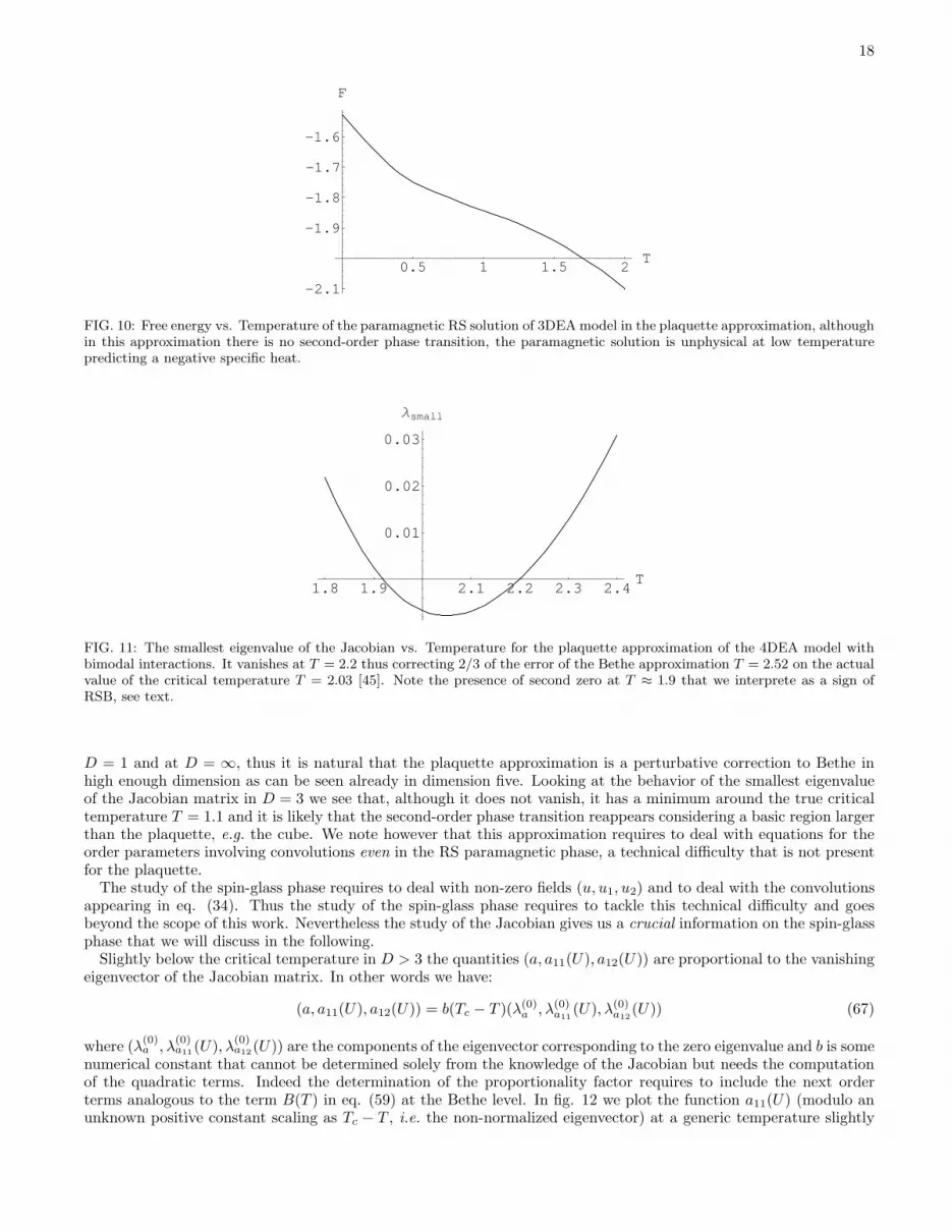
FIG. 10: Free energy vs. Temperature of the paramagnetic RS solution of 3DEAmodel in the plaquette approximation, althoughin this approximation there is no second-order phase transition, the paramagnetic solution is unphysical at low temperaturepredicting a negative specific heat.

1.8 1.9 2.1 2.2 2.3 2.4T

0.01

0.02

0.03

Λsmall

FIG. 11: The smallest eigenvalue of the Jacobian vs. Temperature for the plaquette approximation of the 4DEA model withbimodal interactions. It vanishes at T = 2.2 thus correcting 2/3 of the error of the Bethe approximation T = 2.52 on the actualvalue of the critical temperature T = 2.03 [45]. Note the presence of second zero at T ≈ 1.9 that we interprete as a sign ofRSB, see text.

D = 1 and at D = ∞, thus it is natural that the plaquette approximation is a perturbative correction to Bethe inhigh enough dimension as can be seen already in dimension five. Looking at the behavior of the smallest eigenvalueof the Jacobian matrix in D = 3 we see that, although it does not vanish, it has a minimum around the true criticaltemperature T = 1.1 and it is likely that the second-order phase transition reappears considering a basic region largerthan the plaquette, e.g. the cube. We note however that this approximation requires to deal with equations for theorder parameters involving convolutions even in the RS paramagnetic phase, a technical difficulty that is not presentfor the plaquette.The study of the spin-glass phase requires to deal with non-zero fields (u, u1, u2) and to deal with the convolutions

appearing in eq. (34). Thus the study of the spin-glass phase requires to tackle this technical difficulty and goesbeyond the scope of this work. Nevertheless the study of the Jacobian gives us a crucial information on the spin-glassphase that we will discuss in the following.Slightly below the critical temperature in D > 3 the quantities (a, a11(U), a12(U)) are proportional to the vanishing

eigenvector of the Jacobian matrix. In other words we have:

(a, a11(U), a12(U)) = b(Tc − T )(λ(0)a , λ(0)a11(U), λ(0)a12

(U)) (67)

where (λ(0)a , λ

(0)a11(U), λ

(0)a12(U)) are the components of the eigenvector corresponding to the zero eigenvalue and b is some

numerical constant that cannot be determined solely from the knowledge of the Jacobian but needs the computationof the quadratic terms. Indeed the determination of the proportionality factor requires to include the next orderterms analogous to the term B(T ) in eq. (59) at the Bethe level. In fig. 12 we plot the function a11(U) (modulo anunknown positive constant scaling as Tc − T , i.e. the non-normalized eigenvector) at a generic temperature slightly

19

below Tc = 2.2 for the 4DEA with bimodal interactions, the proportionality factor is such that the a component ispositive, a = 0.08490.

-1 -0.5 0.5 1U

-0.15

-0.1

-0.05

0.05

a11

FIG. 12: The function a11(U) (modulo an unknown positive constant scaling as Tc−T ) at a generic temperature slightly belowTc = 2.2 for the 4DEA with bimodal interactions, see text. It is negative for some values of U meaning that the functionQ(U,u1, u2) is not positive definite.

We see that a11(U) is negative for some values of U and this is puzzling, indeed we recall that the definition ofa11(U) is:

a11(U) =

∫

Q(U, u1, u2)u21 du1 du2 (68)

thus if a11(U) is negative below the critical temperature for some U it follows that the message function Q(U, u1, u2)cannot be positive definite! The first consequence of this fact is that the function Q(U, u1, u2) cannot be interpretedas a distribution function of the messages (U, u1, u2) on a given sample: had we followed that interpretation we shouldhave concluded that the whole approach is inconsistent. In the next section we will discuss this issue in more depthand see that instead it is the naive interpretation that is actually inconsistent, in particular we will show that themessage functions Q(U, u1, u2) need not to be positive definite while the beliefs of the regions do.We mention that negative a11(U) are found also if we study the response of the system to the presence of a small

field H in the high-temperature phase. In this case we find non-zero values of (a, a11(U), a12(U)) of order O(H2) thatcan be determined inverting the Jacobian matrix and applying it to the O(H2) perturbation, and again we find thatwhile a is positive a11(U) is negative for some values of U . This effect survives in the infinite temperature limit. Inthis regime we find that at leading order the variables to be considered are a and a11 =

∫

a11(U) dU and an explicitcomputation shows that a ≃ H2β2 and a11 ≃ −3β6H2 in any dimension.We note that the fact that the messages are not positive definite means that they cannot be simply represented as

populations and this, together with the presence of convolutions in the variational equations, is a technical challengeto be overcome in order to obtain quantitative results for general CVM approximations and for all regions of thephase diagram.We also mention that the Jacobian approach presented here can be also applied to study the phase diagram of

models with ferromagnetically biased interactions, in this case one would be interest in the location of the ferromagnetictransition and the variables to be used should be a =

∫

q(u)u du and a1(U) =∫

Q(U, u1, u2)u1du1du2dU .We end this section with a comment on the peculiar feature displayed by the smallest eigenvalue of the Jacobian

in four dimension according to fig. (11). Below T = 2.2 we expect to find a RS spin-glass solution with a non-zeropositive value of a ∝ (Tc−T ). As we already said the actual value of the proportionality factor cannot be determinedsolely from the knowledge of the Jacobian but needs the computation of the quadratic terms. However if we assumethat these terms do not change too much with the temperature between the T = 2.2 and T = 1.9 (i.e. where theeigenvalue vanishes again) we easily see that the parameter a should have the opposite behaviour of the smallesteigenvalue. In particular, lowering the temperature, it will initially increase from zero to some maximum and thendecrease again to zero. This would be completely unphysical and means that probably to RS spin-glass solutionbecomes meaningless and has to be abandoned below some temperature greater that T = 2.05 where the smallesteigenvalue reaches its minimum. It is tempting to interprete this fact as an indication that the RS spin-glass solution isphysically wrong at low temperature and that a RSB solution has to be considered instead. One can further speculatethat if this is the case two phenomena should be observed. First the effect should become more pronounced whileincreasing the size of the basic CVM region. In other words increasing the precision of the CVM approximation the

20

region of validity of the RS spin-glass solution should shrink to zero i.e. the first two zeroes of the smallest eigenvalueshould tend to coincide. Second for a given CVM approximation the use of a RSB solution should increase the rangeof validity of the solution shifting the point where the solution becomes unphysical to lower temperatures. We thinkthat this is a very interesting open problem.

VII. PHYSICAL INTERPRETATION OF THE BELIEFS

In the previous section we have seen that the messages functions Q(U, u1, u2) of the plaquette CVM approximationin general dimension are not definite positive and cannot be interpreted as distribution functions. In this section wewill obtain the physical interpretations of the beliefs of br(σ) of the regions of the replicated model. In particular wewill show that the beliefs in the RS approximation can be interpreted as distributions over the disorder of the localHamiltonians.We consider first the belief of a point on the lattice, say 0. In the n-replicated system there are n spins σ1

0 , . . . , σn0

on that point. As we saw in section II averaging over the disorder couples the different replicas and the effectiveHamiltonian becomes −

∑

ij ln〈exp[βJ∑

a σai σ

aj ]〉. The belief b(σ0) describes the marginal distribution of the repli-

cated spins at point 0 with respect to the replica Hamiltonian. Any correlation between any number p of the n spinsat site 0 can be expressed in terms of b(σ0)

〈〈σa10 . . . σ

ap

0 〉〉 =∑

σ0

(σa10 . . . σ

ap

0 )b(σ0) (69)

where 〈〈· · · 〉〉 means average with respect to the replicated Hamiltonian. On the other hand such a correlation canbe written as:

〈〈σa10 . . . σ

ap

0 〉〉 =

∑

{σ}(σa10 . . . σ

ap

0 )〈eβ∑

ij,a Jijσai σ

aj 〉

∑

{σ}〈eβ∑

ij,a Jijσaiσaj 〉

=〈 (〈σa1

0 〉J . . . 〈σap

0 〉J)ZnJ 〉

〈ZnJ 〉

=〈mp

0,JZnJ 〉

〈ZnJ 〉

(70)

Where 〈· · · 〉 means average over the disorder, ZJ is the partition function of the non-replicated system for a givenrealization of the disorder J , 〈· · · 〉J means thermodynamic average at given disorder J and m0,J is the magnetizationat site 0 of the non-replicated system with a given disorder realization J . The equality between the second and thethird term follows from putting the disorder average outside the sum over the configurations of the replicated systemand thus recovering the independence of the different replicas prior to the averaging. The above equations tells usthat the correlation between p replicated spins at the same site 0 is equal to the average with respect of the disorderof the p moment of the magnetization at site 0 of the non-replicated system. Note that each disorder realization isweighted with a weight proportional to the partition function to the power n. In particular when n → 0 we recoverthe standard white average over the disorder while for non-zero n we are selecting samples with free energy differentfrom the typical one [31]. According to section A the RS parametrization of the belief b(σ0) is obtained through afunction p(u) (the same for each site) in the form:

b(σ0) =

∫

p(u)eβu

∑aσa0

(2 coshβu)ndu , (71)

now using eq. (69) and (70) we finally arrive at the following equation:

∫

p(u)(tanhβu)p du =〈mp

0,JZnJ 〉

〈ZnJ 〉

(72)

The above equation encodes the physical meaning of the belief function p(u). On a given sample J the magnetizationm0,J of site 0 is determined by an effective field u = arctanh(m0,J)/β on site 0 generated by the rest of the system.Since the above equation is valid for any p it follows that the function p(u) is the distribution over the different samplesof the effective field acting on a given site.The same interpretation can be obtained for the belief of the couple of points and for the plaquette. On a given

sample the effect of the rest of the system on a couple of spins σ1 and σ2 generates an effective local Hamiltonian ofthe form −(Uσ1σ2 +u1σ1+u2σ2) that determines completely the magnetizations and correlation of the two spin; thebelief function of the couple of points P (U, u1, u2) is the distribution over the different samples of the effective localHamiltonian.

21

The CVM approach (in particular eq. (5)) tells us that the distributions p(u) and P (U, u1, u2) can be expressed interms of the message functions q(u) and Q(U, u1, u2) in the following way (we specialize as before to the 2DEA modelon the regular lattice):

p(u) =

∫ 4∏

i=1

[q(ui)dui]δ(u− (u1 + u2 + u3 + u4)) (73)

and

P (U, u1, u2) =

∫ 3∏

i=1

[q(ui)dui]

3∏

i=1

[q(vi)dvi]∏

a=up,down

[Q(Ua, ua, va)dUaduadva]P (J)dJ ×

× δ(U − (Uup + Udown + J)) δ

(

u1 − (

3∑

i=1

ui + uup + udown)

)

δ

(

u2 − (

3∑

i=1

vi + vup + vdown)

)

(74)

In the Bethe approximation the message function q(u) can be interpreted as the disorder distribution of the effectivefield u on a given spin σ with connectivity c when c−1 links connected to it are removed. This is a peculiar feature ofthe Bethe approximation but in general the message functions do not admit an interpretation as distributions as theone derived above. Indeed, as we have seen in the previous section, they are not positive definite in general. On theother hand it can be argued that the distribution Pno−J(U, u1, u2) of the effective Hamiltonian of a couple of pointsin the absence of the link connecting them obeys the equation:

P (U, u1, u2) =

∫

dU ′dJPno−J(U′, u1, u2)δ(U − (U ′ + J))P (J) (75)

and therefore Pno−J(U, u1, u2) is equal to (74) without the integration over P (J)dJ :

Pno−J(U, u1, u2) =

∫ 3∏

i=1

[q(ui)dui]

3∏

i=1

[q(vi)dvi]∏

a=up,down

[Q(Ua, ua, va)dUaduadva] ×

× δ(U − (Uup + Udown)) δ

(

u1 − (

3∑

i=1

ui + uup + udown)

)

δ

(

u2 − (

3∑

i=1

vi + vup + vdown)

)

(76)

A similar expression can be obtained for the distribution of the effective Hamiltonian of the plaquette without thelinks inside it. We note that the distribution Pno−J (U, u1, u2) allows a straightforward computation of the local energythrough the following expression that can be also (consistently) obtained in way similar to eq. (72) deriving explicitlythe replicated free energy.

E = −

∫

P (J)dJPno−J (U, u1, u2)dUdu1du2Jtanh(βU + βJ) + tanhβu1 tanhβu21 + tanh(βU + βJ) tanhβu1 tanhβu2

(77)

From eqs. (73) and (74) we see that the message functions Q(U, u1, u2) and q(u) need not to be positive definite butthey must be such that p(u),P (U, u1, u2) and Pno−J(U, u1, u2) are. We will check that this is indeed the case in thefollowing. In the last section we have argued that at the critical temperature of the spin-glass phase transition thefields u are small and at first order in T − Tc the message functions are described by the variables (a, a11(U), a12(U))that represent the average of the second moments of the fields, see eq. (56) and (58). Consistently we noted thatthese variables are proportional to the eigenvector with zero eigenvalue of the Jacobian matrix and checked that theeigenvector (and thus (a, a11(U), a12(U))) is such that the function Q(U, u1, u2) cannot be positive definite, see fig.12. In the following we consider the similar quantities for P (U, u1, u2) near the critical temperature:

q11(U) ≡

∫

P (U, u1, u2)u21du1du2 (78)

q12(U) ≡

∫

P (U, u1, u2)u1u2du1du2 (79)

Given that P (U, u1, u2) is a distribution we must find q11(U) ≥ 0 and q11(U)−q12(U) ≥ 0 for all U . On the other handfrom eq. (74) we see that q11(U) and q12(U) can be obtained from (a, a11(U), a12(U)) through a linear transformation,

22

again modulo an unknown positive constant that scales as Tc−T . In fig. 13 and 14 we plot q11(U) and q11(U)−q12(U)for the 4DEA model with bimodal interactions slightly below the critical temperature, they were obtained througha linear transformation from the corresponding (a, a11(U), a12(U)), (a11(U) is shown in fig. 12). Consistently we seethat unlike a11(U), both q11(U) and q11(U)− q12(U) are positive for all U as they should. One can check that similarquantities corresponding to Pno−J(U, u1, u2) or the plaquette are also compatible with the general fact that the beliefshave to be interpreted as a distribution functions over the disorder of the local effective Hamiltonians.

-3 -2 -1 1 2 3U

0.025

0.05

0.075

0.1

0.125

0.15

0.175

q11

FIG. 13: The function q11(U) =∫P (U,u1, u2)u

2

1 du1 du2 (modulo an unknown positive constant scaling as Tc −T ) at a generictemperature slightly below Tc = 2.2 for the 4DEA with bimodal interactions, see text. It is always positive as it should sinceP (U,u1, u2) is a distribution.

-3 -2 -1 1 2 3U

0.005

0.01

0.015

0.02

0.025

0.03

0.035

q11 - q12

FIG. 14: The function q11(U)− q12(U) =∫P (U, u1, u2)(u1 − u2)

2/2 du1 du2 (modulo an unknown positive constant scaling asTc−T ) at a generic temperature slightly below Tc = 2.2 for the 4DEA with bimodal interactions, see text. It is always positiveas it should since P (U,u1, u2) is a distribution.

In the previous section we noticed that interpreting the message function Q(U, u1, u2) as a distribution of themessages (U, u1, u2) on a given instance is wrong and misleading. We have seen why it is misleading: had weinterpreted in that way we would have look for a solution in the spin-glass phase with strictly positive a11(U) whilethe true a11(U) is negative form some values of U . We conclude this section providing some arguments to show thatit is inconsistent.Consider the function for the belief of the single point eq. (73). Can we interpreter it as saying that q(u) describes

the distribution of the messages ui on a given realization of the disorder? The answer is no because it would leadto conclude that these messages are spatially uncorrelated. This is true in the Bethe approximation but not in theplaquette approximation, for instance the messages coming from the direction North and West come from regions thatare both contained in the NW plaquette and cannot be uncorrelated. Furthermore we may notice that this equationremains the same if we consider the CVM approximation in which the basic region is a generic L × L plaquette.Once again on a given instance we would have four messages entering on a point but when we average over differentsamples these messages are correlated: thus it is crucial to understand that the function q(u) has nothing to do withthe distribution of the messages on a single sample. Actually the messages are auxiliary objects of the approach whilethe true physical objects are the beliefs.

23

Similarly looking at the equation for the beliefs of the couple of points eq. (74) we see that if we interpretedQ(U, u1, u2) as the distribution over different samples of the messages fields (U, u1, u2) and q(u) as that of u, weshould have concluded that the corresponding messages are spatially uncorrelated and again we see that this is incontrast with the key CVM assumption that objects in the same basic region (the plaquette) are correlated.Finally if we go back to the definition of the messages functions we see that a generic message ρ(σ1, σ2) in terms

of replicated spins must be positive function, instead the corresponding function Q(U, u1, u2) is some kind of integraltransform of ρ(σ1, σ2) and need not to be positive.We are now in position to discuss the relationship between the replica CVM approach and the earlier results of the

Tohoku group [12–14]. In 1980 Katsura, Fujiki and Nagahara were the first to apply CVM ideas to spin-glasses andstudied the phase diagrams of various models. They started from the CVM message-passing equations on a givensample and introduced the functions q(u) and Q(U, u1, u2) intended to be the sample-to-sample distributions of themessages (actually they wrote Q(U, u1, u2) = Q(U)g(u1)g(u2)). As we discussed in section IV, these assumptionslead to the same set of equations for q(u) and Q(U, u1, u2) that we have obtained through Replica CVM at the RSlevel. However, even if the equations are the same, the starting assumptions are inconsistent and in the end theactual solutions q(u) and Q(U, u1, u2) turn out not to be distributions. Thus we think that in general Replica CVMprovides a more satisfactory and consistent derivation of the RS CVM equations obtained nearly thirty years agoby the Tohoku group. Most importantly the equations follow from a variational principle and can be generalized toinclude RSB.Actually Katsura et al. did not write down the full set of equations (33,34,35) but studied the paramagnetic solution

in various models and considered the location of a second-order spin-glass phase transition. They solved equation (38)approximating Q(U) as a couple of delta functions, then in order to locate the transition temperature they studiedthe Jacobian under the assumption that Q(U, u1, u2) = Q(U)g(u1)g(u2). This assumption is inconsistent with theequation for Q(U, u1, u2) that does not admit a factorized solution but simplifies the computation of the Jacobianbecause one has to deal with just two variables a ≡

∫

q(u)u2 du and a11 ≡∫

g(u)u2 du compared to the full set ofvariables (a, a11(U), a12(U)) of the exact plaquette CVM. As expected their results are less precise than ours, forinstance they obtained a spurious spin-glass phase transition on the 2DEA on the square lattice while remarkably wefind no second-order phase transition. On the other hand their treatment allows to obtain an analytical expression ofthe Jacobian and of the phase diagrams and they could apply it to various models.

VIII. DISCUSSION

The Replica CVM can be used in principle to study the phase diagram of a wide range of disordered systems and it isalso possible that it can be used to get quantitative predictions on single samples. However there are quantitative andqualitative technical differences with respect to standard CVM (and the GBP algorithm), to the Bethe approximationand to SP that represent a great challenge. In particular, integrals in many dimension, convolutions and messagefunctions that are not positive definite conjure to make applications extremely difficult beyond the simplest CVMapproximations and smallest number of RSB.Besides these technical difficulties the results of the second part of the paper show that, at least in the averaged

case, the method yields sound results. This is not at all trivial given the frustrated nature of the model and the trickycontinuation in replica number.In many respects the method shares the same advantages and weak points of standard CVM. It is a good tool to

obtain quantitative non-perturbative estimates in actual models and to characterize phase diagrams, e.g. the stabilityof the paramagnetic phase down to zero temperature in 2D spin-glass models is a remarkable result and we alreadymentioned that the Jacobian approach can be straightforwardly applied to study the ferromagnetic transition in 2DEA models with ferromagnetically biased interactions. Thus the method improves over perturbative schemes, say the1/D expansion that on the other hand are more tractable in order to get qualitative results on systems with full-RSB[48].On the other hand a standard CVM approximation is not guaranteed to be an upper bound to the true free energy

and like many non-perturbative approximations can possibly give inconsistent results, in this respect we note thatthe plots of the free energy suggest that a good sequence of Replica CVM approximations of increasing precisionshould approach the true free energy from below and not from above as in standard CVM. This appears to be aconsequence of the replica trick much as the fact that Parisi formula for the SK model has to be maximized and notminimized in order to determine the free energy [15]. Another drawback is that CVM is intrinsically a mean-fieldapproximation. As such it will always predict mean-field critical exponents although in principle information on thetrue critical exponent can be obtained [18] e.g. comparing approximations with maximal regions of increasing size.However the problem of going beyond mean-field theory (i.e. using the loop expansion in Replica Field Theory) is waymore important than to build more precise mean-field approximations like those yielded by replica CVM. This said

24

quantitative estimates can be rather useful to help solve long-standing problems in spin-glass theory. For instance anestimate of the actual location of the De Almeida-Thouless line [15] in finite dimensional models is highly desirable.The next step beyond the applications presented here should be the RS treatment of the spin-glass phase of the

EA model in the plaquette approximation, at least in D > 3. This include the extension to finite small n thatcan be seen as a first simplified version of 1RSB (the so-called factorized solution). On the Bethe lattice [49] thisimproves considerably the RS result and differs little from the more precise 1RSB solution [2]. A similar considerableimprovement of the factorized solution with respect to the RS one also in the plaquette approximation, if observed,would constitute non-trivial evidence supporting the RSB nature of the spin-glass phase in finite-dimensional modelsbelow the upper critical dimension 6.A way to reduce the technical complexity of the exact Replica CVM equations is to use the variational expres-

sion, eqs. (7) and (B13), of the free energy parametrizing the messages functions in a simplified way and solvingthe corresponding variational equations that will be different from the exact equations (B2,B3) and (B4,B5). Thenumber of possible parametrizations is virtually infinite, for instance it should be noted that in high-dimension theplaquette approximation can be considered a perturbative correction to the Bethe approximation and the RS functionQ(U, u1, u2) is peaked at small values of all its arguments. Therefore in that regime it is consistent to parametrizeQ(U, u1, u2) with few of its moments while considering the full q(u), the application of this ansatz to finite dimensionwould be non-perturbative but could give consistent results. A different possibility is to assume that in the wholelow-temperature phase, not only near Tc, the small fields distributions are essentially parametrized by their secondmoments, this amounts to consider as variables the functions Q(U) and the parameters (a, a11(U), a12(U)) introducedin section VI. To obtain the variational equations of this ansatz we should parametrize the distribution of the fields(U, u1, u2) as delta functions plus second derivatives of delta functions, such that all moments of order higher thantwo vanish.The main reason to look for tractable replica CVM approximations beyond the Bethe approximation is that one

could then try to apply them on single samples in the spirit of the SP algorithm. On the other hand if one is justinterested in the averaged properties it may be useful to consider also tree-like approximation with regions of increasingsize. Being tree-like they are free of the convolutions and negative message functions problems, i.e. fully treatablewith population dynamic algorithms. Therefore although they will be less precise than CVM approximations largerregions could be treated and extrapolation to the actual finite dimensional model achieved.

Acknowledgments

We thank I. Nishimori, Y. Kabashima, J. Poulter and A. Pelizzola for useful comments on the first version ofthis work. A. Lage and R. Mulet thank the hospitality of I.S.I. during the completion of this work. A. Lage alsoacknowledges support by the EC-funded STREP GENNETEC (“Genetics Networks: emergence and copmlexity”)

Appendix A: The Hierarchical Ansatz

In this appendix we present the hierarchical ansatz for the replicated CVM in full generality. In particular we willconsider: i) a general CVM approximation, ii) a general number of RSB steps, iii) both the single sample and averagedcases. In appendix B the variational equations and the variational free energy will be derived.In section III we have written the free energy in terms of messages that are positive functions of the configu-

rations xr of the variables in region r. In the following we will parametrize the messages in order to be able totake the analytical continuation to real n, the RSB parametrization requires the introduction of a set of K RSBparameters 1 ≤ x1, . . . , xK ≤ n that are numbers. Unfortunately at this stage the standard notations of the message-passing formulation of CVM [6] and of RSB [15] overlaps and the reader should not confuse the RSB parameter1 ≤ x1, . . . , xK ≤ n (that are numbers) with the xr defined previously (that specifies distinct configurations of thevariable nodes in region r). However from now on we will concentrate on the Edwards-Anderson model defined above,therefore the nodes are Ising spins, e.g. for the region comprising spin a and b we have xab ≡ {σa, σb} if the systemis not replicated and xab ≡ {σa, σb} if the system is replicated n times, such that at each site, say a, we have n spinsσa ≡ (σ1

a, . . . σna ).

The general RS and RSB ansatz of a function ρ(σ) of n spins was originally presented in [19], later its parametrizationin terms of distributions of fields was suggested in [20] and later revisited in [1], and we refer to those paper for anexplanation of the main ideas underlying it. Here we generalize it to a generic function ρ(σ1, . . . , σp) where each σi isa set of n Ising spins.We start introducing the field U that parametrize a probability distribution of p Ising spins, in the following we

call it a p-field. U is a set of 2p − 1 real numbers {uI} where I is an index that labels all the subsets of the set of

25

indices {1, . . . , p}, (the empty set is excluded). We have then:

PU (σ1, . . . , σp) = N (U) expβ

∑

i

uiσi +∑

i≤j

uijσiσj +∑

i≤j≤k

uijkσiσjσk + · · ·+ u1,...,pσ1 . . . σp

(A1)

Where N (U) is a normalization constant. We define a probability distribution (population) P (0)(U) of such fields a0-distribution, correspondingly a 1-distribution is a probability distribution on probability distributions (populationof populations) and so on. A k-distribution will be written as P (k) and it defines a measure P (k)dP (k−1) over thespace of k − 1-distributions.In order to parametrize the function ρ(σ1, . . . , σp) with K steps of RSB we need:

• a K-distribution P (K) of the fields U ;

• K integers 1 ≤ x1, . . . , xK ≤ n (for n < 1 they become real and the inequalities change sign);

In the following we will consider the parameters 1 ≤ x1, . . . , xK ≤ n fixed and consider just the dependency on thedistributions. The construction is iterative and requires a set of functions ρP (k)(σ1, . . . , σp) where each σi is a set of

xk+1 spins with k = 1, . . . ,K (we define xK+1 ≡ n and x0 ≡ 1). The normalization of ρP (k) is crucial, we choose tonormalize all of them to 1. We define ρP (k)(σ1, . . . , σp) starting from ρP (k−1)(σ1, . . . , σp) first dividing all the xk+1 × pspins in xk+1/xk groups {σ1, . . . , σp}C of xk × p spins labeled by an index C = 1, . . . , xk+1/xk. Then we have:

ρP (k)(σ1, . . . , σp) =

∫

P (k)dP (k−1)

xk+1/xk∏

C=1

ρP (k−1)({σ1, . . . , σp}C) (A2)

Thus ρ(σ1, . . . , σp) ≡ ρP (K)(σ1, . . . , σp) is defined iteratively starting from the Replica-Symmetric case correspondingto k = 0:

ρP (0)(σ1, . . . , σp) =

∫

P (0)(U)dU

x1∏

i=1

PU ({σ1, . . . , σp}i) (A3)

We will parametrize each message mrs(xs) through a population P(K)rs over a p-field where p is the number of sites

in region s. The populations associated to the tilded messages mrs defined in eq. (9) will be represented by P(K)rs .

Note that at integer values of n, the above parametrization is redundant, and in principle we cannot determine thepopulation knowing the messages. It is standard in the replica method to assume instead that this step can beperformed due to the continuation to real values of n.In the end we will write down the message-passing equations in terms of the message populations and thus we

will be able to consider non-integer values of n, and in particular the limit n → 0. We will also obtain a variationalexpression of the free energy in terms of the message populations. We note that in principle one could parametrize thebeliefs with populations and obtain an expression of Kikuchi free energy in terms of these populations. The resultingexpression however is extremely complicated due to the presence of the entropic terms in the form

∑

xrbr ln br, see e.g.

[20] where the entropy of the point belief was computed. The main reason why we derived the variational expression(7) in terms of the messages is precisely because it avoids to deal with terms of the form

∑

xrbr ln br.

The r.h.s. of the rescaled iteration equation (10) defines a function mrs of the messages in M(r) \M(s). Now since

the messages are parametrized by K-populations, we need to determine the corresponding function P(K)rs that yields

a K-population as a function of the K-populations of the messages, such that the iteration equation translates into

P(K)rs = P

(K)rs .

We start introducing two J-dependent functions mJ,rs and NJ,rs such that the following equation is satisfied:

mJ,rsNJ,rs =∑

xr\s

ψJr\s(xr)

∏

mr′′s′′∈M(r)\M(s)

mr′′s′′ (A4)

We use bold face for indicating functions of messages, but we stress that while mJ,rs returns a normalized probability

on spins in region s, the function NJ,rs returns a number which is precisely the normalization required by equation

(A4). This equation can be written in terms of populations and defines a K-population P(K)J,rs as a function of the

K-populations in M(r) \M(s). It turns out that the function P(K)J,rs can be defined in terms of the function P

(K−1)J,rs

26

that in turn can be defined through the function P(K−2)J,rs and so on. The resulting expression for a given k is:

P(k)J,rs =

1

N(k)J,rs

∫

∏

mr′′s′′∈M(r)\M(s)

P(k)r′′s′′dP

(k−1)r′′s′′

[N(k−1)J,rs ]xk+1/xkδ(P (k−1)

rs − P(k−1)J,rs ) (A5)

where N(k)J,rs is a number that is a function of the k-populations P

(k)r′′s′′ in M(r) \M(s) defined according to:

N(k)J,rs ≡

∫

∏

mr′′s′′∈M(r)\M(s)

P(k)r′′s′′dP

(k−1)r′′s′′

[N(k−1)J,rs ]xk+1/xk . (A6)

In the cavity formulation at the Bethe level [1] the quantities N(k)J,rs are associated to (cluster) free energy shifts and

they appear in (A5) as reweighting terms. At the Bethe level, explicit expressions like (A5) for any k value have beenalready reported in Ref. [50].The iterative definition must be supplemented with the two functions for k = 0 and k = −1. They reads:

P(0)J,rs =

1

N(0)J,rs

∫

∏

mr′′s′′∈M(r)\M(s)

P(0)r′′s′′dUr′′s′′

[N(−1)J,rs ]

x1δ(Urs − UJ,rs) (A7)

and

N(0)J,rs ≡

∫

∏

mr′′s′′∈M(r)\M(s)

P(0)r′′s′′dUr′′s′′

[N(−1)J,rs ]

x1 (A8)

For x1 = n this yields the Replica-Symmetric solution, note that in this case in the n→ 0 limit the reweighting term

goes to 1 and is irrelevant. In the above equations Urs and N(−1)rs are functions of the fields Ur′′s′′ that have to be

obtained solving the following single-replica equation:

ρUJ,rs

(σs)N(−1)J,rs =

∑

{σr\s}

ψJr\s(σr)

∏

mr′′s′′∈M(r)\M(s)

ρUr′′s′′(σs′′ ) (A9)

Note that it is only at this stage that the actual properties of the model enter. This complete the recursive definition

of the function P(k)J,rs and N

(k)J,rsthat solve equation (A4) at any level of k-RSB, we will not write down the proof of

this statement that can be worked out iteratively generalizing a similar derivation in the Bethe approximation [21].It is important to stress that this iterative definition is possible only if we do not average over the disorder, a passagethat will be taken in the next section.Up to now we have expressed eq. (10) in terms of populations in such a way that the n→ 0 limit can be taken, in

the following we consider the similar treatment for eq. (9). Note the basic differences between eq. (9) and (10): theabsence of the summation over the spins in region r \ s and the fact that we consider messages in M(r, s) and not inM(r) \M(s).

Much as above, the function Q(k)rs corresponding to the r.h.s. of eq. (9) can be defined in an recursive way, the

result being:

Q(k)rs =

1

M(k)rs

∫

P (k)rs dP

(k−1)rs

∏

mr′′s′′∈M(r,s)

P(k)r′′s′′dP

(k−1)r′′s′′

[M(k−1)rs ]xk+1/xkδ(P (k−1)

rs − Q(k−1)rs ) (A10)

where M(k)rs is defined as:

M(k)rs ≡

∫

P (k)rs dP

(k−1)rs

∏

mr′′s′′∈M(r,s)

P(k)r′′s′′dP

(k−1)r′′s′′

[M(k−1)rs ]xk+1/xk . (A11)

As before the previous iterative definition is completed specifying the two function at the Replica-Symmetric levelcorresponding to k = 0:

Q(0)rs =

1

M(0)rs

∫

P (0)rs dUrs

∏

mr′′s′′∈M(r,s)

P(0)r′′s′′dUr′′s′′

[M(−1)rs ]x1δ(Urs − Q(−1)

rs ) (A12)

27

and

M(0)rs ≡

∫

P (0)rs dUrs

∏

mr′′s′′∈M(r,s)

P(0)r′′s′′dUr′′s′′

[M(−1)rs ]x1 . (A13)

For x1 = n this gives back the Replica-Symmetric solution, note that in this case in the n → 0 limit the reweightingterm goes to 1.

The two quantities Q(−1)rs and M

(−1)rs have the following form that does not depend on the Hamiltonian of the

problem:

Q(−1)rs ≡ Urs +

∑

mr′′s′′∈M(r,s)

Ur′′s′′ (A14)

The above sum is intended in vectorial form, i.e. for each possible combination of the spins in region s(σi,σiσj ,σiσjσk . . . ) we sum the corresponding fields. The normalization factor can be written as the productof terms depending on each message separately times a term depending on the sum of the fields:

M(−1)rs ≡

N (Urs)∏

mr′′s′′∈M(r,s) N (Ur′′s′′ )

N (Q(−1)rs )

(A15)

The above properties have important consequences and allow to introduce Fourier-like transforms in order to writedown the equations for the messages in explicit form, see appendix C.

Appendix B: Generalized Survey Propagation Equations

We are now in position to write the variational equations (6) in terms of K-populations. We start noticing that inthe averaged case eq. (10) can be written as:

mrsC = 〈mJ,rsNJ,rs〉J (B1)

where C is a normalization constant. The r.h.s. of the previous equation is a linear combination of spin probabilitiesand it is easy to see that the corresponding K-population is just a linear combination of the corresponding K-populations with same coefficients NJ,rs and the normalization factor is just that sum of the coefficients i.e. 〈NJ,rs〉J .

The populations corresponding to mJ,rs are given by eq. (A5) and we see that the coefficients NJ,rs in eq. (B1)

cancel the term at the denominator in (A5), thus the resulting equation for the populations P(K)rs is:

P (K)rs =

1

〈N(K)J,rs〉J

∫

∏

mr′′s′′∈M(r)\M(s)

P(K)r′′s′′dP

(K−1)r′′s′′

〈[N(K−1)J,rs ]xK+1/xK δ(P (K−1)

rs − P(K−1)J,rs )〉J (B2)

P (K)rs = Q(K)

rs (B3)

Note that in the limit n → 0 we have N(K)rs → 1 because xK+1 = n. These equations are translationally invariant,

meaning that the populations P(K)rs does not depends on where regions r and s are actually on the lattice but just

on their shape and mutual positions with respect to each other. For instance in the Bethe approximation we have asingle K-population that does not fluctuate over the sites. The right hand sides of the above equations (B2) and (B3)should be thought of as respectively the r.h.s. and l.h.s. of a single equation that in general involves the messages

populations P(K)rs in implicit form. This is the main difference with respect to the Bethe approximation where the

messages appears in explicit form and the equations can be solved iteratively, a discussion of these equations in thecontext of the CVM plaquette approximation will be given at the end of next section.On a single sample instead the distributions fluctuate over the sites. As a consequence the solution with K-RSB

steps is parametrized by (K − 1)-RSB populations fluctuating over space. The corresponding equations are:

P (K−1)rs = P

(K−1)J,rs (B4)

28

P (K−1)rs = Q(K−1)

rs (B5)

For instance the 1-RSB solution on a given sample is described by populations of fields that fluctuate over differentregions. Again the right hand sides of the above equations (B4) and (B5) should be thought of as respectively ther.h.s. and l.h.s. of a single equation that in general involves the messages in implicit form.When K = 1 and the maximal region is the couple of points (i.e. we work in the Bethe approximation) the above

equations reproduce the celebrated Survey Propagation (SP) equations [1–4], hence the name Generalized SurveyPropagation equations. The SP equations were originally obtained through the cavity method, while a derivation ofthe SP equations on a single sample using replicas was obtained in [51].

1. The Free Energy and its Derivatives

The variational expression of the free energy eq. (7) can be written in terms of populations along the same lines ofthe previous sections. The results in the averaged case is:

FK = −∑

r∈R

cr ln〈N(K)J,r 〉J (B6)

where N(K)J,r is a J-dependent function of the K-Populations corresponding to the messages in M(r) that can be

defined iteratively in terms of the populations as:

N(k)J,r =

∫

∏

r′′s′′∈M(r)

P(k)r′′s′′dP

(k−1)r′′s′′ (N

(k−1)J,r )xk+1/xk (B7)

with

N(0)J,r =

∫

∏

r′′s′′∈M(r)

P(0)r′′s′′dUr′′s′′(N

(−1)J,r )x1 (B8)

where

N(−1)J,r =

∑

{σr}

ψJr (σr)

∏

r′′s′′∈M(r)

ρUr′′s′′(σs′′ ) (B9)

On a single instance instead we have:

FK = −∑

r∈R

cr lnN(K−1)J,r (B10)

where the N(K−1)J,r have to be evaluated in terms of the K− 1-populations entering region r. In order to make explicit

the similarity with the cavity formulation of [1] we define a new function

∆F(k)J,r ≡ −

1

βxk+1lnN

(k)J,r (B11)

Consequently the above quantity has again a recursive definition:

∆F(k)J,r = −

1

βxk+1ln

∫

∏

r′′s′′∈M(r)

P(k)r′′s′′dP

(k−1)r′′s′′ e

−βxk+1∆F(k−1)J,r (B12)

with this definition we have:

Φ(n) = −1

βnN

∑

r∈R

cr ln〈e−βn∆F

(K)J,r 〉J (B13)

and

f = limn→0

Φ(n) =1

N

∑

r∈R

cr

∫

∏

r′′s′′∈M(r)

P(K)r′′s′′dP

(K−1)r′′s′′ 〈∆F

(K−1)J,r 〉J (B14)

29

In the average case the message populations do not fluctuate over space and the contribution of each region of a givenform to the free energy is the same. Thus the sum over all regions can be replaced by the sum of the contributionsof the basic types of regions r each multiplied by the number nr of regions of type r per spin. For instance in theplaquette approximation of the 2D square lattice we have cplaquette = 1, ccouple = −1 and cpoint = 1, and the numberof regions per spin are respectively nplaquette = 1, ncouple = 2 and npoint = 1.It is also important to determine the derivatives of the free energy with respect to the parameters 1 ≤ x1, . . . , xK ≤ n

[1, 2]. Since the above expression is variational with respect to the populations the total derivative of the free energywith respect to xk coincides with its partial derivative with respect to xk.Clearly in order to determine the derivative of the free energy with respect to the parameters 1 ≤ x1, . . . , xK ≤ n

we only need to determine the derivatives of the function ∆F(K)J,r . The derivative of ∆F

(p)J,r with respect to xp+1 is:

∂xp+1∆F(p)J,r = −

1

xp+1∆F

(p)J,r + 〈〈∆F

(p−1)J,r 〉〉

(p)J,r (B15)

where we have defined:

〈〈. . . 〉〉(k)J,r =

∫∏

r′′s′′∈M(r) P(k)r′′s′′dP

(k−1)r′′s′′ . . . e−βxk+1∆F

(k−1)J,r

∫ ∏

r′′s′′∈M(r) P(k)r′′s′′dP

(k−1)r′′s′′ e

−βxk+1∆F(k−1)J,r

(B16)

Then the derivative ∂xp+1∆F(K)J,r can be obtained using the recursive definition. Indeed we see that the derivatives of

∆F(k)J,r for k > p with respect to xp+1 parameters obey the following recursive equation:

∂xp+1∆F(k)J,r = 〈〈∂xp+1∆F

(k−1)J,r 〉〉

(k)J,r for k > p (B17)

For instance in the 1RSB case in the n→ 0 limit we get a similar result to Ref. [1]:

∂f1RSB

∂x1=∑

r∈R

cr

∫

∏

r′′s′′∈M(r)

P(1)r′′s′′dP

(0)r′′s′′

(

−1

x1〈∆F

(0)J,r〉J + 〈 〈〈∆F

(−1)J,r 〉〉

(0)J,r 〉J

)

(B18)

2. From populations to functionals

In the preceding sections we have worked under the assumption that the messages and the beliefs are bothparametrized through populations of populations of fields. In section IV we have applied the approach to the EAmodel on various lattices in the CVM plaquette approximation. We made the simplest non-trivial ansatz, i.e. theRS ansatz, that we expect to be good in the high-temperature paramagnetic phase. On a single sample the messagesare just numbers in the RS phase, and the corresponding equations are the GBP equations of [6]. For the replicatedaveraged system instead the messages according to the above parametrization should be distributions of fields. As wehave seen it turns out that the actual solution requires to consider messages parametrized by functions that are notpositive definite i.e. that are not distributions. This tells us that in practice when solving a given model we may beforced to consider parametrization of the form (A2) where instead of populations of fields we should consider functionsof the fields, or instead of populations of populations we should consider functionals. At any rate, it is easily seen thatthe equations obeyed by these objects do not change at all depending on whether they are distributions or functions

i.e. all the results of the previous subsection hold. On the other hand it can be argued that the function N(k)J,rs defined

above should always give a positive number and this is guaranteed only if it is a function of k-populations, therefore itappears that in any case we should parametrize a message at level K of RSB with a function of K−1-populations andthis function may eventually be non-positive definite. In other words it seems to us that we can relax the conditionto use distributions only at the last level of RSB.

Appendix C: The Inversion Problem

The generalized survey propagation equations derived previously express the tilded populations in terms of thenon-tilded ones. To obtain an explicit expression for the message functions one needs to invert equations (B3) (oreq. (B5) on a given sample) and obtain an expression for the non-tilded populations in terms of the tilded ones. Atthe lowest RSB levels, (i.e. RS in the averaged case and 1RSB on a single sample) this can be done using Fourier

30

transforms. In this appendix we will show that at any number K of RSB steps the inversion can be achieved inprinciple using appropriate integral transforms of the populations. An algorithm able to go back and forth from thepopulations to their transforms would provide a route to the numerical solution of the Generalized Survey Propagationequations but unfortunately an efficient implementation seems quite difficult.Basically we will work with nested Fourier transform, i.e. Fourier transforms of Fourier transforms. We will

introduce the invertible integral transform T(k)rs of a k-population P

(k)rs and show that eq. (B3) in terms of transform

reads:

T (k)rs = T (k)

rs +∑

mr′′s′′∈M(r,s)

T(k)r′′s′′ (C1)

From the previous expression we can easily compute T(k)rs from T

(k)rs . Again we will proceed iteratively, showing that

if the previous equation is valid at level k − 1 it is also valid at level k. In order to do this we also assume that it

exists a function G(k−1) such that the quantity M(k−1)rs can be written as

M(k−1)rs =

G(k−1)(T(k−1)rs )

∏

mr′′s′′∈M(r,s) G(k−1)(T

(k−1)r′′s′′ )

G(k−1)(T(k−1)rs )

(C2)

where T(k−1)rs ) in the above equation is computed as the sum of the non-tilded transform. We can write eq. (A10) in

terms of the transforms at level k − 1:

Q(k)rs (T

(k)rs )(T (k−1)

rs ) =1

M(k)rs

∫

P (k)rs (T (k−1)

rs )dT (k−1)rs

∏

mr′′s′′∈M(r,s)

P(k)r′′s′′(T

(k−1)r′′s′′ )dT

(k−1)r′′s′′

[M(k−1)rs ]xk+1/xk ×

× δ

T (k−1)rs − T (k−1)

rs −∑

mr′′s′′∈M(r,s)

T(k−1)r′′s′′

(C3)

now using eq. (C2) we can redistribute the reweighting term between the various populations and rewrite the previousequation as:

Q(k)rs (G(k−1)

rs )xk+1/xk =1

M(k)rs

∫

P (k)rs (G(k−1)

rs )xk+1/xkdT (k−1)rs

∏

mr′′s′′∈M(r,s)

P(k)r′′s′′(G

(k−1)r′′s′′ )xk+1/xkdT

(k−1)r′′s′′

×

× δ

T (k−1)rs − T (k−1)

rs −∑

mr′′s′′∈M(r,s)

T(k−1)r′′s′′

(C4)

In the previous equation Q(k)rs (G

(k−1)rs )xk+1/xk defines a measure over the space of k−1 transform. We Fourier transform

the previous equation with respect to the k − 1 transform and obtain:

F (k)rs =

1

M(k)rs

F (k)rs

∏

mr′′s′′∈M(r,s)

F(k)r′′s′′ (C5)

accordingly the factor M(k)rs can be obtained as the transform evaluated at a given value, e.g. zero argument; this

yields:

M(k)rs =

F(k)rs (0)

∏

mr′′s′′∈M(r,s) F(k)r′′s′′ (0)

F(k)rs (0)

(C6)

Now we can take the logarithm of the previous equation and define:

T (k)rs ≡ ln

F(k)rs

F(k)rs (0)

(C7)

we see that with this definition eq. (C1) is satisfied at level k. Correspondingly eq. (C2) is also satisfied provided weidentify the function G with:

G(k)rs ≡ F (k)

rs (0) (C8)

31

To complete the proof we need to show that eq. (C1) and eq. (C2) are valid at k = 0, the replica symmetric case. To

do this we easily see that eqs. (A14) and (A15) have this structure. Therefore at the RS level the transform T(0)rs is

defined as:

T(0)(rs)(Srs) = ln

∫

P(0)rs (Urs)N (Urs)

x1dUrs exp iSrsUrs∫

P(0)rs (Urs)N (Urs)x1dUrs

(C9)

and we have:

G(0)rs =

∫

P (0)rs (Urs)N (Urs)

x1dUrs (C10)

Summarizing, at the RS level, the integral transform needed to solve the inversion problem is defined as the logarithmof the Fourier transform of the reweighted distribution of fields. Note that if the solution is purely RS we have x1 = nand the reweighting term is absent in the n → 0 limit. From the above RS expression one can go to 1RSB using eq.(C7). At 1RSB the solution is parametrized by a population of populations, and the transform is the logarithm ofthe Fourier transform of the reweighted distribution of the logarithm of the Fourier transforms of the populations.

[1] M. Mezard and G. Parisi, Eur. Phys. J. B 20, 217 (2001).[2] M. Mezard and G. Parisi, J. Stat. Phys 111, 1 (2003).[3] M. Mezard and R. Zecchina, Phys. Rev. E 66, 056126 (2002).[4] M. Mezard, G. Parisi and R. Zecchina, Science 297, 812 (2002).[5] Y. Kabashima and D. Saad, Europhys. Lett. 44, 668-674 (1998).[6] J.S. Yedidia, W.T. Freeman and Y. Weiss, Advances in Neural Information Processing Systems (NIPS) 13, 689 (2000).[7] J.S. Yedidia, W.T. Freeman and Y. Weis, IEEE Transactions on Information Theory 51, 2282, (2005).[8] R. Kikuchi, Phys. Rev. 81, 988 (1951). T. Morita, M. Suzuki, K. Wada and M. Kaburagi (eds.): Foundations and

Applications of Cluster Variation Method and Path Probability Method, Prog. Theor. Phys. Suppl. 115 (1994).[9] A.K. Hartmann and A.P. Young, Phys. Rev. B 64, 180404(R) (2001).

[10] T. Jorg, J. Lukic, E. Marinari and O.C. Martin, Phys. Rev. Lett. 96, 237205 (2006).[11] H.G. Ballesteros et al., Phys. Rev. B 61, 3215 (2000).[12] S. Katsura and S. Fujiki, J. Phys. C: Solid St. Phys., 13 (1980) 4711.[13] S. Fujiki and S. Katsura, J. Phys. C: Solid St. Phys., 13 (1980) 4723.[14] S. Katsura and I. Nagahara, J. Phys. C: Solid St. Phys., 13 (1980) 4995.[15] M. Mezard, G. Parisi, and M.A. Virasoro, Spin glass theory and beyond, World Scientific (Singapore 1987).[16] A. Crisanti, G. Paladin, H.-J. Sommers and A. Vulpiani, J. Phys. I France 2, 1325 (1992).[17] G. Parisi and T. Rizzo, Phys. Rev. Lett. 101, 117205 (2008).[18] A. Pelizzola, J. Phys. A 38, R309 (2005).[19] Y. Goldschmidt and C. De Dominicis, Phys. Rev. B 41, 2186 (1989).[20] R. Monasson, J. Phys. A 31, 513 (1998).[21] G. Parisi and T. Rizzo, Large Deviations of the Free-Energy in Diluted Mean-Field Spin-Glass, J. Phys. A. in press.[22] M. Ohzeki and H. Nishimori, preprint arXiv:0905.3623v1.[23] R.G. Palmer and J. Adler, Int. J. Mod. Phys. C 10, 667 (1999).[24] I.A. Campbell, A.K. Hartmann and H.G. Katzgraber, Phys. Rev. B 70, 054429 (2004).[25] S. Boettcher, Phys. Rev. B 67, 060403 (2003); Eur. Phys. J. B 31, 29 (2003).[26] J.A. Blackman, J.R. Goncalves and J. Poulter, Phys. Rev. E 58, 1502 (1998).[27] J. Lukic, A. Galluccio, E. Marinari, O.C. Martin and G. Rinaldi, Phys. Rev. Lett. 92, 117202 (2004).[28] A. Pelizzola, Phys. Rev. B 61, 11510 (2000)[29] J. Poulter and J.A. Blackman, J. Phys. A 34, 7527 (2001).[30] A. Aromsawa, Ph.D. Thesis, Mahidol University (2007).[31] G. Parisi and T. Rizzo, Phys. Rev. B 79, 134205 (2009).[32] T. Aspelmeier, A. Billoire, E. Marinari and M.A. Moore (2008) J. Phys. A: Math. Theor. 41 324008.[33] J.-P. Bouchaud, F. Krzakala and O.C. Martin, Phys. Rev. B 68, 224404 (2003).[34] J. Wehr and M. Aizenman, J. Stat. Phys. 60, 287 (1990).[35] T. Temesvari, The Ising spin glass in finite dimensions: a perturbative study of the free energy, arXiv:0911.0362[36] T. Aspelmeier and M.A. Moore, Phys. Rev. Lett. 90, 177201 (2003).[37] J.-S. Wang and R. H. Swendsen, Phys. Rev. B 38, 4840 (1988).[38] L. Saul and M. Kardar, Phys. Rev. E 48, R3221 (1993); Nucl. Phys. B 432, 641 (1994).[39] J.-S. Wang, Phys. Rev. E 72, 036706 (2005).[40] H.G. Katzgraber, L.W. Lee and I.A. Campbell, cond-mat/0510668 (2005).[41] W. Atisattapong and J. Poulter, New J. Phys. 10, 093012 (2008).

32

[42] H.G. Katzgraber, L.W. Lee and I.A. Campbell, Phys. Rev. B 75, 014412 (2007).[43] W. Atisattapong and J. Poulter, preprint arXiv:0901.1538 (2009).[44] A. Pelizzola, M. Pretti, Phys. Rev. B 60, 10134 (1999).[45] E. Marinari and F. Zuliani, J. Phys. A: Math. Gen. 32, 7447 (1999).[46] L. Klein, J. Adler, A. Aharony, A.B. Harris and Y. Meir, Phys. Rev. B 43, 11249 (1991).[47] D. Daboul, I. Chang and A. Aharony, Eur. Phys. J. B 41, 231 (2004).[48] A. Georges, M. Mezard and J.S. Yedidia, Phys. Rev. Lett. 64, 2937 (1990).[49] Y.Y. Goldschmidt and P.-Y.Lai, J. Phys. A 23, L775 (1990).[50] G. Semerjian, J. Stat. Phys. 130, 251 (2008).[51] Y. Kabashima, J. Phys. Soc. Jpn. 74, 2133 (2005).[52] The original name was “Cluster Variation Method”, but we believe “Cluster Variational Method” to be a better wording.[53] We adopt the original notation of Ref. [6], which was changed in the more recent Ref. [7]. The ensembles M(r) \ M(s)

and M(r, s) corresponds respectively to N(r, s) and M(r, s) defined in [7]. Note however that for us these are ensembles ofcouples of regions labels instead of ensembles of the corresponding messages as in [6].

[54] Actually one obtain a different set of equations that can be proved to be equivalent to eqs. (6) along the same lines of theproof that the two sets of constraints are equivalent, see theorem 5 in [7]