a SpringerOpen Journal

Severino et al. SpringerPlus 2014, 3:493http://www.springerplus.com/content/3/1/493

RESEARCH Open Access

Dynamic cluster scheduling for cluster-treeWSNsRicardo Severino*, Nuno Pereira and Eduardo Tovar

Abstract

While Cluster-Tree network topologies look promising for WSN applications with timeliness and energy-efficiencyrequirements, we are yet to witness its adoption in commercial and academic solutions. One of the arguments thathinder the use of these topologies concerns the lack of flexibility in adapting to changes in the network, such as intraffic flows.This paper presents a solution to enable these networks with the ability to self-adapt their clusters’ duty-cycle andscheduling, to provide increased quality of service to multiple traffic flows. Importantly, our approach enables anetwork to change its cluster scheduling without requiring long inaccessibility times or the re-association of thenodes. We show how to apply our methodology to the case of IEEE 802.15.4/ZigBee cluster-tree WSNs withoutsignificant changes to the protocol. Finally, we analyze and demonstrate the validity of our methodology through acomprehensive simulation and experimental validation using commercially available technology on a StructuralHealth Monitoring application scenario.

Keywords: Cluster-tree networks; Message scheduling; Quality-of-service in WSN

IntroductionThe increasing tendency for the integration of computa-tions with physical processes at large scale has been push-ing research on new paradigms for networked embeddedsystems design (Stankovic et al. 2005). In this line, Wire-less Sensor Networks (WSNs) have naturally emerged asenabling infrastructures for these cyber-physical applica-tions due to their potential to closely interact with externalstimulus. Applications such as homeland security, healthcare, building or factory automation are just a few elu-cidative examples of how these emerging technologies willimpact our daily life and society at large.Given the large number of these WSN applications,

each with an individual set of requirements (Raman andChebrolu 2008), it is important that some of these WSNresources (e.g. bandwidth and buffer size), are predicted inadvance, in order to support the prospective applicationswith a pre-defined Quality-of-Service (QoS). To achievethis, it is mandatory to rely on structured logical topolo-gies such as cluster-trees (e.g. (Abdelzaher et al. 2004,Gibson et al. 2007, Prabh and Abdelzaher 2007)), which

*Correspondence: rar@isep.ipp.ptCISTER Research Centre, ISEP/IPP, Rua Antonio Bernardino de Almeida 431,4200-072 Porto, Portugal

provide deterministic behaviour instead of flat mesh-liketopologies, where QoS guarantees are difficult to provide,if not impossible.Nevertheless, although these network topologies look

promising for the above mentioned WSN applications,there is a lack of flexibility in adapting to changes inthe traffic or bandwidth requirements at run-time, mak-ing them not capable of allocating more bandwidth to aset of nodes sensing a particular phenomena, or reduc-ing the latency of a data stream. In fact, although there isalready some literature on how to compute these networkresources (Jurcik et al. 2010, Hanzalek and Jurcik 2010), itis not clear how they could be re-allocated without greatlyinterfering with the network functionality, and speciallywithout imposing high inaccessibility times.This paper presents a solution to this problem, enabling

networks to change at run-time a given initial schedule,based on a time-division strategy, to provide increasedquality of service to multiple traffic flows. Computingthis would normally result in a complex integer program-ming problem which would be infeasible to be computedby WSN nodes which typically have scarce computingpower. Our re-scheduling algorithm relies on a heuris-tic that can be easily computed in these platforms. We

© 2014 Severino et al.; licensee Springer. This is an Open Access article distributed under the terms of the Creative CommonsAttribution License (http://creativecommons.org/licenses/by/4.0), which permits unrestricted use, distribution, and reproductionin any medium, provided the original work is properly credited.

Severino et al. SpringerPlus 2014, 3:493 Page 2 of 17http://www.springerplus.com/content/3/1/493

show how to apply our methodology to the particular caseof IEEE 802.15.4/ZigBee, good candidates to enable thiskind of networks. Finally, we analyze and demonstratethe validity of our methodology through a comprehen-sive simulation study and experimental validation usingWSN platforms in a real-world Structural Health Moni-toring scenario. Our proposal can reduce the end-to-endlatency by 93% and the overall data stream transmit periodby 49%, although higher values can be achieved underdifferent network settings.

Related workIn general, synchronized Cluster-Tree topologies tend tosuffer from four technical issues that usually preventtheir use: (1) how to schedule the transmissions of differ-ent neighbouring clusters avoiding interference; (2) howto predict the performance limits to correctly allocateresources; (3) how to change the resource allocation ofthe Cluster-tree (CT) on-the-fly; and (4) the lack of avail-able and functional implementations over standard WSNtechnologies, such as the IEEE 802.15.4/ZigBee set ofprotocols.There is already an interesting body of work concern-

ing the scheduling of general tree-based WSNs. Most ofthe work addresses the case of minimizing the length ofTDMA-based schedules for improved convergecast (Choiet al. 2009, Lai et al. 2008). In (Gandham et al. 2008), a dis-tributed algorithm is proposed in contrast with previousmore centralized solutions. Recently, in (Incel et al. 2012) ascheduling strategy is combined with transmission powercontrol to minimize collision between nodes, and a strat-egy to schedule transmissions in different frequencies isalso proposed.Although these strategies might work for a pure

TDMA-based tree, cluster-based trees impose a differentapproach since each slot of the TDMA cycle is usuallynot allocated to one single node, but to a cluster withmany nodes, and often nodes which are contending formedium access, thus rendering most delay bound resultsnot significant. This greatly reduces the number of appli-cation scenarios for such proposals, considering currentstandardization trends.This is especially true for the particular case of the

IEEE 802.15.4/ZigBee set of protocols, in which althoughthe Cluster-Tree network topology is supported, no cleardescription on how to implement it is given, namely inwhat concerns the beacon collision problem. In (Std. IEEE802.15.4 2006), theTaskGroup 15.4b proposed some basicapproaches to solve this: the beacon-only period approachand the time division approach, only to be removed in the2006 revision.In this line, a few proposals were made targeting the

scheduling of ZigBee cluster-tree networks. The work in(Pan and Tseng 2008) introduced the Minimum Delay

Beacon Scheduling problem, however this proposal onlyaddressed the latency problem and not the bandwidthproblem, since it assumed the use of GTS slots for con-vergecast. The work in (Jurcik et al. 2010), addresses theproblem of predicting resource needs by modelling theperformance limits of a ZigBee CT network using GTSflows. In another proposal (Hanzalek and Jurcik 2010),the authors extend the previous work by computing theoptimal schedule for several GTS data flows. Recently,(Di Francesco et al. 2012) followed a similar approach to(Pan and Tseng 2008), proposing two heuristics to reducethe complexity of the otherwise NP-complete problem.Although the usage of GTS guarantees real-time per-formance within the IEEE802.15.4/ZigBee standards, thenumber of available GTS slots is quite limited as well astheir bandwidth. In this line, in (Huang et al. 2012) theauthors try to overcome this by borrowing bandwidthfrom neighbouring nodes.All of the above proposals work by computing a static

schedule, based on periodic traffic assumptions, whichwill remain active throughout the network lifetime. More-over, they follow a purely theoretical approach, lacking aclear description on how to implement such mechanismson ZigBee. In fact, in some cases it is arguable if it is evenpossible.For instance, the work in (Huang et al. 2012) pro-

poses the concept of adoptive-parents, something whichis clearly not compliant with the ZigBee protocol. Sim-ilarly, two other proposals (Yeh et al. 2008) and (Danet al. 2010), try to improve routing efficiency and decreaselatency by proposing important changes to the basis ofthese standards. The first by proposing a change to thesuperframe structure to encompass two active periodsper Cluster-Head, the second, by proposing a completelynew tree-routing protocol for ZigBee. In (Kim et al. 2007)the authors propose yet another non-compliant way ofreducing the schedule latency by passing frames to neigh-bouring clusters, changing a cluster-tree topology into amesh by supporting multiple paths. Moreover, allowinginter-cluster messaging leads to interference and eventu-ally beacon collision problems, since nodes do not knowthe neighbouring cluster’s active periods. In (Toscano andLo Bello 2009) the authors use different radio channels toavoid tackling the problem.It is clear that standard communication technologies

able to support tree-based topologies, could benefit fromfull-compliant scheduling mechanisms. To make this areality, proposals should as much as possible, presentclear implementation details, showing how to enable theirusage within current communication standards. In theseauthors’ opinion, in addition to simulation, carrying outexperimental validations of such mechanisms over real-world platforms is mandatory when addressing theseprotocols.

Severino et al. SpringerPlus 2014, 3:493 Page 3 of 17http://www.springerplus.com/content/3/1/493

In this line, in (Koubaa et al. 2007), the Time DivisionCluster Schedule (TDCS) algorithm was proposed andimplemented in the Open-ZB stack (Cunha et al. 2007)enabling for the first time the use of this topology overIEEE 802.15.4/ZigBee based networks, guaranteeing nobeacon collisions. This technique used a time-divisionapproach and worked by assigning a different time off-set to each cluster. Fully implemented over commer-cial WSN platforms, available to the TinyOS community(TinyOS 2014), and with a set of network planning toolsavailable to the general WSN community via Open-ZB(Open-ZB 2014), we believe this work to be a provenreference concerning beacon scheduling for CT ZigBeenetworks. Other proposals followed a similar approachsuch as (Burda and Wietfeld 2007) for mesh networks, or(Muthukumaran et al. 2010).Although some literature on solving the first two afore-

mentioned problems in this section is already available,none of the proposals so far, in the general case of syn-chronized Cluster-Trees, addresses the third one, at leastin a satisfactory way, and guaranteeing standard com-pliance. This greatly limits the flexibility of the networkwhich must keep the same cluster schedule and band-width reservation, independently of the flow of data inthe network and of its particular requirements, whichdepending on the application may certainly change. Inthis paper, we propose a set of techniques in which thebase schedule is temporary changed to encompass tran-sient networking necessities such as end-to-end delay andbandwidth allocation. This work, already presented in(Severino et al. 2013a), is now extended with new experi-mental results obtained over a real-world structural healthmonitoring application and significantmore detail is givento the proposal and its implementation over the IEEE802.15.4/ZigBee standards.

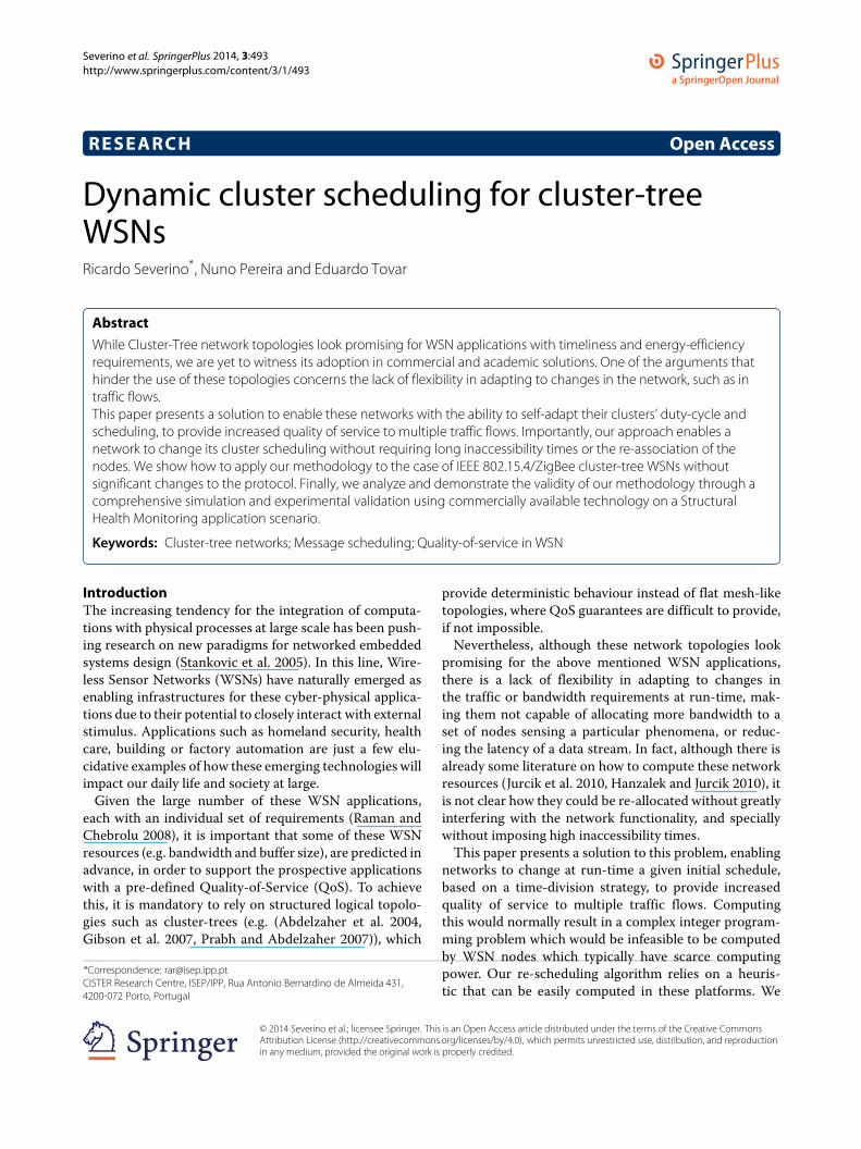
SystemmodelConsider a synchronized cluster-tree WSNs featuring atree-based logical topology where nodes are organized indifferent groups, called clusters. Each node is connectedto a maximum of one node at the lower depth, calledparent node, and can be connected to multiple nodes atthe upper depth, called child nodes (by convention, treesgrow down). Each node only interacts with its pre-definedparent and child nodes.A cluster-tree topology contains two main types of

nodes: routers and end-nodes (refer to Figure 1). Thenodes that can associate to previously associated nodesand can participate in multi-hop routing are referred toas routers. The leaf nodes that do not allow association ofother nodes and do not participate in routing are referredto as end-nodes. The router that has no parent is calledroot and it might hold special functions such as identifi-cation, formation and control of the entire network. Note

that the root is at depth zero. Both routers and end-nodescan have sensing capabilities, therefore they are generallyreferred to as sensor nodes. Each router forms its clusterand is referred to as cluster-head of this cluster (e.g. routerC11 is the cluster-head of cluster 11). Each cluster-headis also responsible for synchronization in its cluster andperiodically sends synchronization frames. All child nodes(i.e. end-nodes and routers) of a cluster-head are associ-ated to its cluster, and the cluster-head handles all theirdata transmissions. It results that each router (except theroot) belongs to two clusters, once as a child and once asa parent (i.e., a cluster-head). A schedule of the clusters tominimize or eliminate inter-cluster interference, follow-ing a time-division strategy is assumed to be already inplace.In general, the radio channel is a shared communica-

tion medium where more than one node can transmit atthe same time. In cluster-tree WSNs, messages are for-warded from cluster to cluster until reaching the sink.The time window of each cluster is periodically dividedinto an active portion (AP), during which the cluster-headenables data transmissions inside its cluster, and a sub-sequent inactive portion, during which all cluster nodesmay enter low-powermode to save energy resources.Notethat each router must be awake during its active portionand the active portion of its parent router. To avoid col-lisions between clusters, it is mandatory to schedule theclusters’ active portions in an ordered sequence, that wecall TDCS so that no inter-cluster collision occurs. Incase of single collision domain, the TDCS must be non-overlapping, i.e. only one cluster can be active at any time.Hence, the duration of the TDCS’s cycle is given by thenumber of clusters and the length of their active por-tions. On the contrary, in a network with multiple colli-sion domains, the clusters from different non-overlappingcollision domains may be active at the same time. How-ever, finding a TDCS that avoids clusters’ collisions ina large-scale WSN with multiple collision domains is aquite complex problem, hence in this paper, for sim-plification, we always assume a single collision domain.For more information concerning TDCS, please refer to(Koubaa et al. 2007).Several data transmissions in an upstream direction

(e.g. streams S1, S2, S3 in Figure 1) can be present inthe network simultaneously. Each stream is noted as atuple Sk =< Rk , Pk ,Tk ,Dk >, where, Rk represents theordered set of clusters which the stream k must cross toreach the sink, Pk represents the priority for that stream(an integer from 0 to 5), Tk represents the number ofTDCS cycles for which stream k will remain active andDk the depth of the stream’s source. This stream nota-tion will be used in the next section to support thecomputation of a better TDCS schedule to apply to thenetwork.

Severino et al. SpringerPlus 2014, 3:493 Page 4 of 17http://www.springerplus.com/content/3/1/493

Figure 1 Systemmodel.

Dynamic cluster schedulingWith TDCS (Koubaa et al. 2007), it is possible to findthe best schedule for the routers active periods in orderto avoid interference, and to support most of the net-work bandwidth requirements. However, the schedule isdone at network setup time and assumes a static net-work that will remain unchanged. The choice of the TDCSschedule has a strong impact on the end-to-end delays.In fact, it is easy to observe that in a single collisiondomain, where there are no overlapping clusters, a TDCSschedule optimized for downstream communication willresult in the worst-case for upstream communication,and consequently in higher end-to-end delays. More-over, routers are assigned with a fixed bandwidth theymight not always need, while other clusters might be lack-ing. We aim at reacting to different data flow changeson-the-fly, while simultaneously minimizing the networkinaccessibility time. Our proposal achieves this via twotechniques: (1) re-ordering the clusters’ active periods tofavour one set of streams, reducing the end-to-end delays,which we call DCR (Dynamic Cluster Re-ordering); and(2) tuning the size of the clusters’ duration, increasing thebandwidth of the clusters serving a specific stream, aneventually decreasing others’ bandwidth, whichwe namedDBR (Dynamic Bandwidth Re-allocation). The first tech-nique consists of a rescheduling of the clusters order inthe TDCS cycle, aiming at minimizing end-to-end delays,

while the second technique consists on rearranging thebandwidth allocation for the clusters involved in a stream,to increase its bandwidths and decrease the overall timefor a data stream transmission. Both techniques can beused together, or separately. Importantly, the mechanismpresents a complexity of O(N), where N represents thenumber of Cluster-Heads in the network, making it suit-able to be run overWSN platforms with scarce processingpower. This low complexity also avoids a much largerenergy depletion of the central node in charge of runningDCS.

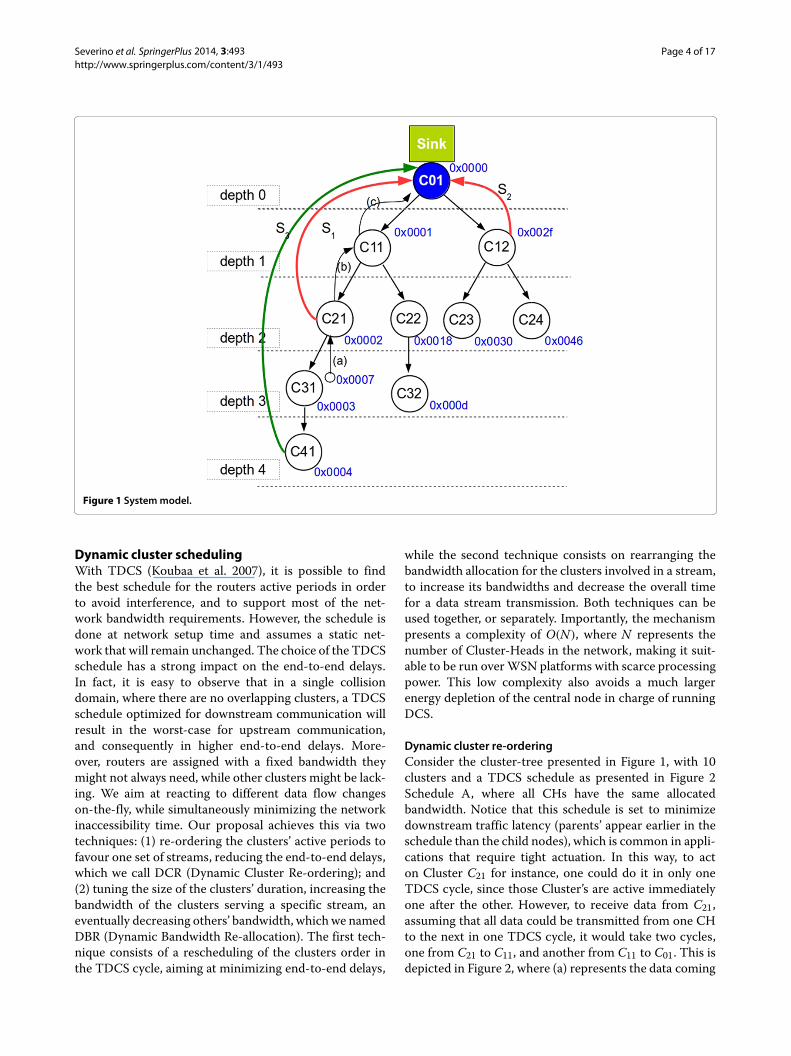
Dynamic cluster re-orderingConsider the cluster-tree presented in Figure 1, with 10clusters and a TDCS schedule as presented in Figure 2Schedule A, where all CHs have the same allocatedbandwidth. Notice that this schedule is set to minimizedownstream traffic latency (parents’ appear earlier in theschedule than the child nodes), which is common in appli-cations that require tight actuation. In this way, to acton Cluster C21 for instance, one could do it in only oneTDCS cycle, since those Cluster’s are active immediatelyone after the other. However, to receive data from C21,assuming that all data could be transmitted from one CHto the next in one TDCS cycle, it would take two cycles,one from C21 to C11, and another from C11 to C01. This isdepicted in Figure 2, where (a) represents the data coming

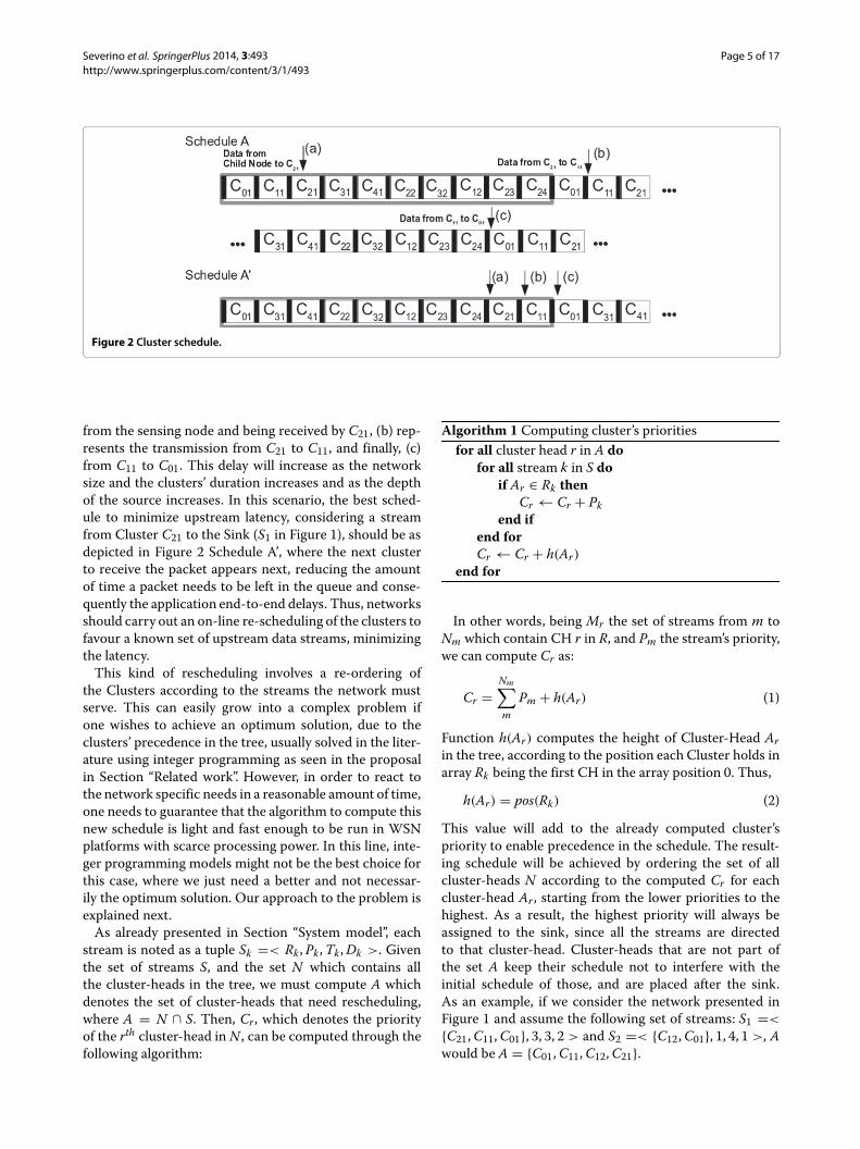
Severino et al. SpringerPlus 2014, 3:493 Page 5 of 17http://www.springerplus.com/content/3/1/493

Figure 2 Cluster schedule.

from the sensing node and being received by C21, (b) rep-resents the transmission from C21 to C11, and finally, (c)from C11 to C01. This delay will increase as the networksize and the clusters’ duration increases and as the depthof the source increases. In this scenario, the best sched-ule to minimize upstream latency, considering a streamfrom Cluster C21 to the Sink (S1 in Figure 1), should be asdepicted in Figure 2 Schedule A’, where the next clusterto receive the packet appears next, reducing the amountof time a packet needs to be left in the queue and conse-quently the application end-to-end delays. Thus, networksshould carry out an on-line re-scheduling of the clusters tofavour a known set of upstream data streams, minimizingthe latency.This kind of rescheduling involves a re-ordering of

the Clusters according to the streams the network mustserve. This can easily grow into a complex problem ifone wishes to achieve an optimum solution, due to theclusters’ precedence in the tree, usually solved in the liter-ature using integer programming as seen in the proposalin Section “Related work”. However, in order to react tothe network specific needs in a reasonable amount of time,one needs to guarantee that the algorithm to compute thisnew schedule is light and fast enough to be run in WSNplatforms with scarce processing power. In this line, inte-ger programming models might not be the best choice forthis case, where we just need a better and not necessar-ily the optimum solution. Our approach to the problem isexplained next.As already presented in Section “System model”, each

stream is noted as a tuple Sk =< Rk , Pk ,Tk ,Dk >. Giventhe set of streams S, and the set N which contains allthe cluster-heads in the tree, we must compute A whichdenotes the set of cluster-heads that need rescheduling,where A = N ∩ S. Then, Cr, which denotes the priorityof the rth cluster-head in N , can be computed through thefollowing algorithm:

Algorithm 1 Computing cluster’s prioritiesfor all cluster head r in A do

for all stream k in S doif Ar ∈ Rk then

Cr ← Cr + Pkend if

end forCr ← Cr + h(Ar)

end for

In other words, being Mr the set of streams from m toNm which contain CH r in R, and Pm the stream’s priority,we can compute Cr as:

Cr =Nm∑

mPm + h(Ar) (1)

Function h(Ar) computes the height of Cluster-Head Arin the tree, according to the position each Cluster holds inarray Rk being the first CH in the array position 0. Thus,

h(Ar) = pos(Rk) (2)

This value will add to the already computed cluster’spriority to enable precedence in the schedule. The result-ing schedule will be achieved by ordering the set of allcluster-heads N according to the computed Cr for eachcluster-head Ar , starting from the lower priorities to thehighest. As a result, the highest priority will always beassigned to the sink, since all the streams are directedto that cluster-head. Cluster-heads that are not part ofthe set A keep their schedule not to interfere with theinitial schedule of those, and are placed after the sink.As an example, if we consider the network presented inFigure 1 and assume the following set of streams: S1 =<

{C21,C11,C01}, 3, 3, 2 > and S2 =< {C12,C01}, 1, 4, 1 >, Awould be A = {C01,C11,C12,C21}.

Severino et al. SpringerPlus 2014, 3:493 Page 6 of 17http://www.springerplus.com/content/3/1/493

The first stream, originates at cluster C21 and has prior-ity 3, while the second, originates at cluster C12 and haspriority 1. If no reschedule was done, and assuming idealcommunication without errors and delays imposed by theMAC layers, we would expect that one packet of S1 wouldtake approximately 18 times the duration of one activeportion of a CH to reach the sink (Figure 2 Schedule A),and from S2 three active portions. If we use the presentedalgorithm it will result in the following: C01 = P1 + P2 +h(A01) = 3+ 1+ 2 = 6; C11 = P1 + h(A11) = 3+ 1 = 4;C12 = P2 + h(A12) = 1 + 1 = 2; C21 = P1 + h(A21) =3 + 0 = 3; Ordering from the lowest to the highest pri-ority, the CHs in A should be ordered as C12,C21,C11 andfinally C01.Considering the remaining nodes, which maintain their

initial order in the schedule and lowest priority, the finalschedule, would be as described in Figure 3.It would now be possible a full data transaction from

the origin cluster to the sink in one TDCS cycle, reducingthe delay of each packet, greatly benefiting applicationswhich demand low latencies. If we wanted to decreasethe latency for S2 we could increase the priority of thestream to the same of S1 or higher. This would result inC12 = P1 + h(A12) = 3 + 1 = 4, and now, C12 wouldhave a higher priority than C21 thus appearing later in theschedule, decreasing the latency.Comparing this schedule with the original in Figure 2

Schedule A, we observe that the other CHs also changedplace in the schedule. Changing the position of all nodesmust be done because there is no free room that will letus only change the streaming CHs’ position and accom-modate their initial positions unoccupied. However, thisdoes not mean that all of the CHs changed the offsetto their parents. For instance, in this particular case C41does not change the offset. This is obvious, since the dis-tance between C41 and its parent C31 did not change. Asa rule of thumb, a new offset will have to be computedfor every children one depth bellow a re-scheduled CH.For their grand-children, this does not happen since thedistance remains the same as in the original schedule.This principle will be used later in STEP 4 (Section "TheDCS communication protocol"), to compute the network’sinaccessibility time.Although this approach solves the latency problem, it

does not reduce the overall time it will take for a streamto be transmitted since there is no change to the avail-able bandwidth per cycle. Hence our second proposal,DBR, which will increase the bandwidth for the clustersinvolved in the stream.

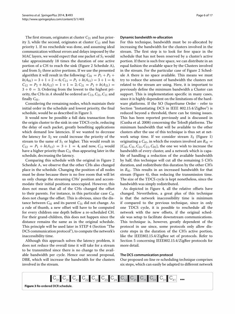
Dynamic bandwidth re-allocationFor this technique, bandwidth must be re-allocated byincreasing the bandwidth for the clusters involved in thestream. The first step is to look for free space in theschedule that has not been reserved by a cluster’s activeportion. If there is such free space, we can distribute in anequal fashion the available space by the Clusters involvedin the stream. For the particular case of Figure 2 Sched-ule A there is no space available. This means we musttry to reduce the amount of bandwidth the clusters notrelated to the stream are using. Here, it is important topreviously define the minimum bandwidth a Cluster cansupport. This is implementation specific in many cases,since it is highly dependent on the limitations of the hard-ware platforms. If the SO (Superframe Order - refer toSection "Instantiating DCS in IEEE 802.15.4/ZigBee") isreduced beyond a threshold, there can be timing issues.This has been reported previously and is discussed in(Cunha et al. 2008) concerning the TelosB platforms. Theminimum bandwidth that will be available to the otherclusters after the use of this technique is thus set at net-work setup time. If we consider stream S3 (Figure 1)originating a C41, in which the routers involved are R41 ={C41,C31,C21,C11,C01}, the one we wish to increase thebandwidth of every cluster, and a network which is capa-ble of handling a reduction of the available bandwidthby half, this technique will cut all the remaining 5 CH’sduration, and redistribute this duration by the other CH’sin R41. This results in an increased bandwidth for thatstream (Figure 4), thus reducing the transmission time.The size of the TDCS cycle is kept nonetheless, since thebandwidth was simply redistributed.As depicted in Figure 4, all the relative offsets have

changed. Nevertheless, a great plus of this techniqueis that the network inaccessibility time is minimumif compared to the previous technique, since in onlyone TDCS cycle, it is possible to reschedule all thenetwork with the new offsets, if the original sched-ule was setup to facilitate downstream communications.This technique is, however, greatly dependent of theprotocol in use since, some protocols only allow dis-crete steps in the duration of the CH’s active portion,like the IEEE802.15.4/ZigBee set of protocols. Refer toSection 5 concerning IEEE802.15.4/ZigBee protocols formore detail.

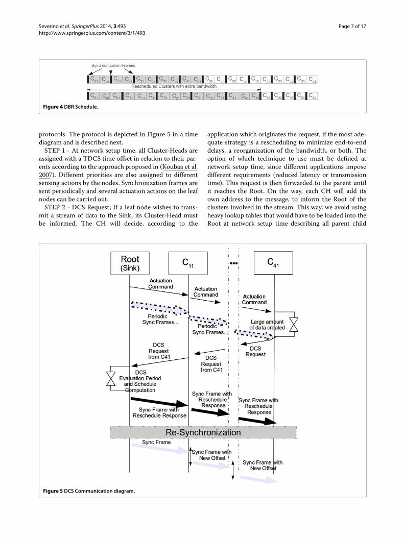
The DCS communication protocolOur proposed on-line re-scheduling technique comprisessix steps, which can easily be adapted to different network

Figure 3 Re-ordered DCR schedule.

Severino et al. SpringerPlus 2014, 3:493 Page 7 of 17http://www.springerplus.com/content/3/1/493

Figure 4 DBR Schedule.

protocols. The protocol is depicted in Figure 5 in a timediagram and is described next.STEP 1 - At network setup time, all Cluster-Heads are

assigned with a TDCS time offset in relation to their par-ents according to the approach proposed in (Koubaa et al.2007). Different priorities are also assigned to differentsensing actions by the nodes. Synchronization frames aresent periodically and several actuation actions on the leafnodes can be carried out.STEP 2 - DCS Request; If a leaf node wishes to trans-

mit a stream of data to the Sink, its Cluster-Head mustbe informed. The CH will decide, according to the

application which originates the request, if the most ade-quate strategy is a rescheduling to minimize end-to-enddelays, a reorganization of the bandwidth, or both. Theoption of which technique to use must be defined atnetwork setup time, since different applications imposedifferent requirements (reduced latency or transmissiontime). This request is then forwarded to the parent untilit reaches the Root. On the way, each CH will add itsown address to the message, to inform the Root of theclusters involved in the stream. This way, we avoid usingheavy lookup tables that would have to be loaded into theRoot at network setup time describing all parent child

Figure 5 DCS Communication diagram.

Severino et al. SpringerPlus 2014, 3:493 Page 8 of 17http://www.springerplus.com/content/3/1/493

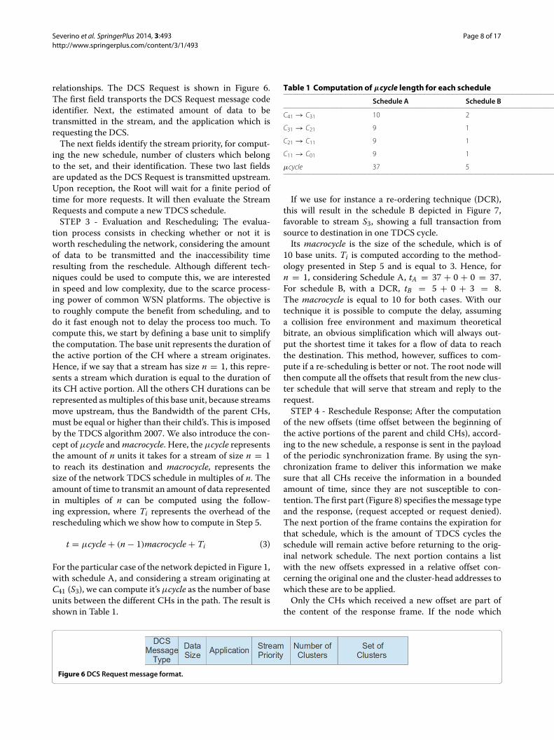
relationships. The DCS Request is shown in Figure 6.The first field transports the DCS Request message codeidentifier. Next, the estimated amount of data to betransmitted in the stream, and the application which isrequesting the DCS.The next fields identify the stream priority, for comput-

ing the new schedule, number of clusters which belongto the set, and their identification. These two last fieldsare updated as the DCS Request is transmitted upstream.Upon reception, the Root will wait for a finite period oftime for more requests. It will then evaluate the StreamRequests and compute a new TDCS schedule.STEP 3 - Evaluation and Rescheduling; The evalua-

tion process consists in checking whether or not it isworth rescheduling the network, considering the amountof data to be transmitted and the inaccessibility timeresulting from the reschedule. Although different tech-niques could be used to compute this, we are interestedin speed and low complexity, due to the scarce process-ing power of common WSN platforms. The objective isto roughly compute the benefit from scheduling, and todo it fast enough not to delay the process too much. Tocompute this, we start by defining a base unit to simplifythe computation. The base unit represents the duration ofthe active portion of the CH where a stream originates.Hence, if we say that a stream has size n = 1, this repre-sents a stream which duration is equal to the duration ofits CH active portion. All the others CH durations can berepresented asmultiples of this base unit, because streamsmove upstream, thus the Bandwidth of the parent CHs,must be equal or higher than their child’s. This is imposedby the TDCS algorithm 2007. We also introduce the con-cept of µcycle andmacrocycle. Here, the µcycle representsthe amount of n units it takes for a stream of size n = 1to reach its destination and macrocycle, represents thesize of the network TDCS schedule in multiples of n. Theamount of time to transmit an amount of data representedin multiples of n can be computed using the follow-ing expression, where Ti represents the overhead of therescheduling which we show how to compute in Step 5.

t = µcycle+ (n− 1)macrocycle+ Ti (3)

For the particular case of the network depicted in Figure 1,with schedule A, and considering a stream originating atC41 (S3), we can compute it’sµcycle as the number of baseunits between the different CHs in the path. The result isshown in Table 1.

Table 1 Computation ofµcycle length for each schedule

Schedule A Schedule B

C41 → C31 10 2

C31 → C21 9 1

C21 → C11 9 1

C11 → C01 9 1

µcycle 37 5

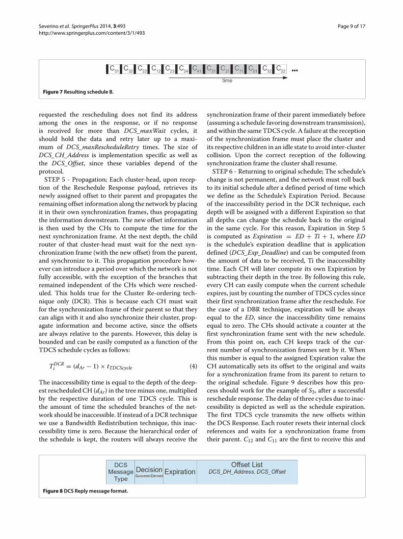
If we use for instance a re-ordering technique (DCR),this will result in the schedule B depicted in Figure 7,favorable to stream S3, showing a full transaction fromsource to destination in one TDCS cycle.Its macrocycle is the size of the schedule, which is of

10 base units. Ti is computed according to the method-ology presented in Step 5 and is equal to 3. Hence, forn = 1, considering Schedule A, tA = 37 + 0 + 0 = 37.For schedule B, with a DCR, tB = 5 + 0 + 3 = 8.The macrocycle is equal to 10 for both cases. With ourtechnique it is possible to compute the delay, assuminga collision free environment and maximum theoreticalbitrate, an obvious simplification which will always out-put the shortest time it takes for a flow of data to reachthe destination. This method, however, suffices to com-pute if a re-scheduling is better or not. The root node willthen compute all the offsets that result from the new clus-ter schedule that will serve that stream and reply to therequest.STEP 4 - Reschedule Response; After the computation

of the new offsets (time offset between the beginning ofthe active portions of the parent and child CHs), accord-ing to the new schedule, a response is sent in the payloadof the periodic synchronization frame. By using the syn-chronization frame to deliver this information we makesure that all CHs receive the information in a boundedamount of time, since they are not susceptible to con-tention. The first part (Figure 8) specifies themessage typeand the response, (request accepted or request denied).The next portion of the frame contains the expiration forthat schedule, which is the amount of TDCS cycles theschedule will remain active before returning to the orig-inal network schedule. The next portion contains a listwith the new offsets expressed in a relative offset con-cerning the original one and the cluster-head addresses towhich these are to be applied.Only the CHs which received a new offset are part of

the content of the response frame. If the node which

Figure 6 DCS Request message format.

Severino et al. SpringerPlus 2014, 3:493 Page 9 of 17http://www.springerplus.com/content/3/1/493

Figure 7 Resulting schedule B.

requested the rescheduling does not find its addressamong the ones in the response, or if no responseis received for more than DCS_maxWait cycles, itshould hold the data and retry later up to a maxi-mum of DCS_maxRescheduleRetry times. The size ofDCS_CH_Address is implementation specific as well asthe DCS_Offset, since these variables depend of theprotocol.STEP 5 - Propagation; Each cluster-head, upon recep-

tion of the Reschedule Response payload, retrieves itsnewly assigned offset to their parent and propagates theremaining offset information along the network by placingit in their own synchronization frames, thus propagatingthe information downstream. The new offset informationis then used by the CHs to compute the time for thenext synchronization frame. At the next depth, the childrouter of that cluster-head must wait for the next syn-chronization frame (with the new offset) from the parent,and synchronize to it. This propagation procedure how-ever can introduce a period over which the network is notfully accessible, with the exception of the branches thatremained independent of the CHs which were resched-uled. This holds true for the Cluster Re-ordering tech-nique only (DCR). This is because each CH must waitfor the synchronization frame of their parent so that theycan align with it and also synchronize their cluster, prop-agate information and become active, since the offsetsare always relative to the parents. However, this delay isbounded and can be easily computed as a function of theTDCS schedule cycles as follows:

TDCRi = (dAr − 1)× tTDCScycle (4)

The inaccessibility time is equal to the depth of the deep-est rescheduledCH (dAr) in the tree minus one, multipliedby the respective duration of one TDCS cycle. This isthe amount of time the scheduled branches of the net-work should be inaccessible. If instead of a DCR techniquewe use a Bandwidth Redistribution technique, this inac-cessibility time is zero. Because the hierarchical order ofthe schedule is kept, the routers will always receive the

synchronization frame of their parent immediately before(assuming a schedule favoring downstream transmission),and within the same TDCS cycle. A failure at the receptionof the synchronization frame must place the cluster andits respective children in an idle state to avoid inter-clustercollision. Upon the correct reception of the followingsynchronization frame the cluster shall resume.STEP 6 - Returning to original schedule; The schedule’s

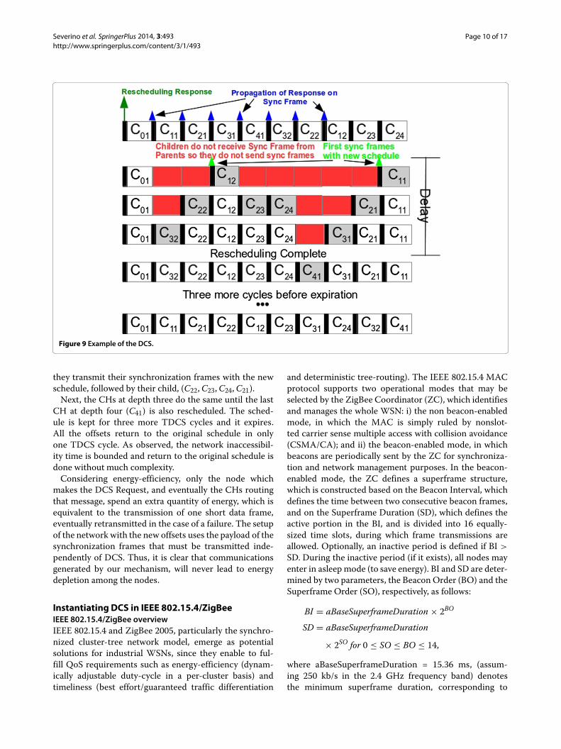
change is not permanent, and the network must roll backto its initial schedule after a defined period of time whichwe define as the Schedule’s Expiration Period. Becauseof the inaccessibility period in the DCR technique, eachdepth will be assigned with a different Expiration so thatall depths can change the schedule back to the originalin the same cycle. For this reason, Expiration in Step 5is computed as Expiration = ED + Ti + 1, where EDis the schedule’s expiration deadline that is applicationdefined (DCS_Exp_Deadline) and can be computed fromthe amount of data to be received, Ti the inaccessibilitytime. Each CH will later compute its own Expiration bysubtracting their depth in the tree. By following this rule,every CH can easily compute when the current scheduleexpires, just by counting the number of TDCS cycles sincetheir first synchronization frame after the reschedule. Forthe case of a DBR technique, expiration will be alwaysequal to the ED, since the inaccessibility time remainsequal to zero. The CHs should activate a counter at thefirst synchronization frame sent with the new schedule.From this point on, each CH keeps track of the cur-rent number of synchronization frames sent by it. Whenthis number is equal to the assigned Expiration value theCH automatically sets its offset to the original and waitsfor a synchronization frame from its parent to return tothe original schedule. Figure 9 describes how this pro-cess should work for the example of S3, after a successfulreschedule response. The delay of three cycles due to inac-cessibility is depicted as well as the schedule expiration.The first TDCS cycle transmits the new offsets withinthe DCS Response. Each router resets their internal clockreferences and waits for a synchronization frame fromtheir parent. C12 and C11 are the first to receive this and

Figure 8 DCS Reply message format.

Severino et al. SpringerPlus 2014, 3:493 Page 10 of 17http://www.springerplus.com/content/3/1/493

Figure 9 Example of the DCS.

they transmit their synchronization frames with the newschedule, followed by their child, (C22,C23,C24,C21).Next, the CHs at depth three do the same until the last

CH at depth four (C41) is also rescheduled. The sched-ule is kept for three more TDCS cycles and it expires.All the offsets return to the original schedule in onlyone TDCS cycle. As observed, the network inaccessibil-ity time is bounded and return to the original schedule isdone without much complexity.Considering energy-efficiency, only the node which

makes the DCS Request, and eventually the CHs routingthat message, spend an extra quantity of energy, which isequivalent to the transmission of one short data frame,eventually retransmitted in the case of a failure. The setupof the network with the new offsets uses the payload of thesynchronization frames that must be transmitted inde-pendently of DCS. Thus, it is clear that communicationsgenerated by our mechanism, will never lead to energydepletion among the nodes.

Instantiating DCS in IEEE 802.15.4/ZigBeeIEEE 802.15.4/ZigBee overviewIEEE 802.15.4 and ZigBee 2005, particularly the synchro-nized cluster-tree network model, emerge as potentialsolutions for industrial WSNs, since they enable to ful-fill QoS requirements such as energy-efficiency (dynam-ically adjustable duty-cycle in a per-cluster basis) andtimeliness (best effort/guaranteed traffic differentiation

and deterministic tree-routing). The IEEE 802.15.4 MACprotocol supports two operational modes that may beselected by the ZigBee Coordinator (ZC), which identifiesand manages the whole WSN: i) the non beacon-enabledmode, in which the MAC is simply ruled by nonslot-ted carrier sense multiple access with collision avoidance(CSMA/CA); and ii) the beacon-enabled mode, in whichbeacons are periodically sent by the ZC for synchroniza-tion and network management purposes. In the beacon-enabled mode, the ZC defines a superframe structure,which is constructed based on the Beacon Interval, whichdefines the time between two consecutive beacon frames,and on the Superframe Duration (SD), which defines theactive portion in the BI, and is divided into 16 equally-sized time slots, during which frame transmissions areallowed. Optionally, an inactive period is defined if BI >

SD. During the inactive period (if it exists), all nodes mayenter in asleep mode (to save energy). BI and SD are deter-mined by two parameters, the Beacon Order (BO) and theSuperframe Order (SO), respectively, as follows:

BI = aBaseSuperframeDuration × 2BO

SD = aBaseSuperframeDuration

× 2SO for 0 ≤ SO ≤ BO ≤ 14,

where aBaseSuperframeDuration = 15.36 ms, (assum-ing 250 kb/s in the 2.4 GHz frequency band) denotesthe minimum superframe duration, corresponding to

Severino et al. SpringerPlus 2014, 3:493 Page 11 of 17http://www.springerplus.com/content/3/1/493

SO = 0. During the SD, nodes compete for medium accessusing slotted CSMA/CA in the CAP. For time-sensitiveapplications, IEEE 802.15.4 enables the definition of acontention-free period (CFP) within the SD, by the alloca-tion of guaranteed time slots (GTSs). Low duty-cycles areachieved by setting small values of the superframe order(SO) as compared to the beacon order (BO), leading tolonger sleeping (inactive) periods.ZigBee defines network and application layer services

on top of the IEEE 802.15.4 protocol. In the cluster-treemodel, all nodes are organized in a parent-child rela-tionship, network synchronization is achieved through adistributed beacon transmission mechanism and a deter-ministic tree routing mechanism is used. A ZigBee net-work is composed of three device types: (i) the ZigBeeCoordinator (ZC), which identifies the network and pro-vides synchronization services through the transmissionof beacon frames containing the identification of the PANand other relevant information; ii) the ZigBee Router(ZR), which has the same functionalities as the ZC withthe exception that it does not create its own PAN-a ZRmust be associated to the ZC or to another ZR, provid-ing local synchronization to its cluster (child) nodes viabeacon frame transmissions; and (iii) the ZigBee End-Device (ZED), which neither has coordination nor routingfunctionalities and is associated to the ZC or to a ZR.

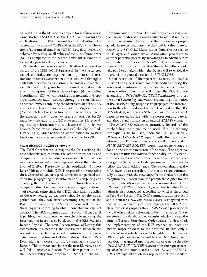
Integrating DCS in a ZigBee networkThe PAN-Coordinator is responsible for receiving thenew schedule request from the other cluster-heads andcomputing the new schedule as described before. A newmodule was devised to be integrated above the networklayer of ZigBee (Figure 10), at the Application SupportLayer. This newmodule, DCS, is responsible formanagingtheDCSmechanism, in regards to the beacon payload cre-ation (for propagating offset information), computing andchanging the offset information for the lower layers, andcomputing the schedules and corresponding expiration.At network setup time, the TDCS algorithm is applied

to the tree, setting up the base schedule. As the nodesgather data, they can direct streaming requests at thePAN Coordinator. The PAN-Coordinator will evaluatethese requests according to what is described in Step 3 ofSection “The DCS communication protocol”. If the resultis positive, it will compute the new schedule and setup theRescheduling Response to be placed in the IEEE 802.15.4Beacon Payload. The next Beacon frame will carry thisinformation. As Beacons are transmitted between theseveral clusters, the new schedule information is propa-gated among the tree and all the nodes will know a DCSRescheduling is occurring just by parsing the receivedBeacon. This is important since in the next BI, many nodeswill fail to receive a Beacon from their parent, due tothe inaccessibility time described in Step 4 of the DCS

Communication Protocol. This will be specially visible inthe deepest nodes of the rescheduled branch. If no infor-mation concerning the status of the process was propa-gated, the nodes could assume they had lost their parent,receiving a SYNC-LOSS.indication from the respectiveMAC layer, and would try an Association procedure toanother potential parent. By knowing this in advance, theycan disable this process for (Depth − 1) ∗ BI amount oftime, which is the maximum time the rescheduling shouldtake per Depth, after which, the Device will re-enable there-association procedure after the SYNC-LOSS.Upon reception of their parent’s Beacon, the ZigBee

Cluster-Heads, will search for their address among theRescheduling information at the Beacon Payload to learnthe new offset. Then, they will trigger the DCS Modulegenerating a DCS-NEW-SCHEDULE.indication, and settheir own Beacon Payload with the remaining informationof the Rescheduling Response to propagate the informa-tion to the children down the tree. Having done this, theDCS Module, will issue a SYNC.request to the NetworkLayer to resynchronize with the corresponding parent,and after a synchronization anMLME-START.request.The MLME-START.request primitive, depends of the

rescheduling technique to be used. If a Re-orderingtechnique is to be used, then the CH will used aDCS-RESTART-ROUTER.request, with the new offsetinformation. This new interface is similar the standardNLME-RESTART-ROUTER.request, except no change isdone to the other parameters of the stack. The objectiveis to simply turn the routing functionality on. If a Band-width reallocation is to be done, then the request will alsochange the Superframe Order parameter of the stack toreflect the bandwidth change. The system timers at theMAC layer, upon reception of this request are automati-cally updated with the new Superframe Order. Upon thereception of a Beacon from the parent, the ZigBee Routerwill automatically resynchronize and resume its work.When the DCS Module is triggered, the Schedule Expi-

ration is also computed according to what is describedin Step 6 of Section “The DCS communication protocol”,and a counter (DCS-Expiration-timer) is triggered withthat value. When this counter expires, the DCS Mod-ule automatically repeats theDCS-RESTART processwiththe old offset values, returning to the initial values. Theseare stored in a database, DCS-Initdb, which contains theinitial offset and Superframe Order values. As described,the implementation of the DCS mechanism does notinvolve major changes to the protocol. In fact, only acouple of new interfaces are to be added to the ZigBeeNWK implementation to enable the DCS functionali-ties. One is triggered upon reception of a new schedule(DCS-RESTART-ROUTER.request) after the regular pars-ing of a beacon frame, and another (NLME-RESTART-ROUTER.request) which is a replication of the standard

Severino et al. SpringerPlus 2014, 3:493 Page 12 of 17http://www.springerplus.com/content/3/1/493

Figure 10 DCS Architecture.

NLME-START-ROUTER.request. All of the DCS mecha-nism implementation is taken as an independent moduleto the Application Support Layer to avoid imposing sub-stantial changes to the NWK layer.

Performance evaluationApplication scenarioStructural Health Monitoring (SHM) and damage identi-fication at the earliest possible stage have been receivingincreasing attention from the scientific community andpublic authorities (Superstructures 2010). Service loads,accidental actions and material deterioration may causedamage to the structural systems, resulting in high admin-istrative costs for governments and private owners and, insome situations, loss of human lives. As such, there is anenormous eagerness to add sensing/actuating capabilitiesto physical infrastructures like bridges, tunnels and build-ings, turning them into “smart structures” able to detectand respond to abnormal situations. However, there is stilla lack of ready-to-use and off-the-shelfWSN technologiesable to fulfil the most demanding requirements of SHMapplications, such as stringent time synchronization of allsensors’ measurements, highly reliable timely measure-ments and data communications. In this line, we designeda prototype system for SHM ((Severino et al. 2010) and(Aguilar et al. 2011)), capable of coping with these SHMrequirements while supporting network scalability.This application presents interesting dynamics that

could be improved by the use of the DCS mechanism.

Besides its requirement of tight node synchronization andlow latency downstream control, the application generatesa large amount of sensing data that must be handled bythe network in an upstream direction. These two modesof operation can be supported and see their performanceimproved by the use of the DCS mechanism by mini-mizing both end-to-end delays and overall transmissiontime.Its system architecture was designed to sample in a

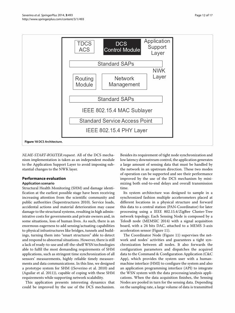
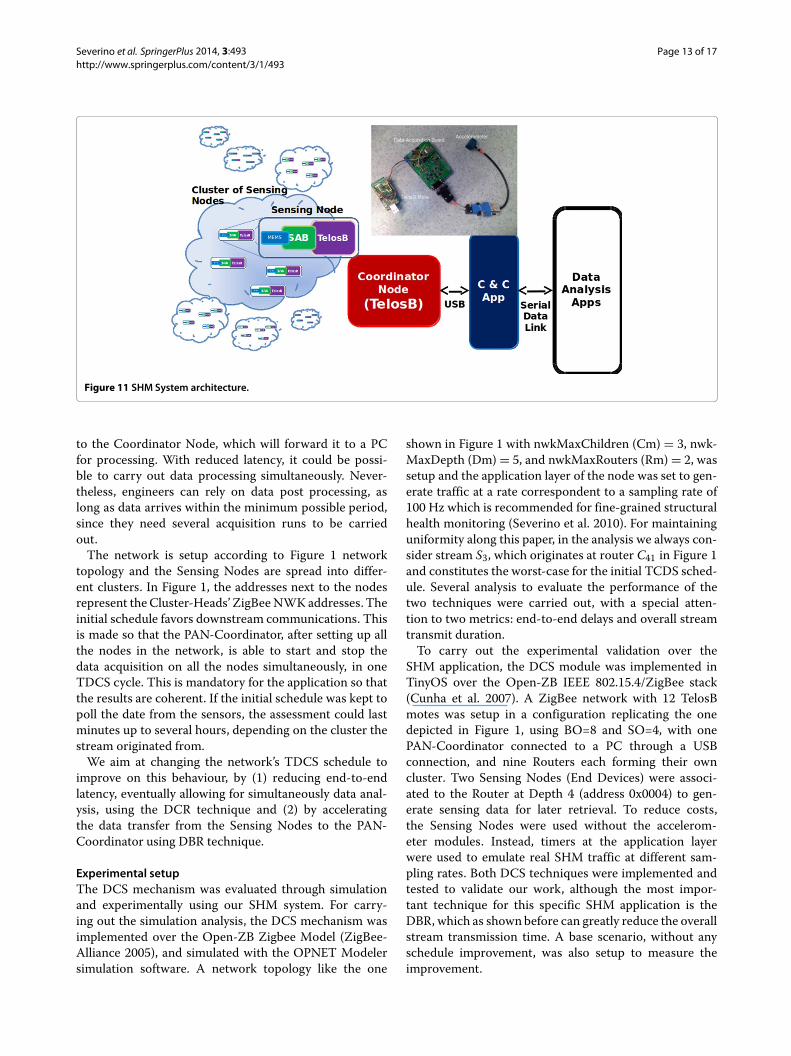
synchronized fashion multiple accelerometers placed atdifferent locations in a physical structure and forwardthis data to a central station (PAN-Coordinator) for laterprocessing using a IEEE 802.15.4/ZigBee Cluster-Treenetwork topology. Each Sensing Node is composed by aTelosB node (MEMSIC 2014) with a signal acquisitionboard, with a 24 bits DAC, attached to a MEMS 3-axisacceleration sensor (Figure 11).The Coordinator Node (Figure 11) supervises the net-

work and nodes’ activities and guarantees a tight syn-chronization between all nodes. It also forwards theconfiguration parameters and dispatches the acquireddata to the Command & Configuration Application (C&CApp), which provides the system user with a human-machine interface (HMI) to configure the system and alsoan application programming interface (API) to integratethe WSN system with the data processing/analysis appli-cations. When the data acquisition finishes, the SensingNodes are pooled in turn for the sensing data. Dependingon the sampling rate, a large volume of data is transmitted

Severino et al. SpringerPlus 2014, 3:493 Page 13 of 17http://www.springerplus.com/content/3/1/493

Figure 11 SHM System architecture.

to the Coordinator Node, which will forward it to a PCfor processing. With reduced latency, it could be possi-ble to carry out data processing simultaneously. Never-theless, engineers can rely on data post processing, aslong as data arrives within the minimum possible period,since they need several acquisition runs to be carriedout.The network is setup according to Figure 1 network

topology and the Sensing Nodes are spread into differ-ent clusters. In Figure 1, the addresses next to the nodesrepresent the Cluster-Heads’ ZigBeeNWK addresses. Theinitial schedule favors downstream communications. Thisis made so that the PAN-Coordinator, after setting up allthe nodes in the network, is able to start and stop thedata acquisition on all the nodes simultaneously, in oneTDCS cycle. This is mandatory for the application so thatthe results are coherent. If the initial schedule was kept topoll the date from the sensors, the assessment could lastminutes up to several hours, depending on the cluster thestream originated from.We aim at changing the network’s TDCS schedule to

improve on this behaviour, by (1) reducing end-to-endlatency, eventually allowing for simultaneously data anal-ysis, using the DCR technique and (2) by acceleratingthe data transfer from the Sensing Nodes to the PAN-Coordinator using DBR technique.

Experimental setupThe DCS mechanism was evaluated through simulationand experimentally using our SHM system. For carry-ing out the simulation analysis, the DCS mechanism wasimplemented over the Open-ZB Zigbee Model (ZigBee-Alliance 2005), and simulated with the OPNET Modelersimulation software. A network topology like the one

shown in Figure 1 with nwkMaxChildren (Cm) = 3, nwk-MaxDepth (Dm)= 5, and nwkMaxRouters (Rm)= 2, wassetup and the application layer of the node was set to gen-erate traffic at a rate correspondent to a sampling rate of100 Hz which is recommended for fine-grained structuralhealth monitoring (Severino et al. 2010). For maintaininguniformity along this paper, in the analysis we always con-sider stream S3, which originates at router C41 in Figure 1and constitutes the worst-case for the initial TCDS sched-ule. Several analysis to evaluate the performance of thetwo techniques were carried out, with a special atten-tion to two metrics: end-to-end delays and overall streamtransmit duration.To carry out the experimental validation over the

SHM application, the DCS module was implemented inTinyOS over the Open-ZB IEEE 802.15.4/ZigBee stack(Cunha et al. 2007). A ZigBee network with 12 TelosBmotes was setup in a configuration replicating the onedepicted in Figure 1, using BO=8 and SO=4, with onePAN-Coordinator connected to a PC through a USBconnection, and nine Routers each forming their owncluster. Two Sensing Nodes (End Devices) were associ-ated to the Router at Depth 4 (address 0x0004) to gen-erate sensing data for later retrieval. To reduce costs,the Sensing Nodes were used without the accelerom-eter modules. Instead, timers at the application layerwere used to emulate real SHM traffic at different sam-pling rates. Both DCS techniques were implemented andtested to validate our work, although the most impor-tant technique for this specific SHM application is theDBR, which as shownbefore can greatly reduce the overallstream transmission time. A base scenario, without anyschedule improvement, was also setup to measure theimprovement.

Severino et al. SpringerPlus 2014, 3:493 Page 14 of 17http://www.springerplus.com/content/3/1/493

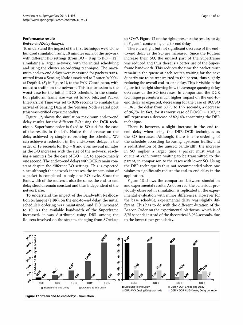
Performance resultsEnd-to-endDelay AnalysisTo understand the impact of the first techniquewe did onehundred simulation runs, 10 minutes each, of the networkwith different BO settings (from BO = 8 up to BO = 12),simulating a larger network, with the initial schedulingand using the cluster re-ordering technique. The maxi-mum end-to-end delays were measured for packets trans-mitted from a Sensing Node associated to Router 0x0004,at Depth 4, (S3 in Figure 1), to the PAN-Coordinator, withno extra traffic on the network. This transmission is theworst-case for the initial TDCS schedule. In the simula-tion platform, frame size was set to 800 bits, and PacketInter-arrival Time was set to 0,06 seconds to emulate thearrival of Sensing Data at the Sensing Node’s serial port(this was verified experimentally).Figure 12, shows the simulation maximum end-to-end

delay results for the different BO using the DCR tech-nique. Superframe order is fixed to SO = 4 for the caseof the results in the left. Notice the decrease on thedelay achieved by simply re-ordering the schedule. Wecan achieve a reduction in the end-to-end delays in theorder of 13 seconds for BO = 8 and even several minutesas the BO increases with the size of the network, reach-ing 4 minutes for the case of BO = 12, to approximatelyone second. The end-to-end delays withDCR remain con-stant despite the different BO settings. This is expectedsince although the network increases, the transmission ofa packet is completed in only one BO cycle. Since theBandwidth of the routers is also the same, the end-to-enddelay should remain constant and thus independent of thenetwork size.To understand the impact of the Bandwidth Realloca-

tion technique (DBR), on the end-to-end delay, the initialschedule’s ordering was maintained, and BO increasedto 10. As the available bandwidth of the Superframeincreased, it was distributed using DBR among theRouters involved on the stream, changing from SO=4 up

to SO=7. Figure 12 on the right, presents the results for S3in Figure 1 concerning end-to-end delay.There is a slight but not significant decrease of the end-

to-end delay as the SO are increased. Since the Routersincrease their SO, the unused part of the Superframewas reduced and thus there is a better use of the Super-frame bandwidth. This reduces the time the packet mustremain in the queue at each router, waiting for the nextSuperframe to be transmitted to the parent, thus slightlyreducing the overall end-to-end delay. This is visible in thefigure in the right showing how the average queuing delaydecreases as the SO increases. In comparison, the DCRtechnique presents a much higher impact on the end-to-end delay as expected, decreasing for the case of BO/SO= 10/5, the delay from 60,95 to 1,97 seconds, a decreaseof 96,7%. In fact, for its worst case of BO/SO = 10/7, itstill represents a decrease of 82,14% concerning the DBRtechnique.There is however, a slight increase in the end-to-

end delay when using the DBR+DCR techniques asthe SO increases. Although, there is a re-ordering ofthe schedule according favouring upstream traffic, anda redistribution of the unused bandwidth, the increasein SO implies a larger time a packet must wait inqueue at each router, waiting to be transmitted to theparent, in comparison to the cases with lower SO. Usingthe DBR technique is thus not recommended when onewishes to significantly reduce the end-to-end delay in theapplication.Figure 13 shows the comparison between simulation

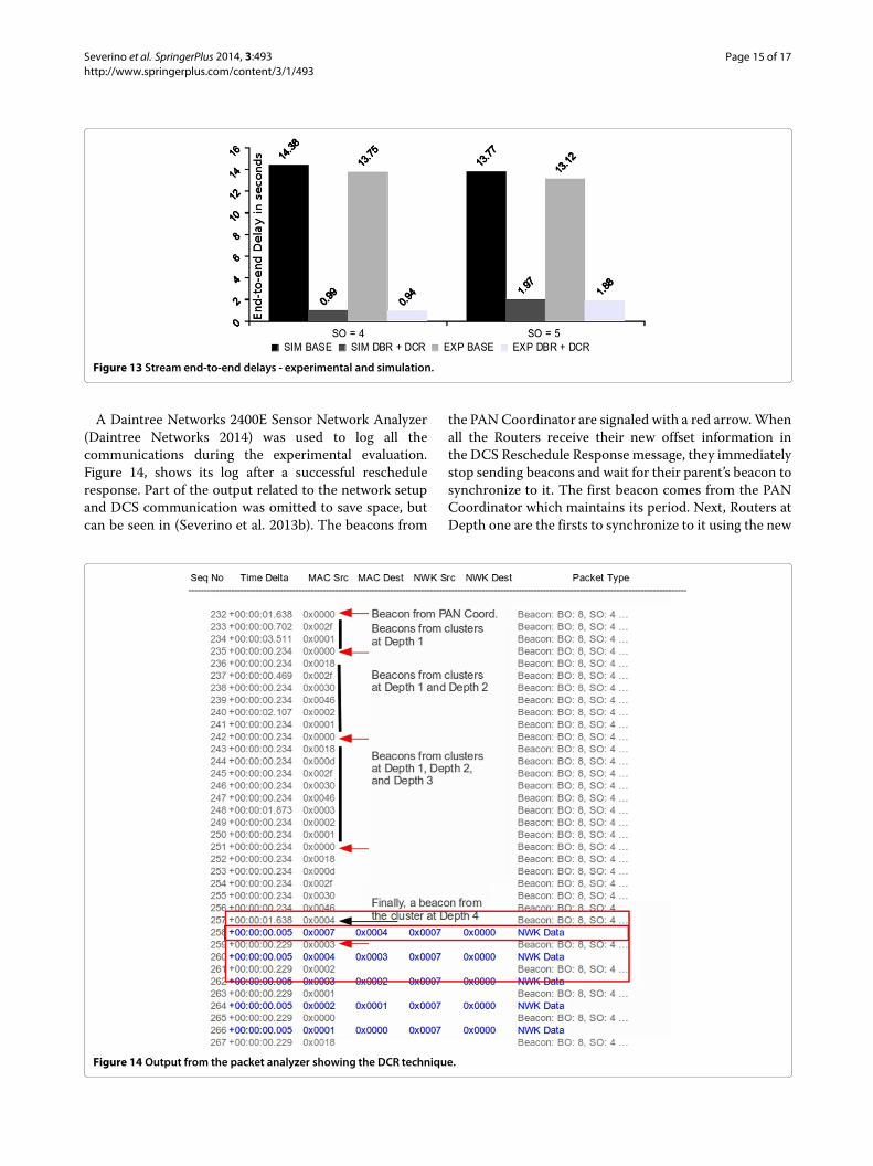
and experimental results. As observed, the behaviour pre-viously observed in simulation is replicated in the exper-imental evaluation with minor differences. However forthe base schedule, experimental delay was slightly dif-ferent. This has to do with the different duration of theBeacon Order on the experimental platforms, which is of3,75 seconds instead of the theoretical 3,932 seconds, dueto the lower timer granularity.

Figure 12 Stream end-to-end delays - simulation.

Severino et al. SpringerPlus 2014, 3:493 Page 15 of 17http://www.springerplus.com/content/3/1/493

Figure 13 Stream end-to-end delays - experimental and simulation.

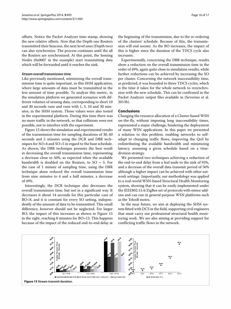
A Daintree Networks 2400E Sensor Network Analyzer(Daintree Networks 2014) was used to log all thecommunications during the experimental evaluation.Figure 14, shows its log after a successful rescheduleresponse. Part of the output related to the network setupand DCS communication was omitted to save space, butcan be seen in (Severino et al. 2013b). The beacons from

the PANCoordinator are signaled with a red arrow.Whenall the Routers receive their new offset information inthe DCS Reschedule Response message, they immediatelystop sending beacons and wait for their parent’s beacon tosynchronize to it. The first beacon comes from the PANCoordinator which maintains its period. Next, Routers atDepth one are the firsts to synchronize to it using the new

Figure 14 Output from the packet analyzer showing the DCR technique.

Severino et al. SpringerPlus 2014, 3:493 Page 16 of 17http://www.springerplus.com/content/3/1/493

offsets. Notice the Packet Analyzer time stamp, showingthe new relative offsets. Now that the Depth one Routerstransmitted their beacons, the next level ones (Depth two)can also synchronize. The process continues until the allthe Routers are synchronized. At this point, the SensingNodes (0x0007 in the example) start transmitting datawhich will be forwarded until it reaches the sink.

Streamoverall transmission timeLike previously mentioned, minimizing the overall trans-mission time is quite important, in this SHM application,where large amounts of data must be transmitted in theless amount of time possible. To analyze this metric, inthe simulation platform we generated scenarios with dif-ferent volumes of sensing data, corresponding to short 10and 30 seconds runs and runs with 1, 5, 10 and 30 min-utes, in the SHM system. Those values were also testedin the experimental platform. During this time there wasno more traffic in the network, so that collisions were notpossible, not to interfere with the experiment.Figure 15 shows the simulation and experimental results

of the transmission time for sampling durations of 30, 60seconds and 5 minutes using the DCR and DBR tech-niques for SO=4 and SO=5 in regard to the base schedule.As shown, the DBR technique presents the best resultin decreasing the overall transmission time, representinga decrease close to 50%, as expected when the availablebandwidth is doubled on the Routers, to SO = 5. Forthe case of 1 minute of sampling time, using the DBRtechnique alone reduced the overall transmission timefrom nine minutes to 4 and a half minutes, a decreaseof 49%.Interestingly, the DCR technique also decreases the

overall transmission time, but not in a significant way. Itdecreases it about 14 seconds for this particular case ofBO=8, and it is constant for every SO setting, indepen-dently of the amount of data to be transmitted. This smalldifference, however should not be neglected. For largerBO, the impact of this increases as shown in Figure 15in the right, reaching 8 minutes for BO=13. This happensbecause of the impact of the reduced end-to-end delay at

the beginning of the transmission, due to the re-orderingof the clusters’ schedule. Because of this, the transmis-sion will end sooner. As the BO increases, the impact ofthis is higher since the duration of the TDCS cycle alsoincreases.Experimentally, concerning the DBR technique, results

show a reduction on the overall transmission time in theorder of 49%, again quite close to simulation results, whilefurther reductions can be achieved by increasing the SOper cluster. Concerning the network inaccessibility time,as predicted, it was bounded to three TDCS cycles, whichis the time it takes for the whole network to resynchro-nize with the new schedule. This can be confirmed in thePacket Analyzer output files available in (Severino et al.2013b).

ConclusionsChanging the resource allocation of a Cluster-basedWSNon-the-fly, without imposing long inaccessibility times,represented a major challenge, hindering the deploymentof many WSN applications. In this paper we presenteda solution to this problem, enabling networks to self-adapt to changing traffic flows, improving the QoS byredistributing the available bandwidth and minimizinglatency, assuming a given schedule based on a time-division strategy.We presented two techniques achieving a reduction of

the end-to-end delay from a leaf node to the sink of 93%,and a decrease of the overall data transmit period of 50%although a higher impact can be achieved with other net-work settings. Importantly, our methodology was appliedto a real-worldWSN-based Structural Health Monitoringsystem, showing that it can be easily implemented underthe IEEE802.15.4/ZigBee set of protocols with minor add-ons and can run in general purpose WSN platforms suchas the TelosB motes.In the near future, we aim at deploying the SHM sys-

tem fitted withDCS in the field, supporting civil engineersthat must carry out professional structural health moni-toring work. We are also aiming at providing support forconflicting traffic flows in the network.

Figure 15 Stream transmit duration.

Severino et al. SpringerPlus 2014, 3:493 Page 17 of 17http://www.springerplus.com/content/3/1/493

Competing interestsThe authors declare that they have no competing interests.

Authors’ contributionsRS proposed, designed and carried out the evaluation of the DCS mechanism.Dr. NP and Dr. ET participated in the design of the proposed mechanism anddrafting of the manuscript. All authors read and approved the final version ofthe manuscript.

AcknowledgementsThis work was supported by PT Funds through FCT (Portuguese Foundationfor Science and Technology), by ESF (European Social Fund) through POPH(Portuguese Human Potential Operational Program), under grantSFRH/BD/71573/2010. It was also supported by ERDF (European RegionalDevelopment Fund) through COMPETE (Operational Programme ’ThematicFactors of Competitiveness’), within projects FCOMP-01-0124-FEDER-014922(MASQOTS), FCOMP-01-0124-FEDER-012988 (SENODS),FCOMP-01-0124-FEDER-020312 (SMARTSKIN).

Received: 04 July 2014 Accepted: 12 August 2014Published: 31 August 2014

ReferencesAbdelzaher TF, Prabh S, Kiran R (2004) On real-time capacity limits of multihop

wireless sensor networks. In: Proceedings of the 25th Real-Time SystemsSymposium, (RTSS 2004). IEEE Computer Society, Washington, DC, USA,pp 359–370

Aguilar R, Ramos L, Lourenço P, Severino R, Gomes R, Gandra P, Alves M,Tovar E (2011) Prototype wsn platform for performing dynamic monitoringof civil engineering structures. In: Sensors, Instrumentation and SpecialTopics, Conference Proceedings of the Society for Experimental MechanicsSeries 2011, vol 6. Springer, New York, NY, USA, pp 81–89

Burda R, Wietfeld C (2007) A distributed and autonomous beacon schedulingalgorithm for ieee 802.15.4/zigbee networks. In: Proceedings of IEEEInternatonal Conference On Mobile Adhoc and Sensor Systems(MASS 2007). IEEE Computer Society, Washington, DC, USA, pp 1–6

Choi H, Wang J, Hughes E (2009) Scheduling for information gathering onsensor network. Wireless Netw 15(1):127–140

Cunha A, Koubaa A, Severino R, Alves M (2007) Open-zb: an open-sourceimplementation of the ieee 802.15.4/zigbee protocol stack on tinyos. In:Proceedings of the 4th IEEE International Conference in Mobile Adhoc andSensor Systems (MASS 2007). IEEE Computer Society, Washington, DC,USA, pp 1–12

Cunha A, Severino R, Pereira N, Koubâa A, Alves M (2008) Zigbee over tinyos:implementation and experimental challenges. In: Proceedings of the 8thPortuguese Conference on Automatic Control (CONTROLO’2008), Vila Real,Portugal, pp 21–23

Dan L, Zhihong Q, Xu Z, Yue L (2010) Research on tree routing improvementalgorithm in zigbee network. In: Proceedings of the 2nd InternationalConference in Multimedia and Information Technology (MMIT 2010), vol.1. IEEE Computer Society, Washington, DC, USA, pp 89–92

Di Francesco M, Pinotti CM, Das SK (2012) Interference-free scheduling withbounded delay in cluster-tree wireless sensor networks. In: Proceedings ofthe 15th ACM International Conference on Modeling, Analysis andSimulation of Wireless and Mobile Systems (MSWiM ’12). ACM, New York,NY, USA, pp 99–106

Gandham S, Zhang Y, Huang Q (2008) Distributed time-optimal scheduling forconvergecast in wireless sensor networks. Comput Netw 52(3):610–629

Gibson J, Xie GG, Xiao Y (2007) Performance limits of fair-access in sensornetworks with linear and selected grid topologies. In: Proceedings ofGlobal Telecommunications Conference (GLOBECOM ’07). IEEE ComputerSociety, Washington, DC, USA, pp 688–693

Hanzalek Z, Jurcik P (2010) Energy efficient scheduling for cluster-tree wirelesssensor networks with time-bounded data flows: Application to ieee802.15.4/zigbee. IEEE Trans Ind Inform 6(3):438–450

Huang Y-K, Pang A-C, Hsiu P-C, Zhuang W, Liu P (2012) Distributed throughputoptimization for zigbee cluster-tree networks. IEEE Trans ParallelDistributed Syst 23(3):513–520

Incel OD, Ghosh A, Krishnamachari B, Chintalapudi K (2012) Fast datacollection in tree-based wireless sensor networks. IEEE Trans MobileComput 11(1):86–99

IEEE Standard for Information technology (2006) Local and metropolitan areanetworks– Specific requirements– Part 15.4: Wireless Medium AccessControl (MAC) and Physical Layer (PHY) Specifications for Low RateWireless Personal Area Networks (WPANs):1–320

Jurcik P, Koubâa A, Severino R, Alves M, Tovar E (2010) Dimensioning andworst-case analysis of cluster-tree sensor networks. ACM Trans SensorNetw 7(2):Article:14

Kim T, Kim D, Park N, Yoo S-E, Lopez TS (2007) Shortcut tree routing in zigbeenetworks. In: Proceedings of the 2nd International Symposium on WirelessPervasive Computing, (ISWPC’07). IEEE Computer Society, Washington, DC,USA, pp 5–7

Koubaa A, Cunha A, Alves M (2007) A time division beacon schedulingmechanism for ieee 802.15.4/zigbee cluster-tree wireless sensor networks.In: Proceedings of the 19th Euromicro Conference on Real-Time Systems,2007. (ECRTS ’07). IEEE Computer Society, Washington, DC, USA,pp 125–135

Lai N-L, King C-T, Lin C-H (2008) On maximizing the throughput ofconvergecast in wireless sensor networks. In: Advances in Grid andPervasive Computing, vol. 5036. Lecture Notes in Computer Science.Springer, Berlin, Heidelberg, pp 396–408

Muthukumaran P, de Paz R, Spinar R, Pesch D (2010) Meshmac: Enabling meshnetworking over ieee 802.15. 4 through distributed beacon scheduling. In:Ad Hoc Networks, Lecture Notes of the Institute for Computer Sciences,Social Informatics and Telecommunications Engineering. vol. 28. Springer,Berlin, Heidelberg, pp 561–575

MEMSIC WSN Products, TelosB, Online (2014). http://www.memsic.com/wireless-sensor-networks/

Open-ZB Website, Online (2014). http://www.open-zb.netPan M-S, Tseng Y-C (2008) Quick convergecast in zigbee beacon-enabled

tree-based wireless sensor networks. Comput Commun 31(5):999–1011Prabh KS, Abdelzaher TF (2007) On scheduling and real-time capacity of

hexagonal wireless sensor networks. In: Proceedings of the 19th EuromicroConference on Real-Time Systems. ECRTS ’07. IEEE Computer Society,Washington, DC, USA, pp 136–145

Raman B, Chebrolu K (2008) Censor networks: a critique of “sensor networks”from a systems perspective. SIGCOMM Comput Commun Rev 38(3):75–78

Severino R, Gomes R, Alves M, Sousa P, Tovar E, Ramos LF, Aguilar R, LourençoPB (2010) A wireless sensor network platform for structural healthmonitoring: enabling accurate and synchronized measurements throughcots+custom-based design. In: Proceedings of the 5th Conference onManagement and Control of Production Logistics (2010). IFAC,International Federation of Automation and Control, Coimbra, Portugal,pp 375–382

Severino R, Pereira N, Tovar E (2013a) Dynamic cluster scheduling forcluster-tree WSNs. In: Proceedings of the 9th workshop on softwaretechnologies for future embedded and ubiquitous systems (SEUS 2013).IEEE Computer Society, Washington, DC, USA

Severino R, Pereira N, Tovar E (2013b) Dynamic cluster scheduling forcluster-tree wsns. Technical report, CISTER-TR-130205. http://www.cister.isep.ipp.pt/docs/

Stankovic JA, Lee I, Mok A, Rajkumar R (2005) Opportunities and obligations forphysical computing systems. Computer 38(11):23–31

Sensor Network Analyzer(SNA), Online (2014). http://www.daintree.netThe Economist (2010) In: Technology Quarterly: Q4, Inside Story:

Superstructures. Online: http://www.economist.com/node/17647603TinyOS Operating System Website, Online (2014). http://www.tinyos.netToscano E, Lo Bello L (2009) A multichannel approach to avoid beacon

collisions in ieee 802.15.4 cluster-tree industrial networks. In: Proceedingsof the 14th IEEE Conference on Emerging Technologies FactoryAutomation (ETFA 2009). IEEE Press, Piscataway, NJ, USA, pp 1242–1250

Yeh L-W, Pan M-S, Tseng Y-C (2008) Two-way beacon scheduling in zigbeetree-based wireless sensor networks. In: Proceedings of the 8th IEEEInternational Conference on Sensor Networks, Ubiquitous and TrustworthyComputing, (SUTC 2008). IEEE Computer Society, Washington, DC, USA,pp 130–137

Zigbee-Alliance (2005) ZigBee specification: Technical Report Document053474r06, Version 1.0. ZigBee Alliance. San Ramon, CA, USA

doi:10.1186/2193-1801-3-493Cite this article as: Severino et al.: Dynamic cluster scheduling forcluster-tree WSNs. SpringerPlus 2014 3:493.