1

TAN: a Distributed Algorithm for Dynamic TaskAssignment in WSNs

Virginia Pilloni∗, Pirabakaran Navaratnam†, Serdar Vural†, Luigi Atzori∗, Rahim Tafazolli†∗DIEE, University of Cagliari, Italy virginia.pilloni,l.atzori@diee.unica.it

†CCSR, University of Surrey, Guildford, UK p.navaratnam,s.vural,r.tafazolli@surrey.ac.uk

F

Abstract—We consider the scenario of Wireless Sensor Networkswhere a given application has to be deployed and each application taskhas to be assigned to each node in the best possible way. Approacheswhere decisions on task execution are taken by a single central nodecan avoid the exchange of data packets between task execution nodesbut cannot adapt to dynamic network conditions, and suffer from com-putational complexity. To address this issue, in this paper we proposean adaptive and decentralised Task Allocation Negotiation algorithm(TAN) for cluster network topologies. It is based on non-cooperativegame theory, where neighbouring nodes engage in negotiations tomaximize their own utility functions to agree on which of them shouldexecute single application tasks. Performance are evaluated in a cityscenario, where the urban streets are equipped with different sensorsand the application target is the detection of the fastest way to reacha destination, and in random WSN scenarios. Comparisons are madewith three other algorithms: (i) baseline setting with no task assignmentto multiple nodes, (ii) centralised task assignment lifetime optimisation,and (iii) a dynamic distributed algorithm, DLMA. It results that TANoutperforms these algorithms in terms of application completion timeand average energy consumption.

Index Terms—Wireless Sensor Networks, task assignment, game the-ory.

1 INTRODUCTION

The progress in Wireless Sensor Network (WSN) technol-ogy, both in terms of processing capability and energyconsumption reduction, has evolved WSNs into complexsystems that can gather information about the monitoredenvironment and make prompt and intelligent decisions.These developments have contributed to the efforts onintegrating sensor devices in Future Internet (FI) ar-chitectures [1], which enables effective interfacing withother technologies. In doing so, a horizontal ambientintelligent infrastructure is made possible, wherein thesensing, computing, and communicating tasks can becompleted using programmable middleware that en-ables quick deployment of different applications andservices.

Copyright c© 2013 IEEE. Personal use of this material is permitted. However,permission to use this material for any other purposes must be obtained fromthe IEEE by sending a request to pubs-permissions@ieee.orgThis work has been partially funded by the project Artemis JU Demanes, De-sign, Monitoring and Operation of Adaptive Networked Embedded Systems,grant agreement no. 295372.

One of the major issues with WSNs is maximisationof network lifetime, due to the fact that sensors aremainly battery powered. Many efforts have been madeso as to extend network lifetime, one of which is thedevelopment of algorithms that effectively assign exe-cution tasks to network nodes. One method to performtask assignment is the use of a central controller thatdivides large application programs into smaller andeasily executable tasks and then distributes these tasksto nodes. Task allocation solutions that consider a centralcontroller are called centralised solutions. For instance,in [2] a centralised solution for the maximization of theWSN lifetime is proposed. In [3][4][5], centralised algo-rithms for both reducing network energy consumptionand application execution time are proposed. However,these centralised algorithms suffer from computationalcomplexity, especially for WSNs with a large numberof nodes. Furthermore, centralised algorithms have tofrequently collect updates from nodes in order to adaptto network dynamics, which is difficult to achieve andincurs large control packet overhead.

Due to the drawbacks of centralised solutions, dis-tributed solutions are recently proposed to perform taskallocation in WSNs. For instance, in [6] a communica-tion scheme based on gossiping is used, while in [7]a particle swarm optimization algorithm is adopted.These distributed algorithms reduce the problem com-plexity, as only local areas are considered rather than thewhole network. The communication overhead causedby packet exchanges between network nodes and thecentral controller is also avoided. Nevertheless, noneof them take into account the execution time of theapplication assigned to the network. This could lead toan inconvenient task assignment strategy, which mayentail that the application deadline is reached before theapplication is executed.

In this paper, a new distributed algorithm for theallocation of application tasks among WSN nodes isproposed, which is named Task Allocation Negotiation(TAN). This algorithm aims to reduce application ex-ecution time as much as possible, with minimal net-work energy consumption while inducing less compu-

2

tational complexity than existing algorithms have. Themajor contribution is the adoption of the rules of non-cooperative game theory [8]. Sensor nodes negotiateamong each other to set the application configuration.In doing so, each node aims at maximising a nodeutility function under the constraints set by neighbouringsensors. We then prove that the scenario under consid-eration is a potential game [9], which means that everyimprovement of the nodes’ utility functions correspondsto the same improvement in the utility perceived by thewhole network, which implies that the problem has aunique outcome that is reachable in finite time.

The obtained solution reduces the average node en-ergy consumption rate (and hence contributes to net-work lifetime extension) and simultaneously meets theapplication completion time requirements. Simulationresults show significant performance improvements inboth average node energy consumption and applicationcompletion time in a illustrative smart city scenario,where we assume that urban streets are equipped withdifferent sensors and the application target is the de-tection of the fastest way to reach a destination onthe basis of the current average travelling times. Sim-ulations are evaluated with respect to three settings:(i) the case where the whole application is carried outby a single sensor node, (ii) the centralized task assign-ment approach presented in [2], and (iii) the distributedtask assignment approach presented in [6]. Furthermore,TAN is tested for random WSN scenarios. Noticeablegains are obtained for networks with high node densityand highly populated clusters, especially when TAN isapplied to complex applications.

This paper is organized as follows. Section 2 presentsthe related works, Section 3 introduces the problemand briefly describes the proposed approach, Section4 describes the task assignment model, and Section 5describes the algorithm. Finally, Sections 6 and 7 presentthe simulation results and conclusions.

2 RELATED WORK

Since nodes in WSNs are battery powered, a great dealof effort has been made by researchers to find effec-tive strategies that increase network lifetime. Differentapproaches have been proposed to this end. Some ex-amples are: convenient deployment of sensors [10], useof efficient routing techniques [11], and use of static ormobile relay nodes that help balance network energyconsumption among nodes [12]. However, due to theadvances in microchip technology, which provide addi-tional capabilities to sensors, more advanced methodsthat extend network lifetime are now possible, besidesthese traditional techniques that either modify networktopology or provide an energy-efficient routing protocol.Therefore, not only is network lifetime optimisation notonly is centred on reduction of packet transmissionpower, but it also involves convenient data processingthat reduces the amount of data delivered to data sinks.

This is the principle behind node clustering protocols,such as LEACH [13] and EC [14], in which clusterhead nodes aggregate data and reduce transmitted datavolume, which in turn reduces the overall transmissionenergy consumption of the network.

A step forward in extending network lifetime is to con-sider not only data aggregation to reduce data volume,but also any possible data processing tasks based onnetwork topology, battery power, and node processingcapabilities. However, existing methods have limitedscope in studying lifetime extension with regards toapplication data processing. For instance, in [15], max-imization of cluster lifetimes is studied. However, thisapproach considers only communication tasks, but notthe tasks generated by applications and assigned tothe network for execution. Furthermore, it only focuseson homogeneous networks, which are not common inreal scenarios. In contrast, [16] considers execution ofapplication tasks, and provides an adaptive task alloca-tion algorithm that aims at reducing the overall energyconsumption by balancing residual node energy levels.However, this mechanism requires exchange of someadditional messages among all the nodes in the network,which considerably increases packet overhead.

Some other studies in [3][4][5], improve network life-time while reducing task execution time. However, thealgorithms in these works are centralised, and thereforesuffer from computational complexity, as well as largecontrol packet overhead due to frequent updates col-lected from nodes in order to adapt to network dynam-ics.

To overcome the issues encountered by centralised so-lutions, the authors in [6] propose an overlaying frame-work that determines the distribution of tasks among thenodes in a WSN by means of a distributed optimizationalgorithm, based on a gossip communication scheme,aimed at maximizing network lifetime. A similar ap-proach is studied in [7], where a distributed algorithm isproposed based on particle swarm optimization. How-ever, the major drawback of these studies is that theydo not take into account the deadline of the applicationsassigned to the network.

Network lifetime improvement through distributedtask assignment is a crucial issue also in other fields.In [17], task assignment is considered from the robots’point of view. In this works, the authors propose twoauction clearing algorithms to assign the best task as-signment pattern to robots in a distributed way, in sucha way that the overall energy consumption is reduced.Three task assignment protocols that tackle the issue ofallocating destroy targets scenario tasks to UnmannedAerial Vehicles (UAVs) are presented in [18]. The dis-tributed algorithms proposed in this work are based onteam theory and game theory. The last two works are abit far from the scenarios considered in this paper, whichare composed of a number of agents considerably higher.Nevertheless, they have in common the characteristicthat high communication costs make centralised task

3

allocation algorithms unsuitable due to their cost.

3 PROBLEM FORMULATIONThe reference scenario considered in this paper is thatof a hierarchical heterogeneous WSN. The WSN is hier-archically organised into clusters, with sensor nodes ascluster members, and cluster heads. The heterogeneityreflects the fact that, in most real scenarios, nodes withdifferent characteristic parameters are used. The WSNunder examination needs to run a required application,which can be divided into smaller tasks that can beassigned to network nodes to be executed. Due to theheterogeneous node characteristics, some nodes can per-form the same task faster than others, and even spendless energy. The objective of the proposed algorithm,TAN, is to assign the tasks to suitable nodes, such thatthe processing time of the application is as short aspossible and the network lifetime is as long as possible.TAN includes negotiations among nodes to determinetask assignments. Whenever a node receives some data(along with the information on which particular taskshave to be performed on the data) it decides whetherit should perform some tasks or not, depending on thepotential contribution to the network in terms of fasterprocessing time and longer lifetime.

3.1 Network ModelThe network is modelled as a Directed Acyclic Graph(DAG) GX = (X,EX), where the vertices representthe nodes X = 1, . . . , i, . . . , N, while the links aredescribed by the set of edges EX = (eij), where eachedge represents a connection from node i to node j.The network is organised into clusters. Each cluster iscontrolled by a single cluster head (CH) which collectssensory data from nodes in its cluster. There is a singlehop between a sensor node and its corresponding CH. Atthe top of the hierarchy is a gateway (GW) node, whichcollects data received from the CHs. Sensors transmittheir data to the CHs, which then deliver the collecteddata to the gateway through a path of CHs. Rout-ing paths over the CHs is determined by conventionalrouting protocols [19], such as Self-Organizing Protocol,Location-Based Routing Protocol, etc. In this paper, Hi-erarchical Power-Aware Routing protocol is used [20],due to the fact that it is based on a trade-off betweenminimizing power consumption and maximizing theminimal residual power of the network.

Negotiations are performed among neighbour nodes;multihop negotiations do not take place, and this signif-icantly reduces the number of message exchanges. Nocommunication is allowed between sensors belonging todifferent clusters. This means that, given two nodes iand j, eij ∈ EX if and only if i and j are in the samecluster. Such an architecture helps reduce the overheadcaused by the negotiations. Figure 1 shows the referencearchitecture of the network under examination. In thisFigure, SNi and CHj are communicating with theirneighbours.

Fig. 1: Architecture of the network. Solid lines representconnections formed by the routing protocol; dashed linesrepresent connections between negotiation nodes.

3.2 Task Model

We consider a single large application assigned to thenetwork for execution, which is decomposed into a setof tasks. This application can be described as a DAG oftasks GT = (T,ET ), where T = 1, . . . , λ, . . .Λ is the setof tasks, and ET = (evw) is the set of edges, with eachedge evw representing a unidirectional data transfer fromtask v to task w. An example of the task DAG is depictedin Figure 2. The gateway initially sends the applicationgraph GT to nodes, so that each node learns the relationsand dependencies between the tasks.

Fig. 2: Example of a task DAG.

A binary vector s(i) = [s(i, λ)], for λ ∈ T , can beassigned to each node i in the network, where s(i, λ)is a boolean value representing the current state ofnode i corresponding to task λ, i.e. s(i, λ) = 1 whennode i is performing task λ. The vector s(i) is calledthe task assignment strategy of node i. The state s(i, λ)can only be set to 1 if and only if all its predecessortasks have been assigned to a node, i.e. s(i, λ) = 1 ifs(j, l) = 1, ∀l ∈ Tin(λ), where Tin(λ) are the ingresstasks for task λ. With reference to Figure 2, Tin(T1) =Tin(T2) = Tin(T3) = Tin(T5) = , hence they are source

4

tasks, Tin(T4) = T1, T2, T3, and Tin(T6) = T4, T5.Since not every node may be able to perform each and

every task, a binary vector d(i) = (d(i, λ)) is defined,where d(i, λ) = 1 if node i is able to perform task λ.Note that s(i, λ) = 1 is possible only if d(i, λ) = 1, whichmeans that d(i, λ) ≥ s(i, λ).

During the execution of the proposed algorithm, twosets of tasks are formed: the set of tasks Tprev =1, . . . , h, . . . ,H that have been already assigned tonodes and the set Tnext = 1, . . . , k, . . . ,K of those tasksthat are yet to be assigned. This means that, for eachtask h ∈ Tprev , there is a node i for which its state s(i, h)is equal to 1. We assume that source tasks are alreadyassigned to the nodes by the gateway according to theoutput required by the application. For example, if theapplication requires the temperature measurement for acertain area, source tasks correspond to the temperaturesensing for that area. In this case, the gateway assignsthese source tasks to the sensor nodes (SNs) that arelocated in that area. Hence, initially, the set Tprev isonly populated with source tasks, i.e. with reference toFigure 2, Tprev = T1, T2, T3, T5 and Tnext = T4, T6.

4 THE TASK ASSIGNMENT MODEL

The aim of the optimization problem is to finding thetrade-off that best fits the requirements of both mini-mizing the application completion time and maximizingthe network lifetime. However, this is an NP-hard prob-lem [2][3], which could be exceedingly time and energyconsuming. For this reason, in this section, we use a non-cooperative game model [21] for the task allocation prob-lem in WSNs. Neighbouring nodes negotiate in order foreach node i to choose a task assignment strategy s(i) thatmaximizes its own utility function.

4.1 Definitions

A non-cooperative game is defined by the tuple Γ =〈X, s(i), uii∈X〉, where a utility function ui is assignedto node i ∈ X for the given strategy vector s(i). The goalof each node is to maximize its own utility in a rationalway. Therefore, a strategy s∗(i) is preferred to a strategys(i) if and only if ui(s∗(i)) > ui(s(i)). For simplicity, wedenote S =

⋃i∈X s(i) to refer to the strategy of all the

nodes in the network.In the following, we consider each node i as char-

acterised by five parameters, which are described inTable 1.

4.2 Task Utility Function

The TAN algorithm decides which particular nodeshould execute a given task k by maximizing a task utilityfunction over the set Tnext of unassigned nodes, given by:

uk(S) = maxi∈X

[Ωt(i, k) +

α

NF (k)· Ωτ (i, k,S)

]· s(i, k)

,

(1)

TABLE 1: Node parameters

Parameter Description

tinstr(i)Time needed by node i to perform asingle instruction

eins(i)Energy spent by node i to perform asingle instruction

etx(i) = (etx(i, j))Each element etx(i, j) of this vector isthe energy spent per bit to send datafrom node i to an adjacent node j

erx(i) Per bit reception energy at node ieres(i) Residual energy of node i

where Ωt(i, k) is the task completion time component oftask k when it is performed by node i, Ωτ (i, k,S) isthe network lifetime component when task k is performedby node i according to the strategy S, NF (k) is anormalization factor that eliminates the difference inmagnitude between the task completion time and thenetwork lifetime values, and α > 0 is a weighting factor.

4.2.1 Task Completion Time ComponentAs defined in Section 3.2, the set Tnext is formed of thosetasks that are to be assigned to nodes for execution. Eachtask k ∈ Tnext is characterized by two parameters:

1) the deadline for successfully completing a task,td(k);

2) the number of required instructions, I(k).We express the task completion time component as:

Ωt(i, k) =td(k)− tc(i, k)

td(k), (2)

where tc(i, k) is the completion time if task k is per-formed by node i, which is defined as:

tc(i, k) =

I(k) · tinstr(i), if tc(i, k) ≤ td(k)

td(k), if tc(i, k) > td(k).

4.2.2 Network Lifetime ComponentThis component is defined as follows:

Ωτ (i, k,S) = Fp(i, k) + Ftx(i, k,S), (3)

where Fp(i, k) is the component related to the change innetwork lifetime due to the processing cost needed toperform task k in node i. This component is defined as:

Fp(i, k) = −I(k) · eins(i)eres(i)

. (4)

Note that, since data processing entails a certainamount of energy consumption, Fp(i, k) cannot increasetask k’s utility, and thus it needs to be negative in orderto decrement the utility of node i when task k is executedat node i.

The term Ftx(i, k,S) in Equation 3 is related to thechange in network lifetime due to the transmission (andreception) of the necessary data for task k to node i,i.e. it represents communication costs in the task utilityfunction. Let pi→j = (i, a), (a, b), . . . , (e, f), (f, j) be therouting path that connects node i to node j, and HL be

5

a hierarchically higher-level node for nodes i and j. Thetransmission term is then:

Ftx(i, k,S) = −Ctx(pi→HL, k)

+∑

l∈Tin(k)

∑j∈X

Ctx(pj→HL, l)− Ctx(pj→i, l)

· s(j, l),

(5)

where

Ctx(pi→j , k) =∑

(x,y)∈pi→j

(erx(y)

eres(y)+etx(x, y)

eres(x)

)· n(k).

(6)In Equation 6, Ctx(pi→j , k) is the cost to transmit (andreceive) data from node i to node j, and n(k) is the num-ber of output bits for task k. The difference operation isdue to the fact that the difference in lifetime betweentwo cases is considered: in the first case, task k is notperformed, and input data for task k are sent directly tothe higher-level node. In the second case, input data fortask k are sent to node i where task k is performed, andthen the output is sent to the hierarchically higher-levelnode. Note that, contrary to the processing componentFp(i, k) (Equation 4) that is always negative, the trans-mission component Ftx(i, k,S) (Equation 5) may also bepositive, increasing the task utility function (Equation 1)and making it more convenient to perform task k at nodei rather than delegating the processing job to the higher-level node.

4.2.3 Normalization factor NF (k)

In Equation 1, the normalization factor NF (k) is intro-duced so as to make the magnitudes of the network life-time and task completion time components comparableto each other. Since NF (k) is independent from the taskassignment strategy, its value can be computed offlinebefore the negotiation starts. The normalization factor iscomputed by:

NF (k) =Ωτ (k)

Ωt(k), (7)

where Ωτ (k) and Ωt(k) are the mean values of Ωτ (i, k,S)and Ωt(i, k), computed over all nodes i ∈ X .

4.2.4 Weighting factor α

The parameter α introduced in Equation 1 is a coefficientof the network lifetime component in the task utilityfunction. If α tends to 0, the utility function is mostlyinfluenced by the task completion time component; thehigher its value is, the more the changes in the networklifetime component are reflected by the utility func-tion. Clearly, if α tends to 1, the task completion timecomponent Ωt(i, k) and the network lifetime componentΩτ (i, k,S) have comparable magnitudes, and thereforecomparable influences on the utility function.

4.3 Network Utility Function

Given the task utility function defined in Equation 1, thenetwork utility function is defined as the sum of all taskutility functions for those tasks that are not yet assignedto nodes:

ug(S) =∑

k∈Tnext

uk(S). (8)

This equation implies that the network utility functionis maximized when the sum is maximized. However,this is only possible if all the nodes in the networkcould communicate with each other. The communicationoverhead resulting from a negotiation of this type wouldentail an additional transmission cost that would counterthe benefit of the maximisation itself, particularly forlarge networks. For this reason, we choose to let eachnode negotiate only with its neighbours, achieving asub-optimal but computationally more efficient solution.Hence, the definition of a node utility function is required.

4.4 Node Utility Function

The node utility function must be defined in such away that any increment in its value must correspond toan equivalent increment in the network utility functionof Equation 8. In doing so, an approximation based onlocal negotiations can be obtained, without the need fornetwork-wide negotiations. The node utility function uican then be written as an aggregation of the marginalcontributions umark (s(i)) of node i to each task k (andtherefore to the network utility function) given by:

ui(s(i)) =∑

k∈Tnext

umark (s(i)). (9)

The marginal contribution is defined as a WonderfulLife Utility (WLU) in [22]. WLU is the difference betweenthe task utility for a given node strategy s(i) and thetask utility for the null strategy s0(i), in which all theelements are equal to 0, i.e. the node is not contributingto any task. The marginal utility umark of node i to taskk is then computed by:

umark (s(i)) = uk(s(i))− uk(s0(i)). (10)

Note that marginal utility is null when the node is notcontributing to the task as a part of its strategy.

From Equation 10, we can infer that the marginalcontribution of node i to task k is not null only if thenode is contributing to the task. Furthermore, since thenetwork utility function in Equation 8 is a summationof task utility functions (Equation 1), a node contributesto the network utility when it contributes to at least onetask. Therefore, a change in node i’s strategy s(i) thatincreases its utility entails the same increment in thenetwork utility. This property is particularly desirablebecause it implies that the game under consideration isa potential game [9], where the potential function is givenby the network utility function. A consequence is that

6

this game has at least one pure Nash equilibrium [9]1.Furthermore, potential games have the Finite Improve-ment Property: every sequence of changes in the strategythat improves the network utility converges to a Nashequilibrium in finite time2.

5 TAN ALGORITHM

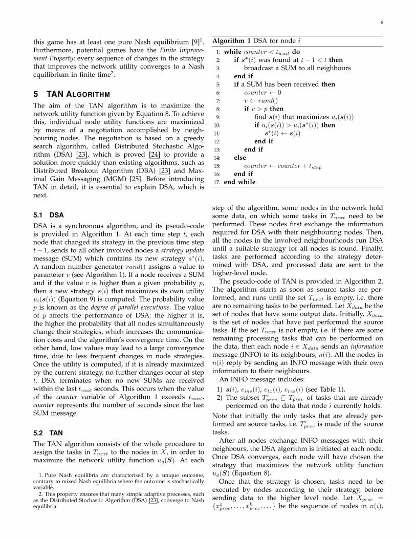
The aim of the TAN algorithm is to maximize thenetwork utility function given by Equation 8. To achievethis, individual node utility functions are maximizedby means of a negotiation accomplished by neigh-bouring nodes. The negotiation is based on a greedysearch algorithm, called Distributed Stochastic Algo-rithm (DSA) [23], which is proved [24] to provide asolution more quickly than existing algorithms, such asDistributed Breakout Algorithm (DBA) [23] and Max-imal Gain Messaging (MGM) [25]. Before introducingTAN in detail, it is essential to explain DSA, which isnext.

5.1 DSA

DSA is a synchronous algorithm, and its pseudo-codeis provided in Algorithm 1. At each time step t, eachnode that changed its strategy in the previous time stept− 1, sends to all other involved nodes a strategy updatemessage (SUM) which contains its new strategy s∗(i).A random number generator rand() assigns a value toparameter v (see Algorithm 1). If a node receives a SUMand if the value v is higher than a given probability p,then a new strategy s(i) that maximizes its own utilityui(s(i)) (Equation 9) is computed. The probability valuep is known as the degree of parallel executions. The valueof p affects the performance of DSA: the higher it is,the higher the probability that all nodes simultaneouslychange their strategies, which increases the communica-tion costs and the algorithm’s convergence time. On theother hand, low values may lead to a large convergencetime, due to less frequent changes in node strategies.Once the utility is computed, if it is already maximizedby the current strategy, no further changes occur at stept. DSA terminates when no new SUMs are receivedwithin the last twait seconds. This occurs when the valueof the counter variable of Algorithm 1 exceeds twait.counter represents the number of seconds since the lastSUM message.

5.2 TAN

The TAN algorithm consists of the whole procedure toassign the tasks in Tnext to the nodes in X , in order tomaximize the network utility function ug(S). At each

1. Pure Nash equilibria are characterised by a unique outcome,contrary to mixed Nash equilibria where the outcome is stochasticallyvariable.

2. This property ensures that many simple adaptive processes, suchas the Distributed Stochastic Algorithm (DSA) [23], converge to Nashequilibria.

Algorithm 1 DSA for node i

1: while counter < twait do2: if s∗(i) was found at t− 1 < t then3: broadcast a SUM to all neighbours4: end if5: if a SUM has been received then6: counter ← 07: v ← rand()8: if v > p then9: find s(i) that maximizes ui(s(i))

10: if ui(s(i)) > ui(s∗(i)) then

11: s∗(i)← s(i)12: end if13: end if14: else15: counter ← counter + tstep16: end if17: end while

step of the algorithm, some nodes in the network holdsome data, on which some tasks in Tnext need to beperformed. These nodes first exchange the informationrequired for DSA with their neighbouring nodes. Then,all the nodes in the involved neighbourhoods run DSAuntil a suitable strategy for all nodes is found. Finally,tasks are performed according to the strategy deter-mined with DSA, and processed data are sent to thehigher-level node.

The pseudo-code of TAN is provided in Algorithm 2.The algorithm starts as soon as source tasks are per-formed, and runs until the set Tnext is empty, i.e. thereare no remaining tasks to be performed. Let Xdata be theset of nodes that have some output data. Initially, Xdata

is the set of nodes that have just performed the sourcetasks. If the set Tnext is not empty, i.e. if there are someremaining processing tasks that can be performed onthe data, then each node i ∈ Xdata sends an informationmessage (INFO) to its neighbours, n(i). All the nodes inn(i) reply by sending an INFO message with their owninformation to their neighbours.

An INFO message includes:1) s(i), eins(i), etx(i), eres(i) (see Table 1).2) The subset T ′prev ⊆ Tprev of tasks that are already

performed on the data that node i currently holds.Note that initially the only tasks that are already per-formed are source tasks, i.e. T ′prev is made of the sourcetasks.

After all nodes exchange INFO messages with theirneighbours, the DSA algorithm is initiated at each node.Once DSA converges, each node will have chosen thestrategy that maximizes the network utility functionug(S) (Equation 8).

Once that the strategy is chosen, tasks need to beexecuted by nodes according to their strategy, beforesending data to the higher level node. Let Xproc =x1proc, . . . , xkproc, . . . be the sequence of nodes in n(i),

7

for which the strategy of node xkproc entails the ex-ecution of processing task tkproc, and let Tproc =t1proc, . . . , tkproc, . . . be the related sequence of process-ing tasks to be performed. Here, the nodes in set Xproc

are ordered according to the order in which the tasks inset Tproc need to be performed, i.e. task tkproc is in the setTin(tk+1

proc). Since a node can perform more than one task,it is possible that two consecutive tasks tkproc and tk+1

proc areexecuted by the same node, i.e. xkproc = xk+1

proc. Each nodexkproc first performs the task tkproc, and updates the setsTnext and Tprev accordingly. Then, if there are no othertasks assigned to it, node xkproc sends a data message(DATA) to node xk+1

proc, to perform task tprock+1. DATA

messages contain the set Tprev , along with the outputdata resulting from task tproc

k.When all the tasks in Tproc are performed, a DATA

message is sent to the higher-level node.Figure 3 shows the sequence of the steps to perform

TAN, for a reference neighbourhood of 3 sensor nodesand a cluster head. Each sketch corresponds to one ofthe basic steps necessary to TAN execution. Node 2 isthe node that has task 1 output data. After the DSAexecution, tasks 2 and 3 are assigned to nodes 3 and 1,respectively. Data is then sent to the cluster head, whichnegotiates with their neighbours for the assignment oftask 4 that is still to be performed.

Algorithm 2 TAN

1: Source tasks are performed2: while Tnext 6= do3: for all i ∈ Xdata do4: send INFO to all nodes in n(i)5: for all j ∈ n(i) do6: send INFO to all nodes in i, n(i)\j7: end for8: for all nodes in i, n(i) do9: execute DSA

10: end for11: for all xkproc ∈ Xproc do12: perform tkproc13: Tnext ← Tnext\tkproc14: Tprev ← Tprev, tkproc15: if xk+1

proc 6= xkproc then16: send DATA to xk+1

proc

17: end if18: end for19: send DATA to the higher-level node20: update Xdata

21: end for22: end while

5.3 Computational Complexity of the Node UtilityFunction MaximizationThe maximization of the node utility function ui(s(i))defined in Equation 9 is a Mixed Integer Linear Pro-gramming problem (MILP) [26]. It is well known that

MILP problems are optimally solved using branch-and-bound algorithms [27], which, in the worst case, have acomplexity that grows exponentially with respect to thenumber of variables. Hence, the complexity of the nodeutility function is related with the number of variables anode uses to compute the function.

Note that the tasks in d(i) are node i’s variablesused for executing TAN. Hence, the number of variablesNvars(i) of node i is equal to the number of tasks it needsto execute, Ntask(i). 3 The number of node i’s tasks isfound by:

Nvars(i) =∑

λ∈Tnext

d(i, λ).

In the worst case, node i is able to perform all thetasks in Tnext, and Tnext is equal to the number ofprocessing tasks in which the application is sub-divided.This means that, in the worst case, Nvars is boundedby |T |. In the worst case, the complexity of maximizingui(s(i)) is equal to the complexity of performing anexhaustive search among all possible combinations ofprocessing assignments, i.e. 2Nvars · Noperations, whereNoperations is the number of operations needed to evalu-ate one node utility function ui(s(i)). It can be estimatedfrom Equation 9 that Noperations ∼ 30 × Nvars, where∼ 30 is the number of operations needed to calculateumark (s(i)) (Equation 10), while Nvars is the numberof times that umark (s(i)) is computed to get ui(s(i)).Note that computational complexity can be considerablyreduced using sub-optimal heuristic algorithms, such asgenetic or tabu-search algorithms.

5.4 Message Complexity of the Node Utility Func-tion Maximization

In this section, the message complexity caused by the ex-change of INFO, SUM, and DATA messages is analysed.

INFO: The INFO message is broadcast within the clus-ter by each node only once. Let Ncluster(i) be the numberof nodes within the cluster that node i belongs to, andlet n(INFO) be the number of bytes required for anINFO message 4. The number of transmitted bytes dueto the exchange of INFO messages for each negotiation istherefore Ncluster ·n(INFO). Typically, Ncluster is around5− 10 [28].

SUM: During the negotiation, a SUM message, whichconsists of |s(i)| boolean values, is broadcast withinthe cluster whenever node i changes its strategy. LetNsteps be the number of steps taken until the negotiationconverges, and let n(SUM) be the number of bytes of aSUM message. In the worst case, at every time step, eachnode in the cluster changes its strategy. Hence, the worstcase number of transmitted bytes for SUM messagesduring each negotiation is Nsteps ·Ncluster · n(SUM).

3. A node i can only perform the tasks that are set in its vector d(i),but not all tasks in Tprev .

4. n(INFO) consists of: |s(i)| boolean values, |eins(i), etxi , eresi |

numeric values, and |T ′prev | identification values.

8

(a) Node 2 ∈ Xdata sends INFO (b) Neighbours send INFO (c) DSA execution

(d) Node 2 sends DATA to x1proc = 3 (e) Node x1proc = 3 sends DATA tox2proc = 1

(f) Node x2proc = 1 sends DATA to theCH

Fig. 3: Sequence of steps to perform TAN. Small nodes represent sensors, whereas the bigger ones are cluster heads(CHs).

DATA: After the negotiation process has converged,a DATA message of n(DATA, k) bytes is sent to eachnode xkproc ∈ Xproc (see Section 5.2), and then to thehigher-level node. The dependence of n(DATA, k) onk is due to the fact that the number of bytes of theoutput data varies based on which task tkproc is executed.n(DATA, k) is proportional to both the amount of outputdata generated by the processed tasks and the number|Tprev| of identification values. In the worst case, eachnode xkproc ∈ Xproc is different from the following onexk+1proc. Therefore, considering that the last DATA message

is sent to the higher-level node (HL), in the worst case,the number of transmitted bytes due to DATA messagesfor each negotiation is

∑k∈Xproc,HL n(DATA, k).

As a result, the worst case number of transmitted bytessent during a single negotiation is:

n(negotiation) =Ncluster · n(INFO)+

Nsteps ·Ncluster · n(SUM)+∑k∈Xproc,HL

n(DATA, k).(11)

Considering the typical case of a network with a num-ber of nodes per cluster Ncluster = 10 [28], and a numberof steps for the negotiation convergence Nsteps = 10 [23],for 30 tasks n(INFO) ∼ 137, and n(SUM) ∼ 16.Therefore, a typical value for the worst case amountof transmitted data per negotiation is n(negotiation) '2.9 kB +

∑k∈Xproc,HL n(DATA, k).

The number of negotiations to perform TAN mainlydepends on the number of hierarchical levels of thenetwork. Suppose that, given an application, all thesource tasks are assigned to sensor nodes within thesame cluster. After each negotiation, data are sent to thehigher level node. Calling L the number of hierarchical

levels, the number of negotiation is at most equal to L−1.On the other hand, if, given an application, all the sourcetasks are assigned to sensor nodes in different clusters,the number of negotiations depends on the number ofsensing tasks as well. In the worst case, for each sensingtask a negotiation is performed in each hierarchical levelexcept the gateway. Therefore, calling M the number ofsensing tasks, the worst case number of negotiations is(L− 1) ·M .

6 PERFORMANCE ANALYSISThe proposed algorithm is tested on hierarchical hetero-geneous WSN scenarios by MATLAB simulations. Themain node parameters are listed in Table 2. More specif-ically, the processing cost parameters found in [3][29],the radio frequency parameters specified in [30], andIEEE 802.15.14 parameters listed in [31] are used. Asdescribed in Section 3.1, although only two kind of nodeshave been considered, i.e. sensors and CHs, the referencearchitecture is characterised by a complex hierarchymade of CHs that control other CHs. Accordingly, thenetwork is made of more than two levels of hierarchydepending on the specific scenario. Specifically, in thesmart city scenario the number of levels is 4 as alsodepicted in Fig. 4; whereas in the random networkscenario it varies in the range 3 ÷ 7 depending on thenode density. In order to take into account heterogeneity,different characteristics of CHs and sensors have beenconsidered: CHs have a maximum processing speed of206 MHz and a residual energy of 4 kJ, while sensornodes have a maximum processing speed of 133 MHzand a residual energy of 2 kJ. The randomly assignedheterogeneous node characteristics are:• non-uniform energy consumption rates: energy con-

sumption parameters are selected randomly in a

9

range from 60% to 140% of the mean values givenin Table 2,

• non-uniform initial energy levels: battery energylevel is assigned randomly from 20% to 100% of themaximum battery capacity,

• non-uniform processing speeds at each node: pro-cessing speed is set randomly from 60% to 100% ofthe highest possible processing speed.

TABLE 2: Simulation parameters

Parameter ValueRF frequency 2400 MHzBit rate 250 kbpsOutput power range ∼ [−24 0] dBmReceiver sensitivity −94 dBmPR0 59.2 mWPT0 26.5 mWη 50%einstr 1 nJPacket header 12 bytesMaximum payload 125 bytesProcessing speed of sensors 133 MHzProcessing speed of CHs 206 MHzInitial energy of sensors 2 kJInitial energy of CHs 4 kJ

In the following, the energy consumption model ispresented. Then, the performance of the TAN algorithmfor two different scenarios are presented. Provided fig-ures present average values over all network nodes.

6.1 Energy Consumption

In this paper, two types of energy consumption at net-work nodes are considered, namely processing energyconsumption and communication energy consumption.

Processing energy consumption eproc depends on twoquantities: the number of instructions, Itask, needed toexecute a task, and the average energy consumption perinstruction einstr(x) at node x. Hence:

eproc(task, x) = Itask · einstr(x). (12)

There are two main components that contribute tocommunication energy consumption: transmission andreception energy consumption [29]. We define the energyper bit necessary to transmit data at rate R from nodex to node y (one-hop neighbours) as etx(x, y), and theper-bit energy consumed for reception of data at node yas erx(y), which are calculated by:

etx(x, y) =1

R

(PT0x +

ϕxy · δγxyηx

),

erx(y) =PR0y

R,

(13)

where PT0x and PR0y are the power consumption com-ponents of the transmitting and receiving circuitry fornode x and node y, respectively. ηx is the drain efficiencyof the power amplifier in x; ϕxy is a coefficient thatis proportional to the minimum reception power anddepends on antenna characteristics; δxy is the distance

between the transmitter and the receiver; and finally, γdenotes the path loss component. These expressions aredescribed in more detail in [29].

6.2 Smart City Scenario

The scenario under examination is that of an urbanenvironment, where nodes are positioned along thestreets as shown in Figure 4. Solid markers representnodes equipped with sensors that measure the speedsof passing-by vehicles, where each speed measurementis represented by a double numerical value (64-bit long).Each street segment is a cluster (as enclosed by a dashedellipse), where CHs are represented by empty markers.CHs are more capable nodes than ordinary sensors (withan initial battery charge twice higher than that of anordinary sensor), and are able to perform the necessarytasks in their clusters, such as local management ofsensors as well as traffic aggregation. CHs do not collectraw data, but process incoming data from the sensors intheir clusters.

Fig. 4: Sample topology for the Smart City Scenario.Solid markers represent nodes equipped with speedsensors, while empty markers are cluster heads. Clustersof sensors are enclosed by dashed ellipses.

Suppose that a driver at point S in Figure 4 wouldlike to know the fastest route to point D, based onthe collected speed information from sensor nodes. Foreach of the 89 sensing nodes, one speed sensing taskis assigned. Since the mean travelling time for eachstreet segment is needed, the collected speed values fromsensors in the same segment are used as input for amean speed computing task. Then, the output of the meanspeed computing tasks, all of which correspond to thesame segment, are given to as input to another task,

10

called the mean travelling time5 computing task, whichprovides the mean value for that segment. To find thebest path, the sum of the mean travelling times of allthe combinations of segments that can be consecutivelydriven is required. This is done by the summation tasks.Finally, the choice of best path task takes the summationvalues related to two merging paths and returns thelower value, i.e. the quicker path. The ordinary nodesin Figure 4 are able to perform speed sensing and meanspeed computing tasks, whereas the CHs are able toperform mean speed computing, mean travelling timecomputing, summation, and choice of best path tasks.Table 3 summarizes the tasks for this scenario.

TABLE 3: Tasks for the Smart City Scenario

Task Description Nodes

Speed sensingSenses the vehicles’ speed. Onespeed sensing task is assigned toeach sensor node

Sensors

Mean speedcomputing

Computes the average of thespeed values collected by speedsensing tasks

Sensors,CHs,node S

Meantravelling timecomputing

Takes the mean speed value relatedto a single segment of a street andreturns the mean travelling time forthat segment

CHs,node S

SummationCalculates the sum of the meantravelling times of two consecutivesegments of a street

CHs,node S

Choice of bestpath

Takes two summation values re-lated to two merging paths andchooses the fastest one

CHs,node S

We simulated the described scenario and comparedthe performance of the proposed algorithm with threealternative approaches:• Mechanism Central: All data is forwarded to and

processed by the gateway (Node S in Figure 4).• Mechanism CO: Data are processed according to

a centralized lifetime optimization algorithm, de-scribed in [2]. In this algorithm, the gateway knowsall the network and application characteristics. Ac-cording to this information, the gateway assignstasks to nodes with the aim of reducing the networkenergy consumption.

• Mechanism DLMA: Data are processed according tothe DLMA algorithm described in [6]. DLMA is adistributed sub-optimal task assignment algorithmwhich aims at improving network lifetime. Contraryto TAN, it only takes into account network lifetime,ignoring the application execution time.

In this way, TAN’s performance is evaluated with respectto static task assignment (mechanism Central), dynamiccentralized optimal task assignment (mechanism CO),and dynamic distributed sub-optimal task assignment(mechanism DLMA).

The obtained results of these mechanisms for energyconsumption and application completion time are com-pared to those obtained using TAN. Figure 5 shows the

5. The mean travelling time is the ratio between the mean speedvalue and the length value related to a segment street.

percent gain of TAN over Central, CO, and DLMA. Werefer to these comparisons as TAN-Central, TAN-CO,and TAN-DLMA.

(a) Energy conservation

(b) Completion time gain

Fig. 5: Percentage values of mean energy conservationand completion time gain using TAN, as compared toTAN-Central, TAN-DLMA, and TAN-CO, for differentvalues of α.

Simulations are run for:• α = 0: null network lifetime component;• α = 1: comparable Ωt and Ωτ ;• α = M , with M 1: null task completion time

component.Significant improvement (around 75%) in energy con-

servation is observed compared to Central. TAN alsoprovides up to 22% gain over Central in applicationcompletion time. When compared to DLMA, TAN showsmoderate gains (up to 15%) in energy conservation, andup to 26% gain in application completion time. Despitethe fact that CO is more energy-efficient than TAN(∼ 12%), TAN achieves its highest gains in applicationcompletion time with respect to CO (up to 35%).

Note that, contrary to TAN, the Central, CO, andDLMA task assignment mechanisms do not take intoaccount the task completion time6, so their performanceare the same irrespective of the value of α. For this rea-son, the most significant results are those obtained when

6. Recall that the task completion time is considered by TAN bymeans of the task completion time component in Equation 1

11

the task completion time (see Equation 2) is negligible,i.e. when α = M . Nevertheless, comparisons for non-infinitesimal values of the task completion time (α = 0and α = 1) are reported for completeness.

As expected, when α increases, which means thatthe utility function is more and more in favour of thenetwork lifetime component, the energy conservationpercentage increases, while the completion time gaindecreases. On the contrary, when α decreases, the utilityfunction is in favour of the task completion time compo-nent, i.e. the energy conservation percentage decreases,while the completion time gain increases.

6.3 Random Network ScenariosApart from the Smart City Scenario of Figure 4, TANis also evaluated for networks with randomly deployedsensors. Sensor locations are uniformly distributed overa rectangular topology, with two key parameters: nodedeployment density and average number of nodes percluster.

The DAG of the application assigned to each networkis obtained by starting with a set of tasks and thenrandomly appending the remaining tasks, while ensur-ing the structure is still a DAG. While doing so, thetotal number of tasks is fixed. The number of instruc-tions required to perform each task and the number ofoutput bits for each task are set randomly accordingto a uniform distribution from 2.7 · 105 to 3.3 · 105,and from 720 bits to 880 bits, respectively [32]. Theapplication deadline is fixed and is set to 80 ms [3]. Theability of each node to perform a task7 (the values ofthe elements corresponding to the tasks of each vectord(i) described in Section 3.2) is assigned according toa task distribution parameter. This parameter defines theprobability of each node to be able to perform a giventask8. Table 4 summarises the evaluation parameters.

TABLE 4: Characteristic Parameters Values for RealisticRandom Scenarios

Parameter Min Default MaxNode density [nodes/m2] 0.2 0.3 0.4Number of nodes per cluster 5 15 25Number of tasks 10 20 30Distribution of tasks 10% 50% 100%

Note that the Smart City Scenario corresponds to a net-work with a low node density of around 0.15 nodes/m2,a low number of nodes per cluster, which is around 8nodes/cluster, a high number of tasks equal to 100, anda very low task distribution parameter of about 6.9%. Inthe following, the performance of TAN algorithm whenthese parameters change is discussed and compared to

7. In the following, the word task is referred to as tasks in Tnext atthe initial instant. Since sensing tasks do not affect TAN performance,they are not considered as a critical parameter.

8. Note that this is different from d(i), which is a vector of booleanvalues denoting the ability of node i to perform individual tasks, butnot the probability of the ability to execute the tasks.

C, CO and DLMA. The results also include a comparisonbetween TAN and the mechanism in which all the dataare sent to the gateway and processed only by thegateway (mechanism Central in the Smart City Scenario).

0.2 0.25 0.3 0.35 0.4 1

1.5

2

2.5

3

3.5

4

4.5

Node density [nodes/m2]

Ave

rag

e en

erg

y co

nsu

mp

tio

n [

mJ]

TAN, α=0TAN, α=1TAN, α=MDLMACOCentral

(a) Average energy consumption

0.2 0.25 0.3 0.35 0.4 55

60

65

70

75

80

85

90

Node density [nodes/m2]

Ave

rag

e ap

plic

atio

n c

om

ple

tio

n t

ime

[ms]

TAN, α=0TAN, α=1TAN, α=MDLMACOCentral

Application deadline

(b) Average application completion time

Fig. 6: Average energy consumption and applicationcompletion time for TAN, DLMA, CO, and Central taskassignment mechanisms for different node densities.

6.3.1 The Effect of Node Density

In this set of simulations, the aim is to observe thealgorithm performance when the inter-node distanceschange due to the change in node deployment density.Figure 6 shows how the averages of overall energyconsumption and application completion time changewhen node density is altered, for different values ofthe weighting factor α of Equation 1. Figure 6 alsoreports the confidence intervals for the average energyconsumption and application completion time at a 95%.

In Figure 6(a), since the network lifetime component(Equation 3) depends on the hop distance to the higherlevel node due to multihop data transmission, we ob-serve an improvement in energy consumption when αincreases. For non-zero values of α, slight improvementin energy conservation is observed for increasing nodedensity. This is due to the fact that, when node density

12

increases, the energy consumption due to the messageexchanges of negotiations is lower. Note that whenα = 0, the network lifetime component is not taken intoaccount for choosing the best strategy, and this can beobserved in the flatness of the related curve.

In Figure 6(b), some improvement in application com-pletion time is observed with increasing node density.Although TAN (and all the other mechanisms) is outper-formed by the optimal CO algorithm in terms of energyconsumption, a gain of up to ∼20 msec is achieved byTAN when compared to CO, with respect to applicationcompletion time.

5 10 15 20 25 1

1.5

2

2.5

3

3.5

4

4.5

5

Nodes/cluster

Ave

rag

e en

erg

y co

nsu

mp

tio

n [

mJ]

TAN, α=0TAN, α=1TAN, α=MDLMACOCentral

(a) Average energy consumption

5 10 15 20 25 55

60

65

70

75

80

85

90

Nodes/cluster

Ave

rag

e ap

plic

atio

n c

om

ple

tio

n t

ime

[ms]

TAN, α=0TAN, α=1TAN, α=MDLMACOCentral

Application deadline

(b) Average application completion time

Fig. 7: Average energy consumption and applicationcompletion time for TAN, DLMA, CO, and Central taskassignment mechanisms for different number of nodesper cluster.

6.3.2 The Effect of the Number of Nodes in ClustersThe second set of simulations evaluates the effect ofthe average number of nodes in a cluster on TAN’sperformance. In Figure 7, the overall energy consump-tion and application completion time variations andtheir related 95% confidence intervals are shown withrespect to different values of α and different number ofnodes per cluster. It can be observed that the effect ofhaving more nodes in a cluster on TAN’s performance is

similar to what is observed for the effect of node densityincrease. This can be attributed to the fact that TANis mostly affected by how many nodes fall in a clus-ter’s boundary, which directly affects its task allocationstrategy. Note that TAN’s negotiations are performedamong neighbouring nodes within the same cluster. Anincrement in density or nodes per cluster is equivalentto an increasing node degree. This helps TAN refine thequality of its negotiation results at each algorithm stepand eventually reduces algorithm convergence time andthe total energy consumption.

6.3.3 The Effect of the Number of Tasks

In order to evaluate TAN’s performance at processingapplications with different complexities, the number oftasks in an application is varied, while keeping the ap-plication deadline fixed. By doing so, the available timeper task is effectively reduced. This in turn affects theapplication completion time component of Equation 1.

Figure 8 demonstrates the effect of the applicationcomplexity, and the 95% confidence intervals. We ob-serve a noticeable improvement in both energy con-sumption and completion time when the number oftasks increases from 10 to 20. This is due to the fact that,for a low number of tasks such as 10, the results foran optimized strategy can not be much different fromthe case where all tasks are assigned to the gateway.One observation in Figure 8(b) is that TAN providesthe shortest application completion times for all studiedcases of application complexity. TAN with α = 0 hasa high consumption due to the fact that when α = 0the network lifetime component is not considered inEquation 1. Among all, CO has the least consumption,thanks to its ability to find the optimal solution withrespect to the average energy consumption.

6.3.4 The Effect of the Task Distribution Parameter

In the last set of simulations, the effect of the taskdistribution parameter is studied. Recall that this valuecorresponds to the probability of a node to be able toperform a task. Figure 9 shows TAN performance ofthe algorithms. Noticeable improvement both in overallenergy consumption and in application completion timeusing TAN is noticed when it is possible to assign moretasks to nodes, and the best results are obtained whenthe network is able to perform every task.

In the Smart City Scenario, the task distribution pa-rameter is set to 6.9%, which is extremely low whencompared to those of the random network scenarios.Nevertheless, the performance of TAN in random net-works is worse compared to that in the Smart Cityscenario. This is due to the fact that, for the SmartCity scenario, the ability of each node to perform atask is strictly related to the task (as opposed to beingrandomly assigned). Therefore, only the nodes that aremore suitable to perform a given task have the ability toexecute that task.

13

10 15 20 25 30 1

1.5

2

2.5

3

3.5

4

4.5

5

Number of processing tasks

Ave

rag

e en

erg

y co

nsu

mp

tio

n [

mJ]

TAN, α=0TAN, α=1TAN, α=MDLMACOCentral

(a) Average energy consumption

10 15 20 25 30 30

40

50

60

70

80

90

100

110

Number of processing tasks

Ave

rag

e ap

plic

atio

n c

om

ple

tio

n t

ime

[ms]

TAN, α=0TAN, α=1TAN, α=MDLMACOCentral

Application deadline

(b) Average application completion time

Fig. 8: Average energy consumption and applicationcompletion time for TAN, DLMA, CO, and Central taskassignment mechanisms for different number of tasks.

7 CONCLUSIONS

In this paper, we propose TAN, a distributed algorithmfor dynamic task assignment in heterogenous WSNs,which aims at maximizing network lifetime while en-suring that application completion time is as short aspossible. TAN is tested in two reference scenarios: (i) aSmart City environment, and (ii) a set of random sce-narios with different characteristics. TAN has shownto outperform gateway-oriented and DLMA-orientedmechanisms in terms of both energy conservation andapplication completion time. TAN is only outperformedin terms of energy conservation by the tested centralizedalgorithm, which however is considerably more complexand cannot meet application deadlines due to its longapplication completion time.

In all scenarios, the average node energy consumptionusing TAN is found to be inversely proportional to aweighting factor α that strikes the balance between twoconflicting goals: a long network lifetime and a shortapplication completion time. In particular, the α valueis found to be more critical for scenarios with complexapplications, where the application deadline is morelikely to be missed.

10% 30% 50% 75% 100% 0

0.5

1

1.5

2

2.5

3

3.5

4

4.5

Task distribution parameter

Ave

rag

e en

erg

y co

nsu

mp

tio

n [

mJ]

TAN, α=0TAN, α=1TAN, α=MDLMACOCentral

(a) Average energy consumption

10% 30% 50% 75% 100% 40

50

60

70

80

90

Task distribution parameter

Ave

rag

e ap

plic

atio

n c

om

ple

tio

n t

ime

[ms]

TAN, α=0TAN, α=1TAN, α=MDLMACOCentral

Application deadline

(b) Average application completion time

Fig. 9: Average energy consumption and applicationcompletion time for TAN, DLMA, CO, and Central taskassignment mechanisms for different values of the taskdistribution parameter.

TAN characteristics make it perfectly suitable not onlyfor WSNs, but also for multi-technology IoT scenarios.Using TAN, the adaptive IoT network components co-operate dynamically in order to achieve optimal per-formance. Furthermore, with little changes to the taskutility function, other requirements such as Quality ofService (QoS) may be optimized.

REFERENCES

[1] L. Atzori, A. Iera, and G. Morabito, “The internet of things: Asurvey,” Computer Networks, vol. 54, no. 15, pp. 2787 – 2805, 2010.

[2] V. Pilloni and L. Atzori, “Deployment of distributed applicationsin wireless sensor networks,” Sensors, vol. 11, no. 8, pp. 7395–7419,2011.

[3] Y. Jin, J. Jin, A. Gluhak, K. Moessner, and M. Palaniswami, “An in-telligent task allocation scheme for multihop wireless networks,”Parallel and Distributed Systems, IEEE Transactions on, pp. 444–451,2012.

[4] J. Zhu, J. Li, and H. Gao, “Tasks allocation for real-time appli-cations in heterogeneous sensor networks for energy minimiza-tion,” in Proceedings of the Eighth ACIS International Conference onSoftware Engineering, Artificial Intelligence, Networking, and Paral-lel/Distributed Computing, vol. 2, 2007, pp. 20–25.

14

[5] S. Abdelhak, C. Gurram, S. Ghosh, and M. Bayoumi, “Energy-balancing task allocation on wireless sensor networks for extend-ing the lifetime,” in Circuits and Systems (MWSCAS), 2010 53rdIEEE International Midwest Symposium on, 2010, pp. 781 –784.

[6] V. Pilloni, M. Franceschelli, L. Atzori, and A. Giua, “A decentral-ized lifetime maximization algorithm for distributed applicationsin wireless sensor networks,” in Communications (ICC), 2012 IEEEInternational Conference on, 2012, pp. 1392–1397.

[7] Y. Shen and H. Ju, “Energy-efficient task assignment based onentropy theory and particle swarm optimization algorithm forwireless sensor networks,” in Green Computing and Communica-tions (GreenCom), 2011 IEEE/ACM International Conference on, 2011,pp. 120 –123.

[8] K. Ritzberger, Foundations of non-cooperative game theory. OxfordUniversity Press, 2002.

[9] D. Monderer and L. Shapley, “Potential games,” Games and eco-nomic behavior, vol. 14, pp. 124–143, 1996.

[10] D. Wang, B. Xie, and D. Agrawal, “Coverage and lifetime opti-mization of wireless sensor networks with gaussian distribution,”Mobile Computing, IEEE Transactions on, vol. 7, no. 12, pp. 1444–1458, 2008.

[11] J. Luo, J. Panchard, M. Piorkowski, M. Grossglauser, andJ. Hubaux, “Mobiroute: Routing towards a mobile sink for im-proving lifetime in sensor networks,” Distributed Computing inSensor Systems, pp. 480–497, 2006.

[12] X. Xu and W. Liang, “Placing optimal number of sinks in sensornetworks for network lifetime maximization,” in Communications(ICC), 2011 IEEE International Conference on, 2011, pp. 1–6.

[13] W. Heinzelman, A. Chandrakasan, and H. Balakrishnan, “Anapplication-specific protocol architecture for wireless microsensornetworks,” IEEE Transactions on Wireless Communications, vol. 1,pp. 660–670, October 2002.

[14] D. Wei, Y. Jin, S. Vural, and R. Tafazolli, “An energy-efficient clus-tering solution for wireless sensor networks,” IEEE Transactions onWireless Communications, vol. 10, no. 11, pp. 3973–3983, Nov. 2011.

[15] Y. Yu and V. K. Prasanna, “Energy-balanced task allocation forcollaborative processing in wireless sensor networks,” MobileNetworks and Applications, vol. 10, pp. 115–131, 2005.

[16] N. Edalat, W. Xiao, C. Tham, E. Keikha, and L. Ong, “A price-based adaptive task allocation for wireless sensor network,” inMobile Adhoc and Sensor Systems, 2009. MASS’09. IEEE 6th Inter-national Conference on, 2009, pp. 888–893.

[17] B. Kaleci, O. Parlaktuna, M. Ozkan, and G. Kirlik, “Market-basedtask allocation by using assignment problem,” in Systems Man andCybernetics (SMC), 2010 IEEE International Conference on. IEEE,2010, pp. 135–141.

[18] P. Sujit, A. Sinha, and D. Ghose, “Team, game, and negotiationbased intelligent autonomous uav task allocation for wide areaapplications,” in Innovations in Intelligent Machines-1. Springer,2007, pp. 39–75.

[19] J. N. Al-karaki and A. E. Kamal, “Routing techniques in wirelesssensor networks: A survey,” IEEE Wireless Communications, vol. 11,pp. 6–28, 2004.

[20] Q. Li, J. Aslam, and D. Rus, “Hierarchical power-aware routingin sensor networks,” in In Proceedings of the DIMACS Workshop onPervasive Networking, 2001.

[21] A. C. Chapman, R. A. Micillo, R. Kota, and N. R. Jennings, “De-centralised dynamic task allocation: A practical game-theoreticapproach,” in Proc. of the 8th International Conference on AutonomousAgents and Multiagent Systems, vol. 2, 2009, pp. 915–922.

[22] G. Arslan, J. R. Marden, and J. S. Shamma, “Autonomous vehicle-target assignment: A game-theoretical formulation,” Journal ofDynamic Systems, Measurement, and Control, vol. 129, no. 5, pp.584–596, 2007.

[23] W. Zhang, G. Wang, Z. Xing, and L. Wittenburg, “Distributedstochastic search and distributed breakout: properties, compar-ison and applications to constraint optimization problems insensor networks,” Artificial Intelligence, vol. 161, no. 1-2, pp. 55– 87, 2005.

[24] M. Vinyals, J. Rodriguez-Aguilar, and J. Cerquides, “A survey onsensor networks from a multiagent perspective,” The ComputerJournal, vol. 54, no. 3, pp. 455–470, 2011.

[25] J. P. Pearce and M. Tambe, “Quality guarantees on k-optimalsolutions for distributed constraint optimization problems,” inProceedings of the 20th international joint conference on Artificalintelligence, 2007, pp. 1446–1451.

[26] M. Conforti, G. Cornuejols, and G. Zambelli, “Polyhedral ap-proaches to mixed integer linear programming,” 50 Years of IntegerProgramming 1958-2008, pp. 343–385, 2010.

[27] E. Lawler and D. Wood, “Branch-and-bound methods: A survey,”Operations research, vol. 14, no. 4, pp. 699–719, 1966.

[28] N. Vlajic and D. Xia, “Wireless sensor networks: to cluster or notto cluster?” in World of Wireless, Mobile and Multimedia Networks,2006. WoWMoM 2006. International Symposium on a. IEEE, 2006,pp. 9–pp.

[29] Q. Wang and W. Yang, “Energy consumption model for powermanagement in wireless sensor networks,” in IEEE Sensor, Meshand Ad Hoc Communications and Networks (SECON) 2007, 2007, pp.142 –151.

[30] Chipcon, “Smartrf cc2420 datasheet,” 2.4GHz IEEE802.15.4/ZigBee-ready RF transceiver.

[31] IEEE, “Std 802.15.4TM,” 2006, wireless Medium Access Control(MAC) and Physical Layer (PHY) Specifications for Low-RateWireless Personal Area Networks (WPANs).

[32] Y. Tian and E. Ekici, “Cross-layer collaborative in-network pro-cessing in multihop wireless sensor networks,” Mobile Computing,IEEE Transactions on, vol. 6, no. 3, pp. 297–310, 2007.