
Lab Color Sense - Repositório Aberto da Universidade do Porto
Upload
khangminh22Category
view
3download
0
FACULDADE DE ENGENHARIA DA UNIVERSIDADE DO PORTO
Improving QoS for Large Scale WSNs
Ricardo Augusto Rodrigues da Silva Severino
Doctoral Programme in Electrical and Computer Engineering
Supervisor: Prof. Eduardo Manuel Medicis Tovar
Second Supervisor: Prof. Nuno Alexandre Magalhães Pereira
December 16, 2015

c© Ricardo Augusto Rodrigues da Silva Severino, 2015

Improving QoS for Large Scale WSNs
Ricardo Augusto Rodrigues da Silva Severino
Doctoral Programme in Electrical and Computer Engineering
Approved by:
President: Dr. José Alfredo Ribeiro da Silva MatosExternal Referee: Dr. Vlado HandzinskiExternal Referee: Dr. Leandro Buss BeckerInternal Referee: Dr. Paulo José Lopes Machado Portugal
Internal Referee: Dr. Manuel Alberto Pereira RicardoSupervisor: Dr. Eduardo Manuel Medicis Tovar
December 16, 2015


Resumo
Os avanços nas tecnologias da informação e das comunicações têm possibilitado um aumento ex-ponencial na sua miniaturização e ubiquidade, abrindo caminho a novos paradigmas nos sistemascomputacionais embebidos. Estes avanços, viabilizaram um conjunto de dispositivos mais pequenos,mais inteligentes e ubíquos, alimentando uma vontade de monitorizar e controlar tudo, em qualquerlugar.
Este facto tem vindo a impulsionar o desenvolvimento de novas infra-estruturas de redes sensoriaissem fios (WSN) que irão interagir de uma forma muito próxima com o meio envolvente, de uma formaubíqua e pervasiva. Contudo, estes sistemas ciber-físicos requerem uma reavaliação dos conceitostradicionais da computação e das comunicações, com especial preponderância no que diz respeito àssuas características temporais. Contudo, para além dessa, existem outras vertentes de Qualidade deServiço (QoS), como escalabilidade, eficiência energética, e robustez, que têm de ser consideradaspara que estas infra-estruturas se tornem uma realidade.
Esta dissertação, tem por objectivo desenvolver infra-estruturas de WSNs, capazes de responderaos requisitos de QoS que os futuros sistemas embebidos de grande escala deverão exigir. Isto, atravésda utilização de protocolos normalizados, em particular do IEEE 802.15.4 e ZigBee, em conjunto comtecnologias comerciais. Com este propósito, nesta tese são propostas diversas soluções (mecanismos,algoritmos, protocolos) para resolver alguns dos maiores desafios em termos de QoS nestas infra-estruturas, nomeadamente: comportamento temporal, escalabilidade, robustez e eficiência energética.
De forma a identificar claramente estes desafios de QoS, e a desenvolver soluções em proximi-dade com a realidade, apostou-se numa orientação com uma forte componente prática. Assim, estatese debruça-se sobre dois cenários reais (i.e. monitorização de um datacenter e monitorização de es-truturas), que foram desenvolvidos e implementados de forma a demonstrar as propostas apresentadasnesta dissertação. Esta estratégia, permite uma avaliação destas propostas num contexto aplicacional,demonstrando o potencial destas infra-estruturas para suportar as aplicações ciber-físicas do futuro,quando complementadas com os necessários mecanismos de gestão de QoS.
Relativamente ao comportamento temporal, por exemplo, são conhecidas as vantagens das redesZigBee baseadas em topologias cluster-tree. Contudo, estas apresentam limitações em termos deflexibilidade. O seu funcionamento, normalmente estático, impede a redistribuição da largura debanda atribuída a um conjunto de nós ou, o reajuste da ordem do seu escalonamento de modo areduzir a latência nas comunicações. Assim, nesta tese é proposto um mecanismo para reordenaros períodos activos dos diversos clusters de uma forma dinâmica, durante o funcionamento da rede.Na sub-camada MAC do IEEE 802.15.4, o comportamento temporal também é considerado. Nestesentido, nesta tese é feita uma avaliação experimental de um mecanismo de diferenciação de tráfego.Este mecanismo é também estendido para suportar comunicações intra-cluster. Também se apontamvantagens na sua utilização de um ponto de vista da eficiência energética.
i

ii
Ainda no contexto do comportamento temporal, implementou-se o mecanismo de GuaranteedTime Slots (GTS) do protocolo IEEE 802.15.4 em TinyOS, de modo a garantir comunicações emtempo-real para as aplicações.
A escalabilidade destas infra-estruturas é endereçada nesta tese, através da proposta de um mecan-ismo que permite uma sincronização inter-cluster numa rede ZigBee para um determinado instantetemporal. Este mecanismo permite, nomeadamente, que uma aplicação de monitorização estruturalpossa ser estendida a vários clusters.
Em cenários cuja infra-estrutura de rede é bastante dinâmica, a robustez é normalmente um de-safio, particularmente quando se pretende que uma rede se adapte a diferentes fluxos de tráfego semintervenção humana. Neste sentido, nesta dissertação, propõe-se um mecanismo automático, de múlti-plas camadas, que efectua uma monitorização periódica de um conjunto de indicadores de perfor-mance, e actua em seguida nos mecanismos de QoS respectivos. Este mecanismo, o Traffic EfficiencyControl Module (TECM), permite melhorar a probabilidade sucesso nas transmissões bem como min-imizar os requisitos de memória e latências na rede, através de uma escolha cuidadosa dos parâmetrosdo algoritmo de CSMA-CA do IEEE 802.15.4 e de uma alocação eficiente de largura de banda paracada cluster.

Abstract
The advancements in information and communication technologies have been triggering an increase inminiaturization and ubiquity, paving the way towards new paradigms in embedded computing systems.Modern embedded systems are enabling a number of smaller, smarter and ubiquitous devices, creatingan eagerness for monitoring and controlling everything, everywhere.
These facts are pushing forward the design of new Wireless Sensor Network (WSN) infrastruc-tures that will tightly interact with the physical environment, in a ubiquitous and pervasive fashion.However, such cyber-physical systems require a rethinking of the usual computing and networkingconcepts, and given that these computing entities closely interact with their environment, timelinessis of increasing importance. Nevertheless, many other QoS properties such as scalability, energy-efficiency and robustness must also be addressed if these infrastructures are to become a reality.
This Thesis addresses the use of standard protocols, particularly IEEE 802.15.4 and ZigBee, com-bined with commercial technologies as a baseline to enable WSN infrastructures capable of support-ing the QoS requirements that future large-scale networked embedded systems will impose. Hence,several architectural solutions (mechanisms, algorithms, protocol add-ons) are hereby proposed toaddress some of the most prominent QoS challenges, such as timeliness, scalability, robustness andenergy-efficiency.
Importantly, in order to clearly identify the most prominent QoS challenges and to provide effec-tive QoS solutions with close contact with reality, a hands-on approach is followed throughout thisThesis. Hence, we rely upon two real-world application scenarios (i.e. a Datacentre Monitoring (DM)scenario and a Structural Health Monitoring (SHM) scenario), which were engineered, implementedand deployed in the course of this work, to validate and demonstrate this Thesis’ QoS proposals. Thisstrategy enables a deeper understanding of these infrastructures at a more practical level, and providesthe proposals with a real-world application context, showing that these network infrastructures havethe potential to be used in real-world cyber-physical applications in the near future, if provided withthe necessary QoS management mechanisms.
Among the proposals, concerning timeliness, for instance, ZigBee cluster-tree topologies areknown for a lack of flexibility in adapting to changes in the traffic or bandwidth requirements at run-time, making these infrastructures not capable of allocating more bandwidth to a set of nodes sensing aparticular phenomena, or reducing the latency of a data stream. This Thesis proposes a way of dynam-ically addressing this problem via a mechanism to re-schedule the clusters’ active periods. Concerningthe MAC sub-layer of the IEEE 802.15.4 protocol, in this Thesis we carry out an experimental eval-uation of a traffic differentiation mechanism, providing the support of different traffic classes to thelegacy protocol. This mechanism is also extended to support intra-cluster communications. In ad-dition to timeliness, this mechanism provides and improvement in terms of energy-efficiency. TheIEEE 802.15.4 Guaranteed Time Slot mechanism, missing from most stack implementations, is also
iii

iv
implemented over the TinyOS operating system, providing real-time traffic support to TinyOS-basedapplications.
Scalability is also addressed in this Thesis with the proposal of a mechanism to support inter-cluster synchronization, enabling nodes within multiple clusters in a ZigBee cluster-tree topology tosynchronize to one specific point in time. This mechanism is mandatory, for instance, to scale a SHMsystem to multiple clusters.
In scenarios where the network is quite dynamic, robustness is usually a challenge, particularlyin making a network adapt to different traffic flows or timeliness requirements without human inter-ference. In this line, to address robustness in these network infrastructures, this Thesis proposes anon-line and cross-layer Traffic Efficiency Control Module (TECM) to carry out a periodic monitoringof a set of performance indicators, and to act upon the necessary QoS mechanisms. This mechanismis able to improve the probability of successful transmissions and minimize memory requirements andqueuing delays, through a careful tuning of the IEEE 802.15.4 Slotted CSMA-CA parameters and bycarrying out an efficient bandwidth allocation at the network clusters.

Acknowledgements
I would like to express my deepest gratitude to my supervisor Dr. Eduardo Tovar, for his inspirationand advice. The freedom he granted me in my research work together with his guidance helped me togrow and mature in my work. I would also like to thank my co-supervisor in this Thesis, Dr. NunoPereira, for his insights within the SENODs project and in the Dynamic Cluster Scheduling proposal.
I could not forget to thank Dr. Mário Alves. It was by his hand I gave my first steps into researchwork. Thank you for always being there, for your contagious motivation and for your patience.
Research is naturally incremental and much of the work carried out builds over important contri-butions from great researchers I had the pleasure to work with in the past such as Dr. Anis Koubaaand Dr. Petr Jurcik. Both hard working researchers to which I owe much of what I learned on Wire-less Sensor Networks. A special thanks to another great researcher, Dr. Stefano Tennina, for havingalways been ready to give a hand on the Open-ZB implementation and simulation code, and for hisalways helpful insights.
Team work was a key point in this Thesis. It is amazing what so few people can achieve in solittle time when they join efforts into a project. Therefore, within the SENOD’s project team, a specialmention to Bruno Saraiva, for all the effort and long hours we spent together into making everythingwork on time, to fulfil those always tight deadlines. Within the structural health monitoring projectteam, a big thanks to Ricardo Gomes for his astonishing hardware work and his patience throughoutall of the many system debugging hours. Also to Rafael Aguilar at the ISISE at the University ofMinho, for the technical insights and the time he invested into the system’s evaluation.
A big thanks to Dr. Raghuraman Rangarajan, for his reviewing work and patience, in goingthrough all of this Thesis.
I would also like to thank all the people in the CISTER Research Center at ISEP/IPP, for theirsupport and enthusiasm. Those moments we shared during lunch time, were priceless and importantfor my sanity. Also a big thanks to the administrative staff at CISTER for all their support throughoutthe many bureaucratic details, and to CISTER’s helpdesk team.
To my friends, a big hug and thanks for their encouragement and support. Even though a fewmight be quite far away, they never leave my heart.
I would like to thank my parents for the love, encouragement and support they always providedme through my entire life. I owe more to them than I could ever repay.
Finally, I cannot thank enough my wife Rute for her deep affection, true love, and encouragementthroughout all of this time, and for inspiring me when I needed the most.
Ricardo Severino
v

vi
This work was supported by FCT (Fundação para a Ciência e Tecnologia) under the PhD grantSFRH / BD / 71573 / 2010

“Start by doing what’s necessary;then do what’s possible;
suddenly you are doing the impossible.”
Francis of Assisi
vii

viii

Contents
I Introduction 1
1 Context and Motivation 31.1 Research Context . . . . . . . . . . . . . . . . . . . . . . . . . . . . . . . . . . . . 31.2 Challenges . . . . . . . . . . . . . . . . . . . . . . . . . . . . . . . . . . . . . . . . 51.3 Approach . . . . . . . . . . . . . . . . . . . . . . . . . . . . . . . . . . . . . . . . 71.4 Thesis Statement . . . . . . . . . . . . . . . . . . . . . . . . . . . . . . . . . . . . 81.5 Contributions . . . . . . . . . . . . . . . . . . . . . . . . . . . . . . . . . . . . . . 81.6 Outline . . . . . . . . . . . . . . . . . . . . . . . . . . . . . . . . . . . . . . . . . 11
2 Overview of the IEEE 802.15.4 and ZigBee Protocols 132.1 The ZigBee Protocol . . . . . . . . . . . . . . . . . . . . . . . . . . . . . . . . . . 14
2.1.1 General Aspects . . . . . . . . . . . . . . . . . . . . . . . . . . . . . . . . 142.1.2 The case for the Cluster-tree Topology . . . . . . . . . . . . . . . . . . . . . 172.1.3 The ZigBee Network Layer . . . . . . . . . . . . . . . . . . . . . . . . . . 18
2.2 Overview of the IEEE 802.15.4 Protocol . . . . . . . . . . . . . . . . . . . . . . . . 272.2.1 Physical Layer . . . . . . . . . . . . . . . . . . . . . . . . . . . . . . . . . 282.2.2 Medium Access Control (MAC) Sub-layer . . . . . . . . . . . . . . . . . . 29
2.3 A Review of Other Standard Protocols for WSNs . . . . . . . . . . . . . . . . . . . 39
3 Technological Platforms and Tools 453.1 WSN Platforms and Development Tools . . . . . . . . . . . . . . . . . . . . . . . . 45
3.1.1 Mote Platforms . . . . . . . . . . . . . . . . . . . . . . . . . . . . . . . . . 463.1.2 IEEE 802.15.4/ZigBee Protocol Analysers . . . . . . . . . . . . . . . . . . 47
3.2 WSN Operating Systems . . . . . . . . . . . . . . . . . . . . . . . . . . . . . . . . 493.2.1 TinyOS . . . . . . . . . . . . . . . . . . . . . . . . . . . . . . . . . . . . . 503.2.2 ERIKA Real-time Operating System . . . . . . . . . . . . . . . . . . . . . . 52
3.3 IEEE 802.15.4/ZigBee Protocol Stacks . . . . . . . . . . . . . . . . . . . . . . . . . 523.3.1 Open-ZB Protocol Stack for TinyOS . . . . . . . . . . . . . . . . . . . . . . 533.3.2 Open-ZB Protocol Stack for ERIKA . . . . . . . . . . . . . . . . . . . . . . 573.3.3 The Official TinyOS v2.x IEEE 802.15.4/ZigBee Protocol Stack . . . . . . . 59
3.4 The Open-ZB IEEE 802.15.4 Simulation Model . . . . . . . . . . . . . . . . . . . . 62
ix

x CONTENTS
II On the Engineering of WSN enabled Cyber-physical Applications 65
4 IEEE 802.15.4 GTS Implementation in TinyOS 674.1 Introduction . . . . . . . . . . . . . . . . . . . . . . . . . . . . . . . . . . . . . . . 674.2 Overview of the IEEE 802.15.4 GTS Mechanism . . . . . . . . . . . . . . . . . . . 684.3 Implementation Details . . . . . . . . . . . . . . . . . . . . . . . . . . . . . . . . . 68
4.3.1 Overview . . . . . . . . . . . . . . . . . . . . . . . . . . . . . . . . . . . . 684.3.2 GTS Allocation . . . . . . . . . . . . . . . . . . . . . . . . . . . . . . . . . 714.3.3 GTS Buffer Management . . . . . . . . . . . . . . . . . . . . . . . . . . . . 724.3.4 GTS Deallocation . . . . . . . . . . . . . . . . . . . . . . . . . . . . . . . . 74
4.4 Test and validation . . . . . . . . . . . . . . . . . . . . . . . . . . . . . . . . . . . 744.5 Final Remarks . . . . . . . . . . . . . . . . . . . . . . . . . . . . . . . . . . . . . . 76
5 Structural Health Monitoring Application Scenario 775.1 Context and Motivation . . . . . . . . . . . . . . . . . . . . . . . . . . . . . . . . . 775.2 Related Work . . . . . . . . . . . . . . . . . . . . . . . . . . . . . . . . . . . . . . 785.3 System Overview . . . . . . . . . . . . . . . . . . . . . . . . . . . . . . . . . . . . 80
5.3.1 System Requirements . . . . . . . . . . . . . . . . . . . . . . . . . . . . . 805.3.2 Snapshot of the System Architecture . . . . . . . . . . . . . . . . . . . . . . 81
5.4 Hardware Platform and Signal Acquisition Sub-system . . . . . . . . . . . . . . . . 825.5 WSN Architecture . . . . . . . . . . . . . . . . . . . . . . . . . . . . . . . . . . . 83
5.5.1 Guaranteeing Synchronization . . . . . . . . . . . . . . . . . . . . . . . . . 845.5.2 Communication Architecture . . . . . . . . . . . . . . . . . . . . . . . . . . 845.5.3 Coordinator node . . . . . . . . . . . . . . . . . . . . . . . . . . . . . . . . 865.5.4 Sensing Nodes . . . . . . . . . . . . . . . . . . . . . . . . . . . . . . . . . 87
5.6 Test and Validation . . . . . . . . . . . . . . . . . . . . . . . . . . . . . . . . . . . 885.6.1 Command and Configuration Application . . . . . . . . . . . . . . . . . . . 885.6.2 SHM System Validation . . . . . . . . . . . . . . . . . . . . . . . . . . . . 89
5.7 Final Remarks . . . . . . . . . . . . . . . . . . . . . . . . . . . . . . . . . . . . . . 92
6 Datacenter Monitoring Application Scenario 956.1 Context and Motivation . . . . . . . . . . . . . . . . . . . . . . . . . . . . . . . . . 956.2 Related Work . . . . . . . . . . . . . . . . . . . . . . . . . . . . . . . . . . . . . . 976.3 Architecture Overview . . . . . . . . . . . . . . . . . . . . . . . . . . . . . . . . . 99
6.3.1 Environment and Power Data Collection . . . . . . . . . . . . . . . . . . . . 996.3.2 Data Distribution . . . . . . . . . . . . . . . . . . . . . . . . . . . . . . . . 108
6.4 Mapping The World . . . . . . . . . . . . . . . . . . . . . . . . . . . . . . . . . . . 1086.5 The Data Center Radio Environment . . . . . . . . . . . . . . . . . . . . . . . . . . 1106.6 Final Remarks . . . . . . . . . . . . . . . . . . . . . . . . . . . . . . . . . . . . . . 114
III QoS Improvement Mechanisms 117
7 Peformance Evaluation of a Traffic Differentiation Mechanism 1197.1 Introduction . . . . . . . . . . . . . . . . . . . . . . . . . . . . . . . . . . . . . . . 1197.2 Related Work . . . . . . . . . . . . . . . . . . . . . . . . . . . . . . . . . . . . . . 121

CONTENTS xi
7.3 Traffic Differentiation Strategy . . . . . . . . . . . . . . . . . . . . . . . . . . . . . 1237.4 Implementation Approach . . . . . . . . . . . . . . . . . . . . . . . . . . . . . . . 1247.5 Performance Evaluation . . . . . . . . . . . . . . . . . . . . . . . . . . . . . . . . . 126
7.5.1 Testbed Setup . . . . . . . . . . . . . . . . . . . . . . . . . . . . . . . . . . 1267.5.2 Experimental Evaluation . . . . . . . . . . . . . . . . . . . . . . . . . . . . 127
7.6 Final Remarks . . . . . . . . . . . . . . . . . . . . . . . . . . . . . . . . . . . . . . 131
8 Achieving Scalable and Synchronized Sensing in ZigBee Cluster-trees 1338.1 Introduction . . . . . . . . . . . . . . . . . . . . . . . . . . . . . . . . . . . . . . . 1338.2 Network Model . . . . . . . . . . . . . . . . . . . . . . . . . . . . . . . . . . . . . 1348.3 Communication Protocol . . . . . . . . . . . . . . . . . . . . . . . . . . . . . . . . 1368.4 Synchronization Mechanism . . . . . . . . . . . . . . . . . . . . . . . . . . . . . . 1368.5 Theoretical Analysis of the Scalability Limits . . . . . . . . . . . . . . . . . . . . . 1378.6 Experimental Analysis of the Scalability . . . . . . . . . . . . . . . . . . . . . . . . 1398.7 Final Remarks . . . . . . . . . . . . . . . . . . . . . . . . . . . . . . . . . . . . . . 141
9 Providing Dynamic Cluster Scheduling Support to Synchronized Cluster-based Networks1439.1 Introduction . . . . . . . . . . . . . . . . . . . . . . . . . . . . . . . . . . . . . . . 1439.2 Related work . . . . . . . . . . . . . . . . . . . . . . . . . . . . . . . . . . . . . . 1449.3 System model . . . . . . . . . . . . . . . . . . . . . . . . . . . . . . . . . . . . . . 1469.4 Dynamic Cluster Scheduling . . . . . . . . . . . . . . . . . . . . . . . . . . . . . . 147
9.4.1 Dynamic Cluster Re-ordering . . . . . . . . . . . . . . . . . . . . . . . . . 1489.4.2 Dynamic Bandwidth Re-allocation . . . . . . . . . . . . . . . . . . . . . . . 1519.4.3 The DCS communication protocol . . . . . . . . . . . . . . . . . . . . . . . 152
9.5 Instantiating DCS in IEEE 802.15.4/ZigBee . . . . . . . . . . . . . . . . . . . . . . 1579.6 Performance evaluation . . . . . . . . . . . . . . . . . . . . . . . . . . . . . . . . . 159
9.6.1 Application scenario . . . . . . . . . . . . . . . . . . . . . . . . . . . . . . 1599.6.2 Experimental setup . . . . . . . . . . . . . . . . . . . . . . . . . . . . . . . 1619.6.3 Performance results . . . . . . . . . . . . . . . . . . . . . . . . . . . . . . . 162
9.7 Final Remarks . . . . . . . . . . . . . . . . . . . . . . . . . . . . . . . . . . . . . . 167
10 Adding Online Cross-layer QoS Control to ZigBee Cluster-based Networks 16910.1 Introduction . . . . . . . . . . . . . . . . . . . . . . . . . . . . . . . . . . . . . . . 16910.2 Related Work . . . . . . . . . . . . . . . . . . . . . . . . . . . . . . . . . . . . . . 171
10.2.1 QoS improvements to the IEEE 802.15.4/ZigBee standard . . . . . . . . . . 17110.2.2 Online and cross-layer QoS proposals . . . . . . . . . . . . . . . . . . . . . 172
10.3 On the Supported QoS Mechanisms . . . . . . . . . . . . . . . . . . . . . . . . . . 17310.3.1 TRADIF . . . . . . . . . . . . . . . . . . . . . . . . . . . . . . . . . . . . 17310.3.2 Dynamic Cluster Scheduling . . . . . . . . . . . . . . . . . . . . . . . . . . 175
10.4 Traffic Efficiency Control Mechanism . . . . . . . . . . . . . . . . . . . . . . . . . 17610.4.1 TECM Architecture . . . . . . . . . . . . . . . . . . . . . . . . . . . . . . 17610.4.2 Beacon Payload Management Module . . . . . . . . . . . . . . . . . . . . . 17810.4.3 Performance Indicators . . . . . . . . . . . . . . . . . . . . . . . . . . . . . 17910.4.4 The TECM Online Algorithms . . . . . . . . . . . . . . . . . . . . . . . . . 180
10.5 Validation in a Real-World Scenario . . . . . . . . . . . . . . . . . . . . . . . . . . 182

xii CONTENTS
10.5.1 Application description . . . . . . . . . . . . . . . . . . . . . . . . . . . . . 18210.5.2 Performance Results . . . . . . . . . . . . . . . . . . . . . . . . . . . . . . 185
10.6 Conclusions and Future Work . . . . . . . . . . . . . . . . . . . . . . . . . . . . . . 192
IV Conclusions and Future Work 195
11 General Conclusions and Future Work 19711.1 Summary of the Results . . . . . . . . . . . . . . . . . . . . . . . . . . . . . . . . . 19711.2 Validation of thesis Statement . . . . . . . . . . . . . . . . . . . . . . . . . . . . . 19911.3 Future Directions . . . . . . . . . . . . . . . . . . . . . . . . . . . . . . . . . . . . 200
11.3.1 Towards a QoS Balancing Framework . . . . . . . . . . . . . . . . . . . . . 20011.3.2 On the Engineered Application Scenarios . . . . . . . . . . . . . . . . . . . 20111.3.3 Towards a Smarter World . . . . . . . . . . . . . . . . . . . . . . . . . . . . 201
A Papers and Materials 203A.1 List of papers by the author . . . . . . . . . . . . . . . . . . . . . . . . . . . . . . . 203A.2 Materials . . . . . . . . . . . . . . . . . . . . . . . . . . . . . . . . . . . . . . . . 204
References 205

List of Figures
2.1 Wireless standards and their relationship concerning coverage and bitrate. . . . . . . 132.2 ZigBee Architecture . . . . . . . . . . . . . . . . . . . . . . . . . . . . . . . . . . . 152.3 ZigBee Network Topologies . . . . . . . . . . . . . . . . . . . . . . . . . . . . . . 162.4 ZigBee Network Layer Reference Model . . . . . . . . . . . . . . . . . . . . . . . . 192.5 ZigBee cluster-tree address assignment scheme example . . . . . . . . . . . . . . . 202.6 ZigBee Coordinator addressing scheme example . . . . . . . . . . . . . . . . . . . . 212.7 Time division approach to the beacon scheduling problem . . . . . . . . . . . . . . . 252.8 TDBS implementation in the IEEE 802.15.4 stack . . . . . . . . . . . . . . . . . . . 272.9 Operating frequencies and bands . . . . . . . . . . . . . . . . . . . . . . . . . . . . 282.10 IEEE 802.15.4 operational modes . . . . . . . . . . . . . . . . . . . . . . . . . . . 292.11 IEEE 802.15.4 superframe structure . . . . . . . . . . . . . . . . . . . . . . . . . . 302.12 Association mechanism example . . . . . . . . . . . . . . . . . . . . . . . . . . . . 322.13 Disassociation mechanism example . . . . . . . . . . . . . . . . . . . . . . . . . . 332.14 GTS allocation message diagram . . . . . . . . . . . . . . . . . . . . . . . . . . . . 332.15 CFP defragmentation upon GTS deallocation . . . . . . . . . . . . . . . . . . . . . 342.16 The slotted CSMA/CA mechanism . . . . . . . . . . . . . . . . . . . . . . . . . . . 362.17 The unslotted CSMA/CA mechanism . . . . . . . . . . . . . . . . . . . . . . . . . 362.18 Indirect transmission example . . . . . . . . . . . . . . . . . . . . . . . . . . . . . 372.19 Inter-frame spacing . . . . . . . . . . . . . . . . . . . . . . . . . . . . . . . . . . . 39
3.1 Telosb mote and block diagram [MEM] . . . . . . . . . . . . . . . . . . . . . . . . 463.2 The FLEX board [Evi12] . . . . . . . . . . . . . . . . . . . . . . . . . . . . . . . . 473.3 The Chipcon IEEE802.15.4/ZigBee Packet Sniffer [Tex15a] . . . . . . . . . . . . . 483.4 Overview of Daintree Network Analyser [Dai15b] . . . . . . . . . . . . . . . . . . . 493.5 Arrangement of the components and their wiring [GLVB+03] . . . . . . . . . . . . 513.6 Arrangement of the components and their wiring [CKSA07] . . . . . . . . . . . . . 563.7 TinyOS implementation diagram [CKSA07] . . . . . . . . . . . . . . . . . . . . . . 563.8 ERIKA’s Open-ZB layered architecture [PCR+09] . . . . . . . . . . . . . . . . . . 573.9 The MAC architecture: Components are represented by rounded boxes, interfaces by
connection lines. The radio driver and symbol clock components are external to thisarchitecture [Hau09]. . . . . . . . . . . . . . . . . . . . . . . . . . . . . . . . . . . 60
3.10 The structure of the IEEE 802.15.4/ZigBee Opnet simulation model . . . . . . . . . 62
xiii

xiv LIST OF FIGURES
4.1 Transferring the radio token between the components responsible for an incomingsuperframe. The commands request(), transferTo() and the granted() event are part ofthe TransferableResource interface [Hau09]. . . . . . . . . . . . . . . . . . . . . . . 69
4.2 Sniffer snapshot showing the allocation of a GTS slot. . . . . . . . . . . . . . . . . . 724.3 GTS management relationships. . . . . . . . . . . . . . . . . . . . . . . . . . . . . 734.4 GTS buffer management. . . . . . . . . . . . . . . . . . . . . . . . . . . . . . . . . 744.5 Sniffer snapshot showing the deallocation of a GTS slot. . . . . . . . . . . . . . . . 75
5.1 Snapshot of the System Architecture . . . . . . . . . . . . . . . . . . . . . . . . . . 815.2 Sensor Acquisition Board (SAB) architecture . . . . . . . . . . . . . . . . . . . . . 835.3 Message sequence chart . . . . . . . . . . . . . . . . . . . . . . . . . . . . . . . . . 855.4 Sensor Acquisition Board (SAB) architecture . . . . . . . . . . . . . . . . . . . . . 875.5 Architecture of a Sensing Node . . . . . . . . . . . . . . . . . . . . . . . . . . . . . 885.6 Command & Configuration Application . . . . . . . . . . . . . . . . . . . . . . . . 885.7 Laboratory system idealization/experimental setups . . . . . . . . . . . . . . . . . . 895.8 Time domain series recorded using COTS WSN platforms: (a) low amplitude excita-
tion recordings; and (b) higher amplitude excitation recordings . . . . . . . . . . . . 905.9 Time domain series recorded using the developed prototype of WSN platform: (a)
High amplitude excitation recordings; and (b) lower amplitude excitation recordings . 915.10 Frequency domain results – Tests new WSN Platform . . . . . . . . . . . . . . . . . 92
6.1 Architecture Overview. Several types of devices depicted: Sensor Nodes (SN) withsensors directly attached; Wireless Base Stations (WBSs) that collect data from severalSensor Nodes and Gateways (GWs) that collect data from WBSs. . . . . . . . . . . . 100
6.2 Cluster-based Architecture . . . . . . . . . . . . . . . . . . . . . . . . . . . . . . . 1026.3 Picture of the network deployment at the datacenter. . . . . . . . . . . . . . . . . . . 1036.4 Screen capture from the Daintree Sniffer depicting network formation . . . . . . . . 1046.6 Hardware Platform Architecture . . . . . . . . . . . . . . . . . . . . . . . . . . . . 1056.7 Task Scheduling at the Sensor Node . . . . . . . . . . . . . . . . . . . . . . . . . . 1066.8 XMPP Event Nodes Hierarchy and Data Aggregation . . . . . . . . . . . . . . . . . 1076.9 GUI Views . . . . . . . . . . . . . . . . . . . . . . . . . . . . . . . . . . . . . . . 1096.10 Background noise: experimental measurements with a spectrum analyzer [WiS]. Fig-
ure reports average, min and max noise levels on the 2.4 GHz ISM band in a real datacenter environment. . . . . . . . . . . . . . . . . . . . . . . . . . . . . . . . . . . . 111
6.11 Data Center Room Radio Measurements - Overall . . . . . . . . . . . . . . . . . . . 1126.12 Data Center Room Radio Measurements - Details . . . . . . . . . . . . . . . . . . . 113
7.1 Differentiated serice strategies. . . . . . . . . . . . . . . . . . . . . . . . . . . . . . 1247.2 System architecture. . . . . . . . . . . . . . . . . . . . . . . . . . . . . . . . . . . . 1257.3 Testbed Setup. . . . . . . . . . . . . . . . . . . . . . . . . . . . . . . . . . . . . . . 1277.4 Testbed Setup. . . . . . . . . . . . . . . . . . . . . . . . . . . . . . . . . . . . . . . 1287.5 Probability of Success for FIFO and PQ mode. . . . . . . . . . . . . . . . . . . . . 1297.6 Comparing queuing success in Priority Queuing. . . . . . . . . . . . . . . . . . . . 1307.7 Probability of success for HP and LP frames. . . . . . . . . . . . . . . . . . . . . . 131
8.1 Network tree topology showing 15 clusters and respective TDBS cluster scheduling. 135

LIST OF FIGURES xv
8.2 Maximum clock drift results in milliseconds for different network settings (SO andnumber of clusters), assuming no beacon processing delays. . . . . . . . . . . . . . 140
8.3 Network tree topology showing 15 clusters and respective TDBS cluster scheduling. 140
9.1 System model. . . . . . . . . . . . . . . . . . . . . . . . . . . . . . . . . . . . . . . 1479.2 Cluster Schedule. . . . . . . . . . . . . . . . . . . . . . . . . . . . . . . . . . . . . 1499.3 Reordered DCR Schedule. . . . . . . . . . . . . . . . . . . . . . . . . . . . . . . . 1509.4 DBR Schedule. . . . . . . . . . . . . . . . . . . . . . . . . . . . . . . . . . . . . . 1529.5 DCS Request Message Format. . . . . . . . . . . . . . . . . . . . . . . . . . . . . . 1529.6 DCS Communication Diagram. . . . . . . . . . . . . . . . . . . . . . . . . . . . . . 1539.7 Resulting schedule. . . . . . . . . . . . . . . . . . . . . . . . . . . . . . . . . . . . 1549.8 DCS Reply Message Format. . . . . . . . . . . . . . . . . . . . . . . . . . . . . . . 1559.9 Example of the DCS. . . . . . . . . . . . . . . . . . . . . . . . . . . . . . . . . . . 1569.10 DCS ZigBee Implementation. . . . . . . . . . . . . . . . . . . . . . . . . . . . . . 1589.11 SHM System Architecture. . . . . . . . . . . . . . . . . . . . . . . . . . . . . . . . 1609.12 Experimental DCS Schedules. . . . . . . . . . . . . . . . . . . . . . . . . . . . . . 1619.13 Stream end-to-end delays - simulation. . . . . . . . . . . . . . . . . . . . . . . . . . 1639.14 Stream End-to-end Delays - Experimental and Simulation. . . . . . . . . . . . . . . 1649.15 Output from the packet analyzer showing the DCR technique. . . . . . . . . . . . . 1659.16 Stream transmit duration. . . . . . . . . . . . . . . . . . . . . . . . . . . . . . . . . 1669.17 Output from the packet analyzer showing the DBR technique. . . . . . . . . . . . . 168
10.1 TECM timing diagram . . . . . . . . . . . . . . . . . . . . . . . . . . . . . . . . . 17410.2 TECM system architecture . . . . . . . . . . . . . . . . . . . . . . . . . . . . . . . 17710.3 BPM module description . . . . . . . . . . . . . . . . . . . . . . . . . . . . . . . . 17910.4 Application Scenario . . . . . . . . . . . . . . . . . . . . . . . . . . . . . . . . . . 18310.5 OPNET Simulation Scenario . . . . . . . . . . . . . . . . . . . . . . . . . . . . . . 18510.6 Simulation average and maximum end-to-end delays for 2 Scenarios (AM1 and AM4)
when compared with an increase in the Coordinator SO. . . . . . . . . . . . . . . . 18610.7 Simulation results at node 7 and router 2 for the previous scenarios. . . . . . . . . . 18710.8 Resulting schedule after TECM triggers de DCS/DBR mechanism. . . . . . . . . . . 18710.9 Variation of ti, Di and queue size in AM5 when using TECM with DCS. . . . . . . . 18810.10Average probability of successful transmissions and average Ti for different contention
windows at two routers. . . . . . . . . . . . . . . . . . . . . . . . . . . . . . . . . . 18910.11Variation of the Ti and Di indicators as TECM is applied to the network setup. . . . . 19010.12Variation of Di in R2 and N7 (sensing node belonging to C2) for AM2, as the rate is
increased using TECM Auto-Rate mode. . . . . . . . . . . . . . . . . . . . . . . . . 19210.13Resulting network schedules as TECM carries out network changes. . . . . . . . . . 193

xvi LIST OF FIGURES

List of Tables
2.1 Comparison of network topologies . . . . . . . . . . . . . . . . . . . . . . . . . . . 172.2 Cskip example values . . . . . . . . . . . . . . . . . . . . . . . . . . . . . . . . . . 23
3.1 Operating Systems for resource constrained devices . . . . . . . . . . . . . . . . . . 503.2 Functionalities of the implemented protocol stack components [CKSA07] . . . . . . 55
5.1 ASC 5631-002 characteristics . . . . . . . . . . . . . . . . . . . . . . . . . . . . . 825.2 Modal identification results . . . . . . . . . . . . . . . . . . . . . . . . . . . . . . . 91
7.1 Test scenarios . . . . . . . . . . . . . . . . . . . . . . . . . . . . . . . . . . . . . . 128
8.1 Maximum drift for different network scenarios, assuming no beacon processing delay. 139
9.1 Computation of µcycle length for each schedule . . . . . . . . . . . . . . . . . . . . 154
xvii


Part I
Introduction
1


Chapter 1
Context and Motivation
1.1 Research Context
Undoubtedly, one of the most important revolutions in technology in human history was triggered by
micro-electronics. Its impact is comparable to the one of steam and combustion engines which pow-
ered the first machines, completely redesigning agriculture, manufacturing, mining, and transporta-
tion. Today, microelectronics are equally reshaping of the social, political, economic, and cultural
aspects of the human species.
This new industrial revolution has been fuelling the increasing miniaturization and ubiquity of
modern embedded systems, enabling a number of devices such as cell phones, GPS receivers, tablets,
RFIDs, etc. As it unfolds, computing devices have become cheaper, more mobile, more distributed,
and more pervasive in everyday life, creating an eagerness for monitoring and controlling everything,
everywhere [SLMR05]. This fact can be easily noticed by the increasing number of smart objects pop-
ping up everywhere around us, which besides the expected computing abilities are also being fitted
with extended sensing and communication capabilities. Hence, the cell-phone is increasingly becom-
ing the smart-phone, the digital watch, a smart-watch, and even the old pair of glasses, smart-glasses.
Interestingly, this proliferation of smart objects is rapidly leading towards a new communications
paradigm, the Internet of Things, where every object talk to each other, enabling smarter spaces,
such as smart-homes, smart-buildings and eventually smart-cities, improving on energy efficiency and
quality of life.
However, for many of these to become a reality, besides the advancements in information and com-
munication technology (namely on memories, batteries, energy scavenging techniques and hardware
design), there is also a need for new large-scale communication infrastructures. This fact triggered the
birth of the Wireless Sensor Network (WSN) paradigm.
Wireless Sensor Networks are enabling a wide range of new applications and usages such as build-
ing automation (e.g. security, HVAC, lighting control, access control), industrial automation (e.g. asset
3

4 Context and Motivation
management, process control, environmental control, energy management, preventive maintenance)
and personal health care (e.g. body sensor networks). This computing ubiquity is and will increasingly
help to improve the quality of life and change the way individuals perceive the world.
However, all of these systems must be conceived in a way that the quality of the service (QoS)
recognized by their users (e.g. directly humans or other information systems) is above an acceptable
threshold. QoS is thus usually associated with bit rate, network throughput, message end-to-end delay
and bit error rate. Nevertheless, these properties alone do not reflect the overall quality of the service
provided to the user/application. In effect, according to each application/task requirement, which can
be rather diverse [The07], computations and communications must be correct, secure, produced before
a given deadline and with the smallest energy consumption.
This set of requirements is heavily embodied in the emerging cyber-physical systems (CPS) con-
cept. More focused in the interconnection between computational and physical elements, than the
previous generation of embedded systems, these systems will heavily rely on the timing behaviour
of the overall system (applications, operating system and networks). Hence, such systems require a
rethinking of the usual computing and networking concepts to enable a tighter interaction between
embedded computing devices and the physical environment, via sensing and actuating actions.
Moreover, to attain the desired pervasiveness, these systems are expected to be highly heteroge-
neous and cost-effective, maintainable and scalable. The key is to be as much "invisible" to their
users as possible, to be really employed in the real world [Wei99]. In this line, WSN technology
naturally emerged as a potential candidate to enable these systems. However, the current state-of-
the-art and state-of-technology reveals a strong immatureness and a clear lack of solutions (protocols,
software/hardware architectures, technology) in respect to these QoS properties.
Research on improving security and reliability/robustness is still at a very early stage, particularly
for the latter [ZG03], [WTC03]. Scalability is being considered by researchers [GY03], [HCB00]
(e.g. algorithms, methodologies, protocols), but results are still either incomplete, immature and/or
yet to be validated in real-world applications and almost no work exists on supporting mobility (single
nodes, clusters of nodes or gateways) especially in Wireless Sensor Networks (WSNs).
This fact is vindicated by the lack of real-world applications, which when deployed, usually come
short in fulfilling QoS properties such as reliability and maintainability, among others. In general,
although market studies (e.g. [IDC13]) forecast mass deployments of these systems (sensor/actuator
networks, pervasive Internet, smart environments) at a global scale, this is yet to see the light. Con-
cerning research-oriented test-beds, they exist in a relatively small number and feature just up to some
hundreds of sensor/actuator nodes [HKL+06], [NA10], which limits the validation of the research in
the area to mostly simulation work. Importantly, this fact has tremendous implications in the quality
of the research in the area as there clearly exists a non negligible gap between simulation and real
WSN deployments. Hence, this gap must be reduced through the adoption of validation techniques
relying upon simulation and real WSN testbeds. This will help to push forward research, trigger new

1.2 Challenges 5
applications, and to address other practical issues including deployment logistics and strategies, as
well as to develop better WSN software development tools. These issues cannot be overlooked if
these infrastructures are to become a reality.
As the technology matures, its democratization is expected to follow, enabling the users to setup
and deploy these networks with minimum effort and without a deep technical knowledge. Hence, it
is of the utmost importance to devise new mechanisms and algorithms that can enable such network
infrastructures, by supporting the different QoS requirements that these applications may impose.
Importantly, these proposals should be as much as possible, tested, validated and demonstrated using
real WSN hardware, while enabling in parallel, real-world application cases. This will help fostering
the technology and pave the way towards its widespread and faster adoption.
1.2 Challenges
There is a wide range of wireless communication protocol standards for a wide range of applications
(e.g. voice, video and general data communications), each of them setting a compromise between bit
rate and radio coverage, according to their target application scenarios (personal, local, metropolitan
and wide). However, there is a need for communication protocols that meet the requirements of WSN
applications, such as low power and low data rate communications.
Nowadays, the de facto standard for engineering these WSN systems is the IEEE 802.15.4 [IT06].
However, it only defines the two lowest layers of the protocol stack (i.e. Physical and Data Link
layers), thus restricting it to single hop communications. Hence, this standard leaves several degrees
of freedom for the higher layers of the WSN protocol stack. ZigBee, WirelessHART, ISA100 and
IETF/6LoWPAN are only a few examples of how to enable 802.15.4-based applications.
However, none of these solutions addresses all the previously defined QoS properties out-of-the-
box for LS-WSNs (Large Scale Wireless Sensor Networks). In fact, often network resources must be
careful managed in order to meet the desired Quality-of-Service levels. To achieve this, it is manda-
tory to rely on structured logical topologies such as cluster-trees (e.g. [APK04],[GXX07], [PA07]),
which provide deterministic behaviour, instead of flat mesh-like topologies, where QoS guarantees
are difficult to provide, if not impossible. In this line, the ZigBee 2005 standard [ZA05] proposed the
Cluster-tree network topology to enable this kind of applications, supporting synchronization and pre-
dictability through an hierarchical network structure. Nevertheless, although these network topologies
looked promising, there were several open issues on how to implement them, which probably led to
its omission in the ZigBee Pro standard later on.
Among other challenges, one must find not only ways to easily allocate the necessary resources,
but also mechanisms to support a higher degree of flexibility in these networks. Recent research on
network planning and resource allocation usually points out to solutions that rely on simulation to be
carried out before network deployment such as described in [JKS+10]. However, traffic conditions

6 Context and Motivation
may change during the network lifetime and this cannot be always predicted, leading to a non negli-
gible decrease in the network performance. Hence, the provision for dynamic QoS mechanisms is of
increasing importance if these network infrastructures are to see the light of day.
In addition, although the Cluster-tree topology is probably the most promising in terms of scala-
bility, there are still mechanism that must be implemented in order to enable it. For instance, there is
no solution to synchronize all the clusters in a network-wide fashion, which can impair the scalability
for several applications that require a notion of global time. Therefore, it is important to devise a set
of tools, mechanisms and add-ons to fully avail the merits of this network topology, thus supporting
the QoS requirements these applications may present.
Although proposals in this line may partially solve the issues at the network layer, one cannot
disregard lower communication layers, as QoS provisioning is not a single layer specific issue. In
fact it spans all communication layers. If one wishes to tune the network layer performance for
instance, then the particular importance of the Medium Access Control sub-layer (MAC) should not
be overlooked, considering it rules the sharing of the communication medium and all upper layers are
bound to that. Thus, it is questionable if it is possible at all to provide QoS services at the network and
upper layers without solving the QoS problems at the MAC layer which concern medium sharing and
reliable communications.
Similarly, the supporting IEEE 802.15.4 MAC layer could also benefit from several improve-
ments, for instance on how to support different traffic priority classes, using best-effort transactions.
Logically, these facts increase the complexity of such QoS management mechanisms. In fact, QoS
management can become quite a daunting task as the number of layers in the communication stack in-
creases. While a minimum level of maturity in each QoS property must be reached, a bigger challenge
is to devise network methodologies and tools that are able to support system designers on balancing
these properties in a way that all application requirements are simultaneously met. This is particu-
larly difficult since some of them are contradictory (i.e., improving one of them may harm the others)
[HBT+09].
Last but not least, considering most QoS approaches highly depend on the expertise of the user
to control complex mechanisms, for instance, setting MAC Slotted CSMA parameters, this clearly
results in a big impediment for a democratization of these network infrastructures, as most users do
not hold the knowledge to fine tune these parameters. Hence, it is important to devise these or other
mechanisms in a way that the set of skills necessary to interact with such applications is minimized,
allowing the user to setup the network infrastructure in a simple but effective way. This obviously
leaves the responsibility up to the system developers to build reliable mechanisms capable of shifting
QoS intelligence from the user towards the network infrastructure, adopting the "deploy and forget"
concept that is naturally envisaged for WSNs. Hopefully, this will trigger the deployment of these
networks at a faster pace, enabling a number of new real-world applications and with it, pave the way
towards a smarter, interconnected and sustainable world.

1.3 Approach 7
1.3 Approach
This thesis addresses the use of standard protocols combined with Commercial-off-the-shelf (COTS)
technologies as a baseline to enable WSN infrastructures capable of supporting the Quality of Service
(QoS) requirements that future large-scale embedded computing systems will impose.
In general, WSNs do not impose stringent requirements in terms of bandwidth, but they require
that the available amount is efficiently distributed and used. Low energy consumption is also important
so that network/nodes lifetime is prolonged as much as possible. In fact, meeting energy requirements
is most often the main goal of WSNs protocols and technologies. In addition, timeliness, scalability
and predictability must be supported by the underlying communication layers to enable CPS applica-
tions. Therefore, we rely on the IEEE 802.15.4 and ZigBee protocols as a baseline, and in particular
at the network layer, on the Cluster-tree network topology. Nevertheless, proposals are not limited to
these protocols, and a few, such as the proposals reported in chapter 8 and 9, can be instantiated over
general cluster-based hierarchical topologies.
Throughout this thesis we try to rely on COTS technologies, like the TinyOS [Tin15] and ERIKA
[Evi15] operating systems, the MICAz and TelosB motes [MEM15], and the FLEX [Evi12] hardware
platforms as much as possible. The reason behind this interest, is that traditionally, the use of COTS
technologies leads to easier, faster and widespread development, deployment and adoption. That
should also be applicable to the WSN area.
By relying on the above mentioned set of communications protocols and COTS technologies,
new QoS mechanisms and algorithms are proposed in this thesis. These proposals target some of
the most crucial QoS issues that currently impair these network infrastructures and hinder their adop-
tion namely, timeliness, scalability, robustness and energy-efficiency, which constitute many times
conflicting requirements.
Concerning timeliness, at the network layer, for instance, there is a clear lack of flexibility in
adapting to changes in the traffic or bandwidth requirements at run-time, making these infrastructures
not capable of allocating more bandwidth to a set of nodes sensing a particular phenomena, or reducing
the latency of a data stream.
At the MAC sub-layer, there is clear interest in supporting different traffic classes using the un-
derlying slotted CSMA-CA mechanism. Such a mechanism would also improve on energy-efficiency.
Also at the MAC level, the Guaranteed Time Slot (GTS) mechanism of the IEEE 802.15.4 is manda-
tory to enable real-time traffic support, however, it is usually absent from most stack implementations.
Scalability must also be addressed, since although the ZigBee cluster-tree topology already pro-
vides an interesting solution in merging scalability with time determinism, this QoS property should
be further investigated regarding inter-cluster synchronization.
Last but not least, robustness is increasingly important if these infrastructures are to become a
reality, as it is expected that nodes can be deployed and forgotten. Among other challenges, these

8 Context and Motivation
networks must be able dynamically accommodate and adapt to changing traffic flows without requiring
a re-engineering of the infrastructure.
All these issues are addressed in this thesis, where a set of mechanisms is proposed specifically tar-
geting the above concerns. Backward compatibility with the standard (for guaranteeing interoperabil-
ity among nodes) and modularity (to be able to easily reconfigure the software) were also permanent
concerns throughout the design of the proposals.
Importantly, in order to clearly identify the most prominent QoS challenges and to provide effec-
tive QoS solutions for real-world application scenarios, a hands-on approach is followed throughout
this research work. Hence, we rely upon two real-world application scenarios (i.e. a datacentre mon-
itoring scenario and a structural health monitoring scenario), which were engineered, implemented
and deployed in the course of this work, to validate and demonstrate this thesis’ QoS proposals. This
strategy supports the proposals with a real-world application context, proving the potential of these
network infrastructures to be employed in real-world cyber-physical applications in the near future, if
provided with the necessary QoS mechanisms.
1.4 Thesis Statement
The objective of this thesis is to devise architectural solutions (mechanisms, algorithms, protocol
add-ons) for supporting some of the QoS requirements (i.e. timeliness, scalability, robustness and
energy-efficiency) large-scale WSN-based infrastructures may present to enable the future cyber-
physical systems. It is envisaged to rely on standard protocols, namely the IEEE 802.15.4/ZigBee
protocols, combined with Commercial-off-the-shelf (COTS) technologies as a baseline to achieve this
goal. Thus, this thesis preposition can be stated as follows:
The IEEE 802.15.4/ZigBee set of protocols, complemented with a set of QoS mechanisms can
effectively support the requirements future cyber-physical systems may impose.
1.5 Contributions
The contributions of this thesis are as follows:
C1: Design, implementation and validation of a state-of-the-art Structural Health Monitoring
(SHM) system.
C2: Design, implementation and validation of a state-of-the-art Datacenter Monitoring (DM) sys-
tem.
C3: Implementation of the IEEE 802.15.4 GTS mechanism over TinyOS and its integration over
the TinyOS 15.4WG communications stack.

1.5 Contributions 9
C4: Design, validation and integration of a set of mechanisms to increase the flexibility of cluster-
based hierarchical topologies by adapting the cluster scheduling to latency and bandwidth require-
ments.
C5: Experimental validation and extension of a MAC sub-layer QoS management mechanism for
the IEEE 802.15.4 protocol.
C6: Design, implementation and validation of a scalable, inter-cluster time synchronization mech-
anism.
C7: Design and validation of an online, cross-layer QoS management mechanism for ZigBee
cluster-tree networks.
As previously stated, this thesis tries to follow a hands-on approach to the QoS provisioning prob-
lem as much as possible. The reason is that this strategy, besides enabling a deeper understanding of
these infrastructures at a more practical level, also provides the proposals with a real-world application
context, to enable the experimental validation and demonstration of the proposed QoS management
mechanisms. This close contact with reality is becoming increasingly important to foster these tech-
nologies, in order to push forward its widespread deployment.
In this line, in C1 and C2, two state-of-the-art application scenarios were engineered and are
described in this thesis in chapter 5 and 6. The first scenario, first presented in [SGA+10a] and
[ARL+11], and reported in chapter 5, consists of a Structural Health Monitoring (SHM) application,
capable of carrying out highly sensitive vibration monitoring with tight synchronization of all sensors.
The proposed system merges the benefits of standard and COTS technologies with a minimum set of
custom-designed signal acquisition hardware that is mandatory to fulfil all application requirements.
This system, designed and validated in collaboration with the ISISE Research Unit of the Civil En-
gineering Department of University of Minho, Portugal, proved to be accurate and effective when
compared to a state-of-the-art wired system.
In C2, a datacentre monitoring system was engineered to enable the gathering of several phys-
ical parameters of a large data center at a very high temporal and spatial resolution [PTL+15] and
[TKD+13]. There is a high motivation for this kind of application as nowadays, data centers are large
energy consumers. The trend for next years is to increase further, considering the growth in the offer of
cloud services. A large portion of this power consumption is due to the control of physical parameters
of the data center (such as temperature and humidity), which are tightly coupled with computations.
Therefore, managing the physical and computing infrastructure of a large data center is an embod-
iment of a Cyber-Physical System (CPS) and one of the application scenarios to demonstrate some
of the proposals addressed in this thesis. This project, reported in chapter 6 of this thesis, is being
carried out in cooperation with Portugal Telecom, which is currently building a completely ground-up
state-of-the-art datacentre in Covilhã, Portugal, where the described systems are being implemented.
To enable these application scenarios, the Guaranteed Time Slot (GTS) mechanism of the IEEE
802.15.4 had to be implemented for the TinyOS operating system (C3), to support real-time traffic.

10 Context and Motivation
This functionality was made available to the TinyOS community through its 15.4 Working Group
[Tina] from which the author of this thesis is a founding member and contributor. Through this con-
tribution, a fully compliant open-source IEEE 802.15.4 stack [HDS+11] in TinyOS was finalized,
enabling through its GTS mechanism a series of applications with strict timeliness requirements. Im-
portantly, the implementation’s design pays special attention to its reliability and timeliness, while
always trying to improve on the efficiency of the code, minimizing processing delays and memory
usage.
The engineering of the above mentioned application scenarios enabled the identification of several
QoS challenges that impair these network infrastructures and hinder their adoption, namely concerning
properties such as timeliness, scalability, robustness and energy-efficiency.
Concerning timeliness, this thesis addresses this QoS property both at the network (NWK) and
MAC layer of the proposed tree-based infrastructure. At the NWK layer, although the ZigBee cluster-
tree network topologies look promising, there is a lack of flexibility in adapting to changes in the
bandwidth or delay requirements at run-time. In fact, although there is already some literature on how
to compute these network resources, it fails in providing mechanisms that could support a re-allocation
of resources without greatly interfering with the network functionality, and specially without imposing
high inaccessibility times. This issue is particularly visible in the SHM application scenario, where
there is a clear requirement to change the cluster scheduling and the bandwidth allocated to each
cluster on-demand, to decrease end-to-end delays and transmission time of the data from the sensing
nodes to the sink.
Regarding contribution C4, published in [SPT13a], [SPT14], and presented in chapter 9, we
present a solution to this problem with the Dynamic Cluster Scheduling (DCS) mechanism. This
enables networks to change during run-time a given initial cluster schedule, based on a time-division
strategy, to provide increased service to multiple traffic flows. We also analyse and demonstrate the
validity of DCS through a comprehensive simulation study and experimental validation using WSN
platforms in the SHM scenario previously engineered. Importantly, DCS can reduce the end-to-end
latency by 93% and the overall data stream transmit duration by 49%, although higher values can be
achieved under different network settings.
To address some of the timeliness and energy-efficiency issues at the MAC layer, this thesis
presents two contributions. In C5, as reported in chapter 7, we carry out the experimental valida-
tion of a traffic differentiation mechanism over a real-time operating system. This mechanism was
previously proposed in [KANS06] and validated only in simulation. In this performance evaluation
we assess its capabilities with real WSN platforms as described in [SBAK10] and show that it consti-
tutes a suitable choice to support differentiated services in the IEEE 802.15.4 protocol, contributing to
the QoS, both in timeliness and in energy-efficiency.
Following this experimental evaluation, a further improvement to this mechanism is proposed in
this thesis, by extending the mechanism to support intra-cluster communications, enabling the control

1.6 Outline 11
of the MAC sub-layer’s CSMA-CA mechanism parameters of an entire cluster of nodes. The mecha-
nism is also implemented in the Datacenter Monitoring system, where it plays a fundamental role in
supporting the QoS differentiation of higher priority traffic from selected racks in the datacentre.
Concerning scalability, this thesis addresses this QoS property in C6, by proposing a global inter-
cluster synchronization scheme (SSYNC). This mechanism enables nodes in different clusters to syn-
chronize to one specific moment, by taking advantage of the IEEE 802.15.4 beacons. This is specially
important in applications where nodes in different clusters must carry out some sort of signal acquisi-
tion in a synchronized fashion. This mechanism was used to scale the SHM system of C1 into multiple
clusters, as described in [TKD+13], extending the system to target larger structures such as tunnels or
bridges.
All of the QoS proposals presented so far rely on the user to effectively tune their parameters
and to enable the mechanisms when needed, or at the very least, to specify a threshold to trigger
the mechanism to become enabled. There are however some scenarios where the network should
be left operating by several days, months or even years without human interaction, such as in many
WSN or even Datacenter Monitoring scenarios, for instance. In such scenarios, where the network is
quite dynamic, finding the best network setup (e.g. scheduling, bandwidth allocation), can become a
daunting task if not even an impossible one. This off course presents itself as a robustness problem,
related to how well a network setup can adapt to different circumstances, namely different traffic flows
or timeliness requirements on its own.
To address robustness in these network infrastructures, in this thesis we propose in contribution
C7, an online and cross-layer Traffic Efficiency Control Module (TECM). The proposed TECM, pre-
sented in chapter 10, works by improving the probability of successful transmissions and by min-
imizing memory requirements and queuing delays, through a careful tuning of the IEEE 802.15.4
Slotted CSMA-CA parameters (using C5) and an efficient bandwidth allocation at the network clus-
ters through C4. Importantly, we show that we can achieve better results with TECM than by using
each mechanism separately. Relying on a set of indicators which are periodically evaluated, TECM
can enable the DCS or TRADIF modules when and as needed, while also providing support for the
SSYNC mechanism by carefully managing the IEEE 802.15.4 beacon’s payload among all the QoS
mechanisms. This mechanism is instantiated in the Datacenter Monitoring application scenario to
enable more dynamic application modes.
1.6 Outline
The remaining of this dissertation is organized as follows:
The first Part introduces this thesis, by providing a research context and an overview of the most
prominent protocols and WSN technologies used in this research work. In this line, in chapter 2 the
most important features of the IEEE 802.15.4 and ZigBee protocols are described in some detail along

12 Context and Motivation
with a birds eye view of other concurrent protocols. Chapter 3 closes the first part with an overview
of the WSN technologies used throughout this thesis.
Part II addresses mostly implementation work from an application engineering perspective. It
begins with chapter 4 describing the implementation of the IEEE 802.15.4 GTS mechanism, providing
real-time traffic support to the applications described in the subsequent chapters. These consist of
two cyber-physical application scenarios which are used to instantiate, validate and demonstrate the
QoS mechanisms described in this research work. Thus, a Structural Health Monitoring application
scenario is presented in chapter 5, and chapter 6 concludes Part II of the thesis with a Datacentre
Monitoring system.
The QoS improvement mechanisms are presented in Part III of this thesis. Chapter 7 opens with
the experimental validation of the TRADIF traffic differentiation mechanism. In chapter 8 we move
up to the network layer and present a scalable synchronization mechanism for ZigBee cluster-tree
networks (SSYNC). In chapter 9 the Dynamic Cluster Scheduling (DCS) mechanism is described
and finally with chapter 10 we conclude the third part of the thesis by presenting TECM, an online
cross-layer QoS management mechanism for ZigBee cluster-tree networks.
In the fourth and final Part of this dissertation we conclude with some closing remarks and by
outlining potential future research directions.
Chapter 2
Overview of the IEEE 802.15.4 andZigBee Protocols
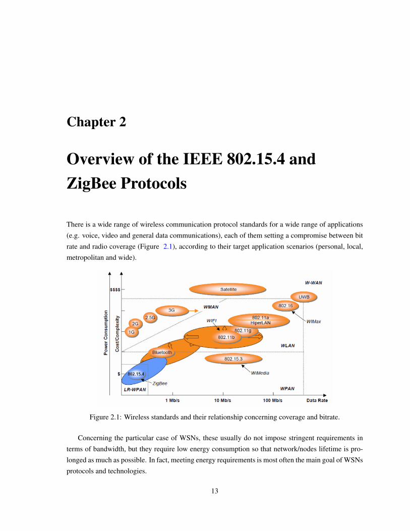
There is a wide range of wireless communication protocol standards for a wide range of applications
(e.g. voice, video and general data communications), each of them setting a compromise between bit
rate and radio coverage (Figure 2.1), according to their target application scenarios (personal, local,
metropolitan and wide).
Figure 2.1: Wireless standards and their relationship concerning coverage and bitrate.
Concerning the particular case of WSNs, these usually do not impose stringent requirements in
terms of bandwidth, but they require low energy consumption so that network/nodes lifetime is pro-
longed as much as possible. In fact, meeting energy requirements is most often the main goal of WSNs
protocols and technologies.
13

14 Overview of the IEEE 802.15.4 and ZigBee Protocols
Over the last decade a few standards aiming at low-power wireless communications have been
developed to cope with these requirements. A paradigmatic example is the IEEE 802.15.4 [IT06],
first published in 2003 for WPAN (Wireless Personal Area Networks). The protocol defines only the
physical and data-link layers, thus a few proposals such as the ZigBee [ZA05] or the RPL [WTB+12]
protocols followed to complement the stack.
However, to enable Cyber-Physical Systems (CPS) applications, besides the traditional WSNs re-
quirements, timeliness and predictability, among other aspects, must be also supported by the under-
lying communication layers. Nevertheless, there are a few limitations to the IEEE 802.15.4 standard,
some of those already identified in chapter 1 of this thesis, hence there is a need to consider new
mechanisms and add-ons. Devising these mechanisms is among the objectives of this thesis.
This chapter presents the most important features of the IEEE 802.15.4-2006 and ZigBee-2007
protocols. It particularly focuses on the IEEE 802.15.4 Data Link and ZigBee Network Layers, which
are the most relevant in the context of this thesis. The chapter ends with a birds eye view of other
competing protocols for WSNs.
2.1 The ZigBee Protocol
2.1.1 General Aspects
ZigBee defines two layers of the OSI (Open Systems Interconnection) model: the Application Layer
(APL) and the Network Layer (NWL), as depicted in Figure 2.2. Each layer provides a specific set of
services for the layer above. The different layers communicate through Service Access Points (SAP’s).
These SAPs enclose two types of entities: (1) a data entity (NLDE-SAP) to provide data transmission
service and (2) a management entity (NLME-SAP) providing all the management services between
layers.
The ZigBee Device Object (ZDO), located in EndPoint 0, is responsible for communicating in-
formation about its status and its provided services. The Application Objects consist of the set of
manufacturer’s applications running on top of the ZigBee protocol stack. These objects, located be-
tween Endpoints 1 to 240, adhere to a given profile approved by the ZigBee Alliance. The address
of the device and the EndPoints available provide a uniform way of addressing individual application
objects in the ZigBee network. The set of ZDOs, their configuration and functionalities form a ZigBee
profile. These ZigBee profiles intent to be a uniform representation of common application scenarios.
Currently, among the several ZigBee available profiles we can find the ZigBee Home Automation,
Smart Energy, Health Care, and Building Automation profiles.
The ZigBee Network Layer (NWK) is responsible for network management procedures (e.g.
nodes joining and leaving the network), security and routing. It also encloses the neighbour tables
and the storage of related information. It provides only one set of interfaces, the Network Layer

2.1 The ZigBee Protocol 15
Figure 2.2: ZigBee Architecture
Data Entity Service Access Point (NLDE-SAP) used to exchange data with the Application Sublayer
(APS).
IEEE 802.15.4/ZigBee devices can be classified according to their functionalities into two cate-
gories: Full Function Devices (FFD) implement the full IEEE 802.15.4/ZigBee protocol stack; Re-
duced Function Devices (RFD) implement a subset of the protocol stack. Regarding the devices role
in the network, ZigBee defines 3 types of devices:
– ZigBee Coordinator (ZC): One for each ZigBee Network; Initiates and configures Network for-
mation; Acts as an IEEE 802.15.4 Personal Area Network (PAN) Coordinator; Acts as a ZigBee
Router (ZR) once the network is formed; Is a Full Functional Device (FFD) – implements the
full protocol stack; If the network is operating in beacon-enabled mode, the ZC will send pe-
riodic beacon frames that will serve to synchronize the rest of the nodes. In a Cluster-Tree
network all ZR will receive beacon from their parents and send their own beacons to synchro-
nize nodes belonging to their clusters.
– ZigBee Router (ZR): Participates in multi-hop routing of messages in mesh and Cluster Tree

16 Overview of the IEEE 802.15.4 and ZigBee Protocols
networks; Associates with ZC or with previously associated ZR in Cluster-Tree topologies;
Acts as an IEEE 802.15.4 PAN Coordinator; It is a Full Functional Device (FFD) – implements
the full protocol stack.
– ZigBee End Device (ZED): Does not allow other devices to associate with it; Does not partici-
pate in routing; It is mostly a sensor/actuator node; Can be a Reduced Function Device (RFD)
– implementing a reduced subset of the protocol stack.
Throughout this thesis, the names of the devices and their acronyms are used interchangeably.
The ZigBee/IEEE 802.15.4 protocol enables three network topologies – star, mesh and cluster-tree
(Figure 2.3).
Figure 2.3: ZigBee Network Topologies
In the star topology (Figure 2.3 a), a unique node operates as a ZigBee Coordinator. The Zig-
Bee Coordinator chooses a PAN identifier, which must not be used by any other ZigBee network
in the vicinity. The communication paradigm of the star topology is centralized, i.e. each device
(FFD or RFD) joining the network and willing to communicate with other devices must send its data
to the ZigBee Coordinator, which dispatches it to the adequate destination. The star topology may
not be adequate for traditional Wireless Sensor Networks for two reasons. First, the sensor node se-
lected as a Coordinator will get its battery resources rapidly ruined. Second, the coverage of an IEEE
802.15.4/ZigBee cluster is very limited while addressing a large-scale WSN, leading to a scalability
problem.
The mesh topology (Figure 2.3 b) also includes a ZigBee Coordinator that identifies the entire
network. However, the communication paradigm in this topology is decentralized, i.e. each node can
directly communicate with any other node within its radio range. The mesh topology enables enhanced

2.1 The ZigBee Protocol 17
networking flexibility, but it induces additional complexity for providing end-to-end connectivity be-
tween all nodes in the network. Basically, the mesh topology operates in an ad-hoc fashion and allows
multiple hops to route data from any node to any other node. In contrast with the star topology, the
mesh topology may be more power-efficient and the battery resource usage is fairer, since the com-
munication process does not rely on one particular node.
The cluster-tree network topology (Figure 2.3 c) is a special case of a mesh network where there is
a single routing path between any pair of nodes and there is a distributed synchronization mechanism
supported by the IEEE 802.15.4 beacon-enabled mode. There is only one ZigBee Coordinator which
identifies the entire network and one ZigBee Router per cluster. Any of the FFD can act as a Router
providing synchronization services to other devices and ZigBee Routers.
2.1.2 The case for the Cluster-tree Topology
Table 2.1 summarizes some of the differences between ZigBee mesh and cluster-tree topologies.
Table 2.1: Comparison of network topologies
Star Mesh Cluster-Tree
Scalability No Yes YesSynchronization Yes No YesInactive Periods All nodes ZEDs All nodes
Guaranteed bandwidth Yes (GTS) No Yes (GTS)Redundant Paths N/A Yes No
Routing Protocol Overhead N/A Yes NoCommercially Available Yes Yes No
The synchronization (beacon-enabled mode) feature of the cluster-tree model may be seen both
as an advantage and as a disadvantage, as reasoned next. On the one hand, synchronization enables
dynamic duty-cycle management in a per cluster basis, allowing nodes (ZEDs and ZRs) to save their
energy by entering the sleep mode. In contrast, in the mesh topology as defined in the IEEE 802.15.4
standard specification, only the ZEDs can have inactive periods. These energy saving periods enable
the extension of the network lifetime, which is one of the most important requirements of WSNs.
In addition, synchronization allows the dynamic reservation of guaranteed bandwidth in a per-cluster
basis, through the allocation of Guaranteed Time Slots in the Superframe Contention Free Period
(CFP). This enables the worst-case dimensioning of cluster-tree ZigBee networks, namely it is possible
to compute worst-case message end-to-end delays and ZigBee Router buffer requirements.
On the other hand, managing the synchronization mechanism throughout the cluster-tree networks
is a very challenging task. Even if we can cope with minor synchronization drifts between ZRs, this
18 Overview of the IEEE 802.15.4 and ZigBee Protocols
problem can grow for larger cluster-tree networks (higher depths). As previously mentioned, the de-
synchronization of a cluster-tree network leads to collision problems due to overlapping Beacons and
Superframes. For instance, the CAP of one cluster can overlap the CFP of another cluster, which is
not admissible.
Regarding the routing protocols, the tree routing protocol in the cluster-tree is lighter that the mesh
routing protocol (AODV) in terms of memory and processing requirements. The routing overhead, as
compared with the AODV [IET03] in the mesh topology, is reduced. Note that the tree routing protocol
considers just one path from any source to any destination, thus it does not consider redundant paths, in
contrast to AODV. Therefore, the tree routing protocol is prone to the single point of failure problem,
while that can be avoided in mesh networks if alternative routing paths are available (more than one
ZigBee Router within radio coverage).
Note that if there is a fault in a ZigBee Router, network inaccessibility times may be inadmissible
for applications with critical timing and reliability requirements. Therefore, designing and engineering
energy and time-efficient fault-tolerance mechanisms to avoid or at least minimize the single point of
failure problem in ZigBee cluster-tree networks is of crucial importance.
Besides the Beacon/Superframe scheduling and the single-point-of-failure problems, there are
other implementation-related obstacles that makes the use of the cluster-tree topology a challenging
task, such as: (1) the dynamic network resynchronization, for instance in case of a new cluster joining
or leaving the network; (2) the dynamic rearrangement of the all the duty cycles in the case of a router
failure; (3) a new router association or even rearranging the superframe duration of some routers to
adapt the bandwidth allocated to that branch of the tree; (4) the rearrangement of the addressing space
allocated to each router; and (5) supporting mobility of nodes, routers or even hole clusters.
From our perspective, all these impairments have lead to the lack of commercial or academic
solutions based on the ZigBee cluster-tree model. Nevertheless, we consider this model as a promis-
ing and adequate solution for WSN applications with timeliness and energy-efficiency requirements,
which triggered us design new mechanisms to support this topology and to further explore its potential.
2.1.3 The ZigBee Network Layer
The ZigBee Network Layer is responsible for network management (e.g. association/disassociation,
starting the network, addressing, device configuration and the maintenance of the NIB - NWK Infor-
mation Base) and formation, message routing and security-related services. It provides two service
entities. The Network Layer Data Entity (NLDE) provides a data service, allowing the transmission
of data frames and topology specific routing. Figure 2.4 depicts the Network Layer reference model.
Joining and leaving a network must be supported by all ZigBee Devices. ZigBee Coordinators
and Routers must support additional functionalities such as permit devices to join the network using
Association indications from the MAC sub-layer or explicit join requests from the application; permit

2.1 The ZigBee Protocol 19
devices to leave the network using Network Leave command frames or via explicit leave requests
from the application. They must also participate in the assignment of logical network addresses and
maintain a list of neighbouring devices.
Figure 2.4: ZigBee Network Layer Reference Model
The ZigBee Coordinator also defines some important additional network parameters. It determines
the maximum number of children (Cm) any device is allowed to have. From this set of children, a
maximum number (Rm) of devices can be router-capable devices. The remaining are ZEDs. Every
device has an associated depth, representing the number of hops a transmitted frame must travel, using
only a parent-child links, to reach the ZigBee Coordinator. The ZigBee Coordinator has a depth of 0,
while its children have a depth of 1. It also determines the maximum depth (Lm) of the network. The
maximum number of children, routers and network depth are used for calculating the addresses of the
devices in the network, in a distributed address scheme.
2.1.3.1 Short Address Assignment
A parent device uses the Cm, Rm, and Lm values to compute a Cskip function defining the size of the
address sub-block that is distributed by each parent depending on its depth (d) in the network. For a
given network depth d, Cskip(d) is calculated as follows:
Cskip(d) =
1+Cm · (Lm−d−1) if Rm = 1,1+Cm−Rm−Cm·RmLm−d−1
1−Rm , otherwise(2.1)
A parent device that has a Cskip(d) value of zero is not capable of accepting children and must
be treated as an end device. A parent device that has a Cskip(d) value greater that zero must accept
devices and assigns addresses if possible. A parent device assigns an address that is greater than its
own to the first router that associated. The next associated router receives an address that is separated

20 Overview of the IEEE 802.15.4 and ZigBee Protocols
according to the return value of the Cskip(parentdepth) function. The maximum number of asso-
ciated routers is defined in the network parameter nwkMaxRouters(Rm). Considering a parent node
with a depth d and an address of Aparent , the number of child devices n is between 1 and Cm−Rm.
1≤ n≤ (Cm−Rm) (2.2)
The Achild address of the nth child router is calculated according to Eq. 2.3 (n is the number of
child routers):
Achild =
Aparent +(n−1) ·Cskip(d)+1, if n = 1
Aparent +(n−1) ·Cskip(d), n > 1(2.3)
The Achild address of the nth child end device is calculated according to Eq. 2.4 (n is the number
of child end devices):
Achild = Aparent +Rm ·Cskip(d)+n (2.4)
Figure 2.5 depicts an example of an address assignment scheme. The parameters used in the
address assignment are the following: maximum depth (Lm) = 3, maximum children (Cm) = 6 and
maximum routers (Rm) = 4.
Figure 2.5: ZigBee cluster-tree address assignment scheme example
Figure 2.6 shows the ZigBee Coordinator (0x0000) available addressing scheme. Considering the
above network parameters, the ZigBee Coordinator is allowed to associate up to 4 routers and 2 end
devices in its available address pool. On the other hand, the ZR (0x0020) is allowed to associate up to
4 ZRs and 6 ZEDs.

2.1 The ZigBee Protocol 21
Figure 2.6: ZigBee Coordinator addressing scheme example
2.1.3.2 ZigBee Routing
ZigBee Coordinators and Routers must provide a set of functionalities such as relaying data frames
on behalf of higher layers or other ZR; participate in route discovery in order to establish routes for
subsequent data frames or on behalf of end devices; and participate on route repairs.
Additionally, ZigBee Coordinators and Routers may provide functionalities such as maintaining
routing tables in order to remember best available routes; initiate route discovery on behalf of higher
layers or other ZR; carry out route repairs.
ZigBee Coordinators and Routers support three types of routing:
– Neighbour Routing – based on a neighbour tables that contains the information of all the devices
within radio coverage. If the target device is physically in range the message can be sent directly.
Note that ZEDs cannot do this.
– Table Routing - Ad-hoc On Demand Distance Vector (AODV) [IET03], based on routing and
route discovery tables with the path-cost metrics;
– Tree-Routing - based on the address assignment schemes; messages are hierarchically routed
upstream/downstream the tree.
Neighbour RoutingThis type of routing uses the neighbour tables. If the target device is physically in range it is possible
to send messages directly to the destination. Physically in range means that the source ZC or ZR has a
neighbour table entry for the destination. This routing mechanism is mostly used as addition to other
routing mechanisms and for the ZigBee Routers to route messages to its children devices, when they
are the destination.
Table Routing - Ad-hoc On-Demand Distance Vector (AODV)ZigBee Table Routing is based on the AODV routing algorithms. Each ZigBee Coordinator and
Router that supports this Table Routing must maintain two tables: (1) the routing table, a long-lived

22 Overview of the IEEE 802.15.4 and ZigBee Protocols
and persistent table with the information of routes, and (2) a route discovery table with the information
of the route discovery procedures where each entry only lasts the duration of the discovery.
The Ad-hoc On Demand Distance Vector routing protocol [IET03] was designed for ad hoc mo-
bile networks. AODV is capable of both unicast and multicast routing. AODV allows mobile nodes to
obtain routes quickly for new destinations, and does not require nodes to maintain routes to destina-
tions that are not in active communication, what allows mobile nodes to respond to link failures and
changes in network topology in a timely manner.
When the link breaks, AODV causes the affected set of nodes to be notified so that they are able
to invalidate the routes using the lost link. It is an on demand algorithm, meaning that it builds routes
between nodes only if requested by source nodes. It maintains these routes as long as they are needed
by the sources.
Routing management is done by the means of NWK command frames. To carry out this task,
ZigBee supports the following commands:
– Route request – Command send to search for a route to a specified device, can also be used to
repair a route;
– Route reply – Command send in response of a route request, also used to request state informa-
tion;
– Route Error – notification of a source device of the data frame about the failure in forwarding
the frame;
– Leave – notification of a device leaving the network;
– Route Record – notification of a list of nodes used in relaying a data frame;
– Rejoin request – notification of a device rejoining the network;
– Rejoin response – rejoin response of a rejoin request;
The route choice for a communication flow is based on the total link cost represented by C, mean-
ing that the path with the lowest cost is chosen. The total link cost is the sum of individual point-to-
point link cost. The calculation of C is as follows: for a defined path P where L defines the number of
a set of devices [D1,D2, . . .DL] and a link [Di,Di+1] the path cost C is defined as:
C{P}=L−1
∑i=1
C{[D1,Di+1]} (2.5)
Each C[D1,Di+1] is the individual point-to-point link cost, calculated by the following formula-
tion:
C{l}=
7,
min(
7, round(
1p4
l
)) (2.6)
where pl is defined as the probability of packet delivery through link l.

2.1 The ZigBee Protocol 23
The link probability estimation factors are implementation specific, but generally it they are based
on the counting of the received beacons and data frames in order to detect packet loss and in the
estimation of the Link Quality Indicator (LQI).
Tree-RoutingThis routing mechanism is based on the short addressing scheme and was initially proposed by MO-
TOROLA. Each device, upon the reception of a data frame, reads the routing information fields and
checks the destination address. If the destination is a child of the device (neighbour table check),
the device relays the packet to the appropriate address. If the destination address is not a child, the
device must check if the address is a descendent using the condition in 2.7, where A is device network
address, D the destination address and d the device depth in the network.
A < D < A+Cskip(d−1) (2.7)
The next hop (N) address when routing down is given by:
N = A+1+⌊
D− (A+1)Cskip(d)
⌋Cskip(d) (2.8)
If the destination address is not a descendant, the device relays the packet to its parent.
Consider the network scenario illustrated in Figure 2.5 and the following network parameters:
Lm = 3; Cm = 6; Rm = 4. The Cskip values are presented in Table 2.2.
Table 2.2: Cskip example values
depth Cskip(depth)
0 311 72 1
If ZR 0x0002 transmits a message to ZR 0x0028, the tree-routing protocol behaves as follows:
1. ZR 0x0002 builds the data frame and sends it to its parent (0x0001). The most relevant fields of
this data frame are outlined next:
– MAC destination address – 0x0001;
– MAC source address – 0x0002;
– Network Layer Routing Destination Address – 0x0028;
– Network Layer Routing Source Address – 0x0002;

24 Overview of the IEEE 802.15.4 and ZigBee Protocols
2. ZR 0x0001 receives the data frame, realizes that the message in not for him and has to be re-
layed. The device checks its neighbour table for the routing destination address, trying to find if the
destination is one of its child devices. Then, the device checks if the routing destination address is a
descendant by verifying condition in Eq. 2.7 that results in:
0x0001 < 0x0028 < 0x0001+7 (2.9)
Note that ZR 0x0001 is a depth 1 device in the network. After verifying that the destination is not
a descendant, ZR 0x0001 routes the data frame to its parent, ZC 0x0000. The most relevant fields of
this data frame are outlined next:
– MAC destination address – 0x0000;
– MAC source address – 0x0001;
– Network Layer Routing Destination Address – 0x0028;
– Network Layer Routing Source Address – 0x0002;
3. ZC 0x0000 receives the data frame and verifies if the routing destination address exists in its
neighbour table. After realizing that the destination device is not its neighbour, since the ZC is the
root of the tree and cannot route up, the next hop address is calculated as follows:
N = 0x0000+1+⌊
0x0028− (0x0000+1)31
⌋×31 (2.10)
The next hop address results in N = 32 (decimal) = 0x0020. The most relevant fields of this data
frame are outlined next:
– MAC destination address – 0x0020;
– MAC source address – 0x0000;
– Network Layer Routing Destination Address – 0x0028;
– Network Layer Routing Source Address – 0x0002;
4. ZR 0x0020 receives the data frame and checks its neighbour table for the routing destination
address. After verifying that the address is its neighbour, the message is routed to it. The next hop
is assigned with the short address present in the respective neighbour table entry. The most relevant
fields of this data frame are outlined next:
– MAC destination address – 0x0028;
– MAC source address – 0x0020;
– Network Layer Routing Destination Address – 0x0028;
– Network Layer Routing Source Address – 0x0002;

2.1 The ZigBee Protocol 25
Figure 2.7: Time division approach to the beacon scheduling problem
2.1.3.3 Beacon Scheduling
Although the cluster-tree network concept is outlined in the ZigBee specification, there is not a clear
description on how this model can be implemented. The available information regarding this topology
consists in a broad overview on how the cluster-tree network should operate and some details on the
tree-routing algorithm.
However, there are a few issues which must be addressed to engineer these networks. In particular,
the cluster-tree model includes more than one ZigBee Router that periodically generates beacons to
synchronize nodes (or clusters of nodes) in their neighbourhood. If these periodic beacon frames
are sent in an unplanned fashion, without any particular schedule, they will collide with each other
or with other frames. These collisions will result in the loss of synchronization between a parent
ZigBee Router and their child devices, which prevents them to communicate. Therefore, beacon
frame scheduling mechanisms must be defined to avoid beacon frame collisions in ZigBee cluster-tree
networks.
To address this, the Task Group 15.4b working in an improved version of the IEEE 802.15.4
standard, proposed a couple of approaches to avoid beacon frame collisions. A first approach, called
the beacon-only period approach, consisted in a time window at the beginning of each superframe
reserved for beacon frame transmissions only. The second approach, based on time division, proposed
that beacon frames of a given cluster were sent during the inactivity periods of the other clusters.
However, these proposals did not define how to schedule beacon frame transmissions, specially how
to choose the time offsets of the different beacons. Surprisingly, these approaches, discussed within
the Task Group 15.4b, were not fully included in the subsequent versions of the standards.
The beacon only period proposed by Task Group 15.4b imposes major changes in the protocol,
does not allow GTS allocations and it needs a complex scheduling mechanism. Another problem of
the beacon only period is how to define the beacon transmission window size that can lead to scale
limitations of this approach. In this line, the time-division approach appears as a more appealing
solution.
In this approach, time is divided such that beacon frames and the superframe duration of a given
Coordinator are scheduled in the inactive period of its neighbour Coordinators, as shown in Figure 2.7.

26 Overview of the IEEE 802.15.4 and ZigBee Protocols
Each Coordinator uses a starting time relative to the Coordinator beacon ( Beacon_Tx_Offset) to trans-
mit its beacon frames. The beacon offsets must be different for each router so that each active period
uses a different time window. This approach requires that a Coordinator wakes up both in its active
period and in its parent’s active period to track its beacon. Communication between different clusters
must be accomplished by the means of indirect transmissions. Observe that Beacon_Tx_Offset must
be chosen adequately, not only to avoid beacon frame collisions, but also to enable efficient utilization
of inactive periods, thus maximizing the number of clusters in the same network.
To engineer these networks and effectively schedule the active portions of the different clusters,
[KCAT08] proposed the Time Division Beacon Scheduling (TDBS) mechanism, which was also im-
plemented in TinyOS and made available via the Open-ZB website ([OZ15]). It is also available within
the TinyOS repositories, as part of the ZigBee WG ([Tind]) contributions.
The implementation of this mechanism assumes the following:
1. The ZigBee Network Layer supports the tree-routing mechanism, thus the network addresses of
the devices are assigned accordingly;
2. The ZigBee Coordinator is the first node broadcasting beacons in the network;
3. The ZigBee Routers start to send beacons only after a successful negotiation.
4. The same Beacon Interval (BI) is used by every ZigBee Router. Note that this just a simple
choice to simply the implementation, without loss of generality. This would also be feasible for
the case of different BIs, but with a slightly higher implementation complexity;
The TDBS approach relies on a negotiation prior to beacon transmission. Upon success of the
association to the network, a ZR (initially behaving as a ZED) sends a negotiation message to the ZC
(routed along the tree) embedding the envisaged (BO, SO) pair, requesting a beacon broadcast permit.
Then, in the case of a successfully negotiation, the ZC replies with a negotiation response message
containing a beacon transmission offset (the instant when the ZR must start transmitting the beacon).
In case of rejection, the ZR must disassociate from the network.
Figure 2.8 depicts the architecture of the TDBS implementation in the IEEE 802.15.4/ZigBee
protocol stack. The Admission Control and Scheduling algorithm fits as a service module of the
Application Support Layer. The TDBS requires minor changes to the Network Layer. It is necessary to
add a StartTime argument to the MLME-START.request primitive, as already proposed in the ZigBee
Specification, and to the NLME-START-ROUTER.request primitive. The StartTime parameter will be
used as a transmission offset referring to the parent ZigBee Router (ZR). In the ZC, the value of this
parameter is 0.
After a successful negotiation of the beacon transmission, the ZR will have two active periods: its
own (the superframe duration) and its parent’s superframe duration. In its own active period, the ZR
is allowed to transmit frames to its child nodes or relay frames to the descendant devices in the tree.
The frames destined upstream are sent during its parent’s active period.

2.2 Overview of the IEEE 802.15.4 Protocol 27
Figure 2.8: TDBS implementation in the IEEE 802.15.4 stack
2.2 Overview of the IEEE 802.15.4 Protocol
In the IEEE 802.15.4-2006 version of the standard, the Full Function Devices (FFD) have three dif-
ferent operation modes:
– The Personal Area Network (PAN) Coordinator: the principal controller of the PAN. This de-
vice identifies its own network as well as its configurations, to which other devices may be
associated. In ZigBee, this device is referred to as the ZigBee Coordinator (ZC).
– The Coordinator: provides synchronization services through the transmission of beacons. This
device should be associated to a PAN Coordinator and does not create its own network. In
ZigBee, this device is referred to as the ZigBee Router (ZR).
– The End Device: a device which does not implement the previous functionalities and should
associate with a ZC or ZR before interacting with the network. In ZigBee, this device is referred
to as the ZigBee End Device (ZED).
The Reduced Function Device (RFD) is an end device operating with the minimal implementation
of the IEEE 802.15.4. An RFD is intended for applications that are extremely simple, such as a light
switch or a passive infrared sensor; they do not have the need to send large amounts of data and may

28 Overview of the IEEE 802.15.4 and ZigBee Protocols
Figure 2.9: Operating frequencies and bands
only associate with a single FFD at a time. Throughout this thesis the IEEE 802.14.5 operational
modes and the ZigBee device names are used interchangeably (e.g. PAN Coordinator = ZigBee Co-
ordinator, Coordinator = ZigBee Router and End Device = ZigBee End Device). The designation of
Coordinator represents both ZC and ZRs.
2.2.1 Physical Layer
The IEEE 802.15.4 physical layer is responsible for data transmission and reception using a certain
radio channel and according to a specific modulation and spreading technique. The IEEE 802.15.4
offers three operational frequency bands: 2.4 GHz, 915 MHz and 868 MHz (Figure 2.9). There is a
single channel between 868 and 868.6 MHz (20 kbit/s), 10 channels between 902 and 928 MHz (40
kbit/s), and 16 channels between 2.4 and 2.4835 GHz (250 kbit/s). The protocol also allows dynamic
channel selection, a channel scan function in search of a beacon, receiver energy detection, link quality
indication and channel switching.
All of these frequency bands are based on the Direct Sequence Spread Spectrum (DSSS) spreading
technique. The physical layer of IEEE 802.15.4 is in charge of the following tasks:
– Activation and deactivation of the radio transceiver: The radio transceiver may operate in one
of three states: transmitting, receiving or sleeping. Upon request of the MAC sub-layer, the
radio is turned ON or OFF. The turnaround time from transmitting to receiving and vice versa
should be no more than 12 symbol periods, according to the standard (each symbol corresponds
to 4 bits).

2.2 Overview of the IEEE 802.15.4 Protocol 29
– Energy Detection (ED): Estimation of the received signal power within the bandwidth of an
IEEE 802.15.4 channel. This task does not make any signal identification or decoding on the
channel. The energy detection time should be equal to 8 symbol periods. This measurement is
typically used by the Network Layer as a part of channel selection algorithm or for the purpose
of Clear Channel Assessment (CCA), to determine if the channel is busy or idle.
– Link Quality Indication (LQI): Measurement of the Strength/Quality of a received packet. It
measures the quality of a received signal. This measurement may be implemented using receiver
ED, a signal to noise estimation or a combination of both techniques.
– Clear Channel Assessment (CCA): Evaluation of the medium activity state: busy or idle. The
CCA is performed in three operational modes: (1) Energy Detection mode: the CCA reports
a busy medium if the detected energy is above the ED threshold. (2) Carrier Sense mode: the
CCA reports a busy medium only is it detects a signal with the modulation and the spreading
characteristics of IEEE 802.15.4 and which may be higher or lower than the ED threshold. (3)
Carrier Sense with Energy Detection mode: this is a combination of the aforementioned tech-
niques. The CCA reports that the medium is busy only if it detects a signal with the modulation
and the spreading characteristics of IEEE 802.15.4 and with energy above the ED threshold.
– Channel Frequency Selection: The IEEE 802.15.4 defines 27 different wireless channels. Each
network can support only part of the channel set. Hence, the physical layer should be able to
tune its transceiver into a specific channel when requested by a higher layer.
2.2.2 Medium Access Control (MAC) Sub-layer
The IEEE 802.15.4-2006 protocol supports two operational modes (Figure 2.10):
Figure 2.10: IEEE 802.15.4 operational modes

30 Overview of the IEEE 802.15.4 and ZigBee Protocols
Figure 2.11: IEEE 802.15.4 superframe structure
– The non beacon-enabled mode: When the ZC selects the non-beacon enabled mode, there are
neither beacons nor superframes. Medium access is ruled by an unslotted CSMA/CA mecha-
nism (refer to Section 2.2.6).
– The beacon-enabled mode: In this mode, beacons are periodically sent by the ZC or ZR to
synchronize nodes that are associated with it, and to identify the PAN. A beacon frame delim-
its the beginning of a superframe defining a time interval during which frames are exchanged
between different nodes in the PAN. Medium access is basically ruled by Slotted CSMA/CA.
However, the beacon-enabled mode also enables the allocation of contention free time slots,
called Guaranteed Time Slots (GTSs) for nodes requiring guaranteed bandwidth.
Superframe StructureThe superframe is defined between two beacon frames and has an active period and an inactive period.
Figure 2.11 depicts the IEEE 802.15.4 superframe structure.
The active portion of the superframe structure is composed of three parts, the Beacon, the Con-
tention Access Period (CAP) and the Contention Free Period (CFP):
– Beacon: the beacon frame is transmitted at the start of slot 0. It contains the information on the
addressing fields, the superframe specification, the GTS fields, the pending address fields and
other PAN related information.
– Contention Access Period (CAP): the CAP starts immediately after the beacon frame and ends
before the beginning of the CFP, if it exists. Otherwise, the CAP ends at the end of the active
part of the superframe. The minimum length of the CAP is fixed at aMinCAPLength = 440
symbols. This minimum length ensures that MAC commands can still be transmitted when
GTSs are being used. A temporary violation of this minimum may be allowed if additional
space is needed to temporarily accommodate an increase in the beacon frame length, needed

2.2 Overview of the IEEE 802.15.4 Protocol 31
to perform GTS management. All transmissions during the CAP are made using the Slotted
CSMA/CA mechanism. However, the acknowledgement frames and any data that immediately
follows the acknowledgement of a data request command are transmitted without contention. If
a transmission cannot be completed before the end of the CAP, it must be deferred until the next
superframe.
– Contention Free Period (CFP): The CFP starts immediately after the end of the CAP and must
complete before the start of the next beacon frame (if BO equals SO) or the end of the super-
frame. Transmissions are contention-free since they use reserved time slots (GTS) that must be
previously allocated by the ZC or ZR of each cluster. All the GTSs that may be allocated by the
Coordinator are located in the CFP and must occupy contiguous slots. The CFP may therefore
grow or shrink depending on the total length of all GTSs.
In beacon-enabled mode, each Coordinator defines a superframe structure Figure 8 which is con-
structed based on the Beacon Interval (BI), which defines the time between two consecutive beacon
frames and the Superframe Duration (SD), which defines the active portion in the BI, and is divided
into 16 equally-sized time slots, during which frame transmissions are allowed.
Optionally, an inactive period is defined if BI > SD. During the inactive period (if it exists), all
nodes may enter in a sleep mode (to save energy). BI and SD are determined by two parameters, the
Beacon Order (BO) and the Superframe Order (SO), respectively, as follows:
BI = aBaseSuper f rameDuration×2BO
SD = aBaseSuper f rameDuration×2SO
}for 0≤ SO≤ BO≤ 14 (2.11)
aBaseSuper f rameDuration = 15.36 ms (assuming 250 kbps in the 2.4 GHz frequency band) de-
notes the minimum duration of the superframe, corresponding to SO=0. As depicted in Figure 8,
low duty cycles can be configured by setting small values of the SO as compared to BO, resulting
in greater sleep (inactive) periods. In ZigBee Cluster-Tree networks, each cluster can have different
and dynamically adaptable duty-cycles. This feature is particularly interesting for WSN applications,
where energy consumption and network lifetime are main concerns. Additionally, the Guaranteed
Time Slot (GTS) mechanism is quite attractive for time-sensitive WSNs, since it is possible to guar-
antee end-to-end message delay bounds both in Star and Cluster-Tree topologies.
Association and Channel Scan MechanismsThe association procedure takes place when a device wants to associate with a Coordinator. This
mechanism can be divided into three separate phases: (1) channel scan procedure; (2) selection of a
possible parent; (3) association with the parent.
IEEE 802.15.4 enables four types of channel scan procedures: (1) the energy detection scan,
where the device obtains a measure of the peak energy in each channel; (2) the active scan, where the

32 Overview of the IEEE 802.15.4 and ZigBee Protocols
device locates all Coordinators transmitting beacon frames; this scan is performed on each channel
by first transmitting a beacon request command; (3) the passive scan, where similarly to the active
scan, the device locates all Coordinator transmitting beacon frames with the difference that the scan
is performed only in a receive mode, without transmitting beacon requests; and (4) the orphan scan,
used to locate the Coordinator with which the scanning device had previously associated.
After the channel scan procedure is completed, the NWK layer receives a list of all detected PAN
descriptors (containing information about the potential parents). Based on the information collected
during the scan, the device can choose the most suitable parent (that permits associations).
For a device to associate to a Coordinator, it must send an association command frame. Then, if
the Coordinator accepts the device, it adds it to its neighbour table as its child. An association re-
sponse command frame is, in the case of a successful association, sent to the device (via an indirect
transmission), embedding its short address. Otherwise, in the case of an unsuccessful association,
the association response embeds the problem status information. The Coordinator replies to the as-
sociation command frame with an acknowledgement embedding the pending data control flag active,
meaning that it has data ready to be transmitted to the device. The association procedure is completed
when the device sends a data request command frame to the Coordinator requesting the pending data
(the association response command). After a successful association, the device stores all the infor-
mation about the new PAN by updating its MAC PAN Information Base (MAC PIB) and can start
transmissions. Figure 2.12 exemplifies the sequence of messages for a successful association request,
followed by a data transmission.
Figure 2.12: Association mechanism example

2.2 Overview of the IEEE 802.15.4 Protocol 33
Figure 2.13: Disassociation mechanism example
The disassociation from a Coordinator is done via a disassociation request command. The disasso-
ciation can be initiated either by the device or by the Coordinator. After the disassociation procedure,
the device loses its short address and is not able to communicate.
The Coordinator updates the list of associated devices, but it can still keep the device information
for a future re-association. Figure 2.13 shows a transmission sequence of a disassociation request
initiated by a device.
Figure 2.14: GTS allocation message diagram
Guaranteed Time Slot (GTS) mechanismThe GTS mechanism allows devices to access the medium without contention, in the CFP. GTSs are
allocated by the Coordinator and are used only for communications between the Coordinator and a
device. Each GTS may contain one or more time slots. The Coordinator may allocate up to seven
GTSs in the same superframe, provided that there is sufficient capacity in the superframe. Each GTS
has only one direction: from the device to the Coordinator (transmit) or from the Coordinator to the
device (receive). Figure 2.14 illustrates message sequence diagram for a GTS allocation.

34 Overview of the IEEE 802.15.4 and ZigBee Protocols
The GTS can be deallocated at any time at the discretion of the Coordinator or the device that
originally requested the GTS allocation. A device to which a GTS has been allocated can also transmit
during the CAP. The Coordinator is responsible for performing the GTS management; for each GTS,
it stores the starting slot, length, direction, and associated device address. All these parameters are
embedded in the GTS request command. Only one transmit and/or one receive GTS are allowed
for each device. Upon the reception of the deallocation request the Coordinator updates the GTS
descriptor list by removing the previous allocated slot and rearranging the remaining allocation starting
slots. The arrangement of the CFP consists in shifting right the allocated GTS descriptors with starting
slot before the recent deallocated GTS descriptor and consequently the final CAP slot variable is
updated. Figure 2.15 illustrates an example of this procedure.
Figure 2.15: CFP defragmentation upon GTS deallocation
In Figure 2.15, the 1st timeline represents the three allocated GTS. The 2nd timeline shows the
deallocation of GTS 2 that starts on the 10th time slot and has duration of 4 time slots. The final
timeline show GTS 3 shifted right by 4 time slots. The first CTF time slot shifted right from slot 8 (in
timeline 1) to slot 12 (in timeline 3).
The Coordinators monitors GTS activity and if there are no transmissions during a defined number
of time slots the GTS allocation expires. The expiration occurs if no data or no acknowledgement

2.2 Overview of the IEEE 802.15.4 Protocol 35
frames are received by the device or by the Coordinator, on every 2∗n superframes, where n is defined
as: {n = 28−macBeaconOrder, if 0≤ macBeaconOrder ≤ 14
n = 1, if 9≤ macBeaconOrder ≤ 14(2.12)
CSMA/CA MechanismIn IEEE 802.15.4, contention-based MAC (Medium Access Control) can be either slotted or unslotted
CSMA/CA, depending on the network operation behaviour: beacon-enabled or non beacon-enabled
modes, respectively.
The CSMA/CA mechanism is based on backoff periods (with the duration of 20 symbols). Three
variables are used to schedule medium access:
– Number of Backoffs (NB), representing the number of failed attempts to access the medium;
– Contention Window (CW ), representing the number of backoff periods that must be clear before
starting transmission;
– Backoff Exponent (BE), enabling the computation of the number of wait backoffs before at-
tempting to access the medium again.
Figure 2.16 depicts a flowchart describing the slotted version of the CSMA/CA mechanism. It can
be summarized in five steps:
1. Initialization of the algorithm variables: NB equal to 0; CW equals to 2 and BE is set to the
minimum value between 2 and a MAC sub-layer constant (macMinBE = 3);
2. After locating a backoff boundary, the algorithm waits for a random defined number of backoff
periods before attempting to access the medium;
3. Clear Channel Assessment (CCA) to verify if the medium is idle or not.
4. The CCA returned a busy channel, thus NB is incremented by 1 and the algorithm must start
again in Step 2;
5. The CCA returned an idle channel, CW is decremented by 1 and when it reaches 0 the message
is transmitted, otherwise the algorithm jumps to Step 3.
In the slotted CSMA/CA, when the battery life extension is set to 0, the CSMA/CA must ensure
that, after the random backoff (step 2), the remaining operations can be undertaken and the frame
can be transmitted before the end of the CAP. If the number of backoff periods is greater than the
remaining in the CAP, the MAC sub-layer pause the backoff countdown at the end of the CAP and
defers it to the start of the next superframe. If the number of backoff periods is less or equal than the
remaining number of backoff periods in the CAP, the MAC sub-layer applies the backoff delay and

36 Overview of the IEEE 802.15.4 and ZigBee Protocols
Figure 2.16: The slotted CSMA/CA mechanism
re-evaluate whether it can proceed with the frame transmission. If the MAC sub-layer do not have
enough time, it defers until the start of the next superframe, continuing with the two CCA evaluations
(step 3). If the battery life extension set to 1, the backoff countdown must only occur during the first
six full backoff periods, after the reception of the beacon, as the frame transmission must start in one
of these backoff periods.
Figure 2.17: The unslotted CSMA/CA mechanism
The non slotted mode of the CSMA/CA (Figure 2.17) is very similar to the slotted version except
the algorithm does not need to rerun (CW number of times) when the channel is idle.

2.2 Overview of the IEEE 802.15.4 Protocol 37
Transmission scenarios and reception conditions
The IEEE 802.15.4 protocol standard enables three different types of transmissions:
1. Direct transmissions – the frames are transmitted to the medium without any channel assessment
i.e. the beacon frames, the acknowledgment frames and the frames in the GTS time slots;
2. Indirect transmissions – the frames are stored in the Coordinator to which the destination device
is associated. Then, the information about the stored frames (or pending transmissions) is in-
cluded in the pending addresses descriptors fields of the beacon frame. If a device has pending
data in the Coordinator it can request it by sending a data request command frame. An exam-
ple of this mechanism is depicted in Figure 2.18 where the Coordinator beacon contains the
short address 0x0004 in the pending address list. In the Coordinator neighbour table, the short
address 0x0004 is associated to the extended address 0x0000000400000004. Then, the device
0x0004 requests the data with a data request message embedding its extended address. The
Coordinator searches in its neighbour tables for the short address corresponding to the extended
address received in the command frame and transmit the corresponding pending data. In the
next Coordinator beacon the pending address list is updated.
3. Normal transmissions – the frames are transmitted to the medium with contention, by applying
the CSMA/CA algorithm i.e. data frames and command frames transmitted during the CAP.
Depending of the operation mode (beacon-enabled or non beacon-enabled) the CSMA/CA al-
gorithm has two versions, the slotted or the unslotted respectively.
Figure 2.18: Indirect transmission example
Three different transmissions scenarios are possible during the CAP:
– Successful data transmission – the sender successfully transmits the frame to the intended recip-
ient. The recipient receives the frame and sends an acknowledgment if required. If it is an ac-
knowledged request, the sender starts a timer that expires after macAckWaitDuration symbols.

38 Overview of the IEEE 802.15.4 and ZigBee Protocols
Upon the reception of the acknowledge frame (before the timer expires), the sender disables and
reset the timer. The data transfer is completed successfully.
– Loss of frame – the sender successfully transmits the frame to the medium but it never reaches
the destination, so that an acknowledgement frame is not transmitted. The sender timer expires
(after macAckWaitDuration) and the sender retransmits the frame again. This procedure is
repeated up to a maximum of aMaxFrameRetries times after which the transmission aborts.
– Loss of acknowledgement - the sender successfully transmits the frame to the intended recipient
that upon reception replies with an acknowledgement frame. The sender never receives the
acknowledgement and retries the transmission.
Concerning reception conditions, the MAC sub-layer will only accepts frames from the Phy layer
if they satisfy the following requirements:
– The frame type subfield of the frame control field does not contain an illegal frame type;
– If the frame type indicates that the frame is a beacon frame, the source PAN identifier must
match macPANId, unless macPANId is equal to 0xffff, in which case the beacon frame must be
accepted regardless of the source PAN identifier;
– If a destination PAN identifier is included in the frame, it must match macPANId or the broad-
cast PAN identifier (0xffff);
– If a short destination address is included in the frame, it must match either macShortAddress or
the broadcast address (0xffff). Otherwise, if an extended destination address is included in the
frame, it must match aExtendedAddress;
– If only source addressing fields are included in a data or MAC command frame, the frame is
accepted only if the device is a Coordinator and the source PAN identifier matches macPANId.
Inter-Frame Spacing (IFS)
The inter-frame spacing (IFS) is an idle communication period that is needed for supporting the
MAC sub-layer needs to process data received by the physical layer. To allow this, all transmitted
frames are followed by an IFS period. If the transmission requires an acknowledgment, the IFS will
follow the acknowledgement frame. The length of the IFS period depends on the size of the transmitted
frame: a long inter-frame spacing (LIFS) or short inter-frame spacing (SIFS). The selection of the IFS
is based on the IEEE 802.15.4 aMaxSIFSFrameSize parameter, defining the maximum allowed frame
size to use the SIFS. The CSMA/CA algorithm takes the IFS value into account for transmissions in
the CAP. These concepts are illustrated in Figure 2.19.

2.3 A Review of Other Standard Protocols for WSNs 39
Figure 2.19: Inter-frame spacing
2.3 A Review of Other Standard Protocols for WSNs
To complement the IEEE 802.15.4 standard and achieve a higher integration with the Internet, var-
ious IETF working groups have made several proposals such as the IPv6 over Low power WPAN
(6LoWPAN), Routing Over Low power and Lossy networks (ROLL) and IETF Constrained RESTful
Environments (CORE). At the network layer, the IETF 6LoWPAN working group has started in 2007
to specify a protocol, 6LoWPAN [6Lo15], for transmitting IPv6 over IEEE 802.15.4 networks by
introducing 6LoWPAN adaptation layer. On top of that, the IETF ROLL working group has standard-
ized a Routing Protocol for Low Power and Lossy Networks (RPL) [WTB+12]. At the application
layer, a Constrained Application Protocol (CoAP) has been defined by the IETF CORE working group
with the purpose of running RESTful architectures such as the client/server model defined by Hyper-
Text Transfer Protocol (HTTP) over low-power and constrained wireless networks, meeting very low
overhead and simplicity for constrained environments.
However, although these proposals may be suitable for applications in the Internet domain, other
applications in areas such as the process industry, present different requirements, some of those shared
with Cyber Physical Systems (CPS). The IEEE 802.15.4 protocol presents several issues such as reli-
ability due to radio interferences and the high energy consumption under higher traffic loads, mostly
caused by channel access inefficiency. To tackle this, other proposals have been put forward, such
as the IEEE 802.15.4e [IEE15a] standard, WirelessHART [ Wi10], ISA 100.11a [ISA09], WIA-PA
[WIA11] or DASH7 [DAS13], specially targeting the process industry.
WirelessHART (IEC 62591)
Officially presented by the HART Communication Foundation in September, 2007, WirelessHART
was the first open standard specifically designed for wireless communication in process measurement

40 Overview of the IEEE 802.15.4 and ZigBee Protocols
and control applications. Its aim was to be compatible with existing HART devices by adding wireless
communication capability to the HART protocol. At the very bottom of its stack, it adopts IEEE
802.15.4-2006 as the physical layer. On top of that, WirelessHART defines its own time-synchronized
MAC layer featuring a TDMA access mechanism combined with channel hopping. The regular IEEE
802.15.4 superframe is not supported by WirelessHART. Its superframe consists of multiple time-slots,
in which a packet transaction can take place.
WirelessHART network layer supports self-organizing and self-healing mesh networking tech-
niques. In this way, messages can be routed around interferences and obstacles. It adopts a centralized
routing scheme, in which the network manager is responsible for maintaining up-to-date routes and
communication schedules for devices in the network. A channel blacklisting feature is also provided
to restrict the number of hopping sequences. Each link containing a transmitter and a receiver is as-
signed to the channel hopping sequence and switch the channel after a transaction. WirelessHART
specification was approved by IEC as a full international standard (IEC 62591) in March 2010.
ISA-100.11a (IEC 62734)
ISA-100.11a describes a mesh network designed to provide secure wireless communication to process
control. It’s MAC employs the same superframe structure as WirelessHART. In addition, it supports
three channel hopping operating modes: slotted channel hopping, slow channel hopping and hybrid
combinations of slotted and slow hopping. Just like WirelessHART, a centralized network manager is
responsible to generate a hopping pattern. In slotted channel hopping mode, a time slot in a superframe
is assigned a dedicated channel and the next time slot shall use the next successive channel in the
hopping pattern. The hopping pattern is repeatable as time progresses. For a given hopping pattern, the
standard provides a mapping between channel number in hopping pattern and MAC channel numbers.
In slow hopping mode, multiple consecutive time slots are assigned a common channel. This
method supports devices with imprecise timing settings. The slow hopping also serves as a way to
improve support for event-based traffic. Usually a group of devices share a slow hopping period in a
contention-based way, that is, transmissions in a slow hopping period is CSMA/CA based. When an
event triggers the need for a device to immediately transmit a data packet or an alarm, the device does
not need to wait for the next time slot that is assigned to it, thereby reducing the latency. However,
slow hopping increasing devices’ energy consumption as they have to listen to the channel for possible
incoming packets.
In general, ISA-100.11a is more flexible by providing more configurable parameters than Wire-
lessHART. For example, the time slot size is fixed at 10ms in WirelessHART while in ISA100.11a it is
configurable on a per-superframe base. Both standards use Time Division Multiple Access (TDMA)
with frequency hopping for channel access in the 2.4 GHz band. The combination of direct sequence
spread spectrum (DSSS) and frequency-hopping spread spectrum (FHSS) makes WirelessHART and
ISA-100.11a more robust to interference in harsh industrial environments.

2.3 A Review of Other Standard Protocols for WSNs 41
WIA-PA (IEC 62601)
The Chinese Industrial Wireless Alliance was established in 2007 aiming to develop standards for
industrial wireless network [LLYL13]. Wireless network for Industrial Automation - Process Au-
tomation (WIA-PA) is the first standard developed by the alliance for process industries, and defines
the system architecture and communication specifications. It was approved by IEC as international
standard (IEC 62601) in 2011.
The WIA-PA MAC has a compatible IEEE 802.15.4 superframe structure with redefined functions
for CAP, CFP and inactive period. The CAP is used for packet transmission of device joining, intra-
cluster management and retransmissions. The access method in the CAP is CSMA/CA mechanism
defined in IEEE 802.15.4, which is different from WirelessHART and ISA-100.11a. Each WIA-PA
time slot duration in CFP is configurable and compatible with IEEE 802.15.4 GTS. Except the sleep
mode, intra- and inter-cluster communication is allowed during the inactive period. WIA-PA supports
three channel hopping mechanisms: adaptive frequency switch (AFS), adaptive frequency hopping
(AFH), time slot hopping (TH) in which the channel is changed per time slot. The channel hopping
sequence is determined by the network manager.
At the network layer, all of the standards overview so far support a mesh network architecture with
different routing protocols to overcome obstacles, reach longer distances, and create resilient paths for
increasing reliability. However, WirelessHART and WIA-PA do not support the IPv6 packet format,
while ISA-100.11a does, by employing the IETF 6LoWPAN protocol as an adaptation sublayer.
Concerning the transport layer, WIA-PA does not specify any protocols, while ISA-100.11a uses
User Datagram Protocol (UDP) and WirelessHART utilizes its own proprietary protocol. At the ap-
plication layer, a HART-compliant protocol is used in WirelessHART to be compliant with existing
HART devices. WIA-PA uses a proprietary protocol while ISA-100.11a does not specify any protocols
in this layer.
IEEE 802.15.4e
The IEEE802.15.4e standard released in 2012 defines a MAC amendment to the existing standard
IEEE 802.15.4-2006 to better support industrial markets. It aims to achieve better reliability and
lower power consumption through time-synchronized channel hopping (TSCH). Like WirelessHART,
ISA-100.11a and WIA-PA, the IEEE 802.15.4e standard is also build on top of IEEE 802.15.4 PHY
with a modified MAC and this shares the same features at the physical layer.
According to the standard, the MAC supports four behaviour modes: (1) Deterministic and Syn-
chronous Multi-channel Extension (DSME); (2) Time-Slotted Channel Hopping (TSCH); (3) Low
Latency Deterministic Networks (LLDN); and (4) Radio Frequency Identification blink (RFID): for
application domains such as item and people identification, location, and tracking.
From these modes, DSME and TSCH seem the most interesting for CPS applications. In the
TSCH mode, the superframe is replaced with a slotframe. A slotframe is a group of timeslots re-

42 Overview of the IEEE 802.15.4 and ZigBee Protocols
peating in time. The number of timeslots determines how often each timeslot repeats, thus setting a
communication schedule for nodes that use the timeslots. A pair of devices can exchange a frame and,
optionally, an acknowledgement in each timeslot. It is also possible the use of multiple slotframes to
define a different communication schedule for various nodes. In this case, a device may participate in
one or more slotframes simultaneously, and not all devices need to participate in all slotframes.
The IEEE 802.15.4e focuses on the MAC layer only. However, the IETF 6TiSCH working group
is currently defining the latest components for an open standard-based protocol stack to put together
IPv6 technologies with the operational technologies of the TSCH mode. Implementations of this
protocol are becoming increasingly available, although they are mostly focusing only the TSCH mode.
The OpenWSN protocol stack [WVK+12], developed at the University of California Berkeley, was
probably the first implementation of this protocol. In the meanwhile, within the RICH project [Eurb],
an initiative from the European Institute of Innovation and Technology, two implementations of TSCH
were carried out, both for the Contiki [Eura] and the TinyOS [Eurc] operating systems. The objective
of RICH is defining and achieving reliable wireless solutions for the ‘Internet of Things’ based on the
IP protocol.
DASH7 Alliance Mode
Contrary to other existing low-power wireless technologies, D7AM defines all the layers of the OSI
(Open Source Interconnect) model, from the physical layer up to the application layer. The goal of
D7AM is to handle bursty, light data and asynchronous and transient usage models. This approach
is referred to as BLAST (bursty, light, asynchronous, stealth and transitive), and this means that it is
tuned for dealing with inherently mobile devices that need to upload small bits of information reliably
thanks to its range, low-power and robustness features.
Regarding the data-link layer, D7AM supports both synchronous and asynchronous communica-
tion models. To support both communication models, the data-link layer is based on two well-known
techniques: preamble sampling (PS) and carrier sense multiple access (CSMA). In addition, all motes
in the network share a common knowledge of time, the tick, which is the smallest amount of time at
which events at the MAC layer can be resolved. However, there is no global network synchronization,
as each clock may tick at a different rate, e.g., due to temperature drift for instance. Nevertheless, it is
important to take into account that D7AM operation does not have the same stringent requirements as
TSCH because time synchronization is ad hoc. That is, synchronization happens every time a network
event is triggered and only needs to be maintained for the duration of such an event, which typically
represents a smaller interval than clock drifts relative to each other.
Using PS, a node can trigger communications with another node or a group of nodes asyn-
chronously. Nodes execute the channel scan series, which is an ordered list of time events at which
nodes wake up and turn on the radio to receive a background frame. In order to trigger communica-
tions, the standard defines a beacon transmit series, which consists of an ordered list of time events at

2.3 A Review of Other Standard Protocols for WSNs 43
which the node is expected to wake up and turn on the radio to transmit a background frame. These
include information regarding the time that the node is expected to wake up and the channel that it has
to listen to. Both the channel scan series and the background scan series can be configured depending
on the application requirements, e.g., to minimize latency or maximize battery duration.
The main difference between D7AM and other existing technologies is the query system imple-
mented at the upper layers of the stack, which is highly integrated with the lowest layers [VTPVG+14].
The query system enables to restrain the response of nodes to a query based on a set of upper layer
parameters. For example, during synchronization, the initiating node may indicate that the query is
only for nodes that have a temperature sensor. Therefore, all the nodes that do not have a temperature
sensor will not synchronize and attempt to reply to the subsequent queries.
IEEE 802.15.5
The IEEE 802.15.5 Task Group [IEE15b] aims at enabling mesh capability for high-rate and low-rate
Wireless Personal Area Networks. The IEEE 802.15.4 does not specify how to support multi-hop
routing abilities, delegating the design and development of them to the upper layers. The objective of
IEEE 802.15.5 is therefore to solve the limitations of IEEE 802.15.4, developing basic mesh network-
ing functions and primitives. With this aim, IEEE 802.15.5 provides features such as node discovery,
multicast, reliable broadcast, synchronized and unsynchronized operations, power saving (ON/OFF
scheduling strategy), and route tracing, thus taking into account the strict constraints of the WSN
devices. The result is a recommendation, known as the LR-WPAN mesh standard, which enables a
migration from IEEE 802.15.4 to mesh networks.
In order to address energy efficiency, the standard proposes two strategies. In Asynchronous
Energy Saving (AES) it carries out communications in a mesh topology by using a contention-based
algorithm, where each station transmits data only when the physical medium is idle. As a result, the
information may reach its destination suffering high delay variability and achieving low transmission
rates.
For supporting stricter timing and lower power requirements than those provided by the AES
solution, an alternative method is proposed. The synchronous communication mechanism called Syn-
chronous Energy Saving (SES) uses a strict schedule of tasks for all network devices which are syn-
chronized to a unique node, the mesh coordinator, mainly on static networks. The mesh coordinator
is the head device of the tree topology and it is in charge of starting the synchronization process by
sending a message with its clock time information twice. Each node of the network, child of the
mesh coordinator, stores the clock time of the first message sent by the coordinator and a timestamp
(temporal label included in the message header) with its own clock time. When the second message
arrives at the children nodes, they calculate the difference between both coordinator clock times and
the difference between their own current clock and the timestamp previously stored. The difference
between both resulting values is the drift between each one of the children and the coordinator. If all

44 Overview of the IEEE 802.15.4 and ZigBee Protocols
nodes on the network are not reached by the message of the coordinator in one-hop, these children
retransmit the coordinator’s clock times in multiple hops to the rest of network nodes, spreading the
synchronization along the logical tree.
At the same time as the first synchronization action is spreading, the SES mechanism divides the
entire mesh network into multiple fixed regions, so that some nodes become parents of each one of
these regions. Placed between two regions, the parent nodes are border devices in charge of guaran-
teeing the global synchronization of the entire mesh network. To achieve this purpose, parent nodes
are able to perform a twofold task simultaneously: (i) to be synchronized with the up-region and (ii)
to be responsible for synchronizing all the children nodes of its own region in one or multiple-hops.
This is the reason why these special nodes (parents) are denoted as Region Synchronizers. The goal is
to share the network-wide synchronization responsibility between the mesh coordinator and the syn-
chronizers of each region for future synchronization actions. In this context, each one of these actions
is triggered by the mesh coordinator, which synchronizes all the nodes of the first region by means
of a synchronization request message, ending its operation when the synchronization reply message
arrives from the most remote node of the first region. Once the time assigned by the mesh coordinator
for the synchronization of the first region expires, synchronizers belonging to the second region start
the same procedure again and so on with the rest of regions.
This standard appears interesting, however, there is still a lack of a thorough performance eval-
uation work with SES. Importantly, according to [GSGSRHGH12], this synchronization mechanism
may introduce delays upon data transmissions which take place at different network regions, greatly
affecting delay sensitive applications. This fact vindicates the need for further study to evaluate the
predictability of the standard.

Chapter 3
Technological Platforms and Tools
As mentioned in chapter 1 of this thesis, we aim at identifying a set of prominent Quality of Ser-
vice (QoS) problems and to provide an effective set of solutions with close contact with reality. To
accomplish this, we are relying as much as possible upon real-world application scenarios, (i.e. a
datacentre monitoring scenario and a structural health monitoring scenario), which were engineered,
implemented and deployed in the course of this work.
The reason for this hands-on strategy is that besides enabling a deeper understanding of these
network infrastructures at a more practical level, it also provides the QoS proposals with a real-world
application context, to enable the experimental validation and demonstration of the proposed QoS
management mechanisms. This is becoming increasingly important to foster these technologies and
to push forward its widespread deployment.
To carry out this strategy, a set of Wireless Sensor Network (WSN) technologies and tools was
used throughout this thesis. In this chapter we overview these WSN technologies, which span from
WSN platforms to Operating Systems and communication stack implementations.
3.1 WSN Platforms and Development Tools
Typically, a mote, or sensor node consists of a combination of a low-powered micro-controller, a low
powered radio-transceiver, and one or several different sensors for monitoring physical parameters
such as temperature, pressure, humidity, lighting, etc. These sensors can be available directly on
board or via an expansion port.
Many WSN platforms have already been designed in the past and are commercially available.
From these, perhaps the most well known are the MicaZ and TelosB [MEM15] platforms. Each
platform, presents its own characteristics in terms of processing power and energy requirements, which
are usually conflicting, memory availability and sensors.
45

46 Technological Platforms and Tools
In addition to the WSN platforms, there are tools that are indispensable for carrying out work
in WSNs. At the top, the wireless packet analyzers constitute a must have equipment to effectively
deploy and debug a WSN. In what follows we describe some of these tools employed in the work
carried out throughout this thesis.
3.1.1 Mote Platforms
Throughout this thesis two WSN platforms were used to support the experimental evaluations: the
TelosB [MEM] mote and the FLEX board [Evi12]. Although the TelosB mote is clearly a WSN
development platform, the FLEX is more of a general purpose prototyping board. However, it can
be easily configured as a WSN platform and it is supported by the ERIKA [Evi15] OS, a real-time
operating system to which the IEEE 802.15.4/ZigBee communication stack was ported to carry out
experimental evaluations with stricter timing constraints. The TelosB, on the other hand, is supported
by TinyOS [Tin15], one of the most well known and used OS in the WSN domain.
The TelosB mote (Figure 3.1 left) consists of a TI MSP430 16-bit microcontroller [Tex15b] and a
typical CC2420 RF transceiver [Tex14]. Its 48 KB of Program memory (in-system reprogrammable
flash) give just enough room to place the ZigBee communication stack and a few extra applications.
It also provides extra 10 KB of EEPROM which is quite useful for storing a few data tables, con-
version values, etc. It includes a temperature, humidity and light sensor on-board. Another useful
characteristic of this platform is the UART communication port (USB converter) which can be used
for programming the device and for communication.
Figure 3.1: Telosb mote and block diagram [MEM]
Another relevant platform in this thesis, although not strictly WSN oriented is the FLEX [Evi12]
prototyping board. This platform enabled some of the most time-sensitive experimental evaluations
in this thesis in chapter 7, due to its support of the ERIKA [Evi15] real-time operating system.

3.1 WSN Platforms and Development Tools 47
Figure 3.2: The FLEX board [Evi12]
The FLEX (Figure 3.2) was built as an embedded board to support the dsPIC family of Microchip
micro-controllers, aiming at the development and test of real-time applications. It is composed of a
DsPIC33FJ256MC710 Microcontroller at 40 MHz [Mic14] and provides 256 KB of Program memory
(in-system reprogrammable flash), much more than the TelosB. It relies on a modular architecture to
attach new hardware, by using daughter boards piggybacking.
The basic configuration of a FLEX device is made by the Base Board. The FLEX Base Board
mounts the Microchip dsPIC micro-controller, and exports almost all the pins of the micro-controller.
The user can connect the desired components to the dsPIC ports in order to build the specific appli-
cation. As depicted in Figure 3.2, several daughter boards can be connected in piggyback to the Flex
Base Board. For instance, to carry out the experimental evaluation described in chapter 7 the FLEX
was fitted with the and a Flexipanel EASYBEE IEEE 802.15.4 Transceiver module [Fle15], attached
via a daughter board.
3.1.2 IEEE 802.15.4/ZigBee Protocol Analysers
The implementation work carried out over the IEEE 802.15.4/ZigBee has been supported by two
network protocol analysers (packet sniffers): the TI CC2420 Packet Sniffer for IEEE 802.15.4 v1.0
(previously Chipcon) [Tex15a] and the Daintree IEEE 802.15.4/ZigBee Network Analyser [Dai15b].
These analysers interpret the IEEE 802.15.4 and ZigBee frames, allowing to debug and to validate the
work over the IEEE 802.15.4/ZigBee protocols.
3.1.2.1 TI CC2420 Packet Analyzer
The packet sniffer provided by TI (previously by Chipcon), the CC2420 Packet Sniffer v1.0 for IEEE
802.15.4, provides a raw list of the packets transmitted in the wireless medium. This application works
in conjunction with a CC2400EB board (Figure 3.3 b) and a CC2420EM module (equipped with a
CC2420 radio transceiver). Figure 3.3 a), depicts a snapshot of the sniffer application. This software

48 Technological Platforms and Tools
Figure 3.3: The Chipcon IEEE802.15.4/ZigBee Packet Sniffer [Tex15a]
can provide among other things, a raw list of the received packets with timestamp information and
show an interpretation of the packets information, highlighting the different packet fields. It supports
filters by packet fields and device IDs, and can automatically create a device list based on the packets
received.
A tool used to test the transceivers is also provided. The SmartRF Studio [Tex15c] application
interacts with the CC2420EB/CC2420EM evaluation board and allows viewing and interacting with
the CC2420 transceiver memory registers. With this tool is possible to test different configurations
on the transceiver and test its behaviour with simple send/receive functions. This tool was very use-
ful during the protocol stack implementation enabling a better understanding of the physical layer
implementation and the functionalities of the transceiver.
The software allows to Read/Write from/to the CC2420 transceiver memory registers (Figure 3.3.a),
execute functions of the transceiver (e.g. TR ON, TX OFF, etc.). It also supports test transmissions,
using IEEE 802.15.4 compatible packets or an unmodulated carrier, and provides a memory view
(Figure 3.3.b) of the buffers (receive and transmit).
3.1.2.2 Daintree Network Analyzer
The Daintree Network Analyser [Dai15b] provides more functionalities than the Chipcon sniffer. Be-
sides the received packets list and their field highlighting, it also constructs a graphic view of the
network topology, including the visualization of routing paths, message flows, device states and link
quality of the messages, as depicted in Figure 3.4.

3.2 WSN Operating Systems 49
Figure 3.4: Overview of Daintree Network Analyser [Dai15b]
Another interesting feature, is the network status of the devices by analysing the messages trans-
mitted, messages received, loss message ration, bandwidth usage, average link quality indicator among
others. This application also distinguishes the analysis parameters depending on the selected proto-
col layers. The Daintree Analyser enables the import of a plant layout (office floor, factory floor)
and overlay the network topological view over it. This feature allows dragging and dropping nodes,
assigning labels to each node and it can be very useful for monitoring the network.
The hardware used in conjunction with this network analyser software is the 2400E Sensor Net-
work Adapter [Dai15a]. This adapter includes an Ethernet interface and can be used for a multiple and
synchronized node sniffing, meaning that several 2400E can be scattered (connected to an Ethernet
network) in a certain geographical area in a way that IEEE 802.15.4/ZigBee traffic can be collected at
different locations of a large-scale network into a single application.
3.2 WSN Operating Systems
The Operating System provides an abstraction of the machine hardware and is in charge of reacting
to events and handling access to memory, CPU, and hardware peripherals. Especially in constrained
hardware devices like those of typical sensor network platforms, the effectiveness in the OS paradigms

50 Technological Platforms and Tools
largely affects the response in the target application. The execution model is the key factor differenti-
ating the many solutions in existing OSs for WSNs.
TinyOS [Tin15] uses a stack shared among the processes and no heap. Each instance of the task
runs until the end of the code unless it is pre-empted by an ISR (Event Handler) activated by an event
occurrence; ISRs can in turn spawn a new task or call a function (command). The task scheduler im-
plements a First Come First Served (FCFS) strategy by default. Lacking priorities and pre-emption, it
is impossible to give precedence to more important activities. Other Operating Systems (e.g. ERIKA
[Evi15], nanoRK [Nan15]) allow task pre-emption and real-time priority-driven scheduling. In such
OSs tasks can block on certain events, can be woken up (activated) upon the occurrence of internal
or external events (the reception of a network message or other hardware interrupts, or explicit acti-
vation by other tasks), or upon expiration of software timers. To permit pre-emption, some machine-
dependent mechanisms must be implemented to save the "context" of the task (registers and stack
pointer) at suspension occurrence. Such mechanism permits to resume the suspended computation
when the task is rescheduled.
An intermediate software solution is given by Contiki [Con15]. This OS uses a mono-stack mem-
ory model for an event-driven kernel. The application programs are dynamically loaded at run-time.
It supports a thread-like coding style (proto-threads) but enforcing a sequential flow of control; op-
tionally multi-threading can be adopted, linking to a specific library. Table 8.1 presents some of the
well-known operating systems for resourced constrained devices.
Table 3.1: Operating Systems for resource constrained devices
OS Origin Open source RT support Link
TinyOS UCB, Intel (USA) Yes No http://www.tinyos.netContiki SICS (Sweden) Yes No http://www.contiki-os.org/
Nano-RK CMU (USA) Yes Yes http://www.nanork.orgERIKA SSSUP (Italy) Yes Yes http://erika.sssup.it
MANTIS UC Boulder (USA) Yes No http://mantisos.orgSOS UCLA (USA) Yes No http://nesl.ee.ucla.edu/projects/sos-beta/
In this thesis, we relied upon two operating systems for our experimental work, TinyOS and
ERIKA, the latter, mostly to carry out more time-sensitive experimental work. We introduce these
OS in the next sections.
3.2.1 TinyOS
TinyOS [Tin15] is an operating system for embedded systems with an event-driven execution model.
TinyOS is developed in nesC [GLVB+03], a language for programming structured component-based
applications. nesC has a C-like syntax and is designed to express the structuring concepts of TinyOS.

3.2 WSN Operating Systems 51
Figure 3.5: Arrangement of the components and their wiring [GLVB+03]
This includes the concurrency model, mechanisms for structuring, naming and linking together soft-
ware components into embedded system applications. The component-based application structure
provides flexibility to the application design and development. nesC applications are built out of
components and interfaces. The components define two target areas:
1. the specification, a code block that declares the functions it provides (implements) and the
functions that it uses (calls);
2. the implementation of the functions provided.
The interfaces are bidirectional collections of functions provided or used by a component. The
interfaces commands are implemented by the providing component and the interface events are im-
plemented by the component using it. The components are "wired" together by means of interfaces,
forming an application. TinyOS defines a concurrency model based on tasks and hardware events han-
dlers/interrupts. TinyOS tasks are synchronous functions that run without preemption until completion
and their execution is postponed until they can execute. Hardware events are asynchronous events that
are executed in response to a hardware interrupt. Figure 3.5 depicts the possible interactions between
the components and interfaces.
The graphical arrangements have the following meaning:
- A requires interface I, B provides I, and A and B are wired together.
- C and D both require or both provide J. The direction of the arrow indicates that the original
wiring is "C = D".
- E requires function f, and F provides function f.
TinyOS also provides a program called nesdoc that provides a graphical arrangement of all the
components used by an application. This tool is very useful to understand how TinyOS binds all the
components.
The second generation of this OS (TinyOS 2) still keeps many of the basic ideas of its previous
version while pushing the design in several key areas. System reliability and robustness is enhanced
by redefining some of the basic TinyOS 1.x abstractions and policies such as initialization, the task
queue, resource arbitration and power management. For example, in TinyOS 2, every task has its

52 Technological Platforms and Tools
own reserved slot in the task queue and can be posted only once. These semantics lead to greatly
simplified code (no need for task reposting on error) and more robust components. The same principle
of compile-time allocation and binding is applied to many other aspects of the system: components
allocate all of the state they might possibly need; and the invariants are explicitly reflected by the
components and their interfaces, rather then being checked at runtime. This design principle limits the
flexibility, but makes many OS behaviors deterministic.
3.2.2 ERIKA Real-time Operating System
Erika Enterprise RTOS is a multi-processor real-time operating system kernel, implementing a collec-
tion of Application Programming Interfaces (APIs) similar to those of OSEK/VDX [OSE04b] standard
for automotive embedded controllers. Available for several hardware platforms, it aims at supporting
micro-controllers and multi-core systems-on-a-chip with a real-time scheduler and resource manage-
ment procedures.
Tasks in ERIKA are scheduled according to fixed and dynamic priorities, and share resources
using the Immediate Priority Ceiling protocol. Interrupts always pre-empt the running task to execute
urgent operations required by peripherals. The OS is supported by an Eclipse-based development
environment, RT-Druid that allows writing, compiling, and analysing an application through a set
of plug-ins for the Eclipse Framework [Ecl15]. The RT-Druid Core plug-in contains all the internal
meta-model representation, providing a common infrastructure for the other plug-ins, together with
ANT scripting support. The RT-Druid Code Generator plug-in implements the OIL file editor and
configurator (for a review on OSEK/VDX standard and OIL language see [OSE04a]), together with
target independent code generation routines for ERIKA. The RT-Druid Schedulability Analysis plug-
in provides a Schedulability Analysis framework, implementing algorithms like scheduling acceptance
tests, sensitivity analysis, task offset calculation, thus including a set of design tools for modelling,
analysing, and simulating the timing behaviour of embedded real-time systems.
To support the IEEE 802.15.4 communication standard in ERIKA, a porting of the Open-ZB IEEE
802.15.4 implementation in nesC was carried out in a collaboration between CISTER and [ReT] in
2008. The resulting implementation used in chapter 7, the Open-ZB implementation over TinyOS used
in chapter 5 and 9 and the official TinyOS v2.x implementation, used in chapter 6, are all described in
the next sections, highlighting their main properties.
3.3 IEEE 802.15.4/ZigBee Protocol Stacks
There are several implementations of the IEEE 802.15.4/ZigBee protocols supported by different hard-
ware platforms. Most of them were developed in C language and programmed directly into the mi-
crocontroller without any supporting operating system (like TinyOS), which represents a clear disad-

3.3 IEEE 802.15.4/ZigBee Protocol Stacks 53
vantage in terms of portability. Also, in some implementations, the source code is not open, enabling
just the implementation of top level applications using a pre-defined interface set. In addition, these
implementations can only be used in the provided hardware platform and only support the non-beacon
enabled mode, therefore allowing the construction of ZigBee standard mesh networks, but not of
beacon-enabled Star and Cluster-Tree networks.
To highlight a few examples, the Ember EmberZNet [Emb15] stack, compliant with the ZigBee
PRO specification, works with the EM359x and EM35x ZigBee chip families. Freescale Semiconduc-
tor [Fre14] also provides a commercial implementation compliant with the ZigBee specification. The
software stack supports several Freescale chip platforms, such as the MC1323x family.
NXP Semiconductors also introduced the JenNet-IP protocol stack [NXP15], combining IEEE802.15.4-
based wireless network technology and the Internet Protocol (IP) using IETF 6LoWPAN, targeting
the ’Internet of Things’. JenNet-IP can be used to implement a standalone WPAN (Wireless Personal
Area Network) or a WPAN with IP connectivity allowing control from a LAN (Local Area Network)
or WAN (Wide Area Network). The JenNet-IP protocol stack is available for the JN5168 and JN5164
microcontrollers. NXP also provides a IEEE 802.15.4 and a ZigBee PRO communications stack sup-
porting ARM Cortex-M0+/M4 cores.
Texas Instruments developed the Z-Stack [Tex15d] that is compliant with the ZigBee 2012 and
PRO specification and supports multiple platforms including the CC2530 and CC2538 System-on-
Chips. The Z-Stack is a free implementation developed in C language. Atmel [Atm15] also offers
a suite of free and certified IEEE 802.15.4-compliant software stacks, like IEEE 802.15.4 MAC,
IPv6/6LoWPAN, ZigBee Radio Frequency for Consumer Electronics (RF4CE), ZigBee PRO, and
ZigBee Smart Energy stacks. These stacks are implemented in C with available source code. Besides
the previously mentioned companies there are several others with ZigBee solutions. Nevertheless,
only the mesh network topologies are supported and the software implementations are limited. Most
of these companies are semiconductor companies dedicated to hardware development.
In what follows we present the communication stacks used throughout the experimental work
carried out in this thesis.
3.3.1 Open-ZB Protocol Stack for TinyOS
The Open-ZB toolset for the IEEE 802.15.4/ZigBee protocols is available at [OZ15]. This expanding
toolset provides an open-source IEEE 802.15.4/ZigBee protocol stack implementation which is sup-
ported by TinyOS in its version 1.x and 2.x and ERIKA operating systems. The first version of the
IEEE 802.15.4 implementation was among the first open source implementations of these protocols
and only supported the MICAz motes and it was conditioned to that hardware platform. The latest
versions also support the TelosB hardware platform.

54 Technological Platforms and Tools
The Open-ZB protocol stack implementation has three main blocks: (1) the hardware abstraction
layer, including the IEEE 802.15.4 physical layer and the timer module supporting both MICAz and
TelosB mote platforms; (2) the IEEE 802.15.4 MAC sub-layer; and (3) the ZigBee Network Layer.
The implemented features of the IEEE 802.15.4 include the slotted version of CSMA/CA algorithm,
allowing the testing and parametrization of its variables, the different types of transmission scenarios
(e.g. direct, indirect and GTS transmissions), association of the devices, channel scans (e.g. energy
detection and passive scan), beacon management and other mechanisms. Other IEEE 802.15.4 features
were left out of this implementation version because they were not needed for the current research
efforts. Features that are not currently supported include the unslotted version of the CSMA/CA, the
active and orphan channel scan, the use of extended addressing fields in normal data transmissions.
In the ZigBee Network Layer, the currently supported features comprise the data transfer between
the Network Layer and the MAC sub-layer, the association mechanisms and the network topology
management (e.g. cluster-tree support by the ZigBee Addressing schemes) and routing (e.g. neighbour
routing and tree-routing). Thus, the Open-ZB stack implements the beacon-enabled mode of the IEEE
802.15.4 MAC sub-layer and the required functionalities in the ZigBee Network Layer to support
cluster-tree topologies.
In 2008, as a result from a collaboration with the TinyOS Network Protocol Working Group [Tinc]
to implement a ZigBee compliant stack for TinyOS 2, the stack was ported to TinyOS v2.0 maintaining
approximately the same architecture.
More recently, in a consolidation effort within the TinyOS working groups (15.4WG [Tina] and
ZigBee WG [Tind]), an official TinyOS implementation of the IEEE 802.15.4 and ZigBee protocols
was completed, featuring a substantial change to the underlying IEEE 802.15.4 architecture. Security
was also added to the IEEE 802.15.4 implementation. The resulting architecture is described in detail
in Section 3.3.3.
The Open-ZB implementation has three main TinyOS components: the Phy, the Mac and the
NWL (Figure 3.6). The Mac and the NWL are shared by the two platforms (MICAz and the TelosB)
and there are two different Phy components, one for each platform. At compilation time, the Phy
component is selected according to the envisaged platform. The need of two different Phy components
is due to the fact that the TinyOS hardware specific modules are different for each platform. Also, the
two platform differ in the hardware timers they provide, leading to two different timer modules (the
TimerAsync) with the purpose of maintaining all asynchronous timer events of the Mac layer (e.g.
beacon interval, superframe duration, time slots and backoff periods). Nevertheless, the software
architecture is the same for both platforms.
Table 3.2 presents the layered view of the different TinyOS components and interfaces of [CKSA07]
the IEEE 802.15.4/ZigBee protocol stack implementation. The organization in modules enables the
easy and fast development of adaptations/extensions to the current implementation. Each of these
modules makes use of auxiliary files to implement some generic functions (e.g. functions for bit ag-

3.3 IEEE 802.15.4/ZigBee Protocol Stacks 55
gregation into variable blocks), constants declaration (e.g. layer constants), enumerations (e.g. data
types, frame types, response status) and data structure definitions (e.g. frame construction data struc-
tures).
Table 3.2: Functionalities of the implemented protocol stack components [CKSA07]
Component Functionalities
PHY
Activation and deactivation of the radio transceiver;Energy detection within the current channel;Transceiver data management;RSSI readings and channel frequency selection;CCA procedure for the CSMA/CA mechanism;Data transmission and reception management.
MAC
Beacon generation if the device is a Coordinator;Synchronization services;PAN association and disassociation procedures;CSMA/CA as a contention access mechanism;GTS management mechanism.
NWK
Definition of the network topology (ZC, ZR or ZED;Association mechanisms;ZigBee addressing schemes;Maintenance of neighbour tables;Tree-Routing.
The interface files (Figure 3.6 right side) are used to bind the components and represent one
Service Access Point (SAP). Each of these interfaces provide functions that are called from the higher
layer module and are executed/implemented in the lower layer module.The interfaces also provide
functions used by the lower layer modules to signal functions that are executed/implemented in the
higher layer modules.
For example the PD-DATA.nc interface is used by the MacM module to transfer data to the PhyM
module, that is going to be transmitted, and also enables the signalling by the PhyM in the MacM of
received data.
Figure 3.7 depicts the relations between different components of the IEEE 802.15.4/ZigBee pro-
tocol stack implementation. Note that some components used in the IEEE 802.15.4/ZigBee protocol
stack implementation are already part of the TinyOS operating system, namely the hardware compo-
nents (e.g. the HPL<...>.nc and the MSP430<...>.nc modules).
In this implementation, there is no direct interaction with the hardware. In fact, TinyOS already
provides hardware drivers forging a hardware abstraction layer used by the Phy component. In Fig-
ure 3.7, observe that the components filled in white are hardware components already provided by the
TinyOS operating system.

56 Technological Platforms and Tools
Figure 3.6: Arrangement of the components and their wiring [CKSA07]
Figure 3.7: TinyOS implementation diagram [CKSA07]

3.3 IEEE 802.15.4/ZigBee Protocol Stacks 57
Refer to an extended implementation technical report in [CKSA07] for a detailed description of
the implementation functions, variables and protocol mechanisms.
3.3.2 Open-ZB Protocol Stack for ERIKA
TinyOS is one of the most used OSs for embedded resource-constrained wireless sensor platforms,
however, TinyOS does not support crucial mechanisms for multitasking such as tasks pre-emption and
prioritization. Based on previous experience on the implementation and use of the IEEE 802.15.4/Zig-
Bee protocols over TinyOS, several issues related to this were identified that could potentially produce
a loss of synchronization and even network failures. This was reported in [CSP+08]. In fact, it was
observed that at very high traffic rates, TinyOS was not capable of guaranteeing a predictable timing
behaviour of the local computations at node level (and in consequence at network level). Therefore, in
order to overcome this limitation, an alternative implementation of the Open-ZB protocol stack over
the ERIKA real-time OS was carried out.
The implementation of the IEEE 802.15.4 protocols over ERIKA is organized in a layered ar-
chitecture. In this design we build the networking stack by the use of Operating System primitives,
generic libraries and the hardware features provided by the Micro-Controller Unit (MCU). Figure 3.8
illustrates the overall software architecture.
Figure 3.8: ERIKA’s Open-ZB layered architecture [PCR+09]
The HW layer abstracts the current selection of hardware components including the Microchip
dsPic33F MCU, CC2420 Chipcon transceiver, and the FLEX development board (embedding LCD,
LEDS, etc., see Section 3.2).
To ensure a clean design, the hardware-driven facilities are separated from the rest of the imple-
mentation. In the HW interrupts layer the ERIKA Interrupt Service Routines (ISRs) are implemented

58 Technological Platforms and Tools
to handle all hardware interrupts. Moreover, in the ieee802.15.4 layer all the hardware related at-
tributes specific for implementing the IEEE 802.15.4 communication protocol were implemented sep-
arately. This layer contains the code to initialize the hardware timers, to initialize the communication
between CC2420 transceiver and MCU, and to handle timer and transceiver interrupts.
The CC2420 driver is a component for sending commands to and exchanging data I/O with the
transceiver. This driver exports to Transceiver-HAL all the primitives standardized in IEEE 802.15.4
PHY. The Transceiver-HAL is a helper layer aware of the upper IEEE 802.15.4 MAC and CC2420
driver, designed to extend the support to different hardware solutions. The ERIKA layer is responsi-
ble for managing the system hardware resources and is providing the typical OS services such as Task
management, resource access control, interrupt and timer management. Software timer abstractions
are provided by means of software counters and alarms. Alarms are software abstractions for timers.
These alarms are used in this context to activate periodic tasks (see Section 3.3). ERIKA alarms, con-
figured for communication purposes, can be initialized with a desired rate, stopped and reset whenever
required.
The common lib is a generic library providing some software utilities to the upper layers. More
specifically, this layer provides: basic data structures such as queues, circular queues, indexed struc-
tures, etc used in memory buffer management; debugging helper, e.g. utilities for printing data on the
console using the serial communication with the MCU through the UART port.
The ieee802.15.4 Lib is the heart of the network stack. It includes the PHY and MAC layers of
IEEE 802.15.4 standard. This layer is concerned only with the implementation details of the com-
munication, and makes use of the timing services and memory management services provided by
underlying layers.
The IEEE 802.15.4 physical layer (shown in Figure 3.8) is responsible for the implementation
of important functionalities such as activation and deactivation of the radio transceiver, channel fre-
quency selection, energy Detection(ED) within the channel, carrying out the Clear Channel Assess-
ment (CCA) for Carrier Sense and Multiple Access Collision Avoidance (CSMA-CA).
The MAC protocol services have been mapped to tasks having reserved a set of priorities for
network-related use only. Regarding memory usage, buffer queues have been statically allocated in
the global scope to accommodate message payloads (MPDU) used for send and receive.
The communication stack evaluation is reported in [PCR+09], and results are very encouraging.
As reported, the ERIKA implementation showed higher throughput and packet delivery ratio with
respect to existing solutions based on TinyOS, and observed a high timing coherence in the beacon
transmission and high reliability in packet delivery.

3.3 IEEE 802.15.4/ZigBee Protocol Stacks 59
3.3.3 The Official TinyOS v2.x IEEE 802.15.4/ZigBee Protocol Stack
This section presents an overview of the official open source IEEE 802.15.4-2006 MAC and ZigBee-
2005 implementation for the TinyOS 2 operating system.
The MAC implementation is part of the TinyOS 2 operating system core and can be accessed via
the project source code [Tinb] at $TOSROOT/tos/lib/mac. It covers the MAC functions and includes
the interfaces towards the layer above (e.g. network layer) and below (radio driver). The design and
implementation of the radio driver (PHY), however, is platform/chip specific and thus not part of the
implementation. Although the functional decomposition is independent of a specific operating system,
in this section we use nesC syntax and refer to existing TinyOS 2 library components. The following
description is based on a technical report [Hau09], additional information on the implementation can
be found in [HDS+11].
There are two main TinyOS-specific challenges for a platform independent 802.15.4 MAC im-
plementation: first, TinyOS is not a real-time operating system, yet in beacon-enabled mode some
operations need to be accurately timed. The official TinyOS v2.x IEEE 802.15.4 implementation par-
tially solves this problem by pushing most time-critical operations from the MAC to the chip-specific
radio drivers, because the drivers typically operate in a asynchronous (interrupt) context and may
better exploit the particular hardware characteristics, for example hardware-generated acknowledge-
ments. Second, TinyOS 2 MAC protocols are traditionally implemented for a particular radio chip.
TinyOS provides the Active Message layer to multiplex access to the radio above the link layer, but
there exist no hardware abstractions for the lower layers. Since there are no established interfaces or
guidelines in TinyOS 2 on how the radio hardware should be exposed or how MAC protocols are to
be structured. Again, the official TinyOS v2.x implementation proposes a set of platform independent
radio interfaces to be provided by a 802.15.4-compliant radio chip abstraction in TinyOS v2.x.
Figure 3.9 shows an architectural overview of the implementation, its main components and the
interfaces that are used to exchange MAC frames between components. While this figure abstracts
from the majority of interfaces and some configuration components, it illustrates one important aspect,
namely how access to the platform specific radio driver (PHY) is structured. For the purpose of
explanation, the MAC can be subdivided into three sub-layers. On the lowest level (dark gray boxes),
the RadioControlP component manages the access to the radio: with the help of an extended TinyOS
2 arbiter component it controls which of the components on the level above is allowed to access the
radio at what point in time.
The use of a TinyOS resource arbiter avoids inconsistencies in the radio driver state machine and is
in line with the standard TinyOS 2 resource usage model: before a component may access a resource
it must first issue a request; once it is signalled the granted() event by the arbiter the component
can use the resource exclusively; and after usage the resource must be released. The implementation
extends this model by allowing a component that owns the radio resource to dynamically transfer the

60 Technological Platforms and Tools
Figure 3.9: The MAC architecture: Components are represented by rounded boxes, interfaces byconnection lines. The radio driver and symbol clock components are external to this architecture[Hau09].
ownership to a specific other component.
Most of the components on the second level (medium gray boxes in figure 3.9) represent the
different time intervals in an 802.15.4 superframe: the BeaconTransmitP and BeaconSynchronizeP
components are responsible for transmission/reception of the beacon frame, the DispatchSlottedC-
smaP component manages frame transmission and reception during the CAP and the CoordCfpP and
DeviceCfpP components are responsible for the CFP.
In nonbeacon-enabled mode a superframe structure is not used and these components are replaced
by the DispatchUnslottedCsmaP component, which is then responsible for frame transmission and
reception in non-beacon-enabled mode.
The CSMA-CA algorithm requires one (unslotted) or two (slotted) clear channel assessments
(CCA) to be performed one/two back-off slot boundaries before the actual transmission. Moreover, in
case of a CCA failure the transmission has to be delayed for a random time period of 0–255 back-off
periods (equals 0–5100 µs in the 2.4 GHz band). The transmission of an acknowledgements must
start between 12 symbols (equals 192 µs in the 2.4 GHz band) and 32 symbols (512 µs in the 2.4
GHz band) after the reception of the last symbol of the previous data or MAC command frame. Since
on a typical mote platform, these requirements can practically not be met by a platform independent
MAC protocol [FB06], rather they should be pushed from the MAC to the PHY, ideally to hardware.
For these reasons, the implementation does not include the (un)slotted CSMA-CA algorithm: the Dis-
patchSlottedCsmaP and DispatchUnslottedCsmaP components are responsible for the initialization

3.3 IEEE 802.15.4/ZigBee Protocol Stacks 61
of the CSMA-CA parameters, but the algorithm is implemented and executed in the platform spe-
cific radio driver. In either beacon or non-beacon-enabled mode the ScanP and PromiscuousModeP
components are providing services for channel scanning and enabling/disabling promiscuous mode,
respectively. The radio arbitration mechanism is used to coordinate the activities of the components
on this level so that they do not overlap in time: typically a component is active only while it has
exclusive access to the radio resource. It then performs a certain task (e.g., transmission of a beacon
or performing a channel scan) and afterwards either releases the resource or passes it on to some other
component. This mechanism avoids race conditions when accessing the radio hardware.
The components on the top level (white boxes) implement the remaining MAC data and manage-
ment services, for example, PAN association or requesting (polling) data from a coordinator. These
services typically utilize data and command frame transmission/reception based on the (un)slotted
CSMA-CA algorithm and consequently the components are wired via a send queue, DispatchQueueP,
to either DispatchSlottedCsmaP (in beacon-enabled PANs) or DispatchUnslottedCsmaP (in nonbeacon-
enabled PANs).
A component on this level typically provides a certain MAC MLME/MCPS primitive to the next
higher layer, it is responsible for assembling the particular data or command frame and it accepts
and processes incoming frames of the same type. For example, the DataP component provides the
MCPS-DATA primitive to the next higher layer to send a frame to a peer device.
On receipt of the MCPS-DATA.request primitive DataP will assemble the data frame and enqueue
it in the send queue DispatchQueueP. The Dispatch[Un]SlottedCsmaP component will eventually
dequeue the frame, and manage its transmission, e.g. whenever the CAP has become active. After-
wards, it will signal a completion event to the DataP component, which in turn propagates a MCPS-
DATA.confirm event back to the next higher layer including an appropriate status code that denotes
whether the transmission was successful or not.
The next higher layer accesses all MAC services either via the TKN154BeaconEnabledP compo-
nent (in beacon-enabled PANs) or via the TKN154NonBeaconEnabledP component (in non-beacon-
enabled PANs). These configuration components are nesC facades responsible for wiring the MAC
components together, respectively. They allow to disable/remove certain MAC functionality by spec-
ifying empty placeholder components.
Concerning the implementation of the network layer and its interfaces, the main components are
the NLDE and NLME service access points. The former exposes to the upper layer (in this scenario,
a generic application layer) the NLDE_DATA interface to send and receive packets. The latter is
composed by a list of APIs for network management, including network formation and discovery,
nodes’ join, network synchronization and leave. These interfaces take advantage of the APIs provided
by the underlying MAC layer to achieve their task.
In general, the ZigBee implementation maintains the same architecture as already described in
Section 3.3.1 and presented in [CKSA07].

62 Technological Platforms and Tools
Figure 3.10: The structure of the IEEE 802.15.4/ZigBee Opnet simulation model
3.4 The Open-ZB IEEE 802.15.4 Simulation Model
The Open-ZB toolset for the IEEE 802.15.4/ZigBee protocols [OZ15], besides the already mentioned
communication stacks also provides an IEEE 802.15.4 and ZigBee simulation model for the OPNET
Modeler network simulator. The Opnet Modeler [OPN15] is a commercial discrete-event network
modeling and simulation environment, which provides tools for model design, simulation, data col-
lection and data analysis. Both behavior and performance of the modelled systems can be analyzed
and visualized in an integrated graphical environment. It also features a Model Library which sup-
ports hundreds of generic or vendor-specific protocols and technologies that can be use to build the
networks. The simulator includes an hierarchical development environment which consists of three
hierarchical modeling domains (Figure 3.10).
Network domain describes network topology in terms of nodes and links. Internal architecture
of a node is described in the node domain. Within the process domain, the behavior of a node is
defined using state transition diagrams. Operations performed in each state or transition are described
in embedded C/C++ code blocks. The IEEE 802.15.4/ZigBee simulation model builds on the wire-
less module, an add-on that extends the functionality of the Opnet Modeler with accurate modeling,
simulation and analysis of wireless networks.
The Open-ZB IEEE 802.15.4/ZigBee Opnet simulation model implements physical layer and
medium access control sub-layer defined in IEEE 802.15.4 standard [IT06], and network layer defined
in ZigBee [ZA05] specification. The latest version of simulation model supports beacon-enabled mode

3.4 The Open-ZB IEEE 802.15.4 Simulation Model 63
(beacon frame generation), and the star and cluster-tree topologies. It enables the computation of the
power consumption (MICAz and TelosB motes are supported) and supports the slotted CSMA/CA
MAC protocol and also the Guaranteed Time Slot (GTS) mechanism (GTS allocation, deallocation
and reallocation functions). ZigBee hierarchical tree routing is also supported.
In accordance to the ZigBee specification, three types of nodes in the simulation model are im-
plemented, namely a ZigBee coordinator, a ZigBee router and a ZigBee end device. All types of
nodes have the same internal architecture (node domain), but they differ in the available user-defined
attributes. The structure of the IEEE 802.15.4/ZigBee simulation model is presented in Figure 3.10.
The physical layer consists of a wireless radio transmitter and receiver compliant to the IEEE 802.15.4
standard running at 2.4 GHz frequency band with 250 kbps data rate. Default settings are used for the
physical characteristics of the radio channel such as background noise and interference, propagation
delay, antenna gain, and bit error rate.
The data link layer supports the beacon-enabled mode (non beacon-enabled mode is not supported
yet) and implements two medium access control protocols according to the IEEE 802.15.4 standard,
namely the contention-based slotted CSMA/CA and contention-free GTS. MAC payload (MSDU)
incoming from the network layer is wrapped in MAC header and MAC footer and stored into two
separate FIFO buffers, namely a buffer for best-effort data frames and another buffer for real-time
data frames. The frames are dispatched to the network when the corresponding CAP or CFP is active.
On the other hand, the frame (MPDU) incoming from the physical layer is unwrapped and passed
to the network layer for further processing. The data link layer also generates required commands
(e.g., GTS allocation, deallocation and reallocation commands) and beacon frames when a node acts
as PAN coordinator or router.
The network layer implements address-based tree routing (mesh routing is not supported yet)
according to the ZigBee specification. The frames are routed upward or downward along the cluster-
tree topology according to the destination address by exploiting the hierarchical addressing scheme
provided by ZigBee.
This addressing scheme assigns an unique address to each node using the symmetric hierarchical
addressing tree given by three parameters, namely the maximum number of children (i.e., routers and
end devices) that a router or a coordinator may have (Cm), the maximum depth in the topology (Lm),
and the maximum number of routers that a router or a coordinator may have as children (Rm).
The application layer can generate unacknowledged and/or acknowledged best-effort and/or real-
time data frames transmitted during CAP or CFP, respectively. There is also a battery module that
computes the consumed and remaining energy levels. The energy consumption is estimated as U.I.t
based on the execution time (t), the voltage (U), and current draw (I). The particular current draws
can be set for a node operating in receive mode, transmit mode, idle mode or sleep mode. A node in
sleep mode can neither transmit nor receive data; a node must be woken up to idle mode first. The
default values are set to those of the widely-used MICAz or TelosB motes.

64 Technological Platforms and Tools

Part II
On the Engineering of WSN enabledCyber-physical Applications
65


Chapter 4
IEEE 802.15.4 GTS Implementation inTinyOS
4.1 Introduction
Timeliness is of increasing importance in many of today’s and future cyber-physical application sce-
narios for WSN technology. Computations must go beyond logical correctness and be produced and
communicated in time. This demands a high degree of predictability from the underlying network
infrastructures.
In this line, the standardization efforts of the IEEE Task Group 15.4 have contributed to solve this
problem by the definition of the IEEE 802.15.4 protocol for Low-Rate, Low-Power Wireless Personal
Area Networks (WPANs) [IT06], which is being used as an enabling technology to support other
protocols such as ZigBee [ZA05], 6LoWPAN [6Lo15], or WirelessHART [ Wi10]. This is partially
due to the great potential of this protocol for flexibly fitting the different requirements of many WSN
applications, namely by supporting both best-effort and real-time traffic, using CSMA-CA and its
Guaranteed Time Slots (GTS) mechanism respectively, in its beacon enabled mode.
However, if few implementations of the IEEE 802.15.4 protocol actually implement the beacon
enabled mode, even fewer implement the GTS mechanism. This is mostly due to the complexity
involved in its implementation, namely due to its timing requirements. In this line, it is mandatory
that message transactions are correctly scheduled and take place always within the slot boundaries.
This can become increasingly harder to achieve with reduced Superframe Orders due to the much
smaller time slot durations, especially when not relying upon a real-time operating system in which
time constrained tasks can see their execution ordered in terms of priority.
Further more, GTS management can also become complex as there is significant amount of in-
formation that concerns each slot that must be managed throughout the network’s lifetime, thus it is
67

68 IEEE 802.15.4 GTS Implementation in TinyOS
important to achieve a lightweight but reliable implementation. In addition, GTS management should
also be dynamic and responsive enough to support multiple allocation and deallocation requests.
Although the official TinyOS 2.X implementation of the IEEE 802.15.4 protocols by the 15.4
Working Group [Tina] implemented the beacon enabled mode, it did not support the GTS mechanism.
However, this mechanism is mandatory to enable the different cyber-physical applications scenarios,
such as the ones described in the next chapters of Part II in this thesis. Unless such a mechanism
is provided by the underlying communication protocol, there is no way to guarantee a bound in the
communications. In this line, this chapter describes the carried out implementation of the GTS service,
completing the official TinyOS IEEE 802.15.4 network stack implementation. The implementation
was made available to the TinyOS community and is included in the official TinyOS 2.x distribution
in its repository [Tinb] under /tos/lib/mac/. The following sections describe the implementation in
more detail.
4.2 Overview of the IEEE 802.15.4 GTS Mechanism
The IEEE 802.15.4 protocol specifies the implementation of a Contention Free Period in the super-
frame (refer to chapter 2 for detailed information). Aiming at supporting predictability, it relies on the
allocation of dedicated slots (GTS) by the PAN Coordinator to each node, up to a maximum of seven
slots.
There are two types of allocations, for reception or for transmission. The PAN coordinator re-
ceives and processes the GTS allocation and deallocation requests. Each device associated to the PAN
Coordinator can only allocate one receive slot and one transmit slot at the most. In a multiple cluster
network it is the cluster-head that assumes this role, however in this chapter for simplification we
always assume a network with a star topology.
The management of the GTS is carried out in the Coordinator and the GTS information is periodi-
cally transmitted to the devices in the GTS fields of the beacon frame. The deallocation of a GTS slot
can be requested by the device or by the coordinator itself, considering for instance the inactivity of a
slot. Every time a device is deallocated, the coordinator updates the GTS descriptor list in the beacon
frame, setting the deallocated device’s GTS descriptor with the slot length of zero. This informs the
device that the GTS slot has been deallocated, and cannot be used any more.
4.3 Implementation Details
4.3.1 Overview
The implementation consists of two separate TinyOS components: DeviceCfpP and CoordCfpP, im-
plementing the GTS mechanism for the End Devices and the PAN Coordinator respectively. A header

4.3 Implementation Details 69
Figure 4.1: Transferring the radio token between the components responsible for an incoming super-frame. The commands request(), transferTo() and the granted() event are part of the TransferableRe-source interface [Hau09].
file <GTS.h> contains a set of enumerations, constant and data structures definitions, shared among
both the components.
Notice that at programming time, only one of the components will be wired by TinyOS, thus reduc-
ing the code size and complexity for the End Device case, since it does not need the GTS management
capabilities that must be supported by the PAN Coordinator only.
The general architecture of the communication stack implementation is described in brief in chap-
ter 3 of this thesis. In the latter, Figure 3.9 presents and overview of the most important components
and interfaces, namely the ones that support the GTS mechanism.
In order to arbitrate the radio usage between the different components, the authors in [Hau09]
included a radio arbitration component (SimpleTransferArbiterP). With the help of this arbiter the
RadioControlP component decides which component may access the radio at what time. This is of the
topmost importance to guarantee correct timing behaviour. Resource arbiters are part of the TinyOS
2 library and presented in TEP 108.2, however the implementation of the interface was extended by a
single command and a single event that enables immediate transfer of the resource from one client to
another. This is described in detail in [Hau09].
In this new approach, the resource transfer does not involve posting a separate task and may
override the default queuing policy. This extended interface is called TransferableResource and is
shown in Figure4.1.
In the following we call the radio resource the radio token, because a token better matches the
notion of transferability. Figure 4.1 shows an example of how the radio token is shared between the
components responsible for an incoming superframe: as long as the next higher layer has requested
synchronization with the coordinator, the BeaconSynchronizeP component will always have a request
pending for the radio token (1). After it has been granted the radio token (2) it will try to track the

70 IEEE 802.15.4 GTS Implementation in TinyOS
beacon from the coordinator. Once the beacon has been received, the radio token will immediately be
transferred to the DispatchSlottedCsmaP component (3), which is then responsible for managing the
CAP. When the CAP has finished the radio token is transferred to the component responsible for the
CFP (4). Again, the CFP component will be selected according to the device behaviour (PAN Coordi-
nator or End Device). Finally, at the end of the CFP, the token is passed back to BeaconSynchronizeP
(5) to be able to receive the next beacon.
Afterward, as long as no other components request the radio token, the steps (3)-(5) repeat indef-
initely. Only the component that owns the radio token may access the radio, otherwise it is typically
inactive: it may accept requests from the next higher layer, but it will typically have to wait until it is
transferred/granted the token before it can serve the requests. A component owning the radio token
must make sure that it gives up the token at latest when the corresponding part of the superframe has
finished. For instance, whenever the DispatchSlottedCsmaP component is given the token from the
BeaconSynchronizeP component, it will first set an Alarm to expire at the end of the CAP (less a plat-
form specific guard time). And when this Alarm expires, it will transfer the token to the component
responsible for the CFP.
The following code implements the reception of the token within the RadioToken.transferedFrom().
Within this primitive several variables related to the GTS timing are computed, and two alarms are
called: CfpSlotAlarm() which will signal the beginning of the next GTS slot boundary, and CfpEn-
dAlarm() which signals the end of the CFP. At this moment, and implemented in CfpEndAlarm.fired(),
the alarms are stopped, and the radio token is transferred to the next component, according to the role
of the device, as soon as the inactive period is over. If it is an End Device, it should wait for a beacon
and synchronize to it, otherwise, if a PAN Coordinator then it will prepare for the beacon transmission.
After the alarms are set in Radio.Token.transferedFrom(), a few GTS management tasks are car-
ried out. First, we set the alarms for signalling the end of the CFP and for the end of the current
slot. Then, we check if there are any GTS deallocation requests by the PAN Coordinator pending, by
posting a task - removeGtsDescTask. Finally, we check if any slots have expired by posting gtsExpi-
rationManagementTask() and removing the descriptors if it is the case.
async event void RadioToken.transferredFrom (uint8_t fromClient)
{
// the CFP has started, this component now owns the token -
atomic{
//INITIALIZATION OF VARIABLES OMITTED
call CfpEndAlarm.startAt(call OutgoingSF.sfStartTime(),
m_capDuration + m_cfpDurationn-guardTime);
call CfpSlotAlarm.startAt(call OutgoingSF.sfStartTime(), m_capDuration);
}
if (m_reqPending == 2) {
m_beaconCounter++;

4.3 Implementation Details 71
if (m_beaconCounter > IEEE154_aGTSDescPersistenceTime-1) {
post removeGtsDescTask();
}
}
post gtsExpirationManagementTask();
}
async event void CfpEndAlarm.fired ()
{
call CfpEndAlarm.stop();
call CfpSlotAlarm.stop();
//Transfer token
#ifndef IEEE154_BEACON_SYNC_DISABLED
call RadioToken.transferTo(RADIO_CLIENT_BEACONSYNCHRONIZE);
#else
call RadioToken.transferTo(RADIO_CLIENT_BEACONTRANSMIT);
#endif
}
The GTS mechanism is usually triggered by a request to allocate a GTS slot by issuing the MLME-
GTS.request to the MAC layer, with a GTS characteristics descriptor, which includes the GTS slot
length (in time slots), the direction of the allocation (transmission or reception) and the type of request
(allocation/deallocation).
To ease the usage and the construction of the GTS decriptors several primitives were implemented.
The primitive GtsSetCharacteristics() is used to construct the 8 bit GTS characteristics field given the
previous information. Three other primitives are implemented to read each of the characteristics from
the GTS descriptor individually: GtsGetReqType(), GtsGetLength() and GtsGetDirection().
Each GTS descriptor is saved in a database (gtsDatabase) which contains, among other informa-
tion, the starting time slot, length and direction for a GTS slot (check Figure 4.3). In order to facilitate
the process of writing the GTS descriptors into the beacon, the GtsInfoWrite.write() primitive is im-
plemented. This primitive will check the gtsDatabase for an enabled descriptor and introduce it into
the beacon. This function is only carried out in the PAN Coordinator.
4.3.2 GTS Allocation
Figure 4.2 shows a snapshot of a GTS allocation as viewed in a network analyser.

72 IEEE 802.15.4 GTS Implementation in TinyOS
Figure 4.2: Sniffer snapshot showing the allocation of a GTS slot.
Device 0x0002 makes a GTS request to its PAN Coordinator (in red in Figure 4.2). After the
request is accepted the correspondent GTS descriptor is included in the beacon, announcing the GTS
slot to the network. In the next superframe, the device begins transmitting in the allocated slot.
4.3.3 GTS Buffer Management
A TinyOS alarm (CfpSlotAlarm) is set to fire every time slot to trigger GTS operations. At each time
slot, the implementation will check with the gtsSchedule[] array what is the gtsDatabase entry which
holds that time slot and trigger the necessary operations. The gtsSchedule[] array maps the content
of each time slot with the correspondent gtsDatabase entry. Figure 4.3 depicts the process that is
triggered for a GTS transmission.
In order to hold the GTS frames waiting for service, a GTS buffer was implemented. According
to the device kind, the implementation of this buffer can be different. This implementation is similar
to the Open-ZB approach presented in [CKSA07]. If the device is not a PAN Coordinator, the buffer
is implemented as a simple FIFO (First In First Out) with two pointers indicating the input and output
space.

4.3 Implementation Details 73
If the device is a PAN Coordinator the buffer is maintained by an auxiliary structure with index
pointers, pointing to the appropriate message in the buffer. This auxiliary structure (m_gtsSlotList) is
indexed with the available timeslots that can be used for GTS transmission. This mechanism is used
to avoid performing sequential and time consuming searches in the buffer to find the desired packet.
The m_gtsSlotList is defined as an array of gtsSlotElementType. The gtsSlotElementType has the
following structure:
typedef struct
{
uint8_t elementCount;
uint8_t elementIn;
uint8_t elementOut;
uint8_t gtsFrameIndex[GTS_SEND_BUFFER_SIZE];
} gtsSlotElementType;
Figure 4.3: GTS management relationships.
Each element in the m_gtsSlotList array represents one GTS slot, up to the maximum of seven,
which is defined in the IEEE 802.15.4 protocol as the maximum number of GTS slots available for
GTS allocation. Each gtsSlotElementType defines a FIFO buffer used to store indexes that reference
positions in the m_gtsSendBuffer pool of GTS messages to transmit. In this way, only one buffer is
used to store all the GTS messages destined to the different devices, saving precious memory space.
The distinction is made with the auxiliary structures used to fetch the respective message.
Along with the m_gtsSendBuffer there is also one auxiliary array declared as availableGtsIndex[]
storing the available indexes in the GTS buffer (Figure 4.4). If the coordinator wants to add more data
to the GTS buffer, it must check if there are available indexes to store the message. When a message is
transmitted, its m_gtsSendBuffer position becomes available and it is listed in the availableGtsIndex[]

74 IEEE 802.15.4 GTS Implementation in TinyOS
Figure 4.4: GTS buffer management.
list. This strategy avoids time consuming searches in the buffer for free space to store a GTS message
for transmission.
4.3.4 GTS Deallocation
Concerning GTS deallocation, the removeGts() primitive, besides removing the GTS slot information
from the database also rearranges it, removing the empty entries. The gtsSchedule[] is also updated to
reflect the changes. Figure 4.5 shows the deallocation of a GTS slot as viewed in a network analyser.
In Figure 4.5, a device successfully requests a GTS deallocation. The next beacon from the PAN
Coordinator does not contain the deallocated GTS descriptor and the device stops its transmissions in
that GTS slot. Note that the GTS descriptors in the beacon were rearranged and the device 0x0002
that was transmitting in the 14th slot now is transmitting in the 15th. This mitigates fragmentation in
the GTS schedule and facilitates GTS management.
4.4 Test and validation
To validate and demonstrate the GTS implementation, a small test application was designed and in-
cluded in the software package with the GTS implementation code. The TestGTS application is avail-
able in the TinyOS tree at /apps/tests/tkn154/beacon-enabled/TestGTS.
In this application one node takes the role of a PAN coordinator in a beacon-enabled 802.15.4
PAN, it transmits periodic beacons and waits for an incoming GTS request. A second node acts as

4.4 Test and validation 75
Figure 4.5: Sniffer snapshot showing the deallocation of a GTS slot.

76 IEEE 802.15.4 GTS Implementation in TinyOS
a device, it first scans the pre-defined channel for beacons from the coordinator and once it finds a
beacon it tries to synchronize to and track all future beacons. It then requests a (transmit) GTS slot
from the coordinator via the MLME-GTS.request() primitive.
As soon as the slot is granted and signalled in the beacon frame, the device starts to send its data
within that slot. A second GTS slot is then requested for reception. If the request is successfull, the
PAN Coordinator will begin to transmit to the device in that slot. In the meanwhile, the first GTS is
deallocated by the device which stops transmitting. This causes a reallocation of the GTS slots. Later,
the PAN Coordinator stops transmitting, but the second GTS remains in beacon, although unused.
When it finally expires, the PAN Coordinator removes it.
The implementation functionality was validated using a packet analyzer to make sure the GTS
boundaries were being respected. However, to trace the application steps by the user, we also set
the motes to toggle their leds, signalling the application events. At the beginning and throughout the
test, the Coordinator and device should both toggle LED2 once per two per second in unison. This
indicates synchronism. After a few seconds the device will turn LED1 for about a second (and then
turn it off), indicating a GTS request and that the request was granted. Afterwards the coordinator will
turn its LED1 on (it will remain on) indicating that data transmission via GTS was successful.
4.5 Final Remarks
The implementation of the Guaranteed Time Slot mechanism represented the definitive step towards
achieving a complete, free and open source implementation of the IEEE 802.15.4 standard. Available
in the official TinyOS 2.x distribution under the TinyOS tree at /tos/lib/mac/tk154, supported and
validated by the TinyOS 15.4 Working Group, the IEEE 802.15.4 implementation now supports real-
time communications, enabling an even larger set of applications.
Importantly, the implementation was designed paying special attention to its reliability and timeli-
ness, while always trying to improve on the efficiency of the code, minimizing processing delays and
memory usage.
In the context of this thesis, the GTS implementation was used to support real-time communica-
tions in two application scenarios which are described in Part II of this thesis, (e.g. a structural health
monitoring and a datacenter monitoring scenario) and naturally present timeliness constrains. The
following chapters describe the design of these scenarios in detail and identify a set of QoS challenges
that are tackled in Part III of the thesis.

Chapter 5
Structural Health MonitoringApplication Scenario
5.1 Context and Motivation
Among the objectives of this thesis is to validate and demonstrate a set of Quality of Service add-ons,
which are introduced in Part III of this document, over real world application scenarios. Interest-
ingly, Structural Health Monitoring (SHM) remains one the most interesting application scenarios for
WSNs given the benefit wireless communications can introduce into the structural engineering area
by extending or replacing traditional wired systems. On the other hand, such an application scenario
presents several Quality of Service challenges that must be resolved to fulfil all the functionalities
one should expect from such systems. This fact creates an increased motivation for relying upon this
scenario in this dissertation.
In general, SHM and damage identification at the earliest possible stage have been receiving in-
creasing attention from the scientific community and public authorities, since service loads, accidental
actions and material deterioration may cause damage to the structural systems, resulting in high ad-
ministrative costs for governments and private owners and, in some situations, loss of lives. As such,
there is a considerable eagerness to add sensing/actuating capabilities to physical infrastructures like
bridges, tunnels and buildings, turning them into "smart structures" able to detect and respond to
abnormal situations.
Structural damage can be identified by using sensors (usually Micro-Electro-Mechanical Systems
– MEMS) for measuring the static and dynamic behavior of the structure (e.g. bridge) at specific
points. The main physical quantities to measure are internal material strains/stress, displacements,
internal/external loads, temperature, accelerations, moisture and leanings. As damage is a local phe-
nomenon and in order to achieve high accuracy, it is important to monitor the structural behavior at
77

78 Structural Health Monitoring Application Scenario
fine-grained level. Thus, a sufficiently large number of measuring points is necessary, which obviously
grows with the size of the structure.
The fact that conventional sensor platforms use wires increases the cost of the monitoring systems
and creates huge difficulties in their installation and maintenance. In some situations, it is actually not
possible or not admissible to deploy wired SHM systems, e.g. due to visual impact. Consequently,
Wireless Sensor Networks (WSNs) have been emerging as a natural alternative for SHM.
However, there is still a lack of ready-to-use and off-the-shelf WSN technologies able to fulfill
the most demanding requirements of SHM applications (Section 5.2). Low-power and low-cost yet
extremely sensitive and accurate accelerometer and signal acquisition hardware, stringent time syn-
chronization of all sensors’ measurements, highly reliable and timely measurements and data commu-
nications are just examples of stringent requirements imposed by SHM applications, particularly for
larger structures.
In this context, we designed a SHM system blending the advantages of using standard and off-
the-shelf (COTS) technologies and a minimum set of custom-designed signal acquisition hardware,
which we present in this chapter (Sections 5.3 to 5.5). Our prototype system proved to be accurate
for measuring both low and high amplitude vibrations (confirmed in the time and frequency domains)
and for operational modal analysis, when compared against a reference wired system (Section 5.6).
Finally, this chapter closes with a few final remarks in Section 5.7 concerning the results achieved
with the current solution and on how to extend the system, scaling it up to monitor larger structures.
Several QoS challenges are identified which must be addressed to enable a system which can replace
the conventional wired counterpart. The most prominent are are addressed in Part III of this thesis and
instantiated in this application scenario.
5.2 Related Work
SHM has been a very active research area among both academics and industrialists, especially in what
concerns recent developments in WSN and Micro Electromechanical Systems (MEMS).
The use of wireless technology for structural health monitoring was first proposed in [SK96]. Their
work was later extended in [LLK+02] by including embedded microcontrollers within the wireless
sensing unit prototype. Since then, several other prototypes have been developed, most of them relying
on custom-made hardware. A thorough review of these prototypes up to 2005 is made in [LL06].
The system proposed by [XRC+04], which was re-evaluated by [Pae05], also deserves attention,
although it presents some limitations. Despite using a reasonable sampling resolution (16 bits), it lacks
an explicit synchronization mechanism between the sensing devices. The implementation provides
a posteriori time correlation of the samples, which is not satisfactory for some operational modal
analysis algorithms that require that samples from all sensors are acquired simultaneously.

5.2 Related Work 79
In [LWS+08], and probably for the first time, actuation is also addressed in a SHM system by
extending a previous proposed system [Lyn05] to achieve a real-time control of a structure by actuating
over a semi-active magnetorheological damper. However, it was observed that the system was too
slow to react, due to the limited bandwidth available for communications. Protocols such as the IEEE
802.15.4 and IEEE 802.11 were highlighted as candidates for future work. Noticing the importance
of tight time synchronization to achieve an accurate modal analysis of structures, [KFS08] designed
a system that presents a maximum synchronization error of 10 us between sensors. However, their
approach relies on the use of wired connections between the different PAN coordinators, both for
synchronization and data transfer, which is an obvious drawback.
One of the largest deployments of nodes (e.g. 64 nodes) to carry out SHM, was presented in
[KPC+07], to monitor the long main span of the Golden Gate Bridge in San Francisco. Their ap-
proach was more accurate than previous ones which did not use any kind of synchronization, such as
in [OGK06]. However, the use of a single microcontroller per node to control the high frequency sam-
pling, together with the use of a non-real time OS such as TinyOS, introduced some jitter problems,
which the authors stated could only be eliminated if a second microcontroller was used. Nevertheless,
the authors state that the modal frequencies of the bridge were identified. Moreover, since the hard-
ware was developed with that specific application in mind, the same data acquisition hardware cannot
be ported to other structures which present more subtle vibrations such as old masonry buildings.
Since it took up to nine hours for this system to send all the data to the central station for analysis,
researchers at WSU-SL [HSC+08] proposed a decentralized system based on iMote2 platforms. The
decentralized approach consisted in running some damage detection algorithms in the motes to reduce
the amount of data to be transferred to the base station. However, as observed by the authors, the use
of the platform’s ADC proved to be a source of jitter, which dramatically impacts the accuracy of the
analysis. Moreover, the system is not scalable since it relies on a star topology and no strict sensor
data synchronization is supported (forcing to correlate data a posteriori). Validation was just based on
external stimulus (not addressing the natural vibration) or on simulation.
[WGJJ09] described an innovative system composed of twenty sensing nodes deployment in a
highway bridge. Nevertheless, the system uses a non-standard communication stack, and the WSN
platform microprocessor does not run a known OS. Additionally, they provide no synchronization
mechanism. In fact, nothing is done to prevent the accumulation of clock drift when sampling, which
limits the duration of the sampling periods.
[CMP+09] presented a very complete implementation of a SHM application that allows moni-
toring several phenomenon of interest when monitoring heritage buildings (accelerations, deforma-
tion and environmental parameters). However, the particularities of the system and its inherent cus-
tomization level limit its application to a narrow type of structures. Moreover, the synchronization
mechanism is based on a custom middleware, and takes few advantages of the native functionali-
ties of the communication protocol, requiring a constant refreshment and storage of temporal infor-

80 Structural Health Monitoring Application Scenario
mation in order to maintain time-consistency, spending a non-negligible amount of memory. More
recently,[RMS+11] carried out the largest WSN deployment for SHM up to this date with 70 nodes in
the Jindo Bridge in South Korea. The system relies on an iMote2 platform and FTSP (The Flooding
Time Synchronization Protocol) is used for time synchronization. It relies on a cluster-tree network
architecture and it is scalable. However, it also presents a few drawbacks. Although it uses time syn-
chronization, this alone does not prevent the clocks from drifting apart from each other, thus requiring
re-synchronization of all the nodes continuously. However, in the proposed system, this cannot be
done while sensing. In addition, once again, the use of the iMote2 ADC inserts jitter into the mea-
surements of the different nodes.
The work that preceded the present proposal focused on a SHM system strictly based on commer-
cial off-the-shelf (COTS) technologies. This enabled a preliminarily demonstration of the applicability
of MEMS+WSN-based systems for operational modal analysis of structures [ARL+10]. However, this
work presented three major limitations: (1) the lack of enough sensitivity of the acceleration sensors,
(2) low resolution of the Analogue-to-Digital Converter (ADC) embedded in the WSN platform, and
importantly (3) the lack of synchronization algorithms. As shown, many of these limitations were also
reported in the literature.
In this chapter, we propose a COTS-based accurate SHM system which tries to overcome most
if not all of these limitations already identified, namely by: a) providing 24 bits sampling resolution
(most systems provide 8-12 bits, which invalidates SHM based on operational modal analysis); b)
using adequate synchronization between all nodes in the network; c) relying on standard communi-
cations protocols (most proposals use IEEE 802.15.4-compliant devices that neither implement the
IEEE 802.15.4 medium access control (MAC) nor ZigBee protocols); d) building upon a de facto
operating system (OS) for WSNs platforms (TinyOS); and e) relying on COTS technologies (more
cost-effective). In addition, it points out directions towards a highly scalable system to monitor large
infrastructures in an effective way i.e. with a consistent time correlation of samples.
5.3 System Overview
5.3.1 System Requirements
The aim of the system is to sample in a synchronized fashion multiple accelerometers placed at dif-
ferent locations in a structure and forward the data to a central station for later processing. The most
relevant application requirements were chosen together with the ISISE Research Unit of the Civil
Engineering Department of University of Minho. They are as follows: (1) Triaxial accelerometer;
(2) Max. Range: +/- 1 g; (3) Minimum sensitivity: 1 V/g; (4) Typical resolution: 1 mg; (5) Max.
resolution: 50 ug; (6) Frequency response, 3 dB: 0 - 100 Hz; (7) Max. sampling rate: 100 Hz; (8)
Max. sampling drift between sensors : 5 ms; (9) ADC resolution: 24 bits. Ensuring the correct

5.3 System Overview 81
synchronization of the sensing operation is of major importance for this kind of monitoring applica-
tions ([XRC+04]; [LL06]; [CCCP06]; [WGJJ09]). This means that samples from all sensors must be
acquired in a synchronized way in order for the data analysis algorithms to provide consistent results.
5.3.2 Snapshot of the System Architecture
The following system architecture was designed in order to satisfy the identified application require-
ments and is illustrated in Figure 5.1. The network is composed of several clusters of Sensing Nodes,
organized in a synchronized tree topology. Each Sensing Node is composed by a TelosB node [MEM]
with a signal acquisition board (SAB) attached to a MEMS acceleration sensor (see Section 5.4).
Figure 5.1: Snapshot of the System Architecture
In this work only four of the Sensing Nodes are equipped with the SAB and MEMS sensor due to
budget restrictions, and this constitutes the small-scale testbed used to validate our proposal. The Sens-
ing Nodes communicate with a Coordinator Node (also a TelosB node) via a standard communication
protocol (IEEE 802.15.4). The Coordinator Node supervises the network and nodes activities (e.g.
node configuration, start/stop sampling) and guarantees a tight synchronization between all nodes; it
also forwards the configuration parameters and dispatches the acquired data to the Command & Con-
figuration Application (C&C App). The WSN architecture is described in Section 5.5. The Command
and Configuration application (C&C App, briefly described in Section 5.6) provides the system user
with a human-machine interface (HMI) to configure the system and also an application programming
interface (API) to integrate the WSN system with the data processing/analysis applications. The latter
enable to infer about the reaction of the monitored structure to natural vibration or impacts.

82 Structural Health Monitoring Application Scenario
5.4 Hardware Platform and Signal Acquisition Sub-system
A custom-designed signal acquisition board (SAB) had to be conceived for supporting: a) a high
resolution 24-bit ADC; b) enough memory for storing data samples.
MEMS sensors are quite appealing for WSN applications, due to their low energy consumption,
low voltage operation, small size and low cost. Although there are several MEMS sensors in the
market capable of satisfying the requirements outlined in this section, complete ready-to-use COTS
devices are still scarce. Some of the most suitable devices for these applications are commercialize by
Advanced Sensors Calibration (ASC, Germany), Crossbow (USA) and Silicon Designs Inc. (USA).
Among the referred manufactures’ portfolios, the triaxial accelerometer model ASC 5631 002 [AS14]
was identified as a suitable solution (characteristics outlined in Table 1):
Table 5.1: ASC 5631-002 characteristics
Range ± 2 gSensitivity 1 V/gFrequency 100 Hz ± 3 dBLinearity ± 1.0 % FSOSignal output 500 mV to 4500 mV (DC)Zero output 2500 mV ± 100 mVSupply voltage 5 V ± 0.1 VCurrent consumption 7 mA (max.)Cost 250 Eur + VAT
Figure 5.2 depicts the overall architecture of the SAB. A common energy source (e.g. battery)
supplies the COTS WSN platform and the SAB hardware. The system voltages are then derived
from this energy source. Note that both the WSN platform and the SAB’s digital section voltage
regulator are independent of the remaining system voltages. This arrangement allowed switching
on/off all the on-board analogue circuitry, which enables a substantial improvement in the overall
energy consumption.
In this particular case, the outputs of the Triaxial accelerometer are multiplexed by a 3:1 multi-
plexer. The selected analogue signal then crosses the initial buffering and programmable gain stages.
Then, an analogue 8th order Butterworth filter limits the signal’s maximum frequency to 100 Hz to
avoid undesired aliasing effects. Then, the filtered signal goes through a final conditioning stage and
enters into a high-resolution 24 bits ADC. The digital circuitry connections (arrows connected to the
microcontroller - MCU) represent its relation towards the MCU internal architecture, as briefly de-
scribed next.
The MCU is responsible for controlling all the SAB hardware, which includes the procedures
for proper ADC behaviour, handling the samples storage until WSN platform request and additional
samples pre-formatting. Note that the voltage converter/inverter (that supplies the analogue circuitry)

5.5 WSN Architecture 83
Figure 5.2: Sensor Acquisition Board (SAB) architecture
is directly connected to the MCU (enabling on/off control). The input multiplexer, the programmable
gain amplifier (PGA) and the high resolution ADC are connected to the MCU by several GPIO lines.
The data transmission from the MCU to the flash memory is achieved through the serial peripheral
interface (SPI) bus. The MCU connects with the WSN platform by its internal UART hardware and a
couple of two GPIO lines.
5.5 WSN Architecture
As previously stated, the proposed SHM system aims at sampling several accelerometers placed at
different locations in a structure, in a synchronized fashion. Sampled data is to be stored in each
Sensing Node until it is retrieved by a central node for processing. To enable the analysis of the
results, namely the modal shape analysis, it is crucial to guarantee the temporal correctness of the
system.

84 Structural Health Monitoring Application Scenario
5.5.1 Guaranteeing Synchronization
According to [CCCP06], the maximum drift between samples should be computed as presented in (1):
|C(si)−C(s j)| ≤1fs∀i = 1 . . .N 6= j (5.1)
where C(si ) is the clock of the i-th sensor, N is the total number of sensors and fs is the sampling
frequency. The existing timers in the TelosB platform depend on a 32.768 Hz Citizen CMR200T
quartz crystal [CCCP06]. This crystal features a drift of +/-20 ppm in relation to its nominal frequency.
This means that (in the worst-case) there is a drift of approximately 20 us at every second. Assuming
a sampling frequency of 100 Hz results in a sampling period of 10 ms. For keeping the drift bellow 5
ms, according to the application requirements, it will be necessary to synchronize every 250 s at most.
This fact imposes the existence of a synchronization mechanism in the WSN, so that all nodes have
the same time reference.
There already exist some mechanisms to achieve synchronization in wireless networks. The sim-
plest approach is to use the Global Positioning System (GPS) as the source for a universal clock. GPS
can provide extremely accurate timing, but requires special (typically power hungry) receivers and a
clear sky view. Many of the proposed protocols solve the synchronization problem by transmitting
in-band synchronization information. Typically, these involve creating some form of hierarchical or-
ganization and use it to distribute timing information. There are several in-band time synchronization
schemes in the literature, where some providing good accuracy are RBS [EGE02], TPSN [GRS03] or
FTSP [MKSL04]. Notably, the work from Werner-Allen et al [WA05], is the only practical synchro-
nization strategy that does not require nodes to construct a hierarchical organization, but it can take
an unbounded number of broadcasts to achieve synchronization. Another approach to this problem
is RT Link [Row06], a TDMA-like protocol that can use an out-of-band synchronization mechanism,
avoiding in-band solutions that reduce network performance.
The IEEE 802.15.4 protocol provides a standard-based solution for synchronization (beacon-
enabled operation mode) that fits the application requirements (Section 3.1). Thus, it has been selected
for the WSN communication infrastructure. A Coordinator node (officially named PAN – Personal
Area Network – Coordinator) schedules channel access and data transmissions in a messaging struc-
ture – the Superframe. This node is also responsible for periodically transmitting a beacon frame
announcing the start of the Superframe [IT06]. Upon beacon reception, each Sensing Node triggers
an external GPIO (General Purpose Input/Output) pin on its SAB in order to synchronize it.
5.5.2 Communication Architecture
The small-scale prototype system consists of five TelosB (5.1) nodes. These hardware platforms fea-
ture a TI MSP430 16-bit microcontroller, a CC2420 RF transceiver (IEEE 802.15.4-compliant), 48 kB

5.5 WSN Architecture 85
of Program memory (in-system reprogrammable flash), 10 kB of EEPROM, two UART communica-
tion ports, and I2C. They also include in-board light, temperature and humidity sensors, which might
be useful for some SHM application scenarios.
Four nodes act as Sensing Nodes and control the corresponding SABs, while one node acts as the
Coordinator Node, assuming network management (including network configuration and synchroniza-
tion), data collection and interfacing with the Command and Configuration application (C&C App).
Implementation of the Sensing and Coordinator Nodes software was done in nesC [GLVB+03] over
the TinyOS operating system [Tin15]. The open-ZB implementation of the IEEE 802.15.4 protocol
has been used ([CKSA07]; [OZ15]). Figure 5.3 presents a message sequence chart of the application:
Figure 5.3: Message sequence chart
The WSN application commutes between 6 states, as follows:
(1) Idle - As soon as the nodes are powered they enter the Idle state. At this stage, the open-ZB
IEEE 802.15.4 stack is initiated and the nodes try to synchronize and associate with a PAN Coor-
dinator. The Channel Scan feature of the protocol stack is disabled, since the network topology is

86 Structural Health Monitoring Application Scenario
fixed.
(2) Ready - As soon as every node is synchronized, the user signals the Coordinator to initiate
the Ready state. This is done by changing the information in the IEEE 802.15.4 beacon payload.
Each Sensing node receives the beacon, parses the payload information and immediately checks the
presence of a SAB. The Coordinator is then signalled by each node concerning its readiness. Upon
the reception of this message, the Coordinator informs the C&C App about the state of each node.
(3) Acquiring - When every node is configured, the user can start the signal acquisition process by
sending a command to the Coordinator that will signal the Sensing Nodes to start sampling, through
a beacon frame. All Sensing Nodes trigger the SABs and re-synchronize them at every beacon via a
GPIO pin (Figure 5.5) which is triggered at each beacon reception .
(4) Stopped - The user sends a command to the Coordinator to stop the data acquisition process.
Again, the Coordinator signals the network using its beacon at the beginning of the next Superframe.
All nodes stop the data acquisition process when the beacon embedding this command is received.
The sampled data is stored in the SABs memory until the respective node is polled by the Coordinator.
(5) Transmitting - After signalling the Stop state for the network, the Coordinator initiates the
Transmitting state by pooling a Sensing Node at a time for data. Every message payload embeds 8
samples which are relayed to the C&C App, upon reception by the Coordinator.
(6) Done - All Sensing Nodes signal the Coordinator upon completion of the Transmit state. When
the last Sensing Node informs the Coordinator that there is no more data to send, the Coordinator
enters the Done state.
5.5.3 Coordinator node
The Coordinator node is responsible for synchronizing the network and managing the application.
It also serves as a sink to the sampled data sent by the Sensing Nodes. Such data is immediately
forwarded to the C&C App without any processing, for later analysis.
The Coordinator supports two types of commands: (1) Board Commands – used to configure the
SABs; these commands are transmitted to the corresponding node, and then directly forwarded to
the SAB, using regular IEEE 802.15.4 data frames; (2) Network Commands – used to manage the
monitoring application.
There are two kinds of commands within the former category: (a) Node Management commands;
(b) Application Management commands. The Node Management commands are sent to the Sensing
Nodes using regular IEEE 802.15.4 data frames during the application Ready state. These include
setting the behaviour of the node (active/passive), remote reset, channel selection, and requesting
onboard sensor reading (temperature and humidity). The Application Management commands are
sent within the payload of the IEEE 802.15.4 beacon frames (Figure 5.3) so that all nodes receive
and process the command at the same time, thus guaranteeing synchronization (there is no contention

5.5 WSN Architecture 87
in beacon transmission). All commands are acknowledged by the Coordinator upon reception at the
UART (sent by the C&C App).
5.5.4 Sensing Nodes
The Sensing Nodes control and synchronize the acquisition of the SABs, and carry out the acquisi-
tion of the embedded sensors measurements (temperature, humidity, voltage, luminosity). Figure 5.4
shows a picture of a Sensing Node with the accelerometer attached.
The architecture of a Sensing Node is illustrated in Figure 5.5. All the application as well as the
open-ZB stack was developed in nesC, over TinyOS. Communications with the SAB are handled using
the UART serial interface of the TelosB. Two additional general purpose input/output (GPIO) pins of
the TelosB are used to enable the synchronization of the SAB and to control the communication flow.
Figure 5.4: Sensor Acquisition Board (SAB) architecture
At the beginning of the application, the Coordinator’s beacon is set to IDLE. Upon application
input, the Coordinator changes payload to READY signalling all boards. When the Sensing Node
is informed of the beginning of the Ready state, it will immediately check for the presence of the
SAB using its UART interface. If the SAB responds, the Sensing Node signals the Coordinator that
everything is ready. Otherwise it will signal the error using an Error Message with the respective error
code. Sensing Nodes are then activated and configured by the Coordinator.
Sampling is started by sending the START command in the beacon payload. When the sampling
time expires, the Coordinator changes its beacon payload to send the STOP command. Upon recep-
tion of the GET command, the Sensing Nodes initiate the transmission of the sampled data stored at
the SAB to the Coordinator Node. Finally, the Sensing Nodes signal the Coordinator that the data
transmission is over.

88 Structural Health Monitoring Application Scenario
Figure 5.5: Architecture of a Sensing Node
5.6 Test and Validation
This section describes how the proposed SHM system (and the underlying architecture) was tested
and validated in a real application scenario.
5.6.1 Command and Configuration Application
In order to provide the necessary HMI and API for the data analysis applications, a Command and
Configuration Application (C&C App) was developed in C# (Figure 5.6).
Figure 5.6: Command & Configuration Application
The available controls of the C&C App enable full control over the acquisition configuration pa-
rameters (i.e. axis selection, sampling rate, sampling period, sampling duty cycle, etc.) and also
provides a quick evaluation of the presence of the system nodes. Several additional features are also
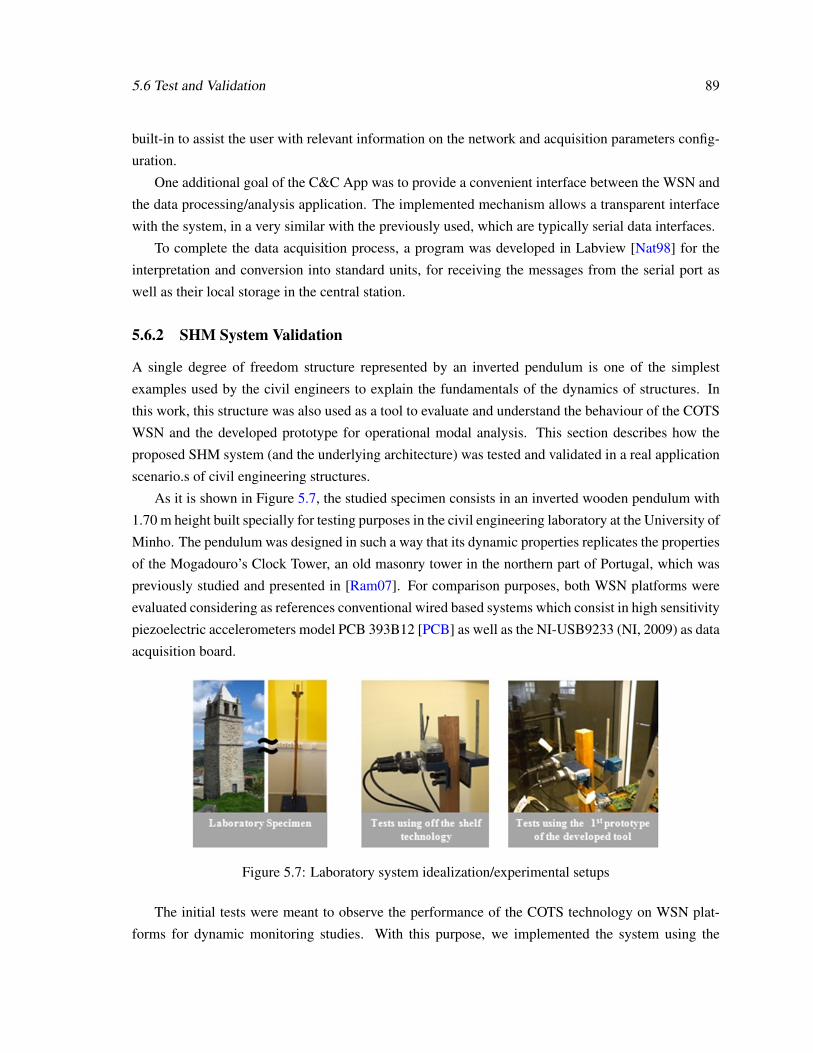
5.6 Test and Validation 89
built-in to assist the user with relevant information on the network and acquisition parameters config-
uration.
One additional goal of the C&C App was to provide a convenient interface between the WSN and
the data processing/analysis application. The implemented mechanism allows a transparent interface
with the system, in a very similar with the previously used, which are typically serial data interfaces.
To complete the data acquisition process, a program was developed in Labview [Nat98] for the
interpretation and conversion into standard units, for receiving the messages from the serial port as
well as their local storage in the central station.
5.6.2 SHM System Validation
A single degree of freedom structure represented by an inverted pendulum is one of the simplest
examples used by the civil engineers to explain the fundamentals of the dynamics of structures. In
this work, this structure was also used as a tool to evaluate and understand the behaviour of the COTS
WSN and the developed prototype for operational modal analysis. This section describes how the
proposed SHM system (and the underlying architecture) was tested and validated in a real application
scenario.s of civil engineering structures.
As it is shown in Figure 5.7, the studied specimen consists in an inverted wooden pendulum with
1.70 m height built specially for testing purposes in the civil engineering laboratory at the University of
Minho. The pendulum was designed in such a way that its dynamic properties replicates the properties
of the Mogadouro’s Clock Tower, an old masonry tower in the northern part of Portugal, which was
previously studied and presented in [Ram07]. For comparison purposes, both WSN platforms were
evaluated considering as references conventional wired based systems which consist in high sensitivity
piezoelectric accelerometers model PCB 393B12 [PCB] as well as the NI-USB9233 (NI, 2009) as data
acquisition board.
Figure 5.7: Laboratory system idealization/experimental setups
The initial tests were meant to observe the performance of the COTS technology on WSN plat-
forms for dynamic monitoring studies. With this purpose, we implemented the system using the

90 Structural Health Monitoring Application Scenario
MICA2 mote platform with a MTS400 board fitted with an accelerometer. The accuracy of the time
series recordings of these platforms was evaluated using only one of the conventional accelerometers
and mote placed at the top of the Pendulum. The results of these tests are presented in Figure 5.8.
The results of the first test indicated the good performance of the commercial WSN platforms for
measuring high amplitude vibrations. As it was expected, for signals with amplitudes below 20 mg,
the WSN platforms recorded only noise (it is even feasible to observe the digitalizing lines) due to
the low resolution of the micro-accelerometers and the ADCs embedded. However, it is important to
state that in SHM studies of civil engineering structures, vibrations with amplitudes below 2 mg are
commonly found. Moderate differences (less than 5%) were found in the frequencies detected with
both systems (wired and COTS WSN) as well as meaningless results for the mode shape detection
task due to the lack of the implementation of synchronization algorithms in the commercial WSN
platforms.
Using the developed prototype of WSN platform, a second round of tests was carried out consid-
ering the same inverted pendulum as case study. The first test was aimed to observe the quality of the
time series recordings of the developed platforms. With this purpose, the effect of an impulse force
was registered using one conventional accelerometer and one new sensing node, both located at the
top of the pendulum. The tests were carried out considering a sampling rate of 100 Hz and sampling
time of 10 s. The results are shown in Figure 5.9.
Figure 5.8: Time domain series recorded using COTS WSN platforms: (a) low amplitude excitationrecordings; and (b) higher amplitude excitation recordings
As it was shown, even for signals with amplitudes below than 0.25 mg, the records from the new
developed WSN platform and the conventional wired based accelerometers presented a remarkable
degree of similarity.
The subsequently stage consisted on the verification of the accuracy of the frequency content of
the acquired signals with the developed WSN platforms. Considering the same pair of sensors located
at the top of the pendulum and 30 s of sampling time, experiments in two excitation scenarios were
carried out: random impacts tests (vibrations with amplitudes below 5 mg) and ambient noise tests

5.6 Test and Validation 91
(vibrations with amplitudes below 1.5 mg). The Welch Spectrum [Wel67] of the time series records
were calculated and are presented in Figure 5.9.
Figure 5.9: Time domain series recorded using the developed prototype of WSN platform: (a) Highamplitude excitation recordings; and (b) lower amplitude excitation recordings
The results evidenced the high accuracy of the resultant frequency domain spectrum calculated
from the records of the new developed system. With this respect, even in the case of ambient noise
tests, outstanding similarities in the content of frequencies were detected.
The last stage of the experimental operational modal analysis process consists on the estimation
of the dynamic properties of the structures by means of their natural frequencies, damping coefficients
and mode shapes. For this purpose, a more refined data processing method was used which consisted
on the evaluation of the time series recordings with 3 conventional and new developed sensors located
at the top of the pendulum using parametric time domain techniques such as the Stochastic Subspace
Identification (SSI) method [VODM91]. Figure 5.10 shows the results of this analysis for the case of
random excited system.
The first two mode shapes of the structure were identified with no uncertainties. However, there
was registered a light difference in the third mode shape which will be further investigated. Table 2
summarizes the results of the experimental modal identification studies performed in the pendulum
using the conventional wired based systems and new WSN platforms.
Table 5.2: Modal identification results
Conv. Systems WSN Prototype ErrorMode f (Hz) ζ (%) f (Hz) ζ (%) ∆ f (%) ∆ζ (%)
1 3.26 2.0 3.34 2.4 2.5 20.02 5.00 2.3 4.94 1.9 1.2 17.43 16.07 1.2 16.03 2.0 0.3 66.7

92 Structural Health Monitoring Application Scenario
Figure 5.10: Frequency domain results – Tests new WSN Platform
5.7 Final Remarks
Accurate synchronization is of crucial importance for these kinds of SHM applications. Synchro-
nization is tightly coupled with timeliness both at software and hardware level, in such a way that to
guaranty tight synchronization we must also take into consideration several aspects such as the task
management strategies of the Operating System, processing time, interference from external sources
and clock drift.
In effect, precise synchronization with a non-real time operating system such as TinyOS can be
hard to achieve, and additional effort was made to ensure that no other tasks would run while process-
ing a beacon frame. In this line, and due to the limited data processing and storage capabilities of the
host WSN platform, the control of the data acquisition had to be transferred to a secondary processing
unit, integrated in the SAB.
This unit runs a real-time firmware supporting all the hardware of the SAB and managing data
processing, synchronization error detection and data storage (up to 32 MB of samples), thus freeing
the TelosB microcontroller from these tasks, in order to become dedicated to communications and
stack management.
Concerning the custom hardware we designed, the Signal Acquisition Board (SAB) gathered sev-
eral different modules: the front-end input from the acceleration sensor, acquisition channel multiplex-

5.7 Final Remarks 93
ing, analogue signal filtering and conditioning, high resolution analogue to digital conversion (ADC),
energy supply/management, data processing/storage, and communication/integration with WSN host
platform. Combining all these building blocks in a single board is a very demanding task in terms of
system dimensioning and design, as characteristics like low-power consumption and energy efficiency,
analogue signals filtering and conditioning, high resolution ADC, low-noise, digital signals and digital
data processing/communication, are typically opposing each other terms of design requirements.
The small-scale prototype was deployed at Mogadouro’s Clock Tower in Bragança, Portugal. We
observed a few connectivity problems with the sensing nodes, although the distance to each other was
not very significant (less than 15 m). In fact the orientation of the TelosB mote had an important
impact in the communication range, and moreover, the walls greatly attenuated the radio signal, thus
limiting the coverage of the deployment. This experience besides validating the small-scale prototype
with positive results, proved that our research work towards a synchronized and scalable SHM system
with routing support was definitely a safe bet in order to enable larger scale and accurate SHM.
The work hereby presented, describes a wireless sensor network (WSN) system for monitoring
physical infrastructures. Building upon the cons of traditional wired-based solutions, several solutions
based on WSNs have been proposed, but there was a lack of ready-to-use and off-the-shelf WSN
technologies able to fulfil some more demanding requirements of these applications (e.g. monitoring
bridges, historical buildings or vehicles structures).
Here, we describe a solution that is mostly based on standard and off-the-shelf technologies,
namely in what concerns hardware platforms, operating system and communication protocol. Only a
minimum set of custom-designed signal acquisition hardware was conceived, in order to serve as an
interface between the accelerometers and the sensing nodes. Our solution is low-cost and guarantees
accurate and time synchronized measurements.
In the long term we aim at deploying a larger and multiple-cluster network in a real scenario. This
however presents a few challenges concerning the network architecture. First, a mechanism must be
devised to support a tight synchronization of the sensing nodes within the different clusters. However,
this is not supported by the legacy IEEE 802.15.4/ZigBee protocols. In this line, a mechanism to
support this is proposed in chapter 8 of this thesis and validated using this SHM application scenario.
Second, increasing the number of clusters might result in an increased and sometimes unbalanced
amount of traffic from the sensing nodes directed at the sink. Thus, the reception of all the sensing data
might take a much bigger amount of time when compared with the star-based single cluster network
hereby proposed.
If in the one hand, a smaller amount of bandwidth allocated to each cluster results in a shorter
beacon period in the network, facilitating the network setup, control and synchronization, on the other
hand, a larger bandwidth allocated to each cluster would decrease the overall transmission time of the
sensing data. This trade-off is addressed with the DCS mechanism proposed in chapter 9 of this thesis
which is also instantiated in this application scenario.

94 Structural Health Monitoring Application Scenario
The design of (distributed) data processing and classification algorithms (for modal analysis and
damage identification) is also envisaged in the future and will also improve our system by reducing
data transmission time. Moreover, it would also further enable the possibility of adding control to the
network to enable systems such as bridge weight-in-motion.

Chapter 6
Datacenter Monitoring ApplicationScenario
6.1 Context and Motivation
This chapter presents another potential application scenario for WSNs which also constitutes an em-
bodiment of the Cyber Physical Systems paradigm. Datacenter Monitoring is increasingly becoming
a hot topic raising energy and security concerns, as the cloud computing phenomena gains momen-
tum. We designed and implemented this application scenario to explore in a hands on perspective, the
most prominent Quality of Service (QoS) challenges such applications could present and to trigger the
design of new mechanisms to solve these. Finally, the objective is to validate and demonstrate in this
scenario the QoS mechanisms proposed in the third part of this dissertation.
Data centers are facilities designed to host large computer systems and have become a crucial
piece in the IT operations of many organizations. A data center can range from a single small room
to several floors or even buildings and consume up to 200 times more electricity than standard office
spaces [WL10]. This large power consumption justifies a special attention to the design of energy
efficient data centers, and there are many approaches to achieve this end. For example, more efficient
server systems, storage devices, network equipment and cooling system can be designed as well as
power or airflow distributions can be improved.
It was commonly understood that electricity consumptions in massive server farms would double
between 2005 and 2010. Instead, most recent reports detail a fully different trend where such number
rose only by 56% worldwide [Koo11] and this slower-than-expected growth stems from a stagnant
economy and the rise of virtualization and cloud-based services. Nevertheless, the average data center
is still largely inefficient. The standard measure of a data center’s efficiency is its Power Usage Effec-
tiveness (PUE), i.e., the ratio between the total energy used to operate a data center and the amount
devoted to actual IT services. The total includes lighting, fans, air conditioners and even electrical
95

96 Datacenter Monitoring Application Scenario
losses in the transfer from the grid to the physical hardware. Ideally, a data center would run at a
PUE of 1.0 and all the electricity would go to computing. However, in the typical data centers this
coefficient is more likely to approach 2.0 [Mon12]. This is because the different elements composing
a datacenter and contributing to the energy efficiency have non-trivial interactions with each other.
Physical parameters, such as power and environmental variables of the data center (e.g., temperature,
humidity, barometric pressure) are often coupled with computations (for example, workload distribu-
tion in the data center). In this sense, we can see the operation of a data center as an instantiation of a
large Cyber-Physical System (CPS).
This chapter reports on the current achievements and ongoing work towards energy-efficient op-
erations and the integrated management of cyber and physical aspects of data centers. The goal is
to develop an integrated system to monitor the power consumption of the servers and their rooms’
environment conditions, with the goal of achieving an overall reduction of the data centers’ energy
consumptions. The proposed architecture is intended to be hierarchical, modular and flexible enough
to achieve a high temporal and spatial resolution of the sensor measurements, with negligible latencies
of sensors’ reports to the data center management control station.
Overall, the advantages of having fine-grained power and environmental measurements in this
application scenario are the following:
(i) Measuring the power consumption at the single server level has enormous benefits for the
business logic of data centers’ owners, since they can offer services and billing to their customers
based on the actual consumption (this project is being carried out in conjunction with a medium/large
service provider in the area (Portugal Telecom), which defined this as an important goal of the system).
(ii) Although there are models in the literature to predict heat-flows used in commercial Computer
Room Air Cooling (CRAC) systems, those models often lack spatial resolution. In this line, the possi-
bility to sense micro-climate conditions, feeding those models with real measurements, will improve
the reliability and accuracy of their forecasts.
Finally, (iii) local actuation, e.g., controlling the power of local in-row CRACs systems or using
directional blades, allows to establish micro-climates and individually act on cooling the most heated
areas, instead of over-cooling the whole datacenter, which leads to energy losses.
Fine-grained measurements also enable to provide different views of the system, each of them
customized to different users. The proposed architecture allows to set the desired resolution of the
readings upon user’s requests, for example to investigate some problems in a specific area (rack, row,
room or floor) of the data center. Every single sensor can be configured by setting user defined alarms
and trigger measurements reports adaptively, by changing or (re-)configuring specific thresholds at
run-time.
Importantly, we propose two approaches for the sensing architecture. The first relies on a cluster-
tree based WSN topology, featuring only wireless sensing devices. The second approach, considers a
mix of wired and wireless devices. Relying solely in wireless devices, although technically possible
6.2 Related Work 97
is still quite costly in large scale deployments, mostly due to the radio transceiver’s cost. Considering
we are aiming at designing a competitive system, also in terms of cost, we had to devise an alternative
architecture to reduce the amount of wireless sensing devices at the expense of reduced flexibility and
ease of installation.
The following sections describe the data collection and distribution system architecture, show-
ing in detail how the environmental and power data will be collected from the data center. Initial
deployment experiments and results are also presented.
Closing this chapter, a set of QoS challenges were identified to further extend the application’s
functionality. These challenges are addressed in Part III of this thesis by proposing a set of QoS mech-
anisms, which are integrated in the design of a crosslayer and online QoS management mechanism,
described in chapter 10 and instantiated in this application scenario.
6.2 Related Work
Thermal management and green data centers have received considerable attention in recent research
literature. Two main approaches can be identified: mechanical design-based and software-based [LKPP10].
The former approaches aim at studying the airflow models, data centers layout and cooling system
design in order to optimize the location of the racks and CRAC units. On the other hand, the latter
approaches focus on minimizing the cooling costs by distributing or migrating jobs among the servers.
The result of this study is the design of thermal-aware scheduling mechanism to distribute the work-
load where the power budget (i.e., the product of power and temperature [HCG+06]) is more favorable.
However, in the current data center thermal management systems, the mechanical and software-based
approaches are usually independent on each other [LKPP10].
Few very recent approaches rely on building software models through a joint coordination of
cooling and load management [PSK08, ZWBM12]. However, the complexity of data center airflow
and heat transfer is compounded by each data center facility having its own unique layout, so achieving
a general model is difficult [RJ07]. In fact, in [PSK08], authors stress that their model has several
parameters that need to be determined for specific applications.
Similar drawbacks affect other models, which formulate an energy minimization problem, subject
to service delay and Quality of Service (QoS) constraints. In this class it is worth to mention dynamic
voltage scaling [BEK+02, HASL07] and on/off power management schemes [XZR+05] – [WCLL10].
Then, acquiring data at a fine enough spatio-temporal resolution to validate models and keep their in-
puts updated at run-time is paramount. Nevertheless, this problem poses new challenges and research
issues concerning the type, number and placement of sensors [RJ07].
Along this line, some recent work [LLL+09, WTS+11] pushed in the direction of deploying wire-
less sensor nodes and monitor the thermal distribution, to figure out how to avoid hot-spots and over-
heating conditions. In [WTS+11], for example, 108 wireless sensor nodes were deployed in a floor

98 Datacenter Monitoring Application Scenario
of the IBM data center in Geneva. We differ from this approach in the sense that we want very fine-
grained (in space and time) gathering of power and environmental parameters and include physical
quantities other than temperature only.
Our approach has similarities to [LKPP10], where authors propose a (proactive) thermal manage-
ment system built upon an air flux mathematical model, which leads to a formulation of a minimization
of cooling energy problem. Moreover, in [VLP11], the same authors developed a joint communication
and coordination scheme that enables self-organization of a network of external heterogeneous sensors
(thermal cameras, scalar temperature and humidity sensors, airflow meters) into a multi-tier sensing
infrastructure capable of real-time data center monitoring. Differently from [LKPP10, VLP11], our
proposed system is based on a hierarchical, modular, flexible and fine-grained sensor network archi-
tecture, where data collected from heterogeneous sensors (including power measurements) and the
analysis of their inter-correlations will enable closer examination and a better understanding of the
flow and temperature dynamics within each data center [SCI05]. To our knowledge, at the time of
this work no previous work enabled correlating power and environment characteristics on a per rack
or per-server granularity.
At the lower tiers, we propose two architectures. One relies on a fully wireless approach, while
the second, similarly to the Microsoft DC Genome project [LA12], uses a network of sensors inter-
connected through a mix of wireless and wired technologies. Contrarily to [LA12], we aim to use
open and Commercial Off The Shelf platforms as much as possible and, to support the wired system
architecture, an industry-based wired bus, such as MODBUS [mod02], instead of USB cables.
Multiple long-wavelength infrared image sensors can be used to capture thermal maps of an en-
vironment [KM05]. While thermal cameras are an interesting approach, we find that they suffer from
several practical issues:
(i) the current cost of thermal cameras is substantial, and, due to field-of-view limitations (data
centers are typically organized in narrow rows), a high number of them should be required to cover a
data center;
(ii) mapping the view of the camera with the infrastructure being monitored is more challenging
than relying on point sensors, and it is especially difficult to manage when changes are made to the
layout of the data center (e.g., addition/removal of servers and racks), and
(iii) by using cameras, the quantitative data analysis would need to be provided by computer
vision, which is feasible, but requires a very specific tuning for each scenario and equipment.
However, as claimed also by authors in [VLP11], our system has provisions to support thermal
image sensors as a smart sensor that can provide temperature field readings with a configurable reso-
lution.
As far as the higher tiers of the system architecture are concerned, the data collection, distribution
and visualization functions need to be carefully addressed. The goal in this case is to provide adminis-
trators and designers with a representation of the actual data center’s conditions in real-time, in order

6.3 Architecture Overview 99
to early identify problems and solutions.
In literature, a number of recent work addresses some of these functionalities. The MQ Teleme-
try Transport (MQTT) [Loc10] is a publish-subscribe messaging protocol, designed for constrained
devices. While it is very lightweight and as been successfully applied in several areas [SCW10] –
[GCNS11], it does not provide any flexible mechanism to define messaging format.
The Global Sensor Networks (GSN) [AHS06] supports the flexible integration and discovery of
sensor networks and sensor data. It is a service-oriented architecture, where sensors can be accessed
using SQL queries and web services. However, GSN is substantially single-application centric and
does not support security features.
The proposed solution builds upon previous work in SensorAndrew [RBR11], which defines an
infrastructure for sensing and actuation, using the XMPP protocol (more details about XMPP will be
given later in Section 6.3.2) at its core. It flexibly provides both point-to-point and publish-subscribe
communication, confidentiality, access control, registration, discovery, event logging and management
of sensor/actuator devices.
6.3 Architecture Overview
The architecture of our system is divided into three main sections: (i) The data-producing entities
such as the sensor networks, which gather environmental data, IT equipment or building equipment,
which gather the data from the environment, and also power consumption data. The data from these
sensor networks is delivered to (ii) a data distribution system that acts as a broker between (iii) the
data consuming entities and the consuming applications (e.g., logger applications, alarm monitor, user
interface applications).
At the core of the architecture depicted in Figure 6.1 there is a data distribution middleware, which
takes care of handling the data coming from different sources such as the environmental and power
sensors and deliver this data to the applications interested in this data. The applications can be a data
logger that gathers historical information, visualization tools, alarms monitors or any other application
that can be developed in the future.
In the following subsections, our proposed system architecture will be described in more detail,
highlighting each component of the data gathering and data distribution system.
6.3.1 Environment and Power Data Collection
The environment and power data collection system aims at supporting a trade-off among (i) fine-
grained sensors’ measurement (spatial) resolution, (ii) system flexibility and modularity, (iii) low-
latency reporting of the measurements, and (iv) low cost. Two different approaches were designed
to support the data collection. The first relies on a cluster-tree based WSN topology, featuring only

100 Datacenter Monitoring Application Scenario
Figure 6.1: Architecture Overview. Several types of devices depicted: Sensor Nodes (SN) with sensorsdirectly attached; Wireless Base Stations (WBSs) that collect data from several Sensor Nodes andGateways (GWs) that collect data from WBSs.
wireless sensing devices. The second approach, consists of a mix of wired and wireless devices.
Importanly, both share the upper system application layers.
The reasoning underlying the second approach mostly concerns cost efficiency. WSN technology,
namely transceivers are still quite expensive, and although it is expected that their cost will be reduced
in the following years, this fact remains an impediment to large scale deployments. Considering the
system was developed with a commercial objective in mind, the system should be competitive in
terms of cost. With this in mind, the number of wireless sensing devices was greatly reduced in the
second approach by using a wired bus to interconnect those nodes, taking advantage of the traditional
organization of a datacenter facility in rows of racks.
Independently of this, both proposals were successfully implemented and deployed in a datacenter
and are presented in detail in this section.
The WSN is a stacked multi-tier architecture, also depicted in Figure 6.1. Each level represents
a network tier with the corresponding devices and communication technology used. The lower level,
level-0 consists of sensor nodes, i.e., small computational units with several physical sensors attached,
which perform sensing tasks and deliver data to the devices at the next level in the hierarchy. At
level-1, Wireless Base Stations (WBSs) are responsible for querying the Sensor Nodes within their

6.3 Architecture Overview 101
respective cluster. A cluster is composed by one WBS and several Sensor Nodes. Then, WBSs are
responsible for data aggregation and sensor fusion. They communicate using IEEE 802.15.4 with
devices at the next level in the hierarchy. At the level-2 of the network hierarchy, (environment)
gateways are present. These devices have the highest computational capabilities among the devices
present in the sensor network field. Gateways provide the data gathered from the sensor network to the
data distribution system in a standard format. Finally, in level-3, the data distribution provides means
to deliver the data gathered from the sensor network to the applications. The data distribution system
supports any number of gateways and applications in a distributed and transparent way.
Sensing Units. They are composed of a platform which carries out the data acquisition of digital
environmental sensors, including humidity, temperature and pressure, as well as power sensors to
monitor the power consumption of each server in the rack. These units are able to interface the sensors
using an I2C bus, enabling to extend their sensing capabilities as needed.
Wireless Base Stations (WBSs). The WBSs receive the input from the Sensing Units and carries
out some data aggregation. A common Gateway is in charge of gathering measurements and sending
them over long-range communication technology (e.g., WiFi, Ethernet). In terms of HW platforms,
the WBS node should consist of the same platform as a generic Sensing Nodes.
Gateways. The system can have one or more Gateways. Gateways maintain representations of
the data flows from the sensor network to the data distribution system. They perform the necessary
adaptation of the data received from the WSN. The gateways can be deployed as one per room serving
all the rows of racks in that room; more gateways can also be deployed to improve radio coverage, for
load balancing or for redundancy.
6.3.1.1 Cluster-based WSN Approach
Figure 6.2 presents the network topology used to support the WSN architecture.
The network is organized in a ZigBee cluster-tree network topology. We assign one cluster of
6 Sensor Nodes (i.e. ZigBee End-Devices) to each datacenter’s rack. Each cluster is controlled by
a Wireless Base Station (i.e. ZigBee Cluster-Head) which forwards data to the Gateway, a role that
can be assigned to any router at the top of the tree. Usually, we do not assign the role of sink to the
ZigBee Coordinator. It is better not to burden this node in terms of processing, considering its vital
importance to the network by maintaining synchronization. Instead, a ZigBee router is usually chosen
as a Sink. Hence, the ZigBee Coordinator’s roles are usually limited to network synchronization and
management.
The WBS, in principle are not used for sensing, although this feature can be easily enabled if
needed. Their only tasks are to manage and synchronize their cluster, to aggregate and to forward data
to the gateway.
Interestingly, the IEEE 802.15.14/ZigBee set of protocols, when configured in this network topol-
ogy, are able to provide the flexibility to support the mixed criticality this application imposes. For

102 Datacenter Monitoring Application Scenario
Figure 6.2: Cluster-based Architecture
instance, a major advantage of this network topology is that we can rely on its natural predictability
to support alarms. In this line, the GTS mechanism of the IEEE 802.15.4 can potentially provide this
feature. This is useful to inform the user of high priority events, that may require immediate attention.
These may consist of severe sensor threshold violations, such as an extreme temperature event, or se-
curity violations, such as a physical unauthorized access to a server, triggered by the opening of a rack
door. To support this feature, the IEEE 802.15.4 GTS mechanism was implemented over TinyOS. The
description of this implementation was presented in this thesis in chapter 4.
On the other hand, less critical data in terms of timeliness can also be supported in parallel by
the network using the CSMA/CA mechanism. Importantly, by using a time-division approach in the
scheduling of the several cluster’s active periods, we are able to mitigate the radio interference this
kind of dense deployments are usually so prone to, improving on the network performance.
Concerning the hardware platforms, all the nodes in this architecture consist of TelosB motes [MEM].
These provide temperature and humidity readings through its embedded sensors, although the sensing
capabilities of the Sensor Nodes can be easily extended, via the I2C bus, by connecting other sensors.
The advantage of relying solely on wireless devices, is that it eases the installation process consider-
ably, as the nodes can be placed anywhere, at any time, in any of the racks. This fact also enables
more possibilities for a reconfiguration of the datacenter’s disposition resulting in an improved power
efficiency.
In addition, this approach can support synchronization of the data acquisition process, which al-
though not an initial requirement of the application, it is expected as a future extension.
Power to the nodes can be provided by either batteries (at each node) or through a USB connection,
which is easily available in each rack, the latter being the preferred method.

6.3 Architecture Overview 103
Figure 6.3: Picture of the network deployment at the datacenter.
Figure 6.3 shows a view of the deployment of the cluster-based approach in a datacenter. The
TelosB nodes in the figure are connected via a USB connection for power. Figure 6.4 shows a snapshot
from the Daintree network sniffer showing the network formation.
Upon connection, the ZigBee Coordinator node starts broadcasting beacons to synchronize the
network. Next, the WBS synchronize and associate to it forming the tree structure. The WBS trigger
the formation of their clusters by sending their own beacons according to a previously setup cluster
schedule. At last, the Sensor Nodes in each cluster synchronize and associate to the corresponding
WBS. The ID of each Sensor Node is hard-coded, although a DIP switch will be used in the future
avoiding re-programming. As soon as all the racks are connected and associated, the gateway is
notified, and the user can trigger the data acquisition process.
Using a cluster scheduling time-division approach [KCAT08] the 8 clusters were scheduled as
depicted in Figure ??. Each cluster’s active portion is composed of a contention access period (CAP),
in which most of the data is transmitted, and a contention-free period (CFP), for real-time traffic
support. The CFP was setup to support one GTS slot per each Sensor Node, with the possibility of
supporting 7 nodes at the most.
We divide the alarms into two groups: (1) Threshold Violation, which are triggered by a hard
variation in the data read by the sensors (e.g. high temperature shifts), and (2) Security Violation,
which groups the alarms concerned with security and physical access to the datacenter (e.g. a rack
door opened). Chapter 10 details the network performance evaluation of this setup and the proposed
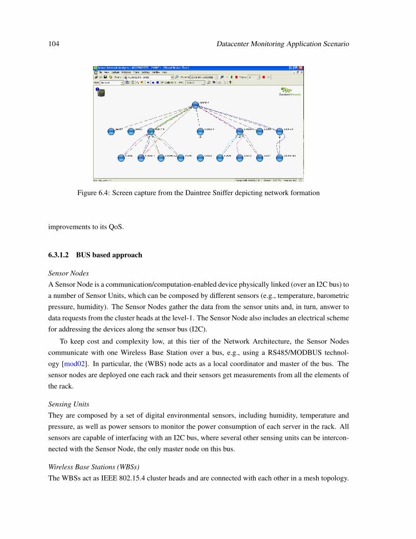
104 Datacenter Monitoring Application Scenario
Figure 6.4: Screen capture from the Daintree Sniffer depicting network formation
improvements to its QoS.
6.3.1.2 BUS based approach
Sensor Nodes
A Sensor Node is a communication/computation-enabled device physically linked (over an I2C bus) to
a number of Sensor Units, which can be composed by different sensors (e.g., temperature, barometric
pressure, humidity). The Sensor Nodes gather the data from the sensor units and, in turn, answer to
data requests from the cluster heads at the level-1. The Sensor Node also includes an electrical scheme
for addressing the devices along the sensor bus (I2C).
To keep cost and complexity low, at this tier of the Network Architecture, the Sensor Nodes
communicate with one Wireless Base Station over a bus, e.g., using a RS485/MODBUS technol-
ogy [mod02]. In particular, the (WBS) node acts as a local coordinator and master of the bus. The
sensor nodes are deployed one each rack and their sensors get measurements from all the elements of
the rack.
Sensing Units
They are composed by a set of digital environmental sensors, including humidity, temperature and
pressure, as well as power sensors to monitor the power consumption of each server in the rack. All
sensors are capable of interfacing with an I2C bus, where several other sensing units can be intercon-
nected with the Sensor Node, the only master node on this bus.
Wireless Base Stations (WBSs)
The WBSs act as IEEE 802.15.4 cluster heads and are connected with each other in a mesh topology.

6.3 Architecture Overview 105
RS485
C
CBUFFER
I2C SWITCH
BUFFER I2C SWITCH
µC
TP
BUFFER BUFFER
µC
Power Meter
Sensor Node
H
Sensing Unit(Environment)
Sensing Unit (Power)
802.15.4
µC
RS485
WBS
Figure 6.6: Hardware Platform Architecture
A common Gateway is in charge of gathering measurements and sending them over long-range com-
munication technology (e.g., WiFi, Ethernet). In terms of HW platforms, the WBS node will be the
same platform as a generic Sensor Node, with an on-board ZigBee radio. Thus, each Sensor Node can
become a WBS with minimal modifications, i.e., just by plugging the wireless module and uploading
a different firmware.
Gateways
The sensor network can have one or more Gateways. Gateways maintain representations of the data
flows from the sensor network to the data distribution system. They perform the necessary adaptation
of the data received from the WSN. The gateways can be deployed as one per room serving all the
rows of racks in that room; more gateways can also be deployed to improve radio coverage, for load
balancing or for redundancy.
Figure 6.6 puts forward some additional details about the low level sensing devices. The WBS is
directly connected to a power source and supplies power through a twisted pair cable to all the Sensor
Nodes in that bus. In all the nodes on this bus, the voltage is locally converted to lower values by a
step-down switched power supply for higher system efficiency. Wires running in the same cable form
a serial data bus (MODBUS over a RS485 connection) that connects the Sensor Nodes.
The Sensor Node is composed by (i) an RS485 interface for the MODBUS, (ii) 6 on-board current
sensors (denoted as C in Figure 6.6), (iii) one I2C switch, responsible for duplicating the bus capacity
in terms of addressable devices, and (iv) the buffers on its output, which increase the electrical robust-
ness of the I2C bus over longer distances. Power is also present in the cable which carries the I2C
bus, again locally regulated in every Sensing Unit for a higher quality voltage supply for the sensor
devices.
The environmental Sensing Units are composed by digital sensors of humidity, pressure and tem-
perature, with configurable resolution for trading between higher resolutions and lower conversion
times. The Sensing Units may have different sensor arrangements (for example, only a temperature
sensor, or only a pressure sensor), such that they are more customizable to the actual sensing needs.
The Sensor Units form a network over the I2C bus. Each Sensor Node can be connected on the

106 Datacenter Monitoring Application Scenario
I2C bus with up to 52 temperature sensors, 54 power meters, 14 pressure sensors and 14 humidity
sensors. Moreover, Figure 6.6 shows that the Sensor Units also have an I2C switch, needed to address
sensors that have a fixed address, and cannot be in the main bus.
For the design of the I2C network, some basic requirements have been considered:
(i) the sensors should be grouped and sampled according to the physical quantity observed, for a
lower latency between measurements of a given cycle, and a better temporal granularity;
(ii) this Sensor Units network has to be modular, where Sensor Units can be added or removed at
run-time without interrupting the sampling service;
(iii) the maximum cycle time for sampling all the sensors should be the minimum conversion time
required for each sensor, depending on its operating precision. This defines the sampling time required
for reading all the sensors and also the maximum number of Sensor Units allowed on the bus;
(iv) when queried, guarantees must be given for the maximum response time of the Sensor Node,
to the level-1 network. This is important to ensure bounds on communication between the Sensor
Nodes and the WBS.
The I2C bus can also include Power Meter Units, which are buffered and driven by a microcon-
troller, responsible for reading the power consumption information from a dedicated microchip. This
microchip interfaces with the power line and provides detailed information about the power consump-
tion. These power meters can provide true power readings and complement the current sensors on the
Sensor Node board.
Task 1
Task 2
Task 3
Task n
Listening
treqtreqi tidle tread treq
treply
s
Figure 6.7: Task Scheduling at the Sensor Node
To ensure latency bounds on the queries of the Sensor Nodes by the WBS, an appropriate schedul-
ing of all the activities in the Sensor Node, such that a large number of sensors could be acquired
within a short amount of time, is paramount. The task scheduling scheme of a Sensor Node is il-
lustrated in Figure 6.7. Every line represents a task, where the numbered lines represent the tasks
responsible of sampling the sensors individually, up to ns sensors in the bus. The time interval treq
represents the sum of the time needed to request every sensor for a conversion. The time interval tidle

6.3 Architecture Overview 107
DataCentre(
Room(1( Room(2(
Row(1( Row(2( Row(3( Row(…(
Rack(1( Rack(2( Rack(3( Rack(…(
DataCentre(Master(Node(
Room(Master(Nodes(
Row(Master(Nodes(
Aggrega9on(of((sensor(nodes(
(a) Hierarchy of the XMPP Event Nodes.
XMPP$$Server$ Virtual$
Physical$Virtual$Logical$
Aggregator$
Virtual$Physical$
Virtual$Logical$
Desktop$ Laptop$ Mobile$
Real$Node$
Real$Node$
Real$Node$
Real$Node$
Real$Node$
(b) XMPP Event Node Data Aggregation
Figure 6.8: XMPP Event Nodes Hierarchy and Data Aggregation
depends on the sensor conversion time and the time required to query all the sensors (treq) in the bus.
During tidle the Sensor Node is idle, but listening to the MODBUS and ready to receive any query
from the WBS.
The time interval tread represents the time required to read the converted values at the sensors. At
the end of tread , the cycle restarts. The worst-case response time of every Sensor Node is given by:
treq + tread + treply, where treply is the time to reply to a query from the WBS (on the RS485/MODBUS
bus). We can see the reasoning for this by observing that, if a query arrives at a point where treply would
overlap tread , the data collection from the sensors will be postponed until the next cycle. There is a
tradeoff between the maximum number of Sensor Units per Sensor Node and the maximum number of
Sensor Nodes per WBS. In our choices, the latter value is defined as 20, as most rows in the datacenter
are generally smaller, and assuming to install a WBS per row.
In the worst case, the WBS node would need nsn× (treq + tread + treply) to query all the Sensor
Nodes on the RS485/MODBUS network, where nsn is the number of Sensor Nodes on the bus.
The design choices for this tier of the network architecture allow for the prediction of the worst
case response time on the first two levels, which enables to better define how real-time requirements
are met. Each sample of data is time stamped at the WBS, then forwarded through the IEEE 802.15.4
interface. The clock synchronization is done periodically, through the broadcast of a special data
packet, coming from the Gateway, responsible to set the clock of every WBS. WBSs are also in charge
of performing local computations on the collected measurements, in order to early estimate a few
metrics about the local-climate, airflows due to pressure gradients, or abnormal power consumption.
This is with respect to the design principle of distributing the intelligence in the system at the lowest
tier as possible: by this, a WBS can raise alerts or detect unwanted conditions, instead of merely
monitoring and reporting data from each individual sensor.

108 Datacenter Monitoring Application Scenario
6.3.2 Data Distribution
The data distribution middleware is a central part of the proposed architecture. This system is in
charge of distributing the data from the source to the interested applications. We leverage on the
previous experience of SensorAndrew [RBR11] and employ the eXtensible Messaging and Presence
Protocol (XMPP) [XMP] as the core protocol for managing sensor data collection and distribution. In
this architecture, sensors (and actuators) are modeled as XMPP event nodes in a push-based publish-
subscribe architecture. The loose coupling between publisher and subscribers allows higher scalability
and more dynamism in the network topology. Moreover, this architecture supports the following
features [RBR11, XMP]: (i) standard messaging protocol; (ii) extensible message types; (iii) point-
to-point and multicast messaging; (iv) data tracking and/or event logging; (v) security, privacy and
access control; (vi) registration and discovery services and (vii) redundancy and Internet-scale.
The XMPP [XMP] is the basis for the messaging of our system. XMPP is an open-standard
communications protocol for message-oriented middleware based on Extensible Markup Language
(XML). Unlike most instant messaging protocols, XMPP uses an open systems approach of develop-
ment and application. That is, anyone may implement an XMPP service and interoperate with other
organizations’ implementations. The architecture of an XMPP network runs in a fully distributed
fashion. XMPP has extensions for several models, including one-to-one communication and publish-
subscribe model, and can be location-aware. It has built-in authentication with support for secure
channels (SSL and TLS) and supports storage of messages for later delivery. XMPP applications in-
clude network management, content syndication, collaboration tools, file sharing, gaming, and remote
systems monitoring. Finally, XMPP is implemented by a large number of clients, servers, and code
libraries, and most of this software is distributed as free and open source.
One of the keys that drove our design choices was to note that this architecture supports several
clients. For example, we can simultaneously have: (i) a logger application that subscribes to all nodes
and simply logs all the data; (ii) an application that subscribes to specific events nodes that deliver
alarm notifications; (iii) an application that is only interested in the data for a particular row of the
data center; (iv) an application that, for management and configuration purposes, only needs to know
when a new device is added to the system; (v) an application that is only interested in power readings.
More details on the organization of the messaging system will be given in the following section.
6.4 Mapping The World
The messaging system was defined to relate to the data center perspective and was structured in a
hierarchical fashion. As we will describe next, this hierarchy reduces the number of data items (event
nodes) that a user application needs to subscribe to and also allows for the user applications to zoom-in
the data center in a flexible manner.

6.4 Mapping The World 109
(a) Datacenter Rack View (b) Rack List View
(c) Historical Data Graph View
Figure 6.9: GUI Views
The hierarchy is defined by an XML schema that includes 3D geographical and logical information
of all elements, including sensors, servers, racks, rooms and even buildings or cities. The model
includes hierarchical links: servers can be placed logically inside a rack, racks can be placed inside a
room, and a room can be connected to a building and so on. The logical organization makes it simpler
to organize the hierarchy without depending on the geographical / 3D information of the model. These
levels in a data center context are shown in Figure 6.8(a). This is a logical hierarchy reflected on the
XMPP event nodes, which lives in the XMPP servers. In this way, this hierarchy can be replicated and
load-balanced by using the common mechanisms implemented by the XMPP server.
Using this structure, if an administrator wants to receive data from a given room, the application
only needs to subscribe to that room and automatically he will be subscribing to all the sensors in the
room. The drawback is that this could result in a single client subscribing to a large number of event
nodes, which can be a problem for clients with limited processing, memory and battery life capacities,
such as, e.g., mobile phones.
To address this issue, we extended the regular XMPP event node concept, which is a direct repre-
sentation of physical nodes (e.g., a real sensor node on a rack) to encompass XMPP event nodes which

110 Datacenter Monitoring Application Scenario
can represent a category or a set of nodes with some common logical characteristics (e.g., belonging
to a given room). In this way, a room might have a representation in the messaging system as a virtual
logical XMPP node, and, for example, the temperature values of a room will be published as a trace
over time of the aggregated (e.g., average, minimum or maximum) values of all the measurements
from the sensor nodes belonging to that room, while all those readings will be published on virtual
physical XMPP nodes to be available later for different views. Figure 6.8(b) represents a possible con-
figuration of this mechanism. An aggregator is a piece of software that resides on the XMPP server
or gateways, which is responsible for gathering data from several real sensor nodes by subscribing to
them and producing a stream of aggregated values according to the hierarchy defined.
For providing the user with an overview of the data center conditions, we also built a web-based
graphical user interface (GUI) application that can run in both desktop and mobile devices. Example
views of the application are shown in Figure 6.9. Figure 6.9(a) shows the view after the user zooms
in into a single rack. Here, a representation of the rack is presented, and the user can interact with it;
Figure 6.9(b) shows that it is also possible to navigate through the datacenter using a text-only interface
(in this case, the list of racks in a particular row is shown) and, finally, Figure 6.9(c) exemplifies how
historical data about physical parameters is shown. In this view (historical data), the user may perform
queries about the different types if sensor data collected, using different
Our web application uses a JavaScript library to bridge this module to the sensor network. The
application takes advantage of the technology employed on the sensor network, XMPP, and makes use
of server push notifications. It is a simple and clean interface that gathers all relevant data, allowing
the user to navigate trough a representation of the data center and observe the data collected.
The different views and components are only created with JavaScript upon user’s request. This
contributes to keep the application lightweight and dynamic. For floor plans, maps and graphics the
same approach is being used. The configuration files are interpreted by the server that creates the
images and then sends the already drawn map to the client (user interface). Using this method, any
environment change can be added to the system without affecting the user’s device.
6.5 The Data Center Radio Environment
It is often assumed that the presence of metallic surfaces (such as racks) and power cables suspended
on the ceiling, makes a data center room a harsh environment in terms of radio signal propagation.
Therefore, we conducted an analysis of the radio conditions of a typical data center, to assess the va-
lidity of that assumption and evaluate its impact. The measurements were performed in a data center
(located in Lisbon, Portugal) owned by the largest Portuguese telecommunications operator, Portugal
Telecom (PT), which also provides hosting and cloud-based services. The objective of such measure-
ment campaign was twofold: (i) evaluate the available IEEE 802.15.4 channels for the monitoring

6.5 The Data Center Radio Environment 111
Figure 6.10: Background noise: experimental measurements with a spectrum analyzer [WiS]. Figurereports average, min and max noise levels on the 2.4 GHz ISM band in a real data center environment.
network to be deployed in the data center, and (ii) test the connectivity among IEEE 802.15.4 radios
in the field, in order to identify the requirements for the density of WBSs.
Background Noise
We first acquired the background noise level to evaluate the possible interference on the monitor-
ing network due to external IEEE 802.11/WLANs. To do this, we used a frequency spectrum ana-
lyzer [WiS].
As expected, Figure 6.10 confirms that there are only few IEEE 802.15.4 channels in the 2.4 GHz
band available. In particular, it is clear that two commonly used IEEE 802.11/WLAN channels (ch6
and ch11) constituted a background noise for our intended network.
Then, thanks to its reduced level of interference, channel 26 was the preferred channel for our
measurements. In general, these background noise measurements show that the number of available
channels in a typical data center might be low.
WSN Connectivity
For the connectivity measurements, we used 9 TelosB nodes (a GW and 8 routers) running on batteries
and 3 TelosB acting as sniffers and attached to the USB ports of a notebook for power and data logging.
The routers were placed at the top of the center rack of 9 rows on a data center.
First, we checked the connectivity between routers. For this, we placed the GW on a corner of
the data center and the routers (R1-R8) were placed on the center of the rows. This experiment tested
that the chain among the GW and all the routers was working, i.e., the GW started emitting beacons,
R1 gets these beacons, associates to the GW and start emitting its own beacons. Then R2 gets R1’s
beacons, associates with R1 and starts emitting its own beacons, and so on until R8. At run time, all

112 Datacenter Monitoring Application Scenario
(a) Packet loss ratio as a function of the distance.
(b) RSS as a function of the distance.
Figure 6.11: Data Center Room Radio Measurements - Overall
routers were able to emit non-interfering beacons, on a time-division fashion.
Then, we started taking measurements with the 3 sniffer nodes as follows. First, we placed the 3
nodes on one half of the row and then on the other half of the row (the 3 nodes were spaced about
1.5 meters from each other, where the one farthest from the middle was 5 meters from the center),
then we collected packets for 5 minutes in each half section of the row and repeated this procedure
for 9 rows. A counter in the beacon payload was set to be incremented at each transmission and
transmission power was set to the maximum. By extracting the source address and the counter in
the beacons from the sniffers’ logs we measured the packet loss probability on each measurement
point and with respect to each router, as well as information about the Received Signal Strength (RSS)
of each received packet. By combining these data, it was possible to build maps of the coverage
for each beacon emitter. Figure 6.11(a) shows the packet loss ratio as a function of the distance
between any transmitter and receiver pair. Similarly, Figure 6.11(b) represents the behavior of the
RSS measurements. Looking at these results, it is evident how the packet loss grows when the distance
between transmitter and receiver increases, i.e., when the received signal power decreases. However,

6.5 The Data Center Radio Environment 113
the packet loss is better than what one could have expected: in general the majority of the routers
was able to cover half of the room with negligible losses (i.e., the average packet loss ratio is always
below 5%). The worst coverage, i.e., the greater values of packet loss, are well localized and due to
some specific conditions. This is better evidenced in Figure 6.12, where the coverage performance for
two nodes, e.g., the GW and the cluster head R1, is shown. Clearly, only spots of connectivity loss
areas were evidenced in proximity of the pillars in the room: these conditions can be easily solved by
accurately planning the position of the routers (cluster heads).
(a) Coverage of GW (R0). Left: packet loss ratio. Right: RSS.
(b) Coverage of R1. Left: packet loss ratio. Right: RSS.
Figure 6.12: Data Center Room Radio Measurements - Details

114 Datacenter Monitoring Application Scenario
6.6 Final Remarks
Instrumenting data centers with very fine spatial and temporal granularity presents a twofold advan-
tage. First, by improving energy efficiency, by having a better control of the micro-climate conditions
in the rooms. Second, in a business case, for data centers’ owners, by providing the possibility of
billing the consumed energy to their clients.
This chapter presents an efficient, hierarchical and modular system architecture, with two ap-
proaches to carry out the data acquisition. The first relies on a cluster-tree based WSN topology,
featuring only wireless sensing devices. The second approach, consist in a mix between wired and
wireless devices. The latter is mostly motivated by the need to reduce the overall system cost, which is
accomplished by reducing the number of wireless devices, by mixing a wired infrastructure. Still, this
architecture is built as modular as possible and can enable an interesting trade-off between fine-grained
monitoring and low-latency.
Nevertheless, despite the cost of the transceivers, which is expected to decrease in the follow-
ing years, the cluster-tree based architecture offers much more interesting features. Among these, it
can support higher flexibility by instrumenting each rack independently without the need for a wired
infrastructure. This enables more possibilities for a reconfiguration of the datacenter’s disposition
resulting in an improved power efficiency. The wireless approach is also being designed to support
a mixed criticality in terms of communications, consisting in a far more complete but also complex
approach regarding the network architecture.
For instance, there are specific alarms which are expected to be triggered and forwarded to the user
within tight deadlines, to guarantee an immediate response to the detected problem (e.g. detection of
a non-authorized physical access to a rack). In this line the legacy IEEE 802.15.4 protocol can provide
a good amount of predictability to these alarms through its GTS mechanism. However, the GTS
mechanism is usually absent from most implementations of the protocol stack such as in the case of
the official TinyOS IEEE 802.15.4 implementation [Tina]. In order to support this mechanism in this
application, we implemented the GTS mechanism (refer to chapter 4) and it is now available to the
community within the official TinyOS release.
There is also less critical data, which constitutes the largest amount of the sensed data (tempera-
ture, humidity and pressure). Nevertheless, although this data can be delivered within a more relaxed
deadline, there are still constraints.
Although, a priori temperature or humidity data monitoring do not seem too challenging in terms
of timeliness, this scenario does not constitute a typical environmental monitoring case. First, it is
expected that the datacenter’s environment data can be used to accurately model the room’s environ-
ment dynamics so that the users can understand with a good granularity the impact of the cooling
equipment, minimizing energy consumption by cooling only where and when needed. This demands
for a scalable and global synchronization of the samples on demand. However, this is not supported

6.6 Final Remarks 115
by the legacy IEEE 802.15.4/ZigBee protocols. In this line, a mechanism to support this is proposed
in chapter 8 of this thesis.
In addition, it is intended that the user have the possibility to zoom in specific zones of the datacen-
ter by increasing the data sampling rate of specific racks, and without loosing the remaining data. This
raises two kinds of concerns: (1) the network must cope with an unbalanced and increasing amount
of traffic, which demands for an efficient management of the available bandwidth, and if possible, a
dynamic allocation of it; and (2) there must be mechanisms in place to support different traffic classes
within the network, so that particular racks (i.e. nodes or clusters of nodes using a networking spe-
cific terminology) can be differentiated from the remaining data, having an increased probability of
successfully accessing the communication channel, considering CSMA/CA is used. This should be
supported on demand.
The first concern is tackled by the proposal of DCS in chapter 9, in which a way to dynamically
adapt the bandwidth given to each cluster is presented. The second issue is addressed by the TRADIF
mechanism, which has been already proposed in the past and we evaluate experimentally in this thesis
in chapter 7. This mechanism initially proposed for a star-based network, is also extended to a mul-
tiple cluster topology in chapter 9. In the latter, a several mechanisms (SSYNC, DCS and TRADIF)
are joined into a cross-layer and online QoS management proposal which is instantiated into this dat-
acenter monitoring application scenario, supporting the aimed on-demand application mode changes.
We have also made a study on the radio performance in a real data center. This study enabled us
to better understand the radio conditions in these kinds of environments. Our findings confirm reports
by previous work [LLL+09, WTS+11, LA12]: even in a data center room of reasonable dimensions,
each wireless node can interfere with up to 65% of the nodes. Then, having too many nodes interfering
with each other is an obstacle towards gathering sensor readings with high temporal resolution. This
fact constitutes another reason to rely on time division strategies to support the network scalability, by
relying on hierarchical cluster-based approaches instead of the traditional mesh-based approaches.
It is expected that the proposed network architecture, fitted with the mentioned QoS add-ons, will
serve as a model for future deployments in similar application scenarios.

116 Datacenter Monitoring Application Scenario

Part III
QoS Improvement Mechanisms
117


Chapter 7
Peformance Evaluation of a TrafficDifferentiation Mechanism
7.1 Introduction
Although some WSN applications like environmental monitoring or precision agriculture, do not im-
pose stringent timing requirements on data delivery, there are a number of other applications in which
timeliness is of great importance. It is the case of most industrial automation and process control ap-
plications, in which computations and communications must not only be logically correct but also be
produced on time. This is also the case of a typical Datacenter Monitoring application scenario such
as the one described in chapter 6 of this thesis.
In that particular scenario, for instance, we can find a mixed criticality in terms of communica-
tions. On the one hand, there are specific alarms which are expected to be triggered and forwarded
to the user within tight deadlines, to guarantee an immediate response to the detected problem (e.g.
detection of a non-authorized physical access to a rack). On the other hand, there is less critical data,
which constitutes the largest amount of the sensed data (temperature, humidity and atmospheric pres-
sure). Nevertheless, although this data can be delivered within a more relaxed deadline, there are still
constraints.
Although, a priori, temperature or humidity data monitoring do not seem too challenging in terms
of timeliness, this scenario does not constitute a typical environmental monitoring case.
Among the requirements, the user should have the possibility to zoom in specific zones of the
datacenter by increasing the data sampling rate of specific racks, and without loosing the remaining
data. This raises two kinds of concerns: (1) the network must cope with an unbalanced and increas-
ing amount of traffic; and (2) there must be mechanisms in place to support different traffic classes
within the network, so that those particular racks (i.e. nodes or clusters of nodes using a networking
119

120 Peformance Evaluation of a Traffic Differentiation Mechanism
specific terminology) can be differentiated from the remaining data with an increased probability of
successfully accessing the shared communication channel.
To enable such systems, the standardization efforts of the IEEE Task Group 15.4 have contributed
with the definition of the IEEE 802.15.4 protocol for Low-Rate, Low-Power Wireless Personal Area
Networks (WPANs). In beacon-enabled mode, this standard provides two mechanisms (check Sec-
tion 2.2.2 of this thesis): (1) slotted CSMA/CA as a Medium Access Protocol in the Contention
Access Period (CAP) and (2) Guaranteed Time Slots (GTS) in the Contention Free Period. The GTS
mechanism enables a deterministic access to the medium but it has some limitations.
The first limitation concerns the restriction on the distribution and amount of traffic that can avail
this service. In a superframe, a maximum of seven GTS slots can be allocated, implying that in each
cluster (PAN) a maximum of seven nodes can have guaranteed slots in any superframe. The remaining
nodes may only transmit in the CAP, without any QoS support.
Second, GTS can only provide guaranteed services in bursts, limiting any node to the length of
the slot allocated to it. This does not provide an optimum solution if the messages requiring QoS
support are evenly distributed over time. Third, even in applications where the limited number of GTS
slots can be considered sufficient, the allocation must be preceded by an allocation request message
transmitted in the CAP, and since collisions may occur, the request may fail, delaying its service.
The same problem applies to other protocol command units. Therefore, network management (e.g.
GTS allocation requests, alarms, network management commands, association commands), are more
critical than regular data frames. Failing to cope with this may result in unfairness and degradation
of the network performance, particularly for high traffic loads. In this line, these critical messages,
require that QoS support be extended to the CAP.
Moreover, the GTS mechanism may also face coexistence problems since other wireless networks
operating in the same frequency range (Bluetooth or IEEE 802.11) are completely unaware of the time
slot allocations made at the IEEE 802.15.4 superframe. This turns the GTS approach worthless in the
presence of collisions. Therefore, while GTS is considered a good solution for the QoS requirement of
the low-rate WPAN applications (for which IEEE 802.15.4 was originally designed), the requirements
of dense sensor networks (especially at high and distributed loads) demand a more flexible mechanism.
The work described in this chapter builds upon a previously proposed [KANS06] set of mecha-
nisms to provide QoS to the CAP (demonstrated through simulation), and describes its implementa-
tion and experimental validation. We show that these mechanisms can easily provide increased QoS
to higher priority messages, requiring only minor add-ons and ensuring backward compatibility with
the IEEE 802.15.4 standard protocol.
The integration of these mechanisms in IEEE 802.15.4 is relevant for leverage its use in time-
sensitive WSN applications.

7.2 Related Work 121
7.2 Related Work
The improvement of the IEEE 802.15.4 Slotted CSMA/CA MAC mechanisms to achieve reduced
(soft) delay guarantees and better reliability of time-critical events on Wireless Sensor Networks has
drawn a few research works. In [HLhAC05], the authors modified the slotted CSMA/CA algorithm
to enable fast delivery of high priority frames in emergency situations, using a priority toning strat-
egy. Nodes that have high priority frames to be transmitted must send a tone signal just before the
beacon transmission. If the tone signal is detected by the PAN Coordinator, an emergency notifica-
tion is conveyed in the beacon frame, which alerts other nodes with no urgent messages to defer their
transmissions by some amount of time, in order to privilege high priority frame transmissions at the
beginning of the contention access period. In [KC06], the authors extend the previous schemes by
allowing high priority frames to perform only one Clear Channel Assessment (CCA) operation in-
stead of two, using a frame tailoring strategy, which aims to avoid collisions between data frames and
acknowledgment frames when only one CCA is performed. This approach of CCA reduction requires
Frame Tailoring, i.e. adjusting data packet length in such a way that one CCA becomes sufficient to
detect any acknowledgement frame transmission. While this method reduces the CCA overhead by
half, problem of backward incompatibility remains.
PECAP [JLKK07] presented yet another solution based on a toning signal. Here, the main idea
was to use the inactive portion of the superframe to carry out the transmission of high priority packets.
The beginning of this portion is signaled by a jamming signal at the end of the CAP. This approach
does not tolerate the use of the CFP for transmitting guaranteed traffic. Although these solutions seem
to improve the responsiveness of high priority frames in IEEE 802.15.4 slotted CSMA/CA, they re-
quire a non-negligible change to the IEEE 802.15.4 MAC protocol, thus turning them non-compatible
with the standard. The toning mechanism imposes some changes to the hardware (using a tone sig-
nal transmitter) and also to the protocol itself, due to the frame tailoring strategy. This represents a
major drawback for these proposals since they contradict the ongoing 15.4 working groups standard-
izations efforts. Other approaches that do not present such an inconvenient have been proposed in the
meanwhile to support service differentiation. These are usually similar to the strategy implemented in
[IEE05].
The IEEE 802.11e specified a Hybrid Coordination Function (HCF) by defining variable parame-
ters such as Arbitrary Interframe Space (AIFS), CWmin and CWmax. This amendment was approved
and incorporated in IEEE 802.11-2007 [IEE07] specification.
Recent research works in IEEE 802.15.4 have presented priority-based service differentiation
models similar to HCF, by tuning of some of the MAC parameters as the Backoff Exponent (BE)
and Contention Window size. In what follows, we enumerate some of those proposals that are focused
on the slotted CSMA/CA. So far, most of the work concerning traffic differentiation either relies on
Markov Chain models or on simulation work. In fact, to our best knowledge, besides our work, there

122 Peformance Evaluation of a Traffic Differentiation Mechanism
is only one proposal that presents an experimental validation in a real WSN platform [KWHK08].
Concerning analytical and simulation work, [KKY+07] presented a Markov chain model and
analysed the impact of changing the backoff and contention window concerning delay and through-
put. More recently in [NKDM09] the authors modeled a differentiation scheme based in two priority
classes. The differentiation was achieved by changing the CWinit value between one and two. Al-
though results were interesting, changing the contention window to one may cause collisions with
ACK frames.
This strategy of tuning a set of MAC parameters to improve the performance of a traffic category
has been used by other recent works. In [BSR09] the authors introduced a backoff paramenter change
to improve the responsiveness of a network control system. The authors used Matlab/Simulink to
simulate the control system and evaluate its response. In DBP [SMM+09] the authors introduced a
(m,k)-firm deadline task model to assign priorities to messages. The Backoff parameters were changed
according to the proximity to lose m deadlines within a window of k service requests, and implemented
the model in MICAz platforms. However, no thorough evaluation of the effects of the parameter
change was carry out in any of these studies. ANGEL [KWHK08], presents, the only implementation
and performance evaluation in a WSN platform (Tmote Sky) of a traffic differentiation mechanism, so
far. Their approach is based on a multi-queue service implemented in a layer above the IEEE 802.15.4
MAC sub-layer. Traffic differentiation is achieved by tuning some MAC parameters.
However, in their work, the effect of each parameter was not studied separately, and the per-
formance evaluation was only focused on changing the macMinBE and macMaxBE parameters, al-
though it was stated that it was possible to change others. Moreover, the implementation was evaluated
over TinyOS [Tin15] which we find unreliable when facing large amounts of traffic due to its lack of
preemption and its FIFO-based task management aproach, making it difficult to precisely identify
the impact of the parameter variations at heavier traffic loads, as described in [CSP+08]. Also, in
[KWHK08], if a lower priority message is already being transmitted by the slotted CSMA-CA algo-
rithm and a higher priority message arrives at the higher priority queue, the transmission is aborted
so that the higher priority message can be transmitted. This preemptive approach may lead to the
starvation of lower priority traffic under certain conditions.
In the remaining of this chapter, we describe a thorough experimental validation of a set of traffic
differentiation mechanisms, previously presented in [KANS06] which are completely backward com-
patible with the standard protocol. This work proposed two mechanisms to achieve traffic differentia-
tion in IEEE 802.15.4 beacon-enabled networks: (1) a single FIFO queue supporting different traffic
priorities by tuning the macMinBE, aMaxBE and CWinit MAC parameter, and (2) a multi-queue
strategy in which different parameter values were assigned to the different queues. Its improvement
was verified by simulation with the OPNET [OPN15] Open-ZB IEEE 802.15.4/ZigBee simulation
model [JK07]. Now we implemented it over a real-time operating system. Moreover, we would like
to assess if such a simple approach is sufficient to satisfy the requirements of time-critical messages

7.3 Traffic Differentiation Strategy 123
and can provide interesting results with current WSN technology.
7.3 Traffic Differentiation Strategy
As shown in [KANS06], the behavior of slotted CSMA/CA is mostly affected by four initialization
parameters, which are: (1) the minimum backoff exponent (macMinBE), (2) the maximum backoff
exponent (aMaxBE), (3) the initial value of the CW (CWinit) and (4) the maximum number of
backoffs (macMaxCSMABackoffs).
Changing the value of any of these parameters will have an impact on the performance. For
instance, a performance valuation study in [KAT06] has shown that the average delay of broad-
cast frames increases with macMinBE, whereas the probability of success remains independent of
macMinBE in large-scale WSNs. However, the probability of success increases for high macMinBE
values, in small-scale WSNs. Based on those observations, we propose to offer differentiated services
for time-critical messages. In this work, our service differentiation mechanisms are particularly based
on the macMinBE, aMaxBE and CWinit parameters. Note that IEEE 802.15.4 defines two frame
types: (1) data traffic, which typically represents sensory data broadcasted to the network (without
using acknowledgments), (2) and command traffic, which comprises critical messages (such as alarm
reports, PAN management messages and GTS allocation requests) sent by sensor nodes to the PAN
Coordinator. Due to their importance, command frames are sent using acknowledged transmissions
and require a particular QoS support to be delivered to their destination in a bounded time interval. In
this work, we consider command frames as the high priority service class and data frames as the low
priority service class.
The differentiated service strategies are presented in Figure 7.1. The idea is simple. Instead of
having the same CSMA/CA parameters for both traffic types, we assign each class its own attributes.
We denote [macMinBEHP, aMaxBEHP] and CWHP the backoff interval and the contention window
initial values for high priority traffic related to command frames, and [macMinBELP, aMaxBELP] and
CWLP the initial values for low priority traffic related to data frames. While, the slotted CSMA/CA
described in Section 2 remain unchanged, the adequate initial parameters that correspond to each
service class must be applied. In addition to the specification of different CSMA/CA parameters,
Priority Queuing can be applied to reduce queuing delays of high priority traffic (Figure 7.1). In this
case, slotted CSMA/CA uses priority scheduling to select frames from queues, and then applies the
adequate parameters corresponding to each service class. Note that if a low priority frame is selected,
i.e. the high priority queue is empty, then the backoff process corresponding to this frame will not
be preempted by a high priority frame arriving during that service time. It will have to wait until the
low priority frame is sent, or rejected if the maximum number of backoff is reached. The heuristics
for adequately setting the CSMA/CA parameters are the following. Intuitively, a first differentiation
consists in setting CWHP lower than CWLP. It results that low priority traffic has to assess the channel

124 Peformance Evaluation of a Traffic Differentiation Mechanism
Figure 7.1: Differentiated serice strategies.
to be idle for a longer time before transmission. A second differentiation is related to the backoff
interval. Providing lower backoff delay values for high priority traffic by setting macMinBEHP lower
than macMinBELP would improve its responsiveness without degrading its throughput, as it has been
observed in [KAT06] where these intuitive heuristics were previously evaluated.
7.4 Implementation Approach
The mechanism was implemented over the Open-ZB IEEE 802.15.4 stack implementation in ERIKA
[Evi15], avaliable in [OZ15]. ERIKA RTOS is a multi-processor real-time operating system kernel
for embedded devices, which implements a set of Application Programming Interfaces (APIs) similar
to those of OSEK/VDX standard for automotive embedded controllers [OSE04b]. This version of
the open-ZB protocol stack implementation was specially designed to cope with the stringent timing
requirements imposed by the IEEE 802.15.4 operating in beacon-enabled mode.
As shown in [CSP+08], fulfilling these requirements can become quite challenging at high duty-
cycles or if the network traffic increases considerable, when relying on other operating systems like
TinyOS, which do not provide any kind of real-time guarantees.
Because of this fact and since the performance assessment of the proposed mechanism involves a
significant stress on the network, and consequently in the OS and protocol stack, we have chosen this
platform to assess and validate the traffic differentiation strategies.

7.4 Implementation Approach 125
Figure 7.2: System architecture.
The implementation of the IEEE 802.15.4 protocols over ERIKA is organized in a layered archi-
tecture. Figure 7.2 presents an overview of the system architecture which is presented in higher detail
in Section 3.2.2 of this thesis.
Implementing these mechanisms represented a minor modification to a few MAC functions that
were in charge of queuing/dequeuing messages and initializing the slotted CSMA/CA parameters.
Everything else remained unchanged. A thorough description of the implementation is carried out in
[M.B09].
A new mode of operation (TRADIF) was implemented in addition to the standard IEEE 802.15.4
implementation, in such a way that it could be enabled or disabled simply by setting a variable in the
protocol stack configuration file, in the same way it was possible to set other MAC parameters like BO
or SO. In TRADIF mode, support was provided for the two queuing strategies: FIFO and PQ. Since
in the proposed mechanism only two priority levels are assumed, Priority Queuing mode support has
been provided by maintaining two transmission queues: High Priority (HP) queue and Low Priority
(LP) queue.
In the standard mode, when a message is to be sent, it is enqueued in the send buffer and its
transmission is triggered. This is unchanged for the FIFO mode of TRADIF. In Priority Queuing
mode, when a message is to be sent, it is enqueued in the High Priority (HP) or Low Priority (LP)
Queue, depending on the priority of the message. In our implementation, command frames have been
treated as high priority traffic and data frames as low priority, by default. However, this can be easily
modified to support prioritization of traffic generated at application level (which was done for the
performance evaluation, as discussed in the next section).

126 Peformance Evaluation of a Traffic Differentiation Mechanism
7.5 Performance Evaluation
We carried out a thorough experimental analysis of TRADIF to understand the impact of these mech-
anisms on the network performance, namely in terms of network throughput (S) and probability of
successful transmissions (Ps), for different offered loads (G), in one cluster with a star-based topol-
ogy. Both metrics (S, Ps) have been also used to evaluate the performance of the Slotted CSMA/CA
MAC protocol in previous works. The network throughput (S) represents the fraction of traffic cor-
rectly received normalized to the overall capacity of the network (250 kbps). The success probability
(Ps) reflects the degree of reliability achieved by the network for successful transmissions. This met-
ric is computed as the throughput S divided by G, representing the amount of traffic sent from the
application layer to the MAC sub-layer, also normalized to the overall network capacity.
7.5.1 Testbed Setup
The experimental setup consisted of five FLEX boards [Evi12] programmed with the open-ZB IEEE
802.15.4 implementation over the ERIKA operating system with the traffic differentiation add-on.
The FLEX consists of an embedded board for the development of embedded real-time applications. It
features a DsPIC33FJ256MC710 Microcontroller [Mic14] at 40 MHz, 256 Kb of Flash memory and
32 Kb of RAM. It is also equipped with a Flexipanel EASYBEE IEEE 802.15.4 Transceiver module
[Fle15] to enable communications. Figure 7.3 presents a picture of the setup.
One of these devices was programmed as Coordinator and the others as End Devices. The End
Devices were used to generate traffic, both high and low priority, while the Coordinator, apart from
synchronizing the devices through beacon transmission, was also used to manage the experiment by
transmitting control information included in its beacon payload.
The payload included information about the amount and type of traffic to be generated by the
end devices and signals to start and end the experiment (Figure 6). This information was send to the
Coordinator device through a serial port connection. The end devices, upon receiving the beacon,
would set the traffic generator alarms (of both high and low priority), with intervals as specified in the
beacon payload.
Although the traffic differentiation mechanism considers by default command frames as high pri-
ority and data frames as low priority traffic, this was modified to carry out the performance evaluation,
and only data frames were used for both high and low priority traffic, not to interfere with the protocol
stack. The first byte of the application payload of the packet was used to differentiate both traffic
classes.
To measure output parameters such as throughput, delays and queue overflows, the same strategy
was used. Different counters were inserted at various stages of the transmission procedure, starting
from the traffic generation at application layer to transmission from the physical layer. For instance,

7.5 Performance Evaluation 127
Figure 7.3: Testbed Setup.
a high priority packet counter at the application level (hp_app_counter), was used to count the num-
ber of high priority packets generated by an end device from the beginning of the experiment to the
instant of that packet creation. The counter was incremented with every call to generate_hp_traffic()
and inserted into the application payload of the high priority messages. Other counters were used:
lp/hp_queued, counters representing the number of high and low priority packets successfully en-
queued; lp/hp_mac_sent, counters representing the number of packets transmitted after completing
the CSMA/CA procedure; lp/hp_csma_fail, counters representing failed slotted CSMA/CA transmis-
sions; lphp_last_csma_delay_backoff_period, counters about the CSMA delay in the last transmission
of respective priority classes, in terms of the number of backoffs. A Chipcon CC2420 packet sniffer
[Tex15a] was used to capture the traffic for processing and analysis.
The packet analyzer generates a log file containing all the received packets and the corresponding
timestamps (Figure 7.4), enabling to retrieve all the necessary data embedded in the packets payload.
A parser application was developed to carry out that task.
7.5.2 Experimental Evaluation
The set of experiments consisted of varying low priority traffic while keeping high priority traffic
constant, and measuring the throughput of the high priority traffic for the different scenarios. The
values of CSMA parameters used for each of these scenarios are listed in Table 7.1.

128 Peformance Evaluation of a Traffic Differentiation Mechanism
Figure 7.4: Testbed Setup.
Table 7.1: Test scenarios
Scenario [macMinBEHP, aMaxBEHP] [macMinBELP, aMaxBELP] CWHP CWLP
Sc1 [2,5] [2,5] 2 2Sc2 [2,5] [2,5] 2 3Sc3 [0,5] [2,5] 2 2Sc4 [0,5] [2,5] 2 3
Although, the IEEE 802.15.4-2006 standard allows a higher setting of aMaxBE, (up to 8), we used
the same scenarios to enable a fair comparison with the simulation results in [KANS06]. Each case
was examined for FIFO as well as Priority Queuing scheduling policies.
The network was set to work in full duty cycle with BO=SO=6, with no-hidden nodes, and the traf-
fic generation was controlled using timers, generating high priority frames at a rate of 40 frames/sec-
ond and low priority frames ranging from 3 frames/second up to 600 frames/second.
Several runs were carried out for each traffic interval stopping the experiment every time the
number of high priority packets received reached 1000. In the following discussions, Application
layer traffic is denoted by Gapp and the MAC layer traffic by Gmac. Similarly, Gapp_hp and Gapp_lp
are used to denote Application layer high priority and low priority traffics, and Gmac_hp, Gmac_lp
used for MAC layer high and low priority traffic, respectively. Figure 7.5 shows the comparison of
the success rates of the high priority application traffic of the four scenarios of Table 1, for both FIFO
and Priority Queuing mode. These results are analogous to the ones obtained through simulation in
[KANS06], illustrated in that publication in figure 3 in section 4.2.

7.5 Performance Evaluation 129
Figure 7.5: Probability of Success for FIFO and PQ mode.
The contention windows size for high priority frames is kept 2 (standard value) in all cases, while
it is increased to 3 for low priority frames in Sc2 and Sc4. On the other hand, the value of macMinBE
is kept constant (2, standard value) for low priority traffic in all cases, whereas it is set to 0 for high
priority traffic in Sc3 and Sc4.
Concerning the FIFO mechanism, it can be observed that all three scenarios of parameter tuning
(Sc [2-4]) result in higher success rates compared to the standard case (Sc1). Sc1, presents the lowest
success probability. Sc3, in which macMinBEHP is decreased to 0, results in improved success rates,
but it is still very close to the standard case (change of 0-5%). This is so because setting macMinBEHP
lower than macMinBELP means lower backoff delays for high priority traffic (refer to slotted CS-
MA/CA algorithm in section 2.2.2 of this thesis), but the number of backoffs and contention window
size, which are directly related to the contention success probability, are unchanged. On the other
hand, setting CWLP greater than CWHP means that high priority traffic need the channel to remain
idle for shorter time before transmitting, which means higher probability of success in every sensing
attempt. The comparatively higher success rates in Sc2 and Sc4 (improvement of 20-25%) reflect
this, showing greater improvement in performance by setting CWLP greater than CWHP, compared to
changing macMinBEHP.
A similar behavior is observed for PQ mode. For both queuing strategies, results were very alike
concerning scenarios 2 and 4, showing that the correct setting of the CW has the greatest effect in the
throughput of both queuing modes. One of the noticeable changes from the FIFO cases is the fall of
success probability of Sc3. Again, the effect of changing macMinBEHP, which would decrease the

130 Peformance Evaluation of a Traffic Differentiation Mechanism
Figure 7.6: Comparing queuing success in Priority Queuing.
backoff delay of high priority packet, does not make much difference on contention success. There-
fore, Sc1 and Sc3 have approximately the same success rates for Priority Queuing at higher traffic
loads.
Sc2 and Sc4, again have better success rates since setting having CWHP lesser than CWLP means
that high priority traffic need the channel to remain idle for shorter time before transmitting and hence
has more chances of success. In this case again, changing CWLP to 3 improves the success rate of
high probability packets by 20 to 25%.
As shown, the priority queuing mechanism slightly improves the probability of success when
compared to FIFO. However, its main contribution is in reducing the queuing delay as shown in
[KANS06], since the high priority queue will always take precedence over low priority queue, thus
reducing queuing delay for high priority packets. To separately evaluate the effect of the priority
queuing mechanism, a single sender was used to generate equal amount of high and low priority
frames. The queue size for both high and low priority queues was set to hold 15 messages. The
Application layer traffic generation rate was increased at equal rate. The number of packets enqueued
of both types was calculated by parsing the output file of the sniffer used to receive packets.
Figure 7.6 shows the packets enqueued against the packets generated by the application of both
high and low priority. It is visible that beyond 20% of channel capacity, while the low priority frames
are dropped due to queue overflow, the high priority frames are unaffected. Moreover, it indicates that
at high traffic load, priority queuing plays an important role in ensuring the precedence of high priority
frames. This will result in a lower queuing delay for high priority packets.

7.6 Final Remarks 131
Figure 7.7: Probability of success for HP and LP frames.
However, the improvement of this differentiation scheme to the throughput of high priority com-
mand frames is more significant than the degradation of the throughput of low priority data frames
(Figure 7.7), which further demonstrates the efficiency of this differentiation mechanism. As shown,
the Probability of Success of low priority frames for PQ Sc2 and Sc4 is just slightly lower (5%) at
high offered loads than with the default MAC, taking advantage of lower CW at lower loads, thus
increasing throughput.
7.6 Final Remarks
This chapter presented the implementation of a set of traffic differentiation mechanisms for the IEEE
802.15.4 slotted CSMA/CA using the open-ZB IEEE 802.15.4/ZigBee protocol stack over the ERIKA
real-time operating system. We carried out a thorough experimental analysis of the mechanisms,
showing that adequately tuning the parameters of slotted CSMA/CA leads to an improved QoS for
time-critical messages. This fact is especially visible by tuning the CWinit parameter of the IEEE
802.15.4 MAC.
This practical proposal can be easily implemented since it only requires a minor add-on and en-
sures backward compatibility with the existing standard. Thus, it can be integrated in future versions
of the standard. Moreover, several higher layers protocols could potentially benefit from these add-
ons, as the IEEE 802.15.4 serves as a baseline for ZigBee and 6LoWPAN, among others.

132 Peformance Evaluation of a Traffic Differentiation Mechanism
With this in mind, we triggered the implementation of these mechanisms in TinyOS, both for
the IEEE 802.15.4 beacon and non-beacon enabled modes, to provide an even larger WSN commu-
nity with a simple set of mechanisms for supporting traffic differentiation in IEEE 802.15.4-based
networks. The insights and the implementation that resulted from the work hereby described in this
chapter served as a base for the implementation of a cross-layer, online QoS management module,
which is described in chapter 10 of this thesis. Through it, and as described in the latter, it was
possible to bring traffic differentiation to a datacenter monitoring application scenario.
In the next chapter of this thesis we address scalability, which is another important and complimen-
tary QoS property, in the context of IEEE 802.15.4/ZigBee networks. Although the ZigBee cluster-tree
topology already provides an interesting solution in merging scalability with time predictability, in that
chapter we explore scalability in terms of synchronization, by devising a mechanism to achieve global
tight synchronization in these networks.

Chapter 8
Achieving Scalable and SynchronizedSensing in ZigBee Cluster-trees
8.1 Introduction
Scalability describes the ability of a system, network, or process to handle a growing amount of
work in a capable manner or its ability to be enlarged to accommodate that growth. Concerning
computer networks, this usually involves increasing the node density and/or expanding the network
deployment geographically. In the particular case of IEEE 802.15.4 networks, different solutions have
been proposed to address this, usually by relying on other protocols that provide a network layer. In
this line, ZigBee presents an interesting solution through its mesh and cluster-tree network topologies,
however, timeliness, a QoS property that is central in this thesis can only be adequately addressed by
the latter.
Nevertheless, there are applications in which the scalability requirements go even beyond what is
provided by the ZigBee protocol in its cluster-tree topology proposal. This is for instance the case of
the structural health monitoring application (SHM) designed in chapter 5.
The aim of any SHM system is to sample in a synchronized fashion multiple accelerometers
placed at different locations in a structure and forward the data to a central station for later processing.
Therefore, ensuring the correct synchronization of the sensing operation of the distributed nodes is of
major importance for this kind of monitoring applications. This means that samples from all sensors,
even those in different clusters, must be acquired in a synchronized way in order for the data analysis
algorithms to provide consistent results.
Chapter 5 of this thesis described the engineering of a Structural Health Monitoring (SHM) appli-
cation based on WSN technology. The application overcomes most of today’s limitations in similar
systems, in particular: (i) achieving an adequate synchronization between all nodes in the network;
(ii) relying on standard communications protocols, while most proposals use IEEE 802.15.4-compliant
133
134 Achieving Scalable and Synchronized Sensing in ZigBee Cluster-trees
devices that neither implement the IEEE 802.15.4 medium access control (MAC) nor ZigBee proto-
cols; (iii) building upon a standard de facto operating system (OS) for WSNs platforms (TinyOS);
and (iv) relying on COTS technologies (more cost-effective). However, providing adequate scalability
to monitor large infrastructures in an effective way, i.e., with a consistent time correlation of sam-
ples, was still a challenge. In many scenarios such as long span bridges or tunnels, hundreds or even
thousands of devices may be used needed to assess the integrity of the structure.
Indeed, the initial prototype consisted of a star-based network topology (as depicted in Figure 5.1
in Section 5), which presented a natural scalability limit, circumscribed to a one hop distance. Al-
though theoretically the IEEE 802.15.4 standard can support up to 256 devices in a star topology, this
is usually not true in practice. Due to the small coverage area of a star topology, the deployment will
be limited to a few Sensing Nodes (SN), since connectivity of all sensors with the Coordinator node
must be guaranteed. Nevertheless, although ZigBee partially solves this problem via the cluster-tree
topology, supporting multiple clusters of nodes, while guaranteeing synchronisation for the clusters’
active periods, there is no way of synchronizing the nodes in different clusters, so that data acquisition
can be done synchronously throughout the network.
In this chapter, we propose a global inter-cluster synchronization scheme (SSYNC). This mech-
anism enables nodes at different clusters to synchronize to one specific moment, taking advantage
of the IEEE 802.15.4 beacons, enabling globally synchronized data acquisition. In what follows, we
describe the mechanism and evaluate its theoretical and experimental limits in a SHM scenario.
8.2 Network Model
We rely on a cluster-tree network model (ZigBee-based) with a distributed synchronization mecha-
nism. This is a special case of a mesh network where there is a single routing path between any pair
of nodes and a distributed synchronization mechanism (IEEE 802.15.4 beacon-enabled mode). There
is only one ZigBee Coordinator (ZC) (i.e., the Coordinator Node plays this role in our application),
which identifies the entire network, and one ZigBee Router (ZR) per cluster, which we denote as
Cluster Head (CH) in our application. Figure 8.1 presents the network topology.
Scaling to multiple-cluster networks involves greater complexity due to inter-cluster interference.
Hence there is the need to schedule the active period of each cluster. The TDBS proposal [KCAT08]
achieves this using a time division approach to schedule the active period of each cluster. This mech-
anisms is described in Section 2.1.3.3.
A possible schedule to the network depicted in Figure 8.1 is illustrated at its bottom. Notice
how each cluster active portion and beacon transmission is scheduled at a different instant from the
neighbour clusters (we assume all clusters can interfere with each other). However, since each cluster
receives a different time offset and are active at different periods, it is not clear how they can trigger a
data acquisition process simultaneously, so that there is a tight synchronization at each sample.

8.2 Network Model 135
Figure 8.1: Network tree topology showing 15 clusters and respective TDBS cluster scheduling.
Another problem that arises as the system scales up is the increased volume of data. As the number
of sensing nodes in our application increases, it is no longer valid the assumption of being able to
configure each node independently through a message from the Coordinator Node, since the volume
of data at network setup time is significantly higher. Instead, it makes sense to setup the Sensing Nodes
in a per-cluster basis and group all information concerning each Sensing Node at the corresponding
Cluster-Head (i.e., ZR), also assuming a management role in the monitoring application.
With all these particularities in mind, a larger cluster tree network architecture is implemented
where synchronization is of the topmost importance. The strategy to cope with the new Cluster-Tree
topology while carrying out the simultaneous data acquisition is described next.

136 Achieving Scalable and Synchronized Sensing in ZigBee Cluster-trees
8.3 Communication Protocol
A ZigBee cluster-tree network is built according to the standard as follows. Each node scans the
channel for a suitable parent and tries to associate with it. If the device is a ZR, after the device
has joined the network, it runs the TDBS algorithm to negotiate a schedule with the ZC, and starts
transmitting its beacons. Nearby Sensing Nodes will try to associate with it forming a Cluster with
the ZR as Cluster Head (CH). The TDBS schedule should be planned and saved at the Coordinator at
programming time..
At the SHM application Ready state, the beacon frame payload information of the Coordinator is
changed as described in Section 5.5.2 in Chapter 5, however, this time each interaction is destined to
each CH.
As before, each CH will update its beacon information accordingly upon beacon reception from
the parent. This will be performed for every Node Management command, to disseminate the com-
mand throughout the network. Each Sensing Node, upon beacon reception from its CH, checks the
state of the SAB and replies back to the CH. The CH joins all information and sends a status message
to the Coordinator Node.
Upon reception of this information, the Coordinator Node will trigger the Configuration process.
This time, instead of configuring each node at a time, the Coordinator configures each Cluster of
nodes. Each CH will then configure each device according to the received settings. At the end of this
process the CHs updates the Coordinator with a status message which includes the status of its nodes.
The data acquisition process is then initiated.
Here a modification is carried out to the application’s Start command so that the data acquisition
is globally synchronized in the network. This modification consists of the imprinting in the beacon’s
payload, of a relative time offset to a moment in the future at which all nodes must trigger data
acquisition. This mechanism is described in detail in Section 8.4.
The acquisition process is terminated as normal by the transmission of a Stop command. The
Coordinator node will then start polling each CH for the data and each CH will ask each of its nodes
to begin data transmission which will be directed at a sink, usually the root (Coordinator Node).
This is the most time consuming task as it is expected to last tens to hundreds of minutes depending
on the data resolution, number of sampled axes, sampling rate, and obviously the number of nodes in
each cluster.
8.4 Synchronization Mechanism
To cope with the new Cluster-Tree topology, the synchronization strategy to carry out the simultaneous
data acquisition in all the nodes had to be modified.

8.5 Theoretical Analysis of the Scalability Limits 137
An instant in the TDBS schedule is chosen as the synchronization point at which every node
will re-synchronize (tsync). Notice that all nodes must get this information before the data acquisition
begins, i.e. tsync must be larger than the time at which the last cluster is active (Figure 8.1).
The mechanism is described in the following steps:
Step 1: The Coordinator will announce in its beacon payload, the number of symbols from the trans-
mission of its beacon up until this instant at which the sampling will begin (TC0tsync) and the SABs will
synchronize to.
Step 2: Each Cluster-Head (CH) computes the relative time offset from its beacon to tsync based on its
parent beacon information (TCparenttsync ) and announces it on its own beacon so that the Sensing Nodes in
the Cluster know when to begin data acquisition.
Here we denote by Cx the devices at cluster x, where x represents the order at which the cluster
is active in the TDBS schedule (Fig 8.1). For instance, C2 represents the second cluster active in the
cycle. The offset from the beacon of Cluster-Head x to tsync is computed as follows:
TCxtsync = TCparent
tsync −TT DBSo f f set (8.1)
Step 3: The CHs go on computing and propagating their relative offsets to tsync down the tree,
which if properly scheduled, will enable the notion of tsync to reach all the CHs in one TDBS cycle.
Each Sensing Node will read the tsync information from the beacon of its Cluster Head and set a timer
to generate an interrupt at tsync at which time the SAB will be signalled for synchronization.
As all the nodes synchronized to tsync there will be no other re-computation of offsets and each CH
will keep the previously computed offset. This avoids unnecessary processing. Nevertheless, if tsync
must be changed, a flag is used in the payload to signal a change in the tsync value and the CHs will
recompute the corresponding offsets.
8.5 Theoretical Analysis of the Scalability Limits
Using this approach, we can theoretically scale the system up to hundreds or thousands of clusters,
even when assuming a worst-case TDBS scheduling where all clusters cannot overlap. For instance,
assuming a BO = 14 (maximum BO [standard]), we could theoretically schedule 16.384 clusters with
SO = 0, or, 512 clusters with SO = 5.
However, because each cluster will have to wait for a finite amount of time (TCxtsync) until tCx
sync, using
a Timer hardware, which relies on clocks of finite precision, each Sensing Node will present a different
clock drift during this period, and by the time tsync is reached, each clock will have a different notion
of when this really happens. This drift is represented by:
δCxtsync = TCx
tsyncδclock (8.2)

138 Achieving Scalable and Synchronized Sensing in ZigBee Cluster-trees
where, TCxtsync = nclustersTs f rame + pTs f rame− xTs f rame, being Ts f rame the period of a cluster’s super-
frame, equal to aBaseSuper f rameDuration2SO, δclock the expected clock drift for the quartz clock in
the device, and nclusters the total number of clusters in the network, and p the portion of superframe
after the last cluster until tsync. Notice this expression is only valid for this non-overlaping kind of
cluster scheduling. Here we denote by Cx the devices at cluster x, where x represents the order at
which the cluster is active in the TDBS schedule. For instance, C2 represents the second cluster active
in the cycle. Since, the drift at each superframe is given by δs f rame = δclockTs f rame, we can write:
δCxT sync = nclustersδs f rame + pδs f rame− xδs f rame (8.3)
For cluster 12 for instance, assuming the example in Fig 8.1, this would results in:
δC12T sync = 15δs f rame + pδs f rame−12δs f rame = (3+ p)δs f rame (8.4)
Since, as we have stated in the beginning of this chapter, synchronization must be tight in this kind
of applications, we must take this drift into account at network setup time. Moreover, each Router
throughout the Cluster-Tree, will also present a drift while waiting for its time to transmit its own
beacon (after the parent’s beacon), defined by the parent to child drift δCxPC = xδs f rame, and will also
impact our synchronization strategy.
On top of this, we should not neglect that since the arrival of each beacon, there is a processing
delay, defined by:
δCxDdBP = dδbeaconproc (8.5)
Here, δbeaconproc is the processing delay upon beacon reception, which we assume as a finite con-
stant value and was found experimentally. This delay is even more significant for these kinds of
devices with low processing power. According to our reasoning, assuming a worst-case where all
drifts will sum, the drift for a device at cluster Cx at Depth d is given by:
δCxDdsync = δ
CxT sync +δ
CxPC +δ
CxDdBP (8.6)
which results in:
δCxDdsync = (nclusters + p)δs f rame +dδbeaconproc (8.7)
As observed, for this specific kind of cluster schedule, where every child is scheduled after its
parent, the drift is independent of the position of the cluster in the TDBS schedule, depending instead
of the total number of clusters, and the cluster’s depth in the tree.
The following table shows some results obtained from Equation 8.7, considering different network
scenarios, assuming p = 0.67Ts f rame:

8.6 Experimental Analysis of the Scalability 139
Table 8.1: Maximum drift for different network scenarios, assuming no beacon processing delay.
Number of Clusters SO/BO Max. δ (µs)
5 5/8 11115 4/8 15425 4/9 25250 3/14 249100 2/14 1230
Figure 8.2 presents the maximum drift results for different network setups, assuming no beacon
processing delays. The Beacon Order is set to the maximum (BO= 14) to accommodate the maximum
number of clusters possible. The smaller the Superframe Order the most clusters can be accommo-
dated in one TDBS cycle, always assuming a non-overlapping schedule. As observed, as the number
of clusters increases so does the clock drift, however, with a good network planning it is possible to
implement tens of clusters in a network with a drift smaller than 1 ms according to the results.
8.6 Experimental Analysis of the Scalability
We have implemented the proposed synchronization mechanism in nesC/TinyOS [Tin15], over the
official TinyOS Working Groups implementation [Tina] of the IEEE 802.15.4 and ZigBee protocols.
A testbed with 15 clusters was setup to test the synchronization mechanism proposed here. The
cluster schedule was chosen so that there would be no overlapping clusters, BO and SO network
parameters were set to 8 and 4 respectively, and network maximum depth was set to 4. The scenario
is identical to the one presented in Figure 8.1. Since temperature is usually an important issue, we left
the network running for 10 minutes before acquiring the clock drift values. The devices were setup to
toggle an external pin upon reaching tsync and a digital oscilloscope was used to measure the maximum
error clock drift between the devices. Figure 8.3 shows the testbed along with a screenshot from the
digital oscilloscope.

140 Achieving Scalable and Synchronized Sensing in ZigBee Cluster-trees
Figure 8.2: Maximum clock drift results in milliseconds for different network settings (SO and numberof clusters), assuming no beacon processing delays.
Figure 8.3: Network tree topology showing 15 clusters and respective TDBS cluster scheduling.

8.7 Final Remarks 141
From the theoretical calculations, we would expect a maximum worst-case error of 154 µs be-
tween clocks. Experimentally, we verified that the maximum error was of 100 µs with an average of
39 µs, which is acceptable for our application.
8.7 Final Remarks
This chapter presented a simple but effective way of achieving scalable and synchronized data ac-
quisition in a cluster-tree topology. This mechanism served as an extension to the work presented in
chapter 5 to enable scalable and accurate SHM applications based on WSN technology.
To implement it two conditions must be verified:
(1) A time division cluster scheduling mechanism must be in place to accurately schedule the
beacon transmissions from the different clusters. This is mandatory to enable a cluster-tree based
topology anyway. (2) The resulting cluster scheduling should have no overlapping clusters and child
clusters must be scheduled after the parent cluster. These conditions are mandatory to ensure that all
the clusters can be reached in one superframe.
The implementation of SSYNC, hereby reported is fully backward compatible with the IEEE
802.15.4 standard, as it uses its beacon frame payload option to transmit a relative offset to a future
synchronization point and forward it throughout the network. This enables all the nodes in the different
clusters to synchronize to one specific moment, enabling a globally synchronized data acquisition.
The experimental validation of the mechanism with 15 clusters showed that the theoretical analysis
was a bit pessimistic, considering the maximum predicted clock drift value was never reached. Nev-
ertheless, just like in many other engineering applications, we should always consider the worst case
scenario. Notice that in the particular case of SHM applications, a tight synchronization of samples is
mandatory to enable a good analysis of a structure as described in chapter 5.
We believe that part of the measured synchronization error can be related to fluctuations in the
beacon transmission timing, which is stack related. We are currently working together with the 15.4
TinyOS WG [Tina] to solve this issue to further improve the synchronization.
Concerning the SHM application functionality, no accelerometers were used in the experimental
validation nor SAB boards, since the cost would be unmanageable. Instead, dummy data was gener-
ated on the fly and transmitted when polled by the SHM application. We do not believe this fact to be
a handicap of the evaluation considering it still mimics most of the application functionality.
Nevertheless, during the experimental evaluation two issues were identified which deserve further
discussion. One of them concerns the access to the Beacon Payload. Since several applications and
mechanisms might need to access the Beacon Payload it is important to design an additional module
to control it. This has two objectives: manage concurrency and improve efficiency by saving as much
space as possible.

142 Achieving Scalable and Synchronized Sensing in ZigBee Cluster-trees
A second issue concerns the great amount of data that is generated by the sampling process and
must be transmitted to the sink. This process is bound to take several minutes or hours unless a
better strategy is designed to reconfigure the bandwidth allocated to each cluster. Although during the
sampling procedure a short bandwidth per cluster is preferred to decrease the overall clock drift and to
minimize the control delay of the clusters, the allocated bandwidth should be increased as each cluster
is polled to minimize the overall transmission time.
Both these problems are described in greater depth and are addressed in this thesis in chapter 9
and 10, by proposing a Dynamic Cluster Scheduling and a Beacon Payload Management mechanism
respectively.
The SSYNC mechanism was also used in chapter 10 to support global synchronized sensing of
the Datacenter monitoring application presented in chapter 6 of this thesis. This allows the user to
accurately track small changes in the datacenter’s environment, thus having a clearer understanding of
its micro-climate dynamics and the impact of the cooling equipments.
In the next chapter of this thesis we address another fundamental QoS property which is tightly
related with scalability and timeliness: Scheduling. In that chapter we explore a way of dynami-
cally scheduling the clusters of a ZigBee cluster-tree network, responding to end-to-end delay and
bandwidth requirements.

Chapter 9
Providing Dynamic Cluster SchedulingSupport to Synchronized Cluster-basedNetworks
9.1 Introduction
Given the large number of WSN applications, each with an individual set of requirements [RC08],
it is important that some of these WSN resources (e.g. bandwidth and buffer size), are predicted
in advance, in order to support the prospective applications with a pre-defined Quality-of-Service
(QoS). To achieve this, it is mandatory to rely on structured logical topologies such as cluster-trees
(e.g. [APK04], [GXX07], [PA07]), which provide deterministic behaviour instead of flat mesh-like
topologies, where QoS guarantees are difficult to provide.
Nevertheless, although these network topologies look promising for the above mentioned WSN
applications, there is a lack of flexibility in adapting to changes in the traffic or bandwidth require-
ments at run-time, making them not capable of allocating more bandwidth to a set of nodes sensing
a particular phenomena, or reducing the latency of a data stream. In fact, although there is already
some literature on how to compute these network resources [JKS+10], [HJ10], it is not clear how they
could be re-allocated without greatly interfering with the network functionality, and specially without
imposing high inaccessibility times.
The work described in this chapter presents a solution to this problem, enabling networks to change
at run-time a given initial schedule, based on a time-division strategy, to provide increased quality of
service to multiple traffic flows. Computing this would normally result in a complex integer program-
ming problem which would be infeasible to be computed by WSN nodes which typically have scarce
computing power. Our re-scheduling algorithm relies on a heuristic that can be easily computed in
143

144 Providing Dynamic Cluster Scheduling Support to Synchronized Cluster-based Networks
these platforms. We show how to apply our methodology to the particular case of IEEE 802.15.4/Zig-
Bee, good candidates to enable this kind of networks.
Finally, we analyze and demonstrate the validity of our methodology through a comprehensive
simulation study and experimental validation using WSN platforms in a real-world Structural Health
Monitoring scenario. Our proposal can reduce the end-to-end latency by 93% and the overall data
stream transmit period by 49%, although higher values can be achieved under different network set-
tings.
9.2 Related work
In general, synchronized Cluster-Tree topologies tend to suffer from four technical issues that usually
prevent their use: (1) how to schedule the transmissions of different neighbouring clusters avoiding
interference; (2) how to predict the performance limits to correctly allocate resources; (3) how to
change the resource allocation of the Cluster-tree (CT) on-the-fly; and (4) the lack of available and
functional implementations over standard WSN technologies, such as the IEEE 802.15.4/ZigBee set
of protocols.
There is already an interesting body of work concerning the scheduling of general tree-based
WSNs. Most of the work addresses the case of minimizing the length of TDMA-based schedules
for improved convergecast [CWH09], [LKL08]. In [GZH08], a distributed algorithm is proposed in
contrast with previous more centralized solutions. Recently, in [IGKC12] a scheduling strategy is
combined with transmission power control to minimize collision between nodes, and a strategy to
schedule transmissions in different frequencies is also proposed.
Although these strategies might work for a pure TDMA-based tree, cluster-based trees impose a
different approach since each slot of the TDMA cycle is usually not allocated to one single node, but
to a cluster with many nodes. Often, nodes will contend for medium access, thus rendering most delay
bound results not significant. This greatly limits the number of application scenarios.
This is especially true for the particular case of the IEEE 802.15.4/ZigBee set of protocols, in
which although the Cluster-Tree network topology is supported, no clear description on how to im-
plement it is given, namely in what concerns the beacon collision problem. In [IT06], the Task Group
15.4b proposed some basic approaches to solve this: the beacon-only period approach and the time
division approach.
In this line, a few proposals were made targeting the scheduling of ZigBee cluster-tree networks.
The work in [PT08] introduced the Minimum Delay Beacon Scheduling problem, however this pro-
posal only addressed the latency problem and not the bandwidth problem, since it assumed the use
of GTS slots for convergecast. The work in [JKS+10], addresses the problem of predicting resource
needs by modelling the performance limits of a ZigBee CT network using GTS flows. In another
proposal [HJ10], the authors extend the previous work by computing the optimal schedule for several

9.2 Related work 145
GTS data flows. Recently, [DFPD12] followed a similar approach to [PT08], proposing two heuristics
to reduce the complexity of the otherwise NP-complete problem. Although the usage of GTS guaran-
tees real-time performance within the IEEE802.15.4/ZigBee standards, the number of available GTS
slots is quite limited as well as their bandwidth. In this line, in [HPH+12] the authors try to overcome
this by borrowing bandwidth from neighbouring nodes.
All of the above proposals work by computing a static schedule, based on periodic traffic as-
sumptions, which will remain active throughout the network lifetime. Moreover, they follow a purely
theoretical approach, lacking a clear description on how to implement such mechanisms on ZigBee.
In fact, in some cases it is arguable if it is even possible.
For instance, the work in [HPH+12] proposes the concept of adoptive-parents, something which
is clearly not compliant with the ZigBee protocol. Similarly, two other proposals [YPT08] and
[DZXY10], try to improve routing efficiency and decrease latency by proposing important changes
to the basis of these standards. The first by proposing a change to the superframe structure to en-
compass two active periods per Cluster-Head, the second, by proposing a completely new tree-routing
protocol for ZigBee. In [KKP+07] the authors propose yet another non-compliant way of reducing
the schedule latency by passing frames to neighbouring clusters, changing a cluster-tree topology into
a mesh by supporting multiple paths. Moreover, allowing inter-cluster messaging leads to interference
and eventually beacon collision problems, since nodes do not know the neighbouring cluster’s active
periods. In [TLB09] the authors use different radio channels to avoid tackling the problem.
It is clear that standard communication technologies able to support tree-based topologies, could
benefit from full-compliant scheduling mechanisms. To make this a reality, proposals should as much
as possible, present clear implementation details, showing how to enable their usage within current
communication standards. In these authors’ opinion, in addition to simulation, carrying out experi-
mental validations of such mechanisms over real-world platforms is mandatory when addressing these
protocols.
In this line, in [KCA07], the Time Division Cluster Schedule (TDCS) algorithm was proposed
and implemented in the Open-ZB stack [CKSA07] enabling for the first time the use of this topology
over IEEE 802.15.4/ZigBee based networks, guaranteeing no beacon collisions. This technique used
a time-division approach and worked by assigning a different time offset to each cluster. Fully imple-
mented over commercial WSN platforms, available to the TinyOS community [Tin15], and with a set
of network planning tools available to the general WSN community via Open-ZB [OZ15], we believe
this work to be a proven reference concerning beacon scheduling for CT ZigBee networks. Other pro-
posals followed a similar approach such as [BW07] for mesh networks, or [MdPSP]. A description of
the beacon scheduling problem and the TDBS mechanism is available in Section 2.1.3.3 of this thesis.
Although some literature on solving the first two aforementioned problems in this section is al-
ready available, none of the proposals so far, in the general case of synchronized Cluster-Trees, ad-
dresses the third one, at least in a satisfactory way, and guaranteeing standard compliance. This greatly

146 Providing Dynamic Cluster Scheduling Support to Synchronized Cluster-based Networks
limits the flexibility of the network which must keep the same cluster schedule and bandwidth reser-
vation, independently of the flow of data in the network and of its particular requirements, which
depending on the application may certainly change. In this chapter, we propose a set of techniques in
which the base schedule is temporary changed to encompass transient networking necessities such as
end-to-end delay and bandwidth allocation. This work, already presented in [SPT13a], was extended
in [SPT14] with new experimental results obtained over a real-world structural health monitoring ap-
plication and significant more detail is given to the proposal and its implementation over the IEEE
802.15.4/ZigBee standards.
9.3 System model
Consider a synchronized cluster-tree WSNs featuring a tree-based logical topology where nodes are
organized in different groups, called clusters. Each node is connected to a maximum of one node at
the lower depth, called parent node, and can be connected to multiple nodes at the higher depth, called
child nodes (by convention, trees grow down). Each node only interacts with its pre-defined parent
and child nodes.
A cluster-tree topology contains two main types of nodes: routers and end-nodes (refer to Fig. 9.1).
The nodes that can associate to previously associated nodes and can participate in multi-hop routing
are referred to as routers. The leaf nodes that do not allow association of other nodes and do not
participate in routing are referred to as end-nodes. The router that has no parent is called root and it
might hold special functions such as identification, formation and control of the entire network. Note
that the root is at depth zero. Both routers and end-nodes can have sensing capabilities, therefore they
are generally referred to as sensor nodes. Each router forms its cluster and is referred to as cluster-head
of this cluster (e.g. router C11 is the cluster-head of cluster 11). Each cluster-head is also responsible
for synchronization in its cluster and periodically sends synchronization frames. All child nodes (i.e.
end-nodes and routers) of a cluster-head are associated to its cluster, and the cluster-head handles all
their data transmissions. It results that each router (except the root) belongs to two clusters, once as a
child and once as a parent (i.e., a cluster-head). A schedule of the clusters to minimize or eliminate
inter-cluster interference, following a time-division strategy is assumed to be already in place.
In general, the radio channel is a shared communication medium where more than one node can
transmit at the same time. In cluster-tree WSNs, messages are forwarded from cluster to cluster until
reaching the sink. The time window of each cluster is periodically divided into an active portion (AP),
during which the cluster-head enables data transmissions inside its cluster, and a subsequent inactive
portion, during which all cluster nodes may enter low-power mode to save energy resources. Note that
each router must be awake during its active portion and the active portion of its parent router. To avoid
collisions between clusters, it is mandatory to schedule the clusters’ active portions in an ordered
sequence, that we call TDCS so that no inter-cluster collision occurs. In case of single collision

9.4 Dynamic Cluster Scheduling 147
Figure 9.1: System model.
domain, the TDCS must be non-overlapping, i.e. only one cluster can be active at any time. Hence,
the duration of the TDCS’s cycle is given by the number of clusters and the length of their active
portions. On the contrary, in a network with multiple collision domains, the clusters from different
non-overlapping collision domains may be active at the same time. However, finding a TDCS that
avoids clusters’ collisions in a large-scale WSN with multiple collision domains is a quite complex
problem, hence in this thesis, for simplification, we always assume a single collision domain. For more
information concerning TDCS, please refer to [KCA07] or check the overview in Section 2.1.3.3.
Several data transmissions in an upstream direction (e.g. streams S1,S2,S3 in Fig. 9.1) can be
present in the network simultaneously. Each stream is noted as a tuple Sk =< Rk,Pk,Tk,Dk >, where,
Rk represents the ordered set of clusters which the stream k must cross to reach the sink, Pk represents
the priority for that stream (an integer from 0 to 5), Tk represents the number of TDCS cycles for which
stream k will remain active and Dk the depth of the stream’s source. This stream notation will be used
in the next section to support the computation of a better TDCS schedule to apply to the network.
9.4 Dynamic Cluster Scheduling
With TDCS [KCA07], it is possible to find the best schedule for the routers active periods in order
to avoid interference, and to support most of the network bandwidth requirements. However, the
schedule is done at network setup time and assumes a static network that will remain unchanged.

148 Providing Dynamic Cluster Scheduling Support to Synchronized Cluster-based Networks
The choice of the TDCS schedule has a strong impact on the end-to-end delays. In fact, it is easy to
observe that in a single collision domain, where there are no overlapping clusters, a TDCS schedule
optimized for downstream communication will result in the worst-case for upstream communication,
and consequently in higher end-to-end delays. Moreover, routers are assigned with a fixed bandwidth
they might not always need, while other clusters might be lacking. We aim at reacting to different
data flow changes on-the-fly, while simultaneously minimizing the network inaccessibility time. Our
proposal achieves this via two techniques: (1) re-ordering the clusters’ active periods to favour one
set of streams, reducing the end-to-end delays, which we call Dynamic Cluster Re-ordering (DCR);
and (2) tuning the size of the clusters’ duration, increasing the bandwidth of the clusters serving a
specific stream, an eventually decreasing others’ bandwidth, which we named Dynamic Bandwidth
Re-allocation (DBR).
The first technique consists of rescheduling the clusters’ order in the TDCS cycle, aiming at mini-
mizing end-to-end delays, while the second technique consists on rearranging the bandwidth allocation
for the clusters involved in a stream, to increase its bandwidths and decrease the overall time for a data
stream transmission. Both techniques can be used together, or separately. Importantly, these mecha-
nisms present a complexity of O(N), where N represents the number of Cluster-Heads in the network,
making it suitable to be run over WSN platforms with scarce processing power. This low complexity
also avoids a much larger energy depletion of the central node in charge of running DCS.
9.4.1 Dynamic Cluster Re-ordering
Consider the cluster-tree presented in Figure 9.1, with 10 clusters and a TDCS schedule as presented
in Fig. 9.2 Schedule A, where all CHs have the same allocated bandwidth. Notice that this schedule
is set to minimize downstream traffic latency (parents appear earlier in the schedule than the child
nodes), which is common in applications that require tight actuation. In this way, to act on Cluster C21
for instance, one could do it in only one TDCS cycle, since those Cluster’s are active immediately one
after the other. However, to receive data from C21, assuming that all data could be transmitted from
one CH to the next in one TDCS cycle, it would take two cycles, one from C21 to C11, and another from
C11 to C01. This is depicted in Fig. 9.2, where (a) represents the data coming from the sensing node
and being received by C21, (b) represents the transmission from C21 to C11, and finally, (c) from C11 to
C01. This delay will increase as the network size and the clusters’ duration increases and as the depth
of the source increases. In this scenario, the best schedule to minimize upstream latency, considering
a stream from Cluster C21 to the Sink (S1 in Fig. 9.1), should be as depicted in Fig. 9.2 Schedule A’,
where the next cluster to receive the packet appears next, reducing the amount of time a packet needs
to be left in the queue and consequently the application end-to-end delays. Thus, networks should
carry out an on-line re-scheduling of the clusters to favour a known set of upstream data streams,
minimizing the latency.

9.4 Dynamic Cluster Scheduling 149
Figure 9.2: Cluster Schedule.
This kind of rescheduling involves a re-ordering of the Clusters according to the streams the net-
work must serve. This can easily grow into a complex problem if one wishes to achieve an optimum
solution, due to the clusters’ precedence in the tree, usually solved in the literature using integer pro-
gramming as seen in the proposal in Section 10.2. However, in order to react to the network specific
needs in a reasonable amount of time, one needs to guarantee that the algorithm to compute this new
schedule is light and fast enough to be run in WSN platforms with scarce processing power. In this
line, integer programming models might not be the best choice for this case, where we just need a
better and not necessarily the optimum solution. Our approach to the problem is explained next.
As already presented in Section 9.3, each stream is noted as a tuple Sk =< Rk,Pk,Tk,Dk >. Given
the set of streams S, and the set N which contains all the cluster-heads in the tree, we must compute
A which denotes the set of cluster-heads that need rescheduling, where A = N ∩ S. Then, Cr, which
denotes the priority of the rth cluster-head in N, can be computed through the following algorithm:
Algorithm 1 Computing cluster’s priorities
1: for all cluster head r in A do2: for all stream k in S do3: if Ar ∈ Rk then4: Cr←Cr +Pk5: end if6: end for7: Cr←Cr +h(Ar)8: end for
In other words, being Mr the set of streams from m to Nm which contain Cluster Head r in R, and
Pm the stream’s priority, we can compute Cr as:
Cr =Nm
∑m
Pm +h(Ar) (9.1)

150 Providing Dynamic Cluster Scheduling Support to Synchronized Cluster-based Networks
Function h(Ar) computes the height of Cluster-Head Ar in the tree, according to the position each
Cluster holds in array Rk being the first CH in the array position 0. Thus,
h(Ar) = pos(Rk) (9.2)
This value will add to the already computed cluster’s priority to enable precedence in the schedule.
The resulting schedule will be achieved by ordering the set of all cluster-heads N according to the
computed Cr for each cluster-head Ar, starting from the lower priorities to the highest. As a result,
the highest priority will always be assigned to the sink, since all the streams are directed to that
cluster-head. Cluster-heads that are not part of the set A keep their schedule not to interfere with the
initial schedule of those, and are placed after the sink. As an example, if we consider the network
presented in Fig. 9.1 and assume the following set of streams: S1 =< {C21,C11,C01},3,3,2 > and
S2 =< {C12,C01},1,4,1 >, A would be A = {C01,C11,C12,C21}.The first stream, originates at cluster C21 and has priority 3, while the second, originates at cluster
C12 and has priority 1. If no reschedule was done, and assuming ideal communication without errors
and delays imposed by the MAC layers, we would expect that one packet of S1 would take approxi-
mately 18 times the duration of one active portion of a CH to reach the sink (Figure 9.2 Schedule A),
and from S2 three active portions. If we use the presented algorithm it will result in the following:
C01 = P1+P2+h(A01) = 3+1+2 = 6; C11 = P1+h(A11) = 3+1 = 4; C12 = P2+h(A12) = 1+1 = 2;
C21 = P1 +h(A21) = 3+0 = 3; Ordering from the lowest to the highest priority, the CHs in A should
be ordered as C11,C21,C12 and finally C01.
Considering the remaining nodes, which maintain their initial order in the schedule and lowest
priority, the final schedule, would be as follows:
Figure 9.3: Reordered DCR Schedule.
It would now be possible a full data transaction from the origin cluster to the sink in one TDCS
cycle, reducing the delay of each packet, greatly benefiting applications which demand low latencies.
If we wanted to decrease the latency for S2 we could increase the priority of the stream to the same of
S1 or higher. This would result in C12 = P1 + h(A12) = 3+ 1 = 4, and now, C12 would have a higher
priority than C21 thus appearing later in the schedule, decreasing the latency.
Comparing this schedule with the original in Fig. 9.2 Schedule A, we observe that the other CHs
also changed place in the schedule. Changing the position of all nodes must be done because there is
no free room that will let us only change the streaming CHs’ position and accommodate their initial
positions unoccupied. However, this does not mean that all of the CHs changed the offset to their
parents. For instance, in this particular case C41 does not change the offset. This is obvious, since the

9.4 Dynamic Cluster Scheduling 151
distance between C41 and its parent C31 did not change. As a rule of thumb, a new offset will have
to be computed for every children one depth bellow a re-scheduled CH. For their grand-children, this
does not happen since the distance remains the same as in the original schedule. This principle will be
used later in STEP 4 of Section 9.4.3, to compute the network’s inaccessibility time.
Although this approach solves the latency problem, it does not reduce the overall time it will take
for a stream to be transmitted since there is no change to the available bandwidth per cycle. Hence our
second proposal, DBR, which will increase the bandwidth for the clusters involved in the stream.
9.4.2 Dynamic Bandwidth Re-allocation
For this technique, bandwidth must be re-allocated by increasing the bandwidth for the clusters in-
volved in the stream. The first step is to look for free space in the schedule that has not been reserved
by a cluster’s active portion. If there is such free space, we can distribute in an equal fashion the
available space by the Clusters involved in the stream. For the particular case of Fig. 9.2 Schedule A
there is no space available. This means we must try to reduce the amount of bandwidth the clusters not
related to the stream are using. Here, it is important to previously define the minimum bandwidth a
Cluster can support. This is implementation specific in many cases, since it is highly dependent on the
limitations of the hardware platforms. If the Superframe Order is reduced beyond a threshold, there
can be timing issues. This has been reported previously and is discussed in [CSP+08] concerning the
TelosB platforms. The minimum bandwidth that will be available to the other clusters after the use of
this technique is thus set at network setup time.
If we consider stream S3 (Fig. 9.1) originating a C41, in which the routers involved are R41 =
{C41,C31,C21,C11,C01}, the one we wish to increase the bandwidth of every cluster, and a network
which is capable of handling a reduction of the available bandwidth by half, this technique will cut all
the remaining 5 CH’s duration, and redistribute this duration by the other CH’s in R41. This results in
an increased bandwidth for that stream (Fig. 9.4), thus reducing the transmission time. The size of the
TDCS cycle is kept nonetheless, since the bandwidth was simply redistributed.
As depicted in Fig. 9.4, all the relative offsets have changed. Nevertheless, a great plus of this
technique is that the network inaccessibility time is much smaller when compared to the previous
technique, since in only one TDCS cycle, it is possible to reschedule all the network with the new
offsets, if the original schedule was setup to facilitate downstream communications. This technique
is, however, greatly dependent of the protocol in use since, some protocols only allow discrete steps
in the duration of the CH’s active portion, like the IEEE802.15.4/ZigBee set of protocols.

152 Providing Dynamic Cluster Scheduling Support to Synchronized Cluster-based Networks
Figure 9.4: DBR Schedule.
9.4.3 The DCS communication protocol
Our proposed on-line re-scheduling technique comprises six steps, which can easily be adapted to
different network protocols. The protocol is depicted in Fig. 9.6 in a timing diagram and is described
next.
STEP 1 - At network setup time, all Cluster-Heads are assigned with a TDCS time offset in relation
to their parents according to the approach proposed in [KCA07]. Different priorities are also assigned
to different sensing actions by the nodes. Synchronization frames are sent periodically and several
actuation actions on the leaf nodes can be carried out.
STEP 2 - DCS Request; If a leaf node wishes to transmit a stream of data to the Sink, its Cluster-Head
must be informed. The CH will decide, according to the application which originates the request,
if the most adequate strategy is a rescheduling to minimize end-to-end delays, a reorganization of
the bandwidth, or both. The option of which technique to use must be defined at network setup time,
since different applications impose different requirements (reduced latency or transmission time). This
request is then forwarded to the parent until it reaches the Root. On the way, each CH will add its own
address to the message, to inform the Root of the clusters involved in the stream. This way, we avoid
using heavy lookup tables that would have to be loaded into the Root at network setup time describing
all parent child relationships. The DCS Request is shown in Fig. 9.5. The first field transports the
DCS Request message code identifier. Next, the estimated amount of data to be transmitted in the
stream, and the application which is requesting the DCS.
Figure 9.5: DCS Request Message Format.
The next fields identify the stream priority, for computing the new schedule, number of clusters
which belong to the set, and their identification. These two last fields are updated as the DCS Request

9.4 Dynamic Cluster Scheduling 153
is transmitted upstream. Upon reception, the Root will wait for a finite period of time for more
requests. It will then evaluate the Stream Requests and compute a new TDCS schedule.
Figure 9.6: DCS Communication Diagram.
STEP 3 - Evaluation and Rescheduling; The evaluation process consists in checking whether or not it
is worth rescheduling the network, considering the amount of data to be transmitted and the inacces-
sibility time resulting from the reschedule. Although different techniques could be used to compute
this, we are interested in speed and low complexity, due to the scarce processing power of common
WSN platforms. The objective is to roughly compute the benefit from scheduling, and to do it fast
enough not to delay the process too much. To compute this, we start by defining a base unit to simplify
the computation. The base unit represents the duration of the active portion of the CH where a stream
originates. Hence, if we say that a stream has size n = 1, this represents a stream which duration
is equal to the duration of its CH active portion. All the others CH durations can be represented as
multiples of this base unit, because streams move upstream, thus the Bandwidth of the parent CHs,

154 Providing Dynamic Cluster Scheduling Support to Synchronized Cluster-based Networks
must be equal or higher than their child’s. This is imposed by the TDCS algorithm [KCA07]. We
also introduce the concept of µcycle and macrocycle. Here, the µcycle represents the amount of n
units it takes for a stream of size n = 1 to reach its destination and macrocycle, represents the size
of the network TDCS schedule in multiples of n. The amount of time to transmit an amount of data
represented in multiples of n can be computed using the following expression, where Ti represents the
overhead of the rescheduling which we show how to compute in Step 5.
t = µcycle+(n−1)macrocycle+Ti (9.3)
For the particular case of the network depicted in Figure 9.1, with schedule A, and considering a
stream originating at C41 (S3), we can compute it’s µcycle as the number of base units between the
different CHs in the path. The result is shown in Table 9.1.
Table 9.1: Computation of µcycle length for each schedule
Schedule A Schedule B
C41→C31 10 2C31→C21 9 1C21→C11 9 1C11→C01 9 1µcycle 37 5
Figure 9.7: Resulting schedule.
If we use for instance a re-ordering technique (DCR), this will result in the schedule B depicted
in Fig. 9.7, favorable to stream S3, showing a full transaction from source to destination in one TDCS
cycle.
Its macrocycle is the size of the schedule, which is of 10 base units. Ti is computed according to
the methodology presented in Step 5 and is equal to 3. Hence, for n = 1, considering Schedule A,
tA = 37+ 0+ 0 = 37. For schedule B, with a DCR, tB = 5+ 0+ 3 = 8. The macrocycle is equal to
10 for both cases. With our technique it is possible to compute the delay, assuming a collision free
environment and maximum theoretical bitrate, an obvious simplification which will always output the
shortest time it takes for a flow of data to reach the destination. This method, however, suffices to
compute if a re-scheduling is better or not. The root node will then compute all the offsets that result

9.4 Dynamic Cluster Scheduling 155
from the new cluster schedule that will serve that stream and reply to the request.
STEP 4 - Reschedule Response; After the computation of the new offsets (time offset between the be-
ginning of the active portions of the parent and child CHs), according to the new schedule, a response
is sent in the payload of the periodic synchronization frame. By using the synchronization frame to
deliver this information we make sure that all CHs receive the information in a bounded amount of
time, since they are not susceptible to contention. The first part (Fig. 9.8) specifies the message type
and the response, (request accepted or request denied). The next portion of the frame contains the
expiration for that schedule, which is the amount of TDCS cycles the schedule will remain active be-
fore returning to the original network schedule. The next portion contains a list with the new offsets
expressed in a relative offset concerning the original one and the cluster-head addresses to which these
are to be applied.
Figure 9.8: DCS Reply Message Format.
Only the CHs which received a new offset are part of the content of the response frame. If the
node which requested the rescheduling does not find its address among the ones in the response, or if
no response is received for more than DCS_maxWait cycles, it should hold the data and retry later up
to a maximum of DCS_maxRescheduleRetry times. The size of DCS_CH_Address is implementation
specific as well as the DCS_Offset, since these variables depend of the protocol.
STEP 5 - Propagation; Each cluster-head, upon reception of the Reschedule Response payload, re-
trieves its newly assigned offset to their parent and propagates the remaining offset information along
the network by placing it in their own synchronization frames, thus propagating the information down-
stream. The new offset information is then used by the CHs to compute the time for the next syn-
chronization frame. At the next depth, the child router of that cluster-head must wait for the next
synchronization frame (with the new offset) from the parent, and synchronize to it. This propagation
procedure however can introduce a period over which the network is not fully accessible, with the
exception of the branches that remained independent of the CHs which were rescheduled. This holds
true for the Cluster Re-ordering technique only (DCR). This is because each CH must wait for the
synchronization frame of their parent so that they can align with it and also synchronize their cluster,
propagate information and become active, since the offsets are always relative to the parents. How-
ever, this delay is bounded and can be easily computed as a function of the TDCS schedule cycles as
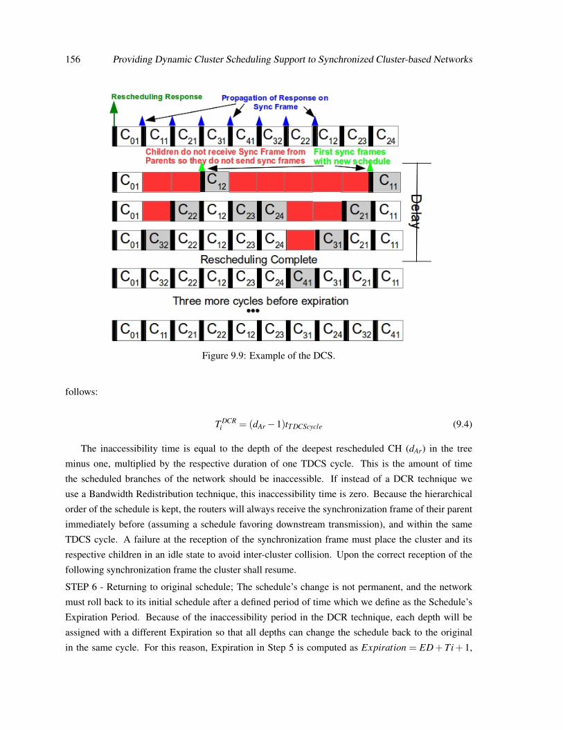
156 Providing Dynamic Cluster Scheduling Support to Synchronized Cluster-based Networks
Figure 9.9: Example of the DCS.
follows:
T DCRi = (dAr−1)tT DCScycle (9.4)
The inaccessibility time is equal to the depth of the deepest rescheduled CH (dAr) in the tree
minus one, multiplied by the respective duration of one TDCS cycle. This is the amount of time
the scheduled branches of the network should be inaccessible. If instead of a DCR technique we
use a Bandwidth Redistribution technique, this inaccessibility time is zero. Because the hierarchical
order of the schedule is kept, the routers will always receive the synchronization frame of their parent
immediately before (assuming a schedule favoring downstream transmission), and within the same
TDCS cycle. A failure at the reception of the synchronization frame must place the cluster and its
respective children in an idle state to avoid inter-cluster collision. Upon the correct reception of the
following synchronization frame the cluster shall resume.
STEP 6 - Returning to original schedule; The schedule’s change is not permanent, and the network
must roll back to its initial schedule after a defined period of time which we define as the Schedule’s
Expiration Period. Because of the inaccessibility period in the DCR technique, each depth will be
assigned with a different Expiration so that all depths can change the schedule back to the original
in the same cycle. For this reason, Expiration in Step 5 is computed as Expiration = ED+Ti+ 1,

9.5 Instantiating DCS in IEEE 802.15.4/ZigBee 157
where ED is the schedule’s expiration deadline that is application defined (DCS_Exp_Deadline) and
can be computed from the amount of data to be received, Ti the inaccessibility time. Each CH will
later compute its own Expiration by subtracting their depth in the tree. By following this rule, every
CH can easily compute when the current schedule expires, just by counting the number of TDCS
cycles since their first synchronization frame after the reschedule. For the case of a DBR technique,
expiration will be always equal to the ED, since the inaccessibility time remains equal to zero. The
CHs should activate a counter at the first synchronization frame sent with the new schedule. From this
point on, each CH keeps track of the current number of synchronization frames sent by it. When this
number is equal to the assigned Expiration value the CH automatically sets its offset to the original
and waits for a synchronization frame from its parent to return to the original schedule. Fig. 9.9
describes how this process should work for the example of S3, after a successful reschedule response.
The delay of three cycles due to inaccessibility is depicted as well as the schedule expiration. The
first TDCS cycle transmits the new offsets within the DCS Response. Each router resets their internal
clock references and waits for a synchronization frame from their parent. C12 and C11 are the first to
receive this and they transmit their synchronization frames with the new schedule, followed by their
child, (C22,C23,C24,C21).
Next, the CHs at depth three do the same until the last CH at depth four (C41) is also rescheduled.
The schedule is kept for three more TDCS cycles and it expires. All the offsets return to the original
schedule in only one TDCS cycle. As observed, the network inaccessibility time is bounded and return
to the original schedule is done without much complexity.
Considering energy-efficiency, only the node which makes the DCS Request, and eventually the
CHs routing that message, spend an extra quantity of energy, which is equivalent to the transmission
of one short data frame, eventually retransmitted in the case of a failure. The setup of the network with
the new offsets uses the payload of the synchronization frames that must be transmitted independently
of DCS. Thus, it is clear that communications generated by our mechanism, will never lead to energy
depletion among the nodes.
9.5 Instantiating DCS in IEEE 802.15.4/ZigBee
The PAN-Coordinator is responsible for receiving the new schedule request from the other cluster-
heads and computing the new schedule as described before. A new module was devised to be inte-
grated above the network layer of ZigBee (Figure 9.10), at the Application Support Layer. This new
module, DCS, is responsible for managing the DCS mechanism, in regards to the beacon payload
creation (for propagating offset information), computing and changing the offset information for the
lower layers, and computing the schedules and corresponding expiration.

158 Providing Dynamic Cluster Scheduling Support to Synchronized Cluster-based Networks
Figure 9.10: DCS ZigBee Implementation.
At network setup time, the TDCS algorithm is applied to the the tree, setting up the base schedule.
As the nodes gather data, they can direct streaming requests at the PAN Coordinator. The PAN-
Coordinator will evaluate these requests according to what is described in Step 3 of Section 9.4.3. If
the result is positive, it will compute the new schedule and setup the Rescheduling Response to be
placed in the IEEE 802.15.4 Beacon Payload. The next Beacon frame will carry this information.
As Beacons are transmitted between the several clusters, the new schedule information is propagated
among the tree and all the nodes will know a DCS Rescheduling is occurring just by parsing the re-
ceived Beacon. This is important since in the next BI, many nodes will fail to receive a Beacon from
their parent, due to the inaccessibility time described in Step 4 of the DCS Communication Protocol.
This will be specially visible in the deepest nodes of the rescheduled branch. If no information con-
cerning the status of the process was propagated, the nodes could assume they had lost their parent,
receiving a SYNC-LOSS.indication from the respective MAC layer, and would try an Association
procedure to another potential parent. By knowing this in advance, they can disable this process for
(Depth−1)∗BI amount of time, which is the maximum time the rescheduling should take per Depth,
after which, the Device will re-enable the re-association procedure after the SYNC-LOSS.
Upon reception of their parent’s Beacon, the ZigBee Cluster-Heads, will search for their address
among the Rescheduling information at the Beacon Payload to learn the new offset. Then, they will
trigger the DCS Module generating a DCS-NEW-SCHEDULE.indication, and set their own Beacon
Payload with the remaining information of the Rescheduling Response to propagate the information
to the children down the tree. Having done this, the DCS Module, will issue a SYNC.request to

9.6 Performance evaluation 159
the Network Layer to resynchronize with the corresponding parent, and after a synchronization an
MLME-START.request.
The MLME-START.request primitive, depends of the rescheduling technique to be used. If a Re-
ordering technique is to be used, then the CH will used a DCS-RESTART-ROUTER.request, with the
new offset information. This new interface is similar the standard NLME-RESTART-ROUTER.request,
except no change is done to the other parameters of the stack. The objective is to simply turn the
routing functionality on. If a Bandwidth reallocation is to be done, then the request will also change
the Superframe Order parameter of the stack to reflect the bandwidth change. The system timers at the
MAC layer, upon reception of this request are automatically updated with the new Superframe Order.
Upon the reception of a Beacon from the parent, the ZigBee Router will automatically resynchronize
and resume its work.
When the DCS Module is triggered, the Schedule Expiration is also computed according to what
is described in Step 6 of Section 9.4.3, and a counter (DCS-Expiration-timer) is triggered with that
value. When this counter expires, the DCS Module automatically repeats the DCS-RESTART process
with the old offset values, returning to the initial values. These are stored in a database, DCS-Initdb,
which contains the initial offset and Superframe Order values. As described, the implementation of
the DCS mechanism does not involve major changes to the protocol. In fact, only a couple of new
interfaces are to be added to the ZigBee NWK implementation to enable the DCS functionalities. One
is triggered upon reception of a new schedule (DCS-RESTART-ROUTER.request) after the regular
parsing of a beacon frame, and another (NLME-RESTART-ROUTER.request) which is a replication of
the standard NLME-START-ROUTER.request. All of the DCS mechanism implementation is taken as
an independent module to the Application Support Layer to avoid imposing substantial changes to the
NWK layer.
9.6 Performance evaluation
9.6.1 Application scenario
Structural Health Monitoring (SHM) and damage identification at the earliest possible stage have been
receiving increasing attention from the scientific community and public authorities [Eco10]. Service
loads, accidental actions and material deterioration may cause damage to the structural systems, re-
sulting in high administrative costs for governments and private owners and, in some situations, loss of
human lives. As such, there is an enormous eagerness to add sensing/actuating capabilities to physical
infrastructures like bridges, tunnels and buildings, turning them into “smart structures” able to detect
and respond to abnormal situations. However, there is still a lack of ready-to-use and off-the-shelf
WSN technologies able to fulfil the most demanding requirements of SHM applications, such as strin-
gent time synchronization of all sensors’ measurements, highly reliable timely measurements and data

160 Providing Dynamic Cluster Scheduling Support to Synchronized Cluster-based Networks
Figure 9.11: SHM System Architecture.
communications. In this line, we designed a prototype system for SHM reported in [SGA+10b] and
[ARL+11], capable of coping with these SHM requirements while supporting network scalability.
This application presents interesting dynamics that could be improved by the use of the DCS mech-
anism. Besides its requirement of tight node synchronization and low latency downstream control, the
application generates a large amount of sensing data that must be handled by the network in an up-
stream direction. These two modes of operation can be supported and see their performance improved
by the use of the DCS mechanism by minimizing both end-to-end delays and overall transmission
time.
Its system architecture was designed to sample in a synchronized fashion multiple accelerometers
placed at different locations in a physical structure and forward this data to a central station (PAN-
Coordinator) for later processing using a IEEE 802.15.4/ZigBee Cluster-Tree network topology. Each
Sensing Node is composed by a TelosB node with a signal acquisition board, with a 24 bits DAC,
attached to a MEMS 3-axis acceleration sensor (Fig. 9.11). The application is thoroughly described
in chapter 5.
The network is setup according to Fig. 9.1 network topology and the Sensing Nodes are spread
into different clusters. In Fig. 9.1, the addresses next to the nodes represent the Cluster-Heads’ ZigBee
NWK addresses. The initial schedule favors downstream communications. This is made so that the
PAN-Coordinator, after setting up all the nodes in the network, is able to start and stop the data
acquisition on all the nodes simultaneously, in one TDCS cycle. This is mandatory for the application

9.6 Performance evaluation 161
Figure 9.12: Experimental DCS Schedules.
so that the results are coherent. If the initial schedule was kept to poll the date from the sensors,
the assessment could last minutes up to several hours, depending on the cluster the stream originated
from.
We aim at changing the network’s TDCS schedule to improve on this behaviour, by (1) reducing
end-to-end latency, eventually allowing for simultaneously data analysis, using the DCR technique
and (2) by accelerating the data transfer from the Sensing Nodes to the PAN-Coordinator using DBR
technique.
9.6.2 Experimental setup
The DCS mechanism was evaluated through simulation and experimentally using our SHM system.
For carrying out the simulation analysis, the DCS mechanism was implemented over the Open-ZB
Zigbee Model [ZA05], and simulated with the OPNET Modeler simulation software. A network
topology like the one shown in Fig. 9.1 with nwkMaxChildren (Cm) = 3, nwkMaxDepth (Dm) = 5,
and nwkMaxRouters (Rm) = 2, was setup and the application layer of the node was set to generate
traffic at a rate correspondent to a sampling rate of 100Hz which is recommended for fine-grained
structural health monitoring [SGA+10b]. For maintaining uniformity along this work, in the analysis

162 Providing Dynamic Cluster Scheduling Support to Synchronized Cluster-based Networks
we always consider stream S3, which originates at router C41 in Figure 9.1 and constitutes the worst-
case for the initial TCDS schedule. Several analysis to evaluate the performance of the two techniques
were carried out, with a special attention to two metrics: end-to-end delays and overall stream transmit
duration.
To carry out the experimental validation over the SHM application, the DCS module was imple-
mented in TinyOS over the Open-ZB IEEE 802.15.4/ZigBee stack [CKSA07]. A ZigBee network with
12 TelosB motes was setup in a configuration replicating the one depicted in Fig. 9.1, using BO=8 and
SO=4, with one PAN-Coordinator connected to a PC through a USB connection, and nine Routers
each forming their own cluster. Two Sensing Nodes (End Devices) were associated to the Router at
Depth 4 (address 0x0004) to generate sensing data for later retrieval. To reduce costs, the Sensing
Nodes were used without the accelerometer modules. Instead, timers at the application layer were
used to emulate real SHM traffic at different sampling rates. Both DCS techniques were implemented
and tested to validate our work, although the most important technique for this specific SHM applica-
tion is the DBR, which as shown before can greatly reduce the overall stream transmission time. A
base scenario, without any schedule improvement, was also setup to measure the improvement.
9.6.3 Performance results
9.6.3.1 End-to-end Delay Analysis
To understand the impact of the first technique we did one hundred simulation runs, 10 minutes each,
of the network with different BO settings (from BO = 8 up to BO = 12), simulating a larger network,
with the initial scheduling and using the cluster re-ordering technique. The maximum end-to-end
delays were measured for packets transmitted from a Sensing Node associated to Router 0x0004,
at Depth 4, (S3 in Fig. 9.1), to the PAN-Coordinator, with no other traffic on the network. This
transmission is the worst-case for the initial TDCS schedule. In the simulation platform, frame size
was set to 800 bits, and Packet Inter-arrival Time was set to 0,06 seconds to emulate the arrival of
Sensing Data at the Sensing Node’s serial port (this was verified experimentally).
Fig. 9.13, shows the simulation maximum end-to-end delay results for the different BO using the
DCR technique. Superframe order is fixed to SO = 4 for the case of the results in the left. Notice the
decrease on the delay achieved by simply re-ordering the schedule. We can achieve a reduction in the
end-to-end delays in the order of 13 seconds for BO = 8 and even several minutes as the BO increases
with the size of the network, reaching 4 minutes for the case of BO = 12, to approximately one second.
The end-to-end delays with DCR remain constant despite the different BO settings. This is expected
since although the network increases, the transmission of a packet is completed in only one BO cycle.
Since the Bandwidth of the routers is also the same, the end-to-end delay should remain constant and
thus independent of the network size.

9.6 Performance evaluation 163
Figure 9.13: Stream end-to-end delays - simulation.
To understand the impact of the Bandwidth Reallocation technique (DBR), on the end-to-end
delay, the initial schedule’s ordering was maintained, and BO increased to 10. As the available band-
width of the Superframe increased, it was distributed using DBR among the Routers involved on the
stream, changing from SO=4 up to SO=7. Fig. 9.13 on the right, presents the results for S3 in Fig. 9.1
concerning end-to-end delay.
There is a slight but not significant decrease of the end-to-end delay as the SO is increased. Since
the Routers increase their SO, the unused part of the Superframe was reduced and thus there is a
better use of the Superframe bandwidth. This reduces the time the packet must remain in the queue at
each router, waiting for the next Superframe to be transmitted to the parent, thus slightly reducing the
overall end-to-end delay. This is visible in the figure in the right showing how the average queuing
delay decreases as the SO increases. In comparison, the DCR technique presents a much higher impact
on the end-to-end delay as expected, decreasing for the case of BO/SO = 10/5, the delay from 60.95
to 1.97 seconds, a decrease of 96.7%. In fact, for its worst case of BO/SO = 10/7, it still represents a
decrease of 82.14% concerning the DBR technique.
There is however, a slight increase in the end-to-end delay when using the DBR+DCR techniques
as the SO increases. Although, there is a re-ordering of the schedule according favouring upstream
traffic, and a redistribution of the unused bandwidth, the increase in SO implies a larger time a packet
must wait in queue at each router, waiting to be transmitted to the parent, in comparison to the cases
with lower SO. Using the DBR technique is thus not recommended.

164 Providing Dynamic Cluster Scheduling Support to Synchronized Cluster-based Networks
Figure 9.14: Stream End-to-end Delays - Experimental and Simulation.
Fig. 9.14 shows the comparison between simulation and experimental results. As observed, the
behaviour previously observed in simulation is replicated in the experimental evaluation with minor
differences. However for the base schedule, experimental delay was slightly different. This has to
do with the different duration of the Beacon Order on the experimental platforms, which is of 3.75
seconds instead of the theoretical 3.932 seconds, due to the lower timer granularity.
A Daintree Networks 2400E Sensor Network Analyzer [Dai15b] was used to log all the commu-
nications during the experimental evaluation. Fig. 9.15, shows its log after a successful reschedule
response. Part of the output related to the network setup and DCS communication was omitted to save
space, but can be seen in [SPT13b]. The beacons from the PAN Coordinator are signaled with a red
arrow. When all the Routers receive their new offset information in the DCS Reschedule Response
message, they immediately stop sending beacons and wait for their parent’s beacon to synchronize to
it. The first beacon comes from the PAN Coordinator which maintains its period. Next, Routers at
Depth one are the firsts to synchronize to it using the new offsets. Notice the Packet Analyzer time
stamp, showing the new relative offsets. Now that the Depth one Routers transmitted their beacons,
the next level ones (Depth two) can also synchronize. The process continues until the all the Routers
are synchronized. At this point, the Sensing Nodes (0x0007 in the example) start transmitting data
which will be forwarded until it reaches the sink.
9.6.3.2 Stream Overall Transmission Time
Like previously mentioned, minimizing the overall transmission time is quite important, in this SHM
application, where large amounts of data must be transmitted in the less amount of time possible.
To analyze this metric, in the simulation platform we generated scenarios with different volumes of
sensing data, corresponding to short 10 and 30 seconds runs and runs with 1, 5, 10 and 30 minutes, in

9.6 Performance evaluation 165
Figure 9.15: Output from the packet analyzer showing the DCR technique.

166 Providing Dynamic Cluster Scheduling Support to Synchronized Cluster-based Networks
Figure 9.16: Stream transmit duration.
the SHM system. Those values were also tested in the experimental platform. During this time there
was no other traffic in the network, as to not interfere with the experiment.
Fig. 9.16 shows the simulation and experimental results of the transmission time for sampling
durations of 30 seconds, 60 seconds and 5 minutes using the DCR and DBR techniques for SO=4
and SO=5 in regard to the base schedule. As shown, the DBR technique presents the best result in
decreasing the overall transmission time, representing a decrease close to 50%, as expected when the
available bandwidth is doubled on the Routers, to SO = 5. For the case of 1 minute of sampling time,
using the DBR technique alone reduced the overall transmission time from nine minutes to 4 and a
half minutes, a decrease of 49%.
Interestingly, the DCR technique also decreases the overall transmission time, but not in a signifi-
cant way. It decreases it about 14 seconds for this particular case of BO=8, and it is constant for every
SO setting, independently of the amount of data to be transmitted. However, this small difference
should not be neglected. For larger BO, the impact of this increases as shown in Fig. 9.16 in the right,
reaching 8 minutes for BO=13. This happens because of the impact of the reduced end-to-end delay
at the beginning of the transmission, due to the re-ordering of the clusters’ schedule. Because of this,
the transmission will end sooner. As the BO increases, the impact of this is higher since the duration
of the TDCS cycle also increases.
Experimentally, concerning the DBR technique, results show a reduction on the overall transmis-
sion time in the order of 49%, again quite close to simulation results, while further reductions can be
achieved by increasing the SO per cluster. Concerning the network inaccessibility time, as predicted,
it was bounded to three TDCS cycles, which is the time it takes for the whole network to resynchro-
nize with the new schedule. This can be confirmed in the Packet Analyzer output files available in
[SPT13b].
Starting with the DBR technique, the most important parts of the log are highlighted in Figure 9.17
and commented bellow.
A few packets were omitted for space reasons to simplify the reading. This figure shows the use of

9.7 Final Remarks 167
the DBR technique to reduce the overall stream transmission time. Beacons from the PAN Coordinator
are signaled with a red arrow.
At network setup time, the nodes associate (1) and the TDCS algorithm assigns each cluster an
offset (2), assuming a the initial schedule favoring downstream communication, thus improving the
control over the application during the sampling period. This information is sent in a Data Message
(blue Data Message inside rectangle 2). The application is configured and started (3), and the base
schedule can be seen. Upon completion of the data acquisition task, the application pools the nodes
for data. The first Sensing Node to be pooled, wishes to initiate upstream data communication and
triggers the DCS mechanism (4) with a DCS Request. This request is forward by the routers until
it is delivered to the PAN-Coordinator. Two Data Messages with DCS Request can be seen being
forwarded. The relationship between addresses and the logical topology is shown in Figure 9.1.
Upon arrival, the PAN Coordinator computes the new schedule and sends to the network a DCS
Reschedule Message which is disseminated within the payload of the beacon frame throughout all the
network (5). The new schedule is immediately adopted as shown in (6), and a change on the SO is
noticeable on the Beacon frame description and on the sniffer timestamps.
9.7 Final Remarks
Changing the resource allocation of a Cluster-based WSN on-the-fly, without imposing long inacces-
sibility times, represented a major challenge, hindering the deployment of many WSN applications.
With this work, we propose a solution to this problem, enabling networks to self-adapt to changing
traffic flows, improving the QoS by redistributing the available bandwidth and minimizing latency,
assuming a given schedule based on a time-division strategy.
We presented two techniques achieving a reduction of the end-to-end delay from a leaf node to the
sink of 93%, and a decrease of the overall data transmit period of 50% although a higher impact can
be achieved with other network settings. Importantly, our methodology was applied to a real-world
WSN-based Structural Health Monitoring system, showing that it can be easily implemented under
the IEEE802.15.4/ZigBee set of protocols with minor add-ons and can run in general purpose WSN
platforms such as the TelosB motes.
In the near future, we aim at deploying the SHM system fitted with DCS in the field, supporting
civil engineers that must carry out professional structural health monitoring work. We are also aiming
at providing support for conflicting traffic flows in the network.
In the next chapter, this thesis works towards the design of an online and cross-layer mechanism to
manage the different QoS properties already mentioned so far in the context of IEEE 802.15.4/ZigBee
networks.
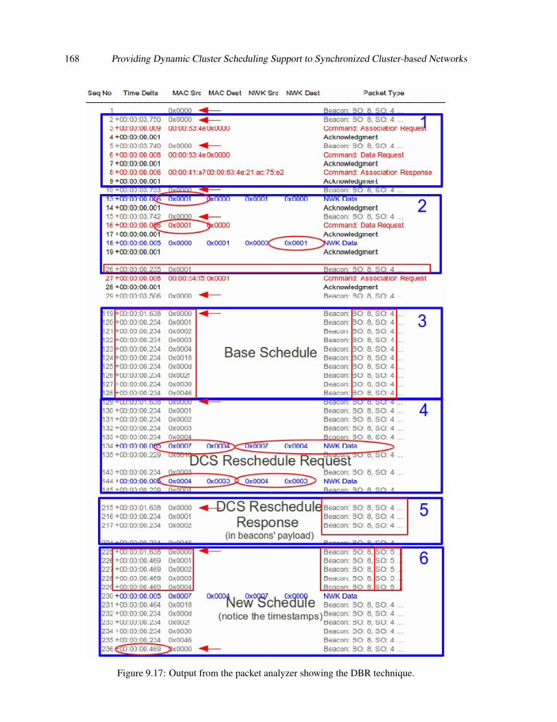
168 Providing Dynamic Cluster Scheduling Support to Synchronized Cluster-based Networks
Figure 9.17: Output from the packet analyzer showing the DBR technique.

Chapter 10
Adding Online Cross-layer QoS Controlto ZigBee Cluster-based Networks
This Chapter presents a cross-layer QoS management framework for ZigBee cluster-tree networks.
The proposed framework carries out an on-line control of a set of parameters ranging from the MAC
sub-layer to the network layer, improving the successful transmission probability and minimizing the
memory requirements and queuing delays through an efficient bandwidth allocation at the network
clusters. Through extensive simulations in a real datacenter monitoring application scenario, we show
that the proposed framework improves the successful transmission probability by 10%, and reduces
the end-to-end delay by 94%.
10.1 Introduction
Wireless Sensor Network (WSN) infrastructures show a great potential to address various challenges
posed by the large-scale energy consumption, cooling, and operational needs of large data centers,
by providing a sensor layer to monitor parameters such as temperature, humidity, airflow and power
consumption per server. Existing data centers consume around 50% of the supplied energy in cooling
related actions [Koo11]. A WSN infrastructure can enable more precise and efficient control of the
datacenter’s equipment and may reduce the cooling cost.
However, WSN applications have different Quality of Service (QoS) requirements [RC08], par-
ticularly in what concerns timeliness. Structured logical topologies such as cluster-trees are generally
used to address these QoS requirements ([APK04], [GXX07], [PA07]). They provide deterministic
behavior instead of flat mesh-like topologies, where timeliness is not always guaranteed. The ZigBee
[ZA05] standard has proposed a cluster tree network topology to address different QoS requirements
of heterogeneous applications and support synchronization and predictability through a hierarchical
169

170 Adding Online Cross-layer QoS Control to ZigBee Cluster-based Networks
network structure. However, this topology is not directly adaptable due to implementation and flex-
ibility problems. Few solutions have already been proposed to address these problems ([KCAT08],
[KANS06], [SPT14]) however, to the best of our best knowledge, no attempt has been made to inte-
grate them in one framework capable of supporting online and dynamic cross-layer QoS management
mechanisms for cluster-tree networks ([SEN14], [PTL+15]). This framework should be able to allo-
cate network resources online and increase the network flexibility in terms of latency and bandwidth
utilization, since these networks usually rely on a static cluster schedule. It should also adapt its MAC
sub-layer to different traffic priority classes using a cross-layer approach. This would result in a frame-
work capable of addressing not only the timeliness, but also other QoS aspects such as robustness, by
providing the network infrastructure with self-adapting capabilities, and energy-efficiency, by provid-
ing traffic differentiation at the MAC sub-layer, improving the successful transmission probability to
selected nodes, for instance, while relying upon the underlying cluster duty-cycling provided by the
IEEE 802.15.4 beacon enabled mode.
This work presents a cross-layer QoS management framework that provides automatic and on-
line control of two QoS mechanisms for ZigBee cluster-tree networks. At the Medium Access Control
(MAC) level, we improve the successful transmission probability of a tagged node, by carefully tuning
the MAC parameters. The successful transmission probability is calculated by the fraction between
the number of successfully acknowledged frames and the traffic generated at the application layer. At
the network level, we reduce the queuing delays and memory requirements per node by carrying out an
on-line efficient allocation of the available bandwidth for each cluster. This results in the elimination
of bottlenecks in the network infrastructure, achieving a clear improvement in the end-to-end latency
of the application. This work relies on two previously proposed and validated mechanisms, the Traffic
Differentiation Mechanism (TRADIF) proposed in [KANS06] and the Dynamic Cluster Scheduling
(DCS) proposed in [SPT14]. We extended the TRADIF mechanism to provide control of multiple
nodes in the same cluster. An online performance evaluation mechanism is managed by a cross-
layer Traffic Efficiency Control Module (TECM), which enables the necessary QoS mechanism where
and when needed. The TECM also supports a mechanism to enable scalable and synchronized data
acquisition in multiple clusters (SSYNC) as proposed in [TKD+13]. However, this mechanism must
be enabled on demand. To regulate access to the beacon payload from different modules, a Beacon
Payload Management module (BPM) is also proposed in this work.
We further validate and demonstrate the proposed mechanisms through simulations in a datacenter
monitoring application scenario, which will be deployed in a new large-scale datacenter infrastructure
in Portugal [SEN14], using WSN as a sensing infrastructure to collect power and environmental data
with high resolution and timing constraints. The simulation results show that the traffic rates are
adjusted automatically by using TECM and by triggering DCS effectively. This results in a significant
decrease of memory requirements, minimizing queuing overflow and end-to-end average latencies by
90%. The results also show the possibility of improving the successful transmission probability of

10.2 Related Work 171
higher priority nodes by 8% due to reduction in retransmissions, thus reducing the average energy
consumption. Moreover, we conclude that the efficient pairing of TECM with DCS achieves a more
efficient distribution of bandwidth than that of DCS only. This makes it possible for the network to
accommodate higher traffic rates that would not be feasible otherwise.
10.2 Related Work
In this section, we provide a brief overview of QoS in IEEE 802.15.4/ZigBee networks. This overview
is classified into the following two groups:
10.2.1 QoS improvements to the IEEE 802.15.4/ZigBee standard
Several research efforts focus on improving the performance of IEEE 802.15.4 slotted CSMA/CA pro-
tocol in terms of delay and reliability of time-critical events. A thorough review of such mechanisms
is available in Section 7.2 of this thesis. Concerning the ZigBee protocol, we further present the most
prominent proposals.
The above work focused on traffic differentiation over the IEEE 802.15.4 networks, however, none
of this work discussed on-the-fly alteration and implementation of different parameters. Considering
that traffic and network performance may change during the network lifetime, it is important that the
parameter tuning may be carried out periodically, adjusting to current network performance. This
may avoid unnecessarily decrease in the performance of lower priority traffic. Concerning the net-
work layer, general synchronized cluster-tree topologies tend to suffer from four technical challenges:
(1) how to schedule the transmissions of different neighboring clusters avoiding interference, (2) how
to predict the performance limits to correctly allocate resources, (3) how to change the resource allo-
cation of the cluster-tree on-the-fly, and (4) the lack of available and functional implementations over
standard WSN technologies, such as the IEEE 802.15.4/ZigBee protocols. This is particularly true for
IEEE 802.15.4/ZigBee protocols, which support the cluster-tree network topology but do not provide
a clear description of implementation problems including beacon collision problems. In [IT06], the
IEEE 802.15.4b proposed some basic approaches to solve the aforementioned problems: the beacon-
only period approach and the time division approach. Few other approaches targeted the scheduling of
ZigBee cluster-tree networks. The work in [PT08] introduced the minimum delay beacon scheduling
problem, however this work only addressed the latency problem by assuming the use of GTS slots for
converge cast, and do not address the bandwidth problem. In [KCAT08], the authors proposed a Time
Division Cluster Schedule (TDCS) algorithm for IEEE 802.15.4/ZigBee networks and implemented
it in the Open-ZB stack [CKSA07]. This algorithm used a time-division approach and worked by
assigning a different time offset to each cluster. The implementation of this work is available to the
TinyOS and WSN communities [Tin15], through the Open-ZB [OZ15] framework. This work is of

172 Adding Online Cross-layer QoS Control to ZigBee Cluster-based Networks
great importance since it solves the beacon scheduling issues for ZigBee cluster-tree networks. Other
approaches, such as [BW07] and [MdPSP] followed a similar approach to [KCAT08] for mesh net-
works. The work in [JKS+10] addressed the problem of predicting resource needs by modeling the
performance limits of ZigBee cluster-tree networks using GTS flows. In another work, the authors
extended the latter by computing the optimal schedule for several GTS data flows [HJ10]. Recently,
[DFPD12] followed a similar approach to [PT08] proposing two heuristics to reduce the complexity
of the otherwise NP-complete problem. Although the usage of GTS guarantees real-time performance
within the IEEE802.15.4/ZigBee standards, the number of available GTS slots and their bandwidth
is limited. The authors of [HPH+12] tried to improve the GTS bandwidth utilization by borrowing it
from the neighboring nodes.
The above research efforts compute a static schedule based on periodic traffic assumptions, which
remain active throughout the network lifetime. They follow a purely theoretical approach, lacking a
clear description on how to implement such mechanisms on ZigBee cluster-tree networks. In [SPT14],
the authors presented a much simpler and low complexity DCS algorithm to satisfy bandwidth and
delay requirements by rescheduling the clusters. It proposes two mechanisms: (1) carries out a
rescheduling of the clusters ordering in the TDCS cycle aiming at minimizing end-to-end delays, and
(2) rearranges the bandwidth allocation for the clusters involved in a stream, increases its bandwidth
and decreases the overall data transmission time, and minimizes the queuing size and delay. Both
techniques can be used together, or separately. The DCS algorithm was validated through simulations
and implemented over TinyOS in real WSN platforms. Although each mechanism can be triggered
on-the-fly, the user must specify a threshold based on a maximum predefined amount of traffic. This
might be hard to correctly select without a simulation or experimental approach. Furthermore, to
avoid increased complexity, the algorithm increases the bandwidth among all the clusters in the traffic
stream which may not always be necessary and may create inefficiency. Nevertheless, we believe this
is the most simple and practical approach and can improve the performance even further.
10.2.2 Online and cross-layer QoS proposals
As discussed above, most of proposed research efforts do not encompass an online mechanism to ap-
ply the necessary changes as the network performance decreases, and exactly where needed. Instead,
they usually rely on the user to enable these services through application mode changes according to a
set of assumptions usually obtained from simulation scenarios, and in most cases without performance
feedback from the network. This suboptimal approach usually leads to an unnecessary decrease in the
performance of low priority traffic at the MAC level, and also, to a waste of precious bandwidth re-
sources at the network level, as traffic varies through time. Moreover, these approaches rely on the
expertise of the user to control complex mechanisms, for instance, setting MAC parameters. Clearly

10.3 On the Supported QoS Mechanisms 173
this is a big impediment for a democratization of these networks, unnecessarily increasing their com-
plexity, as most users do not hold the knowledge to fine tune these parameters. Since the traffic
conditions may change, these settings must be updated throughout the entire network lifetime in many
cases. Furthermore, as the QoS provisioning is not a one layer specific issue, the QoS management
becomes a daunting task as the number of layers at the communication stack increases. The network
layer performance for instance, is tightly coupled with the MAC sub-layer for efficient resource al-
location. This resource allocation requires a cross-layer mechanism that must be able to address the
QoS problems at MAC and network layers.
Cross-layer strategies have already been proposed in the literature ([YIE11], [MJR11]) as an ef-
ficient way of solving many issues in WSNs. Most of these strategies focused on tuning parameters
in different layers of the stack. Unfortunately, existing proposals which target QoS related issues, are
either not compliant with ZigBee [SLA12] or do not address the particular case of ZigBee cluster-
tree networks such as in [NY11]. In our proposal, by joining TRADIF and DCS, coupled with the
proposed TECM online management capabilities, we achieve a cross-layer online QoS management
service for ZigBee cluster-tree networks. We further show how the successful transmission probabil-
ity of a higher priority best-effort traffic class can be dynamically improved through TECM/TRADIF
and how the overall end-to-end delay can be reduced through TECM/DCS, by tuning MAC sub-layer
parameters and the clusters duty-cycle respectively. Furthermore, this work results in a more efficient
usage of energy and memory because of less retransmission attempts and reduced queue size.
10.3 On the Supported QoS Mechanisms
In this Section we present an overview of the QoS mechanisms supported by our proposal. The
TRADIF mechanism aims at achieving traffic differentiation at the MAC sub-layer, while the Dynamic
Cluster Scheduling proposal works at the network layer, by improving the clusters’ scheduling.
10.3.1 TRADIF
TRADIF is a traffic differentiation mechanism, fully backward compatible with the IEEE 802.15.4
standard, which works by tuning a few MAC parameters. This mechanism is implemented in OP-
NET Open-ZB IEEE 802.15.4/ZigBee simulation model [OZ15]. It is also validated over the ERIKA
[Evi15] real-time operating system in [SBAK10], using real WSN platforms and presented in Chap-
ter 7 of this thesis.
TRADIF differentiates traffic classes previously defined at network setup time, by tuning different
MAC parameter values. Originally, these settings remain active regardless of the network perfor-
mance. While simulation could be carried out to assess the correct settings, there are several impli-
cations: (1) it is assumed that the user has enough expertise to carry out this task; (2) because the

174 Adding Online Cross-layer QoS Control to ZigBee Cluster-based Networks
Figure 10.1: TECM timing diagram
settings remain active throughout the network lifetime, even if no traffic arrives from a higher priority
class, the lower priority will still experience an unnecessary service downgrade.
We address the above problems by adding intelligence to the triggering of TRADIF. Performance
indicators (successful transmission probability and the ratio of retransmissions) are used to trigger the
proposed mechanism only if a service decrease for a high priority node is noticed. This is independent
from the user, as it no longer chooses the parameter settings. Instead, TRADIF will change the respec-
tive MAC parameters in successive steps, until the performance indicator reaches an acceptable level.
For instance, since the highest impact on the successful transmission probability metric is caused by
changing CW, a decrease of service at a higher priority class will trigger TRADIF which will auto-
matically increase the CW value of the lower priority classes to the next value. This process will be
repeated until there is no noticeable degradation. To extend the capabilities of TRADIF at network
level, a simple communication protocol is used to enable an interface between the TRADIF modules
at different nodes. This enables a high priority node to ask for an increase of the CW of remaining
nodes in the cluster, thus improving its success probability. Figure 10.1 presents a timing diagram of
the communication protocol, when TECM triggers TRADIF to improve the success probability of a
high priority node.
Upon request, the TRADIF module must reduce the successful transmission probability of the
lower priority nodes which compete in the same cluster. It then sends a TRADIF Request to its parent
with three fields. The first field in Figure 3 indicates the kind of nodes it is targeting (high (HP) or
low priority (LP)), the second indicates the metric to be affected (successful transmission probability

10.3 On the Supported QoS Mechanisms 175
or throughput) and the third indicates the direction (increase or decrease). The request is received by
the parent’s TECM module and the contents of the request are forwarded as a TECM message to the
Beacon Payload Manager module (BPM). This TECM message is incorporated in the beacon payload,
which is received by all the cluster’s nodes. Upon reception, the BPM forwards the payload to TECM,
which will trigger TRADIF-SERVICE. TRADIF will then increment CW (of low priority nodes). If
the higher priority node’s performance does not improve, the process will be repeated.
10.3.2 Dynamic Cluster Scheduling
With TDCS [KCAT08] it is possible to find the best schedule for the routers active periods in order
to avoid interference, and to support most of the network bandwidth requirements. However, the
schedule is done at network setup time, which assumes a static network that will remain unchanged.
Thus, the choice of TDCS schedule has a strong impact in the end-to-end delays and on the available
bandwidth for each cluster throughout the network lifetime.
The DCS reacts to different data flow changes on-the-fly, while simultaneously minimizing the net-
work inaccessibility time using two techniques as proposed in [SPT14]: (1) DCS Cluster Re-ordering
(DCR), which re-orders the clusters’ active periods to favor one set of streams and reduces end-to-end
delays, and (2) DCS Bandwidth Re-allocation (DBR), which tunes the size of the clusters’ duration
and increases the bandwidth of the clusters serving a specific stream, while decreasing others band-
width if needed. The DCR consists of a rescheduling of the clusters order in the TDCS cycle, aiming
at minimizing end-to-end delays, while the second technique consists of rearranging the bandwidth
allocation for the clusters involved in a stream, to increase its bandwidth and decrease the overall time
for a data transmission, minimizing the queuing size and delay.
There is however a room for improvement in DCS. For instance, in DCS a node triggers the
mechanism if the size of the stream of data which is to be transmitted is larger than a threshold.
However, specifying this threshold is not easy and usually simulation must be done to choose this
value. In DBR, on the other hand, the mechanism distributes a fixed amount of bandwidth throughout
all the nodes in a stream in an equal fashion, without any added benefit, wasting precious bandwidth
that may be required by other nodes. Often, only the nodes at the lower depths need extra bandwidth
due to the higher concentration of traffic at nodes near the sink (assuming sink is at the root). In fact,
even when the others at higher depths need bandwidth, it is not always in an equal amount.
In this work, by joining DCS with TECM we can carry out a better and fairer redistribution of
the bandwidth in an on-the-fly fashion. TECM relies on a performance indicator at each node which
accounts for the input/output traffic ratio as well as the queue size. If the indicator drops below a
threshold, TECM will trigger the DCS-DBR mechanism to increase the available bandwidth exactly
where needed, improving the efficiency of the mechanism. To do this, only a change to the triggering
mechanism is required. This process is discussed in detail in the next section.

176 Adding Online Cross-layer QoS Control to ZigBee Cluster-based Networks
10.4 Traffic Efficiency Control Mechanism
In this Section we elaborate on the TECM mechanism. We present its system architecture, the perfor-
mance metrics used to support the online netowork performance monitoring, and its algorithms. We
also propose a mechanism to manage the access to the beacon payload, considering many of the QoS
mechanisms use this method to convey their messages in the network.
10.4.1 TECM Architecture
The TECM consists of an online cross-layer module aiming at improving the QoS in ZigBee cluster-
tree networks. It can improve the cluster scheduling, reduce end-to-end delays and queuing sizes
using DCS, and improve the successful transmission probability for a higher priority traffic class using
TRADIF. It relies on an online algorithm that periodically assesses the performance of the network
and triggers the necessary QoS mechanisms. Figure 10.2 shows the proposed system architecture.
The figure shows how the TECM module is wired into the IEEE 802.15.4/ZigBee stack and its most
relevant services and Service Access Points (SAPs). The top three layers of the communication stack
are implemented by the official TinyOS 2.x IEEE 802.15.4/ZigBee stack [Tind].
The Application Layer (APL) is stacked at the top and connects to an example of a Datacenter
Monitoring Application. The Application Support Sublayer (APS) provides the interface between
the APL and the Network Layer (NWK) of the ZigBee communication stack through the NLDE and
NLME ZigBee Service Access Points (SAPs). The DCS-SAP is also shown since it supports the
DCS mechanism as described in [SPT14]. The NWK also supports several network management ser-
vice modules such as DCS, TDCS, BPM and SSYNC. The TDCS module is only implemented at
the routers and the Coordinator. It is responsible for the scheduling negotiation and is triggered at
network setup, upon successful association by the application. The SSYNC module, supports the ap-
plication network wide synchronized data acquisition as described in [TKD+13], enabling all clusters
to synchronize to any moment in time. By doing this, we can ensure that despite the clusters’ different
offsets between them, all can wake up or, for instance, sample a sensor simultaneously. This is of
course supported by the underlying IEEE 802.15.4 beacon-enabled mode.
The DCS module is responsible for the dynamic rescheduling of each cluster. All the three kinds
of nodes (ZC, ZR and End Devices) implement the service. The necessary interfaces to the MAC
sub-layer are done through the regular IEEE 802.15.4 service access points. Within NWK in the fig-
ure, a dotted box shows a set of files of the communication stack implementation which were changed
to support the necessary TECM packet counters for the performance assessment. At the MAC sub-
layer, the TRADIF is implemented according to [SBAK10], however, an extra set of interfaces was
introduced to enable control of the CSMA/CA parameters by TECM. Also a few interfaces were con-
nected to different modules of the communication stack to retrieve information from the implemented

10.4 Traffic Efficiency Control Mechanism 177
Figure 10.2: TECM system architecture
packet counters. Again, these modules are shown in dotted boxes. These interfaces are part of the
MLTEC-SAP.
The cross-layer module, TECM, manages the DCS and the TRADIF modules and uses different
SAPs to interface each layer. In addition, it periodically pools through MLTEC-SAP and NLTEC-SAP
a set of counters at the NWK and MAC layer to carry out the performance analysis. After processing
a set of algorithms, it can trigger changes to the network scheduling and MAC parameters using the
DCS or TRADIF modules respectively. The TECM SAPs implement a set of interfaces: (1) GET,
which is called from TECM to receive the value of an attribute, (2) SET, which is used to set an
attribute, and (3) RESET, which is always called at the beginning or if an issue is detected, similarly
to the way the IEEE 802.15.4 and ZigBee SAPs are implemented.
The communication with the TECM module by the Application Layer is done using the TECM-
SAP set of interfaces. These include: A TECM-control interface to control the starting and stopping

178 Adding Online Cross-layer QoS Control to ZigBee Cluster-based Networks
of the TECM module at any time; the TECM-setmode, to choose the TECM mode of operation (auto
or fixed-rate), and TECM-setup, to program the different TECM parameters as follow:
TECM-setup (sampling window size, enabled modules, thresholds);
where the sampling window size sets the period of the TECM performance analysis, enabled modules
field informs the TECM module of which services are available (DCS and TRADIF by default), and
the threshold field is used to specify the performance thresholds for each module. If none are specified,
TECM will use a default setup.
TECM provides two modes of operation: auto-rate and fixed-rate. In the auto-rate mode, the
TECM module will try to maximize the application traffic rate, by increasing it to a pre-defined steps
established by the TECM-setmode interface, and by changing the network setup as necessary to ac-
commodate the increase. This can be useful when there is no specific constraint concerning the traffic
rate, but the objective is to optimize the use of the network resources, while keeping an acceptable per-
formance. In the fixed-rate mode, the user defines at any point a traffic rate that should be maintained.
The TECM module will trigger the DCS and TRADIF mechanisms as needed to guarantee an accept-
able network performance. If at any point the TECM module is no longer capable of maintaining an
acceptable network performance, due to reaching the maximum available bandwidth for that partic-
ular cluster, it will inform the application layer through the APLTEC-SAP, and the user can chose
its action. This mode is also able to detect a reduction in the traffic rate, and reduce the previously
assigned bandwidth if it is no longer required.
10.4.2 Beacon Payload Management Module
The Beacon Payload Management Module (BPM) module in Figure 10.3 consists of an interface layer
for beacon processing between the NWK, the several APS service modules and the APL. Its objective
is twofold: to manage the received beacon payload and deliver it to the corresponding module (DCS,
SSYNC, or TECM) or the APL, and to manage the concurrency from different modules which try
to access and modify the beacon payload before sending it to NWK layer. To avoid long processing
delays at beacon reception, only one module at a time is allowed to access the beacon payload.
Thus, each module delivers the content to the BPM module which places it within a FIFO queue.
When ready, it builds the new beacon payload structure and signals the NWK layer.
The resulting beacon payload is illustrated in Figure 10.3, where BPM message type field identifies
the payload contents, the Module ID field identifies the information being integrated in the beacon
payload, the Size field identifies the length of the payload, and finally, the Module Payload identifies
the beacon contents.

10.4 Traffic Efficiency Control Mechanism 179
Figure 10.3: BPM module description
10.4.3 Performance Indicators
TECM periodically carries out a performance analysis based on a set of indicators at each node, every
i-th interval. It relies on two performance indicators, which assesses the network QoS concerning
bandwidth requirements and successful transmission probability.
The first performance indicator denoted by di represents the relationship between incoming and
outgoing traffic, which gives a measurement of the bandwidth requirements of a node. This perfor-
mance indicator can be computed as a balance (adjusted by a) of two terms:
di = accsma
cNWK+(1−a)
ccsma
cqueue(10.1)
where the first term represents the ratio between the number of packets transmitted by Slotted CSMA-
CA algorithm (ccsma) and the number of packets delivered by the NWK (cNWK) and eventually trans-
mitted during a time window. A decrease in this term indicates that not all packets delivered by the
NWK will be transmitted, resulting in an accumulation of packets in the queue. The second part of
the performance indicator concerns the total size of the queue (cqueue) by considering the amount of
packets that will be transmitted at each period. If this performance indicator decreases, it indicates
that the queue is growing. This will result in a cost to di until the outbound/inbound traffic ratio inverts
become higher than one, which indicates that the node is serving a higher amount of packets than the
ones delivered by the NWK, showing that the queue is being emptied.
If the di indicator reaches its maximum of 1, it means the node’s queue is emptied at each active
period, thus no more bandwidth is needed. To smoothen out the result, avoiding sharp transient oscil-
lations that could trigger the mechanism inadvertently, the last result for Di is always considered in an
exponential moving average, where α is used to balance the average, resulting in:
Di = αdi +(1−α)Di−1, i > 0 (10.2)

180 Adding Online Cross-layer QoS Control to ZigBee Cluster-based Networks
The second performance indicator, ti, concerns behavior of the MAC layer concerning successful
transmissions, and it is represented by a balance of two ratios adjusted by b. The first term calcu-
lates the regular success probability metric as it is usually computed: a ratio between the number of
successfully transmitted packets (csuccess) which received an acknowledge, and the number of packets
which entered the Slotted CSMA-CA algorithm (csuccess +c f ail). This is the most important indicator,
since a decrease on in it immediately shows that the packets are being dropped. However, to know this
is not enough since the IEEE 802.15.4 Slotted CSMA algorithm allows retransmissions. Hence, the
second indicator takes this into consideration and shows a ratio between the number of successfully
transmitted messages and the total of successfully transmitted packets plus retransmissions per packet.
A decrease in this indicator shows that packets are not being successfully transmitted during the first
attempt.
ti = bcsuccess
csuccess + c f ail+(1−b)
csuccess
csuccess + cret(10.3)
If there are no retransmissions, that ratio will tend towards one. If one retransmission occurs per
packet it will tend towards 0.5, as the number of tries doubles to transmit one packet. Both ratios are
averaged giving a higher weight to the first one. To smoothen out the result and avoid sharp transient
oscillations that could trigger the mechanism inadvertently, an exponential moving average is again
used, resulting in the indicator Ti:
Ti = β ti +(1−β )Ti−1, i > 0 (10.4)
In order to compute the performance indicators, only four counters must be implemented. Ac-
cess to them by TECM must be granted using the MLTEC-SAP and NLTEC-SAP as described in
Section10.4.1. These will account for the NWK delivered packets (cNWK), successfully transmitted
packets (csuccess), the number of packets which avail the Slotted CSMA-CA service (ccsma) and number
of retransmissions (cret).
10.4.4 The TECM Online Algorithms
The TECM algorithm is presented in what follows. A sampling window is chosen at setup time,
adjusted to at least two times the Beacon Interval. This ensures that each sample will always measure
at least one transition from the ZR to the parent. However, this sampling window can be increased to
save energy.
The algorithm is focused in analyzing bandwidth requirements and packet delivery success prob-
ability. We can partition the algorithm into the following two phases:
(1) The first phase computes if any changes to the scheduling are needed namely if more bandwidth
is needed for each node by looking into the Di indicator. If so, TECM will trigger the DCS mechanism

10.4 Traffic Efficiency Control Mechanism 181
Algorithm 2 TECM AlgorithmInput:ri,di, tiOutput:Ri,Di,Ti,CW,DBRatios
for every i docompute Ri //traffic rate ri←CNWK
compute Di
if Di < T hresholdDBR thencall DCS-Set(Inc. Bandwidth)DBRratios[BW ]← Ri
BW ← BW +1
if (Auto-Rate Mode) thencall APLTEC-Set (Dec. Data Rate)
end ifelse
//we are fine with current available bandwidth
if BW > 0 then //if bandwidth has been increased before we check for possible reductiondue to a lower traffic rate
∆Ri← RiDBRratios[BW ]
if ∆Ri < T hreshold∆R thencall DCS-Set(Dec. Bandwidth)BW ← BW −1
end ifend if
if (Auto-Rate Mode) thencall APLTEC-Set (Inc. Data Rate)
end ifend if
if Node is HP thencompute Ti
if Ti < T hresholdT RADIF thencall TRADIF-set (Inc. PS)CW ←CW +1
end ifelse
if CW > 0 then //node is no longer HP but CW was changedcall TRADIF-Set (RESET)
end ifend if
end for

182 Adding Online Cross-layer QoS Control to ZigBee Cluster-based Networks
to get more bandwidth. A mechanism is also in place to decrease the service when the increased
amount of bandwidth is not needed anymore. However, instead of trying to compute which is the
optimum amount of bandwidth, we choose a simpler approach.
The NWK incoming traffic rate is measured at each sampling window at the beginning of the al-
gorithm. At each DCS-SERVICE increase it will save the incoming traffic rate and will subsequently
compare at each interval the current traffic rate with the saved value. If the current rate decreases be-
yond the saved value, it concludes it can safely reduce the bandwidth to the previous amount. In this
case the DCS-SERVICE interface is used to ask for a decrease in the service. This has substantially
modifies the original DCS mechanism which, after a schedule change, remains with that schedule
for a per-programmed amount of time, and does not check if the bandwidth is still needed or not.
This leads to two issues. First, it may result in unused bandwidth and starvation, second, when the
timer expires, it might result in reducing the bandwidth while it is still needed, leading to unnecessary
re-schedules of the network, and increased inaccessibility time. Thus, there is a great advantage in
providing on-line management of this mechanism, joining DCS with TECM.
(2) The second phase of the algorithm computes if any changes are needed to improve the success
probability. The algorithm starts by checking if the node is selected as high priority (HPN). Only
HPNs can use the TRADIF service and request for improved success probability. They are selected
using the TECM setup interface to the APL layer. If so, the performance metric Ti will be computed.
If the overall weighed result goes beyond the previously set threshold set at setup time, the TRADIF
mechanism is triggered using the TRADIF-SERVICE interface.
10.5 Validation in a Real-World Scenario
To validate TECM, we relied on a real-world application scenario based on a data-center monitoring
application. This application was previously addressed and implemented in [PTL+15]. However, a
few problems were identified in its design. The static network topology had trouble providing low
latencies while still coping with the large amount of data generated at individual racks, and bottle-
necks appeared at certain routers. There was also an impossibility to manage the priority of the data
originating at different racks, for improved success probability. Using TECM we expect to solve
these issues by improving on the flexibility of the network in terms of QoS, while maintaining a tight
synchronization in terms of data acquisition..
10.5.1 Application description
A large portion of the power consumption in data centers is due to the control of physical parameters
of the data center (such as temperature and humidity). This application features a data collection and

10.5 Validation in a Real-World Scenario 183
(a) (b)
Figure 10.4: Application Scenario
distribution architecture that enables gathering physical parameters of a large data center at a very
high temporal and spatial resolution of the sensor measurements. This is an important characteristic
to enable more accurate heat-flow models of the data center and to optimize energy consumptions.
Instrumenting data centers with very fine spatial and temporal granularity presents a twofold advan-
tage. First, by providing the possibility of billing the consumed energy to their clients, and second by
improving energy efficiency and having a better control of the micro-climate conditions in the rooms.
Figure 10.4(a) and 10.4(b) presents a view of the data-center testbed along with the WSN deploy-
ment. All the nodes are TelosB motes powered using USB hubs. For the moment we consider 8 racks
and place a ZigBee router on top of each one, so that we have one cluster per rack. Each cluster
consists of 6 sensing nodes (ZigBee End-Devices), capable of sensing temperature and humidity in
one rack at the front and back. Other sensors will be added later on.
The application supports different modes of operation providing different data acquisition settings.
It supports synchronous and asynchronous sampling using the SSYNC module and enables to zoom
in into specific parts of the datacenter, or receive finer data resolution on demand, focusing on a set
of racks or one particular rack. This is done by choosing the application mode (AM), which can be
changed during run time. The supported operational modes are listed below:
AM1: Normal: asynchronous data acquisition of all racks with a relaxed report every 8 seconds.
AM2: All Sync: synchronized data acquisition of all racks. The acquisition rate should be as
high as the maximum allowed by the network.
AM3: User Select Sync: user selects racks for a synchronized data acquisition every 2 seconds,
while others maintain non-synchronized 8 seconds report.
AM4: All Zoom In: non-synchronized data acquisition of all racks every 2 seconds.

184 Adding Online Cross-layer QoS Control to ZigBee Cluster-based Networks
AM5: Rack Zoom In: user selects one rack for a non synchronized data acquisition with report
every 0.8 seconds while the other racks report every 2 seconds.
Clearly, each application mode imposes different QoS requirements upon the network as data
from specific racks may be of more interest than others in a particular moment, and traffic flows in
the network may become quite demanding and unbalanced. This is especially visible in AM5, where
data from one rack should have priority over the others, in AM4 where a higher report rate imposes
bandwidth constraints to the network, and in AM2 where the objective is clearly to maximize the
report rate. Thus, it is clear that this application presents interesting dynamics that could be improved
by the use of the proposed TECM mechanism.
Concerning the MAC layer demands, the different application modes should provide differenti-
ated traffic service to the application for each case. Namely, the successful transmission probability
from the Zoomed In nodes should be higher. This can be achieved by using the TRADIF with TECM
on-line mechanisms to trigger the TRADIF module when needed. At the NWK layer, the issue is
mostly related to the bandwidth limitation. First, a relatively short delay is expected for the appli-
cation, and second, long Beacon Intervals cannot be tolerated since it would increase the end-to-end
latency. Therefore, a lower BO was chosen in order to minimize the latency (BO = 6). However,
this has implications in the available bandwidth per cluster, since it cannot overlap and thus must be
limited. Second, some application scenarios generate high traffic rates, which lead to a demand for
more bandwidth at certain clusters. Failing to provide an increased bandwidth leads to higher queuing
delays and memory demands and eventually packet drops and unpredictable behavior as the avail-
able memory limit is reached. Thus, a careful bandwidth allocation must be carried out at network
setup, ensuring that the timing constraints of the application are taken into consideration, and then the
bandwidth is increased as necessary at particular clusters with the DCS/DBR mechanism.
However, the DBR mechanism when triggered would increase bandwidth among all the clusters
of a particular data stream by default for a fixed amount of time. Increasing the bandwidth in all
the routers in a stream might not be always necessary, and since no network performance data is
evaluated, this results in bandwidth depletion. Moreover, some applications may need a larger amount
of bandwidth than what was given by the DBR rescheduling, which means that if it was miscalculated,
the result will be suboptimal. This is especially important in AM2, where the objective is to maximize
the data acquisition and report rate.
TECM can avoid these issues by using its on-line mechanisms to manage the DCS and in this
particular the DBR mechanism. On the one hand it ensures the re-scheduling is carried out only for
the nodes which sense a lack of bandwidth, and on the other hand the new schedule remains in place
until the mechanism senses that a reduction of the bandwidth is in order.

10.5 Validation in a Real-World Scenario 185
Figure 10.5: OPNET Simulation Scenario
10.5.2 Performance Results
The TECM mechanism was evaluated through simulation using OPNET Modeler Wireless Suite v15,
and the Open-ZB ZigBee simulation model. The mechanism and respective interfaces were also
implemented over the official TinyOS Zigbee stack in using the TelosB [MEM] WSN platforms, which
will be deployed in a large datacenter infrastructure in Portugal.
Several scenarios were setup to encompass the different application modes previously described.
The network setup for each scenario is composed of 9 clusters. The cluster controlled by the Coor-
dinator Node does not hold any sensing nodes. All the remaining clusters hold 6 end-devices each,
resulting in a total of 48 sensing nodes, 8 Routers and one Coordinator for each simulation scenario.
The network’s BO was set to 6 to minimize latency and each Router’s SO was set to 2. Routers were
scheduled using TDCS in a downstream fashion to reduce downstream communication latency, min-
imizing the synchronization drift at each beacon period. For each scenario, 100 runs with duration of
10 minutes were carried out. Figure 10.5 presents one of the simulation scenarios in OPNET.
The application usually begins in AM1, with a very relaxed report from the sensing nodes every 8
seconds. This is the minimum report rate for the sensors to have an up-to-date bird’s eye view of the
datacenter. However, as the report rate increases for the other modes, it is important to guarantee that
data arrives with minimum delay otherwise, the user will always be looking into past data. This factor
obviously depends on the amount of bandwidth available. If it is not enough, packets will be buffered
waiting for service, increasing the end-to-end delay.

186 Adding Online Cross-layer QoS Control to ZigBee Cluster-based Networks
Figure 10.6: Simulation average and maximum end-to-end delays for 2 Scenarios (AM1 and AM4)when compared with an increase in the Coordinator SO.
Figure 10.6 shows the end-to-end delays for packets generated by the sensing nodes in two differ-
ent application modes: Normal (AM1) and All Zoom In (AM4). The difference between AM1 and
AM4 is quite significant as seen in the above figure, with an average end-to-end delay of 25 seconds
in AM4 while for AM1 it is approximately 1.6 seconds. This results from an increase of the message
rate in AM4 which forces all nodes to report every two seconds. Since the available bandwidth cannot
cope with this increase in traffic, packets wait in the queue for service, thus increasing the delay. The
problem is solved if the bandwidth for the Coordinator node is increased by doubling it, changing its
SO from 2 to 3. As shown in Figure 10.6 the increase reduces the end-to-end delay to 1.4 seconds.
To better understand where the problem is located in the network, we look into the queue sizes
and delay at R02 and Node 7 which belong to the same cluster C2. Figure 10.7 presents the results
for a stream of data originating in a sensing node of cluster 2 with AM4. The other clusters present
similar results. The lighter gray depicts the results for the queue of the sensing node, while the darker
gray represents the results for the router queue. Average queuing delay and size is presented for the
three scenarios shown before. As shown, the largest queuing delay is by far in the Router’s queue.
The queue size also grows considerably, reaching the memory limit.
Thus, we have identified the bottleneck. The available Coordinator bandwidth is not enough to
cope with the increase traffic from C2, leading to an accumulation of packets in the queue of the
respective router R2. Increasing the SO of the Coordinator node to SO=3 reduces both queuing delay
and size, approaching the results for AM1 scenario. The SO increase can be accomplished using the
BDR option of the DCS mechanism. However, this mechanism will redistribute the bandwidth among
all participants of the stream by default.
Indeed, this is the safest way to guarantee there will be no shortage of bandwidth, but it is rarely

10.5 Validation in a Real-World Scenario 187
Figure 10.7: Simulation results at node 7 and router 2 for the previous scenarios.
needed. With TECM it is possible to selectively increase the bandwidth where needed, in this case
at the Coordinator. This can be achieved by carefully triggering the DBR mechanism only where
the TECM algorithm performance indicators are decreasing. This saves bandwidth and makes its use
more efficient. Figure 10.8 shows the resulting schedule, where Cx stands for cluster x active period.
Figure 10.8: Resulting schedule after TECM triggers de DCS/DBR mechanism.
TECM relies on two performance indicators to trigger the most adequate mechanism as presented
in Section 10.4.4. Di is mostly affected by the lack of available bandwidth and Ti by the Probability
of Success. Figure 10.9 presents the variation of Di at Router 2 with a sampling interval of 4 seconds,
approximately 4 times the BI size. The application mode selected for this scenario is AM5 and the high
priority rack selected is Rack 2 (C2). As observed, using mode AM5 rapidly results in a reduction of Di
in Router 2 due to the lack of available bandwidth to accommodate the traffic generated by the sensing
nodes. This is visible by the increasing rate at which the queue goes up to full capacity. Increasing
the bandwidth at the Coordinator solves the above problem. By keeping the indicator above 95% and
the queue size near zero, the Di indicator shows that all packets are successfully transmitted in each
transaction as shown in Figure 10.9. This is visible in the small queue size.

188 Adding Online Cross-layer QoS Control to ZigBee Cluster-based Networks
Figure 10.9: Variation of ti, Di and queue size in AM5 when using TECM with DCS.
In another scenario, the contention window of the other lower priority nodes (considering C2 is
high priority) was increased using TRADIF-SERVICE, improving the probability of success for C2.
The objective is to understand the impact caused from an improved probability of success in the Di
indicator. As seen in figure 10.10, this change does not impact the indicator much, confirming that
it is highly independent from the probability of success. On the other hand, changing the contention
window impacts the Ti indicator as it is affected by the probability of success. Figure 10.10 shows
the average probability of success and average Ti as contention window of lower priority nodes is
increased from CW = 2 up to CW = 4.
Note that for the case of CW=3 and CW=4 the probability of success is higher and quite similar
between each other, however Ti shows a higher improvement for CW=4. This is because Ti besides
the probability of success also translates the number of retransmissions, and as expected, increasing
CW on the lower priority nodes results in a reduced number of retransmissions for the high priority
node and the opposite for the remaining (R1 shown as example of a low priority node in Figure 10.10).
In this case the improvement in the success probability reaches 10% for the case of CW=4. R1,
a lower priority node, on the other hand, gets decreased service so that R2 can increase its indicator.
For the case of R1 with CW=4 its successful transmission probability is reduced by 8%.
10.5.2.1 TECM Fixed-Rate Mode
Figure10.11 shows the variation of the Ti and Di indicators as TECM is applied to the network setup,
both for R2 (high priority cluster) and R1 (regular cluster). The application begins in AM5 mode,
which is quite challenging for the network, due to its bandwidth requirements (sampling rate increases
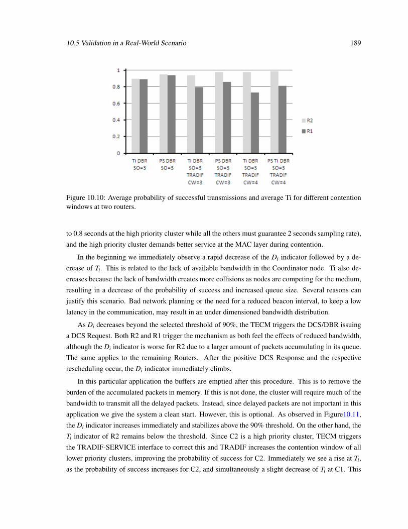
10.5 Validation in a Real-World Scenario 189
Figure 10.10: Average probability of successful transmissions and average Ti for different contentionwindows at two routers.
to 0.8 seconds at the high priority cluster while all the others must guarantee 2 seconds sampling rate),
and the high priority cluster demands better service at the MAC layer during contention.
In the beginning we immediately observe a rapid decrease of the Di indicator followed by a de-
crease of Ti. This is related to the lack of available bandwidth in the Coordinator node. Ti also de-
creases because the lack of bandwidth creates more collisions as nodes are competing for the medium,
resulting in a decrease of the probability of success and increased queue size. Several reasons can
justify this scenario. Bad network planning or the need for a reduced beacon interval, to keep a low
latency in the communication, may result in an under dimensioned bandwidth distribution.
As Di decreases beyond the selected threshold of 90%, the TECM triggers the DCS/DBR issuing
a DCS Request. Both R2 and R1 trigger the mechanism as both feel the effects of reduced bandwidth,
although the Di indicator is worse for R2 due to a larger amount of packets accumulating in its queue.
The same applies to the remaining Routers. After the positive DCS Response and the respective
rescheduling occur, the Di indicator immediately climbs.
In this particular application the buffers are emptied after this procedure. This is to remove the
burden of the accumulated packets in memory. If this is not done, the cluster will require much of the
bandwidth to transmit all the delayed packets. Instead, since delayed packets are not important in this
application we give the system a clean start. However, this is optional. As observed in Figure10.11,
the Di indicator increases immediately and stabilizes above the 90% threshold. On the other hand, the
Ti indicator of R2 remains below the threshold. Since C2 is a high priority cluster, TECM triggers
the TRADIF-SERVICE interface to correct this and TRADIF increases the contention window of all
lower priority clusters, improving the probability of success for C2. Immediately we see a rise at Ti,
as the probability of success increases for C2, and simultaneously a slight decrease of Ti at C1. This

190 Adding Online Cross-layer QoS Control to ZigBee Cluster-based Networks
Figure 10.11: Variation of the Ti and Di indicators as TECM is applied to the network setup.
happens on all other clusters but is not shown in this figure for readability.
As observed Ti stabilizes around 85% for C1. Similar values were found at the other clusters.
After 130 seconds of simulation, the application mode is changed to AM1. The incoming traffic rate
at C0 decreases and as it drops below the specified threshold, the DCS mechanism will trigger a DCS
Request to decrease the service, as the bandwidth is not needed anymore. The schedule returns to the
previous version. In Figure10.11, this is not noticeable in the Di indicator, as it remains always high.
This is because there is no lack of bandwidth. Concerning Ti at R2, a change is visible as C2 loses its
high priority status. R2 issues a RESET using the TRADIF-SERVICE interface and all the clusters
10.5 Validation in a Real-World Scenario 191
reset the TRADIF mechanism, leading to an immediate decrease of Ti in R2 and stabilization around
90%. A slight increase is observed for C1 and all the remaining clusters as the contention window is
reset to its default value (CW = 2), and now share the same priority in contention.
10.5.2.2 TECM Auto-Rate Mode
TECM can also be used in Auto-Rate mode. This mode aims at maximizing the traffic rate of the
selected nodes, using DCS or TRADIF when necessary. This is usually chosen when one does not
care about enforcing a delivery rate but wishes to maximize the use of the available network resources
within predefined performance limits. TECM will periodically tell the application to increase the
traffic rate (the user must implement that in the APL) through the APLTEC-SAP, as long as the Di
performance indicator does not fall beyond a threshold. In that case, TECM will ask the APL to
decrease the traffic rate and trigger a DCS Request in a similar fashion to the Fixed-Rate mode to
increase available bandwidth. Upon re-scheduling, TECM continues the process until no further in-
crease is possible, usually due to a negative DCS Response, at which point the last traffic rate is kept.
Figure 10.12, shows the variation of Di in R2 and N7 (sensing node belonging to C2) for AM2,
as the rate is increased using TECM Auto-Rate mode from 2 packets/second per sensing node up to
15. As the traffic rate climbs beyond 2.4 packets/second, the Di indicator at R2 starts decreasing as its
queue begins to grow. Note that Di in N7 remains the same. As Di goes beyond the threshold, DCS is
triggered and similarly to the previous mode the indicator is reset and packets are purged. A decrease
in the rate to the previous value is carried out as soon as the issue is detected, and Di goes up while
DCS re-scheduling is being carried out, increasing the coordinator node bandwidth by changing its SO
to 3. Importantly, Di at the sensing node is not affected as no more bandwidth is needed. The traffic
rate resumes its increasing rate after the DCS re-schedule and Di remains stable at the two nodes until
a traffic rate of approximately 7 packets/second is reached. At this point, Di at R2 decreases again
beyond the threshold which triggers DCS. Traffic generation is decreased to the previous rate and DCS
increases the Coordinator SO to 4. When a rate of 15 packets/sec is reached, the process is repeated.
However, this time, the Di of node N7 also indicates that more bandwidth is needed to transmit all
the traffic to R2. DCS computes the new scheduling, increasing the coordinator’s SO to 5 and all the
routers SO to 3 (the next SO). At this point, all the BI space is used. The TECM Auto-Rate process
resumes increasing the traffic rate again but Di at node 7 is showing that the available bandwidth is
still not enough to support the specified traffic rate. DCS is triggered, however, as no more space is
available, a negative DCS response is sent. In response, the nodes at depth 2 must maintain a lower
traffic rate. The TECM Auto-Rate process reaches a steady state and remains with those settings until
the user resets TECM.
An interesting observation results from the fact that without TECM, solely relying on the DCS
algorithm would result in a much lower traffic rate due to a non-optimized bandwidth redistribution.

192 Adding Online Cross-layer QoS Control to ZigBee Cluster-based Networks
Figure 10.12: Variation of Di in R2 and N7 (sensing node belonging to C2) for AM2, as the rate isincreased using TECM Auto-Rate mode.
Figure 10.12 depicts the maximum traffic rate that could be achieved if only DCS was used, and
Figure 10.13 shows the resulting schedules.
As presented, solely using the original DCS algorithm would result in the last schedule, as band-
width would be distributed among all the nodes in the streams, increasing each nodes’ SO to 3, quickly
depleting the available space in the BI, even if at that rate, an increase in the coordinator’s bandwidth
would suffice. By using TECM to trigger DCS we added intelligence to the process, only increasing
the bandwidth where needed, allowing for much higher traffic rates as seen in Figure 10.12.
10.6 Conclusions and Future Work
This work presents TECM, a cross-layer QoS management mechanism, providing an automatic and
on-line control of two QoS mechanisms for ZigBee Cluster-tree network based applications. At the
MAC, we improve on the successful transmission probability to achieve traffic differentiation using
TRADIF. At the network level, through DCS we carry out an on-line efficient allocation of the avail-
able bandwidth, reducing the queuing delays and memory requirements per node, which results in the
elimination of bottlenecks in the network infrastructure, and a clear improvement to the end-to-end

10.6 Conclusions and Future Work 193
Figure 10.13: Resulting network schedules as TECM carries out network changes.
latency. Interestingly, we achieve better results than if the mechanism were used separately. This
is a result of the intelligence added by the TECM algorithm, which will increase the bandwidth only
where needed, instead of redistributing it throughout all the clusters. In our evaluation, we were able to
achieve reductions in end-to-end delay in the order of 94% and improvements in the successful trans-
mission probability up to 10% in a real datacenter monitoring application scenario. Latency for any
specific stream can be further reduced if DCS/DCR is used in conjunction with the DBR technique.
We also proposed an extension to the TRADIF mechanism enabling network level communica-
tion, and BPM, a beacon payload management module. We validate and demonstrate our proposal
through simulation in a datacenter monitoring application scenario, which is to be deployed in a new
large-scale datacenter infrastructure, using the WSN as a sensing infrastructure to collect power and
environmental data, with high resolution and timing constraints. The proposal was also implemented
over the TinyOS operating system, and is awaiting deployment at the datacenter facilities, to enable a
fair comparison between simulation and experimental results.
So far only two QoS properties were tackled in our proposal, (the ones that mostly hindered
the prospective application) but we expect to include others in the near future, as the underlying
TECM mechanism design can easily support this. In this line of work, we plan to enable hidden-node
avoidance with this framework in the near future.

194 Adding Online Cross-layer QoS Control to ZigBee Cluster-based Networks

Part IV
Conclusions and Future Work
195


Chapter 11
General Conclusions and Future Work
11.1 Summary of the Results
Modern embedded systems have been enabling a number of smaller, smarter and ubiquitous devices,
creating an eagerness for monitoring and controlling everything, everywhere. This quest for control,
partially fuelled by an increasing desire for energy efficiency and sustainability, is pushing forward the
design of new Wireless Sensor Network (WSN) infrastructures that will support the next generation
of embedded systems - Cyber Physical Systems, which tightly interact with the physical environment
in a ubiquitous and pervasive fashion.
Such cyber-physical systems require a rethinking of the usual computing and networking concepts,
and given that these computing entities closely interact with their environment, they pose new chal-
lenges to WSNs regarding several Quality of Service (QoS) properties, such as in timeliness, scalabil-
ity, energy-efficiency and robustness, among others. However, the current state-of-the-art and state-of-
technology reveals a strong immatureness and a clear lack of solutions (protocols, software/hardware
architectures, technology) in respect to these QoS properties. Therefore, WSNs must be re-designed
to encompass these, if such systems are to become a reality.
In this dissertation, we opted by a hands-on approach to this problem. We clearly understood
that, in order to push forward the technology, it would be important to rely as much as possible in
real-world application scenarios. First, to clearly identify the most prominent challenges, and second,
to validate and demonstrate the mechanisms, algorithms, and add-ons that were going to be proposed
in a realistic and effective way.
Therefore, this thesis relied on the use of standard protocols, particularly the IEEE 802.15.4 and
ZigBee, combined with commercial-off-the-shelf (COTS) technologies as a baseline to enable the
necessary WSN infrastructures. This COTS-based approach besides reducing costs, eased the devel-
opment and enabled a wider diffusion of the proposed mechanisms and implementations.
197

198 General Conclusions and Future Work
Following this strategy, in the second part of this dissertation, we engineered two real-world in-
novative application scenarios: a structural health monitoring system ([SGA+10a], [ARL+11]) and a
datacenter monitoring system ([PTL+15], [TKD+13]).
These application scenarios embody the paradigm of CPS, and enabled us to identify the most
prominent QoS challenges. We also showed how the state-of-the-art lagged behind in effectively
addressing these issues. These QoS aspects were addressed in the third part of this dissertation by
proposing several mechanisms and add-ons to the above mentioned set of protocols, and importantly,
always maintaining backward compatibility with the standards. Also, the proposals were validated
and demonstrated in the two applications scenarios, showing that these network infrastructures have
the potential to be used in real-world cyber-physical applications in the near future, if provided with
the necessary QoS management mechanisms.
These proposals targeted some of the most crucial QoS issues that currently impair these net-
work infrastructures and hinder their adoption namely, timeliness, scalability, robustness and energy-
efficiency.
Timeliness
This thesis addressed the timeliness aspect in several ways, focusing at two layers of the communica-
tions stack: the MAC sub-layer and the NWK layer.
At the NWL layer, the ZigBee cluster-tree topologies are known for a lack of flexibility in adapt-
ing to changes in the traffic or bandwidth requirements at run-time, making these infrastructures not
capable of allocating more bandwidth to a set of nodes sensing a particular phenomena, or reducing
the latency of a data stream. This causes unnecessary delays and longer data transmission times. In
this thesis we proposed a way of dynamically re-scheduling the clusters’ active periods to avoid this.
The DCS mechanism ([SPT13a], [SPT14]) was validated under both application scenarios.
Concerning the MAC sub-layer of the IEEE 802.15.4 protocol, we carried out an experimental
evaluation of a traffic differentiation mechanism, TRADIF [SBAK10], providing the support of differ-
ent traffic classes to the legacy protocol. This mechanism was also extended to support intra-cluster
communications. In addition to timeliness, this mechanism provides and improvement in terms of
energy-efficiency by improving the probability of successful transmissions.
Still at the MAC sub-layer, and to support the real-time traffic demands from both application
scenarios, the IEEE 802.15.4 Guaranteed Time Slot mechanism, missing from most stack implemen-
tations, was also implemented over the TinyOS operating system, providing real-time traffic support
to TinyOS-based applications. The code was submitted to the TinyOS 15.4 working group and it is
now part of the official TinyOS 2 release.
Scalability
Scalability was also addressed in this thesis with the proposal of a mechanism to support inter-cluster
synchronization. SSYNC [TKD+13] enabled nodes within multiple clusters in a ZigBee cluster-tree

11.2 Validation of thesis Statement 199
topology to synchronize to one specific point in time. This is specially important in applications where
nodes in different clusters must carry out some sort of signal acquisition in a synchronized fashion.
This was mandatory, for instance, to scale the structural health monitoring system to multiple clusters,
covering a larger area and extending the system to target larger structures such as tunnels or bridges.
Robustness
In communication networks, robustness is usually related to how well a network setup can adapt to
different circumstances, such as different traffic flows or timeliness requirements, on its own. In many
application scenarios a WSN must be left operating by several days, months or even years without
human interaction. In such scenarios, where the network is quite dynamic, finding the best network
setup (e.g. scheduling, bandwidth allocation), for instance, can become a daunting task if not even an
impossible one, specially for non-expert users.
To address this, in this thesis we proposed an online and cross-layer Traffic Efficiency Control
Module (TECM) [SUT15]. The proposed mechanism works by improving the probability of suc-
cessful transmissions and by minimizing memory requirements and queuing delays, through a careful
tuning of the IEEE 802.15.4 Slotted CSMA-CA parameters (using TRADIF) and an efficient band-
width allocation at the network clusters via DCS. Interestingly, this mechanism was instantiated in the
Datacenter Monitoring application scenario to enable more dynamic application modes.
Energy Efficiency
In this dissertation, this QoS topic is addressed indirectly by the previous proposals. The use of a traffic
differentiation mechanism such as TRADIF enables a higher probability of successful transmissions,
which in turn reduces the amount of energy spent by the high priority nodes at the MAC level, as
discussed in [KANS06].
Similarly, the use of a dynamic cluster scheduling mechanism such as DCS, reduces the amount
of time a data stream takes to be transmitted. The sooner it is transmitted, sooner the node can go into
sleep mode and save energy. Merging both mechanisms under an online and cross-layer module that
can trigger each when needed, clearly improves this aspect of QoS.
11.2 Validation of thesis Statement
In summary, we confirmed the initial hypothesis of this thesis, i.e., the use of IEEE 802.15.4 and
ZigBee set of standard protocols as a baseline, combined with a set of QoS mechanisms can effectively
support the requirements that future cyber-physical systems may impose.
In this dissertation, we proposed a set of mechanisms which effectively solve some of the most
prominent QoS issues on these WSN infrastructures. Importantly, we validated and demonstrated
these proposals over two real-world application scenarios, each presenting an important contribution
to the state-of-the-art in each application area.

200 General Conclusions and Future Work
11.3 Future Directions
In this dissertation, we verified the potential ZigBee tree-based WSN infrastructures had to support
future network embedded systems. However, several QoS challenges had to be addressed first, by
means of new add-ons, in order to fulfil this potential. In this thesis we focused on the most prominent
QoS issues identified in the chosen application scenarios. Nevertheless, there are still may other
aspects that need to be addressed if these systems are to become a reality. Mobility, for instance will
be a key issue in these systems as at least some nodes/agents are likely to be physically or logically
moving relatively to each other. Also, reliability, in particular by ensuring fault-tolerance, is another
fundamental aspect which must be addressed, specially when clustered-based topologies are used, as
a failure in a cluster-head can disable several sibling nodes.
In what follows we elaborate on a few envisaged future research directions trying to locate this
dissertation in the evolving panorama of the Internet of Things.
11.3.1 Towards a QoS Balancing Framework
In our perspective, QoS should be looked at and addressed in a wide and holistic perspective, instan-
tiated in a diverse range of functional and non-functional properties, namely heterogeneity, energy-
sustainability, timeliness, scalability, reliability, mobility, security, cost-effectiveness and invisibil-
ity. This differs from the traditional perspective which mostly associates QoS with bit-rate, network
throughput, message end-to-end delay and bit error rate. Besides, these properties alone do not reflect
the overall quality of the service provided to the user/application.
While, as we have already discussed, in most of these non-functional properties there is still a clear
lack of maturity, an even bigger challenge is to devise network methodologies and tools that are able to
support system designers on balancing these properties in a way that all application requirements are
simultaneously met. This is particularly difficult since most of them are contradictory (i.e. improving
one of them may harm the others). Ideally, the state-of-the-art should reach a point where, similar to a
sound studio mixing table, the network engineer could be provided with a front-end, to balance each
QoS aspect, while hiding the complexity of the QoS mechanisms behind it as much as possible. This
would enable a much easier network setup and deployment, even for the non-expert.
The TECM framework presented in chapter 10 of this dissertation aims at providing an initial but
significant step towards this objective, by proposing an integrated control of two QoS mechanisms
which operate at separate layers of the communications stack, and without expecting significant inter-
action with the network designer, except in setting a few initial parameters. Nevertheless, a more user
friendly front-end to the network designer would be required to ease the configuration process.
The next step would be to extend this framework to encompass other mechanisms such as H-
NAMe, a hidden-node avoidance mechanism, or the i-GAME mechanism which allows the sharing of
a GTS slot by multiple devices. These are just a few examples of already designed mechanisms which

11.3 Future Directions 201
could be adapted to run behind the envisaged front-end control. Similarly, these mechanisms could
be triggered by a decrease of a performance metric, even without the knowledge of the application
or the user, as long as a few "knobs and switches" had been previously set. These switches would
mostly consist of triggering points and other specific settings to each mechanism, always hiding as far
as possible the complexity of each module.
This QoS balancing front-end, would significantly reduce the complexity of setting up these net-
work infrastructures and specially in maintaining them increasing their robustness and accelerating
their adoption.
11.3.2 On the Engineered Application Scenarios
The application scenarios engineered and presented in this dissertation pushed forward on the current
state-of-the-art on each of their respective application areas. Notably, as presented in each respective
chapter (chapters 5 and 6), there was a lack of both commercial and academic solutions to tackle
the proposed application requirements. In this line, it is only logical that we use this momentum to
further develop these prototypes into products, considering that there is a clear and increasing need
for such systems. Civil engineers strive for the possibility to wirelessly monitor, in an accurate way,
the structural health of constructions. Companies try to optimize the energy consumption of their
increasingly power hungry datacenters at all cost.
Clearly, there are a few tune ups to be carried out in these prototypes before they can become a
commercial product. Nevertheless, in this section we would like to focus on the heading we foresee
for their future development.
Concerning the structural health monitoring system, we envisage the design of (distributed) data
processing and classification algorithms (for modal analysis and damage identification). This would
enable an automated and online evaluation of the structural health, which is specially important in
remote areas. Another potentially interesting aspect to include in the future would be actuation. This
could enable systems such as bridge weight-in-motion which so far is only carried out by very spe-
cialized and expensive wired systems.
Concerning the datacenter monitoring prototype, we envisage to support the possibility of creat-
ing models of the room micro-climate conditions to dynamically propose in an automated way, new
dispositions of the servers, and to enable a local actuation of the cooling equipment, avoiding the
over-cooling of the entire room.
11.3.3 Towards a Smarter World
The latest industrial revolution triggered by micro-electronics enabled a multitude of new devices such
as cell phones, GPS receivers, tablets, RFIDs, etc. Computing devices have become cheaper, more
mobile, more distributed, and more pervasive in everyday life, triggering an increasing number of

202 General Conclusions and Future Work
smart objects popping up everywhere around us, which besides the expected computing abilities are
also being fitted with extended sensing and communication capabilities. It is this proliferation of smart
objects that is rapidly leading towards a new communications paradigm, the Internet of Things, where
every object talk to each other, enabling smarter spaces, such as smart-homes, smart-buildings and
eventually smart-cities, improving on energy efficiency and quality of life, and permanently changing
the way individuals perceive the world and interact with it.
This new paradigm calls for a new generation of embedded systems, which is leading towards a
rethinking of the usual computing and networking concepts, to enable a tighter interaction between
embedded computing devices and the physical environment, via sensing and actuating actions - Cy-
ber Physical Systems (CPS). WSN technology quickly stepped up to the challenge by providing a
communication infrastructure to these systems. Interestingly, many communication protocols are still
fighting to become the de facto standard. No one knows which will rise victorious from the arena, or
even if there will be a winner at all. Perhaps, there is no one-size-fits-all applications standard. At the
moment, ZigBee seems to have the right momentum and to offer the necessary flexibility.
Nevertheless, independently of the communication standard, it is mandatory that these WSN en-
abled systems are conceived in a way that the quality of the service (QoS) recognized by their users
(e.g. directly humans or other information systems) is above an acceptable threshold. Unfortunately,
as discussed before, the traditional take on QoS alone does not reflect the overall quality of the service
provided to the user/application. In effect, according to each application/task requirement, which can
be rather diverse, computations and communications must be correct, secure, produced before a given
deadline and with the smallest energy consumption. Moreover, a number of other QoS aspects such
as heterogeneity, maintainability, scalability, robustness, must be taken into consideration to enable
these systems.
The slow pace at which real-world applications are being delivered, contrary to most market stud-
ies forecasts, is proof of the struggle product developers/engineers are facing due to the current state-
of-the-art and state-of-technology. There is a strong immatureness and a clear lack of solutions (pro-
tocols, software/hardware architectures, technology) with respect to these QoS properties. Research-
oriented test-beds exist in a relatively small number and still present quite limited features particularly
in what concerns such QoS issues, which limits research to computer simulation models.
We are aware of these challenges, and in this thesis, we tried to rely as much as possible on real-
world application scenarios to push forward the technology. We contributed on several QoS aspects
but there is still more work to be done. Mobility, fault-tolerance are just another two examples of QoS
aspects in which research is urgently needed. Many application scenarios require mobility, and it is
clear that the inclusion of fault-tolerance mechanisms is fundamental so that systems become reliable.
We hope that the work carried out in this thesis can push forward the current state-of-art and state-
of-technology in the area, contributing to foster the technology, paving the way towards a smarter,
interconnected and better world.

Appendix A
Papers and Materials
A.1 List of papers by the author
Books
S. Tennina, A. Koubaa, R. Daidone, M. Alves, P. Jurcik, R. Severino, M. Tiloca, J. Hauer, N. Pereira,
G. Dini, M. Bouroche and E. Tovar, IEEE 802.15.4 and ZigBee as enabling technologies for low-
power wireless systems with Quality-of-Service constraints, Lecture Notes in Electrical and Computer
Engineering, Springer Berlin Heidelberg, Germany, 2013.
Journals
R. Severino, S. Ullah, E. Tovar, A Cross-layer QoS Management Framework for ZigBee Cluster-Tree
Networks, Springer Telecommunications Systems, 60(4), 2015.
R. Severino, N. Pereira, and E. Tovar, Dynamic cluster scheduling for cluster-tree WSNS, Springer-
Plus Communication Networks, 3(493), 2014.
N. Pereira and S. Tennina and J. Loureiro and R. Severino and B. Saraiva and M. Santos and F.
Pacheco and E. Tovar, A Microscope for the Data Center, To be published in International Journal of
Sensor Networks (IJSNet) Inderscience, 2015.
203

204 Papers and Materials
Conferences and Workshops
R. Severino, N. Pereira, and E. Tovar, Dynamic cluster scheduling for cluster-tree WSNs, IEEE 16th
International Symposium on Object/Component/Service-Oriented Real-Time Distributed Computing,
(ISORC), Germany, 2013.
J. Büsch, R. Daidone, J. Hauer, R. Severino, S. Tennina and M. Tiloca, An Open-Source IEEE
802.15.4 MAC Implementation for TinyOS 2.1, In Poster and Demo Session of the 8th European
Conference on Wireless Sensor Networks (EWSN 2011), pp 15-16, Bonn (Germany), 2011.
R. Severino, M. Batsa, M. Alves, A. Koubâa, A Traffic Differentiation Add-On to the IEEE 802.15.4
Protocol: implementation and experimental validation over a real-time operating system, 13th Eu-
romicro Conference on Digital System Design (DSD’2010), Lille, France, September 2010.
R. Severino, R. Gomes, M. Alves, P. Sousa, E. Tovar, L. Ramos, R. Aguilar, P. Lourenço, A Wire-
less Sensor Network Platform for Structural Health Monitoring: enabling accurate and synchronized
measurements through (COTS + custom)-based design, 5th IFAC International Conference on Man-
agement and Control of Production and Logistics, University of Coimbra, Portugal, September, 2010.
R. Aguilar, L. Ramos, P. Lourenço, R. Severino, R. Gomes, P. G. de Sousa, M. Alves, E. Tovar,
Operational Modal Monitoring of Ancient Structures using Wireless Technology, International Modal
Analysis Conference and Exposition on Structural Dynamics - IMAC-XXVIII, Jacksonville, Florida
USA, 2010.
Technical Reports
R. Severino, N. Pereira, and E. Tovar. Technical report: Dynamic cluster scheduling for cluster-tree
WSNs, CISTER Technical report, CISTER-TR-130205, 2013.
A.2 Materials
Most of the mechanisms implemented in this dissertation in TinyOS are available at the Open-ZB.net
website (http://www.open-zb.net). Remaining code that was developed in the context of the
TinyOS 15.4 Working Group, in particular the IEEE 802.15.4 GTS implementation, is available at the
TinyOS code repository (https://github.com/tinyos/tinyos-main). The implementation
files can be found under /tos/lib/mac/tkn154.

References
[ Wi10] WirelessHART(TM). Industrial communication networks – wireless communica-tion network and commu- nication profiles – wirelesshart(tm). International Elec-trotechnical Commission, (IEC) Std. 62 591, 2010.
[6Lo15] 6LoWPAN Working Group. Ipv6 over low power wpan, 2015. http://datatracker.ietf.org/wg/6lowpan/charter.
[AHS06] Karl Aberer, Manfred Hauswirth, and Ali Salehi. A middleware for fast and flexiblesensor network deployment. In Proceedings of the 32nd international conferenceon Very large data bases, VLDB ’06, pages 1199–1202. VLDB Endowment, 2006.
[APK04] T.F. Abdelzaher, S. Prabh, and R. Kiran. On real-time capacity limits of multihopwireless sensor networks. In Real-Time Systems Symposium, 2004. Proceedings.25th IEEE International, pages 359–370, 2004.
[ARL+10] R. Aguilar, L. Ramos, P.B. Lourenço, R. Severino, R. Gomes, P. Gandra, M. Alves,and E. Tovar. Operational modal monitoring of ancient structures using wirelesstechnology. In Proceedings of the XXVIII International Modal Analysis Confer-ence, IMAC 2010, Jacksonville, Florida, USA, 2010.
[ARL+11] Rafael Aguilar, LuisF. Ramos, PauloB. Lourenço, Ricardo Severino, RicardoGomes, Paulo Gandra, Mario Alves, and Eduardo Tovar. Operational modal mon-itoring of ancient structures using wireless technology. In Tom Proulx, editor, Dy-namics of Civil Structures, Volume 4, Conference Proceedings of the Society forExperimental Mechanics Series, pages 247–256. Springer New York, 2011.
[AS14] ASC-Sensors. Advanced Sensors Calibration - Capacitive Accelerom-eter ASC5631, 2014. http://www.asc-sensors.de/uploads/tx_ascproducts/DB_ASC_5631_Apr2013.qxp_01.pdf.
[Atm15] Atmel. Ieee 803.15.4 stacks, 2015. http://www.atmel.com/products/Wireless/802154/default.aspx.
[BEK+02] Pat Bohrer, Elmootazbellah N. Elnozahy, Tom Keller, Michael Kistler, CharlesLefurgy, Chandler McDowell, and Ram Rajamony. Power aware computing. pages261–289, 2002.
205

206 REFERENCES
[BSR09] N. Boughanmi, Y-Q. Song, and E. Rondeau. Online adaptation of the ieee 802.15.4parameters for wireless networked control systems. In 8th IFAC InternationalConference on Fieldbuses and networks in industrial and embedded systems (FET2009), 2009.
[BW07] R. Burda and C. Wietfeld. A distributed and autonomous beacon scheduling al-gorithm for ieee 802.15.4/zigbee networks. In Mobile Adhoc and Sensor Systems,2007. MASS 2007. IEEE Internatonal Conference on, pages 1–6, 2007.
[CCCP06] Marcello Cinque, Domenico Cotroneo, Giampaolo De Caro, and MassimilianoPelella. Reliability requirements of wireless sensor networks for dynamic struc-tural monitoring. In Proceedings of the International Workshop on Applied Soft-ware Reliability (WASR 2006),, pages 8–13, 2006.
[CKSA07] A. Cunha, A. Koubaa, R. Severino, and M. Alves. Open-zb: an open-source imple-mentation of the ieee 802.15.4/zigbee protocol stack on tinyos. In Mobile Adhocand Sensor Systems, 2007. MASS 2007. IEEE Internatonal Conference on, pages1–12, 2007.
[CMP+09] Matteo Ceriotti, Luca Mottola, Gian Pietro Picco, Amy L. Murphy, Stefan Guna,Michele Corra, Matteo Pozzi, Daniele Zonta, and Paolo Zanon. Monitoring her-itage buildings with wireless sensor networks: The torre aquila deployment. In InProceedings of the 2009 International Conference on Information Processing inSensor Networks (IPSN ’09), pages 277–288. IEEE Computer Society, Washing-ton, DC, USA„ 2009.
[Con15] Contiki. Operating system, online, 2015. http://www.contiki-os.org/.
[CSP+08] Andre Cunha, Ricardo Severino, Nuno Pereira, Anis Koubaa, and Mario Alves.Zigbee over tinyos: implementation and experimental challenges. In 8th Por-tuguese Conference on Automatic Control (CONTROLO’2008), Vila Real, Portu-gal, pages 21–23, 2008.
[CWH09] Hongsik Choi, Ju Wang, and EstherA. Hughes. Scheduling for information gather-ing on sensor network. Wireless Networks, 15(1):127–140, 2009.
[Dai15a] Daintree Networks. 2400e sensor network adaptor, 2015. http://www.daintree.net.
[Dai15b] Daintree Networks. Sensor Network Analyzer (SNA), 2015. http://www.daintree.net.
[DAS13] DASH7 Alliance Mode. An advanced communication system for wide-area lowpower wireless applications and active rfid; dash 7 alliance: Morgan hill, ca, usa,2013.

REFERENCES 207
[DFPD12] Mario Di Francesco, Cristina M. Pinotti, and Sajal K. Das. Interference-freescheduling with bounded delay in cluster-tree wireless sensor networks. In Pro-ceedings of the 15th ACM international conference on Modeling, analysis and sim-ulation of wireless and mobile systems, MSWiM ’12, pages 99–106, New York,NY, USA, 2012. ACM.
[DZXY10] Liu Dan, Qian Zhihong, Zhang Xu, and Li Yue. Research on tree routing improve-ment algorithm in zigbee network. In Multimedia and Information Technology(MMIT), 2010 Second International Conference on, volume 1, pages 89–92, 2010.
[Ecl15] Eclipse. An open development platform, online, 2015. http://www.eclipse.org.
[Eco10] Superstructures. The Economist, 2010. http://www.economist.com/node/17647603.
[EGE02] J. Elson, L. Girod, and D. Estrin. Fine-grained network time synchronization usingreference broadcasts. In In Proceedings of 5th symposium on Operating systemsdesign and implementation. OSDI 2002, Boston, MA, USA, page 147–163, 2002.
[Emb15] EmberZNnet, 2015. http://www.silabs.com/products/wireless/zigbee/Pages/zigbee-software.aspx.
[Eura] European Institute of Innovation and Technology. EIT-ICT-RICH ContikyRepository - IEEE 802.15.4e Implementation. https://github.com/EIT-ICT-RICH/contiki.
[Eurb] European Institute of Innovation and Technology. EIT-ICT-RICHProject - Reliable IP for time synchronized Channel Hopping networks.https://www.eitdigital.eu/eindhoven-innovation-day/eindhoveninnovationday/innovation-activities/rich-eit-digital-initiative/.
[Eurc] European Institute of Innovation and Technology. EIT-ICT-RICH TinyOSRepository - IEEE 802.15.4e Implementation. https://github.com/EIT-ICT-RICH/tinyos-main.
[Evi12] Evidence. Flex embedded platform reference manual. Technical re-port, 2012. http://download.tuxfamily.org/erika/webdownload/manuals_pdf/flex_refman_1_0_2.pdf.
[Evi15] Evidence. Erika real-time operating system, online, 2015. http://erika.sssup.it/.
[FB06] J. Flora and P. Bonnet. Never mind the standard here is the tinyos 802.15.4 stack.technical report 06–10, university of copenhagen, 2006.
[Fle15] Flexipanel. 2.4ghz zigbee ready ieee 802.15.4 rf transceiver, 2015. http://www.flexipanel.com.

208 REFERENCES
[Fre14] Freescale. Zigbee stack, 2014.
[GCNS11] Veselin Ganev, Dave Chodos, Ioanis Nikolaidis, and Eleni Stroulia. The smartcondo: integrating sensor networks and virtual worlds. In Proceedings of the 2ndWorkshop on Software Engineering for Sensor Network Applications, SESENA’11, pages 49–54, New York, NY, USA, 2011. ACM.
[GLVB+03] D. Gay, P. Levis, R. Von Behren, M. Welsh, Brewer E., and D. Culler. The nesclanguage: A holistic approach to networked embedded systems. In Proceedings ofthe Programming Language Design and Implementation., 2003.
[GRS03] S. Ganeriwal, Kumar R., and M. B. Srivastava. Timing-sync protocol for sensornetworks. In Proceedings of 1st international conference on Embedded networkedsensor systems (SenSys’03), Los Angeles, California, USA., pages 138–149, 2003.
[GSGSRHGH12] Antonio-Javier Garcia-Sanchez, Felipe Garcia-Sanchez, David Rodenas-Herraiz,and Joan Garcia-Haro. On the synchronization of ieee 802.15.5 wireless meshsensor networks: Shortcomings and improvements. EURASIP Journal on WirelessCommunications and Networking, 2012(1):198, 2012.
[GXX07] J. Gibson, G.G. Xie, and Yang Xiao. Performance limits of fair-access in sensornetworks with linear and selected grid topologies. In Global TelecommunicationsConference, 2007. GLOBECOM ’07. IEEE, pages 688–693, 2007.
[GY03] G. Gupta and M. Younis. Fault-tolerant clustering of wireless sensor networks. InWireless Communications and Networking, 2003. WCNC 2003. 2003 IEEE, vol-ume 3, pages 1579–1584 vol.3, March 2003.
[GZH08] Shashidhar Gandham, Ying Zhang, and Qingfeng Huang. Distributed time-optimalscheduling for convergecast in wireless sensor networks. Computer Networks,52(3):610 – 629, 2008.
[HASL07] Tibor Horvath, Tarek Abdelzaher, Kevin Skadron, and Xue Liu. Dynamic volt-age scaling in multitier web servers with end-to-end delay control. IEEE Trans.Comput., 56(4):444–458, April 2007.
[Hau09] J.-H. Hauer. Tkn15.4: An ieee 802.15.4 mac—implementation for tinyos 2.tkn technical report tkn-08-003, technical university berlin, telecommunicationnetworks group, department telecommunication networks (tkn), berlin, germany,2009.
[HBT+09] Rob Hoes, Twan Basten, Chen-Khong Tham, Marc Geilen, and Henk Corporaal.Quality-of-service trade-off analysis for wireless sensor networks. PerformanceEvaluation, 66(3–5):191 – 208, 2009. Modeling and Analysis of Wireless Net-works: Selected Papers from {MSWiM} 2007.
[HCB00] Wendi Rabiner Heinzelman, Anantha Chandrakasan, and Hari Balakrishnan.Energy-efficient communication protocol for wireless microsensor networks. In

REFERENCES 209
Proceedings of the 33rd Hawaii International Conference on System Sciences-Volume 8 - Volume 8, HICSS ’00, pages 8020–, Washington, DC, USA, 2000.IEEE Computer Society.
[HCG+06] Taliver Heath, Ana Paula Centeno, Pradeep George, Luiz Ramos, Yogesh Jaluria,and Ricardo Bianchini. Mercury and freon: temperature emulation and manage-ment for server systems. SIGOPS Oper. Syst. Rev., 40(5):106–116, October 2006.
[HDS+11] J.-H. Hauer, R. Daidone, R. Severino, M. Tiloca J. Büsch, and S. Tennina. Posterabstract: An open-source ieee 802.15.4 mac implementation for tinyos 2.1. In inProceedings of 8th European Conference on Wireless Sensor Networks (EWSN),Bonn, Germany, 2011.
[HJ10] Z. Hanzalek and P. Jurcik. Energy efficient scheduling for cluster-tree wireless sen-sor networks with time-bounded data flows: Application to ieee 802.15.4/zigbee.Industrial Informatics, IEEE Transactions on, 6(3):438–450, 2010.
[HKL+06] Tian He, Sudha Krishnamurthy, Liqian Luo, Ting Yan, Lin Gu, Radu Stoleru, GangZhou, Qing Cao, Pascal Vicaire, John A. Stankovic, Tarek F. Abdelzaher, JonathanHui, Bruce Krogh, Tianhe@cs. Umn. Edu S. Krishnamurthy, Liqian Luo, T. Yan,L. Gu, R. Stoleru, G. Zhou, and Qing Cao. Vigilnet: An integrated sensor networksystem for energy-efficient surveillance. ACM Transaction on Sensor Networks,2:1–38, 2006.
[HLhAC05] Tae Hyun, Doo Hwan Lee, Jae hyun Ahn, and Sunghyun Choi. Priority toningstrategy for fast emergency notification in ieee 802.15.4 lr-wpan. In Proceedingsof the 15th Joint Conference on Communications & Information (JCCI), 2005.
[HPH+12] Yu-Kai Huang, Ai-Chun Pang, Pi-Cheng Hsiu, Weihua Zhuang, and Pangfeng Liu.Distributed throughput optimization for zigbee cluster-tree networks. IEEE Trans-actions on Parallel and Distributed Systems, 23(3):513–520, 2012.
[HSC+08] G. Hackmann, F. Sun, N. Castaneda, C. Lu, and S. Dyke. A holistic approachto decentralized structural damage localization using wireless sensor networks. InProceedings of the IEEE Real-Time Systems Symposium (RTSS’08), 2008.
[IDC13] Worldwide internet of things (iot) 2013-2020 forecast: Billions of things, tril-lions of dollars, idc, online, 2013. http://www.idc.com/getdoc.jsp?containerId=243661.
[IEE05] IEEE-802.11 Task Group E. Ieee std 802.11e: Wireless lan medium access control(mac) and physical layer specifications„ 2005.
[IEE07] IEEE-802.11 Task Group. Ieee 802.11-2007: Wireless lan medium access control(mac) and physical layer (phy) specifications, 2007.
[IEE15a] IEEE 802.15 WPAN Task Group 4e (TG4e), 2015. http://www.ieee802.org/15/pub/TG4e.html.

210 REFERENCES
[IEE15b] IEEE 802.15.5. Ieee 802.15 wpan task group 5 (tg5) mesh networking website,2015. http://www.ieee802.org/15/pub/TG5.html.
[IET03] IETF. Rfc 3561 ad hoc on-demand distance vector (aodv) routing, 2003.
[IGKC12] Ozlem Durmaz Incel, Amitabha Ghosh, Bhaskar Krishnamachari, and KrishnakantChintalapudi. Fast data collection in tree-based wireless sensor networks. IEEETransactions on Mobile Computing, 11(1):86–99, 2012.
[ISA09] ISA100.11a. Wireless systems for industrial automation: Process control and re-lated applications, isa100.11a standard, 2009.
[IT06] IEEE-TG15.4. IEEE Standard for Information technology - Telecommunicationsand information exchange between systems - Local and metropolitan area networks- Specific requirements. Part 15.4: Wireless Medium Access Control (MAC) andPhysical Layer (PHY) Specifications for Low-Rate Wireless Personal Area Net-works (WPANs), 2006.
[JK07] Petr Jurcik and Anis Koubâa. The ieee 802.15.4 opnet simulation model: Referenceguide v2.0. Technical report, CISTER Technical Report, 2007.
[JKS+10] Petr Jurcik, Anis Koubâa, Ricardo Severino, Mário Alves, and Eduardo Tovar. Di-mensioning and worst-case analysis of cluster-tree sensor networks. ACM Trans.Sen. Netw., 7(2):14:1–14:47, September 2010.
[JLKK07] Joseph Jeon, Jong Wook Lee, Hyung Seok Kim, and Wook Hyun Kwon. Pecap:Priority-based delay alleviation algorithm for ieee 802.15.4 beacon-enabled net-works. Wirel. Pers. Commun., 43(4):1625–1631, December 2007.
[KANS06] A. Koubaa, M. Alves, B. Nefzi, and Y.-Q. Song. Improving the ieee 802.15.4slotted csma/ca mac for time-critical events in wireless sensor networks. In In Pro-ceedings of the Workshop of Real-Time Networks (RTN 2006), Satellite Workshopto (ECRTS 2006), July 2006.
[KAT06] A Koubaa, M. Alves, and E. Tovar. A comprehensive simulation study of slottedcsma/ca for ieee 802.15.4 wireless sensor networks. In 2006 IEEE InternationalWorkshop on Factory Communication Systems,, pages 183–192, 2006.
[KC06] Tae Hyun Kim and Sunghyun Choi. Priority-based delay mitigation for event-monitoring ieee 802.15.4 lr-wpans. Communications Letters, IEEE, 10(3):213–215, Mar 2006.
[KCA07] A. Koubaa, A. Cunha, and M. Alves. A time division beacon scheduling mecha-nism for ieee 802.15.4/zigbee cluster-tree wireless sensor networks. In Real-TimeSystems, 2007. ECRTS ’07. 19th Euromicro Conference on, pages 125–135, 2007.
[KCAT08] A. Koubâa, A. Cunha, M. Alves, and E. Tovar. Tdbs: A time division beaconscheduling mechanism for zigbee cluster-tree wireless sensor networks. In Real-Time Systems Journal, volume 40, pages 321–354. Springer, December 2008.

REFERENCES 211
[KFS08] V Krishnamurthy, K Fowler, and E Sazonov. The effect of time synchronization ofwireless sensors on the modal analysis of structures. Smart Materials and Struc-tures, 17(5):055018, 2008.
[KKP+07] Taehong Kim, Daeyoung Kim, Noseong Park, Seong-Eun Yoo, and T.S. Lopez.Shortcut tree routing in zigbee networks. In Wireless Pervasive Computing, 2007.ISWPC ’07. 2nd International Symposium on, 2007.
[KKY+07] Eui-Jik Kim, Meejoung Kim, Sung-Kwan Youm, Seokhoon Choi, and Chul-HeeKang. Priority-based service differentiation scheme for {IEEE} 802.15.4 sensornetworks. International Journal of Electronics and Communications, 61(2):69 –81, 2007.
[KM05] J. Fredrik Karlsson and Bahram Moshfegh. Investigation of indoor climate andpower usage in a data center. Energy and Buildings, 37(10):1075 – 1083, 2005.
[Koo11] Jonathan Koomey. Growth in data center electricity use 2005 to 2010. Technicalreport, Analytics Press, Oakland, CA, August 2011. www.analyticspress.com/datacenters.html.
[KPC+07] S. Kim, S. Pakzad, D. Culler, J. Demmel, G. Fenves, S. Glaser, , and M. Turon.Health monitoring of civil infrastructures using wireless sensor networks. In Infor-mation Processing In Sensor Networks, volume 9, pages 254–263. 2007.
[KWHK08] D. Kipnis, A. Willig, J. H. Hauer, and N. Karowski. The angel ieee 802.15.4enhancement layer: Coupling priority queueing and service differentiation. In InProceedings of 14th European Wireless Conference, Prague, pages 1–7, 2008.
[LA12] J. Liu and Terzis A. Sensing data centres for energy efficiency. PhilosophicalTransactions of the Royal Society, (370):136–157, 2012.
[LKL08] Nai-Luen Lai, Chung-Ta King, and Chun-Han Lin. On maximizing the throughputof convergecast in wireless sensor networks. In Song Wu, LaurenceT. Yang, andTonyLi Xu, editors, Advances in Grid and Pervasive Computing, volume 5036 ofLecture Notes in Computer Science, pages 396–408. Springer Berlin Heidelberg,2008.
[LKPP10] E. K. Lee, I. S. Kulkarni, D. Pompili, and M. Parashar. Proactive thermal man-agement in green datacenters. Journal of Supercomputing (Springer), 51(1):1–31,June 2010.
[LL06] Jerome P Lynch and Kenneth J Loh. A summary review of wireless sensors andsensor networks for structural health monitoring. Shock and Vibration Digest,38(2):91–130, 2006.
[LLK+02] J. P. Lynch, K. H. Law, A. S. Kiremidjian, E. Carryer, C. R. Farrar, H. Sohn,D. Allen, B. Nadler, and J. Wait. Laboratory and field validation of a wirelesssensing unit design for structural monitoring. In Proceedings of US-Korea Work-shop on Smart Structural Systems, Pusan, Korea, 2002.

212 REFERENCES
[LLL+09] Chieh-Jan Mike Liang, Jie Liu, Liqian Luo, Andreas Terzis, and Feng Zhao. Rac-net: a high-fidelity data center sensing network. In Proceedings of the 7th ACMConference on Embedded Networked Sensor Systems, SenSys ’09, pages 15–28,New York, NY, USA, 2009. ACM.
[LLYL13] Wei Liang, Shuai Liu, Yutuo Yang, and Shiming Li. Research of adaptive fre-quency hopping technology in wia-pa industrial wireless network. In RuchuanWang and Fu Xiao, editors, Advances in Wireless Sensor Networks, volume 334 ofCommunications in Computer and Information Science, pages 248–262. SpringerBerlin Heidelberg, 2013.
[Loc10] Dave Locke. Mq telemetry transport (mqtt) v3.1 protocol specifica-tion, 2010. http://www.ibm.com/developerworks/webservices/library/ws-mqtt/index.html.
[LWS+08] J. P. Lynch, Y. Wang, R. A. Swartz, K. C. Lu, and C. H. Loh. Implementation of aclosed-loop structural control system using wireless sensor networks. In StructuralControl and Health Monitoring, volume 15, pages 518–539. John Wiley & Sons,Ltd, June 2008.
[Lyn05] Jerome Peter Lynch. Design of a wireless active sensing unit for localized structuralhealth monitoring. In Structural Control and Health Monitoring, volume 12, pages405–423. 2005.
[M.B09] M.Batsa. Supporting Different QoS Levels in Multiple-Cluster Wireless SensorNetworks. PhD thesis, MSc Thesis in Computer Science and Engineering, De-partment of Electronics and Computer Engineering, Indian Institute of Technology(IIT) Roorkee, 2009.
[MdPSP] P. Muthukumaran, R. de Paz, R. Spinar, and D. Pesch. Meshmac: Enabling meshnetworking over ieee 802.15. 4 through distributed beacon scheduling.
[MEM] MEMSIC. Telosb datasheet. www.memsic.com/userfiles/files/Datasheets/WSN/telosb_datasheet.pdf.
[MEM15] MEMSIC. Wsn products, 2015. http://www.memsic.com/wireless-sensor-networks/.
[MGW09] David Meisner, Brian T. Gold, and Thomas F. Wenisch. Powernap: eliminatingserver idle power. In Proceedings of the 14th international conference on Archi-tectural support for programming languages and operating systems, ASPLOS ’09,pages 205–216, New York, NY, USA, 2009. ACM.
[Mic14] Microchip. dspic33f family data sheet, 2014. http://www.microchip.com.
[MJR11] Lucas D. P. Mendes and Joel J.P.C. Rodrigues. Review: A survey on cross-layersolutions for wireless sensor networks. J. Netw. Comput. Appl., 34(2):523–534,March 2011.

REFERENCES 213
[MKSL04] M. Maroti, B. Kusy, G. Simon, and A. Ledeczi. The flooding time synchroniza-tion protocol. In Proceedings of 2nd International Conference On Embedded Net-worked Sensor Systems, Baltimore, MD, USA, pages 39–49, 2004.
[mod02] Modbus over serial line - specification & implementation guide - v1.0, February2002. http://www.modbus.org/docs/Modbus_over_serial_line_V1.pdf.
[Mon12] Gregory Mone. Redesigning the data center. Commun. ACM, 55(10):14–16, Octo-ber 2012.
[NA10] Vinayak Naik and Anish Arora. Exscal: Dealing with scale. In Elena Gaura,Michael Allen, Lewis Girod, James Brusey, and Geoffrey Challen, editors, WirelessSensor Networks, pages 223–244. Springer US, 2010.
[Nan15] NanoRK. Operating system, online, 2015. http://www.nanork.org/projects/nanork/wiki.
[Nat98] National Instruments Corporation, USA. LabView User Manual, Release 8.0.,1998.
[NKDM09] E D N Ndih, N Khaled, and G De Micheli. An analytical model for the contentionaccess period of the slotted ieee 802.15.4 with service differentiation. In ICC 2009,International Conference on Communication, Dresden, 2009.
[NXP15] NXP Semiconductors. Jennet-ip stack, 2015. http://www.nxp.com/products/interface-and-connectivity/wireless-connectivity/2.4-ghz-wireless-solutions/jennet-ip:JENNET-IP.
[NY11] Sukumar Nandi and Aditya Yadav. Cross layer adaptation for qos in wsn. Interna-tional Journal of Computer Networks & Communications, 3(5):287, 2011.
[OGK06] K.-Y. Jang A. Joki J. Paek M. Vieira D. Estrin R. Govindan O. Gnawali, B. Green-stein and E. Kohler. The tenet architecture for tiered sensor networks. In InProceedings of the 4th ACM Conference on Embedded Networked Sensor Systems(Sensys ’06), 2006.
[OPN15] OPNET Technologies Incorporation. Modeler wireless suite, online, 2015. http://www.opnet.com.
[OSE04a] OSEK/VDX. Oil: Osek implementation language, 2004. http://portal.osek-vdx.org/files/pdf/specs/oil25.pdf.
[OSE04b] OSEK/VDX. Standard, 2004. http://portal.osek-vdx.org.
[OZ15] Open-ZB. Online, 2015. http://www.open-zb.net.

214 REFERENCES
[PA07] K. Shashi Prabh and Tarek F. Abdelzaher. On scheduling and real-time capacity ofhexagonal wireless sensor networks. In Proceedings of the 19th Euromicro Confer-ence on Real-Time Systems, ECRTS ’07, pages 136–145, Washington, DC, USA,2007. IEEE Computer Society.
[Pae05] Chintalapudi Krishna Govindan-Ramesh Caffrey John Masri Sami Paek,Jeongyeup. A wireless sensor network for structural monitoring: Performance andexperience. In Proceedings of the Second IEEE Workshop on Embedded NetworkedSensors (EmNetS-II). Sidney, Australia., 2005.
[PCB] PCB-Piezotronics. Model 393B12 Installation and Operating Man-ual. http://www.pcb.com/contentstore/docs/PCB_Corporate/Vibration/products/Manuals/393B12.pdf.
[PCR+09] Paolo Pagano, Mangesh Chitnis, Antonio Romano, Giuseppe Lipari, Ricardo Sev-erino, Mário Alves, Paulo G. Sousa, and Eduardo Tovar. Erika and open-zb: An im-plementation for real-time wireless networking. In Proceedings of the 2009 ACMSymposium on Applied Computing, SAC ’09, pages 1687–1688, New York, NY,USA, 2009. ACM.
[PSK08] Luca Parolini, Bruno Sinopoli, and Bruce H. Krogh. Reducing data center energyconsumption via coordinated cooling and load management. In Proceedings ofthe 2008 conference on Power aware computing and systems, HotPower’08, pages14–14, Berkeley, CA, USA, 2008. USENIX Association.
[PT08] Meng-Shiuan Pan and Yu-Chee Tseng. Quick convergecast in zigbee beacon-enabled tree-based wireless sensor networks. Comput. Commun., 31(5):999–1011,March 2008.
[PTL+15] N. Pereira, S. Tennina, J. Loureiro, R. Severino, B. Saraiva, M. Santos, F. Pacheco,and E. Tovar. A microscope for the data center. International Journal of SensorNetworks (IJSNet), 18(3-4), 2015.
[Ram07] L. Ramos. Damage Identification on Masonry Structures Based on Vibration Sig-natures. PhD thesis, Universidade do Minho, Guimaraes, Portugal., 2007.
[RBR11] A Rowe, M E Berge, and R Rajkumar. Sensor andrew: Large-scale campus-widesensing and actuation. International Business, 55(1):1–14, 2011.
[RC08] Bhaskaran Raman and Kameswari Chebrolu. Censor networks: a critique of "sen-sor networks" from a systems perspective. SIGCOMM Comput. Commun. Rev.,38(3):75–78, July 2008.
[ReT] ReTIsLab. Real-time systems laboratory, pisa, italy. http://retis.sssup.it/.
[RJ07] Jeffrey Rambo and Yogendra Joshi. Modeling of data center airflow and heat trans-fer: State of the art and future trends. Distrib. Parallel Databases, 21(2-3):193–225, June 2007.

REFERENCES 215
[RMS+11] J. A. Rice, K. A. Mechitov, S. H. Sim, B. F. Spencer, and G. A. Agha. Enablingframework for structural health monitoring using smart sensors. Structural Controland Health Monitoring, 18(5):574–587, 2011.
[Row06] Mangharam R. Rajkumar-R. Rowe, A. Rt-link: A time synchronized link protocolfor energy- constrained multi-hop wireless networks. In Proceedings of the 3rdAnnual IEEE Communications Society on Sensor and Ad Hoc Communicationsand Networks, Reston, VA, USA., pages 402–411, 2006.
[SBAK10] R. Severino, M. Batsa, M. Alves, and A. Koubaa. A traffic differentiation add-onto the ieee 802.15.4 protocol: Implementation and experimental validation over areal-time operating system. In Digital System Design: Architectures, Methods andTools (DSD), 2010 13th Euromicro Conference on, pages 501–508, Sept 2010.
[SCI05] R. R. Schmidt, E. E. Cruz, and M. Iyengar. Challenges of data center thermalmanagement. IBM Journal of Research and Development, 49(4.5):709 –723, july2005.
[SCW10] A. J. Stanford-Clark and G. R. Wightwick. The application of publish/subscribemessaging to environmental, monitoring, and control systems. IBM J. Res. Dev.,54(4):396–402, July 2010.
[SEN14] SENODS Project. Sustainable energy-optimized datacenters, 2014. http://www.cister.isep.ipp.pt/projects/senods/.
[SGA+10a] R. Severino, R. Gomes, M. Alves, P. Sousa, E. Tovara, L. Ramos, R. Aguilar, andP. Lourenço. A wireless sensor network platform for structural health monitoring:enabling accurate and synchronized measurements through (cots + custom)-baseddesign. In Procedings of the 5th IFAC International Conference on Managementand Control of Production and Logistics., September 2010.
[SGA+10b] Ricardo Severino, Ricardo Gomes, Mário Alves, P. Sousa, Eduardo Tovar, Luís F.Ramos, Rafael Aguilar, and Paulo B. Lourenço. A wireless sensor network plat-form for structural health monitoring : enabling accurate and synchronized mea-surements through cots+custom-based design. In 5th Conference on Managementand Control of Production Logistics (2010), pages 375–382, 2010.
[SK96] E. Straser and A.S. Kiremidjian. A modular, visual approach to damage monitoringfor civil structures. In Proceedings of the 2nd International Workshop on StructuralControl, Hong Kong, 1996.
[SLA12] G.A. Shah, Weifa Liang, and O.B. Akan. Cross-layer framework for qos sup-port in wireless multimedia sensor networks. Multimedia, IEEE Transactions on,14(5):1442–1455, Oct 2012.
[SLMR05] John A. Stankovic, Insup Lee, Aloysius Mok, and Raj Rajkumar. Opportunities andobligations for physical computing systems. Computer, 38(11):23–31, November2005.

216 REFERENCES
[SMM+09] T. Semprebom, C. Montez, R. Moraes, F. Vasques, and R. Custodio. Distributeddbp: A (m,k)-firm based distributed approach for qos provision in ieee 802.15.4networks. In 14th IEEE International Conference on Emerging Technologies andFactory Automation (ETFA 09), 2009.
[SPT13a] R. Severino, N. Pereira, and E. Tovar. Dynamic cluster scheduling for cluster-treewsns. In Object/Component/Service-Oriented Real-Time Distributed Computing(ISORC), 2013 IEEE 16th International Symposium on, pages 1–8, June 2013.
[SPT13b] R. Severino, N. Pereira, and E. Tovar. Technical report: Dynamic cluster schedulingfor cluster-tree wsns. Technical report, CISTER-TR-130205, 2013.
[SPT14] R. Severino, N. Pereira, and E. Tovar. Dynamic cluster scheduling for cluster-treewsns. SpringerPlus Communication Networks, 3(493), 2014.
[SUT15] Ricardo Severino, Sana Ullah, and Eduardo Tovar. A cross-layer qos managementframework for zigbee cluster-tree networks. Springer Telecommunication Systems,60(4), 2015.
[Tex14] Texas Instruments. Cc2420 transceiver datasheet, 2014.
[Tex15a] Texas Instruments. Chipcon packet sniffer for ieee 802.15.4 cc2420eb, 2015.http://www.ti.com/lsds/ti/wireless_connectivity/overview.page.
[Tex15b] Texas Instruments. Msp430x21x1 microcontroler datasheet, 2015. http://www.ti.com/product/msp430f149.
[Tex15c] Texas Instruments. Smartrf studio, 2015. http://www.ti.com/tool/smartrftm-studio.
[Tex15d] Texas Instruments. Z-stack, 2015. http://www.ti.com/tool/z-stack.
[The07] The Economist. When everything connects. May 2007.
[Tina] TinyOS. 15.4 working group, online. http://www.tinyos.net/scoop/special/working_group_tinyos_154.html.
[Tinb] TinyOS. Main development repository. https://github.com/tinyos/tinyos-main.
[Tinc] TinyOS. Network protocol working group, online. http://tinyos.stanford.edu/tinyos-wiki/index.php/TinyOS_Network_Protocol_Working_Group.
[Tind] TinyOS. Zigbee working group. http://tinyos.stanford.edu/tinyos-wiki/index.php/TinyOS_ZigBee_Working_Group.
[Tin15] TinyOS. Online, 2015. http://www.tinyos.net/.

REFERENCES 217
[TKD+13] Stefano Tennina, Anis Koubaa, Roberta Daidone, Mario Alves, Petr Jurcik, Ri-cardo Severino, Nuno Pereira Marco Tiloca, Jan-Hinrich Hauer, Gianluca Dini,Melanie Bouroche, and Eduardo Tovar. IEEE 802.15.4 and ZigBee as EnablingTechnologies for Low-Power Wireless Systems with Quality-of-Service Constraints,volume Lecture Notes in Electrical Engineering. Springer Berlin Heidelberg, 2013.
[TLB09] E. Toscano and L. Lo Bello. A multichannel approach to avoid beacon collisions inieee 802.15.4 cluster-tree industrial networks. In Emerging Technologies FactoryAutomation, 2009. ETFA 2009. IEEE Conference on, pages 1–9, 2009.
[VLP11] H. Viswanathan, Eun Kyung Lee, and D. Pompili. Self-organizing sensing infras-tructure for autonomic management of green datacenters. Network, IEEE, 25(4):34–40, july-august 2011.
[VODM91] P. Van Overschee and B. De Moor. Subspace algorithms for the stochastic identi-fication problem. In Proceedings of the 30th Conference on Decision and Control,Brighton, England,, 1991.
[VTPVG+14] Xavier Vilajosana, Pere Tuset-Peiro, Francisco Vazquez-Gallego, Jesus Alonso-Zarate, and Luis Alonso. Standardized low-power wireless communication tech-nologies for distributed sensing applications. Sensors, 14(2):2663–2682, 2014.
[WA05] Tewari G. Patel A. Welsh M. Nagpal R. Werner-Allen, G. Firefly-inspired sensornetwork synchronicity with realistic radio effects. In Proceedings of 3rd interna-tional conference on Embedded networked sensor systems (SenSys’05), San Diego,California, USA., page 142–153, 2005.
[WCLL10] Shengquan Wang, Jian-Jia Chen, Jun Liu, and Xue Liu. Power saving design forservers under response time constraint. In Proceedings of the 2010 22nd EuromicroConference on Real-Time Systems, ECRTS ’10, pages 123–132, Washington, DC,USA, 2010. IEEE Computer Society.
[Wei99] Mark Weiser. The computer for the 21st century. SIGMOBILE Mob. Comput.Commun. Rev., 3(3):3–11, July 1999.
[Wel67] Peter D. Welch. The use of fast fourier transform for the estimation of powerspectra: A method based on time averaging over short, modified periodograms.Audio and Electroacoustics, IEEE Transactions on, 15(2):70–73, Jun 1967.
[WF09] Stephen Wilson and Jeremy Frey. The smartlab: Experimental and environmentalcontrol and monitoring of the chemistry laboratory. In Proceedings of the 2009International Symposium on Collaborative Technologies and Systems, CTS ’09,pages 85–90, Washington, DC, USA, 2009. IEEE Computer Society.
[WGJJ09] Matthew J. Whelan, Michael V. Gangone, Kerop D. Janoyan, and Ratneshwar Jha.Real-time wireless vibration monitoring for operational modal analysis of an inte-gral abutment highway bridge. Engineering Structures, 31(10):2224 – 2235, 2009.

218 REFERENCES
[WIA11] WIA-PA. Industrial communication networks – fieldbus specifications – wia-pacommunication network and communication profile, international electrotechnicalcommission (iec) std. 62 061, 2011.
[WiS] Metageek’s wispy. http://www.metageek.net/products/wi-spy/.
[WL10] Otto VanGeet William Lintner, Bill Tschudi. FEMP best practices guide for energy-efficient data center design. 2010. http://www1.eere.energy.gov/femp/pdfs/eedatacenterbestpractices.pdf.
[WTB+12] T. Winter, P. Thubert, A. Brandt, J. Hui, R. Kelsey, P. Levis, K. Pister, R. Struik,J. P. Vasseur, and R. Alexander. Rpl: Ipv6 routing protocol for low-power and lossynetworks, internet engineering task force. RFC 6550, March 2012.
[WTC03] Alec Woo, Terence Tong, and David Culler. Taming the underlying challengesof reliable multihop routing in sensor networks. In Proceedings of the 1st Inter-national Conference on Embedded Networked Sensor Systems, SenSys ’03, pages14–27, New York, NY, USA, 2003. ACM.
[WTS+11] Beat Weiss, Hong Linh Truong, Wolfgang Schott, Thomas Scherer, Clemens Lom-briser, and Pierre Chevillat. Wireless sensor network for continuously monitoringtemperatures in data centers. IBM RZ 3807, 2011.
[WVK+12] Thomas Watteyne, Xavier Vilajosana, Branko Kerkez, Fabien Chraim, KevinWeekly, Qin Wang, Steven Glaser, and Kris Pister. Openwsn: a standards-based low-power wireless development environment. Transactions on EmergingTelecommunications Technologies, 23(5):480–493, 2012.
[XMP] Xmpp standards foundation. http://xmpp.org.
[XRC+04] Ning Xu, Sumit Rangwala, Krishna Kant Chintalapudi, Deepak Ganesan, AlanBroad, Ramesh Govindan, and Deborah Estrin. A wireless sensor network forstructural monitoring. In Proceedings of the 2Nd International Conference on Em-bedded Networked Sensor Systems, SenSys ’04, pages 13–24, New York, NY, USA,2004. ACM.
[XZR+05] Ruibin Xu, Dakai Zhu, Cosmin Rusu, Rami Melhem, and Daniel Mossé. Energy-efficient policies for embedded clusters. In Proceedings of the 2005 ACM SIG-PLAN/SIGBED conference on Languages, compilers, and tools for embedded sys-tems, LCTES ’05, pages 1–10, New York, NY, USA, 2005. ACM.
[YIE11] M. Aykut Yigitel, Ozlem Durmaz Incel, and Cem Ersoy. Qos-aware {MAC} pro-tocols for wireless sensor networks: A survey. Computer Networks, 55(8):1982 –2004, 2011.
[YPT08] Lun-Wu Yeh, Meng-Shiuan Pan, and Yu-Chee Tseng. Two-way beacon schedulingin zigbee tree-based wireless sensor networks. In Sensor Networks, Ubiquitous andTrustworthy Computing, 2008. SUTC 08. IEEE International Conference on, pages130–137, 2008.

REFERENCES 219
[ZA05] ZigBee-Alliance. Zigbee specification. Technical report, June 2005.
[ZG03] Jerry Zhao and Ramesh Govindan. Understanding packet delivery performance indense wireless sensor networks. In Proceedings of the 1st International Conferenceon Embedded Networked Sensor Systems, SenSys ’03, pages 1–13, New York, NY,USA, 2003. ACM.
[ZWBM12] Rongliang Zhou, Zhikui Wang, Cullen E. Bash, and Alan McReynolds. Data centercooling management and analysis – a model based approach. In 28 Annual Semi-conductor Thermal Measurement, Modeling and Management Symposium (SEMI-THERM 2012), San Jose, California, USA, March 2012.
Copyright © 2022 FDOKUMEN