A QUASI-VARIATIONAL INEQUALITY PROBLEM IN SUPERCONDUCTIVITY

A QUASI-VARIATIONAL INEQUALITY PROBLEM

IN SUPERCONDUCTIVITY

JOHN W. BARRETT

Department of Mathematics, Imperial College London,

London SW7 2AZ, [email protected]

LEONID PRIGOZHIN

Department of Solar Energy and Environmental Physics,

Blaustein Institutes for Desert Research,

Ben-Gurion University of the Negev,

Sede Boqer Campus, 84990 [email protected]

Received 19 September 2008

Revised 8 May 2009Communicated by J. Ball

We derive a class of analytical solutions and a dual formulation of a scalar two-space-dimensional

quasi-variational inequality problem in applied superconductivity. We approximate this for-mulation by a fully practical ¯nite element method based on the lowest order Raviart�Thomas

element, which yields approximations to both the primal and dual variables (the magnetic and

electric ¯elds). We prove the subsequence convergence of this approximation, and hence prove

the existence of a solution to both the dual and primal formulations, for strictly star-shapeddomains. The e®ectiveness of the approximation is illustrated by numerical examples with and

without this domain restriction.

Keywords: Superconductivity; Kim model; quasi-variational inequalities; critical-state problems;

mixed methods; ¯nite elements, existence; convergence analysis.

AMS Subject Classi¯cation: 35D05, 35K85, 49J40, 49M29, 65M12, 65M60, 82C27

1. Introduction

1.1. Primal problem

Macroscopically, magnetisation of type-II superconductors can be regarded as an

eddy current problem described by the Faraday and Amp�ere laws

@tb þr � e ¼ 0; r � b ¼ j; ð1:1Þ

Mathematical Models and Methods in Applied SciencesVol. 20, No. 5 (2010) 679�706

#.c World Scienti¯c Publishing Company

DOI: 10.1142/S0218202510004404

679

http://dx.doi.org/10.1142/S0218202510004404

with a nonlinear and, often, multi-valued current-voltage relation characterising the

superconducting material. The magnetic permeability of superconductors is assumed

equal to that of a vacuum and scaled to unity; hence, we will not distinguish between

the magnetic ¯eld and the magnetic °ux density b. Typically, the current-voltage

relation represents the electric ¯eld inside the superconductor, e, as the subgradient

of a convex functional,

e 2 @�ðjÞ; ð1:2Þ

where j is the current density, see Bossavit.9 To model the hysteretic response of

superconductors to variations of the external magnetic ¯elds and transport currents,

it is convenient to formulate these problems as evolutionary variational or quasi-

variational inequalities, see Bossavit9 and Prigozhin.22

Of much interest, for technological applications and in physical experiments, are

the energy loss estimates. Hence, the simultaneous determination of the current

density and the electric ¯eld in a superconductor is often necessary. Unfortunately,

the variational inequality formulations,9,22 which we will call \primal", allow one to

compute only the current density; and determining the electric ¯eld remains di±cult,

e.g. if the relation (1.2) is multi-valued. It has been shown recently, see Barrett and

Prigozhin,6 that a dual variational inequality formulation, based on an equivalent

representation of the current-voltage relation,

j 2 @��ðeÞ; ð1:3Þ

where �� is the convex conjugate of �, can be the basis for an e±cient method for

determining both of the variables in the Bean critical-state model,8 which is the basic

model for the magnetisation of type-II superconductors. Bean's model postulates that

(in an isotropic superconductor) the current density cannot exceed some critical

value, jjðx; tÞj � Jc, the electric ¯eld is parallel to the current density, and is zero

wherever jjðx; tÞj < Jc. In this case, � is the characteristic function of the set of

admissible currents K0; that is,

�ðvÞ ¼ �K 0ðvÞ :¼ 0 if v 2 K0;

þ1 if v 62 K0:

�ð1:4Þ

In this paper we will study a similar dual formulation for the model in which the

critical current density, Jc, depends on the magnetic ¯eld and the inequality becomes

quasi-variational, see Prigozhin.22 Such a modi¯cation of the Bean model, where

Jc ¼ JcðjbjÞ is a monotonically decreasing function of the magnetic ¯eld, has been

proposed by Kim et al.21 to account for the decrease of the magnetic moments in

strong external ¯elds, which is typical of most type-II superconductors. There are also

materials demonstrating a secondary peak in their magnetisation hysteresis loops.

The latter phenomenon, often called \the ¯shtail e®ect", can be described by the

eddy current model with a non-monotonic JcðjbjÞ dependence; see, e.g. Johansen

et al.19 We mention here also the primal variational formulation for a generalised

double critical-state model, see Badía and Lopez2 and Kashima,20 in which � is the

680 J. W. Barrett & L. Prigozhin

characteristic function of the set of admissible currents satisfying jðx; tÞ 2 �ðbðx; tÞÞand �ðbÞ � R3 being a given family of closed convex sets.

Below we consider a simple geometric con¯guration of an in¯nite superconducting

cylinder having a cross section � � R2 and placed into a parallel non-stationary

uniform external magnetic ¯eld beðtÞ. In this case the variational inequality for Bean's

model, and the quasi-variational inequality for Kim's model, are most easily written

in terms of the magnetic ¯eld which has only one non-zero component and can be

regarded as a scalar function.

Let � be a bounded connected domain with a Lipschitz boundary @�; if � is not

simply connected we allow it to have a ¯nite number of \holes" �i; i ¼ 1 ! I; and

set �� ¼ �SðS

i¼1!I��iÞ: In this geometry, the induced magnetic ¯eld wðx; tÞ ¼

bðx; tÞ � beðtÞ is zero on @��, the outer boundary of �, and depends only on time in

each of the holes. We adopt the standard notation for curls in two dimensions:

r� vðxÞ ¼ @x1v2ðxÞ � @x2v1ðxÞ and r � vðxÞ ¼ ½@x2vðxÞ;�@x1vðxÞ�T.To allow for at least some kind of spatial inhomogeneity on � we shall assume

throughout the majority of this paper that

Jcðx; bÞ ¼ kðxÞMðbÞ; ð1:5Þ

where k 2 Cð��Þ, with kðxÞ � k0 > 0 for all x 2 ��, and M : R ! ½M0;M1� � R, with

M0 > 0, are given functions. We do not assume that Jc is monotonically decreasing

with respect to jbj, so we can deal with \the ¯shtail e®ect" mentioned above. In

addition, we do not require M to be continuous for our results on the dual formu-

lation (Q), (1.15a), (1.15b); whereas we do requireM to be continuous for our results

on the primal formulation (P), (1.8).

Using the laws (1.1) and the constitutive relation (1.2), we obtain for any � 2H 1

0ð��Þ that

ð@tb; � � wÞ� � ¼ �ðr � e; � � wÞ�� ¼ �ðe; r � ð� � wÞÞ� �

� �ðr � wÞ � �ðr � �Þ;

where ð�; �Þ�� is the standard inner product on L2ð��Þ: In the Kim and similar models

� ¼ �K 0ðbÞ, the characteristic function of the set of admissible current densities

K 0ðbÞ :¼ fv 2 ½L2ð��Þ�2 : jvðxÞj � Jcðx; bÞ for a:e: x 2 �;

v ¼ 0 a:e: in �i; i ¼ 1 ! Ig: ð1:6Þ

Since, by Amp�ere's law, j ¼ r � b ¼ ½@x2b;�@x1b�T we have that jjj ¼ jrbj ¼ jrwjand so one can replace the set of admissible currents in the variational formulation by

the set of admissible induced magnetic ¯elds. Hence, for any b 2 H 1ð��Þ, we de¯ne

KðbÞ :¼ f� 2 H 10ð��Þ : j r�ðxÞj � Jcðx; bÞ for a:e: x 2 �;

r� ¼ 0 a:e: in �i; i ¼ 1 ! Ig: ð1:7Þ

A Quasi-Variational Inequality Problem in Superconductivity 681

We therefore arrive at a primal variational formulation (quasi-variational

inequality):

(P) Find w 2 L2ð0;T ;Kðwþ beÞÞTH 1ð0;T ;L2ð��ÞÞ such that wð�; 0Þ ¼ w0ð�Þ

and Z T

0

ð@tðwþ beÞ; � � wÞ� � dt � 0 8 � 2 L2ð0;T ;Kðwþ beÞÞ: ð1:8Þ

1.2. Analytical solution of primal problem

For the special case of Bean's model, Mð�Þ M0 > 0 in (1.5), the above inequality is

variational, and its analytical solution for simply connected cross sections is known in

the spatially homogeneous case kð�Þ ¼ k0 > 0, see Barrett and Prigozhin.5 We will

now generalize this solution to the quasi-variational case under the additional

assumption that, initially, the magnetic ¯eld depends only on the distance to the

boundary of the domain �, so that w0ðxÞ ¼ W 0ðdistðx; @�ÞÞ; and then extend it,

under a similar condition, to multiply connected domains �. In applications, for the

geometric con¯guration considered here, the initial magnetic ¯eld is usually uniform,

so this condition is trivially satis¯ed.

Let �� , Jc be given by (1.5) with k 1 and M 2 CðR; ½M0;M1�Þ, and

w0 2 Kðb0Þ, where b0ðxÞ ¼ w0ðxÞ þ beð0Þ. The latter condition implies thatW 0ð0Þ ¼0 and jdsW 0ðsÞj � MðB0ðsÞÞ, where B0ðsÞ ¼ W 0ðsÞ þ beð0Þ. Let us assume ¯rst that

dtbeðtÞ � 0 for all t � 0. Then we de¯ne uðs; tÞ as a solution to the initial value problem

@su ¼ �MðuÞ; uð0; tÞ ¼ beðtÞ:This yields that

uðs; tÞ ¼ F �1ðF ðbeðtÞÞ � sÞ; ð1:9Þwhere F ðsÞ is such that F 0ðsÞ ¼ ½MðsÞ��1 and F ð0Þ ¼ 0: For all t � 0, on noting that

uð0; tÞ ¼ beðtÞ � beð0Þ ¼ B0ð0Þ, we de¯ne the non-negative penetration depth

dðtÞ :¼ supfs : uðr; tÞ � B0ðrÞ 8 r 2 ½0; s�g:We then de¯ne

~bðx; tÞ ¼ Bðdistðx; @�Þ; tÞ; where Bðs; tÞ :¼uðs; tÞ if s 2 ½0; dðtÞ�;B0ðsÞ if s > dðtÞ:

�ð1:10Þ

We claim that ~wðx; tÞ ¼ ~bðx; tÞ � beðtÞ solves the quasi-variational inequality (P).

Obviously, ~wj@� ¼ 0. If dð0Þ ¼ 0 then Bðs; 0Þ B0ðsÞ and ~wðx; 0Þ ¼ w0ðxÞ. Inaddition, since dsB0ðsÞ � �MðB0ðsÞÞ and B0ð0Þ ¼ beð0Þ; we obtain that F ðB0ðsÞÞ �F ðbeð0ÞÞ � s ¼ F ðuðs; 0ÞÞ. Due to the monotonicity of F , this yields that B0ðsÞ �uðs; 0Þ. Hence, if dð0Þ > 0 the equality uðs; 0Þ ¼ B0ðsÞ holds for 0 � s � dð0Þ and so

once again Bðs; 0Þ B0ðsÞ and ~wðx; 0Þ ¼ w0ðxÞ. Next, on setting �T :¼ �� ð0;T Þ,we de¯ne

�þT :¼ fðx; tÞ 2 �T : distðx; @�Þ � dðtÞg:


Then we have a.e. on �þT that r ~wðx; tÞ ¼ @suðs; tÞjs¼distðx;@�Þ r½distðx; @�Þ�, and so

j r ~wðx; tÞj ¼ j@suðs; tÞjs¼distðx;@�Þ ¼ Mð~bðx; tÞÞ. Whereas on ��T :¼ �T n�þ

T , we have

that ~wðx; tÞ ¼ W 0ðdistðx; @�ÞÞ þ beð0Þ � beðtÞ, and so it is easily deduced that

j r ~wðx; tÞj � Mð~bðx; tÞÞ. Therefore ~w 2 Kð~bÞ. As dtbeðtÞ � 0 for all t � 0, it follows

from (1.9) and (1.10) that @tuðs; tÞ � 0, dtdðtÞ � 0, and so @t~b � 0 a.e. on �T . Fur-

thermore, since @t~b ¼ 0 on ��

T , to prove the inequality (1.8) we need to show thatR�þ

T@t~bð� � ~wÞ dx dt � 0 for all � 2 Kð~bÞ. We note that functions from the convex set

Kð~bÞ vanish on @�, and ~w 2 Kð~bÞ decreases with distance from @� on �þT at the

maximal possible rate,Mð~bÞ, for a function inKð~bÞ. Hence we conclude that � � ~w �0 in �þ

T for any � 2 Kð~bÞ, and so the inequality (1.8) is satis¯ed.

If dtbeðtÞ � 0 for all t � 0, an analytical solution can be found in a similar way.

Now uðs; tÞ is a solution to @su ¼ MðuÞ with uð0; tÞ ¼ beðtÞ, and the penetration

depth determined as dðtÞ :¼ supfs : uðr; tÞ � B0ðrÞ 8 r 2 ½0; s�g: Finally, since at

each moment in time these solutions depend only on the distance to the domain

boundary, we can construct an analytical solution to (P) for arbitrary be 2 H 1ð0;T Þby combining the solutions described above.

Solution for a multiply connected domain can be constructed in a similar way by

regarding the hole closures, ��i � ��, as free Dirichlet sets (see Buttazzo and

Stepanov11) and, correspondingly, de¯ning the distance from a point x 2 �� to the

domain boundary as

distDðx; @��Þ

:¼ inf

Z 1

0

kðsðtÞÞjdtsðtÞj dt : s 2 C 0;1ð½0; 1�; ��Þ; sð0Þ ¼ x; sð1Þ 2 @��

;

ð1:11Þ

where

kðxÞ :¼1 if x 2 �;

0 if x 2[Ii¼1

��i:

8><>:

Obviously, distDðx; @��Þ is the same for all points in each hole and, for x 2 �, the

distance is the length of the shortest path to the outer boundary of � assuming the

parts of a path inside holes are not counted. Assuming, for a multiply connected cross

section, that the initial magnetic ¯eld is a function of distDðx; @��Þ and taking into

account that j rdistDðx; @��Þj ¼ 1 a.e. in �, one can now build an analytical solution

to (P) exactly as above but using the distance function (1.11).

1.3. Dual problem

The primal formulation allows one to calculate the magnetic ¯eld and, by Amp�ere's

law, also the current density in a superconductor. Nevertheless, determining the

electric ¯eld remains di±cult and, to solve this problem for the Bean model, several


approaches have been proposed.10,3,6,14 Here we derive a dual (mixed) formulation for

models with critical current density depending on the magnetic ¯eld.

Returning to possibly spatially inhomogeneous Jc de¯ned by (1.5), and recalling

the de¯nition of F in (1.9), F 0ðsÞ ¼ ½MðsÞ��1 and F ð0Þ ¼ 0, we have that the con-

dition j ¼ r � b 2 K0ðbÞ is equivalent to

½MðbÞ��1j ¼ r � F ðbÞ 2 K

:¼ fv 2 ½L2ð��Þ�2 : jvðxÞj � kðxÞ for a:e: x 2 �;

v ¼ 0 a:e: in �i; i ¼ 1 ! Ig:

Note that e 2 @�K 0ðbÞðjÞ means that j 2 K 0ðbÞ and ðe; i � jÞ� � � 0 for any

i 2 K0ðbÞ. The latter is possible if and only if e � ði � jÞ � 0 a.e. in �� for any

i 2 K0ðbÞ. Hence ðe; v � ½MðbÞ��1jÞ� � � 0 for any v 2 K and the current-voltage

relation (1.2), for the choice of � ¼ �K 0ðbÞ, can be rewritten as

e 2 @�K ðr � F ðbÞÞ with its dual form as r � F ðbÞ 2 @��K ðeÞ;

where ��K ðeÞ :¼ sup

v2½L 2ð� �Þ� 2fðe; vÞ� � � �K ðvÞg ¼

Z�

kjej dx: ð1:12Þ

The dual form (1.12) yields for any test ¯eld u that

ðr � F ðbÞ;u � eÞ� � �Z�

kðjuj � jejÞ dx:

We set u ¼ Rv and e ¼ Rq; where R½p1; p2�T :¼ ½p2;�p1�T. Since ðr � F ðbÞ;Rðv � qÞÞ� � ¼ ðr½F ðbÞ�; v � qÞ�� and b� beðtÞ 2 H 1

0ð��Þ, we obtain for all test

¯elds v that Z�

kðjvj � jqjÞ dx þ ðF ðbÞ � F ðbeÞ; r � ðv � qÞÞ�� 0: ð1:13Þ

Similarly, Faraday's law takes the form @tb� r � q ¼ 0.

We introduce the Banach space

V MðDÞ :¼ fv 2 ½Mð �DÞ�2 : r � v 2 L2ðDÞg; ð1:14Þ

whereMð �DÞ is the Banach space of bounded Radon measures; i.e.Mð �DÞ ½Cð �DÞ��,the dual of Cð �DÞ. Our mixed formulation of (P), (1.8), is then:

(Q) Find q 2 L2ð0;T ;V Mð��ÞÞ and b 2 H 1ð0;T ;L2ð��ÞÞ such that bð�; 0Þ ¼ b0ð�Þand Z T

0

ð@tb� r � q; �Þ� � dt ¼ 0 8 � 2 L2ð��T Þ; ð1:15aÞ

Z T

0

Z��

kðjvj � jqjÞ þ ðF ðbÞ � F ðbeÞ; r � ðv � qÞÞ� �

� �dt � 0

8 v 2 L2ð0;T ;V Mð��ÞÞ; ð1:15bÞ

where b0ð�Þ ¼ w0ð�Þ þ beð0Þ and ��T :¼ �� ð0;T Þ.


Clearly, if the pair fq; bg satis¯es (Q), it follows from (1.15b) that rðF ðbÞ �F ðbeÞÞ ¼ 0 in each hole � i and so rb ¼ 0 there as well. In addition, fq þ u; bg is also

a solution of (Q) if suppðuÞ �S

i¼1!I �i and r � u ¼ 0. This corresponds to the well-

known fact that the eddy current problem does not determine the electric ¯eld in non-

conducting media in a unique way. Furthermore, it follows immediately from (1.15a),

(1.15b) that a solution fq; bg of (Q) is such that

q 2 K1ð@tbÞ :¼ fv 2 L2ð0;T ;V Mð�HÞÞ : ðr � v; �Þ� H

T¼ ð@tb; �Þ� H

T8 � 2 L2ð�H

T Þg

and Z T

0

Z��

kjqj ¼ minv2K 1ð@tbÞ

Z T

0

Z��

kjvj: ð1:16Þ

One can exploit this formulation to obtain q if @tb is known. As was shown above, if

k 1 in � and the initial magnetic ¯eld is a function of distDðx; @��Þ, an analytical

solution is known for the solution b of the primal formulation (P); that is,

bðx; tÞ ¼ BðdistDðx; @��Þ; tÞ. One could use this b in (1.16) to recover q. Problems,

similar to (1.16), and their dual formulations have been considered, for simply con-

nected domains, in several works.24,17,18,12,14 We only mention here that the ridge

(cut locus) of the domain plays an important role in the analysis in these works and

that an integral representation of the solution to (1.16) with k 1 has been derived

for � being a polygonal domain18 and for domains with a smooth boundary.12,14

In our analysis of problem (Q) presented below we will also restrict ourselves to

the case when �� and, moreover, assume that the domain � is strictly star-

shaped. The later assumption is to ensure that certain density results hold; see (1.21)

and (1.22a)�(1.22c) below. However, our numerical method applies to the case of a

multiply connected cross section and we will present a numerical example. In ad-

dition, to avoid perturbation of domain errors in our ¯nite element approximation,

we will assume that � is polygonal for ease of exposition.

The outline of this paper is as follows. In the next section we introduce a

regularised version, (Qr), of our mixed formulation, (Q), by smoothing the non-

di®erentiable functionalR�T

jvj by replacing jvjwith 1r jvjr with r > 1.We then consider

the ¯nite element approximation, (Qh;�r Þ, of (Qr) using Raviart�Thomas elements of

the lowest order with vertex sampling on the nonlinear term. We then establish

stability bounds on this approximation, independent of the mesh parameter h, time

step parameter � and the regularisation parameter r. In Sec. 3, under the assumption

(1.5), we prove subsequence convergence of this approximation, as the parameters, h

and � , go to zero and r goes to one, and establish existence of a solution fq; bg to (Q).

Moreover, on further assuming thatM 2 CðR; ½M0;M1�Þ, we show thatw ¼ b� be is a

solution of (P). Finally in Sec. 4, we present some numerical experiments based on the

discretisation (Qh;�r ).

This paper extends the dual formulation in Barrett and Prigozhin6 from vari-

ational to quasi-variational inequalities. We introduce, and prove the convergence of,

a fully practical numerical scheme based on the dual formulation, (Q), which enables


one to approximate simultaneously both the electric and magnetic ¯elds. Hence,

approximating the local rate of energy dissipation, j � e ¼ Jcðx; bÞjej, becomes

straightforward. In proving the existence of a solution to the dual formulation (Q),

we also show the existence of a solution to the primal quasi-variational inequality (P)

involving a gradient constraint. We are not aware of any previous existence results

for (P) in the literature, apart from the analytical solution above which holds for

k 1 and special initial data w0. However, existence results are available in the case

k 1 and M 2 CðR; ½M0;M1�Þ for a modi¯ed problem (Pp) which includes a

p-Laplacian term, and this term plays a crucial role in the analysis.23,1 Finally, we

note that there are existence results20 for a primal quasi-variational 3d formulation of

the double critical-state model where two di®erent constants, Jcjj and Jc?, limit the

magnitudes, respectively, of the parallel and orthogonal (to the magnetic ¯eld)

components of the current density.

1.4. Notation

We end this section with a few remarks about the notation employed in this paper.

Above and throughout we adopt the standard notation for Sobolev spaces on a

bounded domainD with a Lipschitz boundary, denoting the norm ofW ‘;pðDÞ (‘ 2 N,

p 2 ½1;1�) by jj � jj‘;p;D and the semi-norm by j � j‘;p;D. Of course, we have that

j � j0;p;D jj � jj0;p;D. We extend these norms and semi-norms in the natural way to the

corresponding spaces of vector functions. For p ¼ 2, W ‘;2ðDÞ will be denoted by

H ‘ðDÞ with the associated norm and semi-norm written as, respectively, jj � jj‘;D and

j � j‘;D. We setW 1;p0 ðDÞ :¼ f� 2 W 1;pðDÞ : � ¼ 0 on @Dg, andH 1

0ðDÞ W 1;20 ðDÞ. jDj

will denote the measure of D and ð�; �ÞD the standard inner product on L2ðDÞ. When

D �, for ease of notation we write ð�; �Þ for ð�; �Þ�.Let Cð �DÞ denote the space of continuous functions on �D. As one can identify

L1ðDÞ as a closed subspace of the Banach space of bounded Radon measures,

Mð �DÞ ½Cð �DÞ�H; it is convenient to adopt the notationZ�D

j�j jj�jjMð �DÞ :¼ sup

j�j0;1;D�1�2Cð �DÞ

h�; �iCð �DÞ < 1; ð1:17Þ

where h�; �iCð �DÞ denotes the duality pairing on ½Cð �DÞ�H � Cð �DÞ: The condition r �v 2 L2ðDÞ in (1.14) means that there exists u 2 L2ðDÞ such that hv; r�iCð �DÞ ¼�ðu; �ÞD for any � 2 C 1

0ðDÞ.We note that if f�ngn�0 is a bounded sequence in Mð �DÞ, then there exist a

subsequence f�njgnj�0 and a � 2 Mð �DÞ such that as nj ! 1

�nj! � vaguely in Mð �DÞ; i:e: h�nj

� �; �iCð �DÞ ! 0 8 � 2 Cð �DÞ: ð1:18Þ

Moreover, we have that

lim infnj!1

Z�D

j�njj �

Z�D

j�j; ð1:19Þ

see e.g. p. 223 in Folland.16


As well as the Banach space V MðDÞ, recall (1.14), we require for a given s 2 ½1;1�the Banach space

V sðDÞ :¼ fv 2 ½LsðDÞ�2 : r � v 2 L2ðDÞg: ð1:20Þ

We note that V MðDÞ and V sðDÞ for s 2 ½1; 2Þ are not of local type; that is, v 2V MðDÞ ½V sðDÞ� and � 2 C1ð �DÞ does not imply that �v 2 V MðDÞ ½V sðDÞ�, see e.g.p. 22 in Temam.25 Therefore, one has to avoid cuto® functions in proving any

required density results. If � is strictly star-shaped, which we shall assume for the

analysis in this paper, one can show, using the standard techniques of change of

variable and molli¯cation, that

½C1ð��Þ�2 is dense in V sð�Þ if s 2 ð1;1Þ: ð1:21Þ

Moreover, for any v 2 V Mð�Þ, there exist fvjgj�1 2 ½C1ð��Þ�2 such that

vj ! v vaguely in ½Mð��Þ�2 as j ! 1; ð1:22aÞ

r � vj ! r � v weakly in L2ð�Þ as j ! 1; ð1:22bÞ

lim supj!1

Z�

�jvjj dx ¼Z��

�jvj ð1:22cÞ

for any positive � 2 Cð��Þ. We brie°y outline the proofs of (1.21) and (1.22a)�(1.22c). Without loss of generality, one can assume that � is strictly star-shaped with

respect to the origin. Then for v de¯ned on � and � > 1, we have that v�ðxÞ ¼vð��1xÞ is de¯ned on �� :¼ �� . Applying standard Friedrich's molli¯ers J" to v�,

and a diagonal subsequence argument yield, for � ! 1 and " ! 0 as j ! 1, the

desired sequences fvgj�1 demonstrating (1.21) if v 2 V sð�Þ and satisfying (1.22a)�(1.22c) if V Mð�Þ; see e.g. Lemma 2.4 in Barrett and Prigozhin,7 where such tech-

niques are used to prove similar density results.

Finally, throughout C denotes a generic positive constant independent of the

regularisation parameter, r 2 ð1;1Þ, the mesh parameter h and the time step par-

ameter � . Whereas, CðsÞ denotes a positive constant dependent on the parameter s.

2. Numerical Approximation of (Q)

First, we gather together our assumptions on the data.

(A1) Let � � R2 be a strictly star-shaped domain with boundary @�, so that

�� in (P), (1.8), and (Q), (1.15a), (1.15b). Let be 2 H 1ð0;T Þ, k 2 Cð��Þ with

k1 � kðxÞ � k0 > 0 for all x 2 ��, and M : R ! ½M0;M1� � R with M0 > 0. We shall

assume that b0ð�Þ ¼ w0ð�Þ þ beð0Þ with w0 2 Kðb0Þ; i.e. b0ð�Þ � beð0Þ 2 H 10ð�Þ and

j rb0j � kMðb0Þ a.e. in �.

We note that the assumptions (A1) do allow for anMðsÞ that is strictly positive onany bounded interval ofR, but goes to zero as jsj ! 1. This follows since a solution of

(P) is such that w ¼ b� be ¼ 0 on @�� ð0;T Þ and j rwj � k1M1 a.e. in �T . Hence it

follows that jbj � maxt2½0;T � jbeðtÞj þ k1M1 diamð�Þ a.e. on �T . Therefore an MðsÞ


that is strictly positive on any bounded interval, but goes to zero as jsj ! 1 can

always be replaced by

MLðsÞ :¼MðsÞ if jsj � L;

MðLÞ > 0 if jsj � L � k1M1 diamð�Þ þ maxt2½0;T �

jbeðtÞj

(ð2:1Þ

without changing the problem (P).

In order to prove the existence of, and approximate, solutions to (Q), (1.15a),

(1.15b), we introduce F 2 CðRÞ, G 2 C 1ðRÞ such that

F ð0Þ ¼ Gð0Þ ¼ 0; F 0ðsÞ ¼ ½MðsÞ��1 and G 0ðsÞ ¼ F ðsÞ 8 s 2 R: ð2:2Þ

Hence it follows from (A1) that G is strictly convex, i.e.

GðaÞ �GðcÞ < F ðaÞða� cÞ 8 a; c 2 R; a 6¼ c: ð2:3ÞWe note also for later purposes that

ðF ðcÞ � F ðaÞÞc � GðcÞ � F ðaÞc

� c2

2M1

� jajjcjM0

� c2

4M1

� M1a2

M 20

8 a; c 2 R: ð2:4Þ

Next, for any r > 1, we regularise the non-di®erentiable nonlinearity j � j by the

strictly convex functional 1r j � jr. We note for all a, c 2 R2 that

1

r

@jajr@ai

¼ jajr�2ai ) jajr�2a � ða � cÞ � 1

r½jajr � jcjr�; ð2:5aÞ

ðjajr�2a � jcjr�2cÞ � a � r� 1

r½jajr � jcjr�: ð2:5bÞ

In addition, for r 2 ð1; 2� we have that

jjajr�2a � jcjr�2cj � ð1þ 22ð2�rÞÞ 12 ja � cj 8 a; c 2 R

2; ð2:6Þ

see e.g. Lemma 1 in Chow.13

For a given r > 1, we then consider the following regularisation of (Q):

(Qr) Find qr 2 L2ð0;T ;V rð�ÞÞ and br 2 H 1ð0;T ;L2ð�ÞÞ such that brð�; 0Þ ¼b0ð�Þ and Z T

0

ð@tbr � r � qr; �Þ dt ¼ 0 8 � 2 L2ð�T Þ; ð2:7aÞ

Z T

0

½ðkjqrjr�2qr; vÞ þ ðF ðbrÞ � F ðbeÞ; r � vÞ� dt ¼ 0 8 v 2 L2ð0;T ;V rð�ÞÞ: ð2:7bÞ

For ease of exposition, we shall assume that � is a polygonal domain to avoid

perturbation of domain errors in the ¯nite element approximation. We make the

following assumption


(A2) � is polygonal. Let fT hgh>0 be a regular family of partitionings of � into

disjoint open triangles � with h� :¼ diamð�Þ and h :¼ max�2T h h�, so that�� ¼ [�2T h��.

Let @� be the outward unit normal to @�, the boundary of �. We then introduce

the lowest order Raviart�Thomas ¯nite element spaces

V h :¼ fvh 2 ½L1ð�Þ�2 : vhj� ¼ a� þ c�x; a� 2 R2; c� 2 R 8 � 2 T hg � V 1ð�Þ;

ð2:8aÞ

Sh :¼ f�h 2 L1ð�Þ : �hj� ¼ y� 2 R 8� 2 T hg: ð2:8bÞ

Here the constraint V h � V 1ð�Þ yields for all v 2 V h and for all adjacent triangles

�, � 0 2 T h that

vhj� � @� þ vhj� 0 � @� 0 ¼ 0 on @� \ @� 0: ð2:9Þ

Let P h : L1ð�Þ ! Sh be such that

ððI � P hÞz; �hÞ ¼ 0 8 �h 2 Sh: ð2:10Þ

It follows for all s 2 ½1;1�, that if z 2 Lsð�Þ, then

jP hzj0;s;� � jzj0;s;� and limh!0

jðI � P hÞzj0;s;� ¼ 0: ð2:11Þ

In addition, let 0 ¼ t0 < t1 < � � � < tN�1 < tN ¼ T be a partitioning of ½0;T � intopossibly variable time steps �n :¼ tn � tn�1, n ¼ 1 ! N . We set � :¼ maxn¼1!N �nand

bne :¼ beðtnÞ n ¼ 0 ! N: ð2:12Þ

Our fully practical approximation of (Qr) by V h is then:

(Qh;¿r ) For n � 1, ¯nd Qn

r 2 V h and Bnr 2 Sh such that

ðBnr � �n r �Qn

r ; �hÞ ¼ ðBn�1

r ; �hÞ 8 �h 2 Sh; ð2:13aÞ

ðkjQnr jr�2Qn

r ; vhÞh þ ðF ðBn

r Þ � F ðbne Þ; r � vhÞ ¼ 0 8 vh 2 V h; ð2:13bÞ

where B0r ¼ F �1ðP hF ðb0ÞÞ.

Here ðv; zÞh :¼P

�2T hðv; zÞh�, and

ðv; zÞh� :¼ 1

3j�j

X3j¼1

vðP �j Þ � zðP �

j Þ 8 v; z 2 ½Cð��Þ�2; 8 � 2 T h; ð2:14Þ

where fP �j g3

j¼1 are the vertices of �. Hence ðv; zÞh averages the integrand v � z over

each triangle � at its vertices and is exact if v � z is piecewise linear over the parti-

tioning T h. For any r � 1 and for any vh 2 V h, we have from the equivalence of


norms for vh and the convexity of j � jr that

Crðjvhjr; 1Þh� �Z�

jvhjr dx � ðjvhjr; 1Þh� 1

3j�j

X3j¼1

jvhðP �j Þjr 8� 2 T h: ð2:15Þ

It follows from (2.15) that

ðkjvhjr; 1Þh ¼X�2T h

½ð½P hk�jvhjr; 1Þh þ ððI � P hÞkjvhjr; 1Þh�

�X�2T h

ð½P hk� jvhjr; 1Þ � jðI � P hÞkj0;1;�ðjvhjr; 1Þh

� ðkjvhjr; 1Þ � CjðI � P hÞkj0;1;�jvhj r0;r;� 8 vh 2 V h:ð2:16Þ

We note from the de¯nition of B0r , (2.2), (2.11) and (A1) that for all s 2 ½1;1�

jB0r j0;s;� ¼ jF �1ðP hF ðb0ÞÞj0;s;�

� M1jP hF ðb0Þj0;s;�� M1jF ðb0Þj0;s;�

� M1

M0

jb0j0;s;� � C: ð2:17Þ

Theorem 2.1. Let the Assumptions (A1) and (A2) hold. Then for all r > 1, for all

regular partitionings T h of �, and for all �n > 0, there exists a unique solution,

Qnr 2 V h and Bn

r 2 Sh, to the nth step of (Qh;�r ). Moreover, we have that

maxn¼0!N

jBnr j0;� þ max

n¼0!NjF ðBn

r Þj0;� þXNn¼1

�nðk jQnr jr; 1Þh � CðT Þ; ð2:18aÞ

r� 1

rmax

n¼1!NðkjQn

r jr; 1Þh þXNn¼1

�nBn

r � Bn�1r

�n

��2

0;�

þXNn¼1

�nj r �Qnr j

20;� � C:

ð2:18bÞ

Proof. It follows from (2.13a) that

Bnr ¼ Bn�1

r þ �n r �Qnr : ð2:19Þ

On noting this, (2.5a) and (2.3), we see that (2.13b), on noting (2.13a) is the

Euler�Lagrange equation for the strictly convex minimisation problem

minv h2V h

E nr ðvh;Bn�1

r þ �n r � vhÞ; ð2:20aÞ

where

E nr ðvh; �hÞ :¼ �n

rðkjvhjr; 1Þh � �nF ðbne Þðr � vh; 1Þ þ ðGð�hÞ; 1Þ

8 vh 2 V h; 8 �h 2 Sh: ð2:20bÞ


Hence the desired existence and uniqueness results forQnr and Bn

r immediately follow

from this and (2.19).

Choosing �h F ðBnr Þ � F ðbne Þ in (2.13a) and vh Qn

r in (2.13b), and combining

yields that

�nðkjQnr jr; 1Þh þ ðF ðBn

r Þ � F ðbne Þ;Bnr � Bn�1

r Þ ¼ 0: ð2:21Þ

We have from (2.21), (2.3), (2.2), (A1), (2.12) and (2.4) that

ðGðBnr Þ � F ðbne ÞBn

r ; 1Þ þ �nðkjQnr jr; 1Þh

� ðGðBn�1r Þ � F ðbn�1

e ÞBn�1r ; 1Þ � ðF ðbne Þ � F ðbn�1

e Þ;Bn�1r Þ


e ÞBn�1r ; 1Þ þM �1

0 �nbne � bn�1

e

�n

��0;�

jBn�1r j0;�


e ÞBn�1r ; 1Þ þ �n

4M1

jBn�1r j20;� þ M1j�j

M 20

Z tn

tn�1

jdtbej2 dt

� ð1þ �nÞðGðBn�1r Þ � F ðbn�1

e ÞBn�1r ; 1Þ þ M1j�j

M 20

Z tn

tn�1

½jbn�1e j2 þ jdtbej2� dt:

ð2:22ÞIt follows immediately from (2.22) that for n ¼ 1 ! N

ðGðBnr Þ � F ðbne ÞBn

r ; 1Þ � etn ðGðB0rÞ � F ðb0eÞB0

r ; 1Þ þ C

Z tn

0

½jbej2 þ jdtbej2� dt� �

:

ð2:23ÞIn addition, we have from (2.4), (2.10), (A1) and (2.17) that

ðGðB0rÞ � F ðb0eÞB0

r ; 1Þ � ðF ðB0rÞ � F ðb0eÞ;B0

rÞ ¼ ðF ðb0Þ � F ðb0eÞ;B0rÞ

� ½jF ðb0Þj0;1;� þ jF ðb0eÞj�jB0r j0;1;� � C: ð2:24Þ

The ¯rst two bounds in the desired result (2.18a) then follow from (2.23), (2.24),

(2.4), (2.2) and (A1).

Summing (2.22) from n ¼ 1 to N yields, on noting (2.23), (2.24) and (A1), that

ðGðBNr Þ � F ðbNe ÞBN

r ; 1Þ þXNn¼1

�nðkjQnr jr; 1Þh � CðT Þ: ð2:25Þ

Hence the third bound in (2.18a) follows from (2.25), (2.4) and (A1).

Choosing �h ½F ðBnr Þ�F ðBn�1

r Þ��½F ðb ne Þ�F ðb n�1e Þ�

�nin (2.13a), and noting (2.13b) and

(2.5b), yields for n ¼ 2 ! N that

�nBn

r � Bn�1r

�n;½F ðBn

r Þ � F ðBn�1r Þ� � ½F ðbne Þ � F ðbn�1

e Þ��n

� �¼ ðr �Qn

r ;F ðBnr Þ � F ðBn�1

r Þ� � ½F ðbne Þ � F ðbn�1e Þ�Þ

¼ �ðk½jQnr jr�2Qn

r � jQn�1r jr�2Qn�1

r �;Qnr Þh

� � r� 1

rðk½jQn

r jr � jQn�1r jr�; 1Þh ð2:26aÞ


and

�1B1

r � B0r

�1;½F ðB1

rÞ � F ðB0rÞ� � ½F ðb1eÞ � F ðb0eÞ��1

� �¼ ðr �Q 1

r ; ½F ðB1rÞ � F ðB0

rÞ� � ½F ðb1eÞ � F ðb0eÞ�Þ¼ �ðk jQ 1

r jr; 1Þh � ðr �Q 1r ;F ðB0

rÞ � F ðb0eÞÞ: ð2:26bÞ

Next it follows, as W 0r ¼ F �1ðP hF ðw0ÞÞ, r � vh 2 Sh for all vh 2 V h and on noting

(A1) and (2.15), that

�ðr �Q 1r ;F ðB0

rÞ � F ðb0eÞÞ ¼ �ðr �Q 1r ;F ðb0Þ � F ðb0eÞÞ

¼ ðQ 1r ; r½F ðb0Þ�Þ

� ðk; jQ 1r jÞ �

1

rðkjQ 1

r jr; 1Þ þr� 1

rðk; 1Þh

� 1

rðkjQ 1

r jr; 1Þh þ C: ð2:27Þ

Summing (2.26a), including (2.26b) and noting (2.27) yields for n ¼ 1 ! N that

r� 1

rðkjQn

r jr; 1Þh þXn‘¼1

�‘B ‘

r � B ‘�1r

�‘;F ðB ‘

rÞ � F ðB ‘�1r Þ

�‘

� �

� C þXn‘¼1

�‘B ‘

r �B ‘�1r

�‘;F ðb ‘eÞ � F ðb ‘�1

e Þ�‘

� �: ð2:28Þ

The ¯rst two bounds in the desired result (2.18b) then follow from (2.28), (2.2),

(2.12) and (A1), on using a Young's inequality. Finally the third bound in (2.18b)

then follows from the second bound in (2.18b) and (2.19).

3. Convergence of (Qh,¿r ) | Existence Theory for (Q)

As the stability bounds (2.18a), (2.18b) do not control spatial derivatives of

fQnr ;B

nr gN

n¼1, except for fr �Qnr g

Nn¼1; we cannot exploit compactness to get strong

convergence of fBnr gN

n¼1, which we require to pass to the limit in F ðBnr Þ in (Qh;�

r ).

Hence we prove the subsequence convergence of solutions to (Qh;�r ), (2.13a), (2.13b),

to solutions of (Q), (1.15a), (1.15b), as h; � ! 0 and r ! 1 in stages. First, we

introduce the following intermediate problem, a discrete in time approximation of

(Qr) for r > 1:

(Q¿r) For n � 1, ¯nd q n

r 2 V rð�Þ and bnr 2 L2ð�Þ such that

ðbnr � �n r � q nr ; �Þ ¼ ðbn�1

r ; �Þ 8 � 2 L2ð�Þ; ð3:1aÞ

ðkjq nr jr�2q n

r ; vÞ þ ðF ðbnr Þ � F ðbne Þ; r � vÞ ¼ 0 8 v 2 V rð�Þ; ð3:1bÞ

where b0r ¼ b0.

We then show that the unique solution of (Qh;�r ) converges to the unique solution

of (Q �r) as h ! 0, by exploiting the monotonicity result (2.5a) and the monotonicity


of F . In order to achieve this we introduce the generalised interpolation operator

I h : V rð�Þ \ ½W 1;rð�Þ�n ! V h, where r > 1, satisfyingZ@i�

ðv � I hvÞ � @i� ds ¼ 0 i ¼ 1 ! 3; 8� 2 T h; ð3:2Þ

where @� [ 3i¼1@i� and @i� are the corresponding outward unit normals on @i�. It

follows that

ðr � ðv � I hvÞ; �hÞ ¼ 0 8 �h 2 Sh: ð3:3Þ

In addition, we have for all � 2 T h and any s 2 ð1;1� that

jv � I hvj0;s;� � Csh�jvj1;s;� and jI hvj1;s;� � Csjvj1;s;�; ð3:4Þ

e.g. see Lemma 3.1 in Farhloul15 and the proof given there for s � 2 is also valid for

any s 2 ð1;1�. Furthermore, it follows from (2.5a), (2.14) and (3.4) for any r > 1 and

any � 2 T h thatZ�

jI hvjr � ðjI hvjr; 1Þh��

�� Ch�j�j j½I hv�rj1;1;� � Crh�j�j jjvjj r1;1;�

8 v 2 ½W 1;1ð�Þ�2: ð3:5Þ

Hence, similarly to (2.16), it follows from (3.5) and (3.4) that

jðkjI hvjr; 1Þ � ðkjI hvjr; 1Þhj � C½rk1 þ jðI � P hÞkj0;1;�� jjvjj r1;1;�

8 v 2 ½W 1;1ð�Þ�2: ð3:6Þ

Theorem 3.1. Let the Assumptions (A1) and (A2) hold. For all regular

partitionings T h of �, and for all time partitions f�ngNn¼1 and for all r > 1 the unique

solution fQnr ;B

nr gN

n¼1 to (Qh;�r ) is such that as h ! 0

Qnr ! q n

r weakly in ½Lrð�Þ�2; n ¼ 1 ! N; ð3:7aÞ

r �Qnr ! r � q n

r weakly in L2ð�Þ; n ¼ 1 ! N; ð3:7bÞ

Bnr ! bnr strongly in L2ð�Þ; n ¼ 0 ! N; ð3:7cÞ

F ðBnr Þ ! F ðbnr Þ strongly in L2ð�Þ; n ¼ 0 ! N ; ð3:7dÞ

where fq nr ; b

nr gN

n¼1 is the unique solution of (Q �r), (3.1a), (3.1b).

Moreover, we have that

r� 1

rmax

n¼1!Nðkjq n

r jr; 1Þ þXNn¼1

�nj r � q nr j

20;� þ max

n¼0!Njbnr j0;� þ max

n¼0!NjF ðbnr Þj0;�

þXNn¼1

�nbnr � bn�1

r

�n

��2

0;�

þ maxn¼1!N

j rbnr j0;p;� � CðT Þ; ð3:8Þ

where p ¼ rr�1.


Proof. It follows immediately from the bounds (2.18a), (2.18b), (2.15), our

assumptions on k and (2.5a) that there exist fq nr g

Nn¼1 and fbnr gN

n¼0 such that

(3.7a), (3.7b) hold for a subsequence ffQnr ;B

nr gN

n¼1ghj>0 of ffQnr ;B

nr gN

n¼1gh>0, the

bounds on fq nr g

Nn¼1 hold in (3.8) and there exist fbnr ; gn

r gNn¼1 such that as hj ! 0

Bnr ! bnr ; F ðBn

r Þ ! gnr weakly in L2ð�Þ; n ¼ 1 ! N : ð3:9Þ

It follows from (2.11) and (2.2) that as h ! 0

F ðB0rÞ ! F ðb0Þ F ðb0rÞ; B0

r ! b0 b0r strongly in L1ð�Þ: ð3:10Þ

We now show that fq nr ; b

nr gN

n¼1 is a solution of (Q �r). For any � 2 L2ð�Þ, we choose

�h P h� 2 Sh in the hj version of (2.13a). We can now pass to the limit hj ! 0 in

this, and obtain, on noting (3.7b), (3.9) and (2.11), the desired result (3.1a) for

n ¼ 1 ! N .

It follows from (2.13a), (2.13b), (2.5a), the monotonicity of F and (2.16) that for

any vh 2 V h and �h 2 Sh

� �1n ðF ðBn

r Þ � F ðbne Þ;Bn�1r � �h þ �n r � vhÞ

¼ � �1n ðF ðBn

r Þ � F ðbne Þ;Bnr � �h � �n r � ðQn

r � vhÞÞ¼ ðkjQn

r jr�2Qnr ;Q

nr � vhÞh þ � �1

n ðF ðBnr Þ � F ðbne Þ;Bn

r � �hÞ

� r�1ðk½jQnr jr � jvhjr�; 1Þh þ � �1

n ðF ð�hÞ � F ðbne Þ;Bnr � �hÞ

� ðkjvhjr�2vh;Qnr � vhÞ þ r�1½ðkjvhjr; 1Þ � ðkjvhjr; 1Þh�

þ � �1n ðF ð�hÞ � F ðbne Þ;Bn

r � �hÞ � Cr�1jðI � P hÞkj0;1;�jQnr j

r0;r;�: ð3:11Þ

For any v 2 ½C1ð��Þ�2 and � 2 L2ð�Þ, we choose vh I hv and �h P h� in the hj

version of (3.11) with n ¼ ‘, for some integer ‘ 2 ½1;N�. Assuming that B ‘�1r ! b ‘�1

r

strongly in L2ð�Þ as hj ! 0, we can now pass to the limit hj ! 0 in this, and obtain,

on noting (3.1a), (3.7a), (3.9), (2.11), (3.3), (2.6), (3.4) and (3.6) that

� �1‘ ðg ‘

r � F ðb ‘eÞ; b ‘r � � � �‘ r � ðq ‘r � vÞÞ

¼ � �1‘ ðg ‘

r � F ðb ‘eÞ; b ‘�1r � � þ �‘ r � vÞ

� ðkjvjr�2v; q ‘r � vÞ þ � �1

‘ ðF ð�Þ � F ðb ‘eÞ; b ‘r � �Þ8 fv; �g 2 ½C1ð��Þ�2 � L2ð�Þ: ð3:12Þ

As ½C1ð��Þ�2 is dense in V rð�Þ, recall (1.21), and fq ‘r; b

‘rg 2 V rð�Þ � L2ð�Þ, it fol-

lows that (3.12) holds for all fv; �g 2 V rð�Þ � L2ð�Þ. For any ¯xed z 2 V rð�Þ and 2 R>0, choosing v q ‘

r � z and � b ‘r in (3.12) yields that

�½ðkjq ‘r � zjr�2ðq ‘

r � zÞ; zÞ þ ðg ‘r � F ðb ‘eÞ; r � zÞ� � 0: ð3:13Þ

Sending ! 0, and repeating the above for all z 2 V rð�Þ yields that

ðkjq ‘rjr�2q ‘

r; vÞ þ ðg ‘r � F ðb ‘eÞ; r � vÞ ¼ 0 8 v 2 V rð�Þ: ð3:14Þ


For any ¯xed ’ 2 L2ð�Þ and 2 R>0, choosing v q ‘r and � b ‘r � ’ in (3.12)

yields that

�½ðF ðb ‘r � ’Þ � ðg ‘r; ’Þ� � 0: ð3:15Þ

Sending ! 0, and repeating the above for all ’ 2 L2ð�Þ yields that g ‘r ¼ F ðb ‘rÞ,

and hence this and (3.14) yield that (3.1b) holds with n ¼ ‘.

It is a simple matter to show that for a given b ‘�1r 2 L2ð�Þ the solution fq ‘

r; b‘rg is

unique. Hence the whole sequence converges in (3.7a), (3.7b) and weakly in (3.7c),

(3.7d) for n ¼ ‘.

To complete the induction step, we need to show that (3.7c) holds, and hence

(3.7d), for n ¼ ‘. From (3.1a) and (2.13a) with n ¼ ‘ and � �h F ðB ‘rÞ, we have

that

ðb ‘r � B ‘r;F ðb ‘rÞ � F ðB ‘

rÞÞ ¼ ðb ‘r � B ‘r;F ðb ‘rÞÞ � ðb ‘�1

r � B ‘�1r ;F ðB ‘

rÞÞ� �‘ðr � ðq ‘

r �Q ‘rÞ; ½F ðB ‘

rÞ � F ðb ‘eÞ� þ F ðb ‘eÞÞ: ð3:16Þ

Next we note from (3.1b) and (2.13b) with n ¼ ‘ and v q ‘r and vh Q ‘

r that

�ðr � ðq ‘r �Q ‘

rÞ;F ðB ‘rÞ � F ðb ‘eÞÞ

¼ �ðr � q ‘r;F ðB ‘

rÞ � F ðb ‘rÞÞ � ðr � q ‘r;F ðb ‘rÞ � F ðb ‘eÞÞ þ ðr �Q ‘

r;F ðB ‘rÞ � F ðb ‘eÞÞ

¼ �ðr � q ‘r;F ðB ‘

rÞ � F ðb ‘rÞÞ þ ðkjq ‘rjr; 1Þ � ðkjQ ‘

rjr; 1Þh: ð3:17Þ

In addition, we note from (2.16) and (2.5a) that

ðkjq ‘rjr; 1Þ � ðkjQ ‘

rjr; 1Þh

� ðk½jq ‘rjr � jQ ‘

rjr�; 1Þ þ CjðI � P hÞkj0;1;�jQ ‘rj

r0;r;�

� rðkjq ‘rjr�2q ‘

r; q‘r �Q ‘

rÞ þ CjðI � P hÞkj0;1;�jQ ‘rj

r0;r;�: ð3:18Þ

The desired result (3.7c), and hence (3.7d), for n ¼ ‘ follow from combining (3.16)�(3.18) and noting (2.2), (3.7a) for n ¼ ‘, (3.7c) for n ¼ ‘� 1, the weak convergence

versions of (3.7c), (3.7d) for n ¼ ‘ and (2.11).

It follows from (3.10) and the above induction step that the desired results (3.7a)�(3.7d) hold for the stated range of n; and furthermore, fq n

r ; bnr gN

n¼1 is the unique

solution of (Q �r). The ¯rst ¯ve bounds in (3.8) then follow directly from (2.18a),

(2.18b), (3.7a)�(3.7d) and (2.5a).

Finally, we need to prove the sixth bound in (3.8). First, we note from (3.1b), (A1)

and the ¯rst bound in (3.8) that for n ¼ 1 ! N

jðF ðbnr Þ � F ðbne Þ; r � vÞj � k1jq nr j

r�10;r;�jvj0;r;� � r� 1

rjq n

r jr0;r;� þ C

� �jvj0;r;�

� CðT Þjvj0;r;� 8 v 2 V rð�Þ: ð3:19Þ

It follows from (3.19) for any integer n 2 ½1;N �, as C10 ð�Þ is dense in Lrð�Þ, that the

distributional gradient of F ðbnr Þ belongs to the dual of ½Lrð�Þ�2. Hence for n ¼ 1 ! N


we have that r½F ðbnr Þ� 2 ½Lpð�Þ�2 and

jðr½F ðbnr Þ�; vÞj � CðT Þjvj0;r;� 8 v 2 ½Lrð�Þ�2: ð3:20Þ

Choosing vðxÞ ¼ jr½F ðbnr ðxÞÞ�jp�2 r½F ðbnr ðxÞÞ� if j r½F ðbnr ðxÞÞ�j 6¼ 0, and vðxÞ ¼ 0

otherwise, in the above and as F is globally Lipschitz, recall (2.2) and (A1), we obtain

the ¯nal bound in (3.8).

Let

q þr ð�; tÞ :¼ q n

r ð�Þ; bþe ðtÞ :¼ bne ; bþr ð�; tÞ :¼ bnr ð�Þ;

bcrð�; tÞ :¼ðt� tn�1Þ

�nbnr ð�Þ þ

ðtn � tÞ�n

bn�1r ð�Þ t 2 ðtn�1; tn�; n � 1:

ð3:21Þ

It follows from (3.21), (3.8), (2.12) and as be 2 H 1ð0;T Þ that

bþr � bcr ! 0 strongly in L2ð�T Þ; bþe ! be strongly in L1ð0;T Þ

as � ! 0: ð3:22Þ

Adopting the notation (3.21), (Q �r) can be restated as:Z T

0

@bcr@t

� r � q þr ; �

� �dt ¼ 0 8 � 2 L2ð�T Þ; ð3:23aÞ

Z T

0

½ðkjq þr jr�2q þ

r ; vÞ þ ðF ðbþr Þ � F ðbþe Þ; r � vÞ� dt ¼ 0

8 v 2 L2ð0;T ;V rð�ÞÞ: ð3:23bÞ

Theorem 3.2. Let the Assumptions (A1) and (A2) hold. For all time partitions

f�ngNn¼1 and for all r 2 ð1; 2� such that r ! 1 as � ! 0; the unique solution fq þ

r ; bþr g to

(Q �r) is such that there exists a subsequence fq þ

r ; bþr g� j>0 of fq þ

r ; bþr g�>0 and fq; bg 2

L2ð0;T ;V Mð�ÞÞ � ½H 1ð0;T ;L2ð�ÞÞ \ L2ð0;T ;H 1ð�ÞÞ� such that as � j ! 0

q þr ! q vaguely in L2ð0;T ; ½Mð��Þ�2Þ; ð3:24aÞ

r � q þr ! r � q weakly in L2ð�T Þ; ð3:24bÞ

bþr ; bcr ! b weakly in L2ð0;T ;H 1ð�ÞÞ; ð3:24cÞ

@bcr@t

! @b

@tweakly in L2ð�T Þ; ð3:24dÞ

bþr ; bcr ! b strongly in L2ð�T Þ: ð3:24eÞ

Moreover, fq; bg solves (Q), (1.15a), (1.15b) with �� .


Proof. The bound (3.8) yields immediately, on noting that r 2 ð1; 2�, (3.21) and our

assumption (A1) on k, the ¯rst four bounds inZ T

0

j r � q þr j

20;� þ jjbþr jj21;� þ jjbcrjj21;� þ @bcr

@t

��20;�

þ jq þr j

20;r;�

� �dt � CðT Þ: ð3:25Þ

Next we have from (3.1b), with v q nr , (A1) and (3.8) that for n ¼ 1 ! N

k0jq nr j

r0;r;� � ðF ðbne Þ � F ðbnr Þ; r � q n

r Þ � CðT Þjr � q nr j0;�: ð3:26Þ

Therefore the last bound in (3.25) follows immediately from (3.26), (3.21) and the

¯rst bound in (3.25).

The subsequence convergence results (3.24a)�(3.24d) follow immediately from

(3.25) and (3.22). The strong convergence result (3.24e) follows from (3.24c), (3.24d),

a standard compactness result and (3.22). As bcrð�; 0Þ ¼ b0ð�Þ, it follows from the

above that bð�; 0Þ ¼ b0ð�Þ.It follows immediately from passing to the limit � j ! 0 in (3.23a), on noting

(3.24b), (3.24d) and (3.22), that fq; bg satisfy (1.15a) with �� .

Given any z 2 L2ð0;T ; ½C1ð��Þ�2Þ, we choose v q þr � z in (3.23b) to yield, on

noting (2.5a), that

�Z T

0

ðF ðbþr Þ � F ðbþe Þ; r � ðq þr � zÞÞ dt ¼

Z T

0

ðkjq þr jr�2q þ

r ; qþr � zÞ dt

� r�1

Z T

0

ðk½jq þr jr � jzjr�; 1Þ dt: ð3:27Þ

It follows immediately from (3.24b), (3.24e), (2.2) and our assumptions onM that for

any z 2 L2ð0;T ; ½C1ð��Þ�2ÞZ T

0

ðF ðbþr Þ � F ðbþe Þ; r � ðq þr � zÞÞ dt !

Z T

0

ðF ðbÞ � F ðbeÞ; r � ðq � zÞÞ dtas � j ! 0: ð3:28Þ

Next, we note that for any z 2 L2ð0;T ; ½C1ð��Þ�2Þ

r�1

Z T

0

ðkjzjr; 1Þ dt !Z T

0

ðkjzj; 1Þ dt as � j ! 0: ð3:29Þ

Finally, it follows from (3.24a), and similarly to (1.19), that

lim inf� j!0

r�1

Z T

0

ðkjq þr jr; 1Þ dt � lim inf

� j!0

Z T

0

ðkjq þr j; 1Þ dt �

Z T

0

Z��

kjqjr� �

dt: ð3:30Þ

Combining Eqs. (3.27)�(3.30), it follows that fq; bg satisfy (1.15b) for any

v 2 L2ð0;T ; ½C1ð��Þ�2Þ. The desired result, fq; bg satis¯es (1.15b) with �� for

any v 2 L2ð0;T ;V Mð�ÞÞ, and hence fq; bg solves (Q) with �� , then follows from

the density results (1.22a)�(1.22c).

Theorem 3.3. Let the assumptions of Theorem 3.2 hold. In addition, let M 2 CðR;½M0;M1�Þ. We then have that any solution fq; bg of (Q) with �� is such that


w ¼ b� be 2 L2ð0;T ;Kðwþ beÞÞ \H 1ð0;T ;L2ð�ÞÞ and wð�; 0Þ ¼ w0ð0Þ. In addition,

we have that Z T

0

Z��

kMðwþ beÞjqj þ ðw; r � qÞ� �

dt ¼ 0: ð3:31Þ

Moreover, w solves the quasi-variational inequality (P), (1.8), with �� .

Proof. We adapt the proof of Theorem 3.2 in Barrett and Prigozhin.6 Any solution

fq; bg of (Q) yields that w ¼ b� be 2 H 1ð0;T ;L2ð�ÞÞ and wð�; 0Þ ¼ w0ð�Þ. Let

ZðvÞ :¼Z T

0

Z��

kjvj þ ðF ðbÞ � F ðbeÞ; r � vÞ� �

dt: ð3:32Þ

It follows from (1.15b) with �� and (3.32) that

ZðqÞ ¼ Z :¼ minv2L 2ð0;T ;V Mð�ÞÞ

ZðvÞ � Zð0Þ ¼ 0: ð3:33Þ

If Z < 0 then, for any minimizing sequence fvjg, we obtain that Zð2vjÞ ! 2Z < Z,

which is a contradiction. Hence Z ¼ 0, and so we have that ZðvÞ � 0 ¼ ZðqÞ for anyv 2 L2ð0;T ;V Mð�ÞÞ. Since this is true also for �v, we obtain thatZ T

0

ðF ðbeÞ � F ðbÞ; r � vÞ dt��

�� Z T

0

Z��

kjvj� �

dt

8 v 2 L2ð0;T ;V Mð�ÞÞ ð3:34aÞ

and Z T

0

ðF ðbeÞ � F ðbÞ; r � qÞ dt ¼Z T

0

Z��

kjqj� �

dt: ð3:34bÞ

It follows from (3.34a), as C10 ð0;T ; ½C1

0 ð�Þ�2Þ is dense in L1ð0;T ; ½L1ð�Þ�2Þ and

k 2 Cð��Þ, that the distributional gradient of F ðbÞ belongs to the dual of

L1ð0;T ; ½L1ð�Þ�2Þ. Hence, as kðxÞ � k0 > 0 for all x 2 ��, we have that r½F ðbÞ� 2L1ð0;T ; ½L1ð�Þ�2Þ andZ T

0

ðk�1 r½F ðbÞ�; vÞ dt��

�� jjvjjL1ð�T Þ 8 v 2 L1ð0;T ; ½L1ð�Þ�2Þ: ð3:35Þ

For any p 2 ½1;1Þ, choosing vðx; tÞ ¼ j½kðxÞ��1 r½F ðbðx; tÞÞ�jp�2½kðxÞ��1 r½F ðbðx;tÞÞ� if j r½F ðbðx; tÞÞ�j 6¼ 0, and vðx; tÞ ¼ 0 otherwise, in the above, and noting the

continuity of the p norm for p 2 ½1;1�, we obtain that

jjk�1 r½F ðbÞ�jjL1ð�T Þ � 1: ð3:36Þ

It follows from (3.34a) and (3.36) thatZ T

0

Z@�

½F ðbÞ � F ðbeÞ�v � n ds

� �dt

�� 2k1jjvjjL1ð�T Þ 8 v 2 L2ð0;T ;V 2ð�ÞÞ;

ð3:37Þ


where n is the outward unit normal to @�. Without loss of generality, we can assume

that � is strictly star-shaped with respect to the origin and so ½x � nðxÞ� � n0 > 0 for

a.e. x 2 @�. Choosing v ¼ �j½F ðbÞ � F ðbeÞ�x in (3.37), where �j 2 H 1ð�Þ is such

that �j ¼ 1 on @� and jj�jjjL1ð�Þ ! 0 as j ! 1, yields that F ðbÞ ¼ F ðbeÞ a.e. on

@�� ð0;T Þ and hence b ¼ be a.e. on @�� ð0;T Þ. For example, one can choose �j in

the following way. For integers j � 1, let �j 2 H 1ð�Þ be the extension by zero to

�j :¼ j�1j � of the unique solution of Laplace's equation in �n�j satisfying the

Dirichlet boundary conditions �j ¼ 1 on @� and �j ¼ 0 on @�j. The weak maximum

principle yields that �jðxÞ 2 ½0; 1� for a.e. x 2 �, and so jj�jjjL1ð�Þ ! 0 as j ! 1.

Combining b ¼ be a.e. on @�� ð0;T Þ with (3.36) yields, on recalling (2.2), that

w ¼ b� be 2 L2ð0;T ;Kðwþ beÞÞ with �� .

Let fqjgj�1 2 L2ð0;T ; ½C1ð��Þ�2Þ satisfy (1.22a)�(1.22c), with v q, for a.a.

t 2 ð0;T Þ. It follows as w 2 L2ð0;T ;Kðwþ beÞÞ that

0 �Z�T

½kMðbÞjqjj þ wr � qj� dx dt

¼Z�T

½kMðbÞjqjj � rw � qj� dx dt

¼Z�T

MðbÞ½kjqjj � r½F ðbÞ� � qj� dx dt

� M1

Z�T

½kjqjj � r½F ðbÞ� � qj� dx dt

¼ M1

Z�T

½kjqjj þ ½F ðbÞ � F ðbeÞ�r � qj� dx dt: ð3:38Þ

Passing to the limit j ! 1 in (3.38), on noting (1.22a)�(1.22c), (3.34b) and that

M 2 CðR; ½M0;M1�Þ, yields the desired result (3.31). Similarly, we have for any � 2Kðwþ beÞ thatZ

�T

�r � qj dx dt ¼ �Z�T

r� � qj dx dt � �Z�T

kMðwþ beÞjqjj dx dt; ð3:39Þ

and hence that Z T

0

ð�; r � qÞ dt � �Z T

0

Z��

kMðwþ beÞjqj� �

dt: ð3:40Þ

Choosing � � � w in (1.15a) with �� and � 2 L2ð0;T ;Kðwþ beÞÞ, and

noting (3.31) and (3.40), yields that w solves the primal variational inequality

(P), (1.8).

4. Numerical Experiments

To compute the unique solution fQnr ;B

nr g of our approximation ðQh;�

r Þ at the nth

time step we substitute (2.19) into (2.13b). This yields a nonlinear problem for


Q :¼ Qnr 2 V h:

ðkjQjr�2Q; vhÞh þ ðF ðBn�1r þ �n r �QÞ � F ðbne Þ; r � vhÞ ¼ 0 8 vh 2 V h; ð4:1Þ

which we solved iteratively. At the ðjþ 1Þth iteration, we ¯rst solve the following

linear problem for Qjþ 12 2 V h:

ðF ðBn�1r þ �n r �QjÞ; r � vhÞþ �nð½MðBn�1

r þ �n r �QjÞ��1 r � ðQjþ 12 �QjÞ � F ðbne Þ; r � vhÞ

þ ðk½jQjjr�2Qj þ jQjj r�2" ðQjþ 1

2 �QjÞ�; vhÞh ¼ 0 8 vh 2 V h; ð4:2Þ

where jvj" :¼ ðjvj2 þ "2Þ 12 with " 1, and we have recalled that F 0ðsÞ ¼ ½MðsÞ��1.

Clearly, the linear system (4.2) is well-posed. Finally we set Qjþ1 ¼ �Qjþ 12 þ

ð1� �ÞQj, where � � 1 is an over-relaxation parameter. In all of our examples below,

we choose r ¼ 1þ 10�7, " ¼ 10�9 and � ¼ 1:2.

Let E h be the set of edges of T h, and �eðxÞ be the vector basis function associated

with the edge e 2 E h in the Raviart�Thomas ¯nite element space V h, see

e.g. Bahriawati and Carstensen4 for details. Then any vh 2 V h can be represented asPe2E h vh

e�e, and we de¯ne jjvhjjE h :¼P

e2E h jvhe jjej. Our stopping criterion for the

above iterative scheme was

jjQjþ1 �QjjjE h

jjQjþ1jjE h

� "NL;

where "NL is a given tolerance. We set "NL ¼ 2 � 10�4 throughout the examples below.

When this stopping criterion was satis¯ed, we set Qnr ¼ Qjþ1 and computed the

magnetic ¯eld Bnr using (2.19). We used the MATLAB PDE Toolbox for the domain

triangulation, and curved domains were approximated by polygons. The ¯nite

element meshes in our examples below contained about 7000 triangles.

As in Barrett and Prigozhin,6 the parameters in the numerical simulations were

chosen on assuming that the dimensionless variables ðx; t; . . .Þ were obtained from the

original variables ðx 0; t 0; . . .Þ as follows:

x ¼ x 0

L; t ¼ t 0

t0; j ¼

j 0

j0; b ¼ b 0

Lj0; e ¼ e 0t0

L2j0;

where L is the characteristic cross section size (the maximal horizontal extension in

the plots below), j0 is the value of the critical current density Jc for a zero magnetic

¯eld, and the superconductors were homogeneous with kðxÞ 1. In the examples

below we assumed that jdtb 0ej is a constant, which was scaled to unity by choosing the

time scale t0 appropriately.

In our numerical simulations, the time step was uniform with � ¼ 0:005. Initially,

the magnetic ¯eld was zero, i.e. w0 beð0Þ ¼ 0, and we assumed a growing external

¯eld, beðtÞ ¼ t; except for the last example on hysteresis.

As our ¯rst example we compare, see Fig. 1, for a rectangular cross section

�, the Bean model (Jc ¼ 1 in dimensionless variables) with the Kim model,


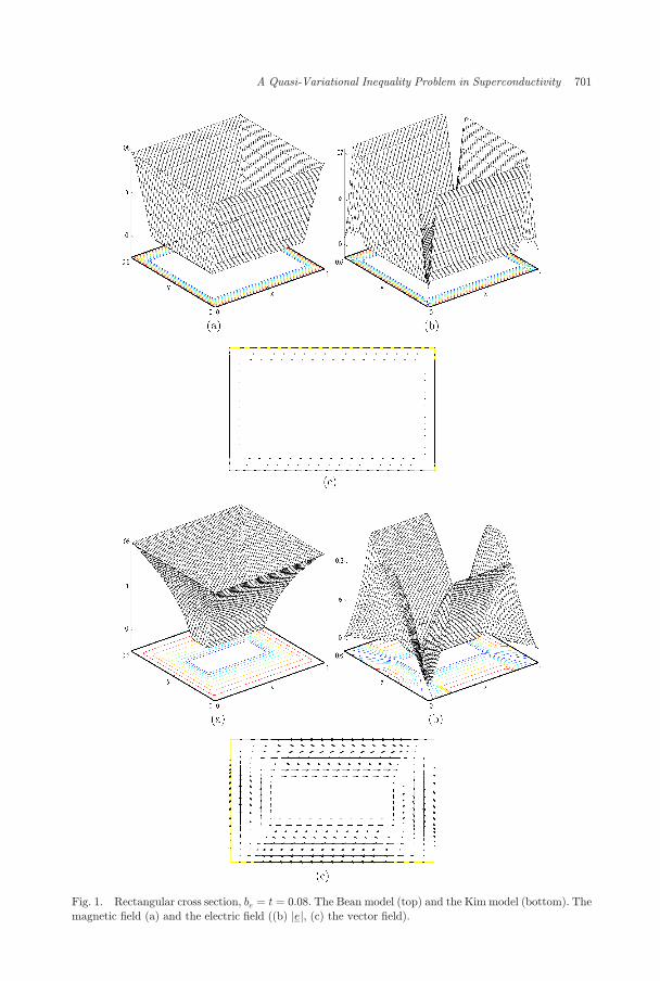
Fig. 1. Rectangular cross section, be ¼ t ¼ 0:08. The Bean model (top) and the Kim model (bottom). The

magnetic ¯eld (a) and the electric ¯eld ((b) jej, (c) the vector ¯eld).


JcðsÞ ¼ ð1þ jsja Þ�1; here and below we set a ¼ 0:02 for this model. Since the critical

current density in the Kim model decreases with the growth of magnetic ¯eld, the

shielding eddy current is weaker and magnetic ¯eld penetrates further inside the

superconductor; this ¯eld, b ¼ ~b, is given by (1.10). To estimate the accuracy of our

numerical solution Bnr we compared it with ~B

n 2 Sh, where ~Bnj� ¼ ~bðx�; tnÞ and x�

is the centroid of � for all � 2 T h. We obtained that

jj ~Bn � Bnr jj0;1;�

jj ~Bn � beðtnÞjj0;1;�< 0:002:

The electric ¯eld found using Kim's model is stronger, but qualitatively similar to

that in the Bean model.10 It has the same zig-zag shape, is zero in the zero-magnetic-

¯eld core, it is parallel to level contours of the magnetic ¯eld, and vanishes along the

discontinuity lines of the current density. Near concave corners of � the electric ¯eld

becomes singular, see Fig. 2 where � is a circle with a section removed.

(a) (b)

(c)

Fig. 2. Circular cross section with a section removed, be ¼ t ¼ 0:07, and the Kim model. The magnetic

¯eld (a) and the electric ¯eld ((b) jej, (c) the vector ¯eld).


Although our analysis in Secs. 2 and 3 holds only for continuous kðxÞ � k0 > 0,

our numerical method (Qh;�r ) extends to piecewise constant k, where the dis-

continuities are aligned with the mesh. Therefore one can simulate numerically the

magnetisation of a superconductor with a multiply connected cross section, see Fig. 3,

by ¯lling the hole and setting k ¼ k0 1 there. For this example, we chose k0 ¼ 10�6

and so the eddy current in the hole is negligible; as in the other examples, k 1 in the

superconductor. Similarly to the Bean model6 when the penetration zone reaches the

hole boundary, the magnetic ¯eld begins to penetrate the hole via an in¯nitesimally

thin channel and the electric ¯eld becomes singular. This singularity is evident in

Fig. 3, although the channel is slightly smeared by the relatively coarse mesh. For a

cross section with only one hole, �1, we have that distDðx; @��Þ ¼ minfdistðx; @��Þ;distðx; @�1Þ þ distð@�1; @�

�Þg: Calculating this distance is not di±cult and we can

substitute it into the derived analytical solution for the magnetic ¯eld, see Sec. 1.2,

for multiply connected cross sections. The relative error in the L1 norm, estimated as

(a)

(b)

Fig. 3. Cross section with a hole, be ¼ t ¼ 0:09, and the Kim model. The magnetic ¯eld (a) and the

electric ¯eld (level contours of jej and vector ¯eld, (b)).


in the ¯rst example, was 0.011 for a mesh with about 7000 elements and 0.007 for a

re¯ned mesh with about 15,000 elements (the same time step, � ¼ 0:005, was used in

both cases).

The di®erence between various critical state models is best exhibited by the

corresponding magnetisation loops, showing the behaviour of the magnetic

momentum of a superconductor when the external ¯eld changes cyclically. For the

longitudinal con¯guration considered in this paper, the magnetic moment of a

superconductor per unit of length is m ¼R�ðbðx; tÞ � beðtÞÞ dx. The hysteresis loops

in Fig. 4 were computed for the superconductor with a rectangular cross section as in

the ¯rst example for three di®erent models: the Bean model, the Kim model, and

a model with a secondary peak in the Jcð�Þ dependence. In the latter case the

critical current density was taken similar to that in Johansen et al.19; that is,

JcðsÞ ¼ ð1þ jsja jÞ�1 þ c1ððjsja � c2Þ2 þ c23Þ�1, in dimensionless variables, with a ¼

0:02 as in the Kim model, c1 ¼ 1, c2 ¼ 8 and c3 ¼ 1.

-0.4 0 0.4

-0.05

0

0.05

m

he

(a)

-0.4 0 0.4

-0.03

0

0.03

he

m

(b)

-1 -0.5 0 0.5

-0.05

0

0.05

he

m

(c)

Fig. 4. Hysteresis loops (dimensionless variables): Bean's model (a), Kim's model (b), and the model with

a secondary peak in JcðbÞ (c).


In conclusion, we note that although quasi-variational inequalities, arising in

critical-state problems with critical current density depending on the magnetic ¯eld,

are much more di±cult mathematical problems than the variational inequalities

arising in Bean's model, their numerical solution based on the dual formulation

presented in this work is practically as e±cient as the solution of the Bean model

problems in Barrett and Prigozhin.6

Acknowledgement

We acknowledge support of the Sixth EU Framework Programme �� Transnational

Access implemented as Speci¯c Support Action (Dryland Research SSA).

References

1. A. Azevedo and L. Santos, Convergence of convex sets with gradient constraint, J.Convex Anal. 11 (2004) 285�301.

2. A. Badía and C. López, The critical state in type II superconductors with cross-°owe®ects, J. Low Temp. Phys. 130 (2003) 129�153.

3. A. Badía-Majós and C. López, Electric ¯eld in hard superconductors with arbitrary crosssection and general critical current law, J. Appl. Phys. 95 (2004) 8035�8040.

4. C. Bahriawati and C. Carstensen, Three Matlab implementations of the lowest-orderRaviart�Thomas MFEM with a posteriori error control, Comput. Meth. Appl. Math.5 (2005) 333�361.

5. J. W. Barrett and L. Prigozhin, Bean's critical-state model as the p ! 1 limit of anevolutionary p-Laplacian, Nonlinear Anal. 42 (2000) 977�993.

6. J. W. Barrett and L. Prigozhin, Dual formulations in critical state problems, Interfacesand Free Boundaries 8 (2006) 347�368.

7. J. W. Barrett and L. Prigozhin, A mixed formulation of the Monge�Kantorovichequations, M 2AN 41 (2007) 1041�1060.

8. C. P. Bean, Magnetization of high-¯eld superconductors, Rev. Mod. Phys. 36 (1964)31�39.

9. A. Bossavit, Numerical modeling of superconductors in three dimensions �� A model anda ¯nite-element method, IEEE Trans. Mag. 30 (1994) 3363�3366.

10. E. H. Brandt, Electric ¯eld in superconductors with rectangular cross section, Phys. Rev.B 52 (1995) 15442�15457.

11. G. Buttazzo and E. Stepanov, Transport density in Monge�Kantorovich problems withDirichlet conditions, Discr. Cont. Dynam. Syst. 12 (2005) 607�628.

12. P. Cannarsa and P. Cardaliaguet, Representation of equilibrium solutions to the tableproblem for growing sandpiles, J. Eur. Math. Soc. 6 (2004) 435�464.

13. S.-S. Chow, Finite element error estimates for non-linear elliptic equations of monotonetype, Numer. Math. 54 (1989) 373�393.

14. G. Crasta and A. Malusa, A variational approach to the macroscopic electrodynamics ofanisotropic hard superconductors, Arch. Rational Mech. Anal. 192 (2009) 87�115.

15. M. Farhloul, A mixed ¯nite element method for a nonlinear Dirichlet problem, IMA J.Numer. Anal. 18 (1998) 121�132.

16. G. B. Folland, Real Analysis: Modern Techniques and their Applications, 2nd edn.(Wiley-Interscience, 1984).

17. U. Janfalk, Behaviour in the limit, as p ! 1, of minimizers of functionals involvingp-Dirichlet integrals, SIAM J. Math. Anal. 27 (1996) 341�360.


18. U. Janfalk, On a minimization problem for vector ¯elds in L1, Bull. London Math. Soc.28 (1996) 165�176.

19. T. H. Johansen, M. R. Koblischka, H. Bratsberg and P. O. Hetland, Critical-state modelwith a secondary high-¯eld peak in JcðBÞ, Phys. Rev. B 56 (1997) 11273�11278.

20. Y. Kashima, On the double critical-state model for type-II superconductivity in 3D,M 2AN 42 (2008) 333�374.

21. Y. B. Kim, C. F. Hempstead and A. R. Strnad, Critical persistent currents in hardsuperconductors, Phys. Rev. Lett. 9 (1962) 306�309.

22. L. Prigozhin, On the Bean critical-state problem in superconductivity, Euro. J. Appl.Math. 7 (1996) 237�247.

23. J. F. Rodrigues and L. Santos, A parabolic quasi-variational inequality arising in asuperconductivity model, Ann. Scuola Norm. Sup. Pisa Cl. Sci. XXX1X (2000)153�169.

24. G. Strang, L1 and L1 approximation of vector ¯elds in the plane, Lect. Notes in Num.Appl. Anal. 5 (1982) 273�288.

25. R. Temam, Mathematical Methods in Plasticity (Gauthier-Villars, 1985).


A QUASI-VARIATIONAL INEQUALITY PROBLEM IN SUPERCONDUCTIVITY

Documents

Transcript of A QUASI-VARIATIONAL INEQUALITY PROBLEM IN SUPERCONDUCTIVITY