arX

iv:q

-alg

/970

8023

v1 2

2 A

ug 1

997

Doubles of Quasi–Quantum Groups

Frank Haußer∗ and Florian Nill

†

Freie Universitat Berlin, Institut fur theoretische Physik,

Arnimallee 14, D-14195 Berlin, Germany

February 9, 2008

Abstract

In [Dr1] Drinfeld showed that any finite dimensional Hopf algebra G extends to aquasitriangular Hopf algebra D(G), the quantum double of G. Based on the constructionof a so–called diagonal crossed product developed by the authors in [HN], we generalizethis result to the case of quasi–Hopf algebras G. As for ordinary Hopf algebras, as a vectorspace the “quasi–quantum double” D(G) is isomorphic to G⊗G, where G denotes the dualof G. We give explicit formulas for the product, the coproduct, the R–matrix and theantipode on D(G) and prove that they fulfill Drinfeld’s axioms of a quasitriangular quasi–Hopf algebra. In particular D(G) becomes an associative algebra containing G ≡ 1

G⊗ G

as a quasi–Hopf subalgebra. On the other hand, G ≡ G ⊗ 1G is not a subalgebra ofD(G) unless the coproduct on G is strictly coassociative. It is shown that the categoryRepD(G) of finite dimensional representations of D(G) coincides with what has beencalled the double category of G–modules by S. Majid [M2]. Thus our construction givesa concrete realization of Majid’s abstract definition of quasi–quantum doubles in termsof a Tannaka–Krein–like reconstruction procedure. The whole construction is shown togeneralize to weak quasi–Hopf algebras with D(G) now being linearly isomorphic to asubspace of G ⊗ G.

Contents

1 Introduction 2

2 Quasitriangular quasi–Hopf algebras 5

2.1 Basic definitions and properties . . . . . . . . . . . . . . . . . . . . . . . . . . . . . . . . . . . 52.2 Graphical calculus . . . . . . . . . . . . . . . . . . . . . . . . . . . . . . . . . . . . . . . . . . 82.3 The antipode image of the R–matrix . . . . . . . . . . . . . . . . . . . . . . . . . . . . . . . . 11

3 Doubles of quasi-Hopf algebras 20

3.1 D(G) as an associative algebra . . . . . . . . . . . . . . . . . . . . . . . . . . . . . . . . . . . 203.2 Coherent ∆–flip operators . . . . . . . . . . . . . . . . . . . . . . . . . . . . . . . . . . . . . . 233.3 Left and right diagonal crossed products . . . . . . . . . . . . . . . . . . . . . . . . . . . . . . 263.4 The quasitriangular quasi–Hopf structure . . . . . . . . . . . . . . . . . . . . . . . . . . . . . 273.5 The category RepD(G) . . . . . . . . . . . . . . . . . . . . . . . . . . . . . . . . . . . . . . . 33

4 Doubles of weak quasi–Hopf algebras 35

A The twisted double of a finite group 38

B The Monodromy Algebra 39

References 40

∗ supported by DFG, SFB 288 Differentialgeometrie und Quantenphysik, e-mail: hausser@physik.fu-berlin.de

† supported by DFG, SFB 288 Differentialgeometrie und Quantenphysik, e-mail: nill@physik.fu-berlin.de

1

1 Introduction

Given a finite dimensional Hopf algebra G and its dual G Drinfeld [Dr1] has introduced thequantum double D(G) ⊃ G as the universal Hopf algebra extension of G satisfying

1. There exists a unital algebra embeddingD : G −→ D(G) such that D(G) is algebraicallygenerated by G and D(G).

2. Let eµ ∈ G be a basis with dual basis eµ ∈ G. Then RD := eµ ⊗D(eµ) ∈ D(G) ⊗D(G)is quasitriangular.

It follows that as a coalgebra D(G) = Gcop⊗G, where “cop” refers to the opposite coproduct.However, when realized on G ⊗ G, the algebraic structure of D(G) becomes more involved.It has been analyzed in detail by S. Majid as a particular example of his notion of doublecrossed products, see [M3,M4] and references therein. The dual version of the quantumdouble has been introduced for infinite dimensional compact quantum groups in [PW] as themathematical structure underlying the quantum Lorentz group.

During the 90’s the quantum double has become of increasing importance as a quan-tum symmetry in two–dimensional lattice and continuum QFT. In continuum theories thequantum double D(G) of a finite group G (i.e. G = CG) has first been applied (mostly ina twisted version, which we will come back to below) to describe the symmetry underlyingthe sector structure of orbifold models in [DPR]. Quite interestingly, the same structure ap-pears as a residual generalized “dyon–symmetry” in spontanously broken (2+1)-dimensionalHiggs models with a finite unbroken subgroup G [BaWi]. For the role of quantum doublesin integrable field theories see, e.g. [BL].

More recently, in the framework of algebraic QFT, M. Muger [Mu] has also found thedouble of a finite group G acting as a global symmetry on a “disorder–field extension” F ofa massive 2–dimensional field algebra F with global gauge symmetry G. As opposed to theabove cases, in this type of models the “disorder–part” G of the double is also spontaneouslybroken, corresponding to a violation of Haag duality (for double cones) for the D(G)–invariantobservable algebra A ⊂ F . The Haag dual extension A ⊃ A is then recovered as the invariantsubalgebra of F under the unbroken symmetry G.

On the lattice, related but prior to Muger’s work, the double of a finite group G has beenrealized by K. Szlachanyi and P. Vecsernyes as a symmetry realized on the order×disorderfield algebra of a G–spin quantum chain [SzV]. Since for G = ZN the double coincides with(the group algebra of) ZN × ZN , this generalizes the well known order×disorder symmetryof abelian G–spin models. This investigation has been substantially extended to arbitraryfinite dimensional C∗–Hopf algebras G in [NSz], where the authors show that such “Hopfspin models” always have D(G) as a universal localized cosymmetry. This means that underthe assumption of a Haag dual vacuum representation (i.e. absence of spontanous symmetrybreaking) the full superselection structure of these models is precisely created by the irre-ducible representations of D(G). The formulation of [NSz] also allowed for a generalizationof duality transformations to the non–commutative and non–cocommutative setting.

As it has turned out meanwhile, very much related results have been obtained inde-pendently for lattice current algebras on finite periodic lattice chains by A. Alekseev et al.[AFFS]. For these models the authors have completely determined the representation cate-gory, showing that it is in one-to-one correspondence with RepK1, where K1 is the algebraliving on a minimal loop consisting of one site and one link biting into its own tail. Usingthe braided–group theory of [M5] (see also [M4]), it has been realized by one of us [N1], thatK1 is in fact again isomorphic to a quantum double D(G). Also, requiring G to be a modularHopf algebra as in [AFFS], the Hopf spin model of [NSz] has been shown in [N1] to be iso-

2

morphic to the lattice current algebra of [AFFS] by a local transformation of the generators1.

As a common feature of all these models we emphasize that under the quantum phys-ical requirement of positivity they only give rise to quantum symmetries with integer q–dimensions [N2]2. Thus, to construct “rational” models with a finite sector theory and non–integer dimensions one is inevitably forced to depart from ordinary Hopf algebras G. Here,the most fashionable candidates are the truncated semisimple versions of the q–deformationsUq(g), g a simple Lie algebra, at roots of unity, qN = 1. Also, since lattice current algebrashave been invented as regularized verions of WZNW–models [AFFS, AFSV, AFS, ByS, Fa,FG], they should eventually be studied at roots of unity.

Following G. Mack and V. Schomerus [MS], truncated quantum groups at qN = 1 have tobe described as weak quasi–Hopf algebras in the sense of Drinfeld [Dr2], with the additionalfeature ∆(1) 6= 1 ⊗ 1, where ∆ : G −→ G ⊗ G denotes the coproduct3.

To formulate lattice current algebras at roots of unity one may now combine the methodsof [AFFS] with those developped by [AGS,AS] for lattice Chern–Simons theories. However, itremains unclear whether and how for q =root of unity the structural results of [AFFS] survivethe truncation to the semi-simple (“physical”) quotients. Similarly, the generalizations of themodel, the methods and the results of [NSz] to weak quasi quantum groups are by no meansobvious. In particular one would like to know whether and in what sense in such modelsuniversal localized cosymmetries ρ : A −→ A ⊗ G still provide coactions and whether Gwould still be (an analogue of) a quantum double of a quasi-Hopf algebra.

In fact, a definition of a quantum double D(G) for quasi–Hopf algebras G has recentlybeen proposed by S. Majid [M2]. Unfortunately this has only been done in form of animplicit Tannaka–Krein reconstruction procedure, which makes it hard to identify thisalgebra in terms of generators and relations in concrete models.

In [HN] we have started a program where we generalize standard notions of Hopf algebratheory (like coactions and crossed products) to (weak) quasi–Hopf algebras and apply themto quantum chains based on weak quasi–quantum groups in the spirit of [NSz, AFFS]. As acentral mathematical structure underlying these constructions we have developed the conceptof a diagonal crossed product by the dual G of a (weak) quasi–quantum group G. In this waywe have obtained as one of our main nontrivial examples an explicit algebraic definition ofthe double D(G). We have shown that, as for ordinary Hopf algebras, D(G) may be realized asa new quasi–bialgebra structure on G ⊗G 4 (or, in the weak case, a certain subspace thereof)containing G ≡ 1

G⊗ G as a sub-bialgebra. Generalizing the results of [NSz, AFFS] we have

also constructed the above lattice models for weak quasi–Hopf algebras G and establishedthat they always admit localized coactions of D(G) in the sense of [NSz].

In this work we extend our analysis of D(G) by proving that it is always a quasitriangularquasi–Hopf algebra, which is weak if and only if ∆(1G) 6= 1G ⊗ 1G . Our main results aresummarized by the following

Theorem A Let (G,∆, φ, S) be a finite dimensional quasi–Hopf algebra with coproduct∆ : G −→ G ⊗ G, reassociator φ ∈ G⊗3

and invertible antipode S. Assume D(G) to be aquasi–Hopf algebra extension D(G) ⊃ G satisfying

1More generally, even without these assumptions on G, periodic Hopf spin chains are meanwhile known tobe isomorphic to D(G) ⊗ Mat(NL), where NL ∈ N depends on the length of the loop L [Sz], thus explainingthe representation theory of [AFFS].

2 This result is frequently ignored in the literature and relates to the finite dimensionality of G. By aPerron–Frobenius argument it also applies to the twisted double of [DPR].

3The twisted double of [DPR] is also a quasi–Hopf algebra but it still satisfies ∆(1) = 1 ⊗ 1.4This has also been announced in [M2].

3

(i) There exists a linear map D : G −→ D(G) such that D(G) is algebraically generated byG and D(G)

(ii) RD :=∑

µ eµ ⊗D(eµ) ∈ D(G) ⊗D(G) is quasitriangular.

(iii) If D ⊃ G and D : G −→ D have the same properties, then their exists a bialgebrahomomorphism f : D(G) −→ D restricting to the identity on G and satisfying f D =D.

Then D(G) exists uniquely up to equivalence and the map µ : G ⊗ G −→ D(G) given by5

µ(ϕ⊗ a) = (id ⊗ ϕ(1))(qρ)D(ϕ(2)), where qρ = φ1 ⊗ S−1(αφ3)φ2 ∈ G ⊗ G (1.1)

provides a linear bijection.

Theorem A will be proven at the end of Section 3.4. We will also have a generalizationto weak quasi–Hopf algebras, which is stated as Theorem B in Section 4.

The major achievement of Theorem A in comparison with [HN] consists in the construc-tion of the antipode on D(G) To this end, as a central technical result we establish a formulafor (S ⊗ S)(R) and the relations between R−1, (S ⊗ id)(R) and (id⊗S−1)(R) for a quasitri-angular R ∈ G ⊗ G in any quasi–Hopf algebra G. Recall, that in ordinary Hopf algebras thelast three quantities coincide and therefore (S ⊗ S)(R) = R.

To prove these results we combine the methods of [HN] with the very efficient graphicalcalculus developed by [RT,T,AC]. This will also allow to give nice intuitive interpretationsof many of our almost untraceable identities derived in [HN]. In fact, without this graphicalmachinery we would have been lost in proving or even only trying to guess these formulas.In particular, a purely algebraic proof of the formulas for R−1 and (S ⊗ S)(R) in The-orem 2.1 would most likely be unreadable and therefore also untrustworthy. This is whywe think it worthwhile to put more emphasis on this graphical technique in the present paper.

We start in Section 2.1 with shortly reviewing Drinfeld’s theory of quasi–Hopf algebrasand introduce our graphical conventions in Section 2.2. In Section 2.3 we derive our mainformulas for R−1 and (S ⊗ S)(R) for any quasi–triangular R ∈ G ⊗ G. In Section 3.1 wereview our construction [HN] of the double D(G) as an associative algebra on the vectorspace G ⊗ G. In Section 3.2 we reformulate this construction in the spirit of [N1] in termsof the universal ∆–flip operator D ∈ G ⊗ D(G). Section 3.3 roughly sketches, how thedouble may also be realized on the vector space G ⊗ G. In Section 3.4 we establish thequasi–triangular quasi–Hopf structure of D(G) and prove Theorem A. Finally, in Section 3.5we identify the category RepD(G) as the double of the category RepG in the sense of[M2], thus proving that our construction of D(G) provides a concrete realization of Majid’sTannaka–Krein like reconstruction procedure. In Section 4 we generalize our results to weakquasi–Hopf algebras G. As an application we discuss the twisted double Dω(G) of [DPR] inAppendix A and generalize the results of [N1] on the relation with the monodromy algebrasof [AGS,AS] in Appendix B.

Throughout, all linear spaces are assumed finite dimensional over the field C. We will usestandard Hopf algebra notations, see e.g. [A,Sw,K,M3]. By an extension B ⊃ A of algebraswe always mean a unital injective algebra morphism A −→ B. Two extensions B1 ⊃ A andB2 ⊃ A are called equivalent, if there exists an isomorphism of algebras B1

∼= B2 restrictingto the identity on A.

5 Here α ∈ G is one of the two structural elements appearing in Drinfeld’s antipode axioms, see Sect. 2.1.

4

2 Quasitriangular quasi–Hopf algebras

2.1 Basic definitions and properties

In this subsection we review the basic definitions and properties of quasitriangular quasi–Hopf algebras as introduced by Drinfeld [Dr2], where the interested reader will find a moredetailed discussion.

A quasi-bialgebra (G,∆, ǫ, φ) is an associative algebra G with unity, algebra morphisms∆ : G −→ G ⊗ G and ǫ : G −→ C, and an invertible element φ ∈ G ⊗ G ⊗ G, such that

(id ⊗ ∆)(∆(a))φ = φ(∆ ⊗ id)(∆(a)), a ∈ G (2.1)

(id ⊗ id ⊗ ∆)(φ)(∆ ⊗ id ⊗ id)(φ) = (1 ⊗ φ)(id ⊗ ∆ ⊗ id)(φ)(φ ⊗ 1), (2.2)

(ǫ⊗ id) ∆ = id = (id ⊗ ǫ) ∆, (2.3)

(id ⊗ ǫ⊗ id)(φ) = 1 ⊗ 1 (2.4)

The map ∆ is called the coproduct and ǫ the counit. A coproduct with the above propertiesis called quasi-coassociative and the element φ will be called the reassociator. The identities(2.2) and (2.4) together imply

(ǫ⊗ id ⊗ id)(φ) = (id ⊗ id ⊗ ǫ)(φ) = 1 ⊗ 1. (2.5)

Let us briefly recall some of the main consequences of these definitions for the represen-tation theory of G. Let RepG be the category of finite dimensional representations of G, i.e.of pairs (πV , V ), where V is a finite dimensional vector space and πV : G −→ EndC(V ) is aunital algebra morphism. We will also use the equivalent notion of a G–module V with multi-plication g ·v ≡ πV (g)v. Given two pairs (πV , V ), (πU , U), the coproduct allows for the defini-tion of a tensor product (πV ⊗U , V ⊗U) by setting πV ⊗U = (πV ⊗πU)∆. The counit definesa one dimensional representation. Equation (2.3) says, that this representation is a left andright unit with respect to the tensor product, and (2.1) says that given three representations(πU , πV , πW ), then π(U⊗V )⊗W

∼= πU⊗(V ⊗W ) with intertwiner φUV W = (πU ⊗ πV ⊗ πW )(φ).The meaning of (2.2) is the commutativity of the pentagon

((U ⊗ V ) ⊗W ) ⊗X (U ⊗ V ) ⊗ (W ⊗X) U ⊗ (V ⊗ (W ⊗X))

(U ⊗ (V ⊗W )) ⊗X U ⊗ ((V ⊗W ) ⊗X) ,-

- -

HHHHHHj *

(2.6)

where the arrows stand for the corresponding rebracketing intertwiners. For example thefirst one is given by (πU⊗V ⊗ πW ⊗ πX)(φ) = (πU ⊗ πV ⊗ πW ⊗ πX)

(

(∆ ⊗ id ⊗ id)(φ))

.The diagram (2.6) explains the name pentagon identity for equation (2.2). The importanceof axiom (2.2) lies in the fact, that in any tensor product representation the intertwinerconnecting two different bracket conventions is given by a suitable product of φ’s, as in (2.6).The pentagon identity then guarantees, that this intertwiner is independent of the chosensequence of intermediate rebracketings. This is known as Mac Lanes coherence theorem [ML].

A quasi–bialgebra G is called quasi-Hopf algebra, if there is a linear antimorphism S :G → G and elements α, β ∈ G satisfying (for all a ∈ G)

∑

i

S(ai(1))αa

i(2) = αǫ(a),

∑

i

ai(1)βS(ai

(2)) = βǫ(a) (2.7)

∑

j

XjβS(Y j)αZj = 1 =∑

j

S(P j)αQjβS(Rj). (2.8)

5

Here and throughout we use the notation∑

i ai(1) ⊗ ai

(2) = ∆(a) and

φ =∑

j

Xj ⊗ Y j ⊗ Zj ; φ−1 =∑

j

P j ⊗Qj ⊗Rj. (2.9)

To simplify the notation, we will in the following also frequently suppress the summationsymbol and write φ = Xi⊗Y i⊗Zi, ∆(a) = a(1)⊗a(2), etc. The map S is called an antipode.We will also always suppose that S is invertible. Note that as opposed to ordinary Hopfalgebras, an antipode is not uniquely determined, provided it exists. The antipode allows todefine the (left) dual representation (∗π, ∗V ) of (π, V ), where ∗V is the dual space of V , by∗π(a) = π(S(a))t, the superscript t denoting the transposed map. Analogously one defines aright dual representation (π∗, V ∗), where V ∗ ≡ ∗V and π∗(a) = π(S−1(a))t.

A quasi-Hopf algebra G is called quasitriangular, if there exists an invertible elementR ∈ G ⊗ G, such that

∆op(a)R = R∆(a), a ∈ G (2.10)

(∆ ⊗ id)(R) = φ312 R13 (φ−1)132 R23 φ (2.11)

(id ⊗ ∆)(R) = (φ−1)231 R13 φ213 R12 φ−1, (2.12)

where we use the following notation: If ψ =∑

i ψ1i ⊗ . . . ψn

i ∈ G⊗m

, then, for m ≤ n,ψn1n2...nm ∈ G⊗n

denotes the element of G⊗n

having ψki in the nk

th slot and 1 in the remainingones. The element R is called the R-matrix. The above relations imply the quasi-Yang-Baxterequation

R12 φ312R13 (φ−1)132 R23 φ = φ321R23 (φ−1)231R13 φ213R12 (2.13)

and the property

(ǫ⊗ id)(R) = (id ⊗ ǫ)(R) = 1. (2.14)

Eq. (2.10) implies, that for any pair πU , πV the two representations (πU⊗V , U ⊗ V ) and(πV ⊗U , V ⊗U) are equivalent with intertwiner BUV := τ12 (πU ⊗πV )(R), where τ12 denotesthe permutation of tensor factors in U ⊗ V . Eqs. (2.11),(2.12) imply the commutativity oftwo hexagon diagrams obtained by taking πU ⊗ πV ⊗ πW on both sides.

G being a quasitriangular quasi–Hopf algebra implies that RepG is a rigid monoidalcategory with braiding, where the associativity and commutativity constraints for the tensorproduct functor ⊗ : RepG × RepG −→ RepG are given by the natural families φUV W andτ12 RUV and the (left) duality is defined with the help of the antipode S and the elementsα, β, see (2.29–2.31) below.

Together with a quasi–Hopf algebra G ≡ (G,∆, ǫ, φ, S, α, β) we also have Gop,Gcop and

Gcopop as quasi–Hopf algebras, where “op” means opposite multiplication and “cop” means

opposite comultiplication. The quasi–Hopf structures are obtained by putting φop := φ−1,φcop := (φ−1)321, φcop

op := φ321, Sop = Scop = (Scopop )−1 := S−1, αop := S−1(β), βop :=

S−1(α), αcop := S−1(α), βcop := S−1(β), αcopop := β and β

copop := α. Also if R ∈ G ⊗ G is

quasitriangular in G, then R−1 is quasitriangular in Gop, R21 is quasitriangular in Gcop and

(R−1)21 is quasitriangular in Gcopop

Next we recall that the definition of a quasitriangular quasi-Hopf algebra is ‘twist co-variant’ in the following sense: An element F ∈ G ⊗ G which is invertible and satisfies(ǫ⊗ id)(F ) = (id ⊗ ǫ)(F ) = 1, induces a so–called twist transformation

∆F (a) : = F∆(a)F, (2.15)

φF : = (1 ⊗ F ) (id ⊗ ∆)(F )φ (∆ ⊗ id)(F−1) (F−1 ⊗ 1) (2.16)

6

It has been noticed by Drinfel’d [Dr2] that (G,∆F , ǫ, φF ) is again a quasi–bialgebra. Setting

αF := S(hi)αki, βF := f iβS(gi),

where hi ⊗ ki = F−1 and f i ⊗ gi = F , (G,∆F , ǫ, φF , S, αF , βF ) is also a quasi-Hopf algebra.Moreover, if R is quasitriangular with respect to (∆, φ), then

RF := F 21RF−1 (2.17)

is quasitriangular w.r.t. (∆F , φF ). This means that a twist preserves the class of quasitrian-gular quasi-Hopf algebras [Dr2].

For Hopf algebras, one knows, that the antipode is an anti coalgebra morphism, i.e.∆(a) = (S ⊗ S)

(

∆op(S−1(a)))

. For quasi-Hopf algebras this is true only up to a twist:Following Drinfeld we define the elements γ, δ ∈ G ⊗ G by setting6

γ := (S(U i) ⊗ S(T i)) · (α⊗ α) · (V i ⊗W i) (2.18)

δ := (Kj ⊗ Lj) · (β ⊗ β) · (S(N j) ⊗ S(M j)) (2.19)

where

T i ⊗ U i ⊗ V i ⊗W i = (1 ⊗ φ−1) · (id ⊗ id ⊗ ∆)(φ), (2.20)

Kj ⊗ Lj ⊗M j ⊗N j = (∆ ⊗ id ⊗ id)(φ) · (φ−1 ⊗ 1). (2.21)

With these definitions Drinfel’d has shown in [Dr2], that f ∈ G ⊗ G given by

f := (S ⊗ S)(∆op(P i)) · γ · ∆(QiβRi). (2.22)

defines a twist with inverse given by

f−1 = ∆(S(P j)αQj) · δ · (S ⊗ S)(∆op(Ri)), (2.23)

such that for all a ∈ G

f∆(a)f−1 = (S ⊗ S)(

∆op(S−1(a)))

. (2.24)

The elements γ, δ and the twist f fulfill the relation

f ∆(α) = γ, ∆(β) f−1 = δ (2.25)

Furthermore, the corresponding twisted reassociator (2.16) is given by

φf = (S ⊗ S ⊗ S)(φ321). (2.26)

Setting h := (S−1 ⊗ S−1)(f21), the above relations imply

h∆(a)h−1 = (S−1 ⊗ S−1)(

∆op(S(a)))

(2.27)

φh = (S−1 ⊗ S−1 ⊗ S−1)(φ321). (2.28)

The importance of the twist f for the representation theory of G is the existence of anintertwiner U ⊗ V −→ (∗V ⊗ ∗U)∗ given by τ12 (πU ⊗ πV )(f).

Finally we introduce G as the dual space of G with its natural coassociative coalgebrastructure (∆, ǫ) given by 〈∆(ϕ) | a⊗b〉 := 〈ϕ | ab〉 and ǫ(ϕ) := 〈ϕ | 1G〉, where ϕ ∈ G, a, b ∈ G

6suppressing summation symbols

7

and where 〈· | ·〉 : G ⊗ G −→ C denotes the dual pairing. On G we have the natural left andright G–actions

a ϕ := ϕ(1)〈ϕ(2) | a〉, ϕ a := ϕ(2)〈ϕ(1) | a〉,

where a ∈ G, ϕ ∈ G. By transposing the coproduct on G we also get a multiplication G⊗G −→G, which however is no longer associative

〈ϕψ | a〉 := 〈ϕ⊗ ψ | ∆(a)〉, 〈1G | a〉 := ǫ(a).

Yet, we have the identities 1Gϕ = ϕ1G = ϕ, ∆(ϕψ) = ∆(ϕ)∆(ψ), a (ϕψ) = (a(1) ϕ)

(a(2) ψ) and (ϕψ) a = (ϕ a(1))(ψ a(2)) for all ϕ,ψ ∈ G and a ∈ G. We also

introduce S : G −→ G as the coalgebra anti-mophism dual to S, i.e. 〈S(ϕ) | a〉 := 〈ϕ | S(a)〉.

2.2 Graphical calculus

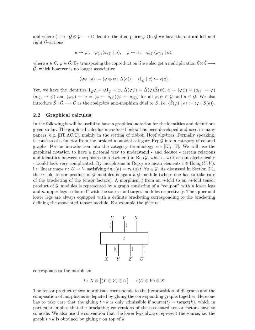
In the following it will be useful to have a graphical notation for the identities and definitionsgiven so far. The graphical calculus introduced below has been developed and used in manypapers, e.g. [RT,AC,T], mainly in the setting of ribbon–Hopf algebras. Formally speaking,it consists of a functor from the braided monoidal category RepG into a category of coloredgraphs. For an introduction into the category terminology see [K], [T]. We will use thegraphical notation to have a pictorial way to understand - and deduce - certain relationsand identities between morphisms (intertwiners) in RepG, which - written out algebraically- would look very complicated. By morphisms in Rep G we mean elements t ∈ HomG(U, V ),i.e. linear maps t : U → V satisfying t πU (a) = πV (a) t, ∀a ∈ G. As discussed in Section 2.1,the n–fold tensor product of G–modules is again a G–module (where one has to take careof the bracketing of the tensor factors). A morphism t from an n-fold to an m-fold tensorproduct of G–modules is represented by a graph consisting of a “coupon” with n lower legsand m upper legs “coloured” with the source and target modules respectively. The upper andlower legs are always equipped with a definite bracketing corresponding to the bracketingdefining the associated tensor module. For example the picture

X Y Z U

[( ) ]

t

U V X

( )

corresponds to the morphism

t : X ⊗[

(Y ⊗ Z) ⊗ U]

−→ (U ⊗ V ) ⊗X

The tensor product of two morphisms corresponds to the juxtaposition of diagrams and thecomposition of morphisms is depicted by gluing the corresponding graphs together. Here onehas to take care that the gluing t k is only admissible if source(t) = target(k), which inparticular implies that the bracketing conventions of the associated tensor factors have tocoincide. We also use the convention that the lower legs always represent the source, i.e. thegraph t k is obtained by gluing t on top of k.

8

Following the conventions of [AC] we now give a list of some special morphisms depictedby the following graphs:

V

:= idV ,

(2.29)

V ∗V:= bV

V ∗V

C

,

V∗V

:= aV

V∗V

C

(2.30)

@@

@@V W

W V

:= BV W ,@

@@

W V

V W

:= B−1V W

(2.31)

where C stands for the one dimensional representation given by the counit and where

bV : C −→ V ⊗ ∗V, 1 7−→∑

i

βV vi ⊗ vi

aV : ∗V ⊗ V −→ C, v ⊗ w 7−→ 〈v | αV w〉

BV W = τV W RV W , B−1V W = R−1

V W τWV .

Here vi is a basis of V with dual basis vi and τV W denotes the permutation of tensorfactors in V ⊗W . We also use the shortcut notation αV ≡ πV (α), RV W ≡ (πV ⊗ πW )(R),etc. The properties of G being a quasitriangular quasi-Hopf algebra ensure, that the abovedefined maps are in fact intertwiners (morphisms of G-modules). Note that within highertensor products the graphs (2.30) and (2.31) are only admissible if their legs are “bracketedtogether”. In order to change the bracket convention one has to use rebracketing morphisms.These are given as products of the basic elements

U V W

(

( )

)

= φUV W ,

U V W

(

( )

)

= φ−1UV W

(2.32)

where each of the three individual legs in (2.32) may again represent a tensor product ofG–modules. In this way we adopt the convention that any empty coupon with the samenumber of upper and lower legs - where the colouring only differs by the bracket convention- always represents the associated unique rebracketing morphism in RepG given in terms ofsuitable products of φ’s. We have already remarked that the uniqueness of this rebracketingmorphism (i.e. the independence of the chosen sequence of intermediate rebracketings) isguaranteed by McLanes coherence theorem and the “pentagon axiom” (2.2). This is why it

9

is often not even necessary to spell out one of the possible formulas for such an intertwiner.Explicitly, the pentagon identity (2.2) may be expressed as

( () )

[( ) ]

(

(

)

)[ ]

][

=

( () )

( )][

[( ) ]

(2.33)

which is the graphical notation for

(id ⊗ ∆ ⊗ id)(φ) (φ ⊗ 1) (∆ ⊗ id ⊗ id)(φ−1) = (1 ⊗ φ−1) (id ⊗ id ⊗ ∆)(φ)

In the same philosophy one may rewrite a simple rebracketing as a product of more compli-cated ones, as long as the overall source and target brackets coincide, for example

(

( )

)[

[

]

]

=( () )

[( ) ]

( () )

( )][

(2.34)

As done in the above pictures we will frequently not specify the modules sitting at thesource and target legs. Also note that by Eqs.(2.4) and (2.5) the rebracketing of the (in-visible) “white” leg corresponding to the trivial G–module C is always given by the trivialidentification.

If G is finite dimensional, it may itself be viewed as a G-module under left multiplicationand algebraic identities may directly be translated into identities of the corresponding graphsand vice versa. So e.g. Eq. (2.8) is equivalent to

(

( )

)

= =

(

( )

)

(2.35)

and Eqs. (2.4) and (2.5) together with (2.7) imply

[ ( )]

[( ])

=

[ ( )]

(2.36)

10

and

[ ( )]

( ( ))

=

[ ( )]

(2.37)

as well as the upside–down and left–right mirror images of (2.36) and (2.37) and the graphsobtained by rotating by 180 in the drawing plane. In general, with every graphical rule,where the graph is build from elementary graphs of the above list, the rotated as well as theupside–down and left–right mirror images are also valid and are proven analogously. Thisinduces a Z2 × Z2 - symmetry action on all graphical identities given below, which in factis already apparent in the axioms of a quasi–triangular quasi–Hopf algebra given in Section2.1 by taking Gop, Gcop or Gop

cop instead of G.Finally we point out the important “pull through” rule saying that morphisms built from

representation matrices of special elements in G (like the braiding (2.31) or the reassociator(2.32)) always “commute” with all other intertwiners in the appropriate sense i.e. by changingcolours and orderings accordingly. For example one has

X U

@@

@@

h

U V

=

X U

@@

@@

h

U V

,

(

(

)

)[ ]

][

h′

( )

=

h′

[ ( )]

(

( )

)

(2.38)

In the language of categories this means that the braidings and the reassociators providenatural transformations [ML].

2.3 The antipode image of the R–matrix

In this subsection we exploit the full power of our graphical machinery by proving variousimportant identities involving the action of the antipode on a quasitriangular R–matrix. Werecall that for ordinary Hopf algebras (i.e. where φ, α and β are trivial) one has (S⊗ id)(R) =R−1 = (id ⊗ S−1)(R) and (S ⊗ S)(R) = R. To generalize these identities to the quasi–Hopfcase we introduce the following four elements in G ⊗ G (using the notation (2.9))

pλ := Y i S−1(Xi β) ⊗ Zi pρ := P i ⊗Qi β S(Ri)

qλ := S(P i)αQi ⊗Ri qρ := Xi ⊗ S−1(αZi)Y i(2.39)

These elements have already been considered by [Dr2,S], see also Eqs. (9.20)-(9.23) of [HN].They obey the commutation relations (for all a ∈ G)

∆(a(2)) pλ [S−1(a(1)) ⊗ 1] = pλ [1 ⊗ a], ∆(a(1)) pρ [1 ⊗ S(a(2))] = pρ [a⊗ 1]

[S(a(1)) ⊗ 1] qλ ∆(a(2)) = [1 ⊗ a] qλ, [1 ⊗ S−1(a(2))] qρ ∆(a(1)) = [a⊗ 1] qρ(2.40)

see e.g. [HN,Lem. 9.1]. A graphical interpretation of these identities will be given in Eqs.(2.45) below. With these definitions we now have

11

Theorem 2.1. Let (G,∆, φ, S, α, β) be a finite dimensional quasi–Hopf algebra, let γ ∈ G⊗Gbe as in (2.18) and let R ∈ G ⊗ G be quasitriangular. Then

R−1 =[XjβS(P iY j) ⊗ 1] · [(S ⊗ id)(qopρ R)] · [(Ri ⊗Qi)∆op(Zj)]

=[∆(Rj) (Y i ⊗ Zi)] · [(id ⊗ S−1)(Rpρ)] · [1⊗ S−1(αQjXi)P j ] (2.41)

(S ⊗ S)(R) γ =γ21R (2.42)

A direct implication of equation (2.42) is the following formula, which has already beenstated without proof in [AC].

Corollary 2.2. Under the conditions of Theorem 2.1 let f ∈ G ⊗ G be the twist defined in(2.22), then

f opRf−1 = (S ⊗ S)(R) (2.43)

Proof of Corollary 2.2. Using the formula (2.22) for f and (2.42) one computes

f opR = (S ⊗ S)(∆(P i)) γop ∆op(QiβRi)R

= (S ⊗ S)(∆(P i)) (S ⊗ S)(R) γ∆(QiβRi)

= (S ⊗ S)(R) (S ⊗ S)(∆op(P i)) γ∆(QiβRi) = (S ⊗ S)(R) f.

To prepare the proof of Theorem 2.1 we need the following 3 Lemmata. First we have

Lemma 2.3.

( () )

( )][

[( ) ]

=

(2.44)

and three mirror images.

Proof. This is straightforward and left to the reader. (Use first (2.33), then (2.36) and (2.37)(or the suitable mirror image) and finally (2.35)).

To give an algebraic formulation of the four identities of Lemma 2.3 let us introduce thenotation

P λV W :=

(

( )

)

V ∗ V W

PρWV :=

(

( )

)

W V ∗V

QλV W :=

(

( )

)

∗V V W

QρWV :=

(

( )

)

W V V ∗

(2.45)

12

In a more general scenario these morphisms have already been introduced in [HN]. Alge-braically, they are given by (using the module notation)

P λV W : w 7→ vi ⊗ pλ · (vi ⊗ w), P

ρWV : w 7→ pρ · (w ⊗ vi) ⊗ vi, (2.46)

QλV W : v ⊗ v ⊗ w 7→ (v ⊗ id)

(

qλ · (v ⊗ w))

, QρWV : w ⊗ v ⊗ v 7→ (id ⊗ v)

(

qρ · (w ⊗ v))

see Eqs. (9.36),(9.37),(9.42) and (9.43) of [HN]. Note that the identities (2.40) precisely reflectthe fact that these maps are morphisms in RepG. In this way Lemma 2.3 is also containedin [HN, Lem 9.1], since it is equivalent to the four identities, respectively

[S(p1λ) ⊗ 1] qλ ∆(p2

λ) = 1 ⊗ 1, [1 ⊗ S−1(p2ρ)] qρ ∆(p1

ρ) = 1⊗ 1 (2.47)

∆(q2λ) pλ [S−1(q1λ) ⊗ 1] = 1 ⊗ 1, ∆(q1ρ) pρ [1 ⊗ S(q2ρ)] = 1⊗ 1.

Next we define intertwiners gV W : (∗W ⊗ ∗V ) ⊗ (V ⊗W ) → C and dV W : C → (V ⊗W ) ⊗(∗W ⊗ ∗V ) by

gV W :=

' $

( () )

[( ) ]

∗W ∗V V W

dV W :=

& %( () )

[( ) ]

V W ∗W ∗V

(2.48)

One directly verifies that

gV W (w ⊗ v ⊗ v ⊗ w) = 〈v ⊗ w| γV W (v ⊗ w)〉 (2.49)

dV W (1) =∑

i

(

δV W (vi ⊗ wi))

⊗(

wi ⊗ vi)

,

where v ∈ ∗V, w ∈ ∗W, v ∈ V, w ∈W and where vi⊗wi is a basis of V ⊗W with dual basisvi ⊗wi ∈ ∗V ⊗ ∗W . Here γ,δ ∈ G ⊗G are given in (2.18),(2.19) and γV W = (πV ⊗ πW )(γ),δV W = (πV ⊗ πW )(δ). We remark that in terms of these intertwiners the identities (2.25)may now be depicted as

∗(V ⊗W ) V ⊗W

' $=

∗(V ⊗W ) V ⊗W

f−1 idV ⊗W

( () )

gV W

;(V ⊗W )∗ V ⊗W

& %=

(V ⊗W )∗ V ⊗W

f idV ⊗W

( () )

dV ∗W ∗

(2.50)

Moreover, we have the following

Lemma 2.4.

gV W =

' $

( () )

( )][

∗W ∗V V W

dV W =

& %( () )

( )][

V W ∗W ∗V

(2.51)

13

Proof. We prove the first identity:

' $

( () )

[( ) ] ≡

( () )

( )][

[( ) ]

' $=

( () )

[( ) ]

(

(

)

)[ ]

][

' $

=

( () )

[( ) ]

[ ( )]

' $≡

( () )

( )][

' $

where in the second equality we have plugged in the pentagon identity (2.33) and in thethird we have used (2.36). The second identity in (2.51) is the upside–down mirror image ofthe first one and is proved analogously.

We invite the reader to check that algebraically Lemma 2.4 implies the following identitiesfor γ and δ defined in (2.18) and (2.19):

γ = (S(U i) ⊗ S(T i)) · (α ⊗ α) · (V i ⊗ W i)

δ = (Kj ⊗ Lj) · (β ⊗ β) · (S(N j) ⊗ S(M j)), where

T i ⊗ U i ⊗ V i ⊗ W i = (φ⊗ 1) · (∆ ⊗ id ⊗ id)(φ−1),

Kj ⊗ Lj ⊗ M j ⊗ N j = (id ⊗ id ⊗ ∆)(φ−1) · (1⊗ φ).

These identities have already been obtained by Drinfel’d [Dr2].Finally we note the following linear isomorphisms of intertwiner spaces holding in fact in

any rigid monoidal category.

Lemma 2.5. Let X,V,W be finite dimensional G-modules. Then there exist linear bijections

ΨVX,W : HomG(X ⊗W,V ) −→ HomG(X,V ⊗ ∗W ) (2.52)

ΦV,WX : HomG(X,V ⊗W ) −→ HomG(∗V ⊗X,W ) (2.53)

14

given by

ΨVX,W : h′

WX

V

7−→

h′

V

(

( )

)

X

∗W

;

(ΨVX,W )−1 : h

V ∗W

X

7−→

h

X

(

( )

)

V

W

ΦV,WX : h

V W

X

7−→

h

X

(

( )

)

W

∗V

;

(ΦV,WX )−1 : h′

X∗V

W

7−→

h′

W

(

( )

)X

V

Proof. We prove ΨVX,W (ΨV

X,W )−1 = id by determine its action on h ∈ HomG(X,V ⊗ ∗W )

15

as follows:

h

V ∗W

X

7−→h

(

( )

)

[ ]

[ ]

V ∗W

X(

( )

)

=

h

X

[ ]

( )

V ∗W

( () )

[( ) ]

= h

V ∗W

X

where in the first equality we have used a “pull through” rule for h, and in the secondequality a left–right mirror image of (2.44). Analogously one shows that Ψ−1 Ψ = id andΦ Φ−1 = id = Φ−1 Φ.

We are now in the position to prove Eqs. (2.41) and (2.42) of Theorem 2.1 by rewritingthem as graphical identities as follows:

Lemma 2.6. For all finite dimensional G-modules the inverse braiding B−1UV obeys

V U( () )

[( ) ]

@@

@@

( () )

[( ) ]

VU

=

V U

@@

@

VU

=

V U

VU

( () )

[( ) ]

@@

@@

( () )

[( ) ]

(2.54)

and the (left) conjugate braiding B∗U∗V obeys

∗U ∗V U V

@@

@@

( () )

[( ) ]

' $=

∗U ∗V U V

@@

@@

( () )

[( ) ]

' $

(2.55)

Taking G itself as a G-module yields (2.54) ⇔ (2.41) and (2.55) ⇔ (2.42) and therefore theabove identities prove Theorem 2.1.

16

Proof. To prove the first equation in (2.54) note, that (2.11) and (2.14) imply the identity

∗U U V

@@

@@

(

( )

)

@@

@@

(

( )

)

V

=

(

( )

)

∗U U V

(2.56)

Now we apply the isomorphism (ΦU,VU⊗V )−1 of Lemma 2.5 to both sides of (2.56) to obtain

U V

@@

@@

( () )

[( ) ]

@@

@@

[ ]

[ ]

(

( )

)

U V

≡

U V

@@

@@

( () )

( )][

(

( )

)

@@

@@

(

( )

)[ ]

[ ]

U V

=

U V( () )

( )][

(

( )

)

[ ]

[ ]

U V

(2.57)

where in the left identity we have used a “pull through” rule for the braiding. By the identity(2.37) the top of the graph in the middle of (2.57) may be replaced by

(

( )

)

[ ]

[ ]=

( () )

[( ) ]

,

(2.58)

17

and using Lemma 2.3 for the r.h.s. of (2.57) we end up with

U V

@@

@@

( () )

[( ) ]

@@

@@

( () )

[( ) ]

U V

=

U V

(2.59)

Hence we get the first equality in (2.54)7. Analogously one starts with (2.12),(2.14) to get

U V V ∗

@@

@@

(

( )

)

@@

@@

(

( )

)

U

=(

( )

)

U V V ∗

(2.60)

where we have used that the trivial identification ∗(V ∗) = V . Taking the mirror image of theabove proof yields the second equality in (2.54).

Eq. (2.55) follows from Lemma 2.7 below by putting h′ = BUV and h = B∗U∗V .The identifications (2.54) ⇔ (2.41) and (2.55) ⇔ (2.42) are straight forward and are left

to the reader. This concludes the proof of Lemma 2.6 and therefore also of Theorem 2.1.

We end this section with a Lemma used in the above proof, which will also be used in thenext section.

Lemma 2.7. Let V,W,X, Y be finite dimensional G–modules with intertwiners

h : ∗X ⊗ ∗Y −→ ∗W ⊗ ∗V, h′ : V ⊗W −→ Y ⊗X

7By finite dimensionality it suffices to prove the left inverse property.

18

then the following two identities are equivalent

∗X ∗Y V W

h

( () )

[( ) ]

' $

=

∗X ∗Y V W

h′

( () )

[( ) ]

' $

(2.61)

V∗Y( () )

[( ) ]

h

( () )

[( ) ]

∗WX

=

∗Y V

X ∗W

( () )

[( ) ]

h′

( () )

[( ) ]

=: H ′

∗Y V

X ∗W

(2.62)

Proof. Using (2.48), (2.51), a “pull through” rule for h and h′ and rebracketing the sourcelegs, Eq. (2.61) is equivalent to

∗X ∗Y V W

(

( )

)

[ ]

[ ]

h

(

( )

)

[ ]

' $

=

∗X ∗Y V W

(

(

)

)[ ]

][

h′

(

( )

)

' $[ ]

(2.63)

Note that the l.h.s. of (2.63) is of the form Ψ−1(· · · ) (with a “white” target leg). Now weapply the isomorphism ΨC

[∗X⊗(∗Y ⊗V )],W of Lemma 2.5 to both sides of (2.63). Then using for

19

the bottom part of the r.h.s. the identity

[ ( )]

(

(

)

)[ ]

][

=

( () )

( )][

)]

[ (

(2.64)

and a pull through rule to raise the upper box of the r.h.s. of (2.64) to the top we concludethat (2.63) is equivalent to

∗X ∗Y V

∗W

(

( )

)

h

(

( )

)

=

∗X ∗Y V

∗W

( () )

( )][

h′

(

( )

)

' $

[ ]

≡

∗X ∗Y V

∗W

H ′

( )

(

( )

)

(2.65)

The proof is finished by applying the isomorphism (Φ−1)X,∗W∗Y ⊗V .

3 Doubles of quasi-Hopf algebras

3.1 D(G) as an associative algebra

In this section we review the definition of the double D(G) of a quasi–Hopf algebra G as adiagonal crossed product as introduced in [HN]. We also give a graphical description of thisconstruction. Consider

δ := (∆ ⊗ id) ∆ : G −→ G ⊗ G ⊗ G (3.1)

and let Φ ∈ G⊗5

be given by

Φ := [(id ⊗ ∆ ⊗ id)(φ) ⊗ 1] [φ⊗ 1 ⊗ 1] [(δ ⊗ id ⊗ id)(φ−1)]. (3.2)

Then the pair (δ,Φ) provides a two–sided coaction of G on itself as defined in [HN], i.e thefollowing axioms are satisfied:

(i) The map δ is a unital algebra morphism satisfying (ǫ⊗ id ⊗ ǫ) δ = id.

20

(ii) The element Φ ∈ G⊗5

is invertible and fulfills

(id ⊗ δ ⊗ id)(δ(a))Φ = Φ (∆ ⊗ id ⊗ ∆)(δ(a)), ∀a ∈ G (3.3)

(1 ⊗ Φ ⊗ 1) (id ⊗ ∆ ⊗ id ⊗ ∆ ⊗ id)(Φ) (φ ⊗ 1⊗ φ−1)

= (id⊗2

⊗ δ ⊗ id⊗2

)(Φ) (∆ ⊗ id⊗3

⊗ ∆)(Φ) (3.4)

(id ⊗ ǫ⊗ id ⊗ ǫ⊗ id)(Φ) = (ǫ⊗ id⊗3

⊗ ǫ)(Φ) = 1 ⊗ 1⊗ 1 (3.5)

Next we define Ω ≡ Ω1 ⊗ Ω2 ⊗ Ω3 ⊗ Ω4 ⊗ Ω5 ∈ G⊗5

by8

Ω := (id⊗3

⊗ S−1 ⊗ S−1)(f45 · Φ−1) = (id⊗3

⊗ S−1 ⊗ S−1)(Φ−1) · h54 (3.6)

where f, h ∈ G ⊗ G are the twists defined in (2.22) and (2.27).Let now G be the coalgebra dual to G with its natural left and right G–action and the

nonassociative multiplication given by 〈ϕψ | a〉 := 〈ϕ ⊗ ψ | ∆(a)〉. With δ : G −→ G⊗3

being a two–sided coaction we then write ϕ⊲ a ⊳ψ := (ψ ⊗ id ⊗ ϕ)(δ(a)). Note that for thetwo–sided coaction δ in Eq. (3.1) we have the identity ϕ⊲ a ⊳ψ = (ϕ a) ψ. Consideredas an element of G we also write 1 ≡ 1G ≡ ǫ. The following proposition has been proven in[HN]:

Proposition 3.1. Let (δ,Φ) be a two–sided coaction of G on G and define the diagonalcrossed product G ⊲⊳ G to be the vector space G ⊗ G with multiplication rule

(ϕ ⊲⊳ a)(ψ ⊲⊳ b) :=[

(Ω1 ϕ Ω5)(Ω2 ψ(2) Ω4)]

⊲⊳[

Ω3(S−1(ψ(1)) ⊲ a ⊳ψ(3)) b]

,

(3.7)

where we write (ϕ ⊲⊳ a) in place of (ϕ⊗ a) to distinguish the new algebraic structure.Then G ⊲⊳ G is an associative algebra with unit 1 ⊲⊳ 1, containing G ≡ 1 ⊲⊳ G as a unital

subalgebra.

The associativity of the above product follows from the axioms for two–sided coactionsas has been proven in Theorem 10.2 of [HN]. Note that in general the subspace G ⊲⊳ 1 is not

a subalgebra of G ⊲⊳ G. On the other hand if G is an ordinary Hopf algebra with φ ≡ 1⊗1⊗1

then Eq. (3.7) becomes

(ϕ ⊲⊳ a)(ψ ⊲⊳ b) =(

ϕψ(2) ⊲⊳ (S−1(ψ(1)) ⊲ a ⊳ψ(3))b)

(3.8)

which is the standard multiplication rule in the quantum double D(G) [Dr1,M3]. This moti-vates the

Definition 3.2. [HN] The diagonal crossed product G ⊲⊳ G defined in Proposition 3.1, with(δ,Φ) given by (3.1),(3.2) is called the quantum double of G, denoted by D(G) ≡ G ⊲⊳ G.

We will now rewrite the multiplication (3.7) given in Proposition 3.1 using the “generatingmatrix” formalism of the St. Petersburg school. In this way we will be able to give a graphical(i.e. a categorical) description of the algebraic relations in G ⊲⊳ G which should convince thereader, that the multiplication given in (3.7) is indeed associative. The following Corollary isa generalization of [N, Lemma 5.2] and coincides with [HN,Cor. 10.4] applied to the presentscenario.

8 where we have again suppressed summation symbol and indices

21

Corollary 3.3. [HN] Let A be some unital algebra and γ : G −→ A a unital algebra map.Then the relation

γL(ϕ ⊲⊳ a) = (ϕ⊗ id)(L) · γ(a) (3.9)

provides a one to one correspondence between unital algebra morphisms γL : G ⊲⊳ G −→ Aextending γ and elements L ∈ G ⊗A satisfying (ǫ⊗ id)(L) = 1A and

[1G ⊗ γ(a)]L = [S−1(a(1)) ⊗ 1A]L [a(−1) ⊗ γ(a(0))], ∀a ∈ G (3.10)

L13L23 = [Ω5 ⊗ Ω4 ⊗ 1A][(∆ ⊗ id)(L)][Ω1 ⊗ Ω2 ⊗ γ(Ω3)], (3.11)

where Ω has been defined in (3.6) and where δ(a) ≡ a(−1) ⊗ a(0) ⊗ a(1).

An element L ∈ G ⊗ A satisfying (ǫ ⊗ id)(L) = 1A and (3.10/3.11) is called a normalcoherent (left diagonal) δ–implementer (with respect to γ), see [HN].

Note that by choosing A = G ⊲⊳ G and γ = id, Cor. 3.3 implies that the multiplicationon G ⊲⊳ G may uniquely be described by the relations of one “generating matrix” L =∑

eµ ⊗ (eµ ⊲⊳ 1), where eµ is a basis in G with dual basis eµ. In fact this formulation isused in [HN] to prove the associativity of the multiplication (3.7).

We now give a graphical interpretation of the identities (3.10),(3.11) by using that anyunital algebra map γ : G −→ A defines a G–module structure on A via b · A ≡ πA(b)A :=γ(b)A. Moreover, given two G–modules V,W then (V ⊗A)⊗W becomes a G–module by set-ting πV ⊗A⊗W (a) = (πV ⊗πA⊗πW )(δ(a)). Considering G as a G–module by left multiplicationwe now define the map

LA(G⊗A)⊗G∗ : (G ⊗ A) ⊗ G∗ −→ A, (b⊗A⊗ ϕ) 7→ (ϕ⊗ id)

(

L · (b⊗A))

Then Eq. (3.10) is equivalent to LA(G⊗A)⊗G∗ being an intertwiner of G–modules, i.e. to

LA(G⊗A)⊗G∗ ∈ HomG

(

(G ⊗ A) ⊗ G∗,G)

. We depict this intertwiner as

LA(G⊗A)⊗G∗ := L

G A G∗

A

( )

,

and call this a d–fork (≡ down fork) graph. The “coherence condition” (3.11) is now equivalentto the graphical identity

G G A G∗ G∗

L

[( ) ]

L

( )

A

=

G G A G∗ G∗

[( ) ] ( )

[( ) ]

idG⊗G f

L

( )

A

(3.12)

Note that the lowest box on the r.h.s. represents the rebracketing morphism Φ−1 defined in(3.2). This explains why one has to chose the complicated multiplication rule (3.7) insteadof (3.8) if φ and therefore f and Φ are non–trivial.

22

3.2 Coherent ∆–flip operators

We are now going to provide another set of generators in D(G) which later will be moreappropriate for defining the (quasitriangular) quasi–Hopf structure. Associated with anycoherent (left diagonal) δ–implementer L we define the element T ∈ G ⊗A by

T := [S−1(p2ρ) ⊗ 1] · L · (id ⊗ γ)(∆(p1

ρ)), (3.13)

where pρ ≡ p1ρ ⊗ p2

ρ has been given in (2.39).

Proposition 3.4. [HN] The relation (3.13) defines a one-to-one correspondence betweenelements L ∈ G ⊗A satisfying (3.10) and (3.11) and elements T ∈ G ⊗A satisfying

(id ⊗ γ)(∆op(a))T = T(id ⊗ γ)(∆(a)), ∀a ∈ G (3.14)

φ312A T13(φ−1)132A T23φA = (∆ ⊗ id)(T), (3.15)

where φA = (id ⊗ id ⊗ γ)(φ). L is recovered from T by

L = (id ⊗ γ)(qopρ )T (3.16)

Moreover (ǫ⊗ id)(T) = 1A if and only if (ǫ⊗ id)(L) = 1A.

Following [HN,Sect. 11] we call the elements T ∈ G ⊗ A satisfying (3.14) and (3.15)coherent ∆–flip operators. They are special versions of coherent λρ–intertwiners [HN, Def.10.8] associated with quasi–commuting pairs (λ, ρ) of left G–coactions λ and right G–coactionsρ on an algebra M. Proposition 3.4 has been proven algebraically in [HN,Prop. 10.10]. Beforegiving an alternative proof below, using the graphical calculus developed in Section 2.2 and2.3, let us state the following central consequence

Theorem 3.5. Define the element D ∈ G ⊗ (G ⊗ G) by9.

D :=∑

µ

S−1(p2ρ) eµ p

1ρ(1) ⊗ (eµ ⊗ p1

ρ(2)) (3.17)

and denote iD : G → G ⊗G the canonical embedding iD(a) := 1G⊗ a. Then there is a unique

algebra structure on the vector space G ⊗ G satisfying

iD(a)iD(b) = iD(ab) ∀a, b ∈ G (3.18)

D · (id ⊗ iD)(∆(a)) = (id ⊗ iD)(∆op(a)) ·D ∀a ∈ G (3.19)

φ312 D13(φ−1)132 D23φ = (∆ ⊗ id)(D). (3.20)

where we have identified φ ≡ (id ⊗ id ⊗ iD)(φ) ∈ G ⊗ G ⊗D(G). This algebra is precisely thequantum double D(G) defined in Prop. 3.1 and we have

ϕ ⊲⊳ a = (iD ⊗ ϕ(1))(qρ) (ϕ(2) ⊗ id)(D) iD(a) (3.21)

Proof. Follows from Proposition 3.4 and Cor. 3.3 by choosing A = D(G) which means thatT = D.

We call D the universal ∆–flip operator in D(G). The description of the quantum doubleD(G) as given in Theorem 3.5 will be used in the next section to derive the quasi–Hopfstructure of D(G). We now prove Proposition 3.4.

9as before eµ denotes a basis of G with dual basis eµ

23

Proof of Proposition 3.4. The equivalence (ǫ⊗ id)(T) = 1A ⇔ (ǫ⊗ id)(L) = 1A follows fromproperty (2.5) of φ. To show that the relations (3.10) and (3.11) for L are equivalent to therelations (3.14) and (3.15) for T, respectively, we use the graphical calculus. First we use theisomorphism ΨA

(G⊗A),G∗ of Lemma 2.5, to define the intertwiner TGA ∈ HomG(G ⊗A,A⊗G)by

TGA ≡

G A

q q q q q q q q q qGA

:=

G A

( () )

[( ) ]

L

GA

(3.22)

Algebraically Definition (3.22) translate into TGA(b⊗A) := T21 · (A⊗ b), where T ∈ G⊗A isexpressed in terms of L by (3.13). Now note that the property of TGA being an intertwiner ofG–modules is equivalent to T satisfying (3.14). Thus we have proven the equivalence (3.10) ⇔(3.14) and since the map ΨA

(G⊗A),G∗ is invertible also the invertibility of the transformation

(3.13). In fact, (3.16) is equivalent to

L

G A G∗

A

( )

=

G A G∗

q q q q q q q q q q(

( )

)

A

We are left to show that (3.11) ⇔ (3.15) (under the conditions (3.10) and (3.14), respec-tively). To this end we use that Eq. (3.15) is graphically expressed as

G G A

q q q q q q q q q q

(

( )

)

q q q q q q q q q qGGA

=

(

( )

)

G G A

idG⊗G

q q q q q q q q q q q q q q q

idG⊗G

(

( )

)GGA

(3.23)

Thus the following Lemma proves the equivalence (3.11) ⇔ (3.15) and therefore completesthe proof of Proposition 3.4

24

Lemma 3.6. The graphical identities (3.12) for LA(A⊗G)⊗G∗ and (3.23) for TGA are equiva-

lent.

Proof. Let us prove (3.12) ⇒ (3.23): Using the definition (3.22) we get for the l.h.s. of (3.23)

l.h.s =of (3.23)

( () )

[( ) ]

L

( )

@@

@( () )

[( ) ]

L

( )

=

( )]

[

( ) & %

L

[ [( ) ] ]

L

[( ) ]

Here we have used a pull through rule to push the lower d–fork up and then we havecombined all rebracketing morphisms in one box. Now plugging in Eq. (3.12), splitting the re-bracketing morphism at the bottom into four factors and pushing two of them up, one obtains

l.h.s. of (3.23) =

( )]

[

( ) & %

[(( ) ) ( )]

idG⊗G f

[( ) ]

L

=

(

( )

)

( () )

( )][

f idG⊗GidG⊗G

& %

( ) [ ]

[( ) ]

idG⊗GL

( )

( )

Using the identity (2.50) the last picture equals the r.h.s. of (3.23). Hence we have shown(3.12) ⇒ (3.23). The implication (3.23) ⇒ (3.12) is shown similarly by bending the two upperG–legs in (3.23) down again. Thus we have proved Lemma 3.6 and therefore also Proposition3.4.

25

3.3 Left and right diagonal crossed products

In this subsection we sketch how the quantum double D(G) may equivalently be modeled onG ⊗ G instead of G ⊗ G. (In fact this is true for any diagonal crossed product as has beenshown in [HN,Thm. 10.2].) With the notation as in Proposition 3.1 and with ΩR ∈ G⊗5

given

by ΩR := (h−1)21 · (S−1⊗S−1⊗ id⊗3

G )(Φ) the right diagonal crossed product G ⊲⊳ G is defined

to be the vector space G ⊗ G with multiplication rule

(a ⊲⊳ ϕ)(b ⊲⊳ ψ) :=[

a(

ϕ(1) ⊲ b ⊳ S−1(ϕ(3))

)

Ω3R

]

⊲⊳[

(Ω2R ϕ(2) Ω4

R)(Ω1R ψ Ω5

R)]

.

(3.24)

This makes G ⊲⊳ G an associative algebra with unit 1⊗ 1, containing G ≡ G ⊲⊳ 1 as a unitalsubalgebra. To see that the two algebras G ⊲⊳ G and G ⊲⊳ G are isomorphic let us begin withstating the analogue of Lemma 3.3: Let γ : G −→ A be a unital algebra map into some targetalgebra A. Then the relation

γR(a ⊲⊳ ϕ) = γ(a) · (ϕ⊗ id)(R) (3.25)

provides a one–to–one correspondence between unital algebra morphisms γR : G ⊲⊳ G −→ Aextending γ and elements R ∈ G ⊗A satisfying (ǫ⊗ id)(R) = 1A and

R [1G ⊗ γ(a)] = [a(1) ⊗ γ(a(0))]R [S−1(a(−1)) ⊗ 1A], ∀a ∈ G (3.26)

R13 R23 = [Ω4R ⊗ Ω5

R ⊗ γ(Ω3R)] (∆ ⊗ id)(R) [Ω2

R ⊗ Ω1R ⊗ 1A)] (3.27)

We call such elements normal coherent right diagonal δ–implementers [HN]. With this defi-nition one gets

Lemma 3.7. Let γ : G −→ A be some unital algebra map. Then the relation

R := [Φ5S−1(Φ4β) ⊗ 1A]L [Φ2S−1(Φ1β) ⊗ γ(Φ3)] (3.28)

defines a one–to–one correspondence between unital algebra maps γL : G ⊲⊳ G −→ A and uni-tal algebra maps γR : G ⊲⊳ G −→ A extending γ, as defined in (3.9) and (3.25), respectively.

Proof. We will sketch the proof, using graphical methods. For more details see [HN, Prop.

10.5]. Defining the map R(G∗⊗A)⊗GA : A −→ (G∗ ⊗A) ⊗ G by

R(G∗⊗A)⊗GA (A) :=

∑

eµ ⊗[

R21 · (A⊗ eµ)]

, A ∈ A,

property (3.26) of R is equivalent to R(G∗⊗A)⊗GA being an intertwiner of G–modules. Depicting

this intertwiner as a u–fork (≡ up fork) graph

R(G∗⊗A)⊗GA := R

G∗ A G

A

( )

,

26

the relation (3.28) may graphically be expressed as

R

G∗ A G

A

( )

:=

[( ) ] ( )

[( ) ]

A

L

G∗ A G

(3.29)

Since the r.h.s. of (3.29) defines a G–module intertwiner if and only if L satisfies (3.10),the element R defined by (3.28),(3.29) satisfies (3.26) if and only if L satisfies (3.10). Theequivalence of the coherence conditions (3.11) and (3.27) is shown by first expressing (3.27) asthe graphical identity (3.12), then plugging in the definition (3.29) and using a pull throughrule to collect all rebracketing morphisms at the bottom of the graph and finally using theidentities (2.50). We leave it to the reader to draw the corresponding pictures.

We are left to show that relation (3.28) may be inverted. This follows by a “two–sidedversion” of Lemma 2.5. The reader is invited to check that the inverse is given by

L := [S−1(αΦ5)Φ4 ⊗ γ(Φ3)]R [S−1(αΦ2)Φ1 ⊗ 1A], (3.30)

with Φ−1 =: Φ1 ⊗ Φ2 ⊗ Φ3 ⊗ Φ4 ⊗ Φ5. Eq. (3.30) may be expressed graphically as the up–side–down mirror image of picture (3.29) with L and R as well as G and G∗ exchanged.

Putting A = G ⊲⊳ G and γL = id or A = G ⊲⊳ G and γR = id, respectively, Lemma 3.7 implies

Corollary 3.8. Let (δ,Φ) be the two–sided coaction of G on G given in (3.2) and defineV ≡ V 1 ⊗ V 2 ⊗ V 3, W ≡W 1 ⊗W 2 ⊗W 3 ∈ G⊗3

by

V := S(Φ1)αΦ2 ⊗ Φ3 ⊗ S−1(αΦ5)Φ4, W := Φ2S−1(Φ1β) ⊗ Φ3 ⊗ Φ4βS(Φ5)

Then the map

G ⊲⊳ G ∋ (ϕ ⊲⊳ a) 7→(

V 2 ⊲⊳(

S−1(V 1) ϕ V 3)

)

· (a ⊲⊳ 1) ∈ G ⊲⊳ G

provides an algebra isomorphism with inverse given by

G ⊲⊳ G ∋ (a ⊲⊳ ϕ) 7→ (1 ⊲⊳ a) ·(

(

W 1 ϕ S−1(W 3))

⊲⊳ W 2)

∈ G ⊲⊳ G.

Corollary 3.8 has been proven for general diagonal crossed products in [HN, Thm. 10.2.iii]using the notation V ≡ qδ and W ≡ pδ. We also remark that one may equally well use thetwo–sided G–coaction δ′ := (id⊗∆) ∆ with reassociator Φ′ := [1⊗ (id⊗∆⊗ id)(φ−1)][1⊗1⊗ φ−1][(id ⊗ id ⊗ δ′)(φ)] to construct another to versions of quantum doubles G ⊲⊳δ′ G andG ⊲⊳δ′ G. Since the two–sided coactions (δ,Φ) and (δ′,Φ′) are twist equivalent [HN, Prop.8.4],these constructions are also isomorphic to the previous ones, i.e. all four diagonal crossedproducts define equivalent extensions of G [HN, Prop. 10.6].

3.4 The quasitriangular quasi–Hopf structure

In [HN] we have shown that D(G) is a quasi–bialgebra. As one might expect, D(G) is even aquasitriangular quasi-Hopf algebra. This is the content of the next theorem.

27

Theorem 3.9. Let D(G) be the associative algebra defined in Theorem 3.5. Then(D(G),∆D , ǫD, φD, SD, αD, βD, RD) is a quasitriangular quasi-Hopf algebra, where

φD :=(iD ⊗ iD ⊗ iD)(φ), (3.31)

RD :=(iD ⊗ id)(D) =∑

µ

iD(eµ) ⊗D(eµ) (3.32)

and where the structural maps are given by

∆D(iD(a)) := (iD ⊗ iD)(∆(a)), ∀a ∈ G (3.33)

(iD ⊗ ∆D)(D) := (φ−1D )231D13φ213

D D12φ−1D , (3.34)

ǫD(iD(a)) := ǫ(a), ∀a ∈ G, (3.35)

(id ⊗ ǫD)(D) := (ǫ⊗ id)(D) ≡ 1D(G). (3.36)

Furthermore the antipode SD is defined by

SD(iD(a)) := iD(S(a)), ∀a ∈ G (3.37)

(S ⊗ SD)(D) := (id ⊗ iD)(f op)D(id ⊗ iD) (f−1) (3.38)

where f ∈ G ⊗ G is the twist defined in (2.22). The elements αD, βD are given by

αD := iD(α), βD := iD(β). (3.39)

Proof. To simplify the notation we will frequently suppress the embedding iD, if no confusionis possible, i.e. we write α ≡ iD(α) = αD, (id⊗id⊗iD)(φ) ≡ φ etc. To show that (3.33),(3.34)define an algebra morphism ∆D : D(G) −→ D(G) ⊗ D(G), it is sufficient to check theconsistency with the defining relations (3.18) - (3.20). Consistency with (3.18) is obviousbecause of (3.33). Let us go on with (3.19): For the r.h.s. we get

(id ⊗ ∆D)(

∆op(a)D)

= [(∆ ⊗ id)(∆(a))]231 · (φ−1)231D13φ213D12φ−1

The l.h.s. yields

(id ⊗ ∆D)(

D ∆(a))

= (φ−1)231D13φ213D12φ−1[(id ⊗ ∆)(∆(a))],

which, using (3.19) and the property φ(∆ ⊗ id)(∆) = (id ⊗ ∆)(∆)φ to shift the factor(id ⊗ ∆)(∆(a)) to the left, equals the r.h.s..Consistency with the relation (3.20) may be checked in a longer but analogues calculation,where one also has to use the pentagon equation for φ several times, as in the proof of [HN,Lem. 11.2]. Hence ∆D is an algebra map. To show that ∆D is quasi-coassociative we computeby a similar calculation

(1 ⊗ φD) · (id ⊗ ∆D ⊗ id) (id ⊗ ∆D)(D) = (id ⊗ id ⊗ ∆D) (id ⊗ ∆D)(D) · (1 ⊗ φD),

by using again the pentagon equation for φ and the covariance property (3.19).The property of ǫD being a counit for ∆D follows directly from the fact that

(id⊗ ǫ⊗ id)(φ) = 1⊗1. Hence (D(G),∆D, ǫD, φD) is a quasi–bialgebra, see [HN, Thm. 11.3]for more details.

To show quasitriangularity we first note that the element RD = (iD ⊗ id)(D) fulfills(2.11) and (2.12) so to say by definition because of (3.20) and (3.34). The invertibility of RD

28

is equivalent to the invertibility of D which will be proved in Lemma 3.10 (i) below. We areleft to show that RD intertwines ∆D and ∆op

D , i.e.

∆opD (iD(a)) ·RD = RD · ∆D(iD(a)), ∀a ∈ G (3.40)

(id ⊗ ∆Dop)(D)) · R23

D = R23D · (id ⊗ ∆D)(D). (3.41)

Now Eq. (3.40) follows from (3.19). Hence we also get in D(G)⊗3

R12D · (∆D ⊗ id)(RD) = (∆op

D ⊗ id)(RD) ·R12D , (3.42)

which together with (2.11) implies the quasi-Yang Baxter equation

(φ−1D )321R12

D φ312D R13

D (φ−1D )132 R23

D = R23D (φ−1

D )231 R13D φ213

D R12D φ−1

D . (3.43)

Using the Definition (3.34), Eq. (3.43) is further equivalent to

(iD ⊗ ∆opD )(D) ·R23

D = R23D · (iD ⊗ ∆D)(D)

which also proves (3.41). Hence RD is quasitriangular.

In order to prove that the definition of SD in (3.37),(3.38) may be extended anti-multiplicatively to the entire algebra D(G), we have to show that this continuation is con-sistent with the defining relations (3.19),(3.20). This amounts to showing

(S ⊗ SD)(D) · (S ⊗ SD)(∆op(a)) = (S ⊗ SD)(∆(a)) · (S ⊗ SD)(D), and (3.44)

(S ⊗ S ⊗ SD)(

(∆ ⊗ id)(D))

= (S ⊗ S ⊗ SD)(φ) · (S ⊗ S ⊗ SD)(D23)

· (S ⊗ S ⊗ SD)((φ−1)132) · (S ⊗ S ⊗ SD)(D13) · (S ⊗ S ⊗ SD)(φ312). (3.45)

Since by definition (S ⊗ SD)(D) = f opDf−1 10, equation (3.44) follows directly from (3.19)and the fact, that by (2.24) f has the property f ·∆(S(a)) = (S⊗S)(∆op(a))·f . For the proofof (3.45) let us recall, that ∆f := f∆(·)f−1 defines a twist equivalent quasi-coassociativecoproduct on G with twisted reassociator φf defined in (2.16) satisfying φf = (S⊗S⊗S)(φ321)(see (2.26)). Thus we get for the l.h.s. of (3.45) (with Df := f opDf−1)

(S ⊗ S ⊗ SD)(

(∆ ⊗ id)(D))

= (∆fop ⊗ id)

(

(S ⊗ SD)(D))

= (∆fop ⊗ id)(Df )

= φ321f D23

f (φ−1f )231D13

f φ213f ,

where the last equality is exactly the transformation property of a quasitriangular R-matrixunder a twist [Dr2] and may be proven analogously using (3.19). By (2.26) this equals ther.h.s. of (3.45). Hence SD defines an anti-algebra morphism on D(G).

We are left to show that the map SD fulfills the antipode axioms given in (2.7) and (2.8).Axiom (2.8) is clearly fulfilled since we have SD iD = iD S and αD = iD(α), βD = iD(β),φD = (iD ⊗ iD ⊗ iD)(φ). Noting that ∆D(iD(a)) = (iD ⊗ iD)(∆(a)) , a ∈ G, the validity ofaxiom (2.7) follows from its validity in G and Lemma 3.10 (ii) below.

10where we have again suppressed the embedding id ⊗ iD of f

29

Lemma 3.10.

(i) The universal flip operator D ∈ G ⊗ D(G) is invertible where the inverse is given by

D−1 = [XjβS(P iY j) ⊗ 1] · [(S ⊗ id)(qopρ D)] · [(Ri ⊗Qi)∆op(Z

j)], (3.46)

where qρ ∈ G ⊗ G has been defined in (2.39).

(ii) Let µD denote the multiplication map µD : D(G) ⊗D(G) −→ D(G), then

(id ⊗ µD) (id ⊗ SD ⊗ id)(

(id ⊗ ∆D)(D) · (1G ⊗ 1G ⊗ αD))

= 1G ⊗ αD (3.47)

(id ⊗ µD) (id ⊗ id ⊗ SD)(

(id ⊗ ∆D)(D) · (1G ⊗ βD ⊗ 1G))

= 1G ⊗ βD (3.48)

Proof. We will use the graphical methods adopted in Sections 2.2/2.3. To this end let usview G and D ≡ D(G) as left G–modules. Then, due to (3.19), BGD := τGD D defines anintertwiner BGD : G ⊗D −→ D ⊗ G which will be depicted as

BGD =:

G D

D G

q q q q q q q q q q

(In fact this is the intertwiner TGA defined in (3.22) for the special case A = D). For theleft modules ∗G and ∗D the corresponding intertwiners B∗GD, BG∗D, B∗G∗D are defined withthe help of the map S and/or SD. Graphically they are represented by the same picture,except that the colours of the legs are replaced by ∗G and(or) ∗D, respectively. The reasonfor distinguishing the D–line from the G–line lies in the fact that unlike in (2.31) BGD is not

given in terms of a quasitriangular R–matrix in G⊗G, which is why we write BGD in place ofBGD. Correspondingly, the identities derived in Section 2.3 are not automatically valid forBGD. We now show, which of them still hold. First, since S is an antipode for ∆, Eq. (3.20)together with (ǫ⊗ id)(D) = 1D implies the equality (compare with (2.56))

∗G G D

q q q q q q q q q q

(

( )

)

q q q q q q q q q q(

( )

)

D

=

(

( )

)

∗G G D

(3.49)

30

and a step by step repetition of the prove of (2.59) yields

(BGD)−1 =:

D Gq q q q q q q q

q q@@

@

DG

=

D G( () )

[( ) ]

q q q q q q q q q q

( () )

[( ) ]

DG

(3.50)

This means that algebraically we get the analogue of the first identity in Eq. (2.41) whichyields (3.46). Thus we have proven part (i)

To prove (ii) let us translate the two claims (3.47) and (3.48) into the graphical languageas

(3.47) ⇔

G D∗D

q q q q q q q q q q(

( )

)

q q q q q q q q q q

(

( )

)

G

=(

( )

)

G ∗D D

(3.51)

and

(3.48) ⇔

G

(

( )

)

q q q q q q q q q q

(

( )

)

q q q q q q q q q q

∗DD G

=(

( )

)

GD ∗D

(3.52)

Note that as opposed to (3.49) the identities (3.51) and (3.52) are not automatically satisfied,since SD is not yet proved to be an antipode for ∆D. To prove (3.51) and (3.52) we now

31

proceed backwards along the proof of Lemma 2.6, i.e. we use Lemma 2.5 to show that eitherof these two identities is equivalent to

∗D G( () )

[( ) ]

q q q q q q q q q q

( () )

[( ) ]

G ∗D

= q q q q q q q qq q@

@@

∗D G

:= (BG∗D)−1

(3.53)

More precisely (3.51) is equivalent to (3.53) just as (2.60) is equivalent to the second equationin (2.54), and “rotating” this proof by 180 in the drawing plane we also get (3.52) ⇔ (3.53).Thus we are left with proving (3.53). To this end we remark, that (3.49) equally holds if wereplace D by ∗D, and therefore (3.50) also holds with D replaced by ∗D. Hence (3.53) followsfrom (3.50) provided we can show

∗D G( () )

[( ) ]

q q q q q q q q q q

( () )

[( ) ]

G ∗D

=

∗D G( () )

[( ) ]

q q q q q q q q q q

( () )

[( ) ]

∗DG

(3.54)

By Lemma 2.7 this further equivalent to

∗G ∗D G D

q q q q q q q q q q( () )

[( ) ]

' $=

∗G ∗D G D

q q q q q q q q q q( () )

[( ) ]

' $

(3.55)

Using (2.48) and (2.49), Eq. (3.55) is algebraically equivalent to

γop D = (S ⊗ SD)(D) γ,

which finally holds by (3.38),(3.19) and (2.25). This concludes the proof of Lemma 3.10 (ii)and therefore of Theorem 3.9.

32

Clearly, if G is a Hopf algebra and φ = 1⊗1⊗1, one recovers the well-known definitionsof ∆D, SD and RD in Drinfelds quantum double

∆D(iD(g)) = (iD ⊗ iD)(∆(g))

∆D(D(ϕ)) = (D ⊗D)(∆op(ϕ))

SD(iD(g)) = iD(S(g))

SD(D(ϕ)) = D(S−1(ϕ))

RD = (1 ⊗ eµ) ⊗ (eµ ⊗ 1),

whereD(ϕ) := (ϕ⊗id)(D), ϕ ∈ G. As in the Hopf algebra case, one may take the constructionof the quasitriangular R-Matrix in D(G) as the starting point and formulate Theorem 3.5together with Theorem 3.9 differently:

Corollary 3.11. Let G be a finite dimensional quasi-Hopf algebra with invertible antipode.Then there exists a unique quasi-Hopf algebra D(G) such that

(i) D(G) = G ⊗ G as a vector space,

(ii) the canonical embedding iD : G → 1G ⊗ G ⊂ D(G) is a unital injective homomorphismof quasi-Hopf algebras,

(iii) Let D ∈ G ⊗ D(G) be given by Eq. (3.17), then the element RD := (iD ⊗ id)(D) ∈D(G) ⊗D(G) is quasitriangular.

This quasi–Hopf algebra structure is given by the definitions in Theorem 3.5 and 3.9.

Proof. The property (ii) implies (3.18), (3.33), (3.31), (3.35) and (3.39), yielding also fD =(iD ⊗ iD)(f). The quasitriangularity of RD implies (3.19), (3.20), (3.34) and (3.36) andaccording to (2.43) (SD ⊗ SD)(RD) = f

opD RDf

−1D . Hence the antipode is uniquely fixed to

be the one defined in Theorem 3.9.

We are now in the position to prove Theorem A.

Proof of Theorem A. First note that Corollary 3.11 already proves the existence parts (i),(ii)of Theorem A by putting D(ϕ) := (ϕ ⊗ id)(D). The fact that µ : G ⊗ G −→ D(G) providesa linear isomorphism follows from the last statement in Theorem 3.5. Moreover, if D ⊃ Gis another Hopf algebra extension and if D : G −→ D is a linear map such that D isalgebraically generated by G and D(G) and RD := eµ ⊗ D(eµ) ∈ D ⊗ D is quasitriangular,

then ν : D(G) −→ D

ν(ϕ⊗ a) := (id ⊗ ϕ(1))(qρ) D(ϕ(2)) a (3.56)

is a uniquely and well defined algebra map satisfying ν D = D by Prop. 3.4. In fact, thequasitriangularity of RD implies that ν is even a quasi–bialgebra homomorphism. Thus D(G)also solves the universality property (iii) of Theorem A. In particular the extension D(G) ⊃ Gis unique up to equivalence.

3.5 The category RepD(G)

We will now give a representation theoretical interpretation of the quantum double D(G)by describing its representation category in terms of the representation category of the un-derlying quasi-Hopf algebra G. In this way we will show that D(G) is a concrete realizationof the quantum double as defined by Majid in [M2] with the help of a Tannaka-Krein-like

33

reconstruction theorem. We denote the monoidal category of finite dimensional unital rep-resentations of D(G) and of G by RepD(G) and RepG, respectively. The next propositionstates a necessary and sufficient condition, under which a representation of G extends to arepresentation of D(G):

Proposition 3.12.

1.) The objects of RepD(G) are in one to one correspondence with pairs (πV , V ),DV ,where (πV , V ) is a finite dimensional representation of G and where DV ∈ G ⊗ EndC(V ) isa normal coherent ∆-flip, i.e.

(i) (ǫ⊗ id)(DV ) = idV

(ii) DV · (id ⊗ πV )(∆(a)) = (id ⊗ πV )(∆op(a)) ·DV , ∀a ∈ G

(iii) φ312V D13

V (φ−1V )132 D23

V φV = (∆ ⊗ id)(DV ), where φV := (id ⊗ id ⊗ πV )(φ).

2.) Let (πV , V ),DV and (πW ,W ),DW be as above, then

HomD(G) =

t ∈ HomG(V,W ) | (id ⊗ t)(DV ) = DW

Proof. We define the extended representation πDV on the generators of D(G) by

πDV (iD(g)) : = πV (g), g ∈ G (3.57)

πDV (D(ϕ)) : = (ϕ⊗ idEndV

)(DV ), ϕ ∈ G (3.58)

Condition (i) implies that πDV is unital whereas conditions (ii),(iii) just reflect the defining

relations (3.19) and (3.20) of D(G), which ensures, that πDV is a well defined algebra morphism.

On the other hand, given a representation (πDV , V ) of D(G), we define

DV := (idG ⊗ πDV )(D)

which clearly satisfies conditions (i) - (iii). This proves part 1. Part 2. follows trivially.

To get the relation with Majid’s formalism [M2] we now write a · v := πV (a)v, a ∈ G, v ∈ V

and define βV : V −→ G ⊗ V ; v 7→ v(1) ⊗ v(2) := DV

(

1G ⊗ v)

. With this notation we getthe following Corollary:

Corollary 3.13. The conditions (i)-(iii) of Proposition 3.12 are equivalent to the followingthree conditions for βV (as before denoting P i ⊗Qi ⊗Ri = φ−1):

(i’) (ǫ⊗ idV ) βV = idV

(ii’) (a(2) · v)(1)a(1) ⊗ (a(2) · v)

(2) = a(2)v(1) ⊗ a(1) · v

(2), ∀v ∈ V

(iii’) Riv(1) ⊗ (Qi · v(2))(1) P i ⊗ (Qi · v(2))(2) =

(φ−1)321 ·[

(Ri · v)(1)(2)Q

i ⊗ (Ri · v)(1)(1) P

i ⊗ (Ri · v)(2)]

, ∀v ∈ V

Proof. The equivalences (i) ⇔ (i’) and (ii) ⇔ (ii’) are obvious. The equivalence (iii) ⇔ (iii’)follows by multiplying (iii) with (φ−1

V )312 from the left and with φ−1V from the right and

permuting the first two tensor factors.

The conditions stated in the above Corollary agree with those formulated in [M2, Prop.2.2]by taking Gcop ≡ (G,∆op, (φ−1)321) instead of (G,∆, φ) as the underlying quasi-bialgebra.This means that we have identified the category RepD(G) with what is called the doublecategory of modules over G in [M2].

34

4 Doubles of weak quasi–Hopf algebras

Allowing the coproduct ∆ to be non–unital (i.e. ∆(1) 6= 1 ⊗ 1) leads to the definition ofweak quasi–Hopf algebras as introduced by G. Mack and V. Schomerus in [MS]. In thisSection we sketch how the construction of the quantum double D(G) generalizes to this case.As it will turn out, there are only minor adjustments to be made. The reason for this liesin the fact, that we have used mostly graphical identities (i.e. identities in RepG) to deriveand describe our results. But since RepG is a rigid monoidal category also in the case ofweak quasi–Hopf algebras G, all graphical identities in Section 2.2 and 2.3 stay valid. Thusthe only adjustements required refer to those points, where we have translated graphicalidentities into algebraic ones.

Following [MS] we define a weak quasi–Hopf algebra (G,1,∆, ǫ, φ) to be an associativealgebra G with unit 1, a non–unital algebra map ∆ : G −→ G⊗G, an algebra map ǫ : G −→ C

and an element φ ∈ G ⊗ G ⊗ G satisfying (2.1)-(2.3), whereas (2.4) is replaced by

(id ⊗ ǫ⊗ id)(φ) = ∆(1) (4.1)

and where in place of invertibility φ is supposed to have a quasi–inverse φ ≡ φ−1 with respectto the intertwining property (2.1). By this we mean that φ satisfies φφφ = φ, φφφ = φ aswell as

φ φ = (id ⊗ ∆)(∆(1)), φ φ = (∆ ⊗ id)(∆(1)) (4.2)

which implies the further identities

(id ⊗ ∆)(∆(a)) = φ (∆ ⊗ id)(∆(a)) φ, ∀a ∈ G (4.3)

φ = φ (∆ ⊗ id)(∆(1)), φ = φ (id ⊗ ∆)(∆(1)) (4.4)

(id ⊗ ǫ⊗ id)(φ) = ∆(1) (4.5)

More generally we call an element t ∈ A an intertwiner between two (possibly non–unital)algebra maps α, β : G −→ A, if

t α(a) = β(a) t, ∀a ∈ G and t α(1) ≡ β(1) t = t

In this case by a quasi–inverse of t (with respect to this intertwiner property) we mean theunique (if existing) element t ≡ t−1 ∈ A satisfying tt = α(1), tt = β(1) and ttt = t. Notethat this implies

t β(a) = α(a) t, t β(1) ≡ α(1) t = t

and therefore t is also the quasi–inverse of t−1.A weak quasi–bialgebra is called weak quasi–Hopf algebra, if there exists a unital algebra

antimorphism S : G −→ G and elements α, β ∈ G satisfying (2.7) and (2.8). We will alsoalways suppose that S is invertible.

Furthermore, G is said to be quasitriangular if there exists an element R ∈ G ⊗ G satis-fying (2.10)–(2.12) and possessing a quasi–inverse R ≡ R−1 with respect to the intertwiningproperty (2.10).

With these substitutions Theorem A generalizes as follows

Theorem B Let (G,∆, φ) be a finite dimensional weak quasi–Hopf algebra with invertibleantipode S. Assume D(G) ⊃ G to be a weak quasi–Hopf algebra extension satisfying (i)-(iii)

35

of Theorem A. Then D(G) exists uniquely up to equivalence and the linear map µ : G ⊗G −→D(G)

µ(ϕ⊗ a) := (id ⊗ ϕ(1))(qρ)D(ϕ(2))

is surjective with Kerµ = KerP , where P : G ⊗ G −→ G ⊗ G is the linear projection

P (ϕ⊗ a) := ϕ(2) ⊗(

(

S−1(ϕ(1)) 1G

)

ϕ(3)

)

a =: ϕ ⊲⊳ a

To adapt our previous strategy to weak quasi–Hopf algebras we first recall that due tothe coproduct being non–unital the definition of the tensor product functor in RepG hasto be slightly modified. First note that the element ∆(1) (as well as higher coproducts of1) is idempotent and commutes with all elements in ∆(G). Thus, given two representations(V, πV ), (W,πW ), the operator (πV ⊗ πW )(∆(1)) is a projector, whose image is precisely theG–invariant subspace of V ⊗W on which the tensor product representation operates nontrivial. Thus one is led to define the tensor product ⊠ of two representations of G by setting

V ⊠W := (πV ⊗ πW )(∆(1)) (V ⊗W ), πV ⊠ πW := (πV ⊗ πW ) ∆|V ⊠W (4.6)

One readily verifies that with these definitions φUV W - restricted to the subspace (U⊠V )⊠W- furnish a natural family of isomorphisms defining an associativity constraint for the tensorproduct functor ⊠, where the tensor product of morphisms is defined by restricting the“usual” tensor product map to the truncated subspace.

With these adjustments, the graphical calculus described in Section 2.2 and 2.3 carriesover to the present case. The collection of colored upper (or lower) legs represent the (trun-cated) tensor product of G–modules associated with the individual legs. One just has to takecare when translating the pictures into algebraic identities. For example the graph

G G

≡

G ⊠ G

is a pictorial representation of ∆(1) and not of 1 ⊗ 1! Thus the graph (2.44) is equivalentto the algebraic identity [S(p1

λ)⊗ 1] qλ ∆(p2λ) = ∆(1) in place of the first equation of (2.47),

etc. In this way all graphical identities of Section 2 stay valid as well as Theorem 2.1, wherenow R−1 is meant to be the quasi–inverse of R.

The definition of the diagonal crossed product in Proposition 3.1 yields an associativealgebra which in general is not unital, but (1

G⊗ 1G) is still a right unit and in particular

idempotent [HN, Thm. 14.2]. This may be cured by taking the right ideal generated by(1

G⊗1G). Thus, let P : G ⊗G −→ G ⊗G be the linear projection given by left multiplication

with 1G⊗ 1G with respect to the algebra structure (3.7), i.e.

P (ϕ⊗ a) := ϕ(2) ⊗(

S−1(ϕ(1)) ⊲1 ⊳ϕ(3)

)

a = 1(−1) ϕ S−1(1(1)) ⊗ 1(0) a. (4.7)

As in [HN, Sect. 14] we introduce the notation

ϕ ⊲⊳ a := P (ϕ⊗ a) ∈ G ⊗ G (4.8)

and define the quantum double D(G) as the subalgebra

D(G) := G ⊲⊳ G ≡ P (G ⊗ G) (4.9)

36

Then 1G⊲⊳ 1G ≡ 1

G⊗ 1G is the unit of D(G) and in terms of the notation (4.8) the

multiplication in D(G) is still given by (3.7). In particular

iD : G ∋ a 7→ 1G⊲⊳ a ≡ 1

G⊗ a ∈ D(G)

still provides a unital algebra inclusion. Interpreting Eq. (3.9) also via (4.8), Corollary 3.3likewise extends to the present scenario. However note that now the definition (3.10) for leftdiagonal δ–implementers L ∈ G ⊗A also implies the nontrivial relation

L ≡ [1G ⊗ 1A]L = [S−1(1(1)) ⊗ 1A]L [1(−1) ⊗ τ(1(0))], (4.10)

This leads to a slight modification of Proposition 3.4 where one has to add the requirementthat ∆–flip operators T fulfill also

T (id ⊗ τ)(∆(1)) ≡ (id ⊗ τ)(∆op(1))T = T

which follows directly from (4.10) or by multiplicating both sides of (3.13) from the rightwith (id ⊗ τ)(∆(1)).

Taking this additional identity into account, Theorem 3.5 now reads

Theorem 4.1. Using the notation (4.8) we define the element D ∈ G ⊗ D(G) by

D :=∑

µ

S−1(p2ρ) eµ p

1ρ(1) ⊗ (eµ ⊲⊳ p1

ρ(2))

Then the multiplication (3.7) is the unique algebra structure on D(G) satisfying (3.18)–(3.20)together with

D (id ⊗ iD)(∆(1)) ≡ (id ⊗ iD)(∆op(1))D = D (4.11)

Moreover the identity (3.21) also stays valid.

The quasitriangular quasi–Hopf structure is now defined precisely as in Theorem 3.9 andis proven analogously, where in (3.38) f−1 is the quasi–inverse of f . Correspondingly D−1

given by (3.46) becomes the quasi–inverse of D with respect to the ∆–flip property (3.19).Thus we arrive at a

Proof of Theorem B. The existence parts (i),(ii) of Theorem B follow by putting as beforeD(ϕ) = (ϕ⊗ id)(D). The universality (and therefore uniqueness) property (iii) follows anal-ogously as in the proof of Theorem A, Eq. (3.56). Here one just has to note that by Prop. 3.4

L := qopρ D ∈ G ⊗ D

is a normal coherent δ–implementer, where D :=∑

eµ ⊗ D(eµ). Hence L satisfies (4.10) andtherefore the map ν : G ⊗ G −→ D

ν(ϕ⊗ a) := (ϕ⊗ id)(L) a

satisfies ν P = ν, where P is the projection (4.7). Since as in Corollary 3.3 the relations(3.10),(3.11) guarantee that ν is an algebra map with respect to the multiplication (3.7) onG ⊗ G, it passes down to a well defined algebra map f : D(G) −→ D, f(ϕ ⊲⊳ a) := ν(ϕ⊗ a),thus proving (iii). Since D (as an element in D ⊗ D) is also required to be quasitriangular,f is even a quasi–bialgebra homomorphism. In the case D = D(G) we have ν = µ andKerP = Kerµ by definition, proving also the second part of Theorem B.

37

A The twisted double of a finite group

As an application we now use Theorem 3.5 and Theorem 3.9 to recover the “twisted” quantumdouble Dω(G) of [DPR] where G is a finite group and ω : G×G×G→ U(1) is a normalized 3-cocycle. By definition this means ω(g, h, k) = 1 whenever at least one of the three argumentsis equal to the unit e of G and

ω(g, x, y)ω(gx, y, z)−1ω(g, xy, z)ω(g, x, yz)−1ω(x, y, z) = 1, ∀g, x, y, z ∈ G.

The Hopf algebra G := Fun(G) of functions on G may then also be viewed as a quasi-Hopfalgebra with its standard coproduct, counit and antipode but with reassociator given by

φ :=∑

g,h,k∈G

ω(g, h, k) · (δg ⊗ δh ⊗ δk), (A.1)

where δg(x) := δg,x. The identities (2.2) and (2.4) for φ are equivalent to ω being anormalized 3-cocycle. Also note that choosing α = 1G the antipode axioms now requireβ =

∑

g ω(g−1, g, g−1)δg. In this special example our quantum double D(G) ≡ G ⊲⊳ G allows

for another identification with the linear space G ⊗ G.

Lemma A.1. Let G be as above and define σ : G ⊗ G −→ D(G) by σ(ϕ⊗ a) := D(ϕ) a, ϕ ∈G, a ∈ G. Then σ is a linear bijection.

Proof. Since (G,∆, ǫ, S) is also an ordinary Hopf algebra, the relation (3.19) is equivalent to(suppressing the symbol iD)

aD(ϕ) = D(

a(1) ϕ S−1(a(3)))

a(2), ∀a ∈ G, ϕ ∈ G. (A.2)

Using (3.21) this implies

ϕ ⊲⊳ a ≡ (id ⊗ ϕ(1))(qρ)D(ϕ(2)) a = D(

q1ρ(1) ϕ (q2ρ S−1(q1ρ(3)))

)

q1ρ(2) a,

which lies in the image of σ. Hence, σ is surjective and therefore also injective.

We note that in general the map σ need not be surjective (nor injective). Due to Lemma A.1we may now identify D(G) with the new algebraic structure on G ⊗ G induced by σ−1. Wecall this algebra G ⊗D G. Putting a ≡ 1⊗D a, a ∈ G and D := eµ ⊗ (eµ ⊗D 1) ∈ G ⊗ (G ⊗D G)it is described by the relations (A.2),(3.20) and the requirement of G ≡ 1⊗DG being a unitalsubalgebra. To compute these multiplication rules we now use that the group elements g ∈ G

provide a basis in G with dual basis δg ∈ G. Hence a basis of G⊗DG is given by h⊗Dδgh,g∈G .In this basis the generating matrix D is given by

D =∑

k∈G

δk ⊗ (k ⊗D 1G), 1G =∑

h∈G

δh. (A.3)

Let us know compute the multiplication laws according to the definitions in Theorem 3.5.To begin with, we have

(h⊗ 1G)(e ⊗ δg) = (h⊗ δg) and (g ⊗ 1G)(h⊗ 1G) = (gh⊗ 1G).

Taking (x⊗ id) of both sides of (3.19), where x ∈ G, and using ∆(δg) =∑

k∈G δk ⊗ δk−1g weget

(x⊗ 1G)(e⊗ δx−1g) = (e⊗ δgx−1)(x⊗ 1G),

38

or equivalently

(e⊗ δg)(x⊗ 1G) = (x⊗ δx−1gx). (A.4)

Finally, pairing equation (3.20) with x ⊗ y ∈ G ⊗ G in the two auxiliary spaces, the l.h.s.yields

∑

s,r,t∈G

ω(s, x, y)(1 ⊗ δs)(x⊗ 1G) · ω(x, r, y)−1(e⊗ δr)(y ⊗ 1G) · ω(x, y, t)(1 ⊗ δt)

= (x⊗ 1G)(y ⊗ 1G) ·∑

s,r,t∈G

ω(s, x, y)ω(x, y, t)

ω(x, r, y)(e⊗ δ(xy)−1sxyδy−1ryδt)

=∑

t∈G

(x⊗ 1G)(y ⊗ 1G)(1 ⊗ δt)ω(xyt(xy)−1, x, y)ω(x, y, t)

ω(x, yty−1, y),

where we have used (A.4) in the first equality. The right hand side of (3.20) gives (xy ⊗ 1G)so that we end up with

(x⊗ 1G)(y ⊗ 1G) =∑

t∈G

ω(x, yty−1, y)

ω(xyt(xy)−1, x, y)ω(x, y, t)(xy ⊗ δt). (A.5)

Similarly the coproduct is computed as ∆D(e⊗ δg) =∑

k∈G(e⊗ δk) ⊗ (e⊗ δk−1g) and

∆D(x⊗ 1G) =∑

r,s∈G

ω(xrx−1, x, s)

w(x, r, s)ω(xrx−1, xsx−1, x)

(

(x⊗ δr) ⊗ (x⊗ δs))

. (A.6)

The above construction agrees with the definition of Dω(G) given in [DPR] up to the con-vention, that they have build D(G) on G ⊗ G instead of G ⊗ G.

B The Monodromy Algebra

The definition of monodromy algebras (see e.g. [AFFS]) associated with quasitriangular Hopfalgebras may now easily be generalized to the case of quasi-Hopf algebras. This has alreadybeen done in [AGS]. We will give an explicit proof that the defining relations of [AGS] indeeddefine an associative algebra structure on G ⊗G, which in fact is isomorphic to our quantumdouble D(G). For ordinary Hopf algebras this has recently been shown in [N1].

Let G be a finite dimensional quasi-Hopf algebra with quasitriangular R-matrix R ∈ G⊗G.Following [N1] we define the monodromy matrix M ∈ G ⊗ D(G) to be

M := (id ⊗ iD)(Rop)D.

Defining also R ∈ G ⊗ G ⊗ D(G) by

R := φ213R12 φ−1,

we get the following Lemma:

Lemma B.1. The monodromy matrix M obeys the following three conditions (dropping thesymbol iD):

(ǫ⊗ id)(M) = 1D(G), (B.1)

∆(a)M = M ∆(a), a ∈ G (B.2)

M13 RM23 = R φ (∆ ⊗ id)(M)φ−1 (B.3)

39

Proof. We will freely suppress the embedding iD. Since the R-Matrix has the property (id⊗ǫ)(R) = 1, equation (B.1) follows from (ǫ⊗ id)(D) = 1D(G). The identity (B.2) is implied by(3.19) and the intertwiner property of the R–Matrix. Let us now compute the l.h.s. of (B.3):

M13 RM23 = R31 D13φ213R12 φ−1R32 D23

= R31 D13 [(∆ ⊗ id)(R)φ−1]132 D23

=[

(R⊗ 1) · (∆ ⊗ id)(R)]312

D13 (φ−1)132 D23

where we have used the quasitriangularity of R in the second line and property (3.19) of D

in the third line. The r.h.s. of (B.3) yields

R φ (∆ ⊗ id)(M)φ−1 = φ213R12 (∆ ⊗ id)(Rop)φ312 D13 (φ−1)132D23

=[

φ321 (1 ⊗R) (id ⊗ ∆)(R)φ]312

D13 (φ−1)132D23,

where we have used the definitions of M and R and (3.20). Now, the quasitriangularity ofR implies

(R⊗ 1) (∆ ⊗ id)(R) = φ321 (1 ⊗R) (id ⊗ ∆)(R)φ

which finally proves (B.3).

Note that the relations (B.1) - (B.3) are precisely the defining relations postulated by [AGS]to describe the algebra generated by the entries of a monodromy matrix around a closedloop together with the quantum group of gauge transformations sitting at the initial (≡ end)point of the loop. Thus we define similarly as in [N1]

Definition B.2. The gauged monodromy algebra MR(G) ⊃ G is the algebra extensiongenerated by G and elements M(ϕ), ϕ ∈ G with defining relations given by (B.1) - (B.3),where M(ϕ) ≡ (ϕ⊗ id)(M).

Lemma B.1 then implies the immediate

Corollary B.3. Let (G, R) be a finite dimensional quasitriangular quasi–Hopf algebra. Thenthe monodromy algebra MR(G) and the quantum double D(G) are equivalent extensions of G,where the isomorphism is given on the generators by

M(ϕ) ↔ (ϕ⊗ id)(Rop D)

References

[A] E. Abe, Hopf Algebras, Cambridge University Press, Cambridge, 1980.

[AC] D. Altschuler, A. Coste Quasi–Quantum Groups, Knots, Three–Manifolds and TopologicalField Theory, Comm. Math. Phys. 150 (1992), 83-107

[AFFS] A.Yu. Alekseev, L.D. Faddeev, J. Frohlich, V. Schomerus, Representation Theory of LatticeCurrent Algebras, q-alg/9604017.

[AFSV] A.Yu. Alekseev, L.D. Faddeev, M.A. Semenov-Tian-Shansky, A.Yu. Volkov, The unravelingof the quantum group structure in WZNW theory, preprint CERN-TH-5981/91 (1991).

[AGS] A.Yu. Alekseev, H. Grosse, V. Schomerus, Combinatorial Quantization of the HamiltonianChern Simons Theory, I, II, Comm. Math. Phys. 172 (1995), 317-358, and 174 (1996),561-604.

[AS] A.Yu. Alekseev, V. Schomerus, Representation Theory of Chern Simons Observables, DukeMath. J. 85 No. 2 (1996) 447

[BaWi] F.A. Bais, M. de Wild Propitius, Quantum groups in the Higgs phase, Theor. Math. Phys.98 (1994) 425; Discrete Gauge Theories, hep-th/9511201

40

[BL] D. Bernard, A. LeClair, The quantum double in integrable quantum field theory, Nucl. Phys.B399 (1993) 709.

[ByS] A.G. Bytsko, V. Schomerus, Vertex Operators - From a toy model to lattice algebras, q-alg/9611010.

[DPR] R. Dijkgraf, V. Pasquier, P. Roche, Quasi Hopf algebras, group cohomology and orbifoldmodels, Nucl. Phys. 18B (Proc. Suppl) (1990) 60.

[Dr1] V.G. Drinfeld, Quantum groups, In: Proc. Int. Cong. Math., Berkeley, 1986, p.798.

[Dr2] V.G. Drinfeld, Quasi–Hopf Algebras, Leningrad Math. J. 1(1990), No.6 1419.

[Fa] L.D. Faddeev, Quantum Symmetry in conformal field theory by Hamiltonian methods, In:

New Symmetry Principles in Quantum Field Theory (Proc. Cargese 1991) p. 159-175, eds.J. Frohlich et al., Plenum Press, New York, 1992.

[FG] F. Falceto, K. Gawedszki, Lattice Wess-Zumino-Witten Model and Quantum Groups, J.Geom. Phys. 11 (1993) 251.

[HN] F. Hausser, F. Nill Two–Sided Crossed Products by Duals of Quasi–Quantum Groups, q-alg/9708004.

[K] C. Kassel, Quantum Groups, Springer, New York, 1995.

[M1] S. Majid Tannaka–Krein Theorem for Quasi–Hopf algebras and other Results, Contemp.Math. Phys. 150 (1992) 219-232.

[M2] S. Majid Quantum Double for Quasi–Hopf Algebras, q-alg/9701002.

[M3] S. Majid, Foundations of Quantum Group Theory, Cambridge University Press 1995.

[M4] S. Majid, Quasitriangular Hopf algebras and Yang Baxter equations, Int. J. Mod. Phys.A5, (1990) 1.

[M5] S. Majid, Braided Groups, J. Pure Appl. Alg. 86 (1993) 187-221.

[ML] S. Mac Lane Categories for the Working Mathematician, Springer, New York, 1971.

[MS] G. Mack, V. Schomerus, Quasi Hopf Quantum Symmetry in Quantum Theory, Nucl. Phys.B370 (1992), 185

[Mu] M. Muger, Quantum Double Actions on Operator Algebras and Orbifold Quantum FieldTheories, Preprint DESY 96-117;Disorder Operators, Quantum Doubles and Haag Duality in 1 + 1 Dimensions, PreprintDESY 96-237;Superselection Structure of Quantum Field Theories in 1 + 1 Dimensions, PhD thesis,DESY 97-073.

[N1] F. Nill On the Structure of Monodromy Algebras and Drinfeld Doubles, Rev. Math. Phys.9 (1997) 371-397.

[N2] F. Nill, Fusion Structures from Quantum Groups II: Why truncation is necessary, Lett.Math. Phys. 29 (1993) 83-90.

[NSz] F. Nill, K. Szlachanyi, Quantum Chains of Hopf Algebras with Quantum Double Cosym-metry, Comm. Math. Phys. 187 (1997) 159.

[PW] P. Podles, S.L. Woronowicz, Quantum deformation of the Lorentz group, Comm. Math.Phys. 130 (1990) 381.

[RT] N.Yu. Reshetikin and V.G. Turaev Ribbon Graphs and their Invariants derived from Quan-tum Groups Comm. Math. Phys. 127 (1990), 1-26.

[Sw] M.E. Sweedler, Hopf algebras, Benjamin 1969.

[Sz] K. Szlachanyi, unpublished.

[SzV] K. Szlachanyi, P. Vescernyes, Quantum symmetry and braid group statistics in G–spinmodels, Comm. Math. Phys. 156, (1993) 127.

[T] V.G. Turaev Quantum Invariants of Knots and 3–Manifolds, Walter de Gruyter, Berlin1994.

41