A joint Initiative of Ludwig-Maximilians-Universität and Ifo Institute for Economic Research

Working Papers

March 2002

Category 9: Industrial Organisation

CESifoCenter for Economic Studies & Ifo Institute for Economic Research

Poschingerstr. 5, 81679 Munich, GermanyPhone: +49 (89) 9224-1410 - Fax: +49 (89) 9224-1409

e-mail: office@CESifo.deISSN 1617-9595

An electronic version of the paper may be downloaded• from the SSRN website: www.SSRN.com• from the CESifo website: www.CESifo.de

GIFT-GIVING, QUASI-CREDIT ANDRECIPROCITY

Jonathan P. ThomasTim Worrall

CESifo Working Paper No. 687 (9)

CESifo Working Paper No. 687March 2002

GIFT-GIVING, QUASI-CREDIT AND RECIPROCITY

Abstract

The fluctuations in incomes inherent in rural communities can be attenuatedby reciprocal insurance. We develop a model of such insurance based onself-interested behaviour and voluntary participation. One individual assistsanother only if the costs of so doing are outweighed by the benefits fromexpected future reciprocation. A distinction is made between generalreciprocity where the counter obligation is expected but not certain andbalanced reciprocity where there is a firm counter obligation. This firmcounter obligation is reflected by including a loan or quasi-credit element inany assistance. It is shown how this can increase the insurance provided andhow it may explain the widespread use of quasi-credit in rural communities.Moreover it is shown that for a range of parameter values consistent withevidence from three villages in southern India, a simple scheme of gift-givingand quasi-credit can do almost as well as theoretically better but morecomplicated schemes.JEL Classification: D89, O16, O17.Keywords: implicit contract, gift-giving, reciprocity, quasi-credit.

Jonathan P. ThomasDepartment of EconomicsUniversity of St. AndrewsSt. Andrews KY16 9AL

Scotland, U.K.jpt@st-and.ac.uk

Tim WorrallDepartment of Economics

University of KeeleKeele

Staffs ST5 5BGUnited Kingdom

1 Three Villages

We will brie‡y describe three village communities, one from India, one from Africa and

one from Asia. Purakkad is a small …shing village in Kerala state in southern India. The

…shermen of the village have a choice either of beach-seining or going deep-sea …shing

with lines on non-motorized boats. They …sh when the weather permits and when there

is evidence of …sh which means that on average they …sh every second or third day. When

they …sh, they land and market their catch on the beach. There are large day-to-day

variations in the catch of any one …shing team and large variations in catches across

di¤erent teams on any given day. Some teams will be lucky and happen upon good shoals

of …sh and land good catches and others will be less fortunate and net only a meagre haul.

But the chances are that the luck will even itself out and those fortunate today may be

less fortunate tomorrow. The response of the …shermen to the variability in their catch is

documented by Platteau and Abraham (1987) and Platteau (1991). Those …shermen who

have been unlucky enough to have a bad catch are able to borrow interest-free from those

who have been more fortunate. This system of credit is very active with each …sherman

undertaking a loan or borrowing or making a repayment on average every other day. It

also appears to be very e¤ective in reducing the variability of consumption relative to the

variability in their income.

The Basarwa of northern Botswana are semi-nomadic subsistence farmers who grow

mainly maize and sorghum. They own relatively few animals and borrow ma…sa cattle

from wealthier cattle owners. The Basarwa get the milk and draught power of the ma…sa

cattle (and possibly any calves) but must return the animal after the season. They stay

in one place only for a few seasons and then move usually to a new employer or when

the current employer no longer needs them. In addition they face important sources of

variation in their crop yields from regional drought, crop disease and pests. The pests are

clearly an important worry. As one of the Basarwa put it: the cattle eat and destroy the

crops, the birds eat the sorghum, the monkeys eat the maize, the jackals eat the watermelon

and duikers eat the beans. The Basarwa have been studied by the anthropologist Elizabeth

Cashdan (see Cashdan, 1985) who …nds that there is widespread evidence of food-sharing

amongst the Basarwa with gifts mainly of meat but also grain and milk given to those in

need. Small gifts are also given frequently ”to reinforce the social relationships that can

be called upon for more signi…cant gifts should the need arise”. This system of reciprocal

giving helps stabilize food consumption and is a ”cost-e¤ective way of attaining security

for this population”.

The rice terraces in the Cordillera mountains of northern Luzon island in the Philip-

pines are justi…ably famous and the mountains are home to many isolated rice-farming

villages. Lund and Fafchamps (1997) report on a survey of four villages in the area.2 All

2This survey is probably unique as it was explicitly designed to gather information on gifts, loans andtransfers.

1

206 households in the survey participated in gift-giving or receiving in the 9 months of

the survey and the majority also participated in giving or receiving of loans. Over 80% of

these transactions were between households within the same village and virtually all others

were with adjacent villages. Nearly all expected to transact with the same partner again.

Over half the households reversed their roles with their loan partner within the nine month

survey period. So givers (lenders) became receivers (borrowers) and vice-versa. Most of

the loans and gifts were for consumption purposes. None of the loans were written down

explicitly, less than 3% speci…ed a repayment schedule, only 1% required collateral and

over 80% were interest-free. Of the loans repaid within the survey period nearly 20% werenot repaid in full. In only one case did the lender claim that a default had taken place. In

all other cases the lenders agreed to forgive part of the loan due to the borrowers’ di¢cult

circumstances.

2 Deductivist Approach

Nearly one-half of the world live in small rural communities like these villages. These three

examples illustrate the social structure of a village economy and the informal insurance

arrangements in which they engage. The gifts, loans and transfers between the villagers

are predominately for consumption purposes;3 they provide some insurance against a bad

catch or a bad harvest but are informal as there are no written records, no legal procedures

to enforce repayments, no collateral; and an understanding that debts may be delayed

or forgiven if circumstances dictate. The loans and gift transactions are personalized

rather than pure market transactions and are embedded in the social structure of the

village.4 Resources are allocated not by markets but by non-market institutions that act as

partial and imperfect substitutes for the absent or missing markets.5 The village economy

is a relatively small, relatively closed, relatively cohesive, near subsistence, agricultural

economy.

There has been considerable discussion of informal insurance arrangements in rural

communities by economists, ethnographers, sociologists and social anthropologists (see,

e.g., Bliss and Stern, 1982; Ho¤, Braverman, and Stiglitz, 1994; Bardhan, 1989; Cashdan,

1990; Firth and Yamey, 1964; Sahlins, 1974; Schwatz, 1967). This literature emphasizes

that life in village economies is aleatory. Risk is the predominant fact of life. Risk to

crops from poor weather or disease or pests, the risk of losing ones animals and the risk

of illness. James Scott starts his book on “The Moral Economy of the Peasant” with3Informal arrangements are also used for the …nancing of productive investments and indivisible goods.

A common approach is the use of rotating savings and credit associations (Roscas), see Besley, Coate, andLoury (1993).

4On the importance of embedding economic transactions within a social structure see Granovetter(1985).

5Absent complete markets, consumption and production decisions cannot be separated and rationalityis decoupled from pro…t maximization (see Lipton (1968)).

2

a quote from R. Tawney: “the position of the rural population is like a man standing

permanently up to the neck in water, so that even a ripple is su¢cient to drown him”.

The current paper concerns itself with one of the ways in which people can respond to

risk, namely by insuring each other. We depart, however, from the vast majority of the

literature by adopting a highly deductivist methodology. That is, suppose we were in the

situation faced by, say, the …sherman in Purakkad, knowing more or less what the risks

are and knowing that if someone fails to repay there are no courts to enforce the payment,

how would we best design an arrangement that provides as much insurance as possible

in these circumstances? We then compare the features of this arrangement with existing

institutions.

To be more precise, we shall construct a simple model of mutual insurance based on

self-interested behaviour. The parameters of the model will be calibrated to re‡ect what

is known about such factors as attitudes to risk and the degree of risk faced in typical

village economies. We shall then compare the best mutual insurance arrangement in the

model with some of the features of insurance arrangements that have been documented in

the literature to see whether the approach taken here can plausibly explain these features.

More precisely, we shall show that a stylized version of the documented arrangements can

come close to the “ideal” arrangement according to the theory; in this sense our …nding is

that the theoretical approach advanced can explain general features of informal insurance

arrangements.6

This deductivist approach may be contrasted with the inductive approach, or more

functional approach, which starts with observations about what institutions or informal

arrangements are used and then develops a model to explain the observations. One advan-

tage of the deductivist approach is that it forces one to be very explicit about the economic

environment. Another is that it is better suited to the evaluation of policy changes.7 The

disadvantage is that it does not provide an explanation of the evolution of the institutions

as a response to a changing environment. Rather it assumes that the institution exists to

solve a given problem.

6In a related paper, Ligon, Thomas, and Worrall (1997) …t a model of an e¢cient arangement to datafrom 3 Indian villages, and argue that this model provides a superior account of the data to a number ofcompeting models.

7The ability to assess policy changes is especially important as previous policy interventions have oftenproved only moderately and patchily successful, such as the green revolution, and others have at best provedonly partially successful and at worst have been counter-productive (Braverman and Guasch, 1986). Eventhe more recent and thoughtful interventions like the Grameen Bank in Bangladesh or the BKK in Java,which have been successful in their own terms of promoting savings, have been questioned as to whetherthey actually improved welfare (Townsend, 1996).

3

3 Gift-Giving and Reciprocity

Gift-giving and reciprocal exchange appears to be pervasive in rural communities. Sahlins

(1974) provides numerous examples ranging from studies of the Eskimo to studies of the

!Kung to studies of Australian Aboriginals. History also o¤ers many examples of reci-

procity, for example in medieval villages (Townsend, 1993) and also in archaic periods.8

Sahlins (developing the ideas of Malinowski, 1978) identi…es three types of reciprocal

exchange, generalized, balanced and negative. Generalized and negative reciprocity are

at two extremes with balanced reciprocity somewhere in the middle. Generalized reci-

procity (also called weak or inde…nite reciprocity) may take the form of a “gift” (see, e.g.,

Malinowski, 1978; Mauss, 1990). This is not to say that the gift does not imply a counter

obligation. Rather the reckoning of the debt cannot be overt and the recipient has only a

vague obligation to reciprocate. Reciprocation may be in full or may be in part; it may

come soon or it may never come. The test of generalized reciprocity according to Sahlins

is whether failure to reciprocate causes the giver to stop giving. Balanced reciprocity is

applied to transaction which involve a more complete reckoning of the counter obligation.

There must be a tangible quid pro quo. It may be contemporaneous as in normal exchange

transaction but it need not be. There will however be a …rm expectation that a counter

gift of approximately equal worth will be o¤ered within some reasonable time period. The

test of balanced reciprocity is the inability to tolerate one-way ‡ows. The relationship be-

tween the parties will be disrupted if there is a failure to reciprocate. At the other extreme

is negative reciprocity (Gouldner, 1960). This is a situation where one party seeks to gain

at the other’s expense. Theft comes into this category as would dishonestly supplying

inferior goods.

Platteau (1997) argues that, in the context of informal insurance, gift-giving when

need arises is a form of generalized reciprocity, but that informal loans or credit (possibly

combined with gifts) corresponds to balanced reciprocity. Gift-receiving in times of need

does not create any extra obligation on the part of the recipient beyond what already

existed. If one household unfortunately su¤ered a series of bad shocks, there will be a

one-way ‡ow of resources in its favor. The evidence from the villages of Kerala state,

northern Botswana, the Philippines and elsewhere suggests, however, that informal loans,

or a combination of informal loans and gifts, are much more common than simple gifts.

That is, a transfer of resources today is balanced by a counter obligation of repayment

at some point in the future. That credit can be, and is, used as insurance has long been

recognized (see, e.g., Eswaren and Kotwal, 1989): borrow when times are bad and repay

when times are good. These loans may however, be interpreted better as a type of quasi-8The book by Gordon (1975) on economic analysis before Adam Smith begins with the writings of the

greek didactic poet Hesiod who lived around 700BC. One of Hesiod’s poems is Work and Days where hewrites about a collection on independent farming households. The poem can be considered as a series ofaphorisms on how best to keep the household wealthy (Millet, 1984). One part of the poem deals withreciprocity: ”Take fair measure from your neighbour and pay him back fairly with the same or better ifyou can; so that if you are in need afterwards, you may …nd him sure.” ( lines 359-361 )

4

credit as they have an implicit and ‡exible rather than an explicit and rigid repayment

schedule.9

From the point of view of insurance, generalized reciprocity or gift-giving as need

arises is the best arrangement. Balanced reciprocity, that corresponds (in this context) to

credit or quasi-credit arrangements, is less e¤ective. For example, a household facing one

adverse shock may borrow to stabilize its consumption. Should it then immediately su¤er

another adverse shock, it is in a worse position than after the …rst shock as it has repayment

obligations on the borrowing already made, and being less willing to accumulate even more

debt, it will be forced to cut consumption. Had it received a gift without counter obligation

after the …rst shock, it is in no worse position when the second shock hits, and provided

another gift is made, it will be able to maintain its consumption. It may be quite puzzling,

then, why these quasi-credit arrangements are used in place of or as a supplement to gifts,

but we shall argue that quasi-credit components arise quite naturally when reciprocity

is voluntary rather than enforced and is based on rational action: one makes a loan or

a gift because the future bene…ts exceed the current cost. A gift or loan is made in the

anticipation of being a recipient in the future. I give or lend to you because I anticipate the

bene…ts exceed the cost and I know you will reciprocate at some point as you will have a

similar calculation to make. The problem with a pure insurance/gift arrangement, where

the only counter obligation on the receiver is the general obligation to respond likewise

if the giver is in need in the future, is that this counter obligation may not be su¢cient

to induce the giver to part with resources today. This can be seen clearly if the giver is

con…dent that he or she will not be in need of help in the immediate future, so that the

general counter obligation has little value. On the other hand, if there is a credit element

to the transaction, the giver will expect some future reward—repayment on the loan—over

and above any reciprocal insurance promise, and this may provide su¢cient incentive to

induce the giver to part with resources today. An interesting example of a pure insurance

arrangement which su¤ers from an incentive problem is described in Platteau (1997). He

cites the case of Senegalese small-scale …shermen who band together in order to provide

a rescue service for fellow …shermen who get into di¢culty at sea. They also promise

to help repair or replace damaged or lost equipment. However, Platteau …nds that these

informal rescue organizations often break down as those who contribute but do not receive

any bene…t become frustrated with the arrangement.10 The argument presented here is

that such ideal but potentially unstable arrangements can be made stable by adding a

quasi-credit element.

9Udry (1994) …nds evidence from northern Nigeria that repayments on loans are state contingent. Onaverage a borrower with high income repays 20.4% more than he borrowed but a borrower who has anotherbad year repays 0.6% less than he borrowed. Moreover repayments are contingent on the lender’s position.A lender with a good realization of income receives on average 5% less than he lent, but a lender with a badrealization receives on average 11.8% more. Thus repayments appear to contain a “gift” element tailoredto the circumstances of either party. (See also the discussion of the rice terraces in Luzon in Section 1.)10 It may be argued that a good reason for pulling out of the arrangement is because one learns of negative

characteristics of other …shermen. This does not, however, seem to be a problem here. Those rescued werenot seen as being imprudent or bad …shermen, merely unlucky ones.

5

Implicit in the above is the idea that the consequence of failing to hold to one’s side of

an informal risk-sharing arrangement is exclusion from the arrangement in future.11 The

general idea that some insurance is possible in informal settings where the only incentive

to sacri…ce current resources is the threat of exclusion from the insurance institution in

future can be found in Posner (1980) and Posner (1981) and more explicitly in the work on

self-enforcing agreements by Telser (1980). It was applied to village economies by Kimball

(1988) and Fafchamps (1992) who showed that it was possible for such a system to work

and by Coate and Ravallion (1993) who examined a situation of reciprocal gift-giving but

ignored the quasi-credit component. The approach we adopt is essentially game theoretic.

What we do, in contrast to this literature which has concentrated on demonstrating that

such arrangements are possible or has looked at properties of speci…c arrangements, is to

…nd the best or “e¢cient” insurance arrangement given that any agent will renege on the

arrangement if it is in their own self-interest so to do. We do this in such a way that the

solution can be computed and a comparison made with existing institutions and insurance

arrangements.12

The fear of exclusion from future insurance is of course not the only possible reason

to reciprocate and there are certainly other possible answers which have been suggested.

Other game theoretic models have been suggested by Camerer (1988) and Raub and

Weesie (1990) and Goerlich (1996-97). Camerer (1988) treats gift-giving as a signalling

game where the gift is a signal or symbol of one’s intention to invest in a relationship.13 He

demonstrates how in the equilibrium of this game gift-giving can be mutual and ine¢cient

(the recipient values the gift less than the giver). In a di¤erent but related vein Raub and

Weesie (1990) study an extended version of the repeated prisoners’ dilemma game.14 They

examine an in…nite-horizon randommatching model with a …nite number of players. In any

period a player either plays a prisoners’ dilemma game against one of a subset of possible

opponents or remains unmatched for that period. They study the incentives for players to

play cooperatively under di¤erent informational assumptions about a players knowledge

of the past play of their potential opponents. Goerlich (1996-97) looks at cooperative and

non-cooperative models of ceremonial gift exchange and barter. But none of these papers

address the insurance issue which is central to the explanations of gift-giving given by the

anthropological literature and is the main concern of the present paper.

There are also a number of other possible explanations for reciprocity and gift-giving.

It could be that the villagers are simply extremely moral and have a strong sense of

11The theory can be readily extended to incorporate additional costs of reneging on an arrangement suchas shame, social sanctions, etc. The inclusion of such costs would however a¤ect the exercise conducted inSections 6 and 7.12The general approach that agents will balance current loss against expected future gains will apply

to any trading relation and is not speci…c to mutual insurance. Thus, e.g., borrowing to make productiveinvestments which payo¤ in the future could be treated in a similar way. Other, non-economic transactionsare also, in principle, amenable to this approach.13See also Schwatz (1967).14See also Nettle and Dunbar (1997).

6

social justice which involves raising the incomes of the poor. This is the view of Scott

(1976) who stresses that ”the obligation of reciprocity is a moral principle par excellence”.

For Scott the village notion of social justice includes the right to a subsistence level of

income and the village is seen as the institution which guarantees this subsistence income

through a system of reciprocities. Popkin (1979) and Popkin (1980) has severely criticized

Scott and what he calls the moral economists. He questions whether a peasant society

is any more moral than any other society and cites evidence of sel…sh behavior (see also

Foster, 1965). He asks how these norms of reciprocities are derived, how subsistence is

de…ned and how needs are assessed. One important criticism concerns the “safety-…rst”

principle emphasized by the moral economists. The “safety-…rst” principle argues that

villagers should and do avoid risk at all costs. Popkin argues that if villagers were so

moral that they bailed-out anyone who fell below subsistence this would not be necessary.

A related possibility is that transfers are made for altruistic reasons. That is, the gift

contributes to the giver’s utility. It is well recognized that many transfers are between

family and friends, the F-connection as Ben-Porath (1980) has called it. A number of

authors have attempted to consider the role of altruism (see, e.g., Ravallion and Dearden,

1988; Foster and Rosenzweig, 1995; Rosenzweig, 1988; Stark, 1995). However, we feel that

altruism cannot provide a complete explanation as altruism by itself cannot explain the

use of loans rather than gifts alone, that is, balanced rather than generalized reciprocity,

which seems a general feature of the evidence cited above.

In a similar vein, a recent game-theoretic literature takes reciprocity as a fundamen-

tal behavioral axiom, and either tests this axiom in laboratory experiments or explores

its consequences (Fehr and Tyran, 1997; Falk and Fischbacher, 1998). Ru­e (1999) has

applied psychological game theory (where beliefs enter directly into a player’s payo¤ func-

tion) to gift giving; see also Dufwenberg and Kirchsteiger (1998). This work, however,

does not concern itself with the speci…c question of informal insurance. In contrast with

these models which assume either that people are altruistic or motivated to reciprocate,

our work makes no such assumption, but derives reciprocal behavior as an implication.

Of course, these two approaches need not necessarily be in con‡ict. If reciprocating is in

an individual’s self interest, then there may be an argument to suggest that a reciprocity

norm might well evolve.

Other explanations have been o¤ered in terms of social exchange or tolerated theft .

The social exchange theorists (for an exposition, see, e.g., Heath, 1976) hypothesize that

the act of giving creates a counter exchange in terms of an intangible like respect or prestige

or status or avoidance of guilt. Blurton-Jones (1984) has also suggested that food-sharing

is a form of tolerated theft: if the gifts were not given they would be stolen anyway. These

however, can be criticized as giving no predictions about the size or nature of the gifts,

nor can they easily explain the use of loans instead of gifts.

7

4 Examples and a result on quasi-credit

As an example of our approach consider the following. Suppose there are two households.

Each has an income of either 1000 with probability (1¡p) or 500 with probability p. Thesedraws are independent so the probability that both households get 500, for example, is p2.

Now consider a pure gift scheme where, if the incomes are di¤erent, the household with the

high income gives an amount x, 250 ¸ x ¸ 0, to the low income household. We can askwhether it is in the household’s interest to make such a gift of the amount x given that it

expects the other household to reciprocate. Suppose that within each period, a household’s

welfare or utility depends only upon consumption during that period. Speci…cally, suppose

that each household (treated as a monolithic entity) has a utility of consumption function

u(c), where c is consumption, which has positive but diminishing marginal utility, so that

u0(c) > 0 and u00(c) < 0 (where primes denote derivatives). Positive marginal utility

simply means that the household prefers more to less. Diminishing marginal utility has

the interpretation that the household is averse to risk (in the expected utility framework

that we shall utilize). The short-run utility cost to making the transfer is

u(1000)¡ u(1000¡ x):

Now suppose that both households live for an in…nite number of periods (to justify this,

consider them as dynasties), t = 1; 2; : : : ; but that each unit of utility next period is

worth only ± < 1 of a unit of today’s utility (i.e., ± is the “discount factor”, with higher

values corresponding to increasing patience). Then total household utility is given by the

discounted sumP1t=1 ±

t¡1u(ct) where ct is consumption in period t. Where consumptionstreams are uncertain, the expected value of the discounted sum is taken, in accordance

with expected utility theory. Assuming that the process determining income is the same

each period and does not depend on past realizations of income, then the potential long-

term gain from such an arrangement is

±

(1¡ ±)fp(1¡ p)(u(500 + x)¡ u(500))g ¡±

(1¡ ±)fp(1¡ p)(u(1000¡ x)¡ u(1000))g

where u(500+x)¡u(500)) is the gain in any period when the household receives a transfer,while u(1000)¡ u(1000¡ x)) is the loss when a transfer is made to the other household.Since marginal utility is diminishing the utility gain from being a recipient exceeds the

utility loss from being a giver,

u(500 + x)¡ u(500) > u(1000¡ x)¡ u(1000)

and so the long-term gain in the equation above is positive. This simply re‡ects the fact

that there are gains to risk-pooling. They will be larger the greater the curvature of the

utility function—the more risk averse are the households. The long-term gains are also

increasing in x (provided x < 250) and ±. The short-term loss is increasing in x.

8

Harvest 1’s yield 2’s yield Transfer 1 to 2 1’s share 2’s share418 1000 1000 0 0.5 0.5419 1000 500 177.1 0.5486 0.4514420 1000 1000 0 0.5 0.5421 1000 500 177.1 0.5486 0.4514422 1000 1000 0 0.5 0.5423 1000 1000 0 0.5 0.5424 500 1000 -177.1 0.5486 0.4514425 500 500 0 0.5 0.5426 1000 500 171.1 0.5486 0.4514427 1000 1000 0 0.5 0.5

Table 1: Static Transfer

Ideally the outcome should be x = 250 where each household gets an equal share

of aggregate income. This would mean full or “perfect” insurance with each household’s

share of aggregate income unchanging. (Note that perfect insurance doesn’t entail all

consumption variability being eliminated—in a small community this is impossible—but it

means that risks should be shared appropriately between the members of the community;

see Section 5.2.) Depending on the probabilities and the discount factor, however, the

perfect insurance transfer/gift of 250 may not be sustainable as the short-term loss will

exceed any long-term bene…ts. In other words, if the assumption is made that a household

will participate in the arrangement only so long as it perceives a bene…t from so doing,

it may not pay a household to make a transfer as large as 250. As an example, suppose

±=20/21 which corresponds to a discount rate of 5%, p = 0:1, and that the utility function

is logarithmic. Then the short-run loss is 0.2877 and the long-term gain is 0.2120. Thus it

is not worthwhile making a transfer of 250. It may be worthwhile if x were smaller and a

simple calculation shows that the long-term gains o¤set the short -term losses for x<177.1.

The maximum risk-pooling that can be achieved given that the long-term bene…ts should

exceed any short-term costs is x=177.1. This solution is what we shall call the pure gift

solution and is that outlined in the paper by Coate and Ravallion (1993). It is a static

solution because if the distribution of income is the same, then the same transfers or gifts

are made. The results of a particular simulation is shown for a few periods in Table 1. The

absence of commitment to a relationship (in, for example, a legal framework) implies that

the relative shares of aggregate income are no longer constant over time as they would be

with perfect insurance.

Note that the giving of a gift (making of a transfer) in this solution does not create

a counter obligation beyond what already exists. Provided the gifts are large enough,

such generalized reciprocity can achieve perfect insurance, so it is potentially the best

arrangement. But, as argued above, if households participate only so long as it is in their

interests to do so, then large gifts may not be sustainable. It is then not obvious that

generalized reciprocity is the best arrangement.

9

Harvest 1’s yield 2’s yield Transfer 1 to 2 1’s share 2’s share418 1000 1000 -16.59 0.5083 0.4917419 1000 500 237.56 0.4917 0.5083420 1000 1000 -16.59 0.5083 0.4917421 1000 500 237.56 0.4917 0.508422 1000 1000 -16.59 0.5083 0.4917423 1000 1000 -16.59 0.5083 0.4917424 500 1000 -237.56 0.5083 0.4917425 500 500 8.29 0.4917 0.5083426 1000 500 237.56 0.4917 0.5083427 1000 1000 16.59 0.4917 0.5083

Table 2: Dynamic Transfers

As already stated the evidence suggests widespread use of quasi-credit as a means of

informal insurance. In the context of limited commitment the bene…ts of the quasi-credit

element becomes clear. Start from a pure gift arrangement with x < 250 but also x > 0

(that is, positive, but less than perfect insurance, as explained above), and assume that

this is sustainable, that is, so it is in the donor’s long-term interests to make the transfer x.

Suppose that the transfer is increased by a small amount, say ¢ units, and in return there

is a payment of R¢ next period if both households have 1000 (but not otherwise), so R is

the gross interest rate, with the debt being written o¤ if either household (or both) receives

a low income. That is to say, add a small amount of quasi-credit to a system of gifts. The

current marginal gain to the transferee is, using a …rst-order approximation, u0(500+x) ¢¢and the expected marginal loss from next period’s repayment is ±(1 ¡ p)2u0(1000) ¢ R¢where (1¡ p)2 is the probability that both households have an income of 1000 so that therepayment is called for. The current marginal loss to the transferer is u0(1000¡x) ¢¢ andthe expected marginal gain from next period’s repayment is ±(1 ¡ p)2u0(1000)R ¢¢, thesame as the transferee’s loss. As marginal utility is diminishing, u0(1000¡x) < u0(500+x)for x<250, so it is possible to choose R in such a way that both transferer and transferee

gain, that is when R is chosen so that

u0(1000¡ x)±(1¡ p)2u0(1000) < R <

u0(500 + x)±(1¡ p)2u0(1000) :

Moreover, provided ¢ is chosen small enough, the borrower will choose to repay when

called upon to do so, because the cost of doing so, ±(1¡ p)2u0(1000) ¢R¢, is proportionalto¢, while the cost of not doing so is the loss of future insurance, which is at least the value

of insurance under the pure gift scheme x, and hence bounded below by a …xed positive

number.15 This argument works even when x is such that, in the pure gift scheme, the

transferer is on the margin of not making the transfer, that is, indi¤erent. The intuition

is simple. By demanding a repayment the transferer has an incentive to make a larger

15The argument does not imply that ¢ is necessarily small, only that a small enough ¢ is guaranteedto work. See Section 6 for illustrations of the optimal magnitude of loans.

10

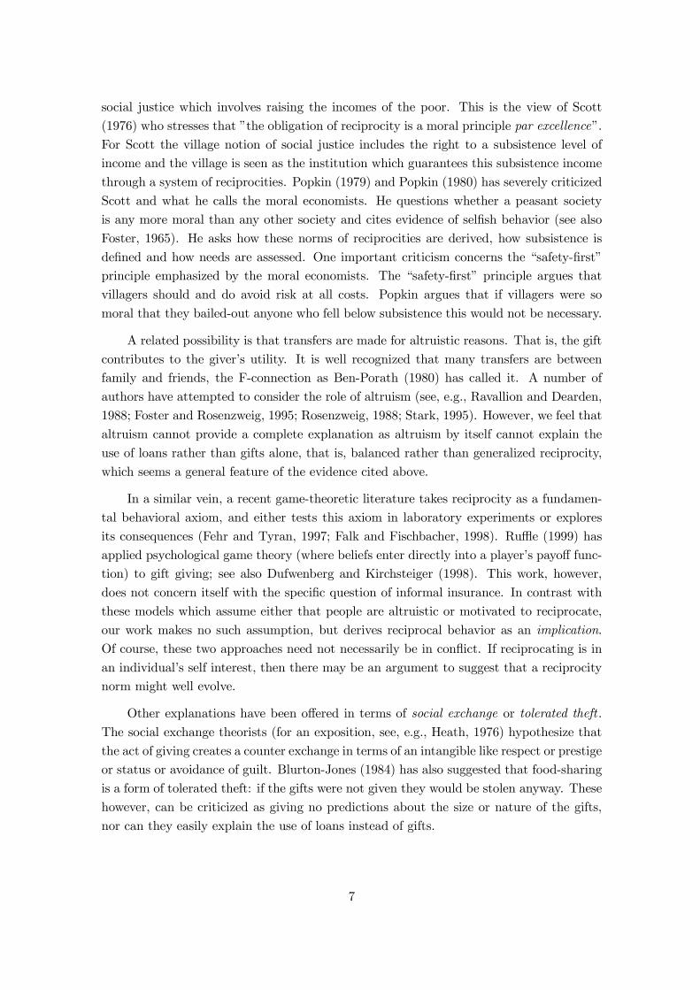
Figure 1: Relative Shares - Gifts Only

transfer and this helps risk-pooling which is to everyone’s bene…t. The cost of this is a

move away from an equal share when both receive 1000—extra variability is introduced—

but this cost is very small (formally, second-order) relative to the extra insurance when

one household’s income is 500 (which is …rst-order).

The above demonstrates that whenever the pure gift solution is unable to deliver

perfect insurance (i.e., whenever x < 250), there is a superior arrangement involving some

counter obligation. Moreover the argument just given does not depend on the speci…cs of

the income distribution (it generalizes to arbitrary …nite distributions). Exactly how the

loans and repayments are optimally arranged is discussed later but the optimal solution—

what we call the “dynamic limited commitment solution”— in the example with logarith-

mic utility and ±=20/21 and p = 0:1 is illustrated in Table 2. This solution is analysed

more explicitly in Ligon, Thomas, and Worrall (1997). It can be seen from the table that

the shares of income are less variable than in Table 1, so that more insurance is being

provided. It should be stressed that this is the best conceivable arrangement given the

constraint of voluntary participation, and in the remainder of the paper we shall investi-

gate the extent to which a simple implementation of counter obligation using interest-free

quasi credit measures up to this potentially complex ideal. Nevertheless, even in the best

arrangement, the element of counter obligation can be clearly seen. For example in period

421, household 1 makes a large insurance transfer to 2 who has received a low yield; in the

following two periods, yields return to parity, but 2 makes a small transfer to 1 (of 16.59).

It is the anticipation of this “repayment” which helps to persuade 1 to make such a large

initial transfer.

The variability in the shares indicate the extent of the insurance so it is worthwhile

11

considering a slightly more complicated example to illustrate how shares change over

time.16 A random sample of nine incomes was drawn from a lognormal distribution with

a mean and variance matching that in the data from the villages in rural India discussed

below. It was assumed that the two households have identical and independent income

draws, so there are a total of 81 states. The solutions were computed and income simulated

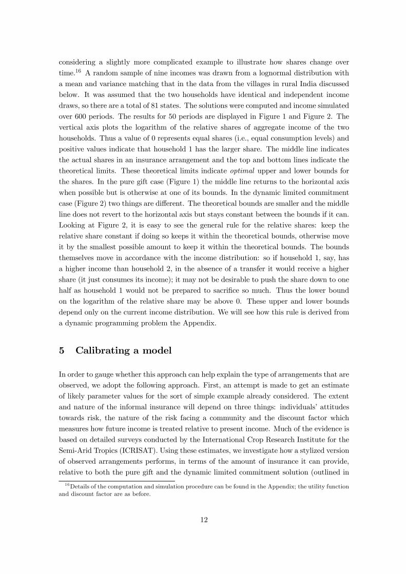
over 600 periods. The results for 50 periods are displayed in Figure 1 and Figure 2. The

vertical axis plots the logarithm of the relative shares of aggregate income of the two

households. Thus a value of 0 represents equal shares (i.e., equal consumption levels) and

positive values indicate that household 1 has the larger share. The middle line indicates

the actual shares in an insurance arrangement and the top and bottom lines indicate the

theoretical limits. These theoretical limits indicate optimal upper and lower bounds for

the shares. In the pure gift case (Figure 1) the middle line returns to the horizontal axis

when possible but is otherwise at one of its bounds. In the dynamic limited commitment

case (Figure 2) two things are di¤erent. The theoretical bounds are smaller and the middle

line does not revert to the horizontal axis but stays constant between the bounds if it can.

Looking at Figure 2, it is easy to see the general rule for the relative shares: keep the

relative share constant if doing so keeps it within the theoretical bounds, otherwise move

it by the smallest possible amount to keep it within the theoretical bounds. The bounds

themselves move in accordance with the income distribution: so if household 1, say, has

a higher income than household 2, in the absence of a transfer it would receive a higher

share (it just consumes its income); it may not be desirable to push the share down to one

half as household 1 would not be prepared to sacri…ce so much. Thus the lower bound

on the logarithm of the relative share may be above 0. These upper and lower bounds

depend only on the current income distribution. We will see how this rule is derived from

a dynamic programming problem the Appendix.

5 Calibrating a model

In order to gauge whether this approach can help explain the type of arrangements that are

observed, we adopt the following approach. First, an attempt is made to get an estimate

of likely parameter values for the sort of simple example already considered. The extent

and nature of the informal insurance will depend on three things: individuals’ attitudes

towards risk, the nature of the risk facing a community and the discount factor which

measures how future income is treated relative to present income. Much of the evidence is

based on detailed surveys conducted by the International Crop Research Institute for the

Semi-Arid Tropics (ICRISAT). Using these estimates, we investigate how a stylized version

of observed arrangements performs, in terms of the amount of insurance it can provide,

relative to both the pure gift and the dynamic limited commitment solution (outlined in

16Details of the computation and simulation procedure can be found in the Appendix; the utility functionand discount factor are as before.

12

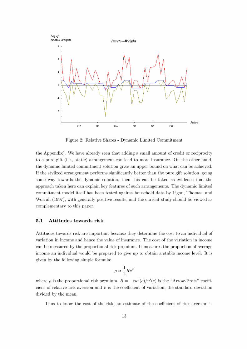
Figure 2: Relative Shares - Dynamic Limited Commitment

the Appendix). We have already seen that adding a small amount of credit or reciprocity

to a pure gift (i.e., static) arrangement can lead to more insurance. On the other hand,

the dynamic limited commitment solution gives an upper bound on what can be achieved.

If the stylized arrangement performs signi…cantly better than the pure gift solution, going

some way towards the dynamic solution, then this can be taken as evidence that the

approach taken here can explain key features of such arrangements. The dynamic limited

commitment model itself has been tested against household data by Ligon, Thomas, and

Worrall (1997), with generally positive results, and the current study should be viewed as

complementary to this paper.

5.1 Attitudes towards risk

Attitudes towards risk are important because they determine the cost to an individual of

variation in income and hence the value of insurance. The cost of the variation in income

can be measured by the proportional risk premium. It measures the proportion of average

income an individual would be prepared to give up to obtain a stable income level. It is

given by the following simple formula:

½ ¼ 1

2Rv2

where ½ is the proportional risk premium, R = ¡cu00(c)=u0(c) is the “Arrow-Pratt” coe¢-cient of relative risk aversion and v is the coe¢cient of variation, the standard deviation

divided by the mean.

Thus to know the cost of the risk, an estimate of the coe¢cient of risk aversion is

13

Choice Heads Tails Exp Value1 5 5 52 9.5 4.5 73 12 4 84 16 2 95 19 1 106 20 0 10

Table 3: Binswanger’s Experiment: The amounts are in Rs

needed. Binswanger (1980) and Binswanger (1981) conducted a series of experiments to

try to gauge risk aversion amongst the households in the ICRISAT survey. He o¤ered

a series of gambles where players were invited to choose one of the alternative gambles

outlined in Table 3. This was done repeatedly and with four di¤erent amounts of money

(in Rupees): the amounts in Table 3 were also divided by a factor of 10 and multiplied

by factors of 10 and 100. The …rst three of these games were played for real money; the

other game (where gamble 1 was a sure gain of 500Rs, etc.) was hypothetical. Someone

who consistently chooses gamble 1 is extremely risk averse and is prepared to give up a

large expected return for the safety of a certain gain. Someone who consistently chooses

gambles 5 or 6 is risk neutral and always goes for the highest expected returns no matter

what the risk. The modal choice was 3 or 4 indicating a moderate but not extreme risk

aversion. It corresponds to a coe¢cient of relative risk aversion of around 2. This means

that a household which faces a coe¢cient of variation of income is 0.4 and has a coe¢cient

of relative risk aversion of 2, would be prepared to pay 16% of its wealth in order to

stabilize its income.

Statistical evidence from Antle (1987) also seems to support these results and evidence

presented in Walker and Ryan (1990) also …nds that using the experimental results on risk

aversion helped explain actual choices of savings and investment in irrigation. That is, the

more risk averse players adopted more cautious strategies for investment decisions.

5.2 Risk

As already stated, risk is perhaps the most dominant factor of life in subsistence economies.

In the ICRISAT data the coe¢cient of variation of income ranged from 10% to 80% with

the majority falling in the 20% – 40% range. Thirty-two of the 108 households surveyed

in three of the ICRISAT villages Aurepalle, Kanzara and Shirapur, su¤ered one or more

years where income was 50% or more below the median income. In the Indian …shing

villages of Purakkad (mentioned above) and Poovar the coe¢cient of variation was even

higher at over 100% (Platteau, 1997).

As we have seen a household which faces a coe¢cient of variation of 0.4 and has a

coe¢cient of relative risk aversion of 2 is prepared to pay 16% of its wealth in order to

14

stabilize this income. The question is whether there is anyone in the village who would be

prepared to buy this risk. There are two possibilities: risk-sharing and risk-pooling.

A risk shared is a risk halved. Consider the following simple example with two

households both with a constant coe¢cient of relative risk aversion of 2. One has a risky

income of either 60 or 140 with equal probability (this gives an expected value of 100

and a coe¢cient of variation of 0.4). The other has a sure income of 100. Household 1

is prepared to pay 16 to eliminate its risk. Suppose however the two households share

their income 50:50 so each gets either 80 or 120 with equal probability. The coe¢cient of

variation is 0.2 for each so each would be prepared to pay 4 to eliminate the risk. The

total cost of the risk is now 8 rather than 16, so the cost of the risk has been halved. It is

also clear that there is a potential trade here. Household 1 would be prepared to pay 12

to reduce the variation from 0.4 to 0.2 and household 2 is willing to accept 4 to take on

the extra risk, i.e. increase its variation from 0 to 0.2. Thus a situation where household

2 accepts a premium of say 8 and agrees to share the risk 50:50 should be bene…cial to

both.

Of course there may be no one in the village who does not face risk so it is important

to know if it is still possible to trade risk when all face risks. This is known as risk

pooling. The extent to which this is possible depends on how covariate are the risks. For

example if household 2 also has an uncertain yield of 60 and 140 but when household 1

had 60 household 2 has 140 then the two risks are perfectly negatively correlated and by

sharing 50:50 they could perfectly stabilize their incomes. If on the other hand the risks

were perfectly positively correlated, then no sharing can reduce the risks. An informal

insurance arrangement can only work if incomes are not perfectly correlated. The degree

to which risks can be reduced will depend on the covariance or correlation between the

risks.

The evidence suggest that the covariances are, perhaps surprisingly, very low. The

covariances in the …shing villages of Poovar and Purakkad were very close to zero (see

Platteau (1997)). In the ICRISAT villages the correlations with average village income

were on average around 0.2 but varied from -0.7 to 0.9 (see Townsend (1994)). Thus there

seems to be great scope for risk-pooling. In our calibrated model, we shall assume that

the covariances are zero.

5.3 The discount rate

The rate at which villagers discount the future is also important. If they completely

discounted the future (± = 0), then there would be no reason to make gifts or loans as the

future reciprocation would not be valued. At the other extreme, if they were very patient

(± ¼ 1); then the best (pure gift) arrangement would be sustainable as any short-run costfrom sacri…cing current resources would always be outweighed by the long-term bene…ts

15

Choice September 1990 September 1991 Implied Discount Rate1 10 Kg 9 Kg -10%2 10 Kg 10 Kg 0%3 10 Kg 11 Kg 10%4 10 Kg 12 Kg 20%5 10 Kg 13 Kg 30%6 10 Kg 15 Kg 50%7 10 Kg 17 Kg 70%8 10 Kg 20 Kg 100%

Table 4: Pender’s Experiment

of insurance.

Pender (1996) conducted a series of experiments to …nd out the discount rate amongst

villagers in Aurepalle (one of the ICRISAT villages). Like the experiments of Binswanger,

these were real rather than hypothetical experiments. Respondents were asked to state

their preference over a series of choices between quantities of rice and the date they would

be received like those in Table 4. The rightmost column shows the implied discount

rate if the respondent was indi¤erent between the two alternatives. Thus if a respondent

picked September 1990 (now) in choices 1–4 but September 1991 in choices 5–8, then the

discount rate would be in the range 20%–30%. Each respondent answered three similar

sets of choices with di¤erent base amounts and then one choice was randomly assigned as

a reward. Thus if the respondent chose September 1991 in choice 8 in Table 4 and this

was the choice assigned to him, then he would receive 20 Kg of rice in September 1991.

There were two key features of the results. The discount rates were highly variable and

the average rate was extremely high compared to the results from similar experiments

conducted in industrialized societies. The median discount rate was above 50% implying

that most respondents would prefer to have 10 Kg now rather than 15 Kg in one years

time.

It is important to note that these experiments are designed to …nd the intertemporal

marginal rate of substitution. That is how one person values consumption now against

consumption in the future. In fact the discount rate that is needed for calibrating the

model is the rate of pure time preference: that is, how a person values extra utility now

against extra utility in the future, or equivalently how a person values extra consumption

now against extra consumption in the future with consumption the same in both periods.

If, however, average consumption is approximately constant and if marginal utility is a

convex function of income (u000(c) ¸ 0; which is true of the logarithmic utility function),then Pender’s estimates provide a lower bound for the rate of pure time preference. This

implies an upper bound for the discount factor, which is one over one plus the rate of pure

time preference, of about two-thirds.

16

6 Gifts and Loans

In this section we ask whether a scheme of gifts and loans can come close to achieving what

can be achieved by the dynamic limited commitment solution. We use estimates for the

discount factor, coe¢cient of variation and coe¢cient of risk aversion in the range discussed

in the previous section. This is vital for the theory which we are proposing: for some

parameter values the theory gives trivial answers. For example, holding the coe¢cient

of variation and coe¢cient of risk aversion constant, if households are very impatient (±

near zero), putting little weight on the future, it turns out that no risk-pooling is possible

because the (heavily discounted) future gains from insurance will never outweigh the loss

from sacri…cing current resources today. Similarly, if they are very patient (± near 1)

the future gains will always be so large relative to current losses that perfect insurance is

possible, and consequently gifts alone are used in the gift/loan arrangement (which is then

identical to the dynamic limited commitment solution), and there would be no balanced

reciprocity.

The model is a general version of the example outlined in Section 4. There are two

identical households who have an income of y and a probability p of a loss of size d. The

risks are independent and hence the coe¢cient of variation is

v =

p(p(y ¡ d¡m)2 + (1¡ p)(y ¡m)2)

m

where m = p(y ¡ d) + (1¡ p)y is average income. The gift/loan scheme we consider is asfollows. When one household su¤ers a loss, the other gives it a gift of G and makes an

interest-free loan of L. As we have seen in section 4 the addition of an interest-free loan can

lead to improvements in risk sharing. Next period, if neither su¤ers a loss then the loan

L is repaid. If the same household receives a loss the gift and loan are repeated (i.e., in

this case the loan is written o¤). If both households su¤er a loss then the loan repayment

is reduced to L0 in such a way that the loan repayment is reduced proportionally to thereduction in income (so that the loan is e¤ectively written down; in the example of section

4 the write-down was 100).

L0 = (y ¡ dy)L:

If the other household su¤ers a loss then he receives the gift of G and loan of L and the

previous loan is forgotten. This scheme has the virtue of being very simple and accords

well with the evidence presented above that gifts and interest-free loans are both used and

that sometimes loans are forgiven if circumstances dictate.

To see how this scheme works, consider the case where there are no loans outstanding.

There are four possible situations. Both su¤er no loss, which we label nn; both su¤er a loss,

which we label ll; or one su¤ers a loss and the other does not, which are labelled nl and ln.

Let V denote the surplus over autarky (i.e., the di¤erence between expected discounted

utility under the scheme and under autarky) before the yields are known and let Vnn

17

denote the surplus when neither su¤ers a loss, Vnl denote the surplus of a household when

only the other household su¤ers a loss, etc., assuming that there are no loans outstanding

from the previous period. Then

V = (1¡ p)2Vnn + p2Vll + p(1¡ p)Vnl + (1¡ p)pVln:

Since no payments are made in the situations where neither or both su¤er a loss, then

next period we start again from the same position of no outstanding loans. Thus

Vnn = ±V

and

Vll = ±V:

If the second household su¤ers a loss, then he receives a gift of G and loan of L and so

the surplus for the …rst household is

Vnl = u(y ¡G¡ L)¡ u(y)+ ±(1¡ p)2(u(y + L)¡ u(y) + ±V )+ ±p2(u(y ¡ d+ L0)¡ u(y ¡ d) + ±V )+ ±p(1¡ p)Vnl + ±(1¡ p)pVln:

The …rst line is the loss in utility of givingG and loaning L; the second line is the discounted

gain if neither su¤ers a loss so L is repaid and we start again from the situation of no

outstanding loan; the third line is likewise the discounted gain from the loan repayment of

L0 if both su¤er a loss and starting again from no outstanding loan; and the last line is thediscounted surplus in states nl and ln, where Vln is calculated similarly by the equation

Vln = u(y ¡ d+G+ L)¡ u(y ¡ d)+ ±(1¡ p)2(u(y ¡ L)¡ u(y) + ±V )+ ±p2(u(y ¡ d¡ L0)¡ u(y ¡ d) + ±V )+ ±p(1¡ p)Vnl + ±(1¡ p)pVln:

It is possible to solve explicitly for V , Vnl and Vln using these equations to give:

V =®(Y + Z)

1¡ 2±®Vnl = Y + ±V =

(1¡ ±®)Y + ±®Z1¡ 2±®

Vln = Z + ±V =±®Y + (1¡ ±®)Z

1¡ 2±®where

® =p(1¡ p)

1¡ ±(1¡ 2p(1¡ p))

18

Y = u(y ¡G¡ L)¡ u(y)+±(1¡ p)2(u(y + L)¡ u(y)) + ±p2(u(y ¡ d+ L0)¡ u(y ¡ d))

Z = u(y ¡ d+G+ L)¡ u(y ¡ d)+±(1¡ p)2(u(y ¡ L)¡ u(y)) + ±p2(u(y ¡ d¡ L0)¡ u(y ¡ d)):

The objective is to choose G and L so as to maximize V . However, the household must

always have an incentive to provide the gift and loan, so

Vnl = Y + ±V ¸ 0 (1)

and must have an incentive to repay the loan17

u(y ¡L)¡ u(y) + ±V ¸ 0: (2)

Given the estimates of Section 5, we choose y = 100 (for illustrative purposes; none of

the comparisons depend on the level) and take as a base case the following values for

the parameters: coe¢cient of variation v = 0:45 and the discount factor ± = 0:65; the

coe¢cient of relative risk aversion is R = 2 and we use the constant relative risk-aversion

utility function u(c) = c1¡R=(1 ¡ R) (or log c for R = 1). These parameter values are

…rmly in the middle of the ranges given in the last section.18 With a coe¢cient of variation

v = 0:45 and a probability of loss p = 0:5 the implied loss is d =$62:07.19 While it is

not possible to obtain an analytical solution for the optimum gift and loan, it is possible

to do so numerically. It is clear that either (1) or (2) holds as an equality unless perfect

insurance is possible. Thus by gridding over 100 values for L and choosing the values of

G which satisfy the constraints, it is then possible to …nd the combination of G and L

which attains the highest value for V and simultaneously satisfy both constraints. The

optimum is G =$21:01 and L =$5:90.20 Thus when one household su¤ers a loss its income

is y¡d+G+L =$64:84 and the other’s net income is y¡G¡L =$73:09. The repaymentnext period is either $5:90 if neither su¤ers a loss and $2:24 if both su¤er a loss.

As a contrast we consider a situation of generalized reciprocity where only gifts are

used and a system of pure credit where only interest-free loans are used. In the system of

generalized reciprocity, the optimal gift is $24:87 and in the case of pure credit, the optimal

loan is $1:06 with a repayment of $0:41 if both households su¤er a loss. We see that gifts

alone do quite well but gifts and loans together provide a distinct improvement. Loans by

themselves prove to be inadequate. The reason is that the loan payment improves risk-

sharing but the loan repayment harms risk-sharing. The purpose of the loan repayment is

17For R > 1, u(y¡L)¡u(y) > u(y¡ d¡L0)¡u(y¡ d) as u(y¡L)¡u(y)¡ (u(y¡ d¡L0)¡u(y¡ d)) =((1¡ (L=y))(1¡R) ¡ 1)(y(1¡R) ¡ (y ¡ d)(1¡R))=(1¡R) ¸ 0.18We have presumed that the covariance is zero.19A value for the coe¢cient of variation and for y does not …x the distribution even if it is assumed to

be two point, as here. Nevertheless simulations suggest that our result are not particularly sensitive to theway that this is broken up into p and d.20A Mathematica package is available from the authors.

19

to encourage risk-sharing when incomes are di¤erent. But with loans alone, this is di¢cult

and the loan cannot be raised much without running into the constraint (2). The reason

that a higher value for L is possible in the combined gift/loan scheme is that the gift

element allows much more insurance, so that higher loan repayments are sustainable due

to the fact that there is more to lose, in terms of future insurance, if a repayment is not

made.

A better comparison can be made by calculating the surpluses—the increase in utility

over autarky—from each scheme. We do this relative to the most e¢cient (i.e., the dynamic

limited commitment) scheme. The most e¢cient scheme involves more complicated gifts

and loans and repayments over more than one period. The procedure for calculating

the e¢cient contract is outlined in the Appendix. The purpose here is to show that a

simple system of gifts and loans can do extremely well and do almost as well as the more

complicated contract. The gift/loan scheme achieves 99:62% of the total possible surplus

from the most e¢cient scheme. The generalized reciprocity scheme of gifts scores 98:40%

and the pure credit scheme of loans only scores 8:37%. Thus some loan element is bene…cial

when combined with gifts, although for these parameter values only mildly so. In the next

section it is shown that for parameter values close to these ones, the loan element can be

much more valuable.

7 Sensitivity

In this section we examine how sensitive the estimates are to the parameter values. We …rst

consider how gifts and loans in the combined gift/loan arrangement respond to di¤erent

parameter values around the base case given in Section 6 with income in the no loss state

y = 100, the coe¢cient of risk aversion R = 2, the discount factor ± = 0:65 and the

coe¢cient of variation v = 0:45. This is shown in Figure 7 for the three parameters; the

coe¢cient of risk aversion; the discount factor and the coe¢cient of variation. We take

the parameters to range within the values suggested in Section 5.

Thus the …rst panel shows values for the coe¢cient of risk aversion between 1 and 2.5

with the discount factor …xed at ± = 0:65 and the coe¢cient of variation …xed at v = 0:45.

As risk aversion increases, the (future) bene…ts from mutual insurance rise (relative to the

current cost of making a transfer to the other party), and this allows more insurance to

be provided. Thus, for a value of risk aversion close to one, no gift/loan combination is

sustainable; for slightly higher values of risk aversion, some insurance is possible and loans

are more important than gifts. Eventually as the coe¢cient of risk aversion increases,

gifts dominate loans, and for a value of the coe¢cient of risk aversion above 2.35 complete

insurance is possible and so no loan element is required. A similar picture obtains as the

other two parameter values are varied. The second panel shows how the gifts and loans

vary as the discount factor varies between 0.36 and 0.72 with the other parameters …xed at

20

Figure 3: Gifts and Loans

their baseline values. At a discount factor of below 0.38, no insurance is possible and for a

discount factor above 0.72, complete insurance is possible. In between, gifts increase and

loans increase at …rst but become less important for higher discount factors. A similar

pattern emerges from the third panel which plots gifts and loans as the coe¢cient of

variation ranges between 0.1 and 0.8. For values of v above 0.55, full insurance is possible

and for values below 0.2, no insurance is possible. At low values of v, both gifts and loans

increase as v rises but eventually loans become less important.21The next …gure, Figure

4, plots the surpluses relative to the dynamic limited commitment surplus for the same

range of parameter values. The solid line is the percentage surplus from gifts and loans;

the dotted line from gifts alone and the dashed line from loans alone. It shows how well

each of these arrangements does. Since these surpluses are relative to the dynamic limited

commitment surplus, a value of 100% is the theoretical maximum for all parameter values.

As can be seen gifts easily dominates loans and gifts and loans together dominate either

(as we know from the result in Section 4). From the …rst panel it can be seen that for a low

value of the coe¢cient of risk aversion such as R = 1:1, the gift only arrangement attains

3% of the most possible whereas gifts and loans together achieve 91%. This dominance

is preserved although diminished as R rises until it is possible to obtain complete risk

sharing with gifts alone for R > 2:35. The second and third panels show a similar story as± and v are varied. From each case it appears that the combination of gifts and loans can

do considerably better than gifts alone provided that some but not complete insurance is

possible.

21Gifts continue to rise for v > 0:55 as the loss of income in the bad state increases with v.

21

Figure 4: Relative Surpluses

8 Conclusion

A key feature of the informal insurance arrangements in rural communities discussed in

the introduction is the use of gifts and informal loans which are uncollateralized and pay

no interest. There is a presumption that gifts will be reciprocated and loans repaid unless

adverse circumstances dictate otherwise. That is, mutual insurance takes the form of

balanced reciprocity or quasi-credit.

We have shown that quasi-credit arrangements can be the outcome of a dynamic

game when reciprocation is the voluntary action of rational agents rather than enforced.

If reciprocation were obligatory, gift-giving alone as need arises would be the best arrange-

ment. Quasi-credit is less e¤ective as if a household borrows in the face of an adverse shock

and then immediately su¤ers another adverse shock, it has repayment obligations on the

borrowing already made, and unless it is willing to accumulate even more debt, it will

be forced to cut consumption. Had it received a gift without counter obligation after the

…rst shock, it would be in no worse position after the second shock, and provided another

gift is made, it would be able to maintain its consumption. The problem with a pure gift

arrangement in this case is that the counter obligation may not be su¢cient to induce

the giver to part with resources today. On the other hand, if there is a credit element to

the transaction, the giver will expect some future reward—repayment on the loan—over

and above any reciprocal insurance promise, and this may provide su¢cient incentive to

induce the giver to part with resources today.

The exact nature of the quasi-credit arrangement depends upon a few key parameters.

22

These are the size of the risk as measured by the coe¢cient of variation and the covariance

of household incomes; the degree to which households are a¤ected by risk as measured by

the coe¢cient of risk aversion; and the rate at which households discount future as mea-

sured by the rate of pure time preference. The ICRISAT data on villages in southern India

allows estimates for these parameters and we have calibrated the model using estimates

from this literature. Using this calibration, we are able compute the best quasi-credit ar-

rangements for some simple examples. In addition we are able to compare the outcome to

the optimum dynamic limited commitment outcomes which are discussed in the Appendix.

The latter arrangements are more complex because the loan repayments are spread over

many periods and depend upon the sequence of shocks. Nevertheless it is shown that for

a range of typical parameter values a very simple quasi-credit scheme does almost as well

as the more complex dynamic limited commitment arrangement. This suggest that the

advantage of the dynamic element can be adequately captured by a simple interest-free

loan element and that the quasi-credit arrangements used in practice are very close to op-

timum when reciprocity is voluntary. Thus not only is balanced reciprocity a theoretical

possibility in the model, for plausible parameter values, it can achieve something close the

best insurance that can be attained.

Is the approach to reciprocity outlined in this paper applicable outside of the contextof mutual insurance in rural communities? In principle, it is relevant to any situation inwhich risk is important and the need for informal insurance arises. An obvious example iswithin-family transfers even in economies where developed insurance markets, private orpublic, exist. Such markets su¤er from a number of imperfections, especially because of thedi¢culties and cost of obtaining all relevant information, and thus there is a bene…t to behad from insurance arrangements in the context where information ‡ows more freely (thefamily) although participation cannot be enforced through legal means. Even outside ofan insurance context the analysis is potentially applicable, for example in any continuingrelation where each party can undertake costly actions, which may or may not involvemonetary transfers, that have a bene…t to the other party. Whenever these bene…ts‡uctuate over time, either randomly or deterministically,22 so that party A today bene…tsfrom an action taken by party B and there is a likelihood in the future that party Bwill bene…t from an action taken by party A at that time, then the principle of balancedreciprocity can be used to help sustain higher levels of mutual cooperation.

9 Appendix

The Appendix outlines a general model with H households and shows how the optimumrisk-pooling arrangement under dynamic limited commitment can be derived and solutionnumerically computed. It provides an upper bound to how well a simple arrangement ofgifts and loans can do. This problem is similar in structure to that analyzed by Thomasand Worrall (1988), and we borrow heavily from that analysis and from Hayashi (1996).

Each period t = 1; 2; ::: , household i (i = 1; 2; : : : ; H) receives an income yi(s) > 0

22The model developed in the Appendix is general enough to cover deterministic ‡uctuations.

23

of a single perishable good, where s is the state of nature drawn from a …nite set s 2 S,and S = f1; 2; :::; Sg. The state is a su¢cient statistic for the income distribution at anyparticular date. It is assumed that the state of nature follows a Markov process with theprobability of transition from state s to state r given by ¼sr. This formalization includes asa special case an identical and independent distribution over the possible states of nature(¼sr is independent of s). The general speci…cation of the dependence of incomes yi(s) onthe state of nature allows for arbitrary correlation between the two incomes, although in thesimulations we have assumed that incomes are independently and identically distributed.

Household i has a per-period (“von-Neumann-Morgernstern”) utility of consump-tion function ui(ci) which displays positive but diminishing marginal utility: u0i(ci) > 0;u00i (ci) < 0: Households are in…nitely lived, discount the future with common discountfactor ±, and are expected utility maximizers. We assume that at date 0; before any un-certainty is resolved, the households enter into an implicit risk-sharing arrangement. Afteran arrangement violation by any party (failure to make a transfer to another householdwhen one is supposed to), all households consume at autarky levels (i.e., consume theirown income) thereafter.

What we refer to below as sustainable arrangements can be shown to correspondprecisely to the non-cooperative subgame-perfect equilibrium outcomes of the dynamicgame; since reversion to autarky is the most severe subgame-perfect punishment, not onlydoes a sustainable arrangement correspond to a subgame-perfect equilibrium outcome, butalso there can be no other equilibrium outcomes other than those characterized by usingreversion to autarky as a punishment.23

Let st be the state of the world occurring at date t. An arrangement will specify forevery date t and for each history of states up to and including date t, ht = (s1; s2; :::; st),a consumption level ci(ht). De…ne U i(ht) to be the expected discounted utility gain overautarky or surplus of household i from the arrangement from period t onwards, discountedto period t, if history ht = (ht¡1; st) occurs up to period t:

U i(ht) = (1¡ ±)(ui(ci(ht))¡ ui(yi(st))) +E1X

j=t+1

(1¡ ±)±j¡t(ui(ci(hj))¡ ui(yi(sj)));

where E denotes expectation, conditional on ht; and per-period utility has been normalizedby multiplying by (1 ¡ ±). The …rst term in the above equation is the short run gainfrom the arrangement and the second term is the long-run or continuation gain from thearrangement. This equation can be de…ned recursively as

U i(ht) = (1¡ ±)(ui(ci(ht))¡ ui(yi(st))) + ±SXr=1

¼srUi(ht; r):

Household i will have no incentive to break the arrangement if the following sustainabilityconstraint holds at each date t after every history ht:

U i(ht) ¸ 0:If these equations hold for all i = 1; : : : ;H, then we call the arrangement sustainable.23The argument is simply that any equilibrium outcome supported by a less severe credible punishment,

can also be supported by the more severe punishment considered here.

24

A sustainable arrangement is e¢cient if there is no other sustainable arrangementwhich Pareto dominates it. In the space of discounted utilities, the Pareto frontier is setof utilities corresponding to e¢cient arrangements. The Pareto frontier at any date t andgiven the current state s depends only on s and not on the past history which led to thisstate. This allows us to simplify and abuse notation slightly by letting U ir denote thecontinuation utility of household i when the state is r. Also let the Pareto frontier in stater be de…ned implicitly by the function Tr(U1r ; : : : ; U

Hr ) = 0. Similar arguments to those

given in Thomas and Worrall (1988) show that the set de…ned by 0 ¸ Tr(U1r ; : : : ; UHr ) isa convex set (i.e., all points lying on a straight line between any two points in the set alsolie in the set).

To …nd the Pareto-e¢cient arrangement, …rst consider the following maximizationproblem.

max(cis)

Hi=1;((U

ir)Sr=1)

Hi=1

HXi=1

wif(1¡ ±)(ui(cis)¡ ui(yis)) + ±SXr=1

¼srUirg

subject to

0 ¸ Tr(U1r ; : : : ; U

Hr ) 8r 2 S

U ir ¸ 0; 8r 2 S 8i = 1; : : : ; HHXi=1

cis = Ys

cis ¸ 0 8i = 1; : : : ;H

where wi is the “Pareto-weight” and Ys =PHi=1 y

is is aggregate income in state s. Following

Hayashi (1996) this problem can be decomposed into a number of sub-problems. The …rstsub-problem is the e¢cient consumption at any date for a given set of Pareto-weights.

max(ci)Hi=1

HXi=1

wiui(cis) s:t:

HXi=1

cis = Ys and cis ¸ 0 8i = 1; : : : ;H:

The …rst-order conditions are for any pair of households i and k

u0i(cis)u0k(cks)

=wkwi+Ãk ¡ Ãiwiu0k(cks)

where Ãi is the “Lagrange” multiplier on the non-negativity constraint for household iconsumption. We can write the solution as ci(w;Ys) where w = (w1; : : : ; wH) is the vectorof Pareto-weights and an “indirect utility function” as vi(w;Ys) = ui(ci(w; Ys)).

There are also S sub-problems of the form

max(U ir)

Hi=1

HXi=1

wiUir s:t: 0 ¸ Tr(U1r ; : : : ; UHr ) and U ir ¸ 0 i = 1; : : : ;H:

The …rst-order conditions give for any pair of households i and k

wk + Ákr

wi + Áir

=@Tr=@U

kr

@Tr=@U ir;

25

where Áir is the multiplier on the sustainability constraint for household i. It is clearas argued above that the solution involves Tr(U1r ; : : : ; U

Hr ) = 0, so that the continuation

arrangement is itself e¢cient. Consider then the Pareto problem without the sustainabilityconstraints where the weights are denoted ~w to distinguish it from the former problem:

max(U ir)

Hi=1

HXi=1

~wiUir s:t: 0 ¸ Tr(U1r ; : : : ; UHr ):

The …rst-order conditions give~wk~wi=@Tr=@U

kr

@Tr=@U ir:

Denote the solution V i( ~w; r) = U ir( ~w) for each household i, as the conditional householdvalue function (conditional on the state). These value functions map Pareto-weights tocontinuation utilities in a Pareto-e¢cient way. They obey the simple recursive relationship

V i(w; s) = (1¡ ±)(vi(w; Ys)¡ ui(yis)) + ±SXs=1

¼srVi( ~w; r):

Then the S sub-problems can be replaced by

max( ~wi)Hi=1

HXi=1

wiVi( ~w; r) s:t: V i( ~w; r) ¸ U ir 8i = 1; : : : ;H;

where the value functions are used so that the next period Pareto-weights ~w become themaximand instead of the continuation utilities. It is clear from di¤erentiating the …rst-order conditions for this problem that

HXi=1

~wi@V i( ~w; r)

@ ~wk= 0 8k = 1; : : : ; H;

so that in the absence of the sustainability constraint, the solution is ~w = w and thePareto-weights change only in response to binding sustainability constraints.

The relationship between ~w and w when there are binding sustainability constraintscan be described by combining the …rst-order conditions for the two problems de…nedabove:

~wk~wi=wk=wi + Á

kr=wi

1 + Áir=wi:

This gives an updating rule for the ratio of the Pareto-weights. Thus given an initialset of weights the arrangement can be computed recursively by updating the weights asdetermined by the actual state and the equation given above.

To solve the above problem it is necessary to determine the conditional value functionsV i(w; r). These can be calculated using an iterative procedure starting with the …rst-bestvalue functions (where the sustainability constraints are ignored). We will outline thisprocedure for the case considered in the main text, of two households where the statesare identically and independently distributed over time (¼sr = ¼r). It is computationallysimpler to work with the unconditional value functions

W i(w) =SXr=1

¼rVi(w; r):

26

In the i.i.d. case with two households there are just two unconditional value functions,one for each household.24 The Pareto-weights can be normalized so

PHi=1wi = 1, so with

two households it is only necessary to calculate one weight. To distinguish this case, let µbe the Pareto-weight for household 1 and let 1¡ µ be the Pareto-weight for household 2.

There is then a simple procedure for calculating the two unconditional value func-tions, W i(µ). First calculate the indirect utility functions vi(µ; Ys) and compute an initialunconditional …rst-best value function as follows:

W i0(µ) =

SXs=1

¼s(vi(µ; Ys)¡ ui(yis)):

Next compute U is and solve the 2S equations

(1¡ ±)(vi(µ; Ys)¡ ui(yis)) + ±W i0(µ) = U

is

for µ. This gives S intervals [µs; ¹µs] where µs is computed from the equations for household1 and ¹µs is computed from the equations for household 2. These intervals correspond tothe theoretical bounds drawn in the …gures in Section 4. New values of µ; say ~µ; can becomputed by the rule that µ is kept constant if it falls within the interval or moves to thenearest endpoint if it does not. 25 This gives ~µ as a function of µ in state s, say ~µs(µ).Two new value functions can then be computed according to

W i1(µ) =

SXs=1

¼s((1¡ ±)(vi(~µs(µ); Ys)¡ ui(yis)) + ±W i0(~µs(µ)))

and the process repeated until the di¤erence between the value functions W ij+1(µ) and

W ij (µ) or the di¤erence between the interval endpoints [µs; ¹µs] at successive iterations is

arbitrarily small.26 This computation procedure and the simulation of predicted consump-tions can be implemented with a Mathematica package.27

24 In general there are HS value functions to compute.25For a proof see Ligon, Thomas, and Worrall (1997).26 It can be shown that starting with the …rst-best value functions as described above, convergence is

assured.27The package is available upon request. The package solves the two identical household problem with

constant relative risk aversion. It computes the solution to the perfect insurance, pure gift and dynamiclimited commitment problems and simulates predicted consumptions for each model.

27

References

Antle, J. (1987): “Econometric Estimation of Producers’ Risk Attitudes,” AmericanJournal of Agricultural Economics, 69(3), 509–522.

Bardhan, P. (ed.) (1989): The economic theory of agrarian institutions. Oxford Uni-versity Press.

Ben-Porath, Y. (1980): “The F–Connenction: Families, Friends and …rms and theorganisation of exchange,” Population and Development Review, 6(1), 1–30.

Besley, T., S. Coate, and G. Loury (1993): “The Economics of Rotating Savings andCredit Associations,” American Economic Review, 83(4), 792–810.

Binswanger, H. (1980): “Attitudes toward Risk: Experimental Evidence from RuralIndia,” American Journal of Agricultural Economics, 62(3), 395–407.

(1981): “Attitudes toward risk: Theorectical implications of an experiment inrural India,” Economic Journal, 91, 867–890.

Bliss, C., and N. Stern (1982): Palanpur: The Economy of an Indian Village. OxfordUniversity Press.

Blurton-Jones, N. (1984): “A sel…sh origin for human food sharing: Tolerated Theft,”Ethology and Sociobiology, 5, 1–3.

Braverman, A., and J. Guasch (1986): “Rural credit markets and institutions indeveloping countries: Lessons for policy analysis from practice and modern theory,”World Development, 14(10/11), 1253–1267.

Camerer, C. (1988): “Gifts as economic signals and social symbols,” American Journalof Sociology, 94, supplement, S180–S214.

Cashdan, E. (1985): “Coping with Risk: Reciprocity among the Basarwa of NorthernBotswana,” Man, 20, 454–474.

(ed.) (1990): Risk and uncertainty in tribal and peasant economies. WestviewPress.

Coate, S., and M. Ravallion (1993): “Reciprocity without Commitment: Character-isation an Performance of Informal Insurance Arrangements,” Journal of DevelopmentEconomics, 40, 957–976.

Dufwenberg, M., and G. Kirchsteiger (1998): “A theory of sequential reciprocity,”CentER Discussion Paper No. 9837, Tilburg University.

Eswaren, E., and A. Kotwal (1989): “Credit as Insurance in Agrarian Economies,”Journal of Development Economics, 31, 37–53.

Fafchamps, M. (1992): “Solidarity Networks in Preindustrial Societies: Rational Peas-ants with a Moral Economy,” Economic Development and Cultural Change, 41(1), 147–174.

Falk, A., and U. Fischbacher (1998): “A theory of reciprocity,” Unpublishedmanuscript, University of Zurich.

Fehr, E., and J.-R. Tyran (1997): “Institutions and Reciprocal Fairness,” NordicJournal of Political Economy, 23, 133–144.

28

Firth, R., and B. Yamey (eds.) (1964): Capital, Saving and Credit in Peasant Soci-eties: Studies from Asia, Oceania, the Caribbean and middle America. George Allenand Unwin.

Foster, A., and M. Rosenzweig (1995): “Imperfect Commitment, Altruism and theFamily: Evidence from Transfer Behaviour in Low-Income Rural Areas,” Unpublishedmanuscript, University of Pennsylvania.

Foster, G. (1965): “Peasant Society and the Image of Limited Good,” American An-thropologist, 67, 293–315.

Goerlich, J. (1996-97): “Ceremonial gift exchange and barter in Melanesia: A gametheoretical di¤erentiation,” Angewandte Sozialforschung, 1-2, 37–46.

Gordon, B. (1975): Economic Analysis before Adam Smith: Hesiod to Lessius. MacMil-lan.

Gouldner, A. (1960): “The norm of reciprocity: A preliminary statement,” AmericanSociological Review, 25, 161–178.

Granovetter, M. (1985): “Economic Action and Social Structure: The Problem ofEmbededness,” American Journal of Sociology, 91, 481–510.

Hayashi, F. (1996): “Anaylsis of Household Savings: Past, Present and Future,” TheJapanese Economic Review, 47(1), 21–33.

Heath, A. (1976): Rational Choice and Social Exchange: A Critique of Exchange Theory.Cambridge University Press.

Hoff, K., A. Braverman, and J. Stiglitz (eds.) (1994): The Economics of RuralOrganisation: Theory, Practice and Policy. Oxford University Press.

Kimball, M. (1988): “Farmers’ Cooperatives as Behaviour towards Risk,” AmericanEconomic Review, 78, 224–236.

Ligon, E., J. P. Thomas, and T. Worrall (1997): “Informal Insurance Arrangementsin Village Economies,” Review of Economic Studies, forthcoming.

Lipton, M. (1968): “The Theory of the Optimising Peasant,” Journal of DevelopmentStudies, 4, 327–351.

Lund, S., and M. Fafchamps (1997): “Risk-Sharing Networks in Rural Philippines,”Unpublished manuscript, Stanford University.

Malinowski, B. (1978): Argonauts of the western Paci…c. Routledge.

Mauss, M. (1990): The gift: The form and reason for exchange in archaic societies.Routledge.

Millet, P. (1984): “Hesiod and his World,” BOOK of the Cambridge Philological Society,30, 94–115.

Nettle, D., and R. Dunbar (1997): “Social Markers and the Evolution of ReciprocalExchange,” Current Anthropology, 38(1), 93–99.

Pender, J. (1996): “Discount Rates and Credit Markets: Theory and Evidence fromRural India,” Journal of Development Economics, 50(2), 257–296.

29

Platteau, J, P. (1991): “Traditional systems of social security and hunger insurance:Past achievements and modern challenges,” in Social Security in Developing Countries,ed. by E. Ahmad, J. Dreze, J. Hils, and A. Sen. Clarendon Press.

(1997): “Mutual Insurance as an Elusive Concept in Traditional Rural Societies,”Journal of Development Studies, 33(6), 764–796.

Platteau, J, P., and A. Abraham (1987): “An Inquiry into Quasi-Credit Contracts:The Role of Reciprocal Credit and Interlinked Deals in Small-Scale Fishing Communi-ties,” Journal of Development Studies, 23(4), 461–490.

Popkin, S. (1979): The Rational Peasant. Univesrity of California Press.

(1980): “The Rational Peasant: The Political Economy of Peasant Society,”Theory and Society, 9, 411–471.

Posner, R. (1980): “A theory of primitive society, with special reference to law,” Journalof Law and Economics, 23, 1–53.

(1981): The economics of justice. Harvard University Press.

Raub, W., and J. Weesie (1990): “Reputation and E¢ciency in Social Interactions: AnExample of Network e¤ects,” American Journal of Sociology, 96(3), 626–654.

Ravallion, M., and L. Dearden (1988): “Social security in a "moral economy": Anempirical analysis for Java,” Review of Economics and Statistics, 70, 36–44.

Rosenzweig, M. (1988): “Risk, implicit contracts and the family in rural areas of low–income countries,” Economic Journal, 98, 1148–1170.

Ruffle, B. J. (1999): “Gift giving with emotions,” Journal of Economic Behavior andOrganization, 39, 399–420.

Sahlins, M. (1974): Stone Age Economics. Tavistock, London.

Schwatz, B. (1967): “The Social Psychology of the Gift,” American Journal of Sociology,73, 1–11.

Scott, J. (1976): The Moral Economy of the Peasant. Yale University Press.

Stark, O. (1995): Altruism and beyond: An economic analysis of transfers and exchangeswithin families and groups. Cambridge University Press.

Telser, L. (1980): “A theory of self-enforcing agreements,” Journal of Business, 53,27–44.

Thomas, J. P., and T. Worrall (1988): “Self-Enforcing Wage Contracts,” Review ofEconomic Studies, 55(4), 541–554.

Townsend, R. (1993): The Medieval Village Economy: A Study of the Pareto Mappingin General Equilibrium Models. Princeton University Press.

(1994): “Risk and Insurance in Village India,” Econometrica, 62(3), 539–591.

(1996): “Micro enterprise and Macro policy,” Paper presented at 7th worldcongress of the Econometric Society, Tokyo.

Udry, C. (1994): “Risk and Insurance in a Rural Credit Market: An Empirical Investi-gation in Northern Nigeria,” Review of Economic Studies, 63, 495–562.

Walker, T., and J. Ryan (1990): Village and Household Economies in India’s Semi-aridTropics. John Hopkins.

30