RECIPROCITY AND EMC MEASUREMENTS

Jasper J. Goedbloed Philips Research, Eindhoven, The Netherlands

(jjg@iae.nl) Abstract: Reciprocity theorems for electrical networks and electromagnetic fields allow us to better understand the mechanisms that play a role in EMC measurements or to facilitate EMC measurements. This tutorial paper presents the theorems and their accompanying mathematical relations. Quite a number of rather simple but relevant examples demonstrate their usefulness in the field of transfer function and conversion measurements, antenna factors, radiated emission and immunity measurements, and shielding effectiveness.

1. Introduction In 1928 the radio pioneer Stuart Ballantine wrote: “Among the tools of thought and artifices by which man forces his mind to give him more service, perhaps the most intensely useful are the simple mathematical rules of inversion known as reciprocity theorems” [1]. His words have not lost their meaning today. This paper aims to present reciprocity theorems useful in the field of EMC measurements in a tutorial way, that is limiting the theory to a level that allows a reasonable understanding of the relations used in the applications. We also present quite a number of rather simple applications to demonstrate the service given by these theorems.

The reciprocity theorems discussed here are in no way new and in a tutorial paper it can do no harm to mention several of the original (historical) publications, particularly since these publications offer the reader quite interesting discussions about the ‘ins and outs’ of these theorems. There are some famous names connected with the reciprocity theorems for use in experimental physics, in this case EMC measurements. In experimental physics, perhaps the earliest theorem is that about the reversibility of light rays, published in 1866 by Hermann von Helmholtz in his famous Handbuch der Physiologischen Optik [2]. This theorem springs to mind when considering the reciprocity of shielding effectiveness.

In 1877 Lord Rayleigh published his theorem dealing with electrical networks in his famous book The Theory of Sound [3]. This theorem is of importance when transfer functions (transfer impedance, filter attenuation, site attenuation, etc.) of linear passive networks have to be measured (Sections 2 and 3).

The reciprocity theorem for electromagnetic fields (Section 4) was formulated in 1895 by Hendrik Antoon Lorentz (Nobel Prize winner in 1905) [4, 5] and then seemingly almost forgotten for quite some time. Following Guglielmo Marconi’s success in 1895 in demonstrating the possibility of sending and receiving signals using electromagnetic waves, radio communic-ation research boomed. A reciprocity theorem for electromagnetic fields was very much needed, particul-arly to understand the behaviour of transmitting and receiving antennas. As ‘Necessity is the Mother of Invention’, John R. Carson of Bell Labs ‘re-invented’ the theorem in 1924 [6] as did H. Pfrang in his Ph.D. thesis in Germany in 1925. Pfrang’s results were used by his professor Arnold Sommerfeld in a publication in 1925 [7], where Sommerfeld also writes: “My friend M. von Laue (Nobel Prize winner in 1918, author’s note) raised the surmise that this theorem could be found in the early work of H.A. Lorentz about electromagnetic waves. It indeed turned out that exactly 30 years ago Lorentz has published a beautiful and general theorem from which Pfrang’s results can easily be derived.” The ‘connection’ between the field reciprocity theorems formulated by Lorentz, Carson and Sommerfeld-Pfrang was made by Ballantine in 1928 [1].

Today, Lorentz’s original publication is rather difficult to read since vector analysis had yet to be ‘invented’ in 1895, making his notation rather difficult to understand. In 1921, M. Abraham published his book Theorie der Elektrizität [8] the first chapter of which, written by A. Föppl, is devoted to vector analysis. It is most interesting to read Abraham’s arguments in the introduction to his book of why vector analysis should be used in electromagnetic theory. Although the book was written in German, it is very clear from the many references made to this book that there was no language problem in the old days and, furthermore, that vector analysis was (and still is) a very useful tool, also used by Lorentz in his later publications [5]. Still, in the 1920’s vector analysis was quite new and in [6] Carson writes in a foot note: “In the following proof it is necessary to assume a knowledge on the part of the reader of the elements of vector analysis; the notation is that employed by Abraham”. Today the publications by Carson, Ballantine and Sommerfeld are quite readable if

2

you bear in mind that in their days the system of units was not the same as our current system.

Ballantine, whose name lives on in the Stuart Ballantine Medal [9], published a most important application of the field reciprocity theorem [10], referring to important work carried out by Raymond M. Wilmotte [11] of the National Physics Laboratory in the U.K. (Section 5). As we will show below, this application leads to a hybrid reciprocity theorem that is of importance when considering antenna factors, radiated emission and immunity measurements, shield-ing effectiveness and uncertainties in EMC measure-ments (Section 6). Here the meaning of ‘hybrid’ is that, mathematically, the theorem is expressed in terms of voltage and current, on the one hand, and in electric and magnetic field components, on the other hand.

More recent literature on these reciprocity theorems can be found in [12−15], for example, where due attention is given to the mathematics. A contemporary derivation of the hybrid reciprocity theorem used in this paper can be found in [16], for example. The material presented here was published earlier in Dutch, in a series of short articles in the journal of the Dutch EMC/ESD Society [17].

2. Kirchhoff networks

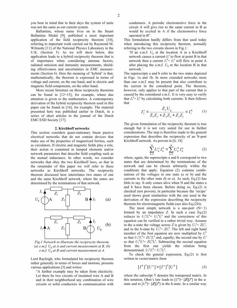
This section considers quasi-stationary linear passive electrical networks that do not contain devices that make use of the properties of magnetized ferrites, such as circulators. If electric and magnetic fields play a role, their action is contained in lumped elements and/or network parameters that describe field coupling such as the mutual inductance. In other words, we consider networks that obey the two Kirchhoff laws, so that in the remainder of this paper we will refer to these networks as Kirchhoff networks. The reciprocity theorem discussed here interrelates two states of one and the same Kirchhoff network, where the states are determined by the terminations of that network.

Fig.1 Network to illustrate the reciprocity theorem. (a) e.m.f. Ug at A and current measurement at B, (b)

e.m.f. Ug at B and current measurement at A. Lord Rayleigh, who formulated his reciprocity theorem rather generally in terms of forces and motions, presents various applications [3] and writes:

“A further example may be taken from electricity. Let there be two circuits of insulated wire A and B and in their neighborhood any combination of wire circuits or solid conductors in communication with

condensers. A periodic electromotive force in the circuit A will give rise to the same current in B as would be excited in A if the electromotive force operated in B”.

This formulation hardly differs from that used today when introducing this reciprocity theorem, normally referring to the two circuits shown in Fig.1:

‘If an e.m.f. Ug at the location A in a Kirchhoff network causes a current I2

a to flow at point B in that network then a current I1

b= I2a will flow in point A

after placing the e.m.f. Ug at the location B in that network.’

The superscripts a and b refer to the two states depicted in Figs. 1a and 1b. In more extended networks more than one e.m.f. may be present that also contribute to the current in the considered point. The theorem, however, only applies to that part of the current that is caused by the considered e.m.f.. It is very easy to verify that I1

b= I2a by calculating both currents. It then follows

that

(1) The given formulation of the reciprocity theorem is true enough but it is not very suited for use in further considerations. The step is therefore made to the general expression that describes the reciprocity of an N-port Kirchhoff network. As proven in [6, 18]

(2) where, again, the superscripts a and b correspond to two states that are determined by the terminations of the network and can be chosen arbitrarily within the conditions that apply. Equation (2) contains combi-nations of the voltages in one state (a or b) and the currents in the other state (b or a). As such, Eq.(2) has little to say. It only comes alive when N and the states a and b have been chosen. Before doing so, Eq.(2) is checked (not proven), in particular because the ‘recipe’ used shows great similarities with the one used in the derivation of the expression describing the reciprocity theorem for electromagnetic fields (see also Eq.(24)).

The most simple network is a one-port (N= 1) formed by an impedance Z. In such a case Eq.(2) reduces to U1

aI1b= U1

bI1a and the correctness of this

equation can be verified in a rather trivial way. Assume in the a-state the voltage across Z is given by U1

a= ZI1a,

and in the b-state by U1b= ZI1

b. The left and right hand member of the first equation are now multiplied by I1

b so that U1

aI1b= ZI1

aI1b and, equally, the second one by I1

a so that U1

bI1a= ZI1

bI1a. Subtracting the second equation

from the first one yields the relation being demonstrated: U1

aI1b= U1

bI1a.

To check the general expression, Eq.(2) is first written in vector/matrix form

(3)

where the subscript T denotes the transposed matrix. In this notation, Ohm’s law leads to [Ua]= [Z][Ia] in the a-state and to [Ub]= [Z][Ib] in the b-state. In a similar way

b1

133221

g3a2 Z

IZZZZZ

UZI =

++=

ak

N

1k

bk

bk

N

1k

ak IUIU ∑∑

==

=

][][][][ bTaaTb UIUI =

Ug

Ug

Z1 Z2 Z3

Z1 Z2 Z3

I1

I2

I1 I2

A

A

B

B

(a)

(b)

3

as with the one-port, the first equation is multiplied by [Ib]T and the second one by [Ia]T. The result of these multiplications is (note that the order of the terms is now always of importance)

(4a) and

(4b) where in Eq.(4b) we have made use of the matrix property [X]T[Y]T[Z]T= [Z][Y][X]T. If [Z]= [Z]T, as is the case in an N-port Kirchhoff network, Eq.(3) and hence Eq.(2) directly follow after subtracting Eq.(4b) from Eq.(4a).

3. Applications (1) This section presents four examples that connect the reciprocity theorem for Kirchhoff networks to EMC-measurements. The examples pay particular attention to the transfer impedance, filter attenuation, the conversion of a differential-mode (DM) voltage into a common-mode (CM) current and to site attenuation. In all examples Fig.2 applies and N= 2, but the applications are not limited to N= 2. For example, if cross-talk between parallel lines is considered, N= 3 or even higher may give useful information.

Fig.2 A two-port Kirchhoff network with a termination at each port that depends on the chosen application.

If N= 2, Eq.(2) reduces to

(5) In fact in Fig.1 N= 2 also applies. There U1

b= U2a= 0

and U1a= U2

b= Ug and substitution into Eq.(5) shows again that I1

b= I2a.

3.1 Transfer impedance The transfer impedance is the ratio of the voltage (e.m.f.) induced in a current loop by the current in another current loop. A typical example is the cable transfer impedance that characterizes the EMC behav-iour of a cable (the cable ‘leakage’). Fig.3 The two states when discussing the transfer

impedance

When applying Eq.(5), the termination at port 1 (see Fig.3) in the a-state is a current source of strength I1

a and port 2 is open circuited, i.e. I2

a= 0. In the b-state, a current source I2

b terminates port 2 while port 1 is open circuited, i.e. I1

b= 0. Hence, Eq.(5) reduces to U2aI2

b= U1

bI1a or, expressed in the transfer impedances Z12 and

Z21

(6) So the cable transfer impedance is reciprocal if the cable behaves as a Kirchhoff network. The cable is always passive and is always linear at most practical signal levels, as long there is no magnetic material in the cable construction. If magnetic material is used, the current (e.g. the CM current on the cable) must be verified to make sure that it is so low that no saturation of the magnetic material results. When measuring the transfer impedance it is often very difficult, if not impossible, to sufficiently satisfy the condition I1

b= 0 or I2a= 0 at high

frequencies, so that the measurement result has to be corrected for this non-zero current effect. Section 6.7 on interference prediction demonstrates another application of the transfer impedance concept. 3.2. Filter attenuation In the case of filter attenuation measurements, a source (e.m.f. Ug, internal impedance Zg) is connected via a filter to the load impedance ZL. A well known question related to filter attenuation is: ‘Does it matter which of the filter ports is connected to the source and which port is connected to the load of that source?’ If the filter itself is not purely symmetrical, the EMC engineer will answer that question with ‘Yes’, although he or she will not be able to demonstrate this using a 50Ω measuring system (generator and voltmeter having equal impedances, e.g. Zg= ZL= 50Ω). The latter can be verified as detailed below. Fig.4 The two states when discussing the filter

attenuation Assume that in the a-state port 1 is terminated by the source and port 2 by the load, and the reverse termination holds in state b (see Fig.4). If U0 is the voltage across ZL in the absence of the filter, the filter attenuation Aa= U2

a/U0 in the a-state and Ab= U1b/U0 in

the b-state. So here it is relevant to consider the ratio Aa/Ab= U2

a/U1b. At the terminations the following

relations are valid

(7a−7d)

]][[][][][ aTbaTb IIUI Z=

TaTTbbTabTa ][][][]][[][][][ IIIIUI ZZ ==

Kirchhoff

Network port

1 te

rmin

atio

n

U1 U2

I1 I2

+ +

− −

port 2 term

ination

a2

b2

a1

b1

b2

a2

b1

a1 IUIUIUIU +=+

120

b2

b1

0a1

a2

21b1

a2

ZI

UI

UZII

=====

La2

a2

Lb

1b

1

gb2g

b2

ga1g

a1

ZIU

ZIU

ZIUU

ZIUU

−=

−=

−=

−=I1a I2

bU2a U1

b

a-state b-state

Ug Ug

Zg Zg

ZL ZL

U2a U1

b

a-state b-state

4

From Eqs.(7c) and (7d) it follows that U2a/U1

b= I2a/I1

b and Eqs.(5) and (7) yield

(8) The attenuation will be independent of the choice of source port and load port if Aa/Ab= 1. In all other cases Aa/Ab≠ 1 and relative impedance values will determine the choice of the source and load port of the filter [19].

The condition Aa/Ab= U2a/U1

b= I2a/I1

b= 1 is met if I2

b=I1a and/or Zg= ZL. It is well known that the condition

I2b= I1

a, that simultaneously makes I2a= I1

b, is met in the case of a purely symmetrical filter; the reciprocity theorem was not needed to demonstrate this. However, the condition Zg= ZL resulting in Aa/Ab= 1 is sometimes overlooked as noted in Section 6.3. Moreover, it is this condition that explains why the engineer will measure no difference in the attenuation if source and load port are interchanged when using a 50Ω measuring system.

Of course, another path could also have been followed to arrive at the two conditions representing Aa= Ab. The Kirchhoff network can be characterized by a T-network and U2

a/U1b can be expressed in the

network impedances Z1, Z2 and Z3 (see Fig.1). After straight forward calculations it then follows that

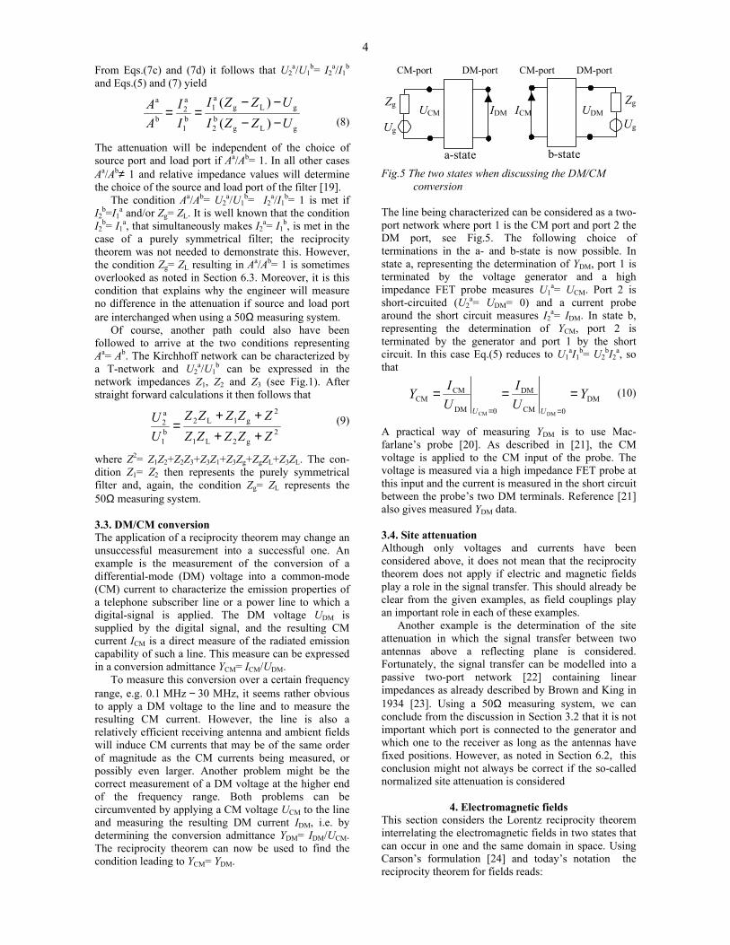
(9) where Z2= Z1Z2+Z2Z3+Z3Z1+Z3Zg+ZgZL+Z3ZL. The con-dition Z1= Z2 then represents the purely symmetrical filter and, again, the condition Zg= ZL represents the 50Ω measuring system. 3.3. DM/CM conversion The application of a reciprocity theorem may change an unsuccessful measurement into a successful one. An example is the measurement of the conversion of a differential-mode (DM) voltage into a common-mode (CM) current to characterize the emission properties of a telephone subscriber line or a power line to which a digital-signal is applied. The DM voltage UDM is supplied by the digital signal, and the resulting CM current ICM is a direct measure of the radiated emission capability of such a line. This measure can be expressed in a conversion admittance YCM= ICM/UDM.

To measure this conversion over a certain frequency range, e.g. 0.1 MHz − 30 MHz, it seems rather obvious to apply a DM voltage to the line and to measure the resulting CM current. However, the line is also a relatively efficient receiving antenna and ambient fields will induce CM currents that may be of the same order of magnitude as the CM currents being measured, or possibly even larger. Another problem might be the correct measurement of a DM voltage at the higher end of the frequency range. Both problems can be circumvented by applying a CM voltage UCM to the line and measuring the resulting DM current IDM, i.e. by determining the conversion admittance YDM= IDM/UCM. The reciprocity theorem can now be used to find the condition leading to YCM= YDM.

Fig.5 The two states when discussing the DM/CM

conversion The line being characterized can be considered as a two-port network where port 1 is the CM port and port 2 the DM port, see Fig.5. The following choice of terminations in the a- and b-state is now possible. In state a, representing the determination of YDM, port 1 is terminated by the voltage generator and a high impedance FET probe measures U1

a= UCM. Port 2 is short-circuited (U2

a= UDM= 0) and a current probe around the short circuit measures I2

a= IDM. In state b, representing the determination of YCM, port 2 is terminated by the generator and port 1 by the short circuit. In this case Eq.(5) reduces to U1

aI1b= U2

bI2a, so

that

(10) A practical way of measuring YDM is to use Mac-farlane’s probe [20]. As described in [21], the CM voltage is applied to the CM input of the probe. The voltage is measured via a high impedance FET probe at this input and the current is measured in the short circuit between the probe’s two DM terminals. Reference [21] also gives measured YDM data. 3.4. Site attenuation Although only voltages and currents have been considered above, it does not mean that the reciprocity theorem does not apply if electric and magnetic fields play a role in the signal transfer. This should already be clear from the given examples, as field couplings play an important role in each of these examples.

Another example is the determination of the site attenuation in which the signal transfer between two antennas above a reflecting plane is considered. Fortunately, the signal transfer can be modelled into a passive two-port network [22] containing linear impedances as already described by Brown and King in 1934 [23]. Using a 50Ω measuring system, we can conclude from the discussion in Section 3.2 that it is not important which port is connected to the generator and which one to the receiver as long as the antennas have fixed positions. However, as noted in Section 6.2, this conclusion might not always be correct if the so-called normalized site attenuation is considered

4. Electromagnetic fields This section considers the Lorentz reciprocity theorem interrelating the electromagnetic fields in two states that can occur in one and the same domain in space. Using Carson’s formulation [24] and today’s notation the reciprocity theorem for fields reads:

gLgb2

gLga1

b1

a2

b

a

)()(

UZZIUZZI

II

AA

−−−−

==

DM0CM

DM

0DM

CMCM

DMCM

YUI

UIY

UU

=====

Ug Ug

Zg ZgUCM UDMICM IDM

a-state b-state

CM-port CM-port DM-port DM-port

2g2L1

2g1L2

b1

a2

ZZZZZZZZZZ

UU

++++

=

5

“If Ea, Ha are the field vectors due to a periodic disturbance from a source A1 located at O1 and Eb, Hb are the corresponding field vectors due to a disturbance originating in A2 from a source located at O2, then

(11)

the surface integrals as indicated by the subscripts 1+2 being taken over closed surfaces 1 and 2 surrounding the sources A1 and A2 respectively.”

Not directly given in [24] is the additional equality also following from the reciprocity considerations

(12) where D is the volume containing the sources A1 and A2 represented by the source vectors Ja and Jb, res-pectively. In Eq.(11) the surface of D is indicated by the subscripts 1+2. Equation (12) will be used in the derivation of the hybrid reciprocity theorem in Section 5. As will be noted below, Eqs.(11) and (12) are connected to a special case of the general reciprocity relation Eq.(19).

So the theorem combines two field states (a and b), comparable to the discussed reciprocity theorem for an N-port Kirchhoff network. The derivation of Eqs. (11) and (12) starts from sets of two Maxwell’s equations expressed in the frequency domain for the states a and b:

(13a,b)

and

(14a,b) Now the trick is to remember the existence of the vector relation div(X×Y)=Y⋅curlX−X⋅curlY and to write

(15)

(16)

An expression for Hb⋅curlEa in Eq.(15) can be found by multiplying the left and right hand members of Eq.(13a) by Hb (be careful with the order of the variables)

(17)

In a similar way, expressions can be found for the other terms on the right hand side of Eqs.(15) and (16) by multiplying Eqs.(13b), (14a) and (14b) by the proper vectors. After substitution of all resulting expressions in Eqs.(15) and (16) and subtracting the two final equations, we find that

(18)

This equation, in which the ω-terms no longer appear, is sometimes called the local form of the reciprocity theorem. To find the general form, Eq.(18) has to be

integrated over the volume D containing all sources represented by Ja and Jb, yielding

(19)

We had to expect an integration as the Maxwell equat-ions consider field derivatives whereas an expression for the fields is needed. The most left hand member of Eq.(19) has been converted from an integral over a volume D into an integral over the surface S of D by applying Gauss’s theorem. This action also ‘removes’ the div operation. Equation (19) is the general form of the Lorentz reciprocity theorem, a form that can even be extended [14], although this extension is not needed in the context of this paper.

A special case is the situation in which the relation between the E and the H vector of the field is fixed, such as in the far-field of an antenna. Then the outcome of the integrals in Eq.(19) is equal to zero, a value given by Lorentz as he considered the propagation properties of light. In the far-field, the field propagates as a plane or quasi-plane wave so that the E and the H vector of the field are perpendicular to each other and have a constant ratio, η=√(µ/ε), the wave impedance (377 Ω in air). In vector notation the latter means that ν×E= ηH, where ν is the unit vector perpendicular to the plane formed by E and H. After application of this relation to Ea×Hb and to Eb×Ha and after application of the vector relation X×(Y×Z)= Y⋅(X⋅Z)−Z(X⋅Y) we find that

(20)

so that abba HEHE ×−× = 0 and, consequently, the integrals in Eq.(19) are equal to zero and Eqs.(11) and (12) given at the start of this section automatically follow.

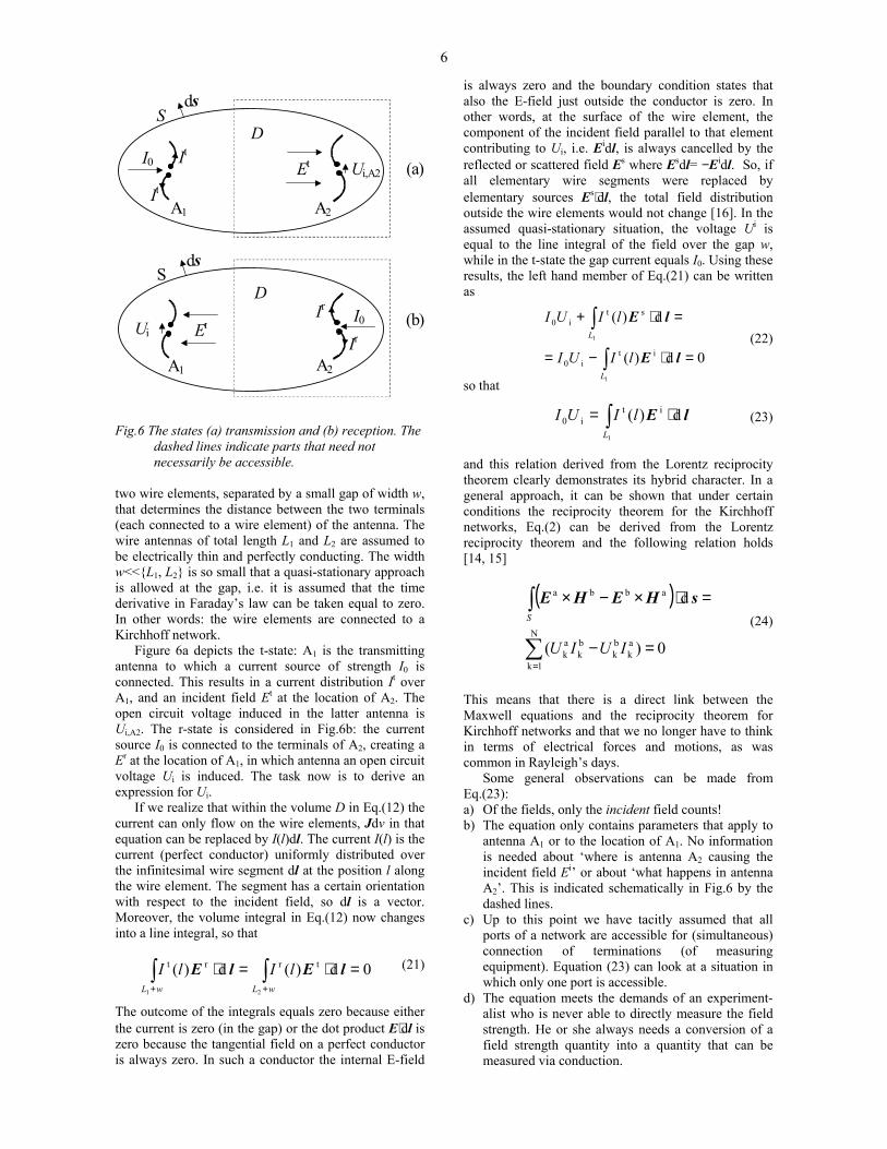
5. The hybrid reciprocity theorem The experimentalist can only humbly lift his hat at the mathematical fireworks presented in Section 4 and then pass to the order of the day. An application is what is needed to catch his or her interest. As mentioned in the introduction, a very useful application was already given in 1929 by Ballantine [10], referring to the work of Wilmotte [11].This application, resulting in the hybrid reciprocity theorem, can also be found in Section 4.5 of a more recent textbook [16]. The theorem gives an expression for the voltage Ui induced by an incident field Ei in an antenna or structure acting as an antenna, e.g. an EUT (Equipment Under Test) and its connected cables. Since the transmission and reception of electromagnetic waves is of interest in EMC field measurements, the two states a and b will now be denoted by t (of transmission) and r (of reception).

In the following, two wire antennas A1 and A2 are considered (see Fig.6). Each wire antenna consists of

sHEsHE d)(d)(21

ab

21

ba ∫∫++

⋅×=⋅×

∫∫ ⋅=⋅DD

vv d)(d)( abba JEJE

aaa

aa

curlcurl

JEHHE

++=

−=

εωµω

jj

bbb

bb

curlcurl

JEHHE

++=−=

εωµω

jj

baabba curlcurl)(div HEEHHE ⋅−⋅=×

abbaab curlcurl)(div HEEHHE ⋅−⋅=×

abab curl HHEH ⋅−=⋅ µωj

( ) baababbadiv JEJEHEHE ⋅−⋅=×−×

( )( )( )∫

∫

∫

⋅⋅−⋅

=⋅×−×

=⋅×−×

D

S

D

vJEJE

sHEHE

vHEHE

d

d

ddiv

baab

abba

abba

)( ababba EEHEHE ⋅=×=× η

6

Fig.6 The states (a) transmission and (b) reception. The

dashed lines indicate parts that need not necessarily be accessible.

two wire elements, separated by a small gap of width w, that determines the distance between the two terminals (each connected to a wire element) of the antenna. The wire antennas of total length L1 and L2 are assumed to be electrically thin and perfectly conducting. The width w<<L1, L2 is so small that a quasi-stationary approach is allowed at the gap, i.e. it is assumed that the time derivative in Faraday’s law can be taken equal to zero. In other words: the wire elements are connected to a Kirchhoff network.

Figure 6a depicts the t-state: A1 is the transmitting antenna to which a current source of strength I0 is connected. This results in a current distribution It over A1, and an incident field Et at the location of A2. The open circuit voltage induced in the latter antenna is Ui,A2. The r-state is considered in Fig.6b: the current source I0 is connected to the terminals of A2, creating a Er at the location of A1, in which antenna an open circuit voltage Ui is induced. The task now is to derive an expression for Ui.

If we realize that within the volume D in Eq.(12) the current can only flow on the wire elements, Jdv in that equation can be replaced by I(l)dl. The current I(l) is the current (perfect conductor) uniformly distributed over the infinitesimal wire segment dl at the position l along the wire element. The segment has a certain orientation with respect to the incident field, so dl is a vector. Moreover, the volume integral in Eq.(12) now changes into a line integral, so that

(21) The outcome of the integrals equals zero because either the current is zero (in the gap) or the dot product E⋅dl is zero because the tangential field on a perfect conductor is always zero. In such a conductor the internal E-field

is always zero and the boundary condition states that also the E-field just outside the conductor is zero. In other words, at the surface of the wire element, the component of the incident field parallel to that element contributing to Ui, i.e. Eidl, is always cancelled by the reflected or scattered field Es where Esdl= −Eidl. So, if all elementary wire segments were replaced by elementary sources Es⋅dl, the total field distribution outside the wire elements would not change [16]. In the assumed quasi-stationary situation, the voltage Ui is equal to the line integral of the field over the gap w, while in the t-state the gap current equals I0. Using these results, the left hand member of Eq.(21) can be written as

(22)

so that

(23)

and this relation derived from the Lorentz reciprocity theorem clearly demonstrates its hybrid character. In a general approach, it can be shown that under certain conditions the reciprocity theorem for the Kirchhoff networks, Eq.(2) can be derived from the Lorentz reciprocity theorem and the following relation holds [14, 15]

(24) This means that there is a direct link between the Maxwell equations and the reciprocity theorem for Kirchhoff networks and that we no longer have to think in terms of electrical forces and motions, as was common in Rayleigh’s days.

Some general observations can be made from Eq.(23): a) Of the fields, only the incident field counts! b) The equation only contains parameters that apply to

antenna A1 or to the location of A1. No information is needed about ‘where is antenna A2 causing the incident field Ei’ or about ‘what happens in antenna A2’. This is indicated schematically in Fig.6 by the dashed lines.

c) Up to this point we have tacitly assumed that all ports of a network are accessible for (simultaneous) connection of terminations (of measuring equipment). Equation (23) can look at a situation in which only one port is accessible.

d) The equation meets the demands of an experiment-alist who is never able to directly measure the field strength. He or she always needs a conversion of a field strength quantity into a quantity that can be measured via conduction.

0d)(d)(21

trrt =⋅=⋅ ∫∫++ wLwL

lIlI lElE

∫

∫

=⋅−=

=⋅+

1

1

0d)(

d)(

iti0

sti0

L

L

lIUI

lIUI

lE

lE

∫ ⋅=1

d)( iti0

L

lIUI lE

( )

0)(

d

N

1k

ak

bk

bk

ak

abba

=−

=⋅×−×

∑

∫

=

IUIU

S

sHEHE

I0 Ui,A2

A1 A2 It

It Et

Ir

Ir

I0Er Ui

A1 A2

D

D

S

S ds

ds

(a)

(b)

7

e) Equation (23) can also be written as

(25)

so that It(l)/I0 can be considered to be the normalized current distribution in the transmitting state that weighs the contributions of incident field in the receiving state.

6. Applications (2) This section presents a number of simple applications of Eq.(23) or Eq.(25), dealing with the antenna factor, radiated immunity measurements and shielding. Interesting and rigorously treated applications of Eq.(24) can be found in [15, 25]. Only in simple cases can the integral in Eq.(23) or Eq.(25) be solved analytically; an example is given in Section 6.1. However, the other examples will show that quite useful information is made available without solving the integral. 6.1. The λ/2-dipole A very simple application of Eq.(25) follows if we calculate the voltage induced in a λ/2-dipole in free space. As can be found in all current text books on antennas and was verified experimentally by Wilmotte in 1927 [26], the current distribution in the transmitting state of this antenna is half a sine wave. If the incident field is a plane wave of strength Ei with its polarization parallel to the wire elements, the well known expression for the induced voltage follows from Eq.(25):

(26)

If Zm is the effective load impedance and Za the internal impedance of the λ/2-dipole antenna, the voltage Um measured by the receiver is given by

(27) and if Ei= Ec

i is the field strength during calibration of this antenna, its antenna factor FA is given by

(28) By stating ‘Zm is the effective load impedance of the antenna’ and not ‘Zm is the input impedance of the receiver’, the properties of the antenna balun are assumed to be taken into account.

Seibersdorf, for example, is a supplier of a set of 27 λ/2-dipole antennas suitable for performing the validation of an antenna calibration test site as described by CISPR/A [27]. For these antennas Zm= 100 Ω, and the free space value of Za= 73 Ω. Inserting these values in Eq.(28) results in FA values that differ less than 0.1 dB from the theoretical values supplied by Seibersdorf (maybe, Seibersdorf also used Eq.(28)).

6.2. The antenna factor FA This section should clarify which parameters play a role in the determination of the antenna factor and what the consequences are in radiated emission measurements, measurement uncertainty and normalized site attenuation measurements.

By definition, the measured field strength Em= FAUm, so the antenna factor can be written as

(29) The antenna factor therefore depends on 3 variables determined by the calibration set-up, in Eq.(29) indicated by the subscript c, 1) The antenna impedance Za,c, 2) The normalized current distribution Ic

t(l)/I0, and 3) The outcome of the dot-product Ec

i⋅dl along the wire elements.

As a consequence, if in a radiated emission measure-ment one or more of these three variables differ from the values during calibration, the antenna factor is unknown. In discussions about the standardization of radiated emission tests, the first variable (the antenna impedance) has often been considered, but not the other two variables.

The normalized current distribution depends on the interaction of the antenna with its environment during its actual use (calibration or radiated emission test). Of course, the outcome of the integral depends on the incident-field distribution which, however, is not specified in a radiated emission compliance test. The wire elements of a receiving antenna automatically ‘integrate’ over the field distribution whether the measurement is carried out on an open area test site, or in a semi or a fully anechoic room. Consequently, antennas with different shapes will have different induced voltages, even if the incident field is a plane wave.

Fig 7. The difference ∆FA= FA(ANSI/3m)−FA(Free-

Space) between the antenna factors of a log-biconical antenna derived from the two calibration reports

The combined effect of all three variables comes to the fore in the first example. Figure 7 shows the difference ∆FA between the ANSI(3m) antenna factor and the free-

∫ ⋅=1

d)( i

0

t

iL I

lIU lE

∫−

=−=4/

4/

i0

0

i

i d))4

(2sin(λ

λ πλλ

λπ EllI

IEU

i

am

mm π

EZZ

ZU λ+

=

m

amA

)π(Z

ZZFλ

+=

∫ ⋅

+=

L

IlIZZZ

FlE d)/)((

1ic0

tcm

ca,mA

0,0

0,5

1,0

1,5

2,0

2,5

0 50 100 150 200 250 300

Frequency (MHz)

∆FA (

dB)

8

space antenna factor of one and the same log-biconical antenna, as determined by a UKAS accredited company.

We can also conclude from the above that the linearized model used in documents on EMC measurement instrumentation uncertainties [28, 29] cannot be justified. Moreover, the uncertainty in the antenna factor during calibration has little in common with the uncertainty in the antenna factor during an actual radiated emission test. In the normalized site attenuation measurement method the result of the site attenuation measurement is normalized to the antenna factors, after which the result is compared to a theoretically predicted result. This method is formally only correct if it can be demonstrated that the antenna factors used are valid during the conditions of the site attenuation measurement.

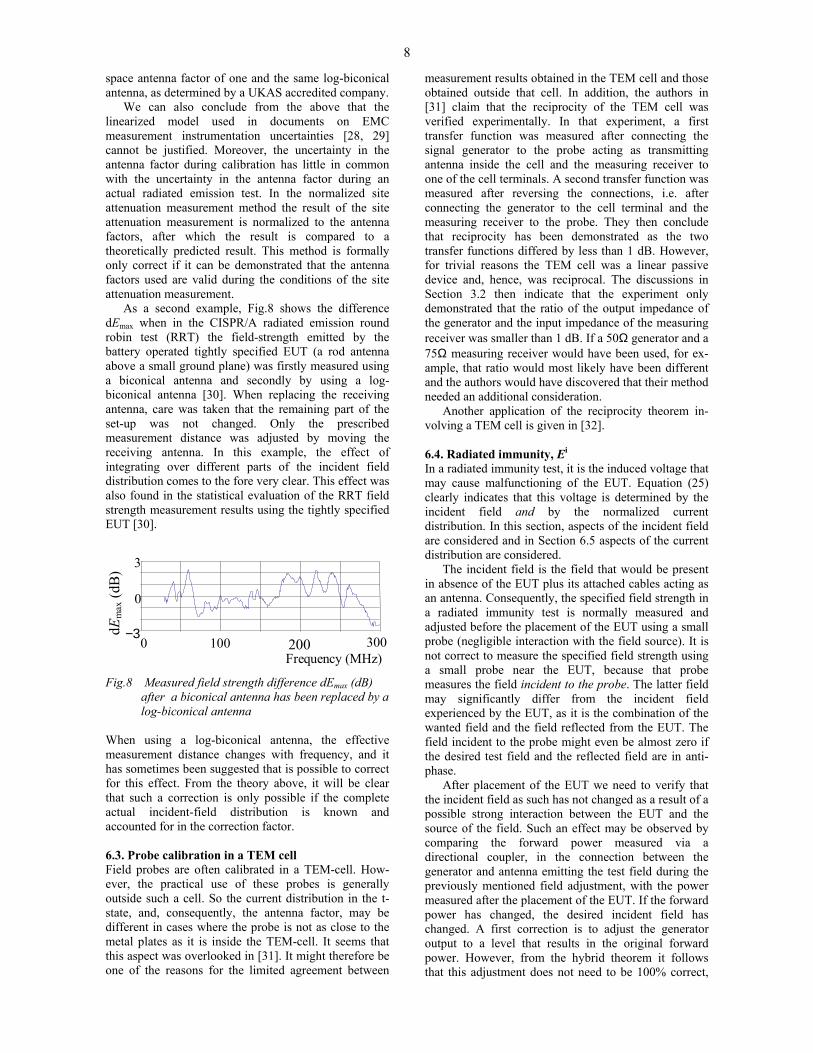
As a second example, Fig.8 shows the difference dEmax when in the CISPR/A radiated emission round robin test (RRT) the field-strength emitted by the battery operated tightly specified EUT (a rod antenna above a small ground plane) was firstly measured using a biconical antenna and secondly by using a log-biconical antenna [30]. When replacing the receiving antenna, care was taken that the remaining part of the set-up was not changed. Only the prescribed measurement distance was adjusted by moving the receiving antenna. In this example, the effect of integrating over different parts of the incident field distribution comes to the fore very clear. This effect was also found in the statistical evaluation of the RRT field strength measurement results using the tightly specified EUT [30].

Fig.8 Measured field strength difference dEmax (dB) after a biconical antenna has been replaced by a log-biconical antenna

When using a log-biconical antenna, the effective measurement distance changes with frequency, and it has sometimes been suggested that is possible to correct for this effect. From the theory above, it will be clear that such a correction is only possible if the complete actual incident-field distribution is known and accounted for in the correction factor. 6.3. Probe calibration in a TEM cell Field probes are often calibrated in a TEM-cell. How-ever, the practical use of these probes is generally outside such a cell. So the current distribution in the t-state, and, consequently, the antenna factor, may be different in cases where the probe is not as close to the metal plates as it is inside the TEM-cell. It seems that this aspect was overlooked in [31]. It might therefore be one of the reasons for the limited agreement between

measurement results obtained in the TEM cell and those obtained outside that cell. In addition, the authors in [31] claim that the reciprocity of the TEM cell was verified experimentally. In that experiment, a first transfer function was measured after connecting the signal generator to the probe acting as transmitting antenna inside the cell and the measuring receiver to one of the cell terminals. A second transfer function was measured after reversing the connections, i.e. after connecting the generator to the cell terminal and the measuring receiver to the probe. They then conclude that reciprocity has been demonstrated as the two transfer functions differed by less than 1 dB. However, for trivial reasons the TEM cell was a linear passive device and, hence, was reciprocal. The discussions in Section 3.2 then indicate that the experiment only demonstrated that the ratio of the output impedance of the generator and the input impedance of the measuring receiver was smaller than 1 dB. If a 50Ω generator and a 75Ω measuring receiver would have been used, for ex-ample, that ratio would most likely have been different and the authors would have discovered that their method needed an additional consideration.

Another application of the reciprocity theorem in-volving a TEM cell is given in [32]. 6.4. Radiated immunity, Ei In a radiated immunity test, it is the induced voltage that may cause malfunctioning of the EUT. Equation (25) clearly indicates that this voltage is determined by the incident field and by the normalized current distribution. In this section, aspects of the incident field are considered and in Section 6.5 aspects of the current distribution are considered.

The incident field is the field that would be present in absence of the EUT plus its attached cables acting as an antenna. Consequently, the specified field strength in a radiated immunity test is normally measured and adjusted before the placement of the EUT using a small probe (negligible interaction with the field source). It is not correct to measure the specified field strength using a small probe near the EUT, because that probe measures the field incident to the probe. The latter field may significantly differ from the incident field experienced by the EUT, as it is the combination of the wanted field and the field reflected from the EUT. The field incident to the probe might even be almost zero if the desired test field and the reflected field are in anti-phase.

After placement of the EUT we need to verify that the incident field as such has not changed as a result of a possible strong interaction between the EUT and the source of the field. Such an effect may be observed by comparing the forward power measured via a directional coupler, in the connection between the generator and antenna emitting the test field during the previously mentioned field adjustment, with the power measured after the placement of the EUT. If the forward power has changed, the desired incident field has changed. A first correction is to adjust the generator output to a level that results in the original forward power. However, from the hybrid theorem it follows that this adjustment does not need to be 100% correct,

−3

0

3

0 100 200 300Frequency (MHz)

dEm

ax (d

B)

9

as the field distribution during the field adjustment and that after placement of the EUT need not be the same. 6.5. Radiated immunity, It(l)/I0 Equation (25) also indicates that the normalized current distribution in the t-state is of importance. Since that distribution is the weighting function of the voltage contributions induced by the incident field, resonances in that distribution may be noticed in the disturbance signal induced in the cable attached to an EUT. An example is given in Fig.9, where the maximum (max), average (avg) and the minimum (min) value of the measured induced CM-current are plotted as a function of the frequency of the homogeneous incident field with a strength of 1 V/m. Eight EUTs taken from a class of electrically small EUTs were tested [21]. Fig.9 The induced common-mode current measured

close to an electrically small EUT in the cable attached to that EUT, when illuminated by a field of 1 V/m (8 EUTs)

Although the average value is about 55 dBµA (a value close to the rule of thumb for these EUTs: 1 mA per V/m), the curve labelled ‘min’ indicates that resonances may cause a minimum in the induced current, so that the considered EUT is hardly tested for immunity around the resonance frequencies. In other words, a uniform and constant incident field does not guarantee that the EUT is tested with a constant actual disturbance signal (here represented by the CM current). In addition, we should expect the resonance frequencies to shift when the layout of the cables is changed. If it had been possible to let the EUT act as a transmitter, the resonances would also have been found, comparable to the resonances of a rod antenna.

In the case of an interference complaint in which a product is insufficiently immune to EM fields, it is not always possible to solve the problem at the location where the product is used. The disturbance field strength at that location is measured and the product is taken to the test lab to carry out a radiated immunity test with that field strength. However, if the CM current distribution on the cables attached to that product differs significantly in the test situation from that at the complaint location, the test might not cover the actual complaint. So it is advisable to measure not only the field strength at the complaint location, but also the CM current on the attached cables (close to the product) and

to verify whether these currents are (more or less) the same in the test house. 6.6. Shielding This section addresses the frequently asked question ‘If a shield attenuates the field emanating from circuits inside that shield by an amount of X dB, are these circuits then also shielded by an amount of X dB for fields generated outside that shield?’ We can illustrate the reasoning behind the answer by the following rather simple configuration, that allows the use of simple analytical relations. Rigorous approaches based on the Lorentz theorem can be found in [25, 33]. In Section 6.7 the results are also used in an example of interference prediction. Fig.10 Schematic drawing for use in the application of

the reciprocity theorems A tuned λ/2 dipole is located at a distance r in the far-field of a small loop antenna, as shown in Fig.10. Both antennas are located in free space so that antenna coupling and reflections do not play a role. A signal source Ug, Rg can be connected to the loop antenna, and a voltmeter (input impedance Rv= Rg) can be connected to the λ/2 dipole (internal impedance Za), and vice versa. The area of the loop antenna A= πDa

2/4 and the internal impedance of that antenna is Zl. The orientation of both antennas is such that an optimal signal transfer results.

If the source is connected to the loop antenna and the voltmeter to the λ/2 dipole, the voltmeter reading Uv1 in the absence of the screen will be given by

(30) where λRg/π(Rg+Za)is the voltmeter reading in the case of an incident field given by the second part of the right hand member of Eq.(30), (also see Eq. (27)). In that part, AUg/(Rg+Zl) is the magnetic dipole moment of the loop antenna, Z0 the far-field wave impedance and k= 2π/λ. Next, a spherical screen of radius R, Da/2<<R<<r, λ/2π, is put around the loop antenna such that the loop is in its center. The screen is assumed to be in the near field of the loop. Now the voltmeter reading is Uv2 and, consequently, the shielding effectiveness SH= Uv1/Uv2. Because the sphere also acts as a magnetic dipole [25], Uv2 is also described by

max

min

avg

0 50 100 150 20020

40

60

80

Frequency (MHz)

CM

-cur

rent

dB(

µA)

+

Screen

λ/2-antennaLoop antenna

Da

R

r

)(π4)(π g

g2

0

ag

gv1 ZRr

UAkZZR

RU

+⋅

+=

λ

10

Eq.(30), although the magnetic dipole moment is now a factor SH smaller.

The next step is to connect the generator to the λ/2 dipole and the voltmeter to the loop antenna. In the absence of the screen Uv3 is measured and in the presence of that screen Uv4 is measured. The voltage Uv3 is given by

(31) where Rg/(Rg+Zl) gives the voltage division of the voltage µ0ωAH induced by the incident H-field. That field is given by the second part of the right hand member of Eq.(31), and is easily understood when remembering that in the far-field the E-field of a center fed tuned λ/2 dipole is given by E= 60I/r= 2Z0/(4πr) so that H= 2I/(4πr) and where I is the current entering the antenna.

Using the relations Z0= √(µ0/ε0) and f⋅λ = c = 1/√(µ0ε0) we can easily verify that Uv1= Uv3. This is not a surprising result, since the equivalent network between the ports of the two antennas is a Kirchhoff network, which means that the associated reciprocity theorem directly gives the answer Uv1= Uv3 (see Eq.(8)) using Zg= ZL= Rg. However, because the screen is also linear and passive, the same theorem shows that Uv2= Uv4, and a simple calculation like the one above to demonstrate this result is not possible. The last statement is particularly true because the dipole field arrives as a plane wave at the screen, while the screen is in the near-field region of the loop antenna. A knowledgeable in the theory may be able to show that the Helmholtz theorem about the reversibility of light rays [2] is applicable in the described situation.

In this example the actual shielding effectiveness is determined by that of the screen in the near-field of the loop antenna. This effectiveness is generally much lower, e.g. 40 dB, than that for a plane wave generated outside the screen. The example stresses the fact that the shielding effectiveness is not entirely a property of the shield. It is a property of the shield plus the antennas or antenna structures playing a role in the disturbance signal transfer.

In conclusion, the reciprocity theorems give con-ditions under which the shielding effectiveness is reciprocal, and the results are certainly applicable in the case of in-band interference. In the case of out-of-band disturbances acting on non-linear devices such as transistors, the theorems are not formally applicable. However, it is still possible to follow the given path to estimate the magnitude of the induced signals and to consider the consequences of those signals afterwards [33]. 6.7. Interference prediction The results obtained in Section 6.6 can be applied to interference prediction. As an example, the following application considers the unwanted signal induced by a distant broadcasting transmitter in the antenna of

Magnetic Resonance Imaging (MRI) equipment used in hospitals.

In the early days of the use of MRI equipment, hospitals did not like to have large Faraday cages around the equipment. As broadcasting transmitters could emit strong fields at the in-band frequencies of the MRI equipment, the following question arose ‘Is it possible to carry out field strength measurements at the location where the MRI equipment is planned to be used before the placement of that equipment and to predict the level of the disturbance signal induced in the MRI antenna?’ The answer was ‘Yes, and with a reasonable degree of confidence’. The following three steps had to be followed to find the answer. Figure 10 is again applicable: the MRI antenna is the loop antenna and the λ/2 dipole is the antenna of the broadcasting transmitter, (normally a λ/4 antenna above the earth acting as a ground plane). Simple mathematical relations illustrate the estimate of the maximum voltage Ui,max that could be induced in the loop antenna.

Step 1: Connect a signal source Ug, Rg to the MRI antenna located at its normal-use position inside the MRI equipment, so that all interactions are properly taken into account. Set the frequency of this source to that of the (strong) broadcasting field to be expected in the hospital. Measure at a distance r1 in the far-field of the MRI equipment the field pattern E1(φ), 0°≤φ≤360°, emitted by the MRI antenna and measure the current I0

t flowing into the loop antenna. This is a measurement that can be carried out on the manufacturers premises!

Step 2: Determine the maximum Emax of E1(φ) and assume that the MRI equipment emits this field in the direction of the λ/2 dipole at a distance r from the equipment (worst case). This field is proportional to I0

t, so Emax= αmaxI0

t and the incident field for the λ/2 dipole Et= (αr1I0

t)/r. Application of the hybrid reciprocity theorem then gives the voltage induced in the λ/2 dipole: Ui,λ/2= (αmaxλr1I0

t)/(πr), (see Eq.(26)). Conse-quently, the transfer impedance Ztr between the loop antenna and the λ/2 dipole is given by

(32)

and in the given situation Ztr is reciprocal.

Step 3: During operation of the broadcasting transmitter, the input current to its antenna is I0

r and that current can be determined from the field strength Er measured at the location where the MRI equipment is to be installed, by using the well known relation Er= 60I0

r/r. Using Eq.(32), the estimate of the maximum voltage Ui,max induced by the broadcasting transmitter in the loop antenna is given by

(33)

By comparing this voltage with the level allowed to operate the MRI equipment sufficiently free of interference, a decision can be made about whether or not a Faraday cage is needed and, if it is, how much attenuation that cage should present.

)(π42

)( ag

g

g

g03v ZRr

UZR

ARU

+⋅

+=

ωµ

rrZ

πλα 1max

tr =

r1maxr0trmax,i 60

ErIZUπλα==

11

Summary In this paper we have discussed the reciprocity theorem interrelating two states of one and the same Kirchhoff network (linear passive network) as determined by the terminations of that network. We have given applications improving the understanding of transfer impedance, filter and site attenuation measurements. In addition, we have used the theorem to facilitate a DM voltage to CM current conversion measurement.

We discussed the reciprocity theorem interrelating the electromagnetic fields in two states that can occur in one and the same domain in space, and from this theorem we derived the hybrid reciprocity theorem. The latter theorem was applied to a tuned λ/2 dipole, to the measurement of antenna factors, to probe calibration in a TEM cell and the uncertainties associated with these measurements. We also used the hybrid reciprocity theorem to discuss aspects of radiated immunity measurements.

Finally, we used the reciprocity the reciprocity theorems in a discussion about the reciprocity of the shielding effectiveness and in a simple method to estimate the interference potential of a field (at in-band frequencies) incident on an antenna. Acknowledgements The author wishes to acknowledge the valuable and interesting discussions with Dr. Stef Worm of Philips EMC Competence Centre in Eindhoven. He also wishes to thank the library staff at Philips Research in Eind-hoven. The presence of all historical publications in the library’s collection made his nostalgic journey a pleas-ant ‘one-stop’ event. References [1] S. Ballantine, “The Lorentz Reciprocity Theorem

for Electric Waves”, Proc. IRE, vol.16, pp 513− 518, 1928.

[2] H. von Helmholtz, Handbuch der Physiologischen Optik (1866); Verlag von Leopold Voss, Ham-burg/Leipzig, 3e Auflage, pp 200−203, 1909.

[3] J.W. Strutt, Baron Rayleigh, The theory of sound, vol. 1, pp. 150−157, 1877; reprinted by Mac-Millan, London, 1926.

[4] H.A. Lorentz, “Het theorema van Poynting over de energie van het electromagnetisch veld en een paar algemene stellingen over de voortplanting van het licht”, Verslagen Kon. Akademie van Wetenschap-pen, Band 4, p.176, Amsterdam, 1896.

[5] H.A. Lorentz, “The theorem of Poynting con-cerning the energy in the electromagnetic field and two general propositions concerning the propagation of light”, Collected papers, Nijhoff, Den Haag, vol. III, p 1, 1936.

[6] J.R. Carson, “A generalization of the reciprocal theorem”, Bell Syst. Techn. Jrnl., vol. 3, pp 393− 399, July 1924.

[7] A. Sommerfeld, “Das Reziprozitäts-Theorem der drahtlosen Telegraphie”, Zeitschrift für Hoch-frequenztechnik, Band 26, Heft 4, pp 93−98, 1925.

[8] M. Abraham, Theorie der Elektrizität, Teubner Verlag, Berlin, 1921.

[9] The Stuart Ballantine Medal, to be awarded in recognition of outstanding achievement in the fields of Communication and Reconnassance which employ electromagnetic radiation, The Franklin Institute, Philadelphia, U.S.A.

[10] S. Ballantine, “Reciprocity in electromagnetic, mechanical, acoustical, and interconnected systems”, Proc. IRE, vol. 17, pp 929-951, June 1929.

[11] R.M. Wilmotte, “The nature of the field in the neighbourhood of an antenna”, Journ. IEE, vol. 66, pp. 961−967, 1928.

[12] C.T. Tai, “Complementary Reciprocity Theorems for Two-Port Networks and Transmission Lines”, IEEE Trans. on Education, vol. 37, no.1, pp 42−45, 1992.

[13] C.T. Tai, “Complementary Reciprocity Theorems in Electromagnetic Theory”, IEEE Trans. on Antennas and Propagation, vol.40, no.6, pp 675−681, 1992.

[14] A.T. de Hoop, Handbook of radiation and scattering of waves, Academic Press Ltd., London, 1995.

[15] D. Quak, “Electromagnetic Susceptibility Analysis of Open-Wire Systems”, Proc. IEEE Intern. Symp. on EMC, Atlanta, pp 423−428, August 1995.

[16] K.F. Sander and G.A.L. Reed, Transmission and propagation of electromagnetic waves, Cambridge University Press, Cambridge, 1986.

[17] J.J. Goedbloed, “Reciprociteit en EMC-metingen”, EMC/ESD Praktijk, 1) pp.5−7, Sept. 2001, 2) pp 5−7, Okt. 2001, 3) Elektronica, EMC/ESD Prak-tijk, pp. 5−7, Nov. 2001, “Over het afschermen van velden (4)”, Elektronica, EMC/ESD Praktijk, pp. 44−45, Mei 2002.

[18] B.D.H. Tellegen, “A general network theorem, with applications”, Philips Research Reports, 7, pp259−269, 1952.

[19] J.J. Goedbloed, Electromagnetic Compatibility, Kluwer Technische Boeken, Deventer, 1997 (orig-inally published by Prentice Hall, 1992).

[20] I.P. Macfarlane, “A Probe for the Measurement of Electrical Unbalance of Networks and Devices”, IEEE Trans. on EMC, vol. 41, pp. 3−14, Feb. 1999.

[21] J.J. Goedbloed, “Aspects of EMC at the equipment level”, Proc. Intern. Symp. on EMC, Zurich, Suppl. pp 23−38, 1997 and IEEE Intern. EMC Sym-posium, Austin, U.S.A., 1997.

[22] A. Sugiura, “Formulation of Normalized Site Attenuation in Terms of Antenna Impedances”, Trans. IEEE on EMC, vol. 32, pp. 257−263, Nov. 1990.

[23] G.H. Brown and R. King, “High frequency models in Antenna investigations”, Proc. IEE, vol. 22, pp. 457−480, April 1934.

[24] J.R. Carson, “Reciprocal theorems in radio com-munication”, Proc.IRE, vol.17, pp 952-956, June 1929.

[25] D. Quak and A.T. de Hoop, “Shielding of Wire Segments and Loops in Electric Circuits by

12

Spherical Shells”, Trans. IEEE on EMC, vol. 31, pp 230− 237, August 1989.

[26] R.M. Wilmotte, “The distribution of current in a transmitting antenna”, Jour. I.E.E., vol. 66, pp 617− 627, 1928.

[27] Specification for radio disturbance and immunity measuring apparatus, CISPR Publ. 16-1, 2nd Ed., pp 107-133, 1999.

[28] Accounting for the measurement uncertainty when determining compliance with a limit, CISPR Publ. 16-4, 2002.

[29] The treatment of uncertainty in EMC measure-ments, NAMAS Publication NIS81, May 1994

[30] J.J. Goedbloed, “Analysis of the results of the

CISPR/A radiated emission round robin test”, Nat. Lab. Unclassified Report 2002/811, May 2002, Philips Research, Eindhoven, The Netherlands.

[31] D.J. Groot Boerle, F.B.J. Leferink and T.D. Leisti-kow, “Obtaining the antenna factor of an optically driven antenna using the reciprocity of a TEM cell”, IEEE EMC Symposium, pp 900−905, 1998.

[32] S.B. Worm, Comparison of workbench methods for testing RF emission properties of integrated circuits, Proc. Intern. Symp. on EMC, Zurich, pp 673−678, Febr. 2001.

[33] B.L. Michielsen, “A new approach to electromag-netic shielding”, Proc. Inter. Symp. on EMC, Zurich, pp 509−514, March 1985.