Dipartimento di Scienze Economiche e Sociali

UNIVERSITÀ POLITECNICA DELLE MARCHE

Reciprocity in the labor market:

experimental evidence

Annarita Colasante, Alberto Russo

QUADERNI DI RICERCA n. 404ISSN:2279-9575

August 2014

Comitato scientifico:

Renato BalducciMarco GallegatiAlberto NiccoliAlberto Zazzaro

Collana curata da:Massimo Tamberi

Abstract

In this paper we focus on the impact of involuntary unemployment on wageformation using experimental evidence. We use the well-known Gift Ex-change Game to analyze players’ interaction in a simplified job market. Theaim of this paper is twofold: on the one hand, we are interested in analyz-ing the relation between involuntary unemployment and wages; on the otherhand, we aim at understanding whether the interaction between employersand employees could be affected by reciprocity. Our results show that un-employment has a negative impact on wages. Moreover, there is a positivecorrelation between wage and effort.

JEL Class.: C91, E24, J28, J30Keywords: Reciprocity, Gift Exchange, Unemployment

Indirizzo: Dipartimento di Scienze Economiche e Sociali,Universita Politecnica delle Marche. E-mail:a.colasante@univpm.it

Contents

1 Introduction 1

2 Experimental Setting 3

3 Experimental results: descriptive statistics and graphical anal-ysis 7

4 Estimation results 14

5 Conclusion and future analysis 19

A Experiments using z-tree: Gift Exchange Game 23

Reciprocity in the labor market:experimental evidence∗

Annarita Colasante, Alberto Russo

1 Introduction

In this paper we analyze the labor market using experimental evidence inorder to understand the relation between unemployment and wages. In par-ticular, we focus on the impact of exogenous excess of labor supply on bothwage and effort. The aim of this paper is twofold: on the one hand, wecheck if involuntary unemployment has a negative impact on wages; on theother hand, we are interested in understanding if the interaction betweenemployers and employees could be affected by reciprocity 1.

We gathered experimental evidence using the well known Bilateral GiftExchange Game developed by Fehr et al. (1993). In this game participantsplay in the role of employer or employee and they interact in a simplified jobmarket. In the baseline form of the Bilateral Gift Exchange Game playersare randomly assigned to the role of employers or employees. Interactionbetween the two parties can be summarized by a two stage game. Usually,in the first stage, employers propose a single contract consisting in a wagew and a desired effort e. Workers observe all the feasible contracts andthey can accept one of these offers or not. In the second step, workerswho subscribe a contract must choose their effective level of effort e. Eachemployee can choose a level of effort lower than the required one (e < e),fulfill the contract (e = e) or an effort level greater than the proposed one(e > e). In the standard game there is no punishment or reward for any levelof effort different from the required level.

Using a similar setting, we try to validate our hypotheses, which is thatfirms are willing to pay low wages in a market with a high unemployment

∗ The authors gratefully acknowledge the Polytechnic University of Marche and Profes-sor Alessandro Sterlacchini for the financial support. We wish to thank the technical staff,especially Daniele Ripanti. We are grateful to Matteo Picchio for helpful suggestions.

1As in Falk and Fischbacher (2006), reciprocity is a behavioral response to perceivedkindness.

1

rate and that players are strongly influenced by the counterpart’s behavior.Moreover, we take into account the impact of risk aversion on individualchoices. In fact, we assign players with high risk aversion to the role ofemployee and we try to measure the impact of the risk aversion on finalgains.

Under the hypothesis of perfect rationality, the best strategy for employ-ees is to choose the minimum level of effort, while the best employers’ strategyis to pay the lower wage. The growing experimental evidence suggests thatindividual behavior differs from the perfect rationality prediction. For anexhaustive review see Fehr and Falk (2008). The main results show that:

- the average proposed wage is greater than the minimum (Casoria andRiedl (2013), Brown et al. (2004);

- there is a positive correlation between wage and real effort (Fahr andIrlenbusch (2000), Fehr et al. (1998);

- it seems that there is a downward wage rigidity, that is employers arereluctant to pay very low wages (Fehr and Falk (1999), Campbell andKamlani (1997)).

These results should be explained according to different theories:

• Shirking theory (Shapiro and Stiglitz (1984)). This theory is basedon the premise that employers have partial information about employ-ees’ work performance, so workers can decide whether to shirk or work.Another fundamental assumption of this theory is that unemploymentacts as an incentive device. Fehr et al. (1993) use for the first time theGift Exchange Game in order to test the fair wage-efficiency hypoth-esis, that is if fairness induces firms to pay a high wage. They find apositive correlation between effort and wage. Moreover, they find thatfairness2 plays a crucial role in preventing wages from going down tothe market clearing level. Another important contribution that teststhe no shirking theory is Fehr et al. (1996). In this experiment theyconsider markets with an excess supply of workers and the employees’effort is verifiable with a given probability 0 < s < 1. The results showthat shirking is a persistent phenomenon but high wages reduce theprobability of shirking.

• Gift Exchange (Ackerlof (1982)). This theory suggests that wageformation is influenced by social norms. On the one hand, workers

2As in Rabin (1993), an action is perceived as fair if the intention that is behind thataction is kind.

2

are willing to give a gift to their employers, choosing a level of effortgreater than that specified in the contract. On the other hand, firmsare willing to repay the gift with an high wage. Fehr et al. (1997)firstly investigate this hypothesis with a laboratory experiment. Theyfind a positive relation between rent and effort, i.e. the higher therent the lower the probability of shirking. Falk (2007) uses a fieldexperiment to test the gift exchange hypothesis. He finds that therelative frequency of donation increases with the “size of the gift”. Incontrast, Gneezy and List (2006) compare the results from the “Gift”and “noGift” treatments3 and they find that in the “Gift” treatmentthe level of effort is significantly higher than that in the “noGift” oneonly in the early hours of work.

• Reciprocity proposed by Rabin (1993) and then developed by Fehrand Gatcher (2000). They try to include the reciprocity motive asa determinant of equilibrium wage. This means that employees arewilling to choose a high level of effort if they receive a “kind wage”.Pereira et al. (2006) test for positive and negative reciprocity. Theyconsider an asymmetric marginal cost so that it is convenient to behaveselfishly rather than reciprocally. They find that half of the participantsbehave reciprocally. Charness (2004) proposes a different approach totest reciprocity. He analyzes the impact of the intention reciprocity,that is he compares treatments in which wages are chosen by employersor by an external process. Results show that there is evidence forpositive and negative reciprocity only in the treatment in which wagesare proposed by the employer.

2 Experimental Setting

We conduct an experiment with three different treatments using a BilateralGift Exchange Game (BGE), in which our control variable is the unemploy-ment rate. In the control treatment, there is no involuntary unemployment,in the second and in the third treatments the unemployment rates are, re-spectively, equal to 12% and 20%. We consider a one-shot game with 15repetitions. This means that workers and firms play in each period a oneshot game in which any firm can employ at most one worker and each workercan accept one contract. We conducted the experiment in the lab of the Fac-ulty of Economics of Polytechnic University of Marche in October 2013. The

3In the “Gift” treatment participants are paid while in the “noGift” treatment theyreceive no compensation.

3

experiment was conducted using the software z-tree (Fischbacher (2007)).We randomly drawn 95 students (50 female) in Economics from a popu-

lation of 280 registered participants sending an invitation email. They wereinvited to show-up in the Laboratory of Faculty of Economics to participateto the experiment. Each session lasted about 45 minutes and participantswere paid by cash at the the end of each session. During the game, wagesand costs were expressed in ECU (Experimental Monetary Currency). Atthe beginning of each session, we read aloud the general instruction and thenplayers read on their screen the specific instructions. The final payment de-pends on the final gains earned in the game. The mean earning per playerwas equal to 10 Euro (the exchange rate is 1 Euro=500 ECU), including theshow-up fee. In the Appendix we report the translated instruction.

The main innovations of our setting with respect to the baseline gameproposed by Fehr et al. (1996), are:

• there is an excess of supply of worker in the experimental treatments;

• each unemployed person receives a subsidy γ = 10 ECU;

• workers who decide to shirk, i.e. those who choose e < e, must pay afine with a fixed probability p.

This setting is very similar to those proposed by Fehr et al. (1997). Themain novelty regards the initial assignment of players. In the standard settingplayers enter a room and are randomly assigned in that of employers or inthe role of workers. In our experiment we elicit players’ risk aversion andwe assign the role according to this information. To take into account thecleverness and the risk aversion of players, we asked participants to fill out aquestionnaire immediately after the registration phase in order to determinetheir initial endowment (d). The questionnaire included 10 general knowledgeand logic questions. The amount d can be invested in a lottery with a positiveexpected value 4. We assume that smartest people with a risk attitude arewilling to invest in a risky activity, people with those characteristics arewilling to become entrepreneurs.

After this preliminary stage, we compute the risk coefficient, that is alinear combination of the initial endowment and the invested amount:

δ = αd+ (1− α)x.

4We asked to invest a share of their endowment (0 ≤ x ≤ endowment) in a lottery inwhich they win half of their investment with probability p = 0.52 or win 0 with probabilityp = 0.48.

4

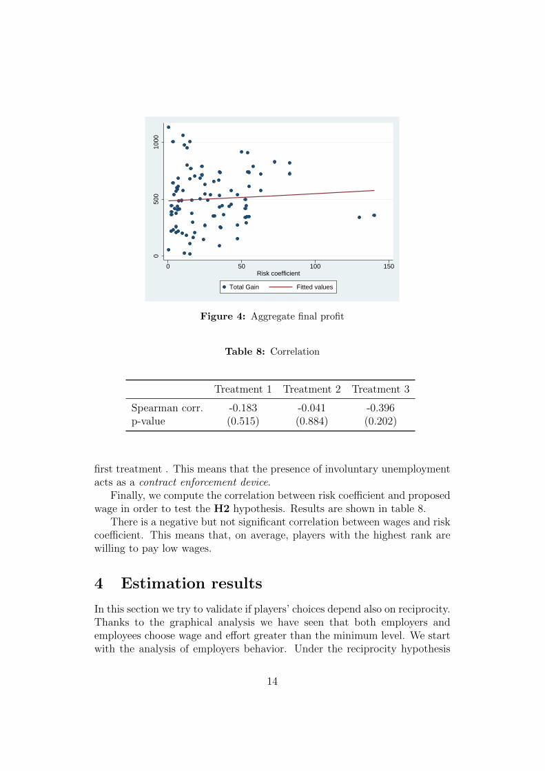
According to the value of this coefficient we assign a rank and playerswith the highest rank play in the role of employers. The amount of theinitial endowment is only useful for participation to this stage and does notinfluence the final profit of players5.

We test three hypotheses:

H1 Unemployment has a negative impact on wage formation. We expectthat in a context with high inequality workers are willing to accept anyoffer.6

H2 If employers are risk lovers then we expect them to offer low wages.This means that they are willing to accept the risk that a contractwith very low wages is not accepted.

H3 Players behave reciprocally, that is we expect to observe a positivecorrelation between wage and effort, regardless of the different unem-ployment rate.

We implement the standard BGE procedure. In the first stage employerssimultaneously propose a contract which contains wage and required effort(w, e) . In the second stage workers observe all the contracts and they canchoose only one offer. Workers who accepted a contract choose the real effort(e). The cost associated (c(e)) to any level of effort is shown in Table 1. Inour case, as in the Weak Reciprocity Treatment treatment in Fehr et al.(1997), if workers decide to shirk, a random mechanism determines whetherthe penalty f should be paid or not.

We consider a payoff function for employers that rules out losses, that is

πf = (v − w)e

in which v = 120 is the redemption value, e is the real effort chosen byemployees and the wage is such that

11 ≤ w ≤ 120

where the lower bound means that the minimum wage is greater than thesubsidy to unemployed, while the upper bound is a specification in order toavoid employers’ losses.

5Notice that we know the endowment earned thanks to the questionnaire and we haveall treatments with the same mean distribution of the endowment (µ1 = 100.33 , µ2 = 99.7and µ3 = 106.6). We check these values running an ANOVA and the result F = 0.32(p−value = 0.72) confirms that there are no significant differences in the distribution of theendowment.

6We fixed wmin > γ and so a rational worker has always an incentive to accept acontract even if the wage is the lowest.

5

Table 1: Cost function

e 0.1 0.2 0.3 0.4 0.5 0.6 0.7 0.8 0.9 1

c(e) 0 1 2 4 6 8 10 12 15 18

The expected payoff function of workers depends on the decision to shirk,that is:

πw =

w − c(e) if e ≥ e

(1− p)(w − c(e)) + p(w − c(e)− f) if e < e

The fine is a function of the difference between required and real effort.Workers know that the greater the difference, the greater the fine, but theyare able to see the penalty only after their choice.

The theoretical solution of standard Game Theory is based upon thehypothesis of perfect rationality. Under this hypothesis and using backwardinduction, the best strategy for the employee is to choose the minimum effortlevel, i.e. the level corresponding to zero cost. Employers, knowing the em-ployees choice, are willing to pay the minimum wage. The Nash Equilibriumfor the baseline game is given by the following strategies:

e∗ = min(e) = 1 for workers

w∗ = min(w) = 11 for firms

In our setting, as in the work by Fehr et al. (1997), if workers decide toshirk with a probability s = 0.3 they must pay a fine. The fine is increasingfunction of the difference in effort, that is

f = (e− e)(1.5) if e < e

According to this approach the best rational choice is to shirk if

f <c(e)− c(e)

s

6

Table 2: Descriptive statistics: wage

WageMean St.Dev Min Max Obs.

Treatment 1 67.63 27.20 20 119 398Treatment 2 38.63 25.46 12 113 404Treatment 3 46.26 28.24 11 110 360

in which c(e) is the cost related to the proposed effort and c(e) is thecost of the real effort. The difference between these costs is positive if e < eand we set f = 0 if e > e. This solution suggests that the best rationalchoice is to shirk if the fine is less than the difference in costs divided bythe probability to be controlled. We check that this condition holds for eachlevel of effort.

3 Experimental results: descriptive statistics

and graphical analysis

In this section we report the main results of the experiment. We analyzethe mean and the shape of wages and effort between treatment in order tovalidate our initial hypotheses. Moreover, we are interested in the analysisof agents’ behavior to test if they behave reciprocally.

We start our analysis with the observation of employers behavior. In Ta-ble 2 we report the main descriptive statistics of the proposed wage. Thehighest average wage was proposed in the control treatment, where at leastone employer proposed the highest possible wage. Contrary to our expecta-tion, the lowest mean is in the second treatment.

Figure 1 shows the average wage for each period. The horizontal line is theminimum wage, i.e. w = 11. It is easy to see tha in all treatments the meanwages are significantly higher than the minimum, i.e. the Nash equilibrium.In the second treatment, also in the first period the average wage is lowerthan that in other treatments. The wage gap between treatments becomeslarger during the first five periods.

This result confirms our hypothesis (H1), that a positive involuntary un-employment rate reduces the proposed wage. Indeed, treatment with thehighest unemployment rate is the only one that shows a decline over repe-

7

020

4060

8010

0W

age

0 5 10 15Period

Treatment 1 Treatment 2Treatment 3

Figure 1: Average wage by treatment

tition. We run a parametric and non parametric test to confirm graphicalresults and, as we can see in Table 3, both of them reject the null hypoth-esis (p − value in parenthesis). The difference in mean of the wage in theexperimental and control treatments is significant.

The main tool to analyze workers’ behavior is the analysis of the choseneffort. Table 4 reports the main descriptive statistics for this variable. Inthis case the highest mean is in the third treatment.

Employees choose the level of effort taking into account the related costsand the contract, i.e. wage and effort. As Table 4 shows, the highest meanis in the third treatment while the lowest is in the first. On the one hand,

Table 3: Statistics test : wage

Statistics test

Treatment 2 Treatment 3

t-test t= 15.040 t= 10.619(0.0000) (0.000)

Wilcoxon z= 13.991 z= 10.240(0.0000) (0.000)

8

Table 4: Descriptive statistics: Real effort

Real EffortMean St.Dev Min Max Obs.

Treatment 1 5.00 2.60 1 10 200Treatment 2 5.55 2.76 1 10 203Treatment 3 6.10 2.56 1 10 180

Table 5: Descriptive statistics: Proposed effort

Proposed EffortMean St.Dev Min Max Obs.

Treatment 1 5.695 0.16 5 6 200Treatment 2 7.20 0.13 6 7 203Treatment 3 6.95 0.15 6 7 180

9

Table 6: Statistics test: effort

Statistics test

Treatment 2 Treatment 3

t-test t= -2.98 t= -4.11(0.038) (0.000)

Wilcoxon z= -2.079 z= -3.910(0.0376) (0.0001)

according to the Shirking Theory, the higher the unemployment, the higher isthe workers’ willingness to exert more effort. On the other hand, accordingwith the reciprocity hypothesis, we expect to observe the highest averageeffort in the control treatment in response to the highest mean wage. It isinteresting to see also the average proposed effort which is shown in Table5. In the first and in the third treatments there is no significant differencebetween the desired and the real effort. In the second treatment the differencebetween these value is huge. Thanks to this comparison we should assertthat reciprocity plays an important role in the workers’ choice. Indeed, inthe second treatment the gap between proposed and real effort depends onthe low wage paid by employers.

We have shown that involuntary unemployment has a significant effecton the wage. We also test if there are significant differences among averagereal effort using t-test and Wilcoxon test. Results are shown in Table 6.

Both tests are not able to accept the null hypothesis. This means thatunemployment affects also the real effort. Unemployment has a negativeimpact on wage and a positive effect on effort. Employers are willing to paya lower wage in a market with high unemployment because employees arewilling to accept also a low offer. On the other hand, in a market with a highunemployment rate, workers choose a high level of effort and try to give apositive signal to their employers.

As we have already said, we want to analyze the relation between effortand wage to test if there is evidence for reciprocal behavior. We use rent as aproxy of employers’ reciprocity. Rent is the difference between the proposedwage and the minimum wage (r = w − wmin). As in Rabin (1993), play-ers behave reciprocally if they take into account the intentions signaled byopponents’ actions. In the field of labor market, we can say that employersbehave reciprocally if they are willing to pay a higher wage in response to

10

Table 7: Correlation

Treatment 1 Treatment 2 Treatment 3 Overall

Spearman corr. 0.204 0.130 0.236 0.119p-value (0.003) (0.05) (0.001) (0.004)

a high effort level and vice versa. According to this theory, we must checkif employees are willing to choose a high level of effort in response to a highwage. We consider the Spearman correlation, that is a non parametric testin which the null hypothesis is the independence of variables. The correla-tion between wage and effort is shown in Table 7. In all treatments thereis a positive and significant correlation. This result confirms our startinghypothesis. We test this conjecture with a regression hereafter.

We can assert that in our setting there is a “gift exchange” betweenemployers who always offer a wage such that w > w and employees thatguarantee a positive effort, i.e. e > emin. The main difference between thegift exchange and the reciprocity approach is that in the former workers arewilling to choose greater real effort than that in the contract. In our analysisthere is a positive correlation between rent and wage, but only 9% of workerschoose a level of effort greater than the proposed one. Hereafter we analyzethis relation using OLS estimation.

As we have already said, we fix the minimum wage so that rational workersalways have an incentive to accept a contract. In the previous section we haveseen that according to the standard Game Theory the best rational choicefor employees is to shirk despite the fact that they should pay a fine. InFigure 2, we show the percentage of shirking in each treatment. We identifythe shirking behavior as a dummy variable that is equal to 1 if e < e and 0otherwise.

It is easy to see that the second treatment registers the highest percentageof shirking, i.e. 50%, while in the other two treatments the percentage isabout 30%. The high percentage of shirking in the second treatment isuseful to explain why the mean wage is the lowest. Indeed, employers areable to observe unkind employees’ behavior and, as a consequence, they arewilling to offer a low wage. In turn, employees who receive low wages punishtheir employers by choosing a low level of effort. According to this theory,a high involuntary unemployment rate is a deterrent for shirking. In thefirst treatment there is no excess of labor supply, so employees are willing torespect the contract to reciprocate the high wage paid by employers. This

11

0.2

.4.6

.80

.2.4

.6.8

-1 0 1 2

-1 0 1 2

Treatment 1 Treatment 2

Treatment 3Den

sity

ShirkingGraphs by treatment

Figure 2: Percentage of Shirking

means that, in this case, positive reciprocity plays a crucial role. Finally,it is interesting to analyze the shape of unemployment. In our setting weconsider involuntary and voluntary unemployment, that is we give employeesthe possibility of accepting no contract if the proposed wage is lower thantheir reservation wage. In Figure 3 we show the unemployment rate in eachperiod and we add, as a reference point, the initial unemployment rate. Itis interesting to highlight that in treatment 1 there is a high unemploymentrate and that this is only voluntary.

This means that workers are willing to not accept offers in order to signaltheir reservation wage. Also in the second treatment there is voluntary un-employment but this is joined with high shirking rate. In the last treatmentthere is no voluntary unemployment because the induced rate is very highand workers are willing to accept any offer.

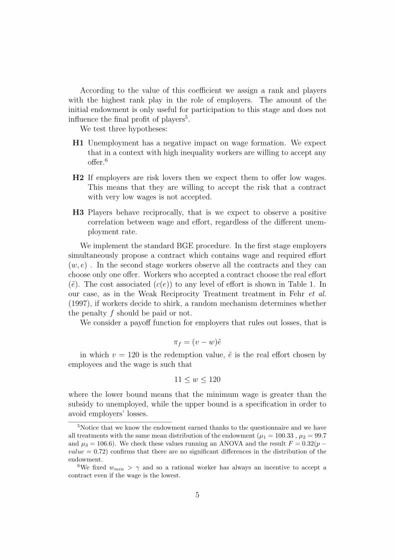
Finally, we want to analyze the impact of risk aversion. As we havesaid, we assign to the role of employers those who show the highest riskcoefficient, that is a linear combination of the initial endowment and theinvestment in the lottery. We consider this combination in order to takeinto account both the smartness and the propensity to risk. In Figure 4,we show the relation between the total profit, that is the cumulative gainsduring the game, and the risk coefficient. In this graph we consider both theemployees and employers gains. As we can see, the relation between thesevariables is positive. This is also confirmed by the Spearman correlation test(ρ = 0.19, p − value = 0.06) . This suggests that, on average, employers’

12

0.1

.2.3

0.1

.2.3

0 5 10 15

0 5 10 15

Treatment 1 Treatment 2

Treatment 3

unemployment rate unemployment (t0)

Period

Graphs by treatment

Figure 3: Unemployment rate

profits are greater than employees’ ones.Remember that payoff functions are such that:

∂πf∂w

< 0∂πf∂e

> 0

∂πe∂w

> 0∂πe∂e

< 0

In Figure 5 we see the average payoff per period of employers and em-ployees divided by treatment. The first treatment is the only one in whichthe profit share is lower than the wage share. This is the result of two mainaspects that we have already analyzed. The first treatment is that with thehighest mean wage and, at the same time, the lowest mean effort. Thismeans that with no exogenous excess of labor supply, workers use voluntaryunemployment as a tool to increase their bargaining power. The result isthat in this treatment the wage share is always greater than the profit share.In the second and third treatment profits are greater than wage. The pres-ence of involuntary unemployment reduces the employees’ bargaining power.According with the Shirking Theory of Shapiro and Stiglitz (1984), an excessof labor supply is an incentive for workers to exert a high level of effort. Thisis true especially in the third treatment in which there is an unemploymentrate of 20%. Remember that in this treatment the level of effort is the high-est. Moreover, in this treatment wages are, on average, less than those in the

13

050

010

00

0 50 100 150Risk coefficient

Total Gain Fitted values

Figure 4: Aggregate final profit

Table 8: Correlation

Treatment 1 Treatment 2 Treatment 3

Spearman corr. -0.183 -0.041 -0.396p-value (0.515) (0.884) (0.202)

first treatment . This means that the presence of involuntary unemploymentacts as a contract enforcement device.

Finally, we compute the correlation between risk coefficient and proposedwage in order to test the H2 hypothesis. Results are shown in table 8.

There is a negative but not significant correlation between wages and riskcoefficient. This means that, on average, players with the highest rank arewilling to pay low wages.

4 Estimation results

In this section we try to validate if players’ choices depend also on reciprocity.Thanks to the graphical analysis we have seen that both employers andemployees choose wage and effort greater than the minimum level. We startwith the analysis of employers behavior. Under the reciprocity hypothesis

14

050

100

150

200

050

100

150

200

0 5 10 15

0 5 10 15

Treatment 1 Treatment 2

Treatment 3

Payoff employers Payoff employees

Period

Figure 5: Wage share and Profit share

employers are willing to pay a higher wage if employees choose a positiveeffort. We run the following estimation

rit = α + β0eit + β1sit + β2ut + β3δi + εit, (1)

where rit7 is the proposed rent, eit is the real effort, sit is a dummy

variable for shirking equal to 1 if the worker chooses to shirk, ut is theexcess of labor supply and δi is the risk coefficient and εit = vt + µit is theerror component which includes also individual specific characteristics. Byestimating this equation we test the impact of both employees’ behavior andthe unemployment rate on rent.

We consider a panel regression with Random Effects. We choose RandomEffects instead of Fixed Effects specification because we are interesting inestimating the impact of the risk coefficient on the proposed effort and thiscoefficient is time invariant.8

The main results are shown in Table 9. Real effort has a positive andsignificant effect on the rent. The shirking dummy has a negative and sig-nificant impact: if employees shirk, employers offer a low wage in the next

7The subscript i is for individual observation and the subscriptt is the time seriesdimension.

8We consider robust standard errors and we test for the serial correlation using theWooldridge test. The test accepts the null hypothesis of absence of auto correlation (F =0.005, p − value=0.943 , F = 0.012, p − value = 0.912 are the statistics relative to firstand second estimations, respectively).

15

Table 9: RE estimation of the rent equation

(1)Rentβ (SE)

Real Effort 1.883***(0.480)

Shirking -8.509***(2.554)

Unemployed -4.128***(0.765)

Risk Coefficient -0.010(0.194)

Constant 49.285***(4.757)

Observations 542R-overall 0.161

Dependent Variable: Rent

period. This means that employees’ behavior strongly influences the employ-ers’ willingness to pay high rent. The number of the unemployed has also anegative impact while the risk coefficient has no significant impact on rent.This means that rents are strongly influenced by the “market condition”,especially by the number of voluntary unemployed in each period.

Regarding the employees’ behavior we want to analyze if real effort isinfluenced by the proposed contract. As we have already seen in the graphicalanalysis, the highest percentage of shirking is in the second treatment andthat the mean wage in the second treatment is the lowest. Taking intoaccount this information, the high percentage of shirking can be seen asnegative reciprocity. Employees prefer to accept low wages rather than beunemployed, but they consider low wages as an unfair offer. Their responseto unkind behavior is to accept a contract but choose a lower level of effortthan the required one.

In order to test the reciprocity hypothesis we estimate the following effortequation:

eit = α + β0wit + β1eit + β2uit−1 + εit,

16

where the dependent variable is the real effort, wit is the wage of eachperiod, eit is the desired effort and ui is a dummy variable which is equalto one if the worker was unemployed in the previous period. We consider apanel estimation with Fixed Effect specification with robust standard errors.9 Table 10 shows the result of our regression. The first and the secondvariables measure the impact of the contract conditions on the real effort.Both coefficients are positive and significant. It is interesting to highlightthat the wage has a lower marginal effect than the proposed effort. Thismeans that employees care about the request of their employer and theirchoices are less sensitive to changes in wage. In the previous section weshow that workers always have an incentive to choose the lowest effort, i.ee = 1. So, the strong impact of the proposed effort on the real choice canbe explained as an anchoring effect. This means that their choice is stronglyinfluenced by the number of hours that employers propose. We consider alsothe worker’s condition in the previous period. As we can see, this variablehas a positive and significant coefficient. This means that if worker did notsubscribe any contract in the previous period then she/he is willing to choosea higher effort in the next period. A possible explanation is related to theidea that workers try to construct a sort of reputation choosing a high levelof effort in order to avoid being unemployed in the next period.

Finally, we are interested in understanding the determinants of the proba-bility of no-shirking. As we have seen, real effort is influenced by the contract,i.e. the wage and proposed effort. We run the following Probit estimationwith Random Effects:

Prob(ϑit = 1|X) = α + β0wit + β1fit−1 + β2u+ β3wit−1 + εit

ϑ is the probability of non shirking, i.e. ϑ = 1 if worker does not shirk. wit

is the wage, fit−1 is a dummy variable equal to 1 if the employee paid a finein the previous period. This dummy is a measure of the level of monitoring.u is the exogenous excess of labor supply, wit−1 is the wage in the previousperiod.

The analysis of the probability of no shirking is useful to evaluate theassumption of Shirking Theory. Our starting hypothesis is that both em-ployers and employees make their choice taking into account the strategy oftheir opponent, that is they behave reciprocally. Under the assumption ofthe Shirking Theory we should observe that employees behavior is influencednot only by the wage but also by involuntary unemployment and the level of

9We check the absence of autocorrelation. The test accepts the null hypothesis(F=0.621, p−value =0.435). We estimate also the model with Random Effect and we usethe Hausman test. The test rejects the null hypothesis (χ2 = 11.891, p− value = 0.007).

17

Table 10: FE estimation of the effort equation

(1)Real Effortβ (SE)

Wage 0.017***(0.003)

Required Effort 0.577 ***(0.041)

Unemployedt−1 0.308 **(0.124)

Constant 0.606(0.390)

Observations 525R-overall 0.235

Dependent Variable: Real effort

Table 11: Output Regression: Probability of no-shirking

ϑβ (SE)

Waget 0.023***(0.005)

Waget−1 -0.005(0.005)

Finet−1 -0.013(0.017)

Unemployment rate 4.696*(2.466)

Constant -1.492***(0.534)

Observations 185

Dependent Variable: Probability of no-shirking

18

monitoring. Output regression is shown in Table 11. It is easy to see thatthe only significant coefficient in the Probit regression is the wage. In partic-ular, the higher the wages paid by employers, the higher the probability ofno shirking. All the other coefficients are not significant. Unemployment hasa positive coefficient as we expect. In fact, workers try to behave “correctly”in order to decrease the probability of being unemployed. Involuntary unem-ployment affects the chosen effort but only the wage has a significant effecton employees behavior. This result confirms that employees and employersare mainly driven by the behavior of their counterpart.

5 Conclusion and future analysis

In this chapter we analyzed the dynamic in the job market using experimentalevidence. We are interested in the study of the impact of unemployment onthe wage and on the behavior of both employers and employees. We use theGift Exchange Game in order to test our hypothesis. The main novelty thatwe introduce with respect to the literature is the assignment of players intheir role according to a measure of risk aversion. We assigned participantswith the higher risk aversion to the role of workers. We consider a one shotgame with 15 repetitions. Our results show that involuntary unemploymenthas a negative impact on wages, that is, in absence of unemployment weobserved the highest mean wage. Moreover, we observed a high voluntaryunemployment rate only in the control treatment.

Unemployment has a negative effect on the trust relation between thetwo parties. According to the Shirking Theory, an excess of labor effort isan effective device to incentive workers to exert a higher level of effort. Inthe third treatment, in which the unemployment rate is equal to 20%, resultsare in line with the theoretical predictions. Indeed, the wage is greater thanthe lower bound and the percentage of shirking is very low. In the othertreatment there are very different results. In the treatment in which theunemployment rate is equal to 12%, there is evidence for negative reciprocity.The result of this behavior is a very low mean wage and very high percentageof workers who decide to shirk.

Finally, we showed that the the level of monitoring, measured with theprobability of paying a fine, has no significant impact on the probability ofshirking. This implies that paying a higher wage, or in general offering agood contract, has a greater impact on the kind behavior of the employeerather than increasing the level of monitoring.

Currently in our country, as in the other OECD countries, we observe avery high unemployment rate. This is particularly true if we consider youth

19

unemployment rate. In Italy we have reached the peak of 43% in the firstquarter of 2014. According to the Neoclassical theory, firms should cut wagesin order to hire more workers. We have shown, using a very simplified envi-ronment, that the labor market does not work as other markets, that is wagesdo not follow the best demand-supply rule. In contrast, our results show thatworkers are willing to reciprocate employers behavior both in positive andnegative way. If employers are willing to pay very low wages, employees ac-cept a contract because of the very high unemployment rate, but they arewilling to reciprocate choosing to shirk. This means that cutting wages re-sults in a reduction in the labor productivity which, in turn, should reducealso firms’ profit.

In our opinion, the main tool to reduce unemployment is to propose ashort-term contract with “kind conditions”, that is paying high wages. Theshort-term condition is favorable for firms which should increase or decreaselabor demand according to the real demand for goods and services. Bothemployers and employees would benefit from the “kindness” condition. Onthe one hand, high wages improve the workers’ standard of living and actas an incentive to increase productivity. On the other hand, high wagesare costly for firms but are able to increase productivity per employers andso the final profit. It is important to remark that the flexibility in the jobmarket should be associated with a good welfare system to safeguard workers’position.

Our aim is to investigate with further experimental analysis the impactof reciprocity, using a setting in which a firm hires more than one worker.The focus of this kind of experiment is to test if the reciprocity motive is asstrong in multi-players interaction as in the two players context.

20

References

Ackerlof, G. A. (1982). Labor contracts as a partial gift exchange. TheQuarterly Journal of Economics, 42, 543–569.

Brown, M., Falk, A., and Fehr, E. (2004). Relational contracts and the natureof market interactions. Econometrica, 72(3), 747–780.

Campbell, C. and Kamlani, K. (1997). The reasons foe wage rigidity: Evi-dence from survey of firms. Quarterly Journal of Economics, 112, 759–789.

Casoria, F. and Riedl, A. (2013). Experimental labor markets and policyconsiderations: Incomplete contracts and macroeconomic aspects. Journalof Economic Surveys, 27(3), 398–420.

Charness, G. (2004). Attribution and reciprocity in an experimental labormarket. Journal of Labor Economics, 22(3), 665–688.

Fahr, R. and Irlenbusch, B. (2000). Fairness as a constraint on trust inreciprocity: earned property rights in a reciprocal exchange experiment.Economics Letters, 66(3), 275–282.

Falk, A. (2007). Notes and comments gift exchange in the field. Econometrica,75(5), 1501–1511.

Falk, A. and Fischbacher, U. (2006). A theory of reciprocity. Games andEconomic Behavior, 54(2).

Fehr, E. and Falk, A. (1999). Wage rigidity in a competitive incompletecontract market. The Journal of Political Economy, 107(1), 106–134.

Fehr, E. and Falk, A. (2008). Reciprocity in experimental markets. Handbookof Experimental Economics Results, 1, 325–334.

Fehr, E. and Gatcher, S. (2000). Fairness and retaliation: The economics ofreciprocity. Journal of Economic Perspective, 14(3), 159–181.

Fehr, E., Kirchsteiger, G., and Riedl, A. (1993). Does fairness prevent marketclearing? an experimental investigation. quarterly Journal of Economics,108, 437–459.

Fehr, E., Kirchsteiger, G., and Riedl, A. (1996). Involuntary unemploymentand non-compensating wage differentials in an experimental labour market.The Economic Journal, 106(434), 106–121.

21

Fehr, E., Gatcher, S., and Kirchsteiger, G. (1997). Reciprocity as a contractenforcement device: experimental evidence. Econometrica, 65(4), 833–860.

Fehr, E., Kirchler, E., Weichbold, A., and Gachter, S. (1998). When socialnorms overpower competition: gift exchange in experimental labor market.Journal of Labor Economics, 16(2), 324–351.

Fischbacher, U. (2007). z-tree: Zurich toolbox for ready-made economicexperiments. Experimental Economics, 10(2).

Gneezy, U. and List, J. A. (2006). Putting behvioral economics to work:testing for gift exchange in labor markets using field experiment. Econo-metrica, 74(5), 1365–1384.

Pereira, P. T., Silva, N., and e Silva, J. A. (2006). Positive and negative reci-procity in the labor market. Journal of Economic Behavior and Orgniza-tion, 59, 406–422.

Rabin, M. (1993). Incorporating fairness into game theory and economics.American Economic Review, 83.

Shapiro, C. and Stiglitz, J. E. (1984). Equilibrium unemployment as a workerdiscipline device. The American Economic Review, 74(3), 433–444.

22

A Experiments using z-tree: Gift Exchange

Game

In this section we show the screen shoots of the second experiment, that isthe Gift Exchange Game. The general instructions are read aloud before thebeginning of the game. In this experiment the allocation of players is notin a random order but we assign a seat according to the initial endowment.Remember that players earn the initial endowment according to the numberof right answers about logic and general culture.

Before starting, players use their own endowment to play in a lottery.They read the instructions to participate and then they enter the amountthey are willing to bet, as shown in Figure 6. Thanks to this choice we areable to assign each player in the role of employer or employee.

At the beginning of the game players read on their own screen the specificinstruction for their type. A summary is reported in Figures 7 and 8.

Figure 9 shows the next step. Players in the role of employers maketheir offer. they must insert the wage and the proposed effort. We imposethe upper and lower bounds for both variables in order to respect the limits11 ≤ w ≤ 120 and 1 ≤ e ≤ 10.

After all the employers have made their offer, players in the role of em-ployees choose one of the feasible contracts. As in Figure 10, each employershould select one of the contracts or simply press the button CONTINUAand accept no contract. Each employer has a number in order to avoid theexact identification of the proposer.

Employees who have subscribed a contract must choose the level of effort.As shown in Figure 11, we pick a bullet in correspondence of the requiredeffort. They should choose any level between 1 and 10 taking into accountthe cost function in their screen.

Thanks to the real effort we are able to calculate the profit for employersand employees. In the final screen, in each period they see only their personalpayoff.

Table 12 shows the descriptive statistics of the final payment in eachtreatment. In the first treatment we register the higher average final profit. InTable 13 we can see that employers’ final profit is higher than employees’one.

23

Figure 6: Lottery

24

Figure 7: Instructions for employees

25

Figure 8: Instructions for employers

26

Figure 9: Contract

27

Figure 10: List of contracts

28

Figure 11: Real effort choice

29

Table 12: Descriptive statistics: Final payment

PaymentMean St.Dev Min Max

Treatment 1 13 0.89 11 14Treatment 2 11.78 0.77 10 13Treatment 3 10.1 0.82 8 11

Table 13: Descriptive statistics: Final payment by type

PaymentMean St.Dev Min Max

Type 1 12.83 0.63 11 14Type 2 10.64 0.70 9 12

30