Document Title: Labor Force Participation, Labor Markets, and Crime
Upload
khangminh22Category
view
7download
0
1
98707
T h e I m p a c t o f T a r g e t e d S o c i a l A s s i s t a n c e o n
L a b o r M a r k e t i n G e o r g i a 1
A R e g r e s s i o n D i s c o n t i n u i t y A p p r o a c h
May 2015
SOCIAL PROTECTION AND LABOR GLOBAL PRACT ICE
World Bank
Document of the World Bank
1 This report was prepared by Barbara Kits, Indhira Santos, Aylin Isik-Dikmelik and Owen Smith as part of task no.
EW-P128205-ESW-TF010804. The task is financed by the Trust Fund for Environmentally and Socially Sustainable
Development (TFESSD). The Task Team Leader (TTL) is Indhira Santos.
Pub
lic D
iscl
osur
e A
utho
rized
Pub
lic D
iscl
osur
e A
utho
rized
Pub
lic D
iscl
osur
e A
utho
rized
Pub
lic D
iscl
osur
e A
utho
rized

2
CURRENCY EQUIVALENTS
(Exchange Rate Effective: September, 2014)
Currency Unit = Georgian Lari (GEL)
1 GEL = 0.57465 US$
1 US$ = 1.74020 GEL
ECA Regional Vice President:
Social Protection and Labor Senior Director:
Laura Tuck
Arup Banerji
Practice Manager: Andrew Mason
Task Team Leader:
Authors:
Indhira Santos
Barbara Kits, Indhira Santos, Aylin Isik-
Dikmelik, Owen Smith

3
TABLE OF CONTENTS
Currency Equivalents .................................................................................................................................... 2
Table of Contents .......................................................................................................................................... 3
List of Figures ............................................................................................................................................... 4
List of Tables ................................................................................................................................................. 4
List of Boxes ................................................................................................................................................. 4
List of Acronyms ........................................................................................................................................... 5
Executive summary ....................................................................................................................................... 6
Acknowledgements ....................................................................................................................................... 7
1. Introduction ............................................................................................................................................... 8
2. Background ............................................................................................................................................. 10
2.1 Review of Existing Literature ........................................................................................................... 10
2.2 Georgia’s ‘Targeted Social Assistance’ Program .............................................................................. 12
2.2.1. An Overview of Social Protection in Georgia ........................................................................... 12
2.2.2. The TSA Program...................................................................................................................... 13
2.2.3. Evaluation of TSA: Satisfaction with Program Implementation and Effectiveness .................. 16
3. Sampling Frame, Sampling and Data ...................................................................................................... 19
3.1 Sampling Frame and Sampling ......................................................................................................... 19
3.2 The Data ............................................................................................................................................ 21
4. Empirical Approach ................................................................................................................................ 23
5. Main Results ............................................................................................................................................ 28
6. Conclusion ............................................................................................................................................... 35
References ................................................................................................................................................... 37
Annex 1: Regional Sample Composition ................................................................................................ 39
Annex 2: Reasons for Non-Response ...................................................................................................... 39
Annex 3: Descriptive Statistics ............................................................................................................... 40
Annex 4: Labor Force Participation by Score Group .............................................................................. 42
Annex 5: Mean Values of Covariates – Labor Force Participation ......................................................... 44
Annex 6: Labor Force Participation RDD Results .................................................................................. 46

4
LIST OF FIGURES
Figure 1: Who Would Start Looking for Work if the Household Lost 20 Percent of its Income? ................ 9
Figure 2: Social Protection Spending in ECA (Percent of GDP): Latest Year Available ........................... 12
Figure 3: Social Protection Expenditure (Percent of total), 2012 ................................................................ 13
Figure 4: Indicators Included in Composite PMT Welfare Score ............................................................... 14
Figure 5: Schematic Overview of PMT Score-groups ................................................................................ 14
Figure 6: TSA – Coverage, Targeting Accuracy and Generosity, 2011 ...................................................... 15
Figure 7: Government Expenditure on TSA, 2008-2013 ............................................................................ 16
Figure 8: Share of Respondents Evaluating the Application Process as ‘Unfair’ ....................................... 17
Figure 12: TSA Evaluation by Recipient Households................................................................................. 17
Figure 10: Sampling Frame: Densities around the Cutoff Score ................................................................. 20
Figure 11: History of Receiving TSA ......................................................................................................... 23
Figure 12: Score Distributions in the Sample .............................................................................................. 25
Figure 13: Switching Patterns over Time: Share of Households in TSA Sample ‘Switching’ Treatment
Status, by the Timing of their Latest Scoring Event.................................................................................... 27
Figure 14: Labor Force Participation in the TSA Sample ........................................................................... 28
Figure 15: Conditional Effect of Receiving TSA on Labor Force Participation: Summary of Model
Specifications .............................................................................................................................................. 29
Figure 16: Predicted Labor Force Participation, by Gender ........................................................................ 29
Figure 17: Labor Force Participation Rates for Working Age Women, by Family Status.......................... 31
Figure 18: Share of Working Age Respondents Expressing Agreement with the Statement: “I would enjoy
having a paid job even if I did not need the money” ................................................................................... 32
Figure 19: Labor Market Preferences: Inactive Women and Women in the Labor Force, Working Age (15-
59) ................................................................................................................................................................ 32
Figure 20: Reservation Wages among Treatment and Control Group ........................................................ 34
LIST OF TABLES
Table 1: Recent Changes in TSA Program Design, 2009-2013 .................................................................. 16
Table 2: Share of Subjects Expressing Agreement with Various Statements on Social Benefits in Georgia
..................................................................................................................................................................... 18
Table 3: Sample Composition ..................................................................................................................... 21
Table 4: Basic Characteristics of the SAHI Sample Compared to Georgian Population ............................ 22
Table 5: Income & Assets in the SAHI Sample, by Urban / Rural Location .............................................. 22
Table 6: Conditional Effect of Receiving TSA on Labor Force Participation: Summary of Model
Specifications for Various Groups of Women ............................................................................................ 30
Table 7: Self-reported Attitudes on Work, Family Responsibilities and Gender: Share of Working Age
Respondents (15-59 for women, 15-64 for men) Expressing Agreement with each Statement .................. 33
Table 8: Conditional Effect of Receiving TSA on Labor Force Participation: Summary of Model
Specifications for Urban/ Rural Sample ...................................................................................................... 34
LIST OF BOXES
Box 1: Georgia’s Means-Testing Methodology .......................................................................................... 14

5
LIST OF ACRONYMS
ECA Europe and Central Asia
GDP Gross Domestic Product
GEL Georgian Lari
HBS Household Budget Survey
IDP Internally Displaced Person
LATE Local Average Treatment Effect
LiTS Life in Transition Survey
LMMD Labor Market Micro-level Database
MIP Medical Insurance for the Poor
MoHLSA Ministry of Health, Labor and Social Affairs
PER Public Expenditure Review
PMT Proxy Means Test
RDD Regression Discontinuity Design
SAHI Survey Social Assistance and Health Insurance Survey
SPeeD Social Protection expenditure & evaluation Database
SSA Social Services Agency
TFESSD Trust Fund for Environmentally and Socially Sustainable Development
TSA Targeted Social Assistance
UDSUF United Database for Socially Unprotected Families
UNECE United Nations Economic Commission for Europe
UNICEF United Nations International Children’s Emergency Fund
USAID United States Agency for International Development
USD US Dollar
WMS Welfare Measurement Survey
6
EXECUTIVE SUMMARY
This report examines the impact of social assistance programs on labor force participation in the Republic
of Georgia. In particular, it evaluates the ‘Targeted Social Assistance’ (TSA) program, which provides a
monthly subsidy to families below a welfare threshold.
Social assistance programs have a key role to play in protecting households from shocks, ensuring a
minimum level of subsistence and facilitating efficient labor market transitions. However, these programs
could also unintentionally reduce incentives to work, especially in the formal sector if the income effect is
sufficiently large, their design disproportionally taxes work and/or eligibility criteria explicitly or
implicitly make working (formally) less attractive. Few rigorous studies exist that establish the causal link
between social assistance and labor market outcomes in developing countries.
In the case of Georgia, applicant households are evaluated through a proxy means test to determine
eligibility for the TSA program. For this study, a newly designed survey of approximately 2000
households and administrative data were combined with a regression discontinuity design in order to
exploit the sharp discontinuities in treatment – defined as being a beneficiary of TSA – around the proxy
means score threshold.
Results suggest that the TSA program indeed generates work disincentives around the eligibility
threshold, with these disincentives concentrated among women. On average, women who receive TSA are
7 to 11 percentage points less likely to be economically active than women who live in households that do
not receive the transfer. This is a very large effect given that the labor participation rate among women in
the sample is 60.5 percent. Moreover, the analysis indicates that disincentives effects are larger for
younger women, and for women who are married and/or have children. Among men, there is no
statistically significant effect. These findings are supported by various robustness and falsification tests.
These findings have important policy implications. First, they highlight the importance of carefully
considering potential work disincentive effects of further increases in the generosity of the TSA program,
and the potential benefits of considering an expansion of coverage rather than an increase in generosity. A
comparable evaluation of the TSA program in 2007 found no work disincentive effects, but the program
then was only half as generous as it is today. Second, this report suggests that strengthening the provision
of complementary services, such as child and elderly care, can go a long way in reducing the TSA work
disincentive effects found among women, since the women that stop working (formally) are young, have
young children or are married. In addition, the evidence on potential and reservation wages suggests that
improving the access to training and upskilling of women in rural areas can be an important part of the
agenda for getting them into work outside of their homes. Finally, the report also points at the potential
benefits of combining the social assistance program with more stringent requirements to participate in job
search or activation programs, or to make receipt of benefits conditional on training requirements, for
either the children in the household, or in the form of life-long-learning, for inactive individuals of
working age. Furthermore, these results may be of value to other countries, if they have similar levels of
welfare and have adopted, or are planning to adopt, similar social assistance programs.

7
ACKNOWLEDGEMENTS
This work has been financed by the Trust Fund for Environmentally and Socially Sustainable
Development (TFESSD).
This report was started under the direction of Ana Revenga (previous Sector Director, Human
Development) and Alberto Rodriguez (previous Acting Sector Director, Human Development).
Supervision has been provided by Roberta Gatti (former Sector Manager and Lead Economist), Omar
Arias (former Acting Sector Manager) and Andrew Mason (Practice Manager, Social Protection and
Labor Global Practice).
This report was written by Barbara Kits, Indhira Santos, Aylin Isik-Dikmelik and Owen Smith. The team
is thankful to participants in the World Bank Poverty and Labor seminar in 2014 where very useful
comments were received. In addition, the report also reflects the work and efforts of other colleagues at
the World Bank. We are especially thankful to Robin Audy, Tomas Damerau, Joost de Laat and Ramya
Sundaram. David Newhouse acted as peer reviewer. For valuable comments to the design of the survey
used for this study, as well as for the implementation of this survey, we are thankful to the Georgian firm
Gorbi, headed by Merab Pachulia (Managing Director). This work also reflects analytical contributions
and policy expertise on issues of labor market inequality by other international institutions. Lastly, this
report reflects interactions with policy-makers and academics in Georgia.
This report is part of a larger package of analytical work, which also includes: 1) a general report on
inequalities in labor market participation, covering ten countries in Europe and Central Asia; 2) two other
case studies on Georgia and Tajikistan; and 3) a series of 9 country-reports based on qualitative research2,
including focus group discussions. The qualitative analysis was financed through country-specific as well
as regional World Bank projects, and implemented jointly with María Dávalos, Giorgia Demarchi and
Patti Petesch.
2 The following countries are included in this qualitative work: Bosnia and Herzegovina, Kosovo, Macedonia,
Serbia, Georgia, Turkey, Kazakhstan, the Kyrgyz Republic and Tajikistan.

8
1. INTRODUCTION
Since the transition, Georgia has had poor labor market outcomes, especially among women, youth
and older workers. One quarter of all households does not have a single employed individual.3 Only 55
percent of the adult population aged 15 and over is employed, a decrease from 59 percent in 2001.4 This is
substantially lower than in the best performing European countries. The low employment rate is primarily
driven by a high prevalence of unemployment, which stands at 14 percent. Labor force participation, at 64
percent of the adult population, is not exceptionally low overall, but this masks large inequalities between
various socio-economic groups.5 For example, inactivity is much higher among women than among men
(the difference in participation rates stands at 14 percentage points)6, and among youth, aged 15-24, as
compared to prime age workers. Almost one fifth (19 percent) of youth are not in employment, nor
enrolled in formal education or training, and about three quarters of these are out of the labor force.
Similarly, participation is lower among older workers (aged 55-64), and older women in particular often
exit the labor force early.
Those who do work often do so in low-productivity, low-paying jobs. For example, the agricultural
sector accounts for about half of total employment, and often does not offer a high or steady income year-
round.7 Especially among working women, the agricultural sector dominates – it accounts for 57 percent
of female employment.8 Moreover, 38 percent of working women and 20 percent of working men are
family workers, mostly unpaid, and 51 percent of working women (compared to 37 percent of working
men) work part-time rather than fulltime.9
Social assistance programs can help improve labor market engagement – through, for example,
improved household income and protection against shocks. However, such public programs can also
create disincentives to work – for instance, by introducing a loss of social assistance income as soon as
individuals start working. Hence, social assistance, though meant to support poor and vulnerable
households, could also have unintended adverse impacts.
This report examines the impact of a large social assistance program in Georgia, ‘Targeted Social
Assistance’ (TSA), on labor market outcomes. The TSA program provides a monthly subsidy to poor
families below a welfare threshold, identified through a proxy-means test. Although any household in
Georgia can apply for TSA, only those with low proxy-means test scores – representing low levels of
wealth – are granted benefits. The amount transferred to a family depends on the number of household
members, and consists of a base benefit (60 GEL currently; 30 GEL at the time of data collection) and a
top-up benefit per additional household member beyond the head of the household (48 GEL currently, 24
GEL at the time of data collection).
Studying Georgia’s TSA program is relevant for a number of reasons. First, the TSA program has a
good coverage of the poor when compared to other countries in Europe and Central Asia (ECA), and is
well-targeted. Second, recent changes in generosity allow for insights into the links between generosity
3 HBS, 2009.
4 World Bank, World Development Indicators.
5 World Bank, World Development Indicators.
6 HBS, 2009.
7 Rutkowski, 2012.
8 World Bank, World Development Indicators.
9 World Bank, World Development Indicators.

9
and work disincentives, as the results obtained here can be compared with an evaluation conducted in
2007, when the TSA program was less generous than it is now. In this previous study, no disincentive
effects were found. Third, as mentioned above, Georgia is a country where labor market outcomes remain
poor, and where understanding the complex reasons behind low participation or high unemployment for
different sub-population groups is of utmost importance. Finally, the design of the TSA program makes it
amenable to quasi-experimental evaluation, an opportunity to generate rigorous evidence on the impacts
of social assistance on work incentives.
There is reason to believe that Georgia’s TSA program may be generating disincentives to work.
When asked whether a negative income shock would make one or more household members to start
looking for work, about half of all TSA recipients sampled for this study responds positively.10
Among
non-recipients that are close to the eligibility threshold, responses are similar at 49 percent. Among TSA
beneficiaries, 17 percent of households responding positively to this question state that one or more
women, but no men, in the household would start looking for jobs; 27 percent state that one or more men,
but no women, would start looking for jobs, and 56 percent of households state that both men and women
would look for jobs in this scenario (Figure 1). Even when asked directly whether at least one household
member would stop working if the household would start receiving TSA, 6 percent of TSA non-recipient
households responds positively.
FIGURE 1: WHO WOULD START LOOKING FOR WORK IF THE HOUSEHOLD LOST 20 PERCENT OF ITS
INCOME?
TSA RECIPIENT HOUSEHOLDS WHO INDICATE THAT AT LEAST ONE INDIVIDUAL WOULD SEARCH
FOR WORK (%)
Source: Authors’ calculations, based on SAHI Survey, 2012-2013.
Notes: Sample restricted to households receiving TSA, who state that at least one person would start looking for work if the
household lost 20 percent of its monthly income.
This report uses of a regression discontinuity design, a new household survey and administrative
data to identify the causal effect of the TSA program on labor force participation in Georgia. Due to
its design features, the TSA program provides a unique opportunity to apply a regression discontinuity
analysis to measure the causal impact of social assistance on labor market outcomes by only focusing on
households of very similar socio-economic status.
10
When asked: “Would currently jobless household members start working / try to find work if the household lost
20% of its monthly income”, 48 percent of TSA recipient households states that this would indeed be the case. 20
percent is the typical share that TSA benefits represent of household income in Georgia.
14
3
22
5 35
6
9
6 0 men and 1 woman
0 men and 2 or more women
1 man and 0 women
2 or more men and 0 woman
1 man and 1 woman
1 man and 2 or more women
2 or more men and 1 woman
2 or more men and 2 or more women

10
This report contributes not only to the existing literature, but also provides suggestions for future
policy-design related to the TSA program in Georgia. First, our findings contribute to the existing
literature in two main ways: (i) we investigate, in a rigorous manner, the causal link between social
assistance and labor force participation in the context of a developing country, where relatively little
rigorous evidence exists; and (ii) we disentangle some of the potential channels through which the effects
found may come about, by quantifying the impacts of the program among different demographic,
educational and socio-economic groups. Second, the findings presented here can inform future policy
design in Georgia regarding the TSA program and related labor market policies. Third, our findings are
relevant to countries similar to Georgia that are in the process of expanding their social assistance
programs, or of designing new programs.
This study shows that Georgia’s TSA program does generate disincentives to search for jobs or
work around the threshold of eligibility, with this effect being concentrated among women. On
average, the program reduces labor force participation by 7 to 11 percentage points among women. This is
a very large effect given that the participation rate among women in the sample is 60.5 percent. Among
men, there is no statistically significant effect. The disincentive effects are concentrated among a sub-
group of women who are relatively young (15-29) and women who are married and/or have children. We
hypothesize that difficulties in accessing formal or informal child care and the lack of other
complementary services, together with social norms, help explain these results. In addition, the evidence
on potential and reservation wages suggests that improving the access to training and upskilling of women
in rural areas can be an important part of the agenda for getting them into work outside of their homes. It
should be noted that these results are relevant for households that are concentrated around the eligibility
threshold for receiving the TSA benefit.
This report is structured as follows: Section 2 discusses the existing literature and provides a more
detailed overview of the TSA program. Section 3 describes the sampling frame, the sampling method and
the data used. Section 4 explains the empirical approach of the study. Section 5 elaborates on the main
results. Section 6 concludes with a discussion on policy implications.
2. BACKGROUND
2.1 REVIEW OF EXISTING LITERATURE
Evidence from developing countries, although limited, suggests a negligible impact of social
assistance transfers on labor supply among working age individuals, both male and female,
associated with the fact that often, transfers in these countries are not very generous. For example,
an evaluation of the PROGRESA program in Mexico shows that, although there is a significant poverty
reduction effect, the program does not bring about significant disincentives to work for men or women
(Skoufias & Di Maro, 2008). This is confirmed by findings from a micro-simulation study that tests the
potential impact of cancelling the benefit as well as doubling its generosity (Freije et al., 2006). Adato &
Hoddinott (2008) discuss the case of South Africa, where cash transfers have in fact been found to
increase labor force participation, possibly because financial resources are needed for job search. In the
case of Bolsa Familia in Brazil, the existing evidence also suggests no disincentives to work.11
In Europe
and Central Asia, evidence from Armenia provides similar results (World Bank, 2011). Using a regression
discontinuity design, Armenia’s Family Benefit Program was found to have no effects on labor force
11
Medeiros, Britto, and Soares, 2008; Soares, Ribas, and Osorio, 2010; Soares, 2012.

11
participation or work. For rural workers, a slight negative impact on hours worked was found. In fact, very
few studies have found a negative impact of social assistance on labor supply, mostly specifically on the
decision to work in the formal sector.12
Studies conducted in OECD countries, on the other hand, find that exceptionally generous
government transfers can generate disincentives to work.13
In particular, if the size of the benefits
starts to approach the level of market wages for low-paying jobs, there is an increased probability of
disincentive effects.14
The evidence from the United States, moreover, suggests that rather than cutting
back on the number of hours worked, social assistance beneficiaries may decide not to participate in the
labor force altogether when benefits are sufficiently generous.15
Georgia is an interesting case for analyzing work disincentives arising from social assistance. Less
than half of all working age individuals work formally or informally in Georgia: employment rates among
the working-age population are 49 percent among men (age group 15-64) and 42 percent among women
(age group 15-59).16
In addition, its TSA program is relatively large: it covers 12 percent of the Georgian
population and about two fifth of all individuals in the poorest quintile.17
As of 2012, the average
beneficiary household received 78 GEL per month (US$47)18
, or 26 percent of post-transfer household
consumption; this was 45 percent among the poorest quintile. As such, the program is relatively generous,
especially in comparison to the income of the poorest households, and may, therefore, give rise to
disincentives to participate in the labor market.
A previous study on the labor market effect of Georgia’s TSA program, using data from 2007, did
not reveal any disincentives to participate on the labor market.19
As part of the 2007 Living Standards
Measurement Survey in Georgia, an extra 2000 households were interviewed. These households were all
clustered around the proxy-means test (PMT) score that forms the threshold for receiving TSA benefits.
At the time, this threshold was set at 52000 points, on a scale with a total range of 0-200,000 measuring
household welfare.20
The sampled households had scores ranging from 50,700 to 53,000. After testing for
similarity in terms of basic demographic characteristics – such as age, gender and education level, a
regression discontinuity approach was used to determine that receiving TSA, at the time, did not lead to a
lower chance of being economically active. However, the analysis did not include models to test for
effects among men and women separately. In addition, separate models were tested for the effect on
employment – i.e. having worked in the reference week – and for “looking for work”, rather than testing
for labor force participation as a whole. As mentioned above, the generosity of the program has since
increased and the program has been expanded through an increase in the PMT threshold score that defines
eligibility (changes effective in 2009). As such, a causal analysis on the impact of TSA, with these new
design features, on labor supply decisions in Georgia is warranted. Moreover, the analysis presented in the
current paper includes not only evidence on labor market disincentives, but also on the most likely
channels through which these could come about.
12
Gasparini, Haimovich, and Olivieri 2007; Mason 2007. 13
Barr et al., 2010; Eissa and Liebman, 1996; Eissa and Hoynes, 2005; Eissa et al., 2004; Lemieux and Milligan,
2008; Meyer and Rosenbaum, 2001. 14
Adema, 2006; Schneider and Uhlendorff, 2005. 15
Eissa and Liebman, 1996; Meyer and Rosenbaum, 2001; Eissa and Hoynes, 2005; Eissa et al., 2004. 16
HBS 2009. 17
39 percent of the Georgian population applies to the SSA database (World Bank, 2012). 18
One Georgian Lari (GEL) was equivalent to approximately $0.60 USD at the time of data collection. 19
World Bank, 2012. 20
Box 1 explores the scoring method in more detail. In Figure 4, an estimate of income levels within various score
ranges is provided.

12
2.2 GEORGIA’S ‘TARGETED SOCIAL ASSISTANCE’ PROGRAM
2.2.1. AN OVERVIEW OF SOCIAL PROTECTION IN GEORGIA
Georgia has a wide range of social protection programs, encompassing the TSA, pensions, child and
foster care programs. In 2012, government expenditure earmarked for social protection amounted to
approximately 1.8 billion GEL. This is slightly below 7 percent of Georgia’s Gross Domestic Product
(GDP), or close to 30 percent of overall government expenditure. The majority of this budget goes to non-
contributory pensions (4 percent of GDP, and over half of total spending earmarked for social protection),
whereas a much smaller share is allocated to social assistance programs (1.1 percent of GDP). In total, the
TSA program encompassed about 9 percent of Georgia’s social protection budget in 2012. Figure 2
presents an overview of budget allocation towards social protection in Georgia and other countries in the
region. Figure 3 breaks down Georgia’s social protection budget into the various programs administered.
FIGURE 2: SOCIAL PROTECTION SPENDING IN ECA (PERCENT OF GDP): LATEST YEAR AVAILABLE
Source: ECA SPeeD.
3.0
3.3
2.1
1.3
1.1
3.5
3.1
1.0
1.9
2.4
2.9
0.8
1.1
4.7
1.7
1.2
1.4
0.7
0.6
1.2
0.2
0.00 5.00 10.00 15.00 20.00 25.00
Ukraine 11
Romania 10
Serbia 10
Montenegro 13
Lithuania 09
Croatia 12
Estonia 11
Bulgaria 13
Moldova 10
Belarus 12
Kyrgyz Republic 11
Latvia 12
FYR Macedonia 11
BIH 09
Albania 13
Georgia 13
Armenia 12
Azerbaijan 11
Kazakhstan 12
Kosovo 13
Tajikistan 11
Percent of GDP
Social Assistance Non-contributory pensions Labor Market Social Insurance
13
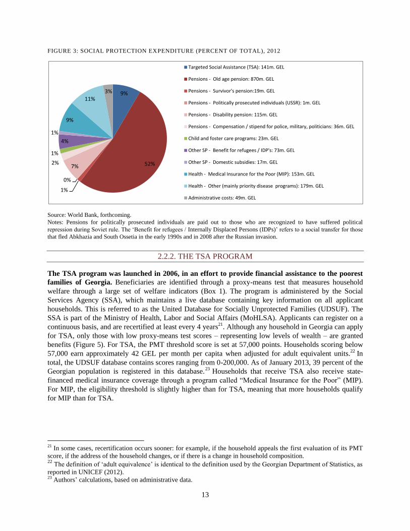
FIGURE 3: SOCIAL PROTECTION EXPENDITURE (PERCENT OF TOTAL), 2012
Source: World Bank, forthcoming.
Notes: Pensions for politically prosecuted individuals are paid out to those who are recognized to have suffered political
repression during Soviet rule. The ‘Benefit for refugees / Internally Displaced Persons (IDPs)’ refers to a social transfer for those
that fled Abkhazia and South Ossetia in the early 1990s and in 2008 after the Russian invasion.
2.2.2. THE TSA PROGRAM
The TSA program was launched in 2006, in an effort to provide financial assistance to the poorest
families of Georgia. Beneficiaries are identified through a proxy-means test that measures household
welfare through a large set of welfare indicators (Box 1). The program is administered by the Social
Services Agency (SSA), which maintains a live database containing key information on all applicant
households. This is referred to as the United Database for Socially Unprotected Families (UDSUF). The
SSA is part of the Ministry of Health, Labor and Social Affairs (MoHLSA). Applicants can register on a
continuous basis, and are recertified at least every 4 years21
. Although any household in Georgia can apply
for TSA, only those with low proxy-means test scores – representing low levels of wealth – are granted
benefits (Figure 5). For TSA, the PMT threshold score is set at 57,000 points. Households scoring below
57,000 earn approximately 42 GEL per month per capita when adjusted for adult equivalent units.22
In
total, the UDSUF database contains scores ranging from 0-200,000. As of January 2013, 39 percent of the
Georgian population is registered in this database.23
Households that receive TSA also receive state-
financed medical insurance coverage through a program called “Medical Insurance for the Poor” (MIP).
For MIP, the eligibility threshold is slightly higher than for TSA, meaning that more households qualify
for MIP than for TSA.
21
In some cases, recertification occurs sooner: for example, if the household appeals the first evaluation of its PMT
score, if the address of the household changes, or if there is a change in household composition. 22
The definition of ‘adult equivalence’ is identical to the definition used by the Georgian Department of Statistics, as
reported in UNICEF (2012). 23
Authors’ calculations, based on administrative data.
9%
52%
1%
0%
7% 2%
1%
4%
1%
9%
11% 3%
Targeted Social Assistance (TSA): 141m. GEL
Pensions - Old age pension: 870m. GEL
Pensions - Survivor's pension:19m. GEL
Pensions - Politically prosecuted individuals (USSR): 1m. GEL
Pensions - Disability pension: 115m. GEL
Pensions - Compensation / stipend for police, military, politicians: 36m. GEL
Child and foster care programs: 23m. GEL
Other SP - Benefit for refugees / IDP's: 73m. GEL
Other SP - Domestic subsidies: 17m. GEL
Health - Medical Insurance for the Poor (MIP): 153m. GEL
Health - Other (mainly priority disease programs): 179m. GEL
Administrative costs: 49m. GEL

14
32.8% of applicants: receiving TSA & MIP
11.6% of applicants: receiving MIP only
55.5% of applicants: rejected applications
0 20,000 40,000 60,000 80,000 100,000 120,000 140,000 160,000 180,000 200,000
Score-group
PMT Score
BOX 1: GEORGIA’S MEANS-TESTING METHODOLOGY
Eligibility for TSA is determined by a proxy means test (PMT) that is administered by the SSA to
any household that applies. The test is based on a complex scoring formula that yields a composite score
based on over 100 household welfare indicators that include economic, demographic, and regional
measures (Figure 4). The overall score also takes into account a subjective assessment of the household’s
welfare, conducted by a government representative.
FIGURE 4: INDICATORS INCLUDED IN COMPOSITE PMT WELFARE SCORE
Source: Ministry of Labor, Health and Social Affairs of Georgia, 2012.
FIGURE 5: SCHEMATIC OVERVIEW OF PMT SCORE-GROUPS
Average Monthly Adult Equivalent per Capita Income level, by score-group:
0 - 57 000 57 001 - 70 000 70 001 - 100 000 100 000 - 200 000
42 GEL / month 97 GEL / month 107 GEL / month 148 GEL / month
Source: Authors’ calculations, based on UDSUF Database, Nov. 2012 and WMS, 2011 (income per capita).
Notes: Income of TSA beneficiary households is adjusted by deducting the amount received from the TSA program.
Composite PMT Welfare Score
Information on Household
Members (gender, age, education,
health)
Ownership of Durables (car, refrigerator, TV, washing
machine)
Possession of agricultural
land and domestic animals
Geographic information
(region, closeness to
district center)
Income (from labor,
pensions, social
assistance, remittances)
Expenditures on durables
(petrol, furniture, residential
repairs)
Living conditions
(no. of rooms in house)
Subjective Assessment by
Interviewer
TSA Eligibility Threshold: 57,000 points

15
The TSA could still expand in terms of coverage, but performs well in terms of targeting accuracy
and generosity. As of 2011, TSA covered 12 percent of the Georgian population (450,000 individuals),
and 38 percent of the poorest quintile (figure 6). While two thirds of the poorest Georgian households are
still not covered by the TSA program, the data on targeting accuracy shows that this is due to the program
size rather than to a lack of accuracy: close to two thirds of benefits accrue to households in the poorest
quintile, which is high in comparison to other countries in the region. At the same time, the TSA is a
relatively generous program: for each household, benefits in 2011 consisted of a core sum of 30 GEL per
month (US$18), complemented by a benefit of 24 GEL per month ($14 USD) per additional family
member. The average family received 78 GEL per month (US$ 47), which made up 26 percent of post-
transfer household consumption (45 percent among the poorest quintile). Average spending per individual
beneficiary was around GEL 29, compared to GEL 20 in 2008. In 2013, after data collection for this
study, benefits were doubled, to a core payment of 60 GEL per month and additional payments of 48 GEL
per family member (Table 1). Figure 7 shows how government spending on the programs has evolved in
recent years.
FIGURE 6: TSA – COVERAGE, TARGETING ACCURACY AND GENEROSITY, 2011
Source: World Bank, ECA SPeeD, based on WMS, 2011.
38
11 6 4 2
35
5
0
10
20
30
40
50
Q1 Q2 Q3 Q4 Q5 Poor Non-Poor
Pe
rce
nt
Coverage (% of households in quintile receiving benefits)
63
19 9 6 4
66
34
0
20
40
60
80
Q1 Q2 Q3 Q4 Q5 Poor Non-Poor
Pe
rce
nt
Targeting Accuracy (% of benefits accruing to quintile)
45
24
16 12
6
43
15
0
10
20
30
40
50
Q1 Q2 Q3 Q4 Q5 Poor Non-Poor
Pe
rce
nt
Generosity (% of post-transfer consumption accounted for by benefits)

16
Notes: 23.3 percent of the Georgian population falls below the poverty line. Average annual consumption among the poor is 502.7
GEL per capita, versus 2129.8 GEL among the non-poor. Income quintiles are constructed on the basis of pre-transfer income.
TABLE 1: RECENT CHANGES IN TSA PROGRAM DESIGN, 2009-2013
2009 2010 2011 2012 2013
TSA Program
Targeting Threshold increased
from 52,000 to
57,000
Certain assets excluded
from scoring formula;
more say for
communities
Generosity Benefit for
additional family
members: increased
from 12 to 24 GEL
Base benefit: increased from 30
to 60 GEL; Benefit for
additional family members:
increased from 24 to 48 GEL
Other
changes
SSA started cross-
referencing databases
Source: World Bank, 2012; World Bank, forthcoming.
FIGURE 7: GOVERNMENT EXPENDITURE ON TSA, 2008-2013
Source: World Bank, forthcoming.
Notes: Expenditure for both programs is displayed in nominal values, and as percentages of total social protection expenditure for
each year.
2.2.3. EVALUATION OF TSA: SATISFACTION WITH PROGRAM IMPLEMENTATION
AND EFFECTIVENESS
Previous studies have identified possible causes for the TSA coverage gap among the poor.
According to a report published by UNICEF and USAID (2011), many of those in the poorest quintile
have heard of the UDSUF database, but still did not apply. Some of these individuals have negative
attitudes to the application system, and some are unaware of the procedures that must be followed.
Particular barriers faced by this group include lacking documention, language barriers, the distance from
the dwelling to the regional office, and a lack of permanent residence status. Three quarters of non-
applicants stated that they did not know how to apply for the database.
91
147 147 140 141
201
9
11 10
10
8
10
0
2
4
6
8
10
12
0
50
100
150
200
250
2008 2009 2010 2011 2012 2013
Pe
rce
nt
Mill
ion
GEL
TSA - nominal TSA - share of total (%)

17
Non-beneficiaries of TSA but who are close to the threshold of eligibility often evaluate the
application process for TSA to be unfair, whereas only very few beneficiaries of TSA say the same
(Figure 8). The most commonly cited reason for perceived unfairness is that the eligibility criteria are
thought to be an inadequate measure for who really needs assistance. The second most cited reason is that
officials do not adhere to the eligibility criteria. It should be noted that these results, though informative,
may be biased due to the subjective standpoint of applicant households who were not granted the TSA
benefit.
FIGURE 8: SHARE OF RESPONDENTS EVALUATING THE APPLICATION PROCESS AS ‘UNFAIR’
Why do you believe the application process was unfair?
Beneficiary
Non-
beneficiary
Eligibility criteria are inadequate 45 56
Application process is too complex for many 18 5
Officials don’t adhere to eligibility criteria 36 38
Officials often accept side payments 2 1
Total 100 100
Source: Authors’ calculations, based on SAHI survey, 2012-2013.
Notes: Only one respondent per household was randomly selected to answer this question.
For beneficiary households, TSA is contributing to household welfare. 82 percent of households report
that their economic situation improved when they started receiving TSA (Figure 12). The two most
commonly cited reasons for improvement are that the TSA helps cover household expenses and that the
TSA provides stable and predictable source of income. At the same time, only 3 percent of recipient
households argue that the TSA provides “enough support” to cover basic expenses.
FIGURE 9: TSA EVALUATION BY RECIPIENT HOUSEHOLDS
6
46
0
10
20
30
40
50
Beneficiary Non-beneficiary
TSA
Pe
rce
nt

18
Source: Authors’ calculations, based on SAHI Survey, 2012-2013.
There does not seem to be a social stigma associated to receiving social assistance in Georgia.
According to data from the Life in Transition Survey (LiTS), people in Georgia mostly believe that
poverty is to be attributed to “injustice in society” or to “being unlucky” (59 percent of respondents),
whereas only a very small share links poverty to “laziness and lack of willpower” (less than 9 percent).
Indeed, data from 2009 suggest that among households receiving TSA, a substantial share of those who
could be expected to work actually did have jobs at the time: among the 55 percent of TSA recipients who
were of working age in 2009, approximately one third was working, and another quarter was looking for a
job. Approximately one sixth was not working because of family or household duties, or because they
were discouraged to enter the labor market. The remainder of working age individuals was inactive for
other reasons, including studies, illness, disability, and being a pensioner.24
Among TSA beneficiaries of
all age groups, those who were inactive because they were either discouraged or did not want to work,
only constituted about 5 percent of the total.
Results from the survey administered for this particular study generally confirm these findings
(Table 2). A vast majority agrees that social benefits are an effective tool to reduce poverty levels in
Georgia. By contrast, only about one third of non-TSA recipients agree that only those in need receive
benefits. Although more than half of all respondents acknowledge that social benefits lead to a more equal
society, over three quarters contend that in the case of Georgia, benefits are too small. Adverse effects of
social benefits, such as making people less willing to look after themselves and their family, and
permitting laziness and a lack of motivation to work, are only acknowledged by few.
TABLE 2: SHARE OF SUBJECTS EXPRESSING AGREEMENT WITH VARIOUS STATEMENTS ON SOCIAL
BENEFITS IN GEORGIA
Beneficiary
Non-
beneficiary
Social benefits are effective tools to reduce poverty levels in Georgia 74 66
Benefits in Georgia are provided only to those people who really need them 62 35
Social benefits are too small to provide effective help for the population 84 81
Social benefits lead to a more equal society 64 50
Social benefits cost businesses too much in taxes or charges 39 35
Social benefits make people less willing to look after themselves and their family 10 20
In Georgia, people receiving pensions / living in a household with pension 10 12
24
UNICEF WMS, 2009 in World Bank, 2012.
12
70
18
0 0
Did the economic situation of your household improve since you started receiving TSA?
Improved a lot
Somewhat improved
Remained the same
Somewhat deteriorated
Deteriorated a lot

19
recipients are not motivated to work
In Georgia, people receiving social assistance are not motivated to work 7 13
In Georgia, people who receive pensions are lazy 7 9
In Georgia, people who receive social assistance are lazy 8 11
Older people get more than their fair share from the government 5 7
Source: Authors’ calculations, based on SAHI survey, 2012-2013.
Notes: Only one respondent per household was randomly selected to answer this question.
3. SAMPLING FRAME, SAMPLING AND DATA
The main analysis uses a regression discontinuity design (RDD) to examine the causal impact of the TSA
program on labor force participation among households that are close to the eligibility threshold. This
section provides detailed information on the sampling method used and the data that was collected.
3.1 SAMPLING FRAME AND SAMPLING
A newly designed survey – henceforth referred to as “the Georgian Social Assistance and Health
Insurance (SAHI) Survey” was administered to a carefully selected random sample of 4006
households, concentrated around two score thresholds: one for TSA and one for the MIP program.
For the current study, a subsample of 2002 households, concentrated around the TSA threshold, was used.
The UDSUF database of the SSA as of August 2012, described in more detail in Section 2.2, was used as
the sampling frame. This database includes basic demographic information as well as the exact PMT score
received by each applicant household. The sample is representative of Georgian households registered in
the UDSUF database around the threshold score at the national, regional and urban/rural levels.
The sampling frame was restricted to only include households with scores deviating from the
threshold by a maximum of 3000 points.25
This means that the sampling frame covers households that,
as of August 2012, fell between 54,000 points and 60,000 points (57,000 points is the eligibility
threshold). If below the threshold, the household qualifies to receive TSA benefits. As of August 2012, 5.6
percent of all applicant households included in the UDSUF database had obtained a score within this
bandwidth.
Among this group, the selection of the final sampling frame was subject to certain conditions to
ensure comparability and data quality, leading to a further reduction in the number of included
households by 21.1 percent. First, those households that had not been re-scored by the SSA since 2010
were excluded, to ensure up-to-date information on households’ overall welfare status. Within the selected
score range, 13.5 percent of households were excluded from the sampling frame for this reason. Second,
25
The overall score range runs from 0 to approximately 200,000. A bandwidth of 3000 points was chosen because,
on the one hand, it included enough households to draw a random sample with enough power to predict relatively
small effects accurately, and on the other hand, it represents a range of scores that is still narrow enough to only
include a relatively homogenous group of households. In order for the treatment and the control groups in the sample
to be proportional to the final sampling frame, the original score range of ± 3,000 points was slightly adjusted. The
adjusted score range includes scores 54,660-60,000. The bandwidth of 3000 was also that used in the earlier study of
TSA in Georgia.

20
households that were included in the database on or after January 1st, 2012 were excluded from the
sampling frame, to ensure that the registration process for all households in the sample had been
completed at the time of data collection and to allow time for program impact. Among the selected score
range, 8.8 percent of households were excluded from the sampling frame for this reason. Third, eligible
households who did not receive benefits as of October 2012 – shortly before fieldwork – were excluded
from the sampling frame, and households who were not eligible but did receive assistance were also
excluded. This was done to ensure that only households with up-to-date administrative records were
included in the sample. Among the selected score ranges, 4.2 percent of households were excluded from
the sampling frame for this reason. Lastly, households were excluded if they were eligible for TSA at the
time of data collection, but had a previous score that was higher than 80,000 points. This was done
because such extreme reductions in scores could reflect erroneous records. Among the selected score
ranges, 4.6 percent of households were excluded from the sampling frame for this reason. In the UDSUF
database as of October 2012, therefore, 4.4 percent of the applicant households fell within the sampled
score range and met these conditions. A distribution of this final sampling frame is shown in Figure 10.
FIGURE 10: SAMPLING FRAME: DENSITIES AROUND THE CUTOFF SCORE
Source: Authors’ calculations, based on UDSUF database, 2013.
Notes: Binsize: 100 points.
As can be seen in Figure 10, there is some “bunching” of households just below the TSA threshold in
the sampling frame. In the early years of the program, scores were smoothly distributed. However, two
recent changes have resulted in bunching below the threshold: first, since 2011, households were given the
opportunity to appeal if their initial score did not fall below the 57,000 threshold. The households filing
for appeal were rescored, and some of them did receive a new score below 57,000. In the final sample, we
introduce extra robustness tests in our models to eliminate any remaining bias as a result of this appeal
process. Second, in 2011, the SSA started to cross-reference its own database with other sources that
contained information on the welfare of specific households. It was found that some households reported
to possess more assets in these other databases. Hence, the PMT scores of these households were likely to
be biased downwards, and they were taken out of the UDSUF database and disqualified from receiving
benefits. This could explain a decrease in the number of households just to the right of the PMT score.
Even without robustness tests, our results would remain valid because households do not have precise
control over their PMT scores. Even if they can attempt to push their score down, they cannot ascertain
that this will result in a score below the threshold. For a regression discontinuity design, the identifying
assumption is that subjects do not have precise control over their scores. This requirement is met, as
explained in Section 4.
0.5
11
.52
2.5
Fre
qu
en
cy (
%)
55000 56000 57000 58000 59000 60000
Score
TSA Sampling Frame

21
The sampling design controls for observable as well as unobservable community-level
characteristics that may impact the results of interest. In particular, and following the sampling design
used in Bauhoff et al. (2010), 6-household clusters were selected within each stratum based on probability
proportional to size. The sample was pre-stratified for urban and rural areas. Clustering adds value to an
RDD design as it allows researchers to control for unobserved characteristics associated with households’
geographic location. In this study, clusters generally include a mixture of applicant- and non-applicant
households, so that observable and unmeasured community-level characteristics that may have an impact
on the investigated outcomes are controlled for. Proportions of beneficiary and non-beneficiary
households and total cluster size vary somewhat due to non-response. We sampled with replacement. The
results presented in this report are adjusted for this specific sampling design.
The final sample is comprised of 2,002 households and 6,575 individuals. This is 10 percent of the
final sampling frame. Table 3 provides a breakdown of the sample by treatment status.26
Annex 1 provides
an overview of the regional composition of the two sample groups, each broken down into their treatment
and control – “beneficiary” and “non-beneficiary” households. Interviews were conducted between mid-
December 2012 and mid-March 2013.
TABLE 3: SAMPLE COMPOSITION
TSA
Number of Households: Beneficiaries 1001
Number of Households: Non-beneficiaries 1001
Total number of individuals 6575
Total number of working age individuals 3904
Source: Authors’ calculations, based on SAHI Survey, 2012-2013.
Notes: Working age individuals cover age groups 15-64 for men and 15-59 for women.
3.2 THE DATA
The response rate was 79 percent, equally distributed among beneficiaries and non-beneficiaries.
Among the 2,002 households, 1,580 were part of the original sampling frame, whereas the remaining 422
households (21 percent) were chosen from a “reserve” sample that was constructed to replace households
in the original sampling frame which could not, or refused to, be interviewed. Reasons for non-response
were similar among beneficiaries and non-beneficiaries. In approximately half of all non-response cases,
nobody was at home or the dwelling was not found.27
Only 1 percent of the original sample (4.75 percent
of non-response cases) refused to participate in the survey.
26
The chosen sample size was based on power calculations designed to identify, at the 5 percent level of
significance, a five percentage point effect on average labor force participation of the TSA program. This effect size
was determined based on the outcomes typically found in similar studies, as well as in previous work in Georgia
itself. The recommended sample size resulting from these power calculations was 1454 households around the TSA
cutoff. The actual sample was about 25% larger than this. 27
Annex 2 presents an overview of reasons for non-response among these 21%. Apart from small variations in
regional composition and household size, there are no systematic differences between the non-response cases and the
rest of the sample. Differences in household size mainly reflect a higher non-response rate among single-individual
households. This is most likely the result of a higher statistical likelihood of missing a one-person household, as
compared to missing any member of a household consisting of several individuals. Indeed, household size is similar

22
Surveyed households were asked to provide information on a range of topics. The survey covers basic
demographic information (such as gender, age, ethnic background and marital status), information on
educational background, information on employment status, type of employment, wages earned, and
employment history, and information on household welfare, consumption and housing conditions. A short,
self-reported evaluation of the TSA program (among beneficiaries) and self-reported behavioral responses
to being granted TSA (among the control group) is also included. A sub-sample was asked to respond to a
number of questions on values and trust.
As expected, the TSA sample is more rural, poorer and less educated than the average Georgian
individual. Table 4 illustrates that even the demographic outlook of the sample differs from that of the
general population: there are less working age individuals in the TSA sample as compared to the
population average. Similarly, the sample is predominantly made up of rural residents, whereas in the
general population, a slight majority is urban. Education levels are also lower in our sample: in particular,
a much larger share of our sample has only completed primary education as compared to the general
population, and fewer individuals have completed tertiary education. Similarly, Table 5 illustrates that on
average, a household in the sample has only 59.5 percent the amount of income of an average Georgian
household, after adjusting for household size and composition, and without taking the TSA benefit into
account.
TABLE 4: BASIC CHARACTERISTICS OF THE SAHI SAMPLE COMPARED TO GEORGIAN POPULATION
TSA Georgian Population
% Women 53.8 52.9 A
% Children (0-15) 18.5 17.3 A
% Working Age B 59.5 65.8
A
% Retirement Age B 22.2 16.9
A
% Rural 62.8 47.3 C
% Compl. Primary Education 22.5 6.9 D
% Compl. Secondary Education 66.8 60.3 D
% Compl. Tertiary Education 10.0 29.5 D
Average Household Size 4.4 4.6 D
Average no. of Children 1.2 1.1 D
Source: Authors’ calculations, based on SAHI Survey, 2012-2013 (TSA.
Notes: A United Nations, Department of Economic and Social Affairs, Population Division (2013). World Population Prospects:
The 2012 Revision, DVD Edition. 2010 data. B The working age is defined as 15-59 for women and 15-64 for men. C World
Bank, World Development Indicators, 2010. D HBS, 2009. Estimates refer to the share of the adult population aged 25+ that has,
as their highest level of education, completed each of the mentioned education levels.
TABLE 5: INCOME & ASSETS IN THE SAHI SAMPLE, BY URBAN / RURAL LOCATION
Urban Rural Total
Average AE per Capita Income, GEL per month
(Total population: 160.8)
154.6**
(5.2)
122.9**
(3.8)
135.4
(3.2)
Median AE per Capita Income, GEL per month 138.7 102.0 117.2
Average AE per Capita Income, without TSA, GEL per month 120.5**
(5.7) 79.6** (4.4)
95.7**
(3.6)
among non-respondent households with scores below the TSA eligibility threshold as compared to those above the
threshold.

23
Median AE per Capita Income, without TSA, GEL per month 113.0 64.3 82.2
% with Internet 0** 11** 5
% with Phone 65 68 66
Asset Indices (range: 0-100): Sample Average
Radio and TV goods 27.50** 24.00** 26.25**
Housing assets 10.75** 18.63** 13.88
Luxury goods 1.57** 2.43** 1.86
Transport goods 0.67 0.33 0.59**
Financial products 28.50 27.25 28.00**
Source: Authors’ calculations, based on SAHI survey, 2012-2013 (TSA sample); and WMS, 2011 (Georgian population).
Notes: Differences in income, consumption and assets between the urban part and the rural part of the sample are not significant
unless marked with a ** (p<0.01) or * (p<0.05). “AE per capita Income” refers to monthly adult-equivalent per capita income.
For details on the composition of the asset indices, see Annex 3.
Not all sampled households in the treatment group have been receiving TSA for the same amount of
time, and some of the households in the control group did receive TSA benefits in the past. In the
models presented in Section 5, we control for the number of years during which the household has
received TSA (Figure 11). Moreover, to the extent that control subjects did receive benefits in the past,
estimates would be lower-bound ones since the control could also exhibit some program effects.
FIGURE 11: HISTORY OF RECEIVING TSA
Source: Authors’ calculations, based on SAHI survey, 2012-2013.
4. EMPIRICAL APPROACH
We use a regression discontinuity design (RDD) to evaluate the impact of TSA on labor force
participation.28
An RDD is uniquely suitable to examine these impacts in Georgia, because it allowa for a
comparison in outcomes between beneficiaries and non-beneficiaries who are highly similar, apart from
the treatment condition. In doing so, a causal interpretation of results requires less stringent assumptions
28
Labor force participation is defined as being either employed or actively looking for work. Employment is defined
as having worked, for at least one hour, during the last 7 days, paid or unpaid. Unemployment is defined as having
tried to find a job or start a business during the past 4 weeks at the time of the interview. Discouragement is defined
as having stopped looking for work, either because the subject believes that there are no jobs available for someone
with his or her qualifications, or because the subject does not know how to search for work.
0
20
40
60
80
100
2006 2007 2008 2009 2010 2011 2012
Pe
rce
nt
of
Ho
use
ho
lds
History of Receiving TSA
TSA Beneficiary TSA Non-beneficiary

24
than other statistical methods. In the case of the TSA program in Georgia, treatment and control groups
can be identified by making use of the PMT scores assigned to applicant households to determine
eligibility for the program. As discussed earlier, the threshold score used to distinguish eligible and
ineligible households is 57,000. The control group consists of households with PMT scores just above
57,000 – i.e. households not receiving TSA.
Following Lee and Lemieux (2010), we estimate:
x=n
Yi = β0 + β1TSAi + β2Scorei + β3Scorei^2 + Σ βiXi + ɛ i (1)
x=1
x=m
Yi = β0 + β1TSAi + β2Scorei + β3Scorei^2 + β4TSAi*ITni + Σ βiXi + ɛ i (2)
x=1
where Y reflects the outcome variable of interest (labor force participation status) for individual i, β0 is a
constant, TSA is a dummy variable indicating whether the individual pertains to a household that receives
TSA benefits (TSA=1 if so; zero otherwise), β1 is the estimated local average treatment effect, β2 and β3
measure the relationship between the score and the outcome29
, and β4 measures the impact of various
interaction terms (ITn). X represents the x’th control variable (ranging from 1 - m)30
, and ɛ i is the error
term. As explained below, certain respondents were not aware of their status regarding the receipt of
benefits or misreported their treatment status. We use administrative records to avoid any bias that may
result from “selective recall” (Bauhoff et al., 2010) or from confusion of the TSA program with other
benefits.
The structure of the data allows us to exploit a sharp jump in treatment at one specific threshold in
the PMT score. This jump is not accompanied by any other systemic differences that might affect
the outcome variable of interest. Although there is some degree of variance in welfare between the
treatment group and the control group, the only sharp jump in income comes from treatment. As
highlighted by Lee and Lemieux (2010), as long as subjects do not have precise control over their
assignment to either the treatment or the control group, an RDD allows for isolation of the treatment
effect.31
The research design meets the key identifying assumptions of an RDD (see Lee and Lemieux, 2010).
First, the assignment variable – in this case, the PMT score – is continuous around the cutoff, and is
determined before treatment. As discussed in Section 2.2, the PMT score ranges from 0-200,000, with no
interruptions within this range. Second, the choice of the cutoff value in the assignment variable is not
driven by anything other than the treatment. There is no reason to believe that factors other than receipt of
29
In addition to a linear and a quadratic relationship, higher-order polynomials were also tested. These were found
not to affect the results. 30
As is discussed below, certain background characteristics, including gender, age, the household’s PMT score and
other socio-economic and educational characteristics were included as controls to account for variation within each
treatment status along these characteristics that matters for the outcome of interest. See Annex 6 for more details. 31
The underlying assumption is that assignment of beneficiary status is properly enforced (Bauhoff et al., 2010). In
reality, there may be cases where expected beneficiaries are in fact not receiving the benefit. However, this seems to
be unlikely. Less than 1% of all sampled households could present a certificate with their score to the interviewer
that indicated a different recipient-status than was recorded in the UDSUF database. Results presented in Section 5
are not sensitive to excluding these households from the sample, nor to using their self-reported treatment status as
opposed to the administrative records.

25
TSA would change abruptly at the cutoff score and thus, affect labor force participation. The formula on
which eligibility for TSA is based has many variables, and, incidentally, labor force participation and
employment are not direct components of the formula.
Third, random assignment to treatment and control groups was tested by examining the statistical
similarity of recipients and non-recipients, based on demographic and socio-economic outcomes (Annex
3). Only very few characteristics are significantly different across the treatment and control group, and
where differences exist, they remain negligible in size. The most important difference between the two
groups is that beneficiaries are more likely to live in rural areas. This is to be expected, as income levels
are generally lower in rural environments, which is picked up by the PMT scoring procedure.
Correspondingly, households in the treatment group have, for example, slightly lower levels of education.
In addition to these differences correlated to urban/rural status, TSA beneficiaries also have slightly fewer
assets (as expected, given the PMT formula). In the models presented below, we control for these
variables where appropriate. We also examine whether the TSA program had differential impacts on the
outcome of interest depending on these variables. We also make separate estimations for rural and urban
samples.
Finally, subjects have only imprecise control over the assignment variable. As discussed in Section 2.2,
the PMT formula used in Georgia is too complex to precisely manipulate, largely due to the fact that the
number of welfare measures on which the score is based is very large. However, as shown in Figure 12,
there is some bunching of households just below the eligibility threshold. As such, one could be concerned
about the possibility of indirect manipulation. For example, households are able to appeal their initial
score, and to be rescored upon appeal, with some possible bias towards getting included in the TSA
program after rescoring.
FIGURE 12: SCORE DISTRIBUTIONS IN THE SAMPLE
Source: Authors’ calculations, based on SAHI Survey, 2012-2013.
Notes: Binsize: 100 points.
Households can get rescored for various reasons. All households in the UDSUF database, get rescored
periodically. A regular re-evaluation of the household’s PMT score is done every 4 years, to examine
whether an adjustment of the PMT score is necessary. In addition, rescoring can also occur for other
reasons, including appeal of the initially assigned score. Households get rescored if there are substantial
changes in living conditions, such as a change of address, a change in household composition, or a change
in employment status. In addition, the SSA recently started allowing households to file for appeal if the
household believed that the assigned PMT score did not accurately reflect actual levels of welfare.
01
23
Fre
qu
en
cy (
%)
55000 56000 57000 58000 59000 60000
Score
TSA Sample

26
The opportunity to appeal one’s score seems to have introduced bunching. As explained in Section
3.1, the PMT score was characterized by a smooth distribution before the appeal process was introduced.
As such, there is a high likelihood that the bunching observed just below the TSA eligibility threshold is
related to the appeal process. However, in the data collected for this study, it is not possible to distinguish
between the various reasons for rescoring, and hence, households that got rescored because of appeal
cannot be isolated. As a proxy, we investigate two groups in particular: households that got rescored
within a very short timeframe, and households that jumped from the non-beneficiary group to the
beneficiary group after rescoring, in particular in cases where rescoring took place within a short period of
time. The first group is of interest because the SSA is obliged to rescore households that file for appeal
within a period of 2 months.
Households that get rescored within a period of 2 months (15 percent of the households included in
the TSA sample) differ from other households on certain observables.32
In particular, beneficiary
households that were rescored within two months have a larger average household size as compared to
other beneficiary households; they more often have young children and youth in the household; they have
more working age household members, and they have fewer pensioners. Non-beneficiary households that
were rescored within 2 months differ from the rest of the non-beneficiary households on the same
observables. In addition, they are more often found in urban environments, and contain more men. In both
the treatment and control groups, there is no difference between those rescored within two months and the
rest of the sample in terms of education levels. Lastly, households rescored within two months that are
currently in the treatment group are characterized by a lower average adult equivalent per capita income
than the remainder of the treatment group. This result is not found in the control group. It remains unclear
whether this is the result of a genuine negative income shock or of a conscious effort to under-report
income in the survey. In the results presented in Section 5, we control for these characteristics. However,
since the two groups could also differ on unobservables that matter for the outcomes examined here33
, we
also control for this group of households as a whole. In addition, we test the sensitivity of our results to
exclusion of these households. This does not affect the results.
In the selected sample, 26 percent of households that were rescored changed from non-beneficiary
to beneficiary status – a share that is almost twice as high as the 14 percent who changed from
beneficiary to non-beneficiary status. If these changes in status simply reflected errors or changes in
family composition or income, one would expect these two numbers to be very similar. The observed
asymmetry could be an indication of manipulation, although it could also reflect the overall worsening of
economic conditions over the observed period (2006-2012) in Georgia, possibly associated with the global
economic crisis.34
Indeed, the share of rescored households that obtained a lower second score – by at
least 1000 points – (58 percent) is much higher than the share of rescored households that obtained a
higher second score by at least 1000 points (38 percent), regardless of what side of the eligibility threshold
the new score was on. Similarly to the first group, those who switch from being non-beneficiaries to
beneficiaries are different on some observables from others in the treatment group.35
In particular, these
32
Descriptive statistics comparing the two groups are available upon request. 33
This would be the case, for example, if members of these households are particularly interested in receiving a
government transfer, and are hence more likely to “game” the system. This would generate bias if these
unobservables are correlated with their interest in working. 34
This would correspond with evidence from the Welfare Measurement Survey, 2011, in which half of all
households surveyed state that their situation had worsened because of the crisis (UNICEF, 2012). 35
Descriptive statistics comparing the two groups are available upon request.

27
“switching” households are likely to be urban.36
In the results presented in Section 5, we control for these
characteristics. To eliminate any potential bias due to unobservables, we test the sensitivity of our results
to controlling for, and to excluding switchers. This does not affect the results.37
Very few households were rescored within 2 months in such a way that they switched from
beneficiary status to non-beneficiary status. Among those who were rescored within 2 months (13
percent of individuals, and 15 percent of households), less than one fifth (2 percent of the total TSA
sample) received a second score that was below the TSA threshold of 57,000 points.
A third issue of concern is a change in the PMT formula in mid-2010. The PMT formula used by the
SSA was changed in mid-2010 in order to let communities play a greater role in reviewing households’
eligibility, and to exclude certain assets which are difficult to measure or to translate into an indicator of
household welfare. However, as shown in Figure 13, we do not observe an increase in the share of
households switching from the control group into the treatment group after mid-2010. As such, it seems
that the change in PMT formula has not contributed to the observed bunching.
FIGURE 13: SWITCHING PATTERNS OVER TIME: SHARE OF HOUSEHOLDS IN TSA SAMPLE
‘SWITCHING’ TREATMENT STATUS, BY THE TIMING OF THEIR LATEST SCORING EVENT
Source: Authors’ calculations, based on SAHI Survey, 2012-2013.
In short, we are confident that the research design meets the identifying assumptions of the RDD
strategy.
36
In the control group, ‘switchers’ – i.e. households that used to be TSA beneficiaries before rescoring – have a
larger average household size, more working age individuals, a lower average age, and, similar to the treatment
group, a different regional composition. 37
At the same time, it should be noted that, when not restricted by the time interval between subsequent scoring
events, a substantial share of the sample switches from control to treatment status. Especially in cases where this
time interval is large, such a switch may have nothing to do with appeal, but may very well reflect a genuine
deterioration of wealth in the Household. As such, we test different specifications, in some of which we add
restrictions based on the time interval between scoring events.
0
10
20
30
40
50
60
70
jan
. 20
10
feb
. 20
10
mar
. 20
10
apr.
20
10
may
20
10
jun
. 20
10
jul.
20
10
aug.
20
10
sep
. 20
10
oct
. 20
10
no
v. 2
01
0
de
c. 2
01
0
jan
. 20
11
feb
. 20
11
mar
. 20
11
apr.
20
11
may
20
11
jun
. 20
11
jul.
20
11
aug.
20
11
sep
. 20
11
oct
. 20
11
no
v. 2
01
1
de
c. 2
01
1
jan
. 20
12
feb
. 20
12
mar
. 20
12
apr.
20
12
may
20
12
jun
. 20
12
jul.
20
12
aug.
20
12
sep
. 20
12
Pe
rce
nt
Change in PMT formula Switched
Average Share of Households 'Switching' Switched from treatment to control
Switched from control to treatment

28
In terms of external validity, there are three main limitations. First, since the sampling frame only
includes households that have applied to the UDSUF database, households that did not apply but that
would have received similar scores are not represented. These households may be systematically different
from those included in the sampling frame. Second, the sampling strategy systematically excludes clusters
that do not have a mix of beneficiaries and non-beneficiaries. Third, results identify average treatment
effects around the TSA eligibility threshold rather than for the total population that receives TSA benefits
(hence we estimate local average treatment effect). These caveats need to be kept in mind when
interpreting the findings of this study.
Next, we discuss the main results.
5. MAIN RESULTS
Statistical analysis suggests that the TSA program generates work disincentives around the
threshold of eligibility, and that these disincentives are concentrated among women. As a first step in
analyzing the impact of TSA on labor force participation, we compare means on labor force participation
rates between beneficiary and non-beneficiary individuals (Figure 14). In households benefiting from
TSA, the female labor force participation rate is 59 percent compared to 62 percent among women in non-
beneficiary households. The difference in means is not significant for men. The number of working age
individuals among TSA beneficiaries – i.e. the treatment group, at 58 percent, is also significantly lower
than the number of working age individuals in the control group (61 percent).
FIGURE 14: LABOR FORCE PARTICIPATION IN THE TSA SAMPLE
Source: Authors’ calculations, based on SAHI Survey, 2012-2013.
Notes: Differences in participation between the treatment and control group are insignificant for the full sample and for men, and
are significant at the 10 percent level for women.
The regression discontinuity analysis confirms this finding. A participation disincentive effect is
found, and once again, this effect is concentrated among women (Figures 15 and 16. Annex 5 provides a
list of means of included covariates, and Annex 6 presents results for the main specifications.38
Similarly,
in models where only men are included, no effect is detected in any of the specifications tested. On the
other hand, in models where only women are included, a conditional effect of 7-11 percentage points is
found in most models. As such, the findings from this survey suggest that able-bodied, non-student
women who live in households that receive TSA are approximately 9 percentage points less likely to join
the labor force, as compared to women living in similar households, but which do not receive TSA.
38
The models shown in Annex 6 are probit models. We also used linear probability models as a robustness check. In
these linear regression models, similar results were found. Results are available from the authors upon request.
64 69
59 65 68
62
0
20
40
60
80
Full Sample Men Women
Pe
rce
nt
Beneficiary Non-beneficiary

29
FIGURE 15: CONDITIONAL EFFECT OF RECEIVING TSA ON LABOR FORCE PARTICIPATION:
SUMMARY OF MODEL SPECIFICATIONS
Source: Authors’ calculations, based on SAHI Survey, 2012-2013.
Notes: See Annex 6 for more details on model specifications. Statistically insignificant effects are portrayed in lighter colors and
without labels.
FIGURE 16: PREDICTED LABOR FORCE PARTICIPATION, BY GENDER
Men: Women:
Source: Authors’ calculations, based on SAHI Survey, 2012-2013.
Notes: Figures reflect the gender-separated equivalents of Model 2 in the basic models reported in Annex 6.
Various falsification tests confirm these findings. As a falsification test, identical regression
discontinuity models were tested for one score below the actual threshold, and one score above the actual
threshold. The score values chosen were 55830 and 58500. No significant differences were found between
subjects below and subjects above these two random scores, supporting the findings presented here.39
Results from labor force participation do reflect a fall in employment and hours worked, rather
than a fall in unemployment. There is a negative impact on employment, and we find a negative impact
on hours worked, conditional on working, among both men and women. Across specifications, TSA
39
In addition, a model was tested where the per capita transfer amount received by the Household was added to the
model as an extra control variable. This did not change the results, and this additional control was not significant.
-6
-9
-11
-7
-11 -9
-14
-12
-10
-8
-6
-4
-2
0
No controls All controls Restricted sample:2/3 of scores
Restricted sample: ½of scores
Restricted sample:No students and
disabledCo
nd
itio
nal
Eff
ect
s (p
erc
en
tage
p
oin
ts)
All Women Men
0.1
.2.3
.4.5
.6.7
.8.9
1
Pro
ba
bili
ty o
f p
art
icip
atin
g
54400 55200 56000 56800 57600 58400 59200 60000
TSA score
0.1
.2.3
.4.5
.6.7
.8.9
1
Pro
ba
bili
ty o
f p
art
icip
atin
g
54400 55200 56000 56800 57600 58400 59200 60000
TSA score

30
receipt reduces men’s work week by 3-5 hours, conditional on working; TSA receipt reduces women’s
work week by 5 hours, conditional on working.40
Among women, results suggest that the participation disincentive effect is particularly large in
younger age groups, and among those who are married and / or have children. Firstly, we find an
interaction effect between receiving TSA and age: the disincentive effect of receiving TSA seems to be
weakened significantly as individuals, and women in particular, get older. This may be related to the
household- and family related responsibilities that many younger women face. In order to examine this in
more detail, we test additional model specifications in which we split the female half of the sample based
on marital status, whether there are children in the household41
, and whether women belong to the age-
group 15-29 or 30-59 (Table 6). Although results must be interpreted with caution due to the restricted
sample sizes, these models suggest that in addition to a concentration of disincentive effects among young
women, being married indeed strengthens rather than weakens disincentives. Similarly, living in a
household with children seems to strengthen disincentive effects.
A simple comparison of means indeed shows that the strongest difference in labor force
participation rates between the treatment- and control group is found when splitting up women of
working age into two age-groups: 15-29 and 30-59 (Figure 27). This result holds when students and
disabled individuals are excluded from the sample. Although there are also differences between treatment-
and control group when women are split by family status, these differences are not found to be statistically
significant. However, once again, these results should be interpreted with caution, due to limitations in
sample size.
TABLE 6: CONDITIONAL EFFECT OF RECEIVING TSA ON LABOR FORCE PARTICIPATION: SUMMARY
OF MODEL SPECIFICATIONS FOR VARIOUS GROUPS OF WOMEN
1 2 3 4 5
Further
sample restrictions:
No Controls All Controls
Restricted
sample:
2/3 of scores
Restricted
sample:
1/2 of scores
Restricted sample: No
students or disabled
All -0.073* -0.108** -0.112 -0.132 -0.090*
Unmarried, no children -0.048 -0.162 -0.179 0.152 -0.104
Unmarried, children 0.018 -0.203 -0.436*** -0.361** -0.145
Married, no children -0.186* -0.135 0.016 -0.010 -0.133
Married, children -0.102* -0.073 -0.099 -0.142 -0.090
Unmarried -0.011 -0.146 -0.280** -0.239 -0.071
Married -0.129** -0.091 -0.093 -0.128 -0.100*
No children -0.125 -0.147 -0.041 -0.082 -0.097
Children -0.044 -0.116* -0.147* -0.156 -0.106*
Women aged <30 -0.115 -0.158* -0.153 -0.224 -0.135
Women aged 30+ -0.069 -0.055 -0.069 -0.070 -0.065
Women <30, controlling
for age & age^2 -0.115 -0.162* -0.185 -0.256* -0.139
40
Results are available from authors upon request. 41
The data used here do not allow for a distinction between a woman’s own children, and children living in the same
household who have a different mother.

31
Women 30+, controlling
for age & age^2 -0.069 -0.053 -0.072 -0.069 -0.064
Source: Authors’ calculations, based on SAHI Survey, 2012-2013.
FIGURE 17: LABOR FORCE PARTICIPATION RATES FOR WORKING AGE WOMEN, BY FAMILY STATUS
Including Students and Disabled:
Excluding Students and Disabled:
Source: Authors’ calculations, based on SAHI Survey, 2012-2013.
Notes: Only the observed differences in participation rates between women in the treatment and control group in two categories
were found to be significant: 1) married women with older children (p=0.09) and 2) single, divorced or widowed women with
both young and older children (p=0.06).
Among women, there are differences in motivation to work between those receiving TSA and those
not receiving TSA. A sub-sample of male and female individuals was asked to respond to questions on
attitudes regarding work and family responsibilities. For example, a larger share of women in the
treatment group as compared to the control group report disagreement when asked whether they would
enjoy having a paid job, even if they do not need the money (Figure 18). Similarly, when women who are
currently out of the labor force are asked whether they would want to work if they could choose without
restrictions, many among the recipient households report that they would not want to work (28 percent of
respondents), whereas this is a much lower share in the control group (19 percent of respondents) (Figure
19).
57 49 64 62 40 68 62 48 70 67 46 71 0
10
20
30
40
50
60
70
80
Unmarried, nochildren
Unmarried,children
Married, nochildren
Married, children Age-group 15-29 Age-group 30-59
Pe
rce
nt
of
Wo
rkin
g A
ge W
om
en
Beneficiary Non-beneficiary Average, beneficiary Average, non-beneficiary
70 64 71 63 48 74 71 66 73 68 58 74 0
20
40
60
80
Unmarried, nochildren
Unmarried,children
Married, nochildren
Married, children Age-group 15-29 Age-group 30-59Pe
rce
nt
of
Wo
rkin
g A
ge
Wo
me
n
Beneficiary Non-beneficiary Average, beneficiary Average, non-beneficiary

32
FIGURE 18: SHARE OF WORKING AGE RESPONDENTS EXPRESSING AGREEMENT WITH THE
STATEMENT: “I WOULD ENJOY HAVING A PAID JOB EVEN IF I DID NOT NEED THE MONEY”
Source: Authors’ calculations, based on SAHI survey, 2012-2013.
Notes: Only one respondent per household was randomly selected to answer this question.
FIGURE 19: LABOR MARKET PREFERENCES: INACTIVE WOMEN AND WOMEN IN THE LABOR FORCE,
WORKING AGE (15-59)
Inactive Women:
55 64
50
78
58 70
49
67
0
20
40
60
80
100
Inactive Participating in the LaborForce
Inactive Participating in the LaborForce
Women Men
Pe
rce
nt
of
Re
spo
nd
en
ts
Beneficiary Non-beneficiary
28 27 22
9 9
1
19
32 34
5 6 2
0
10
20
30
40
…No job at all ...A paid job in thepublic sector
…A job, but the type of job does
not matter
…To start my own business
…A paid job in the private sector
I am fully satisfiedwith my current
situation
Pe
rce
nt
of
Re
spo
nd
en
ts
If I could choose without any restrictions, I would want…
Beneficiary Non-beneficiary
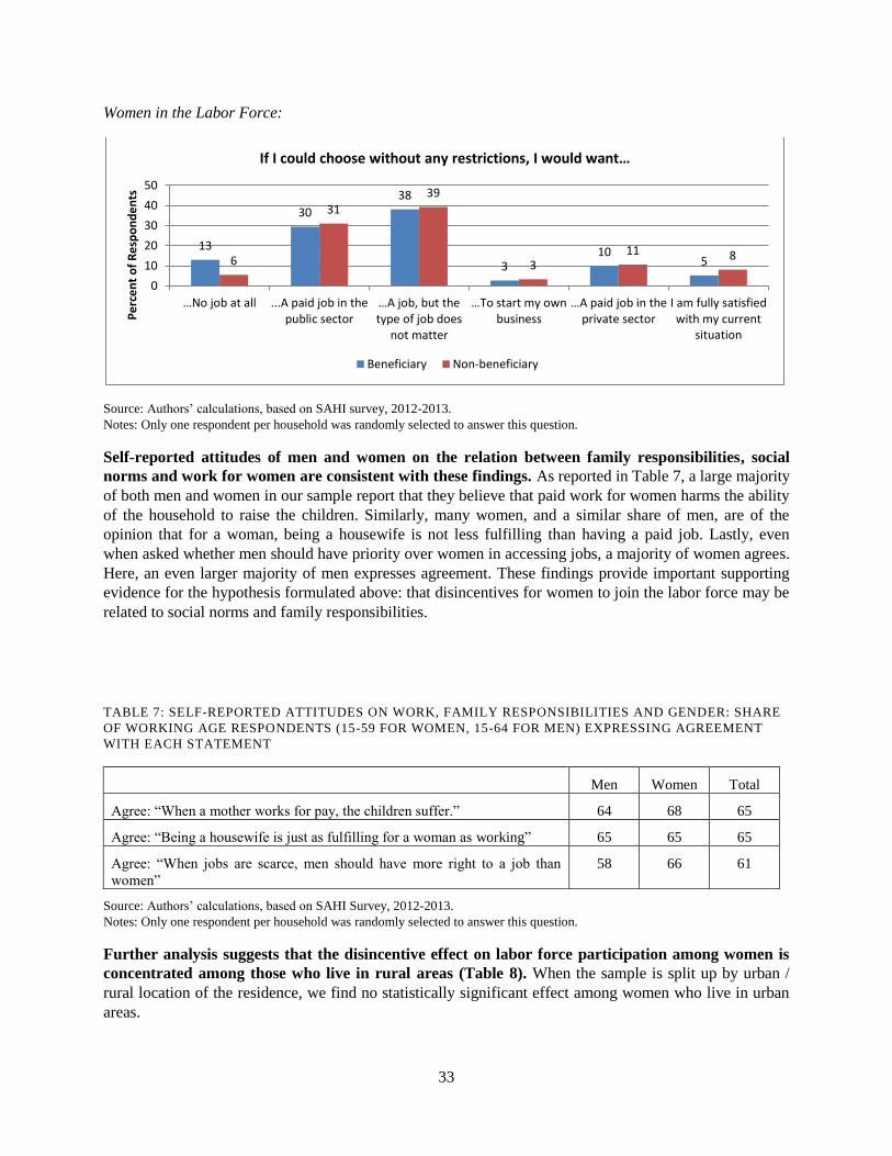
33
Women in the Labor Force:
Source: Authors’ calculations, based on SAHI survey, 2012-2013.
Notes: Only one respondent per household was randomly selected to answer this question.
Self-reported attitudes of men and women on the relation between family responsibilities, social
norms and work for women are consistent with these findings. As reported in Table 7, a large majority
of both men and women in our sample report that they believe that paid work for women harms the ability
of the household to raise the children. Similarly, many women, and a similar share of men, are of the
opinion that for a woman, being a housewife is not less fulfilling than having a paid job. Lastly, even
when asked whether men should have priority over women in accessing jobs, a majority of women agrees.
Here, an even larger majority of men expresses agreement. These findings provide important supporting
evidence for the hypothesis formulated above: that disincentives for women to join the labor force may be
related to social norms and family responsibilities.
TABLE 7: SELF-REPORTED ATTITUDES ON WORK, FAMILY RESPONSIBILITIES AND GENDER: SHARE
OF WORKING AGE RESPONDENTS (15-59 FOR WOMEN, 15-64 FOR MEN) EXPRESSING AGREEMENT
WITH EACH STATEMENT
Men Women Total
Agree: “When a mother works for pay, the children suffer.” 64 68 65
Agree: “Being a housewife is just as fulfilling for a woman as working” 65 65 65
Agree: “When jobs are scarce, men should have more right to a job than
women”
58 66 61
Source: Authors’ calculations, based on SAHI Survey, 2012-2013.
Notes: Only one respondent per household was randomly selected to answer this question.
Further analysis suggests that the disincentive effect on labor force participation among women is
concentrated among those who live in rural areas (Table 8). When the sample is split up by urban /
rural location of the residence, we find no statistically significant effect among women who live in urban
areas.
13
30
38
3 10
5 6
31
39
3 11 8
0
10
20
30
40
50
…No job at all ...A paid job in thepublic sector
…A job, but the type of job does
not matter
…To start my own business
…A paid job in the private sector
I am fully satisfiedwith my current
situation
Pe
rce
nt
of
Re
spo
nd
en
ts
If I could choose without any restrictions, I would want…
Beneficiary Non-beneficiary

34
TABLE 8: CONDITIONAL EFFECT OF RECEIVING TSA ON LABOR FORCE PARTICIPATION: SUMMARY
OF MODEL SPECIFICATIONS FOR URBAN/ RURAL SAMPLE
1 2 3 4 5
Further
sample restrictions:
No
Controls
All
Controls
Restricted
sample:
2/3 of scores
Restricted
sample:
1/2 of scores
Restricted sample:
No students or
disabled
Urban -0.029 -0.052 -0.128 -0.101 -0.039
Rural -0.071* -0.094** -0.115** -0.160** -0.074*
Urban, men 0.002 0.038 -0.030 0.015 0.056
Urban, women -0.058 -0.113 -0.222* -0.208* -0.103
Rural, men -0.065 -0.040 -0.125** -0.174 -0.040
Rural, women -0.086 -0.158** -0.106 -0.143 -0.129**
Source: Authors’ calculations, based on SAHI Survey, 2012-2013.
In addition to age, marital status, family responsibilities and location, low expected productivity
seems to shape labor market decisions. TSA beneficiaries who work earn very low wages. The median
wage of paid workers in the treatment group of our sample is 152 GEL per month, whereas this is 195
GEL per month for the control group.42
In Georgia as a whole, the median monthly wage amounts to 269
GEL.43
In addition, the profile of TSA beneficiaries included in this sample in terms of education level,
geographic location and access to productive assets suggests that the supply of jobs for this group may be
more limited than for individuals that do not qualify for receiving TSA. Yet, despite these differences in
potential earnings, reservation wages among TSA beneficiaries are not statistically different from those of
non-beneficiaries (Figure 20). Critically, reservation wages are significantly higher than the earnings of
beneficiaries actually working. As a result of these forces, inactive TSA recipients may be discouraged to
seek employment because of low anticipated wages, or may decide to stay at home and fulfill house and
childcare responsibilities based on the lower opportunity cost of staying at home. This evidence on
potential earnings and reservation wages suggests that improving the access to training and upskilling of
women in rural areas can be an important part of the agenda for getting them into work outside of their
homes.
FIGURE 20: RESERVATION WAGES AMONG TREATMENT AND CONTROL GROUP
Source: Authors’ calculations, based on SAHI Survey, 2012-2013.
42
Author’s calculations, based on wages reported in the SAHI survey 2012-2013. 43
World Bank (2011).
395 386 380
439
416 416
340360380400420440460
Employed Unemployed Inactive
GEL
pe
r m
on
th
Beneficiary Non-beneficiary

35
Notes: Data represent responses given by one selected individual per household. Among this sub-sample, women and elderly
individuals are overrepresented. The difference between treatment- and control groups was only found to be significant among
employed individuals (P<0.05).
Finally, we find a positive and significant interaction effect between recipient-status and the number
of years during which the household has received TSA in the past. This effect is found in our
aggregate model, which includes both men and women and in our model that includes women only. No
such effect was found in a model including only men. This evidence would be inconsistent with benefit
dependency. On alternative hypothesis is that TSA allows households to build assets over time that could
be used for productive activities, increasing female labor force participation. Given the relevant debates on
benefit dependency, this is one important area for further research.
In short, the results above suggest that work disincentives are concentrated among women who are
young, with children or married, and living in rural areas. Together with the qualitative evidence also
gathered, it appears that the lack of complementary services for raising children, such as affordable
childcare, may be an important constraint to participation. In addition, the evidence on potential and
reservation wages suggests that improving the access to training and upskilling of women in rural areas
can be an important part of the agenda for getting them into work outside of their homes. More research
would be needed to thoroughly investigate what induces disincentives to participate in the labor force.
6. CONCLUSION
The results presented here suggest that recent increases in generosity of Georgia’s TSA program,
such as the increase in benefits for additional family members that occurred in 2009, may have
generated disincentives for women to enter the labor force. The findings from this paper apply
specifically to households around the eligibility threshold of the TSA. However, we have some reason to
think that the TSA more generally could be creating work disincentives. Although not causal evidence,
using a nationally representative survey (UNICEF’s Welfare Monitoring data survey for 2011), we find
that—controlling for basic socio-economic and demographic characteristics— a member of a household
which gets TSA is about 7 percentage points less likely to be working or looking for job compared to
individuals in households that receive no TSA. More research is needed to determine the exact causes of
any disincentive effects among women. However, results here suggest that, for example, disincentives
effects are larger for younger women, and for women who are married and/or have children.
This suggests that in large part, the disincentive effects found from the TSA program in Georgia are
mediated by the lack of appropriate mechanisms for supporting working women, especially when
they are married and/or have children. In such cases, it appears that the TSA program serves as a safety
net that allows these women to care for their children and homes. This is likely to be caused, at least in
part, by a lack of affordable formal childcare facilities, especially in rural areas: for every group of 100
children under the age of 3 in Georgia, there are less than 10 formal childcare spots available, and only 6
in every 100 are actually enrolled44
. What could add to this is low expectations in terms of wages and/or
(types of) jobs available for these groups of women in particular, as outlined in Section 5 above.
Moreover, descriptive evidence from the SAHI survey and preliminary qualitative evidence suggests that
social norms may inhibit women to work as well: many individuals, including women, in Georgia seem to
view the rights and opportunities of men and women very differently when it comes to jobs and labor
force participation. Lastly, our findings suggest that the average TSA recipient is more likely to live in a
rural area and to have a relatively low education level. This may further limit the number of jobs on offer
44
UNECE Statistical Division Database, 2010-2011.

36
for those who receive TSA. For women, if there are no jobs available locally, commuting to work may go
against the norms that are upheld by the community.
The current findings are relevant for Georgia and beyond. In Georgia, these results suggest, firstly, the
need to carefully re-evaluate the design features of the TSA program. One of these is the most recent
generosity-expansion of the program. Given the available evidence on poverty reduction effects, it could
be an option to focus more on coverage of the program and less on (further) expanding generosity. For
example, one option would be to introduce proxy-means testing for (part of) the currently universal
pension benefits, and to divert the thus freed resources to expanding coverage of the TSA program.
Certainly, there are to be trade-offs between expanding coverage and increasing generosity in terms of
overall welfare. However, since new beneficiaries are most likely richer than existing beneficiaries, one
would expect that a given amount of transfers would have smaller disincentive effects than increasing
further the transfer amount for a given group. This is particularly the case given, as is in Georgia, that
disincentive effects seem to arise from an income effect rather than a substitution effect, as suggested by
the lack of impact in the earlier impact evaluation of the TSA before the increase in generosity.
Strengthening the work incentives of social assistance programs is most likely to be successful if
accompanied by measures that assist people in finding work and reduce the costs of working. This
could include incentives to complete higher levels of education or job-specific training, but also for
example incentives for individuals to become more geographically mobile, so that they can move to
locations where jobs are available. Incentives on the side of employers can also help, as can policy
measures that counter normative systems that keep especially women out of work. Policies that facilitate,
or reduce the cost of, high-quality childcare, can go a long way. In addition to formal childcare services,
preschool, for children aged 3-5, and after-school activities for school-aged children could also help
women keep a job while taking care of their children. Yet, as the empirical evidence from these programs
indicate, early education has to be high-quality (Cascio 2015). Results also point to the potential role of
supplemental measures that more directly link benefit receipt with job search, take-up of active labor
market programs and education or training. Where appropriate, this could include an obligation to actively
look for work while receiving the TSA benefit. Balancing policy design with the institutional demands
necessary to successfully implement these policies is necessary. In cases where finding a job is unlikely,
education or training requirements, or participation in active labor market programs, could be used
instead. For women with young children, requirements need to be adapted depending on whether or not
there are childcare options at a sensible distance.
There are several open questions for which additional research would be useful. One area for future
research is to better understand the impact of TSA and other public transfers on private, informal transfers,
to measure the extent to which there is crowding out. If there is in fact crowding out, then public transfers
aimed at helping the poor will be less effective than initially thought and the gains from such programs
would actually be shared with better-off households who are the ones who usually give the transfers. In
other words, if there is crowding out, government transfers will have a limited distributional effect, in
addition to possibly having pervasive effects on the already existing informal risk-sharing arrangements.
In the context of Georgia, a next steps is to aim at measuring the impact of TSA in total household
income. Further research could focus on collecting larger samples of those groups of women that were
found here to be most likely to face disincentives to work as a result of the TSA program. This would
allow for a more granular understanding of the drivers of potential work disincentives. Moreover, the
research agenda could further focus on better understanding how different modalities linking social
assistance with productive employment and search impact labor force participation decisions.

37
REFERENCES
Adato, Michelle and John Hoddinott. (2008). ―Social Protection: Opportunities for Africa.‖ IFPRI
Policy Brief 5. Washington, DC: International Food Policy Research Institute.
Adema, Willem (2006). ―Social Assistance Policy Development and the Provision of a Decent Level of
Income in Selected OECD Countries.‖ OECD Social, Employment and Migration Working Papers 38
Paris: OECD.
Arias, Omar S.; Sánchez-Páramo, Carolina; Dávalos, María E.; Santos, Indhira; Tiongson, Erwin R.;
Gruen, Carola; de Andrade Falcão, Natasha; Saiovici, Gady; Cancho, Cesar A.. 2014. Back to work :
growing with jobs in Europe and Central Asia. Washington, DC: World Bank.
Barr Ben, Stephen Clayton, Margaret Whitehead, Karsten Thielen, Bo Burström, Lotta Nylén, and Espen
Dahl (2010). ―To What Extent Have Relaxed Eligibility Requirements and Increased Generosity of
Disability Benefits Acted as Disincentives for Employment? A Systematic Review of Evidence from
Countries with Well-Developed Welfare Systems.‖ Journal of Epidemiology & Community Health
64(12):1106-14.
Bauhoff, S., D. R. Hotchkiss, and O. Smith. "The impact of medical insurance for the poor in Georgia: a
regression discontinuity approach." Health economics (2010).
Bertrand, M., S. Mullainathan, and D. Miller. 2003. “Public Policy and Extended Families: Evidence from
Pensions in South Africa.” World Bank Economic Review 17(1): 27–50.
Bourguignon, François, Fracisco H.G. Ferreira, and Phillippe G. Leite (2003). ―Conditional Cash
Transfers, Schooling, and Child Labor: Micro-Simulating Brazil‘s Bolsa Escola Program.‖ World Bank
Economic Review 17(2):229–54.
Cascio, Elizabeth. 2015. “The Promises and Pitfalls of Universal Early Education.” IZA World of Labor
116. Bonn.
Eissa, Nada, and Hilary Hoynes (2005). ―Behavioral Responses to Taxes: Lessons from the EITC and
Labor Supply.‖ NBER Working Paper 11729. Cambridge, MA: National Bureau of Economic Research.
Eissa, Nada, Henrik Kleven, and Claus Kreiner (2004). ―Evaluation of Four Tax Reforms in the United
States: Labor Supply and Welfare Effects for Single Mothers.‖ NBER Working Paper 10935. Cambridge,
MA: National Bureau of Economic Research.
Eissa, Nada, and Jeffrey Liebman (1996). ―Labor Supply Response to the Earned Income Tax Credit.‖
Quarterly Journal of Economics 111(2): 605-37.
Freije, Samuel, Rosangela Bando, and Fernanda Arce (2006). ―Conditional Transfers, Labor Supply, and
Poverty: Microsimulating Oportunidades.‖ Economía 7(1): 73-124.
Gasparini, L. F. Haimovich, and S. Olivieri. 2007. “Labor Informality Effects of the Programa Jefes de
Hogar.” CEDLAS Working Paper 53, Centre for Distribution, Labor and Social Studies (CEDLAS),
National University of La Plata, Buenos Aires.

38
Kits, Barbara, and Indhira Santos. forthcoming. “Promoting Labor Market Participation and Social
Inclusion in Europe and Central Asia’s Poorest Countries”. World Bank: Washington, DC.
Lee, David S., and Thomas Lemieux. "Regression Discontinuity Designs in Economics." The Journal of
Economic Literature 48.2 (2010): 281-355.
Lemieux, Thomas, and Kevin Milligan (2008). ―Incentive Effects of Social Assistance: A Regression
Discontinuity Approach.‖ Journal of Econometrics 142(2):807-28.
Mason, A. D. 2007. “Informality, Social Protection, and Antipoverty Policies.” In Informality: Exit and
Exclusion, edited by G. E. Perry, W. F. Maloney, O. S. Arias, P. Fajnzylber, A. D. Mason, and J.
Saavedra-Chanduvi, 179–211. Washington, DC: World Bank.
Medeiros, M., Britto, T., & Soares, F. V. (2008). Targeted cash transfer programmes in Brazil (No. 46).
Working Paper.
Meyer, Bruce D., and Dan T. Rosenbaum (2001). ―Welfare, the Earned Income Tax Credit, and the
Labor Supply of Single Mothers.‖ Quarterly Journal of Economics 116(3): 1063-114.
Rutkowski, Jan (2012). “Skills Mismatch and Unemployment in Georgia: The Challenge of Creating
Productive Jobs,” Washington, DC: The World Bank.
Schneider, H., & Uhlendorff, A. (2005). Transitions from Welfare to Employment: Does the Ratio
Between Labor Income and Social Assistance Matter?. Schmollers Jahrbuch: Journal of Applied Social
Science Studies/Zeitschrift für Wirtschafts-und Sozialwissenschaften, 125(1), 51-61.
Skoufias, Emmanuel, and Vincenzo Di Maro (2008). ―Conditional Cash Transfers, Adult Work
Incentives, and Poverty.‖ Journal of Development Studies 44(7):935-60.
Soares, F. V., Ribas, R. P., & Osório, R. G. (2010). Evaluating the impact of Brazil's Bolsa Familia: Cash
transfer programs in comparative perspective. Latin American Research Review, 45(2), 173-190.
Soares, S. S. D. (2012). Bolsa Família, its design, its impacts and possibilities for the future (No. 89).
Working Paper, International Policy Centre for Inclusive Growth.
UNICEF and USAID, 2011. ‘Survey of Barriers to Access to Social Services: Why not all poor families
get social benefits and services’ http://www.unicef.org/georgia/BASS_final-eng.pdf.
UNICEF, 2012. ‘The Well-Being of Children and their Families in Georgia,’
http://www.unicef.org/georgia/WMSFinal_Copy_for_web.pdf.
World Bank (2011). “Armenia: Social Assistance Programs and Work Disincentives” World Bank Report
No. 63112-AM, Washington, DC.
World Bank, 2012: “Georgia Public Expenditure Review: Managing Expenditure Pressures for
Sustainability and Growth” Auth.: Khan, F., M. Dolidze, O. Smith, A. Schwarz, S. Groom and M.
Pokorny.
World Bank, forthcoming. Georgia Public Expenditure Review. World Bank: Washington, DC.

39
ANNEX 1: REGIONAL SAMPLE COMPOSITION
Source: Authors’ calculations, based on SAHI Survey, 2012-2013.
Notes: Pie-charts reflect proportions of sampled individuals by region. Proportions are not adjusted for the complex sampling
design, but reflect the actual ratios of sampled households.
ANNEX 2: REASONS FOR NON-RESPONSE
Source: Authors’ calculations, based on SAHI Survey, 2012-2013.
Notes: Percentages reflect the reasons for non-response among 21 percent originally sampled but not interviewed.
30
18
14 12
10
6
3 1 1
4
26
21
8 9
11 11
8
1 1 2
0
5
10
15
20
25
30
35
Nobody athome during
visit
Dwelling notfound
No access tothe house
Temporarilyliving
elsewhere
Dwellingabandoned
Anotherfamily lives inthe dwelling
Respondentsrefused toparticipate
Desiredrespondentwas not at
home
Desiredrespondent
was busy or ill
Other
Pe
rce
nt
of
no
n-r
esp
on
se
Beneficiary Non-beneficiary

40
ANNEX 3: DESCRIPTIVE STATISTICS
Household Level Characteristics
Benefi-
ciary
Nonbene-
ficiary
Difference B T-value N
% Urban 36
(1)
43
(1)
7*** 3.12 2002
Household Size 3.24
(0.06)
3.34
(0.06)
.10 1.10 2002
% HH has Pensioners 50
(2)
47
(2)
-3 1.38 2002
% has Internet 2
(1)
7
(1)
5*** 5.21 2002
% has Computer 4
(1)
8
(1)
4*** 4.24 2002
% has Phone 63
(2)
70
(2)
8*** 3.54 2002
Asset Indices (range: 0-100): Sample Average
Radio & TV assets C 25
(1)
27
(1)
2*** 3.16 2002
Housing assets D 12
(1)
15
(1)
3*** 4.45 2002
Luxury assets E 1
(0)
2
(0)
1*** 3.85 2002
Transport assets F 0
(0)
1
(0)
1*** 3.13 2002
Financial products G 32
(1)
24
(1)
-8*** 8.95 2002
Source: Authors’ calculations, based on SAHI Survey, 2012-2013.
Notes: *** p<.01, ** p<.05, * p<.1 A Additional household-level covariates for which the difference in means was analyzed
include: regions, household composition in terms of age groups (no. of youth aged 15-24, no. of prime aged workers aged 25-49,
no. of older workers aged 50-64, and no. of children aged 0-18). For all of these additional indicators, results were either not
significant, or if they were, the difference in means was very small. In particular, in the regions of Mtskheta-Mtianeti and Racha-
Leckhumi, qvemo Svneti, the treatment group represented a significantly larger share of the sample than the control group,
whereas in Tbilisi, the opposite was the case. B A positive number in these columns indicates that the non-recipient group (the
control group) has a higher average than the recipient group (the treatment group). A negative number indicates the reverse. C The
‘Radio and TV Goods’ index includes: Radio set, Satellite Antenna, TV set: flatscreen, TV set: non-flatscreen (Range: 0-4). D The
‘Housing Assets’ index includes: Air Conditioner, Dishwasher, Gas stove / Electric stove, Heater, Oven, Refrigerator, Vacuum
cleaner, Washing machine (Range: 0-8, converted to 0-100). E The ‘Luxury Goods’ index includes: A second dwelling, Camera,
DVD player, Musical Player, Piano or Grand-Piano, Record-player, Video Camera (Range: 0-7, converted to 0-100). F The
‘Transport Goods’ index includes: Bicycle, Car, Microbus or truck, Mini-tractor or motor-block, Motorcycle/quadrocycle, Tractor
(Range: 0-6, converted to 0-100). G The ‘Financial Products’ index includes: Any savings (cash, savings in the bank or other
valuables like gold), a bank account, a debit card, a credit card (Range: 0-4, converted to 0-100).

41
Individual Level Characteristics
Benefi-
ciary
Nonbenefi-
ciary
Difference A T-value N
% Female 54
(1)
54
(1)
0 .15 6575
Age 40.30
(.54)
39.40
(.52)
-.90 1.25 6572
% Youth (15-24) 13
(1)
14
(1)
1 1.41 6575
% Working age E 61
(1)
64
(1)
3** 2.38
6575
% Working age
(Georgian) E
58
(1)
61
(1)
3** 2.27
6575
% Older workers (50-
64)
18
(1)
18
(1)
1 .80 6575
% Married 45
(1)
45
(1)
0 .36 6575
% Ethnic Maj. 93
(1)
92
(1)
0 .34 6575
% IDP Status 3
(1)
7
(1)
4 3.96 6575
% Receives pension 19
(1)
17
(1)
-1 1.24 6575
% can read & write B 99
(0)
100
(0)
1** 2.04
4067
% Educ.: None / Inc.
Prim. B,C
1
(0)
1
(0)
0 1.08 4056
% Educ.: Prim. B,C
23
(1)
18
(1)
-5*** 3.23
4056
% Educ.: Sec. B,C
68
(1)
69
(1)
1 .65 4056
% Educ.: Ter. B,C
8
(1)
12
(1)
4*** 3.54
4056
No. of years formal
educ. B
11.16
(.07)
11.58
(.07)
.42*** 4.75 4017
No. of years work
exp. D
14.90
(.36)
14.83
(.34)
-.08 .17 2619
Source: Authors’ calculations, based on SAHI Survey, 2012-2013.
Notes: *** p<.01, ** p<.05, * p<.1 A A positive number in these columns indicates that the non-recipient group (the control
group) has a higher average than the recipient group (the treatment group). A negative number indicates the reverse. B Sample
restricted to subjects aged 16-65, and not enrolled in grades 1-9. C Education levels were split up as follows: None or Incomplete
Primary, Primary, Secondary (incl. basic/vocational), Tertiary. D Sample restricted to subjects aged 15-64. E ‘Working Age’ refers
to individuals aged 15-64. ‘Working Age (Georgian)’ refers to men aged 15-64 and women aged 15-59. F Additional covariates
for which the difference in means was analyzed include: 5-year age cohorts, and (among those of working age who are without
jobs) the month and year in which the respondent had last worked. For all of these additional indicators, results were either not
significant (which was the case in the MIP sample), or if they were, the difference in means was very small. In particular, the TSA
treatment group had a slightly higher share of individuals aged 70-74, as well as a slightly higher share of individuals aged 80-84
(both had a one percentage point difference). Short-term joblessness (having last worked 1-2 years ago) was slightly less prevalent
in the TSA treatment group as compared to the TSA control group (3 percent vs. 6 percent of jobless subjects in the control
group).

42
ANNEX 4: LABOR FORCE PARTICIPATION BY SCORE GROUP
Aggregate:
Source: Authors’ calculations, based on SAHI Survey, 2012-2013.
Men:
TSA Eligibility Threshold
TSA Eligibility Threshold

43
Women:
Source: Authors’ calculations, based on SAHI Survey, 2012-2013.
TSA Eligibility Threshold

44
ANNEX 5: MEAN VALUES OF COVARIATES – LABOR FORCE
PARTICIPATION
Variable (Range of
values in brackets)
Full Sample Excl. Students &
Disabled
Mean St. Dev. Mean St. Dev.
TSA beneficiary 0.48 0.50 0.48 0.50
Score (54660-60000) 57241 1545 57247 1542
Score squared (2.99E+09-3.60E+09) 3.28E+09 2E+08 3.28E+09 1.77E+08
No. Of years having received TSA (0-7) 2.05 2.16 2.03 2.16
Household was rescored within 2 months A 0.08 0.27 0.07 0.26
Urban 0.38 0.49 0.37 0.48
Household size (1-11) 4.62 1.77 4.63 1.77
Region: Adjara 0.11 0.32 0.11 0.31
Region: Guria 0.04 0.19 0.04 0.20
Region: Imereti 0.20 0.40 0.20 0.40
Region: Kakheti 0.11 0.31 0.11 0.31
Region: Mtskheta-Mtianeti 0.03 0.18 0.04 0.19
Region: Racha-Leckhumi, qvemo Svneti 0.03 0.17 0.03 0.17
Region: Samegrelo, zemo Svaneti 0.11 0.32 0.11 0.32
Region: Samtskhe-Javakheti 0.02 0.15 0.02 0.14
Region: Tbilisi 0.15 0.36 0.15 0.35
Region: Kvemo Kartli 0.07 0.25 0.06 0.24
Region: Shida Kartli 0.13 0.33 0.13 0.33
Household has own business 0.60 0.49 0.61 0.49
Labor intensity in the household B (0-0.857; 0-0.8333) 0.26 0.23 0.26 0.23
Monthly per capita non-wage income,
excl. TSA C (-32.6667-800)
36.53 55.81 34.63 52.67
Interviewer (1-44) 21 13 22 13
Male 0.50 0.50 0.49 0.50
Age 15-19 0.12 0.32 0.06 0.23
Age 20-24 0.12 0.32 0.12 0.32
Age 25-29 0.11 0.32 0.13 0.33
Age 30-34 0.11 0.31 0.12 0.32
Age 35-39 0.10 0.30 0.11 0.31
Age 40-44 0.09 0.29 0.10 0.29
Age 45-49 0.11 0.31 0.12 0.32
Age 50-54 0.10 0.31 0.11 0.31
Age 55-59 0.11 0.31 0.11 0.31
Age 60-64 0.04 0.20 0.04 0.19
Belongs to an ethnic minority 0.06 0.24 0.06 0.23
Education level: None or Incomplete Primary 0.01 0.08 0.00 0.05
Education level: Primary 0.23 0.42 0.20 0.40

45
Education level: Secondary (incl. basic/vocational) 0.67 0.47 0.69 0.46
Education level: Tertiary 0.10 0.30 0.10 0.31
Household has pensioners D 0.36 0.48 0.35 0.48
Family composition: Single/Div./Wid., no children 0.16 0.36 0.15 0.36
Family composition: Single/Div./Wid., young children 0.05 0.22 0.06 0.23
Family composition: Single/Div./Wid., older children 0.16 0.37 0.12 0.32
Family composition: Single/Div./Wid., both young and
older children
0.04 0.19 0.03 0.18
Family composition: Married, no children 0.19 0.40 0.20 0.40
Family composition: Married, young children 0.16 0.36 0.17 0.38
Family composition: Married, older children 0.15 0.36 0.17 0.37
Family composition: Married, both young and older
children
0.09 0.29 0.10 0.30
Subject is the head of the household 0.25 0.43 0.27 0.44
Subject is a student 0.08 0.27
Subject is disabled 0.05 0.23
Obs. 3904 3393
Source: Authors’ calculations, based on SAHI Survey, 2012-2013.
Notes: A Households were only categorized as ‘rescored within 2 months’ if their original score was not below the TSA cut-off
score of 57000. B Labor intensity in the household was defined as the number of working household members, excluding the
subject being analyzed, divided by the total household size. C 2.15 percent of all sampled households reported a TSA income that
was higher than the reported overall household income. Hence, there are a number of overall income values in this variable which
fall below zero. D ‘Pensioners’ are defined as individuals aged 65 and over for men, and aged 60 and over for women, reflecting
the official retirement ages in Georgia.

46
ANNEX 6: LABOR FORCE PARTICIPATION RDD RESULTS
Basic models. Dependent variable: Dummy for Labor Force Participation. Sample: Men and Women,
working age.
(1) (2) (3) (4) (5)
No
controls
All
controls
Restricted
sample: 2/3 of
scores B
Restricted
sample: ½
of scores B
Restricted
sample: No
students and
disabled
TSA Beneficiary -.052
(.034)
-.062*
(.038)
-.092*
(.049)
-.112**
(.057)
-.048
(.034)
Score -.000
(.000)
-.000
(.001)
-.001
(.001)
.001
(.003)
-.000
(.000)
Score squared
.000
(.000)
.000
(.000)
-.000
(.000)
.000
(.000)
Household has been rescored
within 2 months
-.011
(.026)
.015
(.032)
-.001
(.035)
-.003
(.022)
Male
.119***
(.019)
.125***
(.023)
.122***
(.026)
.104***
(.016)
Age
.056***
(.005)
.061***
(.006)
.063***
(.006)
.046***
(.004)
Age squared
-.001***
(.000)
-.001***
(.000)
-.001***
(.000)
-.001***
(.000)
Primary education
.235**
(.107)
.181
(.123)
.215
(.149)
.146
(.122)
Secondary education (incl.
basic/vocational)
.272*
(.144)
.162
(.152)
.218
(.190)
.164
(.182)
Tertiary education
.280***
(.070)
.226**
(.091)
.236**
(.111)
.188**
(.084)
Unmarried, with children
-.004
(.037)
-.031
(.047)
-.051
(.055)
-.010
(.034)
Married, no children
-.069**
(.035)
-.114***
(.040)
-.087*
(.047)
-.066**
(.031)
Married, with children
-.057
(.036)
-.104**
(.045)
-.099*
(.050)
-.055*
(.031)
Head of the household
.110***
(.024)
.121***
(.028)
.120***
(.031)
.097***
(.020)
Student
-.373***
(.047)
-.395***
(.061)
-.357***
(.069)
Disabled
-.674***
(.018)
-.683***
(.023)
-.671***
(.008)
Urban
.089***
(.032)
.046
(.038)
.043
(.040)
.072***
(.028)
Household size
.003
(.008)
.003
(.010)
.005
(.011)
.001
(.007)
Own business
.333***
(.030)
.327***
(.036)
.321***
(.037)
.327***
(.029)
Monthly per capita non-wage
income, minus TSA C
.001***
(.000)
.001***
(.000)
.001***
(.000)
.001***
(.000)
Additional control variables E No Yes Yes Yes Yes
Observations 3,904 3,894 2,533 1,994 3,383
Source: Authors’ calculations, based on SAHI survey, 2012-2013.

47
Basic models. Dependent variable: Dummy for Labor Force Participation. Sample: Women, working age.
(1) (2) (3) (4) (5)
No
controls
All
controls
Restricted
sample: 2/3 of
scores B
Restricted
sample: ½
of scores B
Restricted
sample: No
students and
disabled
TSA Beneficiary -.073*
(.044)
-.108**
(.053)
-.112
(.070)
-.132
(.081)
-.090*
(.050)
Score -.000
(.000)
-.000
(.001)
.002
(.002)
.008**
(.004)
-.000
(.001)
Score squared
.000
(.000)
-.000
(.000)
-.000**
(.000)
.000
(.000)
Household has been rescored
within 2 months
-.020
(.035)
.044
(.042)
.025
(.047)
-.030
(.032)
Age
.061***
(.008)
.062***
(.010)
.060***
(.010)
.053***
(.007)
Age squared
-.001***
(.000)
-.001***
(.000)
-.001***
(.000)
-.001***
(.000)
Primary education
.124
(.142)
.198
(.164)
.191
(.160)
-.049
(.238)
Secondary education (incl.
basic/vocational)
.164
(.156)
.194
(.194)
.208
(.183)
-.029
(.222)
Tertiary education
.231**
(.114)
.261**
(.132)
.247*
(.130)
.076
(.203)
Unmarried, with children
-.008
(.053)
-.051
(.067)
-.067
(.079)
-.011
(.052)
Married, no children
-.120**
(.052)
-.142**
(.064)
-.110
(.074)
-.111**
(.051)
Married, with children
-.101*
(.053)
-.153**
(.065)
-.150**
(.076)
-.096*
(.050)
Head of the household
.089**
(.040)
.097**
(.046)
.093*
(.052)
.092***
(.035)
Student
-.316***
(.068)
-.361***
(.085)
-.381***
(.092)
Disabled
-.629***
(.023)
-.647***
(.030)
-.636
(.)
Urban
.121***
(.044)
.052
(.052)
.061
(.058)
.109***
(.040)
Household size
-.013
(.011)
-.009
(.013)
-.010
(.014)
-.012
(.010)
Own business
.375***
(.040)
.370***
(.047)
.370***
(.050)
.384***
(.039)
Monthly per capita non-wage
income, minus TSA C
.001**
(.000)
.001***
(.000)
.001***
(.000)
.001***
(.000)
Additional control variables E No Yes Yes Yes Yes
Observations 1,970 1,964 1,281 1,024 1,724
Source: Authors’ calculations, based on SAHI survey, 2012-2013.

48
Interaction models. Dependent variable: Dummy for Labor Force Participation. Sample: Men and
women, working age
(1) (2) (3) (4) (5) (6) (7) (8)
Score Score2 Gender
TSA
History Age
Educa-
tion Urban All
P beneficiary terms 0.239 0.363 0.090 0.076 0.014 0.477 0.341 0.134
TSA Beneficiary -1.0***
(.000)
-1.0***
(.004)
-.069**
(.035)
-.077**
(.037)
-.16***
(.055)
-.052
(.349)
-.053
(.037)
-1.000
(.000)
Score -.002
(.002)
-.002
(.002)
-.000
(.000)
-.000
(.000)
-.000
(.000)
-.000
(.000)
-.000
(.000)
-.003
(.002)
Score squared .000
(.000)
.000
(.000)
.000
(.000)
.000
(.000)
.000
(.000)
.000
(.000)
.000
(.000)
.000
(.000)
Household rescored
within 2 months
-0.003
(0.022)
-0.003
(0.022)
-0.003
(0.022)
-0.003
(0.022)
-0.003
(0.022)
-0.002
(0.022)
-0.003
(0.022)
-0.003
(0.021)
Male .104***
(.018)
.104***
(.017)
.083***
(.023)
.105***
(.017)
.104***
(.016)
.104***
(.016)
.104***
(.017)
.085***
(.024)
Age
.046***
(.005)
.046***
(.004)
.046***
(.004)
.046***
(.004)
.045***
(.004)
.046***
(.004)
.046***
(.004)
.044***
(.006)
Age squared -.001***
(.000)
-.001***
(.000)
-.001***
(.000)
-.001***
(.000)
-.001***
(.000)
-.001***
(.000)
-.001***
(.000)
-.001***
(.000)
Primary education .149
(.121)
.149
(.120)
.146
(.121)
.150
(.120)
.149
(.124)
.136
(.235)
.145
(.122)
.158
(.222)
Secondary
education
.169
(.181)
.169
(.181)
.165
(.180)
.171
(.182)
.170
(.187)
.163
(.339)
.163
(.181)
.203
(.346)
Tertiary education .191**
(.083)
.191**
(.081)
.189**
(.082)
.192**
(.081)
.191**
(.084)
.195
(.149)
.188**
(.084)
.211
(.134)
Unmarried, with
children
-.009
(.034)
-.009
(.034)
-.009
(.034)
-.008
(.034)
-.011
(.034)
-.010
(.034)
-.010
(.034)
-.009
(.034)
Married, no
children
-.066**
(.032)
-.066**
(.031)
-.066**
(.031)
-.066**
(.031)
-.064**
(.031)
-.067**
(.031)
-.066**
(.031)
-.064**
(.031)
Married, with
children
-.056*
(.031)
-.056*
(.031)
-.054*
(.031)
-.055*
(.031)
-.054*
(.031)
-.055*
(.031)
-.056*
(.031)
-.052*
(.032)
Head of the
household
.097***
(.021)
.097***
(.020)
.097***
(.020)
.098***
(.020)
.098***
(.020)
.097***
(.020)
.097***
(.020)
.098***
(.022)
Urban .072**
(.028)
.072***
(.028)
.072***
(.028)
.072***
(.028)
.072***
(.028)
.071**
(.028)
.067**
(.033)
.061*
(.033)
Household size .001
(.007)
.001
(.007)
.001
(.007)
.001
(.007)
.001
(.007)
.001
(.007)
.001
(.007)
.001
(.007)
Household has own
business
.329***
(.033)
.329***
(.029)
.327***
(.029)
.329***
(.029)
.327***
(.029)
.327***
(.029)
.327***
(.029)
.333***
(.035)
Monthly income,
minus TSA C
.001***
(.000)
.001***
(.000)
.001***
(.000)
.001***
(.000)
.001***
(.000)
.001***
(.000)
.001***
(.000)
.001***
(.000)
No. of years having
received TSA
-.002
(.005)
-.002
(.005)
-.003
(.005)
-.012
(.008)
-.002
(.005)
-.003
(.005)
-.003
(.005)
-.012
(.008)
Beneficiary * Score .000
(.000)
.003
(.004)
Beneficiary * Score
squared
.000
(.000)
-.000
(.000)
Beneficiary * Male
.044
(.030)
.039
(.030)
Beneficiary * No.
of years received
TSA
.016
(.010)
.016
(.010)
Beneficiary * Age
.003***
(.001)
.003***
(.001)

49
Beneficiary *
Primary education
.023
(.334)
.003
(.348)
Beneficiary *
Secondary educ.
.002
(.348)
-.024
(.356)
Beneficiary *
Tertiary education
-.039
(.378)
-.066
(.396)
Beneficiary *
Urban
.011
(.035)
.023
(.035)
Additional controls Yes Yes Yes Yes Yes Yes Yes Yes
Observations 3,383 3,383 3,383 3,383 3,383 3,383 3,383 3,383
Source: Authors’ calculations, based on SAHI survey, 2012-2013.

50
Interaction models. Dependent variable: Dummy for Labor Force Participation. Sample: Women,
working age.
(1) (2) (4) (5) (6) (7) (8)
Score Score2
TSA
History Age
Educa-
tion Urban All
P beneficiary terms 0.043 0.092 0.036 0.006 0.455 0.191 0.000
TSA Beneficiary -1.0***
(.000)
-1.0***
(.000)
-.137**
(.056)
-.273***
(.084)
-.991
(.744)
-.085
(.056)
1.0
(.000)
Score -.005*
(.003)
-.005*
(.003)
-.000
(.001)
-.000
(.001)
-.000
(.001)
-.000
(.001)
-.004
(.004)
Score squared .000
(.000)
.000*
(.000)
.000
(.000)
.000
(.000)
.000
(.000)
.000
(.000)
.000
(.000)
Household rescored
within 2 months
-.031
(.032)
-.031
(.032)
-.031
(.032)
-.029
(.032)
-.030
(.032)
-.030
(.032)
-.030
(.033)
Age
.053***
(.008)
.053***
(.007)
.052***
(.007)
.050***
(.007)
.052***
(.008)
.053***
(.007)
.050***
(.018)
Age squared -.001***
(.000)
-.001***
(.000)
-.001***
(.000)
-.001***
(.000)
-.001***
(.000)
-.001***
(.000)
-.001***
(.000)
Primary education -.027
(.223)
-.027
(.223)
-.043
(.235)
-.049
(.244)
-.913
(1.495)
-.048
(.239)
-.918
(11.209)
Secondary
education
-.007
(.215)
-.007
(.215)
-.023
(.221)
-.026
(.228)
-.790
(4.666)
-.028
(.222)
-.799
(35.924)
Tertiary education .099
(.186)
.099
(.186)
.082
(.199)
.077
(.208)
-.866
(1.580)
.076
(.204)
-.871
(12.010)
Unmarried, with
children
-.011
(.053)
-.011
(.053)
-.007
(.052)
-.011
(.053)
-.011
(.052)
-.011
(.053)
-.007
(.052)
Married, no
children
-.113**
(.051)
-.113**
(.051)
-.108**
(.051)
-.102**
(.051)
-.111**
(.051)
-.111**
(.051)
-.103*
(.056)
Married, with
children
-.096*
(.050)
-.096*
(.050)
-.092*
(.050)
-.090*
(.050)
-.095*
(.050)
-.095*
(.050)
-.086
(.056)
Head of the
household
.091**
(.036)
.091**
(.035)
.096***
(.035)
.097***
(.035)
.092***
(.035)
.092***
(.035)
.099*
(.053)
Urban .110***
(.040)
.109***
(.040)
.109***
(.040)
.110***
(.040)
.108***
(.040)
.115**
(.045)
.109*
(.058)
Household size -.013
(.010)
-.013
(.010)
-.013
(.010)
-.013
(.010)
-.012
(.010)
-.012
(.010)
-.013
(.011)
Household has own
business
.387***
(.040)
.387***
(.039)
.386***
(.038)
.387***
(.038)
.382***
(.040)
.384***
(.038)
.389***
(.102)
Monthly income,
minus TSA C
.001***
(.000)
.001***
(.000)
.001***
(.000)
.001***
(.000)
.001***
(.000)
.001***
(.000)
.001*
(.001)
No. of years having
received TSA
.004
(.008)
.004
(.008)
-.013
(.011)
.004
(.008)
.003
(.008)
.003
(.008)
-.012
(.011)
Beneficiary * Score .000*
(.000)
-.001
(.005)
Beneficiary * Score
squared
.000*
(.000)
.000
(.000)
Beneficiary * No.
of years received
TSA
.027*
(.015)
.026
(.017)
Beneficiary * Age
.005***
(.002)
.005**
(.002)
Beneficiary *
Primary education
.462
(1.911)
.468
(15.111)
Beneficiary *
Secondary educ.
.892
(3.552)
.905
(25.589)

51
Beneficiary *
Tertiary education
.378
(1.014)
.380
(8.018)
Beneficiary *
Urban
-.012
(.051)
-.001
(.053)
Additional controls Yes Yes Yes Yes Yes Yes Yes
Observations 1,724 1,724 1,724 1,724 1,724 1,724 1,724
Source: Authors’ calculations, based on SAHI survey, 2012-2013.
Notes for basic models:
A Robust standard errors in parentheses. *** p<0.01, ** p<0.05, * p<0.1. B In model 3, 2/3 of the total score range was used
(55440-59000). In model (4), ½ of the total score range was used (55830-58500). C 2.15 percent of all sampled households
reported a TSA income that was higher than the reported overall household income. For these households, income was set to zero. D Reference categories: Education level: None / incomplete primary; Family type: Unmarried, no children. E Additional control
variables include: the number of years during which the household has received TSA benefits in the past, the number of other
individuals in the household that are employed as a share of total household size, regional fixed effects, whether the individual
belongs to an ethnic minority, whether there are pensioners in the household, and interviewer fixed effects.
Notes for interaction models:
A Robust standard errors in parentheses. *** p<0.01, ** p<0.05, * p<0.1. B In all models, students and individuals with a disability
were excluded from the analysis. C Income refers to per capita, non-wage income. 2.15 percent of all sampled households reported
a TSA income that was higher than the reported overall household income. For these households, income was set to zero. D
Reference categories: Education level: None / incomplete primary; Family type: Unmarried, no children. E Additional control
variables include: the number of other individuals in the household that are employed as a share of total household size, regional
fixed effects, whether the individual belongs to an ethnic minority, whether there are pensioners in the household, and interviewer
fixed effects.
Copyright © 2022 FDOKUMEN