1187

“Entrepreneurship and Labor Market Mobility: the Role of Unemployment Insurance”

Alexandre Gaillard and Sumudu Kankanamge

January 2021

Entrepreneurship and Labor Market Mobility: the

Role of Unemployment Insurance*

Alexandre Gaillard† Sumudu Kankanamge‡

This version: January 2021

Abstract

We evaluate the effects of unemployment insurance variations in a general equilibriumoccupational choice model of entrepreneurship. We establish that the occupational flowfrom unemployment to entrepreneurship is remarkably sensitive to unemployment in-surance generosity, corroborating our empirical findings. Beyond direct effects on unem-ployment, we find large reallocations between employment and entrepreneurship relativeto changes in generosity. They contribute to an empirically consistent stable aggregateemployment rate, despite increasing unemployment. We show that an insurance coverage

effect, i.e. a change in the relative riskiness between occupations with respect to generosity,is a key driver of our results.

Keywords: Entrepreneurship, Unemployment Insurance, Labor Market Mobility.

JEL classification: E24, J65, E61.

*We are indebted in no specific order to Arpad Abraham, Mark Bils, Patrick Fève, Christian Hellwig, DirkKrueger, Tim Lee, Benjamin Moll, Franck Portier, and José Víctor Ríos Rull for their useful comments and dis-cussions. We are also very grateful for constructive comments from participants at the 2017 SED in Edinburgh,the XXII Workshop on Dynamic Macroeconomics in Vigo, the 23rd CEF conference in New York, the 22nd T2Mconference in Paris, the 2018 Spring Midwest Macroeconomics Meetings in Madison, the 2018 ESEM in Cologne,the ADEMU conferences in Toulouse (TSE) and Prague (CERGE-EI), and the 2019 Transpyrenean Macro Work-shop. This paper supersedes a previous version titled "Insuring Entrepreneurial Downside Risk". The authors aresolely responsible for any remaining errors or omissions. The authors acknowledge funding from ANR undergrant ANR-17-EURE-0010 (Investissements d’Avenir program).

†Toulouse School of Economics, University of Toulouse Capitole, Toulouse, France. Email: alexandre.gaillard@tse-fr.eu.

‡Toulouse School of Economics, University of Toulouse Capitole, Toulouse, France. Email: sumudu.kankanamge@tse-fr.eu.

1

1 Introduction

The primary function of an unemployment insurance (UI) system is to provide coverage

against the loss of employment. However, both the design of the UI scheme and the accom-

panying regulations are bound to have larger consequences on labor market mobility and

occupations. The literature has extensively discussed the relation between UI generosity and

lower incentives to search for a job. Yet, little is known of the impact of this generosity on the

entrepreneurial sector. In this paper, we study how the design of the UI system, specifically

its generosity, defined as the product between the level of benefits and coverage duration,

conditions the entrepreneurship rate and the flows in and out of this occupation.

Our paper empirically establishes that a higher UI provision significantly reduces the

probability of unemployed individuals selecting into entrepreneurship. The estimate is sig-

nificant and economically large, especially when compared to that of the flow from unem-

ployment to employment. Our empirical study uses the Current Population Survey (CPS)

microdata from 1994 to 2015 and the variation in the regular UI and the extended benefits,

i.e. the Extended Benefits (EB) and the successive Emergency Unemployment Compensation

(EUC) programs, across US states and over time. Similarly to Hsu et al. (2018) in a housing

market context, we identify the effect of a change in UI generosity on the selection into en-

trepreneurship by comparing two groups: the insured unemployed group, eligible following

a layoff and the uninsured group, non-eligible for the UI. In the US, while they represent

only 5 to 6% of the total workforce, unemployed individuals represent 20% of the individu-

als transiting into entrepreneurship. A more generous UI program significantly reduces the

propensity to select into entrepreneurship and to a broader extent, into self-employment. In

terms of magnitude, a standard deviation increase in total regular UI generosity corresponds

to a 10% decline in the likelihood of a transition from unemployment to entrepreneurship

and a 14% decline when considering regular generosity and UI extensions.1

We then introduce a quantitative model and a counterfactual experiment framework to ex-

plain the incentives behind the response to a change in the UI design. Our baseline economy is

an incomplete markets general equilibrium model with endogenous search and occupational

choices designed to capture the main features of the transitional flows between occupations,

specifically occupational flow elasticities and occupational masses relative to UI generosity.1This result is robust to alternative periods and the type of variations used. The magnitude would correspond

to an increase by about 8,000$ in total generosity. It could broadly be illustrated as the difference in total UIgenerosity between the states of Pennsylvania and Michigan.

2

Individuals endogenously select into either employment or entrepreneurship. Employed in-

dividuals are subject to a layoff risk and, upon joining the insured unemployment pool, are

eligible for UI benefits for a specific duration before potentially becoming long-run uninsured

unemployed. Adverse shocks may compel entrepreneurs to cease their businesses and upon

joining the unemployment pool, they are uninsured and not eligible for any UI benefits. An

important aspect of the model is its ability to fully characterize unemployment spells and the

long-run uninsured unemployment status. Our parameterization is able to closely reproduce

the observed occupational flows in the US while the baseline UI system corresponds to that of

an average US state both in terms of duration and benefits level. Our setup also fits a number

of relevant non-targeted moments such as the reproduction of key moments of the income

and wealth distributions.

Our model-based counterfactual experiments framework mimics the ability of a policy-

maker to broadly alter the UI design using two instruments: UI duration and UI benefits. In

a nutshell, it is able to generate an extensive variety of UI generosity situations, well beyond

the empirical variety provided by observing the US states data. It lets us capture key insights

about the effects of varying UI generosity and the sizable repercussions on occupational flows,

occupational masses, and aggregate outcomes while relating them to economic incentives.

Using this framework, we establish that the elasticity to UI generosity of the flow from the

insured unemployed pool to entrepreneurship is negative and almost two times higher than

the corresponding elasticity of the flow to the employment pool. This result substantiates

the idea that higher UI generosity lowers the incentives to exit insured unemployment and

is supported by two well-known effects: a moral hazard and a liquidity effect.2 We uncover an

additional effect related to entrepreneurship that we refer to as the insurance coverage effect: it

is the change in the relative riskiness between two asymmetrically covered occupations with

respect to generosity. In essence, both the values of insured unemployment and employ-

ment respond positively to an increase in UI generosity. Insured unemployed individuals

obtain higher UI benefits, while workers are better insured against the unemployment risk.

However, the value of entrepreneurship is not directly responsive to generosity because en-

trepreneurs are not covered by the UI system. From the perspective of an unemployed agent,

the incentive to search for a job is relative to the gap between the values of employment and2The moral hazard effect captures the change in the marginal incentive to search following a variation in UI ben-

efits that effectively lowers the expected net income gain of taking a job. The liquidity effect captures the variationof the search effort relative to the loosening of the liquidity constraint following a change in UI generosity. Seefor instance Shavell and Weiss (1979), Moffitt (1985), Meyer (1990), Hansen and Imrohoroglu (1992), Hopenhaynand Nicolini (1997), Browning and Crossley (2001) and Chetty (2008) among many others.

3

unemployment while the incentive to start a business is relative to the gap between the values

of entrepreneurship and unemployment. In the end, following an increase in UI generosity,

the incentive to exit unemployment for entrepreneurship reduces relative to the incentive to

exit unemployment for employment. In a broader sense, when UI generosity increases, the

incentive to search for a self-employed activity on-the-job is also lower while the incentive to

search for a job on-the-business is increased. On top of this effect, because an entrepreneurial

activity is contingent on the ability to procure sufficient entrepreneurial capital, the incentive

to exit insured unemployment (or employment) for entrepreneurship, conditional on other

characteristics, appears only beyond a wealth threshold. Augmenting UI generosity increases

that threshold and disincentivize poorer individuals from selecting into entrepreneurship

even further. Overall, the above effects lead to a significant long-run loss in potential total

entrepreneurial sector output.

Our approach also gives an additional perspective to a debated puzzle in the literature

related to UI generosity. On one side, and as discussed above, UI generosity has a significant

impact on labor market flows, especially the depressing effect on the flow out of insured un-

employment. On the other side, as empirically established by Chodorow-Reich et al. (2019)

and Boone et al. (Forthcoming), the effect of UI generosity on the aggregate level of em-

ployment is small or non-significant. Our contribution is to show that the flows into and

out of entrepreneurship play a significant role in shaping the aggregate occupational masses.

In substance, when UI generosity increases, the occupational flow from entrepreneurship to

employment increases while the opposite flow decreases. Because the masses of employed

agents and entrepreneurs are larger than the mass of insured unemployed agents, the reallo-

cation from entrepreneurship to employment is a key factor in counterbalancing the flow out

of insured unemployment. As a result, our model generates an empirically relevant stable

mass of employed individuals in the economy when UI generosity increases. We discuss how

much of the above results rest on the tax menu used to finance the UI system and review

alternative options.

Finally, we investigate the effects of a temporary increase in UI generosity on entrepreneur-

ship by accounting for Extended Benefits during the Great Recession. Consistently with the

existing literature, we find that extensions significantly increase unemployment, but we un-

derline that they generate a persistent and significant decrease in the entrepreneurship rate

and the aggregate entrepreneurial sector output. In terms of magnitude, UI extensions may

be responsible for about a 0.2 percentage points decrease in the entrepreneurship rate.

4

Related Literature Our paper is related to the literature studying the effects of UI on the

selection into entrepreneurship. Røed and Skogstrøm (2014) study the relationship between

the provision of UI benefits on the propensity to start a business and find that the selection

into entrepreneurship increases around the time of insurance exhaustion. In a broader sense,

our paper focuses on the provision of UI benefits and its effect on occupational choices. In

this respect, we are related to the wide literature studying micro-level disincentives to UI

provision from the moral hazard effect, studied in Moffitt (1985) or Meyer (1990) among many

others, to the liquidity effect studied, for instance, in Hansen and Imrohoroglu (1992) and

Chetty (2008). We are especially concerned with the impact of UI variations when one oc-

cupation, e.g. entrepreneurship, is uninsured. None of the above contributions have raised

the question of the importance of UI provision on occupational choices and the underlying

mechanisms. This paper is also related to the quantitative literature on entrepreneurship in

relation to mobility and wealth inequality issues pioneered by Quadrini (2000) and Cagetti

and De Nardi (2006) and to the many policy issues that have been addressed using this frame-

work, e.g. Kitao (2008), Cagetti and De Nardi (2009), or Brüggemann (Forthcoming) among

others. Similarly to our contribution, recent papers address the question of insurance mecha-

nisms in models with entrepreneurship. For instance, Fairlie et al. (2011) focus on the effects

of introducing health insurance and Mankart and Rodano (2015) study the effect of alternative

bankruptcy laws. In addition, our paper is related to the literature providing a quantitative

evaluation of the effects of UI on the labor market, such as Hansen and Imrohoroglu (1992)

or more recently Nakajima (2012). Compared to the latter papers, we carefully model un-

employment spells and insurance exhaustion in a model that features entrepreneurship. On

the empirical front, using CPS data and a similar identification strategy as Hsu et al. (2018),

we show that unemployed individuals respond to UI generosity and are less likely to select

into entrepreneurship. Xu (2019) proposes an empirical evaluation focused on the creation of

unincorporated or incorporated businesses. Our contributions hold for variations in regular

and successive UI extensions as well as a definition of entrepreneurship that controls for busi-

ness ownership. Moreover, we provide a theoretical analysis of the incentive effects at play,

notably, through the insurance coverage effect.

The remaining of the paper is organized as follows. Section 2 presents our empirical con-

tributions. Our baseline model and its parameterization are developed in Section 3. Section

4 discusses the properties of our baseline economy while our main results are reported in

Section 5. Section 6 concludes.

5

2 Unemployment Insurance and Occupational Choice

We first document key facts about the US labor market mobility. We recover quarterly occu-

pational flows using matched monthly CPS data. Individuals are either employed (W), unem-

ployed (U), or self-Employed (SE). In the latter group, we further distinguish entrepreneurs

(E) defined as self-employed business owners which is a common definition of entrepreneur-

ship in the literature (Cagetti and De Nardi (2006), Brüggemann (Forthcoming)).3 We then

empirically establish a relation between UI generosity and the propensity to select into en-

trepreneurship out of unemployment.

2.1 Aggregate occupational flows

We start by characterizing the aggregate flows between occupations from 1997 to 2007. Ta-

ble 1 documents transitions between occupations depending on whether entrepreneurs are

defined as business owners or more generally as self-employed. We see two key takeaways.

Comparing the employment and entrepreneurial activities, the former is significantly more

persistent and flows in and out of it are also significantly less volatile than the latter.4 For

self-employed business owners (resp. all self-employed), we find an average quarterly exit

rate of 6% (resp.7.5%), with 1% (resp. 1.4%) toward unemployment. Moreover, the flows out

of the above activities have differing characteristics: most of the flows out of employment are

toward unemployment whereas most of those out of entrepreneurship are toward employ-

ment. This suggests that many entrepreneurs voluntary quit their businesses for a job while

not experiencing unemployment spells. Second, we find that unemployed individuals are

about 5 times more likely to enter entrepreneurship than workers. When considering self-

employed business owners (resp. all self-employed), 2.4% (resp. 3.7%) of the unemployed

individuals and 0.5% (resp. 0.7%) of the workers start a business each quarter. We see at

least two explanations for this fact: (i) workers are less likely to have the time to search for

business ideas and learn about potential business markets, and (ii) unemployed individuals

may choose to enter entrepreneurship as a better outside opportunity or out-of-necessity. As

a result, while they represent only 5-6% of the workforce, unemployed individuals account

for 20% of the individuals transiting into entrepreneurship.3Appendix A.2 provides further details on the sample selection and variables.4One possible explanation of these flows might be related to the risk faced by entrepreneurs. Herranz et al.

(2015) document that smaller businesses display substantial losses. Moreover, as documented by Astebro andChen (2014), a number of additional papers show that self-employment yields a lower income than employment.

6

Table. 1. Quarterly occupational flows for different definitions of entrepreneurship

Transition (%) Mass (%)Employment Entrepreneurship Unemployment

A. All self-employedEmployment 97.20 (0.36) 0.69 (0.1) 2.11 (0.34) 84.3

Entrepreneurship 6.15 (0.93) 92.45 (1.0) 1.40 (0.40) 10.3Unemployment 46.04 (5.87) 3.72 (1.13) 50.25 (6.0) 5.4

B. Self-employed business ownerEmployment 97.35 (0.36) 0.50 (0.09) 2.15 (0.34) 85.2

Entrepreneurship 4.80 (0.82) 94.22 (0.89) 0.99 (0.34) 9.4Unemployment 47.36 (5.86) 2.40 (0.88) 50.25 (6.0) 5.4

Source: authors’ computations using CPS data from 1997 to 2007. Standard deviations between brackets.

2.2 Heterogeneity in UI generosity

Textbook labor economic theories posit that UI generosity is related to smaller incentives

to exit unemployment and an extensive literature focuses on the efforts to find a job. Yet,

little is known of the effects of UI generosity on occupational choices, especially toward self-

employment and entrepreneurship.

In the following, we exploit the heterogeneity in UI generosity across US states and over

time from 1994 to 2015 to study the impact of the UI scheme on the choice to become en-

trepreneur.5 Over the above period, variations in generosity of regular benefits are quite

large, not only in the cross-section but also over time within states. Each state applies its own

benefit schedule with a typical replacement rate of around 50% of the prior wage of an indi-

vidual. However, the level of benefits is capped at each state’s inflation-adjusted maximum

weekly benefit level, hereafter Max Regularbene f its. At the same time, each state applies a limit

on the number of weeks UI benefits can be claimed, hereafter Max Regularweeks. A maximum

of 26 weeks has been the typical UI duration over the sample period. As such, variations

in regular benefits are mostly driven by changes in the regular weekly benefit amount. Fol-

lowing Agrawal and Matsa (2013) and Hsu et al. (2018), we use the following as a proxy to

generosity of the regular UI benefits in each state as:6

Total Max Regularbene f its = Max Regularbene f its ⇥ Max Regularweeks.

During periods of high unemployment, each state also provides extended benefits to in-5Rothstein (2011) and Farber et al. (2015) study the effect of UI extensions on unemployment exit options. They

focus on the timing of the switch toward employment and the potential disincentive effect. We, however, focuson the effect of UI on the resulting occupational choice.

6Regarding the relation to actual UI benefits, Hsu et al. (2018) show that the elasticity of Max Regularbene f its

to total actual compensation payments at the state level is 1.0. Furthermore, they show that for 60% of thepopulation, benefits are capped, and that Max Regularbene f its captures changes in UI benefits well. To complementthe analysis, we check the robustness of the results against alternative UI generosity measures in Appendix A.3.

7

dividuals exhausting their regular benefits in the form of additional weeks. The Extended

Benefits (EB) and the Emergency Unemployment Compensation (the successive names of this

program having been EUC91, TEUC, and EUC08, we hereafter refer to it as simply EUC) are

such regulations. The above variations of regular benefits become even larger when consider-

ing the state by state activation of these extensions. For instance, during the Great Recession

(GR), heterogeneous emergency extensions (EB and EUC) of UI generosity were activated and

in some states, the duration of UI benefits was extended up to 99 weeks. To represent global

UI generosity including the extensions, we build the following measure:

Total Max Bene f its = Total Max Regularbene f its + Max Regularbene f its ⇥ Max EB EUCweeks,

where Max EB EUCweeks is the number of weeks authorized for the extensions. In other

words, it is the total amount of benefits that an individual falling into unemployment in a

given month could claim over the maximum number of weeks the benefits could be claimed

at that time, including UI extensions when available. Accounting for UI extensions pro-

vides additional variations (in UI duration only) that may generate disincentives toward

finding an active occupation such as self-employment or employment.7 Figure 1 displays

the maximum duration (Max Regularweeks + Max EB EUCweeks), the maximum weekly bene-

fit (Max Regularbene f its), and total claimable benefits (Total Max Bene f its) both for as a US

average and selected US states.

Figure 1. Maximum UI benefits duration and amount: US average and selected states

US stateCA

FL

IL

MA

MI

NY

PA

TX

WA

WI

25

50

75

100

1990 2000 2010

Max

UI d

urat

ion

(wee

ks)

0.4

0.6

0.8

1.0

1990 2000 2010

Max

wee

kly

bene

fit ($

1000

)

0

25

50

75

1990 2000 2010

Tota

l Max

Ben

efits

($10

00)

Left panel: maximum duration (Max Regularweeks + Max EB EUCweeks). Middle panel: maximum weekly benefit(Max Regularbene f its), CPI adjusted. Right panel: total claimable benefits (Total Max Bene f its), CPI adjusted. Theblack line is the average for the US. Grey areas reports the NBER recessions. Further details about our computa-tions can be found in Appendix A.2.Sources: US Department of Labor, significant provisions of state unemployment insurance laws biannual reports.

7Moreover, EB and EUC put even more restrictions on the individuals concerning the active search for a newjob, which are likely to further affect the propensity to select into entrepreneurship.

8

2.3 UI generosity and propensity to start a business

To establish the relation between UI generosity and flows to entrepreneurship, we distin-

guish recently laid off unemployed individuals who are eligible for UI from those who either

voluntarily quit their job or are not eligible for the UI. Our empirical study uses a quar-

terly frequency to obtain sufficient flows toward self-employment. Moreover, we use only

quarterly transitions for which we observe that individuals switched since at least two con-

secutive months to another occupation.8 We distinguish two data panels. Panel A, covering

the 1994-2007 period, excludes the GR and the significant UI benefits extensions that were

then implemented. It will let us study the effects of a change in regular benefits. Panel B,

covering the whole 2008-2015 period, encompasses the impact of all benefits changes includ-

ing UI extensions. It will let us verify whether UI duration adjustments observed during

the GR result in similar findings with respect to regular benefits. Consistently, for a laid off

unemployed individual eligible for UI benefits, we impose that the unemployment duration

does not exceed 30 weeks in Panel A and 99 weeks in Panel B. This corresponds respectively

to the maximum UI duration of regular and extended benefits for Panel A and B.

Based on the definitions of generosity above, Figure 2a shows the flows from unemploy-

ment to self-employment disaggregated by US states for Panel A. The left plot displays a

downward relation between the maximum regular benefits level and flows from the pool of

laid off unemployed individuals to entrepreneurship. Namely, US states that have a higher

maximum regular benefits level tend to have a smaller flow from the laid off unemployment

pool to self-employment. The right plot illustrates that such a downward relation does not

exist for individuals that are unemployed for reasons other than a layoff and not eligible

for UI. The left plot of Figure 2b establishes the same relation for Panel B, i.e. a timeframe

where most of the UI benefits extensions offered after the GR had come into implementation.

Consistently, when taking into account regular benefits as well as EB and EUC extensions,

a higher generosity of UI is related to lower flows from the layoff pool to self-employment.

The right plot shows that for individuals that are unemployed for reasons other than a layoff,

there is again no such relation.

To further establish the relation between UI generosity and flows to entrepreneurship, we8The exact construction of the groups are provided in Appendix A.2. Notice that according to Rothstein (2011),

about half of the displaced workers (eligible for UI) actually receive UI benefits. Although laid off workers are animperfect measure of benefits recipients, only a few out of that group receive them. Therefore, laid off workersappears to be a good proxy for UI eligibility.

9

Figure 2. Average quarterly flow toward self-employment among the unemployed individuals

(a) Panel A: regular UI generosity (Total Max Regularbene f its) for the periods 1994:2007

AK

AL

AR

AZ

CA CO

CTDCDE

FL

GA

HI

IA

ID

ILIN

KSKY

LA

MA

MD

ME

MI

MN

MOMS MT

NC

NDNE

NH NJ

NM

NVNY

OHOK

OR

PARI

SC

SD

TN

TX

UTVA

VT

WAWI

WV

WY

0.00

0.02

0.04

0.06

3.0 3.3 3.6 3.9Log Regular Max Benefits

Flow

Lay

off t

o SE

AK

AL

AR

AZ

CACO CT

DCDE

FL

GA

HIIA

ID

ILIN KSKYLA

MAMD

ME

MI

MN

MOMS

MTNC

NDNE

NHNJNM

NV

NY OH

OK OR

PA RISC

SD TN TXUT

VA

VT

WAWI

WV

WY

0.00

0.02

0.04

0.06

3.0 3.3 3.6 3.9Log Regular Max Benefits

Flow

Non

Lay

off t

o SE

(b) Panel B: regular and extended UI generosity (Total Max Bene f it) for the period 2008:2015

AK

ALAR

AZCA

CO

CTDC

DE

FL

GA

HI

IA

ID

IL

IN

KS KY

LA

MAMD

ME

MIMN

MO

MS

NC

ND

NE

NH

NJ

NM

NV

NY OH

OKOR

PARI

SCSD

TN

TXUTVA

VT

WA

WIWV

WY

0.00

0.02

0.04

0.06

3.5 4.0 4.5 5.0Log Max Benefits

Flow

Lay

off t

o SE

AK

AL

AR

AZ CACO CT

DCDEFL

GAHI

IA

IDILINKY

LAMA

MD ME

MI MNMO

MSMT

NC

ND

NE NH

NJNM

NVNY OH

OK

OR

PA

RISCSD

TN

TXUTVA

VT

WA

WI

WVWY

0.00

0.02

0.04

0.06

3.5 4.0 4.5 5.0Log Max Benefits

Flow

Non

Lay

off t

o SE

investigate whether it holds when we control for characteristics of individuals and US states.

Our key identifying strategy rests on the assumption that state-level changes in regular UI

generosity are independent of factors that might otherwise affect the propensity to select into

entrepreneurship among the unemployed, such as the level of incomes. Hsu et al. (2018) show

that this assumption is supported by the data. The maximum regular UI benefits provided

by a given state are not significantly related to the unemployment rate, average wage, log

real gross domestic product per capita, home price growth, or other unobservable factors

captured by state and year-by-month fixed effects.9 Concerning the use of federal extensions

of UI benefits during the GR, we follow Rothstein (2011) and Hsu et al. (2018) and control

for the endogeneity of the EUC and EB activations by controlling flexibly for smooth cubic

polynomial functions of the state’s unemployment rate. Finally, we identify the effect of UI

generosity on entrepreneurial selection by comparing the impact of state-level changes in UI

benefits between the pool of eligible individuals unemployed after a layoff and the rest of the

unemployed. We estimate the following linear probability model:

Unemp. to Occ.ist

=a + bUI generosityst+ gLayoff

it+ dUI generosity

st⇥ Layoff

it

+ xXit + hZst + ls + µt+ eist

(1)

9We replicate and confirm their findings for our sample and covariates in the Online Appendix 1.2.

10

where Unemp. to Occ.ist

is an indicator of whether individual i in state s and quarter t

is switching to the following specific occupation: Self-Employment in general (SE) or En-

trepreneurship (self-employed business owners) (E). The Unemp. to Occ.ist

variable is di-

vided by the average transition rate from unemployment to the specific occupation over the

sample, such that our estimates will reflect the percentage point change relative to the av-

erage probability of switching. The variable UI generosityst

depends on the specification:

Total Max Regularbene f its for regular benefits or Total Max Bene f its for regular and extended

benefits.10 Xit is a vector of individual characteristics that includes household income brack-

ets, educational attainment, ethnicity, sex, age, age squared, marital status, cubic polynomial

in unemployment duration, and an indicator of whether the spouse is currently employed.

Zst is a vector of time-varying US states characteristics that includes a cubic in the monthly

seasonally adjusted state unemployment rate, annual state log real GDP per capita, log in-

come per capita and a housing price index. Those elements are likely to affect the incentive

to start a business as this decision might be correlated with the economic environment and

serve as controls for the endogeneity of the activation of UI extensions. For panel A, following

Hsu et al. (2018), we use additional controls such as the percentage of unionized employees,

the average wages (in thousand dollars), unemployment insurance (UI) trust fund reserve

(percent of covered annual wages), and an indicator for the fraction of negative UI trust fund

reserve. The latter two variables aim at measuring the fiscal condition of the UI system.

Finally, ls and µt

are states and year fixed effects and eist is an idiosyncratic error term.

The results of our baseline linear probability model are reported in Table 2. Given the

estimates in column (1) and (2) our results indicate that an increase by a 1000$ of Total

Max Regularbene f its is associated with a significant 0.025 (resp. 0.016) percentage points de-

cline in the average probability of switching from unemployment to self-employment (resp.

self-employed business owners) among the laid off workers relative to other unemployed in-

dividuals.11 To put this into perspective, a standard deviation increase in UI benefits, i.e. a

30% increase in average generosity, would lead to an 8.4% (resp. 9.8%) decline in the frac-

tion of insured unemployed individuals moving to self-employment (resp. self-employment10Those variables are centered around their respective means before being interacted with Layoff

itsuch that d

measures the percentage change in the probability of switching to an occupation associated with being laid off(with respect to the mean probability) in a state with an average UI generosity.

11To obtain this number note that an increase by a 1000$ of UI corresponds to an increase of 3.2% of the averageTotal Max Regularbene f its. Therefore, in Panel A, the percentage point number corresponds to -0.78*3.2/100 (resp.-0.50*3.2/100).

11

business ownership). We, however, find no significant relation between regular UI benefits

and the switch toward employment (column 3), which might be due to the quarterly fre-

quency of our sample relative to the regular UI duration (26 weeks). Indeed, we are more

likely to capture effects on the resulting occupational choice rather than disincentive effects

of looking for a job. In Panel B, when accounting for UI extensions (column 4, 5, and 6) with

Total Max Bene f it, we consistently find that an increase in UI benefits reduces the probabil-

ity to switch toward entrepreneurship (column 4 and 5), and employment (column 6). For

instance, given our estimates, a standard deviation increase in Total Max Bene f it (correspond-

ing to a 63% increase) is associated with a significant 7% (resp. 14%) decline in the fraction of

unemployed individuals switching toward self-employment (resp. self-employment business

ownership). Those results are robust to a variety of sensitivity analyses gathered in Appendix

A.3 including alternative UI generosity measures and controls or different sample periods.

Table. 2. Unemployment insurance generosity and probability of exit toward an occupation

Panel A: Regular UI benefits Panel B: Incl. UI extensions

U to SE U to E U to W U to SE U to E U to W(1) (2) (3) (4) (5) (6)

Layoff 2.44⇤⇤⇤ 1.60⇤⇤ 0.24 0.91⇤⇤⇤ 1.19⇤⇤⇤ 0.69⇤⇤⇤(0.65) (0.72) (0.17) (0.31) (0.35) (0.13)

log(Total Max Regularbene f it

) �0.13 �0.37 �0.12⇤

(0.34) (0.45) (0.07)Layoff ⇥ log(Total Max Regular

bene f it) �0.78⇤⇤⇤ �0.50⇤⇤ 0.00

(0.20) (0.21) (0.05)log(Total Max Benefit) �0.26 �0.39 �0.03

(0.15) (0.25) (0.04)Layoff ⇥ log(Total Max Benefit) �0.23⇤⇤⇤ �0.26⇤⇤⇤ �0.10⇤⇤⇤

(0.08) (0.09) (0.03)

Individual & State-year controls Yes Yes Yes Yes Yes YesState and year FE Yes Yes Yes Yes Yes YesObservations 70,471 70,471 70,471 68,703 68,703 68,703

Notes:⇤p<0.1; ⇤⇤p<0.05; ⇤⇤⇤p<0.01. Standard errors, adjusted for clustering at the state level, are reported in

parentheses. This table summarizes the results from linear probability regressions of occupational choice outof unemployment on UI generosity. When uninteracted, the Layoff coefficient measures the effect in a statewith average UI benefit. See text for the list of controls. Estimates are normalized by the mean transition rateof the flow, and can be interpreted as an elasticity relative to that mean transition rate.

The results above show that there is an economically significant and large empirical re-

lation between UI provision and the probability that unemployed individuals select into en-

trepreneurship. However, this relation is measured under partial equilibrium conditions and

leave the question of economic performances unanswered.

12

3 Model

We build an incomplete markets dynamic general equilibrium model of entrepreneurship

with occupational flows and search frictions. A unit measure of ex post heterogeneous agents

can be either employed, entrepreneurs or unemployed. Entrepreneurs hold small businesses

and together with a representative corporate firms sector provide the production of the econ-

omy. The model characterizes the path of maximum UI benefits and duration and lets us

study the interaction between UI generosity and entrepreneurship.

3.1 Corporate sector

A representative corporate firm produces Yt using a Cobb-Douglas technology, with total

factor productivity A, capital level Kt and labor Lt, such that: Yt = F(Kt, Lt) = AKat

L1�at

,

where a 2 (0, 1) is the capital share. Profit maximization produces the competitive prices:

rt = Aa⇣

Lt

Kt

⌘1�a� d and wt = A(1 � a)

⇣Kt

Lt

⌘a, with wt and rt the wage and interest rates, and

d the depreciation rate in both the corporate and entrepreneurial sectors.

3.2 Households

The economy is populated by a continuum of infinitely-lived households distributed uni-

formly over [0, 1]. Every period, each agent falls in one of three occupations ot 2 O ⌘

{e, w, u}: entrepreneurship (e), employment (w), or unemployment (u). We keep using the

{E, W, U} notations to designate respectively entrepreneurs, workers and unemployed indi-

viduals. Life-time utility is derived from consumption ct and disutility from search:

Ut = E0

"•

Ât=0

btu(ct, se,t, sw,t)

#, (2)

where se,t is the search effort exerted to start a business and sw,t is the job search effort. b is

the discount factor. Labor is supplied inelastically and the utility function is of the form:

u(c, se, sw) =c

1�s � 11 � s

� syw

w � sye

e , (3)

with ye and yw the search elasticities.

We denote at 2 A the savings of an agent with rt the corresponding deposit interest rate.

In the following, we drop the time index t.

13

Exogenous processes All individuals are endowed with a persistent component q 2 Q that

we call ability. The labor income of a working household, the replacement income of an

unemployed individual, and the business income of an entrepreneurial household all depend

on this ability.12 This component follows the process: log(q) = rq log(q�1) + eq , with eq ⇠

N (0, sq) and Pq the invariant distribution.

Workers are subject to an additional persistent idiosyncratic shock y 2 Y on their labor

income that we call match-quality.13 It follows the process: log(y) = ry log(y�1) + ey, with

ey ⇠ N (0, sy). For a new worker, this shock is drawn from the invariant distribution Py.

Finally, entrepreneurs face a persistent idiosyncratic business shock z 2 Z following:

log(z) = rzlog(z�1) + ez, with ez ⇠ N (0, sz). A new entrepreneur draws her initial shock in

the invariant distribution Q(z).

All idiosyncratic shocks above are realized at the beginning of the period before agents

take any decision. All processes are discretized into a Markov process.

Unemployment Insurance The exact number of remaining periods with UI benefits is an

important component of our model. This component is tracked by the state variable j 2

{0, ..., J} ⌘ J , the remaining number of model periods with UI benefits. We note {b(q, j)}j=0j=J

the path of UI benefits. J is the exogenous regulatory maximum UI duration converted to

model periods but, due to discretization, this number can fall between two model periods.

To implement the exact number of regulatory UI benefits periods, we set J as the number of

model periods immediately above J and then apply a linear rule to provide only partial UI

benefits in the last model period before losing coverage. UI benefits in the current period are:

b(q, j) =

8>>><

>>>:

µwh(q)(1 � t) , j 2 [2, J],

µwh(q)(1 � t)h1 � (J � J)

i, j = 1,

0 , j = 0,

(4)

where w and t denotes aggregate wage and income tax levels. µ is the replacement

rate. With the above rule, agents can be either insured (j > 0) or uninsured (j = 0). In

our benchmark setup, following UI eligibility rules, only a worker falling into involuntary12In addition, we allow individual productivity to evolve in order to generate additional saving motives. Our

model does not take into account life-cycle aspects, human capital accumulation at work, technological progress,or health risks. Those elements can also explain a large productivity dispersion along the life-cycle.

13This model does not include an explicit matching process but y can be viewed as a match-quality componentbecause it starts and ends with a specific job while not appearing as a state for the unemployed or the entrepreneur.This process brings our generated distributions and transitional flows closer to the data.

14

unemployment (i.e. after a layoff) can claim any benefits.

Value functions and states With j the unemployment insurance status, the value function of

a worker is W(xw, j) with state vector (xw, j) 2 w ⇥J and xw ⌘ (a, q, y) 2 w ⌘ A⇥ Q ⇥Y .

An entrepreneur has the value function E(xe, j) with state vector (xe, j) 2 e ⇥ J and xe ⌘

(a, q, z) 2 e ⌘ A⇥ Q ⇥ Z . An unemployed individual has the value function U(xu, j) with

state vector (xu, j) 2 u ⇥J and xu ⌘ (a, q) 2 u ⌘ A⇥ Q. Consistently with the current US

unemployment insurance scheme, workers are assumed to have maximum insurance duration

(i.e. j = J) while entrepreneurs are uninsured (i.e. j = 0).

3.2.1 Workers

Workers earn labor income h(q)yw, where the function h : q 7! maps their individual

ability q into a working ability. They have a probability h = h(q) of getting laid off. In such a

case, they face insured unemployment and can expect to get continuation value U(x0u, J).14 By

providing effort se, workers can search for business ideas on-the-job and start a business in the

next period with probability pe(se).15 They then voluntary change their occupation, lose their

rights to UI claims and can expect a continuation value E(x0e, 0). Their recursive program is:

W(xw, J) = maxc,a0,se

u(c, 0, se) + bEn(1 � h)

hW(x0w, J) + pe(se)max

�E(x0e, 0)� W(x0w, J), 0

i

+ hhU(x0u, J) + pe(se)max

�E(x0e, 0)� U(x0u, J), 0

i ��� y, qo

,

(5)

s.t. c + a0 (1 � tw)h(q)wy + (1 + r)a,

c > 0, a0� 0, se � 0,

(6)

(7)

where tw is a proportional labor income tax and equation (6) the worker’s budget constraint.

3.2.2 Unemployed individual

Insured unemployed individuals (j > 0) receive benefits b(q, j), in proportion to their indi-

vidual productivity q. By claiming UI in the current period, they shift from j periods of

remaining UI rights to j � 1 at the end of the period. Non eligible individuals and those who

have exhausted their rights (j = 0) receive no benefits. Moreover, all unemployed individuals

are assumed to receive a fixed amount m from domestic production. Unemployed individ-

uals search for both a business idea and a job opportunity with respective efforts se and sw

14Notice that in the model, U(xu, j) < W(xw), 8(xu, xw, j). Therefore, we rule out any voluntary transition tounemployment. Conversely, unemployed individuals getting a job opportunity always return to employment.

15Business search effort can describe market research on the feasibility of an idea, competition assessment,business education, agency costs or the time needed to fill administrative forms, validate product norms, etc.

15

and corresponding success probabilities pe(se) and pw(sw). Upon finding a job, they become

workers with continuation value W(x0w, J). Similarly, upon having an idea, a business can be

started in the next period with continuation value E(x0e, 0). Their recursive program is:

U(xu, j) = maxc,a0,se,sw

u(c, sw, se) + bEn

pw(sw)hW(x0w, J) + pe(se)max{E(x0e, 0)� W(x0w, J), 0}

i

+ (1 � pw(sw))hU(x0u, j

0) + pe(se)max{E(x0e, 0)� U(x0u, j0), 0}

i ��� qo

,

(8)

s.t. c + a0 m + b(q, j) + (1 + r)a,

c > 0, a0� 0, se � 0, sw � 0, Equation (4),

(9)

(10)

where equation (9) is the corresponding budget constraint.

3.2.3 Entrepreneurs

Entrepreneurs invest capital k in their self-employed business and operate the technology:

f (k, q, z) = zg(q)(k)n, (11)

with n 2 (0, 1). The function g : q 7! maps individual ability into entrepreneurial ability.

To invest k, entrepreneurs can borrow from a financial intermediary funds that can only be

invested in the business. Recalling that a is the current wealth of an agent, entrepreneurs

choose whether to borrow (k > a) or save (k < a). If they borrow the amount (k � a),

we assume that it is only up to a fixed fraction l of their total assets.16 Entrepreneurial

profit pr is defined as entrepreneurial production net of capital depreciation, any interest

repayment, and the fixed cost c f . The latter accounts for all the additional functioning costs

that entrepreneurs have to bear. By providing effort sw, entrepreneurs can search for a job

opportunity on-the-business and change occupation in the next period with probability pw(sw)

and value W(x0w, J). Otherwise, if they choose to quit entrepreneurship, they can return to

the uninsured unemployment pool with value U(x0u, 0). Their recursive program is:

E(xe, 0) = maxc,a0,k,sw

u(c, sw, 0) + bEy0,q0,z0n

pw(sw)max{W(x0w, J), E(x0e, 0)}

+�1 � pw(sw)

�max{U(x0u, 0), E(x0e, 0)}

��� z, qo

,

(12)

16This type of borrowing constraint have been widely used in the context of entrepreneurship, see for exampleKitao (2008), Buera and Shin (2013) and Brüggemann (Forthcoming) among many others.

16

s.t. c + a0 = (1 � tp)pr(k, q, z) + a + r(a � k) {ka},

pr(k, q, z) = f (k, q, z)� dk � r(k � a) {k�a} � c f ,

k la,

c > 0, a0� 0, sw � 0.

(13)

(14)

(15)

(16)

Equation (13) is the budget constraint and equation (15) is the borrowing constraint.17 tp

is a payroll tax rate paid by entrepreneurs.

3.3 Government

The government runs an UI system that covers the pool of recently laid-off unemployed

individuals and finances it using labor income and payroll taxes. In our benchmark economy,

we assume that UI is equally financed using by a symmetric tax scheme on entrepreneurs

and workers, such that t = tw = tp.18 Total government revenues (T) are:

T =Z

j

Z

xw

twh(q)wy dG(xw, j) +Z

xu

twb(q, j) dG(xu, j) +Z

xe

tppr(k, q, z) dG(xe, j), (17)

with G(xo, j) the mesure of individuals in occupation o with remaining UI duration j. Total

government expenditures G are equal to the allocated UI benefits:

G =Z

j

Z

xu

b(q, j) dG(xu, j). (18)

3.4 Equilibrium

A stationary recursive equilibrium in this economy consists of a set of value functions W(xw, j),

U(xu, j), E(xe, j), policy rules over asset holdings a0(xo, j), consumption c(xo, j), job search ef-

fort sw(xo, j), business search effort se(xo, j), business investment k(xe, j), occupational choices,

prices (r, w) 2 R+, tax rate t 2 R+ and a stationary measure over individuals G(xo, j) 8o, j,

such that: (i) Given prices (r, w) and tax rate t, the policy rules and value functions solve

household individual programs; (ii) The wage w and the interest rate r are equal to the

marginal products of the respective production factor in the corporate sector; (iii) goods and

factor markets clear: (a) capital:R

a0(xo, j)dG(xo, j) = K + K

E, with aggregate entrepreneurial17Recall that the cash on hand of entrepreneurs in the baseline case can be written: f (k, q, z) + (1 � d)k � (1 +

r))(k � a) {k�a} + (1 + r)(a � k) {ka}. Rearranging terms yield profit and budget constraint equations.18In the US, entrepreneurs pay a self-employment tax and workers a labor income tax. However, Anderson

and Meyer (2000) argue that average industry tax rates are largely passed on to workers through lower earnings.We choose a common benchmark tax rate between occupations in order to not significantly distort occupationalchoices in counterfactuals experiments. We discuss the consequences of this assumption in section 5.

17

capital KE =

Rk(xe, j)dG(xe, j), (b) the measure of corporate workers

RdG(xw, j) is equal to

corporate labor demand; (iv) G(xo, j) is the stationary measure of individuals induced by the

decision rules and the exogenous Markov processes; (v) t balances the government budget

(T = G). Finally, we define total output Y as the sum of corporate sector output Y and

entrepreneurial sector output YE

Y = Y + YE = Y +

Z

xe

f (k(xe), q, z)dG(xe, j). (19)

This model has no analytical solution and must be solved numerically. We detail our

numerical implementation for this problem in the Online Appendix 3.19

3.5 Discussion and assumptions

We now briefly discuss a number of modeling assumptions we made.

Employment and job finding/separation A number of papers (for instance Cagetti and

De Nardi (2009) and Brüggemann (Forthcoming)) introduce entrepreneurial labor demand.

While such a framework appears more realistic, it is still very closely related to our current

setup. In static versions of models with entrepreneurial employment, workers are hired in

proportion to their entrepreneurial capital k, productivity q and business shock z.20 Mechan-

ically, in such a case, a higher number of entrepreneurs lead to higher labor demand. This

translates into a higher wage rate which comes at a cost for entrepreneurs but benefits the

workers, and in turn, reduces the entrepreneurship rate. In our setup, instead, more en-

trepreneurs lead to fewer workers in the corporate sector (keeping the unemployment rate

constant), which leads to a higher wage rate w. Employment becomes more attractive and

the number of entrepreneurs reduces. In the end, it is not obvious that our setup needs to be

extended in the entrepreneurial labor direction to better fit the dynamics of the data.

Making the job finding/separation rates endogenous would generate an additional gen-

eral equilibrium mechanism. Clearly, the inclusion of vacancy posting in the entrepreneurial

and corporate sectors may propagate even further the impact of a change in the UI system by

raising hiring costs for entrepreneurs and hence reducing their labor demand. At the same19Specifically, we solve the model using the Endogenous Grid Method (EGM) allowing for type 1 extreme value

shock as in Iskhakov et al. (2017) to smooth the kinks arising from the discrete occupational choice.20It can be shown that if f (k, q, z, n) = zg(q)kn

nx and entrepreneurs pay the a wage bill wn as in most of

the literature with labor demand, the optimal condition is given by n(k, q, z) =⇣

xzg(q)kn

w

⌘ 11�x and f (k, q, z, n) =

(1 � x)zg(q)knn(q, z, k)x .

18

time, a lower labor demand would lead to lower wages, which in turn, would increase labor

demand. We believe this channel to be especially relevant in the short-run. As the main con-

cern of this paper is how occupational risks and choices are important for assessing the effects

of unemployment benefits and, for the sake of parsimony, we leave this for future research.

Bankruptcy As in Mankart and Rodano (2015), a version of this model considers bankruptcy

on unsecured entrepreneurial debt and as a result features more complex dynamics between

occupations.21 However, results are mostly identical. Indeed, bankrupt entrepreneurs consti-

tute a very small fraction of the observed flows out of entrepreneurship. Moreover, we did

not find significant interactions between the UI policy and entrepreneurial bankruptcy.

Learning In the Online Appendix 2.3 of this paper, we provide an additional robustness

test regarding the introduction of business maturity and a form of learning upon the start of

businesses. This specification does not change the qualitative message of the paper.

3.6 Parameterization

We parameterize the model to match key features of US occupational mobility, entrepreneur-

ship as well as cross-sectional moments. Our data counterparts are taken from the CPS and

the Survey of Consumer Finances (SCF). A model period is two months.22

3.6.1 Exogenous parameters

The share of corporate capital a is set to 0.33. We normalize the TFP parameter A to unity.

The depreciation rate d is set to 0.013. The coefficient of relative risk aversion s is set to 1.5.

To closely match CPS transition flows, each period, a fraction z = 0.65% of individuals retires

and is replaced by z uninsured unemployed individuals that enter the workforce.

The persistent individual working ability h(q), the transitory match-quality y, and the

business shock z all follow an AR(1) process in logs. We normalize h(q) = q. The persistence

rq is set to 0.985, corresponding to 10 years in the model, and the variance s2q to 0.21 in

order to generate an earnings Gini coefficient of 0.36. For the match-quality, ry is set to 0.85,

corresponding to a persistence of about a year. The variance of the innovation s2y is set to

0.0225. For the idiosyncratic business process z, we set sz to 0.24 and the persistence is fixed21This alternative version is available upon request.22We produce robustness checks for a lower and a higher frequency of the model periodicity. Results are

qualitatively similar. This periodicity was chosen because transition flows in and out of entrepreneurship in thedata have more observations as compared to a monthly (or lower) frequency.

19

to 0.91, which is equivalent to 0.55 annually and is consistent with the estimates used in

Clementi and Palazzo (2016).23

The search elasticities yw and ye are both set to 2.0 to generate quadratic search costs. We

use a linear relation to characterize the W ! U transition with respect to earnings in the CPS.

We therefore specify the layoff probability h(q) as a function of h(q), such that:

h(q) = ah + bhwh(q), (20)

where ah and bh are estimated using earning quantiles as a proxy for wh(q). We obtain

h(q) = {0.024, 0.017, 0.010}. The benchmark UI replacement rate µ is set to 0.45, close to the

average US state replacement rate in the last decades, and the UI duration is set to J = 3,

which corresponds to 26 weeks. As Kitao (2008), we set the maximum leverage ratio l to 1.5.

3.6.2 Endogenously calibrated parameters and targeted moments

Job and business finding rates The probabilities of getting a business idea or a job oppor-

tunity, pe(se) and pw(sw), arrive at a Poisson rate:

pe(se) = 1 � e�kese , pw(sw) = 1 � e

�kwsw ,

with ke and kw the matching parameters. kw is set to capture the 38.5% of unemployment

individuals transiting toward employment as observed in the CPS, and ke is set to match the

fraction of entrepreneurs. The literature considers various measures of entrepreneurship. For

example, Quadrini (2000) considers self-employment as a first definition and a household

with a participation in a business as another definition. He argues that the results are close

using the two concepts and find a fraction of entrepreneurs of 12%. Based on this, Kitao

(2008) target a fraction of entrepreneurs of 12%. Using a narrower definition of entrepreneur-

ship that takes into account the active management role in the business, Cagetti and De Nardi

(2006) target a fraction of entrepreneurs of 7.6%. The empirical counterparts for the fraction

of entrepreneurs are based on continuously decreasing numbers since the 1980s. In 2015, the

fraction of self-employment according to the BLS was evaluated at 9.6% of the total work-

force. Given that our model is well-suited to capture the margin of self-employed business

owners, we focus on this margin and target a fraction of entrepreneurs of 9.0% (over the total

workforce) as computed in the CPS, which is in the range of the estimates in the literature.23As discussed later, even if we do not use those parameters during the endogenous calibration procedure, the

model will capture relatively well a number of non-targeted moments of the business income distribution.

20

Entrepreneurial abilities and business productivity The estimation of g(q) is challenging

since the contribution of an entrepreneur’s skills to the performances of a business is gen-

erally unobservable.24 We indirectly infer the mapping between worker and entrepreneur

individual productivity using the observed relation in the W ! E transition by earnings

quantile. We divide the labor income distribution into 3 quantiles and compute in each the

ratio of workers starting a business over the average ratio of workers starting a business in

the economy. Over our sample period, workers in the bottom and the top quantiles are 0% to

15% more likely to start a business than the average worker whereas in the middle quantile

they are 10% - 20% less likely. We use those relative flows to pin down the following val-

ues: g(q) = [0.039, 0.047, 0.053]. The resulting transition flows by ability group relative to the

average flow are respectively 1.09, 0.83, and 1.09.

Other parameters The discount factor b helps to generate a realistic annual capital (exclud-

ing public capital) to output ratio of 3.1. The returns to scale parameter in the entrepreneurial

sector n lets us fit the ratio of median net worth between workers and entrepreneurs.

We use the fixed cost c f to capture the fact that 4.4% of entrepreneurs exit entrepreneur-

ship each period in the CPS. Finally, home production m is set to match an insured unem-

ployment rate of 3.3%. The resulting estimated parameter set and targeted moments are

summarized in Table 3. Typically, we find a low b value of 0.984. The implied bi-monthly

interest rate, r, is 1.0% corresponding to an annual interest rate of 6.2%, which is in line with,

for instance, Cagetti and De Nardi (2006).

Table. 3. Calibrated parameters and fit.

Parameter Value Moment Target Model

Discount factor b 0.984 K/Y (annual) 3.1 3.1Home production m 0.027 Insured Unemployment Rate 3.3 3.4

Returns to scale n 0.790 Ratio of median net worth E/All 6.6 6.8Fixed cost c f 0.016 E exit rate (%) 4.4 4.4Entrep. ability g(q) See text W to E by quantile/avg rate (%) See text See text

Matching parameter ke 0.281 Share of entrepreneurs (%) 9.0 9.1Matching parameter kw 0.636 U ! W transition (%) 38.5 38.6

24Some authors, such as Kitao (2008), parameterize this ability by using the entrepreneur’s income Gini. How-ever, this is under the assumption that entrepreneurial and working abilities are uncorrelated.

21

4 Properties of the Model and Validation

Optimal search efforts With ability and wealth, the model embeds two parsimonious di-

mensions of heterogeneity that has an influence on occupational flows. In Figure 3, we report

how those dimensions interact with optimal job and business search efforts. The model job

search effort sw behavior (top panels) is consistent with long-established results (see for ex-

ample Lentz and Tranaes (2005) among others): optimal search effort of both unemployed

individuals and entrepreneurs is decreasing in wealth. Wealth provides a means to smooth

consumption that conditions the ability to wait for a job and in turn the search effort. We also

illustrate that the higher the ability, the higher the job search effort in the case of unemployed

individuals. For high ability individuals, there is a clear opportunity cost of unemployment

with respect to the high wages they can earn in employment. There is a similar effect for

entrepreneurs looking for a job but only for lower levels of wealth. Wealthy individuals are

able to establish bigger firms with profitable income that eliminate the need to look for a job.

The more novel aspects here are displayed in the bottom panels: the optimal business

search efforts se are hump-shaped with respect to wealth. This is the result of two opposing

effects. First, wealth-poor individuals, who are the most likely to be credit constrained, do

not find it interesting to run very small firms and thus provide very small effort. As wealth

increases, individuals can invest larger capital amounts in their businesses and increase their

search effort. Second, after reaching a certain threshold of wealth it becomes less interesting

to try to establish a business. Similarly to looking for a job opportunity, wealthy unemployed

individual face search disincentives due to their important financial wealth compared to the

additional income business capital can procure. The same can be said for employed individu-

als looking to create a business on the job. We also find that wealth poor low ability individuals

search more than the corresponding high ability individuals. For richer individuals, this or-

dering is reversed. Low ability individuals have low UI benefits and it becomes advantageous

to invest in a business quicker as their wealth increase. But they also have a low ability to run

a business making them reach the above threshold faster. High ability individuals receiving

high UI benefits go through the same phases but for higher levels of wealth. The same type

of reasoning applies to workers searching on the job for a business opportunity but relative to

their current wage instead of UI benefits.

22

Figure 3. Implied optimal probability to find a job for insured unemployed individuals (top left)and entrepreneurs (top right). Implied optimal probability to find a business idea for insured unem-ployed individuals (bottom left) and workers (bottom rights). For workers we choose y = y2 and forentrepreneurs we take z = z3.

Ability High Middle Low

0.0

0.2

0.4

0.6

0 25 50 75 100WealthPr

ob. t

o ge

t a jo

b op

potu

nity U to W

0.0

0.2

0.4

0.6

0 25 50 75 100WealthPr

ob. t

o ge

t a jo

b op

potu

nity E to W

0.000

0.025

0.050

0.075

0.100

0.125

0 25 50 75 100WealthPr

ob. t

o ge

t a b

usin

ess

idea U to E

0.000

0.025

0.050

0.075

0 25 50 75 100WealthPr

ob. t

o ge

t a b

usin

ess

idea W to E

Occupational flows Our model successfully replicates a number of empirical characteris-

tics of the occupational flows in the US economy even outside explicitly targeted moments.

Table 4 reports aggregate flows between the employed, unemployed and entrepreneurial oc-

cupations. Aggregate occupational flows are very close to their CPS counterparts and the

model is able to generate most of them endogenously.25 It captures that unemployed indi-

viduals are 4 to 5 times more likely than workers to start a business, and replicates the high

E ! W transition (3.6%) and low E ! U transition (0.7%). Using the 2014 CPS, the Kauffman

Indicators of Entrepreneurship reports a share of new entrepreneurs out-of-unemployment

of 20.5% (against 23% in the model). This fraction is higher for individuals with less than

a high school degree (26.5%) and lower for college graduates (17.4%). In the model, the

corresponding shares are consistently 29.7% and 17.9% for low and high ability.

Finally, concerning the mass of entrepreneurs in different ability groups, we obtain that

within each of the three q groups, the mass of entrepreneurs relative to the entrepreneurship

rate is respectively 0.97, 0.91, and 1.20. This U-shape is consistent with BLS data, which report25The W ! U transition is captured by the h(q) calibration. As we calibrated the model to match one occupa-

tional mass and two transitions, we are left with three degrees of freedom, since targetting masses also indirectlytarget some flows (up to the exogenous entry z). In the data, mismatches between masses and flows arise due tothe transition to Not in the Labor Force (NLF), death, and various other reasons.

23

Table. 4. Bimonthly flow between occupations (data counterpart between braces).

Masses (%) Flow: Model (Data) (%)Data Model W E U

W 85.8 85.6 97.90 (97.96) 0.41 (0.35) 1.69 (1.69)E 9.0 9.1 3.65 (3.51) 95.61 (95.57) 0.74 (0.92)U 5.2 5.3 38.56 (38.46) 1.99 (2.02) 59.45 (59.51)

Data sources: authors’ computations using CPS data from 1997 to 2017. We restrict our sample to individuals agedbetween 20 to 65 years old.

a relative self-employment rate of around 1.02, 0.93, and 1.50 within the HS, M, and C group.

In the Online Appendix 2.2.1 to this paper, we show that our model flows by ability q are

broadly consistent with the data when using educational attainment as a proxy for ability.

Additional validation We also capture a number of other moments related to the labor

market and entrepreneurship that are not explicitly targeted but that are still reasonably well

matched. The necessity share, which is the fraction of entrepreneurs who started businesses

because of a lack of job opportunities is equal to 7.6% in our model and is evaluated by Ali

et al. (2008) in 2008 to be 4.7% of early-stage entrepreneurs for men and 21.4% for women, rep-

resenting 10% in total.26 Therefore, in line with Caliendo and Kritikos (2009), among the 22%

new entrepreneurs who were previously unemployed in the model – consistently with the

CPS – a substantial fraction (33%) enters entrepreneurship out-of-necessity. Using the Survey

of Income and Program Participation (SIPP), Hamilton (2000) finds that 10% of self-employed

report zero or negative earnings. The model generates a corresponding 7% entrepreneurs

with zero or negative earnings, showing that despite adverse shocks, a substantial number

of entrepreneurs persist in their activity. As argued by Hamilton (2000) or more recently by

Astebro and Chen (2014), a number of entrepreneurs (about 35% in the model) create and

keep running a business although they would earn more as workers. In the model, expecta-

tions of a better business shock z and frictions induce some entrepreneurs to keep running a

bad business while others search for a job opportunity and then exit.

The model generates heterogeneity in entrepreneurial earnings through different firm

sizes, ability, and business shocks. The implied Gini coefficient for entrepreneurial earnings

in the model is 0.57 against 0.65 in the SCF. In the model, the median ratio of entrepreneurial

income over workers’ income is 2.1 against 1.7 in the SCF at the household level. About

the cross-sectional variance of earnings between occupations, we find a ratio of the standard

deviation of entrepreneurial earnings with respect to wage earners of 2.5 in the model, while26We define the necessity share as unemployed agents starting a business while Ey[W(x)] > E(x) > U(x).

24

it is typically 3 to 4 in the US according to Astebro and Chen (2014).27 The model does also

match relatively well wealth characteristics between occupations. The median ratio of the net

worth between entrepreneurs and workers is 9.0 in the model against 8.0 in the SCF. Moreover,

the median ratio of entrepreneurial (resp. worker’s) income (including capital gains) to net

worth (i.e. total assets minus debt) is 0.13 (resp. 0.53) in the model, while it is 0.14 (resp. 0.73)

in the data. The fraction of zero (or negative) net worth is roughly 10% in the SCF, whereas it

is 4% in our model, and the fraction of total wealth held by entrepreneurs is around 30%-35%

in the data, against 34% in the model. The model, however, underestimates the wealth Gini:

we find 0.63 compared to 0.8 in the SCF. However, we do not target this statistic and our

model abstracts from a bequest motive, which has been shown to play an important role in

replicating the right tail of the wealth distribution.

Overall, despite the few limitations that we underlined, the model is well suited to capture

occupational flow dynamics and key features expected from a rich entrepreneurial framework

with unemployment spells.28

5 A Quantitative Assessment

In this section, we discuss the effects of varying UI generosity within our setup. We first

present our counterfactual experiments framework and then analyze occupational choices

along with the resulting aggregate outcomes. We next explore alternative tax options and

finally, account for the Extended Benefits during the Great Recession.

5.1 Cross-sectional and aggregate implications of UI generosity

In section 2, we provided empirical evidence of a significant and economically important

impact of UI generosity on the selection into entrepreneurship out of insured unemployment.

We, therefore, start our analysis by characterizing the effects of a variation in UI generosity on

the propensity to start a business and in turn the effects on occupational masses and aggregate

outcomes in a general equilibrium context. Our investigation is based on counterfactual

stationary economies under alternative UI designs with varying levels of UI generosity.27While the mean and the median ratio of entrepreneurial earnings with respect to wage earners is subject to a

debate, it is established that the ratio of standard deviations is high, even controlling for mismeasurement.28In principle, it is possible to further constrain the model by matching more moments in the data but we

choose to parsimoniously focus on statistics concerning the US labor market mobility.

25

A sample of counterfactual experiments In the model, total UI generosity is defined by: (i)

a maximum duration J (this is a bimonthly variable in the model but, for clarity’s sake, we

express it in weeks equivalent hereafter), and (ii) a replacement rate µ. To analyze the effects

of alternative UI designs, we use the following approach: we run a large number of coun-

terfactual deviations from our baseline economy in which the parameters {J, µ} are drawn

randomly from a bivariate uniform distribution.29 We choose the bounds of the associated

distributions such that the maximum duration and replacement rate fall in the range of the

variations observed across US states and over time, including UI extensions. We, thus, vary

the replacement rate from 30% to 50%, µ 2 U (0.3, 0.5), and the duration from 16 to 99 weeks,

J 2 U (16, 99). We compute maximum UI benefits as:

Model UI max =J

Âj=0

b(q, j) = wh(q)(1 � t)⇥ µ ⇥ J, q =Z

xqdG(x), (21)

and express the data equivalent maximum UI generosity in terms of the number of weeks J

an unemployed individual can claim UI benefits times the average weekly UI benefit:

UI max =Data wealth median

Model wealth median⇥ Model UI max. (22)

We use the Data wealth medianModel wealth median ratio to rescale nominal values in the model relative to nominal

values in the data.

5.1.1 UI generosity and occupational choice

Using observations from the sample of counterfactual experiments, we estimate the elasticity

of the flow from a given occupation to another with respect to a variation in UI generosity.

To this end, we use the following specification:

log(fX!Y)i = xX,Y log(UI max)i + erri, (X, Y) 2 {E, UI , UN , W}, (23)

with X any occupation out of which the flow fX!Y is originating and Y the destination

occupation. Additionally, note that we separate the insured unemployment pool UI from

the uninsured pool UN . xX,Y defines the occupational flow elasticity to UI generosity: it

measures the percentage change in the likelihood to switch to a specific occupation Y out of

the occupation X when UI generosity varies by 1%.30 For instance, xUI!E is the elasticity of29During our experiments, we found that running more than a hundred counterfactuals only change the results

by a very negligible margin.30log(UI max) is our main measure of model-based UI generosity. As this measure does not explicitly specify

the origin of a variation in generosity, we perform robustness checks in the Online Appendix 2.2. We verify

26

the flow from insured unemployment to entrepreneurship with respect to UI generosity.

To obtain consistent elasticities, we first compute the stationary distribution of the econ-

omy under our baseline UI parameters.31 Then agents in this stationary equilibrium face an

unanticipated UI shock corresponding to the specific counterfactual {J, µ} set. This situation

is comparable to the first period with an MIT shock. We then capture the change in the av-

erage flow from a given pool of individuals, arising from variations in search intensities and

decisions to switch while keeping the population, prices, and taxes unchanged.

Selection out of unemployment Based on our counterfactual experiments framework, Fig-

ure 4 shows the change in the flow fUI!E from insured unemployment to entrepreneurship

(top panels) and the fUI!W flow to employment (bottom panels) with respect to UI generos-

ity. The pattern from unemployment to entrepreneurship is remarkably close to the empirical

patterns we observed in Figure 2a and Figure 2b. The slope of that flow is linear in UI

generosity. Moreover, it is noticeably steeper than the slope from insured unemployed to

employment. The corresponding elasticities are xUI!E = �0.287 and xUI!W = �0.172. In

contrast, the elasticities out of the uninsured unemployed pool show no sensitivity to UI

generosity: xUN!W = 0.002 and this pool is only slightly less likely to start a business as

xUN!E = �0.015.

Our elasticities result substantiates the idea that a higher UI generosity lowers the incen-

tives to exit insured unemployment. Two well-known effects support this interpretation: (i)

a moral hazard effect which captures the change in the marginal incentive to search following

a variation in UI benefits that effectively lowers the expected net income gain of taking a job;

(ii) a liquidity effect, previously discussed in Browning and Crossley (2001) and Chetty (2008),

which captures the variation of the search effort with respect to the loosening of the liquidity

constraint following a change in UI generosity.

Specifically, search intensities sw(x) and se(x) are function of the out of insured unem-

ployment opportunities respectively captured by the differences in value DW

UI(x) = E[W(x)�

UI(x)] for employment and DE

UI(x) = E[E(x)� UI(x)] for entrepreneurship. When UI gen-

whether changing generosity through a variation in the UI replacement rate or the UI duration is a decisivefactor. We find that our results are qualitatively similar in either case.

31It is important that the initial distribution remains the same across counterfactuals as otherwise wealth profilesand abilities along the distribution will certainly bias the estimate: depending on wealth and ability, individualsmight be more sensitive to variations in the UI when starting a business, conditioning the impact we are mea-suring. In the Online Appendix 2.2, we provide a second metric using the counterfactual long-run steady-statemasses that yield long-run elasticities. The virtue of this measure of elasticities is that it better captures long-runGE adjustments. The drawback is that it is based on different population masses in each occupation.

27

Figure 4. UI generosity and model average flows from the insured and uninsured unemployed pools.

0.6

0.8

1.0

1.2

8.0 8.5 9.0 9.5 10.0 10.5log(UI max)

Laid

off

to E

0.6

0.8

1.0

1.2

8.0 8.5 9.0 9.5 10.0 10.5log(UI max)

Not

laid

off

to E

0.6

0.8

1.0

1.2

8.0 8.5 9.0 9.5 10.0 10.5log(UI max)

Laid

off

to W

0.6

0.8

1.0

1.2

8.0 8.5 9.0 9.5 10.0 10.5log(UI max)

Not

laid

off

to W

Note: the vertical dashed black line marks the current average regular UI provision in the US, with µ = 0.45 andJ = 26 weeks. The dashed red line is the benchmark flow. The maximum UI generosity here corresponds toµ = 0.498 and J = 99 weeks.

erosity b(q, j) increases, the relative wage from employment, wh(q)y(1 � t)� b(q, j), and the

relative business income from entrepreneurship, pr(k, q, z)� b(q, j), are reduced in all subse-

quent periods with UI. For the job search intensity, the moral hazard effect refers to a shift in

sw(a, q, DW

UI) following a decrease in the relative gain of finding a job. Consistently, for the

business search intensity, it is a shift se(a, q, DE

UI) following a decrease in the relative gain of

starting a business. For a given level of wealth, the liquidity effect is symmetric between job

seekers and business seekers. It is the effect of an extra amount of wealth coming from more

UI generosity. This extra amount increases the distance to the borrowing constraint and helps

with consumption smoothing, thereby lowering the incentive to quickly exit insured unem-

ployment. Intuitively, it increases the beginning of period cash on hand (1+ r)a + V + b by an

extra amount d to (1 + r)a + V + b + d, where V is the flow income and b the standard benefit

level.

On top of those effects, we now discuss the additional considerations that appear when

comparing the impact of UI generosity on entrepreneurship and employment. We illustrate

this discussion with the first two panels of Figure 5 that plot the current value of being em-

ployed, insured unemployed, and entrepreneur, before and after an increase in UI generosity.

First, the value of employment W(x) is strictly higher than that of unemployment UI(x) for

28

any element of the state vector x. This is not the case for the value of entrepreneurship

E(x): relative to net worth, there is a threshold before which unemployment dominates en-

trepreneurship. The consequence is that an insured unemployment individual would exert a

business search effort se and enter entrepreneurship only if E(x) > UI(x). As a result, while

the transition from unemployment to employment is only impacted by the combination of the

moral hazard and liquidity effects, the transition from unemployment to entrepreneurship de-

pends on this additional threshold effect. As illustrated by the middle panel of Figure 5, for

given productivity z and ability q, the net worth threshold aT at which insured unemployed

individuals select into entrepreneurship becomes higher with UI generosity.

Figure 5. Illustration of the change in employment and unemployment values (left panel), in en-trepreneurship and unemployment values (middle panel) and in entrepreneurship and employment(right panel) following an increase in UI generosity.

Net worth

Value

0

DUI

E

UI

U0I

DaTNet worth

Value

0

DUI

DW

UI

U0I

W0

W

Net worth

Value

0

DW

E

DaT

W0

W

Note: dashed lines correspond to the situation after an increase in UI generosity while solid line depicts the situ-ation before. The amount Da

T corresponds to the difference in the threshold of wealth for which an unemployedindividual chooses to start a business before and after the reform.

Second, as illustrated by the dashed curves on Figure 5, the values of employment and un-

employment are both responsive to an increase in UI generosity. In the case of employment,

such an increase raises the value of a future unemployment situation and, therefore, provides

better insurance against a job loss. In the case of unemployment, both its current and future

values increase because of higher current and expected future UI benefits. However, as en-

trepreneurs are not part of the UI system, the value of entrepreneurship is not responsive to

an increase in UI generosity, at least not directly, and ∂E

∂b⇡ 0 in the current and future peri-

ods.32 As a consequence, insured unemployed individuals significantly reduce their business

search effort se relative to their job search effort sw. We refer to this additional effects as an

insurance coverage effect: relative to a variation in UI generosity, it is the change in the relative

riskiness between two asymmetrically covered occupations leading to a modification in the32In extreme circumstances, such as the recent COVID-19 pandemic with the CARES Act enacted on March 27,

2020, the U.S. Department of Labor may provide insurance even for self-employed individuals. Such a case wouldbe outside the scope of the baseline model we discuss here.

29

incentive to choose one or the other activity. In concrete terms, using Figure 5, the distance

between the entrepreneurial and unemployment value is substantially affected by the change

in UI generosity (i.e. (E � U0I) ⌧ (E � UI)), while the distance between employment and

unemployment value is less affected (i.e. (W 0 � U0I) < (W � UI)), due to the asymmetric UI

coverage between employment and entrepreneurship (i.e. (W 0 � E) > (W � E)). Therefore,

the business search effort of insured unemployed individuals is more sensitive to a change in

the UI relative to the job search effort.

Selection out of employment and entrepreneurship Perhaps more surprisingly, UI gen-

erosity also has a strong effect on employment/entrepreneurship flows in both directions.

The intuition is again related to the insurance coverage effect. The risk of a job loss is covered

by UI whereas the loss of a self-employed activity is uninsured. As a consequence, the higher

the UI generosity, the higher the opportunity cost associated with a self-employment activ-

ity relative to employment. The right-most panel in Figure 5 provides an illustration of this

mechanism. When UI generosity increases, the net worth threshold beyond which current

employees decide to start a business is higher: as workers are better insured against unem-

ployment risk, they are willing to start a business only if the stream of expected business

income compensates the insurance benefits. Simultaneously, above that threshold, the disin-

centive to search for a business idea on-the-job increases as the distance E(x)� W0(x) after UI

generosity increase is smaller than the initial distance E(x)�W(x).33 Finally, to get an overall

sense of the magnitude of those estimates, xW!E is about �0.037 and xE!W is about 0.024.

As a consequence, changes in occupational choices on-the-business and on-the-job following a

change in UI generosity are likely to have long-run consequences alongside the large and di-

rect effect on unemployed individuals. We discuss these elements in section 5.1.2. Moreover,

in Appendix A.4, we provide an empirical support for these additional selections on-the-job

and on-the-business.

Selection by ability and wealth Increasing UI benefits has a disproportionate impact on

particular groups of individuals in our economy. Table 5 displays the decomposition by ability

and wealth of elasticities xUI!E and xUI!W . First, it is noticeable that xUI!E increases with33A similar argument is given in Fuchs-Schündeln and Schündeln (2005): they show that people with lower risk

aversion select into civil service occupations. In our paper, the degree of employment coverage distorts the relativeriskiness of self-employment relative to employment, which modifies the selection into those occupations. InGaillard and Kankanamge (2020), we consider the introduction of a broader UI policy by extending UI insuranceto insured unemployed individuals in the early stages of setting up a business. We show that this policy helps inreducing the above distortion but reallocates individuals from employment to entrepreneurship in the long-run.

30

ability whereas it decreases for xUI!W . Second, for both elasticities, wealth poor individuals

(relative to the median) have a stronger response than wealthier ones (above the median).

Table. 5. Elasticity of insured unemployment to UI generosity by ability and wealth

Elasticity xX!Y Ability & wealth

q = q1 q = q2 q = q3 a < median a � median

xUI!E �0.264 �0.284 �0.296 �1.720 �0.234xUI!W �0.257 �0.134 �0.105 �0.257 �0.097

The joint influence of the liquidity, the moral hazard, and the insurance coverage effects can

rationalize those heterogeneous outcomes. First, overall the flow from insured unemploy-

ment to entrepreneurship has a stronger negative reaction to UI generosity than the flow to

employment, which highlights the importance of the insurance coverage effect.

Second, on average, low ability individuals are poorer than higher ability ones. Thus, the

liquidity effect of more UI generosity is stronger for low ability individuals. This explains

the decreasing profile of xUI!W with ability and wealth. There are, however, additional el-

ements to consider when individuals are trying to start a business out of unemployment.

When searching for a job, wealth and ability can be decoupled: the earnings out of employ-

ment, wh(q)y, do not depend on wealth but only on ability. Instead, entrepreneurial income,

pr(k, q, z), is dependent on both the capital invested in the business and ability. Specifically,

due to the presence of a credit constraint as long as l ⌧ •, even with a high ability the

corresponding entrepreneurial income may be low if not enough capital is invested in the

business. As a consequence, only sufficiently wealthy individuals are looking for a business

to run, which makes the dependence between ability and the propensity to select into en-

trepreneurship less prompt to be driven by the liquidity effect. In the end, the opportunity

cost of giving up UI benefits turns out to be slightly higher for high ability individuals since

xUI!E is barely increasing in q.

The decomposition by wealth is straightforward. On the one hand, and related to the

liquidity effect, wealth-poor individuals are closer to the liquidity constraint and are therefore

more sensitive to variations in UI generosity. On the other hand, a higher wealth lets prospec-

tive entrepreneurs run larger and more valuable firms. Again, only individuals beyond a

minimum threshold of wealth are willing to start a business. As a consequence, the com-

bination of the threshold and the liquidity effect makes wealth-poor individuals (below the

median) 7 times more sensitive to UI generosity when trying to start a business than wealth

rich individuals (above the median). Therefore, the presence of a credit constraint plays an

31

especially important role in understanding the high elasticity of wealth-poor prospective en-

trepreneurs as a sufficient investment in productive capital is required.

5.1.2 Occupational masses puzzle

Our model gives an additional perspective to an important question in the literature con-

cerning UI generosity. On the one hand, and as shown by the above results, occupational

flows, especially out of insured unemployment, are consistent with those established in the

literature and supported by liquidity and moral hazard effects. Notably, UI generosity has a

depressing effect on the flow from insured unemployment. On the other hand, another strand

of the literature, for instance, Chodorow-Reich et al. (2019) and Boone et al. (Forthcoming),

empirically find a small (and non-significant) effect of UI generosity on the aggregate level

of employment. This observed disconnect between micro-level transitions from unemploy-

ment to employment (based on incentive effects) and the resulting aggregate employment

constitute a debated puzzle.34

To have a better understanding of aggregate occupational masses, we show that it is not

enough to look at the flows out of unemployment but that the flows into and out of en-

trepreneurship play a significant role. Table 6 reports absolute changes (in percentage points)

in flows when doubling UI generosity. This measure helps in better capturing the effect of

the masses of occupation, especially the large employment mass, whereas relative variation

measures such as the elasticity are less informative for this purpose. The traditional focus

of the literature is the reduction in the fUI!W and fUI!E flows due to large disincentives to

search on insured unemployed individuals. However, because of the insurance coverage effect,

the fE!W (resp. fW!E) flow increases (resp. decreases) with UI generosity as shown above.

But, because the masses of employed and entrepreneurial agents are bigger than the mass of

insured unemployed agents, even a small change in the fW!E flow induces a large negative

response on the entry flow into entrepreneurship. In absolute terms, doubling UI generosity

changes the fE!W and fW!E flows more than the fUI!E flow.

As a result, our model generates an empirically relevant stable long-run invariant mass

of employed individuals in the economy when UI generosity increases. Figure 6 shows the

steady-state masses in each occupation after a permanent change in UI generosity in an econ-34For instance, Boone et al. (Forthcoming) argue that a demand channel following an increase in UI benefits

could generate an increase in the aggregate employment rate and dampen the negative effect from micro disin-centives. Concerning recent empirical findings with small micro disincentive effects on the job finding rate, Farberet al. (2015) study the effects of UI extensions during the Great Recession and find little or no effect on job-findingbut a reduction in labor force exits due to benefit availability.

32

Table. 6. Change in flows DfX!Y when doubling UI max at the time of a change (in pp).

W E UI + UN

W .0082 �.0090 .0007E .0055 �.0070 .0014UI �.1147 �.0057 .1203UN .0013 �.0007 �.0006

omy with and without general equilibrium (GE) adjustments. The mass points are generated

from the long-run equilibrium outcomes of our counterfactual experiment. We find that the

employment mass remains mostly unchanged (with a long-run elasticity of the mass to UI

benefits of 0.001) while the mass of entrepreneurs and unemployed individuals are the most

affected by UI generosity (with a respective long-run elasticity of the mass to UI benefits of

�0.092 and 0.118). To put this into perspective, a doubling of UI generosity relative to the

baseline value would increase the unemployment rate by 0.43 percentage points and decrease

the entrepreneurship rate by 0.57 percentage points.35

Finally, when neutralizing GE effects of taxes and prices, we find similar patterns, as

illustrated by the dashed blue line. This is indicative that this result is not driven by GE

adjustments. Our results point out that UI generosity has a particularly large effect on en-

trepreneurship in the long-run, while it has a very mitigated impact on employment.36 In

section 5.2, we show that the way taxes are designed is an important driver of these findings.

5.1.3 UI generosity and aggregate outcomes

We report in Figure 7 the effects of UI generosity on aggregate outcomes and the firm size

distribution. As the unemployment rate increases at the expense of the mass of entrepreneurs,

the long-run entrepreneurial sector output YE and capital K

E is significantly reduced. Con-

versely, as the mass of workers and aggregate corporate capital remains nearly constant,

aggregate corporate output Y is only slightly impacted. Perhaps surprisingly, there are only

small variations in the average size of new entrants firms. Indeed, due to the insurance coverage

effect, individuals on the indifference margin, i.e. E(xe, 0) ⇡ W(xe, J), are likely to select into

employment when this occupation is better insured. As a result, a lower fraction of relatively

wealth-poor individuals select into entrepreneurship. Interestingly, when the GE effects of

t, w and r are neutralized (dashed blue line), aggregate capital decreases with UI generosity:35This decrease is on both the opportunity-driven and necessity-driven new entrepreneurs. Moreover, increas-

ing the UI duration from 26 weeks to, for instance, 80 weeks decreases the out-of-necessity share among theunemployed from 33% to 24%.

36However, if one was to consider total employment as the addition of both self-employment and employment,UI generosity would have a negative and significant effect on this margin in the model.

33

Figure 6. UI generosity and occupational masses.

Model baseline no GE

0.845

0.850

0.855

0.860

0.865

8.0 8.5 9.0 9.5 10.0 10.5log(UI max)

Paid

em

ploy

men

t rat

e

0.050

0.055

0.060

0.065

8.0 8.5 9.0 9.5 10.0 10.5log(UI max)

Une

mpl

oym

ent r

ate

0.075

0.080

0.085

0.090

0.095

0.100

8.0 8.5 9.0 9.5 10.0 10.5log(UI max)

Entre

pren

eurs

hip

rate

Note: the vertical dashed black line corresponds to the current average regular UI system in US, with µ = 0.45and J = 6 months (26 weeks). The dashed red line is the benchmark mass of occupation. The maximum UIgenerosity in this figure corresponds to µ = 0.498 and J = 23.75 months.

in line with Engen and Gruber (2001), higher UI generosity lowers the level of precautionary

saving but GE adjustments counterbalance this with a higher interest rate. Additionally, a

lower level of precautionary savings, together with the fact that a higher UI generosity selects

relatively wealthier entrepreneurs, lead the ratio of median net worth between entrepreneurs

and the rest of the population to rise with UI generosity. Overall, most of the striking effects

appear on entrepreneurial margins.

5.2 Alternative UI financing: the role of taxes

In the baseline economy, we consider that both workers and entrepreneurs bear the cost of

higher UI insurance with t = tw = tp.37 This was motivated by two reasons. First, even

if the regular unemployment benefits are financed by employers in the US, employees may

be indirectly facing the burden through lower wages.38 For UI extensions (EUC and EB),

they are financed at the federal level, which makes it unclear who will eventually pay for

these programs. Second, by increasing both the tax on self-employees and employees with UI37Notice that in light of our discussion about our modeling assumptions, we do not directly consider en-

trepreneurial labor demand, but we implicitly assume that entrepreneurs may be part of the labor market. Hence,entrepreneurs are assumed to contribute to the funding of UI.

38Anderson and Meyer (2000) show that higher taxes on employers to finance UI leads to wage reductions.

34

Figure 7. UI generosity and aggregate outcomes.

Model baseline no GE

−0.1

0.0

8.0 8.5 9.0 9.5 10.0 10.5log(UI max)

dev.

Out

put c

orp.

−0.1

0.0

8.0 8.5 9.0 9.5 10.0 10.5log(UI max)

dev.

Out

put e

ntre

p.

−0.1

0.0

8.0 8.5 9.0 9.5 10.0 10.5log(UI max)

dev.

K c

orp.

−0.1

0.0

8.0 8.5 9.0 9.5 10.0 10.5log(UI max)

dev.

K e

ntre

p.

−0.003

0.000

0.003

0.006

8.0 8.5 9.0 9.5 10.0 10.5log(UI max)de

v. A

vera

ge fi

rm s

ize

6.6

6.8

7.0

7.2

8.0 8.5 9.0 9.5 10.0 10.5log(UI max)

Med

ian

E/W

Note: the vertical dashed black line corresponds to the current average regular UI system in the US, with µ = 0.45and J = 26 weeks. The maximum UI generosity in this figure corresponds to µ = 0.498 and J = 100 weeks.

generosity, we somewhat isolate the distorting effect arising from differences in occupational

risk from the effect of a differential tax burden on entrepreneurs and workers. Therefore, we

view our result as a benchmark case in which the burden is equally shared.

We now relax this assumption and explore the effects of alternative tax schemes. In a

first counterfactual experiment, UI is financed entirely by higher taxes on employees (i.e.

tw = t and tp = 0). In our second counterfactual, workers pays 50% of the tax rate applied

to entrepreneurs (i.e. tw = t/2 and tp = t). In both cases, we consider an initial level of

UI generosity and then a significant increase. Table 7 summarizes our findings. When the

tax burden of higher UI generosity is financed entirely by workers (tw > tp = 0), the im-

pact on the entrepreneurship rate is smaller than in the baseline case as the entrepreneurial

mass decrease by 6.8% against 17.9%. The employment rate decreases while it slightly in-

creases in the baseline. This finding is reversed when entrepreneurs bear a higher tax burden

(tp = t > tw = t2 ). In that case, the employment rate increases with UI generosity but

the entrepreneurial rate is significantly depressed. The intuition here is straightforward: a

35

higher tax rate on entrepreneurs reduces the relative value of entrepreneurship captured by

E(x)� W(x). Therefore, it induces an additional effect on top of the insurance coverage effect

discussed earlier. We also measure the outcome in terms of aggregate output: taxing en-

trepreneurs appears more detrimental than taxing workers. Workers can share the tax burden

over a larger fraction of the population and the slight reduction in the employment rate is mit-

igated by a strong increase in the entrepreneurial rate. Finally, notice that the unemployment

rate remains fairly unchanged by the tax schemes and that overall, most of the effects come

from a reallocation of the population between entrepreneurship and employment.

Table. 7. Effect of alternative tax scheme on occupation masses and aggregates.

Model Tax scheme Occupational mass (in %) Outputtw tp E W U Y

UI max a 5K 30K 5K 30K 5K 30K 5K 30K

Baseline t t 9.5 7.8 85.4 85.8 5.1 6.4 2.24 2.16Alt. tax on workers t 0 10.3 9.6 84.6 84.0 5.1 6.4 2.27 2.23Alt. tax on entrep. t

2 t 8.9 6.5 86.0 87.0 5.1 6.5 2.22 2.11a UI max for (5K,30K) are constructed with (µ5K , J5K) = (0.40, 18) and (µ5K , J5K) = (0.53, 83).

These findings are of particular importance since, across US states, differing rules are ap-

plicable to the financing of UI generosity that can extend to differences between the financing

of regular UI and extensions. They also point out that economies taxing differently employers

and employees when UI increases might results in differing trade-offs between occupations,

especially since self-employment is not covered against unemployment risk.

Overall, the analyses above establish that UI generosity not only shapes how unemployed

individuals set their search effort but also broadly how individuals choose their occupations.

5.3 Accounting for the Extended Benefits during the Great Recession

The 2007–2009 Great Recession (GR) stands out for its very slow recovery. It was also a period

of special UI extensions: starting in late 2008, the UI extensions (the EB and EUC programs)

were activated for about 5 years. Given the repercussions of UI generosity that we have

uncovered above and the importance of the entrepreneurial sector for aggregate output, we

now explore how entrepreneurship reacts to a temporary increase in UI extension policies

during a recession.39

Our GR experiment is based on transitional dynamics and is similar to an MIT shock

approach. The separation rate (h(q)), the job-finding rate (kw), and the business fixed cost (c f )39Nakajima (2012) discusses a similar experiment but abstracts from entrepreneurship.

36

are changed over time in addition to the duration of UI. All these changes are revealed at time

t = 1 leading to a perfect-foresight transition path.40 As our objective here is to quantify the

impact of UI extensions on the incentive to start a business and not to explain the recession

per-se, the changes we introduce should mimic a severe economic downturn. Consistently

with the data, we first assume that a UI extension is implemented mid-2008 until the end of

2013: the UI duration J is increased to 64 weeks to replicate the average extension (EB and

EUC08) during this period. Given the CPS data counterparts, h(q) is set so as to replicate the

job separation rate, kw the decreasing job finding rate, and c f the decreasing entrepreneurship

rate during this period.41

Figure 8 shows the flows between occupations during the GR. The model dynamics (in

red) are broadly consistent with the data patterns (in black) observed during the GR with

two caveats. First, there is a spike in the early transition from entrepreneurship to employ-

ment, due to the perfect-foresight announcement of the UI duration change which leads

entrepreneurs to find a job in order to benefit from the higher UI. For a similar reason, there

is a decline in the transition from employment to entrepreneurship, which was observed in

the data only in mid-2012.

To provide a tractable quantification of the contribution of UI extensions on the en-

trepreneurial margin, we then run a counterfactual experiment in which, ceteris paribus, we

remove the UI extension. That is, J is fixed to 26 weeks during the GR. We also decompose

the contribution of each component (h(q), kw, and c f ) in shaping the model patterns. Figure 9

displays the resulting occupation masses and the entrepreneurial sector GDP.

The main result is that UI extensions have a non-negligible impact on the entrepreneur-

ship and the unemployment rates. First, consistently with Nakajima (2012), the extensions

significantly increase the unemployment rate. Comparing the models with and without the

extensions, we find a difference of about 1 percentage point in 2010 that persists until the end

of the EB and EUC programs. Consistently with our previous findings, those extensions also

decrease the entrepreneurship entry rate and thus the entrepreneurship rate, by about 0.18

percentage points in 2012. This decrease appears to be quite persistent, as finding a business40Although conceptually more satisfactory, it is computationally more challenging to consider model expecta-

tions over shocks and gradually reveal policy changes. We acknowledge it is a limit of our experiment but we arenot at odds with the literature on that point.

41The fixed cost c f is used as it produces very consistent flows from entrepreneurship to unemployment.From the viewpoint of an entrepreneur, it is equivalent to a constant decrease in total sales that lead marginalentrepreneurs to exit. Over the period of interest, almost a one percentage point decrease in the entrepreneurshiprate is observed in the data.

37

Figure 8. Transitions between occupations during the Great Recession

0.751.001.251.501.75

0.751.001.251.501.75

2005 2010 2015

W to

U η(θ)

0.500.751.001.251.50

2005 2010 2015

W to

E

0.8

1.0

1.2

0.50.60.70.80.9

2005 2010 2015

U to

W κw

0.60.81.01.2

2005 2010 2015

U to

E

0.5

1.0

1.5

2.0

1.01.52.02.5

2005 2010 2015

E to

U cf1.0

1.5

2.0

2005 2010 2015

E to

W

Notes: Black lines: CPS data (authors’ computations). Red lines: model transitions. Grey area: NBER definition ofthe GR. Vertical dotted line: implementation dates EUC and EB, from mid-2008 to end-2013. Dashed blue lines(right scale): parameter change in the model (see text).

to run is a slow process. Even after all shocks have vanished, the self-employment rate is 0.5

percentage points below its long-run steady-state value of 9.1%. As in the data, we find the

decrease in the self-employment rate to be very persistent.

We also find the impact of UI extensions on the entrepreneurial sector GDP to be am-

biguous. On the one hand, by raising the number of unemployed agents in the economy,

it contributes to a higher entry rate into entrepreneurship out of unemployment relative to

the counterfactual without UI extensions. This effect is consistent with the literature (see for

instance Evans and Leighton (1989)) supporting that unemployed individuals are more likely

to select into entrepreneurship. On the other hand, UI extensions decrease the incentive to

start businesses, as shown in the previous sections. In the end, between 2008 and 2010, the

entrepreneurial sector GDP is higher under the UI extensions than without due to the first

effect. Contrastingly, after 2010, the entrepreneurship rate and then the entrepreneurial sector

GDP are lower under the UI extension. The difference in GDP persists over time even after

the end of the UI extensions due to the long-lasting effect on the entrepreneurship rate.

Concerning the effects of each specific parameter we adjusted, we notice that the change

in c f allows the matching of the decreasing entrepreneurship rate. Without this change, the

38

Figure 9. UI change during the Great Recession.

Data (CPS)

No fixed cost adj.

Baseline with UI extension

No job separation adj.

No UI extension

No job finding adj.

0.98

1.00

1.02

1.04

2008 2010 2012 2014 2016 2018Time

Une

mpl

oym

ent R

ate

0.990

0.995

1.000

1.005

2008 2010 2012 2014 2016 2018Time

Entre

pren

eurs

hip

Rat

e

0.96

0.98

1.00

2008 2010 2012 2014 2016 2018Time

Empl

oym

ent R

ate

0.95

1.00

2008 2010 2012 2014 2016 2018Time

GD

P En

trep.

sec

tor

Notes: Grey area: NBER definition of the GR. Vertical dotted line: EUC and EB implementation from mid-2008 toend-2013. The occupation rates are computed using the CPS. As it is well known that the self-employment rateis declining since the 80s, we detrended the occupation rates. We normalize the rates by their starting value inDecember 2007 such that the occupational rates are expressed in terms of deviations from their correspondingstarting values. Only the entrepreneurship rate is matched, by adjusting the fixed cost c f . All other occupationalmasses are the result of the implied transition between occupations.

high unemployment rate together with a riskier employment occupation given the increased

job separation rate leads to a surge in the flow from unemployment to entrepreneurship,

resulting in a higher entrepreneurship rate. Adjusting the job separation (h(q)) and the job-

finding rates (with kw) to the data contributes to the overall increase in the unemployment

rate, as shown in the top left panel.

6 Conclusion

This paper investigates the role of UI generosity on the propensity to select into entrepreneur-

ship. We empirically find a negative and significant relation between UI generosity and the

propensity of eligible unemployed individuals to select into entrepreneurship by exploit-

ing variations in regular UI and extensions. We contribute an occupational choice general

equilibrium model producing consistent flows between employment, unemployment, and

39

entrepreneurship. We show that UI generosity has a significant impact on entrepreneurship

mainly because insurance coverage between occupations is different: formerly self-employed

unemployed agents are not eligible to the UI while those out of employment are. We quan-

tify the elasticity of the flows from unemployment to entrepreneurship with respect to UI

generosity: it is twice as large as the one from unemployment to employment. Overall, we

demonstrate that the repercussions of varying UI generosity go well beyond the direct effect

on unemployed individuals. Rather, the design of the UI system has a global impact on occu-

pational flows and masses, especially in and out of entrepreneurship. Notably, the long-run

relation between UI generosity and the entrepreneurship rate is downward sloping. Further-

more, our characterization of the occupational flows may contribute to the understanding of

the observed irresponsiveness of the aggregate employment rate to UI variations. We show

that reallocations from the entrepreneurial to the employment occupation lead to a stable

aggregate employment rate following an increase in the UI.

References

Agrawal, A.K., Matsa, D.A., 2013. Labor unemployment risk and corporate financing decisions. Jour-nal of Financial Economics 108, 449–470.

Ali, A., Allen, I.E., Brush, C., Bygrave, W.D., De Castro, J., Lange, J., Neck, H., Onochie, J., Phinisee, I.,Rogoff, E., Suhu, A., 2008. What Entrepreneurs Are Up To. Technical Report. Global Entrepreneur-ship Monitor.

Anderson, P.M., Meyer, B.D., 2000. The effects of the unemployment insurance payroll tax on wages,employment, claims and denials. Journal of Public Economics 78, 81–106.

Astebro, T., Chen, J., 2014. The entrepreneurial earnings puzzle: Mismeasurement or real? Journal ofBusiness Venturing 29, 88–105.

Boone, C., Dube, A., Goodman, L., Kaplan, E., Forthcoming. Unemployment insurance generosity andaggregate employment. American Economic Journal: Economic Policy .

Browning, M., Crossley, T.F., 2001. Unemployment insurance benefit levels and consumption changes.Journal of Public Economics 80, 1–23.

Brüggemann, B., Forthcoming. Higher taxes at the top: The role of entrepreneurs. American EconomicJournal: Macroeconomics .

Buera, F.J., Shin, Y., 2013. Financial Frictions and the Persistence of History: A Quantitative Explo-ration. Journal of Political Economy 121, 221–272.

Cagetti, M., De Nardi, M., 2006. Entrepreneurship, Frictions, and Wealth. Journal of Political Economy114, 835–870.

Cagetti, M., De Nardi, M., 2009. Estate taxation, entrepreneurship, and wealth. American EconomicReview 99, 85–111.

Caliendo, M., Kritikos, A., 2009. "I Want to, But I Also Need to": Start-Ups Resulting from Opportunityand Necessity. IZA Discussion Papers 4661. Institute for the Study of Labor (IZA).

Chetty, R., 2008. Moral hazard versus liquidity and optimal unemployment insurance. Journal ofPolitical Economy 116, 173–234.

Chodorow-Reich, G., Coglianese, J., Karabarbounis, L., 2019. The macro effects of unemployment

40

benefit extensions: a measurement error approach. The Quarterly Journal of Economics 134, 227–279.

Clementi, G.L., Palazzo, B., 2016. Entry, exit, firm dynamics, and aggregate fluctuations. AmericanEconomic Journal: Macroeconomics 8, 1–41.

Engen, E.M., Gruber, J., 2001. Unemployment insurance and precautionary saving. Journal of mone-tary Economics 47, 545–579.

Evans, D., Leighton, L.S., 1989. Some empirical aspects of entrepreneurship. American EconomicReview 79, 519–35.

Fairlie, R.W., Kapur, K., Gates, S., 2011. Is employer-based health insurance a barrier to entrepreneur-ship? Journal of Health Economics 30, 146 – 162.

Farber, H.S., Rothstein, J., Valletta, R.G., 2015. The effect of extended unemployment insurance benefits:Evidence from the 2012-2013 phase-out. American Economic Review 105, 171–76.

Fuchs-Schündeln, N., Schündeln, M., 2005. Precautionary savings and self-selection: Evidence fromthe german reunification “experiment”. The Quarterly Journal of Economics 120, 1085–1120.

Gaillard, A., Kankanamge, S., 2020. Entrepreneurship, Labor Market Mobility and the Role of En-trepreneurial Insurance. Mimeo. Toulouse School of Economics.

Hamilton, B.H., 2000. Does entrepreneurship pay? An empirical analysis of the returns to self-employment. Journal of Political economy 108, 604–631.

Hansen, G.D., Imrohoroglu, A., 1992. The role of unemployment insurance in an economy withliquidity constraints and moral hazard. Journal of Political Economy 100, 118–142.

Herranz, N., Krasa, S., Villamil, A.P., 2015. Entrepreneurs, risk aversion, and dynamic firms. Journalof Political Economy 123, 1133 – 1176.

Hopenhayn, H.A., Nicolini, J.P., 1997. Optimal unemployment insurance. Journal of Political Economy105, 412–438.

Hsu, J.W., Matsa, D.A., Melzer, B.T., 2018. Unemployment insurance as a housing market stabilizer.American Economic Review 108, 49–81.

Iskhakov, F., Jørgensen, T.H., Rust, J., Schjerning, B., 2017. The endogenous grid method for discrete-continuous dynamic choice models with (or without) taste shocks. Quantitative Economics 8, 317–365.

Kitao, S., 2008. Entrepreneurship, taxation and capital investment. Review of Economic Dynamics 11,44–69.

Lentz, R., Tranaes, T., 2005. Job search and savings: Wealth effects and duration dependence. Journalof labor Economics 23, 467–489.

Mankart, J., Rodano, G., 2015. Personal bankruptcy law, debt portfolios, and entrepreneurship. Journalof Monetary Economics 76, 157–172.

Meyer, B.D., 1990. Unemployment insurance and unemployment spells. Econometrica 58, 757–782.

Moffitt, R., 1985. Unemployment insurance and the distribution of unemployment spells. Journal ofEconometrics 28, 85–101.

Nakajima, M., 2012. A quantitative analysis of unemployment benefit extensions. Journal of MonetaryEconomics 59, 686–702.

Quadrini, V., 2000. Entrepreneurship, saving, and social mobility. Review of economic dynamics 3,1–40.

Røed, K., Skogstrøm, J.F., 2014. Unemployment insurance and entrepreneurship. Labour 28, 430–448.

Rothstein, J., 2011. Unemployment insurance and job search in the Great Recession. Technical Report.National Bureau of Economic Research.

Shavell, S., Weiss, L., 1979. The optimal payment of unemployment insurance benefits over time. TheJournal of Political Economy 87, 1347–1362.

Xu, W., 2019. Entrepreneurship among the unemployed: The effects of unemployment benefits. Avail-able at SSRN 3403783 .

41

A Appendix

A.1 UI weekly benefit amount and maximum duration

We use information from the US department of labor "significant provisions of state unem-

ployment insurance laws" that report the maximum weekly benefit amount and the regular

UI duration at the state level. For UI extensions, we use the data from Farber et al. (2015) that

we complement with UI duration extensions for the EUC91 based on the trigger rule (follow-

ing the state insured unemployment rate and total unemployment rate used at the time of the

extension.

A.2 CPS and SCF data sample

Throughout the paper, we use the IPUMS-CPS to compute the masses in each occupation and

the corresponding flows between them. We retain a 1994 to 2015 sample and consider only

the 20-65 years old population. Before 1994, key variables identifying self-employed business

owners (HHBUS) are not available. We build a quarterly panel of around 10 million matched

individuals for the empirical section of the paper. In order to control for false matches, we

construct a specific individual identifier that controls for age, sex, ethnicity, and US state.

Unfortunately, we are unable to track movers to a different US state. Finally, we use only

quarterly transitions for which we observe a switch since at least two consecutive months.

For instance, U – – E – U transitions (from unemployment to entrepreneurship and back over

the quarter) are recoded as U – – – U. We do a similar adjustment if we observe U – – U –

E. As such, only U – – E – E observations are coded as U – – – E. This restriction helps in

reducing mismeasurements due to possible misreporting (see Farber et al. (2015)). Results are

robust without this restriction.

We classify as a worker an individual who currently works in a paid job or who declares

being temporarily absent from a paid job (EMPSTAT = 1, 10, 12 and CLASSWKR = 20 : 28).

We classify unemployed individuals as those who did not have a job while being in the labor

force (EMPSTAT = 20 : 22). Layoff unemployed persons are job losers/on layoff and other job

losers (WHYUNEMP = 1, 2). We further condition the layoff category with unemployment du-

ration as detailed in the core of the paper with DURUNEMP. Entrepreneurs are self-employed

workers (CLASSWKR = 10, 13, 14), who currently work (EMPSTAT = 1, 10, 12) and own their

business (HHBUS was 1 within the sample). HHBUS controls for business ownership within

42

the family, as such we can not identify whether the individual is the owner of the family

business or whether it is own by another member of the family. As our estimated share of en-

trepreneurs is close to the one estimated using the SCF (8-9%), we believe that our estimates

are consistent. Further details and robustness on the construction of occupations are available

in the Online Appendix.

We use the SCF 2001, 2004, and 2007 waves in order to compute various moments relative

to entrepreneurship. To be consistent with our CPS sample, we restrict the definition of an

entrepreneur to individuals declaring being self-employed and owning a business (in which

they actively work in) with at least 5000$ of business capital. In the Online Appendix, we

report those SCF moments that can be compared to those obtained with the model.

A.3 Sensitivity analyses: the selection out-of-unemployment

Table 8 provides robustness on the main exercise performed in the empirical section. We run

our regression on the whole sample and a sample excluding the GR, but looking at the effects

when incorporating UI extensions. Our main results are consistent with a strong effect of the

UI on the propensity to select into entrepreneurship. We then employ a specification with a

measure of layoff including only individuals with less than 15 weeks of unemployment. As

expected, the results are dampened but consistent with our baseline. Distinguishing between

incorporated and unincorporated self-employment indicates that both groups react to UI

extensions. We then distinguish the effects of an increase in the UI duration and one in

the weekly benefit amount. In both cases, higher UI generosity leads to a reduction in the

propensity to start a business. We finally include additional controls: an interaction term

between layoff and log GDP per capita and state by year and month fixed effects. In all cases,

our results confirm the ones in our baseline.

A.4 Further evidence: The selection on-the-job and on-the-business

We investigate whether UI generosity is correlated with the likelihood that individuals move

from employment to entrepreneurship as well as from entrepreneurship to employment. We

use our panel data from 1994 to 2010 restricting our sample to the 25 to 50 years range to focus

on individuals most likely to select into employment or self-employment as an alternative life

prospect. As in section 2, we run Occ1 to Occ2ist = a + b log(UI generosity)st + xXit + hZst +

ls + µt+ eist with similar controls Xit and Zst as in the main specification. ls + µ

trefers to

43

Table. 8. Sensitivity analysis: main regression a

EB/EUC U to E U to SE U to W S - YM FE Period

Sample selection

1. Whole sample No �0.38⇤⇤⇤ �0.67⇤⇤⇤ 0.02 Yes 1994-20152. Whole sample Yes �0.24⇤⇤⇤ �0.20⇤⇤⇤ �0.09⇤⇤⇤ Yes 1994-20154. Excluding the GR Yes �0.43⇤ �0.68⇤⇤⇤ �0.03 Yes 1994:2007

Alternative measures

5. Layoff, duration < 15 No �0.45 �0.68⇤⇤⇤ 0.03 Yes 1994-20076. SE Incorporated No – �0.77⇤⇤⇤ – Yes 1994-20077. SE Uncorporated No – �0.59⇤ – Yes 1994-20078. log(UI WBA) No �0.32⇤ �0.56⇤⇤⇤ 0.04 Yes 1994-20159. log(UI weeks) Yes �0.22⇤⇤⇤ �0.12⇤⇤ �0.12⇤⇤⇤ Yes 1994-2015

Additional controls

11. Layoff⇥ log(GDP) No �0.44⇤⇤ �0.76⇤⇤⇤ 0.05 Yes 1994-200711. Layoff⇥ log(GDP) Yes �0.25⇤⇤⇤ �0.29⇤⇤⇤ �0.13⇤⇤⇤ Yes 2008-201512. State ⇥ Year ⇥ Month FE No �0.35⇤ �0.62⇤⇤⇤ 0.03 – 1994-201512. State ⇥ Year ⇥ Month FE Yes �0.22⇤⇤⇤ �0.17⇤⇤⇤ �0.09⇤⇤⇤ – 1994-2015

Notes:⇤p<0.1; ⇤⇤p<0.05; ⇤⇤⇤p<0.01. In parenthesis: std. deviation. SE clustered by US states. FE stands for fixed effects

and YM stands for Year-Month and S for state. Experiments using no UI extensions use a definition of laid off unemployedindividuals with less than 26 weeks in unemployment.

state and time fixed effects. The results are provided in Table 9.42 First, as expected, the sign

of the effect of increasing UI is positive for the switch from entrepreneurship to employment

and negative for employment to entrepreneurship. This apparent correlation is consistent

with the findings of the model, higher UI generosity leads to a reallocation of individuals

from self-employment to employment.

Table. 9. UI generosity and selection out of employment and entrepreneurship

SE to W E to W W to SE W to E

log(Total Max Regular) 0.330⇤⇤⇤ 0.302⇤ �0.295⇤⇤ �0.126(0.120) (0.172) (0.123) (0.144)

log(Total Max Bene f it) 0.193⇤ 0.182⇤ �0.277⇤⇤⇤ �0.132(0.097) (0.105) (0.101) (0.154)

S – YM FE + controls Yes Yes Yes Yes Yes Yes Yes YesObservations 225352 157320 225352 157320 1447028 1447028 1447028 1447028

Notes:⇤p<0.1; ⇤⇤p<0.05; ⇤⇤⇤p<0.01. Standard deviation clustered by state and are in parentheses. Individual controls include

age, age squared, sex, marital status, family income, educational attainment, type of occupation for workers and whetherpartner has a job. State controls include house hpi index, personal income, log real gdp per capita, cubic polynomial ofunemployment rate and average wage rate. We restrict our sample to the period from 1994 to 2010. We focus on people agedfrom 25 to 50 years old.

42Sensitivity analyses with the population in the 25 to 55 age range or excluding the GR provide similar results,except that estimates of columns (3) and (4), while still positive, are sometimes not significant at 10% level.

44

Entrepreneurship and Labor Market Mobility: the Role of

Unemployment Insurance

Online Appendix

Alexandre Gaillard*

Toulouse School of Economics, University of Toulouse Capitole, Toulouse, France

Sumudu Kankanamge†

Toulouse School of Economics, University of Toulouse Capitole, Toulouse, France

Contents

1 Empirical Appendix 2

1.1 Full details on the CPS sample . . . . . . . . . . . . . . . . . . . . . . . . . . . . . . 2

1.1.1 Sample construction . . . . . . . . . . . . . . . . . . . . . . . . . . . . . . . 2

1.1.2 Occupation definition . . . . . . . . . . . . . . . . . . . . . . . . . . . . . . 3

1.1.3 Summary statistics . . . . . . . . . . . . . . . . . . . . . . . . . . . . . . . . 4

1.2 Exogeneity of regular UI benefit changes . . . . . . . . . . . . . . . . . . . . . . . 4

1.3 Cross-country evidence . . . . . . . . . . . . . . . . . . . . . . . . . . . . . . . . . . 4

2 Model Appendix 6

2.1 Additional model validation . . . . . . . . . . . . . . . . . . . . . . . . . . . . . . . 6

2.1.1 SCF sample . . . . . . . . . . . . . . . . . . . . . . . . . . . . . . . . . . . . 6

2.1.2 Occupation flows by ability level . . . . . . . . . . . . . . . . . . . . . . . . 7

2.2 Robustness and alternative specifications . . . . . . . . . . . . . . . . . . . . . . . 7

2.2.1 Long-run elasticities of flows . . . . . . . . . . . . . . . . . . . . . . . . . . 7

2.2.2 Source of UI generosity: UI duration versus UI benefit amount . . . . . . 8

2.3 Additional Robustness . . . . . . . . . . . . . . . . . . . . . . . . . . . . . . . . . . 9

2.3.1 Business Maturity and Learning . . . . . . . . . . . . . . . . . . . . . . . . 9

2.3.2 Higher labor market frictions . . . . . . . . . . . . . . . . . . . . . . . . . . 10

*Email: alexandre.gaillard@tse-fr.eu.†Email: sumudu.kankanamge@tse-fr.eu.

1

3 Numerical implementation 10

3.1 Algorithm . . . . . . . . . . . . . . . . . . . . . . . . . . . . . . . . . . . . . . . . . 10

3.2 Transitional dynamics . . . . . . . . . . . . . . . . . . . . . . . . . . . . . . . . . . 11

3.3 Additional figures . . . . . . . . . . . . . . . . . . . . . . . . . . . . . . . . . . . . . 12

1 Empirical Appendix

1.1 Full details on the CPS sample

1.1.1 Sample construction

Throughout the paper, we use the IPUMS-CPS to compute both the masses in each occupa-

tion and the corresponding flows between them. We retain a sample from 1994 to 2015 and

consider only the 20-65 years old population. We choose 1994 since key variables identifying

self-employed business owners (HHBUS) are not available before. We build a quarterly panel

of around 10 million matched individuals for the empirical section of the paper. In our empiri-

cal analysis, we use the longitudinal CPS weights: PANLWT.1

In order to control for false matches, we construct a specific individual identifier that con-

trols for age, sex, ethnicity, and US state. Unfortunately, we are unable to track movers to a dif-

ferent US state. Unfortunately, if an individual is moving to another US state, we are not able

to follow this individual. Probabilities are multiplied by the first-month respondent weight

to generate a numeric value for the fraction of individuals in a specific occupation leaving to

another occupation. Finally, we use only quarterly transitions for which we observe that indi-

viduals switched since at least two consecutive months to another occupation. For instance, U

– – E – U transitions (from unemployment to entrepreneurship and back over the quarter) are

recoded as U – – – U. We do a similar adjustment if we observe U – – U – E. As such, only U – –

E – E observations are coded as U – – – E. This restriction aims to reduce the mismeasurement

due to possible misreporting as highlighted in Farber et al. (2015). Results are robust without

this restriction.

1We notice that the results of the paper hold with alternative weights, as the cross-sectional CPS weight and withan unweighted sample. Those additional results are available upon request.

2

1.1.2 Occupation definition

Worker We classify as a worker an individual who currently work in a paid job or who

declares being temporarily absent from a paid job (EMPSTAT = 1, 10, 12, and CLASSWKR =

20 : 28).

Unemployed Individuals are classified as unemployed if they did not work for pay or profit

and did not have a job from which they were briefly absent. The variable EMPSTAT = 20 : 22

identifies unemployed individuals. We distinguish layoff unemployed persons when WHYUNEMP

= 1,2 which record job loser/ on layoff and other job losers. All other unemployed individu-

als are considered not eligible for unemployment insurance. We further condition the layoff

category with DURUNEMP, which allows us to further select groups of eligible UI claimants

which respect to their unemployment duration. When studying the effect of regular UI benefits

(Panel A), we define layoff individuals eligible for UI as those with less than 30 weeks of unem-

ployment duration, which is the maximum regular US state UI duration. When considering UI

extensions, we define a laid off unemployed agent as an unemployed individual with less than

99 weeks in unemployment. In a robustness check, we further restrict a layoff unemployed to

declare having worked in the last twelve months (WNFTLOOK to be either 0 or 11). Robust

are quite similar.

Entrepreneur and self-employed We define an entrepreneur as a self-employed (incorpo-

rated or unincorporated) worker (CLASSWKR = 10, 13, 14), who currently work (EMPSTAT

= 1, 10, 12) and own his business (HHBUS = 1). Unfortunately, as compared to Cagetti and

De Nardi (2006), we cannot control for an active management role in the CPS. We control busi-

ness ownership by creating a specific variable that indicates whether or not the individual was

owning his firm from 1994 to 2015, allowing us to control for measurement errors arising in

the survey.2 The share of entrepreneurs varies between 8.5% to 11% (relative to the population

of workers, entrepreneurs, and unemployed) depending on the assumption considered (self-

employment or entrepreneurship) and the period. With this restriction on business ownership,

we might bias upward the actual number of entrepreneurs since some individuals might first

engage in self-employment and then acquire a business. Moreover, HHBUS controls for busi-

ness ownership within the family, as such we can not identify whether the individual is the

owner of the family business or whether it is own by another member of the family. As our

estimated share of entrepreneurs is close to the one estimated using the SCF (8-9%) we believe

that our estimates are consistent.

2If we do not construct this additional variable, the flow from entrepreneurship to employment during a quarterjump to 16%, which is inconsistent with yearly flows. Therefore, our definition captures a part of self-employmentthat is not business ownership, but this is more consistent with resulting flows.

3

1.1.3 Summary statistics

Table 1 present the (unweighted) summary statistics of the sample of unemployed individuals

from 1991 to 2010 and the main variables used throughout the empirical part.

Table. 1. Descriptive statistics

Statistic Mean St. Dev. Min Pctl(25) Pctl(75) Max

AGE 39.3 12.4 20 28 49 65Partner has a job 0.4 0.5 0 0 1 1Average weekly wage 541.5 440.0 0.01 264.0 673.1 2,884.6CPI adjusted weekly max benefits 424.9 114.2 212.8 346.9 492.2 963.4Duration 38.9 31.9 0.0 16.0 53.0 119.0Layoff def1 0.5 0.5 0 0 1 1Layoff def2 (duration < 31 weeks) 0.4 0.5 0 0 1 1State unemployment rate 6.5 2.2 2.1 4.9 7.9 14.6Max Regularweeks 25.9 1.4 12 26 26 30Max EB EUCweeks + Max Regularweeks 46.3 26.8 14 26 70.5 99

0.4 0.1 0.2 0.3 0.4 1.1Hpi index 178.4 49.2 81.9 147.4 203.7 476.5Log real GDP 10.8 0.2 10.3 10.7 10.9 12.1Log per capita income 10.5 0.3 9.9 10.3 10.7 11.3

Note: this table show the main statistics of a sample of unemployed individuals from 1994 to 2015.

1.2 Exogeneity of regular UI benefit changes

We verify whether UI laws are correlated with determinants of the flows from unemployment

to self-employment and entrepreneurship that could confound our estimates. Table 2 evaluate

the determinants of state UI benefits with various state macroeconomic variables and union

coverage, conditional on state and year fixed effects. We employ a similar set of determinants

as in Hsu et al. (2018) and find no evidence of a relation over the period from 1994 to 2007. The

estimated correlations are small and not statistically significant for the state unemployment

rate, union coverage, housing HPI index, log real GDP per capita, average wage, log per capita

income, and the UI trust fund reserves.

1.3 Cross-country evidence

In this section, we provide further empirical evidence on the mechanisms highlighted in the

core paper. We update the cross-country evidence in Koellinger and Minniti (2009) to a much

longer panel with more countries. We show that the fraction of nascent entrepreneurs in the

economy is negatively correlated with higher UI generosity. We measure UI generosity as to-

tal government expenditure going to unemployment benefits (as a fraction of GDP) divided

by one plus the unemployment rate, which translates the average UI spending of a country

per unemployed individual. We measure the willingness to start a business as the fraction of

nascent entrepreneurs from the Global Entrepreneurship Monitor (GEM) and an index of per-

ceived opportunity measuring the percentage of 18-64 population (individuals involved in any

4

Table. 2. UI generosity and selection out of employment and entrepreneurship

Total Max Regularbene f it

(1) (2) (3) (4) (5) (6) (7) (8)

Unemployment Rate (%) 0.016 0.015(0.016) (0.032)

log(Housing HPI index) 0.000 0.001(0.000) (0.000)

log(real GDP per capita) 0.112 �0.038(0.250) (0.243)

log(per capita income) 2.704 5.254(2.173) (2.984)

Average wage �0.002 �0.006(0.007) (0.006)

Union Coverage 0.001 0.000(0.005) (0.004)

UI trust fund reserves 0.012 �0.006(% of covered wages) (0.016) (0.014)

State and year-month FE Yes Yes Yes Yes Yes Yes Yes YesR2 0.94 0.94 0.94 0.94 0.94 0.94 0.94 0.95Observations 714 714 714 714 714 714 714 714

Notes: ⇤p<0.1; ⇤⇤p<0.05; ⇤⇤⇤p<0.01. Standard deviation clustered by state in parentheses. The measureof Total Max Regularbene f it is in thousand of dollars.

stage of entrepreneurial activity excluded) who see good opportunities to start a firm in the

area where they live. We build a panel dataset of 20 developed countries from 2001 to 2018 and

regress the following specification:

Entrepreneurshipit = bUI generosity indexit + dUnemp. rateit + Xit + Ci + Yt + uit

where the measure of entrepreneurship is either perceived opportunity or nascent entrepreneur-

ship, Xit is a vector of controls.3 Those includes business taxes index and government program

and support indexes toward entrepreneurs. All from the GEM data. Ci and Yt define coun-

try and year fixed effects. Finally uit is an error term. Table 3 show the results. Our results

confirm the insight in Koellinger and Minniti (2009): nascent entrepreneurship is negatively

correlated with UI generosity, a feature that our model reproduces well. Moreover, the share

of individuals declaring that entrepreneurship is a good opportunity is significantly reduced

with UI generosity.

3Perceived opportunity measure the percentage of 18-64 population (individuals involved in any stage of en-trepreneurial activity excluded) who see good opportunities to start a firm in the area where they live.

5

Table. 3. Entrepreneurship and UI generosity

TEA Opportunity(1) (2) (3) (4) (5) (6) (7) (8)

UI index �1.27⇤⇤ �1.10⇤ �12.76⇤⇤⇤ �12.46⇤⇤⇤(0.62) (0.59) (3.37) (3.15)

Replacement rate �0.03 �0.02 �0.55⇤⇤ �0.55⇤(0.03) (0.03) (0.26) (0.30)

Unemployment rate �1.99 0.68 �7.69 �5.93 �70.55⇤⇤⇤ �80.91⇤⇤⇤ �119.81⇤⇤⇤ �123.90⇤⇤⇤(8.38) (7.79) (5.47) (5.74) (24.60) (26.61) (24.16) (25.70)

Country FE Yes Yes Yes Yes Yes Yes Yes YesTime Window FE Yes Yes Yes Yes Yes Yes Yes YesControls No Yes No Yes No Yes No YesObservations 267 232 264 229 267 232 264 229Notes: ⇤p<0.1; ⇤⇤p<0.05; ⇤⇤⇤p<0.01.

2 Model Appendix

2.1 Additional model validation

2.1.1 SCF sample

We use the SCF 2001, 2004, and 2007 waves in order to compute various moments relative

to entrepreneurship. To be consistent with our CPS sample, we restrict the definition of an

entrepreneur to individuals declaring being self-employed and owning a business (that they

actively work in) with at least 5000$ of business capital. In table 4, we report those SCF mo-

ments that can be compared to those obtained with the model.4

Table. 4. Moments in different SCF waves and resulting moments in the baseline model.

Moment SCF wave in

2001 2004 2007 Data Model

Share of entrepreneurs (in %) 8.8 8.5 9.1 9.0 9.1Fraction of unemployed (in %) 4.2 5.2 5.2 4.9 5.0Ratio of median net worth (entrepreneur to worker) 7.3 8.7 7.5 7.8 8.1Ratio of median net worth (entrepreneur to all population) 6.2 7.2 6.6 6.6 6.8Ratio of median income (entrepreneur to worker) 1.71 1.67 1.57 1.65 1.66Fraction of pop. with net worth < 1/10 of median (in %) 10 13 14 10 4Gini coefficient - wealth 0.81 0.82 0.82 0.8 0.63Gini coefficient - Entrepreneur’s earnings 0.64 0.65 0.65 0.65 0.57Fraction of capital hold by entrepreneurs (in %) 28.5 30 31.5 30-35 34Ratio std. log earnings entrepreneurs to workers 1.3 3.83 1.71 ? 2.1Ratio of median entrepreneurs’ debt to entrepreneurs’ earnings 0.95 1.37 1.59 1.3 0.93Ratio of median ent. income to ent. net worth (in %) 0.166 0.128 0.11 0.14 0.13Ratio of median worker income to worker net worth (in %) 0.72 0.73 0.63 0.73 0.53

4The magnitude of the moments are quite similar under different assumptions for this value. We impose arestriction of 5000$ to reduce misreporting effects and to be more consistent with our CPS sample. Moreover, notethat this definition of an entrepreneur selects individuals that are on average better off than the average of all self-employed.

6

2.1.2 Occupation flows by ability level

Figure 1 compare the shapes of the occupational flows in the model to their CPS counterparts.

The flows are taken by educational attainment in the CPS data and ability levels q are the model

counterparts.5 Note that the flows in and out of entrepreneurship are in general unchanged

whether we define entrepreneurs as business owners or all self-employed individuals. The

decreasing shape of the W ! U flow is imposed with h(q). While our calibration targets the

U-shape of the W ! E flow by earnings quantiles, we do no target it by ability and the latter

relation is increasing both in the data and the model. All the other patterns are endogenously

generated by the model and most of them are well-reproduced: we capture the decreasing

pattern of the entrepreneurship to unemployment flow as well as the increasing shape of the

reverse flow. We also capture the hump-shape of the U ! W transition. Eventually, the flow

shape the model captures the least is the S-shape from entrepreneurship to employment. We

still capture the increasing part of this flow for HS to M groups but not the highly non-linear

extremes.6 In the model, highly-skilled entrepreneurs exit more often since corporate jobs are

better outside opportunities without any business risk resulting in a higher incentive to search

for a job.7 Having a reasonably good fit of these flows in our baseline economy is an especially

important premise since a key subject we will develop concern the effect of UI and its generosity

on these flows.

2.2 Robustness and alternative specifications

In this section, we investigate alternative assumptions and specifications that potentially affect

the conclusion of our main quantitative exercise.

2.2.1 Long-run elasticities of flows

We first provide the model estimates of the specification in equation (23) in the core of the paper

when we use the resulting steady-state flows when computing the elasticity xX,Y. The result-

ing elasticity of flows from insured unemployment to entrepreneurship is �0.245 while from

insured unemployment to employment it is �0.167. The corresponding elasticity using flows

5Educational attainment is divided among < HS: less than a high school degree, H: high school degree, < C:some college but no degree, B: bachelor’s degree, M: master’s degree, > C: higher college and professional schooldegrees. Matching ability groups with education groups is a subject of discussion. There is a caveat: the CPSdata do not provide any information about wealth or business earnings and unemployment compensation. Theincluded family income variable is rather imprecise and its range is too small. Education is the best directly availableelement comparable to the model. However, we still tried to match by indirect means: in a supplementary appendixavailable upon request, we report flows by reconstructed wages using a fitted wage that takes into account age,education, etc.

6According to the BLS, groups > C and < HS together represent fewer than 15% of the working population.7In the online appendix section A, we show that this S-shape becomes a hump-shaped curve at a yearly frequency

for self-employed business owners. At the higher bi-monthly frequency, we might capture movements that maymainly concern the lowest educated group potentially running more unstable businesses in the short-run.

7

0.96

1.00

1.04

<HS HS <C B M >CEducational attainment

Flow

U to

W

0.5

1.0

1.5

2.0

<HS HS <C B M >CEducational attainment

Flow

W to

U

0

1

2

<HS HS <C B M >CEducational attainment

Flow

E to

U

1.0

1.5

2.0

<HS HS <C B M >CEducational attainment

Flow

U to

W

1.00

1.25

1.50

1.75

2.00

<HS HS <C B M >CEducational attainment

Flow

W to

E

0.7

0.9

1.1

1.3

<HS HS <C B M >CEducational attainment

Flow

E to

W

Figure 1. Mean two months occupational flows by CPS educational attainment (black, top horizontalaxis) and model ability level q (red, 3 values order by q1,q2,q3). The solid lines refer to self-employedbusiness owners. Legend: U: unemployment, W: employment, E: entrepreneurship. Data sources:authors’ own computations using CPS data from 1997 to 2017.

from the initial steady-state distribution are xUI!E =-0.287 and xUI!W =-0.172. This means

that there are not substantial composition effects among the population of insured unemploy-

ment after having implemented the policy change.

2.2.2 Source of UI generosity: UI duration versus UI benefit amount

UI generosity is contingent on the level of UI benefits or their duration. In section 5.1.1 of the

core paper, our metric of UI generosity did not explicitly specify the origin of a variation in UI

generosity. We run a robustness exercise to investigate the impact on occupational flows and

masses when UI generosity is due only to a variation of the UI replacement rate or due only

to a variation in UI duration. Table 5 displays the results of this exercise. Overall, whether we

increase the level of UI benefits or the duration, we find that the measured flows and masses

respond qualitatively the same as our elasticities in the core paper. Differences in magnitudes

are explained by the fact that a variation in the level of UI benefits is not directly comparable

to a variation of the duration. The former acts directly on the entire path of UI benefits while

the latter increases the number of periods of total UI claims. Whether it is better to implement

a change in UI generosity through higher replacements rates or higher UI durations is a policy

question out of the scope of the current investigation.

Interestingly, results from our empirical appendix also indicate a similar discrepancy be-

tween UI benefits and UI duration. Increasing UI duration is shown to impact less the flow

8

from unemployment to self-employment, consistently with the model. Finally, when the UI

duration is relatively low (around 20 weeks of duration), the effect of increasing UI benefits

turn out to be small for the flow from unemployment to employment (an elasticity of around

�0.09 against �0.17 in the benchmark.). Again, this is consistent with the result in our main

empirical appendix: when considering variations in regular benefits, we find no statistically

significant effects on the flow from unemployment to employment.

Table. 5. Elasticity of insured unemployment and long-run occupation masses to UI generosity

Insured U flow to Long-run mass of

Entrep. Paid Emp. Unemp. Entrep. Paid Emp.

Elasticity to UI benefit level �0.42*** �0.31*** 0.17*** �0.22*** 0.01***Elasticity to UI duration �0.27*** �0.15*** 0.11*** �0.07*** 0.00Note: ⇤p<0.1; ⇤⇤p<0.05; ⇤⇤⇤p<0.01.

2.3 Additional Robustness

We run two additional robustness checks that we believe might influence the main message

of the paper that the UI has important effects on the selection into entrepreneurship. We first

verify if including a form of learning changes the results. Indeed, learning can be an important

part of the business prospect that can not be well captured by our endogenous business search

se. Second, we check whether our results hold with tighter labor market frictions.

2.3.1 Business Maturity and Learning

In this alternative specification, we assume that upon entry, entrepreneurs face a higher prob-

ability to start with a low shock z. This aims to capture a form of learning about the demand

the time needed to accumulate goodwill, client lists, or customer base. We assume that new en-

trants draw their productivity from the distribution z ⇠ H(z) with Q(z) H(z), (8z) where

Q(z) defines the probability distribution of z of new entrants in the baseline model. This con-

dition states that new entrants start with, on average, a lower business productivity, and then

evolve over-time according to the AR(1) described in the baseline model.8 By sake of parsi-

mony, we assume H(z) shifts the mean of the Q(z) distribution over the possible discretized

values of z by 10%. Under this new specification, we calibrate again the model to match tar-

geted moments. Table 6 shows that our results remain valid under this specification, with an

increase in the adverse effect of UI on the propensity to start a business due to the additional

risk generated by the learning profile.

8A similar learning/maturity process is used in Clementi and Palazzo (2016) to give a role to the age of the firm.

9

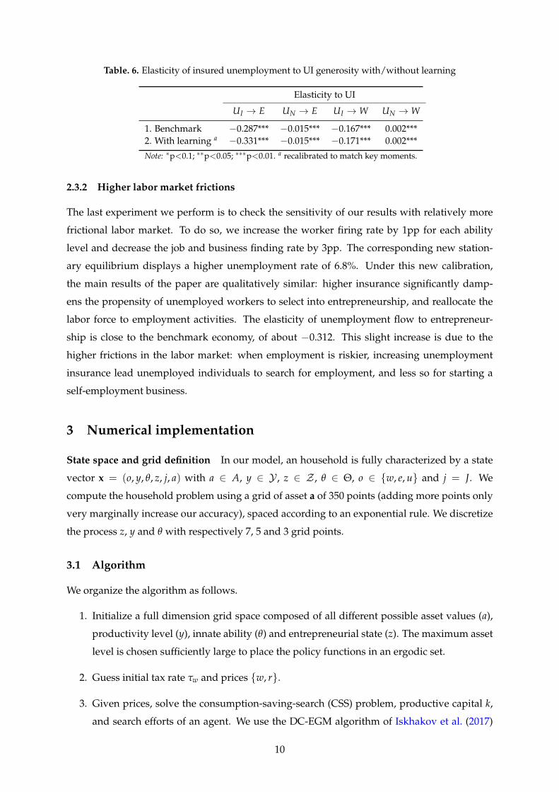
Table. 6. Elasticity of insured unemployment to UI generosity with/without learning

Elasticity to UI

UI ! E UN ! E UI ! W UN ! W

1. Benchmark �0.287*** �0.015*** �0.167*** 0.002***2. With learning a

�0.331*** �0.015*** �0.171*** 0.002***Note: ⇤p<0.1; ⇤⇤p<0.05; ⇤⇤⇤p<0.01. a recalibrated to match key moments.

2.3.2 Higher labor market frictions

The last experiment we perform is to check the sensitivity of our results with relatively more

frictional labor market. To do so, we increase the worker firing rate by 1pp for each ability

level and decrease the job and business finding rate by 3pp. The corresponding new station-

ary equilibrium displays a higher unemployment rate of 6.8%. Under this new calibration,

the main results of the paper are qualitatively similar: higher insurance significantly damp-

ens the propensity of unemployed workers to select into entrepreneurship, and reallocate the

labor force to employment activities. The elasticity of unemployment flow to entrepreneur-

ship is close to the benchmark economy, of about �0.312. This slight increase is due to the

higher frictions in the labor market: when employment is riskier, increasing unemployment

insurance lead unemployed individuals to search for employment, and less so for starting a

self-employment business.

3 Numerical implementation

State space and grid definition In our model, an household is fully characterized by a state

vector x = (o, y, q, z, j, a) with a 2 A, y 2 Y , z 2 Z , q 2 Q, o 2 {w, e, u} and j = J. We

compute the household problem using a grid of asset a of 350 points (adding more points only

very marginally increase our accuracy), spaced according to an exponential rule. We discretize

the process z, y and q with respectively 7, 5 and 3 grid points.

3.1 Algorithm

We organize the algorithm as follows.

1. Initialize a full dimension grid space composed of all different possible asset values (a),

productivity level (y), innate ability (q) and entrepreneurial state (z). The maximum asset

level is chosen sufficiently large to place the policy functions in an ergodic set.

2. Guess initial tax rate tw and prices {w, r}.

3. Given prices, solve the consumption-saving-search (CSS) problem, productive capital k,

and search efforts of an agent. We use the DC-EGM algorithm of Iskhakov et al. (2017)

10

for the CSS problem.

4. Construct the transition matrix M generated by Py, Pz and Pq , a0(x), sw(x), se(x). Com-

pute the associated stationary measure of individuals G(x), by first guessing an initial

mass of one of households with zero asset and then by iterating on G0(x) = MG(x) until

|G0(x)� G(x)| < µ, with µ very small.

5. Compute the resulting total asset level, total labor supplied and total investment in the

entrepreneurial sector. Total capital invested in the corporate sector is given as the differ-

ence between total savings and total capital invested in the entrepreneurial sector. Total

labor used in the corporate sector is given by total labor supplied by workers.

6. Update prices {r, w} using the marginal productivities in the corporate sector and tax rate

tw to close the government budget up to a relaxation. Back to step 2 until convergence of

labor income tax rate and prices.

3.2 Transitional dynamics

To solve the transition, we compute the solutions of the household problem backward, starting

at the new steady-state. We then find prices that are consistent with the implied policies and we

iterate until convergence. We assume that the economy is in the initial steady-state in period 0

and the reform is announced and implemented in period 1. Agents did not anticipate the policy

before its implementation. The economy makes a transition to reach the final steady-state in

period T. We choose T large enough so that the resulting stationary distribution in period T is

close enough to the final steady-state equilibrium. The algorithm for the transition dynamics

is:

1. Guess a path for {L1, ...,LT�1} with Lt = {rt, wt, tw,t}. L0 and LT are given by initial and

final steady-states.

2. Use value functions of the final steady-state (period T) to solve the households’ problem

backward starting from T � 1 until period 1.

3. Use the distribution of the initial steady-state and the resulting policy functions to com-

pute the path of the distribution of household {G(x)1, ..., G(x)T}.

4. Given these distributions, compute new path {L1, ...,LT�1}. Iterate from step 2 until the

difference between the initial path is close enough to the resulting path.

5. When convergence is achieved, check if the resulting final distribution G(x)T is close

enough to the steady-state distribution G(x)T up to a relaxation. If the two distributions

are identical, then stop, else, increase the number of periods T.

11

3.3 Additional figures

Figure 2. Model flows from insured unemployment to entrepreneurship.

UI = 26w, θ = θ2 UI = 99w, θ = θ2 UI = 26w, θ = θ0 UI = 26w, θ = θ0

0.0e+00

5.0e−06

1.0e−05

1.5e−05

2.0e−05

0 10 20 30 40 50wealth

Flow

Ui t

o W

0e+00

5e−07

1e−06

0 10 20 30 40 50wealth

Flow

Ui t

o E

Note: we display the flows out of insured unemployment with j = J for two models with the same benchmarkinitial distribution: the baseline with J = 26 weeks (solid line) and an alternative with J = 99 weeks (dashed line).

Figure 3. Effect of alternative tax scheme on occupation masses.

Model baseline alternative tax 1.0/0.0 alternative tax 0.5/1.0

0.84

0.85

0.86

0.87

8.5 9.0 9.5 10.0 10.5log(UI max)

Paid

em

ploy

men

t rat

e

0.050

0.055

0.060

0.065

8.5 9.0 9.5 10.0 10.5log(UI max)

Une

mpl

oym

ent r

ate

0.07

0.08

0.09

0.10

8.5 9.0 9.5 10.0 10.5log(UI max)

Entre

pren

eurs

hip

rate

12

References

Cagetti, M., De Nardi, M., 2006. Entrepreneurship, Frictions, and Wealth. Journal of Political Economy

114, 835–870.

Clementi, G.L., Palazzo, B., 2016. Entry, exit, firm dynamics, and aggregate fluctuations. American

Economic Journal: Macroeconomics 8, 1–41.

Farber, H.S., Rothstein, J., Valletta, R.G., 2015. The effect of extended unemployment insurance benefits:

Evidence from the 2012-2013 phase-out. American Economic Review 105, 171–76.

Hsu, J.W., Matsa, D.A., Melzer, B.T., 2018. Unemployment insurance as a housing market stabilizer.

American Economic Review 108, 49–81.

Iskhakov, F., Jørgensen, T.H., Rust, J., Schjerning, B., 2017. The endogenous grid method for discrete-

continuous dynamic choice models with (or without) taste shocks. Quantitative Economics 8, 317–

365.

Koellinger, P., Minniti, M., 2009. Unemployment benefits crowd out nascent entrepreneurial activity.

Economics Letters 103, 96–98.

13