Preliminary Draft

Does Cash-in-Hand Matter?New Evidence from the Labor Market

September 2006�

David Card Raj Chetty Andrea WeberUC-Berkeley UC-Berkeley IAS-Viennaand NBER and NBER and UC-Berkeley

ABSTRACT

This paper provides new evidence on the e¤ects of cash-in-hand on household be-havior. Using sharp discontinuities in eligibility for severance pay and extended unem-ployment bene�ts in Austria, combined with data on over one-half million job losers,we reach three main �ndings: (1) a lump-sum severance payment equal to two monthsof wages lowers the rate of new job �nding by 8-12% on average; (2) an extension of thepotential duration of UI bene�ts from 20 weeks to 30 weeks lowers job-�nding rates inthe �rst 20 weeks by 6-10%; and (3) the increases in the duration of job search inducedby both programs have no e¤ect on job match quality, as measured by wages or theduration of the next job. We use a job search model to show how these estimatescan distinguish between commonly used dynamic models of household behavior, anddevelop a metric that can be used to calibrate such models to match our empirical �nd-ings. Our empirical �ndings are inconsistent with a simple permanent income model aswell as �rule-of-thumb�models with a myopic agent. The results favor a model whereagents are forward-looking yet have limited ability to smooth consumption.

�We are extremely grateful to Rudolph Winter-Ebmer and Jospeh Zweimuller for assistance in obtaining thedata used in this study. Thanks to Joe Altonji, David Autor, Richard Blundell, Peter Diamond, Caroline Hoxby,David Lee, David Romer, Emmanuel Saez, Robert Shimer, and numerous seminar participants for comments andsuggestions. Matthew Grandy provided excellent research assistance. Funding was provided by the Center for LaborEconomics at UC Berkeley.

I Introduction

Does disposable income (�cash-in-hand�) a¤ect household behavior? The answer to this basic

question has implications for a range of economic issues. In macroeconomics, the answer distin-

guishes between a set of widely used models of household behavior, ranging from the benchmark

permanent income hypothesis with complete markets (where changes in disposable income have

small e¤ects on consumption) to �rule of thumb�models (where consumption rises dollar-for-dollar

with income). In public �nance, the answer is relevant for optimal tax and social insurance poli-

cies. Temporary tax cuts can only be e¤ective as a �scal stimulus if households are sensitive to

cash-in-hand. Similarly, the bene�ts of temporary income support programs such as unemployment

insurance and welfare are determined by the extent to which individuals can smooth short-term

income �uctuations on their own (Baily 1978, Chetty 2006a).

The e¤ects of cash-in-hand have been studied for several decades in the macroeconomics liter-

ature, where researchers have estimated the e¤ect of windfall cash grants such as tax rebates on

non-durable household consumption (see section II for a brief summary of this literature). However,

there is still no �rm consensus on whether individuals can smooth intertemporally, are fully cash

constrained, or fall somewhere in between.1

In this paper, we provide new evidence on the e¤ects of cash-in-hand from the labor market. In

particular, we study whether lump-sum severance payments and unemployment bene�t extensions

for job losers in Austria a¤ect search behavior and subsequent job outcomes. Conceptually, our

analysis is analogous to existing studies, and simply uses a di¤erent measure of �consumption�

(labor/leisure instead of goods). Excess sensitivity of labor supply to cash-in-hand distinguishes

between the permanent income hypothesis (PIH) and other dynamic models in the same way as

excess sensitivity of consumption. Indeed, we show that the e¤ects of cash-in-hand on consumption

can be inferred from our estimates of the labor supply responses using a simple job search model.

Our labor market approach is a useful complement to existing consumption-based studies for

three reasons. First, eligibility for severance pay in Austria is based on a simple discontinuous rule

that applies to all private sector workers outside the construction sector: people with over 3 years

of job tenure are eligible, whereas those with shorter tenures are not. In addition, administrative

wage and daily employment data are available for the universe of private sector workers, giving us

a sample of 650,000 job losers. The sharp discontinuity and large sample allow us to obtain more

1The lack of consensus is underscored in the review by Browning and Lusardi (1996), who note that they personallydisagree on importance of liquidity constraints.

1

precise estimates of the e¤ects of cash-in-hand than consumption-based studies, which are often

limited by small sample sizes and noise in consumption measures. Second, the severance payment

is generous � equivalent to two months of pre-tax salary, or 3,300 Euros at the sample median.

This makes our analysis less subject to Browning and Crossley�s (2001) criticism that the welfare

cost of failing to smooth over small amounts (e.g. the $300-$600 tax rebates in Johnson, Parker,

and Souleles 2006) is negligible. Third, the panel structure of our data allows us to examine the

long-term e¤ects of cash grants, in particular subsequent job quality. This allows us to further

distinguish between dynamic models of search behavior and provide new evidence on subsequent

job quality e¤ects, an issue of independent interest in the literature on job search.

We exploit the quasi-experiment created by the discontinuous Austrian severance pay law using

a regression discontinuity (RD) design, essentially comparing the search behavior of individuals laid

o¤ just before and after the 36 month cuto¤ for eligibility. The key threat to a causal interpretation

of our estimates is that �rms may manipulate their �ring decisions to avoid paying severance,

leading to non-random selection around the discontinuity and invaliding the �experiment.� We

evaluate this possibility by comparing the number of layo¤s at each level of job tenure, and by

examining the characteristics of job losers with just under and just over 3 years of tenure. We

�nd no systematic evidence of selection on observables around the discontinuity � a result that

is consistent with relatively restrictive �ring regulations in Austria and laws against the strategic

timing of layo¤s.2 This suggests that any discontinuities in search behavior around the 36 month

cuto¤ can be attributed to the causal e¤ect of severance pay.

Our empirical analysis leads to three main �ndings. First, lump sum severance pay has a clearly

discernible and economically signi�cant e¤ect on the duration of unemployment and time to re-

employment. The hazard rate of �nding a new job during the �rst 20 weeks of the unemployment

spell (the period of eligibility for regular UI bene�ts in Austria) is 8-12% percent lower for those

who are just barely eligible for severance pay than for those who are just barely ineligible. Second,

using a parallel analysis of a discontinuity in the UI bene�t system, we �nd that job seekers who are

eligible for 10 extra weeks of unemployment bene�ts exhibit 6-10% lower rates of job �nding during

the �rst 20 weeks of search. This result shows that individuals anticipate the longer duration of

bene�ts and accordingly reduce search e¤ort before the bene�t extension takes e¤ect. Hence, this

�nding provides strong evidence of forward looking behavior, inconsistent with a �rule of thumb�

2As we discuss in more detail in Section IV, the Austrian labor market is characterized by relatively high ratesof job mobility and low unemployment (an average rate of 4.8% over the 1992-2002 period). Nevertheless, �rms facesigni�cant regulations governing layo¤s. See Winter-Ebmer (2002).

2

model where agents are completely myopic.

Third, we �nd that neither lump sum severance payments nor extended bene�ts have any e¤ect

on the �quality�of subsequent jobs. Mean wages, the duration of subsequent jobs, occupational

mobility, and other measures of job match outcomes are essentially una¤ected by eligibility for

severance pay or extended bene�ts. An advantage of our results relative to prior studies of match

quality is that our estimates are su¢ ciently precise to rule out fairly small match quality gains. For

example, the additional search induced by the severance payment or bene�t extension is estimated

to raise the mean subsequent wage by less than 1% at the upper bound of the 95% con�dence

interval. Thus, severance pay and extended bene�ts appear to extend durations primarily through

the margin of search intensity rather than through a shift in the reservation wages of job seekers.

Combining these �ndings with predictions from a job search model that nests a range of models

(from the PIH to complete myopia), we test between various commonly used dynamic models of

household behavior. We �rst show that two widely applied benchmark cases �a simple version

of the PIH where agents smooth relative to permanent income and a credit-constrained model

where agents set consumption equal to income � are rejected with p<0.001. We then develop

a simple metric to characterize the types of models that can match the data. Our estimates

suggest that deviations from the PIH are substantial: a typical job searcher behaves as if they

are roughly halfway between the PIH and fully credit-constrained benchmarks. We conclude that

models such as bu¤er-stock behavior with variable job search intensity, incomplete consumption

smoothing, and a forward-looking agent �t the data. This �nding implies that temporary income

support and tax rebate policies can have substantial economic e¤ects. Perhaps more importantly,

the estimated moment can be easily matched when calibrating dynamic models to analyze such

policies in subsequent work.

The remainder of the paper proceeds as follows. Section II discusses related literature. Section

III presents our theoretical model. Section IV describes the institutional background and data.

Section V outlines our estimation strategy and identi�cation assumptions. Section VI presents the

empirical results on unemployment durations, and Section VII presents results on search outcomes.

Section VIII uses the empirical estimates to calibrate the model. Section IX concludes.

3

II Related Literature

Our analysis builds on insights and methods from several literatures in macroeconomics, labor

economics, and public �nance. The �rst is a set of studies that measures the e¤ects of transitory

income shocks on consumption.3 Bodkin (1959) and Bird and Bodkin (1965) estimated that house-

holds spent 40-70% of a one-time windfall payment issued to World War II veterans in the year of

the rebate on nondurable consumption.4 Subsequent studies of tax rebates using aggregate data

(e.g., Blinder, 1981; Blinder and Deaton, 1985) also found relatively large impacts on nondurable

consumption in the quarter of receipt. More recent microdata-based studies of pre-announced tax

cuts and rebates include Parker (1999) and Souleles (1999), both of which �nd that current non-

durable spending absorbs 30-65 percent of the change in after-tax current income. In contrast,

however, Hsieh (2003) �nds no relation between spending and the timing of recurring payments

to Alaska residents from the Alaska State fund. Finally, Johnson, Parker, and Souleles (2006)

analyze the 2001 federal tax rebates, exploiting the fact that checks were mailed at di¤erent dates

to di¤erent families. They report estimates of the e¤ect on non-durable consumption in the quarter

of the rebate (relative to the preceding quarter) centering on 35-40 cents per dollar.

A second related literature focuses on estimating consumption-income sensitivity for unem-

ployed individuals using variation in unemployment bene�ts. Gruber (1997) relates the change in

food consumption for families with a recently unemployed head to the generosity of the UI bene�ts

potentially available to the head. He estimates that a 10% increase in the UI bene�t level leads to

a 2.5-3.3 percent increase in food consumption by the unemployed. Subsequent analyses conducted

by Browning and Crossley (1999) and Bloemen and Stancanelli (2005) on samples of longer-term

job losers in Canada and the U.K. �nd smaller e¤ects of UI bene�ts on total expenditures in the ag-

gregate, but larger e¤ects among job losers with low assets prior to job loss. Interestingly, Bloemen

and Stancanelli report that job losers who received a severance bene�t have higher consumption

while unemployed, a result consistent with our �ndings below.

3Many other strands of the micro consumption literature are also related, including the tests for liquidity con-straints developed by Zeldes (1989), and the �excess sensitivity�results in Hall and Mishkin (1982) and Altonji andSiow (1987). See Deaton (1992) for a summary and thoughtful interpretation of much of the literature up the early1990s, and Browning and Lusardi (1996) for a more recent survey.

4The payment was based on an actuarial adjustment to the life insurance provided to all veterans, and averaged$175. A key feature of the rebate was that it was unexpected - according to Bodkin the payments were announced inNovember 1949 and mailed in the �rst few months of 1950. In a benchmark permanent income model, the predictede¤ect of a transitory income shock on current non-durable consumption is roughly proportional to the discount rate(e.g., 5-10%). Carroll (2001) has argued against the relevance of this benchmark and in favor of a model withprecautionary savings that suggests a larger e¤ect. Both the benchmark model and Carroll�s alternative imply anegligible e¤ect of an anticipated income shock on the change in consumption.

4

Outside the consumption literature, our analysis is closely related to studies of the e¤ects of

unemployment bene�ts and assets on job search e¤ort and the duration of unemployment. On the

theoretical side, conventional job search models imply that higher unemployment bene�ts and longer

potential eligibility for bene�ts will raise the average duration of unemployment (e.g., Mortensen,

1977; Mortensen, 1986). Most search models assume risk neutrality and ignore savings, and thus

do not study wealth e¤ects. However, a few studies have incorporated these features and show

that under certain conditions increases in wealth lower search intensity (Danforth, 1979; Lentz

and Tranaes, 2001). On the empirical side, a number of well-known studies have shown that the

duration of unemployment is a¤ected by the generosity and potential duration of UI bene�ts (e.g.,

Meyer, 1990; Katz and Meyer, 1990; Lalive and Zweimuller, 2004). These studies have generally

assumed that the entire response of search behavior to UI bene�ts is due to moral hazard (a

substitution e¤ect) rather than wealth e¤ects. Chetty (2006b) points out that the wealth e¤ects of

UI bene�ts may be non-trivial when agents have limited liquidity. He decomposes the UI bene�t

elasticity into a wealth e¤ect and substitution e¤ect by examining the heterogeneity of duration-

bene�t elasticities across liquidity constrained and unconstrained groups in the U.S. He �nds that

a substantial portion of the UI bene�t e¤ect is a wealth e¤ect, consistent with our results here.

The key advantages of the present study relative to the existing literature are the isolation of a

credibly exogenous source of variation in wealth and the use of this variation to distinguish between

dynamic models of household behavior.

Our analysis also contributes to the literature on match quality gains from job search. Ehrenberg

and Oaxaca (1976) found that increases in UI bene�ts led to small increases in wages at the next

job. Subsequent studies have found mixed, fragile results; see Burtless (1990) and Cox and Oaxaca

(1990) for reviews and Addison and Blackburn (2000) and Centeno (2004) for more recent analysis.

This literature remains quite controversial largely because of the lack of compelling variation in

bene�t policies. Our analysis yields substantially more precise estimates of match quality gains

than earlier studies because of the large sample and RD research design.

Finally, our study is related to the extensive literature on optimal social insurance (e.g. Baily

1978, Flemming 1978, Hansen and Imrohoroglu 1992, Wang and Williamson 1996, Chetty 2006a,

Shimer and Werning 2006). Although we do not explicitly consider an optimal social insurance

problem here, our �ndings bear on the problem by empirically identifying the extent to which

households can smooth consumption, a central parameter in these calculations. Our �ndings can

be applied in subsequent studies of optimal social insurance by calibrating models to match the

5

moments estimated below.

III A Job Search Model

We begin our analysis by presenting a simple job search model that provides a structural framework

for interpreting our empirical �ndings. The model we analyze nests a range of dynamic models

commonly used in the literatures on consumption and search, such as the standard permanent

income model, bu¤er stock models, and �rule of thumb�behavior where the agent is myopic and

sets consumption equal to income. We use the model for two purposes. First, we derive a set of

comparative statics predictions on the e¤ect of assets and UI bene�ts on search behavior to test

between certain benchmark models. Second, we construct a metric based on the relative e¤ects of

severance pay and bene�t extensions that can be used in calibrating models to match the data.

Model Setup. The model is closely based on Lentz and Tranaes (2004), who incorporate

intertemporal consumption and savings decisions into a standard job search model. Consider a

discrete-time setting where an individual has a �nite planning horizon and a subjective rate of time

discounting of �. Let r denote the �xed interest rate in the economy. Suppose the individual enters

period t unemployed. He can control his unemployment duration only by varying his level of search

intensity, st. The agent chooses search intensity at the beginning of period t, and immediately

learns if he has obtained a job (which starts in period t itself). Normalize st to equal the probability

of �nding a job in the current period. The disutility of supplying st units of search e¤ort is given

by a strictly convex function (st).

If the agent is successful in job search and �nds a new job, he earns a �xed real wage w

inde�nitely and faces no further uncertainty. For simplicity, we ignore any variability in wage

o¤ers, eliminating reservation-wage choices. We discuss how relaxing this assumption would a¤ect

our results below.

Let cet denote the employed agent�s consumption in period t if job search is successful in that

period. If the agent fails to �nd a job in period t, he receives an unemployment bene�t bt and sets

consumption to cut . The agent then enters period t+1 unemployed, when he chooses search e¤ort

st+1 and the problem repeats.

The agent has a within-period utility over consumption (ct) given by a strictly concave function

u(ct). To allow for borrowing constraints, assume there is a lower bound L on assets which may

or may not be binding.

6

The value function for an individual who �nds a job at the beginning of period t, conditional

on beginning the period with assets At is

Vt(At) = maxAt+1�L

u(At �At+1=(1 + r) + w) +1

1 + �Vt+1(At+1). (1)

The value function for an individual who fails to �nd a job at the beginning of period t and remains

unemployed is:

Ut(At) = maxAt+1�L

u(At �At+1=(1 + r) + bt) +1

1 + rJ(At+1) (2)

where J(At+1) is the value of entering the next period unemployed. It is easy to show that Vt is

concave because the agent faces a deterministic pie-eating problem once re-employed. The function

Ut, however, can be convex. Lentz and Tranaes (2004) address this problem by introducing a

wealth lottery that can be played prior to the choice of search intensity whenever U is non-concave,

although they note that in simulations of the model, non-concavity never arises. We shall simply

assume that U is concave.

The agent chooses st to maximize expected utility at the beginning of period t, taking into

account the cost of search:

J(At) = maxst

stVt(At) + (1� st)Ut(At)� (st) (3)

The �rst order condition for optimal search intensity is

0(s�t ) = Vt(At)� Ut(At) (4)

re�ecting the fact that the agent chooses st to equate the marginal cost of search e¤ort with the

marginal value of search e¤ort, which is given by the di¤erence between the optimized values of

employment and unemployment.

Our testable predictions and empirical analysis all follow from the comparative statics of equa-

tion (4). First consider the e¤ect of the UI bene�t level on search e¤ort. Di¤erentiating equation

(4) and using the envelope theorem, we obtain:

@s�t =@bt = �u0(cut )= 00(s�t ) < 0 (5)

Equation (5) is the standard result that higher unemployment bene�ts reduce search e¤ort, thereby

7

extending unemployment durations. This prediction does not distinguish between dynamic models

of household behavior, because higher unemployment bene�ts increase durations regardless of the

degree of intertemporal consumption smoothing. Consistent with this result, many well-known

studies have found that increases in UI bene�ts raise the duration of joblessness. To distinguish

between the models of interest, we therefore turn to other comparative static implications of (4).

Prediction 1: Severance Pay. The e¤ect of an exogenous cash grant, such as a severance pay-

ment, on search e¤ort is given by:

@s�t =@At = fu0(cet )� u0(cut )g= 00(s�t ) � 0 (6)

Equation (6) shows that the e¤ect of a cash grant on search intensity is determined by the gap in

marginal utilities between employed and unemployed states, which is proportional to the size of

consumption drop cet � cut . Intuitively, when consumption is smooth across states, a cash grant

increases the value of being employed and unemployed by a similar amount, and thus does not

a¤ect search behavior much. In contrast, if consumption is substantially lower when unemployed,

the cash grant raises the value of being unemployed relative to the value of being employed, leading

to a reduction in search e¤ort

It is well known that if an agent has access to complete state-contingent insurance markets (full

insurance), cut = cet . A PIH model with complete markets therefore predicts that @s�t =@At = 0.

In this extreme case, a lump sum severance payment has no e¤ect on search behavior, a prediction

that we test in our empirical analysis. More generally, if cut is close to cet , as would be expected

if individuals can freely borrow and have a high probability of �nding a job relatively quickly, the

asset e¤ect is small. In contrast, if individuals face asset constraints or have to consume only

their net income while unemployed, the asset e¤ect will be relatively large. Thus, there is a

direct connection between the degree of consumption smoothing achieved by job searchers and the

responsiveness of search intensity to an increase in wealth.

An estimate of @s�t =@At is also useful in assessing the degree of moral hazard caused by tem-

porary income support programs, as shown by Chetty (2006b). To see this in our model, note

that:

@s�t =@wt = u0(cet )= 00(s�t ) > 0

and hence

@s�t =@bt = @s�t =@At � @s�t =@wt (7)

8

Equation (7) shows that the response of search intensity to an increase in unemployment bene�ts

can be written as the sum of a wealth e¤ect and a price (or substitution) e¤ect The former has no

direct e¢ ciency costs, whereas the latter represents a �moral hazard�response to the price distortion

induced by subsidizing unemployment. Many empirical studies of unemployment insurance ignore

the asset e¤ect by assuming that unemployment durations depend on the ratio of bene�ts to wages.

These studies implicitly assume that the PIH with complete markets model applies. To the extent

that job seekers have lower consumption when unemployed, however, one should expect bene�ts to

have a larger impact (in absolute value) than wages.5

Prediction 2: Extended Bene�ts. Next, we examine how search intensity in period t is a¤ected

by the level of future bene�ts, bt+1. Using equations (3) and (2) we obtain:

@s�t =@bt+1 = �Et[(1� s�t+1)u0(cut+1)]=[(1 + �) 00(s�t )] � 0 (8)

This equation implies that a rise in the future bene�t rate lowers search intensity in the current

period, but only by the discounted value of those bene�ts, which depends on (1� s�t+1) and 1 + �.

A completely myopic �rule of thumb�agent places no value on the future and has � = 1. The

complete myopia model therefore predicts that @s�t =@bt+1 = 0. In this model, extending the

potential duration of UI bene�ts has no e¤ect on search behavior prior to the extension, which is

the second prediction that we test in our empirical analysis. More generally, the e¤ect of the bene�t

extension on pre-extension search behavior provides a measure of how forward-looking agents are:

agents who place more weight on the future respond more to bene�t extensions.

Prediction 3: Search Outcomes. A �nal prediction that is useful in distinguishing between

models of search behavior is the e¤ect of an increase in assets or future unemployment bene�ts on

subsequent job quality. This prediction cannot be derived from the model here because we have

assumed that wages are �xed and agents only control search intensity. However, in a more general

model with a non-degenerate distribution of wages or job qualities, one would expect an increase in

assets or future bene�ts to lead to a rise in the quality of the next job (Danforth, 1979; Mortensen,

1977).

Table 1 summarizes these three predictions and shows how they distinguish between four po-

tential models of household behavior.5 Interestingly, this pattern is present in the well-known study by Meyer (1990), whose estimates imply that the

e¤ect of UI bene�ts on the hazard rate of leaving unemployment is about 1.8 times larger than the e¤ect of weeklyearnings.

9

A Metric for Calibration. Combining equations (6) and (8), we obtain a simple metric that

can be used to quantitatively identify the class of models that �t the data. In particular, consider

the ratio of the e¤ect of a 1 euro increase in assets and a 1 euro increase in the value of future

bene�ts on search e¤ort: em =@s�t =@At@s�t =@bt+1

= D � 1 + �

1� s�t+1(9)

where

D =u0(cut )� u0(cet )Et[u0(cut+1)]

:

The moment em can be easily simulated in dynamic models of household behavior because it requires

knowledge only of the utility function and consumption drop ( ce�cuce) caused by unemployment. In

particular, the function can be left unspeci�ed, permitting a calibration that is relatively robust

to the way in which the the search process is modelled. The empirical value of em can be obtained

from the ratio of the severance pay and bene�t extension e¤ects estimated in our empirical analysis.

Figure 1 illustrates the idea underlying the calibration by ordering a set of models on a contin-

uum by their implied value of em. The models on the left side of the continuum assume a higher

degree of intertemporal smoothing by households, and thus predict a lower sensitivity of search

behavior to cash-in-hand. At the left extreme of the continuum is the full insurance model, where

consumption is perfectly smooth across states and time, and temporary income shocks have no

e¤ect on behavior, implying D = em = 0. At the right extreme is a �complete myopia�model

where households do not smooth intertemporally at all, and simply set current consumption equal

to current income. In this model, severance pay a¤ects search e¤ort substantially but bene�t

extensions have no e¤ect, implying em = 1. The interior of the continuum includes models that

have intermediate values of em 2 (0;1), such as the simple permanent income hypothesis without

complete markets, bu¤er stock models (Deaton 1991; Carroll 1992), and credit-constrained models

where agents are forward looking but face a binding asset constraint.

In section VIII, we calibrate em for some benchmark models and compare these numbers with the

corresponding value estimated from the data. This exercise can be viewed as a means of identifying

the �location� of the representative household in the data on the continuum in Figure 1. More

precisely, em identi�es a plane within the space of parameters de�ned by preferences and �nancial

technologies (e.g. the asset limit, insurance market completeness, discount rate, risk aversion). Of

course, a single moment is insu¢ cient to pin down all of these parameters, but it does turn out

to be su¢ cient to distinguish between certain benchmark cases. The value of em is also of direct

10

interest for assessing the optimal level of unemployment insurance, since D is a su¢ cient statistic

for determining the marginal bene�ts of social insurance in a general class of dynamic models

(Chetty 2006a).

IV Institutional Background and Data

The Austrian labor market is characterized by an unusual combination of institutional regulation

and labor market �exibility. Virtually all private sector jobs are covered by collective bargaining

agreements, negotiated by unions and employer associations at the industry level (EIRO, 2006).

Firms are also required to consult with their works councils in the event of a layo¤ and to give

at least 6 weeks notice of a pending mass layo¤ (Winter-Ebmer 2002). Despite these features,

rates of job turnover and overall employment are relatively high, whereas unemployment is low.

Winter-Ebmer (2002), for example, shows that rates of �job creation�and �job destruction�for the

overall economy and for most sectors are comparable to those in the U.S. The overall employment-

population rate of 15-64 year olds during the 1990s averaged 68% - higher than in Germany or

France but below the rates in the U.K. or the U.S. However, rates of employment for younger

workers are higher and are comparable to the U.S.6 The average unemployment rate over the

1993-2004 period was among the lowest in Europe at 4.1%.

A key aspect of the �ring regulations in Austria is severance pay, which was introduced for white

collar workers in 1921 and was expanded to include all other workers in 1979. Severance payments

are made by �rms according to a �xed schedule legislated by the government. In particular,

workers outside of the construction industry who are laid o¤ after 3 years of service must be given

a severance payment equal to 2 months of their previous salary.7 Payments are generally made

within one month of the job termination, and are not taxable.

Job losers with su¢ cient work history are also eligible for unemployment bene�ts. Speci�-

cally, individuals who have worked for 12 months or more over the past two years can receive a

unemployment bene�t (UI) that replaces approximately 55% of their prior net wage, subject to a

minimum and maximum (though only a small fraction of individuals are at maximum). Workers

who are laid o¤ by their employer are immediately eligible for bene�ts, while those who quit (or are

6Austria has among the lowest employment rates in Europe for people over 55: 42% for people age 55-59 and only12% for those 60-64 (EIRO, 2005).

7The severance amount rises to 3 months of pay for workers with 5 years of service, 4 months after 10 years, andup to 12 months after 25 years of service. Employees who quit or are �red for cause are not eligible for severancepay. Workers in the construction industry are covered by a di¤erent law. The law governing severance pay waschanged in January 2003 (outside our dataset).

11

�red for cause) have a four week waiting period. The maximum duration of regular unemployment

bene�ts is a discontinuous function of the total number of months that the individual worked (at

any �rm) within the past �ve years. Individuals with less than 36 months of previous employment

receive 20 weeks of bene�ts, while those who have worked for 36 months or more receive 30 weeks of

bene�ts (which we term �extended bene�ts�). Job losers who exhaust their regular unemployment

bene�ts can move to a means-tested secondary bene�t, known as �unemployment assistance,�(UA)

which pays a lower level of bene�ts inde�nitely. Importantly, however, UA bene�ts are reduced

euro-for-euro by the amount of any other family income. As a result, the average UA replacement

rate is 38% of the UI bene�t level in the population.8

Our empirical analysis exploits the discontinuities in the severance pay and bene�t duration

laws to identify the causal e¤ects of these two entitlements on the duration of unemployment and

the time to a new job. The e¤ects of the two policies can be independently identi�ed because

they are discontinuous functions of di¤erent running variables: previous job tenure in the case of

severance pay, and previous weeks of work in the case of extended bene�ts for regular UI Nev-

ertheless, there is a subset of individuals �those who did not work in the two years prior to the

current job �for whom the severance pay and extended UI bene�t discontinuities overlap. This

creates a �double discontinuity� that complicates the empirical analysis relative to the standard

regression discontinuity design proposed by Thistlewaite and Campbell (1960), where there is only

one discontinuous policy change.

Figure 2a illustrates the problem by plotting the fraction of individuals in our data who receive

an extended unemployment bene�t (EB) as a function of months of job tenure. Individuals

who have 36 or more months of job tenure necessarily have worked for more than 3 of the last 5

years; hence the fraction receiving EB is 100% on the right side of the severance pay discontinuity.

Individuals who have 35 months of job tenure receive EB if they worked for one month or more at

another �rm within the past �ve years. Since only 80% of individuals laid o¤ with 35 months of

job tenure satisfy this condition, there is a 20 percentage point jump the fraction receiving EB at

36 months of job tenure. Consequently, any discontinuous change in behavior at 36 months of job

tenure is mainly due to severance pay, but includes a small (20 percentage point) e¤ect of extended

bene�ts. A similar double discontinuity arises at the threshold for EB, as shown in Figure 2b.

The fraction of individuals receiving severance pay jumps discontinuously by approximately 20%

at 36 months worked. Hence changes in behavior around 36 months worked are likely to be caused

8See section VIII for details on this computation.

12

primarily by EB, but could also be partly attributed to severance pay. We account for the double

discontinuity in our empirical analysis using two independent methods described below.

IV.A Data and Sample De�nition

We use data from the Austrian social security registry, which covers the universe of private sec-

tor employees, spanning 1980-2001. The dataset includes daily information on employment and

registered unemployment status, total wages received from each employer in a calendar year, and

information on workers� and �rms� characteristics (e.g. age, education, gender, marital status,

industry, and �rm size).

We do not have any information on actual severance payments, or the amount of UI bene�ts paid

in this dataset. Hence, we cannot construct ��rst stage�estimates of the e¤ect of the discontinuous

policies on actual payments received. Compliance with the severance pay law is believed to be

nearly universal, in part because of the monitoring e¤ort of works councils and legal penalties for

violations (CESifo 2004; Baker and Tilly 2005). Given our data source, we also believe we have

accurately captured the eligibility rules for extended bene�ts. Consequently, we believe that the

eligibility rules for both severance pay and EB�s create so-called �sharp� regression discontinuity

designs, where the fraction eligible jumps from 0 to 1 at the discontinuity (Hahn, Todd, and van

der Klaauw 2001).

We make four restrictions on the original data to arrive at our primarily analysis sample. First,

we include only non-construction workers between the ages of 20 and 50 at the time of the job

termination, to avoid complications with the retirement system and the di¤erential treatment of

construction workers. Second, we include only individuals who take up UI bene�ts within 28 days

of job loss, thereby eliminating voluntary quitters (who are ineligible for severance pay and have a

28 day waiting period for UI eligibility). Third, we focus on individuals around the discontinuities

of interest by only including individuals who worked at their previous �rm for between 1 and 5 years,

and who worked between 1 and 5 years of the past 5 years. Consequently, everyone in the sample

is eligible for UI bene�ts (though not all are eligible for extended bene�ts), and everyone in the

sample is eligible for either 2 months of severance pay, or none. Finally, we drop individuals who

were recalled to their prior �rm in order to eliminate temporary layo¤s who may not be searching

for a job. These restrictions leave us with a sample of 650,922 unemployment spells.

Table 2 shows summary statistics for the full sample. Sixty percent of the sample has additional

schooling beyond the compulsory level � most members of this group have an apprenticeship,

13

equivalent to a �some college� level of education in the U.S. Only 44 percent of the sample are

married, re�ecting relatively the relatively low age of the sample and the prevalence of non-marital

cohabitation in Austria.9 Owing to our sample requirement that people have worked between

1 and 5 years at their last job, average tenure is relatively short (26.5 months). However, most

people have worked at other jobs in the past 5 years: the mean numbers of months worked is 41.2.

Roughly one-�fth of the sample is eligible for severance pay, while 66% are eligible for extended UI

bene�ts. The mean wage is 17,034 Euros per year in year 2000 Euros. Wages are top-coded at

the social security tax cap in the dataset. This cap binds for very few individuals in our sample:

less than 2% of the observations have censored wages.

There are two measures of unemployment durations that can be constructed in the data. The

�rst is the total number of days that an individual is registered with the unemployment agency.

Individuals are required to register while they are receiving bene�ts, and can remain registered

even when their bene�ts are exhausted in order to take advantage of job training and job search

assistance services o¤ered by the agency. This measure corresponds to the o¢ cial de�nition

of �unemployment� in government statistics, and we therefore refer to it below simply as the

individual�s �unemployment duration.� Only a small fraction (0.5 percent) of people in the sample

have censored spells of unemployment; the summary statistics in Table 2 ignore this issue. Spells

of registered unemployment are relatively short: the median spell length is less than 3 months; 64%

of spells end within 20 weeks; and 94% end within a year.

The second measure of the duration of job search, which we label �nonemployment duration,�

is the amount of time that elapses from the end of the previous job to the start of the next job.

Although 92% of the sample is observed in a next job, some people lose a job and never return

to the data set, leading to a tail of extremely long censored durations.10 As a result, the median

nonemployment duration is 4.3 months while the mean is nearly 17 months. 51% of individuals

�nd a new job within 20 weeks, and 77% �nd a new job within one year.

We use the nonemployment duration measure as our primary measure of duration of joblessness

in our analysis for two reasons. First, the nonemployment measure captures actual transitions from

a lost job to a new job, which corresponds most directly to the notion of �labor supply� in our

job search model. Second, the unemployment measure su¤ers from being mechanically a¤ected

9Kiernan (2001) estimates that among all women age 25-29 in Austria in 1996, 45% were married and 8% werecohabitating.10These individuals may take a job in the public sector (which is not covered by our dataset), leave the country

(to work in Germany or Switzerland), or simply drop out of the labor force.

14

by the program�s parameter. For example, the extension of bene�ts from 20 weeks to 30 weeks

can mechanically raise unemployment durations even if it has no impact on job �nding rates.

A drawback of the nonemployment duration measure is that it assumes that all nonemployed

individuals are still searching for a job, whereas some of these individuals may have exited the

sample or the labor force temporarily (e.g. to receive training). To evaluate the robustness of our

�ndings, we replicate our analysis using the unemployment duration measure, coding the duration

as censored if there is a gap between the end of the registered unemployment spell and the start

of the next job. All of our results hold with this alternative measure �which is agnostic about

what individuals between the end of a registered unemployment spell and the start of a new job �

indicating that the �ndings are robust to the way in which duration is measured.

The last row of the table summarizes the change in log (real) wage between the old and new

jobs. The median wage growth rate is -0.7%, while the mean is -3.4%. There is substantial

dispersion in the wage growth distribution (standard deviation = 51%).11 This suggests that there

is considerable scope for a given worker to earn higher or lower wages within the Austrian economy,

a point relevant in evaluating the search outcome results in section VII.

V Estimation Strategy and Identi�cation Assumptions

Our identi�cation strategy is to exploit the quasi-experiment created by the Austrian severance pay

and extended bene�t laws using a regression discontinuity (RD) approach. We begin by describing

the approach for identifying the causal e¤ect of severance pay on durations, ignoring extended

bene�ts. Intuitively, we compare the unemployment durations of individuals laid o¤ just prior

to 36 months of job tenure, who are ineligible for severance pay, with the durations of those laid

o¤ just after 36 months of job tenure, who receive a severance payment. As in other regression-

discontinuity designs (e.g. Thistlewaite and Campbell 1960, Angrist and Lavy 1999, DiNardo and

Lee 2005), we attribute evidence of a discontinuous relation between job tenure and duration at 36

months to the causal impact of a severance payment. We then extend the analysis to incorporate

the joint e¤ects of severance pay and extended bene�ts, addressing the problem noted earlier that

some people become eligible for both programs at exactly the same point.

Focusing on severance pay only for the moment, consider the following model of the relationship

11The wage at a given employer is de�ned as total earnings from that employer over the calendar year divided bydays worked at that employer during the calendar year, multiplied by 365. The earnings growth measure thus adjustsfor di¤erences in days worked across jobs, but does not adjust for di¤erences in hours worked per day. Therefore,part of the dispersion in earnings growth may be due to variation in hours worked per day.

15

between the duration of unemployment experienced by a job loser (y) and a dummy variable S

which is equal to 1 if he or she receives severance pay and 0 otherwise:

y = �+ S�s + ". (10)

The parameter of interest is the coe¢ cient �s, which measures the causal e¤ect of severance pay

on y. The problem for inference is that eligibility for severance pay is non-random. In particular,

workers who are more likely to have a long enough job tenure to be eligible for severance pay may

have other unobserved characteristics that also a¤ect their unemployment duration:

E["jJT ] 6= 0:

Since S is a function of JT , this can lead to a bias in the direct estimation of �s in equation (10).

This bias can be overcome if

lim�!0+

E["jJT = 36 +�] = lim�!0+

E["jJT = 36��];

i.e., if the distribution of unobserved characteristics of people with job tenure just slightly under

36 months is the same as the distribution among those with tenure just slightly over 36 months.

In this case, the control function f(JT ) de�ned by

E["jJT ] = f(JT );

is continuous at JT = 36: Thus, one can augment equation (10) with the control function, leading

to:

y = �+ S�s + f(JT ) + � (11)

where � � "�E["jJT ] is mean independent of S. Moreover, since S is a discontinuous function of

job tenure, whereas the control function is by assumption continuous at 36 months, the coe¢ cient

�s is identi�ed. In practice, f(JT ) is unknown and has to be approximated by some smooth

�exible function, such as a low-order polynomial (e.g., Dinardo and Lee, 2005). We follow this

approach and use a third or fourth order polynomial, allowing the linear and higher order terms to

be interacted with a dummy for tenure over 36 months.12

12The fact that the control function is unknown introduces the possibility of speci�cation error. Lee and Card

16

Selection Around the Discontinuities. The key assumption of the RD approach is that individu-

als on either side of the 36 month threshold have the same distribution of unobserved characteristics.

One may be concerned about the validity of this assumption because �rms have an incentive to �re

workers prior to the 36 month cuto¤ in order to avoid the cost of the severance payment. Such

selective �ring could invalidate the RD research design by creating discontinuous di¤erences in

workers�characteristics to the left and right of the 36 month cuto¤.

Although the continuity assumption cannot be fully tested, its validity can be evaluated by

checking whether the frequency of layo¤s and the means of observable characteristics trend smoothly

with job tenure through the 36 month threshold (Lee 2006). As a �rst check, Figure 3 shows the

number of job losers entering unemployment, by months of job tenure. There is no evidence of a

spike in layo¤s at 35 months, nor of a relative shortfall in the number of people who are laid o¤ just

after the threshold, suggesting that employers do not in fact selectively time their �ring decisions

to avoid the costs of severance pay. Given that such strategic behavior is illegal, and the fact that

layo¤s have to be vetted by the works council, this is perhaps not too surprising.13

Despite the absence of any discontinuity in the number of laid o¤ workers entering unemploy-

ment by months of tenure, there could still be di¤erences in the types of workers who are laid o¤ just

before and just after the severance eligibility threshold. To assess the importance of such selection,

we examine how average sample characteristics vary with job tenure. Figure 4a plots average age

in each tenure-month cell by job tenure, and shows that there is no evidence of selection on age.

Figure 4b conducts a similar analysis on the mean wages of those laid o¤ at di¤erent tenures. In

this case there is a small but statistically signi�cant jump in mean wages at the discontinuity, indi-

cating that higher-wage employees are relatively more likely to be laid o¤ just after 36 months than

just before. While this is potentially worrisome for our research design, note that the magnitude

of the discontinuity is small: the jump in the best-�t lines shown in Figure 4b is approximately

300 Euros/year, or about 1.6% of the mean wage for people with 35 months of tenure. This small

discontinuity is only statistically detectable because of the size of our data set and the relatively

precise wage measures available to us. We �nd similar results � either statistically insigni�cant

(2006) argue that in situations like the present case, where the running variable is discrete (measured in days), itis advisable to �cluster� the standard errors of the regression model by values of the running variable. This assuresthat the average error in the approximating control function is incorporated in the estimated sampling error of theRD e¤ect.13Some fraction of people who are laid o¤ move directly to another job without an intervening spell of unemploy-

ment. We have also examined the frequency distribution of the total number of layo¤s at each value of previousjob tenure, and found no evidence of a spike at 36 months. Finally, we examined the probability that a laid o¤person �led for UI (and thus appears in our data set). This probability also evolves smoothly through the 36 monththreshold.

17

e¤ects or small but signi�cant discontinuities �for other observables such as education, industry,

occupation, previous �rm size, duration of last job, last nonemployment duration, and month/year

of job loss.

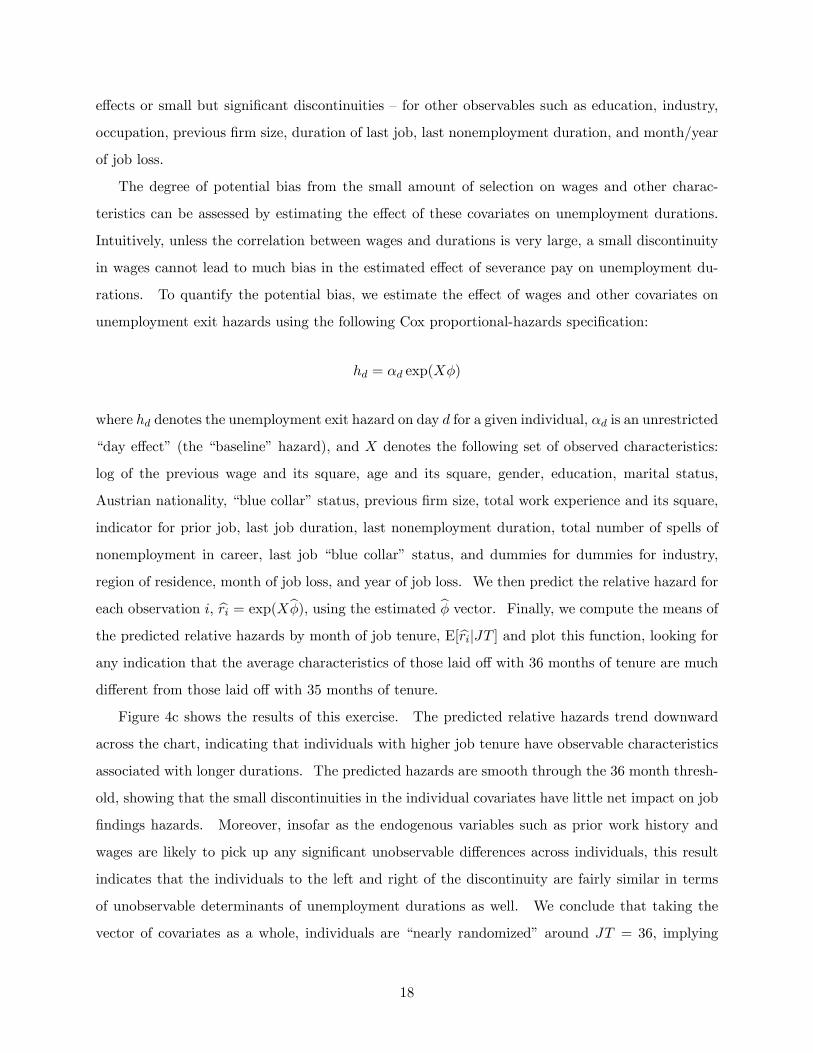
The degree of potential bias from the small amount of selection on wages and other charac-

teristics can be assessed by estimating the e¤ect of these covariates on unemployment durations.

Intuitively, unless the correlation between wages and durations is very large, a small discontinuity

in wages cannot lead to much bias in the estimated e¤ect of severance pay on unemployment du-

rations. To quantify the potential bias, we estimate the e¤ect of wages and other covariates on

unemployment exit hazards using the following Cox proportional-hazards speci�cation:

hd = �d exp(X�)

where hd denotes the unemployment exit hazard on day d for a given individual, �d is an unrestricted

�day e¤ect� (the �baseline�hazard), and X denotes the following set of observed characteristics:

log of the previous wage and its square, age and its square, gender, education, marital status,

Austrian nationality, �blue collar�status, previous �rm size, total work experience and its square,

indicator for prior job, last job duration, last nonemployment duration, total number of spells of

nonemployment in career, last job �blue collar� status, and dummies for dummies for industry,

region of residence, month of job loss, and year of job loss. We then predict the relative hazard for

each observation i, bri = exp(Xb�), using the estimated b� vector. Finally, we compute the means ofthe predicted relative hazards by month of job tenure, E[brijJT ] and plot this function, looking forany indication that the average characteristics of those laid o¤ with 36 months of tenure are much

di¤erent from those laid o¤ with 35 months of tenure.

Figure 4c shows the results of this exercise. The predicted relative hazards trend downward

across the chart, indicating that individuals with higher job tenure have observable characteristics

associated with longer durations. The predicted hazards are smooth through the 36 month thresh-

old, showing that the small discontinuities in the individual covariates have little net impact on job

�ndings hazards. Moreover, insofar as the endogenous variables such as prior work history and

wages are likely to pick up any signi�cant unobservable di¤erences across individuals, this result

indicates that the individuals to the left and right of the discontinuity are fairly similar in terms

of unobservable determinants of unemployment durations as well. We conclude that taking the

vector of covariates as a whole, individuals are �nearly randomized� around JT = 36, implying

18

that any signi�cant discontinuity in durations at this point can be attributed to severance pay.

Our identi�cation strategy for estimating the e¤ect of the UI bene�t extension on durations

is conceptually similar to the strategy for severance pay. Formally, we replace the indicator for

severance pay in equation (11) with an indicator E for extended bene�t status, and replace job

tenure with a measure of months worked (MW ) in the �ve years before the job termination.

Again, the potential problem with a simple regression of unemployment duration on EB status is

that people with a longer work history may be more (or less) likely to �nd a job quickly. And, as

in equation (10), the key assumption that facilitates an RD approach is that the expected value of

unobserved characteristics is the same for people with MW just under 36 months and just over 36

months. We evaluate this assumption by plotting the frequency of layo¤s, the average values of

various observable covariates, and the predicted unemployment exit hazards against MW . In the

interest of space, we do not report these results here. We �nd that there are no discontinuities

in the relative number of layo¤s, nor in the predicted relative hazard at MW = 36. Moreover, in

contrast to the situation in Figure 4b, there is no signi�cant jump in mean wages nor the other

covariates around the 36 month threshold in months worked. Overall, we conclude that the patterns

in the data are consistent with the assumption that EB status is �as good as randomly assigned�

among people with values of MW on either side of the 36 month threshold.

Identi�cation with Double Discontinuity. As noted above, although severance pay and EB status

depend on di¤erent running variables, there is a group of people in our sample �those with only

1 employer in the past 5 years �who reach the 36 month eligibility thresholds for severance pay

and EB�s at the same point. There are two ways to handle the resulting �double discontinuity�

problem. The �rst is to analyze a subsample in which the two discontinuities are not overlapping.

To implement this approach, we consider the �restricted sample�of individuals who worked for one

month or more within the past �ve years at a �rm di¤erent from the one from which they were

just laid o¤. Everyone is the restricted sample who has JT � 35 months has MW � 36 and thus

quali�es for EB. Thus, only severance pay eligibility shifts at JT = 36 in the restricted sample

(the fraction eligible for EB remains constant at 100% around JT = 36). Conversely, as months

worked approaches 36 months, no one in the subsample has yet worked 36 months at the same

employer. Thus, only EB status shifts at MW = 36 in the restricted sample. The separation of

the two discontinuities permits the use of conventional single-variable RD methods to identify the

severance and EB e¤ects in the restricted sample.

An alternative approach to separating the two e¤ects, which can be applied in the full sample, is

19

to explicitly model the joint e¤ects of severance pay and extended bene�ts. Consider the extended

model

y = �+ S�s + E�e + " (12)

where S and E are indicators for severance pay and EB eligibility, respectively.14 As in the

single discontinuity case, the problem for inference based on this model is that the unobserved

determinants of unemployment duration may be correlated with JT and/or MW . De�ne the

control function g(JT;MW ) as

E["jJT;MW ] = g(JT;MW ):

The key assumption needed is that g(JT;MW ) is continuous at JT = 36 for all values of MW ,

and continuous at MW = 36 for all values of JT . Under this identi�cation assumption, we can

augment equation (12) with the control function

y = �+ S�s + E�e + g(JT;MW ) + �

where � � " � E["jJT;MW ] is mean independent of E and S. Since S and E jump discontinu-

ously at JT = 36 and MW = 36, respectively, and JT and MW are imperfectly correlated, the

coe¢ cients �sand �e are identi�ed controlling for g. To implement this model, we assume as above

that g can be approximated by a low order polynomial of JT and MW .

VI E¤ects of Cash-In-Hand and Bene�t Extensions on Durations

This section presents the main results on the e¤ect of severance pay and UI bene�t extensions on

durations. We begin with a non-parametric graphical overview and then estimate a set of hazard

models to obtain numerical measures of the elasticities of interest.

VI.A Graphical Results

Severance Pay. We begin our analysis in Figure 5a by plotting mean nonemployment durations by

tenure-month category to give a preliminary sense of how the severance pay discontinuity a¤ects

search behavior. For simplicity, we ignore censoring (e¤ectively treating all measured durations as14Note that (12) does not include an interaction e¤ect between S and EB. While in principle we would like to

allow for an interaction between the two policies, in practice everyone with S = 1 has EB = 1. Hence the interactioncannot be identi�ed.

20

complete), and exclude all observations with a nonemployment duration of more than two years to

eliminate the long right tail of the distribution. Figure 5a shows that there is a clearly discernible

jump in the average nonemployment duration of approximately 10 days around the severance pay

discontinuity.

We cannot attribute the entire gap in Figure 5a to the e¤ect of the severance payment because

of the double discontinuity problem �the fraction of individuals receiving EB also jumps (by 20

percentage points) at the cuto¤. Given that the change in the EB policy applies to a small group

of individuals, one would expect that most of the discontinuity in durations at 36 months of job

tenure is due to severance pay. To isolate the pure e¤ect of severance pay using simple graphical

methods, we focus on the �restricted subsample�where the two discontinuities are not overlapping.

In particular, as described above, we consider the subset of individuals who have worked for at

least one month at another �rm within the past �ve years before joining the �rm from which they

were laid o¤. The restricted sample includes 83% of the observations in the full sample. Since

eligibility for EB is determined by total months worked within the past �ve years, the fraction of

individuals receiving EB in the restricted sample converges smoothly to 100% before the 36 month

job tenure cuto¤. Figure 5b replicates Figure 5a for this subsample. This �gure shows a jump

in the mean nonemployment duration of approximately 8 days at the 36 month cuto¤, con�rming

that most of the 10 day gap in Figure 5a is indeed caused by the severance payment.

A more precise approach to examining the e¤ect of severance payments on search behavior is

to examine how job �nding hazard rates change around the discontinuity. Figure 6 presents such

an analysis. In this �gure, we include all nonemployment durations and adjust the hazards for

censoring. We focus on the hazard rates over the �rst 20 weeks �the period of interest from the

perspective of testing between models since it includes only the time until the bene�t extension �by

censoring all observations at 140 days. To examine how average hazard rates vary across tenure-

month categories, we �t a Cox proportional-hazards model with dummies for the tenure-month

groups. We estimate the model in the full sample while adjusting for the double discontinuity

problem due to the EB e¤ect by including cubic polynomials in months worked and a dummy for

21

EB eligibility:

hd = �d expf�13I(j = 13) + �14I(j = 14) + :::+ �34I(j = 34) (13)

+ �36I(j = 36) + :::+ �58I(j = 58)

+ X + �EB + �1MW + �2MW 2 + �3MW 3

+ �E1 EB �MW + �E2 EB �MW 2 + �E3 EB �MW 3g

In this speci�cation, �d denotes the baseline hazard on day d of the spell, EB denotes an

indicator variable for extended-bene�ts eligibility,MW denotes the total number of months worked

in the past �ve years, and X denotes a set of covariates. The key coe¢ cients of interest are the

�js, which can be interpreted as percentage di¤erence between average hazard in group j and the

average hazard in j = 35 (the omitted group). Note that this method of estimating the �js

assumes a proportional shift in the hazard rates across the tenure-month categories. We have

also implemented a less parametric approach of stratifying the baseline hazards by tenure-month

category (permitting �jd to vary freely across tenure-month categories j), and then examining how

the average estimated �jd varies with j. This approach yields very similar results to the ones

reported below.

Figure 6a plots the estimated �js without any additional controls (no X). Consistent with the

results in Figure 5, this �gure shows that there is a discontinuous drop of approximately 10% in

the hazard rate at the severance pay discontinuity. Since the estimated relative hazards in this

�gure are adjusted for the EB e¤ect, the entire jump in this �gure can be attributed to the e¤ect

of severance pay in the full sample.

As noted by Lee and Card (2006), one of the appealing features of a regression discontinuity

approach is that estimates of the discontinuity should be invariant to the presence or absence

of control variables.15 As in a classical experimental design, however, the addition of controls

may lead to some gain in precision. Moreover, a comparison of the estimated discontinuities

with and without controls provides an informal speci�cation test that the underlying smoothness

assumptions required for an RD approach are valid. Figure 6b replicates Figure 6a adjusting for

a set of observable covariates by including the following set of controls in the X vector: female,

�blue collar� status, marital status, Austrian nationality, age and its square, log wage and its

15Note that in our presentation of the RD method we exclude controls. One can think of the " term as includingthe e¤ect of all the characteristics that vary across the sample, including potentially observable as well as unobservedcharacteristics.

22

square, dummies for month and year of job loss. As in Figure 6a, the job �nding hazard shows

about a 10% drop at the 36 month threshold for receiving severance pay. The similarity of the

discontinuities in the estimated hazards with and without other controls is consistent with the

result in Figure 4c that the relationship between the hazards and observable covariates is smooth,

and validates the assumptions of the RD approach.

A potential concern in Figures 6a and 6b is that there is some seasonality in the hazard rates

associated with job tenure. In particular, the hazard rates in the last few months of each tenure-year

(e.g. months 21-23, 33-35, etc.) are approximately 2.5% higher than the hazards in the remainder

of the tenure-year. One explanation for this pattern is that individuals who leave a �rm shortly

after completion of a full year of service are di¤erent from those who leave just before completion

of a full year. Such di¤erences may arise e.g. because of vesting rules for pension plans that take

e¤ect at integer thresholds or because planned terminations are more likely to take place after a

full year of service is complete. Since the severance pay cuto¤ falls at an integer threshold (three

years of tenure), one may be concerned that the seasonality in hazards biases the RD estimate of

the severance pay e¤ect. To gauge the size of the potential bias, we adjust for tenure seasonality

by estimating a parametric RD model with an �end of tenure year� indicator which equals 1 in

the three months before the end of each tenure year (21-23, 33-35, 45-47, and 57-59). We then

adjust the average hazards in Figure 6a for seasonality by subtracting the estimated end of tenure

year e¤ect from the hazard rates at the end of each tenure year.16 Figure 6c plots the resulting

seasonality-adjusted hazards. This �gure shows that the seasonality adjustment fully eliminates

the potentially worrisome patterns in Figures 6a and 6b. With this adjustment, the average hazard

rate falls by approximately 8% at the severance pay cuto¤, indicating that the results are essentially

robust to the seasonality concern.

As noted above, the causal interpretation of our results relies on the identi�cation assumption

that there would be no systematic di¤erences in nonemployment durations between individuals laid

o¤ just after three years of tenure and those laid o¤ just before three years absent the discontinuous

severance pay treatment. The rich panel structure of our dataset allows a simple �placebo�test to

further evaluate the validity of this assumption. In Figure 7, we examine how job tenure at the job

before the one just lost �which is smoothly related to severance pay eligibility for the current layo¤

�is related to the current duration of nonemployment. We restrict attention to the individuals who

16More precisely, we estimate speci�cation (3) in Table 3 with the end of tenure dummy and subtract the coe¢ cientestimate from hazard rates at the end of each tenure year in Figure 6a.

23

have job tenure of between 1 and 5 years at a job prior to the one they just lost. This �gure shows

that mean nonemployment durations evolve smoothly through the 36 month cuto¤, supporting our

identi�cation assumption. This result indicates that any alternative omitted-variable explanation

of our �ndings would require that individual�s unobserved characteristics change over time such

that a discontinuity in nonemployment durations at 36 months emerges only in the current job.

Thus far we have summarized the e¤ect of severance pay on search behavior in a single statistic,

either mean durations or the average job �nding hazard over the �rst twenty weeks of the spell. We

now explore how severance pay a¤ects search behavior as the spell elapses. Figure 8a plots average

weekly job �nding hazards for individuals laid o¤ in tenure-months 33-35 (no severance) and those

laid o¤ in months 36-38 (who receive severance). The �gure shows that the gap between the

hazard rates in the two groups emerges after week 5 of the spell, and gradually narrows starting

around week 25. This delayed, temporary e¤ect of severance pay on search behavior may be

consistent with a bu¤er stock model where agents become increasingly liquidity constrained as the

spell elapses, making cash grants more relevant later in the spell.

We interpret Figures 5-8 as showing that the provision of cash-in-hand through a lump sum

severance payment substantially lowers job �nding rates. This evidence rejects the full insurance

(PIH with complete markets) model based on prediction 1 in Table 1.

Extended Bene�ts. We now replicate the preceding analysis for the extended bene�t policy.

Figure 9a plots the relationship between average nonemployment durations and months worked

(MW ) in the past �ve years in the full sample. As in Figure 5a, we ignore censoring and exclude

observations with a nonemployment duration of more than 2 years. Figure 9a shows that there is

a clearly discernible jump in the average nonemployment duration of approximately 7 days around

the EB discontinuity. Figure 9b replicates Figure 9a in the restricted sample, where the entire

discontinuity at MW = 36 can be attributed to EB. This �gure con�rms that the discontinuity

in EB eligibility is in fact responsible for the jump in nonemployment durations in Figure 9a, since

the fraction receiving severance pay evolves smoothly through MW = 36 in this subsample.

In Figure 9c, we examine how the average hazard rates over the �rst twenty weeks of the spell

vary around the EB discontinuity. We estimate a proportional hazard model analogous to that in

(13), with group dummies for months worked instead of job tenure. We include a cubic polynomial

in job tenure and a dummy for severance pay eligibility to identify the pure e¤ect of the EB policy

on hazard rates in the full sample. Consistent with the results in Figures 9a-b, this �gure shows

that there is a discontinuous drop of approximately 7% in the average hazard rate prior to week at

24

the EB discontinuity.

In Figure 8b, we explore how extending UI bene�ts a¤ects search behavior as the spell elapses,

comparing the weekly job �nding hazards for individuals in the three months to the left and right

of the MW = 36 discontinuity. This �gure shows that the bene�t extension has a large e¤ect on

behavior after week 20, but also has a substantial e¤ect on search behavior prior to week 20, i.e.

before the agent actually receives any additional income. This provides clear evidence that at least

some individuals are forward-looking, in that they take into account their future expected income

stream when searching in the early weeks of the spell. This �nding rejects the complete myopia

(rule of thumb) model based on prediction 2 in Table 1.

In the next section, we estimate the severance pay and EB e¤ects using parametric hazard

models, and con�rm the visual evidence.

VI.B Hazard Model Estimates

To more precisely quantify the e¤ects of severance pay and extended bene�ts on the duration of

job search we estimate a series of proportional hazards models for the risks of �nding a new job

or exiting unemployment. These models include unrestricted daily baseline hazards, indicators

for eligibility for severance pay and extended bene�ts (S and E, respectively), and third-order

polynomials in job tenure (JT ) and and months of work in the previous 5 years (MW ) that allow

the derivative of the control function to change discontinuously at the eligibility cuto¤s:

hd = �d expf�sS + �eEB + X+ (14)

+ �1JT + �2JT + �3JT3

+ �S1S � JT + �S2S � JT 2 + �S3S � JT 3

+ �1MW + �2MW 2 + �3MW 3

+ �E1 EB �MW + �E2 EB �MW 2 + �E3 EB �MW 3g

In all cases we censor the spells at 139 days in order to isolate the e¤ects of the policy variables

in the �rst 20 weeks of job search, prior to the point at which extended bene�ts become available.

Thus, the estimated e¤ect of extended bene�ts can be interpreted as the e¤ect of future bene�ts

on current search activity.

Tables 3a and 3b present the estimated coe¢ cients �s and �e from a set of alternative samples

25

and speci�cations. We begin in columns 1 and 2 by estimating the e¤ects of the severance pay

and EB policies separately in the restricted sample without any controls. The coe¢ cient estimates

indicate that both severance pay and EB reduce job �nding hazards substantially, consistent with

the visual evidence documented above. In column 3, we estimate the two e¤ects jointly in the full

sample using the �double RD� control function approach in (14). These estimates corroborate

that the results in the full sample are similar to those in the restricted sample.

We evaluate the robustness of these results by including additional covariates in the double RD

speci�cation with the full sample in speci�cations 4 and 5. In speci�cation 4, we control for the

worker�s gender, marital status, Austrian nationality, �blue collar�occupation indicator, age and

its square, log previous wage and its square, as well as dummies for the month and year of the job

termination. In speci�cation 5, we add to this set of controls the �end of tenure year� dummy

de�ned above to correct for tenure seasonality. The estimates indicate the results are robust to

these changes in the covariate set.

Table 3b presents additional robustness checks and placebo tests. In speci�cation 6, we expand

the set of covariates in speci�cation 4 of Table 3a to include the following additional covariates that

capture the individual�s work history: education, total number of employees at �rm from which the

work was laid o¤, total years of work experience and its square, �blue collar� status at job prior

to the one lost, indicator for having a job before the one just lost, total number of nonemployment

spells in the career, a dummy for being recalled to the job before the one just lost, the duration

of the job before the one just lost, the last nonemployment duration before the current spell, and

dummies for prior industry and region of residence. The inclusion of this rich set of endogenous

covariates does not change the estimates, which perhaps helps mitigate concerns about bias due to

selection.

In speci�cation 7, we take an alternative approach to dealing with the tenure seasonality problem

described above by excluding all observations in the last three months of each tenure year (tenure

months 21-23, 33-35, etc.) and replicating speci�cation 3 of Table 3a. In speci�cation 8, we

examine the robustness of our results to measuring durations by time registered as unemployed

instead of time between jobs. We code observations where the end of registered unemployment

does not coincide with the start of a new job as censored and replicate speci�cation 3 of Table 3b

with this alternative duration measure. The estimates indicate that the results are robust to these

speci�cation checks.

The last three columns of Table 3b report estimates of the �placebo test� corresponding to

26

Figure 7 by examining how tenure at the previous job and months worked prior to the relevant

period for EB eligibility a¤ects job �nding hazards. To obtain a sample consistent with the one

we use for our main analysis, we restrict attention to the individuals who (a) have job tenure of

between 1 and 5 years at a job prior to the one they just lost and (b) worked for between 1 and 5

years of the �ve years preceding the last �ve years (i.e., years -10 to -5 before the current job loss

date). We then estimate the e¤ect of the severance pay and EB placebos �de�ned as having more

than 36 months of job tenure at the job before the one just lost and having more than 36 months

of work experience between years -10 and -5, respectively. Speci�cation 9 reports these estimates

for a model analogous to speci�cation 3 without any controls, while speci�cation 10 replicates 9

with the control set used in speci�cation 4. Both sets of estimates con�rm that there is no placebo

e¤ect, consistent with Figure 7. Finally, in speci�cation 11, we also include the true severance

pay and EB eligibility indicators, along with the placebo indicators and cubic polynomials for all

four running variables. The true severance pay and EB variables still are estimated to reduce job

�nding hazards substantially (though the standard errors rise because the sample is one-�fth the

original size). The hypothesis that the placebo and true severance pay e¤ects is rejected with

p = 0:06.

We have �t a wide variety of other speci�cations in an e¤ort to probe the robustness of the

results in Table 3. We �nd that estimates from alternative models �especially the ratio of the

severance pay and EB e¤ect �are quite stable. For example, replacing the third-order polynomials

with fourth order models leads to estimated severance pay and EB e¤ects that are a little bigger

in magnitude than those reported in Table 3. Trimming outliers, dropping those recalled at the

job prior to the one just lost, and estimating the e¤ects of the two policies on average hazards over

the �rst six months or year of the spell also yields similar results.

VII Search Outcomes

Having found that severance pay and extended bene�ts increase the duration of job search, it is

interesting to ask whether this increased duration leads to any di¤erences in the nature of the jobs

obtained through the search process. Models with a non-degenerate distribution of potential job

qualities predict that job searchers with more assets and longer bene�ts will raise their reservation

job quality threshold, leading to a rise in the average quality of accepted jobs. As above, we begin

with a graphical overview of the main �ndings and then present regression estimates.

27

VII.A Graphical Results

The �rst measure of job quality we examine is the wage on the next job. De�ne gi = log(wni ) �

log(wpi ) where wni is individual i

0s wage in the �rst year at the next job and wpi is his wage in the

�nal year at the previous job. Note that gi is missing for 15% of the sample, most of which is

accounted for by individuals who do not �nd a new job before the end of the sampling period.

Figure 10a plots the average value of gi, excluding outliers where jgij > 2 (which account for 0.65%

of observations with non-missing gi), in each tenure-month cell. The smoothness of wage growth

rates through the 36 month discontinuity indicates that the increased duration of search induced

by severance payments does not yield any improvements in ex-post wages.

Even if there are no bene�ts in terms of wages, it is possible that individuals could jobs with

higher quality in other dimensions. One convenient summary statistic for the quality of subsequent

jobs is their duration (e.g., Jovanovic 1979). Figure 10b shows the relationship between job tenure

on the previous job and the average hazard of leaving the next job over the �rst two years at the

job. We calculate the average job leaving hazard by �rst computing the monthly hazard rates of

exiting the next job within each tenure-month category. We then take an unweighted average of

these monthly hazards over the �rst two years at the next job to arrive at the values plotted in the

�gure. The job-leaving hazards are smooth through the discontinuity, indicating that workers who

received severance pay do not stay at their next jobs any longer than those who did not receive

severance pay.

We replicate the same analysis for the EB policy in Figure 11 by changing the running variable

on the x-axis to months worked in the past �ve years. Again, we �nd that both wages and

subsequent job-leaving hazards are smooth through the EB discontinuity, indicating that there is

no evidence of match quality gains from extending durations through provision of extended bene�ts

either.

We also checked for match e¤ects by replicating Figures 10 and 11 for several other measures:

the probability of moving across regions of Austria, the probability of switching industries, the

probability of switching from a �blue collar� to a �white collar� occupation, the mean log wage

in the �ve years following the unemployment spell, and the size of the next �rm. In addition,

we examined percentiles of the wage distribution to check if there are gains in the tails of the

distribution. We found no discontinuity in any of these measures for either the EB or severance

pay policy. We also split the data into subgroups (e.g. by age, gender, wage, education) and found

28

no evidence of match e¤ects in any of the subgroups.

VII.B Regression Estimates

To provide a more formal summary of the job quality e¤ects associated with severance pay and

extended bene�ts, we modelled the impacts of these variables on the change in log wages (from the

old job to the new job) and on the hazard rate of leaving the new job within the �rst two years,

using double RD speci�cations similar to the ones in Table 3.

Table 4 reports the results of this analysis. Speci�cation 1 examines the e¤ect of severance

pay and EB on wage growth without any controls. Speci�cation 2 add the full set of observables

described above to this regression. Speci�cation 3 reports coe¢ cient estimates from a hazard model

for the duration of the new job without controls, while speci�cation 4 replicates this estimation

with controls. The results of the analysis are consistent with the �gures: there is no evidence on

match quality gains in any of the speci�cations.

An important distinction between the present analysis of job quality e¤ects and some earlier

studies that have failed to detect evidence of quality gains is the precision of the estimates. The

regression estimates and �gures show that even a small improvement in wages or subsequent job

tenure (e.g. 1%) would be detectable in our analysis. Hence, our evidence suggests that the job

quality gains from extending unemployment durations are not merely statistically insigni�cant, but

small in magnitude.

One caveat is that the Austrian labor market is characterized by nearly 100% coverage under

collective bargaining agreements. Relative to other less regulated labor markets, the range of vari-

ation in the quality of jobs available to a given worker may be somewhat compressed. Nevertheless,

as noted in section IV, the variation in wage changes experienced by job losers is relatively wide

(�(� logw) = 0:51) and is comparable to variability measured among displaced workers in the U.S.

VIII Calibration: Location on the Continuum

In this section we use the model outlined in Section III to interpret our main empirical �ndings.

For convenience we restate the key prediction (equation (9)) giving the relative e¤ects of severance

pay and extended bene�ts on the optimal choice of search intensity (s�t ;the probability of �nding a

job):@s�t =@At@s�t =@bt+1

= D � 1 + r

1� s�t+1

29

where

D =u0(cut )� u0(cet )

u0(cut+1):

Note that the coe¢ cient �s from our RD model gives the e¤ect of a severance payment equal to 2

months of salary (exempt from most taxes) on the exit hazard in the �rst 140 days of job search.

Since we use a proportional hazards speci�cation, �s � @ log s�t =@At�2w(1�:06)=(1��), where w is

the net (after-tax) monthly wage, � is the average tax rate on earned income (approximately 30%),

and 6% is the approximate tax rate that applies on severance payments. 17 Likewise, the coe¢ cient

�e from our RD models gives the e¤ect of eligibility for 10 additional weeks (or 2.5 months) of

regular UI bene�ts. The net income from extended bene�ts is approximately 2:5w�(1� UA=UI),

where � is the replacement rate of regular UI bene�ts (relative to net salary w), and UA=UI

represents the ratio of unemployment assistance (UA) bene�ts to UI bene�ts for a typical worker

who would exhaust regular UI after 20 weeks in the absence of the bene�t extension. The statutory

replacement rate for UI bene�ts is 55%. However, most workers receive supplementary UI bene�ts

for their children: on average we estimate that this raises the replacement rate to 64%. 18 O¤setting

this is the fact that workers in Austria receive 14 �monthly�salaries per year �12 monthly salaries

plus 2 bonus months �whereas UI bene�ts are monthly. Thus the average e¤ective replacement rate

is � = 0:64� 12=14 = 0:55. Bene�ts for UA are based on a formula: UA = 0:92UI �F +A, where

F represents other family member�s earnings and A represents dependent allowances (currently 423

Euros per month for a partner and 213 Euros per month for each dependent child). Data from the

2004 Survey of Income and Living Conditions show that the average wage earner between the ages

of 20 and 49 in Austria contributes just under one-half of his/her family income. This suggests

that in our sample F is approximately equal to w. Assuming a typical job loser has a partner and

2 children, and that the ratio of family allowances to average net monthly income is constant, we

estimate that UA=UI = 0:38. Combining these pieces, the coe¢ cient �e from our RD models

provides an estimate of @ log s�t =@bt+1 � 2:5w � 0:55 � (1 � 0:38):19 The predicted value for the

17The fraction of people who �nd a job in under N days is approximately the product of the daily hazard ratesup to day N (assuming the daily hazard is small). Thus, the e¤ect of some variable on the log of the probability of�nding a job within N days is approximately equal to the e¤ect on the log hazard rate.18Unfortunately, our data source does not contain information on the dependent allowances available to an unem-

ployed worker. We used a variety of sources to compare actual average UI bene�ts to average net salaries.191.2w = 2.5 months � 55% replacement rate � 87% change of not getting UA bene�ts.

30

ratio of the coe¢ cients �sand �e is therefore:

�s�e

=@s�t =@At@s�t =@bt+1

� 2w(1� :06)=(1� 0:3)2:5w � 0:55� (1� 0:38) = 3:15�

@s�t =@At@s�t =@bt+1

= 3:15�D � 1 + r

1� s�t+1:

Given a value of D;we need to multiply by 3:15(1+r) and divide by (1�s�t+1) to obtain a prediction

for �s=�e . The latter term adjusts future unemployment bene�ts for the probability they will be

received. Interpreting period t as the �rst 20 weeks of job search, this adjustment factor is just

the probability of not �nding a job within 20 weeks, which is approximately 35 percent. Treating

r as small (as it only applies over a 20 week period) gives:

�s�e= 9D.

Two Benchmarks. As we noted in Section III, our theoretical model is su¢ ciently general to nest a

wide range of preferences and �nancial environments faced by job seekers. Di¤erent degrees of risk

aversion and di¤erent abilities to borrow and lend over the course of a spell of unemployment will

predict di¤erent values for the ratio D, and lead to di¤erent predictions for the relative magnitude

of the severance pay and EB e¤ects in our models. Here we consider two cases that represent useful

bounds: the case where individuals have unrestricted access to credit at a �xed interest rate �the

permanent income hypothesis (PIH) benchmark; and the case where individuals set consumption

equal to income in each period �the credit constrained benchmark.20

Assume that the family income of a job seeker includes his or her earnings or UI bene�ts,

and other sources that total F (euros per month). Let � = w=(w + F ) denote the share of the

job-seeker�s earnings in total family income. In the cash-constrained case, cet = w + F , and

cut = bt + F = �tw+ F , where �t is the replacement rate in period t. Assuming that u(c) is in the

constant relative risk aversion class,

D =u0(bt + F )� u0(w + F )

u0(bt+1 + F )

=u0((��t + (1� �))� u0(1)u0((��t+1 + (1� �))

20Given the evidence that unemployment responds to severance pay, we rule out the "full insurance" case. Likewise,given that eligibility for EB�s a¤ects the exit rate from unemployment in the �rst 20 weeks of unemployment, we ruleout the "fully myopic" case.

31

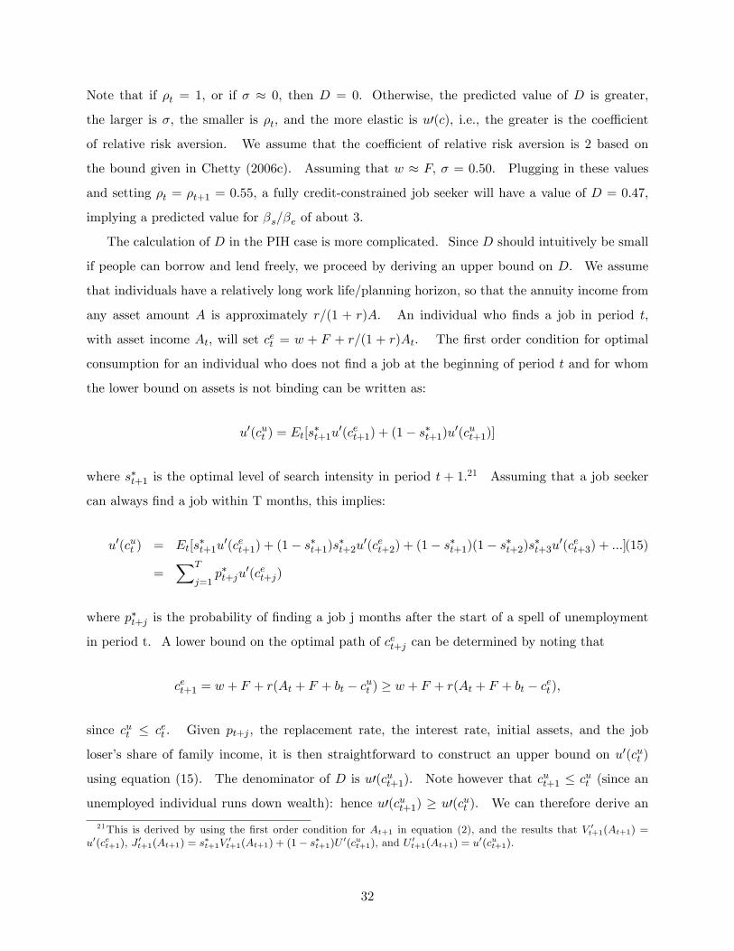
Note that if �t = 1, or if � � 0, then D = 0. Otherwise, the predicted value of D is greater,

the larger is �, the smaller is �t, and the more elastic is u0(c), i.e., the greater is the coe¢ cient

of relative risk aversion. We assume that the coe¢ cient of relative risk aversion is 2 based on

the bound given in Chetty (2006c). Assuming that w � F; � = 0:50. Plugging in these values

and setting �t = �t+1 = 0:55, a fully credit-constrained job seeker will have a value of D = 0:47,

implying a predicted value for �s=�e of about 3.

The calculation of D in the PIH case is more complicated. Since D should intuitively be small

if people can borrow and lend freely, we proceed by deriving an upper bound on D. We assume

that individuals have a relatively long work life/planning horizon, so that the annuity income from

any asset amount A is approximately r=(1 + r)A. An individual who �nds a job in period t,

with asset income At, will set cet = w + F + r=(1 + r)At. The �rst order condition for optimal

consumption for an individual who does not �nd a job at the beginning of period t and for whom

the lower bound on assets is not binding can be written as:

u0(cut ) = Et[s�t+1u

0(cet+1) + (1� s�t+1)u0(cut+1)]

where s�t+1 is the optimal level of search intensity in period t + 1.21 Assuming that a job seeker

can always �nd a job within T months, this implies:

u0(cut ) = Et[s�t+1u

0(cet+1) + (1� s�t+1)s�t+2u0(cet+2) + (1� s�t+1)(1� s�t+2)s�t+3u0(cet+3) + :::](15)

=XT

j=1p�t+ju

0(cet+j)

where p�t+j is the probability of �nding a job j months after the start of a spell of unemployment

in period t. A lower bound on the optimal path of cet+j can be determined by noting that

cet+1 = w + F + r(At + F + bt � cut ) � w + F + r(At + F + bt � cet );

since cut � cet . Given pt+j , the replacement rate, the interest rate, initial assets, and the job

loser�s share of family income, it is then straightforward to construct an upper bound on u0(cut )

using equation (15). The denominator of D is u0(cut+1). Note however that cut+1 � cut (since an

unemployed individual runs down wealth): hence u0(cut+1) � u0(cut ). We can therefore derive an

21This is derived by using the �rst order condition for At+1 in equation (2), and the results that V 0t+1(At+1) =

u0(cet+1), J0t+1(At+1) = s

�t+1V

0t+1(At+1) + (1� s�t+1)U 0(cut+1), and U 0t+1(At+1) = u0(cut+1):

32

upper bound on D by constructing an upper bound for D� = (u0(cut )� u0(cet ))=u0(cut ) � D.

As we noted in the discussion of Table 2, most of the people in our sample of job losers who are

observed returning to work within 5 years have returned by 18 months. The re-employment hazard

rate after 18 months is extremely low (less than 1% per month), suggesting that many of those

who are not back to work within 18 months have taken either a temporary break (e.g., a maternity

leave) or have found a job outside the country or in the public sector or in self-employment. For

purposes of calibrating the PIH benchmark, we set T=18, and use the observed distribution of

waiting times to a new job in our sample to estimate p�t+j .22 We calculate the distribution of

times to re-employment ignoring those who are censored after 18 months.23

The term in the numerator ofD (orD�) re�ects the reaction of job losers to the increase in assets

when they receive severance pay. Since everyone who is eligible for severance pay receives EB�s,

we assume that �t = 0:55, for the �rst 30 weeks of unemployment, and that �t = 0:55 � UA=UI

thereafter, using the same calculations as above to set UA=UI = 0:38. We also assume that a

typical job loser contributes 50% of his or her family income, and that at the time of job loss assets

are 0. Assuming that the coe¢ cient of relative risk aversion is 2, and that individuals face an

annual interest rate of 5%, we obtain the prediction D� = 0:010. Raising the interest rate to 10%

leads to a predicted value D� = 0:028.24 Taking 5% as a reference, the PIH benchmark suggests

that the ratio of the severance pay e¤ect to the EB e¤ect should be roughly 0.1.

Comparing the Empirical Estimate to the Benchmarks. How do our estimates of the relative

e¤ects of severance pay and extended bene�ts compare to these benchmarks? For purposes of

this exercise, we focus initially on the double discontinuity speci�cation in column 1 of Table 3b,

which includes a broad set of controls. This model yields an estimate of �s = �0:094 (standard

error=0.019) and an estimate of �e = �0:064 (standard error=0.018). Thus our estimated ratio

is �s=�e = 1:47, with a standard error of 0.30.25 This estimate is roughly halfway between

the prediction from the simple PIH model and the prediction from the credit-constrained model.

Moreover, the estimate is precise enough to rule out a value below 0.8 or above 2.1 at conventional

signi�cance levels.

22Note that as written our model implies that search intensity (which is also the probability or returning to work)rises over the spell of unemployment, since assets are decreasing (see also Lenz and Tranaes, 2004). More realistically,the marginal cost of search will rise over time as people exhaust their best leads for �nding a new job.23The resulting distribution has a 17% probability of re-employment within a month, 45% within 3 months, 71%

within 6 months, and 93% within a year.24Reducing the coe¢ cient of relative risk aversion to 1.5, we get the prediction D� = 0:008 if r=5% and D� = 0:017

if r=10%.25We calculated the standard error using the delta method. The estimates of �eand �e are slightly negatively

correlated.

33

One useful thought experiment is to ask: what interest rate would we have to assume in the

PIH model to generate a predicted value for the ratio �s=�e at the lower bound of the con�dence

interval? The answer is a 42% annual interest rate. Even with a 33% interest rate � the rate

suggested by Carroll (2001) to capture precautionary savings motives given his preferred income

generating model � the predicted value of �s=�e is only 0.45. Thus, we interpret the relative

magnitude of the estimates of �s and �e in Table 3 as providing fairly strong evidence against the

PIH benchmark.

IX Conclusion

In this paper, we used discontinuities in the Austrian unemployment bene�t system to distinguish

between commonly used models of dynamic household behavior. We reached three main �ndings:

(1) A cash grant equivalent to two months of wages induces substantial changes in search behavior

beyond what would be predicted by a benchmark lifecycle model without liquidity constraints;

(2) extending UI bene�ts also a¤ects search behavior early in the spell, providing evidence that

households are somewhat forward-looking; and (3) lengthening durations through EB and severance

pay policies has little or no e¤ect on subsequent job match quality. Using a model that nests a

continuum of cases from perfect smoothing to complete myopia, we conclude that the evidence favors

a model of job search with varying job search intensity and incomplete consumption smoothing.

We also provide a metric based on the ratio of the severance pay and EB e¤ects that can be used

to calibrate dynamic models of household behavior to our empirical �ndings.

These results have several implications for macroeconomics and public �nance. At a broad

level, they suggest that temporary changes in income have more important economic consequences

than traditional models suggest. For example, households�sensitivity to cash-in-hand suggests that

temporary �scal policy changes such as tax cuts could have signi�cant e¤ects on the economy. The

evidence of imperfect smoothing also suggests that there may be a signi�cant role for temporary

income assistance programs such as unemployment insurance, temporary welfare, and workers

compensation. The �nding that cash grants change search behavior in a manner similar to UI

bene�t extensions also suggests that much of the behavioral response to temporary bene�t social

insurance programs is an �income�or liquidity e¤ect rather than moral hazard caused by distortion

in relative prices (Chetty 2006b). Analyzing these issues formally in dynamic models calibrated

to match the evidence documented here is an interesting direction for further research.

34

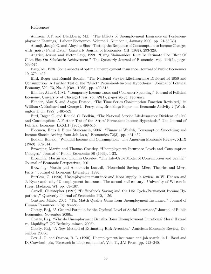
References

Addison, J.T. and Blackburn, M.L. �The E¤ects of Unemployment Insurance on Postunem-ployment Earnings,�Labour Economics, Volume 7, Number 1, January 2000, pp. 21-53(33)

Altonji, Joseph G. and Aloysius Siow �Testing the Response of Consumption to Income Changeswith (noisy) Panel Data,�Quarterly Journal of Economics, CII (1987), 293-328.

Angrist, Joshua and Victor Lavy, 1999. �Using Maimonides�Rule To Estimate The E¤ect OfClass Size On Scholastic Achievement,�The Quarterly Journal of Economics vol. 114(2), pages533-575.

Baily, M., 1978. Some aspects of optimal unemployment insurance. Journal of Public Economics10, 379�402.

Bird, Roger and Ronald Bodkin, �The National Service Life-Insurance Dividend of 1950 andConsumption: A Further Test of the �Strict�Permanent-Income Hypothesis.�Journal of PoliticalEconomy, Vol. 73, No. 5 (Oct., 1965), pp. 499-515

Blinder, Alan S, 1981. "Temporary Income Taxes and Consumer Spending," Journal of PoliticalEconomy, University of Chicago Press, vol. 89(1), pages 26-53, February.

Blinder, Alan S. and Angus Deaton, �The Time Series Consumption Function Revisited,� inWilliam C. Brainard and George L. Perry, eds., Brookings Papers on Economic Activity 2 (Wash-ington D.C., 1985) , 465-521

Bird, Roger C. and Ronald G. Bodkin, �The National Service Life-Insurance Divident of 1950and Consumption: A Further Test of the �Strict�Permanent-Income Hypothesis,�The Journal ofPolitical Economy, LXXIII (1965), 499-515.

Bloemen, Hans & Elena Stancanelli, 2005. �Financial Wealth, Consumption Smoothing andIncome Shocks Arising from Job Loss,�Economica 72(3), pp. 431-452.

Bodkin, Ronald, �Windfall Income and Consumption,�The American Economic Review, XLIX(1959), 602-614.

Browning, Martin and Thomas Crossley, �Unemployment Insurance Levels and ConsumptionChanges,�Journal of Public Economics 80 (1999), 1-23.

Browning, Martin and Thomas Crossley, �The Life-Cycle Model of Consumption and Saving,�Journal of Economic Perspectives, 2001.

Browning, Martin and Annamaria Lusardi, �Household Saving: Micro Theories and MicroFacts,�Journal of Economic Literature, 1996.

Burtless, G. (1990), Unemployment insurance and labor supply: a review, in W. Hansen andJ. Byearsand, eds, �Unemployment insurance: The second half-century�, University of WisconsinPress, Madison, WI, pp. 69�107.

Carroll, Christopher (1997) �Bu¤er-Stock Saving and the Life Cycle/Permanent Income Hy-pothesis,�Quarterly Journal of Economics 112, 1-56.

Centeno, Mário. 2004. �The Match Quality Gains from Unemployment Insurance.� Journal ofHuman Resources 39(3): 839-863.

Chetty, Raj, �A General Formula for the Optimal Level of Social Insurance,�Journal of PublicEconomics, November 2006a.

Chetty, Raj, �Why do Unemployment Bene�ts Raise Unemployment Durations? Moral Hazardvs. Liquidity,�UC-Berkeley mimeo, 2006b.

Chetty, Raj, �A New Method of Estimating Risk Aversion.�American Economic Review, De-cember 2006c.

Cox, J. C. and Oaxaca, R. L. (1990), Unemployment insurance and job search, in L. Bassi andD. Crawford, eds, �Research in labor economics�, Vol. 11, JAI Press, pp. 223�240.

35

Danforth, J. P. (1979): On the Role of Consumption and Decreasing Absolute Risk Aversionin the Theory of Job Search," in Studies in the Economics of Search, ed. by S. A. Lippman, andJ. J. McCall, pp. 109{31. North-Holland, New York.

Deaton, A. (1992), Understanding Consumption, Oxford University Press, Oxford.DiNardo, John and David Lee, �Economic Impacts of New Unionization on U.S. Private Sector

Employers: 1984-2001,�Quarterly Journal of Economics, 2004, 119(4), 1383-1442.Ehrenberg, R. and Oaxaca, R. (1976), �Unemployment insurance, duration of unemployment,

and subsequent wage gain�, American Economic Review 66(5), 754�766.Flavin, M. A. (1981), �The adjustment of consumption to changing expectations about future

income�, Journal of Political Economy 89(5), 974�1009.Flemming, J., 1978. Aspects of optimal unemployment insurance. Journal of Public Economics

10, 403�425.Gruber, Jonathan, �The Consumption Smoothing Bene�ts of Unemployment Insurance,�Amer-

ican Economic Review 87 (1997), 192-205.Hahn, Jinyong & Todd, Petra & Van der Klaauw, Wilbert, 2001. �Identi�cation and Estimation

of Treatment E¤ects with a Regression-Discontinuity Design,�Econometrica vol. 69(1), pages 201-09, January.

Hall, Robert and F.S. Mishkin �The Sensitivity of Consumption to Transitory Income: Esti-mates from panel data on households,�Econometrica, 1982.

Hansen, G. D., and A. Imrohoroglu (1992), �The Role of Unemployment Insurance in an Econ-omy with Liquidity Constraints and Moral Hazard,�Journal of Political Economy, 100(1), 118-42.

Hsieh, Chang-Tai, �Do Consumers Respond to Anticipated Income Shocks? Evidence from theAlaska Permanent Fund.�American Economic Review, March 2003.

Johnson, David & Jonathan A. Parker & Nicholas S. Souleles, 2004. �Household Expenditureand the Income Tax Rebates of 2001,�American Economic Review, 2006.

Jovanovic, Boyan (1979) Job matching and the theory of turnover. Journal of Political Economy87, pp. 972�990.

Katz, Lawrence and Bruce Meyer, The Impact of the Potential Duration of UnemploymentBene�ts on the Duration of Unemployment,�Journal of Public Economics 41 (1990) 45-72.

Lalive, Rafael, Jan C Van Ours, and Josef Zweimuller, �How Changes in Financial IncentivesA¤ect the Duration of Unemployment,�Review of Economic Studies, forthcoming.

Lee, David �Randomized Experiments from Non-random Selection in U.S. House Elections,�Journal of Econometrics, forthcoming, 2006.

Lee, David and David Card, �Regression Discontinuity Inference with Speci�cation Error,�National Bureau of Economic Research Technical Working Paper #322, 2006.

Lentz, Rasmus and and Torben Tranaes, �Job Search and Savings: Wealth E¤ects and DurationDependence,�Journal of Labor Economics, volume 23 (2005), pages 467�489.

Meyer, B., 1990. Unemployment insurance and unemployment spells. Econometrica 58 (4),757�782.

Parker, Jonathan, 1999. "The Reaction of Household Consumption to Predictable Changes inSocial Security Taxes," American Economic Review, American Economic Association, vol. 89(4),pages 959-973, September

Shimer, Robert and Ivan Werning, �Reservation Wages and Unemployment Insurance,�Univ.of Chicago mimeo, 2006.

Souleles, Nicholas (1999), �The Response of Household Consumption to Income Tax Refunds,�American Economic Review vol. 89(4), pages 947-958, September.

Thistlewaite, D. and D. Campbell, �Regression-Discontinuity Analysis: An Alternative to theEx Post Fact Experiment,�Journal of Educational Psychology, 51, 309�317.

36

Wang, Cheng & Williamson, Stephen, 1996. �Unemployment insurance with moral hazard ina dynamic economy," Carnegie-Rochester Conference Series on Public Policy 44, 1-41, 1996.

Zeldes, Stephen P, 1989. �Consumption and Liquidity Constraints: An Empirical Investiga-tion,�Journal of Political Economy 97(2), pp 305-46.

37

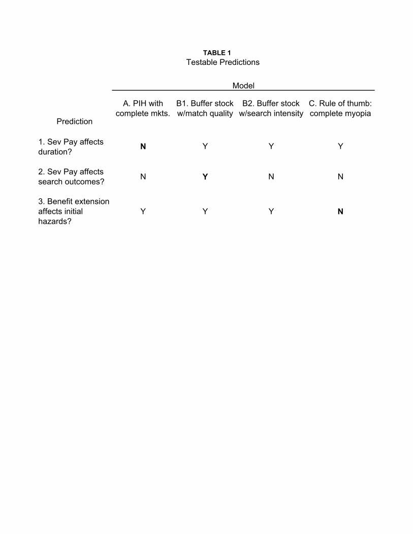
TABLE 1Testable Predictions

Model

Prediction

A. PIH with complete mkts.

B1. Buffer stock w/match quality

B2. Buffer stock w/search intensity

C. Rule of thumb: complete myopia

1. Sev Pay affects duration? N Y Y Y

2. Sev Pay affects search outcomes? N Y N N

3. Benefit extension affects initial hazards?

Y Y Y N

Mean Median Std. Dev.

Worker Characteristics:Age in Years 31.20 30.00 7.96Female 0.52 1.00 0.50Post-compulsory Schooling 0.60 1.00 0.49Married 0.43 0.00 0.50Austrian Citizen 0.88 1.00 0.33Blue Collar Occupation 0.58 1.00 0.49

Previous Job/Employment:Months of Tenure 25.61 21.90 11.93Months Worked in Past 5 Years 41.11 44.10 13.79Eligible for Severance Pay 0.21 0.00 0.41Eligible for Extended UI 0.66 1.00 0.47Previous Wage (Euros/yr) 17033.69 15949.75 7587.71Wage Top-Coded 0.02 0.00 0.14

Post-Layoff:Duration of Unemployment 4.75 2.94 8.37Unemployed < 20 Weeks 0.64 1.00 0.48Unemployed < 52 Weeks 0.94 1.00 0.24Duration of Nonemployment 16.93 4.29 38.19Nonemployed < 20 Weeks 0.51 1.00 0.50Nonemployed < 52 Weeks 0.77 1.00 0.42Observed in New Job 0.92 1.00 0.27

Among those with New Job: Months to Re-employment 8.96 3.84 17.71 Change in Log Wage -0.03 -0.01 0.51

Note: Based on sample of 650,922 job losers over the period 1980-2001. Sample includes people age 20-50 who worked at their previous firm between 1 and 5 years. Job quitters and individuals losing a job in construction are excluded. Wages are expressed in real (year 2000) Euros.

Table 2Sample Characteristics: Austrian Job Losers, 1980-2002

(1) (2) (3) (4) (5)Restricted Restricted Full With Tenure

sample sample sample controls Seasonality

Dependent Var:

Severance pay -0.127 -0.125 -0.115 -0.076(0.019) (0.017) (0.018) (0.019)

Extended benefits -0.084 -0.093 -0.064 -0.065(0.018) (0.016) (0.017) (0.017)

Sample size 512,767 512,767 650,922 565,835 565,835

with interactions with sevpay and/or extended benefit dummy. See text for details.

TABLE 3a

NOTE--All specs are Cox hazard models that include cubic polynomials

Job Finding Hazard

Hazard Model Estimates: Effects of Severance Pay and EB on Durations

(6) (7) (8) (9) (10) (11)Saturated Excluding Unemp. Placebo Placebo Placebocontrols end of year censored no ctrls controls comparison

Severance pay -0.094 -0.095 -0.099 -0.112(0.019) (0.033) (0.022) (0.038)

Extended benefits -0.064 -0.059 -0.078 -0.073(0.018) (0.019) (0.021) (0.058)

Sev. pay placebo -0.017 -0.016 -0.016(0.037) (0.039) (0.037)

EB placebo -0.003 0.009 -0.007(0.024) (0.026) (0.024)

Sample size 509,355 457,783 650,922 122,848 108,383 122,848

with interactions with sevpay and/or extended benefit dummy. See text for details.

TABLE 3bHazard Model Estimates: Effects of Severance Pay and EB on Durations

NOTE--All specs are Cox hazard models that include cubic polynomials

(1) (2) (3) (4)No controls Full controls No controls Full controls

Dependent var: log wage change log wage change job leaving haz. job leaving haz.

Severance pay -0.011 -0.004 -0.023 -0.004(0.006) (0.006) (0.015) (0.017)

Extended benefits -0.005 -0.008 -0.011 0.004(0.005) (0.005) (0.014) (0.015)

coefficients from OLS regressions; columns (3) and (4) report Cox hazard model coefficient estimates.See text for details.

Effects of Severance Pay and EB on Search Outcomes

All specs include cubic polynomials with interactions with sevpay and ebl. Columns (1) and (2) report

TABLE 4

FI PIH B CC CM

FI. Full insurance: PIH with complete markets

PIH. Standard PIH with unrestricted borrowing and lending

B. Buffer stock models (Deaton 1991; Carroll 1992)

CC. Credit constrained: binding asset limit but forward looking

CM. Complete myopia “rule of thumb” with consumption = income

sensitivity to cash-in-hand

m= 0 )

Figure 1Dynamic Models Ordered by Sensitivity to Cash-In-Hand

.4.6

.81

Perc

ent E

ligib

le fo

r 30

Wee

ks o

f UI B

enef

its

12 18 24 30 36 42 48 54 60

Previous Job Tenure (Months)

Eligibility for Extended Benefits by Job Tenure

Figure 2a

0.1

.2.3

.4

Per

cent

Elig

ible

for S

ever

ance

Pay

12 18 24 30 36 42 48 54 60Months Employed in Past Five Years

Eligibility for Severance Pay by Past Employment

Figure 2b

010

000

2000

030

000

4000

0

Num

ber o

f Lay

offs

12 18 24 30 36 42 48 54 60Previous Job Tenure (Months)

Frequency of Layoffs by Job Tenure

Figure 3

3031

3233

34

Mea

n Ag

e

12 18 24 30 36 42 48 54 60Previous Job Tenure (Months)

Age by Job Tenure

Figure 4a

1616

.517

17.5

1818

.5

Mea

n An

nual

Wag

e (E

uro

x 10

00)

12 18 24 30 36 42 48 54 60Previous Job Tenure (Months)

Wage by Job Tenure

Figure 4b

1.05

1.1

1.15

1.2

1.25

Mea

n Pr

edic

ted

Haz

ard

Rat

ios

12 18 24 30 36 42 48 54 60Previous Job Tenure (Months)

Selection on Observables

Figure 4c

145

150

155

160

165

Mea

n N

onem

ploy

men

tDur

atio

n

12 18 24 30 36 42 48 54 60Previous Job Tenure (Months)

Effect of Severance Pay on Nonemployment Durations

Figure 5a

140

145

150

155

160

Mea

n N

onem

ploy

men

tDur

atio

n

12 18 24 30 36 42 48 54 60Previous Job Tenure (Months)

Effect of Severance Pay in Restricted Sample

Figure 5b

-.3-.2

-.10

.1

Aver

age

Dai

ly J

ob F

indi

ng H

azar

d in

Firs

t 20

Wee

ks

12 18 24 30 36 42 48 54 60Previous Job Tenure (Months)

Effect of Severance Pay on Job Finding Hazards

Figure 6a

-.3-.2

-.10

.1

Aver

age

Dai

ly J

ob F

indi

ng H

azar

d in

Firs

t 20

Wee

ks

12 18 24 30 36 42 48 54 60Previous Job Tenure (Months)

Job Finding Hazards Adjusted for Covariates

Figure 6b

-.3-.2

-.10

.1

Aver

age

Dai

ly J

ob F

indi

ng H

azar

d in

Firs

t 20

Wee

ks

12 18 24 30 36 42 48 54 60Previous Job Tenure (Months)

Effect of Severance Pay Adjusted for Tenure Seasonality

Figure 6c

130

140

150

160

170

180

Med

ian

Non

empl

oym

entD

urat

ion

12 18 24 30 36 42 48 54 60Job Tenure in Job Before the One Just Lost (Months)

Placebo Test: Job Tenure and Subsequent Nonemployment Duration

Figure 7

.02

.03

.04

.05

.06

Aver

age

Wee

kly

Job

Find

ing

Haz

ard

0 10 20 30Previous Job Tenure (Months)

No Severance Severance

Effect of Severance Pay on Weekly Job Finding Hazards

Figure 8a

.02

.03

.04

.05

.06

Aver

age

Wee

kly

Job

Find

ing

Haz

ard

0 10 20 30Months Employed in Past Five Years

20 Week UI 30 Week UI

Effect of Extended Benefits on Weekly Job Finding Hazards

Figure 8b

135

140

145

150

155

160

165

Mea

n N

onem

ploy

men

tDur

atio

n

12 18 24 30 36 42 48 54 60Months Employed in Past Five Years

Effect of Benefit Extension on Nonemployment Durations

Figure 9a

135

140

145

150

155

160

165

Mea

n N

onem

ploy

men

tDur

atio

n

12 18 24 30 36 42 48 54 60Months Employed in Past Five Years

Effect of Benefit Extension: Restricted Sample

Figure 9b

-.10

.1.2

Aver

age

Dai

ly J

ob F

indi

ng H

azar

d in

Firs

t 20

Wee

ks

12 18 24 30 36 42 48 54 60Months Employed in Past Five Years

Effect of Extended Benefits on Job Finding Hazards

Figure 9c

Figure 10aEffect of Severance Pay on Wage in Next Job

-.06

-.04

-.02

0.0

2

10 20 30 40 50 60Previous Job Tenure (months)

Log

Cha

nge

in W

age

from

Pre

viou

s Jo

b to

Nex

t

.04

.045

.05

.055

.06

10 20 30 40 50 60

Previous Job Tenure (months)

Figure 10bEffect of Severance Pay on Duration of Next Job

Aver

age

Mon

thly

Haz

ard

in F

irst 2

Yea

rs

Effect of Extended Benefits on Wage in Next JobFigure 11a

Months Employed in Past Five Years

-.05

0.0

5.1

10 20 30 40 50 60Log

Cha

nge

in W

age

from

Pre

viou

s Jo

b to

Nex

t

Figure 11bEffect of Extended Benefits on Duration of Next Job

.046

.048

.05

.052

.054

10 20 30 40 50 60Months Employed in Past Five Years

Aver

age

Mon

thly

Haz

ard

in F

irst 2

Yea

rs