School Attendance, Child Labor and Local Labor Market Fluctuations in Urban Brazil', World...

School Attendance, Child Labor and Local Labor Markets in Urban Brazil

Suzanne DuryeaInter-American Development Bank

[email protected]

Mary Arends-KuenningUniversity of Illinois at Urbana-Champaign

[email protected]

November 2001

Prepared for presentation at the conference “Crises and Disasters: Measurement andMitigation of their Human Costs” organized by the IDB and IFPRI.

This document reflects the opinions of the authors and does not represent the opinions ofthe Inter-American Development Bank or its Board of Directors.

2

Abstract

While the income (poverty) effect on child labor is long established as a maindeterminant of child labor, there is a growing body of literature considering the pull ofthe labor market. This paper demonstrates that ceteris paribus, employment rates for 14-16 year old boys and girls in urban Brazil increase as local labor market opportunitiesimprove. Children are also more likely to leave school as local labor market conditionsbecome more favorable. The effects of aggregate shocks on children’s school and workbehavior are examined with particular focus on whether the income effect or substitutioneffect dominates as macroeconomic conditions change over time. The study uses datafrom the Pesquisa Nacional Amostra de Domicilios, a large household survey that isconducted almost annually by the IBGE. We use variation in the urban areas of 25 statesover 12 years to identify the aggregate effects.

3

Introduction

Recently, researchers have given renewed attention to the issue of child labor,

with lively debates ensuing regarding the causes of child labor. One school of thought is

that child labor is caused primarily by poverty. The looming global recession would be

expected to push children into work and out of school as parent’s incomes fall.

However, some Latin American evidence casts doubt on the hypothesis that child labor is

determined entirely by poverty. In Brazil, and to a lesser extent in other Latin American

countries, evidence exists that rates of child labor are higher at times and in places where

children have better work opportunities as measured by local labor market conditions.

The decision to send children to school is closely related to the decision to send

children to work. The benefits of child labor are related to local labor market conditions.

When children face favorable work conditions, the opportunity costs of schooling

increase. Market work opportunities tend to be better and also more acceptable for boys

than for girls, so that boys face higher opportunity costs of schooling than girls.

Therefore, we examine separately impacts for girls from impacts for boys.

A problem that arises in this literature is the difficulty of distinguishing the

income effects of increased child wages from the substitution effects. Some studies,

discussed in detail below, have found that child wages have a negative impact on child

labor. We are able to distinguish between income and substitution effects by using time-

varying data. The data, the Pesquisa Nacional por Amostra de Domicilios (PNAD), are

repeated cross sections covering the period 1977 to 1998. The sample size is large

enough that we are able to get good aggregate measures of local labor market conditions.

We also distinguish between income and substitution effects of child wages by

comparing regression results that include and exclude controls for household income.

In this paper, we provide a literature review of recent work on child labor and

child schooling, focusing on previous work for Brazil. We also present an overview of

recent trends in child labor and child schooling, showing that child labor has been

decreasing steadily and child schooling has increased since the mid-1990s. The trends

show remarkably variation over time, with peaks in child labor during boom years. We

use bivariate probit models to allow correlations between the decisions to send children

to school and to work, pooling several years of PNAD data. All the models are fully

4

interacted with gender, so that we can carefully examine gender differences in the

determinants of child labor and child schooling, which many previous studies have

neglected to do.

Literature review

Researchers have recognized the importance of opportunity costs in schooling

decisions at least since Gary Becker first wrote about human capital in the 1960s. In

Becker’s analysis, parents want to invest in children’s schooling up to the point where the

marginal cost equals the marginal benefit. Marginal costs of schooling increase as the

child’s market wage increases. In Latin America, empirical evidence suggests that the

opportunity cost of children’s market wages does impact school enrollment. A study by

Jacoby and Skoufias in Peru (1997) found that the child wage has a negative effect on

children’s schooling. The child wage is calculated at the village level as the average

wage of children who work in the market. They did not report results by gender. A study

by Levison, Moe, and Knaul (1999) of child labor and education in Mexico found that the

child wage had a negative effect on the probability that the child would work only, and a

positive effect on the probability that a child would work and attend school, relative to

the child only attending school. The child wage included in the time allocation

regression was estimated using the Heckman procedure to correct for sample selection

bias. The authors acknowledged that the sample selection procedure was problematic,

because the same variables used to estimate the corrected estimated wages were also

determinants of the child allocation decision so that the effect of children’s wages on time

allocation was confounded with other factors.

Whereas a wealth of studies exist regarding the determinants of school attendance

and child labor in particular countries, the lack of degrees of freedom in time varying data

has limited the research on the effects of macroeconomic conditions on children’s time

allocation. In a notable exception, Binder (1999) did a study of schooling in Mexico

during the 1980s using state-level schooling indicators. She used the states’ tax revenues

as a proxy for opportunity costs of schooling, and found a negative relationship between

tax revenues and children’s schooling outcomes. During high revenue times, children

were less likely to attend school. The aggregate level schooling data did not permit

Binder to examine whether boys or girls responded differently. Another limitation of this

5

study was the suitability of state tax revenues as a proxy for children’s labor market

opportunities.

Studies specific to Brazil have also found that labor market opportunities have

impacts on children’s labor supply. Barros et al. (1994) found that the incidence of child

labor tended to be higher in wealthier states than in poorer states and in a short time

series of national data, higher during good economic times than during poor economic

times. For example, child labor was higher in the southern developed state of Sao Paulo

than in the impoverished northern state of Bahia. In a study that looked at child labor

from 1981 to 1996, da Silva Leme and Wajnman (2000) found that when national

unemployment was high, school enrollment increased. The unemployment effect was

interpreted as children being more likely to attend school when it was difficult to find

jobs. However, the study did not find any effect of national wage levels on children’s

attendance. The da Silva Leme and Wajnman paper also did not investigate whether the

effects of wages differed for boys and girls. Neri and Thomas (2001) used the Pesquisa

Mensal do Emprego (PME), which is a short panel of monthly employment data, and

found that child labor was above a fitted trend line during times of economic growth.

Child employment was on the trend line during recessions. The probability that a child

repeated a grade was also above a trend line during times of growth rather than during

recessions. A study by Kassouf (1998) found using the 1995 Pesquisa Nacional por

Amostra de Domicilios (PNAD) data that the higher the child’s estimated log wage, the

less likely the child would be in school. Also, the higher the child’s estimated wage, the

more likely that the child would be employed. The effects of the child’s estimated wage

on schooling and on employment are stronger for boys than for girls. A study by Barros,

Mendonça, Deliberalli, and Bahia (2000) using the 1998 PNAD data found that the

child’s wage had an unexpected negative effect on child employment. The child wage

was measured by taking the average child wage for the municipality. The negative effect

might have resulted because the child wage was a proxy for state income levels. The

study did not look at the impact of the child wage on current school enrollment rates.

Most studies have found that in Brazil, child labor is procyclical, indicating that

opportunity costs have an important impact on children’s schooling.

6

Finally, in the most comprehensive look at opportunity costs to date, Barros,

Mendonça, and Santos (1999) looked at the expected wage as the measure of the

opportunity cost of schooling. The expected wage was defined as the wage of a standard

worker in the local labor market times the probability that a person with the

characteristics of the standard worker would find a job.1 The wage of a standard worker

was defined using regression analysis, predicting a wage for each worker in a

community, and taking the median difference between the actual wage and the predicted

wage as a measure of the labor market situation. This was then multiplied by the

probability of finding work in that community. The outcome variable was years of

schooling, and the analysis focused on children and young adults aged 11 to 25. The

study used the 1996 PNAD and also the Pesquisa Sobre Padroes de Vida 1996–97

(PPV).2 For the PNAD data, opportunity costs were found to have a statistically

significant, negative effect on schooling. Also, males’ response to opportunity costs was

stronger than females’ response to opportunity costs, and the effect was stronger in the

Northeast than in the Southeast. However, the study did not establish for certain that

opportunity costs affected schooling because the analysis using the PPV did not support

the opportunity cost hypothesis. For the PPV, the effect of opportunity costs on

schooling was not statistically significant. Also, the effects of the expected wage on

schooling were marginally statistically significant and positive when the regressions

included measures of access to schooling.

While various papers have examined the effects of aggregate conditions on

schooling and child work in Latin America, none have controlled for individual family

characteristics while permitting time variation in local labor markets. Recognizing that

unobserved heterogeneity at both the individual level and state level is of primary

concern in the estimation procedures, this study aims to answer the question of how

children’s time allocation changes when local labor market conditions change. It also

seeks to address how policy might be linked to different types of aggregate fluctuations.

1 This expected wage was defined in two ways—once using the probability that an unemployed standardworker would get a job and a second time as the probability that an economically active standard workerwould get a job.2 The PPV is considered the World Bank Living Standards Measurement Survey for Brazil.

7

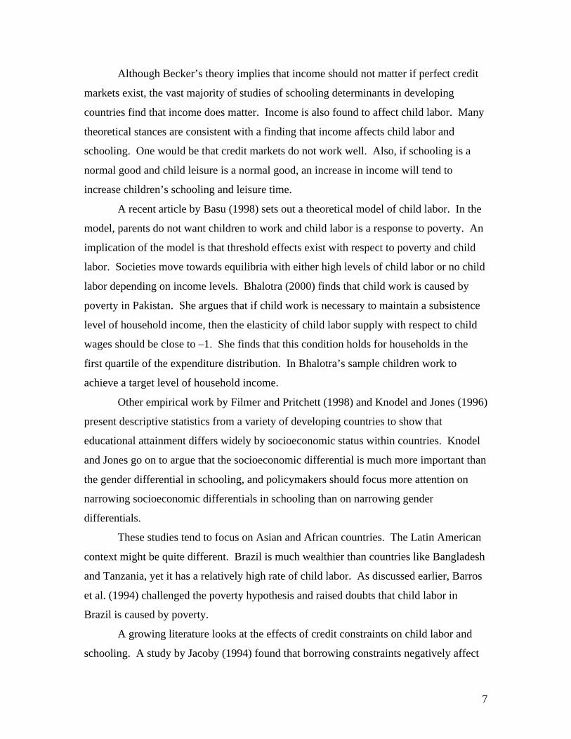
Although Becker’s theory implies that income should not matter if perfect credit

markets exist, the vast majority of studies of schooling determinants in developing

countries find that income does matter. Income is also found to affect child labor. Many

theoretical stances are consistent with a finding that income affects child labor and

schooling. One would be that credit markets do not work well. Also, if schooling is a

normal good and child leisure is a normal good, an increase in income will tend to

increase children’s schooling and leisure time.

A recent article by Basu (1998) sets out a theoretical model of child labor. In the

model, parents do not want children to work and child labor is a response to poverty. An

implication of the model is that threshold effects exist with respect to poverty and child

labor. Societies move towards equilibria with either high levels of child labor or no child

labor depending on income levels. Bhalotra (2000) finds that child work is caused by

poverty in Pakistan. She argues that if child work is necessary to maintain a subsistence

level of household income, then the elasticity of child labor supply with respect to child

wages should be close to –1. She finds that this condition holds for households in the

first quartile of the expenditure distribution. In Bhalotra’s sample children work to

achieve a target level of household income.

Other empirical work by Filmer and Pritchett (1998) and Knodel and Jones (1996)

present descriptive statistics from a variety of developing countries to show that

educational attainment differs widely by socioeconomic status within countries. Knodel

and Jones go on to argue that the socioeconomic differential is much more important than

the gender differential in schooling, and policymakers should focus more attention on

narrowing socioeconomic differentials in schooling than on narrowing gender

differentials.

These studies tend to focus on Asian and African countries. The Latin American

context might be quite different. Brazil is much wealthier than countries like Bangladesh

and Tanzania, yet it has a relatively high rate of child labor. As discussed earlier, Barros

et al. (1994) challenged the poverty hypothesis and raised doubts that child labor in

Brazil is caused by poverty.

A growing literature looks at the effects of credit constraints on child labor and

schooling. A study by Jacoby (1994) found that borrowing constraints negatively affect

8

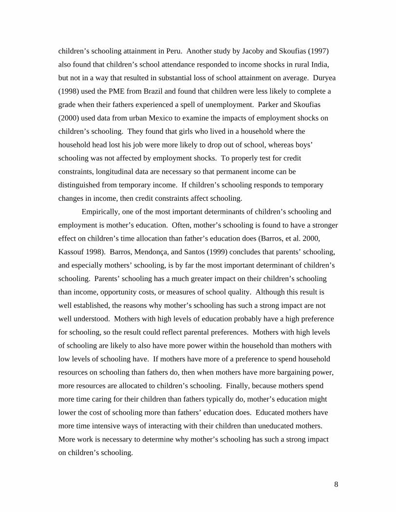
children’s schooling attainment in Peru. Another study by Jacoby and Skoufias (1997)

also found that children’s school attendance responded to income shocks in rural India,

but not in a way that resulted in substantial loss of school attainment on average. Duryea

(1998) used the PME from Brazil and found that children were less likely to complete a

grade when their fathers experienced a spell of unemployment. Parker and Skoufias

(2000) used data from urban Mexico to examine the impacts of employment shocks on

children’s schooling. They found that girls who lived in a household where the

household head lost his job were more likely to drop out of school, whereas boys’

schooling was not affected by employment shocks. To properly test for credit

constraints, longitudinal data are necessary so that permanent income can be

distinguished from temporary income. If children’s schooling responds to temporary

changes in income, then credit constraints affect schooling.

Empirically, one of the most important determinants of children’s schooling and

employment is mother’s education. Often, mother’s schooling is found to have a stronger

effect on children’s time allocation than father’s education does (Barros, et al. 2000,

Kassouf 1998). Barros, Mendonça, and Santos (1999) concludes that parents’ schooling,

and especially mothers’ schooling, is by far the most important determinant of children’s

schooling. Parents’ schooling has a much greater impact on their children’s schooling

than income, opportunity costs, or measures of school quality. Although this result is

well established, the reasons why mother’s schooling has such a strong impact are not

well understood. Mothers with high levels of education probably have a high preference

for schooling, so the result could reflect parental preferences. Mothers with high levels

of schooling are likely to also have more power within the household than mothers with

low levels of schooling have. If mothers have more of a preference to spend household

resources on schooling than fathers do, then when mothers have more bargaining power,

more resources are allocated to children’s schooling. Finally, because mothers spend

more time caring for their children than fathers typically do, mother’s education might

lower the cost of schooling more than fathers’ education does. Educated mothers have

more time intensive ways of interacting with their children than uneducated mothers.

More work is necessary to determine why mother’s schooling has such a strong impact

on children’s schooling.

9

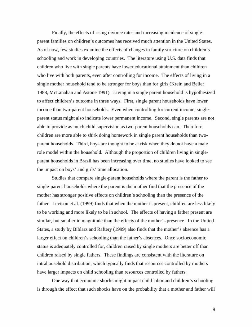
Finally, the effects of rising divorce rates and increasing incidence of single-

parent families on children’s outcomes has received much attention in the United States.

As of now, few studies examine the effects of changes in family structure on children’s

schooling and work in developing countries. The literature using U.S. data finds that

children who live with single parents have lower educational attainment than children

who live with both parents, even after controlling for income. The effects of living in a

single mother household tend to be stronger for boys than for girls (Krein and Beller

1988, McLanahan and Astone 1991). Living in a single parent household is hypothesized

to affect children’s outcome in three ways. First, single parent households have lower

income than two-parent households. Even when controlling for current income, single-

parent status might also indicate lower permanent income. Second, single parents are not

able to provide as much child supervision as two-parent households can. Therefore,

children are more able to shirk doing homework in single parent households than two-

parent households. Third, boys are thought to be at risk when they do not have a male

role model within the household. Although the proportion of children living in single-

parent households in Brazil has been increasing over time, no studies have looked to see

the impact on boys’ and girls’ time allocation.

Studies that compare single-parent households where the parent is the father to

single-parent households where the parent is the mother find that the presence of the

mother has stronger positive effects on children’s schooling than the presence of the

father. Levison et al. (1999) finds that when the mother is present, children are less likely

to be working and more likely to be in school. The effects of having a father present are

similar, but smaller in magnitude than the effects of the mother’s presence. In the United

States, a study by Biblarz and Raftery (1999) also finds that the mother’s absence has a

larger effect on children’s schooling than the father’s absences. Once socioeconomic

status is adequately controlled for, children raised by single mothers are better off than

children raised by single fathers. These findings are consistent with the literature on

intrahousehold distribution, which typically finds that resources controlled by mothers

have larger impacts on child schooling than resources controlled by fathers.

One way that economic shocks might impact child labor and children’s schooling

is through the effect that such shocks have on the probability that a mother and father will

10

stay together. Economic stress tends to increase the likelihood that a marriage will break

up, as the benefits of marriage decrease and uncertainty increases (Becker? ).

Theory

The decision for children to go to work or to school or both is a time allocation

decision. In our case, parents and children decide how to allocate the child’s time and

they agree on the outcome. The decision could also be considered as the outcome of a

bargaining process among parents and children. Estimating a bargaining model would

be very difficult in the absence of information about what happens within households.

We need more information about who actually makes these decisions (mothers, fathers,

or children), and about how to identify bargaining power. There is a well-developed

literature looking at bargaining outcomes between husbands and wives, but to date, no

empirical studies have looked at bargaining outcomes between parents and children or

between mothers, fathers, and children. For simplicity, we assume that the child’s

involvement in work and school is the result of a unitary household decision.

The household decision-maker maximizes a two-period utility function where the

time periods are t and t+1. In the equation below, the household comprises three people:

a father (f), a mother (m) and a child (c).

V = ωf Uft + ωm Umt + ωc Uct + (1+δ)-1 E(ωf Uf,t+1 + ωm Um,t+1 + ωc Uc,t+1)

The decision-maker places weight ω on each member’s utility. The weights can be

thought of as the outcome of a bargaining process. In a single-mother household, ωf is

set to zero, and in a single-father household, ωm is set to zero. Future utility is discounted

by δ, and E represents expectations.

Utility is a function of consumption x, and leisure, l in both periods.

Uit+k = Uit+k (xit+k, lit+k), k = 0, 1

In the model, the child lives in the household in the first period and moves out in

the second period. The household decision-maker decides how much schooling the child

will get in the first period through the time allocation decision. In period t+1, the leisure

and consumption of the child will depend on the child’s wage, wct+1, which in turn

11

depends on the child’s schooling, s. Schooling depends on the amount of time the child

devoted to studying in period t, ls.

cct+1, lct+k = f (wct+1)

wct+1 = w(s)

s = s (ls,ct)

The household decision maker maximizes the utility function subject to the

following budget constraint:

Σ i=f,m,c pxit + Σ i=f,m,c witlit + wctls,ct + (1+r)-1 (Σj=f,m pxj,t+1 + Σ j=f,m wjt+1ljt+1) = (1+r)At + Σ

i=f,m,c witLit + (1+r)-1 Σ j=f,m wjt+1Ljt+1 + Tt+1

The budget constraint is standard except for the Tt+1 term, which represents any transfers

from child to parent. If Tt+1 is positive, the child transfers money to the parents, and if it

is negative, the parent transfers money to the child.

Parents and the child decide how to allocate the child’s time. Children can spend

time in school, doing market work that may or may not be remunerated, doing household

chores, or spending leisure time. In these models, changes in the price of one activity

have complicated effects on other activities. A change in the market wage might increase

or decrease time spent in activities besides work. The effect of a change in the market

wage on schooling will depend on the elasticity of substitution between consumption

goods, leisure time and time spent on household chores.

The amount of time a child spends in school is a function of the wages of parents

and children, prices of consumption, expectations of future wages for educated labor, and

expectations of the transfers a child will make to a parent:

ls = g [wit, p, ωi, E(wct+1), E(Tt+1)]

Family structure such as the presence of a mother and the presence of a father can be

thought of as affecting ω and E(Tt+1). For example, if mothers are more aware of

children’s needs or put a greater weight on their utility than fathers do, then children of

single mothers might have higher schooling than children of single fathers do. Also,

single mothers might have greater expectations that their children will support them in

12

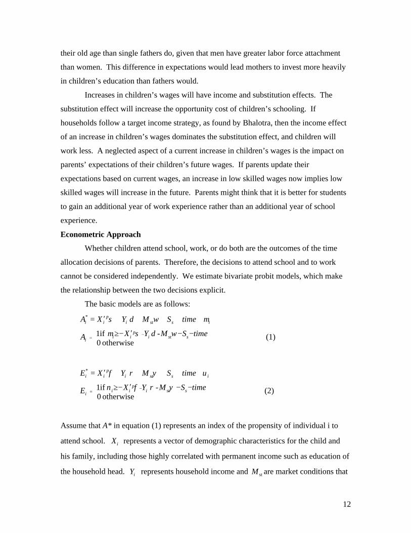
their old age than single fathers do, given that men have greater labor force attachment

than women. This difference in expectations would lead mothers to invest more heavily

in children’s education than fathers would.

Increases in children’s wages will have income and substitution effects. The

substitution effect will increase the opportunity cost of children’s schooling. If

households follow a target income strategy, as found by Bhalotra, then the income effect

of an increase in children’s wages dominates the substitution effect, and children will

work less. A neglected aspect of a current increase in children’s wages is the impact on

parents’ expectations of their children’s future wages. If parents update their

expectations based on current wages, an increase in low skilled wages now implies low

skilled wages will increase in the future. Parents might think that it is better for students

to gain an additional year of work experience rather than an additional year of school

experience.

Econometric Approach

Whether children attend school, work, or do both are the outcomes of the time

allocation decisions of parents. Therefore, the decisions to attend school and to work

cannot be considered independently. We estimate bivariate probit models, which make

the relationship between the two decisions explicit.

The basic models are as follows:

(1) otherwise 0

- if1 =

*

− −−′−≥

+++++′=

timeSMYXA

timeSMYXA

sstip

iii

isstip

ii

ωδσµ

µωδσ

(2) otherwise 0

- if1 =

*

− −−′−≥

+++++′=

timeSMYXE

timeSMYXE

sstip

iii

isstip

ii

ψρφν

υψρφ

Assume that A* in equation (1) represents an index of the propensity of individual i to

attend school. X i represents a vector of demographic characteristics for the child and

his family, including those highly correlated with permanent income such as education of

the household head. iY represents household income and stM are market conditions that

13

are widely available to all individuals in state S at time T. sS are constant terms

representing the 25 states. iµ is a normally and independently distributed error term. A*

is treated as a latent variable and the probability of attending school is modeled as a

probit such that if A* exceeds an unobservable threshold the child is observed attending

school.

Employment is assumed to be a function of the same variables. We estimate

equations 1 and 2 using a bivariate probit regression, which allows us to analyze the

correlation of the error terms in the school attendance and employment equations.

All of the variables are interacted with a male dummy variable. Demographic

characteristics of the family include the age and gender of the child, and the education of

the household head. Whether the individual is listed as the child of the head is also

measured as well as whether the child’s mother or father is absent from the household.3

Since children are assumed to be secondary workers, the per capita income of the family

includes only incomes of those above the age of 18. If demographic characteristics such

as education are excellent proxies for permanent income, then Y will be largely reflecting

transitory income. Our regressions will consider different proxies for M, the

contemporaneous aggregate conditions in the local labor market that capture the

opportunity costs of attending school. Primarily we consider the wages of low skilled

men, represented by the average wage of men aged 30 to 35 with less than 4 years of

schooling who live in state s. We also consider the wages of low skilled women as well

as the state-level per capita income. Even if the wage that children actually earn is less

than the unskilled wage, differences across states and over time are likely to be similar

for the child wage and for the unskilled wage; we are assuming that they move in a

similar fashion because they are determined by the same circumstances. The equation

does not take into account state-level unemployment rates because in Brazil,

unemployment is not a good indicator of macroeconomic conditions. Neri and Thomas

(2000) find that transitions from employment to unemployment are equally likely to

happen during boom times as during recessions, because workers can afford to search for

better jobs rather than to enter into the informal sector immediately after a job loss. They

14

note that the link between poverty and unemployment is tenuous, although it has been

increasing over time.

Basic Trends

(The text and figures showing that trends in wages and child labor and schooling

varies across states will be ready by the conference.)

Results (right now just concentrating on key variables – later will elaborate other interesting results)

Table X1 shows the results of the bivariate probit model estimation using a

standard specification that omits state-level wage variables. Per capita household income

(for adults) significantly raises the probability of attending school and significantly

reduces the probability of being employed. This is the typical finding from micro-data –

children in poorer household are more likely to be working. Extrapolating these results

to declines in the macroeconomic environment suggests that children would work more

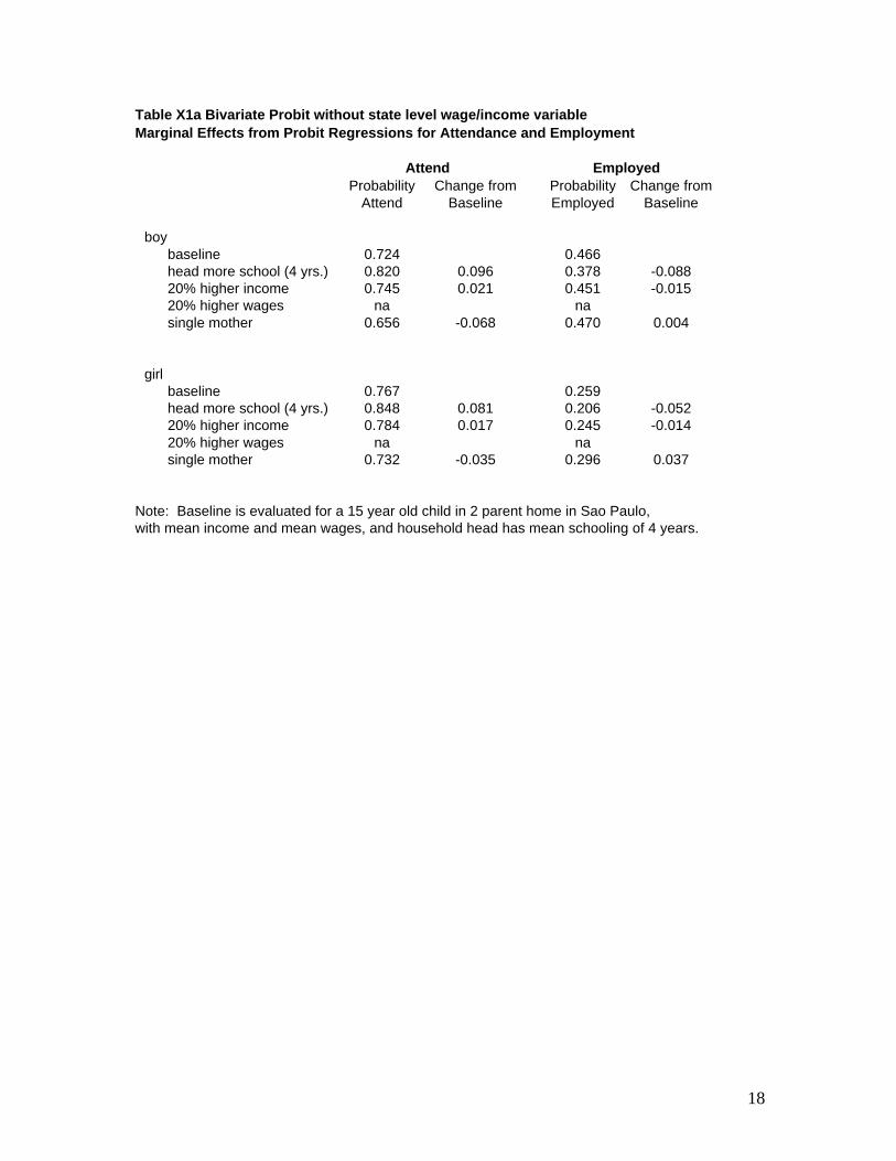
in recessions, e.g., work by children/youths is counter-cyclical. Table X1a presents the

marginal results from this specification. A 20% increase in per capita adult income is

associated with a reduction in child labor of 1.5 percentage points and an increase in the

probability of school attendance by approximately 2 percentage points. Boys’ schooling

is slightly more responsive to the change in income than girls’ schooling, but in general

the marginal effects of income do not vary much by gender.

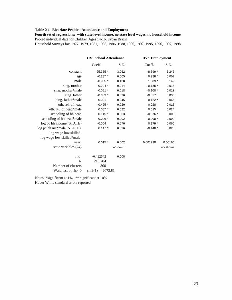
Because the identification of the change in income is coming from largely cross-

sectional comparisons, one may be concerned about biases arising from unobserved

heterogeneity. In other words, it is not surprising that parents with higher income are

more likely to have children in school if unobservables such as tastes for education are

correlated with income. So our next specification in Table X2 omits the per capita

household income at the individual level and instead uses state-time variation in the

wages of low-skilled males to proxy for the macroeconomic environment. Because the

regressions include state level dummy variables, the changes in the unskilled wage over

time within each state are used to identify the effects of opportunity costs on children’s

3 We prefer this specification to the gender of the head because many children are living in extendedfamilies with male heads even though a father (i.e., mother’s spouse) is absent from the household register.

15

schooling. Therefore, we are controlling for the average difference in unskilled wage

across states. Barros et al. (2000) discussed the peculiar finding that children’s wages

had a negative effect on the probability that children would work, and argued that the

wage might be picking up the differences in wealth across areas. An advantage of using

several years of data is that by adding state dummy variables, the regression controls for

differences in wealth across states.

An increase in the low skilled wage will increase the adults’ income as well as the

children’s income. Even households with highly skilled adult workers experience an

income effect during boom times, because good years for low skilled workers are also

likely to be good for highly skilled workers. Table X2 shows that when wages rise, the

probability of working increases – i.e., that youth work is pro-cyclical, with girls being

significantly more responsive to changes in local wages than boys. The gender

differences in the estimates are striking in comparison to the first estimates. Perhaps girls

and boys are treated and/or react similarly to changes in family income but respond or are

treated differently with respect to labor market opportunities.

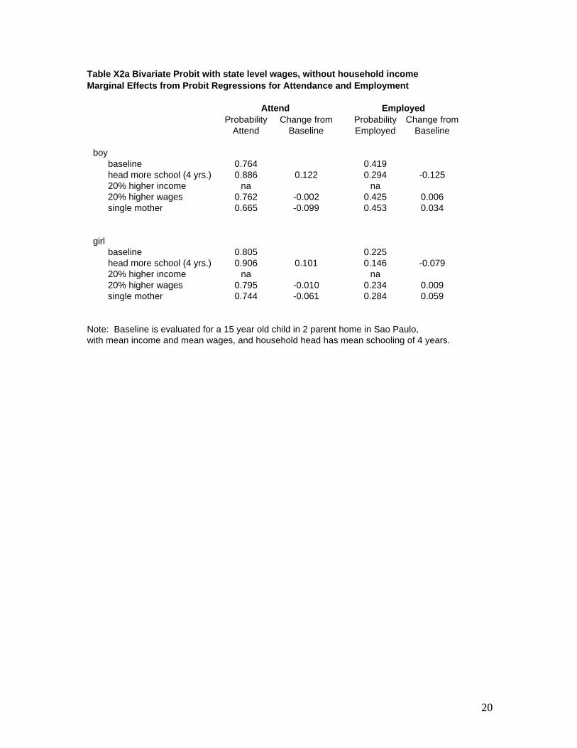
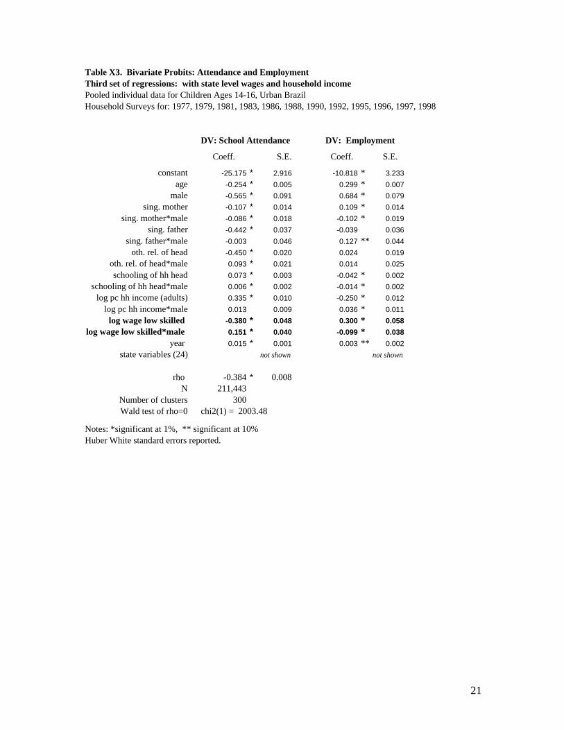
Our third set of estimations uses both the state-level wages as well as the per

capita household income at the individual level. Although the other specifications merely

suggested that child work was mildly pro or counter cyclical, this specification suggests

that the income effect and substitution effect are both relevant for the time allocation of

children. The magnitude of the state-level variables double and the magnitude of the

household level income also increases. The marginal effects shown in Table X3a show

the potentially offsetting effects of changes in labor market conditions. If one controls

for the changes to adult family income, then children’s labor market participation

increases with labor market opportunities.4 (Our results are robust to using the average

wages of prime-age males as well as low-skilled females. Girls are to a larger degree

4 Changes in household income are endogenous responses to economic shocks,

because household income is a function of wages and of hours worked by adulthousehold members. To the extent that women work in response to a negative shock, andchildren’s time allocation is affected by mothers’ time allocation, changes in householdincome will be endogenous to the school and child work decision. We could consider theregression without household income as a “reduced form.”

16

more responsive than boys to the female income. The results are also robust to lowering

the younger age group to 13 to 15.)

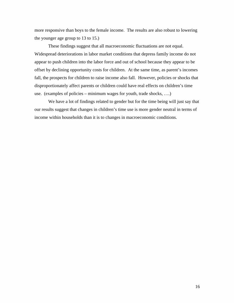
These findings suggest that all macroeconomic fluctuations are not equal.

Widespread deteriorations in labor market conditions that depress family income do not

appear to push children into the labor force and out of school because they appear to be

offset by declining opportunity costs for children. At the same time, as parent’s incomes

fall, the prospects for children to raise income also fall. However, policies or shocks that

disproportionately affect parents or children could have real effects on children’s time

use. (examples of policies – minimum wages for youth, trade shocks, ….)

We have a lot of findings related to gender but for the time being will just say that

our results suggest that changes in children’s time use is more gender neutral in terms of

income within households than it is to changes in macroeconomic conditions.

17

Table X1. Bivariate Probits: Attendance and Employment First set of regressions: without any state level wage/income variablesPooled individual data for Children Ages 14-16, Urban BrazilHousehold Surveys for: 1977, 1979, 1981, 1983, 1986, 1988, 1990, 1992, 1995, 1996, 1997, 1998

DV: School Attendance DV: Employment

Coeff. S.E. t P>|z| Coeff. S.E.

constant -29.321 * 2.944 -9.960 0.000 -7.154 ** 3.238

age -0.253 * 0.005 -50.110 0.000 0.299 * 0.007male -0.276 * 0.044 -6.330 0.000 0.493 * 0.047

sing. mother -0.109 * 0.014 -7.570 0.000 0.111 * 0.014sing. mother*male -0.085 * 0.018 -4.630 0.000 -0.101 * 0.019

sing. father -0.439 * 0.037 -12.010 0.000 -0.040 0.036

sing. father*male -0.004 0.046 -0.090 0.931 0.127 * 0.044oth. rel. of head -0.443 * 0.020 -22.680 0.000 0.020 0.019

oth. rel. of head*male 0.087 * 0.021 4.120 0.000 0.018 0.025schooling of hh head 0.075 * 0.003 28.480 0.000 -0.043 * 0.002

schooling of hh head*male 0.005 ** 0.003 2.140 0.032 -0.013 * 0.002

log pc hh income (adults) 0.319 * 0.010 32.660 0.000 -0.238 * 0.011

log pc hh income*male 0.027 * 0.009 2.830 0.005 0.027 * 0.010

log wage low skilledlog wage low skilled*male

year 0.016 * 0.001 10.970 0.000 0.001 * 0.002

state variables (24) not shown not shown

rho -0.386 * 0.0078N 211,443

Number of clusters 300Wald test of rho=0 chi2(1) = 1959.89 Prob > chi2 = 0.0000

Notes: *significant at 1%, ** significant at 10%Huber White standard errors reported.

18

Table X1a Bivariate Probit without state level wage/income variableMarginal Effects from Probit Regressions for Attendance and Employment

Attend EmployedProbability Change from Probability Change from

Attend Baseline Employed Baseline

boybaseline 0.724 0.466head more school (4 yrs.) 0.820 0.096 0.378 -0.08820% higher income 0.745 0.021 0.451 -0.01520% higher wages na nasingle mother 0.656 -0.068 0.470 0.004

girlbaseline 0.767 0.259head more school (4 yrs.) 0.848 0.081 0.206 -0.05220% higher income 0.784 0.017 0.245 -0.01420% higher wages na nasingle mother 0.732 -0.035 0.296 0.037

Note: Baseline is evaluated for a 15 year old child in 2 parent home in Sao Paulo,with mean income and mean wages, and household head has mean schooling of 4 years.

19

Table X2. Bivariate Probits: Attendance and Employment Second set of regressions: with state level wages, without household incomePooled individual data for Children Ages 14-16, Urban BrazilHousehold Surveys for: 1977, 1979, 1981, 1983, 1986, 1988, 1990, 1992, 1995, 1996, 1997, 1998


Coeff. S.E. Coeff. S.E.

constant -24.033 * 3.028 -10.105 * 3.231

age -0.237 * 0.005 0.288382 * 0.00664

male -0.545 * 0.085 0.760 * 0.075

sing. mother -0.204 * 0.014 0.184 * 0.013

sing. mother*male -0.090 * 0.018 -0.098 * 0.018

sing. father -0.383 * 0.036 -0.057 0.036

sing. father*male 0.000 0.045 0.122 0.045

oth. rel. of head -0.425 * 0.020 0.025 0.018

oth. rel. of head*male 0.086 * 0.022 0.020 0.024

schooling of hh head 0.114 * 0.003 -0.075 * 0.003

schooling of hh head*male 0.008 * 0.002 -0.010 * 0.002

log pc hh income (adults)log pc hh income*male

log wage low skilled -0.195 * 0.041 0.155 * 0.052log wage low skilled*male 0.162 * 0.038 -0.074 ** 0.034

year 0.014 * 0.002 0.002 0.002


rho -0.412 0.008

N 218,784Number of clusters 300Wald test of rho=0 chi2(1) = 2075.57


20

Table X2a Bivariate Probit with state level wages, without household incomeMarginal Effects from Probit Regressions for Attendance and Employment



boybaseline 0.764 0.419head more school (4 yrs.) 0.886 0.122 0.294 -0.12520% higher income na na20% higher wages 0.762 -0.002 0.425 0.006single mother 0.665 -0.099 0.453 0.034

girlbaseline 0.805 0.225head more school (4 yrs.) 0.906 0.101 0.146 -0.07920% higher income na na20% higher wages 0.795 -0.010 0.234 0.009single mother 0.744 -0.061 0.284 0.059


21

Table X3. Bivariate Probits: Attendance and Employment Third set of regressions: with state level wages and household incomePooled individual data for Children Ages 14-16, Urban BrazilHousehold Surveys for: 1977, 1979, 1981, 1983, 1986, 1988, 1990, 1992, 1995, 1996, 1997, 1998



constant -25.175 * 2.916 -10.818 * 3.233

age -0.254 * 0.005 0.299 * 0.007male -0.565 * 0.091 0.684 * 0.079

sing. mother -0.107 * 0.014 0.109 * 0.014

sing. mother*male -0.086 * 0.018 -0.102 * 0.019sing. father -0.442 * 0.037 -0.039 0.036

sing. father*male -0.003 0.046 0.127 ** 0.044

oth. rel. of head -0.450 * 0.020 0.024 0.019oth. rel. of head*male 0.093 * 0.021 0.014 0.025

schooling of hh head 0.073 * 0.003 -0.042 * 0.002schooling of hh head*male 0.006 * 0.002 -0.014 * 0.002

log pc hh income (adults) 0.335 * 0.010 -0.250 * 0.012

log pc hh income*male 0.013 0.009 0.036 * 0.011

log wage low skilled -0.380 * 0.048 0.300 * 0.058

log wage low skilled*male 0.151 * 0.040 -0.099 * 0.038

year 0.015 * 0.001 0.003 ** 0.002state variables (24) not shown not shown

rho -0.384 * 0.008N 211,443

Number of clusters 300Wald test of rho=0 chi2(1) = 2003.48


22

Table X3a Bivariate Probit: with state level wages and household incomeMarginal Effects from Probit Regressions for Attendance and Employment



boybaseline 0.754 0.436head more school (4 yrs.) 0.842 0.088 0.350 -0.08520% higher income 0.774 0.020 0.421 -0.01520% higher wages 0.741 -0.013 0.450 0.014single mother 0.690 -0.064 0.439 0.003

girlbaseline 0.794 0.235head more school (4 yrs.) 0.867 0.073 0.187 -0.04820% higher income 0.811 0.017 0.221 -0.01420% higher wages 0.774 -0.020 0.252 0.017single mother 0.762 -0.032 0.270 0.035


23

Table X4. Bivariate Probits: Attendance and Employment Fourth set of regressions: with state level income, no state level wages, no household incomePooled individual data for Children Ages 14-16, Urban BrazilHousehold Surveys for: 1977, 1979, 1981, 1983, 1986, 1988, 1990, 1992, 1995, 1996, 1997, 1998



constant -25.365 * 3.062 -8.899 * 3.246

age -0.237 * 0.005 0.288 * 0.007

male -0.965 * 0.138 1.389 * 0.149

sing. mother -0.204 * 0.014 0.185 * 0.013

sing. mother*male -0.091 * 0.018 -0.100 * 0.018

sing. father -0.383 * 0.036 -0.057 0.036

sing. father*male -0.001 0.045 0.122 * 0.045

oth. rel. of head -0.425 * 0.020 0.028 0.018

oth. rel. of head*male 0.087 * 0.022 0.015 0.024

schooling of hh head 0.115 * 0.003 -0.076 * 0.003

schooling of hh head*male 0.006 * 0.002 -0.008 * 0.002

log pc hh income (STATE) -0.064 0.070 0.179 * 0.065

log pc hh inc*male (STATE) 0.147 * 0.026 -0.148 * 0.028

log wage low skilledlog wage low skilled*male

year 0.015 * 0.002 0.001298 0.00166


rho -0.412542 0.008

N 218,784Number of clusters 300Wald test of rho=0 chi2(1) = 2072.81


24

References

Arends-Kuenning, Mary and Sajeda Amin. 2000. “Effects of Schooling IncentivePrograms on Household Time Allocation,” in Policies and Strategies for Womenin the Age of Economic Transformation, edited by G. Summerfield, S. Pressman,and N. Aslanbeigui, Routledge Press

Barros, Ricardo, Rosane Mendonça, Priscila Pereira Deliberalli, and Monica Bahia. 2000.“O trabalho domestico infanto-juvenil no Brasil.” Unpublished paper, Instituto dePesquisa Econômica Aplicada.

Barros, Ricardo, Rosane Mendonça, and Daniel Santos. 1999. “Determinantes dodesempenho educacional no Brasil,” Unpublished paper, Instituto de PesquisaEconômica Aplicada, April.

Barros, Ricardo, Rosane Mendonça, and T. Velazco. 1994. “Is poverty the main cause ofchild work in urban Brazil?” Rio de Janeiro, Texto para Discussão No. 351,Instituto de Pesquisa Econômica Aplicada.

Basu, Kaivak. 1998. “Child labor: Cause, consequence, and cure, with remarks oninternational labor standards.” Journal of Economic Literature, Vol. 37, pp.1083–1119.

Becker, Gary. 1975. Human Capital. Chicago, IL: University of Chicago Press.

Biblarz, Timothy and Adrian Raftery. 1999. “Family structure, educational attainment,and socioeconomic success: Rethinking the pathology of matriarchy.” AmericanJournal of Sociology, Vol. 105, pp. 321–365.

Binder, Melissa. 1999. “Schooling indicators during Mexico’s ‘Lost decade’.” Economicsof Education Review, Vol. 18, pp. 183–199.

da Silva Leme, Maria Carolina and Simone Wajnman. 2000. “A alocação do tempo dosadolescentes brasileiros entre o trabalho e a escola.” Unpublished paper,Universidade do São Paulo.

Duryea, Suzanne. 1998. “Children’s advancement through school in Brazil: The role oftransitory shocks to household income.” Office of the Chief Economist WorkingPaper No. 376. Washington, DC: Interamerican Development Bank

Filmer, Deon and Lant Pritchett. 1998. “The effect of household wealth on educationalattainment.” Policy Research Working Paper No. 1980. Washington, DC: TheWorld Bank.

25

FIPE–USP. 2000. Adolescents in Latin America and the Caribbean: Examining timeallocation decisions with cross-country micro data.” Report to the Inter-AmericanDevelopment Bank Research Network, April.

Hanushek, Eric A. 1992. “The Trade-off between child quantity and quality.” Journal ofPolitical Economy, Vol. 100, No. 1, pp. 84–117.

Jacoby, Hanan. 1993. “Shadow Wages and Peasant Family Labor Supply: AnEconometric Application to the Peruvian Sierra,” Review of Economic Studies,Vol. 60, pp. 903–921.

Jacoby, Hanan and Emmanuel Skoufias. 1997. “Risk, financial markets and humancapital in a developing country.” Review of Economic Studies, Vol. 64, pp. 311–335.

Kassouf, Ana Lucia. 1998. “Child labor in Brazil.” Unpublished paper, Department ofEconomics, London School of Economics, November.

Knodel, John, Napaporn Havanon and Werasit Sittitra. 1990. “Family size and theeducation of children in the context of rapid fertility decline.” Population andDevelopment Review, Vol. 16, No. 1, pp. 31–62.

Knodel, John and Ronald Jones. 1996. “Post-Cairo population policy: Does promotinggirls’ schooling miss the mark?” Population and Development Review. Vol. 22,No. 4, pp. 683–702.

Krein, Sheila and Andrea Beller. 1988. “Educational attainment of children from single-parent families: Differences by exposure, gender, and race.” Demography, Vol.25, No. 2, pp. 221–234.

Levison, Deborah, Karine Moe and Felicia Knaul. 1999. “Youth education and work inMexico.” Paper presented at the Population Association of America annualmeetings, New York.

McLanahan, Sara and Nan Astone. 1991. “Family structure, parental practices and highschool completion.” American Sociological Review, Vol. 56, pp. 309–320.

Montgomery, Mark, Mary Arends-Kuenning, and Cem Mete. 2000. “The quantity-quality tradeoff in Asia,” in Population Change in Asia: Transition, Development,and Aging, edited by C. Chu and R. Lee, supplement to Population andDevelopment Review Vol. 26.

Montgomery, Mark and Aka Kouame. 1994. “Fertility and Child Schooling in Coted’Ivoire: Is There a Tradeoff?” Paper presented at the Northeast UniversitiesDevelopment Conference, Yale University.

26

Parker, Susan. 2000. “School and work in rural marginated communities of Mexico:Evidence from Progresa.” paper presented at the Population Association ofAmerica annual meetings, Los Angeles, CA.

Parker, Susan and Emmanuel Skoufias. 2000. “Parental unemployment, marital statuschanges and child human capital: Evidence from urban Mexico.” Unpublishedmanuscript, Mexico, DF: Progresa.

Patrinos, Harry and George Psacharopoulos. 1997. “Family size, schooling and childlabor in Peru— an empirical analysis.” Journal of Population Economics. Vol.10, No. 4, pp. 387–406.

Psacharopoulos, George. 1997. “Child labor versus educational attainment: Someevidence from Latin America.” Journal of Population Economics. Vol. 10, No. 4,pp. 377–386.

Ravallion, Martin and Quentin Wodon. 1999. “Does Child Labor Displace Schooling?Evidence on Behavioral Responses to an Enrollment Subsidy.” World BankPolicy Research Working Paper No. 2116. Washington, DC: The World Bank.

School Attendance, Child Labor and Local Labor Market Fluctuations in Urban Brazil', World...

Documents

Transcript of School Attendance, Child Labor and Local Labor Market Fluctuations in Urban Brazil', World...