VARIATIONAL MODELS FOR PEELING PROBLEMS

FRANCESCO MADDALENA, DANILO PERCIVALE

Abstract. We study variational models for flexural beams and platesinteracting with a rigid substrate through an adhesive layer. The generalstructure of the minimizers is investigated and some properties charac-terizing the behavior of the systems in dependence of the load and thematerial stiffnesses are discussed.

Contents

Introduction 11. Preliminaries and notation 22. Peeling of elastic beams 32.1. Structure of the minimizers 42.2. Growth conditions and stability analysis 72.3. General load conditions 92.4. Local Minimizers 103. Peeling of elastic plates 13References 18

Introduction

Adhesion phenomena constitute a very challenging area of research fromboth the theoretical and applied points of view. The physics underlyingthe adhesion crucially depends on the properties at the microscale levelof the material constituting the adhesive (usually polymers in the case ofartificial adhesives) and the properties of the surfaces of the jointed bodies.In recent years the instances posed by the miniaturization technology, as inthe case of microelectromechanical systems (MEMS) (see the review [16])or, more in general by nanotechnology, as well as the understanding of the

Date: April 18, 2007.1

2 PEELING

role played by adhesion and elasticity in biophysics (see [6], [10], [5]) havepointed out the need of rational accurate models capturing the essentialsof the complex phenomenologies involved in the adhesion problems. At themacroscopic level the energetic of peeling off a deformable material bodyfrom a rigid (i.e. another material body assumed to be rigid) substrateincorporates an adhesion energy and an elastic energy. Indeed, starting fromthe essential analysis of J. Eriksen carried in [3, Chapter 7.3], the problemof peeling of a thin (extensible or inextensible) tape has been investigated inthe context of continuum mechanics by using a variational formulation (see[13], [4], [2]) and, more recently also the dynamics of these phenomena hasbeen investigated (see [12]). Much of these works assume a membrane likebehavior for the elastic body and consider the adhesion energy as a linearfunction of the measure of the detached zone.

In this paper we study, in the classical setting of Calculus of Variations,the peeling problem for flexural elastic beams and plates. In particular, weconsider a linear elastic behavior in the hypotheses of Bernoulli-Navier andKirchhoff-Love for beams and plates, respectively and we assume the adhe-sion energy is modeled by a continuous monotone function of the measureof the detached zone. In the case of the elastic beams we get a detailedcharacterization of the structure of the minimizers which allows to studythe quasistatic evolution of the system when a monotone increasing loadis supposed to act. In the case of the elastic plates we get two key esti-mates which characterize the regimes of the system in which the plate iscompletely detached or completely bonded, in dependence of the value ofthe load. In both the problems it is seen that a crucial role is played by thegrowth exponent affecting the constitutive assumption characterizing theadhesive material, which can be thought as synthesizing the macroscopiccounterpart of the peculiarities at the microscale. Indeed, different choicesof such an exponent lead to different behaviors of the system.

1. Preliminaries and notation

In this paper H2(Ω) will denote the Sobolev space of the functionsu : Ω → R whose weak second partial derivatives are in L2(Ω). Moreover, letBV (Ω) be the space of the functions with bounded variation, i.e. u ∈ L1(Ω)whose partial derivatives in the sense of distributions are measures withfinite total variation in Ω (see [1], [9]). Now we recall that the perimeterPΩ(E) of a set E relative to Ω is defined as the total variation of the measure

PEELING 3

D1E∩Ω, where 1E∩Ω denotes the characteristic function of the set E ∩ Ω.Finally, we introduce the perimeter of E relative to the closed set R2 \ Ω,namely

PR2\Ω(E) = infPG(E) : G open,R2 \ Ω ⊂ G.

2. Peeling of elastic beams

In the following we shall consider the case of linearly elastic flexuralbeam, in the Bernoulli-Navier hypothesis, interacting with a rigid substratethrough a thin adhesion layer. Let the beam occupy the interval [0, L] in itsreference configuration and let u : [0, L] → R be the displacement functionmeasuring the vertical deflection of the beam. The elastic potential energyis given by

We(u) =1

2

∫ L

0

kb |u′′|2 dx, (1)

where kb = EI denotes the flexural rigidity of the beam, where E is theYoung modulus and I is the inertia moment of the cross section. In orderto model the energetic of the adhesion between the beam and the rigidsubstrate let us introduce the set

Σu = x ∈ [0, L] |u(x) > 0

and let |Σu| be the Lebesgue measure of Σu. We define the adhesion potentialas

Wa(u) = ϑ(L−1|Σu|), (2)

where ϑ : R+ → R is assumed to be continuous and monotone increasingwith ϑ(0) = 0. Let us assume the beam is subjected to a given load fapplied at the right end x = L. Then the load potential takes the form

Wl(u) = −fu(L). (3)

Therefore the total thermodynamic potential is given by

F(u) = We(u) +Wa(u) +Wl(u)

and so, according to the Gibbs Principle, stable equilibrium configurationsof the beam are minimizers of the functional

F(u) =1

2

∫ L

0

kb |u′′|2 dx+ ϑ(L−1|Σu|)− fu(L) (4)

4 PEELING

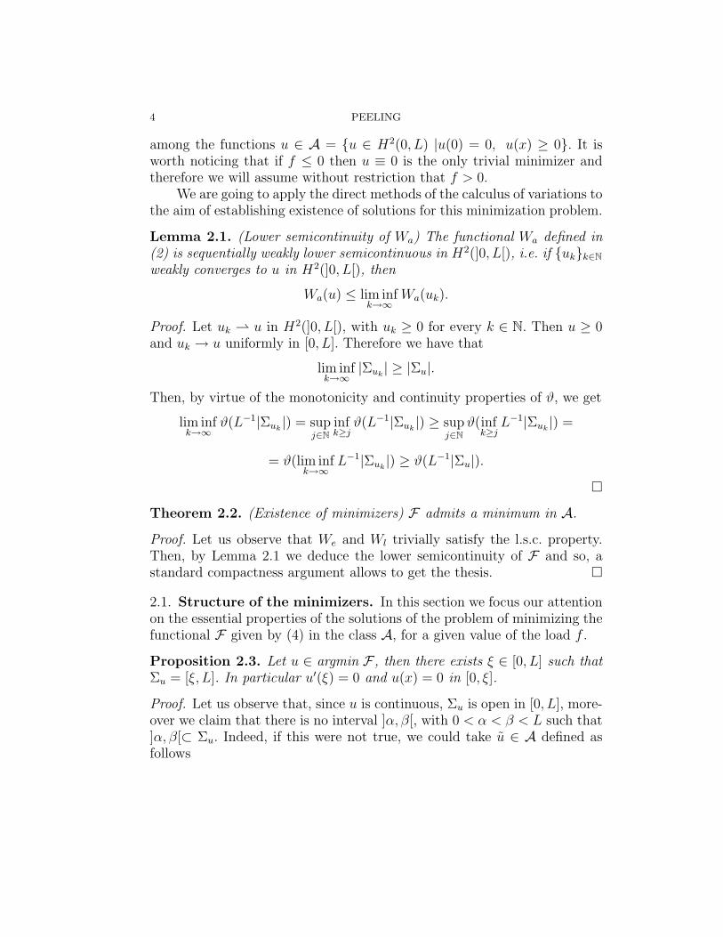
among the functions u ∈ A = u ∈ H2(0, L) |u(0) = 0, u(x) ≥ 0. It isworth noticing that if f ≤ 0 then u ≡ 0 is the only trivial minimizer andtherefore we will assume without restriction that f > 0.

We are going to apply the direct methods of the calculus of variations tothe aim of establishing existence of solutions for this minimization problem.

Lemma 2.1. (Lower semicontinuity of Wa) The functional Wa defined in(2) is sequentially weakly lower semicontinuous in H2(]0, L[), i.e. if ukk∈Nweakly converges to u in H2(]0, L[), then

Wa(u) ≤ lim infk→∞

Wa(uk).

Proof. Let uk u in H2(]0, L[), with uk ≥ 0 for every k ∈ N. Then u ≥ 0and uk → u uniformly in [0, L]. Therefore we have that

lim infk→∞

|Σuk| ≥ |Σu|.

Then, by virtue of the monotonicity and continuity properties of ϑ, we get

lim infk→∞

ϑ(L−1|Σuk|) = sup

j∈Ninfk≥j

ϑ(L−1|Σuk|) ≥ sup

j∈Nϑ(inf

k≥jL−1|Σuk

|) =

= ϑ(lim infk→∞

L−1|Σuk|) ≥ ϑ(L−1|Σu|).

Theorem 2.2. (Existence of minimizers) F admits a minimum in A.

Proof. Let us observe that We and Wl trivially satisfy the l.s.c. property.Then, by Lemma 2.1 we deduce the lower semicontinuity of F and so, astandard compactness argument allows to get the thesis.

2.1. Structure of the minimizers. In this section we focus our attentionon the essential properties of the solutions of the problem of minimizing thefunctional F given by (4) in the class A, for a given value of the load f .

Proposition 2.3. Let u ∈ argmin F , then there exists ξ ∈ [0, L] such thatΣu = [ξ, L]. In particular u′(ξ) = 0 and u(x) = 0 in [0, ξ].

Proof. Let us observe that, since u is continuous, Σu is open in [0, L], more-over we claim that there is no interval ]α, β[, with 0 < α < β < L such that]α, β[⊂ Σu. Indeed, if this were not true, we could take u ∈ A defined asfollows

PEELING 5

u(x) =

u(x) if x ∈ [0, L]\]α, β[

0 if x ∈]α, β[,

to obtain the inequality F(u) < F(u), which yields a contradiction since uis a minimizer. Finally, u′(ξ) = 0 since u ∈ H2(]0, L[).

The previous results allow to state that if u ∈ A minimizes F then itcan be completely characterized in a form which depends on the detachmentvariable ξ, as we are going to prove in the following theorem.

Theorem 2.4. Let u ∈ argmin F then

u(x) =f

kb

(x− ξ

)2(−x

6+L

2− ξ

3

), (5)

where ξ is a global minimizer of

F (ξ) = ϑ

(1− ξ

L

)− f 2L3

6kb

(1− ξ

L

)3

. (6)

Proof. If u ∈ argminF then by Proposition 2.3, the total energy takes theform

F(u) =1

2

∫ L

ξ

kb |u′′|2 dx+ ϑ(1− ξ

L)− fu(L). (7)

Then u minimizes

1

2

∫ L

ξ

kb |v′′|2 dx− fv(L) (8)

among all v ∈ H2(ξ, L) such that v ≥ 0, v(ξ) = v′(ξ) = 0. By taking intoaccount that f > 0, it is readily seen that any minimizer of (7) among allv ∈ H2(ξ, L) such that v(ξ) = v′(ξ) = 0 is greater or equal to zero andtherefore standard first variation of (7) shows that

v′′′′(x) = 0 ∀x ∈]ξ, L[v(ξ) = v′(ξ) = 0,

v′′(L) = 0, v′′′(L) = − f

kb.

(9)

6 PEELING

It is easy to check that the unique solution u of (9) is given by

u(x) =f

kb(x− ξ)2

(−x

6+L

2− ξ

3

). (10)

By substituting (10) in (7) we obtain the minimum energy in dependenceof the free boundary ξ ∈ [0, L], that is

F (ξ) = F(u) = ϑ

(1− ξ

L

)− f 2L3

6kb

(1− ξ

L

)3

(11)

hence

minF = minF (ξ) | ξ ∈ [0, L] (12)

thus completing the proof.

Then, a complete understanding of the analytical properties of the en-ergy minimizers lead to study the minimization problem

minF (ξ) | ξ ∈ [0, L]. (13)

and the value of ξ minimizing F fully characterizes the detachment regionΣu = [ξ, L], for a given value of the load f .

For the sake of convenience and to simplify notations, we introducethe normalized variable ζ =

(1− ξ

L

)and so, after changing variable, (11)

becomes

G(ζ) = ϑ(ζ)− f 2L3

6kbζ3, (14)

with ζ ∈ [0, 1].Since the uniqueness of ζ minimizing G given by (14) depends on the

constitutive choice of the adhesion potential ϑ, we spend a few words con-cerning such uniqueness question. Obviously, strict convexity of G leadsto uniqueness of the minimum ζ. Otherwise, different choices of ϑ lead tomultiple minima. Indeed, if for instance we take

ϑ(ζ) =f 2L3

6kb

(ζ3 + ζ2(ζ − 1

2)2

),

which satisfies the assumptions of monotonicity and vanishing in zero, it iseasy to see that the function G in (14) has two different minima at ζ = 0 andζ = 1

2. Therefore, to the aim of studying stable equilibrium configurations

we are lead to choice a suitable form of the adhesion potential. In particular,we shall assume a power like law for ϑ and, in the next section, we will focus

PEELING 7

the attention on suitable growth conditions to be satisfied by the function ϑ,to the aim of distinguishing between stable and metastable configurations.

2.2. Growth conditions and stability analysis. We claim that differentgrowth assumptions on ϑ give rise to different constitutive properties ofthe peeling model we are concerned . In particular, as we are going toshow, we can characterize the stability of the equilibrium configurations independence of the growth properties of ϑ.

Proposition 2.5. Let α ∈]0, 3], we assume that for every ζ ∈ [0, 1]

ϑ(ζ) = c|ζ|α,

for some constant c > 0. We set fcr =√

6ckb

L3 . Then, for 0 ≤ f < fcr, G(ζ)

achieves the minimum at ζ = 0, for f ≥ fcr G(ζ) achieves the minimum atζ = 1.

Proof. Let us take ϑ(ζ) = c|ζ|α. We see that, for 0 < α ≤ 1,

G′′(ζ) = cα(α− 1)ζα−2 − f 2L3

kbζ ≤ 0 ∀ζ ∈ [0, 1],

then G(ζ) is concave and we have that for 0 ≤ f ≤ fcr it results G(1) ≥ 0and so the minimum point is ζ = 0, since G(0) = 0. If f > fcr, thenG(1) < 0 and so the minimum point is ζ = 1. If 1 < α < 3, G(ζ) has twocritical pints, namely ζ = 0 and ζ = ζ, with

ζ =

(2αckbf 2L3

) 13−α

, G′(ζ) = 0, G′′(ζ) < 0.

Then, for 0 < f < fcr G(1) > 0 and the minimum is at ζ = 0, while forf > fcr G(1) < 0 and so the minimum is at ζ = 1. Finally, if α = 3 then

G′′(ζ) = ζ(6c− f2L3

kb) and thus, by convexity argument, we get the thesis.

Proposition 2.6. Let α > 3, we assume that for every ζ ∈ [0, 1]

ϑ(ζ) = c|ζ|α,

for some constant c > 0. We set fαcr =√

2αckb

L3 . Then, for every 0 < f < fαcrthere exists a unique ζ ∈]0, 1[ such that G(ζ) achieves the minimum at ζ.For every f ≥ fαcr, G(ζ) achieves the minimum at ζ = 1.

8 PEELING

Proof. Let us see that

G′(ζ) = ζ2

(αcζα−3 − f 2L3

2kb

)and so G′(ζ) = 0 for ζ = 0 and for ζ = ζ, with

ζ =

(f 2L3

2αckb

) 1α−3

. (15)

Clearly, it is easy to verify that ζ ∈]0, 1[ for 0 < f < fαcr. Moreover, we haveG′′(ζ) > 0 and G(ζ) < 0 and therefore we have thatζ ∈]0, 1[ is the abso-lute minimizer of G. Finally, for f ≥ fαcr, it results that G(ζ) is monotonedecreasing in [0, 1] and so the minimum is at ζ = 1

Remark 2.7. It is easy to check that a slight generalization of Proposi-tion 2.5 leads to state that for 1 < α < 3, if the adhesive has any constitu-tive function ϑ such that c1ζ

α < ϑ(ζ) < c2ζα, for some positive 0 < c1 < c2,

then for 0 ≤ f <√

6c1kb

L3 the minimum of G is attained at ζ = 0.

The above results allow to single out two different regimes of behaviorof the mechanical system, according to the constitutive assumptions madefor the adhesive material.In the case of slow growth condition, by Propo-sition 2.5 we have that the system exhibits a catastrophe-like behavior incorrespondence of the critical value fcr. Indeed, when f = fcr, the beam canbe complete attached or completely detached from the rigid support, thetwo configuration being energetically equivalent. In other words, we havea bifurcation of the equilibrium and no partial detachment is allowed.Inthe case of fast growth condition, Proposition 2.6 tells us that, for everyvalue of the force f , the minimizer u of (4) is a stable equilibrium configu-ration of the beam and the free boundary ξ is a continuous and increasingfunction of f . Furthermore, by looking at the equation (15) we notice that

ζ = O(f2

α−3 ),while a simple computation gives, for the maximum elasticdisplacement, the relation

umax =f(L− ξ)3

3kb= O(f).

Therefore, for α sufficiently large, we argue that, if an equilibrium configu-ration has u 6= 0 and ξ 6= 1 and we let f increase quasistatically, then the

PEELING 9

elastic maximum displacement umax becomes very large, before the vari-ation of ξ becomes appreciable. Since beyond certain values of the maxi-mum displacement the material fails to behave elastically, we are lead tostudy constitutive models which take into account phenomena beyond theelastic range and this will be the subject of [8] where we will consider anelastic-plastic energetic model for the beam. Finally, we remark that a morecomplex behavior of the system, regarding the mechanical stability, can becaptured by assuming for ϑ varying growth law like, for instance, those ofhardening or softening type.

2.3. General load conditions. In this section we assume the beam isloaded with a vertical force and an end moment. Before studying the com-bined effect, we now assume that the beam is subjected to a moment Macting at the end x = L, then we have

Wl(u) = −Mu′(L).

Analogously to the previous section, we can prove the following result.

Theorem 2.8. Let u ∈ argmin F , then

u(x) =M

2kb(x− ξ)2, (16)

where ξ is a global minimizer of

F (u) = ϑ(1− ξ

L)− M2L

2kb

(1− ξ

L

). (17)

Proof. If u ∈ argmin F , then

F(u) =1

2

∫ L

ξ

kb |u′′|2 dx+ ϑ(1− ξ

L)−Mu′(L).

Therefore, arguing as in the proof of Theorem 2.4, we can say that u satisfiesthe following equations.

u′′′′(x) = 0 ∀x ∈]ξ, L[u(ξ) = u′(ξ) = 0,

u′′(L) =M

kb,

u′′′(L) = 0.

(18)

The solution of (18) is

10 PEELING

u(x) =M

2kb(x− ξ)2, (19)

and so the minimum the energy in dependence of the free boundary ξ ∈ [0, L]is given by

F (ξ) = F(u) = ϑ(1− ξ

L)− M2L

2kb

(1− ξ

L

)and, finally, minimizing with respect to ξ we get the thesis.

The same analysis carried in in Section 2.2 leads to study the functionG : [0, 1] → R given by

G(ζ) = ϑ(ζ)− M2L

2kbζ (20)

obtained as (14). As in Section 2.2 we assume that ϑ(ζ) = c|ζ|α for somec > 0 and we discuss the stability conditions by varying α. In this case wehave that for α ∈]0, 1] the minimum of G is achieved at ζ = 0 or ζ = 1and so the system exhibits a catastrophe-like behavior. Specifically we havethat for 0 < α < 1 G has the minimum at ζ = 0, while for α = 1 the

minimum is ζ = 0 if M ≤ Mcr =√

2ckb

Land ζ = 1 if M ≥ Mcr. Obviously

in correspondence of M = Mcr we have a bifurcation point. If α > 1 thenthe minimum of G is ζ = 0 for every value of M .

Finally, when the load condition is given by assigning both the forceand the moment at x = L, the previous results allow to conclude that thestability analysis falls in the range of Section 2.2 and so, if the adhesive ismodeled by the constitutive law ϑ(ζ) = |ζ|α, the critical threshold is α = 3.Indeed, roughly speaking, the moment offers a low order contribution, aswe have just observed.

2.4. Local Minimizers. The stability analysis carried out in the previoussection involves only global minimizers of F . Therefore, a careful analysisof a quasistatic evolution of the mechanical system requires to detect thepresence of local minimizers, as we are going to study in this section.

Definition 2.9. We say that u ∈ A is a local minimizer of F if there existsδ > 0 such that for every v ∈ A, ‖v − u‖A < δ we have F(u) ≤ F(v).

The main result of this section is the following

PEELING 11

Theorem 2.10. A function u ∈ A is a local minimizer of F if either u ≡ 0or

u(x) =f

6kb(3L− 2ξ − x)(x− ξ)21(ξ,L] (21)

where ξ ∈ [0, L) is a local minimizer of the function

ξ → ϑ(1− ξ

L)− f 2L3

6kb(1− ξ

L)3. (22)

The proof of the previous theorem needs some preliminary lemmas.

Lemma 2.11. Assume that u ∈ A is a local minimizer of F such thatu 6≡ 0. Then there exists a unique ξ ∈ [0, L) such that Σu = (ξ, L).

Proof. Since u ∈ H2(0, L) then u′ ≡ 0 on the set Σu; moreover continuityof u yields that Σu is a countable union of pairwise disjoint open intervals,namely

Σu = ∪∞j=1(aj, bj) (23)

and u(aj) = u(bj) = u′(aj) = u′(bj) = 0. Suppose now that bj 6= L for somej and choose ε > 0 such that ε‖u‖A ≤ δ. Then by taking v = u− εu1(aj ,bj)

we have ‖v − u‖ ≤ δ and F(v) < F(u), a contradiction.

Lemma 2.12. Assume that u ∈ A is a local minimizer of F . Then eitheru ≡ 0 or u(L) > 0.

Proof. If u is a local minimizer then

0 ≤ F(u+ εu)−F(u) = (εkb + ε2kb2

)

∫ L

0

|u′′|2 − εfu(L) (24)

and arbitrariness of ε yields

kb

∫ L

0

|u′′|2 = fu(L). (25)

If u(L) = 0 then u′′ ≡ 0 and by recalling the definition ofA we get u ≡ 0.

Lemma 2.13. Assume that u ∈ A is a local minimizer of F and that u 6≡ 0.Then

u(x) =f

6kb(3L− 2ξ − x)(x− ξ)21(ξ,L] (26)

for a suitable ξ ∈ [0, L).

12 PEELING

Proof. If u is a local minimizer and u 6≡ 0 then by Lemma 2.11 there existsa unique ξ ∈ [0, L) such that Σu = (ξ, L). Let now (a, b) ⊂⊂ (ξ, L) and ψ ∈C2

0(a, b) : then u+ εψ > 0 in (a, b) for |ε| small enough and |Σu+εψ| = |Σu|.Since u is a local minimizer we have

F(u+ εψ)−F(u) =kb2

∫ b

a

2εψ′′u′′ + ε2|ψ′′|2 ≥ 0 (27)

and the arbitrariness of ε yields∫ b

a

ψ′′u′′ = 0 (28)

hence u′′′′ = 0 in (a, b) and again being (a, b) arbitrarily chosen in (ξ, L) wehave u′′′′ = 0 in the whole (ξ, L). Since u ∈ H2(0, L) and u ≡ 0 in [0, ξ] thenu(x) = (x− ξ)2(αx+ β). By taking into account Lemma 2.12 we have thatu(L) > 0 and then for every a > ξ and for every ψ ∈ C2([a, L]) such thatψ(a) = ψ′(a) = 0 we have u+εψ > 0 when |ε| is small enough. This impliesthat ∫ L

a

ψ′′u′′ − fψ(L) = 0 (29)

that is u′′(L) = 0 and u′′′(L) =−fkb

. Therefore

u(x) =f

6kb(3L− 2ξ − x)(x− ξ)2. (30)

We are now in a position to prove Theorem 2.10. Indeed, by usingformula (30) it is readily seen that when ε is suitably chosen then ‖uε−u‖ <δ, where we have set

uε(x) =f

6kb(3L− 2ξ − 2ε− x)(x− ξ − ε)2. (31)

Hence u will be a local minimizer if and only if ξ is a local minimizer of thefunction

ξ → ϑ(1− ξ

L)− f 2L3

6kb(1− ξ

L)3. (32)

PEELING 13

3. Peeling of elastic plates

In this section we shall consider the case of an elastic plate interactingwith a rigid substrate through a thin adhesive layer. Then, let Ω ⊂ R2 be anopen bounded set, representing the reference configuration of a Kirchhoff-Love plate. Assume that |Ω| = 1, ∂Ω ∈ Lip and Γi ⊂ ∂Ω, i = 1, 2 are twomeasurable subsets of ∂Ω such that Γ1∩Γ2 = ∅ andH1(Γi), H1(∂Ω\Γi) > 0.The elastic energy of the plate is

Je(u) =

∫Ω

kp(|∆u|2 − 2(1− ν)detD2u

)dx,

where kp is the flexural rigidity and ν is the Poisson ratio. We assume theplate is loaded by a force distribution f ∈ L∞(Γ2) acting perpendicular tothe plane of the plate, then the load potential is

Jl(u) = −∫

Γ2

fu dH1.

Let ϑ : R+ → R be a continuous and increasing function with ϑ(0) = 0, theadhesion potential is

Ja(u) = ϑ(|Σu|).We denote with ν the unit outer normal vector to ∂Ω and we introduce

the function space

A = v ∈ H2(Ω) | v ≥ 0, v =∂v

∂ν= 0, in Γ1. (33)

Let us consider a general formulation of the problem, so let Sym bethe space of real symmetric 2 × 2 matrices and consider a quadratic formW : Sym → [0,+∞) such that for a suitable δ > 0

W (A) ≥ δ‖A‖2 ∀A ∈ Sym. (34)

We define for every v ∈ H2(Ω) the functional

F(v) =

∫

Ω

W (D2v) dx−∫

Γ2

fv dH1 + ϑ(|Σv|) if v ∈ A

+∞ otherwise in H2(Ω).

(35)

Then we are interested in the minimization of the functional F . As inLemma 2.1 we can prove that F is lower semicontinuous with respect tothe weak topology of H2 and by using (34) it is readily seen that a mini-mizer of F always exists. In this section we want to investigate qualitative

14 PEELING

properties of such minimizers, in particular we are interested, as pursuedin the case of the elastic beam, in establishing stability like conditions in-volving thresholds of the load f characterizing equilibrium states with thethe plate completely bonded to the substrate and completely detached andthis will be obtained in Theorem 3.4 and Theorem 3.5 below. It is worthto notice the role played by the exponent α = 2, whereas in the case of thebeam the critical value was α = 3. As in the case of the elastic beam wehave that this analysis depends on the constitutive behavior of the adhesivelayer through the growth assumptions made for ϑ.

To this aim we proceed by proving some preliminary results. The nextlemma establishes the so called compliance identity enjoyed by the mini-mizers of F .

Lemma 3.1. Let u ∈ argmin F then

2

∫Ω

W (D2u) dx =

∫Γ2

fu dH1. (36)

Proof. Let 0 < |t| < 1 then (1 + t)u ∈ A and

0 ≤ F((1 + t)u)−F(u) = (1 + t)2

∫Ω

W (D2u) dx+

−∫

Ω

W (D2u) dx− t

∫Γ2

fu dH1 =

= 2t

∫Ω

W (D2u) dx+ t2∫

Ω

W (D2u) dx− t

∫Γ2

fu dH1.

(37)

Hence

t

|t|

(2

∫Ω

W (D2u) dx−∫

Γ2

fu dH1

)≥ −|t|

∫Ω

W (D2u) dx, (38)

that is ∣∣∣∣2 ∫Ω

W (D2u) dx−∫

Γ2

fu dH1

∣∣∣∣ ≤ |t|∫

Ω

W (D2u) dx (39)

and so the thesis follows by letting t→ 0.

We define for every s ∈ [0,H1(∂Ω)) the function

ρ(s) = sup

PR2\Ω(E)

PΩ(E): E ⊂ Ω, PΩ(E) > 0, PR2\Ω(E) ≤ s

(40)

PEELING 15

and we recall the following result whose proof can be found in [9].

Proposition 3.2. Let w ∈ BV (Ω) with H1(x ∈ ∂Ω : w(x) 6= 0) ≤ s;then ∫

∂Ω

|w| dH1 ≤ ρ(s)

∫Ω

|Dw|. (41)

Moreover the constant ζ(s) is as best as possible.

Based on the previous results we are going to prove the following state-ment.

Lemma 3.3. Let u ∈ argminF and let

Λ =Γ(2)

12

4√πρ(H1(∂Ω \ Γ1))(1 + ρ(H1(∂Ω \ Γ1))). (42)

Then

‖D2u‖L2(Ω) ≤Λ

δ|Σu|‖f‖∞. (43)

Proof. By (34) and Lemma 3.1 we get via Holder inequality∫Ω

|D2u|2 dx ≤ 1

2δ‖f‖∞

∫∂Ω

|u| dH1 (44)

and, since u ∈ A, then

H1(x ∈ ∂Ω : u(x) 6= 0) ≤ H1(∂Ω \ Γ1) < H1(∂Ω).

Hence, by applying Proposition 3.2, we obtain by (44)∫Ω

|D2u|2 dx ≤ 1

2δ‖f‖∞ρ(H1(∂Ω \ Γ1))

∫Σu

|∇u| dx ≤

≤ 1

2δ|Σu|

12‖f‖∞ρ(H1(∂Ω \ Γ1))

(∫Σu

|∇u|2 dx) 1

2

.

(45)

A well known result about best constants in Sobolev inequalities ( see again[9, p.189]) yields

‖∇u‖L2(Ω) ≤Γ(2)

12

2√π

(‖D2u‖L1(Ω) + ‖∇u‖L1(∂Ω)

)(46)

16 PEELING

and applying again Proposition 3.2 and Holder inequality we obtain from(45) and (46)∫

Ω

|D2u|2 dx ≤ 1

2δ|Σu|

12‖f‖∞ρ(H1(∂Ω \ Γ1))‖∇u‖L2(Ω) ≤

≤ Γ(2)12

4δ√π|Σu|

12‖f‖∞ρ(H1(∂Ω \ Γ1))

(‖D2u‖L1(Ω) + ‖∇u‖L1(∂Ω)

)≤

≤ Λ

δ|Σu|

12‖f‖∞‖D2u‖L1(Ω) =

Λ

δ|Σu|

12‖f‖∞‖D2u‖L1(Σu) ≤

≤ Λ

δ|Σu|‖f‖∞‖D2u‖L2(Ω).

(47)

Therefore, in view of (42), (47) yields

‖D2u‖L2(Ω) ≤Λ

δ|Σu|‖f‖∞ (48)

We are now in a position to state and prove the main results of thissection. More precisely, in the following two theorems we shall obtain preciseestimates on the force f and on the growth exponent α characterizing stableequilibrium configurations of the plate.

Theorem 3.4. Assume that ϑ(τ) ≥ λτ 2 for some λ > 0. Then there existsK > 0 such that if

‖f‖∞ < K (49)

then u ∈ argminF if and only if u ≡ 0 a.e..

Proof. Assume u ∈ argminF . Since W is a quadratic form there exists asuitable γ > 0 such that W (A) ≤ γ‖A‖2 for every A ∈ Sym. Then byLemma 3.1 and minimality, we get

F(u) = −∫

ΩW (D2u) dx+ ϑ(|Σu|) ≥

≥ −γ∫

Ω|D2u|2 dx+ ϑ(|Σu|).

(50)

PEELING 17

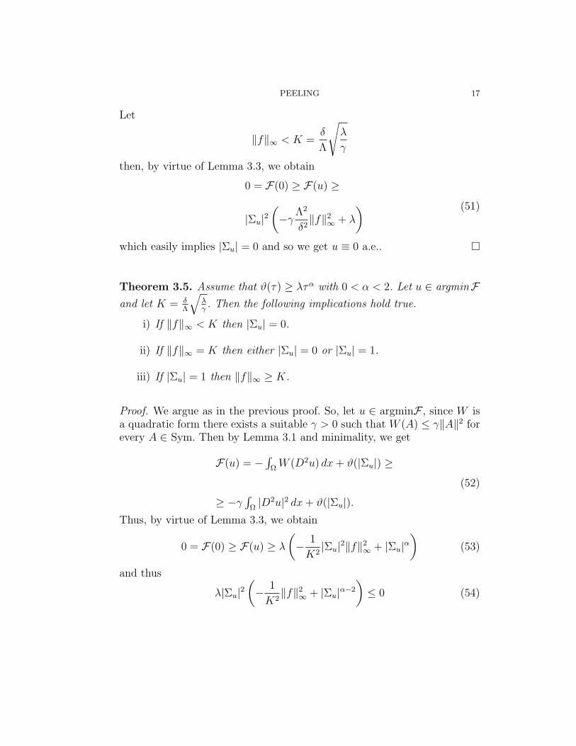
Let

‖f‖∞ < K =δ

Λ

√λ

γ

then, by virtue of Lemma 3.3, we obtain

0 = F(0) ≥ F(u) ≥

|Σu|2(−γΛ2

δ2‖f‖2

∞ + λ

) (51)

which easily implies |Σu| = 0 and so we get u ≡ 0 a.e..

Theorem 3.5. Assume that ϑ(τ) ≥ λτα with 0 < α < 2. Let u ∈ argminFand let K = δ

Λ

√λγ. Then the following implications hold true.

i) If ‖f‖∞ < K then |Σu| = 0.

ii) If ‖f‖∞ = K then either |Σu| = 0 or |Σu| = 1.

iii) If |Σu| = 1 then ‖f‖∞ ≥ K.

Proof. We argue as in the previous proof. So, let u ∈ argminF , since W isa quadratic form there exists a suitable γ > 0 such that W (A) ≤ γ‖A‖2 forevery A ∈ Sym. Then by Lemma 3.1 and minimality, we get

F(u) = −∫

ΩW (D2u) dx+ ϑ(|Σu|) ≥

≥ −γ∫

Ω|D2u|2 dx+ ϑ(|Σu|).

(52)

Thus, by virtue of Lemma 3.3, we obtain

0 = F(0) ≥ F(u) ≥ λ

(− 1

K2|Σu|2‖f‖2

∞ + |Σu|α)

(53)

and thus

λ|Σu|2(− 1

K2‖f‖2

∞ + |Σu|α−2

)≤ 0 (54)

18 PEELING

To prove the first assertion let us see that if |Σu| 6= 0, since 0 < α < 2and |Σu| ≤ 1, then (54) implies ‖f‖∞ ≥ K. The second assertion follows byconsidering that if ‖f‖∞ = K, then (54) becomes

λ|Σu|2(−1 + |Σu|α−2

)≤ 0,

from which we get the thesis. Finally, by substituting |Σu| = 1 in (54), weget

λ

(− 1

K2‖f‖2

∞ + 1

)≤ 0,

which proves the last statement.

We point out that the condition ‖f‖∞ = K defines a bifurcation pointin correspondence of which the material system exhibits a catastrophe likebehavior. At this value of the load, both the states of plate completelybonded and plate completely detached are admissible. Therefore, by con-sidering a monotone increasing variation of the load starting from the valueK, we can expect two possible scenarios. That is, if |Σu| = 0 the systemwill expend energy in deforming the plate and in breaking the adhesive,whereas if |Σu| = 1 the only further energy will be expended in the elasticdeformation of the plate.

Finally, let us notice that K = δΛ

√λγ

plays the role of a threshold on

the force f . Likewise the case of elastic beam studied in Section 2, where theanalogous parameter is denoted by fcr, K depends on the elastic stiffness ofthe plate through the ratio δ√

γ, on the stiffness of the adhesive layer through

√λ and on a geometric parameter Λ.

References

[1] L. Ambrosio, N. Fusco & D. Pallara,Functions of Bounded Variation and Free Dis-continuity Problems, Clarendon Press, Oxford, 2000.

[2] K.T. Andrews, L. Chapman, J.R. Fernandez, M. Fisackerly, L. Vanerian, T. Van-Houten, A membrane in adhesive contact, SIAM J. Appl. Math. (2003) 64, 152-169.

[3] J.L. Ericksen, Introduction to the Thermodynamics of solids, Chapman & Hall, 1991.[4] M. Fremond, Contact with adhesion, Chapter IV of Topics in Nonsmooth Mechanics,

Birkhauser Verlag (1988).[5] A. Ghatak, L. Mahadevan, J.Y. Chung, M.K. Chaudhury, V. Shenoy Peeling from

a biomimetically patterned thin elastic film, Proc. Royal Soc. London A (2004) 460,2725-2735.

[6] N. Israelachvili, Intramolecular and Surface Forces, Academic Press, New York(1992).

PEELING 19

[7] K.L. Johnson, Adhesion and friction between a smooth elastic spherical asperity anda smooth surface, Proc. Royal Soc. London A (1997) 453, 163-179.

[8] F. Maddalena & D. Percivale, Forthcoming.[9] V. G. Maz’ja, Sobolev Spaces, Springer-Verlag, 1985.

[10] X. Oyharcabal & T. Frisch, Peeling off an elastica from a smooth atractive substrate,Physical Review E 71, pp.036611-6 (2005).

[11] D. Percivale & F. Tomarelli, Smooth and creased equilibria for elastic-plastic platesand beams,Preprint.

[12] N. Pede, P. Podio-Guidugli, G. Tomassetti, Balancing the force that drives the peelingof an adhesive tape, Preprint.

[13] P. Podio-Guidugli, Peeling tapes, in Mechanics of Material Forces, ed. by P. Stein-mann and G. Maugin, Springer-Verlag (2005).

[14] P. Villaggio, Qualitative methods in elasticity, Noordhoff International Publishing,1977.

[15] Y. Wei & J.W. Hutchinson, Interface strenght, work of adhesion and plasticity inthe peel test,Int. Journ. of Fracture, 93, (1998), 315-333.

[16] Y.-P. Zhao, L.S. Wang & T.X. Yu, Mechanics of adhesion in MEMS – a review, J.Adhesion Sci. Technol., Vol. 17, No. 4, pp. 519-546 (2003).

Dipartimento di Matematica Politecnico di Bari, via Orabona 4, 70125Bari, Italy

Dipartimento di Ingegneria della Produzione Termoenergetica e Mod-elli Matematici, Universita di Genova, Piazzale Kennedy, Fiera del Mare,Padiglione D, 16129 Genova, Italy

E-mail address: maddalen@dm.uniba.it, percivale@diptem.unige.it