Poincare Analyticity and the Complete Variational Equations

D. Kaltcheva,∗ and A. J. Dragtb,†

a TRIUMF, 4004 Wesbrook Mall, Vancouver, B.C., Canada V6T 2A3kaltchev@triumf.ca

b Physics Department, University of Maryland, College Park, Maryland 20742, USAdragt@umd.edu

February 17, 2011

Abstract

According to a theorem of Poincare, the solutions to differential equations are analyticfunctions of (and therefore have Taylor expansions in) the initial conditions and variousparameters providing the right sides of the differential equations are analytic in the vari-ables, the time, and the parameters. We describe how these Taylor expansions may beobtained, to any desired order, by integration of what we call the complete variationalequations. As illustrated in a Duffing equation stroboscopic map example, these Taylor ex-pansions, truncated at an appropriate order thereby providing polynomial approximations,can well reproduce the behavior (including infinite period doubling cascades and strangeattractors) of the solutions of the underlying differential equations.

1 Introduction

In his prize-winning essay[1,2] and subsequent monumental work on celestial mechanics[3],Poincare established and exploited the fact that solutions to differential equations arefrequently analytic functions of the initial conditions and various parameters (should anyoccur). This result is often referred to as Poincare analyticity or Poincare’s theorem onanalyticity.

∗Corresponding author.†Work supported in part by U.S. Department of Energy Grant DE-FG02-96ER40949.

1

arX

iv:1

102.

3394

v1 [

mat

h-ph

] 1

6 Fe

b 20

11

Specifically, consider any set of m first-order differential equations of the form

za = fa(z1, · · · , zm; t;λ1, · · · , λn), a = 1, · · · ,m. (1.1)

Here t is the independent variable, the za are dependent variables, and the λb are possibleparameters. Let the quantities z0

a be initial conditions specified at some initial time t = t0,

za(t0) = z0a. (1.2)

Then, under mild conditions imposed on the functions fa that appear on the right side of(1.1) and thereby define the set of differential equations, there exists a unique solution

za(t) = ga(z01 , · · · , z0

m; t0, t;λ1, · · · , λn), a = 1,m (1.3)

of (1.1) with the property

za(t0) = ga(z01 , · · · , z0

m; t0, t0;λ1, · · · , λn) = z0a, a = 1,m. (1.4)

Now assume that the functions fa are analytic (within some domain) in the quantitiesza, the time t, and the parameters λb. Then, according to Poincare’s Theorem, the solutiongiven by (1.3) will be analytic (again within some domain) in the initial conditions z0

a, thetimes t0 and t, and the parameters λb.

Poincare established this result on a case-by-case basis as needed using Cauchy’s methodof majorants. It is now more commonly established in general using Picard iteration, andappears as background material in many standard texts on ordinary differential equations[4].

If the solution za(t) is analytic in the initial conditions z0a and the parameters λb, then

it is possible to expand it in the form of a Taylor series, with time-dependent coefficients, inthe variables z0

a and λb. The aim of this paper is to describe how these Taylor coefficientscan be found as solutions to what we will call the complete variational equations.

To aid further discussion, it is useful to also rephrase our goal in the context of maps.Suppose we rewrite the set of first-order differential equations (1.1) in the more compactvector form

z = f(z; t;λ). (1.5)

Then, again using vector notation, their solution can be written in the form

z(t) = g(z0; t0, t;λ). (1.6)

That is, the quantities z(t) at any time t are uniquely specified by the initial quantities z0

given at the initial time t0.We capitalize on this fact by introducing a slightly different notation. First, use ti

instead of t0 to denote the initial time. Similarly use zi to denote initial conditions bywriting

zi = z0 = z(ti). (1.7)

2

Next, let tf be some final time, and define final conditions zf by writing

zf = z(tf ). (1.8)

Then, with this notation, (1.6) can be rewritten in the form

zf = g(zi; ti, tf ;λ). (1.9)

We now view (1.9) as a map that sends the initial conditions zi to the final conditionszf . This map will be called the transfer map between the times ti and tf , and will bedenoted by the symbolM. What we have emphasized is that a set of first-order differentialequations of the form (1.5) can be integrated to produce a transfer map M. We expressthe fact that M sends zi to zf in symbols by writing

zf =Mzi, (1.10)

and illustrate this relation by the picture shown in Figure 1. We also note that M isalways invertible: Given zf , tf , and ti, we can always integrate (1.5) backward in timefrom the moment t = tf to the moment t = ti and thereby find the initial conditions zi.In the context of maps, our goal is to find a Taylor representation for M. If parametersare present, we may wish to have an expansion in some or all of them as well.

ZZ i f

M

Figure 1: The transfer map M sends the initial conditions zi to the final conditions zf .

The organization of this paper is as follows: Section 2 derives the complete variationalequations without and with dependence on some or all parameters. Sections 3 and 4describe their solution using forward and backward integration. As an example, Section 5treats the Duffing equation and describes the properties of an associated stroboscopic mapM. Section 6 sets up the complete variational equations for the Duffing equation, includingsome parameter dependence, and studies some of the properties of the map obtained bysolving these variational equations numerically. There we will witness the remarkable

3

fact that a truncated Taylor map approximation to M can reproduce the infinite period-doubling Feigenbaum cascade and associated strange attractor exhibited by the exact M.Section 7 describes how the variational equations can be solved numerically. A final sectionprovides a concluding summary.

2 Complete Variational Equations

This section derives the complete variational equations, first without parameter depen-dence, and then with parameter dependence.

2.1 Case of No or Ignored Parameter Dependence

Suppose the equations (1.1) do not depend on any parameters λb or we do not wish tomake expansions in them. We may then suppress their appearance to rewrite (1.1) in theform

za = fa(z, t), a = 1,m. (2.1)

Suppose that zd(t) is some given design solution to these equations, and we wish to studysolutions in the vicinity of this solution. That is, we wish to make expansions about thissolution. Introduce deviation variables ζa by writing

za = zda + ζa. (2.2)

Then the equations of motion (2.1) take the form

zda + ζa = fa(zd + ζ, t). (2.3)

In accord with our hypothesis of analyticity, assume that the right side of (2.3) is analyticabout zd. Then we may write the relation

fa(zd + ζ, t) = fa(zd, t) + ga(zd, t, ζ) (2.4)

where each ga has a Taylor expansion of the form

ga(zd, t, ζ) =∑r

gra(t)Gr(ζ). (2.5)

Here the Gr(ζ) are the various monomials in the m variables ζb labeled by an index r usingsome convenient labeling scheme, and the gra are (generally) time-dependent coefficientswhich we call forcing terms.1 By construction, all the monomials occurring in the rightside of (2.5) have degree one or greater. We note that the gra(t) are known once zd(t) isgiven.

1Here and in what follows the quantities ga are not to be confused with those appearing in (1.3).

4

By assumption, zd is a solution of (2.3) and therefore satisfies the relations

zda = fa(zd, t). (2.6)

It follows that the deviation variables satisfy the equations of motion

ζa = ga(zd, t, ζ) =∑r

gra(t)Gr(ζ). (2.7)

These equations are evidently generalizations of the usual first-degree (linear) variationalequations, and will be called the complete variational equations.

Consider the solution to the complete variational equations with initial conditions ζibspecified at some initial time ti. Following Poincare, we expect that this solution will bean analytic function of the initial conditions ζib. Also, since the right side of (2.7) vanisheswhen all ζb = 0 [all the monomials Gr in (2.7) have degree one or greater], ζ(t) = 0 is asolution to (2.7). It follows that the solution to the complete variational equations has aTaylor expansion of the form

ζa(t) =∑r

hra(t)Gr(ζi) (2.8)

where the hra(t) are functions to be determined, and again all the monomials Gr that occurhave degree one or greater. When the quantities hra(t) are evaluated at some final time tf ,(2.8) provides a representation of the transfer mapM about the design orbit in the Taylorform

ζfa = ζa(tf ) =∑r

hra(tf )Gr(ζi). (2.9)

2.2 Complete Variational Equations with Parameter Dependence

What can be done if we desire to have an expansion in parameters as well? Suppose thatthere are n such parameters, or that we wish to have expansions in n of them. The work ofthe previous section can be extended to handle this case by means of a simple trick: Viewthe n parameters as additional variables, and “augment” the set of differential equationsby additional differential equations that ensure these additional variables remain constant.

In detail, suppose we label the parameters so that those in which we wish to have anexpansion are λ1 · · ·λn. Introduce n additional variables zm+1, · · · z` where ` = m + n bymaking the replacements

λb → zm+b, b = 1, n. (2.10)

Next augment the equations (1.1) by n more of the form

za = 0, a = m+ 1, `. (2.11)

5

By this device we can rewrite the equations (1.1) in the form

za = fa(z, t), a = 1, ` (2.12)

with the understanding that

fa = fa(z; t;λrem), a = 1,m, (2.13)

where λrem denotes the other remaining parameters, if any, and

fa = 0, a = m+ 1, `. (2.14)

For the first m equations we impose, as before, the initial conditions

za(ti) = zia, a = 1,m. (2.15)

For the remaining equations we impose the initial conditions

za(ti) = λa−m, a = m+ 1, `. (2.16)

Note that the relations (2.14) then ensure the za for a > m retain these values for all t.To continue, let zd(t) be some design solution. Then, by construction, we have the

resultzda(t) = λda−m = λa−m, a = m+ 1, `. (2.17)

Again introduce deviation variables by writing

za = zda + ζa a = 1, `. (2.18)

Then the quantities ζa for a > m will describe deviations in the parameter values. More-over, because we have assumed analyticity in the parameters as well, relations of the forms(2.4) and (2.5) will continue to hold except that the Gr(ζ) are now the various monomialsin the ` variables ζb. Relations of the forms (2.6) and (2.7) will also hold with the provisos(2.13) and (2.14) and

gra(t) = 0, a = m+ 1, `. (2.19)

Therefore, we will only need to integrate the equations of the forms (2.6) and (2.7) fora ≤ m. Finally, relations of the form (2.9) will continue to hold for a ≤ m supplementedby the relations

ζfa = ζia, a = m+ 1, `. (2.20)

Since the Gr(ζi) now involve ` variables, the relations of the form (2.9) will provide an

expansion of the final quantities ζfa (for a ≤ m) in terms of the initial quantities ζia (fora ≤ m) and also the parameter deviations ζia with a = m+ 1, `.

6

3 Solution of Complete Variational Equations Using For-ward Integration

This section and the next describe two methods for the solution of the complete variationalequations. This section describes the method that employs integration forward in time,and is the conceptually simpler of the two methods.

3.1 Method of Forward Integration

To determine the functions hra, let us insert the expansion (2.8) into both sides of (2.7).With r′′ as a dummy index, the left side becomes the relation

ζa =∑r′′

hr′′

a (t)Gr′′(ζi). (3.1)

For the right side we find the intermediate result

∑r

gra(t)Gr(ζ) =∑r

gra(t) Gr

(∑r′

hr′

1 (t)Gr′(ζi), · · ·

∑r′

hr′

m(t)Gr′(ζi)

). (3.2)

However, since the Gr are monomials, there are relations of the form

Gr

(∑r′

hr′

1 (t)Gr′(ζi), · · ·

∑r′

hr′

m(t)Gr′(ζi)

)=∑r′′

U r′′r (hsn)Gr′′(ζ

i), (3.3)

and therefore the right side of (2.7) can be rewritten in the form∑r

gra(t)Gr(ζ) =∑r′′

∑r

gra(t)U r′′r (hsn)Gr′′(ζ

i). (3.4)

The notation U r′′r (hsn) is employed to indicate that these quantities might (at this stage of

the argument) depend on all the hsn with n ranging from 1 to m, and s ranging over allpossible values.

Now, in accord with (2.7), equate the right sides of (3.1) and (3.4) to obtain the relation∑r′′

hr′′

a (t)Gr′′(ζi) =

∑r′′

∑r

gra(t)U r′′r (hsn)Gr′′(ζ

i). (3.5)

Since the monomials Gr′′(ζi) are linearly independent, we must have the result

hr′′

a (t) =∑r

gra(t)U r′′r (hsn). (3.6)

7

We have found a set of differential equations that must be satisfied by the hra. Moreover,from (2.8) there is the relation

ζa(ti) =∑r

hra(ti)Gr(ζi) = ζia. (3.7)

Thus, all the functions hra(t) have a known value at the initial time ti, and indeed aremostly initially zero. When the equations (3.6) are integrated forward from t = ti to t = tf

to obtain the quantities hra(tf ), the result is the transfer mapM about the design orbit inthe Taylor form (2.9).

Let us now examine the structure of this set of differential equations. A key observationis that the functions U r′′

r (hsn) are universal. That is, as (3.3) indicates, they describe certaincombinatorial properties of monomials. They depend only on the dimensionm of the systemunder study, and are the same for all such systems. As (2.7) shows, what are peculiar toany given system are the forcing terms gra(t).

3.2 Application of Forward Integration to the Two-variable Case

To see what is going on in more detail, it is instructive to work out the first nontrivial case,that with m = 2. For two variables, all monomials in (ζ1, ζ2) are of the form (ζ1)j1(ζ2)j2 .Here, to simplify notation, we have dropped the superscript i. Table 1 below shows aconvenient way of labeling such monomials, and for this labeling we write

Gr(ζ) = (ζ1)j1(ζ2)j2 (3.8)

withj1 = j1(r) and j2 = j2(r). (3.9)

Table 1: A labeling scheme for monomials in two variables.

r j1 j2 D

1 1 0 12 0 1 13 2 0 24 1 1 25 0 2 26 3 0 37 2 1 38 1 2 39 0 3 3

8

Thus, for example,G1 = ζ1, (3.10)

G2 = ζ2, (3.11)

G3 = ζ21 , (3.12)

G4 = ζ1ζ2, (3.13)

G5 = ζ22 , etc. (3.14)

For more detail about monomial labeling schemes, see Section 7.Let us now compute the first few U r′′

r (hsn). From (3.3) and (3.10) we find the relation

G1

(∑r′

hr′

1 Gr′(ζ),∑r′

hr′

2 Gr′(ζ)

)=∑r′

hr′

1 Gr′(ζ) =∑r′′

U r′′1 Gr′′(ζ). (3.15)

It follows that there is the resultU r′′

1 = hr′′

1 . (3.16)

Similarly, from (3.3) and (3.11), we find the result

U r′′2 = hr

′′2 . (3.17)

From (3.3) and (3.12) we find the relation

G3

(∑r′

hr′

1 Gr′(ζ),∑r′

hr′

2 Gr′(ζ)

)=

(∑r′

hr′

1 Gr′(ζ)

)2

=∑s,t

hs1ht1Gs(ζ)Gt(ζ) =

∑r′′

U r′′3 Gr′′(ζ). (3.18)

Use of (3.18) and inspection of (3.10) through (3.14) yields the results

U13 = 0, (3.19)

U23 = 0, (3.20)

U33 = (h1

1)2, (3.21)

U43 = 2h1

1h21, (3.22)

U53 = (h2

1)2. (3.23)

From (3.3) and (3.13) we find the relation

G4

(∑r′

hr′

1 Gr′(ζ),∑r′

hr′

2 Gr′(ζ)

)=

(∑r′

hr′

1 Gr′(ζ)

)(∑r′

hr′

2 Gr′(ζ)

)=

∑s,t

hs1ht2Gs(ζ)Gt(ζ) =

∑r′′

U r′′4 Gr′′(ζ). (3.24)

9

It follows that there are the resultsU1

4 = 0, (3.25)

U24 = 0, (3.26)

U34 = h1

1h12, (3.27)

U44 = h1

1h22 + h2

1h12, (3.28)

U54 = h2

1h22. (3.29)

Finally, from (3.3) and (3.14), we find the results

U15 = 0, (3.30)

U25 = 0, (3.31)

U35 = (h1

2)2, (3.32)

U45 = 2h1

2h22, (3.33)

U55 = (h2

2)2. (3.34)

Two features now become apparent. As in Table 1, let D(r) be the degree of themonomial with label r. Then, from the examples worked out, and quite generally from(3.3), we see that there is the relation

U r′′r = 0 when D(r) > D(r′′). (3.35)

It follows that the sum on the right side of (3.6) always terminates. Second, for thearguments hsn possibly appearing in U r′′

r (hsn), we see that there is the relation

D(s) ≤ D(r′′). (3.36)

It follows, again see (3.6), that the right side of the differential equation for any hr′′

a involvesonly the hsn for which (3.36) holds. Therefore, to determine the coefficients hra(tf ) of theTaylor expansion (2.9) through terms of some degree D, it is only necessary to integrate afinite number of equations, and the right sides of these equations involve only the coefficientsfor this degree and lower.

For example, to continue our discussion of the case of two variables, the equations (3.6)take the explicit form

h11(t) =

2∑r=1

gr1(t)U1r = g1

1(t)h11(t) + g2

1(t)h12(t), (3.37)

h12(t) =

2∑r=1

gr2(t)U1r = g1

2(t)h11(t) + g2

2(t)h12(t), (3.38)

10

h21(t) =

2∑r=1

gr1(t)U2r = g1

1(t)h21(t) + g2

1(t)h22(t), (3.39)

h22(t) =

2∑r=1

gr2(t)U2r = g1

2(t)h21(t) + g2

2(t)h22(t), (3.40)

h31(t) =

5∑r=1

gr1(t)U3r

= g11(t)h3

1(t) + g21(t)h3

2(t) + g31(t)[h1

1(t)]2

+g41(t)h1

1(t)h12(t) + g5

1(t)[h12(t)]2, (3.41)

h32(t) =

5∑r=1

gr2(t)U3r

= g12(t)h3

1(t) + g22(t)h3

2(t) + g32(t)[h1

1(t)]2

+g42(t)h1

1(t)h12(t) + g5

2(t)[h12(t)]2, (3.42)

h41(t) =

5∑r=1

gr1(t)U4r

= g11(t)h4

1(t) + g21(t)h4

2(t) + 2g31(t)h1

1(t)h21(t)

+g41(t)[h1

1(t)h22(t) + h2

1(t)h12(t)] + 2g5

1(t)h12(t)h2

2(t), (3.43)

h42(t) =

5∑r=1

gr2(t)U4r

= g12(t)h4

1(t) + g22(t)h4

2(t) + 2g32(t)h1

1(t)h21(t)

+g42(t)[h1

1(t)h22(t) + h2

1(t)h12(t)] + 2g5

2(t)h12(t)h2

2(t), (3.44)

h51(t) =

5∑r=1

gr1(t)U5r

= g11(t)h5

1(t) + g21(t)h5

2(t) + g31(t)[h2

1(t)]2

+g41(t)h2

1(t)h22(t) + g5

1(t)[h22(t)]2, (3.45)

h52(t) =

5∑r=1

gr2(t)U5r

= g12(t)h5

1(t) + g22(t)h5

2(t) + g32(t)[h2

1(t)]2

+g42(t)h2

1(t)h22(t) + g5

2(t)[h22(t)]2, etc. (3.46)

11

And, from (3.7), we have the initial conditions

hra(ti) = δra. (3.47)

We see that if we desire only the degree one terms in the expansion (2.8), then it isonly necessary to integrate the equations (3.37) through (3.40) with the initial conditions(3.47). A moment’s reflection shows that so doing amounts to integrating the first-degreevariational equations. We also observe that if we desire only the degree one and degreetwo terms in the expansion (2.8), then it is only necessary to integrate the equations (3.37)through (3.46) with the initial conditions (3.47), etc.

4 Solution of Complete Variational Equations Using Back-ward Integration

There is another method of determining the hra that is surprising, ingenious, and in someways superior to that just described. It involves integrating backward in time[5].

4.1 Method of Backward Integration

Let us rewrite (2.9) in the slightly more explicit form

ζfa =∑r

hra(ti, tf )Gr(ζi) (4.1)

to indicate that there are two times involved, ti and tf . From this perspective, (3.6) is aset of differential equations for the quantities (∂/∂t)hra(ti, t) that is to be integrated andevaluated at t = tf . An alternate procedure is to seek a set of differential equations for thequantities (∂/∂t)hra(t, tf ) that is to be integrated and evaluated at t = ti.

As a first step in considering this alternative, rewrite (4.1) in the form

ζfa =∑r

hra(t, tf )Gr(ζ(t)). (4.2)

Now reason as follows: If t is varied and at the same time the quantities ζ(t) are varied(evolve) so as to remain on the solution to (2.7) having final conditions ζf , then thequantities ζf must remain unchanged. Consequently, there is the differential equationresult

0 = dζfa /dt =∑r

[(∂/∂t)ha(t, tf )]Gr(ζ(t)) +∑r

hra(t, tf )(d/dt)Gr(ζ(t)). (4.3)

Let us introduce the notation hra(t, tf ) for (∂/∂t)hra(t, tf ) so that the first term on theright side of (4.3) can be rewritten in the form∑

r

[(∂/∂t)hra(t, tf )]Gr(ζ) =∑r

hraGr(ζ). (4.4)

12

Next, begin working on the second term on the right side of (4.3) by replacing the sum-mation index r by the dummy index r′,∑

r

hra(t, tf )(d/dt)Gr(ζ(t)) =∑r′

hr′

a (t, tf )(d/dt)Gr′(ζ(t)). (4.5)

Now carry out the indicated differentiation using the chain rule and the relation (2.7) whichdescribes how the quantities ζ vary along a solution,

(d/dt)Gr′(ζ(t)) =∑b

(∂Gr′/∂ζb)(dζb/dt) =∑br′′

(∂Gr′/∂ζb)gr′′b (t)Gr′′(ζ(t)). (4.6)

Watch closely: Since the Gr are simply standard monomials in the ζ, there must berelations of the form

[(∂/∂ζb)Gr′(ζ)]Gr′′(ζ) =∑r

Crbr′r′′Gr(ζ) (4.7)

where the Crbr′r′′ are universal constant coefficients that describe certain combinatorial

properties of monomials. As a result, the second term on the right side of (4.3) can bewritten in the form∑

r′

hr′

a (t, tf )(d/dt)Gr′(ζ(t)) =∑r

Gr(ζ)∑br′r′′

Crbr′r′′g

r′′b (t)hr

′a (t, tf ). (4.8)

Since the monomials Gr are linearly independent, the relations (4.3) through (4.8) implythe result

hra(t, tf ) = −∑br′r′′

Crbr′r′′g

r′′b (t)hr

′a (t, tf ). (4.9)

This result is a set of differential equations for the hra that are to be integrated fromt = tf back to t = ti. Also, evaluating (4.2) for t = tf gives the results

ζfa =∑r

hra(tf , tf )Gr(ζfa ), (4.10)

from which it follows that (with the usual polynomial labeling) the hra satisfy the finalconditions

hra(tf , tf ) = δra. (4.11)

Therefore the solution to (4.9) is uniquely defined. Finally, it is evident from the definition(4.7) that the coefficients Cr

br′r′′ satisfy the relation

Crbr′r′′ = 0 unless [D(r′)− 1] +D(r′′) = D(r). (4.12)

Therefore, since D(r′′) ≥ 1 in (4.9), it follows from (4.12) that the only hr′

a that occur onthe right side of (4.9) are those that satisfy

D(r′) ≤ D(r). (4.13)

13

Similarly, the only gr′′

b that occur are those that satisfy

D(r′′) ≤ D(r). (4.14)

Therefore, as before, to determine the coefficients hra of the Taylor expansion (2.9) throughterms of some degree D, it is only necessary to integrate a finite number of equations, andthe right sides of these equations involve only the coefficients for this degree and lower.

Comparison of the differential equation sets (3.6) and (4.9) shows that the latter hasthe remarkable property of being linear in the unknown quantities hra. This feature meansthat the evaluation of the right side of (4.9) involves only the retrieval of certain universalconstants Cr

br′r′′ and straight-forward multiplication and addition. By contrast, the use of(3.6) requires evaluation of the fairly complicated nonlinear functions U r′′

r (hsn). Finally, itis easier to insure that a numerical integration procedure is working properly for a set oflinear differential equations than it is for a nonlinear set.

The only complication in the use of (4.9) is that the equations must be integratedbackwards in t. Correspondingly the equations (2.6) for the design solution must also beintegrated backwards since they supply the required quantities gra through use of (2.4) and(2.5). This is no problem if the final quantities zd(tfin) are known. However if only theinitial quantities zd(tin) are known, then the equations (2.6) for zd must first be integratedforward in time to find the final quantities zd(tfin).

4.2 The Two-variable Case Revisited

For clarity, let us also apply this second method to the two-variable case. Table 2 showsthe nonzero values of Cr

br′r′′ for r ∈ [1, 5] obtained using (3.10) through (3.14) and (4.7).Note that the rules (4.12) hold. Use of this Table shows that in the two-variable case theequations (4.9) take the form

h11(t, tf ) = − g1

1(t)h11(t, tf )− g1

2(t)h21(t, tf ), (4.15)

h12(t, tf ) = − g1

1(t)h12(t, tf )− g1

2(t)h22(t, tf ), (4.16)

h21(t, tf ) = − g2

1(t)h11(t, tf )− g2

2(t)h21(t, tf ), (4.17)

h22(t, tf ) = − g2

1(t)h12(t, tf )− g2

2(t)h22(t, tf ), (4.18)

h31(t, tf ) = − 2g1

1(t)h31(t, tf )− g3

1(t)h11(t, tf )− g1

2(t)h41(t, tf )− g3

2(t)h21(t, tf ), (4.19)

h32(t, tf ) = − 2g1

1(t)h32(t, tf )− g3

1(t)h12(t, tf )− g1

2(t)h42(t, tf )− g3

2(t)h22(t, tf ), (4.20)

h41(t, tf ) = − g1

1(t)h41(t, tf )− 2g2

1(t)h31(t, tf )− g4

1(t)h11(t, tf )

−2g12(t)h5

1(t, tf )− g22(t)h4

1(t, tf )− g42(t)h2

1(t, tf ), (4.21)

14

h42(t, tf ) = − g1

1(t)h42(t, tf )− 2g2

1(t)h32(t, tf )− g4

1(t)h12(t, tf )

−2g12(t)h5

2(t, tf )− g22(t)h4

2(t, tf )− g42(t)h2

2(t, tf ), (4.22)

h51(t, tf ) = − g2

1(t)h41(t, tf )− g5

1(t)h11(t, tf )− 2g2

2(t)h51(t, tf )− g5

2(t)h21(t, tf ), (4.23)

h52(t, tf ) = − g2

1(t)h42(t, tf )− g5

1(t)h12(t, tf )− 2g2

2(t)h52(t, tf )− g5

2(t)h22(t, tf ), etc. (4.24)

As advertised, the right sides of (4.15) through (4.24) are indeed simpler than those of(3.37) through (3.46).

Table 2: Nonzero values of Crbr′r′′ for r ∈ [1, 5] in the two-variable case.

r b r′ r′′ C

1 1 1 1 11 2 2 1 12 1 1 2 12 2 2 2 13 1 1 3 13 1 3 1 23 2 2 3 13 2 4 1 14 1 1 4 14 1 3 2 24 1 4 1 14 2 2 4 14 2 4 2 14 2 5 1 25 1 1 5 15 1 4 2 15 2 2 5 15 2 5 2 1

5 Duffing Equation Example

5.1 Introduction

As an example application, this section studies some aspects of the Duffing equation.The behavior of the driven Duffing oscillator, like that of generic nonlinear systems, isenormously complicated. Consequently, we will be able to only touch on some of thehighlights of this fascinating problem.

15

Duffing’s equation describes the behavior of a periodically driven damped nonlinearoscillator governed by the equation of motion

x+ ax+ bx+ cx3 = d cos(Ωt+ ψ). (5.1)

Here ψ is an arbitrary phase factor that is often set to zero. For our purposes it is moreconvenient to set

ψ = π/2. (5.2)

Evidently any particular choice of ψ simply results in a shift of the origin in time, and thisshift has no physical consequence since the left side of (5.1) is independent of time.

We assume b, c > 0, which is the case of a positive hard spring restoring force.2 Wemake these assumptions because we want the Duffing oscillator to behave like an ordinaryharmonic oscillator when the amplitude is small, and we want the motion to be boundedaway from infinity when the amplitude is large. Then, by a suitable choice of time andlength scales that introduces new variables q and τ , the equation of motion can be broughtto the form

q + 2βq + q + q3 = −ε sinωτ, (5.3)

where now a dot denotes d/dτ and we have made use of (5.2). In this form it is evidentthat there are 3 free parameters: β, ε, and ω.

5.2 Stroboscopic Map

While the Duffing equation is nonlinear, it does have the simplifying feature that thedriving force is periodic with period

T = 2π/ω. (5.4)

Let us convert (5.3) into a pair of first-order equations by making the definition

p = q, (5.5)

with the resultq = p,

p = −2βp− q − q3 − ε sinωτ. (5.6)

Let q0, p0 denote initial conditions at τ = 0, and let q1, p1 be the final conditions resultingfrom integrating the pair (5.6) one full period to the time τ = T . LetM denote the transfermap that relates q1, p1 to q0, p0. Then, using the notation z = (q, p), we may write

z1 =Mz0. (5.7)

2Other authors consider other cases, particularly the ‘double well’ case b < 0 and c > 0.

16

Suppose we now integrate for a second full period to find q2, p2. Since the right side of(5.6) is periodic, the rules for integrating from τ = T to τ = 2T are the same as the rulesfor integrating from τ = 0 to τ = T . Therefore we may write

z2 =Mz1 =M2z0, (5.8)

and in generalzn+1 =Mzn =Mn+1z0. (5.9)

We may regard the quantities zn as the result of viewing the motion in the light providedby a stroboscope that flashes at the times3

τn = nT. (5.10)

Because of the periodicity of the right side of the equations of motion, the rule for sendingzn to zn+1 over the intervals between successive flashes is always the same, namelyM. Forthese reasons M is called a stroboscopic map. Despite the explicit time dependence in theequations of motion, because of periodicity we have been able to describe the long-termmotion by the repeated application of a single fixed map.

5.3 Feigenbaum Diagram Overview

One way to study a map and analyze its properties, in this case the Duffing stroboscopicmap, is to find its fixed points. When these fixed points are found, one can then display howthey appear, move, and vanish as various parameters are varied. Such a display is oftencalled a Feigenbaum diagram. This subsection will present selected Feigenbaum diagrams,including the infinite period doubling cascade and its associated strange attractor, forthe stroboscopic map obtained by high-accuracy numerical integration of the equations ofmotion (5.6). They will be made by observing the behavior of fixed points as the drivingfrequency ω is varied. For simplicity, the damping parameter will be held constant at thevalue β = 0.10. Various sample values will be used for the driving strength ε.4

Let us begin with the case of small driving strength. When the driving strength issmall, we know from energy considerations that the steady-state response will be small,and therefore the behavior of the steady-state solution will be much like that of the drivendamped linear harmonic oscillator. That is, for small amplitude motion, the q3 term in (5.3)will be negligible compared to the other terms. We also know that, because of damping,there will be only one steady-state solution, and therefore M has only one fixed point zf

such thatMzf = zf . (5.11)

3Note that, with the choice (5.2) for ψ, the driving term described by the right side of (5.3) vanishes atthe stroboscopic times τn.

4Of course, one can also make Feigenbaum diagrams in which some other parameter, say ε, is variedwhile the others, including ω, are held fixed.

17

Finally, again because of damping, we know that this fixed point is stable. That is, if Mis applied repeatedly to a point near zf , the result is a sequence of points that approachever closer to zf . For this reason a stable fixed point is also called an attractor.

5.3.1 A Simple Feigenbaum Diagram

Figure 2 shows the values of qf (ω) and for the case ε = 0.150, and Figure 3 shows pf (ω). Inthe figures the phase-space axes are labeled as q∞ and p∞ to indicate that what are beingdisplayed are steady-state values reached after a large number of applications of M. Asanticipated, we observe from Figures 2 and 3 that the response is much like the resonanceresponse of the driven damped linear harmonic oscillator.5 Note that the coefficient of qin (5.12) is 1, and therefore at small amplitudes, where q3 can be neglected, the Duffingoscillator described by (5.3) has a natural frequency near 1. Correspondingly, Figure 2displays a large response when the driving frequency has the value ω ' 1. Observe,however, that the response, while similar, is not exactly like that of the driven dampedlinear harmonic oscillator. For example, the resonance peak at ω ' 1 is slightly tipped tothe right, and there is also a small peak for ω ' 1/3.

Our strategy for further exploration will be to increase the value of the driving strengthε, all the while observing the stroboscopic Duffing map Feigenbaum diagram as a functionof ω. We hasten to add the disclaimer that the driven Duffing oscillator displays anenormously rich behavior that varies widely with the parameter values β, ε, ω, and weshall be able to give a brief summary of some of it. Also, for brevity, we shall generallyonly display qf (ω).

5.3.2 Saddle-Node (Blue-Sky) Bifurcations

Figure 4 shows the q Feigenbaum diagram for the case of somewhat larger driving strength,ε = 1.50. For this driving strength the resonance peak, which previously occurred at ω ' 1,has shifted to a higher frequency and taken on a more complicated structure. There arenow also noticeable resonances at lower frequencies, with the most prominent one being atω ' 1/2.

Examination of Figure 4 shows that for ω ≤ 1.5 there is a single stable fixed pointwhose trail is shown in black. Then, as ω is increased, a pair of fixed points is born atω ' 1.8.6 One of them is stable. The other, whose trail as ω is varied is shown in red, isunstable. That is, if M is applied repeatedly to a point near this fixed point, the result isa sequence of points that move ever farther away from the fixed point. For this reason anunstable fixed point is also called a repellor.

5It was the desire for q∞ to exhibit a resonance-like peak as a function of ω that dictated the choice(5.2) for ψ.

6Actually, in the analytic spirit of Poincare, these fixed points also exist for smaller values of ω, but arethen complex. They first become purely real, and therefore physically apparent, when ω ' 1.8.

18

0

0.1

0.2

0.3

0.4

0.5

0.6

0.7

0 0.5 1 1.5 2 2.5

q∞

ω

Figure 2: Feigenbaum diagram showing limiting values q∞ as a function of ω (when β = 0.1and ε = .15) for the stroboscopic Duffing map.

19

-0.4

-0.3

-0.2

-0.1

0

0.1

0.2

0.3

0.4

0 0.5 1 1.5 2 2.5

p∞

ω

Figure 3: Feigenbaum diagram showing limiting values p∞ as a function of ω (when β = 0.1and ε = .15) for the stroboscopic Duffing map.

This appearance of two fixed points out of nowhere is called a saddle-node bifurcationor a blue-sky bifurcation, and the associated Fiegenbaum diagram is then sometimes calleda bifurcation diagram.7 The original stable fixed point persists as ω is further increased sothat over some ω range there are 3 fixed points. Then, as ω is further increased, the originalfixed point and the unstable fixed point move until they meet and annihilate when ω ' 2.6.8

This disappearance is called an inverse saddle-node or inverse blue-sky bifurcation. Finally,for still larger ω values there is again only one fixed point, and it is stable.

The appearance and disappearance of stable-unstable fixed-point pairs, as ω is varied,has a striking dynamical consequence. Suppose, for example in the case of Figure 4, thatthe driving frequency ω is below the value ω ' 1.8 where the saddle-node bifurcationoccurs. Then there is only one fixed point, and it is attracting. Now suppose ω is slowlyincreased. Then, since the fixed-point solution is attracting, the solution for the slowlyincreasing ω case will remain near this solution. See the upper black trail in Figure 4. This“tracking” will continue until ω reaches the value ω ' 2.6 where the inverse saddle-nodebifurcation occurs. At this value the fixed point being followed disappears. Consequently,since the one remaining fixed point is also an attractor, the solution evolves very quicklyto that of the remaining fixed point. It happens that the oscillation amplitude associated

7Strictly speaking, a Feigenbaum diagram displays only the trails of stable fixed points while a bifurcationdiagram displays the trails of all fixed points.

8Actually, they are not destroyed, but instead become complex and therefore disappear from view.

20

q∞

ω

0.5 1 1.5 2 2.5 3 3.5

3

0.5

0

1

1.5

2

2.5

Figure 4: Feigenbaum/bifurcation diagram showing limiting values q∞ as a function of ω(when β = 0.1 and ε = 1.5) for the stroboscopic Duffing map. Trails of the stable fixedpoints are shown in black. Also shown, in red, is the trail of the unstable fixed point.Finally, jumps in the steady-state amplitude are illustrated by vertical dashed lines atω ' 1.8 and ω ' 2.6.

21

with this fixed point is much smaller, and therefore there appears to be a sudden jumpin oscillation amplitude to a smaller value. Now suppose ω is slowly decreased from avalue above the value ω ' 2.6 where the inverse saddle-node bifurcation occurs. Thenthe solution will remain near that of the fixed point lying on the bottom black trail inFigure 4. This tracking will continue until ω reaches the value ω ' 1.8 where the fixedpoint being followed disappears. Again, since the remaining fixed point is attracting, thesolution will now evolve to that of the remaining fixed point. The result is a jump toa larger oscillation amplitude. Evidently the steady-state oscillation amplitude exhibitshysteresis as ω is slowly varied back and forth over an interval that begins below the valuewhere the first saddle-node bifurcation occurs and ends at a value above that where theinverse saddle-node bifurcation occurs.

5.3.3 Pitchfork Bifurcations

Let us continue to increase ε. Figure 5 shows that a qualitatively new feature appearswhen ε is near 2.2: a bubble is formed between the major resonant peak (the one thathas saddle-node bifurcated) and the subresonant peak immediately to its left. To explorethe nature of this bubble, let us make ε still larger, which, we anticipate, will result inthe bubble becoming larger. Figure 6 shows the Feigenbaum diagram in the case ε = 5.5.Now the major resonant peak and the subresonant peak have moved to larger ω values.Correspondingly, the bubble between them has also moved to larger ω values. Moreover,it is larger, yet another smaller bubble has formed, and the subresonant peak betweenthem has also undergone a saddle-node bifurcation. For future use, we will call the majorresonant peak the first or leading saddle-node bifurcation, and we will call the subresonantpeak between the two bubbles the second saddle-node bifurcation, etc. Also, we will callthe bubble just to the left of the first saddle-node bifurcation the first or leading bubble,and the next bubble will be called the second bubble, etc.

We also note that three short trails have appeared in Figure 6 just to the right ofω = 4. They correspond to a period-three bifurcation followed shortly thereafter by aninverse bifurcation. Actually, much closer examination shows that there are six trailsconsisting of three closely-spaced pairs. Each pair comprises a stable and an unstable fixedpoint of the map M3. They are not fixed points of M itself, but rather are sent into eachother in cyclic fashion under the action of M.

Figure 7 shows the larger (leading) bubble in Figure 6 in more detail and with theaddition of red lines indicating the trails of unstable fixed points. It reveals that the bubbledescribes the simultaneous bifurcation of a single fixed point into three fixed points. Twoof these fixed points are stable and the third, whose q coordinate as a function of ω areshown as a red line, is unstable. What happens is that, as ω is increased, a single stablefixed point becomes a triplet of fixed points, two of which are stable and one of which isunstable. This is called a pitchfork bifurcation. Then, as ω is further increased, these threefixed points again merge, in an inverse pitchfork bifurcation, to form what is again a single

22

-0.5

0

0.5

1

1.5

2

2.5

3

3.5

4

0 0.5 1 1.5 2 2.5 3 3.5

q∞

ω

Figure 5: Feigenbaum diagram showing limiting values q∞ as a function of ω (when β = 0.1and ε = 2.2) for the stroboscopic Duffing map. It displays that a bubble has now formedat ω ≈ .8.

23

-1

0

1

2

3

4

5

6

0 1 2 3 4 5 6

q∞

ω

Figure 6: Feigenbaum diagram showing limiting values q∞ as a function of ω (when β = 0.1and ε = 5.5) for the stroboscopic Duffing map. The first bubble has grown, a second smallerbubble has formed to its left, and the sub-resonant peak between them has saddle-nodebifurcated to become the second saddle-node bifurcation.

24

stable fixed point.

-1

-0.5

0

0.5

1

1.5

2

0.6 0.8 1 1.2 1.4

q∞

ω

Figure 7: An enlargement of Figure 6 with the addition of red lines indicating the trails ofunstable fixed points.

25

5.3.4 A Plethora of Bifurcations and Period Doubling Cascades

We end our study of the Duffing equation by increasing ε from its earlier value ε = 5.5 tomuch larger values. First we will set ε = 22.125. Based on our experience so far, we mightanticipate that the Feigenbaum diagram would become much more complicated. That isindeed the case. Figure 8 displays q∞ when β = 0.1 and ε = 22.125, as a function of ω, forthe range ω ∈ (0, 12). Evidently the behavior of the attractors for the stroboscopic Duffingmap, which is what is shown in Figure 8, is extremely complicated. There are now a greatmany fixed points both of M itself and various powers of M.

Of particular interest to us are the two areas around ω = .8 and ω = 1.25. Theycontain what has become of the first two bubbles in Figure 7, and are shown in greatermagnification in Figure 9. What has happened is that bubbles have formed within bubbles,and bubbles have formed within these bubbles, etc. to form a cascade. However, theseinterior bubbles are not the result of pitchfork bifurcations, but rather the result of period-doubling bifurcations. For example, the bifurcation that creates the first bubble at ω ' 1.2is a pitchfork bifurcation. But the successive bifurcations within the bubble are period-doubling bifurcations. In a period-doubling bifurcation a fixed point that is initially stablebecomes unstable as ω is increased. When this happens, simultaneously two stable fixedpoints of M2 are born. They are not fixed points of M itself, but rather are sent intoeach other under the action of M. Hence the name “period doubling”. The map M mustbe applied twice to send such a fixed point back into itself. In the next period doubling,fixed points of M4 are born, etc. However we note that, as ω increases, the sequence ofperiod-doubling bifurcations only occurs a finite number of times and then undoes itself.

Remarkably, when ε is just somewhat larger, infinite sequences of period doublingcascades can occur. Figure 10 shows what happens when ε = 25.

5.3.5 More Detailed View of Infinite Period Doubling Cascades

To display the infinite period doubling cascades in more detail, Figure 11 shows an en-largement of part of Figure 10. And Figures 12 and 13 show successive enlargements ofparts of the first bubble in Figure 10. From Figure 11 we see that the first bubble forms asa result of a pitchfork bifurcation just to the right of ω = 1.2, and from Figures 12 and 13we see that the first period doubling bifurcation occurs in the vicinity of ω = 1.268. FromFigure 13 it is evident that successive period-doublings occur an infinite number of timesto ultimately produce a chaotic region when ω exceeds ω ' 1.29.

5.3.6 Strange Attractor

As evidence that the behavior in this region is chaotic, Figures 14 and 15 show portionsof the full phase space, the q, p plane, when ω = 1.2902. Note the evidence for fractalstructure. The points appear to lie on a strange attractor.

26

-4-2 0 2 4 6 8

10

12

2 4

6 8

10

12

ω

q∞

Figure 8: Feigenbaum diagram showing limiting values q∞ as a function of ω (when β = 0.1and ε = 22.125) for the stroboscopic Duffing map.

27

-2

-1.5

-1

-0.5

0

0.5

1

1.5

2

2.5

0.6 0.8 1 1.2 1.4 1.6

ω

q∞

Figure 9: Enlarged portion of the Feigenbaum diagram of Figure 8 displaying limitingvalues q∞ as a function of ω (when β = 0.1 and ε = 22.125) for the stroboscopic Duffingmap. It shows part of the first bubble at the far right, the second bubble, and part of athird bubble at the far left. Examine the first and second bubbles. Each initially consistsof two stable period-one fixed points. Each also contains the beginnings of period-doublingcascades. These cascades do not complete, but rather remerge to again result in a pair ofstable period-one fixed points. There are also many higher-period fixed points and theirassociated cascades.

28

-4-2 0 2 4 6 8

10

12

14

0 2

4 6

8 1

0 1

2

ω

q∞

Figure 10: Feigenbaum diagram showing limiting values q∞ as a function of ω (whenβ = 0.1 and ε = 25) for the stroboscopic Duffing map.

29

-3

-2

-1

0

1

2

3

0.6 0.8 1 1.2 1.4 1.6 1.8 2 2.2

ω

q∞

Figure 11: Enlargement of a portion Figure 10 showing the first, second, and third bubbles.The period-doubling cascades in each of the first and second bubbles complete. Then theyundo themselves as ω is further increased. There is no period doubling in the third bubblewhen ε = 25.

30

-1.5

-1

-0.5

0

0.5

1

1.5

2

2.5

1.26 1.265 1.27 1.275 1.28 1.285 1.29 1.295

ω

q∞

Figure 12: Detail of part of the first bubble in Figure 11 showing upper and lower infiniteperiod-doubling cascades. Part of the trail of the stable fixed point associated with thesecond saddle-node bifurcation accidentally appears to overlay the upper period doublingbifurcation. Finally, there are numerous cascades and remergings associated with higher-period fixed points.

31

0.7

0.8

0.9

1

1.1

1.2

1.3

1.4

1.5

1.6

1.26 1.265 1.27 1.275 1.28 1.285 1.29

ω

q∞

Figure 13: Detail of part of the upper cascade in Figure 12 showing an infinite period-doubling cascade, followed by chaos, for what was initially a stable period-one fixed point.

32

1.75

1.8

1.85

1.9

1.95

2

2.05

2.1

2.15

0.7 0.8 0.9 1 1.1 1.2 1.3 1.4 1.5 1.6

p∞

q∞

Figure 14: Limiting values of q∞, p∞ for the stroboscopic Duffing map when ω = 1.2902(and β = .1 and ε = 25). They appear to lie on a strange attractor.

33

2

2.005

2.01

2.015

2.02

2.025

2.03

1.49 1.495 1.5 1.505 1.51 1.515 1.52 1.525 1.53

q∞

p∞

Figure 15: Enlargement of boxed portion of Figure 14 illustrating the beginning of self-similar fractal structure.

34

6 Polynomial Approximation to Duffing Stroboscopic Map

In this section we will find the complete variational equations for the Duffing equationincluding dependence on the parameter ω. The two remaining parameters, β and ε, willremain fixed. We will then study the properties of the resulting polynomial approximationto the Duffing stroboscopic map obtained by truncating its Taylor expansion.

6.1 Complete Variational Equations with Selected Parameter Depen-dence

To formulate the complete variational equations we could proceed as in Section 2.2 bysetting ω = z3 and z3 = ωd + ζ3. So doing would require expanding the function sin(ωτ) =sin[(ωd + ζ3)τ ] as a power series in ζ3. Such an expansion is, of course, possible, but itleads to variational equations with a large number of forcing terms gra since the expansionof sin[(ωd + ζ3)τ ] contains an infinite number of terms.

In the case of Duffing’s equation this complication can be avoided by a further changeof variables. Recall that the first change of variables brought the Duffing equation to theform (5.3), which we now slightly rewrite as

q′′ + 2βq′ + q + q3 = −ε sinωτ (6.1)

where d/dτ is now denoted by a prime. Next make the further change of variables

q = ωQ, (6.2)

ω = 1/σ, (6.3)

ωτ = t. (6.4)

When this is done, there are the relations

q′ = ω2Q (6.5)

andq′′ = ω3Q (6.6)

where now a dot denotes d/dt. [Note that the variable t here is different from that in (5.1).]Correspondingly, Duffing’s equation takes the form

Q+ 2βσQ+ σ2Q+Q3 = −εσ3 sin t. (6.7)

This equation can be converted to a first-order set of the form (2.1) by writing

Q = z1 (6.8)

35

andQ = z2. (6.9)

Following the method of Section 2.2, we augment the first-order equation set associatedwith (6.7) by adding the equation

σ = 0. (6.10)

Then we may view σ as a variable, and (6.10) guarantees that this variable remains aconstant. Taken together, (6.7) and (6.10) may be converted to a first-order triplet of theform (2.12) by writing (6.8), (6.9), and

σ = z3. (6.11)

Doing so gives the systemz1 = z2, (6.12)

z2 = −2βz3z2 − z23z1 − z3

1 − εz33 sin t, (6.13)

z3 = 0, (6.14)

and we see that there are the relations

f1(z, t) = z2, (6.15)

f2(z, t) = − 2βz3z2 − z23z1 − z3

1 − εz33 sin t, (6.16)

f3(z, t) = 0. (6.17)

Note that, with the change of variables just made, the stroboscopic map is obtained byintegrating the equations of motion from t = 0 to t = 2π.

As before, we introduce deviation variables using (2.2) and carry out the steps (2.3)through (2.9). In particular, we write

z3 = zd3 + ζ3 = σd + ζ3. (6.18)

This time we are working with monomials in the three variables ζ1, ζ2, and ζ3. [That is,a ranges from 1 to 3 in (2.12).] They are conveniently labeled using the indices r given inTable 3 below. With regard to the expansions (2.4) and (2.5), we find the results

f1(zd + ζ, t) = zd2 + ζ2, (6.19)

f2(zd + ζ, t) = − 2β(zd3 + ζ3)(zd2 + ζ2)− (zd3 + ζ3)2(zd1 + ζ1)

−(zd1 + ζ1)3 − ε(zd3 + ζ3)3 sin t

= [−2βzd2zd3 − zd1(zd3)2 − (zd1)3 − ε(zd3)3 sin t]

−[3(zd1)2 + (zd3)2]ζ1 − 2βzd3ζ2 − [2βzd2 + 2zd1zd3 + 3ε(zd3)2 sin t]ζ3

−2βζ2ζ3 − (zd1 + 3εzd3)ζ23 − zd3ζ1ζ2 − 3zd1ζ

21

−ζ31 − ζ1ζ

23 − ε(sin t)ζ3

3 , (6.20)

36

f3(zd + ζ, t) = 0. (6.21)

Note the right sides of (6.19) through (6.21) are at most cubic in the deviation variablesζa. Therefore, from Table 3, we see that the index r for the gra should range from 1 through19. It follows that for Duffing’s equation (with σ parameter expansion) the only nonzeroforcing terms are given by the relations

g21 = 1, (6.22)

g12 = −3(zd1)2 − (zd3)2, (6.23)

g22 = −2βzd3 , (6.24)

g32 = −2βzd2 − 2zd1z

d3 − 3ε(zd3)2 sin t, (6.25)

g42 = −3zd1 , (6.26)

g62 = −2zd3 , (6.27)

g82 = −2β, (6.28)

g92 = −zd1 − 3εzd3 sin t, (6.29)

g102 = −1, (6.30)

g152 = −1, (6.31)

g192 = −ε sin t. (6.32)

37

Table 3: A labeling scheme for monomials in three variables.

r j1 j2 j3 D

1 1 0 0 12 0 1 0 13 0 0 1 14 2 0 0 25 1 1 0 26 1 0 1 27 0 2 0 28 0 1 1 29 0 0 2 210 3 0 0 311 2 1 0 312 2 0 1 313 1 2 0 314 1 1 1 315 1 0 2 216 0 3 0 317 0 2 1 318 0 1 2 319 0 0 3 3

6.2 Performance of Polynomial Approximation

LetM8 denote the 8th-order polynomial map (with parameter dependence) approximationto the stroboscopic Duffing map M. Provided the relevant phase-space region is not toolarge, we have found that M8 reproduces all the features, described in Section 5.3, ofthe exact map[6]. (The phase-space region must lie within the convergence domain of theTaylor expansion.) This reproduction might not be too surprising in the cases of elementarybifurcations such as saddle-node and pitchfork bifurcations. What is more fascinating, aswe will see, is thatM8 also reproduces the infinite period doubling cascade and associatedstrange attractor.

6.2.1 Infinite Period Doubling Cascade

Figure 16 shows the partial Feigenbaum diagram for the mapM8 in the case that β = 0.1and ε = 25. The Taylor expansion is made about the point indicated by the black dot.

38

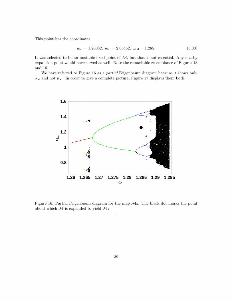
This point has the coordinates

qbd = 1.26082, pbd = 2.05452, ωbd = 1.285. (6.33)

It was selected to be an unstable fixed point of M, but that is not essential. Any nearbyexpansion point would have served as well. Note the remarkable resemblance of Figures 13and 16.

We have referred to Figure 16 as a partial Feigenbaum diagram because it shows onlyq∞ and not p∞. In order to give a complete picture, Figure 17 displays them both.

1.26 1.265 1.27 1.275 1.28 1.285 1.29 1.295Ω

0.8

1

1.2

1.4

1.6

q¥

Figure 16: Partial Feigenbaum diagram for the map M8. The black dot marks the pointabout which M is expanded to yield M8

.

39

Figure 17: Full Feigenbaum diagram for the map M8. The black dot again marks theexpansion point.

40

6.2.2 Strange Attractor

As displayed in Figures 18 through 21 M8, like M, appears to have a strange attractor.Note the remarkable agreement between Figures 14 and 15 for M and their M8 coun-terparts, Figures 18 and 19. In the case of M8 we have been able to obtain additionalenlargements, Figures 20 and 21, further illustrating a self-similar fractal structure. Analo-gous figures are more difficult to obtain for the exact mapM due to the excessive numericalintegration time required. By contrast the map M8, because it is a simple polynomial, iseasy to evaluate repeatedly.

Figure 18: Limiting values of q∞, p∞ for the map M8 when ω = 1.2902. They appear tolie on a strange attractor.

41

Figure 19: Enlargement of boxed portion of Figure 18 illustrating the beginning of self-similar fractal structure.

42

1.519 1.52 1.521 1.522 1.523q¥

2.014

2.015

2.016

2.017

2.018

2.019

2.02

2.021

p¥

Figure 20: Enlargement of boxed portion of Figure 19 illustrating the continuation ofself-similar fractal structure.

43

1.522 1.5221 1.5222 1.5223q¥

2.0172

2.0174

2.0176

2.0178

2.018

2.0182

2.0184

p¥

Figure 21: Enlargement of boxed portion of Figure 20 illustrating the further continuationof self-similar fractal structure.

44

7 Numerical Implementation

The forward integration method (Section 3.1) can be implemented by a code employingthe tools of automatic differentiation (AD) described by Neidinger [7].9 In this approacharrays of Taylor coefficients of various functions are referred to as AD variables or pyramidssince, as will be seen, they have a hyper-pyramidal structure. Generally the first entry inthe array will be the value of the function about some expansion point, and the remainingentries will be the higher-order Taylor coefficients about the expansion point and truncatedbeyond some specified order. Such truncated Taylor expansions are also commonly calledjets.

In our application elements in these arrays will be addressed and manipulated with theaid of scalar indices associated with look-up tables generated at run time. We have alsoreplaced the original APL implementation of Neidinger with a code written in the languageof Mathematica (Version 6, or 7) [8]. Where necessary, for those unfamiliar with the detailsof Mathematica, we will explain the consequences of various Mathematica commands. Theinputs to the code are the right sides (RS) of (1.1), or (2.1). Other input parameters arethe number of variables m, the desired order of the Taylor map p, and the initial conditions(zda)i for the design-solution equation (2.3).

Various AD tools for describing and manipulating pyramids are outlined in Section7.1. There we show how pyramid operations are encoded in the case of polynomial RS,as needed for the Duffing equation. For brevity, we omit the cases of rational, fractionalpower, and transcendental RS. These cases can also be handled using various methodsbased on functional identities and known Taylor coefficients, or the differential equationsthat such functions obey along with certain recursive relations [7]. In Section 7.2, based onthe work of Section (7.1), we in effect obtain and integrate numerically the set of differentialequations (3.6) in pyramid form, i.e. valid for any map order and any number of variables.Section 7.3 treats the specific case of the Duffing equation. A final Section 7.4 describesin more detail the relation between integrating equations for pyramids and the completevariational equations.

7.1 AD tools

This section describes how arithmetic expressions representing fa(z, t), the right sides of(1.1) where z denotes the dependent variables, are replaced with expressions for arrays(pyramids) of Taylor coefficients. These pyramids in turn constitute the input to our code.Such an ad-hoc replacement, according to the problem at hand, as opposed to operatoroverloading where the kind of operation depends on the type of its argument, is also theapproach taken in [7,9,10].

9Some authors refer to AD as truncated power series algebra (TPSA) since AD algorithms arise frommanipulating multivariable truncated power series. Other authors refer to AD as Differential Algebra (DA).

45

Let u, v, w be general arithmetic expressions, i.e. scalar-valued functions of z. Theycontain various arithmetic operations such as addition, multiplication (∗), and raising to apower (∧). (They may also entail the computation of various transcendental functions suchas the sine function, etc. However, as stated earlier, for simplicity we will omit these cases.)The arguments of these operations may be a constant, a single variable or multiple variablesza, or even some other expression. The idea of AD is to redefine the arithmetic operationsin such a way (see Definition 1), that all functions u, v, w can be consistently replaced withthe arrays of coefficients of their Taylor expansions. For example, by redefining the usualproduct of numbers (∗) and introducing the pyramid operation PROD, u∗v is replaced withPROD[U,V].

We use upper typewriter font for pyramids (U,V,...) and for operations on pyramids(PROD, POW, ...). Everywhere, equalities written in typewriter fonts have equivalentMathematica expressions. That is, they have associated realizations in Mathematica anddirectly correspond to various operations and commands in Mathematica. In effect, ourcode operates entirely on pyramids. However, as we will see, any pyramid expressioncontains, as its first entry, its usual arithmetic counterpart.

We begin with a description of our method of monomial labeling. In brief, we listall monomials in a polynomial in some sequence, and label them by where they occur inthe list. Next follow Definition 1 and the recipes for encoding operations on pyramids.Subsequently, by using Definition 2, which simply states the rule by which an arithmeticexpressions is replaced with its pyramid counterpart, we show how a general expressioncan be encoded by using only the pyramid of a constant and of a single variable.

7.1.1 Labeling Scheme

A monomial Gj(z) in m variables is of the form

Gj(z) = (z1)j1(z2)j2 · · · (zm)jm . (7.1)

Here we have introduced an exponent vector j by the rule

j = (j1, j2, · · · jm). (7.2)

Evidently j is an m-tuple of non-negative integers. The degree of Gj(z), denoted by |j|,is given by the sum of exponents,

|j| = j1 + j2 + · · ·+ jm. (7.3)

The set of all exponents for monomials in m variables with degree less than or equal to pwill be denoted by Γp

m,Γpm = j | |j| ≤ p. (7.4)

46

It can be shown that this set has L(m, p) entries with L(m, p) given given by a binomialcoefficient,

L(m, p) =

(p+m

p

). (7.5)

In [6] this quantity is called S0(m, p). Assuming that m and p are fixed input variables, wewill often write Γ and L. With this notation, a Taylor series expansion (about the origin)of a scalar-valued function u of m variables z = (z1, z2, . . . zm), truncated beyond terms ofdegree p, can be written in the form

u(z) =∑

j ∈ Γpm

U(j) Gj(z). (7.6)

Here, for now, U simply denotes an array of numerical coefficients. When employed in codethat has symbolic manipulation capabilities, each U(j) may also be a symbolic quantity.

To proceed, what is needed is some way of listing monomials systematically. Withsuch a list, as already mentioned, we may assign a label r to each monomial based onwhere it appears in the list. A summary of labeling methods, and an analysis of storagerequirements, may be found in [6,9]. Here we describe one of them that is particularlyuseful for our purposes.

The first step is to order the monomials or, equivalently, the exponent vectors. Onepossibility is lexicographic (lex) order. Consider two exponent vectors j and k. Let j − kbe the vector whose entries are obtained by component-wise subtraction,

j − k = (j1 − k1, j2 − k2, · · · jm − km). (7.7)

We say that the exponent vector j is lexicographically greater than the exponent vectork, and write j >lex k, if the left-most nonzero entry in j−k is positive. Thus, for examplein the case of monomials in three variables (z1, z2, z3) with exponents (j1, j2, j3), we havethe ordering

(1, 0, 0) >lex (0, 1, 0) >lex (0, 0, 1) (7.8)

and(4, 2, 1) >lex (4, 2, 0) >lex (2, 5, 1). (7.9)

For our purposes we have found it convenient to label the monomials in such a way thatmonomials of a given degree D = |j| occur together. One possibility is to employ gradedlexicographic (glex) ordering. If j and k are two exponent vectors, we say that j >glex k ifeither |j| > |k|, or |j| = |k| and j >lex k.

Table 4 shows a list of monomials in three variables. As one goes down the list, firstthe monomial of degree D = 0 appears, then the monomials of degree D = 1, etc. Withineach group of monomials of fixed degree the individual monomials appear in descendinglex order. Note that Table 4 is similar to Table 3 except that it begins with the monomialof degree 0.

47

Table 4: A labeling scheme for monomials in three variables.

r j1 j2 j3 D

1 0 0 0 02 1 0 0 13 0 1 0 14 0 0 1 15 2 0 0 26 1 1 0 27 1 0 1 28 0 2 0 29 0 1 1 210 0 0 2 211 3 0 0 312 2 1 0 313 2 0 1 314 1 2 0 315 1 1 1 316 1 0 2 317 0 3 0 318 0 2 1 319 0 1 2 320 0 0 3 3. . . . .. . . . .. . . . .

28 1 2 1 4. . . . .. . . . .. . . . .

We give the name modified glex sequencing to a monomial listing of the kind shown inTable 4. This is the labeling scheme we will use. Other possible listings include ascendingtrue glex order in which monomials appear in ascending lex order within each group ofdegree D, and lex order for the whole monomial list as in [7].

With the aid of the scalar index r the relation (7.6) can be rewritten in the form

u(z) =

L(m,p)∑r=1

U(r)Gr(z), (7.10)

48

because (by construction and with fixed m) for each positive integer r there is a uniqueexponent j(r), and for each j there is a unique r. Here U may be viewed as a vector withentries U(r), and Gr(z) denotes Gj(r)(z).

Consider, in an m-dimensional space, the points defined by the vectors j ∈ Γpm. See

(7.4). Figure 22 displays them in the case m = 3 and p = 4. Evidently they form a gridthat lies on the surface and interior of what can be viewed as an m-dimensional pyramid inm-dimensional space. At each grid point there is an associated coefficient U(r). Because ofits association with this pyramidal structure, we will refer to the entire set of coefficientsin (7.6) or (7.10) as the pyramid U of u(z).

01234

j1

01234

j2

0

1

2

3

4

j3

Figure 22: A grid of points representing the set Γ43. For future reference a subset of Γ4

3,called a box, is shown in blue.

7.1.2 Implementation of Labeling Scheme

We have seen that use of modified glex sequencing, for any specified number of variablesm, provides a labeling rule such that for each positive integer r there is a unique exponentj(r), and for each j there is a unique r. That is, there is a invertible function r(j) thatprovides a 1-to-1 correspondence between the positive integers and the exponent vectors j.To proceed further, it would be useful to have this function and its inverse in more explicitform.

First, we will learn that there is a formula for r(j), which we will call the Giorgilliformula [6]. For any specified m the exponent vectors j take the form (7.2) where all theentries ji are positive integers or zero. Begin by defining the integers

n(`; j1, · · · , jm) = `− 1 +`−1∑k=0

jm−k (7.11)

49

for ` ∈ 1, 2, · · ·m. Then, to the general monomial Gj(z) or exponent vector j, assignthe label

r(j) = r(j1, · · · jm) = 1 +m∑`=1

Binomial [n(`; j1, · · · jm), `]. (7.12)

Here the quantities

Binomial [n, `] =

(n`

)=

n!

`!(n−`)! , 0 ≤ ` ≤ n0 , otherwise

(7.13)

denote the usual binomial coefficients. It can be shown that this formula reproduces theresults of modified glex sequencing [6].

Below is simple Mathematica code that implements the Giorgilli formula in the case ofthree variables, and evaluates it for selected exponents j. Observe that these evaluationsagree with results in Table 4.

Gfor[j1 , j2 , j3 ] := (

s1 = j3; s2 = 1 + j3 + j2; s3 = 2 + j3 + j2 + j1;

t1 = Binomial[s1, 1]; t2 = Binomial[s2, 2]; t3 = Binomial[s3, 3];

r = 1 + t1 + t2 + t3; r

)

Gfor[0, 0, 0]

Gfor[1, 0, 0]

Gfor[2, 0, 1]

Gfor[1, 2, 1]

1

2

13

28 (7.14)

Second, for the inverse relation, we have found it convenient to introduce a rectangularmatrix associated with the set Γp

m. By abuse of notation, it will also be called Γ. It hasL(m, p) rows and m columns with entries

Γr,a = ja(r). (7.15)

For example, looking a Table 4, we see (when m = 3) that Γ1,1 = 0 and Γ17,2 = 3. Indeed,if the first and last columns of Table 4 are removed, what remains (when m = 3) is thematrix Γr,a. In the language of [6], Γ is a look up table that, given r, produces the associatedj. In our Mathematica implementation Γ is the matrix GAMMA with elements GAMMA[[r, a]].

50

The matrix GAMMA is constructed using the Mathematica code illustrated below,

Needs["Combinatorica‘"];

m = 3; p = 4;

GAMMA = Compositions[0, m];

Do[GAMMA = Join[GAMMA, Reverse[Compositions[d, m]]], d, 1, p, 1];L = Length[GAMMA]

r = 17; a = 2;

GAMMA[[r]]

GAMMA[[r, a]]

35

0, 3, 03 (7.16)

It employs the Mathematica commands Compositions, Reverse, and Join.We will first describe the ingredients of this code and illustrate the function of each:

• The command Needs["Combinatorica‘"]; loads a combinatorial package.

• The command Compositions[i, m] produces, as a list of arrays (a rectangular array),all compositions (under addition) of the integer i into m integer parts. Further-more, the compositions appear in ascending lex order. For example, the commandCompositions[0, 3] produces the single row

0 0 0 (7.17)

As a second example, the command Compositions[1, 3] produces the rectangulararray

0 0 1

0 1 0

1 0 0 (7.18)

As a third example, the command Compositions[2, 3] produces the rectangular array

0 0 2

0 1 1

0 2 0

1 0 1

1 1 0

2 0 0 (7.19)

51

• The command Reverse acts on the list of arrays, and reverses the order of the listwhile leaving the arrays intact. For example, the nested sequence of commandsReverse[Compositions[1, 3]] produces the rectangular array

1 0 0

0 1 0

0 0 1 (7.20)

As a second example, the nested sequence of commands Reverse[Compositions[2, 3]]produces the rectangular array

2 0 0

1 1 0

1 0 1

0 2 0

0 1 1

0 0 2 (7.21)

Now the compositions appear in descending lex order.

• Look, for example, at Table 4. We see that the exponents ja for the r = 1 entryare those appearing in (7.17). Next, exponents for the r = 2 through r = 4 entriesare those appearing in (7.20). Following them, the exponents for the r = 5 throughr = 10 entries, are those appearing in (7.21), etc. Evidently, to produce the exponentlist of Table 4, what we must do is successively join various lists. That is what theMathematica command Join can accomplish.

We are now ready to describe how GAMMA is constructed:

• The second line in (7.16) sets the values of m and p. They are assigned the valuesm = 3 and p = 4 for this example, which will construct GAMMA for the case of Table 4.The third line in (7.16) initially sets GAMMA to a row of m zeroes. The fourth line isa Do loop that successively redefines GAMMA by generating and joining to it successivedescending lex order compositions. The net result is the exponent list of Table 4.

• The quantity L = L(m, p) is obtained by applying the Mathematica command Length

to the the rectangular array GAMMA.

• The last 6 lines of (7.16) illustrate that L is computed properly and that the com-mand GAMMA[[r, a]] accesses the array GAMMA in the desired fashion. Specifically, inthis example, we find from (7.5) that L(3, 4) = 35 in agreement with the Mathe-matica output for L. Moreover, GAMMA[[17]] produces the exponent array 0, 3, 0, inagreement with the r = 17 entry in Table 4, and GAMMA[[17, 2]] produces Γ17,2 = 3,as expected.

52

7.1.3 Pyramid Operations: Addition and Multiplication

Here we derive the pyramid operations in terms of j-vectors by using the ordering previouslydescribed, and provide scripts to encode them in the r-representation (7.10).

Definition 1 Suppose that w(z) arises from carrying out various arithmetic operations onu(z) and v(z), and the pyramids U and V are known. The corresponding pyramid operationon U and V is so defined that it yields the pyramid W of w(z).

Here we assume that u, v, w are polynomials such as (7.6).We begin with the operations of scalar multiplication and addition, which are easy to

implement. Ifw(z) = c u(z), (7.22)

thenW(r) = c U(r), (7.23)

and we writeW = c U. (7.24)

Ifw(z) = u(z) + v(z), (7.25)

thenW(r) = U(r) + V(r), (7.26)

and we writeW = U + V. (7.27)

In both cases all operations are performed coordinate-wise (as for vectors).Implementation of scalar multiplication and addition is easy in Mathematica because, as

the example below illustrates, it has built in vector routines. There we define two vectors,multiply them by scalars, and add the resulting vectors.

Unprotect[V];

U = 1, 2, 3;V = 4, 5, 6;W = .1U + .2V

.9, 1.2, 1.5 (7.28)

Since V is a “protected” symbol in the Mathematica language, and, for purposes of illus-tration, we wish to use it as an ordinary vector variable, it must first be unprotected as inline 1 above. The last line shows that the Mathematica output is indeed the desired result.

The operation of polynomial multiplication is more involved. Now we have the relation

w(z) = u(z) ∗ v(z), (7.29)

53

and we want to encodeW = PROD[U, V]. (7.30)

Let us write u(x) in the form (7.6), but with a change of dummy indices, so that it hasthe representation

u(z) =∑

i ∈ Γpm

U(i) Gi(z). (7.31)

Similarly, write v(z) in the form

v(z) =∑

j ∈ Γpm

V(j) Gj(z). (7.32)

Then, according to Leibniz, there is the result

u(z) ∗ v(z) =∑

i ∈ Γpm

∑j ∈ Γp

m

U(i)V(j)Gi(z) ∗Gj(z). (7.33)

From (7.1) we observe that

Gi(z) ∗Gj(z) = (z1)i1(z2)i2 · · · (zm)im ∗ (z1)j1(z2)j2 · · · (zm)jm

= (z1)i1+j1(z2)i2+j2 · · · (zm)im+jm = Gi+j(z). (7.34)

Therefore, we may also write

u(z) ∗ v(z) =∑

i ∈ Γpm

∑j ∈ Γp

m

U(i)V(j)Gi+j(z). (7.35)

Now we see that there are two complications. First, there may be terms on the right sideof (7.35) whose degree is higher than p and therefore need not be computed. Second, thereare generally many terms on the right side of (7.35) that contribute to a given monomialterm in w(z) = u(z) ∗ v(z). Suppose we write

w(z) =∑k

W(k) Gk(z). (7.36)

Upon comparing (7.35) and (7.36) we conclude that

W(k) =∑

i+j=k

U(i)V(j) =∑j≤k

U(k − j)V(j). (7.37)

Here, by j ≤ k, we mean that the sum ranges over all j such that ja ≤ ka for all a ∈ [1,m].That is,

j ≤ k ⇔ ja ≤ ka for all a ∈ [1,m]. (7.38)

54

Evidently, to implement the relation (7.37) in terms of r labels, we need to describethe exponent relation j ≤ k in terms of r labels. Suppose k is some exponent vector withlabel r(k) as, for example, in Table 4. Introduce the notation

k = r(k). (7.39)

This notation may be somewhat confusing because k is not the norm of the vector k, butrather the label associated with k. However, this notation is very convenient. Now, givena label k, we can find k. Indeed, from (7.15), we have the result

ka = Γk,a. (7.40)

Having found k, we define a set of exponents Bk by the rule

Bk = j|j ≤ k. (7.41)

This set of exponents is called the kth box. For example (when m = 3), suppose k = 28.Then we see from Table 4 that k = (1, 2, 1). Table 5 lists, in modified glex order, all thevectors in B28, i.e. all vectors j such that j ≤ (1, 2, 1). These are the vectors shown inblue in Figure 22. Finally, with this notation, we can rewrite (7.37) in the form

W(k) =∑j∈Bk

U(k − j)V(j). (7.42)

Table 5: The vectors in B28 = j|j ≤ (1, 2, 1).

r j1 j2 j3 D

1 0 0 0 02 1 0 0 13 0 1 0 14 0 0 1 16 1 1 0 27 1 0 1 28 0 2 0 29 0 1 1 214 1 2 0 315 1 1 1 318 0 2 1 328 1 2 1 4

What can be said about the vectors (k − j) as j ranges over B`? Table 6 lists, forexample, the vectors j ∈ B28 and the associated vectors i with i = (k − j). Also listed are

55

the labels r(j) and r(i). Compare columns 2,3,4, which specify the j ∈ B28, with columns5,6,7, which specify the associated i vectors. We see that every vector that appears in thej list also occurs somewhere in the i list, and vice versa. This to be expected because theoperation of multiplication is commutative: we can also write (7.37) in the form

W(k) =∑j∈Bk

U(j)V(k − j). (7.43)

We also observe the more remarkable feature that the two lists are reverses of each other:running down the j list gives the same vectors as running up the i list, and vice versa.This feature is a consequence of our ordering procedure.

As indicated earlier, what we really want is a version of (7.37) that involves labelsinstead of exponent vectors. Looking at Table 6, we see that this is easily done. We mayequally well think of Bk as containing a collection of labels r(j), and we may introduce areversed array Brevk of complementary labels rc(j) where

rc(j) = r(i). (7.44)

That is, for example, B28 would consist of the first column of Table 6 and Brev28 wouldconsist of the last column of Table 6. Finally, we have already introduced k as being thelabel associated with k. We these understandings in mind, we may rewrite (7.37) in thelabel form

W(k) =∑r∈Bk

U(rc)V(r) =∑r∈Bk

U(r)V(rc). (7.45)

This is the rule W = PROD[U, V] for multiplying pyramids. In the language of [6], Bk andBrevk are look back tables that, given a k, look back to find all monomial pairs with labelsr, rc which produce, when multiplied, the monomial with label k.

7.1.4 Implementation of Multiplication

The code shown below in (7.46) illustrates how Bk and Brevk are constructed using Math-ematica.

JSK[list , K ] :=

Position[Apply[And, Thread[#1<=#2&[#,K]]]& /@ list, True]//Flatten;

B = Table[JSK[GAMMA, GAMMA[[k]]], k, 1, L];Brev = Reverse /@ B; (7.46)

As before, some explanation is required. The main tasks are to implement the j ≤ koperation (7.38) and then to employ this implementation. We will begin by implementingthe j ≤ k operation. Several steps are required, and each of them is described brieflybelow:

56

Table 6: The vectors j and i = (k − j) for j ∈ B28 and ka = Γ28,a.

r(j) j1 j2 j3 i1 i2 i3 r(i)

1 0 0 0 1 2 1 282 1 0 0 0 2 1 183 0 1 0 1 1 1 154 0 0 1 1 2 0 146 1 1 0 0 1 1 97 1 0 1 0 2 0 88 0 2 0 1 0 1 79 0 1 1 1 1 0 614 1 2 0 0 0 1 415 1 1 1 0 1 0 318 0 2 1 1 0 0 228 1 2 1 0 0 0 1

• When Mathematica is presented with a statement of the form j <= k, with j andk being integers, it replies with the answer True or the answer False. (Here j <= kdenotes j ≤ k.) Two sample Mathematica runs are shown below:

3 <= 4

True (7.47)

5 <= 4

False (7.48)

• A Mathematica function can be constructed that does the same thing. It takes theform

#1 <= #2 & [j, k] (7.49)

Here the symbols #1 and #2 set up two slots and the symbol & means the operationto its left is to be regarded as a function and is to be applied to the arguments toits right by inserting the arguments into the slots. Below is a short Mathematica runillustrating this feature.

j = 3; k = 4;

#1 <= #2 & [j, k]

True (7.50)

Observe that the output of this run agrees with that of (7.47).

57

• The same operation can be performed on pairs of arrays (rather than pairs of num-bers) in such a way that corresponding entries from each array are compared, withthe output then being an array of True and False answers. This is done using theMathematica command Thread. Below is a short Mathematica run illustrating thisfeature.

j = 1, 2, 3; k = 4, 5, 1;Thread[#1 <= #2 & [j, k]]

True,True,False (7.51)

Note that the first two answers in the output array are True because the statements1 ≤ 4 and 2 ≤ 5 are true. The last answer in the output array is False because thestatement 3 ≤ 1 is false.

• Suppose, now, that we are given two arrays j and k and we want to determine ifj ≤ k in the sense of (7.38). This can be done by applying the logical And operation(using the Mathematica command Apply) to the True/False output array describedabove. Below is a short Mathematica run illustrating this feature.

j = 1, 2, 3; k = 4, 5, 1;Apply[And, Thread[#1 <= #2 & [j, k]]]

False (7.52)

Note that the output answer is False because at least one of the entries in the outputarray in (7.51) is False. The output answer would be True if, and only if, all entriesin the output array in (7.51) were True.

• Now that the j ≤ k operation has been defined for two exponent arrays, we wouldlike to construct a related operator/function, to be called JSK. (Here the letter S

stands for smaller than or equal to.) It will depend on the exponent array k, and itstask will be to search a list of exponent arrays to find those j within it that satisfyj ≤ k. The first step in this direction is to slightly modify the function appearing in(7.52). Below is a short Mathematica run that specifies this modified function andillustrates that it has the same effect.

j = 1, 2, 3; k = 4, 5, 1;Apply[And, Thread[#1 <= #2 & [#, k]]] & [j]

False (7.53)

Comparison of the functions in (7.52) and (7.53) reveals that what has been done is toreplace the argument j in (7.52) by a slot #, then follow the function by the character&, and finally add the symbols [j]. What this modification does is to redefine thefunction in such a way that it acts on what follows the second &.

58

• The next step is to extend the function appearing in (7.53) so that it acts on a list ofexponent arrays. To do this, we replace the symbols [j] by the symbols /@ list. Thesymbols /@ indicate that what stands to their left is to act on what stands to theirright, and what stands to their right is a list of exponent arrays. The result of thisaction will be a list of True/False results with one result for each exponent array inthe list. Below is a short Mathematica run that illustrates how the further modifiedfunction acts on lists.

k = 4, 5, 1;ja = 3, 4, 1; jb = 1, 2, 3; jc = 1, 2, 1;list = ja, jb, jc;Apply[And, Thread[#1 <= #2 & [#, k]]] & /@ list

True,False,True (7.54)

Observe that the output answer list is True,False,True because 3, 4, 1 ≤ 4, 5, 1is True, 1, 2, 3 ≤ 4, 5, 1 is False, and 1, 2, 1 ≤ 4, 5, 1 is True.

• What we would really like to know is where the True items are in the list, becausethat will tell us where the j that satisfy j ≤ k reside. This can be accomplishedby use of the Mathematica command Position in conjunction with the result True.Below is a short Mathematica run that illustrates how this works.

k = 4, 5, 1;ja = 3, 4, 1; jb = 1, 2, 3; jc = 1, 2, 1;list = ja, jb, jc;Position[Apply[And, Thread[#1 <= #2 & [#, k]]] & /@ list, True]

1, 3 (7.55)

Note that the output is an array of positions in the list for which j ≤ k. Thereis, however, still one defect. Namely, the output array is an array of single-elementsubarrays, and we would like it to be simply an array of location numbers. This defectcan be remedied by appending the Mathematica command Flatten, preceded by //,to the instruction string in (7.55). The short Mathematica run below illustrates thismodification.

k = 4, 5, 1;ja = 3, 4, 1; jb = 1, 2, 3; jc = 1, 2, 1;list = ja, jb, jc;Position[Apply[And, Thread[#1 <= #2 & [#, k]]] & /@ list, True]//Flatten

1, 3 (7.56)

Now the output is a simple array containing the positions in the list for which j ≤ k.

59

• The last step is to employ the ingredients in (7.56) to define the operator JSK[list, k].The short Mathematica run below illustrates how this can be done.

k = 4, 5, 1;ja = 3, 4, 1; jb = 1, 2, 3; jc = 1, 2, 1;list = ja, jb, jc;JSK[list , k ] :=

Position[Apply[And, Thread[#1 <= #2 & [#, k]]] & /@ list, True]//Flatten;

JSK[list, k]

1, 3 (7.57)

Lines 4 and 5 above define the operator JSK[list, k], line 6 invokes it, and line 7displays its output, which agrees with the output of (7.56).

• With the operator JSK[list, k] in hand, we are prepared to construct tables B andBrev that will contain the Bk and the Brevk. The short Mathematica run belowillustrates how this can be done.

B = Table[JSK[GAMMA, GAMMA[[k]]], k, 1, L, 1];Brev = Reverse /@ B;

B[[8]]

Brev[[8]]

B[[28]]

Brev[[28]]

1, 3, 88, 3, 11, 2, 3, 4, 6, 7, 8, 9, 14, 15, 18, 2828, 18, 15, 14, 9, 8, 7, 6, 4, 3, 2, 1 (7.58)

The first line employs the Mathematica command Table in combination with animplied Do loop to produce a two-dimensional array B. Values of k in the range [1, L]are selected sequentially. For each k value the associated exponent array k(k) =GAMMA[[k]] is obtained. The operator JSK then searches the full GAMMA array to findthe list of r values associated with the j ≤ k. All these r values are listed in a row.Thus, the array B consists of list of L rows, of varying width. The rows are labeled byk ∈ [1, L], and in each row are the r values associated with the j ≤ k. In the secondline the Mathematica command Reverse is applied to B to produce a second arraycalled Brev. Its rows are the reverse of those in B. For example, as the Mathematica

60

run illustrates, B[[8]], which is the 8th row of B, contains the list 1, 3, 8, and Brev[[8]]contains the list 8, 3, 1. Inspection of the r = 8 monomial in Table 4, that withexponents 0, 2, 0, shows that it has the monomials with exponents 0,0,0, 0,1,0,and 0,2,0 as factors. And further inspection of Table 4 shows that the exponentsof these factors have the r values 1, 3, 8. Similarly B[[28]], which is the 28th rowof B, contains the same entries that appear in the first column of Table 6. AndBrev[[28]], which is the 28th row of Brev, contains the same entries that appear inthe last column of Table 6.

Finally, we need to explain how the arrays B and Brev can be employed to carry outpolynomial multiplication. This can be done using the Mathematica dot product command:

• The exhibit below shows a simple Mathematica run that illustrates the use of the dotproduct command.

Unprotect[V];

U = .1, .2, .3, .4, .5, .6, .7, .8;V = 1.1, 1.2, 1.3, 1.4, 1.5, 1.6, 1.7, 1.8;U.V

u = 1, 3, 5;v = 6, 4, 2;U[[u]]

V[[v]]

U[[u]].V[[v]]

5.64

.1, .3, .51.6, 1.4, 1.21.18 (7.59)

As before, V must be unprotected. See line 1. The rest of the first part this run (lines2 through 4) defines two vectors U and V and then computes their dot product. Notethat if we multiply the entries in U and V pairwise and add, we get the result

.1× 1.1 + .2× 1.2 + · · ·+ .8× 1.8 = 5.64,

which agrees with the Mathematica result for U · V. See line 10.

The second part of this Mathematica run, lines 5 through 9, illustrates a powerfulfeature of the Mathematica language. Suppose, as illustrated, we define two arrays uand v of integers, and use these arrays as arguments for the vectors by writing U[[u]]and V[[v]]. Then Mathematica uses the integers in the two arrays u and v as labels

61

to select the corresponding entries in U and V, and from these entries it makes newcorresponding vectors. In this example, the 1st, 3rd, and 5th entries in U are .1, .3,and .5. And the 6th, 4th, and 2nd entries in V are 1.6, 1.4, and 1.2. Consequently, wefind that

U[[u]] = .1, .3, .5,

V[[v]] = 1.6, 1.4, 1.2,

in agreement with lines 11 and 12 of the Mathematica results. Correspondingly, weexpect that U[[u]] · V[[v]] will have the value

U[[u]] · V[[v]] = .1× 1.6 + .3× 1.4 + .5× 1.2 = 1.18,

in agreement with the last line of the Mathematica output.

• Now suppose, as an example, that we set k = 8 and use B[[k]] and Brev[[k]] in placeof the arrays u and v. The Mathematica fragment below shows what happens whenthis is done.

k = 8;

B[[k]]

Brev[[k]]

U[[B[[k]]]]

V[[Brev[[k]]]]

U[[B[[k]]]] · B[[Brev[[k]]]]

1, 3, 88, 3, 1.1, .3, .81.8, 1.3, 1.11.45 (7.60)

From (7.58) we see that B[[8]] = 1, 3, 8 and Brev[[8]] = 8, 3, 1 in agreement withlines 7 and 8 of the Mathematica output above. Also, the 1st, 3rd, and 8th entriesin U are .1, .3, and .8. And the 8th, 3rd, and 1st entries in V are 1.8, 1.3, and 1.1.Therefore we expect the results

U[[B[[k]]]] = .1, .3, .8,

V[[Brev[[k]]]] = 1.8, 1.3, 1.1,

U[[B[[k]]]] · V[[Brev[[k]]]] = .1× 1.8 + .3× 1.3 + .8× 1.1 = 1.45,

in agreement with the last three lines of (7.60).

62

• Finally, suppose we carry out the operation U[[B[[k]]]] · V[[Brev[[k]]]] for all k ∈ [1, L]and put the results together in a Table with entries labeled by k. According to(7.45), the result will be the pyramid for the product of the two polynomials whoseindividual pyramids are U and V. The Mathematica fragment below shows how thiscan be done to define a product function, called PROD, that acts on general pyramidsU and V, using the command Table with an implied Do loop over k.

PROD[U , V ] := Table[U[[B[[k]]]] · V[[Brev[[k]]]], k, 1, L, 1];

7.1.5 Implementation of Powers

With operation of multiplication in hand, it is easy to implement the operation of raising apyramid to a power. The code shown below in (7.61) demonstrates how this can be done.

POWER[U , 0] := C1;

POWER[U , 1] := U;

POWER[U , 2] := PROD[U, U];

POWER[U , 3] := PROD[U, POWER[U, 2]];

... (7.61)

Here C1 is the pyramid for the Taylor series having one as its constant term and all otherterms zero,

C1 = 1, 0, 0, 0, · · · . (7.62)

It can be set up by the Mathematica code

C1 = Table[KroneckerDelta[k, 1], k, 1, L, 1]; (7.63)

which employs the Table command, the Kronecker delta function, and an implied Do loopover k. This code should be executed before executing (7.61), but after the value of L hasbeen established.

7.1.6 Replacement Rule

Definition 2 The transformation A(z) A means replacement of every real variable zain the arithmetic expression A(z) with an associated pyramid, and of every operation onreal variables in A(z) with the associated operation on pyramids.

Automatic Differentiation is based on the following corollary: if A(z) A, then A is thepyramid of A(z).

For simplicity, we will begin our discussion of the replacement rule with examplesinvolving only a single variable z. In this case monomial labeling, the relation betweenlabels and exponents, is given directly by the simple rules

r(j) = 1 + j and j(r) = r − 1. (7.64)

63

Table 7: A labeling scheme for monomials in one variable.

r j

1 02 13 24 3· ·· ·

See table 7.As a first example, consider the expression

A = 2 + 3(z ∗ z). (7.65)

We have agreed to consider the case m = 1. Suppose we also set p = 2, in which caseL = 3. In ascending glex order, see Table 7, the pyramid for A is then

2 + 3z2 A = (2, 0, 3). (7.66)

Now imagine that A was not such a simple polynomial, but some complicated expression.Then the pyramid A could be generated by computing derivatives of A at z = 0 and dividingthem by the appropriate factorials. Automatic differentiation offers another way to find A.Assume that all operations in the arithmetic expression A have been encoded accordingto Definition 1. For our example, these are + and PROD. Let C1 and Z be the pyramidsassociated with 1 and z,

1 C1 = (1, 0, 0), (7.67)

z Z = (0, 1, 0). (7.68)

The quantity 2 + 3z2 results from performing various arithmetic operations on 1 and z.Definition 1 says that the pyramid of 2 + 3z2 is identical to the pyramid obtained byperforming the same operations on the pyramids C1 and Z. That is, suppose we replace 1and z with correctly associated pyramids C1 and Z, and also replace ∗ with PROD. Then,upon evaluating PROD, multiplying by the appropriate scalar coefficients, and summing,the result will be the same pyramid A,

2 C1 + 3 PROD[Z, Z] = A. (7.69)

In this way, by knowing only the basic pyramids C1 and Z (prepared beforehand), one cancompute the pyramid of an arbitrary A(z). Finally, in contrast to numerical differentiation,

64

all numerical operations involved are accurate to machine precision. Mathematica code thatimplements (7.69) will be presented shortly in (7.70).

Frequently, if A(z) is some complicated expression, the replacement rule will resultin a long chain of nested pyramid operations. At every step in the chain, the pyramidresulting from the previous step will be combined with some other pyramid to produce anew pyramid. Each such operation has two arguments, and Definition 1 applies to eachstep in the chain. Upon evaluating all pyramid operations, the final result will be thepyramid of A(z).

By using the replacement operator the above procedure can be represented as:

1 C1, z Z, A A.

The following general recipe then applies: In order to derive the pyramid associated withsome arithmetic expression, apply the rule to all its variables, or parts, and replace alloperations with operations on pyramids. Here “apply the rule” to something meansreplace that something with the associated pyramid. And the term “parts” means sub-expressions. Definition 1 guarantees that the result will be the same pyramid A no matterhow we split the arithmetic expression A into sub-expressions. It is only necessary torecognize, in case of using sub-expressions, that one pyramid expression should be viewedas a function of another.

For illustration, suppose we regard the A given by (7.65) to be the composition of twofunctions, F (z) = 2 + 3z and G(z) = z2, so that A(z) = F (G(z)). Instead of associating aconstant and a single variable with their respective pyramids, let us now associate wholesub-expressions. In addition, let us label the pyramid expressions on the right of withwith some names, F and G:

2 + 3z 2 C1 + 3 Z = F[Z]

z2 PROD[Z, Z] = G[Z]

A(z) F[G[Z]] = A.

We have indicated the explicit dependence on Z. It is important to note that F[Z] isa pyramid expression prior to executing any the pyramid operations, i.e it is not yet apyramid, but is simply the result of formal replacements that follow the association rule.

Mathematica code for the simple example (7.69) is shown below,

C1 = 1, 0, 0;Z = 0, 1, 0;2 C1 + 3 PROD[Z, Z]

2, 0, 3 (7.70)

Note that the result (7.70) agrees with (7.66). This example does not use any nestedexpressions. We will now illustrate how the same results can be obtained using nestedexpressions.

65

We begin by displaying a simple Mathematica program/execution, that employs ordi-nary variables, and uses Mathematica’s intrinsic abilities to handle nested expressions. Theprogram/execution is

f[z ] := 2 + 3z;

g[z ] := z2;

f[g[z]]

2 + 3z2 (7.71)

With Mathematica the underscore in z indicates that z is a dummy variable name, andthe symbols := indicate that f is defined with a delayed assignment. That is what is donein line one above. The same is done in line two for g. Line three requests evaluation of thenested function f(g(z)), and the result of this evaluation is displayed in line four. Notethat the result agrees with (7.65).

With this background, we are ready to examine a program with analogous nestedpyramid operations. The same comments apply regarding the use of underscores anddelayed assignments. The program is

C1 = 1, 0, 0;Z = 0, 1, 0;F[Z ] := 2 C1 + 3 Z;

G[Z ] := PROD[Z, Z];

F[G[Z]]

2, 0, 3 (7.72)

Note that line (7.72) agrees with line (7.70), and is consistent with line (7.66).We close this subsection with an important consequence of the replacement rule and

nested operations, which we call the Taylor rule. We begin by considering functions of asingle variable. Suppose the function G(x) has the special form

G(x) = zd + x (7.73)

where zd is some constant. Let F be some other function. Consider the composite (nested)function A defined by

A(x) = F (G(x)) = F (zd + x). (7.74)

Then, assuming the necessary analyticity, by the chain rule A evidently has a Taylorexpansion in x about the origin of the form

A = A(0) +A′(0)x+ (1/2)A′′(0)x2 + · · ·= F (zd) + F ′(zd)x+ (1/2)F ′′(zd)x2 + · · · . (7.75)

66

We conclude that if we know the Taylor expansion of A about the origin, then we alsoknow the Taylor expansion of F about zd, and vice versa. Suppose, for example, that

F (z) = 1 + 2z + 3z2 (7.76)

andzd = 4. (7.77)

Then there is the result

A(x) = F (G(x)) = F (zd + x) = 1 + 2(4 + x) + 3(4 + x)2 = 57 + 26x+ 3x2. (7.78)

We now show that this same result can be obtained using pyramids. The Mathematicafragment below illustrates how this can be done.

C1 = 1, 0, 0;X = 0, 1, 0;zd = 4;

F[Z ] := 1 C1 + 2 Z + 3 PROD[Z, Z];

G[X ] := zd C1 + X;

F[G[X]]

57, 26, 3 (7.79)

Note that (7.79) agrees with (7.78).Let us also illustrate the Taylor rule in the two-variable case. Let F (z1, z2) be some

function of two variables. Introduce the functions G(x1) and H(x1) having the specialforms

G(x1) = zd1 + x1, (7.80)

H(x2) = zd2 + x2, (7.81)

where zd1 and zd2 are some constants. Consider the function A defined by

A(x1, x2) = F (G(x1), H(x2)) = F (zd1 + x1, zd2 + x2). (7.82)

Then, again assuming the necessary analyticity, by the chain rule A evidently has a Taylorexpansion in x1 and x2 about the origin (0, 0) of the form

A = A(0, 0) + [∂1A(0, 0)]x1 + [∂2A(0, 0)]x2

+(1/2)[(∂1)2A(0, 0)]x21 + [∂1∂2A(0, 0)]x1x2 + (1/2)[(∂2)2A(0, 0)]x2

2 + · · ·= F (zd1 , z

d2) + [∂1F (zd1 , z

d2)]x1 + [∂2F (zd1 , z

d2)]x2

+(1/2)[(∂1)2F (zd1 , zd2)]x2

1 + [∂1∂2AF (zd1 , zd2)]x1x2 + (1/2)[(∂2)2A(F (zd1 , z

d2))]x2

2 + · · ·(7.83)

67

where∂1 = ∂/∂x1, ∂2 = ∂/∂x2 (7.84)

when acting on A, and∂1 = ∂/∂z1, ∂2 = ∂/∂z2 (7.85)

when acting on F . We conclude that if we know the Taylor expansion of A about the origin(0, 0), then we also know the Taylor expansion of F about (zd1 , z

d2), and vice versa.

As a concrete example, suppose that

F (z1, z2) = 1 + 2z1 + 3z2 + 4z21 + 5z1z2 + 6z2

2 (7.86)

andzd1 = 7, zd2 = 8. (7.87)

Then, hand calculation shows that F (G(x1), H(x2)) takes the form

F (zd1 + x1, zd2 + x2) = F (G(x1), H(x2))

= 899 + 98x1 + 4x21 + 134x2 + 5x1x2 + 6x2

2. (7.88)

Below is a Mathematica execution that finds the same result,

F[z1 , z2 ] := 1 + 2 z1 + 3 z2 + 4 z12 + 5 z1 z2 + 6 z22

G[x1 ] := zd1 + x1;

H[x2 ] := zd2 + x2;

zd1 = 7;

zd2 = 8;

A = F[G[x1], H[x2]]

Expand[A]

1 + 2 (7 + x1) + 4 (7 + x1)2 + 3 (8 + x2) + 5 (7 + x1) (8 + x2) + 6 (8 + x2)2

899 + 98 x1 + 4 x12 + 134 x2 + 5 x1 x2 + x22

(7.89)

68

The calculation above dealt with the case of a function of two ordinary variables. Wenow illustrate, for the same example, that there is an analogous result for pyramids. Forfuture reference, Table 8 shows our standard modified glex sequencing applied to the caseof two variables.

Table 8: A labeling scheme for monomials in two variables.

r j1 j21 0 02 1 03 0 14 2 05 1 16 0 27 3 08 2 19 1 210 0 3· · ·· · ·

Following the replacement rule, we should make the substitutions

zd1 + x1 zd1 C1 + X1, (7.90)

zd2 + x2 zd2 C1 + X2, (7.91)

1 + 2 z1 + 3 z2 + 4 z21 + 5 z1 z2 + 6 z2

2

C1 + 2 Z1 + 3 Z2 + 4 PROD[Z1, Z1] + 5 PROD[Z1, Z2] + 6 PROD[Z2, Z2].

(7.92)

69

The Mathematica fragment below, executed for the case m = 2 and p = 2, in which caseL = 6, illustrates how the analogous result is obtained using pyramids,

C1 = 1, 0, 0, 0, 0, 0;X1 = 0, 1, 0, 0, 0, 0;X2 = 0, 0, 1, 0, 0, 0;F[Z1 , Z2 ] := C1 + 2 Z1 + 3 Z2 + 4 PROD[Z1, Z1] + 5 PROD[Z1, Z2]

+6 PROD[Z2, Z2];

G[X1 ] := z01 C1 + X1;

H[X2 ] := z02 C1 + X2;

zd1 = 7;

zd2 = 8;

F[G[X1], H[X2]]

899, 98, 134, 4, 5, 6 (7.93)

Note that, when use is made of Table 8, the last line of (7.93) agrees with (7.88) and thelast line of (7.89).

7.2 Replacement Rule and Numerical Integration

7.2.1 Numerical Integration

Consider the set of differential equations (1.5). A standard procedure for their numericalintegration from an initial time ti = t0 to some final time tf is to divide the time axis intoa large number of steps N , each of small duration h, thereby introducing successive timestn defined by the relation

tn = t0 + nh with n = 0, 1, · · · , N. (7.94)

By construction, there will also be the relation

Nh = tf − ti. (7.95)

The goal is to compute the vectors zn, where

zn = z(tn), (7.96)

starting from the vector z0. The vector z0 is assumed given as a set of definite numbers,i.e. the initial conditions at t0.

If we assume Poincare analyticity in t, we may convert the set of differential equations(1.5) into a set of recursion relations for the zn in such a way that the zn obtained by

70

solving the recursion relations differ from the true zn by only small truncation errors oforder hm. (Here m is not the number of variables, but rather some fixed integer describingthe accuracy of the integration method.) One such procedure, fourth-order Runge Kutta(RK4), is the set of marching/recursion rules

zn+1 = zn +1

6(a+ 2b+ 2c+ d) (7.97)

where, at each step,a = hf(zn, tn), (7.98)

b = hf(zn +1

2a, tn +

1

2h),

c = hf(zn +1

2b, tn +

1

2h),

d = hf(zn + c, tn + h).

Thanks to the genius of Runge and Kutta, the relations (7.97) and (7.98) have been con-structed in such a way that the method is locally (at each step) correct through order h4,and makes local truncation errors of order h5.

In the case of a single variable, and therefore a single differential equation, the relations(7.97) and (7.98) may be encoded in the Mathematica form shown below. Here Zvar is thedependent variable, t is the time, Zt is a temporary variable, tt is a temporary time, andns is the number of integration steps. The program employs a Do loop over i so that theoperations (7.97) and (7.98) are carried out ns times.

71

RK4 := (

t0 = t;

Do[

Aa = h F[Zvar, t];

Zt = Zvar + (1/2)Aa;

tt = t + h/2;

Bb = h F[Zt, tt];

Zt = Zvar + (1/2)Bb;

Cc = h F[Zt, tt];

Zt = Zvar + Cc;

tt = t + h;

Dd = h F[Zt, tt];

Zvar = Zvar + (1/6)(Aa + 2 Bb + 2 Cc + Dd);

t = t0 + i h;,

i, 1, ns, 1]

)

(7.99)

7.2.2 Replacement Rule, Single Equation/Variable Case

We now make what, for our purposes, is a fundamental observation: The operations thatoccur in the Runge Kutta recursion rules (7.97) and (7.98) and realized in the code abovecan be extended to pyramids by application of the replacement rule. In particular, thedependent variable z can be replaced by a pyramid, and the various operations involved inthe recursion rules can be replaced by pyramid operations. Indeed if we look at the codeabove, apart from the evaluation of F, we see that the quantities Zvar, Zt, Aa, Bb, Cc, andDd can be viewed, if we wish, as pyramids since the only operations involved are scalarmultiplication and addition. The only requirement for a pyramidal interpretation of theRK4 Mathematica code is that the right side of the differential equation, F[∗, ∗], be definedfor pyramids. Finally, we remark that the features that make it possible to interpret the RK4Mathematica code either in terms of ordinary variables or pyramidal variables will hold forMathematica realizations of many other familiar numerical integration methods includingother forms of Runge Kutta, predictor-corrector methods, and extrapolation methods.

To make these ideas concrete, and to understand their implications, let us begin with asimple example. Suppose, in the single variable case, that the right side of the differential

72

equation has the simple formf(z, t) = −2tz2. (7.100)

The differential equation with this right side can be integrated analytically to yield thesolution

z(t) = z0/[1 + z0(t− t0)2]. (7.101)

In particular, for the case t0 = 0, z0 = 1, and t = 1, there is the result

z(1) = z0/[1 + z0] = 1/2. (7.102)

Let us also integrate the differential equation with the right side (7.100) numerically.Shown below is the result of running the associated Mathematica Runge Kutta code forthis case.

Clear["Global‘ ∗ "];

F[Z , t ] := −2 t Z2;

h = .1;

ns = 10;

t = 0;

Zvar = 1.;

RK4;

t

Zvar

1.

0.500001

(7.103)

Note that the last line of (7.103) agrees with (7.102) save for a “1” in the last entry. As ex-pected, and as experimentation shows, this small difference, due to accumulated truncationerror, becomes even smaller if h is decreased (and correspondingly, ns is increased).

Suppose we expand the solution (7.102) about the design initial condition zd0 = 1 byreplacing z0 by zd0 + x and expanding the result in a Taylor series in x about the pointx=0. Below is a Mathematica run that performs this task.

zd0 = 1;

Series[(zd0 + x)/(1 + zd0 + x), x, 0, 5]1

2+x

4− x2

8+x3

16− x4

32+x5

64+O[x]6

(7.104)

73

We will now see that the same Taylor series can be obtained by the operation ofnumerical integration applied to pyramids. The Mathematica code below shows, for ourexample differential equation, the application of numerical integration to pyramids.

Clear["Global‘ ∗ "];

Needs["Combinatorica‘"];

m = 1; p = 5;

GAMMA = Compositions[0, m];

Do[GAMMA = Join[GAMMA, Reverse[Compositions[d, m]]], d, 1, p, 1];L = Length[GAMMA];

JSK[list , k ] :=

Position[Apply[And, Thread[#1 <= #2 & [#, k]]] & /@ list, True]//Flatten;

B = Table[JSK[GAMMA, GAMMA[[r]]], r, 1, L, 1];Brev = Reverse/@ B;

PROD[U , V ] := Table[U[[B[[k]]]].V[[Brev[[k]]]], k, 1, L, 1];F[Z , t ] := −2 t PROD[Z, Z];

h = .01;

ns = 100;

t = 0;

zd0 = 1;

C1 = 1, 0, 0, 0, 0, 0;X = 0, 1, 0, 0, 0, 0;Zvar = zd0 C1 + X;

RK4;

t

Zvar

1.

0.5, 0.25,−0.125, 0.0625,−0.03125, 0.015625 (7.105)

The first 11 lines of the code set up what should be by now the familiar procedure forlabeling and multiplying pyramids. In particular, m = 1 because we are dealing with asingle variable, and p = 5 since we wish to work through fifth order. The line

F[Z , t ] := −2 t PROD[Z, Z] (7.106)

defines F[∗, ∗] for the case of pyramids, and is the result of applying the replacement ruleto the right side of f as given by (7.100),

− 2 t z2 −2 t PROD[Z, Z]. (7.107)

74

Lines 13 through 15 are the same as lines 3 through 5 in (7.103) except that, in orderto improve numerical accuracy, the step size h has been decreased and correspondinglythe number of steps ns has been increased. Lines 16 through 19 now initialize Zvar as apyramid with constant part zd0 and first-order monomial part 1,

Zvar = zd0 C1 + X. (7.108)

These lines are the pyramid equivalent of line 6 in (7.103). Finally lines 20 through 22 arethe same as lines 7 through 9 in (7.103). In particular, the line RK4 in (7.103) and the lineRK4 in (7.105) refer to exactly the same code, namely that in (7.99).

Let us now compare the outputs of (7.103) and (7.105). Comparing the penultimatelines in each we see that the final time t = 1 is the same in each case. Comparing thelast lines shows that the output Zvar for (7.105) is a pyramid whose first entry agreeswith the last line of (7.103). Finally, all the entries in the pyramid output agree with theTaylor coefficients in the expansion (7.104). We see, in the case of numerical integration(of a single differential equation), that replacing the dependent variable by a pyramid, withthe initial value of the pyramid given by (7.108), produces a Taylor expansion of the finalcondition in terms of the initial condition.

What accounts for this near miraculous result? It’s the Taylor rule described at theend of Section 7.1.6. We have already learned that to expand some function F (z) aboutsome point zd we must evaluate F (zd + x). See (7.74). We know that the final Zvar, callit Zvarfin, is an analytic function of the initial Zvar, call it Zvarin, so that we may write

Zvarfin = Zvarfin(Zvarin) = g(Zvarin) (7.109)

where g is the function that results from following the trajectory from t = tin to t = tfin.Therefore, by the Taylor rule, to expand Zvarfin about Zvarin = zd0, we must evaluateZvarfin(zd0 + x). That, with the aid of pyramids, is what the code (7.105) accomplishes.

7.2.3 Multi Equation/Variable Case

Because of Mathematica’s built-in provisions for handling arrays, the work of the previoussection can easily be extended to the case of several differential equations. Consider, as anexample, the two-variable case for which f has the form

f1(z, t) = −z21 ,

f2(z, t) = +2z1z2. (7.110)

The differential equations associated with this f can be solved in closed form to yield, withthe understanding that t0 = 0, the solution

z1(t) = z01/(1 + tz0

1),

z2(t) = z02(1 + tz0

1)2. (7.111)

75

For the final time t = 1 we find the result

z1(1) = z01/(1 + z0

1),

z2(1) = z02(1 + z0

1)2. (7.112)

Let us expand the solution (7.112) about the design initial conditions

zd01 = 1,

zd02 = 2, (7.113)

by writing

z01 = zd0

1 + x1 = 1 + x1,

z02 = zd0

2 + x2 = 2 + x2. (7.114)

Doing so gives the results

z1(1) = (1 + x1)/(2 + x1) = (2 + x1 − 1)/(2 + x1) = 1− 1/(2 + x1) =

= 1− (1/2)(1 + x1/2)−1 = 1− (1/2)[1− x1/2 + (x1/2)2 − (x1/2)3 + · · ·= (1/2) + (1/4)x1 − (1/8)x2

1 + (1/16)x31 + · · · ,

(7.115)

z2(1) = (2 + x2)(2 + x1)2

= 8 + 8x1 + 4x2 + 2x21 + 4x1x2 + x2

1x2. (7.116)

We will now explore how this same result can be obtained using the replacement ruleapplied to the operation of numerical integration. As before, we will label individualmonomials by an integer r. Recall that Table 8 shows our standard modified glex sequencingapplied to the case of two variables.

The Mathematica code below shows, for our two-variable example differential equation,the application of numerical integration to pyramids. Before describing the code in somedetail, we take note of the bottom two lines. When interpreted with the aid of Table 8,we see that the penultimate line of (7.117) agrees with (7.115), and the last line of (7.117)nearly agrees with (7.116). The only discrepancy is that for the monomial with label r = 7in the last line of (7.117). In the Mathematica output it has the value −1.16563×10−7 while,according to (7.116), the true value should be zero. This small discrepancy arises from thetruncation error inherent in the RK4 algorithm, and becomes smaller as the step size h

is decreased (and ns is correspondingly increased), or if some more accurate integrationalgorithm is used. We conclude that, with the use of pyramids, it is also possible in thetwo-variable case to obtain Taylor expansions of the final conditions in terms of the initial

76

conditions. Indeed, what is involved is again the Taylor rule applied, in this instance, tothe case of two variables.

Clear["Global‘ ∗ "];

Needs["Combinatorica‘"];

m = 2; p = 3;

GAMMA = Compositions[0, m];

Do[GAMMA = Join[GAMMA, Reverse[Compositions[d, m]]], d, 1, p, 1];L = Length[GAMMA];

JSK[list , k ] :=

Position[Apply[And, Thread[#1 <= #2 & [#, k]]] & /@ list, True]//Flatten;

B = Table[JSK[GAMMA, GAMMA[[r]]], r, 1, L, 1];Brev = Reverse/@ B;

PROD[U , V ] := Table[U[[B[[k]]]].V[[Brev[[k]]]], k, 1, L, 1];F[Z , t ] := −PROD[Z[[1]], Z[[1]]], 2. PROD[Z[[1]], Z[[2]]];h = .01;

ns = 100;

t = 0;

zd0 = 1., 2.;C1 = Table[KroneckerDelta[k, 1], k, 1, L, 1];X[1] = Table[KroneckerDelta[k, 2], k, 1, L, 1];X[2] = Table[KroneckerDelta[k, 3], k, 1, L, 1];Zvar = zd0[[1]] C1 + X[1], zd0[[2]] C1 + X[2];RK4;

t

Zvar

1.

0.5, 0.25, 0.,−0.125, 0., 0., 0.0625, 0., 0., 0, ,8., 8., 4., 2., 4., 0.,−1.16563× 10−7, 1., 0., 0. (7.117)

Let us compare the structures of the routines for the single variable case and multi(two) variable case as illustrated in (7.105) and (7.117). The first difference occurs at line3 where the number of variables m and the maximum degree p are specified. In (7.117)m is set to 2 because we wish to treat the case of two variables, and p is set to 3 simplyto limit the lengths of the output arrays. The next difference occurs in line 12 where the

77

right side F of the differential equation is specified. The major feature of the definition ofF in (7.117) is that it is specified as two pyramids because the right side of the definitionhas the structure ∗, ∗ where each item ∗ is an instruction for computing a pyramid. Inparticular, the two pyramids are those for the two components of f as given by (7.110)and use of the replacement rule,

− z21 −PROD[Z[[1]], Z[[1]]], (7.118)

2z1z2 2. PROD[Z[[1]], Z[[2]]]. (7.119)

The next differences occur in lines 16 through 20 of (7.117). In line 16, since specificationof the initial conditions now requires two numbers, see (7.113), zd0 is specified as a two-component array. In lines 17 and 18 of (7.105) the pyramids C1 and X are set up explicitlyfor the case p = 5. By contrast, in lines 17 through 19 of (7.117), the pyramids C1, X[1],and X[2] are set up for general p with the aid of the Table command and the Kroneckerdelta function. Recall (7.62) and observe from Tables 4, 7, and 8 that, no matter what thevalues of m and p, the constant monomial has the label r = 1 and the monomial x1 hasthe label r = 2. Moreover, as long as m ≥ 2 and no matter what the value of p, the x2

monomial has the label r = 3. Finally, compare line 19 in (7.105) with line 20 in (7.117),both of which define the initial Zvar. We see that the difference is that in (7.105) Zvar isdefined as a single pyramid while in (7.117) it is defined as a pair of pyramids of the form∗, ∗. Most remarkably, all other corresponding lines in (7.105) and (7.117) are the same.In particular, the same RK4 code, namely that given by (7.99), is used in the scalar case(7.103), the single pyramid case (7.105), and the two-pyramid case (7.117). This multi-useis possible because of the convenient way in which Mathematica handles arrays.

We conclude that the pattern for the multivariable case is now clear. Only the followingitems need to be specified in an m dependent way:

• The value of m.

• The entries in F with entries entered as an array ∗, ∗, · · · of m pyramids.

• The design initial condition array zd0.

• The pyramids for C1 and X[1] through X[m].

• The entries for the initial Zvar specified as an array

zd0[[1]] C1 + X[1], zd0[[2]] C1 + X[2], · · · , zd0[[m]] C1 + X[m] of m pyramids.

7.3 Duffing Equation Application

Let us now apply the methods just developed to the case of the Duffing equation withparameter dependence as described by the relations (6.12) through (6.17). Mathematicacode for this purpose is shown below. By looking at the final lines that result from executing

78

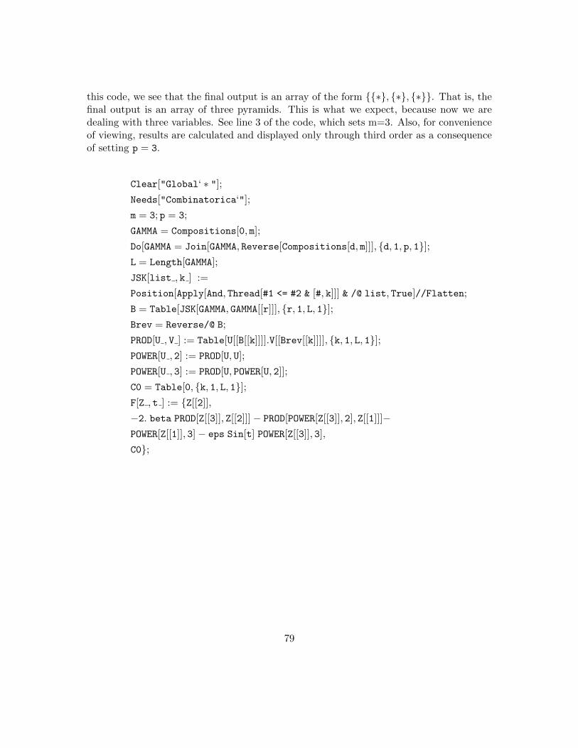
this code, we see that the final output is an array of the form ∗, ∗, ∗. That is, thefinal output is an array of three pyramids. This is what we expect, because now we aredealing with three variables. See line 3 of the code, which sets m=3. Also, for convenienceof viewing, results are calculated and displayed only through third order as a consequenceof setting p = 3.

Clear["Global‘ ∗ "];

Needs["Combinatorica‘"];

m = 3; p = 3;

GAMMA = Compositions[0, m];

Do[GAMMA = Join[GAMMA, Reverse[Compositions[d, m]]], d, 1, p, 1];L = Length[GAMMA];

JSK[list , k ] :=

Position[Apply[And, Thread[#1 <= #2 & [#, k]]] & /@ list, True]//Flatten;

B = Table[JSK[GAMMA, GAMMA[[r]]], r, 1, L, 1];Brev = Reverse/@ B;

PROD[U , V ] := Table[U[[B[[k]]]].V[[Brev[[k]]]], k, 1, L, 1];POWER[U , 2] := PROD[U, U];

POWER[U , 3] := PROD[U, POWER[U, 2]];

C0 = Table[0, k, 1, L, 1];F[Z , t ] := Z[[2]],

−2. beta PROD[Z[[3]], Z[[2]]]− PROD[POWER[Z[[3]], 2], Z[[1]]]−POWER[Z[[1]], 3]− eps Sin[t] POWER[Z[[3]], 3],

C0;

79

ns = 100;

t = 0;

h = (2Pi)/ns;

beta = .1; eps = 1.5;

zd0 = .3, .4, .5;C1 = Table[KroneckerDelta[k, 1], k, 1, L, 1];X[1] = Table[KroneckerDelta[k, 2], k, 1, L, 1];X[2] = Table[KroneckerDelta[k, 3], k, 1, L, 1];X[3] = Table[KroneckerDelta[k, 4], k, 1, L, 1];Zvar = zd0[[1]] C1 + X[1], zd0[[2]] C1 + X[2], zd0[[3]] C1 + X[3];RK4;

t

Zvar

2π

−0.0493158, 0.973942,−0.110494, 5.51271, 3.54684, 3.46678,

11.2762, 2.36463, 1.0985, 23.3332,−1.03541,−3.23761,−12.8064,

4.03421,−23.4342,−17.8967, 1.96148, 5.07403,−36.9009, 25.1379,0.439713, 1.05904, 0.427613, 3.3177, 0.0872459, 0.635397,−3.02822,

1.77416,−4.10115, 3.16981,−2.43002,−5.33643,−7.77038,−6.08476,

− 0.541465,−21.1672,−1.4091,−9.54326, 14.6334,−39.2312,0.5, 0, 0, 1, 0, 0, 0, 0, 0, 0, 0, 0, 0, 0, 0, 0, 0, 0, 0, 0

(7.120)

The first unusual fragments in the code are lines 12 and 13, which define functions thatimplement the calculation of second and third powers of pyramids. Recall Section 7.1.5.The first new fragment is line 14, which defines the pyramid C0 with the aid of the Tablecommand and an implied Do loop. As a result of executing this code, C0 is an array ofL zeroes. The next three lines, lines 15 through 18, define F, which specifies the rightsides of equations (6.12) through (6.14). See (6.15) through (6.18). The right side of F isof the form ∗, ∗, ∗, an array of three pyramids. By looking at (6.15) and recalling thereplacement rule, we see that the first pyramid should be Z[[2]],

z2 Z[[2]]. (7.121)

The second pyramid on the right side of F is more complicated. It arises by applying the

80

replacement rule to the right side of (6.16) to obtain the associated pyramid,

− 2βz3z2 − z23z1 − z3

1 − εz33 sin t

−2. beta PROD[Z[[3]], Z[[2]]]− PROD[POWER[Z[[3]], 2], Z[[1]]]−POWER[Z[[1]], 3]− eps Sin[t] POWER[Z[[3]], 3]. (7.122)

The third pyramid on the right side of F is simplicity itself. From (6.17) we see that thispyramid should be the result of applying the replacement rule to the number 0. Hence,this pyramid is C0,

0 C0 = 0, 0, · · · , 0. (7.123)

The remaining lines of the code require little comment. Line 20 sets the initial time to0, and line 21 defines h in such a way that the final value of t will be 2π. Line 22 establishesthe parameter values β = .1 and ε = 1.5, which are those for Figure 4. Line 23 specifiesthat the design initial condition is

z1(0) = zd01 = .3, z2(0) = zd0

2 = .4, z3(0) = zd03 = .5 = σ, (7.124)

and consequentlyω = 1/σ = 2. (7.125)

See (6.3). Also, it follows from (6.2) and (6.5) that

q(0) = ωQ(0) = ωz1(0) = (2)(.3) = .6, (7.126)

q′(0) = ω2Q(0) = ω2z2(0) = (22)(.4) = 1.6. (7.127)

Next, lines 24 through 28 specify that the expansion is to be carried out about the initialconditions (7.124). Finally, line 29 invokes the RK4 code given by (7.99). That is, as before,no modifications are required in the integration code.

A few more comments about the output are appropriate. Line 32 shows that the finaltime t is indeed 2π, as desired. The remaining output lines display the three pyramids thatspecify the final value of Zvar. From the first entry in each pyramid we see that

z1(2π) = −0.0493158, (7.128)

z2(2π) = 0.439713, (7.129)

z3(2π) = .5, (7.130)

when there are no deviations in the initial conditions. The remaining entries in the pyra-mids are the coefficients in the Taylor series that describe the changes in the final conditionsthat occur when changes are made in the initial conditions (including the parameter σ).We are, of course, particularly interested in the first two pyramids. The third pyramid hasentries only in the first place and the fourth place, and these entries are the same as those

81

in the third pyramid pyramid for Zvar at the start of the integration, namely those inzd0[3] C1 + X[3]. The fact that the third pyramid in Zvar remains constant is the expectedconsequence of (6.17).

We should also describe how the M8 employed in Section 6.2 was actually computed.It could have been computed by setting p = 8 in (7.120) and specifying a large number ofsteps ns to insure good accuracy. Of course, when p = 8, the pyramids are large. Therefore,one does not usually print them out, but rather writes them to files or sends them directlyto other programs for further use.

However, rather than using RK4 in (7.120), we replaced it with an adaptive 4-5th orderRunge-Kutta-Fehlberg routine that dynamically adjusts the time step h during the courseof integration to achieve a specified local accuracy, and we required that the error at eachstep be no larger than 10−12. Like the RK4 routine, the Runge-Kutta-Fehlberg routine,when implemented in Mathematica, has the property that it can integrate any number ofequations both in scalar variable and pyramid form without any changes in the code.10

7.4 Relation to the Complete Variational Equations

At this point it may not be obvious to the reader that the use of pyramids in integrationroutines to obtain Taylor expansions is the same as integrating the complete variationalequations. We now show that the integration of pyramid equations is equivalent to theforward integration of the complete variational equations. For simplicity, we will examinethe single variable case with no parameter dependence. The reader who has mastered thiscase should be able to generalize the results obtained to the general case.

In the single variable case with no parameter dependence (2.1) becomes

z = f(z, t). (7.131)

Let zd(t) be some design solution and introduce a deviation variable ζ by writing

z = zd + ζ. (7.132)

Then the equation of motion (7.131) takes the form

zd + ζ = f(zd + ζ, t). (7.133)

Also, the relations (2.4) and (2.5) take the form

f(zd + ζ, t) = f(zd, t) + g(zd, t, ζ) (7.134)

where g has an expansion of the form

g(zd, t, ζ) =∞∑j=1

gj(t)ζj . (7.135)

10A Mathematica version of this code is available from the first author upon request.

82

Finally, (2.6) and (2.7) becomezd = f(zd, t), (7.136)

ζ = g(zd, t, ζ) =∞∑j=1

gj(t)ζj , (7.137)

and (2.8) becomes

ζ =∞∑j=1

hj(t)(ζi)j . (7.138)

Insertion of (7.138) into both sides of (7.137) and equating like powers of ζi now yields theset of differential equations

hj′′(t) =

∞∑j=1

gj(t)U j′′

j (hs) with j, j′′ ≥ 1 (7.139)

where the (universal) functions U j′′

j (hs) are given by the relations ∞∑j′=1

hj′(ζi)

j′

j

=

∞∑j′′=1

U j′′

j (hs)(ζi)j′′ . (7.140)

The equations (7.136) and (7.139) are to be integrated from t = tin = t0 to t = tfin withthe initial conditions

zd(t0) = zd0, (7.141)

h1(t0) = 1, (7.142)

hj′′(t0) = 0 for j′′ > 1. (7.143)

Let us now consider the numerical integration of pyramids. Upon some reflection, we seethat the numerical integration of pyramids is equivalent to finding the numerical solutionto a differential equation with pyramid arguments. For example, in the single-variable case,let Zvar(t) be the pyramid appearing in the integration process. Then, its integration isequivalent to solving numerically the pyramid differential equation

(d/dt)Zvar(t) = F(Zvar, t). (7.144)

We now work out the consequences of this observation. By the inverse of the replace-ment rule, we may associate a Taylor series with the pyramid Zvar(t) by writing

Zvar(t) c0(t) +∑j≥1

cj(t)xj . (7.145)

83

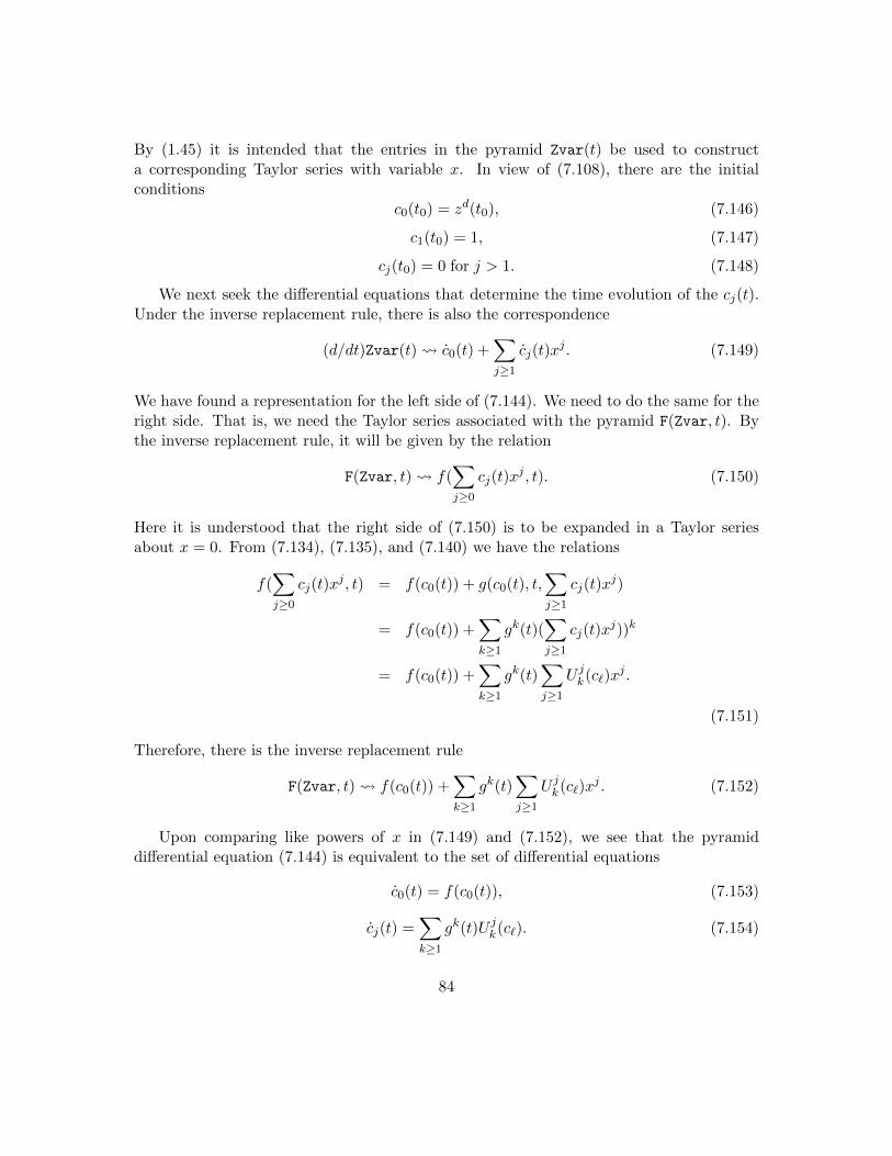
By (1.45) it is intended that the entries in the pyramid Zvar(t) be used to constructa corresponding Taylor series with variable x. In view of (7.108), there are the initialconditions

c0(t0) = zd(t0), (7.146)

c1(t0) = 1, (7.147)

cj(t0) = 0 for j > 1. (7.148)

We next seek the differential equations that determine the time evolution of the cj(t).Under the inverse replacement rule, there is also the correspondence

(d/dt)Zvar(t) c0(t) +∑j≥1

cj(t)xj . (7.149)

We have found a representation for the left side of (7.144). We need to do the same for theright side. That is, we need the Taylor series associated with the pyramid F(Zvar, t). Bythe inverse replacement rule, it will be given by the relation

F(Zvar, t) f(∑j≥0

cj(t)xj , t). (7.150)

Here it is understood that the right side of (7.150) is to be expanded in a Taylor seriesabout x = 0. From (7.134), (7.135), and (7.140) we have the relations

f(∑j≥0

cj(t)xj , t) = f(c0(t)) + g(c0(t), t,

∑j≥1

cj(t)xj)

= f(c0(t)) +∑k≥1

gk(t)(∑j≥1

cj(t)xj))k

= f(c0(t)) +∑k≥1

gk(t)∑j≥1

U jk(c`)x

j .

(7.151)

Therefore, there is the inverse replacement rule

F(Zvar, t) f(c0(t)) +∑k≥1

gk(t)∑j≥1

U jk(c`)x

j . (7.152)

Upon comparing like powers of x in (7.149) and (7.152), we see that the pyramiddifferential equation (7.144) is equivalent to the set of differential equations

c0(t) = f(c0(t)), (7.153)

cj(t) =∑k≥1

gk(t)U jk(c`). (7.154)

84

Finally, compare the initial conditions (7.141) through (7.143) with the initial conditions(7.146) through (7.148), and compare the differential equations (7.136) and (7.139) withthe differential equations (7.153) and (7.154). We conclude that that there must be therelations

c0(t) = zd(t), (7.155)

cj(t) = hj(t) for j ≥ 1. (7.156)

We have verified, in the single variable case, that the use of pyramids in integration routinesis equivalent to the solution of the complete variational equations using forward integration.As stated earlier, verification of the analogous m-variable result is left to the reader. Wealso observe the wonderful convenience that, when pyramid operations are implementedand employed, it is not necessary to explicitly work out the forcing terms gra(t) and thefunctions U r′′

r (hsn), nor is it necessary to set up the equations (3.6). All these complicationsare handled implicitly and automatically by the pyramid routines.

8 Concluding Summary

Poincare analyticity implies that transfer maps arising from ordinary differential equationscan be expanded as Taylor series in the initial conditions and also in whatever parametersmay be present. Section 2 showed that the determination of these expansions is equiva-lent to solving the complete variational equations, and Sections 3 and 4 showed that thecomplete variational equations can be solved either by forward or backward integration.Sections 5 and 6 applied this procedure for the Duffing stroboscopic map and found, re-markably, that an 8th order polynomial approximation to this map produced an infiniteperiod doubling cascade and apparent strange attractor that closely resembled those of theexact map. A final section described computer methods for automatically setting up andnumerically integrating the complete variational equations.

References

[1] J. Barrow-Green, Poincare and the Three Body Problem, American MathematicalSociety (1997).

[2] F. Browder, Edit., The Mathematical Heritage of Henri Poincare, Proceedings of Sym-posia in Pure Mathematics of the American Mathematical Society 39, Parts 1 and 2,American Mathematical Society (1983).

[3] H. Poincare, New Methods of Celestial Mechanics, Parts 1, 2, and 3. (Originally pub-lished as Les Methodes nouvelles de la Mechanique celeste.) American Institute ofPhysics History of Modern Physics and Astronomy, Volume 13, D. L. Goroff, Edit.,American Institute of Physics (1993).

85

[4] Francis J. Murray and Kenneth S. Miller, Existence Theorems for Ordinary DifferentialEquations, New York University Press and Interscience Publishing Co. (1954).

[5] The method of backward integration was discovered by F. Neri circa 1986.

[6] A. Dragt, Lie Methods for Nonlinear Dynamics with Applications to AcceleratorPhysics, (2011), available at http://www.physics.umd.edu/dsat/

[7] R. Neidinger, “Computing Multivariable Taylor Series to Arbitrary Order”, Proc. ofIntern. Conf. on Applied programming languages, San Antonio, pp. 134-144 (1995).

[8] Wolfram Research, Inc., Mathematica, Version 7.0, Champaign, IL (2008).

[9] D. Kalman and R. Lindell, “A recursive approach to multivariate automatic differen-tiation”, Optimization Methods and Software, Volume 6, Issue 3, pp. 161-192 (1995).

[10] M. Berz, “Differential algebraic description of beam dynamics to very high orders”,Particle Accelerators 24, p. 109 (1989).

86