Complementary variational principles with fractional derivatives

$: Complementary variational principles with fractional derivatives$
Acta Mech 223, 685–704 (2012)DOI 10.1007/s00707-011-0588-6

Teodor M. Atanackovic · Marko Janev · Stevan Pilipovic ·Dusan Zorica

Complementary variational principles with fractionalderivatives

Received: 29 April 2011 / Revised: 7 September 2011 / Published online: 20 December 2011© Springer-Verlag 2011

Abstract Complementary variational principles for a class of fractional boundary value problems areformulated. They are used for the error estimates of solutions for a general mechanical problems, first Painlevéequation also given in the form with fractional derivatives and in the task of image regularization.

1 Introduction

There exists a rich literature devoted to linear differential equations with non-integer derivatives, see [18,22,25,27,29,33] and the references therein. This is not the case for equations with left and right fractionalderivatives since such equations are much more complicated. The reason is that the Laplace transform, themain tool in solving fractional differential equations, cannot be used in this case, see [11,12,31]. However,the variational principles with the fractional derivatives in the Lagrangian function lead to Euler-Lagrangeequations with both left and right fractional derivatives (see [2–4,8,14,19]). Recall, fractional derivatives withrespect to time variable are used to model systems where the memory plays an important rule (see [24]),while fractional derivatives with respect to space variable model non-local phenomena (see [10,15]). It is,therefore, important to develop methods for solving such equations. Among such methods, we propose theRitz approach adjusted to fractional order equations, see [6,7,35] for integer order equations. In general, directmethods of the variational calculus provide an important tool for solving variational problems, especially ifthe complementary functionals are known. In this case, an easy error estimate procedure can be accomplished.

In this paper, we do not consider the existence theorems concerning the solutions to Euler-Lagrange equa-tions, i.e., minimizers of the fractional variational problems. We assume that solutions exist. Our intentionis to develop complementary variational principles for the fractional variational problems along the lines

T. M. AtanackovicDepartment of Mechanics, Faculty of Technical Sciences, University of Novi Sad,Trg D. Obradovica, 6, 21000 Novi Sad, SerbiaE-mail: [email protected]

M. Janev · D. Zorica (B)Mathematical Institute, Serbian Academy of Sciences and Arts, Beograd, Kneza Mihaila, 36, 11000 Beograd, SerbiaE-mail: [email protected]

M. JanevE-mail: [email protected]

S. PilipovicDepartment of Mathematics, Faculty of Natural Sciences and Mathematics,University of Novi Sad, Trg D. Obradovica, 4, 21000 Novi Sad, SerbiaE-mail: [email protected]

686 T. M. Atanackovic et al.

of [6,7,9,34]. In Sects. 3 and 4, we shall formulate theorems that give sufficient conditions for the existenceof the fractional complementary variational principles when the Lagrangians are of the form:

(i) L1(t, u, aDα

t u) = 1

2

(aDα

t u)2+Π (t, u) , u = (u1, . . . , un) is a vector function with the scalar argument

t, and aDαt u = (

aDαt u1, . . . , aDα

t un)

(see 4);(ii) L2(u, αgrad u) = Π(u)+ R(αgrad u), u is a scalar function with the vector argument x = (x1, . . . , xn)

and αgrad u = (αDx1u, . . . , αDxn u

)(see 7).

The practical aim of these theorems is to obtain an error estimate of an approximate solution to the Euler-Lagrange equations that correspond to the mentioned Lagrangians without knowing their exact solutions.These theorems will be proved in Sect. 5. The form of Lagrangian L1 is motivated by the applications inmechanics, as well as in the study of the first Painlevé equation, which we also formulate in terms of thefractional derivatives. Since we do not have the existence result for the solution to boundary value problemfor fractional and classical first Painlevé equation, we made the necessary assumption on their existence inorder to formulate the complementary principle and find the error estimate. The form of Lagrangian L2 ismotivated by the problems of the image regularization. Sections 3.1 and 3.2 are devoted to the application ofthe theory developed in Sect. 3 to general mechanical problems, where Lagrangian consist of two separateterms, representing kinetic and potential energy. These problems are also analyzed numerically, and the errorestimate is obtained. In Sect. 4.1, we use the theory presented in Sect. 4 for the image regularization task andgive the error estimate as well.

2 Notation

The left Riemann–Liouville fractional derivative of order α ∈ [n − 1, n) , n ∈ N, is defined (see [33]) as

aDαt f (t) =

(d

dt

)n

aIn−αt f (t) = 1

Γ (n − α)

(d

dt

)n t∫

a

(t − τ)n−α−1 f (τ ) dτ, t ∈ [a, b] . (1)

Similarly, the right Riemann–Liouville fractional derivative of order α ∈ [n − 1, n) , n ∈ N, is defined as

t Dαb f (t) =

(− d

dt

)n

t In−αb f (t) = 1

Γ (n − α)

(− d

dt

)n b∫

t

(τ − t)n−α−1 f (τ ) dτ, t ∈ [a, b] . (2)

Function f in (1) and (2) belongs to the set of n-times absolutely continuous function, denoted by ACn [a, b] ,i.e., f has n − 1 continuous derivatives, and the n-th derivative is an integrable function in [a, b] . We shallalso need the following integration by parts formula, see [33],

b∫

a

(aDα

t f (t))g (t) dt =

b∫

a

f (t)(

t Dαb g (t)

)dt. (3)

Here f ∈ aIαt (L p [a, b]) and g ∈ t Iαb (Lq [a, b]) , 1p + 1

q ≤ 1 + α, where aIαt (L p [a, b]) (and t Iαb (Lq [a, b]))

is the class of functions f that can be represented as f = aIαt ϕ(

f = t Iαb ϕ)

for some ϕ ∈ L p [a, b] , p ≥ 1.

Note that in the limit α → 1, (3) transforms into the classical formula, namely∫ b

a

( ddt f (t)

)g (t) dt =

[ f (t) g (t)]ba − ∫ b

a f (t)( d

dt g (t))

dt.

Let u (t) = (u1 (t) , . . . , un (t)) , t ∈ [a, b] , n ∈ N. We assume u ∈ (AC1 [a, b])n

and define the left andright Riemann–Liouville fractional derivative of u of order α ∈ (0, 1) as follows:

aDαt u := (

aDαt u1, . . . , aDα

t un), t D

αb u := (

t Dαb u1, . . . , t D

αb un

), (4)

where aDαt u j , respectively, t Dα

b u j , j ∈ {1, . . . , n} , are the left and right Riemann–Liouville fractional deriv-atives defined by (1) and (2).

Complementary variational principles 687

For the case of a function of a vector-valued argument, we shall need a generalization of a standard nabla

operator ∇ =(

∂∂x1

, . . . , ∂∂xn

). Let f ∈ C1 (Rn) . The (standard) gradient of a function is

grad f = ∇ f =(

∂ f

∂x1, . . . ,

∂ f

∂xn

).

Also in the case of the composition of functions f (x) = f (g (x)) , x ∈ Rn, g = (g1, . . . , gn) , we use

notation

gradg f = ∇g f =(

∂ f

∂g1, . . . ,

∂ f

∂gn

).

In order to “fractionalize” the Nabla operator ∇, we recall the Fourier transform of u ∈ L1 (Rn) ,

u (ξ) ≡ F [u (x)] (ξ) :=∫

Rn

u (x) e−iξ ·xdn x, ξ ∈ Rn,

where the dot in ξ · x denotes the scalar product. The fractional Sobolev space Hs (Rn) , s > 0, is defined by

Hs (R

n) = {u ∈ L2 (

Rn) : ‖u‖Hs(Rn) < ∞}

, where

‖u‖Hs(Rn) =⎛

⎝∫

Rn

(1 + |ξ |2)s ∣∣u (ξ)

∣∣2 dnξ

⎞

⎠

1/2

.(5)

The left and right fractional Nabla operators are

α∇ := (αDx1, . . . ,

αDxn

), ∇α := (

Dαx1

, . . . , Dαxn

), (6)

where

αDx j u := F−1 [(iξ j)α

u (ξ)], Dα

x ju := (−1)α αDx j u, j = 1, . . . , n.

We note that, like in the classical setting, we have the fractional gradients if the fractional Nabla operators (6)are applied to f ∈ Hs(Rn) as

αgrad f := α∇ f = (αDx1 f, . . . , αDxn f

), gradα f := ∇α f = (

Dαx1

f, . . . , Dαxn

f), (7)

and the fractional divergences of a vector function g = (g1, . . . , gn) , g ∈ (Hs (Rn))n , that are defined as

αdiv g := α∇ · g =n∑

j=1

αDx j g j , divα g := ∇α · g =n∑

j=1

Dαx j

g j .

Note that in the previous expressions, we used dot to denote the scalar product g · h := ∑nj=1 g j h j . Also, we

use the notation g2 ≡ g2 = g · g = ∑nj=1 g2

j . The integration by parts also holds, i.e., for f ∈ Hs(Rn) andg ∈ (Hs (Rn))n , s ≥ 1

∫

Rn

(αgrad f (x)

) · g (x) dn x =∫

Rn

f (x) divα g (x) dn x. (8)


3 Lagrangian depending on a vector function of scalar argument

We assume u = (u1, . . . , un) ∈ (AC2 [a, b])n

. Let us consider the Lagrangian

L(t, u, aDα

t u) = 1

2

(aDα

t u)2 + Π (t, u) , (9)

where(

aDαt u)2 = ∑n

j=1

(aDα

t u j)2

. We assume that [a, b] t �→ Π (t, ·) is a C1 mapping from [a, b] into

the space of function with the continuous derivatives up to order two, denoted by C2 (Rn) , i.e., Π (t, ·) :x �→ Π (t, x) , Π (t, ·) ∈ C2 (Rn) . We shall denote this space by C1

([a, b] ; C2 (Rn)

). In formulating the

Hamilton principle of least action, one is faced with the problem of finding a minimum of a functional

J (u) ≡ I(u, aDα

t u) =

b∫

a

L(t, u, aDα

t u)

dt =b∫

a

[1

2

(aDα

t u)2 + Π (t, u)

]dt, (10)

where u belongs to a space of admissible functions Un , defined as

Un ={

u : u ∈ (AC2 [a, b])n

, u satisfies prescribed boundary conditions}

.

We refer to [2,3,8] for the formulation of the Hamilton principle and Euler-Lagrange equations for the Lagrang-ian depending on a scalar function, as well as to [23] for the Lagrangian depending on a vector function.

In the sequel, we shall also refer to the principle of the least action as the primal variational principle.Requiring that (10) attains a minimum over Un , we obtain the Euler-Lagrange equations

t Dαb

(grad

aDαt u L

)+ gradu L = 0.

Since L has the form (9), we have(

gradaDα

t u L)

j= aDα

t u j , j ∈ {1, . . . , n} , and

t Dαb

(aDα

t u)+ gradu Π = 0. (11)

Each of the Euler-Lagrange equations can be written as a system of two equations with independent func-tions u and p. These equations are called the canonical (or the Hamilton) equations (for the case of a scalarfunction see [31]). In order to obtain the Hamilton equations, like in the classical case, we define the generalizedmomentum and the corresponding Hamiltonian as

p := gradaDα

t u L = aDαt u, (12)

H (t, u, p) := p · (aDαt u)− L

(t, u, aDα

t u) = 1

2p2 − Π (t, u) , (13)

where p ∈ Pn = (AC1[a, b])n at least, since aDαt u j = d

dt aI1−αt u j and aI1−α

t u j ∈ AC2 [a, b] , j = 1, . . . , n.

We write (10) in terms of the Hamiltonian as∫ b

a

[p · (aDα

t u)− H (t, u, p)

]dt, and use the integration by

parts formula (3) to obtain

I (u, p) =b∫

a

[(t D

αb p) · u − H (t, u, p)

]dt =

b∫

a

[(

t Dαb p) · u − 1

2p2 + Π (t, u)

]dt. (14)

Note that I is a functional with independent functions u and p. By requiring that I attains its minimum at(u, p) ∈ Un × Pn , we obtain the Hamilton equations

aDαt u = grad p H = p, t D

αb p = gradu H = −gradu Π. (15)

In order to formulate the dual functional, we pose the following condition that enables us to solve uniquelythe second Hamilton equation (15)2 with respect to u.

Condition 1 (a) Π ∈ C1([a, b] ; C2 (Rn)

) ;


(b) grad Π (t, ·) : Rn �→ D is a bijection of R

n to an open subset D of Rn for every t ∈ [a, b] ;

(c) det∣∣∣ ∂

2Π(t,x)∂xi ∂x j

∣∣∣ �= 0 for every t ∈ [a, b] and every x ∈ R

n .

If Condition 1 is satisfied, then there exists Φ : [a, b] × D �→ Rn, of class C1, such that

u (t) = Φ(t, t D

αb p (t)

), t ∈ [a, b] (16)

and

t Dαb p ≡ −gradΦ Π

(t, Φ

(t, t D

αb p))

, t ∈ [a, b] , (17)

i.e., the second Hamilton equation (15)2 is identically satisfied with Φ.Now, the dual functional G is obtained from (14) as ( p ∈ Pn)

G ( p) ≡ I (Φ (t, t D

αb p), p)

=b∫

a

[(t D

αb p) · Φ (

t, t Dαb p)− 1

2p2 + Π

(t, Φ

(t, t D

αb p))]

dt. (18)

Summarizing, we say that the complementary principle holds if for the primal functional J, (10), thereexists the dual functional G, (18), so that if J attains a minimum at a function u ∈ Un, then G attains amaximum at a function p ∈ Pn, where the connection between u and p is given by (12).

Theorem 1 Assume that Π satisfies Condition 1. Additionally, assume that there exists a constant c > 0, suchthat

n∑

i, j=1

∂2Π (t, x)

∂xi∂x jdxi dx j ≥ c (dx)2 , t ∈ [a, b] , x ∈ R

n . (19)

Then the complementary principle holds for the functionals (10) and (18), i.e., it holds

J (u) ≤ J (U) , G ( p) ≥ G (P) , (20)

where U = u + δu and P = p + δ p for u, U ∈ Un and p, P ∈ Pn . Moreover,

‖U − u‖L2[a,b] ≤√

2

c(J (U) − G (P)). (21)

The proof of Theorem is given in Sect. 5. For the estimates of type (21), where the Lagrangians in primaland dual functionals contain derivatives of integer order, see for example [6,9].

Remark 1 (i) Recall [16] that the necessary and sufficient condition for the positive definiteness of

V (t, dx) = ∑ni, j=1

∂2Π(t,x)∂xi ∂x j

dxi dx j is that there exists a continuous function V ∗ (dx) > 0, V ∗ (0) = 0,

such that V (t, dx) ≥ V ∗ (dx) for all (t, dx) ∈ [a, b] × Rn . Thus, (19) is the sufficient condition for

the positive definiteness.(ii) In certain cases, we can find k > 0, such that

∫ ba

(aDα

t δu)2 dt ≥ k

∫ ba (δu)2 dt. Then we have the sharper

form of (21):

‖U − u‖L2[a,b] ≤√

2

c + k(J (U) − G (P)). (22)

We shall show this in Proposition 1.


3.1 An example with the quadratic potential Π

In the following, we treat the Lagrangian (9) for the case of the one-dimensional function u = u (t) , t ∈ [0, 1]and the quadratic potential Π (t, u) = 1

2w (t) u2 (t) − q (t) u (t) , t ∈ [0, 1] , so that the Lagrangian (9) takesthe form

L(t, u, 0Dα

t u) = 1

2

(0Dα

t u)2 + 1

2wu2 − qu, (23)

where α ∈ (0, 1) , w ∈ C1 [0, 1] , mint∈[0,1] w (t) = w0 > 0, q ∈ C1 [0, 1] . We set the space of admissiblefunctions to be

U = {u : u ∈ C1 [0, 1] , u (0) = 0, 0Dα

t u (t)∣∣t=1 = 0

}.

According to [26], if u ∈ C1 [a, b] and α ∈ (0, 1) , then aDαt u ∈ Lr [a, b]

(t Dα

b u ∈ Lr [a, b])

for 1 ≤ r < 1α.

Since α ∈ (0, 1) , and u ∈ C1 [0, 1] , u (0) = 0, we have that 0Dαt u is continuous on [0, 1] . Note that (23)

represents the fractionalized Lagrangian considered in [6], p. 8.The Euler-Lagrange equation (11), subject to specified boundary conditions, reads

t Dα1

(0Dα

t u)+ wu − q = 0, u (0) = 0, 0Dα

t u (t)∣∣t=1 = 0, (24)

while the generalized momentum, according to (12), is p = 0Dαt u. Since the function Π satisfies Condition 1,

the second canonical equation (15)2 solved with respect to u yields

u = Φ(t, t D

α1 p) = − t Dα

1 p − q

w.

Therefore, the complementary functionals J and G, given by (10) and (18), respectively, become

J (u) =1∫

0

[1

2

(0Dα

t u)2 + 1

2wu2 − qu

]dt, (25)

G (p) = −1

2

1∫

0

[(t Dα

1 p − q)2

w+ p2

]

dt. (26)

The error estimate (21), given in Theorem 1, yields

‖U − u‖L2[0,1] ≤√

2

w0(J (U ) − G (P)), (27)

where U and P are approximate solutions to (24), since (19) yields

∂2Π (t, u)

∂u2 = w (t) ≥ w0, t ∈ [0, 1] .

Let us show that we can improve the error estimate (27) in the sense of Remark 1 (ii). Namely, we statethe following proposition.

Proposition 1 Let f ∈ L1 (0, 1) have an integrable fractional derivative 0Dαt f ∈ L∞ (0, 1) of order α ∈

( 12 , 1

), such that 0I1−α

t f (t)∣∣∣t=0

= 0. Let s1, s2 > 1, and s2 < 23−2α

. Then it holds

1∫

0

| f (τ )|2 dτ ≤ K

1∫

0

∣∣0Dαt f (τ )

∣∣2 dτ, (28)

where

K = σ 2σ

(Γ (α))2 (σ + α − 1)2σ (ρs1 + 1)1s1

, σ = 1

s2− 1

2, ρ = 2

(α + 1

s2

)− 3. (29)


Proof See Theorem 5.5, p. 57, from [5] and assume: p = 2, r = 2, ω1 = ω2 = 1, l = 1, μ1 = 0, r1 = 2.��

Therefore, by (28), (22) becomes

‖U − u‖L2[a,b] ≤√

2

w0 + 1K

(J (U ) − G (P)). (30)

Numerical analysis. In order to obtain an approximate solution to (24), we use the Ritz method. Thus, weassume

U (t) =N∑

i=1

ciUi (t) , t ∈ [0, 1] , (31)

where ci are arbitrary constants and Ui , i = 1, . . . , N , are trial functions satisfying boundary conditions(24)2,3. This leads to

0Dαt Ui (t) = Ui (0)

Γ (1 − α) tα+ 1

Γ (1 − α)

t∫

0

U ′i (τ )

(t − τ)αdτ

= 1

Γ (1 − α)

t∫

0

U ′i (τ )

(t − τ)αdτ.

Put

t∫

0

U ′i (τ )

(t − τ)αdτ = gi (t) , t ∈ [0, 1] , (32)

where gi , i = 1, . . . , N , are functions that will be given bellow. Boundary condition (24)3 implies gi (1) =0, i = 1, . . . , N . From [17], p. 572, we have that the solution of (32) reads

U ′i (t) = sin (απ)

π

d

dt

t∫

0

gi (τ )

(t − τ)1−αdτ, t ∈ [0, 1] , i = 1, . . . , N . (33)

Now, since gi (1) = 0, we chose gi in the form gi (t) = (1 − t)i , t ∈ [0, 1] , i = 1, . . . , N . Substituting thisin (33), we obtain, up to an arbitrary constants Ci

Ui (t) = Ci

t∫

0

(1 − τ)i

(t − τ)1−αdτ, t ∈ [0, 1] , i = 1, . . . , N .

We put Ci = 1, i = 1, . . . , N . The first three functions, defined for t ∈ [0, 1], are

U1 (t) = tα

α− tα+1

α (α + 1),

U2 (t) = tα

α− 2

tα+1

α (α + 1)+ 2

tα+2

α (α + 1) (α + 2),

U3 (t) = tα

α− 3

tα+1

α (α + 1)+ 6

tα+2

α (α + 1) (α + 2)− 6

tα+3

α (α + 1) (α + 2) (α + 3).


Let Pi = Γ (α) (1 − t)i , i = 1, . . . , N , and let ki , i = 1, . . . , N , be arbitrary constants. We shall find P inthe form

P (t) =N∑

i=1

ki Pi (t) , t ∈ [0, 1] . (34)

For the numerical purposes, we take w = w0 = q = 1, α = 0.6, and N = 9. By substituting (31) into(25) and minimizing with respect to ci , i = 1, . . . , 9, and by substituting (34) into (26) and maximizing withrespect to ki , i = 1, . . . , 9, we obtain

J (U ) = −0.176499, G (P) = −0.176850.

By applying Proposition 1, we obtain s2 < 23−2α

= 1.1111. We chose s1 = 2 and s2 = 1.1 so that from (29)we obtain K = 9.9771. The error estimate (30) yields

‖U − u‖L2[0,1] =√

2

w0 + 1K

(J (U ) − G (P)) = 0.0252692,

while from (27), we have

‖U − u‖L2[0,1] ≤ √2 (J (U ) − G (P)) = 0.0265053,

so that we improved the error estimate by 4.7%.Multiplying (24)1 by u, we obtain

[t D

α1

(0Dα

t u)]

u + u2 − u = 0. (35)

Integration of (35) and the use of (3) lead to

1∫

0

[(0Dα

t u)2

u + u2 − u]

dt = 2J (u) +1∫

0

u (t) dt = 0.

Therefore,

J (u) = −1

2

1∫

0

u (t) dt

and

−0.176499 ≤ −1

2

1∫

0

u (t) dt ≤ −0.176850.

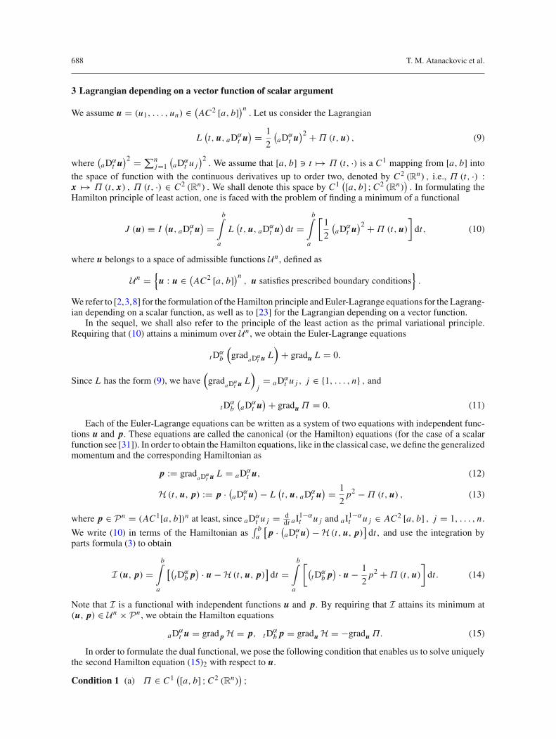
In Fig. 1, we present the plot of an approximate solution U for (24), obtained as described above.

3.2 Complementary principles for the fractional and classical first Painlevé equation

Our aim in this section is to formulate the complementary variational principles for the fractional and classicalfirst Painlevé equation. In the case of the fractional equation, we formulate the complementary principle on aspecific domain of admissible functions. In the case of the classical equation, we know the existence result forthe Cauchy problem (see [20]) and define the space of admissible functions in accordance with the initial datafor which solutions exist. In this way, we construct, in this set of admissible functions, a numerical solutionand give the error estimate. Our analysis opens several questions and indicates the possibility of the use of thecomplementary principles in both cases.

In both fractional and classical Painlevé equation, we set the space of admissible functions to be

U ={

u : u ∈ C2 [0, 1] , u (0) = 0, u (1) = 1, u (t) ≥√

t

6, t ∈ [0, 1]

}

. (36)


0.0 0.2 0.4 0.6 0.8 1.0t

0.1

0.2

0.3

0.4

0.5

U t

Fig. 1 Approximate solution U for (24)

The fractional first Painlevé equation. Consider the Lagrangian of the form (9)

L(t, u, 0Dα

t u) = 1

2

(0Dα

t u)2 + Π (t, u) , Π (t, u) = 2u3 − tu.

The Euler-Lagrange equation (11) corresponding to this Lagrangian is

t Dα1

(0Dα

t u (t)) = −6u2 (t) + t, t ∈ [0, 1] , (37)

where u ∈ U, given by (36). Actually, we can assume u ∈ AC2 ([0, 1]). We note that we do not if the solutionto (37) exists in U , and this is an open problem. If α = 1, then (37) is the first Painlevé equation on the finitetime interval t ∈ [0, 1] .

The primal functional (10) reads

J (u) =1∫

0

[1

2

(0Dα

t u)2 + 2u3 − tu

]dt. (38)

The generalized momentum (12) is p = 0Dαt u, so that the Hamiltonian (13) takes the form

H (t, u, p) = 1

2p2 − 2u3 + tu, t ∈ [0, 1] , u, p ∈ R.

The functional I, given by (14), reads

I (u, p) =1∫

0

[(

t Dα1 p)

u − 1

2p2 + 2u3 − tu

]dt =

1∫

0

[(

t Dα1 p)

u − 1

2p2 + 2u3 − tu

]dt. (39)

Canonical equations (also given by (15)) are obtained by the minimization of (39) as

0Dαt u = p, t D

α1 p = −6u2 + t, t ∈ [0, 1] , u, p ∈ R. (40)

Since Π satisfies Condition 1 and u ∈ U, the second canonical equation (40)2 solved with respect to u yields

u = Φ(t, t D

α1 p) =

√−t Dα1 p + t

6, t ∈ [0, 1] , p ∈ R. (41)

Therefore, the dual functional follows from (18), and it takes the form

G (p) = −1∫

0

[√6

9

(√−t Dα

1 p + t)3

+ 1

2p2

]

dt. (42)

Now, the error estimate follows from Theorem 1 and it is given by (21).


The classical first Painlevé equation. It is obtained from (37) as

u (t) = 6u2 − t, t ∈ [0, 1] , (43)

since limα→1 0Dαt u (t) = u (t) ≡ du(t)

dt , limα→1 t Dα1 u (t) = −u (t) and therefore limα→1 t Dα

1

(0Dα

t u (t)) =

−u (t) ≡ d2u(t)dt2 . We recall that the space of admissible functions U is given by (36).

Remark 2 We know [20, Lemma 1] that the Cauchy problem

u (t) = 6u2 − t, u (t)|t=0 = u0, u (t)|t=0 = v0, t > 0, (44)

has three sets of solutions denoted by A, B, and C. The set A consists of one-parameter family solutions thathave

√t as asymptotics as t → ∞. Set B consists of two-parameter family of solutions oscillating around the

asymptotics −√t as t → ∞. Set C is also a two-parameter family; it consists of solutions (as long as they

exist) that remain above the asymptotics√

t, or cross it from bellow (and therefore remain above). Also, from[20, Remark 4] we have that there exists γ > 0, such that all solutions to (44) with |u0| > γ and v0 = 0 in theset C blow up at some finite x0. Numerical experiments in [30, Table 1] show that the solutions to (44) belongto set B if initial data u0 and v0 have values in a certain domain.

Thus, having in mind the previous remark and since we consider the variational problem, we consider thesolutions belonging to either set A or set C (as long as the solution exists). Thus, we assume that initial andboundary data (36) are satisfied so that our solution coincides with the solution to the Cauchy problem (44)for suitably chosen initial data u0 and v0. This is the main hypothesis, and it will be tested in the subsequentnumerical analysis.

The primal functional, according to (38), reads

J (u) =1∫

0

[1

2u2 + 2u3 − tu

]dt. (45)

Canonical equations and the function Φ, by (40) and (41), are

u = p, p = 6u2 − t, u = Φ(t, t D

α1 p) =

√p + t

6. (46)

The dual functional is obtained from (42) as

G (p) = p (1) −1∫

0

[√6

9

(√p + t

)3 + 1

2p2

]

dt. (47)

We note that the first term in (47) is the consequence of integration by parts in (39), as described in Sect. 2,and the boundary conditions in (43)2,3.

Let U ≥ 0 and P be approximate solutions to (46)1,2. According to the complementary principle, we have

J (U ) − G (P) ≥ J (U ) − G (p) = J (U ) − J (u) ,

so that

J (U ) − G (P) ≥ 1

2

1∫

0

[(δu)2 + 12Ψ (δu)2] dt ≥ 1

2‖δu‖2

L2[0,1] , (48)

where Ψ = (1 − ε) u + εU > 0, ε ∈ (0, 1) . Let t∗ ∈ [0, 1] be such that

|M| := ‖δu‖L∞[0,1] = supt∈[0,1]

δu (t) .


Then, we have

M =t∗∫

0

δu (t) dt, i.e. |M| ≤t∗∫

0

|δu (t)| dt. (49)

On the other hand,

M = −1∫

t∗δu (t) dt, i.e. |M| ≤

1∫

t∗|δu (t)| dt. (50)

Thus, (49) and (50) imply

|M| ≤ 1

2

1∫

0

|δu (t)| dt.

By the Chauchy-Schwartz inequality, we have

|M| ≤ 1

2

⎛

⎝1∫

0

dt

⎞

⎠

1/2 ⎛

⎝1∫

0

|δu (t)|2 dt

⎞

⎠

1/2

, i.e. ‖δu‖L∞[0,1] ≤ 1

2‖δu‖L2[0,1] .

From the previous inequality and (48), if the solution to (43) exists, then we have

‖δu‖L∞[0,1] = ‖U − u‖L∞[0,1] ≤√

2

2

√J (U ) − G (P). (51)

Numerical analysis. We tested numerically the procedure outlined above. Thus, we assume

U (t) = c1tc2 + (1 − c1 − c4) tc3 + c4tc5, (52)

where c1, . . . , c5 are arbitrary constants. By substituting (52) into (45) and minimizing with respect to ci , i =1, . . . , 5, we obtain

U (t) = 0.858624 t5.3256 − 0.657 24 t5.3256 + 0.798615 t0.994154,

J (U ) = 0.609162.

Also, let

P (t) = d1 + d2td3 + d4td5, (53)

where d1, . . . , d5 are arbitrary constants. By substituting (53) into (47) and maximizing with respect to di , i =1, . . . , 5, we obtain

P (t) = 0.802055 + 0.504117 t3.96437 + 0.571215 t4.92265,

G (P) = 0.608744.

According to the formula for P, i.e., the approximate solution for u (see (46)1), we have P (0) = 0.802055.Since, u0 = 0 and (approximately) v0 = 0.802055, we see, according to [30, Table 1], that our solutionbelongs either to set A or to set C.

From (51), if the solution to (43) exists, we have

‖U − u‖L∞[0,1] ≤√

2

2

√J (U ) − G (P) = 0.014457.

In Fig. 2, we present the plot of an approximate solution U for (43), obtained as described above.


0.2 0.4 0.6 0.8 1.0t

0.2

0.4

0.6

0.8

1.0

U t

Fig. 2 Approximate solution U for (43)

4 Lagrangian depending on a scalar function of vector argument

We consider a scalar function u (x) = u (x1, . . . , xn) , such that u ∈ U = Hs+α (Rn) ∩ L∞ (Rn) , α > 0,s ≥ max {1, α} , where Hs is the Sobolev space defined in Sect. 2. This implies that u(α) = αgrad u ∈(Hs (Rn) ∩ L∞ (Rn))n . We consider the Lagrangian

L(u, u(α)) = Π(u) + R(u(α)), (54)

where Π ∈ C2 (R) satisfies Π ′′ (x) = d2Πdx2 ≥ c, c > 0, for every x ∈ R and R ∈ C∞ (Rn) satisfies

grad R (x)|x=0 = 0. This condition is motivated by the classical case, where R(u(α=1)) is the kinetic energyand it is equal to zero when all velocities (components of u(1)) are zero. This form of the Lagrangian is usedin the image denoising, which will be demonstrated by an example in Sect. 4.1. The primal functional has theform

J (u) ≡ I (u, u(α)) =∫

Rn

L(u, u(α))dn x =∫

Rn

(Π(u) + R(u(α))

)dn x. (55)

The Euler-Lagrange equation, obtained by the minimization of the primal functional J, is1

divα(gradu(α) L

)+ ∂L

∂u= 0, i.e.

Π ′ + divα(gradu(α) R

) = 0, or Π ′(u) +n∑

j=1

Dαx j

∂ R(αDx1u, . . . , αDxn u

)

∂ αDx j u= 0.

(56)

The generalized momentum is defined by

p := gradu(α) L = gradu(α) R. (57)

In order to show that p ∈ Pn = (Hs (Rn))n , s ≥ max {1, α} , we use:

Theorem 2 ([32], Theorem 2, p. 368) Let G ∈ C∞ (Rn) and let G (0) = 0. Suppose s ≥ 1 and σp < s <

m ∈ N, where σp = n · max{

0, 1p − 1

}. Then there exists a constant c, such that

‖G ( f1, . . . , fn)‖Fsp,q (R) ≤ c · max

j∈[1,n]

(∥∥ f j

∥∥

Fsp,q (R)

)· max

j∈[1,n]

(1 + ∥

∥ f j∥∥m−1

L∞(R)

),

holds for all ( f1, . . . , fn) ∈(

Fsp,q (R) ∩ L∞ (R)

)n.

1 The procedure of deriving (56) is standard one (see [2]) and it is omitted, although we have not seen equation of the type(56) before.


According to [32], (vi) on p. 13, Proposition (vii) on p. 14 and (5), we have that Hs = Hs2 = Fs

2,2, so

that σ2 = n · max{0,− 1

2

} = 0. We also have that p j = ∂ R(αDx1 u,...,αDxn u

)

∂ αDx j u is such that p j ∈ Hs (Rn) ∩L∞ (Rn) , j = 1, . . . , n, since

(αDx1u, . . . , αDxn u

) ∈ (Hs (Rn) ∩ L∞ (Rn))n ,∂ R(αDx1 u,...,αDxn u

)

∂ αDx j u ∈C∞ (Rn) and ∂ R(x1,...,xn)

∂x j

∣∣∣(x1,...,xn)=(0,...,0)

= 0.

Note that we assumed s ≥ max {1, α} because in (56), we have divα(gradu(α) R

) = divα p.We define the Hamiltonian as

H (u, p) := p · u(α) − L(u, u(α)) = p · u(α) − Π(u) − R(u(α)). (58)

The Hamiltonian depends on both canonical variables (u, p); hence, we use (57) and the following conditionin order to obtain u(α) as a function of p.

Condition 2 (a) R ∈ C∞ (Rn) ;(b) grad R : R

n �→ D is a bijection on open set D ⊂ Rn;

(c) det∣∣∣ ∂

2 R(x)∂xi ∂x j

∣∣∣ �= 0 for every x ∈ R

n .

Then, by the implicit function theorem, there exists ϒ : D �→ Rn of class (C∞)n , such that (57) can be

inverted and solved for u(α), i.e.,

u(α) = ϒ ( p) .

Therefore, (58) becomes

H (u, p) = p · ϒ ( p) − Π(u) − R(ϒ ( p)). (59)

We write the Lagrangian in (55) by using (58), i.e., we express the Lagrangian in terms of the Hamiltonian, sothat

I (u, u(α)) =∫

Rn

[p · u(α) − H (u, p)

]dn x.

Next we use the integration by parts formula (8) to obtain

I (u, p) =∫

Rn

[u divα p − H (u, p)

]dn x

=∫

Rn

[u divα p − p · ϒ ( p) + Π(u) + R(ϒ ( p))

]dn x. (60)

We treat (60) as a variational problem with independent functions u and p. By minimizing (60) with respectto (u, p) ∈ U × Pn , we obtain the Hamilton equations

u(α) = grad p H = ϒ ( p) , divα p = ∂H∂u

= −Π ′. (61)

In order to formulate the dual functional, we solve the second Hamilton equation (61)2 with respect to u. SinceΠ ∈ C2 (R) satisfies Π ′′ (x) ≥ c, c > 0, for every x ∈ R, there exists θ : R �→ R of class C1, such that (61)2can be inverted and solved for u, i.e.,

u = θ(divα p

). (62)

Finally, by (60) and (62), we obtain the dual functional as

G ( p) =∫

Rn

[θ(divα p

)divα p − p · ϒ ( p) + Π

(θ(divα p

))+ R(ϒ ( p))]

dn x. (63)

We formulate the following theorem, which we prove in Sect. 5.


Theorem 3 Assume that Π ∈ C2 (R) satisfies Π ′′ (x) ≥ c, c > 0, for every x ∈ R. Also assume thatR ∈ C∞ (Rn) satisfies grad R (x)|x=0 = 0 and Condition 2. Additionally, assume

n∑

i, j=1

∂2 R (x)

∂xi∂x jdxi dx j ≥ 0, x ∈ R

n . (64)

Then the complementary principle holds for the functionals (55) and (63), i.e., it holds

J (u) ≤ J (U ) , G ( p) ≥ G (P) , (65)

where U = u + δu and P = p + δ p for u, U ∈ U and p, P ∈ Pn . Moreover,

‖U − u‖L2(Rn) ≤√

2

c(J (U ) − G(P)). (66)

Again, the corresponding results for the Lagrangians containing integer order derivatives are given in [6].

4.1 Example in the image regularization

In this section, as an example of the general theory presented in Sect. 4, we shall specify the Lagrangian, given by(54), in the form that is intensively used the image denoising and regularization tasks (see [1,13,28]). Namely,in the Lagrangian (54) we chose Π (u) = 1

2λ(u −u0)

2, u0 ∈ Hs+α(R2), α > 0, s ≥ max {1, α} , λ > 0, and

R(u(α)) = √1 + (u(α))2, u(α) = αgrad u. This form of the function R is called the “minimal surface” edge

stopping function, see [1]. Therefore, the Lagrangian takes the form

L(u, u(α)) = 1

2λ(u − u0)

2 +√

1 + (u(α))2, u ∈ Hs+α(R2).

The primal functional (55) becomes

J (u) =∫

R2

[1

2λ(u − u0)

2 +√

1 + (u(α))2

]d2x, (67)

while the Euler-Lagrange equation, calculated by (56), is

divα u(α)

√1 + (u(α))2

+ u − u0

λ= 0.

The generalized momentum p ∈ (Hs(R

2))2

, given by (57), becomes

p := u(α)

√1 + (u(α))2

. (68)

Since R(x) = √1 + x2 satisfies Condition 2, we have that (68) can be solved with respect to u(α) as

u(α) = ϒ ( p) = p√

1 − p2. (69)

Note that from (69), it follows that p2 < 1. The Hamiltonian (59) takes the form

H (u, p) := − 1

2λ(u − u0)

2 −√

1 − p2,

while the canonical equations, given by (61), are

u(α) = p√

1 − p2, divα p = u0 − u

λ. (70)


Since Π (u) = 12λ

(u − u0)2 satisfies Π ′′ (u) = 1

λ= c ≥ 0, we have that the second canonical equation (70)2

can be solved with respect to u as

u = θ(divα p

) = u0 − λ divα p. (71)

The dual functional, according to (63), with (69) and (71), reads

G ( p) =∫

R2

[u0 divα p − 1

2λ(divα p

)2 +√

1 − p2

]d2x. (72)

According to Theorem 3, the primal functional (67) attains its minimum, while the dual functional (72)attains its maximum. Thus, by (66) we have

‖δu‖L2(Rn) ≤ √2λ (J (U ) − G(P)), (73)

since (64) is also satisfied. In [21], we calculate u by a numerical approach and obtain an approximate solutionfor which we use (73) in order to achieve the required precision of u.

5 Proofs of Theorems 1 and 3

In this section, we prove Theorems 1 and 3. Note that the assumptions of Sect. 3, respectively, Sect. 4, implythe existence of the functionals J and G, given in the form (10) and (18), respectively, (55) and (63).

Proof of Theorem 1 By the Taylor expansion formula for Π and U = u + δu, we have

J (U) − J (u) =b∫

a

[1

2

((aDα

t U)2 − (

aDαt u)2)+ Π (t, U) − Π (t, u)

]dt

=b∫

a

[(aDα

t u) · (aDα

t δu)+ δu · gradu Π (t, u)

]dt

+1

2

b∫

a

[(aDα

t δu)2 + δu · ([δu · ∇u] gradu Π (t, u)

)]

u=ξdt

= 1

2

b∫

a

⎡

⎣(aDαt δu

)2 +n∑

i, j=1

∂2Π (t, u)

∂ui∂u j(δui )

(δu j

)⎤

⎦

u=ξ

dt

≥ c

2

b∫

a

(δu)2 dt = c

2‖δu‖2

L2[a,b] , (74)

where ξ = u + η (U − u) , η ∈ (0, 1) . In obtaining (74), we used integration by parts formula (3) in order touse the Euler-Lagrange equations (11). We also used (19). Therefore, J (U) ≥ J (u) .

Further, consider G ( p) and assume that p ∈ Pn is a solution to (15). Let P = p + δ p be an arbitraryelement of Pn . We use the Taylor expansion formula for Π and Φ and consider the difference

G (P) − G ( p)

=b∫

a

[(

t Dαb P) · Φ

(t, t D

αb P)− (

t Dαb p) · Φ (

t, t Dαb p)

−1

2

[P2 − p2]+ Π

(t, Φ

(t, t D

αb P))− Π

(t, Φ

(t, t D

αb p)) ]

dt


=b∫

a

[ (t D

αb δ p

) · Φ (t, t D

αb p)− p · δ p

+([(

t Dαb δ p

) · ∇t Dαb p

]Φ(t, t D

αb p)) · ((t Dα

b p)+ gradΦ Π

(t, Φ

(t, t D

αb p)))]

dt

+1

2

b∫

a

[2(

t Dαb δ p

) ·([(

t Dαb δ p

) · ∇t Dαb p

]Φ(t, t D

αb p))− (δ p)2

+([(

t Dαb δ p

) · ∇t Dαb p

]2Φ(t, t D

αb p))

· ((t Dαb p)+ gradΦ Π

(t, Φ

(t, t D

αb p)))

+([(

t Dαb δ p

) · ∇t Dαb p

]Φ(t, t D

αb p))

×[ [([(

t Dαb δ p

) · ∇t Dαb p

]Φ(t, t D

αb p)) · ∇Φ

]gradΦ Π

(t, Φ

(t, t D

αb p))] ]

p=ζ

dt,

where ζ = p + η (P − p) , η ∈ (0, 1) . By (17), we have(

t Dαb p)+ gradΦ Π

(t, Φ

(t, t D

αb p)) = 0,

while, according to (3), (16), and (15)1, we have

b∫

a

[(t D

αb δ p

) · Φ(t, t D

αb p)− p · δ p

] =b∫

a

[aDα

t Φ(t, t D

αb p)− p

] · δ p = 0.

Thus, we obtain

G (P) − G ( p) = −1

2

b∫

a

[(δ p)2 − (2w1 + w2)

]p=ζ

dt, (75)

where

w1 := (t D

αb δ p

) ·([(

t Dαb δ p

) · ∇t Dαb p

]Φ(t, t D

αb p))

=n∑

i, j=1

∂Φ j(t, t Dα

b p)

∂ t Dαb pi

δ(

t Dαb pi

)δ(

t Dαb p j

), (76)

w2 :=([(

t Dαb δ p

) · ∇t Dαb p

]Φ(t, t D

αb p))

×([([(

t Dαb δ p

) · ∇t Dαb p

]Φ(t, t D

αb p)) · ∇Φ

]gradΦ Π

(t, Φ

(t, t D

αb p)))

=n∑

i, j,k,l=1

∂2Π(t, Φ

(t, t Dα

b p))

∂Φi∂Φ j

∂Φi(t, t Dα

b p)

∂ t Dαb pk

∂Φ j(t, t Dα

b p)

∂ t Dαb pl

δ(

t Dαb pk

)δ(

t Dαb pl

).

(77)

Let us write (17) as

t Dαb p j = −∂Π

(t, Φ

(t, t Dα

b p))

∂Φ j, j = 1, . . . , n,

and differentiate it with respect to t Dαb pk . Then we obtain

δ j,k = −n∑

i=1

∂2Π(t, Φ

(t, t Dα

b p))

∂Φ j∂Φi

∂Φi(t, t Dα

b p)

∂ t Dαb pk

, (78)


where δ j,k denotes the Kronecker delta. According to (76) and by the use of (78) in (77), we have

w2 = −n∑

k,l=1

∂Φk(t, t Dα

b p)

∂ t Dαb pl

δ(

t Dαb pk

)δ(

t Dαb pl

) = −w1.

Now, (75) becomes

G (P) − G ( p) = −1

2

b∫

a

[(δ p)2 +

n∑

i, j,k,l=1

∂2Π(t, Φ

(t, t Dα

b p))

∂Φi∂Φ j

×∂Φi(t, t Dα

b p)

∂ t Dαb pk

∂Φ j(t, t Dα

b p)

∂ t Dαb pl

δ(

t Dαb pk

)δ(

t Dαb pl

) ]

p=ζ

dt ≥ 0.

We conclude that G ( p) ≥ G (P) .Let U and P be two approximate solutions to (15). Since J (U) ≥ J (u) and G ( p) ≥ G (P) , we have

that (20) holds. Moreover,

J (U) − G (P) ≥ J (U) − G ( p) = J (U) − J (u) ,

so that by (74) it holds

J (U) − G (P) ≥ c

2‖δu‖2

L2[a,b] .

��Proof of Theorem 3 By the use of the Taylor formula, U = u + δu and αgrad (δu) = δ (αgrad u) = δu(α),we have

J (U ) − J (u)

=∫

Rn

[Π(U ) − Π(u) + R(U (α)) + R(u(α))

]dn x

=∫

Rn

[Π ′(u)δu + δu(α) · gradu(α) R(u(α))

]dn x

+1

2

∫

Rn

[Π ′′(u)(δu)2 + δu(α) ·

([δu(α) · ∇u(α)

]gradu(α) R(u(α))

)]

u=ξdn x

= 1

2

∫

Rn

⎡

⎣Π ′′(u)(δu)2 +n∑

i, j=1

∂2 R(u(α))

∂(αDxi u

)∂(αDx j u

)δ(αDxi u

)δ(αDx j u

)⎤

⎦

u=ξ

dn x

≥ c

2

∫

Rn

(δu)2dn x = c

2‖δu‖2

L2(Rn), (79)

where ξ = u + η (U − u) , η ∈ (0, 1) . In obtaining (79), we used integration by parts formula (8) in order touse the Euler-Lagrange equations (56). We also used (64). Therefore, J (U ) ≥ J (u) .

Now consider (63). It follows

G(P) − G( p) := Δ1 + Δ2, (80)

where

Δ1 :=∫

Rn

[P(α)θ(P(α)) − p(α)θ(p(α)) + Π(θ(P(α))) − Π(θ(p(α)))

]dn x, (81)

Δ2 :=∫

Rn

[R (ϒ (P)) − R (ϒ ( p)) − P · ϒ(P) + p · ϒ( p)

]dn x. (82)


In (81), we used the notation P(α) = divα P and p(α) = divα p. By the use of the Taylor formula, andP = p + δ p, (81) becomes

Δ1 =∫

Rn

[θ(p(α)) + dθ(p(α))

d p(α)

(p(α) + dΠ(θ)

dθ

)]δp(α)dn x

+1

2

∫

Rn

[(

2dθ(p(α))

d p(α)+ d2Π(θ)

dθ2

(dθ(p(α))

d p(α)

)2

+ d2θ(p(α))

d(p(α))2

(p(α) + dΠ(θ)

dθ

))(δp(α))2

]

p(α)=divα ξ

dn x, (83)

where ξ = p + ε(P − p), for some ε ∈ (0, 1). According to (61)2, we have

p(α) + dΠ(θ)

dθ= 0.

Having in mind that θ = θ(p(α)), see (62), differentiation of the previous expression with respect to p(α)

yields

1 + d2Π(θ)

dθ2

dθ(p(α))

d p(α)= 0,

so that (83) becomes

Δ1 =∫

Rn

θ(p(α))δp(α)dn x − 1

2

∫

Rn

[(d2Π(θ)

dθ2

)−1

(δp(α))2

]

p(α)=divα ξ

dn x. (84)

Now, by the use of the Taylor formula in (82), we obtain

Δ2 =∫

Rn

[ [(δ p · ∇ p

)ϒ( p)

] · (gradϒ R (ϒ) − p)− ϒ( p) · δ p

]dn x

+1

2

∫

Rn

[ [(δ p · ∇ p

)2ϒ( p)

]· (gradϒ R (ϒ) − p

)− 2δ p · [(δ p · ∇ p)ϒ( p)

]

+ [(δ p · ∇ p

)ϒ( p)

] · [([(δ p · ∇ p)ϒ( p)

] · ∇ϒ

)gradϒ R (ϒ)

] ]

p=ξ

dn x, (85)

where ξ = p + ε(P − p), for some ε ∈ (0, 1). According to (57) and (61), we have

p = gradϒ R (ϒ) , (86)

so that (85) yields

Δ2 = −∫

Rn

ϒ( p) · δ p dn x − 1

2

∫

Rn

[2q1 − q2] p=ξ dn x, (87)

where

q1 := δ p · [(δ p · ∇ p)ϒ( p)

] =n∑

k,l=1

∂ϒk

∂plδpkδpl , (88)

q2 := [(δ p · ∇ p

)ϒ( p)

] · [([(δ p · ∇ p)ϒ( p)

] · ∇ϒ

)gradϒ R (ϒ)

]

=n∑

i, j,k,l=1

∂2 R (ϒ)

∂ϒi ∂ϒ j

∂ϒi

∂pk

∂ϒ j

∂plδpkδpl . (89)


We write (86) as

p j = ∂ R (ϒ ( p))

∂ϒ j, j = 1, . . . , n,

and differentiate it with respect to pk . Then we obtain

δ j,k =n∑

i=1

∂2 R (ϒ ( p))

∂ϒ j ∂ϒi

∂ϒi

∂pk. (90)

According to (88) and by the use of (90) in (89), we have

q2 =n∑

k,l=1

∂ϒk

∂plδpkδpl = q1.

Now, (87) becomes

Δ2 = −∫

Rn

ϒ( p) · δ p dn x − 1

2

∫

Rn

⎡

⎣n∑

i, j,k,l=1

∂2 R (ϒ)

∂ϒi ∂ϒ j

∂ϒi

∂pk

∂ϒ j

∂plδpkδpl

⎤

⎦

p=ξ

dn x.

Using the previous expression and (84) in (80), we obtain

G(P) − G( p) =∫

Rn

[θ(divα p)

(divα δ p

)− ϒ( p) · δ p]

dn x

−1

2

∫

Rn

[(d2Π(θ)

dθ2

)−1 (divα δ p

)2

+n∑

i, j,k,l=1

∂2 R (ϒ)

∂ϒi ∂ϒ j

∂ϒi

∂pk

∂ϒ j

∂plδpkδpl

]

p=ξ

dn x. (91)

By (8), (61)1, (62), and u(α) = αgrad u, we have∫

Rn

[θ(divα p

) (divα δ p

)− ϒ ( p) · δ p]

dn x

=∫

Rn

[αgrad

(θ(divα p

))− ϒ ( p)] · δ p dn x = 0,

so that (91) becomes

G(P) − G( p) = −1

2

∫

Rn

[(d2Π(θ)

dθ2

)−1 (divα δ p

)2

+n∑

i, j,k,l=1

∂2 R (ϒ)

∂ϒi ∂ϒ j

∂ϒi

∂pk

∂ϒ j

∂plδpkδpl

]

p=ξ

dn x ≤ 0.

We conclude that G ( p) ≥ G (P) .Let U and P be two approximate solutions to (61). Since J (U ) ≥ J (u) and G ( p) ≥ G (P) , we have

that (65) holds. Moreover, we have

J (U ) − G (P) ≥ J (U ) − G ( p) = J (U ) − J (u) .

Thus, by (79),

J (U ) − G (P) ≥ c

2‖δu‖2

L2(Rn).

��


Acknowledgments This research was supported by projects 174005 (T.M.A. and D.Z.), TR32035 (M.J.), and 174024, III44006(S.P.) of the Serbian Ministry of Science.

References

1. Aubert, G., Kornprobst, P.: Mathematical Problems in Image Processing, Partial Differential Equations and the Calculus ofVariation. Springer Science + Business media, LLC, New York (2006)

2. Agrawal, O.P.: Formulation of Euler-Lagrange equations for fractional variational problems. J. Math. Anal. Appl. 272,368–379 (2002)

3. Agrawal, O.P.: Fractional variational calculus and the transversality conditions. J. Phys. A Math. Gen. 39, 10375–10384 (2006)

4. Agrawal, O.P., Muslih, S.I., Baleanu, D.: Generalized variational calculus in terms of multi-parameters fractional deriva-tives. Commun. Nonlinear Sci. Numer. Simulat. 16, 4756–4767 (2011)

5. Anastassiou, G.A.: Fractional Differentiation Inequalities. Springer Science + Business Media, LLC, New York (2009)6. Arthurs, A.M.: Complementary Variational Principles. Clarendon Press, Oxford (1980)7. Arthurs, A.M.: Dual extremum principles and error bounds for a class of boundary value problems. J. Math. Anal. Appl.

41, 781–795 (1973)8. Atanackovic, T.M., Konjik, S., Pilipovic, S.: Variational problems with fractional derivatives: Euler-Lagrange equations.

J. Phys. A Math. Theor. 41, 095201 (12 p) (2008)9. Atanackovic, T.M., Djukic, Dj.S.: An extremum variational principle for a class of boundary value problems. J. Math. Anal.

Appl. 93, 344–362 (1983)10. Atanackovic, T.M., Stankovic, B.: Generalized wave equation in nonlocal elasticity. Acta Mech. 208, 1–10 (2009)11. Atanackovic, T.M., Stankovic, B.: On a class of differential equations with left and right fractional derivatives. Z. Angew.

Math. Mech. 87, 537–546 (2007)12. Atanackovic, T.M., Stankovic, B.: On a differential equation with left and right fractional derivatives. Fract. Calc. Appl. Anal.

10, 139–150 (2007)13. Bai, J., Feng, X.C.: Fractional order anisotropic diffusion for image denoising. IEEE T. Image Process. 16, 2492–2502 (2007)14. Baleanu, D.: Fractional variational principles in action. Phys. Scr. T 136, 014006–014011 (2009)15. Carpinteri, A., Cornetti, P., Sapora, A.: A fractional calculus approach to nonlocal elasticity. Eur. Phys. J. Special Top.

193, 193–204 (2011)16. Demidovic, B.P.: Lectures on Mathematical Theory of Stability. Nauka, Moscow (1967) (in Russian)17. Gahov, F.D.: Boundary Value Problems. Nauka, Moscow (1977) (in Russian)18. Gorenflo, R., Vessella, S.: Abel Integral Equations. Lecture Notes in Mathematics 1461. Springer, Berlin (1991)19. Herzallah, M.A.E., Baleanu, D.: Fractional-order Euler-Lagrange equations and formulation of Hamiltonian equations.

Nonlinear Dyn. 58, 385–391 (2009)20. Holmes, P., Spence, D.: On a Painlevé-type boundary-value problem. Q. J. Mech. Appl. Math. 37, 525–538 (1984)21. Janev, M., Atanackovic, T., Pilipovic, S., Obradovic, R.: Image denoising by a direct variational minimization. EURASIP

J. Adv. Sig. Pr. 2011:8 (2011)22. Kilbas, A.A., Srivastava, H.M., Trujillo, J.J.: Theory and Applications of Fractional Differential Equations. Elsevier,

Amsterdam (2006)23. Klimek, M.: On Solutions of Linear Fractional Differential Equations of a Variational Type. Czestochowa University of

Technology, Czestochowa (2009)24. Mainardi, F.: Fractional Calculus and Waves in Linear Viscoelasticity. Imperial College Press, London (2010)25. Miller, K.S., Ross, B.: An Introduction to the Fractional Calculus and Fractional Differential Equations. Wiley, New

York (1993)26. Mishura, Y.S.: Stochastic Calculus for Fractional Brownian Motion and Related Processes. Springer, Berlin (2008)27. Oldham, K.B., Spanier, J.: The Fractional Calculus. Academic Press, New York (1974)28. Perona, P., Malik, J.: Scale-space and edge detection using anisotropic diffusion. IEEE T. Pattern Anal. 12, 629–639 (1990)29. Podlubny, I.: Fractional Differential Equations. Academic Press, San Diego (1999)30. Qin, HZ., Lu, YM.: A note on an open problem about the first Painlevé equation. Acta Math. Appl. Sin-E. 24, 203–210 (2008)31. Rabei, E.M., Nawafleh, K.I., Hijjawi, R.S., Muslih, S.I., Baleanu, D.: The Hamilton formalism with fractional derivatives.

J. Math. Anal. Appl. 327, 891–897 (2007)32. Runst, T., Sickel, W.: Sobolev Spaces of Fractional Order, Nemytskij Operators, and Nonlinear Partial Differential

Equations. Walter de Gruyter & Co, Berlin (1996)33. Samko, S.G., Kilbas, A.A., Marichev, I.I.: Fractional Integrals and Derivatives. Gordon and Breach, Amsterdam (1993)34. Sewell, M.J.: Maximum and Minimum Principles. Cambridge University Press, Cambridge (1987)35. Vujanovic, B.D., Jones, S.E.: Variational Methods in Nonconservative Phenomena. Academic press, London (1989)

Complementary variational principles with fractional derivatives

Documents

Transcript of Complementary variational principles with fractional derivatives