Variational Segmentation of Elongated Volumetric Structures∗

Christian Reinbacher, Thomas Pock, Christian Bauer, Horst BischofInstitute for Computer Graphics and Vision

Graz University of Technology, Austriareinbacher,pock,cbauer,bischof@icg.tugraz.at

Abstract

We present an interactive approach for segmenting thinvolumetric structures. The proposed segmentation modelis based on an anisotropic weighted Total Variation energywith a global volumetric constraint and is minimized us-ing an efficient numerical approach and a convex relax-ation. The algorithm is globally optimal w.r.t. the relaxedproblem for any volumetric constraint. The binary solu-tion of the relaxed problem equals the globally optimal so-lution of the original problem. Implemented on today’suser-programmable graphics cards, it allows real-time userinteraction. The method is applied to and evaluated onthe task of articular cartilage segmentation of human kneejoints and segmentation of tubular structures like liver ves-sels and airway trees.

1. IntroductionMedical volumetric images are three-dimensional im-

ages which contain several anatomical structures. Depend-ing on the imaging method, different structures can be visu-alized. These images are usually inspected by radiologists.For diagnosis and therapeutic interventional planning, thefirst step usually is an accurate segmentation of one ob-ject. In many applications (e.g. cartilage) the segmenta-tion of very thin and elongated objects is necessary whichposes additional difficulties. Current research is focusing onspeeding up this lengthy process by providing either fully-automatic or semi-automatic segmentation methods. Auto-matic methods like [12, 13, 14, 15] have proven very usefulfor medical studies where a large amount of data has to beprocessed. However, in some cases the ability to control andcorrect segmentation results is necessary in order to gain therequired accuracy [19]. In this case the goal is to minimizethe required interaction time.

1This work was supported by the Austrian Science Fund (FWF) underthe doctoral program Confluence of Vision and Graphics W1209 and theAustrian Research Promotion Agency (FFG) under the project SILHOU-ETTE (825843).

(a) Geodesic Active Con-tour model

(b) Proposed segmenta-tion model

Figure 1: Segmentation results for articular cartilage of a humanknee joint. (a) is obtained using a standard GAC segmentationmodel, (b) is obtained by incorporating edge direction informationinto the segmentation model.

Modern imaging technologies such as Magnetic Reso-nance Tomography (MRT) or Computer Tomography (CT)provide a basis for in vivo investigations. They deliver afull 3D dataset of a joint or organ, visualizing the mainanatomical structures. MRT images however suffer fromintensity inhomogeneities caused by inhomogeneities in thestatic magnetic field and different thickness of tissue. Theimpact of these inhomogeneities can be reduced by usingsegmentation methods based on image gradients.

The main contribution of this paper is the use of ananisotropic weighted Total Variation energy with an addi-tional global volume constraint to segment thin and elon-gated structures like articular cartilage directly in 3D. Thevolume constraint allows us to define a minimum size of theresulting segmentation. The segmentation model works in-teractively, allowing the user to incorporate prior knowledgeinto the segmentation process and correct the segmentationresults. The model is solved in a globally optimal manner.The remainder of the paper is organized as follows: Sec-tion 2 discusses related work to variational image segmen-tation. In Section 3 we introduce our segmentation frame-work and a minimization technique to solve the proposed

1

segmentation functional. In Section 4 experimental resultsare given. Finally, we draw conclusions in Section 5.

2. Related WorkIn the following, we present some of the methods which

are closely related to our proposed variational segmentationframework. One of the most influential works in image seg-mentation was the introduction of the Snake model by Kasset al. [16]. A contour is deformed by internal and exter-nal forces. A major drawback of this approach is the localnature of the evolution process which is liable to get stuckin local minima. Also the topology of the contour can notbe changed easily. To overcome these limitations Caselleset al. [6] proposed the so called Geodesic Active Contour(GAC) model which aims to minimize the following energy

infC

EGAC(C) =

∫ |C|0

g (|∇I(C(s))|) ds

, (1)

where |C| is the Euclidean length of the curve C and g(x)an edge detection function which is close to 0 at a strongedge in the image I . A frequent choice isg(|∇I|) =e−β|∇I|

α

, for some reasonable values of α and β. In adiscrete setting, the energy in (1) is similar to the energyproposed by Boykov and Kolmogorov [3], which they min-imized using Graph Cuts. The GAC model integrates theEuclidean length of a curve with an energy term derivedfrom image boundaries. In contrast to the Snakes modelthis contour is allowed to change its topology during evo-lution. Nevertheless the minimization based on Level-Setsis prone to stuck in local minima. In a continuous formu-lation, the GAC energy can be realized with the weightedTotal Variation (TV) as shown by Bresson [4]. He proposedto minimize the following energy

infu∈0,1

∫Ω

g(x) |∇u|dx, (2)

with the image domain Ω, and u : Ω→ 0, 1 the segmen-tation. Bresson showed that by letting u vary continuouslyin the interval [0, 1] (2) becomes a convex functional whichcan be solved globally optimal. This makes the result-ing segmentation independent from the initialization. TheTVSeg approach of Unger et al. [22] adds the possibility toincorporate user information into the segmentation processby minimizing

infu∈[0,1]

∫Ω

g(x) |∇u|dx+∫

Ω

λ(x) |u− f |dx, (3)

where f : Ω → R is a user provided potential functionand λ(x) a spatially varying parameter which determinesthe balance of the length term and the data term.

(a) (b)

Figure 2: Incorporating edge direction into the weighted TotalVariation term. The relation between primal and dual variableare depicted for the isotropic segmentation in (a), and for theanisotropic segmentation model in (b)

3. The Segmentation FrameworkAlthough the segmentation methods described in Sec-

tion 2 are very powerful and applicable to a variety of tasks,they are not well suited for the task of segmenting elon-gated objects. The weighted regularization term minimizesthe surface of the resulting segmentation while neglectingedge direction information and thus prefers objects with alow surface to volume ratio. Furthermore, in many segmen-tation tasks, the size of the objects of interest is known. Thisinformation could be used as additional information in thesegmentation process. In order to circumvent these prob-lems we propose to solve the following minimization prob-lem:

infu∈K0

∫Ω

√∇uTD(x)∇udx+ λ

∫Ω

ufdx, (4)

where

K0 =u : Ω→ 0, 1 :

∫Ω

udx ≥ c, (5)

and c : 0 ≤ c ≤∫

Ωdx is a volumetric constraint which

defines a minimum size of the segmentation.

3.1. Length Term

The length term is an anisotropic Total Variation termwhich was also used recently by Olsson et al. [20]. D(x) isa symmetric non-singular square matrix which specifies thelocal metric at a given point x. Setting D(x) to the identitymatrix results in the regularization being the Total Variationof u and results in minimizing the surface area. By setting

D(x) = diag(g(x)2

), (6)

(4) becomes a weighted Total Variation. I : Ω → R is theimage we want to segment. The edge map also contains in-formation about the direction of the edges, which we com-pletely neglected so far. To add this information, we define

D(x) for our segmentation framework as

D(x) = g(x)nnT + n0nT0 + n1n

T1 , (7)

where n = ∇I||∇I|| ,n0 is the tangent of n and n1 = n× n0.

The difference between D(x) defined in (6) and (7) isdepicted in Fig. 2. The red line represents an edge. D(x) asdefined in (6) describes a circle which is scaled with g(x).We refer to this segmentation model as Isotropic Model inthe following. D(x) as defined in (7) describes an ellipsewith its major axis oriented in the direction of the localedge. The minor axis is scaled with g(x). We refer to thissegmentation model as Anisotropic Model throughout thepaper. The effect of this modification is that ∇u is morelikely to be oriented in the edge direction during the mini-mization process.

3.2. Data Term

The potential function f can be used to define an affin-ity of the image belonging to the foreground (u → 1) or tothe background (u → 0) region. Setting f < 0 results inu tending towards positive values during the minimizationprocess. f > 0 results in u tending towards negative values.f = 0 means that no information about fore- or backgroundis given in this area and the pure geodesic energy is mini-mized.

As seen in the review about level-set methods for imagesegmentation by Cremers [11] the potential function f isusually given in a form of

f = − logP (B)P (F )

, (8)

where P (F ) denotes the probability for a region to belongto the foreground and P (B) the probability for a regionto belong to background. For example, setting P (F ) =

e−(I−µF )2

2σ2 and P (B) = e−(I−µB)2

2σ2 with µF and µB beingthe mean gray values of foreground and background regionsone arrives at

f = − logP (F ) + logP (B) (9)

=1

2σ2

((I − µF )2 − (I − µB)2

), (10)

which equals the data-driven term used by Chan and Vese[10] for their Mumford-Shah like segmentation functional,when neglecting the constant factor 1

2σ2 . In our segmenta-tion framework we define P (F ) and P (B) by Parzen win-dowing gray value histograms of user-defined foregroundand background regions.

3.3. Solving the Segmentation Model

In this section we present numerical algorithms to solvethe minimization problem (4).

Discrete Setting

For the implementation in a computer, functions and oper-ators have to be discretized. The image domain Ω can bediscretized by a regular pixel grid of size (X × Y × Z)

Ωh = (ihx, jhy, khz) :0 ≤ i < X, 0 ≤ j < Y, 0 ≤ k < Z ,

(11)

where hx, hy , hz denote the discretization widths. The posi-tions in the grid are defined as (i, j, k). The discrete versionof the three-dimensional gradient operator is approximatedusing simple forward difference with Neumann boundaryconditions. From now on we will restrict our attention tothe discrete setting.

Minimization

It is well known that functionals like (4) are hard to mini-mize due to the L1 norm |∇u|. Carter [5], Chan et al. [9],Chambolle [7] propose a dual formulation of the Total Vari-ation. First, we can rewrite the weighted Total Variationterm as √

∇u(i, j, k)TD(i, j, k)∇u(i, j, k) =∣∣∣D(i, j, k)1/2∇u(i, j, k)∣∣∣ . (12)

Then, by applying the Legendre-Fenchel transformation,(12) can be written as ∣∣∣D(i, j, k)1/2∇u(i, j, k)

∣∣∣ =

max‖p(i,j,k)‖≤1

⟨p(i, j, k), D(i, j, k)1/2∇u(i, j, k)

⟩,

(13)

which leads to the following saddle point formulation of ourimage segmentation energy

minu∈K0

maxp∈C

⟨p,D1/2∇u

⟩+ 〈u, λf〉

, (14)

with the convex set

C =p : Ω→ R3| ||p(i, j, k)|| ≤ 1,∀i, j, k ∈ Ω]

. (15)

Convex Relaxation

The saddle point problem in (14) is convex, but carried outover a non-convex setK0. A common way to make sets likeK0 convex is by letting u vary continuously in the interval[0, 1]. This results in

K = u : Ω→ [0, 1] : Su ≥ c , (16)

with S being a 1 × (XY Z) vector of ones. Now we canapply the convergent primal-dual algorithm of Pock et al.

[21] and arrive at the following update rules for u and p:pn+1 = ΠC

pn + τDD

1/2∇un

un+1 = ΠK

un − τP

(−div

(D1/2pn+1

)+ λf

)un+1 = 2un+1 − un ,

(17)with u0 = u0 = 0, p0 = 0 and τD and τP being the timesteps for the dual and primal update respectively. Accordingto [21] the time steps are chosen so that τDτP ≤ 1/L2

with L2 = ||div||22 = 4(1/h2x + 1/h2

y + 1/h2z) for a three-

dimensional input image.

Computing the projections

The reprojection of the dual variable on the convex set Ccan be achieved by a pointwise orthogonal projection of thedual variable onto the unit ball

ΠCp(i, j, k) =p(i, j, k)

max1, ||p(i, j, k)||. (18)

The reprojection of the primal variable onto the convex setK needs more attention since we have to take non-localconstraints into account. Basically, the projection can bewritten as computing the minimizer of

minv

12||u− v||2

s.t. v ∈ [0, 1] , Sv − c ≥ 0 , (19)

If the second constraint is omitted, i.e. c = 0 the solu-tion of (19) is given by a simple pointwise clamping of v tothe interval [0, 1]. In order to solve the full projection weintroduce the Lagrange multiplier η to account for the vol-ume constraint and reformulate the constrained minimiza-tion problem (19) as the following saddle point problem:

minv∈[0,1]

maxη≥0

〈η, Sv − c〉+

12||u− v||2

. (20)

This problem can again be solved using the primal dual al-gorithm of [21].

ηn+1 = ηn + σD (Sv − c)

vn+1 = max

0,min

1,vn+σP (ηn+1+u/τP )

1+σP /τP

vn+1 = 2vn+1 − vn ,

(21)with v0 = v0 = u, η0 = 0 and the timesteps σPσD ≤1/ |S|. This algorithm is iterated until η falls below a certainthreshold ε.

Computing a Binary Segmentation

A binary segmentation is obtained by thresholding u witht ∈ [0, 1]. Chan et al. [8] showed, that a thresholded u is

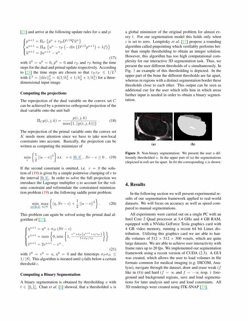
a global minimizer of the original problem for almost ev-ery t. For our segmentation model this holds only whenc is set to zero. Lempitsky et al. [17] propose a roundingalgorithm called pinpointing which verifiably performs bet-ter than simple thresholding to obtain an integer solution.However, this algorithm has too high computational com-plexity for our interactive 3D segmentation task. Thus, wepresent the user different thresholds of u simultaneously. InFig. 3 an example of this thresholding is depicted. In theupper part of the bone the different thresholds are far apart,whereas in regions with a distinct segmentation border thesethresholds close to each other. This output can be seen asadditional cue for the user which tells him in which areasfurther input is needed in order to obtain a binary segmen-tation.

(a) (b)

Figure 3: Non-binary segmentation: We present the user a dif-ferently thresholded u. In the upper part of (a) the segmentations(depicted in red) are far apart. In (b) the corresponding u is shown.

4. Results

In the following section we will present experimental re-sults of our segmentation framework applied to real-worlddatasets. We will focus on accuracy as well as speed com-pared to manual segmentations.

All experiments were carried out on a single PC with anIntel Core 2 Quad processor at 3,4 GHz and 4 GB RAM,equipped with a NVidia GeForce Tesla graphics card with4 GB video memory, running a recent 64 bit Linux dis-tribution. Utilizing this graphics card we are able to han-dle volumes of 512 × 512 × 300 voxels, which are quitelarge datasets. We are able to achieve user interactivity withframe rates up to 20 fps. We implemented our segmentationframework using a recent version of CUDA (2.3). A GUIwas created, which allows the user to load volumes in fileformats common for medical imaging (e.g. DICOM, Ana-lyze), navigate through the dataset, draw and erase weak (flike in (8)) and hard (f = ∞ and f = −∞ resp. ) fore-ground and background regions, save and load segmenta-tions for later analysis and save and load constraints. All3D renderings were created using ITK-SNAP [23].

(a) Original Image (b) Image withadded GaussianNoise

(c) Segmentationusing IsotropicModel

(d) Segmentationusing AnisotropicModel

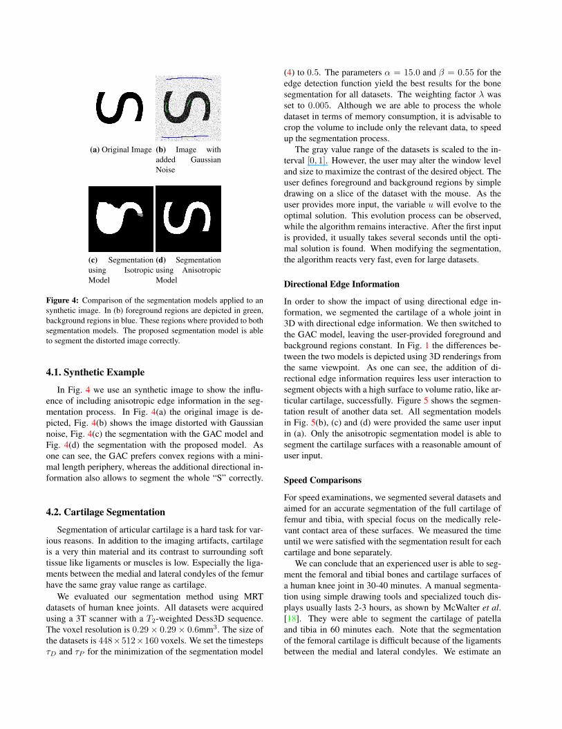
Figure 4: Comparison of the segmentation models applied to ansynthetic image. In (b) foreground regions are depicted in green,background regions in blue. These regions where provided to bothsegmentation models. The proposed segmentation model is ableto segment the distorted image correctly.

4.1. Synthetic Example

In Fig. 4 we use an synthetic image to show the influ-ence of including anisotropic edge information in the seg-mentation process. In Fig. 4(a) the original image is de-picted, Fig. 4(b) shows the image distorted with Gaussiannoise, Fig. 4(c) the segmentation with the GAC model andFig. 4(d) the segmentation with the proposed model. Asone can see, the GAC prefers convex regions with a mini-mal length periphery, whereas the additional directional in-formation also allows to segment the whole “S” correctly.

4.2. Cartilage Segmentation

Segmentation of articular cartilage is a hard task for var-ious reasons. In addition to the imaging artifacts, cartilageis a very thin material and its contrast to surrounding softtissue like ligaments or muscles is low. Especially the liga-ments between the medial and lateral condyles of the femurhave the same gray value range as cartilage.

We evaluated our segmentation method using MRTdatasets of human knee joints. All datasets were acquiredusing a 3T scanner with a T2-weighted Dess3D sequence.The voxel resolution is 0.29× 0.29× 0.6mm3. The size ofthe datasets is 448×512×160 voxels. We set the timestepsτD and τP for the minimization of the segmentation model

(4) to 0.5. The parameters α = 15.0 and β = 0.55 for theedge detection function yield the best results for the bonesegmentation for all datasets. The weighting factor λ wasset to 0.005. Although we are able to process the wholedataset in terms of memory consumption, it is advisable tocrop the volume to include only the relevant data, to speedup the segmentation process.

The gray value range of the datasets is scaled to the in-terval [0, 1]. However, the user may alter the window leveland size to maximize the contrast of the desired object. Theuser defines foreground and background regions by simpledrawing on a slice of the dataset with the mouse. As theuser provides more input, the variable u will evolve to theoptimal solution. This evolution process can be observed,while the algorithm remains interactive. After the first inputis provided, it usually takes several seconds until the opti-mal solution is found. When modifying the segmentation,the algorithm reacts very fast, even for large datasets.

Directional Edge Information

In order to show the impact of using directional edge in-formation, we segmented the cartilage of a whole joint in3D with directional edge information. We then switched tothe GAC model, leaving the user-provided foreground andbackground regions constant. In Fig. 1 the differences be-tween the two models is depicted using 3D renderings fromthe same viewpoint. As one can see, the addition of di-rectional edge information requires less user interaction tosegment objects with a high surface to volume ratio, like ar-ticular cartilage, successfully. Figure 5 shows the segmen-tation result of another data set. All segmentation modelsin Fig. 5(b), (c) and (d) were provided the same user inputin (a). Only the anisotropic segmentation model is able tosegment the cartilage surfaces with a reasonable amount ofuser input.

Speed Comparisons

For speed examinations, we segmented several datasets andaimed for an accurate segmentation of the full cartilage offemur and tibia, with special focus on the medically rele-vant contact area of these surfaces. We measured the timeuntil we were satisfied with the segmentation result for eachcartilage and bone separately.

We can conclude that an experienced user is able to seg-ment the femoral and tibial bones and cartilage surfaces ofa human knee joint in 30-40 minutes. A manual segmenta-tion using simple drawing tools and specialized touch dis-plays usually lasts 2-3 hours, as shown by McWalter et al.[18]. They were able to segment the cartilage of patellaand tibia in 60 minutes each. Note that the segmentationof the femoral cartilage is difficult because of the ligamentsbetween the medial and lateral condyles. We estimate an

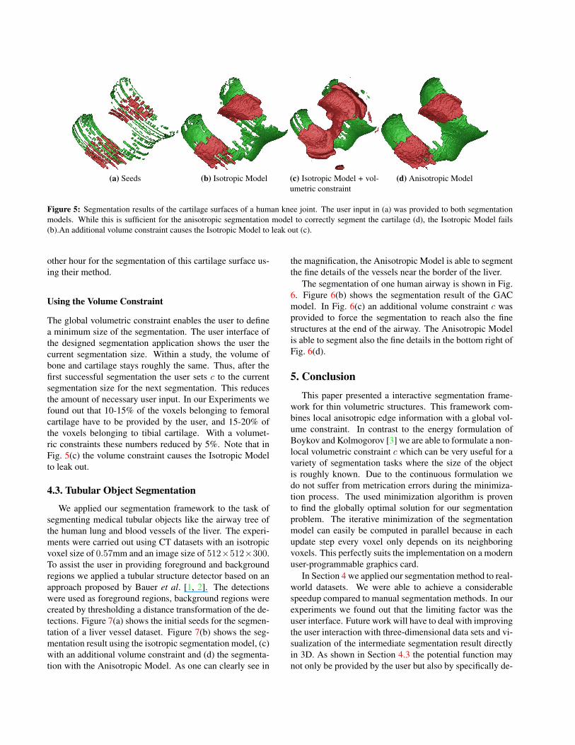
(a) Seeds (b) Isotropic Model (c) Isotropic Model + vol-umetric constraint

(d) Anisotropic Model

Figure 5: Segmentation results of the cartilage surfaces of a human knee joint. The user input in (a) was provided to both segmentationmodels. While this is sufficient for the anisotropic segmentation model to correctly segment the cartilage (d), the Isotropic Model fails(b).An additional volume constraint causes the Isotropic Model to leak out (c).

other hour for the segmentation of this cartilage surface us-ing their method.

Using the Volume Constraint

The global volumetric constraint enables the user to definea minimum size of the segmentation. The user interface ofthe designed segmentation application shows the user thecurrent segmentation size. Within a study, the volume ofbone and cartilage stays roughly the same. Thus, after thefirst successful segmentation the user sets c to the currentsegmentation size for the next segmentation. This reducesthe amount of necessary user input. In our Experiments wefound out that 10-15% of the voxels belonging to femoralcartilage have to be provided by the user, and 15-20% ofthe voxels belonging to tibial cartilage. With a volumet-ric constraints these numbers reduced by 5%. Note that inFig. 5(c) the volume constraint causes the Isotropic Modelto leak out.

4.3. Tubular Object Segmentation

We applied our segmentation framework to the task ofsegmenting medical tubular objects like the airway tree ofthe human lung and blood vessels of the liver. The experi-ments were carried out using CT datasets with an isotropicvoxel size of 0.57mm and an image size of 512×512×300.To assist the user in providing foreground and backgroundregions we applied a tubular structure detector based on anapproach proposed by Bauer et al. [1, 2]. The detectionswere used as foreground regions, background regions werecreated by thresholding a distance transformation of the de-tections. Figure 7(a) shows the initial seeds for the segmen-tation of a liver vessel dataset. Figure 7(b) shows the seg-mentation result using the isotropic segmentation model, (c)with an additional volume constraint and (d) the segmenta-tion with the Anisotropic Model. As one can clearly see in

the magnification, the Anisotropic Model is able to segmentthe fine details of the vessels near the border of the liver.

The segmentation of one human airway is shown in Fig.6. Figure 6(b) shows the segmentation result of the GACmodel. In Fig. 6(c) an additional volume constraint c wasprovided to force the segmentation to reach also the finestructures at the end of the airway. The Anisotropic Modelis able to segment also the fine details in the bottom right ofFig. 6(d).

5. ConclusionThis paper presented a interactive segmentation frame-

work for thin volumetric structures. This framework com-bines local anisotropic edge information with a global vol-ume constraint. In contrast to the energy formulation ofBoykov and Kolmogorov [3] we are able to formulate a non-local volumetric constraint c which can be very useful for avariety of segmentation tasks where the size of the objectis roughly known. Due to the continuous formulation wedo not suffer from metrication errors during the minimiza-tion process. The used minimization algorithm is provento find the globally optimal solution for our segmentationproblem. The iterative minimization of the segmentationmodel can easily be computed in parallel because in eachupdate step every voxel only depends on its neighboringvoxels. This perfectly suits the implementation on a modernuser-programmable graphics card.

In Section 4 we applied our segmentation method to real-world datasets. We were able to achieve a considerablespeedup compared to manual segmentation methods. In ourexperiments we found out that the limiting factor was theuser interface. Future work will have to deal with improvingthe user interaction with three-dimensional data sets and vi-sualization of the intermediate segmentation result directlyin 3D. As shown in Section 4.3 the potential function maynot only be provided by the user but also by specifically de-

(a) Seeds (b) Segmentation usingIsotropic Model

(c) Segmentation us-ing Isotropic Model +volumetric constraint

(d) Segmentation usingAnisotropic Model + vol-umetric constraint

Figure 6: Segmentation of an airway tree: Comparison of different segmentation models. Note the fine details which can only be segmentedusing directional edge information in the segmentation model.

signed detection algorithms. A statistical model based onprevious segmentations which improves with every newlysegmented object would also help to minimize user interac-tion and will be part of our future research.

References[1] C. Bauer, H. Bischof, and R. Beichel. Segmentation of air-

ways based on gradient vector flow. In International Work-shop on Pulmonary Image Analysis, Medical Image Com-puting and Computer Assisted Intervention, pages 191–201,sep 2009. 6

[2] C. Bauer, T. Pock, E. Sorantin, H. Bischof, and R. Beichel.Segmentation of interwoven 3d tubular tree structures utiliz-ing shape priors and graph cuts. Medical Image Analysis,14:174–184, 2010. 6

[3] Y. Boykov and V. Kolmogorov. Computing geodesics andminimal surfaces via graph cuts. In Computer Vision, 2003.Proceedings. Ninth IEEE International Conference on, vol-ume 1, pages 26–33, 2003. 2, 6

[4] X. Bresson. Image segmentation with variational active con-tours. PhD thesis, EPFL, Lausanne, 2005. 2

[5] J. Carter. Dual Methods for Total Variation-based ImageRestauration. PhD thesis, UCLA, Los Angeles, 2001. 3

[6] V. Caselles, R. Kimmel, and G. Sapiro. Geodesic active con-tours. International Journal for Computer Vision, 77:423–451, 1997. 2

[7] A. Chambolle. An algorithm for total variation minimiza-tions and applications. Journal of Mathematical Imaging andVision, 10(1-2):89–97, 2004. 3

[8] S. Chan, T. F.and Esedoglu and M. Nikolova. Algorithmsfor finding global minimizers of image segmentation anddenoising models. SIAM Journal on Applied Mathematics,66:1632–1648, 2006. 4

[9] T. Chan, G. Golub, and P. Mulet. A nonlinear primal-dualmethod for total variation-based image restauration. SIAMJournal of Applied Mathematics, 20(6):1964–1977, 1999. 3

[10] T. Chan and L. Vese. Active contours without edges. ImageProcessing, IEEE Transactions on, 10:266–277, 2001. 3

[11] D. Cremers, M. Rousson, and R. Deriche. A review of statis-tical approaches to level set segmentation: integrating color,texture, motion and shape. International Journal of Com-puter Vision, 72:195–215, 2007. 3

[12] E. Dam, J. Folkesson, M. Loog, P. Pettersen, and C. Chris-tiansen. Efficient automatic cartilage segmentation. In JointDisease Workshop. ITU, 2006. 1

[13] J. Folkesson, E. B. Dam, O. F. Olsen, P. C. Pettersen, andC. Christiansen. Segmenting articular cartilage automati-cally using a voxel classification approach. IEEE Transac-tions on Medical Imaging, 26(1):106–115, Jan. 2007. 1

[14] J. Fripp, S. Crozier, S. Warfield, and S. Ourselin. Automaticsegmentation of articular cartilage in magnetic resonance im-ages of the knee. In 10th International Conference on Med-ical Image Computing and Computer Assisted Intervention,pages 186–194, Brisbane, Australia, 2007. 1

[15] J. Kaftan, H. Tek, and T. Aach. A two-stage approach forfully automatic segmentation of venous vascular structures inliver ct images. In J. P. W. Pluim and B. M. Dawant, editors,Medical Imaging 2009: Image Processing, page 725911,2009. 1

[16] M. Kass, A. Witkins, and D. Terzopolous. Snakes: Activecontour models. International Journal for Computer Vision,1(4):321–331, January 1987. 2

[17] V. Lempitsky, P. Kohli, C. Rother, and T. Sharp. Image seg-mentation with a bounding box prior. In IEEE InternationalConference on Computer Vision, 2009. 4

[18] E. McWalter, W. Wirth, S. M., R. von Eisenhart-Rothe,M. Hudelmaier, D. Wilson, and F. Eckstein. Use of novelinteractive input devices for segmentation of articular carti-

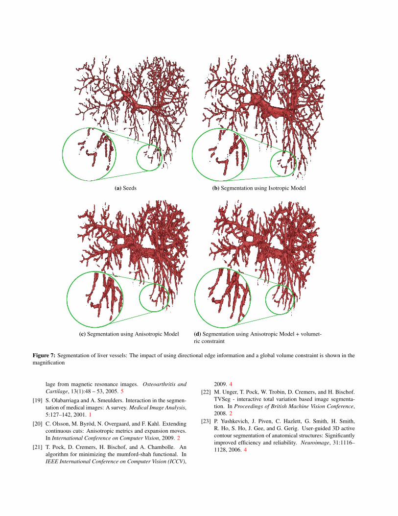
(a) Seeds (b) Segmentation using Isotropic Model

(c) Segmentation using Anisotropic Model (d) Segmentation using Anisotropic Model + volumet-ric constraint

Figure 7: Segmentation of liver vessels: The impact of using directional edge information and a global volume constraint is shown in themagnification

lage from magnetic resonance images. Osteoarthritis andCartilage, 13(1):48 – 53, 2005. 5

[19] S. Olabarriaga and A. Smeulders. Interaction in the segmen-tation of medical images: A survey. Medical Image Analysis,5:127–142, 2001. 1

[20] C. Olsson, M. Byrod, N. Overgaard, and F. Kahl. Extendingcontinuous cuts: Anisotropic metrics and expansion moves.In International Conference on Computer Vision, 2009. 2

[21] T. Pock, D. Cremers, H. Bischof, and A. Chambolle. Analgorithm for minimizing the mumford-shah functional. InIEEE International Conference on Computer Vision (ICCV),

2009. 4[22] M. Unger, T. Pock, W. Trobin, D. Cremers, and H. Bischof.

TVSeg - interactive total variation based image segmenta-tion. In Proceedings of British Machine Vision Conference,2008. 2

[23] P. Yushkevich, J. Piven, C. Hazlett, G. Smith, H. Smith,R. Ho, S. Ho, J. Gee, and G. Gerig. User-guided 3D activecontour segmentation of anatomical structures: Significantlyimproved efficiency and reliability. Neuroimage, 31:1116–1128, 2006. 4