A Three-Dimensional Variational (3DVAR) Data Assimilation

System For Use With MM5

Dale Barker, Wei Huang, Yong-Run Guo, and Al Bourgeois

MMM Division, NCAR, P.O. Box 3000, Boulder, CO, 80307-3000, USA.

Table Of Contents

T able O f C ontents.............................................................................................................P reface ........................................................................................................................... iii

A cknow ledgem ents ................................................................................. iv

1. Introduction ..................................................... 1............

a) The Data Assimilation Problem ............................................... 2

b) Variational Data Assimilation ............................................................................... 2

c) Motivation for developing a 3DVAR system for use with MM5...........................5

2. Overview Of 3DVAR In The MM5 Modeling System ............................................... 7

a) Background Preprocessing ................................................................................ 8

b) The Observation Preprocessor (3DVAR_OBSPROC) ........................................... 8

c) Background Error Calculation............................................................................ 9

e) Update Boundary Conditions .................................................... 12

3. The Observation Preprocessor (3DVAR_OBSPROC) ........................................ 13

a) Observation Preprocessor Tasks.................................................... 13

b) Quality Control Flags used in 3DVAR_OBSPROC and 3DVAR ........................ 15

4. The 3D V A R System .................................................................................................. 17

a) O verview ............................................................................................................... 17

b) 3DVAR Preconditioning Method.......................................................................... 19

c) 3DVAR Source Code Organization ...................................................................... 22

5. Horizontal Background Error Covariances Via Recursive Filters: Uh ...................... 26

a) The Recursive Filter Algorithm.............................................................................26

b) The Use Of Recursive Filters in 3DVAR..............................................................30

6. Vertical Background Error Covariances Via EOF projection: Uv............................. 33

7. Physical Transform Via Change Of Variable: Up........................................35

8. Climatological Background Errors Via The "NMC-Method" .................................. 37

a) Calculation of eigenvectors/values of vertical background errors: ....................... 37

b) Calculation of balance regression statistics...........................................................38

i

c) Calculation Of Recursive Filter Characteristic Lengthscales ................................ 39

9. Updating MM5 Lateral Boundary Conditions .......................................................... 41

10. Parallelization ................................................ 42

a) Setup D ata Structures ............................................................................................ 42

b) Minimization Of The Cost Function ................................................ 44

c) Computation And Output Of Analysis And Diagnostics ...................................... 46

d) Fortran90 Performance Issues ................................................ 47

11. R eferences ............................................................................................................... 48

Appendix A - The Governing Equations ................................................. 51

Appendix B - Example Application: The Introduction Of A New Observation Type .60

A ppendix C - U ser G uide ............................................................................................. 63

Appendix D - 3DVAR Namelist Parameters ................................................... .. 65

Appendix E - Example 3DVAR Output Files .............................................................. 67

Appendix F - Acronyms Used ...................................................................................... 68

ii

Preface

This document describes the three-dimensional variational (3DVAR) data assimilation

system designed and built in the MMM Division of NCAR for use with the MM5

modeling system. This, and additional, documentation can be found online at the MM5

3DVAR web-site:

http://www.mmm.ucar.edu/3dvar

The 3DVAR system described here was also adopted in June 2001 as the starting point

for 3DVAR development for the Weather Research Forecast (WRF) model. This version

of the technical documentation focuses on the use of 3DVAR within the MM5 modeling

environment.

iii

Acknowledgements

Many people, too numerous to mention, have contributed to the development of a

3DVAR system for MM5. Their input has greatly increased the accuracy, efficiency,

robustness and clarity of the code. We are very appreciative of their efforts. We look

forward to continued feedback in future to allow us to improve the system still further.

We would also like to thank the reviewers of this technical note (Wei Wang, Riffat Rizvi,

and Carey Kerschner) for their comments and edits which helped to clarify the document.

We acknowledge the Taiwanese Civil Aeronautics Administration (CAA), the United

States Air Force Weather Agency (AFWA) and the United States Weather Research

Program (USWRP) for their support of this effort.

iv

1. Introduction

This document provides a reference for technical details of the 3DVAR system for MM5.

The code has been designed to be a community data assimilation system flexible enough

to allow a variety of research studies to be performed (e.g. impact of new observation

types, globally relocatable etc). In addition, the code has from the start of the project been

geared towards operational implementation. Thus, the issues of computational efficiency

and robustness have also been major design features. Results from initial operational

applications of the 3DVAR system with MM5 can be found in Barker et al. (2003).

In the remainder of this introductory section, a brief discussion of the general data

assimilation problem is given followed by a short introduction to variational data

assimilation. Finally, motivations for developing the 3DVAR system for MM5 are

outlined. Section 2 provides an overview of the 3DVAR system in MM5 applications

including a description of the various components specially written for use with 3DVAR.

Section 3 describes one of these components - the observation preprocessor used to

quality control and format observations ready for input into 3DVAR. The 3DVAR code

itself is reviewed in section 4. Sections 5 to 7 describe in turn the three components of the

3DVAR control variable transform used to allow practical minimization of the 3DVAR

cost-function. The complexity and sensitivity of components of a variational data

assimilation system requires constant checks on the code and input data. In addition to

the two primary sources of input data (observations and a previous background forecast),

estimates of observation and background error are required to compute the analysis. In

the current system, the background error covariance matrix is approximated via the

"NMC-method" of averaging forecast differences. The code developed for this purpose is

described in section 8. In order to run a bounded forecast model from the analysis, lateral

boundary conditions must be modified to take account of the differences between

background and analysis fields. The "update_bc" code performs this task and is described

in section 9. In section 10 a description is given of the methods used to permit 3DVAR to

be run on multiple processor platforms. The appendices contain background and technical

information on various aspects of the 3DVAR system.

1

a) The Data Assimilation Problem

A data assimilation system combines all available information on the atmospheric state in

a given time-window to produce an estimate of atmospheric conditions valid at a

prescribed analysis time. Sources of information used to produce the analysis include

observations, previous forecasts (the background or first-guess state), their respective

errors and the laws of physics. The analysis can be used in a number of ways, including:

* Providing initial conditions for a numerical weather forecast (initialization).

* Studying climate through the merging of observations and numerical models

(reanalysis).

* Assessing the impact of individual components of the existing observation

network via Observation System Experiments (OSEs).

* Predicting the potential impact of proposed new components of a future

observation network via Observation System Simulation Experiments (OSSEs).

The importance of accurate initial conditions to the success of an assimilation/forecast

numerical weather prediction (NWP) system is well known. The relative importance of

forecast errors due to errors in initial conditions compared to other sources of error such

as physical parameterizations, boundary conditions and forecast dynamics depends on a

number of factors e.g. resolution, domain, data density, orography as well as the forecast

product of interest. However, judging from the current/future-planned resources

(computational and human) of both operational and research communities being devoted

to data assimilation, better initial conditions are increasingly considered vital for a whole

range of NWP applications. Initial applications of the MM5 3DVAR system have

focused on providing initial conditions from which to integrate MM5 forecasts. Future

use of the system for regional climate modeling, OSEs and OSSEs is an exciting

possibility.

b) Variational Data Assimilation

2

In recent years, much effort has been spent in the development of variational data

assimilation systems to replace previously used schemes e.g. the Cressman (MM5),

Newtonian nudging (FDDA -MM5), optimum interpolation (01 - NCEP, ECMWF,

HIRLAM, NRL, etc) and analysis correction (UKMO) algorithms. Practical

considerations have led to a variety of alternative implementations of VAR systems.

The basic goal of the MM5 3DVAR system is to produce an "optimal" estimate of the

true atmospheric state at analysis time through iterative solution of a prescribed cost-

function (Ide et al. 1997)

l0b1 -b 1J(x)=Jb +J =(x-x) T B- (x-xb)+ (yyo)T (E+F)-(y-yo). (1)2 2

The VAR problem can be summarized as the iterative solution of Eq. (1) to find the

analysis state x that minimizes J(x). This solution represents the a posteriori maximum

likelihood (minimum variance) estimate of the true state of the atmosphere given the two

sources of a priori data: the background (previous forecast) xb and observations y°

(Lorenc 1986). The fit to individual data points is weighted by estimates of their errors:

B, E and F are the background, observation (instrumental) and representivity error

covariance matrices respectively. Representivity error is an estimate of inaccuracies

introduced in the observation operator H used to transform the gridded analysis x to

observation space y=Hx for comparison against observations. This error will be

resolution dependent and may also include a contribution from approximations (e.g.

linearizations) in H.

The quadratic cost function given by Eq. (1) assumes that observation and background

error covariances statistically are described using Gaussian probability density functions

with zero mean error. Alternative cost functions maybe used which relax these

assumptions (e.g. Dharssi et al. 1992). Eq. (1) addition eally neglects correlations between

observation and background errors.

3

The use of adjoint operations, which can be viewed as a multidimensional application of

the chain-rule for partial differentiation, permits efficient calculation of the gradient of

the cost-function. Modern minimization techniques (e.g. Quasi-Newton, preconditioned

conjugate gradient) are used to efficiently combine cost function, gradient and the

analysis information to produce the "optimal" analysis.

The theoretical problem of minimizing the cost function J(x) is equivalent to the

previous-generation 01 technique in the linear case. Despite this equivalence, previously

developed operational 3/4DVAR systems e.g. NCEP (1992), ECMWF (1996/8), Meteo-

France (1998/2000), UKMO (1999) have led to improved forecast scores relatively

quickly after implementation through their more flexible design. Below are listed

practical advantages of VAR systems over their predecessors.

* Observations can easily be assimilated directly without the need for prior

retrieval. This results in a consistent treatment of all observations and, as the

observation errors are less correlated (with each other and the background errors),

practical simplifications to the analysis algorithm.

* The VAR solution is found using all observations simultaneously, unlike the 01

technique for which a data selection into artificial sub-domains is required.

* Asynoptic data can be assimilated near its validity time. This is implicit to

4DVAR but can also be achieved using a "rapidly-updating" 3DVAR technique.

* Balance (e.g. weak geostrophy, hydrostatic) constraints can be built into the

preconditioning of the cost-function minimization. In 4DVAR, use is also made

of the implicit balance of the forecast model.

Having expounded the advantages of variational data assimilation it is wise to also

recognize its weaknesses. Although the variational analysis is frequently described as

"optimal", this label is subject to a number of assumptions. Firstly, given both imperfect

4

observations and prior (e.g. background) information as inputs to the assimilation system,

the quality of the output analysis depends crucially on the accuracy of prescribed errors.

Secondly, although the variational method allows for the inclusion of linearized

dynamical/physical processes, in reality real errors in the NWP system may be highly

nonlinear. This limits the usefulness of variational data assimilation in highly nonlinear

regimes e.g. the convective scale or in the tropics. It is hoped that the 3DVAR system

will be used in future studies to investigate these research topics.

In the development of variational data assimilation systems at the operational centers,

3DVAR has been seen as a necessary prerequisite to the ultimate goal of four-

dimensional (e.g. 4DVAR/Kalman-filter-type) assimilation algorithms. Their initial

concentration on 3DVAR has been partly motivated by a lack of computing resources

(with the current exceptions of ECMWF and Meteo-France which now run 4DVAR

operationally). Without the cut-off time restrictions of the weather centers, the research

community has tended to bypass 3DVAR to concentrate on applications of 4DVAR to

new/asynoptic data types e.g. Doppler radar.

c) Motivation for developing a 3DVAR system for use with MM5.

Given the pre-existence of an MM5 4DVAR capability (Zou et al. 1997), it is perhaps

necessary to discuss the reasons for developing a new 3DVAR system for use with the

MM5. The major goal for the project has been to design a single VAR system suitable for

operational implementation at the Taiwanese Civil Aviation Authority (CAA) and the

U.S. Air Force Weather Agency (AFWA) in Omaha, Nebraska. An additional goal has

been to release the 3DVAR code to the data assimilation research community and

provide support to users. Given a period of 2 1/2 years to achieve these goals, the strategy

has been to concentrate limited resources into producing a research quality 3DVAR data

assimilation system that is also computationally efficient and robust. This choice was

made for the following reasons:

5

* 3DVAR is computationally much cheaper than 4DVAR - in real-time

applications 4DVAR may not produce analyses in time for dissemination to

forecasters.

* A well-designed 3DVAR system provides a sound base from which to potentially

upgrade to a 4DVAR capability. Many of the algorithms required by 4DVAR

(observation operators, minimization packages, preconditioning methods, balance

constraints, background error covariances, data assimilation diagnostics, etc) are

contained within 3DVAR, which therefore provides an environment for

researchers to investigate these crucial aspects of the data assimilation system.

The only significant omission required for 4DVAR is a forecast adjoint model

and, in the case of incremental 4DVAR, the corresponding linear model used to

describe the evolution of finite perturbations. Given these additional components,

extension to a 4DVAR capability is relatively straightforward.

Even with the continual increase in computing power, it is far from obvious if the

additional available CPU should be used to implement more expensive data assimilation

algorithms (e.g. 4DVAR, Kalman Filters). Greater benefit may be seen using the extra

computing power to permit inclusion of additional high-density (underused and

expensive) observations in the cheaper 3DVAR algorithm. The answer will be

application-dependent, but it is highly probable that 3DVAR will continue to be a

valuable data assimilation tool for the foreseeable future.

6

2. Overview Of 3DVAR In The MM5 Modeling System

This section provides an overview of the 3DVAR system as used in the MM5 modeling

environment. The basic layout is illustrated in Fig. (1) for both cold-starting mode, where

the background forecast originates from another model and/or grid, and cycling mode

where the background forecast is a short-range MM5 forecast from a previous 3DVAR

analysis. The three input (first guess, observation and background error) and output

(analysis) files are shown as circles. Highlighted rectangles indicate code especially

written for use with 3DVAR and MM5. Clear rectangles represent preexisting code.

I

FIG. 1. The various components of the 3DVAR system (highlighted) and their interaction with pre-

existing components of the MM5 modeling system. Note the background preprocessing is only

required if 3DVAR is being run in "cold-starting" mode.

7

i

The following is a summary of the various components of the system. Further details on

individual algorithms can be found in subsequent sections.

a) Background Preprocessing

In cold-starting mode, standard MM5 preprocessing programs may be used to reformat

and interpolate forecast fields from a variety of sources to the target MM5 domain. These

packages are:

* TERRAIN - defines domain, orography, land use etc.

* PREGRID - reads background forecast in native format e.g. RUC, ETA, AVN,

ECMWF etc.

* REGRIDDER - horizontally interpolates background to MM5 domain.

* INTERPF - vertically interpolates background field to MM5 sigma-height levels.

For further details on any of the above MM5 preprocessing packages, refer to the

documentation on the MM5 web-page: http://www.mmm.ucar.edu/mm5. In cycling

mode, background processing is not required as the background field x input to 3DVAR

is already on the MM5 grid.

b) The Observation Preprocessor (3DVAR_OBSPROC)

The observation preprocessor provides the observations y° for ingest into 3DVAR. The

program 3DVAR_OBSPROC has been specially written for use with the MM5 3DVAR

system. It performs the following functions:

* Reads in observation file in decoder (MM5 LITTLE_R format).

* Reads in run-time parameters from a namelist file.

* Performs spatial and temporal checks to select only observations located within

the target domain and within a specified time-window.

* Calculates heights for observations whose vertical coordinate is pressure.

8

* Merges duplicate observations (same location, place, type) and chooses

observation nearest analysis time for stations with observations at several times.

* Estimates the error for each observation.

* Outputs observation file in ASCII 3DVAR format.

Further details may be found in Section 3.

c) Background Error Calculation

Background error covariance statistics are used in the 3DVAR cost-function to weight

errors in features of the background field. The assimilation system will filter those

background structures that have high error relative to more accurately known background

features and observations. In reality, errors in the background field will be synoptically-

dependent i.e. vary from day to day depending on the current weather situation. Current

implementations of 3DVAR however, tend to use climatological background errors

although research is ongoing into the specification and use of background "errors of the

day".

The NMC-method (Parrish and Derber 1992) is a popular method for estimating

climatological background error covariances. In this process, background errors are

assumed to be well approximated by averaged forecast difference (e.g. month-long series

of 24hr - 12hr forecasts valid at the same time) statistics:

B=(xb xt xb xt)T = (xT+24 T+12 X T +24 T+12)T (2)

where x is the true atmospheric state and e b is the background error. The overbar

denotes an average over time and/or space. Technical details of the NMC-method code

developed in NCAR/MMM may be found in section 8. In the current MM5 3DVAR, the

background errors are computed for a variety of resolutions and a seasonal dependence is

9

introduced simply by using forecast difference statistics valid at different times of the

year (e.g. winter, summer).

It is clear that the background errors should estimate errors in the analysis/forecast used

as starting point for the 3DVAR minimization. In cold-starting mode, the background

field originates from a different model (e.g. AVN, CWBGM). In contrast, a cycling

application requires errors representative of a short-range forecast run from a previous

3DVAR analysis. Background errors will vary between each application and should

ideally be tuned for each domain. This is time-consuming, but important, work. A

recalculation of background error should be considered whenever the background field

changes. Scenarios where this might occur include:

* Using an alternative source for the background field in cold-starting mode.

* The cold-starting background has been upgraded (e.g. change of resolution,

additional observations used in a global analysis background).

* Change to MM5 configuration in a cycling run.

The initial period of a new cycling application must initially use background errors

interpolated from another source of similar resolution/location. Once the new domain has

been running for a period (e.g. 1 month) a better estimate of background error may be

obtained. This is an iterative process - changing the background error used in 3DVAR

will again modify background errors of the resulting short-range forecast used as

background.

The calculation of background error covariances requires significant resources that are

not always available. Given this limitation, and the fact that the background errors

derived by the "NMC-method" are climatological estimates, approximations are

inevitable. 3DVAR includes a number of namelist variables that allow some tuning of the

background error files at run-time. These, and other namelist options are described in the

next section.

10

d) 3DVAR System Overview

Although the 3DVAR code is completely new, the particular 3DVAR implementation

described below is similar in basic design to that implemented operationally at the UK

Meteorological Office in 1999 (Lorenc et al. 2000). In summary, the main features of the

MM5 3DVAR system include:

* Incremental formulation of the model-space cost function given by Eq. (1).

* Quasi-Newton minimization algorithm (Liu and Nocedal, 1989).

* Analysis increments on unstaggered "Arakawa-A" grid. In the MM5

environment, the input background wind field is interpolated from the Arakawa-B

grid of MM5. On output, the unstaggered analysis wind increments are

interpolated to the MM5 B-grid.

* Analysis performed on the sigma-height levels of MM5.

* Jb preconditioning via a "control variable transform" U defined as B=UUT .

* Preconditioned control variables are chosen as streamfunction, velocity potential,

unbalanced pressure and a choice between specific or relative humidity.

* Linearized mass-wind balance (including both geostrophic and cyclostrophic

terms) used to define a balanced pressure.

* Climatological background error covariances estimated via the NMC-method of

averaged forecast differences. Values are tuned by comparison with estimates

derived from observation minus background differences (innovation vector)

statistics.

* Representation of the horizontal component of background error via isotropic

recursive filters. The vertical component is applied through projection onto

climatologically averaged eigenvectors of vertical error (estimated via the NMC-

method. Horizontal/vertical errors are non-separable (horizontal scales vary with

vertical eigenvector).

Further details can be found in links from the NCAR/MMM 3DVAR web site

(http://www.mmm.ucar.edu/3dvar) including links to results of extended testing as well

11

as the code (Fortran90 transformed to html using software designed in NCAR/MMM).

The code itself contains a significant level of documentation.

e) Update Boundary Conditions

In order to run MM5 (or any other forecast model supported by the 3DVAR system)

using the 3DVAR analysis as initial conditions, the lateral boundary conditions must first

be modified to reflect differences between background forecast and analysis. This process

is described in section 10.

12

3. The Observation Preprocessor (3DVAR_OBSPROC)

The observation preprocessor provides the observations y° for ingest into 3DVAR and

has been specially developed for MM5 applications of 3DVAR. The

3DVAR_OBSPROC program makes use of Fortran90 and requires an F90-friendly

compiler. It has been successfully run on DEC-Alpha, IBM-SP, Fujitsu VPP5000, NEC-

SX5 and PC/Linux machines.

a) Observation Preprocessor Tasks

The observation preprocessor performs the following functions:

1. Reads in observation file in decoder (LITTLER) format.

This format is that output by MM5 decoder routines and previously used in the

preexisting MM5 LITTLE_R analysis package. This format was adopted as input to

3DVAR_OBSPROC in order to allow easy comparison of 3DVAR with LITTLE_R

(which 3DVAR is intended to replace). A description of the LITTLE_R data format can

be found at:

http:llwww.mmm.ucar.edu/mm5/documents/MM5_tut_Web_notes/App_C/little_r.html

2. Reads in run-time parameters from a namelist file. An example is given below:

&recordlobs_gts_filename = '/mmmtmp/bresch/3dv/obs',obs err filename = 'obserr.txt',obs_gpsfilename = 'NOGPS',first_guess_file = '/mmmtmp/bresch/3dv/MMINPUT_DOMAIN2',

/

&record2time earlier = -90,time_analysis = '2001-06-27_12:00:00',timelater = 90,

/

13

&record3maxnumber of obs = 58000,fatalifexceedmax obs = .TRUE.,

/

&record4

qc_test_vert_consistency = .TRUE.,qc_test_convectiveadj = .TRUE.,qc_test above_lid = .TRUE.,removeabovelid = .TRUE.,ThiningSATOB = .FALSE.,ThiningSSMI = .FALSE.,

/

&record5print_gts_read = .TRUE.,print_gpspwread = .TRUE.,printrecoverp = .TRUE.,printduplicateloc = .TRUE.,print_duplicate_time = .TRUE.,print recoverh = .TRUE.,print_qcvert = .TRUE.,printqcconv = .TRUE.,print_qc_lid = .TRUE.,printuncomplete = .TRUE.,user defined area = .FALSE.,

/

&record6x_left = 1.,

x_right = 100.,

y_bottom = 1.,

y_top = 100.,

/

3. Performs spatial and temporal checks to select only observations located within the

target domain and within a specified time-window.

4. Calculates heights for observations whose vertical coordinate is pressure.

5. Merges duplicate observations (same location, place, type) and chooses observation

nearest analysis time for stations with observations at several times.

6. Estimates the error for each observation. Values are input from the "obserr.txt" file

containing observation errors at standard pressure levels for a number of different

observation types. The errors tabulated in file "obserr.txt" originate from NCEP but have

been modified at NCAR after comparisons against O-B data.

14

7. Outputs observation file in ASCII MM5 3DVAR format read for input to 3DVAR. An

example header of the observation file is given below.

TOTAL = 8170, MISS. =-888888.,SYNOP = 1432, METAR = 164, SHIP = 86, TEMP = 180, AMDAR = 0,AIREP = 265, PILOT = 0, SATEM = 0, SATOB = 6043, GPSPW = 0,SSMT1 = 0, SSMT2 = 0, TOVS = 0, OTHER = 0,PHIC = 28.50, XLONC = 116.00, TRUE1 = 10.00, TRUE2 = 45.00,TSO = 275.00, TLP = 50.00, PTOP = 7000., PSO =100000.,IXC = 67, JXC = 81, IPROJ = 1, IDD = 1, MAXNES= 10,NESTIX= 67, 67, 67, 67, 67, 67, 67, 67, 67, 67,NESTJX= 81, 81, 81, 81, 81, 81, 81, 81, 81, 81,NUMC = 1, 1, 1, 1, 1, 1, 1, 1, 1, 1,DIS = 135.00, 0.00, 0.00, 0.00, 0.00, 0.00, 0.00, 0.00, 0.00, 0.00,NESTI = 1, 1, 1, 1, 1, 1, 1, 1, 1, 1,NESTJ = 1, 1, 1, 1, 1, 1, 1, 1, 1, 1,INFO = PLATFORM, DATE, NAME, LEVELS, LATITUDE, LONGITUDE, ELEVATION, ID.SRFC = SLP, PW (DATA,QC,ERROR).EACH = PRES, SPEED, DIR, HEIGHT, TEMP, DEW PT, HUMID (DATA,QC,ERROR)*LEVELS.INFO FMT = (A12,1X,A19,1X,A40,1X,I6,3(F12.3,11X),6X,A5)SRFCFMT = (F12.3,I4,F7.2,F12.3,I4,F7.2)EACH_FMT = (3(F12.3,I4,F7.2),11X,3(F12.3,I4,F7.2),11X,1(F12.3,I4,F7.2)))

....... observations.... .

The header contains information on the number of observations for each type and the grid

that has been used to select observations. The final three lines above define the format

used to store particular observations which follow the header and which are subsequently

read by 3DVAR. The observation preprocessor also has the capability to input

observations in BUFR format. This latter format is not used in MM5 applications.

8. 3DVAR_OBSPROC outputs numerous diagnostics files that detail the quality control

decisions taken and error estimates used.

b) Quality Control Flags used in 3DVAR_OBSPROC and 3DVAR

A variety of quality control checks are performed by the observation preprocessor.

Quality control flags are set for all observations and output ready for input into 3DVAR.

The following flags are currently used:

missing_data = -88, & ! Data is missing with the value of missing_routside of domain = -77, & Data outside horizontal domain

! or time window, data set to missing_rwrong_direction = -15, & ! Wind vector direction <0 or> 360

=> direction set to missing_rnegative_spd = -14, & i Wind vector norm is negative

=> norm set to missing_rzerospd = -13, & ! Wind vector norm is zero

15

wrong_winddata

zerot td

t_fail_supainver

wrong_t_sign

abovemodel lid

farbelow model surface

belowmodel surface

standard_atmosphere

from_background

fails error max

fails_buddy_check

nobuddies

good_quality

convective_adjustment

surfacecorrection

Hydrostatic_recover

ReferenceOBS recover

Othercheck

= -12,

= -11,

= -10,

= - 9,

= - 8,

= - 7,

= - 6,

= - 5,

= - 4,

= - 3,

= - 2,

= - 1,

= 0,

= 1,

2,

= 3,

= 4,

&

&

&

&

&

&

&

&

&

&

&

&

&

&

&

&

&

= 88

! => norm set to missing_r!Spike in wind profile!=>direction and norm set to missing_r! t or td = 0 => t or td, rh and qv! are set to missing_r,!superadiabatic temperature

! Spike in Temperature profile!! height above model lid

=> no action! height far below model surface!=> no action

!height below model surface=> no action

! Missing h, p or t! =>Datum interpolated from standard atm! Missing h, p or t! =>Datum interpolated from model!Datum Fails error max check! => no action

! Datum Fails buddy check! => no actionDatum has no buddies

! => no action! OBS datum has good quality

! convective adjustment check! =>apply correction on t, td, rh and qvSurface datum=> apply correction on datum

! Height from hydrostatic assumption with! the OBS data calibration! Height from reference state with OBS! data calibration! passed other quality check

16

4. The 3DVAR System

As discussed above, the role of the 3DVAR assimilation system is to use the three input

data sources xb, y° and B to produce analysis increments xai to be recombined with the

background xb in order to produce an analysis xa = xb + I x" from which to run MM5.

The operator I represents post-processing of the analysis increments in 3DVAR e.g.

modifications to ensure the humidity analysis is within physical limits.

a) Overview

NamelistFile

I ..... .............. ................... ".......).. l tr T nnn"

I iostic

File

FIG. 2: Illustration of the major steps taken during the 3DVAR analysis precedure.

The top-level structure of 3DVAR is shown in Fig. 2. The 3DVAR runs under the WRF

model framework to permit access to WRF MPP software, required for applications of

17

B--.......m.....-----...............m..m...mm....

I :

........ 1"

3DVAR on multiple processor platforms. In future, this arrangement will also allow easy

access to other parts of the WRF system (e.g. I/O) from 3DVAR (and vice versa). The

3DVAR algorithm is called as a "mediation layer" subroutine from the WRF driver.

The following summarizes the role of each step in the 3DVAR algorithm:

1. Setup MPP: Details of the run configuration are read in from a WRF namelist

file. Tile, memory and domain dimension are calculated and stored.

2. Read [3DVAR] Namelist: 3DVAR run-time options are read in from a namelist

file. These options are described more fully in Appendix D.

3. Setup Background: The background field x b is read in (MM5 format for MM5

applications, WRF format for WRF). Variables required by 3DVAR are stored in

the xb Fortran90 derived data type (e.g. xb % u, xb % v etc). Any additional fields

present in the input file are ignored.

4. Setup Background Errors: Components of the background error (eigenvectors,

eigenvalues, lengthscales and balance regression coefficients) are read in

(currently in MM5 format) and stored in the be derived data type (e.g. be % vl, be

% reg_coeffetc).

5. Setup Observations: Observations y° and metadata (output from the observation

preprocessor) are read (in either MM5 3DVAR ASCII or BUFR format) and

stored in the ob derived data type (e.g. ob % synop % lat, ob % sonde % u, etc).

Basic quality control checks are again applied (e.g. domain checks) and an initial

quality control flag is assigned.

6. Calculate O-B: For valid data, the innovation vector y° - yb is calculated and

stored in the iv derived data type (of similar design to the ob structure but

including additional metadata). The transform yb = H(xb) of the full-resolution

background x b to observation space uses the nonlinear observation operator H.

This transform involves both a change from model to observation variable and

interpolation from grid points to the observation location. A "maximum error

check" is applied to all values within the innovation vector iv which compares the

O-B value against a maximum value defined as a multiple of the observation error

18

for each observation. Various namelist parameters exist to tune QC checks as well

as ones to choose which QC flags to ignore.

7. Minimize Cost Function: The minimization of the 3DVAR cost function

proceeds iteratively as described below. Diagnostic output includes cost function

and gradient norm values for each iteration.

8. Calculate Analysis: Having found the control variables that minimize the cost

function, a final transform of the analysis increments to model (i.e. gridded u, v,

T, p, q) space is performed. The increments are added to the background values to

produce the analysis. Finally, checks are performed to ensure certain variables are

within physically reasonable limits (e.g. relative humidity is greater than zero and

less that 100%). The increments are adjusted if analysis values fall outside this

range.

9. Compute Diagnostics: Assimilation statistics (minimum, maximum, mean and

root mean square) are calculated and output for study e.g. O-B, O-A statistics for

each observation type, A-B (increment) statistics for each model variable. Output

files are described in Appendix E.

10. Output Analysis: Both analysis and analysis increments are output.

11. Tidy Up: Dynamically allocated memory is deallocated and summary run-time

data output.

The "outer loop" seen in Fig. 2 permits the recalculation of the innovation vector using

the analysis as an improved "background". The recalculation of O-B uses the full

nonlinear observation operator H and hence provides a way if introducing nonlinearities

into the analysis procedure. In addition, quality control checks based on maximum O-B

values can be repeated. This equates to a crude "variational quality control" through the

possibility that observation previously rejected due to too large an O-B value may be

accepted in subsequent outer loops if the new O-B drops below the specified maximum

value.

b) 3DVAR Preconditioning Method

19

This subsection contains some of the mathematics behind the solution method chosen for

the 3DVAR system. As stated above, the basic problem is to find the analysis state xa that

minimizes a chosen cost function, here given by Eq. (1). For a model state x with n

degrees of freedom, calculation of the background term Jb of the cost function requires

-0O(n 2) calculations. For a typical NWP model with n - 106 - 107 (number of grid-points

times number of independent variables) direct solution is prohibitively expensive.

One practical solution to this problem is to perform a preconditioning via a control

variable v transform defined by x' = Uv, where x' = x - xb. The transform U is chosen to

approximately satisfy the relationship B=UUT. Using the incremental formulation

(Courtier et al. 1994) and the control variable transform, eq. (1) may be rewritten

J(v) = Jb + J = T-vT +-(y o -HUv (E +F) l(yO -HUv). (3)2 2

where y° = y° - H(xb) is the innovation vector and H is the linearization of the potentially

nonlinear observation operator H used in the calculation of yO'. In this form, the

background term is essentially diagonalized, reducing the number of calculations

required from O(n2) to O(n). In addition, the background error covariance matrix equals

the identity matrix I in control variable space, hence preconditioning the minimization

procedure.

The use of the incremental method has a number of advantages. Firstly, use of linear

control variable transforms allows the straightforward use of adjoints in the calculation of

the gradient of the cost function. Secondly, any imbalance introduced through the

analysis procedure is limited to the (small) increments that are added to the balanced first

guess. This generally leads to a more balanced analysis than that obtained using a

technique in which the full-field analysis is constructed.

The transformation x' = Uv must be designed to ensure the validity of the B=UUT

relationship. One goal is to transform to variables whose errors are largely uncorrelated

20

with each other thus reducing B to block-diagonal form. In addition, each component of v

is essentially scaled by the appropriate background error variance to allow an accurate

penalization in the transformed b cost function.

Another goal of the control variable transform is to represent spatial correlations in an

accurate and simple form. Examples of spatial transforms typically employed include

Fourier transforms, empirical orthogonal functions (principal component analysis) and

Chebyshev polynomials. These methods permit a projection of background errors onto

orthogonal directions whose cross-correlations are, by definition, zero. This error

compression greatly reduces the cost of calculating b but is sometimes accompanied by

approximations which may not be realistic. For example, in the case of spectral

transforms, the errors are assumed to be homogeneous and isotropic. Despite this

restriction, the spectral technique is used in many implementations of 3/4DVAR to

represent horizontal error correlations (e.g. ECMWF, NCEP, UKMO, Meteo-France,

HIRLAM and CMC). An alternative spatial transform is the recursive filter as used in the

MM5 and ETA 3DVAR systems which in principle allows the specification of

anisotropic and inhomogeneous error correlations.

Grid deformation techniques may be included in the "control variable" transform to

introduce anisotropic and imhomogeneous error correlations. One such method is the

semi-geostrophic horizontal transform of Desroiziers (1997). This method essentially

provides higher resolution and anisotropic error correlations in frontal regimes but has

limited applicability in regimes in which the semi-geostrophic approximations are invalid

e.g. in the tropics. Transformation of the vertical coordinate of the analysis may also be

used, e.g. the isentropic vertical co-ordinate of Benjamin (1989). As well as providing

higher horizontal and vertical resolution in baroclinic zones and hence anisotropic

correlations, the isentropic coordinate may potentially lead to an improve analysis given

the isentropes are material surfaces in adiabatic conditions. Unlike the semi-geostrophic

transform, analysis on isentropic surfaces is applicable to the tropics and also provides a

framework for the use of the Ertel potential vorticity

21

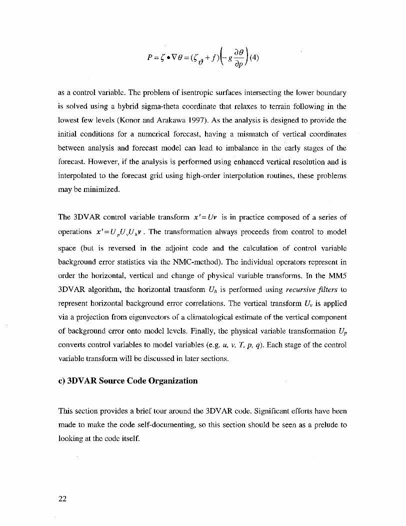
P=-.VO=(f +of)( -a (4)

as a control variable. The problem of isentropic surfaces intersecting the lower boundary

is solved using a hybrid sigma-theta coordinate that relaxes to terrain following in the

lowest few levels (Konor and Arakawa 1997). As the analysis is designed to provide the

initial conditions for a numerical forecast, having a mismatch of vertical coordinates

between analysis and forecast model can lead to imbalance in the early stages of the

forecast. However, if the analysis is performed using enanced vertical resolution and is

interpolated to the forecast grid using high-order interpolation routines, these problems

may be minimized.

The 3DVAR control variable transform x'=Uv is in practice composed of a series of

operations x'= UpUVUhV. The transformation always proceeds from control to model

space (but is reversed in the adjoint code and the calculation of control variable

background error statistics via the NMC-method). The individual operators represent in

order the horizontal, vertical and change of physical variable transforms. In the MM5

3DVAR algorithm, the horizontal transform Uh is performed using recursive filters to

represent horizontal background error correlations. The vertical transform Uv is applied

via a projection from eigenvectors of a climatological estimate of the vertical component

of background error onto model levels. Finally, the physical variable transformation Up

converts control variables to model variables (e.g. u, v, T, p, q). Each stage of the control

variable transform will be discussed in later sections.

c) 3DVAR Source Code Organization

This section provides a brief tour around the 3DVAR code. Significant efforts have been

made to make the code self-documenting, so this section should be seen as a prelude to

looking at the code itself.

22

The use of Fortran9O has a number of advantages in designing a flexible, clear code.

Firstly, the use of derived data types e.g. to store observations and their metadata

significantly reduces the clutter that would be required in an equivalent Fortran77 code in

which all components (e.g. station identifiers, location, quality control flags, errors,

values etc) would be separate entities. The entire observation structure can be represented

as a single subroutine argument in which details are hidden. An extra advantage is that if

a low level routine requires additional components of the data type to be written, then the

calling tree above that routine stays the same.

The use of subroutine and variable names longer than the 31-character limit improves the

readability of Fortran90 relative to Fortran77 code. Care must be taken in the use of some

Fortran90 intrinsic procedures and dynamical allocation of memory. Experience has

shown that, on certain platforms, use of these features may increase CPU relative to their

Fortran77 counterparts.

FIG. 3: 3DVAR source code organization.

The 3DVAR source code is split into subdirectories containing logically distinct

algorithms. Fig. 3 illustrates the setup for an earlier serial version of the code. As well as

making the 3DVAR code easier to follow, the idea is to identify aspects that could be

23

used, replaced or shared with code in the wider WRF framework in which 3DVAR

resides e.g. general dynamics, physic and interpolation code.

Each subdirectory within Fig. 3 is identified with a particular Fortran90 module file i.e.

all the routines within the subdirectory are "Fortran90 INCLUDEd" in a single module

file with the same name as the subdirectory (and the filetype .f90). Fig. 4 gives an

example of the DA_VToX_Transforms subdirectory of Fig. 3. By convention, the

module file in the DA_VToX_Transforms subdirectory shown in Fig. 4 is named

DA_VToX_Transforms.f90 and CONTAINS all other (scientific) routines within the

directory. The references within DA_VToX_Transforms.f90 to other subroutines within

the DA_VToX_Transforms directory are seen in Fig. 5.

FIG. 4: 3DVAR single subdirectory source code organization.

Other reasons for adopting this code structure include the use of available automatic

makefile generation scripts (which search .f90 files and routines specified in their

INCLUDE lines). Also, experience has shown that this approach makes use of automatic

24

Fortran->html tools much easier - common subdirectory, file and subroutine naming

conventions are required to utilize this very useful facility.

Having described the basic composition of the 3DVAR program, the next three sections

contain mathematical details of the transformation from control variable to model

variable space.

FIG. 5: Example 3DVAR single module organization - DA_VToX_Transform.f90

25

5. Horizontal Background Error Covariances Via Recursive Filters: Uh

The control variable transform must be constructed to ensure the relationship B = UUT

or in expanded form B=Up UUhUhUTUT. The horizontal component of the

background error covariance Bh = UhU is currently represented by recursive filters

(RFs) in 3DVAR. There now follows a technical description of the recursive filter

algorithm. This is followed by a subsection explaining the particular use of RFs in the

3DVAR system.

a) The Recursive Filter Algorithm

The recursive filter (RF) is presented with an initial function Aj at gridpoints j where

1< =j< =J. A single pass of the RF consists of an initial smoothing from "left" to "right"

Bj = caBj + (1- a)Aj (5)

followed by pass from "right" to "left"

Cj = aCj+ + (1-a a)B forj = J,...,1. (6)

The application of the RF in each direction is performed to ensure zero phase change. A

1-pass filter is defined as a single application of Eqs. (5) and (6) - an N-pass RF is

defined by N sequential applications.

Eqns. (5) and (6) can be used recursively to compute the RF response at all points interior

to the boundary i.e. 2<=j<=J-1. Explicit boundary conditions are required to specify the

response at the boundary points j=1, J.

26

In our application of the RF to represent background error correlations we assume that all

observational data are within the domain. Following Hayden and Purser (1995) we

specify boundary conditions that assume a given decay-tail outside the domain. This

technique assures that the response to observations near the (artificial) boundary is

equivalent to the response to observations away from the boundary.

Note it is still possible to specify a geographically-dependent scaling (i.e. variance see

below) - the boundary conditions merely define a consistent isotropic/homogeneous

correlation structure over the domain. In future versions this assumption may be relaxed

to allow e.g. synoptically-dependent covariances (correlations and variances).

The boundary conditions for B1 and Cj+I depend on the particular number of passes p of

the filter in the opposite direction (note: p is the current number of passes performed

which should not be confused with N - the TOTAL number of passes to be performed).

Assuming no previous passes of the left-moving filter (p=0) the boundary

condition B =(1-oa)A is applied. Following one pass of the filter in the opposite

direction the p=l boundary condition (C j, B) = (B ,A 1 ) /( + a) is used. Note similar

conditions are used for both end points - the important factor being the number of passes

in the opposite direction. For p=2 the turning condition is

(C j,B ) = (1 B A,)- a , A2)] (7)(1-a 2 )2

In the current implementation we follow Hayden and Purser (1995) and use the p=2

boundary conditions for all p>2. In experiments it has been found that this approximation

does not introduce significant correlation anomalies near the boundaries. The subject of

appropriate boundary conditions is discussed further below.

The smoothing operations performed by the RF algorithm are related to certain analytical

functions. In particular, for N=2 the RF output approximates a second-order auto-

regressive (SOAR) function

27

/, (r) l+ exp -i (8)

In the limit N -0 oo it can be shown that the RF output tends to a Gaussian function

Ag- (r) = (9)

in which r is distance and s is a characteristic lengthscale. The equivalence of RF output

and SOAR/Gaussian functions is most easily illustrated by considering the spectral

response of the RF for a given wavenumber k. This can be derived by first considering

the inverse, non-recursive filter algorithm

wavenumber k by

Ck = AkN-(11)

(1 ) 2 n )2

Eq. (11) indicates that Ck=o=Ak=o i.e. a constant term in input function Aj is unchanged in

the filtering process. For small kAx and o we have

Ck L-( 2 (kiA) Ak (12)

Eq I1)idcae ha kO=kO~e ontn tr n nu fntonA s nhngdi

28

The corresponding spectral response for the SOAR function defined in Eq. (8) for ks << 1

is

S (k) 4s(1-2(ks)2 ) (13)

and for the Gaussian defined in Eq. (9) is

Sg (k) = (8z) 1"2 s(l- 2(ks)2 (14)

A family of RF solutions with the same large scale (kAx <<) behaviour as

SOAR/Gaussian functions can be defined by comparing Eq. (12) with Eqs. (13) and (14)

which become equivalent if we define a factor E so that

a 1a(15)

(1-a)2 2E

where

E= N(A) 2 /4s2 . (16)

Note - the definition of E here is the same for both SOAR and Gaussian functions. This

arises from the particular scaling of Gaussian function given by Eq. (9). Lorenc (1992)

uses a slightly different formulation (factor of 2 in the exponent) which leads to a

different E for SOAR and Gaussian functions.

Given parameters N, s and Ax, the parameter E is thus given by Eq. (16). The value of oa

to be used in the RF algorithm is then

a=+ E- [E(E + 2)]' /2 (17)

29

which follows from rearrangement of Eq. (15). Following this approach, the large-scale

response of the RF will match that of a SOAR for N=2 and approach that of a Gaussian

as N -> oo.

The above matching of large-scale RF response to analytical SOAR and Gaussian

functions serves to define the characteristic correlation scale a via Eq. (17). In our

application of the RF we also require the RF to conserve the background error variance

(i.e. zero distance response). Comparing Eq. (12) with Eqs. (13) and (14) we see this

requires multiplication of the RF output by a factor S = 4s and S = (8fr) 1/2 s to match the

k=0 response for SOAR and Gaussian functions respectively. For 2<N<oo, the factor S

lies between these two limits and is calculated as the inverse of the zero distance response

of a 1D N-pass RF to a delta function.

A two-dimensional N-pass RF is performed by N applications of multiple ID RFs in one

direction followed by multiple ID RFs in the orthogonal direction. The calculation of E

and ca is the same as in the one-dimensional case. However, to match the constant k=O

response of SOAR/Gaussian functions the RF output is scaled by S2 with S defined as

above.

b) The Use Of Recursive Filters in 3DVAR

The RF is performed in a non-dimensional space v = Pj-1 2v where the scaling factor

pX1 2 allows for variable grid-box areas. The background error covariance in model-space

B is related to the background error covariance B in non-dimensional space via

B = pl/2 Bp/ 2 (18)

This suggests the horizontal transform Uh may be represented using a recursive filter R

in non-dimensional space as

30

X bPxl/2RP (19)

The sequence of operations in Uh is thus:

1. Specify the characteristic correlation scale s in non-dimensional space.

2. Specify the number of passes N to be performed in the approximation of the

horizontal component of background error covariance (in non-dimensional space)

B by a recursive filter.

3. Calculate E from Eq. (16) and thus ot from Eq. (17).

4. Multiply v by PX' 2 .

5. Perform a 2D recursive filter R using N/2 passes. Only N/2 passes are performed

here as an additional N/2 passes are performed during the adjoint (transpose)

calculationBh =UhUT . The filter R includes a scaling factor S to match error

variance.

6. Multiply by Px / 2 to convert back from non-dimensional to model space.

7. Scale by the model-space background error standard deviation ab (defined via the

NMC-method) to complete the approximation.

One area of future work is a better description of the boundary conditions used for the RF

using the Bh = UhUh preconditioning. The fact that N/2 passes are performed in each of

the Uh transform and its adjoint indicates that the equivalence with an N-pass RF (no

adjoint) is not exact. For example, the p>N/2 boundary conditions are not used

inBh = UUT , although they would be in a standard N-pass RF description of B. This

approximation justifies the use only of p <= 2 boundary conditions and has been shown

in experiments not to lead to significant anomalous correlations near boundaries.

One impact of the approximated boundary conditions is that the scaling factor S becomes

weakly dependent on grid-position. This can be overcome by specifying a grid-dependent

S (i.e. no longer a single factor ranging between 4s and (8fz)1 2 s . However, this entails a

31

costly calculation of 2D RFs to be performed at every grid-point. Of course, a

geographically-dependent S need only be calculated once and saved for future use. The

impact of this change will be tested at a later date.

A number of tests in addition to those described above have been performed. In

particular, the equivalence of a full N-pass RF with a N/2-pass RF and its adjoint has

been tested in the case when the boundary conditions do not depend on N. In this

experiment, Eqs. (5) and (6) were used for Bi and Cj respectively. Another standard test

performed is the equivalence of RF output and SOAR function for a delta function input

and the convergence of the RF solution to a Gaussian function for large N.

32

6. Vertical Background Error Covariances Via EOF projection: U,

The use of empirical orthogonal functions (EOFs) to diagonalize the vertical component

of the background error covariance matrix B =e , ,where e =(el,£,....,k)is the

vector of background errors on model level k is now described. Although this formulation

implies separable horizontal and vertical errors covariances, some non-separability is

permitted by prescribing horizontal scales that vary with vertical EOF (see below).

Additional assumptions include the use of the NMC-method to prescribe a climatological

estimate of B, and the averaging of the vertical component of the background error

covariance over a geographical domain. These approximations (both good candidates for

further research) are described further below.

The matrix B = E b[ is a K x K positive-definite, symmetric matrix. With these

properties it is possible to perform an eigendecomposition

B, = P-EAE ' = P-1 _ p-1 (20)

The inner product P defines a weighted error Eb = Peb that may be used for example to

allow for variable model-level thickness, energy or even to introduce a synoptic-

dependence in the vertical transform. In the current implementation however P=1.

The columns of the matrix E are the K eigenvectors e(m) of B obeying the orthogonality

relationship EET=I. The diagonal matrix A contains the K eigenvalues A(m). This

standard theory can be used to specify a transform Uv to model level variables vp from

values v, projected onto orthogonal vertical modes m defined by

vp = Urvv = P-lEA1'2 v. (21)

There are therefore several effects of the Uv transform:

33

* The projection onto uncorrelated eigenvectors leads to significant CPU savings in

both the calculation of b and its gradient (adjoint).

* The scaling by the square-root of the eigenvalue 21/2 preconditions the

minimization.

* The eigenvectors are ordered by the size of their respective eigenvalues e.g.

A(m = 1) is the dominant error mode while A(m = k) represents low magnitude,

grid-scale noise. This ordering can optionally be used to filter vertical grid-scale

noise from the system (and at the same time reduce CPU still further) by

removing noise that contributes little to the total error.

Given a single-column (IDVAR) model, and with knowledge of the eigenvectors and

eigenvalues of the background error covariance matrix, the U, transform defined in Eq.

(21) is an efficient way to reduce CPU required to minimize the VAR cost function. In a

practical 3DVAR implementation, approximations are required to both eigenvectors

(onto which analysis increments are projected) and the eigenvalues (which specify the

relative weight of increments in the calculation of the cost function). In the MM5

3DVAR system, the NMC-method is used to provide estimates of climatological,

spatially-averaged eigenvectors and eigenvalues of the vertical component of the

background error covariance matrices. Details of the NMC-method calculation are given

in section 8.

34

7. Physical Transform Via Change Of Variable: Up

Error correlations between physical variables e.g. u, v, T, p and q are typically significant

and hence must be represented in the control variable transform. This is achieved using

analysis variables whose error correlations are approximately uncorrelated. The neglect

of cross-correlations between analysis variable serves to block-diagonalize the

background error covariance matrix, leaving only spatial correlations between individual

analysis variables. These are dealt with using the spatial transformations described above

which serve to precondition and compress the background error covariance into an

efficient form.

The physical control variable transform x'= Upv is utilized in 3DVAR to convert grid-

point control variables v to standard model variable increments x'. The Up transform

and its adjoint must be performed every iteration of the minimization procedure. Given

that the convergence may take -50 iterations, the Up transform must be cheap enough to

permit upwards of 100 applications during a single 3DVAR analysis (one forward

calculation and one adjoint per iteration). This restricts the choice of control variable

transform. For example, in a grid-point model the calculation of wind components u, v

from vorticity e and divergence D is more costly (it involves the solution of a poission

equation) than computing u, v from streamfunction v and velocity potential X. This is an

argument in favor of using streamfunction and potential as control variables. A more

extreme example is that of using Ertel potential vorticity as a control variable. Although

this choice has certain dynamical arguments in favor of it, the 0(100) solutions of a 3-d

elliptic PDE with non-constant coefficients during each 3DVAR analysis would be

prohibitively expensive given current computer resources.

Given the above arguments, the control variables used in the current version of 3DVAR

are streamfunction xV, velocity potential X, a "generalized unbalanced mass variable"

35

Du and either specific q or relative humidity r. The Du control variable is defined as the

scaled difference

= D - COb (22)

between the total 0 increment and the balanced component Obdefined through an

appropriate mass/wind balance equation (see below). The regression coefficient C

provides a statistical filtering of the 0b increment and is computed via the NMC-method

(see section 8). The filtering limits the coupling of mass/wind fields in regions where the

balance equation used to define (b is not appropriate. In these regions, the mass/wind

analyses become more independent.

The linearized balance equation currently used in 3DVAR to relate wind increments to

mass increments on r-surfaces is

V0,D =-V p( V,.v'+v'.Vqv+Jxv') (23)

Eq. (23) represents both geostrophic and cyclostrophic mass-wind balance. If only

geostrophic mass/wind balance were imposed, it would be simpler to derive a balanced

wind from the mass gradient. However, a more sophisticated balance equation e.g. Eq.

(23) is easiest to formulate if balanced mass increments are derived from wind

increments. As well as allowing the introduction of the cyclostrophic term, which may

produce improved analysis in the regions of hurricanes, this formulation allows future

experimentation with even more sophisticated balance equations e.g. including the effects

of friction. Further details on the dynamics, linearizations and discretization of the Up

transform can be found in Appendix A.

36

8. Climatological Background Errors Via The "NMC-Method"

The calculation of averaged forecast difference statistics is split into several stages. The

output statistics required are a) Eigenvectors/eigenvalues of the vertical component of

background error, b) Balance regression coefficients used to filter balanced mass

increments and c) Estimates of horizontal background error lengthscales used in the

recursive filter algorithms of 3DVAR. Each stage is now described:

a) Calculation of eigenvectors/values of vertical background errors:

1. Calculate the forecast difference state x'=xT2 (i,j,k,t)-xT (i,j,k,t) valid at

time t where T1 and T2 are forecast ranges e.g. Tl=12hr, T2=24hr.

2. Transform from model variable forecast differences (u, v, T, p, q) to control

variables streamfunction, velocity potenial, unbalanced pressures and a humidity

variable (relative or specific humidity) vp.

3. Apply the inner product v p(i, j,k,t) = P(i, j,k,t) P (i, j,k,t).

4. Remove the mean v for each model level.

5. Calculate a domain-averaged weighted vertical background error given by

B~ (k,k',t) = v^p (i, jkt)p (i, j,k',t)/IJiJ

6. Store and repeat the above for all times t.

7. Calculate components of time/domain-averaged vertical background error

covariance matrix Bv (k,k') = Bv (k,k',t) T .t

8. Decompose Bv = EAET using standard software (e.g. LAPACK) to obtain

time/domain-averaged eigenvectors E and eigenvalues Lm.

9. Store the E and A matrices for use in 3DVAR's vertical transform Uv.

37

10. Calculate the local time-averaged vertical background error covariance matrix

B lv (i,j,k,k') = EVp(i,j,k,t)Vp(i,j,k',t)/T. In its full form this is aIx Jx Kx K

for each control so some domain-averaging (e.g. over I) may be performed.

The presence of the potentially synoptically/geographically-dependent inner product P

may be used to introduce a limited local variation into the time/domain-averaged NMC-

statistics (e.g. to allow for the presence of orography and variable model-layer thickness).

Additional local variation in the background error covariance is allowed by defining local

(but still climatological) eigenvalues A2 (i, j,m) via the relationship

A=ET BVE. (24)

Note that only local eigenvalues are specified; the eigenvectors are still the time/domain-

averaged values E. The local information is introduced through the components

Blv(i,j,k,k') of the local background error covariance matrix. A namelist option is

currently coded in 3DVAR to use either the domain-averaged or local eigenvalues

calculated off-line via the above method.

The A(m),m = l,...K eigenvalues can be truncated at a cut-off value m=M where M is

defined as the number of modes required to contain a prescribed fraction of the total

variance of vertical background error. Again, 3DVAR contains namelist options to make

use of this feature.

b) Calculation of balance regression statistics

The factor C in Eq. (22) permits a filtering of "balanced" mass increments in regions

where the balance equation used is not appropriate (e.g. Eq. (23) is not valid in the

tropics). The filtering matrix C is calculated from the correlation between actual pressure

forecast differences (used in the "NMC"-method) and "balanced" pressure increments

derived from the wind forecast difference data. The factor C is chosen to vary with height

38

and latitude to represent the fact that geostrophic balance is not appropriate in the either

the tropics or the planetary boundary layer.

c) Calculation Of Recursive Filter Characteristic Lengthscales

The recursive filter (RF) is to be applied to two-dimensional fields of increments of

control variables. Depending on the 3DVAR option chosen, these will either be model-

level fields of u, v, T, p and q or model level streamfunction, velocity potential,

unbalanced pressure and q projected onto their vertical error modes. In either case the

NMC-method can be used to derive estimates of the recursive filter's characteristic

lengthscale s that depend on variable and vertical position.

The calculation requires projection onto vertical modes so the eigenvectors must have

been previously calculated from the forecast-difference data.

1. Calculate the forecast difference state x'= T2 (i, j,k,t) - XT (i, j,k,t) valid at

time t where T1 and T2 are forecast ranges e.g. Tl=12hr, T2=24hr.

2. Transform from model variable forecast differences to control variables vp.

3. Project fields on model levels k of control variables onto vertical modes m via the

transform v, = Uv -p.

4. Transform to (horizontally) non-dimensional space i.e. allow for grid-box areas:

v (i, j,m) = P112 (i, j)vV (i, j,m).

5. Remove mean from each 2D field (if not already zero).

6. Calculate product B(r) = V (i, j,m)V(i', j ' , m)binned as a function of point

separation r(i,j,i'j') for all points (note: r(i,j,ij') is symmetric w.r.t i,j and i'j' so

only half the points are required).

7. Calculate mean B(r) for each r-bin and store together with the number of points

N(r). Accumulate both over time-period of NMC-statistics.

39

Assuming a Gaussian form for the correlation, an estimate of the lengthscale s can be

made taking the natural logarithm of the Gaussian and curve-fitting the data to a straight-

line y = mr + c:

y(r) = [ln((0) / (r)) 2 -= mr + c. (25)S

Following standard curve-fitting techniques, the best linear unbiased estimate (BLUE) of

the gradient m is given by

EN(r)y N(r)ry(r) - N(r)r N(r )y(r)m -r r r r (26)

assung eue rialon.T BL ofhlntc t(26)l

EN(r)EN(r)r2 r- N(r)r

assuming equal error in all points. The BLUE of the lengthscale s then follows as s=l/m.

40

9. Updating MM5 Lateral Boundary Conditions

In order to run MM5 from a 3DVAR analysis, lateral boundary condition files (originally

calculated from the background field in INTERPF) must be updated to reflect the

modified fields. Only boundary conditions for domain 1 need updating in MM5 "two-

way nesting" mode as boundary conditions for the daughter nests in this set-up are

automatically calculated in MM5.

Script "update_bc.csh" is provided to do this job. Within the script, one needs to:

i) Link the new initial conditions (IC) i.e. the analysis to fort. 10,

ii) Link the old lateral boundary conditions (BC) to fort. 12,

iii) Run program "update_bc.exe", the new BC is in fort.20.

The source code and executable are in 3DVAR's utl directory.

41

10. Parallelization

A multi-platform, distributed memory parallel version of the MM5 3DVAR system has

been developed. The software framework that has been developed for the WRF modeling

system (Michalakes et al, 2001) has been applied to provide parallelization of the

3DVAR system. The WRF framework facilitates construction of efficient, scalable code

that performs well over a host of computer platforms. In the future, this arrangement will

also allow easy access to other parts of the WRF system (e.g. 1/O) from 3DVAR (and

vice versa).

In the following subsections, we describe the method for parallelization for each step of

3DVAR, as outlined in previous sections. The biggest computational component of the

3DVAR system is the set of control variable transform routines. These routines perform

grid-based calculations and lend themselves to domain-decomposition parallelization.

Most of the parallelization effort was aimed at these routines. The method is described

under subsection b) below.

a) Setup Data Structures

Setup MPP: Details of the run configuration are read in from a WRF namelist file. Tile,

patch, memory, and domain dimensions are calculated and stored into the Fortran90

derived data type xp. Descriptors necessary for exchanging halo communication and

initiating parallel transpose operations (discussed below) are also stored into the xp

structure. In this way parallel configuration data can be neatly passed to 3DVAR

subroutines, keeping argument lists compact.

All 3DVAR variables that require halo regions for interprocessor data exchange must be

defined in the WRF Registry file, so that the framework can properly manage parallel

memory movement for these arrays. For this purpose, definition and declaration for the

Fortran90 derived data types xa, xb, vp, and vv were moved from the

Define_Structrures.f90 file to the Registry file. These fields are now allocated by the

42

framework. Note that header and non-gridded variables were split out from the xb

structure and moved to the (new) xbx structure.

Read Namelist: Each processor reads the 3DVAR input namelist file. This eliminates the

need to message pass namelist variables between processors.

Setup Background: Only the processor designated as the "monitor" reads in the file

containing the MM5 background field. These fields are then broadcast via MPI to the

other processors so each can transfer data into the Fortran90 derived data type xb. The xb

fields are defined only on the local processor subdomains, and each processor copies only

its subset of the MM5 fields.

Setup Background Errors: The procedure is similar for reading in the background error

file. Only the monitor processor reads the file, and then broadcasts the fields to the other

processors for generation of the Fortran90 derived data type be. Each processor maintains

only a local subdomain copy of the be fields.

Setup Observations: Each processor reads in the observation file and sets up the full

observation structure ob and O-B structure iv. These structures are not grid based, and the

most straightforward implementation for parallelization is for each processor to maintain

the full list of observation locations, but to only process those with grid locations within

the processor subdomain. This is described further in the next two subsections.

For efficiency, the interpolation weights for each observation type are calculated at setup

only once and stored in the iv structure.

Calculate O-B: Each processor does the innovation vector y° - y b calculation for those

observations located within the processor subdomain, and stores it in the iv derived data

type. The interpolation from grid points to the observation location requires that each

processor also process any observations in the 1-gridpoint thick halo region surrounding

43

its subdomain. The horizontal interpolation weights that were calculated and stored at

setup in the iv structure are used.

b) Minimization Of The Cost Function

Control Variable transform: The set of control variable transform and adjoint consist of

three filters: (i) the horizontal smoothing routine, or recursive filters, (ii) the vertical

filter, and (iii) the change of variables routine. These routines account for over 30% of

the time spent in 3DVAR, and are the part of the code most amenable to operation in

MPP mode. Parallelization of these filtering routines requires the ability for 3-

dimensional data to be represented in, and transformed between, each of the three

possible 2D decompositions in (x,y), (y,z), and (x,z). In particular, the recursive filters

that are applied in the x and y directions for horizontal smoothing can only be carried out

efficiently in parallel, if data in the entire x and y dimensions, respectively, is known to

each processor. Smoothing in each horizontal dimension requires the following sequence

of transposes:

(x,y) - (y,z) --> (x,z) - (x,y)

In the code this is accomplished via calls to the WRF framework to perform the desired

transpose. An example of a call to do the (x,y) -> (y,z) transform is:

CALL wrf_dm_xpose_z2x (xp%domdesc, xp%comms, xp%xpose_idl)

This results in the 3-dimensional field contained in xp % vlz being transformed from a

"full-in-z" representation to a "full-in-x" representation, which is stored into xp % vlx.

This operation requires data to be redistributed amongst processors via message passing

in an "all-to-all" fashion. These 3-D matrix operations are performed efficiently by the

framework, with minimal intrusion to the 3DVAR source code. However, transpose

operations ultimately affect parallel scaling and therefore should be performed as few

times as possible. It should be noted that the original (serial) version of the 2-D recursive

filter algorithm was modified to reduce the number of transposes required in the parallel

44

implementation. In the original version, two sweeps of the 2-D filter were performed

inside a k-loop. In the new version, two simultaneous sweeps in x over all k are followed

by two simultaneous sweeps in y over all k. The results are invariant under this change in

loop order.

A similar sequence of matrix transposes was applied to perform efficiently (in parallel)

the fast Fourier transforms (FFT) for the change of variables calculation. This was

straightforward for domains with even horizontal dimensions each having a prime

factorization over powers of 2, 3, and 5, but special attention was necessary to handle

general domain sizes. When the FFT domain is larger than the physical one, a more

sophisticated transpose algorithm is needed to accommodate the FFT pad, or excess,

region. This involves applying a second data transpose operation after the forward FFT in

the first horizontal dimension, which distributes the spectral components of the pad

region evenly across processors. Thus the subsequent FFT (in the second horizontal

dimension) is load-balanced. A similar algorithm is applied for the inverse FFT.

Halo communications were added to handle the parallel dependencies of the I/, X to u, v

and adjoint calculations. This is done neatly and efficiently via the WRF Registry and

framework.

Observation Operators: Each processor applies the observation operator only for those

observation locations that fall within the processor subdomain, and stores them in the iv

derived data type. The interpolation from grid points to the observation location requires

that each processor also process any observations in the 1-gridpoint thick halo region

surrounding its subdomain. The horizontal interpolation weights calculated and stored at

setup are used.

Minimization: There were two aspects of parallelization: (1) Using a local-domain

control variables array (CV) instead of a full-domain array, and (2) parallelizing the dot

products for the cost function calculation. Step (1) involved allocating the CV array only

on the local-processor domain, then reshaping it from the ID form (needed by the

45

minimization routine VD05AD that finds the stepsize down the descent direction) into its

corresponding 3D variable arrays (containing the halo region) in preparation of the

control variable transform. Another (inverse) reshaping is needed at the end of the control

variable (adjoint) calculation to return the 3D arrays back to the CV form. These

reshaping operations must be done on every iteration, but all are done on-processor and

require no inter-processor communication.

Step (2) simply required replacing the usual (serial) dot product function with a parallel

one. Each processor now does its own partial dot product (on its subdomain), then an

MPI_ALLREDUCE is used to sum the result so that each processor gets the full-domain

sum.

For the parallel minimization, each processor computes only part of the cost function.

After each does its calculation, MPI_ALLREDUCE is called to sum the partial results

into a full cost function. Halo exchange of background fields are necessary at

initialization, and halo exchanges of analysis increments fields are performed on each

iteration, just before the control variable transform.

c) Computation And Output Of Analysis And Diagnostics

Calculate Analysis: Each processor performs the final transform of the analysis

increments to model (i.e. gridded u, v, T, p, q) space on its own subdomain, and adds the

increments to the background values to produce the analysis. The derived data type xp is

used to convey local-grid dimensions to the subroutines involved.

Compute Diagnostics: Only the monitor processor writes the assimilation statistics

output files. Before doing this, the monitor must calculate all pertinent information

(averages, RMS errors, minimums, maximums) from the partial statistics that have been

calculated on each processor. Two subroutines have been created for this purpose:

PROC_STATS_COMBINE and PROC_DIAGNOSTICS_COMBINE. These routines are called by

each processor immediately after the statistics calculations for a specific observation

46

type, and the partial statistics from each processor are collected by the monitor process

via MPI communication.

Output Analysis: Both analysis and analysis increments are gathered by the monitor

processor via MPI communication for output.

d) Fortran90 Performance Issues

Code performance can be significantly impacted when arrays within Fortran90 derived

data types are accessed in a subroutine. Some compilers cause copies of the arrays to be

made at the time of access. When these arrays are large, and when the subroutine is called

iteratively, performance may noticeably deteriorate. This is an issue on the Fujitsu, Dec-

Alpha, and possibly other architectures. Much care had to be taken to prevent

performance hits for the parallel 3DVAR code. The situation is remedied by passing the

address of the array that is to be accessed, instead of the address of the structure to which

it belongs. This may require including the starting indices of the array. To complicate

things further, some compilers (in particular, the Fujitsu compiler) do not allow such an

interface (with explici array indices) when it is within a module, and further care must be

taken to achieve a successful compilation. So far, this has been managed for the Dec-

Alpha, Fujitsu, and IBM architectures with a single C-Preprocessor flag.

47

11. References

Barker, D. M., Huang, W., Guo, Y. -R., and Xiao, Q. N, 2003: A Three-Dimensional

Variational Data Assimilation System For MM5: Implementation And Initial Results.

Mon. Wea. Rev., Submitted.

Benjamin, S. G., 1989: An isentropic Meso2>-scale analysis system and its sensitivity to

aircraft and surface observations. Mon. Wea. Rev., 117, 1586-1603.

Chamey, J. G., 1948: On the scale of atmospheric motions. Geofys. Publ., 17(2), 1-17.

Courtier, P., J. -N. Thepaut, and A. Hollingsworth, 1994: A strategy for operational

implementation of 4D-Var, using an incremental approach. Quart. J. Roy. Meteor. Soc.,

120, 1367-1387.

Desroziers, G., 1997: A coordinate change for data assimilation in spherical geometry of

frontal structures. Mon. Wea. Rev., 125, 3030-3039.

Dharssi, I., A. C. Lorenc, and N. B. Ingleby, 1992: Treatment of gross errors using

maximum probability theory. Quart. J. Roy. Meteor. Soc., 118, 1017-1036.

Haltiner, G. J, and R. T. Williams, 1980: Numerical Prediction and Dynamical

Meteorology. Wiley, New York.

Hayden, C. M. and R. J. Purser, 1995: Recursive filter objective analysis of

meteorological fields: applications to NESDIS operational processing. J. Appl. Meteor.,

34, 3-15.

Ide, K., P. Courtier, M. Ghil, and A. C. Lorenc, 1997: Unified notation for data

assimilation: Operational, sequential and variational. J. Met. Soc. Japan, 75, 181-189.

48

Iribarne, J. V., and W. L. Godson, 1981: Atmospheric Thermodynamics 2nd ed. Reidel,

Dordrecht, Netherlands.

Liu, D. C., and J. Nocedal, 1989: On the limited memory BFGS method for large-scale

optimization. Math. Program., 45, 503-528.

Konor, C.S., and Arakawa, A., 1997: Design of an atmospheric model based on a

generalized vertical coordinate. Mon. Wea. Rev., 125, 1649-1673.

Lorenc, A. C., 1986: Analysis methods for numerical weather prediction. Quart. J. Roy.

Meteor. Soc., 112, 1177-1194.

Lorenc, A. C., 1992: Iterative analysis using covariance functions and filters. Quart. J.

Roy. Meteor. Soc., 118, 569-591.

Lorenc, A. C., S. P. Ballard, R. S. Bell, N. B. Ingleby, P. L. F. Andrews, D. M. Barker, J.

R. Bray, A. M. Clayton, T. Dalby, D. Li, T. J. Payne, and F. W. Saunders, 2000: The

Met. Office global three-dimensional variational data assimilation scheme. Quart. J. Roy.

Meteor. Soc., 126, 2991-3012.

Michalakes, J., S. Chen, J. Dudhia, L. Hart, J. Klemp, J. Middlecoff, and W. Skamarock,

2001: Development of a next-generation regional weather research and forecast model.

Developments in Teracomputing: Proceedings of the 9th ECMWF workshop on the use of

high performance computing in meteorology, 269-276.

Parrish, D. F., and J. C. Derber, 1992: The National Meteorological Center's Spectral

Statistical Interpolation analysis system. Mon. Wea. Rev., 120, 1747-1763.

Rogers, R.R., and M. K. Yau, 1989: A short course in cloud physics. Pergamon Press,

New York.

49

Zou, X., F. Vandenberghe, M. Pondeca, and Y. -H. Kuo, 1997: Introduction to adjoint

techniques and the MM5 adjoint modeling system. NCAR Tech. Note NCAR/TN-

435+STR, 110 pp. [Available from UCAR Communications, P.O. Box 3000, Boulder,

CO, 80307.]

50

Appendix A - The Governing Equations

This appendix sets out the governing dynamical and physical equations used in the

control variable transforms of 3DVAR. An attempt is made to cast the equations in a

form that allows maximum flexibility in our choice of analysis grid, control variables and

general solution method. In particular, a generalized two-dimensional balanced mass

variable is derived which takes on different forms depending on the vertical coordinate of

the analysis grid.

a) General formulation

The use of a generalized vertical co-ordinate qr requires a transformation between

horizontal (z surface) and inclined (rj-surface) gradient. The transformation is (Haltiner

and Williams 1980 (144)):

V V- -V za (A.1)

The continuity equation in the rq vertical coordinate system is given by

dm dm 7+mV v -+mV -v + m- =0(A.2)

dt dt 1r arlor in flux-form

am am a 7+Vm +mv= V my + - =(A.3)

at at ri arlwhere the "generalized density" (Konor and Arakawa 1997) is defined by

azm= p (A.4)

377

51

It is convenient to define the velocity along al-surfaces in terms of a streamfunction vi and

velocity potential X

v,1 (uv)1 = 7 x Vl7y + VZ. (A.5)

The corresponding component 5 of vorticity normal to the Br-surface is

=V, xv, = V2 (A.6)

while the divergence on an ri-surface is defined by

D=V,.R v n=VZ. (A.7)

The generalized momentum equation is

at) +v-V 7 + v 1-Vp - kxv + F (A.8)+at v ' l p

The presence of the nonlinear horizontal pressure gradient term complicates the solution

of Eq. (A.8). The term can be linearized either by writing the momentum equation in

flux-form or by using a vertical coordinate for which the nonlinearity is naturally

removed. Isobaric and isentropic vertical coordinates are two examples of the latter as

will be shown below.

A generalized pressure gradient force can be defined in terms of a mass variable <?:

VUi = IVp. (A.9)

Using Eq. (A. 1), the hydrostatic approximation

52

a= -gp (A. 10)az

and the definition of geopotential height ( = gz, Eq. (A.9) becomes

V') D 77+V770(A.11)V,= Vp -Vlaz -- (VP +gVz)=-(VP+ V

On isobaric surfaces ('r = p) the first term in Eq. (A. 11) is zero, hence the generalized

mass variable = 0. More generally the definitions of Exner pressure, potential

temperature, the ideal gas law and the Montgomery streamfunction

KiicX- = P,- , = Tl, p =RpT , M =c + T (A.12)

1 Poj

can be used to rewrite Eq. (A. 11) as

V,(D = V,M - dV,0. (A. 13)

It can be seen that on isentropic surfaces (rl = 0) the second term on the RHS of Eq.

(A. 13) is zero and hence - = M.

Atmospheric humidity is represented by the mass mixing ratio x (mass of water vapor in

g per kg of dry air). The relative humidity r is defined by

r = 100 (A. 14)xs(T,p)

where x, is the saturation mixing ratio

53

Rd e (p)X = (A. 15)R, p-es(p)

For practical purpose x is equal to the specific humidity q (mass of water vapor in g per

kg of moist air) and also es << p. These two approximations are made in all calculations.

Thus Eqs. (A. 14) and (A. 15) are approximated by

r-100 q and qs =0.622s(P).(A.16)qs (T,p) P

Many different formulae exist to define the saturation vapor pressure es e.g. Iribarne and

Godson (1981) eqs. (52) and (53) and the WMO standard Goff-Gatch formula. At present

the definition

e =ocexpl f Tc, ](A.17)

(Rogers and Yau 1989, p.14) is used where Tc= T-273.15 and es is specified in

hectoPascals (hPa). The constants in Eq. (A.17) are a = 6.112hPa, = 17.67 and y =

243.5K.

b) Mass/Wind Balance Equation on rl-surfaces

The first stage in deriving a generalized two-dimensional diagnostic balance equation is

to derive the n-plane divergence of Eq. (A.8). After some rearrangement, the divergence

equation can be written

V2=-V1 = F(Ž +7 a7+v .Vv+Jkxv-F =T+T2+T+T4+T,(A18)7

u7 + 7] J 13

54

Cast in this form, Eq (A. 18) can be used to derive a balanced mass variable 0b through

the solution of a 2D elliptic PDE given knowledge of the wind field on individual rl-

surfaces and certain terms neglected from the RHS of eq. (A. 18). The relative importance

of terms T1 to T7 depends on location, synoptic situation and the physical basis of rj (e.g.

sigma, height or isentropic surfaces). A simple geostrophic mass/wind balance

relationship, as used in most multivariate data assimilation systems to date, retains only

term T4. Given a wind field, it is straightforward to additionally include T3 that is retained

in the nonlinear balance equation of Charney (1948). This additional term includes the

effects of cyclostrophic mass/wind balance, and hence should improve mass analyses e.g.

in tropical cyclones. Experimentation with the inclusion of the other terms (e.g. friction

T7 should be possible in the framework of the generalized balanced mass variable Db,.

However, as a first step the geostrophic/cyclostrophic balance defined by

V =-V, .[v v + Jkxv](A.19)

will be used to provide a multivariate coupling between mass and wind analyses.

c) Equations Used In Physical Variable transform: x'= U pV

In the 3DVAR code, the x'= UPvp transform from grid-point control variables 'I, X, Ou

and q begins with the calculation of wind components u' and v' from v and % using Eq.

(A.5).

The calculation of balanced mass rob increments within the linear inner minimization

loop of 3DVAR is achieved via a linearization of Eq. (A. 19)

VFb = -V. ·[Vv'+v'-v+Jkxv' l (A.20)77 b q n 77~

55

around the background state wind field v. Eq. (A.20) is a 2D elliptic PDE balance

equation and is solved for 0b using a spectral technique. The total mass variable 0D is

recovered via straightforward addition - = CD b + (u where the coefficient C is included

to filter balanced mass increments in regions where the balance equation is inappropriate.

The calculation of u, v, and 0 is independent of the definition of vertical coordinate 'r.

The exact definition of 1 and method of recovery of temperature fields does however

depend on T1. Given the attractive features of the isentropic coordinate i7 0 discussed

above, the solution method on 0-surfaces is first discussed. In this case - M where M

is the Montgomery streamfunction. On isentropic surfaces, the hydrostatic equation takes

the form

aM=a (A.21)

that can be used to recover Z analysis increments. The Exner pressure T is nonlinearly

related to pressure p and hence in the incremental case p' increments may be recovered

from the linearized form of Eq. (A. 12):

C PP= -L' (A.22)

R n

Temperature analysis increments are recovered through the (linear) definition of

Montgomery streamfunction

T = M (A.23).Cp

Using 0'=(a)/p)p)p'and the hydrostatic equation in the form aplI/ = -p, the

linearized form of Eq. (A.23) can be written

56

I M'+PT'= M(A.24)cp

This completes the derivation of model variable analysis increments from control

variables in the isentropic coordinate system. A major problem with the isentropic

vertical coordinate is the penetration of coordinate surfaces through the lower boundary.

Given the inpenetrable earth surface as a lower boundary, near-surface meteorological

flows are constrained to be terrain rather than isentrope-following in the boundary layer.

For this reason it is perhaps best to use a hybrid (7- vertical coordinate in which

coordinate surfaces are terrain following in the boundary layer.

Using a a (height) -based coordinate the mass variable (b given by equation (A. 19) is a

balanced pressure Pb. In this case, the method of recovery of the temperature increment

field differs from the isentropic case. Firstly, the linearized hydrostatic equation

ap'laz = -gp' is used to derive density increments. Finally, the linearized ideal gas law

p' T' p'_ =+- (A.25)P T p

can be rearranged to provide temperature increments.

Use of a hybrid 7-0 coordinate system would involve a transition zone between purely a

(lower) and purely 0 (upper) coordinate surfaces. Both methods for the recovery of mass

analyses might be required in the transition zone - the final mass analysis will be a

combination of both.

The choice of humidity control variable is not obvious and requires some

experimentation. One choice is that the control variable be'left as the model humidity

57

variable i.e. the specific humidity q - in this case the humidity component of Up is an

equivalence operation and the humidity analysis is essentially univariate.

An alternative choice is to use relative humidity r(q,T,p) as control variable. This would

couple the humidity, temperature and pressure fields and make the system fully

multivariate. In this case the recovery of q is via q = 0.0lrq, (T, p) with q, given by Eq.

(A.16) and q'= O.Ol(rq,'+r'qqs ). Similarly, linearization of eqs. (A.16) and (A.17) gives

q; SL e-' (A.26)es P.

and

e fleS(Tc) T' (A.27)(Tc + )2

respectively. Combining equations, we have

q'= q--+ .(A.28)r p (Tc +r) 2

Ideally, we would like to use that humidity variable for which errors are most

uncorrelated with the other control variables. This will require experimentation e.g. by

calculating covariances of r and q with the other control variables using averaged forecast

difference data. Other complications exist which might influence the choice of q, r or

some other variable. These include the bounded nature of the relative humidity (0 <= r

<= 100) and the very wide range of possible q values (over several orders of magnitude).

d) Equations Used In The Inverse Physical Variable transform: v = U'x'

58

The inverse transform vp = U'x' is not used in 3DVAR. However, it is documented here

as it is required in the calculation of w, X, (D and q control variable error statistics via

the NMC-method given forecast differences in x = [u, v, T, p, q] space. In addition, the

Up' transform has been coded to provide an invertibility test of the forward U

transform.

The inverse conversion from u, v wind components to vy and X is achieved in three stages.

Firstly, the vorticity r and divergence D are calculated using Eqs. (A.6) and (A.7)

respectively. The Poisson equations y/ = V' 2 and * = V - 2D can then be solved for v|

and X.

The calculation of the unbalanced mass control variable (Du proceeds by first computing

the balanced mass O, as before followed by straightforward subtraction from the total

mass variable i.e.

(Du = D- b .(A.29)

59

Appendix B - Example Application: The Introduction Of A New

Observation Type

It is anticipated that a frequent application of the 3DVAR code will be to assess the

impact of observation not currently assimilated in the community release. This section

provides an overview of the common links between the 3DVAR system and individual

observations.

It cannot be overemphasized that the successful assimilation of individual observation

types depends crucially on

* A thorough quality control of the observation prior to assimilation.

* A detailed knowledge of the observation operator H used to transform from model

to observation variable.

* Accurate estimates of observation errors. This not only includes accurate

specification of observation error variances but also on the degree of non-

normality, bias and correlation with the background forecast and/or other

observation errors.

All these considerations mean a careful analysis of the data is required. It should also be

noted that even with a thorough investigation, forecast improvements are not guaranteed.

Possible reasons for this include i) Poor data quality, ii) Inability of 3DVAR to use

information (e.g. smoothing of high resolution observations by background error

covariances) and iii) Insensitivity of forecast to observed parameter. With the above

caveats, the following is a brief overview of the use of observations in 3DVAR.

60

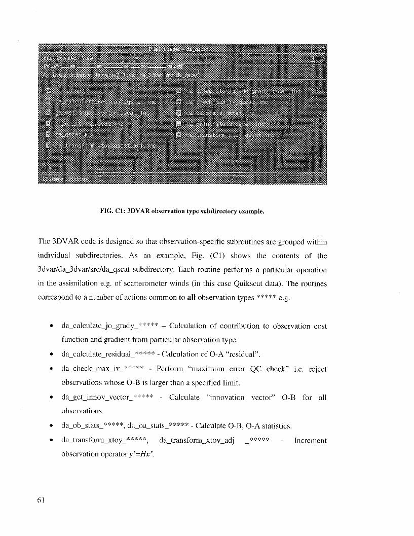
FIG. Cl: 3DVAR observation type subdirectory example.

The 3DVAR code is designed so that observation-specific subroutines are grouped within

individual subdirectories. As an example, Fig. (C1) shows the contents of the

3dvar/da_3dvar/src/da_qscat subdirectory. Each routine performs a particular operation

in the assimilation e.g. of scatterometer winds (in this case Quikscat data). The routines

correspond to a number of actions common to all observation types ***** e.g.

* da_calculatejo_grady_***** - Calculation of contribution to observation cost

function and gradient from particular observation type.

* dacalculateresidual ***** - Calculation of O-A "residual".

* da_check_max_iv_***** - Perform "maximum error QC check" i.e. reject

observations whose O-B is larger than a specified limit.

* da_get_innov_vector_***** - Calculate "innovation vector" O-B for all

observations.

* da_ob_stats_*****, da_oa_stats_***** - Calculate O-B, O-A statistics.

* da_transform_xtoy_** datrarnsform_xtoy_adj _*** - Increment

observation operator y'=Hx'.

61

In addition to these observation-specific routines, there are a number of areas of the code

that must be modified in order to assimilate a new observation type. The following

procedure has been tested as an algorithm to help in the introduction of a new observation

type "newob".

a) Copy existing observation-specific subdirectory (e.g. da_qscat above) to

"da_newob" subdirectory.

b) Rename and modify routines to act on variables of "newob" observation type.

c) Type "grep -ni qscat */*.* > change" in the da_3dvar/src directory to create a file

"change" that will contain all references to the string "qscat". This will indicate

the areas of the code that need modification. Known dependencies are

da_constants, da_define_structures, da_minimization, da_obs,

da_setup_structures, da_tools, da_test and par_util.

d) Create corresponding references for "newob" in code. This should provide all

necessary links to the code contained in the da_newob subdirectory.

e) Update src/Makefile to reflect the additional code and module dependencies.

f) Modify run script e.g. run/DA_Run_3DVAR.csh to reflect new options.

Once coded, standard initial tests include i) observation operator adjoint tests and ii)

single observation tests.

62

Appendix C - User Guide

a) Obtaining the MM5 3DVAR codes.

The 3DVAR web-site http:l/www.mmm.ucar.edu/3dvar contains links to the 3DVAR and

3DVAR observation preprocessor codes. In addition, there are links to documentation

e.g. this technical description and details of planned work and example results. A more

detailed user guide may also be found on the web site. The following is just an overview.

b) Compiling and running the 3DVAR preprocessor code.

To compile 3DVAR_OBSPROC, type "make" in the 3DVAR_OBSPROC top directory.

Successful compilation produces a 3dvar_obs.exe file in the current directory. To run

3DVAR_OBSPROC standalone, tailor the namelist file to include details of the

experiment and then type "3dvar_obs.exe".

c) Compiling and running the 3DVAR code.

In order to compile the code:

i. Extract the 3dvar code.

ii. cd to 3dvar directory.

iii. Type "configure" to automatically create the necessary compile options etc for the

platform you are running on.

iv. At the prompt, type "1" for serial code, "2" for the full distributed memory

platform capability. Compilation of the latter requires the MPI chameleon

(MPICH) library. This is available from http://www-

unix.mcs.anl.gov/mpi/mpich/. If you're not interested in MPP runs, type 1 - you

don't need MPICH, compilation is quicker and runtime CPU and memory are

significantly reduced.

63

v. Type "compile 3dvar".

Upon successful compilation, the file main/da_3dvar.exe is produced."

To run the code, edit the run/DA_Run_3DVAR.csh script to include links to your input

MM5 format background field, background errors and 3DVAR-format observation files.

An MM5-format background error file is available from the web-site. This has been

created using the "NMC-method" (see section 9) from forecasts of a near-global MM5

domain. Of course, these are only crude approximations to the true forecast errors of a

particular domain and should be treated as a starting point to test an application of

3DVAR. Benefits will almost certainly follow if attention is paid to tuning the default

background error statistics.

64

Appendix D - 3DVAR Namelist Parameters

The following is an example 3DVAR namelist file used as input to 3DVAR to define the

run-time configuration.

&recordlMODELTYPE = 'MM5',WRITEINCREMENTS = .FALSE. / ! If true, output large diagnostic increments file

&record2ANALYSISTYPE = '3D-VAR',ANALYSISDATE = '2002-09-12 12:00:00.0000', ! Analysis date. Note format.

ANALYSIS ACCU = 900 /

&record3fg_format = 2, ! 1 = WRF, 2 = MM5.

obformat = 2 / ! 1 = BUFR, 2 = MM5.

&record4PROCESSOBS = 'YES',

obs_qcpointer = 0,Use_SynopObs = .TRUE., ! Use_*****Obs = .false. switches obs off.

Use_ShipsObs = .TRUE.,UseMetarObs = .TRUE.,UsePilotObs = .TRUE.,UseSoundObs = .TRUE.,UseSatemObs = .TRUE.,

UseSatobObs = .TRUE.,Use_AirepObs = .TRUE.,Use_GpspwObs = .TRUE.,UseSsmiRetrievalObs = .FALSE.,

UseSsmiTbObs = .FALSE.,usessmtlobs = .FALSE.,usessmt2obs = .FALSE.,

use_qscatobs = .TRUE.,check max iv = .TRUE., ! If true, flag obs with O-B > threshold.

useobserrfac = .FALSE.,

put_rand_seed = .FALSE.,ombsetrand = .FALSE.,ombadd noise = .FALSE. /

&record5TIMEWINDOWPRINTDETAIL

&record6maxext itsEPSONTMAXNVERIFNSAVEWRITE SWITCHWRITE INTERVAL

&record7RFPASSESVARSCALING1VARSCALING2VARSCALING3VARSCALING4VARSCALING5LENSCALING1LEN SCALING2

= 3.,

= 0 /

= 1,

= 1.E-02, !

= 100,

= 0,

= 4,

= .FALSE.,

=5 /

6,

1.0,

1.0,

1.0,

1.0,

1.0,

1.0,

1.0,

Minimization terminates when gradient < epsO * initial value.Maximum number of minimization iterations.

Number of passes of recursive filter.

Factor to scale NMC-method background errors variances (psi).

Same for control variable 2 (chi)Same for control variable 2 (p_u)Same for control variable 2 (q/RH)Not usedNMC-method background errors lengthscales (psi) scaling.

Same for control variable 2 (chi)

65

LENSCALING3LEN SCALING4LEN SCALING5

= 1.0,

= 1.0,

= 1.0 /

! Same for control variable 3 (p_u)! Same for control variable 4 (q/RH)! Not used.

&record8NSMOOTH = 0,defsubdomain = .FALSE.,

xj_start_sub_domain = 55.0,yi_start_sub_domain = 35.0,xj_end_sub_domain = 80.0,yi_end_sub_domain = 60.0 /

&recordl0Testing_3DVAR = .FALSE.,TestTransforms = .FALSE.,TestStatistics = .FALSE.,Interpolate_Stats = .true /

&recordll

cv_options

cv_optionshum =checkrh =aslas2as3as4as5 =set omb rand fac

seedarrayl =seed_array2

&recordl2balance_type =

&recordl3vertcorr

vertical_ipvertevalue =maxvert varl =maxvert var2 =

maxvert var3 =maxvertvar4 =maxvert var5 =

&pseudoobnlnum_pseudo

pseudox =pseudo_y =pseudo_z =

pseudo_val =pseudo_errpseudovar =

2,

1, ! 1 = q as moisture control variable, 2= RH.

1, ! Perform check on physics limits of RH analysis.0.2,0.2,

0.5,0.5,0.5,= 1.0,

0,

0 /

1 /

2,

0,

1,

99.0,

99.0,

99.0,

99.0,

0.0 /

0,

1.0,

1.0,

1.0,

1.0,

1.0,

It' /

66

Appendix E - Example 3DVAR Output Files

Following successful minimization of the 3DVAR algorithm a number of output files are

produced as shown in Fig. 6. The analysis and analysis increments themselves are output

in MM5 format in files DAProg_3DVAR.analysis and DAProg_3DVAR.analincs

respectively. Files fort.35-fort.39 contain O-B data for each observation for variables u,

v, T, p and q that is accululated for later calculation of background/observation errors.

FIG. 6: Run directory following successful execution of 3DVAR program.

The two most useful output files are DAProg_3DVAR.out which contains run-time

observation, grid and minimization information and DAProg_3DVAR.statistics, which

contains O-B, O-A statistics for each observation type assimilated as well as minimum,

maximum, mean and RMS analysis increment statistics for u, v,, T, p and q broken down

by model level.

67

.. . ........... .......... ...----I

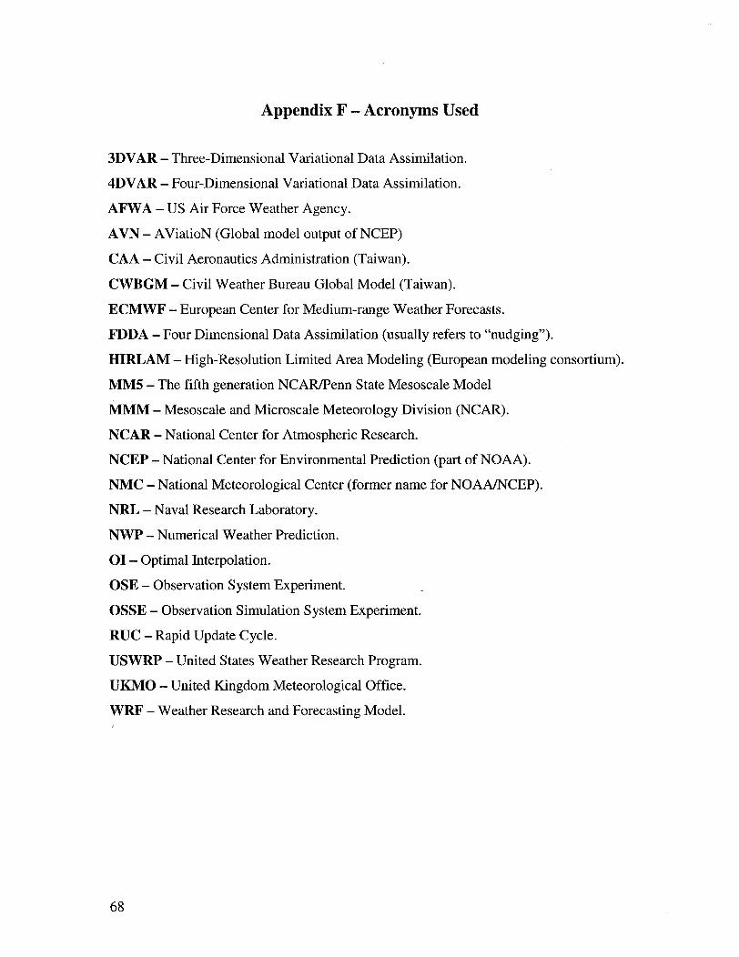
Appendix F - Acronyms Used

3DVAR - Three-Dimensional Variational Data Assimilation.

4DVAR - Four-Dimensional Variational Data Assimilation.

AFWA - US Air Force Weather Agency.

AVN - AViatioN (Global model output of NCEP)

CAA - Civil Aeronautics Administration (Taiwan).

CWBGM - Civil Weather Bureau Global Model (Taiwan).

ECMWF - European Center for Medium-range Weather Forecasts.

FDDA - Four Dimensional Data Assimilation (usually refers to "nudging").

HIRLAM - High-Resolution Limited Area Modeling (European modeling consortium).

MM5 - The fifth generation NCAR/Penn State Mesoscale Model

MMM - Mesoscale and Microscale Meteorology Division (NCAR).

NCAR - National Center for Atmospheric Research.

NCEP - National Center for Environmental Prediction (part of NOAA).

NMC - National Meteorological Center (former name for NOAA/NCEP).

NRL - Naval Research Laboratory.

NWP - Numerical Weather Prediction.

OI - Optimal Interpolation.

OSE - Observation System Experiment.

OSSE - Observation Simulation System Experiment.

RUC - Rapid Update Cycle.

USWRP - United States Weather Research Program.

UKMO - United Kingdom Meteorological Office.

WRF - Weather Research and Forecasting Model.

68