Technology Assimilation and Aggregate Productivity

Ping Wang, Washington University in St. Louis and NBERTsz-Nga Wong, Bank of Canada

Chong K. Yip, Chinese University of Hong Kong

December 2015

Abstract: This paper develops a technology assimilation framework to explain how do-mestic firms uncover global technologies under limited technique availability and productionflexibility. We construct a micro-founded measure of endogenous total factor productivity(TFP) based on the interaction of stage-dependent local knowledge of a country with ad-vanced foreign technologies. We then perform development and growth accounting exercisesto better understand the large and widening TFP gaps across countries and over time. Bycomparing our results with other popular models, we find that the success of assimilation offrontier technologies can be instrumental in differentiating miracle economies from trappedeconomies. About half of the rapid growth experienced in miracle economies can be at-tributed to successful assimilation, whereas about one third of the negative growth outcomein trapped economies is due to the lack of it or backward assimilation. This finding sug-gests that an adequate provision of correct incentives and institutional settings is crucial fordomestic firms to assimilate relevant frontier technologies in a way that is suitable for theirdevelopment stages.

JEL Classification: O41, O47, D90, E23.

Keywords: Assimilation of Global Technology, Flexible Production, Local Knowledge of Lim-ited Techniques, Development and Growth Accounting.

Acknowledgment: We are grateful for the valuable comments and suggestions of Fer-nando Alvarez, Costas Arkolakis, Paul Beaudry, Bob Becker, Rick Bond, Anton Braun, TomCooley, Peter Howitt, Boyan Jovanovic, Sam Kortum, Finn Kydland, Zheng Liu, SerdarOzkan, Steve Parente, Ed Prescott, B. Ravikumar, Ray Riezman, Victor Rios-Rull, PeterRuppert, Rob Tamura, Yin-Chi Wang, and Jianpo Xue, as well as those of the participantsat the North America Summer Meeting of the Econometric Society, the Asian Meeting ofthe Econometric Society, the Conference on Dynamics, Economic Growth, and InternationalTrade, the Midwest Macroeconomic Conference, the Society for Advanced Economic TheoryMeeting, Academia Sinica, and the National Taiwan University. We gratefully acknowledgethe financial support of Academia Sinica, Talent Strategy of the Bank of Canada, the ChineseUniversity of Hong Kong, and the Center for Economic Dynamics, that made this interna-tional collaboration possible. We would like to thank Terry Cheung and Ting-Wei Lai forhelpful research assistance. The usual disclaimers apply.

Correspondence: Ping Wang, Department of Economics, Washington University in St. Louis,Campus Box 1208, One Brookings Drive, St. Louis, MO 63130, U.S.A.; 314-935-4236(Phone); 314-935-4156 (Fax); pingwang@wustl.edu (E-mail).

“The sixteenth-century Dutch, on the verge of becoming economic leaders of

the world, borrowed heavily from the techniques of the Italians, the outgoing lead-

ers. By then, the English were already learning not only from the Low Countries

but also from other parts of the continent. The Americans borrowed heavily from

the English and from other European sources, particularly from the time they

achieved independence up until the middle of the nineteenth century.” (Baumol

et al. 1991 pp. 271-272)

1 Introduction

Why, in the past half-century, have many countries successfully taken off, catching up with

world leaders, while some have experienced growth stagnation? The world income distribu-

tion has widened over the last 50 years. From 1970 to 2011, the U.S. real GDP per capita

relative to that of poor nations in the bottom 10 percentile was about 5.4 times on average,

with the gap rising over time. Macroeconomists attempt to account for the income differences

using a neoclassical aggregate production function. They find that, even when controlling for

the accumulation of physical and (education-based) human capital per worker, an unusually

large total factor productivity (TFP) gap is still required to account for the income dispari-

ties (e.g., Lucas 2000). However, why would technology not flow from the rich to the poor?

Are there “missing inputs”in standard aggregate production? Are there “barriers to rich”in

less-developed countries? Over the past two decades, the field of development accounting has

emerged; it is devoted to understanding the underlying causes of the persistent and widening

world income disparities. These studies focus primarily on correcting the mismeasurements

of factors inputs and identifying missing inputs in the neoclassical production framework. In

this paper, we depart from neoclassical production theory to quantify endogenous TFP gaps

by examining country-specific processes of technology assimilation.

To illustrate our idea of technology assimilation in a nontechnical fashion, let us consider

a product (e.g., smartphones) with different product blueprints (such as Apple iPhone, Sam-

sung Galaxy Note, HTC One, etc.). In contrast to standard neoclassical production theory,

we generalize the concept of “production techniques” developed by Houthakker (1956-57),

Kortum (1997), and Jones (2005) to capture “mini-blueprints” that specify ways to orga-

nize factor inputs so that they fit a given product blueprint. In our framework, availability

of such production techniques is limited due to imperfect knowledge about product orders

1

ex ante and about the most effective mini-blueprints that are suitable for a particular firm

(e.g., Foxconn Technology Group). As a result, mismatches may arise and output can fall

below the potential level. In this circumstance, “production flexibility”can make firms less

vulnerable to their limitations in available techniques. In a global economy, a domestic firm

can “assimilate” a relevant global leader and thus expand its set of available techniques;

these assimilated techniques help to re-organize factor inputs in the continually changing

process of production. The endogenous choice of such techniques yields a dynamic process

of technology assimilation and generates endogenous TFP; however, this process depends on

“local knowledge”that summaries a country’s limitations related to the available techniques

and production flexibility. Which particular leader should be assimilated can also be differ-

ent across countries and over time. Assimilation under the condition of limited production

techniques and restricted flexibility can prohibit the flow of technologies from developed to

developing countries, leading to endogenous TFP gaps and the flying geese paradigm (FGP)

of economic development documented by Akamatsu (1962) and Baumol et al. (1991).

Numerous well-documented case studies show that successful assimilation of technology

is the common denominator in Asian economic development [Wan (2004)]. Geographical

proximity in technology assimilation generates the FGP, with some early birds taking off

sequentially, followed by various late comers. Conversely, failure to assimilate technology has

caused the backwardness seen in African economic development. In 1970, per capita incomes

of the Sub-Saharan countries were almost comparable with those of the Asian Tigers and were

even ahead of some of their ASEAN counterparts.1 Subsequently the Asian economies took off

and continued to advance along sustained growth paths, whereas Africa’s post-independence

industrialization remains isolated from world markets and frontier technologies, even in their

main sectors of production, such as cash crops (e.g., cocoa and coffee in Cote d’Ivoire and

Kenya).

As elaborated below, technology assimilation differs from the standard concepts of tech-

nology adoption, imitation, or spillover. In general, the ability of technology assimilation are

related to entrepreneurs’understanding of foreign techniques, their learning from experiment-

ing, the flexibility of institutions and organizations, the human capital that is responsive to

the frontier techniques, and the infrastructure and taxation schemes that enhance the adap-

1For instance, the 1970 per capita GDP of Korea and Taiwan was 16.1% and 15.6% that of the UnitedStates, and Thailand’s and Vietnam’s were only 9.2% and 3.9%, whereas there of Cote d’Ivoire and Kenyawere 12.6% and 8.4%, respectively.

2

tation. Thus, we can study how diverse growth experiences across countries can be explained

by this assimilation measure over time. To investigate the relationship between technological

advancement and flexible production, we need a systematic comparison between technologies

with different elasticities of substitution. We therefore adopt a constant elasticity of sub-

stitution (CES) production function normalized to a particular country at a given stage of

technology assimilation. We then decompose the real GDP per capita relative to the U.S.

(the income ratio) into a relative technology component (the TFP ratio), a relative factor en-

dowment component (the capital-labor ratio), and a time-varying, country-specific measure

of technology assimilation with respect to an advanced foreign technology, which depends on

the interaction of limited technique availability and production flexibility.

Our technology assimilation framework contributes to production theory and development

economics in several significant aspects. In contrast to the neoclassical production approach,

our framework disentangles the designed usages of production factors (production techniques)

for a given level of technology from the physical inputs of production factors. Because the

mini-blueprints governing factor use are specific to each production input, our framework is

also different from organizational capital theory. Accordingly, we are able to establish a clear-

cut relationship between technological advancement and production flexibility. Moreover, by

comparing local performance and global technology, we can extract more information from

the data and can obtain measures of production flexibility and technology assimilation that

are specific to a country over time. This allows us to generate new measures of TFP. We

thus gain further insights into the role of assimilation in the dynamic process of economic

advancement for various countries, and obtain new measures of aggregate productivity that

are sharply different than comparable figures computed under the conventional neoclassical

production framework. As our model is related to the literature of appropriate technology,

we perform income accounting exercises and systematically compare them with other popular

models such as those given in Lucas (2000), Basu and Weil (1998), and Acemoglu (2009).

We shall refer to the Basu-Weil-Acemoglu framework of inappropriate technology as BWA

because of its high relevance. We also generalize the Cobb-Douglas benchmark of Lucas

(2000) with the CES formulation, referred to this generalization as the CES model.

The main findings of this paper are as follows. Theoretically, when local information

about the available techniques suitable for domestic use is limited, the technologies will not

flow from more advanced to less advanced countries. Poor assimilation is the barrier to

growth and leaves nations in poverty traps. Using the normalized CES specification for the

3

assimilation process, we decompose the aggregate production function into two components:

a conventional Cobb-Douglas production term and a CES-type assimilation term. We show

that country-specific assimilation of a global technology can serve as an effective vehicle for

development accounting and can help to reduce the unexplained component in the large TFP

differences.

Quantitatively, our development accounting results suggest that our model of the assim-

ilation of global technology, the CES and the BWA models fit the data far better than the

Lucas benchmark. Moreover, our model, on average, outperforms both the CES and the BWA

models in most economic and geographic groups (classified by initial stage of development,

development speed, and current state of development). These advantages are particularly

noticeable for countries that are either in development traps or are experiencing development

miracles. Furthermore, we select a group of representative countries and separate them into

the following economic/geographic clusters: OECD, Asian Miracles, late-coming miracles,

trapped, and laggards. By conducting growth accounting exercises, we find that the Lucas

benchmark performs well for OECD countries, but noticeable differences exist between our

model and the CES and the BWA models for trapped and miracle countries. Specifically,

more than half of the relative income growth in all of the miracle countries can be attributed

to successful assimilation. Moreover, the lack of or backward assimilation accounts for about

one third of the negative growth performance of all of the trapped countries. By backward

assimilation, we refer to the situation where assimilating a foreign frontier leads to lower

production performance. Most of the development miracles have exhibited successful assimi-

lation over the past four decades, whereas many of the trapped economies are found to suffer

from the lack of or backward assimilation. Therefore, we can conclude that the effective

assimilation of frontier global technology is an important factor for explaining many of the

Asian Miracle cases, and the lack of assimilation of frontier global technology is crucial for

explaining why most Sub-Saharan African countries suffer the poverty trap. Moreover, we

identify successful assimilation with the flexibility of production over time, and find that

the two larger Asian Tigers (i.e., South Korea and Taiwan) are more flexible in (techniques-

augmented) factor substitution than the two smaller Tigers and that India (software-led) is

more flexible than China (assembly-based). Such flexibility has important implications for a

country’s production effi ciency and development success.

Finally, based on country-specific growth data, we find that the fitness of our assimilation

model significantly improves when we allow for delayed assimilation in several Latin American

4

countries and an early stop of assimilation in Hong Kong and Singapore. Allowing Taiwan

to first assimilate the techniques from Japan and then from the U.S. yields a much better fit;

a similar assimilation switching does not change the results for Korea. For several ASEAN

economies and China, geographical or FDI-based assimilation gives much better model fitness

outcomes. In contrast, no alternative assimilation schemes improve the fitness outcomes for

most of the trapped economies where technology assimilation is found lacking or backward.

Related Literature

Our paper is related to two strands of research: the study of appropriate technology and

the study of development accounting.

To formalize the concepts of technology assimilation, we refer to the now-classic pieces by

Atkinson and Stiglitz (1969) and Houthakker (1956-57) and more recent studies by Kortum

(1997) and Jones (2005). Atkinson and Stiglitz specify that a country’s local production

features localized learning by doing. Houthakker, Kortum, and Jones obtain a Cobb-Douglas

production function as an envelope of Leontief local productions in which firms are free to

choose any production techniques drawn from independent Pareto distributions. Based on

the idea of local production, Basu and Weil (1998) construct a Solow-type growth model of

technological progress that emphasizes that technological advances will benefit certain types

of technologies, but not others. Therefore, even if all technologies are freely available and

instantly transferred, a country may refrain from using a new but “inappropriate”technology.

Parente and Prescott (1994) examine how barriers to technology adoption affect the process

of development. With the exogenous growth of world knowledge, the amount of investment

required for technological advances decreases, and this enhances long-term growth. Recent

studies have focused on costly technology acquisition, including Caselli’s (1999) study of costly

learning. Caselli and Coleman (2006) show that given different economic conditions and

factor endowments, some countries may optimally choose not to adopt a frontier technology.

Acemoglu (2009) provides a heuristic Leontief specification of the Basu-Weil appropriate

technology so that the production function is Cobb-Douglas and the appropriateness can be

summarized by a single parameter defined on the unit interval. Depending on the magnitude

of this parameter, the latter study shows that the inappropriateness of some technologies

has the potential to explain cross-country income differences. Building on the Houthakker-

Kortum-Jones foundation, Wong and Yip (2014) construct a model of technology assimilation

to study how adopting a frontier technology may lead to a development trap instead.

5

Since the pivotal works of Lucas (1990, 2000), Chari, Kehoe, and McGrattan (1996),

and Prescott (1998), there has been a growing interest in development accounting. Many

contributions have attempted to reduce the required TFP gap by improving the measurements

of the quality of physical and human capital and the associated barriers and distortions.

To name a few, Caselli and Wilson (2004) introduce “quality” of physical capital in the

accounting exercise. Erosa, Koreshkova, and Restuccia (2010) and Schoellman (2012) improve

the measurement of human capital beyond the typical Mincerian ‘years of schooling’estimate.

Aghion, Howitt, and Mayer-Foulkes (2005), and Buera and Shin (2012) study the role of

financial markets distortions on capital investment to account for world income disparities.

2 The Aggregate Production Function: A Prelude

In order to understand the cross-country variation of the aggregate production function, the

existing literature adopt the prototypical model

yj =YjNj

=zjF (Kj , Nj)

Nj= zjf (kj) . (1)

According to (1), a representative firm in country j employs capital K and labor N to

manufacture a final product Y using a constant-returns-to-scale technology with total factor

productivity (TFP) z. In per capital term, we have k = K/N and f(k) = F (k, 1). The

standard practice is to allow the TFP (z) to vary across countries so that z is higher in

high-income countries. Lucas (2000) focuses on the Cobb-Douglas specification of F :

yLucasj = zLucasj kαj , (2)

where α ∈ (0, 1) is the common output elasticity of capital for all countries. Based on (2),

the common conclusion is that about 40% of the variation in world income can be attributed

to differences in z. However, TFP is a residual component which measures our ignorance of

the production relation specified in f . So recent research attempts to study extensions to the

aggregate production function in order to reduce the resulting z.2 Our model of technology

assimilation follows this line of research. In the assimilation framework studied in the next

section, we extend the aggregate production function by allowing a country to adopt an

advanced (more capital intensive) foreign technology for its domestic production along the

line proposed by Houthakker (1955-56) and Jones (2005). The assimilation between the

2The literature on TFP is huge and we refer the readers to Caselli (2005) for a partial survey.

6

foreign technology and the domestic factor endowment in the adoption process is shown to be

captured by an elasticity of substitution to reflect the flexibility of the aggregate production

function. Specifically, we can establish the resulting micro-founded per worker aggregate

production function of the form:

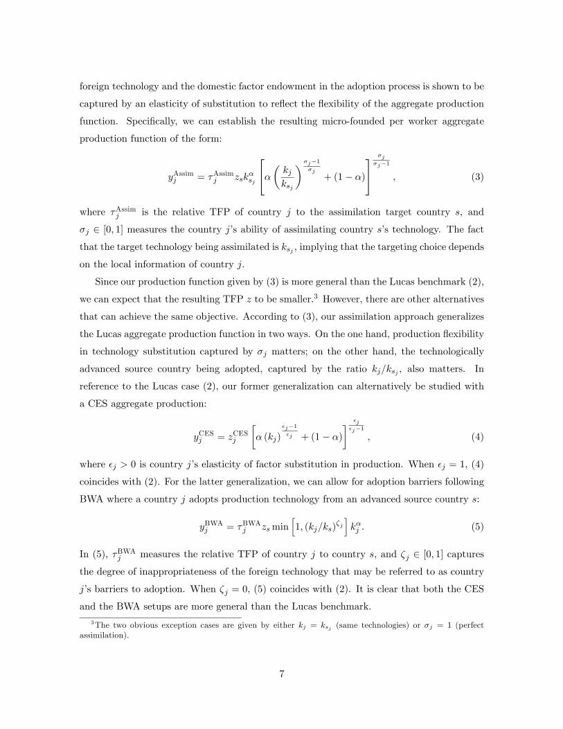
yAssimj = τAssimj zskαsj

α( kjksj

)σj−1σj

+ (1− α)

σjσj−1

, (3)

where τAssimj is the relative TFP of country j to the assimilation target country s, and

σj ∈ [0, 1] measures the country j’s ability of assimilating country s’s technology. The fact

that the target technology being assimilated is ksj , implying that the targeting choice depends

on the local information of country j.

Since our production function given by (3) is more general than the Lucas benchmark (2),

we can expect that the resulting TFP z to be smaller.3 However, there are other alternatives

that can achieve the same objective. According to (3), our assimilation approach generalizes

the Lucas aggregate production function in two ways. On the one hand, production flexibility

in technology substitution captured by σj matters; on the other hand, the technologically

advanced source country being adopted, captured by the ratio kj/ksj , also matters. In

reference to the Lucas case (2), our former generalization can alternatively be studied with

a CES aggregate production:

yCESj = zCESj

[α (kj)

εj−1εj + (1− α)

] εjεj−1

, (4)

where εj > 0 is country j’s elasticity of factor substitution in production. When εj = 1, (4)

coincides with (2). For the latter generalization, we can allow for adoption barriers following

BWA where a country j adopts production technology from an advanced source country s:

yBWAj = τBWAj zs min[1, (kj/ks)

ζj]kαj . (5)

In (5), τBWAj measures the relative TFP of country j to country s, and ζj ∈ [0, 1] captures

the degree of inappropriateness of the foreign technology that may be referred to as country

j’s barriers to adoption. When ζj = 0, (5) coincides with (2). It is clear that both the CES

and the BWA setups are more general than the Lucas benchmark.

3The two obvious exception cases are given by either kj = ksj (same technologies) or σj = 1 (perfectassimilation).

7

While our framework is more general than the Lucas benchmark, the comparison with the

CES and the BWA setups is not straightforward. On the one hand, production flexibility in

factor substitution matters, similar to the CES setup but in contrast to the BWA setup. On

the other hand, the advanced source country matters, similar to the BWA approach but in

contrast to the CES setup. Moreover, in contrast to both setups, how to assimilate the target

country s’s technology captured by both the ratio kj/ksj and σj is crucial. Specifically, the

target country for assimilation depends on the "local" conditions of country j, as highlighed

by the notation ksj instead of ks, which does not necessarily have to be the world technology

frontier. In order to provide a better understanding on these issues, we now turn to study

the microfoundation of the underlying assimilation mechanism.

3 The Model

Consider a production environment in which a firm specializes in a particular product that

has a range of product blueprints, that vary between orders. Departing from the neoclassical

production framework, we introduce the concept of “production technique,”which is a mini-

blueprint that specifies how to organize factor inputs to fit a given blueprint. Before a

particular order specifies a blueprint, the factor inputs have already been employed by the

firm. Together with imperfect knowledge about the potentially most effective component

design, these ‘pre-determined’ inputs may limit the available choices of techniques. If the

available techniques are limited, the firm’s optimization problem can produce an outcome

that differs sharply from the neoclassical one.4 In particular, not only does the set of available

techniques matter, but the “flexibility”of production under limited alternatives is also crucial.

Given a limited set of available techniques, which may not be perfectly suited to the factor

endowment of the firm, output can fall below the potential level. Flexibility of production is

the ability to relieve the tension between limited alternatives and a pre-set factor endowment

so as to reduce the output loss from its potential level. In other words, a more flexible pro-

duction makes the firm less vulnerable to its limitations in available techniques. We describe

the firm’s flexible organization of production inputs as “technology assimilation,”which can

be understood as a process of alternating a mini-blueprint under its factor endowment. No-

tably, assimilation differs from Lucas’ (1978) span-of-control theory of production, which

augments neoclassical production with an additional managerial input. Instead, assimilation

4This captures the spirit of the local production function described in Atkinson and Stiglitz (1969).

8

re-organizes factor inputs in the process of production, generating flexible mini-blueprints

that we refer to as “assimilated techniques.”The firm then chooses and implements the most

suitable assimilated technique for production, aiming to reduce effi ciency losses caused by

limitations in available techniques.

Limitations in available techniques and production flexibility under assimilation are im-

portant components of a firm’s “local knowledge.” In a global economy, domestic firms are

given opportunities to assimilate relevant techniques from global leaders. This advanced

technique expands the set of available techniques and the local knowledge of domestic firms,

initiating an assimilation process. We can then account for the output gap between a country

and the global leader, the so-called TFP difference, based on the dynamic interaction of a

country’s local knowledge with advanced foreign techniques. As a result, we have a theory

of endogenous TFP based on technology assimilation.

Using the concepts of modified production under assimilation and cross-country variations

in local knowledge, we establish a new development accounting framework for generating

insights into the large and widening TFP gaps across countries and over time.

3.1 Production Technique

A production technique is a mini-blueprint that specifies the organization of factor inputs,

capital (K), and labor (N), for an output level Yi, defined by two parameters of factor-

augmented productivity, ai and bi.5 Thus,

Yi = min(aiK, biN) = Nbi min(k

κi, 1), (6)

where k ≡ K/N and κi ≡ bi/ai. That is, technique i is indexed by (bi, κi) ∈ P, where themenu P is the set of techniques. The capital-labor ratio k is what matters to the output percapita because of constant return to scale. We want to emphasize that κi is the input required

by the technique i, and k/κi measures the mismatch between the factor endowment ratio and

technique requirement. This mismatch is due to the limitation in available techniques, which

prevents choosing κi = k. When κi > k, capital is insuffi cient to achieve the potential output

κi = k; when κi < k, some capital is wasted.

For choosing a technique, k is given and κi is the subject of selection. Given k, the

firm would like to match the technique perfectly to the capital-labor ratio such that κi = k.

5See Houthakker (1956-57), Kortum (1997), and Jones (2005) for further details of this Leontief formulationof the so-called local production.

9

But it may not be feasible, as the menu P only consists of a limited number of techniques.The concept of production techniques can be best illustrated using a two-sided matching

terminology, as outlined in Chen, Mo, and Wang (2012). Technique i′ is called latent if

bi′ < bi for κi′ = κi or κi′ > κi for bi′ = bi. A latent technique yields a lower output per

worker given the same input requirement or requires more input to yield the same output

per worker. We shall call a technique manifest if it is not latent. Then we denote the

set of manifest techniques as B, and define the manifest technique associated with κ as

B (κ)≡{bi|bi = max(bj ,κ)∈P bj

}∈ B, which is the best technique for a given κ in a country.

It is important to note that P, and hence B, can be different across countries and time.

3.2 Assimilated Technique and Production

We are now prepared to introduce the concept of technology assimilation. Recall that the

menu P may consist of a limited number of techniques. As a result, we may have a mismatch,and output may fall below the potential level. Technology assimilation is a means to mitigate

the detrimental consequence of a mismatch by allowing for alternative ways of organizing

techniques with respect to the factor endowment. To capture this, we propose the following

production function under assimilation, which specifies the output with the technique (ai, bi),

given the factor endowment (K,N) such that

F (K,N ; ai, bi) = τ[α (aiK)

σ−1σ + (1− α) (biN)

σ−1σ

] σσ−1

. (7)

It is clear that when (ai, bi) = (z, z), F (K,N ; z, z) becomes a standard neoclassical CES pro-

duction function with TFP captured by τz. When (ai, bi) = (a, b), i.e., the set of techniques

is a singleton, F (K,N ; a, b) capture the production technology with factor-biased technical

progress as in Acemoglu (2003).

Our production function under assimilation is not a simple extension of neoclassical pro-

duction. As in the neoclassical framework, τ is an effi ciency measure, though it is now

specific to the implementation of a particular technique for production. In sharp contrast to

the neoclassical framework, we consider the endogenous choice of production technique, and

introduce technology assimilation that depends crucially on the limited menu of available

techniques and the flexibility parameter σ ∈ [0, 1]. In particular, although limitations in

available techniques can result in mismatches, assimilation under greater flexibility (higher

σ) can help to mitigate the output loss caused by these mismatches. As analyzed below, the

endogenous choice of a manifest technique under a limited menu of techniques will generate

10

new measures of TFP, that depend jointly on technique limitation and flexibility.It is con-

venient to rewrite the production function in terms of an assimilated technique (bi, κi) ∈ Psuch that

F (K,N ; bi, κi) = τbi

[α

(K

κi

)σ−1σ

+ (1− α)Nσ−1σ

] σσ−1

. (8)

This turns out to be the normalized CES production function proposed by Klump and de la

Grandville (2000), where the normalization point is specified at the input requirement of a

technique target, κi. A graphical representation of the assimilation concept is given in Chart

1. Consider a menu consisting of two available techniques, κ1 and κ2. In the case where

σ → 1, we have perfect assimilation and F becomes Cobb-Douglas, and the potential output

y3 is achieved. In the case where σ → 0, it is impossible to assimilate the technique and F

is Leontief. The output under technique κ1 is then given by y1 < y3. With σ ∈ (0, 1), we

have partial assimilation. Under technique κ1, output becomes y2 ∈ (y1, y3); under κ2, the

potential output y3 can be achieved, but some capital is wasted.

Given the capital rental rate r and the wage rate w, the profit maximization problem of

a representative firm can be conveniently specified in two steps. In the first step, for any

manifest technique κ, the associated output is F (K,N ;B (κ) , κ) and the resulting profit is

π (κ; r, w) = maxK,N{F (K,N ;B (κ) , κ)− rK − wN} , (9)

which is the standard neoclassical firm’s optimization problem. In the second step, for

(B (κ) , κ) ∈ P, the optimization problem becomes

Π (r, w) = maxκ{π (κ; r, w)} . (10)

The solution to the two-step optimization problem then gives the global production function

of Jones (2005). It can be shown that it is given by (see Appendix A)

F (K,N) = zKαN1−α, (11)

where z is a positive constant. In summary, the global frontier of a country with a universe

menu U ≡ {(b, κ) |b ≤ zκα} has the Cobb-Douglas functional form given in (11).

Chart 2 provides a graphical representation of π (κ; r, w). It is clear that π (κ; r, w) is

peaked at κ = k. When factor prices are high and production effi ciency is low, π (κ; r, w) can

be negative for a κ far away from k. Chat 1 depicts the local and global production under

11

only two available techniques, κ1 and κ2, both are different from k. As shown in Chart 2,

both techniques are inferior to k. Although κ2 is able to achieve the potential output y3, it

is not necessarily more profitable than κ1. This is because if capital is very expensive (high

r), the wasted capital can be costly enough to outweigh the extra output produced.

For a given production technique κ, we have σ = −d ln (k/κ) /d ln (r/w). In the limit case

σ → 0, the mismatch k/κ is not responsive to changes in the relative factor price, r/w. In the

case of σ → 1, the assimilation is so flexible that the unit cost always remains constant no

matter how r/w changes. A country’s local knowledge consists of a triple {P, σ, τ}. If eitherP is the universe menu U , or σ = 1, we have the Cobb-Douglas global production function.

In this case, τ is just the conventional TFP measure. In general, the other two components

of local knowledge P and σ will change the TFP measure.To apply the assimilation model for understanding world income differences, we suppose

that firms can assimilate the manifest technique (b, κ) of an advanced foreign global frontier,

where b = zκα. As a result, the menu P ⊂ U is augmented by additional techniques fromthe global frontier aboard. Specifically, the assimilation process simply recovers one point

of the foreign global production function, represented by the technique associated with κ.

If the assimilation is perfect so that the domestic country recovers the whole global frontier

production function, then we have σ → 1 and τ = 1. Therefore, the TFP wedge parameter τ

measures the productivity difference after the assimilation process, with a higher τ indicating

less productivity loss after the assimilation.

3.2.1 Production Flexibility: A Remark

Just how production flexibility from assimilation may affect production effi ciency? We would

like to refer to a recent work by Uras and Wang (2014), who show that, given the techniques

constraint aψi b1−ψi = z, techniques ratio and factor inputs ratio are inversely related:

aibi

=

(α

1− α

) σ1−σ (w

r

) σ1−σ

(K

N

)− 11−σ

Moreover, the unit cost of production can be solved as:

c(w, r) =1

z

((ψ

α

) σσ−1 r

ψ

)ψ ((1− ψ1− α

) σσ−1 w

1− ψ

)1−ψIn the limit cases with extreme flexibility measures, the unit cost of production converges

to: (i) σ → 0: c(w, r) = 1z

(rψ

)ψ (w1−ψ

)1−ψ; (ii) σ → ∞: c(w, r) = 1

z

(rα

)ψ ( w1−α

)1−ψ. Thus,

12

while factor prices are always weighted by the technique usage share (ψ), how much they

affect the unit cost depend crucially on production flexibility. When flexibility is shut down

(σ → 0), the production technology (the CES aggregator) precludes technique-augmented

factor inputs from substituting by each other. So factor prices are deflated only by their

technique usage shares. With a greater technique usage share, a factor price would not raise

the unit cost of production as much. When flexibility is perfect, on the contrary, factor prices

are deflated only by their income shares. In this case, an increase in the price of a factor with

a greater income share would become less damaging to the unit cost of production.

Using the expressions above, one may obtain:

yAssimj = (1− α)σjσj−1 τAssimj bi

(1 +

r

wkj

) σjσj−1 (12)

where r and w are capital rental and labor wage, τAssimj measuring the relative TFP of country

j to the assimilation target country s, and bi is a specific labor-augmented technique used by

country j. Thus, from (12), the variance of output per worker of country j (yAssimj ) can be

decomposed into three sub-components: the variance of the factor income ratio (rkj/w), the

variance of labor-augmented technique (bi) and the variance of TFP (τAssimj ).

Importantly, following the logics underlying Chart 1 and the optimization specified in

Π (r, w) = maxκ {π (κ; r, w)}, assimilation of a global technology is now embedded in the

parameter σj that entails the extent to which such an assimilation can be done effectively.

More specifically, by applying Uras and Wang (2014) with σ ∈ (0, 1), production flexibility

(σj) can be shown to monotonically reduce the unit cost of production for any given pair of

factor prices (w, r). This implies a positive impact of production flexibility on production

outcomes. That is, greater flexibility in a country is, other things being equal, expected to

be associated with a smaller TFP gap from the frontier economy.

3.3 Assimilation of a Global Frontier

We define the global frontier as the country with a universe menu U , where the productionfunction has the Cobb-Douglas functional form, as shown in the previous section. Suppose

that firms can assimilate the manifest technique (b, κ) of the global frontier, where b =

zκα. As a result, the menu P ⊂ U is augmented by additional techniques from the global

frontier. Specifically, the assimilation process of global technology simply recovers one point

of the global frontier production function, represented by the technique associated with κ.

If the assimilation is perfect so that the domestic country recovers the whole global frontier

13

production function, then we have σ → 1 and τ = 1. Therefore, the TFP wedge parameter τ

measures the productivity difference after the assimilation process, with a higher τ indicating

less productivity loss after the assimilation.

From (8), we can formulate an endogenous TFP using the global frontier technique:

z

(k

κ, σ, τ

)≡ Fκ(k, 1)

kα= τz︸︷︷︸TFP effect

×(κk

)α [α

(k

κ

)σ−1σ

+ 1− α] σσ−1

︸ ︷︷ ︸assimilation effect

. (13)

When a country assimilates the frontier technique (b, κ), its TFP measure, z(kκ , σ, τ

), be-

comes endogenous and contains two effects: (i) a conventional TFP effect, captured by τ ; and

(ii) an assimilation effect, jointly captured by the assimilation parameter σ and the mismatch

or capital waste k/κ depending on the limitation on P. Clearly, adopting and assimilatingthe frontier technique may not always lead to a higher TFP than autarky. As the assimilation

ability of a country decreases (thus σ decreases), the endogenous TFP measured by z also

decreases. Moreover, the endogenous TFP is lower when the factor endowment is further

away from the input required by the advanced foreign technique (i.e., |k − κ| increases).6

Interestingly, in the case of perfect assimilation, σ → 1 and z = τz; this is the exam-

ple used by Lucas (2000) for development accounting. In contrast, the extreme case of no

assimilation, i.e., σ → 0 and z = τz (k/κ)1−α, becomes a special case of BWA.

It is noteworthy that, throughout our analysis, we have used the country-specific representative-

producer setup that is typically used in development accounting, including in our main ref-

erence points, in Lucas and in BWA. For completeness, however, we would like to provide a

brief discussion on what happens if firms within a country are heterogeneous. Let us main-

tain the assumption that the share parameter α is global and the elasticity parameter σ is

country-specific but common to all domestic firms. However, firms may have different menus

of techniques and different endowment ratios, that is, k/κ may be firm-specific. From (13),

the term capturing the assimilation effect is hump-shaped in k/κ, reaching the maximum

of one at k/κ = 1. It is strictly concave for k/κ < 1 and turns from strictly concave to

strictly convex when k/κ becomes suffi ciently larger than one. Suppose that all firms have a

menu with k/κ < 1, and therefore suffer mismatch losses. Then, by Jensen’s inequality, the

average of the assimilation effects associated with all of the different firms is smaller than

the assimilation effect associated with the average (representative) firm. In this case, the

6 It is straightforward to show that ∂z/∂σ > 0 and ∂z/∂ (k/κ) > 0 iff k < κ.

14

assimilation effects become weaker when they are aggregated over heterogeneous firms. In

contrast, suppose that all of the firms have values of k/κ that far exceed one, with severe

capital waste. Then the average of the assimilation effects associated with all of the firms

is larger than the assimilation effect associated with the average firm, implying stronger as-

similation effects in the presence of firm heterogeneity. In general, the conclusion becomes

ambiguous; nonetheless, the gap between heterogeneous and representative firms tends to

narrow as σ increases. That is, the distributional effects from firm heterogeneity become

smaller under greater production flexibility. When heterogeneous firms are free to choose

any production techniques drawn from independent Pareto distributions, we have the Cobb-

Douglas production function as in Houthakker (1956-57), Kortum (1997), and Jones (2005)

and the accounting exercise reduces to Lucas (2000).

4 Development Accounting

Suppose that the reference country, the U.S., is on the frontier of technology (i.e., having the

collection of the highest a and b). So the U.S. uses its own domestic technology and does

not adopt any foreign technique. The US output is yUS,t = zUS,tkαUS,t. We allow the US

productivity and per capita capital to change over time, as denoted by the time subscript t.

Beside Lucas (2000), our specification of technology assimilation is also related to the

concept of localized technological changes proposed by Atkinson and Stiglitz (1969). Re-

cently, Basu and Weil (1998) elaborate on this idea of inappropriate technology in the Solow

growth model, where appropriateness is defined in terms of capital intensity: a technology

is appropriate for one and only one capital-labor ratio. The intuition is that frontier tech-

nologies are generally designed in reference to a specific capital intensity. For instance, if the

technology is developed for high-capital-intensive production in advanced economies, then

adopting it is not appropriate for developing countries because the production taking place

in developing countries is usually high-labor intensive. We compare our assimilation model

with Lucas (2000) and Basu and Weil (1998). Finally, given that our production function

under assimilation takes a CES specification, we also study a version of Lucas (2000) where

output are produced with standard CES technologies in all countries.

The Assimilation Model. If the US technique is assimilated, the relative income qj,t of

15

country j to the frontier captured by the U.S. in year t is

qj,t ≡fj(kj,t; kUS,t, zUS,t, τ

Assimj , σj)

yUS,t= τAssimj

α( kj,tkUS,t

)σj−1σj

+ (1− α)

σjσj−1

. (14)

Note that we now allow the TFP distortion parameter τ j and the assimilation parameter σj

to be country specific, and they will be investigated by the development accounting exercise.

The relative capital-labor ratio kj,t/kUS,t in the relative income expression above must be

recognized as a techniques-augmented factor proportion: the effective factor of the country

j in terms of the input required by the US technique. The decisions on assimilated foreign

techniques and optimized factor demands are made jointly. This techniques-augmented factor

proportion and the elasticity of substitution between the two techniques-augmented factor

inputs capture the process of technology assimilation. One should not view our techniques-

augmented factor proportion as one that simply measures the capital accumulation effect

relative to the frontier because of its different meaning from the conventional literature.

The Lucas Model. In this case, countries produce output according to their domestic

production functions so that the income ratio becomes

qj,t ≡fj(kj,t; kUS,t, zUS,t, τ

Lucasj , 1)

yUS,t= τLucasj

(kj,tkUS,t

)α. (15)

Note that the calibration exercise based on (14) has Lucas (2000) as a special case of σ = 1.

We denote τLucasj as the corresponding TFP distortion parameter in the Lucas model.

The CES Model. To allow for more flexibility into the Lucas benchmark, suppose that all

countries’output are given by the standard CES production functions:

yj,t = zj,t

[α (kj,t)

εj−1εj + 1− α

] εjεj−1

.

In order to compare with the BWA and assimilation models, we apply the idea of normalized

CES technique to the US economy so that εUS = 1 and hence yUS = zUS (kUS)α. Since

normalization per se does not have any implications on technology adoption, we do not

impose any restriction on the parameterization of εj . Thus, the resulting εj can take on

values that are either greater or less than unity. The relative income is given by

qj,t ≡fj(kj,t; kUS,t, zUS,t, τ

CESj , εj)

yUS,t= τCESj (kUS,t)

−α[α (kj,t)

εj−1εj + 1− α

] εjεj−1

. (16)

16

Again, note that the Lucas case is a special case of the CES model, where εj = 0.

The BWAModel. To compare the concept of inappropriate technology with our assimilated

technology, we follow the specification of Acemoglu (2009) to have the following intensive

production function of country j:

f(kj , ks) = τBWAj zs min

[1, (kj/ks)

ζj]

(kj/ks) kαj , (17)

where ks is the level of foreign capital designed for the technology with TFP zs in the source

country s, and ζj ∈ [0, 1] captures the degree of inappropriateness of the foreign technology.

As ζj increases, the inappropriateness increases so that the productivity of the adopted

technology and thus the domestic production is reduced. Again the TFP wedge parameter

τBWAj captures the net effi ciency in overall production after the adoption of the inappropriate

technology. Setting the U.S. as the source country implies that the per capita income ratio

of country j relative to that of the U.S. is

qj,t ≡fj(kj,t; kUS,t, zUS,t, τ

BWAj , ζj)

yUS,t= τBWA

j

(kj,tkUS,t

)α+ζj. (18)

We will compare the calibration and development accounting results between the BWA model

and our assimilation model. Again, note that the Lucas case is a special case of the BWA

model, where ζj = 0.

4.1 Data, Parameterization, and Methodology

We use the Penn World Table 8.0 (PWT) over the period of 1970 to 2011.7 The first 10 years

of the data (1960 to 1969) are discarded to calculate the initial level of capital as in standard

real business cycle exercises. We exclude former USSR countries (data do not start in 1970)

and all OPEC countries (due to nonstandard economic responses similar to the concern with

the financial tsunami). For China, we use the Version 2 data. In the end, we have a panel of

151 countries over a time span of 38 years.

Following Hall and Jones (1999), we set α = 1/3 and 6% as the depreciation rate of

capital to calculate the level of capital from the investment data in PWT. Bearing in mind

the potential endogeneity problem when recovering parameters from the data of output and

capital, we calibrate the TFP wedge parameter τ i and the assimilation parameter σi to match

the average level of log (qi,t) and the average lag difference of log qi,t (thus matching the long-

7We use PWT 6.3 for the sake of robustness. See Johnson et al. (2013) for concerns about the reliabilityof the versions of PWT after 6.3.

17

run income gap with respect to the US and the long-run growth rate of the income gap).

Similarly, we calibrate the productivity ratio τ i and the inappropriateness parameter ζi of the

BWA model to match the average level of log (qi,t) and the average lag difference of log qi,t.

The Lucas model only has one free parameter, and we calibrate the productivity ratio τ i to

match the average level of log (qi,t). (See Appendix B for detailed calibration steps)

Conventionally, for development accounting, fitness is measured by the success rate:

S =var(explained component of log(income ratio))

var(log(income ratio)).

Note that this measure crucially depends on the magnitude of the variance of the explained

component of log(income ratio), which cannot reflect any bias in the explained component.

For example, consider log y = β + log y, where β 6= 0. Then, we have S (y) = 1 = S (y); i.e.,

y and y are equivalently good fit to y. To rectify this problem, we propose a mean squared

error (MSE) measure over the period of interest t = 1, ..., T :

MSE ≡

√√√√ 1

T

T∑t=1

[errort]2 . (19)

Specifically, MSE captures the income ratio that cannot be captured by the explained com-

ponent. Although MSE is not a normalized measure and can be greater than one, it is a

measure that will not suffer the bias problem mentioned above. Therefore, we shall use the

MSE measure as the criterion to judge the fitness of the model.8

4.2 Results

The average of our calibrated values of the productivity ratio τ j and the assimilation pa-

rameter σj are reported in Table 1. The average values are based on various groupings of

countries: (i) initial stage of development measured by the income ratio (real GDP per capita

relative to that of the U.S.) in 1970 (< 10%, 10%− 20%, 20%− 50%, and > 50%); (ii) speed

of development measured by the average growth rate from 1970 to 2011 (< 0%, 0% − 1%,

1% − 2%, 2% − 4%, and > 4%); (iii) current state of development measured by the income

ratio in 2011 (< 20%, 20%− 40%, 40%− 60%, 60%− 80%, and > 80%). As an illustration,

Figure 1a (1b) plots the MSEs of the BWA (CES) model and our assimilation model based

on different country groupings of their average growth rates. We have adjusted the number

of categories from five to four by combining the first two groupings (< 0% and 0%− 1%) for

8For a comparison between S and MSE of the models, see Figure A1 in the appendix.

18

better graphical display.9

The results suggest that the fitness of our assimilation model based on our constructed

MSE measure is very good: the averaged value of our MSE measure in all different groups

ranges from 0.09 to 0.21. Interestingly, the best fitness is obtained for countries experiencing

moderate to fastest growth (MSE = 0.09 for those growing at a rate between 2% and 4%

annually) or for those in the upper-middle income group (MSE = 0.09 and 0.08, respectively,

for those reaching more than 50% of the US real GDP per capita in 1970 and 60% to 80% in

2011). For the countries experiencing non-positive growth, the performance of our model is

the least (MSE = 0.21), although the other approaches behave the same.

Next, we examine the assimilation parameter σj that measures the flexibility of production

in (techniques-augmented) factor substitution. Three observations are noticeable. First, the

best-fitting countries in income levels (those with the least MSE), either initially (1970) or

currently (2011), have the highest assimilation measures (with average σj of 0.78 and 0.73

respectively). Our finding suggests that these economies enjoy high per capita income levels

due to their successful assimilation. Second, the average speed of growth (1% to 2%) have

the highest assimilation measures (average value of σj is 0.85). This finding is intuitive:

overall, the development success of these countries hinges heavily on whether or not they

can assimilate and move toward the world frontier. Third, the growth miracles (countries

growing more than 4% annually) have the lowest measure in assimilation (average values of

σj is only about 0.38). At the first glance, the result is puzzling and thus deserves further

country-by-country studies.

Let us look at our calibrated TFP ratio. Note that the calibrated τ j is a good measure of

relative technology only if the fit is good; otherwise, a significant part of this measure captures

information contained in unexplained error terms. Many of such cases with poor fit generates

extreme values of τ j . Keeping in mind this measurement issue, we must neglect the groups

with large standard deviations (particularly those with standard deviations exceeding 1). We

can then draw two inferences. First, not surprisingly, countries with higher income ratios

either initially or currently have higher TFP ratios. Second, the slowest growing (< 0%, and

0% to 1%) economies exhibit the highest TFP ratios.

9Similar plots that based on groupings of income levels, either initially (1970) or currently (2011), aredemonstrated in Figures A2-A5 of the Appendix.

19

4.2.1 A Comparison

By comparing theMSE measures across the four models in Table 1, we can see that although

it is not surprising that both our assimilation model and the BWA model fit far better than

the Lucas benchmark, our model, on average, outperforms the BWA model in essentially all

economic and geographic groups (i.e., initial stage of development, development speed, and

current state of development). The advantage of using our assimilation model is the greatest

for two groups of countries in terms of the average growth rate. Figure 1a highlights the fact

that trapped countries with average growth below 1% (or even negative growth) as well as

those experiencing development miracles, with an average growth that exceeds 4%, work very

well with our model. Specifically, as shown in the upper left and lower right panels, almost

all the data lie above the 45◦ line.10

Next, for the CES model, the results suggest that the overall fitness of our assimilation

model based on our constructed MSE measure, on average, outperforms it in essentially all

economic groups (i.e., initial stage of development, development speed, and current state of

development).11 For instance, for the groups of countries based on different growth rates,

the averaged value of our MSE measure in all different growth-rate groups ranges from 0.09

to 0.21, comapred with the CES case of 0.10 to 0.31. In particular, for trapped countries,

the performance of our model is the least (MSE = 0.21), but still out-performed the Lucas

case of 0.31. The same comparative result applies to the case of fastest-growing countries:

we have MSE = 0.12 whereas the Lucas case yields MSE = 0.24. Finally, for the moderate

growing economies, i.e., with growth rates averaging 1%−2% and 2%−4%, the fitness results

of MSE in the CES case improve a lot: the MSE are 0.12 and 0.10 respectively. Our MSE

for these groups are given by 0.13 and 0.09 respectively. It seems that assimilation may not

be the main story for growth of these countries.12

In terms of different stages of development, the advantage of using our assimilation model

is the greatest for the low income country groups, both in terms of the initial level of income

and the current level of income. For the former group, our assimilation model provides the

best fit for countries falling in development traps with less than 10% of the US real GDP

10For the group of different initial income levels, as shown in the upper left panel of Figures A2 and A4,our assimilation model provides the best fit for countries falling in development traps with less than 10% ofthe US real GDP per capita in 1970 as most of the data lie above the 45◦ line.11There are two exceptions. The first one is the group of initial income (in 1970) that are above 50% of the

US income. The second group is those countries whose average growth rates are between 1% and 2%.12But BWA performs worse for these countries where the MSE are 0.15 and 0.12 respectively.

20

per capita in 1970 (MSE = 0.14 compare to 0.18− 0.21 in the other three cases). Similarly,

for the latter group, trapped countries with at least 40% of the US real GDP per capita in

2011 work very well with our model (MSE = 0.14 compare to 0.17− 0.19 in the other three

cases for countries with relative income of 20% and less in 2011, and 0.11 compare to 0.16 for

countries with relative income between 20% and 40%). As a matter of fact, our assimilation

model also fits at least as good as the other three models for countries in other stages of

development, except for those initially rich countries whose real GDP per capita in 1970 were

above 50% of the US (our MSE = 0.09 compare to 0.08 in the CES case).

5 Assimilation Dynamics

In this section, we conduct growth accounting and country-specific studies and examine

the assimilation dynamics facing each country over its development process. Upon studying

each country’s development experiences and institutions, we then modify the assimilating

target most relevant to each country. We also provide country-by-country case studies for

understanding why in some occasions a country’s relative performance is diffi cult to explain

based on our development and growth accounting exercise in Appendix E.

To elaborate on this without overkill using the entire sample, we select several representa-

tive countries from each of the following five geographic clusters: (i) major OECD countries:

the three leading European countries, namely, France, Germany, and the U.K., plus one in

North America, Canada;13 (ii) development miracle countries - Early Birds (all countries

from Asia that are relatively more advanced than others): Japan and the newly industrial

economies (NIEs) that are known as the four Asian Tigers, namely, Hong Kong, Singapore,

South Korea, and Taiwan; (iii) development miracle countries - Late Comers (two from Africa

and five from Asia; all relatively less advanced compared with miracle countries Set 1): two

African miracles, namely, Botswana and Mauritius, three ASEAN miracles, namely, Malaysia,

Thailand, and Vietnam, and two Asian giants, namely, China and India; (iv) trapped coun-

tries (five from sub-Saharan Africa): Comoros, Cote d’Ivoire, Ghana, Kenya, and Uganda;

(v) laggard countries: the major four latin American economies, namely, Argentina, Brazil,

Chile, and Mexico, plus two countries outside Latin America, namely, Greece and Philippines.

Table 2 summarizes the results. By comparing the calibrated TFP ratios, we can see that

for OECD countries (especially for the leading ones), the Lucas model performs relatively

13We have removed the benchmark country (the U.S.) and several countries falling into other categories (forexample, Japan in the early birds and Greece in the laggards groups).

21

well. In general, no significant differences exist between our assimilation model and the

Lucas-CES and BWA models. This finding is intuitive: these countries are arguably on or

close to the frontier with few barriers or distortions; the same explanation applies to Japan

under miracle Early Birds). In particular, the assimilation dynamics for the leading OECD

countries are basically all zero, indicating further that these countries are producing using

global technology. Therefore, neither assimilation nor appropriate technology could change

the calibrated TFP much from the Lucas benchmark.14 For laggard economies, the findings

are mixed, some with large differences (e.g., Argentina, Brazil, and Philippines) and others

with small differences. In terms of the four countries in Latin America, all three models

perform closely in MSE. Yet, it is noted that this group is very different than the OECD

group, namely, the laggard countries are definitely not on the technology frontier. This finding

explains why it is useful to study the assimilation dynamics associated with country-specific

growing experience (e.g., the inflationary environment and the external problem for the Latin

American group). For all other groups, our model in general has significant improvements

over the two alternatives for most countries.

Remark: We can further examine σi to obtain better insight on assimilation dynamics, which

depends on the substitutability of production inputs in a complicated manner. Table 2 does

not exhibit any stable pattern over economic/geographic clusters. Of particular interest are

the patterns of production flexibility among miracle countries. Most of the miracle countries

exhibit a relatively flexible production, with σ ≥ 4.9 (except Hong Kong, Singapore, China

and Botswana). Among the miraculous early birds, the two larger Asian Tigers (i.e., Korea

and Taiwan) are more flexible in (techniques-augmented) factor substitution than the two

smaller Tigers (i.e., Hong Kong and Singapore). Likewise, for the two developing giants, the

software-led Indian industry is more flexible than the assembly-based Chinese economy. On

the contrary, among the OECDs and the laggards, only one laggard country, Brazil, illustrates

production flexibiliy with σ = 0.5. However, for Brazil, the fitness of the assimilation model

given by the MSE is dominated by the others sligitly.

5.1 Growth Accounting

To gain insight into the role played by assimilation, we decompose relative income growth

into three underlying driving forces, namely, neoclassical capital accumulation, technology

assimilation, and residual TFP. Recall the income of country j relative to the US frontier in14See Figure A6 in the Appendix.

22

year t:

qj,t = τ j,t

α( kj,tkUS,t

)σj−1σj

+ (1− α)

σjσj−1

.

By defining kj/US,t ≡ kj,t/kUS,t, log-linearization then produces

qj,t = τ j,t + πj/US,t−1kj/US,t, (20)

where xt ≡ log xt − log xt−1 and πj/US,t ≡ α(kj/US,t

)σj−1σj /

[α(kj/US,t

)σj−1σj + (1− α)

]is

the relative capital share of country j under CES assimilated technology. From a growth

accounting perspective, we take the annual variation and average the contributions of each

component of (20) to obtain the growth accounting results. For the purpose of comparison,

we conduct similar exercises, decomposing the relative income growth rate based on the BWA

into neoclassical capital accumulation, adoption inappropriateness, and residual TFP. The

results are reported in Table 3.

Overall, technology assimilation plays an important role by contributing to growth in

many countries. In all countries that have experienced faster growth (over 4%), the contri-

bution of assimilation is substantial. In countries that have experienced negative growth, the

lack of or backward assimilation is the key. Specifically, in miracle countries, approximately

half of income growth relative to the U.S. can be attributed to technology assimilation. In

trapped economies, the lack of or backward assimilation accounts for more than 40% of their

negative growth outcomes.

Relative to the BWA model, our assimilation framework reduces the contribution of the

unexplained residual TFP component to relative income growth, especially for the miracle

and the trapped countries; compared to the CES model, the reduction in the unexplained

residual TFP is substantial.15

A Remark on the CES Specification. The growth accounting decomposition of the

CES case based on (16) is given by

qj,t ∼= τ j,t + πj,t−1kj,t − αkUS,t

= τ j,t + αkj/US,t + (πj,t−1 − α) kj,t. (21)

15To determine the importance of technology assimilation in driving the variation of relative income growth,we also decompose the variance of the relative income growth rate into the same three underlying driving forces:neoclassical capital accumulation, technology assimilation, and residual TFP. To save space, all the details arepresented in the Appendix C.

23

where

πj,t ≡α (kj,t)

εj−1εj

α (kj,t)εj−1εj + 1− α

.

It is noted that the growth-accounting frameworks of the two CES specifications, captured

by the RHS terms of (20) and (21), are very different.

5.2 Country-Specific Assimilation Dynamics

We now examine assimilation dynamics linked to country-specific environment and devel-

opment process. By assimilating the world frontier technology (the U.S.), we study how a

country can move up according to a growth ladder.16

We restrict our attention to the episodes of the miracle countries and the trapped economies.

For the OECD countries, our assimilation model does not provide any significant value added

to the calibrated TFP of the Lucas model. For the Latin American countries among the lag-

gards, many of them have experienced, at some stages, high or hyper-inflation over the past

half century. Although both the BWA and our benchmark assimilation models significantly

outperform the Lucas model, the fitness is not applicable to miracle and trapped economies.

We therefore omit their detailed analysis.

In what follows, we document key economic conditions and institutions relevant to our

study for each individual country and focus on two miracle groups and the trapped countries

(with the country-specific details given in Appendix D). We summarize the results in each of

the three selected clusters.

5.2.1 Miracle Countries: Early Birds

Japan led the group of rapidly growing economies, creating an interesting class of “Asian

Economic Miracles”that have been intensively studied in development economics. In terms

of MSE, the assimilation model provides the best fit, although the corresponding calibrated

TFP is not significantly different from the alternatives. The calibrated assimilation parameter

16 In Appendix E, rather than simply assimilating the world frontier technology (the U.S.), we study howa country can move up according to a growth ladder. Moving up is done by adopting the technology ofthe country in the next upper-tier in geographical proximity and with strong international interrelationships.Such an assimilation is a result of learning by observing the success of earlier adopters at similar innovationstages in the region (see Rogers (1983)) and/or of spatially dependent costs of adoption (see Comin, Dimitrievand Rossi-Hansberg (2012)). By considering geographical proximity and international interrelationships, wepropose an alternative assimilation (to an alternative country) to replace the US frontier technology in thebenchmark case. Based on our MSE criterion, we explore whether the proposed assimilation can performbetter than the benchmark one in terms of accounting for the upturns and downturns in the growth dynamics.

24

σ is 0.49, which implies that factor accumulation may matter more in growth performance.

This finding is caused by the lost decade of the country since 1990s, as technology adoption

was no longer the main contributor to growth.

As thoroughly documented by Uchida (1991) and Wan (2007), Japan assimilated the U.S.

to advance its technologies in many of its major industries (e.g. electronics) since the late

19th century. In the 1960s and the 1970s, Japanese FDI went to Taiwan first and then to

South Korea and Hong Kong for “effi ciency seeking”and “market seeking.”In the late 1970s,

Japanese firms have expanded production facilities to Singapore, where American semicon-

ductors operated at that time and suppliers were concentrated. Learning from the success of

neighboring economic giant, Japan, the Asian Tigers followed Japanese footsteps, realizing

that export expansion is the main momentum to growth. Particularly, Weiss (2005) notes a

wave of Asian countries after Japan that illustrates the successful application of ELG: (i) first

tier of Asian Miracle countries, namely, Taiwan, South Korea, Hong Kong, and Singapore,

whose takeoff began in the 1960s, (ii) second tier, namely, Thailand, Malaysia, Philippines,

and Indonesia, whose takeoff began in the 1980s, and (iii) the 1990s wave, featuring China

and, to a lesser extent, Vietnam. These Asian growth experiences exhibit the “Flying Geese”

Pattern (FGP) of economic development, as documented by Akamatsu (1962). Therefore,

we shall refer to Japan and Asian Tigers as the “Early Birds”of development miracles.

As shown in Table 2, the assimilation story best fits the growth experience of Asian Tigers

according toMSE measures. In terms of calibrated σ, South Korea and Taiwan have a higher

assimilation ability than Hong Kong and Singapore, which is consistent with the fact that

the former group is manufacturing based and the latter is service oriented.

Figure 2 reports the assimilation dynamics based on the world technology frontier (the

U.S.). Our model fits well for each country’s development process. In the case of Japan, the

Lucas benchmark, the CES and BWA model fit well already (MSE = 0.15). Our model is

even better on the margin (MSE = 0.09). In the case of Hong Kong, the performance of

the Lucas benchmark and the CES model are almost the same (MSE = 0.17); the BWA

model fits better (MSE = 0.14); our model is even better (MSE = 0.12). The structural

transformation can account for the downward bias of the assimilation model since the 1980s

as well as the low calibrated σ. As shown in Figure 2 , Hong Kong has suffered three notice-

able downturns. The first is the Sino-British Joint Declaration in 1984 of the return of Hong

Kong to China that triggered sizable capital flights and skilled labor emigration. The second

is the Asian financial crisis that hit Hong Kong in the summer of 1998, causing both currency

25

and housing market crises. Third is the severe epidemic (i.e., SARS) that broke out in 2003,

damaging the operation of Hong Kong businesses across the board and specifically hurting

the tourism industry. In the cases of Singapore, South Korea, and Taiwan, the BWA frame-

work fails to improve on the baseline Lucas model. For Singapore, the assimilation model

perform well in terms of the dynamics until the 1985 recession. Since the new millennium,

the development of the high-tech industries has pushed out the technology frontier of the

country far enough so that it may even be ahead of those of the U.S. As a result, assuming

the U.S. as the frontier economy can become a misspecification for the sample period since

the first half of the 2000s. The dynamics of the assimilation model has outperformed the

alternatives for the sampling period for both Korea and Taiwan. The only drawback of Korea

is the 1997 crisis. However, the strong influence of Japan on its initial economic development

until the 1980s may be worth taking into consideration in optimizing the assimilation model

for its application to the Korean and Taiwan experience.

5.2.2 Miracle Countries: Latecomers

Aside from geographical proximity, international interrelationships are essential in determin-

ing the technology assimilation pattern of LDCs. FDI from more advanced countries is a

good indicator to measure how enterprises of developing countries can benefit from more

advanced source countries, not only in the financial but also in the technological aspects.

For the ASEAN countries, Singapore was the largest FDI source country. Within the

ASEAN, 63.7% of source FDI is from Singapore and more than 34% of outward FDI from

Singapore was directed to Malaysia. However, as these ASEAN countries further developed,

especially over the past decade or two, they became more globalized and less dependent on

its regional leader. For China, the introduction of the open door policy led to a huge reloca-

tion of Hong Kong’s labor-intensive industries to Guangdong province in the late 1970s. An

overwhelming 90% of FDI in Guangdong was invested by entrepreneurs from Hong Kong.

Under the export-oriented growth strategy of China, other East Asian early-starters, espe-

cially Taiwan, also began to relocate and diversify their costly production bases. As regards

India, between 1950 and 1990, the government implemented restrictive trade, financial, and

industrial policies and took control of major heavy industries. However, the well-known 1991

balance-of-payment crisis finally ended the protectionist policies and started the liberalization

of the economy that resulted in its takeoff in the mid-1990s.

So far, the assimilation story seems to be all about Asian growth miracles. However, we

26

believe that this should not be the case as the international interrelationships involved in

the assimilation model, such as FDI and ELG, are universal.17 To address this issue, we

apply our assimilation analysis to two African miracle countries, Botswana and Mauritius.

Interestingly, to a large extent, our assimilation model also fits better because of its growing

experience than the two alternatives.

As shown in Table 2, our assimilation model has the lowest MSE compared with the

alternatives. It also provides reasonable improvement over the Lucas model in calibrated

TFPs. In terms of the calibrated σ, only China and Mauritius yield extremely low values.

The latter is a very small open economy that survives mainly on tourism. For China, the low

calibrated σ suggests that its growth performance depends heavily on factor accumulation,

which we will study in more detail below.

In Figure 3, we report the benchmark assimilation dynamics of these late comers, based

on the world technology frontier (the U.S.). Our model fits best for the development processes

of all six countries over the sample period, compared with the BWA and Lucas alternatives.

In the cases of the ASEAN countries Thailand, Malaysia, and Vietnam, our outperforming

is obvious in terms of both MSE and the calibrated τ . For Malaysia, the assimilation model

misses two episodes: 1) the scale-back adjustment and the economic transformation from

agriculture and resource to manufacturing in the 1980s after the triple-digit growth in the

1970s, and 2) the Asian Financial Crisis era. In the case of Thailand, we are also unable to

capture the dynamics associated with the Asian Financial Crisis. For China and Botswana,

the performances of the BWAmodel and ours are close, and both are far better than the Lucas

benchmark. For the Orient giant that is China, our assimilation model captures the dynamics

well except for initial period of the 1960s. This finding may be due to the events of the Great

Leap Forward and the Cultural Revolution. Nonetheless, our model still outperforms the

alternatives in terms of MSE. We interpret our low calibrated σ to be consistent with

the conventional view that the China growth is not technology based but investment based.

The calibrated τ , which is larger than unity, may indicate that, as the “World Factory,”

China is subsidizing its technology adoption in production. For the African miracle that

is Botswana, the assimilation model shows a downward bias in the 1990s because of the

economic transformation caused by the diversification of the economy. Then, the overshoot

17Nevertheless, the fact that the Asian miracle growth can be well accounted by the assimilation modelsupports the conclusion of Nelson and Pack (1999) that “the absorption or assimilation of increasingly moderntechnology and the change in industrial structure has been the critical component of this (miracle) process”(p.416).

27

of the assimilation dynamics followed is mainly caused by the major recession of the industrial

sector that took place afterwards. Finally, in the case of India, the Lucas benchmark and

the BWA model are similar, and both dominated by ours. Before the 1990s, all three models

overshoot the assimilation dynamics. However, the assimilation model begins to have an

increasing trend in 1990, outperforming the alternatives in terms of MSE and calibrated τ .

5.2.3 Trapped Countries

Even with many emerging economies advancing their development statuses, many countries

remain in the poverty trap, including many Sub-Saharan economies, which are our focus. In

the Appendix D, we report the details of the assimilation dynamics based on either the world

frontier or geographical proximity/international interrelationships. The results in Table 2

suggest that our assimilation model always yields better fitness outcomes than the BWA and

Lucas models. We further conduct an alternative calibration for each country by assimilating

the country of their colonial origin.18 Except for Comoros and Uganda, the alternative

calibrations do not yield better fit.

5.3 Summary

After examining the country-specific assimilation dynamics, we can conclude that most of

the development miracles generally exhibit assimilation with flexible production over the past

four decades (see Table 2). On the contrary, many of the trapped economies suffer backward

assimilation with low production flexibility; that is, the assimilation of frontier technology is

at least partly responsible for these countries to remain in poverty traps.

Based on growth rate decomposition exercises, we conclude that countries that experi-

encing faster growth have more substantial assimilation contributions; for miracle countries,

about half can be attributed to assimilation. For trapped countries, except Ghana, the lack

of or backward assimilation accounts for about 40% of the negative growth performance.

Moreover, we characterize the calibrated elasticities of factor substitution (technique-

augmented). Our main findings are summarized as follows: (i) no clear pattern of the magni-

tude of factor substitution over economic/geographic clusters exist; (ii) Korea and Taiwan are

more flexible in techniques-augmented factor substitution than Hong Kong and Singapore;

and (iii) India is more flexible than China.

18See Figure A7 in the appendix for the details.

28

In terms of assimilation dynamics, we further conclude that for developing economies

(especially those in Asia) where assimilation is successful, the σ’s are reasonably high and

the fitting is much better than the other two alternative models in terms of MSE. However,

in the lack of or backward assimilation, we cannot provide a clean characterization for σ in

terms of magnitude with good fitting.

6 Concluding Remarks

In this paper, we have developed a technology assimilation framework in which technological

advancement needs be accompanied by flexibility in production. By applying this technology

assimilation approach to studying global technology and development accounting, we have

shown that our assimilation model performs very well. It is not only much better than

the Lucas benchmark but significantly dominates the BWA model especially, for trapped

countries with consistently low income ratios throughout the sample period and for miracle

countries with fast economic growth. Thus, we have identified the success of assimilation of

the frontier technology as the key to differentiating between fast-growing miracle and poverty-

trapped economies. The main implication is clear: to pull a poor country out of the trap,

we need an adequate provision of correct incentives and institutional settings that is crucial

for domestic firms to assimilate relevant frontier technologies in a way that is suitable for

their development stages. In particular, the establishment of science parks can be rewarding.

This is because that with high tech firms clustering, local learning to the specific need can

greatly enhance the effectiveness of technology assimilation. Additionally, the establishment

of incentives to encourage know-how and tacit knowledge that are essential for technology

assimilation can further ensure technology advancement and sustained economic growth.

Along these lines are several interesting avenues for future studies, but for brevity we shall

discuss only two. The first is to evaluate various human capital, industrial, and trade policies

for their effectiveness to promote growth through the channel of technology assimilation.

Specifically, our framework of techniques and technology assimilation may be incorporated

with Jovanovic (2009) to explain the interdependence of vintage technology and human capital

distribution. As a consequence, directional human capital policies may possibly affect cross-

industry human distribution as well as manifest techniques, industry-specific assimilation, and

vintage technology. Moreover, the promotion of key industries in some developing countries

may possibly be harmful for growth because of the lack of proper and effi cient assimilation.

29

Furthermore, the reluctance to a further reduce in tariffs associated with imported technology

may have differential effects on the development processes, depending on the flexibility in

production and ability to assimilate world technologies. The second is to apply our framework

to country-by-country analysis across sub-industries. As firms in different industries can be

foreseen to have different frontier technologies and different assimilation process, the results

obtained can be readily compared with those in the misallocation literature pioneered by

Hsieh and Klenow (2009) and Restuccia and Rogerson (2008).

References

[1] Acemoglu, D., 2009. Introduction to Modern Economic Growth. The Princeton UniversityPress.

[2] Aghion, P., Howitt, P., Mayer-Foulkes, D., 2005. The effect of financial development onconvergence: Theory and evidence. The Quarterly Journal of Economics 120, 173-222

[3] Akamatsu, K., 1962. Historical pattern of economic growth in developing countries. TheDeveloping Economies 1, 3-25.

[4] Atkinson, A., Stiglitz, J., 1969. A new view of technological change. Economic Journal79, 573-578.

[5] Basu, S., Weil, D., 1998. Appropriate technology and growth. Quarterly Journal ofEconomics 113, 1025-1054.

[6] Baumol, W.J., Blackman, S. A. B., Wolff, E. N., 1991, Productivity and Americanleadership: the long view. The MIT Press, Cambridge, MA.

[7] Buera, F.J., Shin, Y., 2012. Financial frictions and the persistence of history: a quanti-tative exploration. Journal of Political Economy (forthcoming).

[8] Caselli, F., 1999. Technological revolutions. American Economic Review 89, 78-102.

[9] Caselli, F., Coleman, W., 2006. The world technology frontier. American EconomicReview 96, 499-522.

[10] Caselli, F., Wilson, D., 2004. Importing technology. Journal of Monetary Economics 51,1-32.

[11] Chari, V.V., Kehoe, P.J., McGrattan, E.R., 1996. The poverty of nations: a quantitativeexploration," NBER WP# 5414.

[12] Chen, B., Mo, J., Wang, P., 2012. A micro-matching foundation of neutral technicalprogress. Economic Theory 50, 445-462.

[13] Comin, D., Dimitriev, M., Rossi-Hansberg, E., 2012. The spatial diffusion of technology.NBER WP# 18534.

[14] Erosa, A., Koreshkova, T., Restuccia, D., 2010. How important is human capital? aquantitative theory assessment of world income inequality. Review of Economic Studies77, 1421-1449.

30

[15] Hall, R., Jones, C., 1999. Why do some countries produce so much more output perworker than others? Quarterly Journal of Economics 114, 83-116.

[16] Houthakker, H.S., 1955-56. The Pareto distribution and the Cobb-Douglas productionfunction in activity analysis. Review of Economic Studies 23, 27-31.

[17] Hsieh, C.T., 2002. What explains the industrial revolution in East Asia? evidence fromthe factor markets. American Economic Review 92, 502-526.

[18] Hsieh, C.T., Klenow, P.J., 2009. Misallocation and manufacturing TFP in China andIndia. Quarterly Journal of Economics 124, 1403-1448.

[19] Johnson, S., Larson, W., Papageorgiou, C., Subramanian, A., 2013. Is newer better?Penn World Table revisions and their impact on growth estimates. Journal of MonetaryEconomics 60, 255-274.

[20] Jones, C., 2005. The shape of production functions and the direction of technical change.Quarterly Journal of Economics 120, 517-549.

[21] Jovanovic, B., 2009. The technology cycle and inequality. Review of Economic Studies76, 707-729.

[22] Klump, R., de la Grandville, O., 2000. Economic growth and the elasticity of substitu-tion: two theorems and some suggestions. American Economic Review 90, 282-291.

[23] Kortum, S.S., 1997. Research, patenting, and technological change. Econometrica 65,1389-1420.

[24] Kuo, S. W.-Y., 1983, The Taiwan Economy in Transition, Westview Press.

[25] Lucas, R.E. Jr., 1978. On the size distribution of business firms. Bell Journal of Eco-nomics 9, 508—23.

[26] Lucas, R.E. Jr., 1990. Why doesn’t capital flow from rich to poor countries? AmericanEconomic Review 80, 92-96.

[27] Lucas, R.E. Jr., 2000. Some macroeconomics for the 21st century. Journal of EconomicPerspectives 14, 159-168.

[28] Nelson, R., Pack, H., 1999. The Asian miracle and modern growth theory. EconomicJournal 109, 416-436.

[29] Parente, S., Prescott, E., 1994. Barriers to technology adoption and development. Jour-nal of Political Economy 102, 298-321.

[30] Parente, S., Prescott, E., 2002. Barriers to Riches. The MIT Press, Cambridge, MA.

[31] Prescott, E., 1998. Needed: a theory of total factor productivity. International EconomicReview 39, 525-553.

[32] Restuccia, D., Rogerson, R., 2008. Policy distortions and aggregate productivity withheterogeneous establishments. Review of Economic Dynamics 11, 707-720.

[33] Rogers, E. M., 1983. Diffusion of innovations. Free Press, New York.

[34] Schoellman, T., 2012. Education quality and development accounting. Review of Eco-nomic Studies 79, 388-417.

31

[35] Uchida, H., 1991. The Transfer of the Electrical Technology from America and Europe toJapan: 1869-1914, in Jeremy, D. ed., International Technology Transfer: Europe, Japanand the U.S.A.: 1700-1914, Edward Elgar, Aldershot, England.

[36] Wan, H., 2004. Economic Development in a Globalized Environment: East Asian Evi-dence, Kluwer Academic Publishers (chapters 4, 7 and 8).

[37] Wan, H., 2007. Globalization and Economic Development in East Asian: Lecture Notes,RIEB, Kobe University.

[38] Weiss, J., 2005. Export growth and industrial policy: lessons from the East Asian miracleexperience. Discussion paper 26. Tokyo: Asian Development Bank Institute.

[39] Wong, T.N., Yip, C.K., 2014. A model of technology assimilation. the Chinese Universityof Hong Kong. Mimeo.

[40] Young, A., 1995. The tyranny of numbers: confronting the statistical realities of theEast Asian growth experience. Quarterly Journal of Economics 110, 641-680.

32

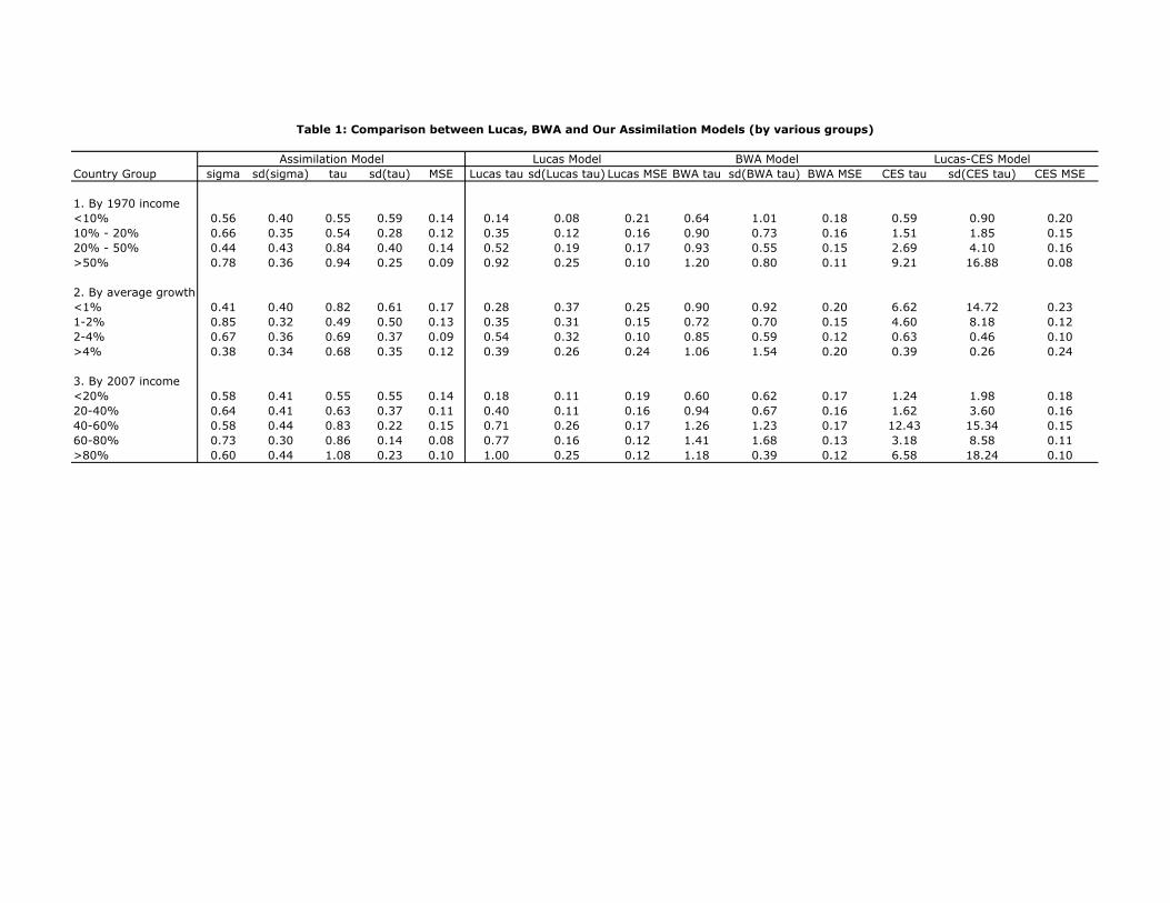
sigma sd(sigma) tau sd(tau) MSE Lucas tau sd(Lucas tau) Lucas MSE BWA tau sd(BWA tau) BWA MSE CES tau sd(CES tau) CES MSE

1. By 1970 income

<10% 0.56 0.40 0.55 0.59 0.14 0.14 0.08 0.21 0.64 1.01 0.18 0.59 0.90 0.20

10% - 20% 0.66 0.35 0.54 0.28 0.12 0.35 0.12 0.16 0.90 0.73 0.16 1.51 1.85 0.15

20% - 50% 0.44 0.43 0.84 0.40 0.14 0.52 0.19 0.17 0.93 0.55 0.15 2.69 4.10 0.16

>50% 0.78 0.36 0.94 0.25 0.09 0.92 0.25 0.10 1.20 0.80 0.11 9.21 16.88 0.08

2. By average growth

<1% 0.41 0.40 0.82 0.61 0.17 0.28 0.37 0.25 0.90 0.92 0.20 6.62 14.72 0.23

1-2% 0.85 0.32 0.49 0.50 0.13 0.35 0.31 0.15 0.72 0.70 0.15 4.60 8.18 0.12

2-4% 0.67 0.36 0.69 0.37 0.09 0.54 0.32 0.10 0.85 0.59 0.12 0.63 0.46 0.10

>4% 0.38 0.34 0.68 0.35 0.12 0.39 0.26 0.24 1.06 1.54 0.20 0.39 0.26 0.24

3. By 2007 income

<20% 0.58 0.41 0.55 0.55 0.14 0.18 0.11 0.19 0.60 0.62 0.17 1.24 1.98 0.18

20-40% 0.64 0.41 0.63 0.37 0.11 0.40 0.11 0.16 0.94 0.67 0.16 1.62 3.60 0.16

40-60% 0.58 0.44 0.83 0.22 0.15 0.71 0.26 0.17 1.26 1.23 0.17 12.43 15.34 0.15

60-80% 0.73 0.30 0.86 0.14 0.08 0.77 0.16 0.12 1.41 1.68 0.13 3.18 8.58 0.11

>80% 0.60 0.44 1.08 0.23 0.10 1.00 0.25 0.12 1.18 0.39 0.12 6.58 18.24 0.10

Country Group

Assimilation Model Lucas Model BWA Model Lucas-CES Model

Table 1: Comparison between Lucas, BWA and Our Assimilation Models (by various groups)

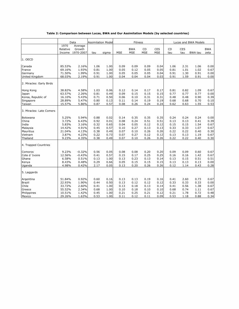
1970

Relative

Income

Average

Growth

1970-2007 tau sigma MSE

BWA

MSE

CD

MSE

CES

MSE

CD

tau

CES

tau BWA tau

BWA

zeta

1. OECD

Canada 85.53% 2.16% 1.06 1.00 0.09 0.09 0.09 0.04 1.06 2.31 1.06 0.00

France 69.16% 1.93% 0.81 1.00 0.05 0.12 0.05 0.05 0.81 1.01 1.02 0.67

Germany 71.50% 1.99% 0.91 1.00 0.05 0.05 0.05 0.04 0.91 1.30 0.91 0.00

United Kingdom 68.03% 2.19% 0.91 1.00 0.04 0.04 0.04 0.03 0.91 1.59 0.91 0.00

2. Miracles: Early Birds

Hong Kong 38.82% 4.58% 1.03 0.06 0.12 0.14 0.17 0.17 0.81 0.82 1.09 0.67

Japan 63.57% 2.26% 0.81 0.49 0.09 0.15 0.15 0.15 0.77 0.77 0.77 0.00

Korea, Republic of 16.10% 5.43% 0.71 0.50 0.06 0.10 0.31 0.31 0.48 0.48 0.90 0.39

Singapore 28.89% 5.47% 0.80 0.13 0.11 0.14 0.19 0.19 0.68 0.68 0.70 0.10

Taiwan 15.57% 5.86% 0.87 0.57 0.08 0.26 0.24 0.24 0.62 0.63 1.55 0.53

3. Miracles: Late Comers

Botswana 5.25% 5.94% 0.88 0.02 0.14 0.35 0.35 0.35 0.24 0.24 0.24 0.00

China 3.72% 6.43% 0.92 0.01 0.08 0.24 0.51 0.51 0.13 0.13 0.41 0.39

India 5.83% 3.16% 0.32 0.65 0.04 0.05 0.12 0.12 0.15 0.15 1.54 0.67

Malaysia 14.42% 4.91% 0.45 0.57 0.10 0.27 0.13 0.13 0.33 0.33 1.07 0.67

Mauritius 21.04% 4.13% 0.38 0.49 0.07 0.10 0.26 0.26 0.22 0.22 0.40 0.30

Vietnam 3.87% 4.23% 0.22 0.73 0.07 0.27 0.12 0.12 0.13 0.13 1.19 0.67

Thailand 9.23% 4.35% 0.38 0.49 0.07 0.10 0.26 0.26 0.22 0.22 0.40 0.30

4. Trapped Countries

Comoros 9.23% -0.32% 0.56 0.05 0.08 0.08 0.20 0.20 0.09 0.09 0.60 0.67

Cote d`Ivoire 12.56% -0.43% 0.41 0.57 0.15 0.17 0.25 0.25 0.16 0.16 1.42 0.67

Ghana 6.58% 0.51% 0.13 1.00 0.13 0.23 0.13 0.14 0.13 0.15 0.51 0.51

Kenya 8.43% 0.48% 0.29 0.66 0.05 0.15 0.15 0.15 0.13 0.13 0.13 0.00

Uganda 4.98% 0.42% 2.17 0.05 0.13 0.20 0.26 0.26 0.12 1.14 0.43 0.28

5. Laggards

Argentina 51.84% 0.92% 0.60 0.16 0.13 0.13 0.19 0.16 0.41 2.60 0.73 0.67

Brazil 22.93% 1.90% 0.44 0.50 0.13 0.12 0.12 0.12 0.33 0.33 0.33 0.00

Chile 33.72% 2.60% 0.41 1.00 0.13 0.18 0.13 0.14 0.41 0.56 1.38 0.67

Greece 55.52% 2.34% 0.68 1.00 0.10 0.18 0.10 0.10 0.68 0.74 1.11 0.67Philippines 10.51% 1.42% 0.45 1.00 0.21 0.25 0.21 0.12 0.21 1.78 0.72 0.48

Mexico 29.26% 1.63% 0.53 1.00 0.11 0.12 0.11 0.09 0.53 1.18 0.88 0.34

Lucas and BWA ModelsData

Table 2: Comparison between Lucas, BWA and Our Assimilation Models (by selected countries)

Assimilation Model Fitness

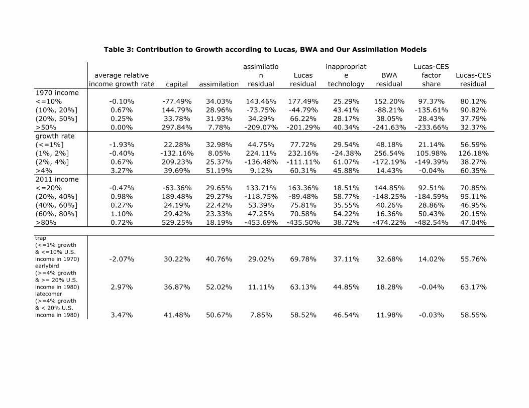
average relative

income growth rate capital assimilation

assimilatio

n

residual

Lucas

residual

inappropriat

e

technology

BWA

residual

Lucas-CES

factor

share

Lucas-CES

residual

1970 income

<=10% -0.10% -77.49% 34.03% 143.46% 177.49% 25.29% 152.20% 97.37% 80.12%

(10%, 20%] 0.67% 144.79% 28.96% -73.75% -44.79% 43.41% -88.21% -135.61% 90.82%

(20%, 50%] 0.25% 33.78% 31.93% 34.29% 66.22% 28.17% 38.05% 28.43% 37.79%

>50% 0.00% 297.84% 7.78% -209.07% -201.29% 40.34% -241.63% -233.66% 32.37%

growth rate

(<=1%] -1.93% 22.28% 32.98% 44.75% 77.72% 29.54% 48.18% 21.14% 56.59%

(1%, 2%] -0.40% -132.16% 8.05% 224.11% 232.16% -24.38% 256.54% 105.98% 126.18%

(2%, 4%] 0.67% 209.23% 25.37% -136.48% -111.11% 61.07% -172.19% -149.39% 38.27%

>4% 3.27% 39.69% 51.19% 9.12% 60.31% 45.88% 14.43% -0.04% 60.35%

2011 income

<=20% -0.47% -63.36% 29.65% 133.71% 163.36% 18.51% 144.85% 92.51% 70.85%

(20%, 40%] 0.98% 189.48% 29.27% -118.75% -89.48% 58.77% -148.25% -184.59% 95.11%

(40%, 60%] 0.27% 24.19% 22.42% 53.39% 75.81% 35.55% 40.26% 28.86% 46.95%

(60%, 80%] 1.10% 29.42% 23.33% 47.25% 70.58% 54.22% 16.36% 50.43% 20.15%

>80% 0.72% 529.25% 18.19% -453.69% -435.50% 38.72% -474.22% -482.54% 47.04%

trap

(<=1% growth

& <=10% U.S.

income in 1970) -2.07% 30.22% 40.76% 29.02% 69.78% 37.11% 32.68% 14.02% 55.76%earlybird

(>=4% growth

& >= 20% U.S.

income in 1980) 2.97% 36.87% 52.02% 11.11% 63.13% 44.85% 18.28% -0.04% 63.17%latecomer

(>=4% growth

& < 20% U.S.

income in 1980) 3.47% 41.48% 50.67% 7.85% 58.52% 46.54% 11.98% -0.03% 58.55%

Table 3: Contribution to Growth according to Lucas, BWA and Our Assimilation Models

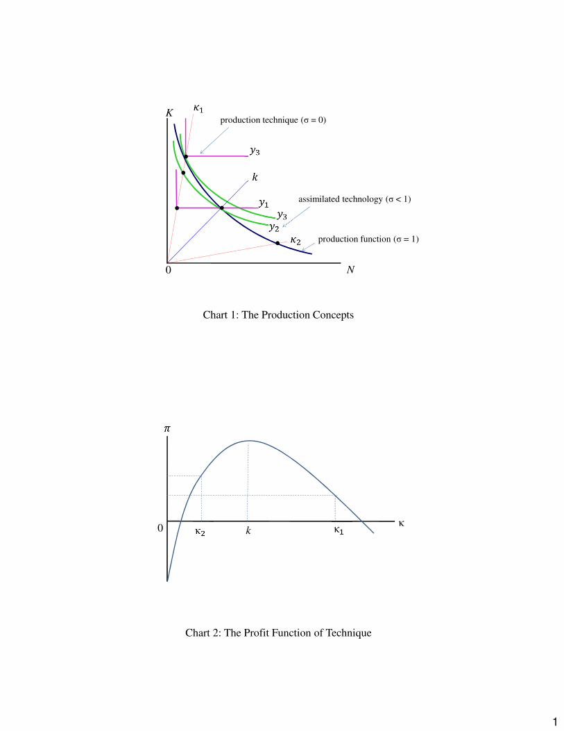
1

production technique (σ = 0)

assimilated technology (σ < 1)

production function (σ = 1)

K

N0

Chart 1: The Production Concepts

•

•

•

•

•

0

Chart 2: The Profit Function of Technique

kκ

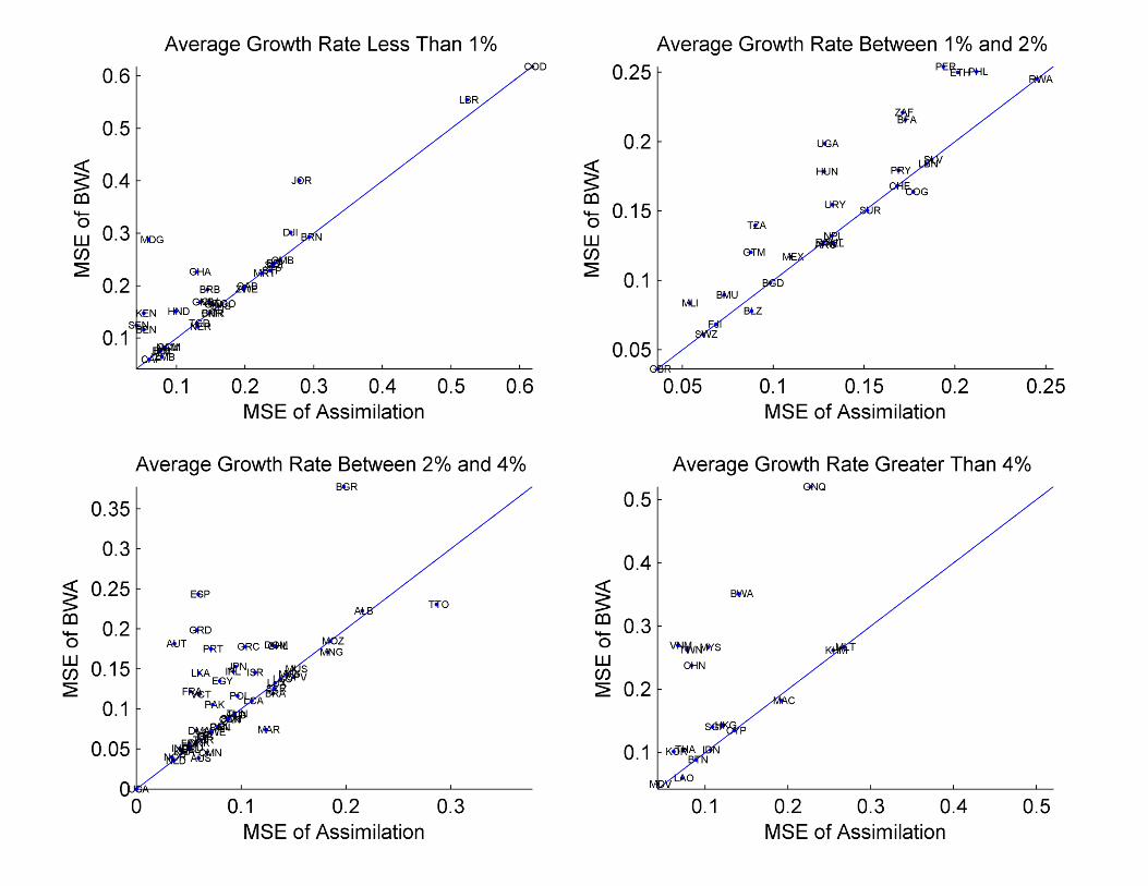
Russell

Typewritten Text

Figure 1a: Model Performance Comparison - Assimilation vs. BWA

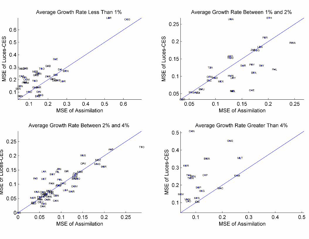
Russell

Typewritten Text

Figure 1b: Model Performance Comparison - Assimilation vs. Lucas-CES

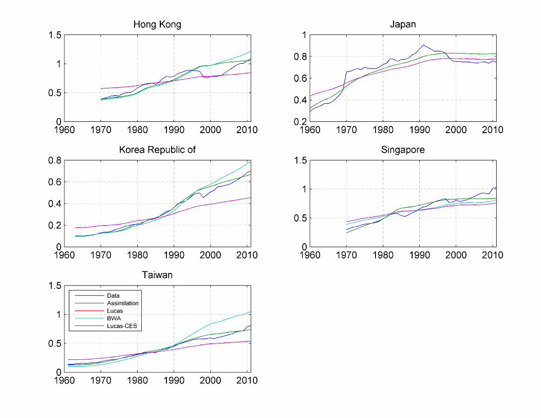
Russell

Typewritten Text

Figure 2: Assimilation Dynamics - Early Birds

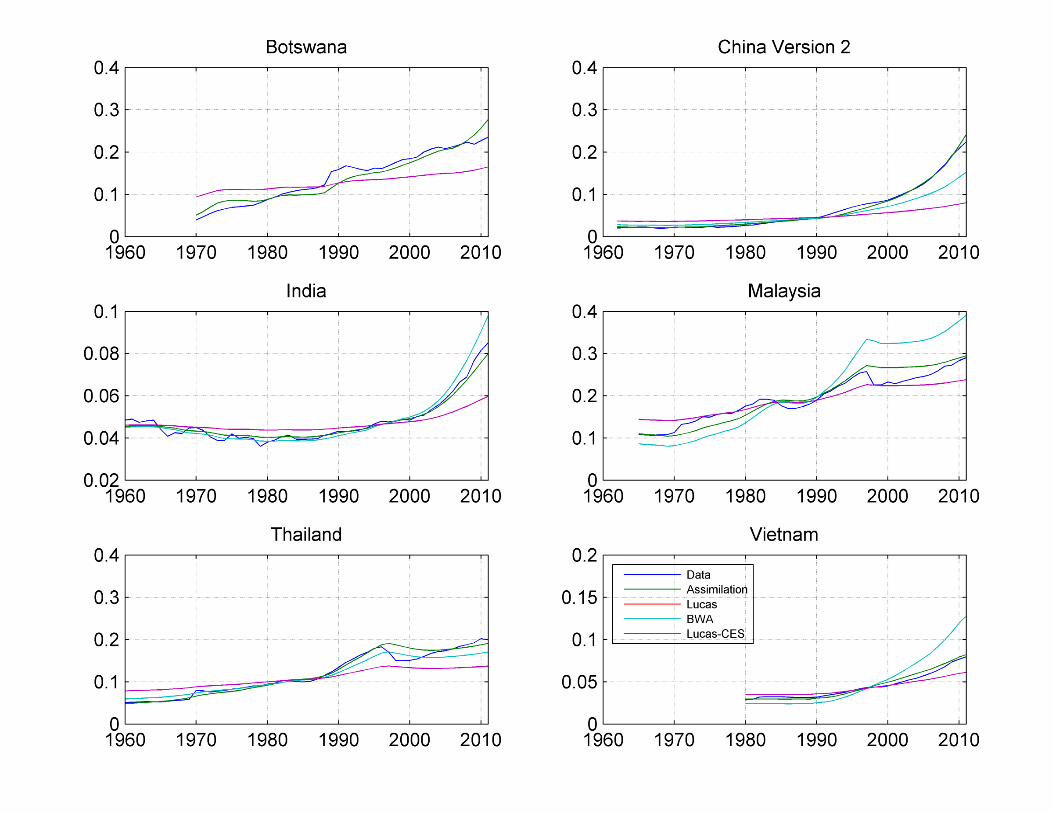
Russell

Typewritten Text

Figure 3: Assimilation Dynamics - Latecomers