Regional Convergence and Aggregate Growth(Preliminary Version)

Stephane Adjemian∗, Jerome Glachant†and Charles Vellutini‡

January, 2000

Abstract

A striking feature of US states convergence is the link betweenthe spatial speed of convergence and the aggregate growth rate: fastaggregate growth induces a reduction in regional inequalities. This pa-per uses a neoclassical growth framework with integrated economies inorder to capture this phenomena. As it has been stressed by Ventura[1997], the interdependence between regional economies through theaccess to common markets generates a link between aggregate evo-lution and spatial convergence dynamics. The paper has two mainsresults. First, we show how deep parameters of the economy deter-mines quantitatively the magnitude of this link. Second, we proposetwo directions for testing the model and we provide some empiricalevidence using US states data on personal income. These results aremixed, only a part of the convergence pattern is well captured by themodel.

1 Introduction

Regional convergence appears to be time varying, and, in most cases, grad-ually slowing down. In the USA, Sherwood-Call [1996] has documented thedivergence in state incomes that took place in the 80’s, after decades ofconvergence. Martin [1997] reports that the speed of convergence among Eu-ropean regions fell from 2% to 1.3%, also in the 80’s. Barro and Sala-I-Martin[1995, chap. 11] have evidenced a significant fall in the speed of convergenceamong Japanese prefectures after 1955. De La Fuente [1998] reports thatconvergence in Spanish regional incomes also shows a marked tendency todecelerate.

∗EPEE, Universite d’Evry-Val-d’Essonne, bld. Francois Mitterrand, 91025 Evry Cedex,France. <adjemian@eco.univ-evry.fr>†EPEE, Universite d’Evry-Val-d’Essonne. <glachant@eco.univ-evry.fr>‡EUREQUA, Universite de Paris I, 106-112, bld de l’Hopital - 75647 Paris Cedex 13,

France. <vellutin@club-internet.fr>

1

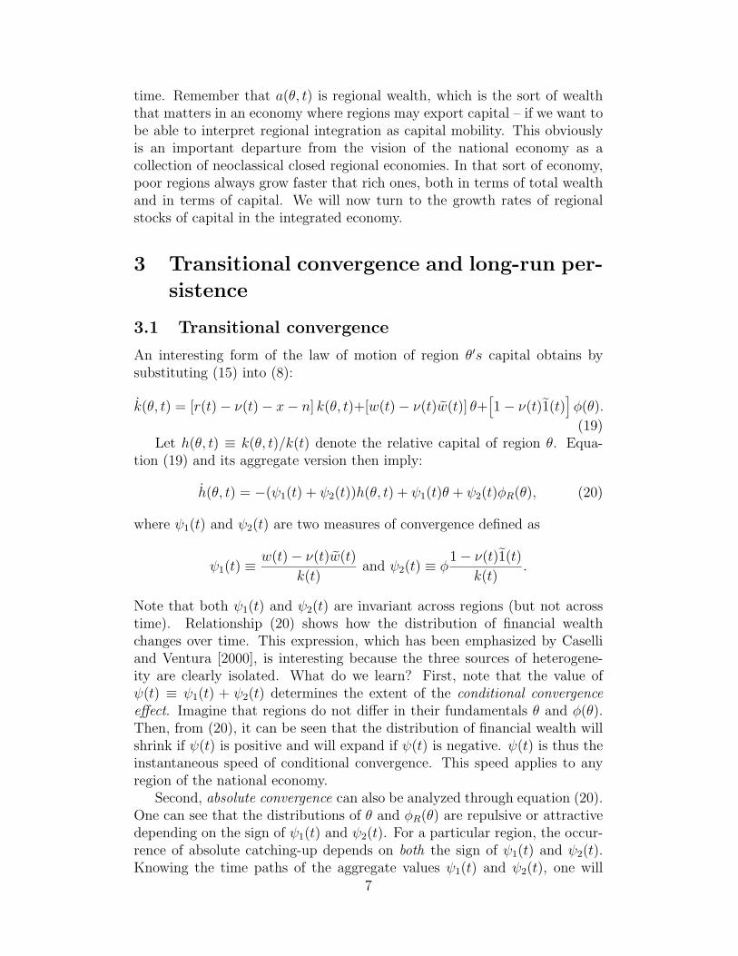
In figure 1, the solid line stands for the speed of convergence among USstates’ relative incomes1. Without performing formal tests, the instability ofthe spatial speed of convergence seems to be a crucial feature of US regionalgrowth dynamics. In the same figure a dashed line represents the annualaverage, over ten years intervals, growth rate of US national income. Itappears that the series are strongly correlated (the correlation is 0.8055),highlighting the link between aggregate growth and regional convergence.

< Insert figure 1. around here >

This paper examines how a neoclassical growth model of integrated economiesmay explain such stylized fact. Using US states income data, we estimate anextended system of growth regression, which make explicit the link betweenspatial convergence and aggregate growth. Our results are mixed, only a partof the convergence pattern is well captured by the model.

We use the neoclassical model that has been constructed by Caselli andVentura [2000] to study distributive dynamics among infinitely lived individ-uals in a particular economy. We follow Bliss [1995] and Ventura [1997], whohave applied the model to study inequality among regions/countries. Ourbasic framework is a general equilibrium growth model, as this is a simpleand natural way to deal with interactions among regional economies. Fac-tor price equalization is achieved without any restrictions and the optimalbehavior of Ramsey savers determines the dynamics of wealth and income.

Bliss [1995] has shown that in this setting, globalization promotes long-run income inequality. More precisely, factor price equalization deters con-vergence so that initial differences in income persist forever. However, Caselliand Ventura [2000] and Ventura [1997] have shown that convergence may ex-ist during the transition of the aggregate economy toward its steady-state. Incontrast with the closed model, conditional convergence is due to the prop-erties of intertemporal demand – not diminishing returns. These articles donot indicate exactly how these theoretical results can be confronted with em-pirical evidence on the distribution of income across regions. There remainsan important gap to bridge between these theoretical criticisms and theirempirical counterparts. The paper provides an empirical strategy for testingthe effect of integration on convergence.

The findings of this paper are as follows. First, the model provides oneexplanation for the deceleration of convergence reported above, as we simul-taneously have a model that can display convergence during the transitionand long-run persistence. The relationship between the dynamics of cross-section inequality and aggregate growth is made explicit by a linearizationaround the steady-state. This local characterization makes it possible torelate the magnitude of the convergence or divergence effect to the param-eters describing the fundamentals of economies. Second, we develop testing

1These estimates are obtained by estimating a cross-region growth equation (See Barroand Sala-I-Martin [1995]) with regional dummies over moving ten years intervals, on theperiod 1939-1997

2

strategies that are based on the linearized version of the model. A paneldata study, which consists in estimating an “extended” system of growthrate regressions with fixed effect, can potentially discriminate between themodel of the integrated economy presented below and the traditional modelof autarchic economies. Third, we provide empirical evidence using US statesdata on personal income.

The paper is organized as follows. In the second section, we present thebasic setup borrowed from Caselli and Ventura [2000]. The third sectioncontains the core theoretical results of the article. We detail how the dis-tribution dynamics displays both persistence and conditional convergence ordivergence. Section 4 provides a testing strategy and section 5 the estimationresults. We conclude in the last section

2 Basic framework

2.1 Structure of the economy and technology

2.1.1 Static structure

The aggregate economy consists of a collection of regions indexed by theirrelative labor productivity θ ∈]0, θmax]. In per capita terms, the regionaltechnology is given by:

Y (θ) = f [K(θ), Aθ] + Aφ(θ), (1)

where Y (θ) and K(θ) are respectively the domestic product and the domesticcapital stock of region θ, both in per capita terms. A is the aggregate levelof technological efficiency growing at a constant exogenous rate x and f(·)is a neoclassical production function. φ(θ) is a constant parameter, eitherpositive or negative. φ(θ) < 0 means that a subsistence consumption levelabsorbs part of the output. φ(θ) > 0 can be viewed as a fixed rent increasingoutput, for example some production using only specific factors that regionθ alone possesses.

(θ, φ(θ)) is therefore time-invariant and characterizes the technology usedby region θ. To do away with certain technical difficulties, these quantitiesare specified in intensive terms2. We will use lower-case letters to denoteintensive variables: for all per capita variable Z, z = Z/A.

We therefore have three sources of region heterogeneity: capital stockK(θ), labor productivity θ and the parameter φ(θ). We note q(B) the numberof regions with productivity index θ ∈ B. We normalize θ and the size ofthe aggregate economy so that

∫ θmax0 θq(dθ) =

∫ θmax0 q(dθ) = 1. It is assumed

that the population grows at the exogenous rate n and that the population is

2Ben-David [1998] studies the case in which the subsistence level is not indexed ontechnological change. Interestingly, endogenous formation of clubs may arise.

3

identical in any region3. In this context, A is the average labor productivityin the aggregate economy. We note the average value of the φ(θ)′s as φ ≡∫ θmax

0 φ(θ)q(dθ). Under the condition φ 6= 0, we then define the relative valueof φ(θ) as φR(θ) ≡ φ(θ)/φ.

Before we proceed to integrate the economy, let us first recall that inregional autarchy the quantity f [K(θ), θA] + φ(θ)A is both the GNP andthe GDP of region θ. From this point on, we assume that the economy isintegrated through perfect capital mobility. It is now necessary to distinguishbetween the capital owned by a given region, noted k(θ), and the capitalused by that region, noted k(θ). The quantity k(θ)− k(θ) is accordingly theportion of region θ′s capital installed abroad. The gross rental rate of capitalis noted r + δ, with δ > 0 the capital depreciation rate. With an integratedmarket for capital, r + δ must be identical across regions. In each country,competitive firms equate the gross marginal productivity of capital to thegross rental rate:

f1

[k(θ), θ

]= r + δ. (2)

With f(·) homogeneous of degree one, equation (2) implies k(θ) = θk(1).With our normalization, national and average quantities are equal:

k ≡∫k(θ)q(dθ) =

∫k(θ)q(dθ) ≡ k. (3)

k is the national capital stock, the average installed capital stock as well asthe capital stock installed in the average region. The capital stock installedin θ therefore satisfies:

k(θ) = θk = θk. (4)

We can now write the GNP of region θ as

y(θ) = θf(k) + φ(θ) + (r + δ)(k(θ)− θk), (5)

where f(k) ≡ f(k, 1).The real wage in country θ satisfies:

w(θ) = θf2(k, θ) = θf2(k, 1) = θw. (6)

Hence, in the integrated economy, factor prices (r(t) and w(t)) are identicalin any region, for all t.

The world output is:

y =∫ (

f[k(θ), θ

]+ φ(θ)

)q(dθ) = f(k) + φ.

As is well known, the complete integration of the national economy im-plies instantaneous conditional convergence (at the precise moment when

3This does not imply any loss of generality, while it simplifies the notation. Our resultsobtain with any distribution of the total population.

4

the world economy is integrated) of the gross domestic product (adjusted forφ(θ)):

y(θ)− φ(θ) = θ(y − φ), for all θ. (7)

In contrast, there is no instantaneous convergence effect affecting the GNPy(θ). This quantity depends on region θ′s wealth, as is shown in equation (5).

2.1.2 Dynamic structure

Time is continuous. The capital of region θ is driven by:

k(θ) = θw + rk(θ) + φ(θ)− c(θ)− (n+ x)k(θ), k(θ, 0) given, (8)

with c(θ) the consumption level of region θ.We rule out Ponzi games by assuming:

limt→∞

e−R(0,t)e(x+n)tk(θ, t) ≥ 0, (9)

where R(0, t) ≡∫ t

0 r(s)ds.Aggregating these equations over regions yields the law of motion of the

national capital stock:

k = f(k) + φ− (δ + x+ n)k − c, k(0) given. (10)

2.2 Households

The representative household of region θ maximizes:

U(θ) =∫ ∞

0

C1−σ(θ, t)− 1

1− σente−ρtdt, (11)

subject to constraints (8-9) and taking the time paths of prices as given.C(θ, t) is per capita consumption in region θ at time t, σ > 0 the inverse ofthe constant intertemporal elasticity of substitution, and ρ > 0 the utilitydiscount rate. In contrast with autarchy, the assumption that householdsmaximize intertemporal utility – as opposed to the choice of some exogenoussaving rates – is central to the convergence results of the integrated model.This point will become clearer later.

With these preferences, it is possible to interpret φ(θ) as a measure ofintertemporal flexibility: the larger φ(θ), the more flexible is region θ in itsintertemporal allocation of consumption. With a negative φ(θ), region θ willnot be able to substitute consumption through time above a certain level.Conversely, a positive φ(θ) means that there is at any time a constant sourceof output which is by definition completely independent of region θ′s timeallocation problem and therefore raises its ability to substitute consumptionintertemporally.

Note that by simply defining Csg(θ) = C(θ) − φ(θ)ext together withtechnology y(θ) = f [k(θ), θ], it is possible to rewrite the maximization prob-lem above with a standard Stone-Geary intertemporal utility function. This

5

setting is fully equivalent to the one used here, but makes the economicinterpretation of a positive φ(θ) more difficult.

As pointed out by Caselli and Ventura [2000], these preferences thus makeit possible to describe the aggregate economy as a hypothetical representativeregion endowed with exactly average characteristics. Aggregate paths arefound by solving the usual autarchy problem, which leads to:

c = c[σ−1 (f ′(k)− δ − ρ)− x

], (12)

k = f(k) + φ− c− (n+ δ + x)k, k(0) > 0 given. (13)

This system is appended with the transversality condition, that is, inequality(9) taken as an equality. As is well known, we need the following conditionon parameters so that this condition always holds in equilibrium:

ρ > n+ (1− σ)x. (14)

In the rest of the paper we will find convenient to note the discounted flowof any variable x as: x(t) ≡

∫∞t x(τ)e−R(t,τ)e(τ−t)(x+n)dτ .

Because of the homothetic properties of preferences, the consumption ofany region θ can be written as a linear function of its total wealth, for all t4:

c(θ, t) = ν(t)a(θ, t), (15)

wherea(θ, t) = k(θ, t) + θw(t) + φ(θ)1(t), (16)

and

ν(t) =[∫ ∞t

eR(t,τ)(1−σ)/σ−(τ−t)(ρ/σ−n)dτ]−1

. (17)

The key point in (15) is that ν(t), the propensity to consume out oftotal wealth, is the same for any region θ, depending only on the aggregatebehavior of the national economy. This fact implies that the total wealth ofany region grows at a rate given by the aggregate economy alone. A simpleexpression for that growth rate can be found by taking the time derivativeof (16)5 and substituting from (8):

a(θ, t)

a(θ, t)= r(t)− ν(t)− n− x. (18)

This is a crucial feature of the model. In an economy where factor pricesare equated across regions by factor mobility and/or interregional trade, andwhere preferences are homothetic (in total wealth), all regions accumulatetotal wealth at precisely the same rate – regardless of relative levels at any

4Combine the intertemporal budget constraint c(t) = a(t) with the integral version of(12).

5Notice that ˙x = (r − n− x)x− x.

6

time. Remember that a(θ, t) is regional wealth, which is the sort of wealththat matters in an economy where regions may export capital – if we want tobe able to interpret regional integration as capital mobility. This obviouslyis an important departure from the vision of the national economy as acollection of neoclassical closed regional economies. In that sort of economy,poor regions always grow faster that rich ones, both in terms of total wealthand in terms of capital. We will now turn to the growth rates of regionalstocks of capital in the integrated economy.

3 Transitional convergence and long-run per-

sistence

3.1 Transitional convergence

An interesting form of the law of motion of region θ′s capital obtains bysubstituting (15) into (8):

k(θ, t) = [r(t)− ν(t)− x− n] k(θ, t)+[w(t)− ν(t)w(t)] θ+[1− ν(t)1(t)

]φ(θ).

(19)Let h(θ, t) ≡ k(θ, t)/k(t) denote the relative capital of region θ. Equa-

tion (19) and its aggregate version then imply:

h(θ, t) = −(ψ1(t) + ψ2(t))h(θ, t) + ψ1(t)θ + ψ2(t)φR(θ), (20)

where ψ1(t) and ψ2(t) are two measures of convergence defined as

ψ1(t) ≡ w(t)− ν(t)w(t)

k(t)and ψ2(t) ≡ φ

1− ν(t)1(t)

k(t).

Note that both ψ1(t) and ψ2(t) are invariant across regions (but not acrosstime). Relationship (20) shows how the distribution of financial wealthchanges over time. This expression, which has been emphasized by Caselliand Ventura [2000], is interesting because the three sources of heterogene-ity are clearly isolated. What do we learn? First, note that the value ofψ(t) ≡ ψ1(t) + ψ2(t) determines the extent of the conditional convergenceeffect. Imagine that regions do not differ in their fundamentals θ and φ(θ).Then, from (20), it can be seen that the distribution of financial wealth willshrink if ψ(t) is positive and will expand if ψ(t) is negative. ψ(t) is thus theinstantaneous speed of conditional convergence. This speed applies to anyregion of the national economy.

Second, absolute convergence can also be analyzed through equation (20).One can see that the distributions of θ and φR(θ) are repulsive or attractivedepending on the sign of ψ1(t) and ψ2(t). For a particular region, the occur-rence of absolute catching-up depends on both the sign of ψ1(t) and ψ2(t).Knowing the time paths of the aggregate values ψ1(t) and ψ2(t), one will

7

know how regions move toward their long-run position. In subsection 3.3,we study how these coefficients change in the neighborhood of the aggregatesteady-state. The occurrence of local conditional convergence or divergencedepends on the parameters describing the fundamentals of the economies.Caselli and Ventura [2000] have shown that the model with a CES produc-tion function can display transitional divergence or even successive periods ofconvergence and divergence, a phenomenon reminiscent of a Kuznets curve.

In fact, in this economy, a key determinant of transitional convergence isthe elasticity of substitution between factors. Consider (16) and (18): regard-less of the share of financial wealth in its total wealth, any region will find itoptimal to accumulate the latter at the same rate. Think of a high elasticityof substitution. As the aggregate economy accumulates capital, the demandfor labor will tend to be relatively low because the economy will increas-ingly substitute capital for labor. So will be the discounted flow of wages,a component of total wealth (”human” wealth). Finally, one sees that tokeep total wealth on an optimal path, regions poorly endowed with financialwealth will need to accumulate it at a quicker rate than the financially rich.An alternative expression for ψ illustrates this point. From (18):

ψ(t) =k(t)

k(t)− a(t)

a(t). (21)

This relationship shows that if, in aggregate terms, the growth rate ofcapital is higher than that of total wealth, there will be transitional condi-tional convergence.

Another point is worth emphasizing here. The important underlying mech-anism for transitional convergence is the homothetic property of householdpreferences, not diminishing returns to capital like in the autarchic model.In this economy, transitional divergence in capital stocks is plausible eventhough technology is one with diminishing returns.

3.2 Long-run persistence of the cross-section distribu-tion

Integrating (20) yields:

h(θ, t) = λ1(0, t)h(θ, 0) + λ2(0, t)θ + λ3(0, t)φR(θ), (22)

where

λ1(0, t) = exp[−∫ t

0ψ(s)ds], (23)

λ2(0, t) =∫ t

0ψ1(s)λ1(s, t)ds, (24)

λ3(0, t) =∫ t

0ψ2(s)λ1(s, t)ds. (25)

8

This result has been provided by Caselli and Ventura [2000]. What isinteresting in this relationship is that, again, λ1(0, t), λ2(0, t) and λ3(0, t)are independent of θ. This equation therefore provides a very transparentdecomposition of the distribution of financial wealth at any point in time,making explicit the respective contributions of the initial financial wealthdistribution, the distribution of labor productivity and the distribution ofthe φ(θ)′s. Not surprisingly, given the construction of (22), the λ′is sum upto unity, for all (t, t′)6:

λ1(t, t′) + λ2(t, t′) + λ3(t, t′) = 1. (26)

The variable λ1(t, t′) is a measure of cumulated conditional convergence be-tween t and t′, as opposed to ψ(t′), which may be viewed as the instantaneousconditional convergence at instant t′. It can be seen by direct examinationof (22) taken between t and t′ that if λ1(t, t′) is less that unity, then therewill be cumulated conditional convergence over that period of time.

What does (22) tell us on the asymptotic distribution of financial wealth?In the long run the distribution reads:

h(θ,∞) = λ1(0,∞)h(θ, 0) + λ2(0,∞)θ + λ3(0,∞)φR(θ). (27)

There are no particular reasons why λ1(0,∞) should be equal to zero. Ev-idently, the distribution of long-run financial wealth will be also influencedby the other two sources of heterogeneity, respectively in θ and φ(θ). Butthe important fact is that we have a situation of long-run persistence of thefinancial wealth distribution. In other words, there may well be transitionalconvergence – or divergence –, as was shown in section 3.1, but in all casesthese dynamics will come to an halt as the aggregate economy proceeds to-wards a steady-state. This result is in line with the one obtained by Bliss[1995].

Note that long-run persistence of initial distributions applies in exactlythe same way to consumption: just consider (15) and (16). Income distribu-tion dynamics are slightly more complex because the shares of respectivelycapital and labor incomes in total income may vary over time. It is nonethe-less not difficult to show that long-run persistence also applies. Defining theshare of capital income in total income α(t) ≡ r(t)k(t)/y(t) and the shareof labor income as β(t) ≡ w(t)/y(t), an expression for the relative income ofcountry θ, yR(θ, t) ≡ y(θ, t)/y(t), can be found by substitution into (22):

yR(θ, t′) = γ1(t, t′)yR(θ, t) + γ2(t, t′)θ + γ3(t, t′)φR(θ), (28)

where

γ1(t, t′) =α(t′)

α(t)λ1(t, t′), (29)

γ2(t, t′) = β(t′) + α(t′)λ2(t, t′)− α(t′)

α(t)β(t)λ1(t, t′), (30)

γ3(t, t′) = 1− γ1(t, t′)− γ2(t, t′). (31)6One way to do this is to sum (22) over the θ′s.

9

A different way of writing equation (28) is to make explicit the income“target” of region θ:

yR(θ, t′) = γ1(t, t′)yR(θ, t) + (1− γ1(t, t′))y?R(θ, [t, t′]), (32)

where the income target y?R(θ, [t, t′]) is defined as:

y?R(θ, [t, t′]) =γ2(t, t′)

γ2(t, t′) + γ3(t, t′)θ +

γ3(t, t′)

γ2(t, t′) + γ3(t, t′)φR(θ). (33)

On the one hand, these results are reminiscent of the autarchic model,in the sense that the dynamics is still guided by a gap between the currentvalue of the variables (e.g. relative income yR(t)) and some long run “tar-get”. On the other hand, observe that in the integrated economy, this targetis time-varying and, more importantly, can never be attained. The modelcontrasts sharply with the long-run behavior of economies in the autarchicmodel. One key result of that setting is that any regional economy convergesto a unique steady-state level of wealth and income – conditional on struc-tural parameters such the labor productivity and preferences. This processwill eventually iron out initial income differences. Here, on the contrary, theeffects of initial wealth will be felt forever. Each region will reach its own par-ticular steady-state level of financial wealth and income – even if conditionedon structural parameters. Put differently, there are no stationary wealth andincome distributions.

3.3 Characterization around the aggregate steady-state

One way to understand how the distribution of financial wealth changes asthe aggregate economy grows towards its steady-state is to linearize equa-tion (22) around the aggregate steady-state. To do this, we need to study thecoefficients λi(t, t

′), i = 1, 2, 3, or alternatively ψ(t), ψ1(t) and ψ2(t), aroundthe steady-state.

Note that for this purpose it is easiest “to eliminate time” and to workwith aggregate quantities as functions of the capital stock k, not t. A well-known example of this are the policy rules c(k), a(k), w(k),etc. Similarly, wedefine λ1(k, k′) as the value taken by the coefficient λ1 when the aggregateeconomy starting from k moves to k′. In the same fashion, we can defineλi(k, k

′), i = 2, 3, ψi(k), i = 1, 2 and ψ(k). Let k? denote the steady stateaggregate level of capital.

First, these functions satisfy: λ1(k?, k?) = 1, λ2(k?, k?) = λ3(k?, k?) = 0,and ψ1(k?) = ψ2(k?) = ψ(k?) = 0. Second, we define η?i , i = 1, 2, 3 asthe semi-elasticities of the function λi(k, k

?), i = 1, 2, 3 with respect to k,evaluated at k = k?:

η?i ≡ k?(∂λi(k, k

?)

∂k

)k=k?

, i = 1, 2, 3. (34)

10

Taking the first order Taylor expansion of λi(k, k′) near the steady-state

yields:

λi(k, k?) ≈ λi(k

?, k?) + η?i

[k − k?

k?

], i = 1, 2, 3. (35)

Moreover, since the coefficients λi, i = 1, 2, 3 sum up to unity, we have:

η?1 + η?2 + η?3 = 0. (36)

Assuming that the initial aggregate capital stock k(0) is not too far offk?, and neglecting second order terms, the long-run distribution of relativefinancial wealth is given by:

h(θ,∞) =

[1− η?1

(k?

k(0)− 1

)]h(θ, 0)−η?2

(k?

k(0)− 1

)θ−η?3

(k?

k(0)− 1

)φR(θ).

(37)This equation can be interpreted as follows. Imagine that the aggregate

economy is below its steady-state (k(0) < k?), so that the economy experi-ences an episode of growth at a cumulated rate k?/k(0)−1. Then, the initialdistribution of the h(θ, 0)′s shrinks or expands – depending on the sign ofη?1. If η?1 > 0, aggregate growth implies a phenomenon of conditional con-vergence. Relative productivity level θ has a positive influence on long-runrelative wealth as long as η?2 < 0. The influence of φ(θ) depends on the signof η?3.

In Appendices B and C, we show that the coefficients η?i , i = 1, 2, 3 canbe expressed as functions of the deep parameters of the model:

η?1 = 1− k?

c?[ρ+ σ(x+ µ)− (n+ x)] , (38)

η?2 =k?

c?σµ− w?

c?, (39)

η?3 = − φc?, (40)

where µ > 0 is the speed of convergence of the aggregate economy toward itssteady-state (see Appendix A).

Moreover, we show in the appendices that:

ψ′(k?) = −µη?1

k?, ψ′1(k?) = µ

η?2k?, ψ′2(k?) = µ

η?3k?. (41)

These equations provide a full characterization of the cross-section dynamicsaround the steady-state. In particular, we see how the parameters describingpreferences and technology influence the distribution of wealth across regions.

One of the most interesting results is the negative relationship betweenµ, the aggregate speed of convergence, and η?1, a measure of the conditionalconvergence effect. We see that a slow adjustment of the world economy

11

translates into a low long-run persistence of the distribution of financialwealth. Ventura [1997] already identified this property of the model, butwithout quantifying it. Knowing that ε, the elasticity of substitution of theproduction function, and σ, the inverse of the intertemporal elasticity of sub-stitution, both impact negatively on µ, one can conclude that the size of thelong-run persistence effect decreases with these parameters. By contrast, thissize increases with φ, the average level of the φ(θ)’s.

From (38), one can see that the most realistic configuration of the pa-rameters leads to a conditional convergence effect7. A conditional divergenceeffect would take place only for high values of µ and σ. Also, the influence ofφ(θ) on the long-run wealth is always positive. The influence of the relativeproductivity level θ depends on the sign of η?2. Some kind of substitutioneffect between financial and human wealths cannot be ruled out. Indeed,η?2 > 0 would mean that regions poorly endowed in terms of θ make up fortheir low labor productivity by accumulating financial wealth at a faster rate.It could be the case for high values of σ and µ8.

Starting from (28), we can use the same analysis to study the behavior ofthe distribution of relative gross income yR(θ). Appendix D focuses on thedetermination of the semi-elasticities ωi, i = 1, 2, 3 of the coefficients γi. Theresults obtained for the distribution of relative wealth h(θ) must be amendedso as to take into account the fact that respective factor shares in total incomemay be variable around the aggregate steady state. This exercise clarifiesthe influence of a high elasticity of substitution on the income distribution.First, a high value of ε tends to depress the growth of wages and hence favorsconditional convergence of relative wealth, as was noted above. But we havea second effect here. A high value of ε also implies a strong decrease of theshare of wage in total income when the aggregate economy converges towardits steady-state. This second effect weakens conditional convergence.

4 Strategies for empirical testing

In this section, we give directions along which the above results could betested. A key preoccupation is to focus on the discriminating predictions ofthe model – particularly, on what distinguishes the integrated national econ-omy from a collection of autarchic regions. A prediction of the model whichclearly possesses this discriminating property is the long-run persistence ofinitial conditions, in other words, that convergence, when it exists, will neverbe complete. To simplify our exposition in this section, we assume thatθ is the only source of heterogeneity in the fundamentals. More precisely:φ(θ) = 0 for all θ.

7It is important to remember that ρ+ σx is the net rate of interest.8Remember that the η?i relate to one another by (36). Consequently, conditional di-

vergence implies some substitution effect.

12

4.1 Integrated economy vs autarchic economies

A natural route to explore the difference between autarchic and integratedeconomies is to express the distribution of relative incomes as a function ofpast relative incomes and relative fundamentals. In the integrated economy,relationship (32) is available. By contrast, such expression does not existin the autarchic case as the dynamics of aggregate income depends on thedistribution of capital across regions.

A way to solve this difficulty is to linearize the autarchic dynamics aroundthe steady state, as the distribution of capital among regions is uniquelydetermined near the steady state. For any country θ, we have:

y(θ, t′)− y?(θ) = e−µ(t′−t) (y(θ, t)− y?(θ)) , (42)

with µ the speed of convergence of a region toward its steady-state andy?(θ) = θy? the steady-state income of country θ. Note that we used the samesymbol µ for the speed of convergence because such speed is exactly equalto the µ characterizing the aggregate dynamics of the integrated economy.

¿From this, we obtain:

yR(θ, t′) = e−µ(t′−t)yR(θ, t) +(1− e−µ(t′−t)

)θ. (43)

The integrated-economy analogue to this expression, with φ(θ) = 0,comes directly from (32):

yR(θ, t′) = γ1(t, t′)yR(θ, t) + (1− γ1(t, t′))θ. (44)

The comparison (43) and (44) is straightforward. The term e−µ(t′−t)

will tend to zero as t′ grows, whereas its integrated-economy counterpart,the quantity γ1(t, t′), will not. Initial conditions have a persistent effectin the integrated economy. This persistence phenomenon does not exist inthe autarchic economy and convergence will always translate into completecatching-up.

Another way of comparing the respective predictions of the two models isto look at growth rates. To do this, we now have to use the linearized expres-sion of γ1(t, t′) (see Appendix D). We therefore assume that the aggregateeconomy is not too far from a steady state. Let us define :

gR(θ, t, t′) ≡ yR(θ, t′)− yR(θ, t)

yR(θ, t)

as the growth rate of relative income. From (43), an approximate expressionfor this growth rate in the autarchic model is:

gR(θ, t, t′) =(1− e−µ(t′−t)

) [ θ

yR(θ, t)− 1

]. (45)

13

In the integrated economy, one can use the fact that9 1 − γ1(t, t′) ≈ω?1(y(t′)y(t)− 1

), together with (44), results into:

gR(θ, t, t′) = ω?1

(y(t′)

y(t)− 1

)[θ

yR(θ, t)− 1

]. (46)

The comparison between (45) and (46) is again transparent. The behaviorof an integrated economy differs from its autarchic counterpart in one keyaspect: the intensity of convergence effect depends on the aggregate dynamics.As the aggregate economy proceeds toward its steady state, the convergenceeffect dies out.

4.2 A system of modified growth rate regressions

Let us assume that t′ − t = 1 so as to use yearly data and let gR(θ, t) bethe growth rate of relative income between t− 1 and t. From this point on,y will no longer be the intensive level of income per head but will stand forthe level of actual (“extensive”) income per head. The two equations (45)and (46) lead to the following reduced form of the relative income dynamics:

gR(θ, t) = a1+a2y(t)

y(t− 1)+a3(θ)

y(t)

y(θ, t− 1)+a4(θ)

1

yR(θ, t− 1)+u(θ, t). (47)

In each underlying model, the coefficients a1, a2(θ), a3(θ) and a4 are relatedto structural parameters in the following way:

Autarchic economy Integrated economya1 = −(1− e−µ) a1 = ω∗1a2 = 0 a2 = ω∗1a3(θ) = 0 a3(θ) = θω∗1e

−x

a4(θ) = θ(1− e−µ) a4(θ) = −θω∗1

u(θ, t) is an error term10. We allow for some spatial heteroskedasticity.In addition to (47), one can estimate the following structural form:

gR(θ, t) =

(b1 + b2

y(t)

y(t− 1)

)[θ

yR(θ, t− 1)− 1

]+ u(θ, t). (48)

with the following restrictions on parameters:

9Alternatively, it is possible to use the log specification 1− γ1(t, t′) ≈ ω?1 log(y(t′)y(t)

).

10We prefer not to refer to “shocks”, as the introduction of uncertainty at the agent levelwould raise complex theoretical issues related to the desire for some insurance againstidiosyncratic shocs. The term u(θ, t) should be viewed as the sum of whatever is notexplained by the model in the actual trajectories of the variables. It may account forexample for variations known to the agents over their horizon of prevision, which are notmodeled and are unobservable to the econometrician (see for example Altug and Labadie[1994, chap. 7]).

14

Autarchic economy Integrated economyb1 = 1− e−µ b1 = −ω∗1b2 = 0 b2 = ω∗1e

−x

Note that structural parameters in both regimes are exactly identified. Theseequations may be complemented with the dynamics of the aggregate economywhich is identical in the two models:

g(t) =(1− e−µ

) [ ex(t−1)y∗

yR(θ, t− 1)− 1

].

4.3 σ-convergence

Another approach to testing the model relies on studying the changes overtime of the cross-section variance of relative incomes. Since we will study anunivariate time series, panel techniques for controlling possible heterogeneityin underlying parameters will not be available any longer. Taking into ac-count heterogeneity in this setting is in theory still possible, but analyticallyoverly complex. What we will analyze in this subsection is therefore absoluteconvergence, as opposed to conditional convergence. Most authors study-ing convergence in regional data sets have plausibly assumed homogeneity instructural parameters (see for example Barro and Sala-I-Martin [1995, chap.11]). Formally, applying the variance operator to both sides of equation (44)and assuming that all regions have an identical level of labor productivityθ = 1, we have the following law of motion for the cross-region variance ofrelatives incomes:

σ2(t) = σ2u + γ2

1(t− 1, t)σ2(t− 1) (49)

where σ2(t) = V (yr(θ, t)). We used the fact that the error term u(θ, t)appended to (48) is not correlated with yR(θ, t − 1) and assumed that thevariance of u(θ, t), σ2

u, is time-invariant.The autarchic equivalent of this expression is:11

σ2(t) = σ2u + e−2µσ2(t− 1) (50)

There is, again, a crucial difference between the two equations. In theautarchic model, the multiplicative coefficient e−2µ is time-invariant. Its coun-terpart in the integrated economy, γ2

1(t−1, t), will grow monotonically and isasymptotically equal to unity. Using the fact that γ1 is not far from a steadystate, one gets the approximation:

γ21(t− 1, t) ' 2γ1(t− 1, t)− 1 ' 1− 2ω∗1

(y(t)

y(t− 1)− 1

). (51)

11See for example Barro and Sala-I-Martin [1995], page 384.

15

By substituting (51) into (50), by introducing the exogenous technical progressx and adding an error term similar to u(θ, t), we finally get the regression tobe tested:

σ2(t) = σ2u + (1 + 2ω∗1)σ2(t− 1)− 2ω∗1e

−x y(t)

y(t− 1)σ2(t− 1) + ε(t). (52)

5 Some evidence from the US states

The US states data seem to be an most ideal starting point for several reasons.First, as we noted above, there is substantial evidence of the convergence instate incomes slowing down. Second, data on per capital personal incomehave been compiled by the Bureau of Economic Analysis (BEA) every yearfrom 1929. These are the longest existing series used in the literature onconvergence: 69 years (1929-1997), for the 48 contiguous states. Third, asKim [1997] reports, factors and goods are highly mobile across the US states.The assumption of perfect integration may be plausible in this economy.

The data has been obtained from the BEA’s web page. Personal incomeis provided in nominal terms and it is not possible to deflate the data sincestate-specific deflators are not available. Consequently, relative income percapita are based on nominal levels while the federal consumer price indexhas been used to deflate aggregate nominal income per capita.

We follow the strategy described in the previous section. First, we usepanel data techniques to estimate a system of modified growth rates regres-sions. Second, we study σ−convergence.

5.1 Growth regressions

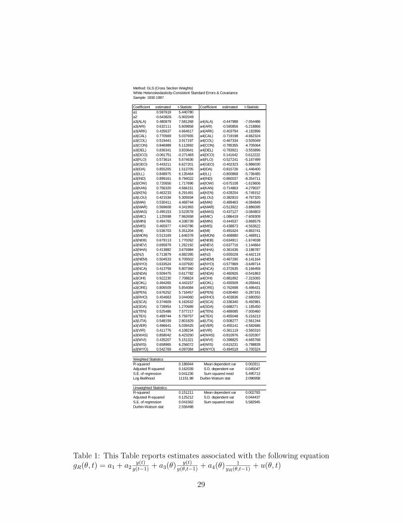
We begin by an estimation of the reduced form (47) using weighted least-squares with White’s correction to account for both spatial and temporalheteroskedasticities. The detailed results are shown in Tables (1 and 2).Most of the estimated coefficients differ significantly from zero. Moreover,the signs of these coefficients are consistent with the model of integration inwhich ω∗1 > 0. Several tests are derived from this estimation:

• We test the restrictions on the parameters implied by the autarchicmodel. The null hypothesis is H0 : a1 = a3(θ) = 0, ∀θ and the asso-ciated Wald statistics is 803,31 which indicates a very strong rejectionof the autarchic model.

• We test the restrictions on the parameters imposed by the integratedmodel. The null hypothesis is H0 : a1/a4 = a2(θ)/a3(θ) = 0, ∀θ andleads to the structural form (48). The Wald statistics is 78.09 with anassociated P-value of 0.0045. This means that the null hypothesis isalso rejected. However, this rejection is not so strong as that of theautarchic model. Moreover, the result of this test is very sensitive to

16

the method of estimation. For instance, without White’s correctionagainst temporal heteroskedasticity, the Wald statistics is 66.93 with aP-value of 0.045.

Second, we estimate the structural form (48) by weighted iterative least-squares. The estimated coefficients are shown in Table (2). Note that thetable in the appendix provides estimates for both the coefficients b1, b2 andthe structural parameters ω∗1 and x. The estimated values of b1 and b2 confirmthat integration matters in the sense that the speed of convergence betweenregions appear to depend on aggregate dynamics. The structural parameterω∗1 is 0.62 with a standard error of 0.053. This means that aggregate growthleads to a reduction of disparities between regions. However, the estimatedvalue of the long-run growth rate x is disappointing. The counterfactualnegative sign of this coefficient implies that a conditional convergence effect ispossible when per capita aggregate income actually falls. An interpretation ofthis is that part of the convergence behavior arises independently of aggregatedynamics.

On balance, these results suggest that the convergence patterns of the USStates may be best represented by a model lying in between the integratedand the autarchic models.

5.2 σ-convergence

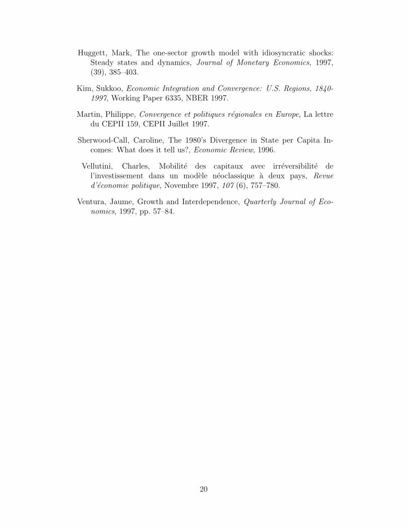
Before we proceed to estimate the model expressed in terms of variances,equation (52), we need to take care of a problem in the data. When it comesto computing cross-section variances, the respective weights of regions mat-ter. It would be misleading to count each region as one observation in thetotal population. To make this point clearer, consider the following thoughtexperiment: split California into two states, each with half of California’spopulation and income. The weight of the Californian growth behavior inthe cross-section variance of relative incomes would suddenly be twice whatit was before – while the economy has not changed a bit. Nor would a simpleweighing by populations result in an accurate calculation of variances, be-cause of the quadratic nature of variance. Appendix E details the procedurewe propose to handle population weights. Given that the variance is basi-cally a sum of squares, the trick is to weigh each state’s relative income withthe square root of its population. Figure 2 gives the variances adjusted forpopulation over time.

< Insert figure 2. around here >

An eye examination of the graph does suggest some tendency for thecross-section variance to stabilize at a strictly positive value. But, withoutany further qualification, this is perfectly compatible with autarchic equation(50). If σ2

u, the variance of the stochastic innovations of relative incomes, is

17

significantly above zero, the autarchic model will display this sort of behav-ior12.

As can be seen from the results of the estimation of (52) in Table1, thedata on US states provide some indication that integration matters. Just likein the β-convergence analysis, the model applied to σ-convergence succeedsin reproducing the data quite well. In particular, the coefficient on Y (t)

Y (t−1)σ2t−1

is statistically significant. Ljung-Box tests performed on the first three lagsdo not reject the null hypothesis of no autocorrelation up to the specifiedlags. The same tests performed on the residuals of equation (51) decisivelyreject the same null hypotheses.

On the other hand, the values of the estimated structural parameters givemore ambiguous information. These values are as follows (standard errorsare shown between brackets): ω∗1 = 0.379 [0.0721] and x = −0.0415 [0.027].While ω∗1 = 0.379 is plausible, the value x = −0.0415, like in our analysis ofβ-convergence, suggests that the convergence behavior of the US States maybe best represented by some sort of cross of the two models.

Table 1: estimation of (52)

Variable Coefficient Std. Error t-Statistic p-ValueIntercept 0.000223 0.000541 0.412670 0.6812

σ2t−1 1.758222 0.144274 12.18669 0.0000

y(t)y(t−1)

σ2t−1 -0.790381 0.145032 -5.449707 0.0000

R-squared: 0.990571 Akaike info criterion: -7.953222Adjusted R-squared: 0.990276 Schwarz criterion: -7.854505

Lag Q′LB statistic p-Value1 0.3398 0.5602 1.6840 0.4313 4.0986 0.251

6 Conclusion

This model provides a theoretical explanation for the deceleration of con-vergence among integrated, i.e. regional economies. When interactions aretaken into account in a Ramsey model of economic growth, a link betweenaggregate growth and regional speed of convergence appears. Our charac-terization makes it possible to confront the model with empirical evidence.The results using US states data are mixed. On the one hand, integrationappears to matter: there are indications that aggregate dynamics contributeto shaping the pattern of convergence among US states. On the other, partof conditional convergence seems not to be connected with the aggregateeconomy.

This analysis highlights the importance of interactions among economiesfor understanding patterns of convergence. We have shown that, in the

12The steady state value for σ2t given by equation (50) is σ2

∞ = σ2u/(1− e−2µ).

18

long run, the influence of integration may run contrary to the traditionalnotion of “equalizing exchange”. Again, it is important to remember thatin this intertemporal utility setting and without any sort of externality, thecounterpart of the long-run persistence result is an improvement of dynamicutility for all regions.

Two promising directions for further research on integration and growthcan be thought of. First, our empirical results suggest that less than per-fect integration should be analyzed, for example through the introduction ofnon-tradables, adjustment costs or investment irreversibility, as in Vellutini[1997]. In the same direction, liquidity constraints as introduced by Huggett[1997] may potentially affect the persistence result. These extensions couldobviously bring additional realism to the model, especially if it is applied tothe world economy. Second, the result of long-run GNP persistence couldalso be modified by mechanisms of technology diffusion. This is clearly avery important extension of the model, as shown by the recent literature onthe subject, for example Basu and Weil [1996] who explore the idea of grad-ual technology diffusion through a mechanisms of “appropriate technology”,or Eeckhout and Jovanovic [1998] who show how non-trivial external effectsgive rise to inequality in productivity.

References

Altug, Sumru and Pamela Labadie, Dynamic Choice and Asset Markets,Academic Press, San Diego, 1994.

Barro, Robert and Xavier Sala-I-Martin, Economic Growth, McGraw Hill,New York, 1995.

Basu, Susanto and David Weil, Appropriate Technology and Growth, Work-ing Paper 5865, NBER December 1996.

Ben-David, Dan, Convergence clubs and subsistence economies, Journal ofDevelopment Economics, 1998, (55), 155–171.

Bliss, Christopher, Capital Mobility, Convergence Clubs and Long-Run Eco-nomic Growth, Technical Report 1995. Paper presented at the 10thEconomic Association Congress.

Caselli, Francesco and Jaume Ventura, A representative Consumer Theoryof Distribution, American Economic Review, 2000. Forthcoming.

Eeckhout, Jan and Boyan Jovanovic, Inequality, Working Paper, Univ. Pom-peu Fabra October 1998.

Fuente, Angel De La, What kind of regional convergence?, Mimeo, IAE, U.Autonoma de Barcelona 1998.

19

Huggett, Mark, The one-sector growth model with idiosyncratic shocks:Steady states and dynamics, Journal of Monetary Economics, 1997,(39), 385–403.

Kim, Sukkoo, Economic Integration and Convergence: U.S. Regions, 1840-1997, Working Paper 6335, NBER 1997.

Martin, Philippe, Convergence et politiques regionales en Europe, La lettredu CEPII 159, CEPII Juillet 1997.

Sherwood-Call, Caroline, The 1980’s Divergence in State per Capita In-comes: What does it tell us?, Economic Review, 1996.

Vellutini, Charles, Mobilite des capitaux avec irreversibilite del’investissement dans un modele neoclassique a deux pays, Revued’economie politique, Novembre 1997, 107 (6), 757–780.

Ventura, Jaume, Growth and Interdependence, Quarterly Journal of Eco-nomics, 1997, pp. 57–84.

20

Technical appendices

A The aggregate economy around its steady-

state

Around the steady-state (c?, k?), the aggregate economy dynamics is charac-terized by the Jacobian matrix:

J =

[0 c?σ−1f ′′(k?)−1 f ′(k?)− (δ + n+ x)

]. (53)

The characteristic polynomial associated to J is:

P (µ) = µ2 − (ρ+ σx− (n+ x))µ+ c?σ−1f ′′(k?). (54)

It is well known that P (µ) has two roots of opposite signs µ1 > 0 and µ2 < 0.Moreover, we know that µ1 + µ2 = Tr(J) = ρ + σx − (n + x). µ = |µ2| > 0is the speed of convergence of the world economy toward its steady-state. Asµ1 × µ2 = Det(J) = c?σ−1f ′′(k?), we obtain:

µ(µ+ ρ+ σx− (n+ x)) = −c?σ−1f ′′(k?). (55)

µ can be expressed as a function of the parameters of preferences andtechnology. Define ε and α as representing respectively the elasticity of sub-stitution between factors of the technology and the share of capital incomein total income13:

ε ≡ −f′(k)(f(k) + φ− kf ′(k))

k(f(k) + φ)f ′′(k), α ≡ kf ′(k)

f(k) + φ. (56)

Let r? = ρ+ σx be the (net) interest rate in he steady-state. The aggregatespeed of adjustment is then given by:

µ =1

2

−(r? − (n+ x)) +

√(r? − (n+ x))2 +

4

εσ(r? + δ)(1− α)

c?

k?

. (57)

Moreover, with our definitions, the ratio c?/k? satisfies:

c?

k?=r? + δ

α− (δ + n+ x).

It is useful to study the local properties of the policy rule c(k) associated tothe competitive aggregate dynamics. We eliminate time in the differentialsystem (12,13) so that:

c′(k) =σ−1(f ′(k)− δ − ρ)c(k)− xc(k)

f(k) + φ− c(k)− (δ + x+ n)k. (58)

13Including φ in these expressions facilitates the algebrical manipulations below.21

Since 0/0 is indeterminate, (58) is uninformative on the value of c′(k?).However, by applying L’Hopital’s rule, it is easy to show that c′(k?) solvesP (µ) = 0. Consequently, there are two candidates for c′(k?): the two eigen-values µ1 and µ2, corresponding respectively to the stable and unstable armsof the phase diagram. It is easy to see that the stable arm has a positiveslope in the (k, c) plan so that:

c′(k?) = µ1 = µ+ ρ+ σx− (n+ x), (59)

is the solution of interest.

B Properties of λ1(k, k?) and ψ(k) around the

steady-state

λ1(t, t′) can alternatively be expressed in terms of the aggregate capital stocksk(t) and k(t′). Substituting (21) into (23) provides a convenient expression:

λ1(k, k′) =a(k′)/a(k)

k′/k. (60)

¿From this, we haveη?1 = 1− (k?/a?)a′(k?). (61)

We need to characterize the policy rule a(k) near the steady-state k?. Know-ing that a = (r − n − x)a − c and using the expression of the aggregatedynamic system, we have:

a′(k) =(f ′(k)− δ − n− x)a(k)− c(k)

f(k) + φ− c(k)− (δ + n+ x)k.

Again, by applying L’Hopital’s rule to this ratio of functions, we see thata′(k?) satisfies:

−c′(k?)a′(k?)− a?f ′′(k?) + c′(k?) = 0,

so that:

a′(k?) = 1− a?f′′(k?)

c′(k?).

Further, knowing that c?/a? = ρ+ σx− (n+ x) = ν?, we get:

a′(k?) = 1 +σµ

ρ+ σx− (n+ x). (62)

¿From this last expression, we conclude that:

η?1 = 1− k?

c?[ρ+ σ(x+ µ)− (n+ x)] . (63)

22

The instantaneous speed of conditional convergence ψ(k) relates to the func-tion λ1(k, k′) through the expression:

∂ log λ1(k, k′)

∂k=

ψ(k)

f(k) + φ− c(k)− (n+ δ + x)k.

At k = k?, we apply the L’Hopital’s rule once more, using (59) to show:(∂ log λ1(k, k?)

∂k

)k=k?

=η1(k?)

k?=ψ′(k?)

−µ.

Finally:

ψ′(k?) = −µη1(k?)

k?. (64)

C Properties of λ3(k, k?) and ψ2(k) around the

steady-state

Remember that:

λ3(t, t′) =∫ t′

tψ2(s)λ1(s, t′)ds.

Making the change of variable t→ k, we obtain:

λ3(k, k′) =∫ k′

k

ψ2(u)λ1(u, k′)

f(u) + φ− c(u)− (δ + n+ x)udu.

By differentiating this equality with respect to k:

λ′3(k) ≡ ∂λ3(k, k?)

∂k=

−ψ2(k)λ1(k, k?)

f(k) + φ− c(k)− (δ + n+ x)k.

Knowing that λ1(k?, k?) = 1 and ψ2(k?) = 0, we apply the L’Hopital rule toshow that:

λ′3(k?) =ψ′2(k?)

µ. (65)

We now turn to the evaluation of the derivative ψ′2(k?). The function ψ2(k)satisfies ψ2(k) = φ[1 − ν(k)1(k)]/k. Differentiating this expression with re-spect to k yields:

ψ′2(k) = −φk[ν ′(k)1(k) + ν(k)1′(k)

]+ (1− ν(k)1(k))

k2.

This expression has to be evaluated at k = k?. First, we need ν ′(k?). Bydefinition, ν(k) = c(k)/a(k) so that:

ν ′(k)

ν(k)=c′(k)

c(k)− a′(k)

a(k).

23

It is easy to check that ν? = ν(k?) = ρ+ σx− (x+ n). Using (59) and (62),one gets:

ν ′(k?) = − 1

a?µ(1− σ), (66)

Second, we need 1′(k?). Using the expression:

1(t) =∫ ∞t

e−∫ τt

(r(s)−n−x)dsdτ,

By making the change of variable t→ k:

1′(k) =(f ′(k)− n− x− δ)1(k)− 1

f(k) + φ− c(k)− (δ + x+ n)k).

For k = k?, we apply the L’Hopital rule so that:

1′(k?) =f ′′(k?)1(k?) + 1′(k?)(f ′(k?)− δ − x− n)

f ′(k?)− c′(k?)− (δ + x+ n)k).

Knowing that 1(k?) = (ρ+σx−(x+n))−1 and that the denominator is equalto µ, one can see that:

1′(k?) =σµ

c?(ρ+ σx− (n+ x)). (67)

Using equations (65) (66) and (67), we see that:

ψ′2(k?) = − µφ

k?c?. (68)

Knowing that λ′3(k?) = ψ′2(k?)/µ and η?3 = k?λ′3(k?), we finally obtain:

η?3 = −φ/c?. (69)

D Properties of γi(k, k′)

Let γ1(k, k′), γ2(k, k′) and γ3(k, k′) be functions of capital stock, correspond-ing to the coefficients γi, i = 1, 2, 3 of equation (28). The objective of this ap-pendix is to find closed-form expressions for the semi-elasticities ω?i , i = 1, 2, 3of these functions around the aggregate steady-state.

From (29) we have:

ω?1 = η?1 −k?α′(k?)

α?, (70)

with α(k) = kf ′(k)/(f(k) + φ). The elasticity of α around the steady-statecan be computed using definitions (56). We obtain:

k?α′(k?)

α?= (1− α?)(1− 1/ε?).

24

This equation, together with (63), implies:

ω?1 = 1− k?

c?[ρ+ σ(x+ µ)− (n+ x)]− (1− α?)(1− (1/ε?)). (71)

Note that when ε? = 1, which corresponds to the Cobb-Douglas case withφ = 0, ω?1 is equal to η?1.

Despite its simplicity, an inconvenient of equation (71) is that it is nothomogeneous in the parameters describing the aggregate fundamentals. Forinstance, µ depends on ε?. One way to circumvent this difficulty is to use (55)to show that:

k?α′(k?)

α?= 1− k?(ρ+ σx+ δ)

c? + (n+ x+ δ)k?− k?

c?σµ(µ+ ρ+ σx− (n+ x))

ρ+ σx+ δ.

By combining this expression with (63), we obtain a homogenous expressionfor ω?1. However, this expression is complex. It simplifies in the case δ = n =x = 0:

ω?1 =k?

c?σµ2

ρ, (72)

which is always positive. This means that in the absence of depreciation,demographic growth and technological progress there is always conditionalconvergence in gross income around the steady state.

The expression of ω?3 can be obtained from (31). It is easy to show that:

ω?3 = α?φ

c?− (1− α? − β?) [ω?1 − α?] , (73)

where β? = w?/y? is the share of wages in total income.Knowing that the γ′is sum up to unity, we have ω?2 = −ω?1 − ω?3. Hence:

ω?2 = −α? φc?

+ (α? + β?)ω?1 − α?(1− α? − β?). (74)

For φ = 0, this reduces to ω?2 = −ω?1.

E Adjusting for population size

The model assumes that all regions have identical populations, althoughthis is grossly untrue in reality. When computing the cross-section varianceof relative per capita incomes, we need to adjust for population size. Thefollowing explains how to do this with the data at hand.

Suppose that the country consists of P regions indexed by i = 1, ..., P ,each being populated with a single inhabitant. Define Y as the country totalincome, y(i) as i′s per capita income (also equal to its total income), Y (i) ≡Y (i)/Y as i′s relative income and yR(i) ≡ Y (i)/(Y/P ) its relative per capitaincome. Symmetric notation is used for regions. Suppose that there exists

25

a partition of the country population into n regions indexed by j = 1, ..., nsuch that

for all j and for all i ∈ Ij, Y (i) = Y (j)/P (j), (75)

where Ij is the set of P (j) regions belonging to region j and Y (i) is i′s totalincome.

Let us compute the variance of the yR(i), which is the variable we areprimarily interested in:

V (yR(i)) =1

P

P∑i=0

y2R(i)−

(1

P

P∑i=0

yR(i)

)2

=1

P

P∑i=0

y2R(i)− 1 (76)

We leave it to the reader to verify that the variance of per capita incomeacross regions, V (yR(j)), will usually give a very different result.

Let us now compute the quantity∑nj=1

(Y (j)YP−1/2(j)

)2, which will prove

useful to solve our problem. First note that (75) implies: Y 2(j) = P (j)∑i∈Ij Y

2(i).Substituting:

n∑j=1

(Y (j)

YP−1/2(j)

)2

=1

Y 2

n∑j=1

∑i∈Ij

Y 2(i) =1

Y 2

P∑i=0

Y 2(i) =1

P 2

P∑i=0

y2R(i)

Finally:

V (yR(i)) = Pn∑j=1

(Y (j)

YP−1/2(j)

)2

− 1 (77)

Variances of relative per capita income have been calculated using thisformula.

26

1930 1940 1950 1960 1970 1980 1990 2000−0.01

0

0.01

0.02

0.03

0.04

0.05

0.06

0.07

0.08

0.09

Figure 1: Aggregate annual growth rate (over decades) and associated speedof regional convergence for US states (solid line), from 1939 to 1997.

27

0.00

0.05

0.10

0.15

0.20

30 35 40 45 50 55 60 65 70 75 80 85 90 95

Figure 2: Evolution of cross section variance among US states

28

Method: GLS (Cross Section Weights)White Heteroskedasticity-Consistent Standard Errors & CovarianceSample: 1930 1997

Coefficient estimated t-Statistic Coefficient estimated t-Statistica1 0.597619 5.440780a2 -0.643826 -5.902049a3(ALA) 0.480879 7.581268 a4(ALA) -0.447988 -7.054486a3(ARI) 0.632111 5.609858 a4(ARI) -0.590856 -5.218866a3(ARK) 0.435637 4.664617 a4(ARK) -0.403794 -4.182896a3(CAL) 0.770569 5.037655 a4(CAL) -0.719198 -4.662324a3(COL) 0.519441 3.917197 a4(COL) -0.467334 -3.505049a3(CON) 0.846989 5.112692 a4(CON) -0.785355 -4.705064a3(DEL) 0.836341 3.833641 a4(DEL) -0.783921 -3.553896a3(DCO) -0.061751 -0.271465 a4(DCO) 0.141642 0.612222a3(FLO) 0.573614 5.674636 a4(FLO) -0.527241 -5.167499a3(GEO) 0.443211 6.627201 a4(GEO) -0.402323 -5.986030a3(IDA) 0.855205 1.513705 a4(IDA) -0.815726 -1.446400a3(ILL) 0.848975 6.135464 a4(ILL) -0.800868 -5.736485a3(IND) 0.899161 8.794022 a4(IND) -0.860037 -8.354711a3(IOW) 0.720656 1.717696 a4(IOW) -0.675108 -1.619606a3(KAN) 0.756320 4.566151 a4(KAN) -0.714863 -4.279037a3(KEN) 0.463233 6.291491 a4(KEN) -0.428204 -5.749152a3(LOU) 0.421534 5.305934 a4(LOU) -0.382810 -4.767320a3(MAI) 0.530411 4.468744 a4(MAI) -0.489463 -4.084849a3(MAR) 0.569608 4.341993 a4(MAR) -0.513922 -3.886095a3(MAS) 0.495153 3.523578 a4(MAS) -0.437127 -3.084803a3(MIC) 1.125598 7.962658 a4(MIC) -1.086419 -7.609309a3(MIN) 0.494765 4.338739 a4(MIN) -0.444537 -3.868579a3(MIS) 0.465977 4.943786 a4(MIS) -0.438873 -4.563622a3(MI) 0.536703 5.351204 a4(MI) -0.491624 -4.863741a3(MON) 0.513169 1.646378 a4(MON) -0.468880 -1.468911a3(NEB) 0.679113 1.770262 a4(NEB) -0.634911 -1.674038a3(NEV) 0.695879 1.262192 a4(NEV) -0.637716 -1.144664a3(NHA) 0.413882 3.675984 a4(NHA) -0.361636 -3.186787a3(NJ) 0.713879 4.882395 a4(NJ) -0.655028 -4.442119a3(NEM) 0.504533 6.705502 a4(NEM) -0.467290 -6.141164a3(NYO) 0.633524 4.037920 a4(NYO) -0.577869 -3.649714a3(NCA) 0.413758 5.807360 a4(NCA) -0.372635 -5.166459a3(NDA) 0.509475 0.617782 a4(NDA) -0.460926 -0.541863a3(OHI) 0.922230 7.708824 a4(OHI) -0.881892 -7.315065a3(OKL) 0.494265 4.443157 a4(OKL) -0.455509 -4.059441a3(ORE) 0.806509 5.854084 a4(ORE) -0.762698 -5.496431a3(PEN) 0.676252 5.716457 a4(PEN) -0.630460 -5.287191a3(RHO) 0.454663 3.044060 a4(RHO) -0.403836 -2.680050a3(SCA) 0.374609 6.162632 a4(SCA) -0.336340 -5.492981a3(SDA) 0.728954 1.270689 a4(SDA) -0.688271 -1.185450a3(TEN) 0.525486 7.577217 a4(TEN) -0.489085 -7.000460a3(TEX) 0.499744 5.759757 a4(TEX) -0.455048 -5.216213a3(UTA) 0.548159 2.801829 a4(UTA) -0.508277 -2.561244a3(VER) 0.496641 5.039425 a4(VER) -0.455141 -4.582686a3(VIR) 0.411776 4.108234 a4(VIR) -0.361119 -3.560310a3(WAS) 0.858042 6.423250 a4(WAS) -0.810976 -6.020307a3(WVI) 0.435207 5.151321 a4(WVI) -0.398825 -4.665768a3(WIS) 0.658965 6.256072 a4(WIS) -0.615231 -5.798839a3(WYO) 0.542769 4.097084 a4(WYO) -0.494519 -3.700324

Weighted StatisticsR-squared 0.186944 Mean dependent var 0.002811Adjusted R-squared 0.162039 S.D. dependent var 0.045047S.E. of regression 0.041236 Sum squared resid 5.495713Log likelihood 11151.98 Durbin-Watson stat 2.096958

Unweighted StatisticsR-squared 0.151211 Mean dependent var 0.002783Adjusted R-squared 0.125212 S.D. dependent var 0.044437S.E. of regression 0.041562 Sum squared resid 5.582945Durbin-Watson stat 2.556498

Table 1: This Table reports estimates associated with the following equationgR(θ, t) = a1 + a2

y(t)y(t−1)

+ a3(θ) y(t)y(θ,t−1)

+ a4(θ) 1yR(θ,t−1)

+ u(θ, t)

29

Estimation Method: Iterative Weighted Least SquaresSample: 1929 1997 Sequential weighting matrix & coefficient iterationCoefficient Estimated Std. Error t-Statisticomega 0.628980 0.053699 11.71318x -0.049842 0.006502 -7.665259b(1) -0.627522 0.0535291 -11.72300b(2) 0.659912 0.054494 12.11031theta(ALA) 0.745964 0.035904 20.77634theta(ARI) 0.939660 0.054036 17.38947theta(ARK) 0.696278 0.049065 14.19091theta(CAL) 1.133195 0.048407 23.40986theta(COL) 0.973826 0.068613 14.19303theta(CON) 1.326624 0.067555 19.63770theta(DEL) 1.196326 0.105938 11.29268theta(DCO) 0.955052 0.128860 7.411556theta(FLO) 0.956919 0.043825 21.83508theta(GEO) 0.789708 0.035235 22.41231theta(IDA) 1.114787 0.141607 7.872404theta(ILL) 1.163701 0.048402 24.04221theta(IND) 1.126427 0.050746 22.19747theta(IOW) 1.075787 0.147798 7.278771theta(KAN) 1.058404 0.077064 13.73414theta(KEN) 0.747560 0.035162 21.26027theta(LOU) 0.749997 0.044007 17.04275theta(MAI) 0.859514 0.053845 15.96271theta(MAR) 1.055838 0.047313 22.31596theta(MAS) 1.031795 0.052770 19.55276theta(MIC) 1.278563 0.076761 16.65636theta(MIN) 0.934110 0.062768 14.88187theta(MIS) 0.680818 0.052642 12.93287theta(MI) 0.907625 0.031133 29.15323theta(MON) 0.882066 0.103000 8.563761theta(NEB) 1.025329 0.127441 8.045517theta(NEV) 1.180946 0.162857 7.251444theta(NHA) 0.898854 0.047512 18.91846theta(NJ) 1.196127 0.046304 25.83219theta(NEM) 0.802558 0.035964 22.31568theta(NYO) 1.092052 0.046771 23.34914theta(NCA) 0.767834 0.044970 17.07440theta(NDA) 0.932230 0.170901 5.454803theta(OHI) 1.131824 0.043125 26.24505theta(OKL) 0.808585 0.058339 13.86013theta(ORE) 1.096303 0.063764 17.19308theta(PEN) 1.016283 0.029109 34.91335theta(RHO) 0.919784 0.063503 14.48419theta(SCA) 0.704040 0.042756 16.46641theta(SDA) 1.059616 0.152036 6.969522theta(TEN) 0.817900 0.035764 22.86950theta(TEX) 0.875644 0.043313 20.21687theta(UTA) 0.862385 0.078632 10.96737theta(VER) 0.838074 0.037344 22.44230theta(VIR) 0.870980 0.052967 16.44373theta(WAS) 1.171933 0.061373 19.09537theta(WVI) 0.736010 0.039444 18.65950theta(WIS) 0.985408 0.035972 27.39378theta(WYO) 0.945191 0.069298 13.63957

Table 2: This table reports Estimates associated with the following equationgR(θ, t) =

(b1 + b2

y(t)y(t−1)

) [θ

yR(θ,t−1)− 1

]+ u(θ, t), for t = 2, ..., T

30