An aggregate model of project-oriented production

~

220 IEEE TRANSACTIONS ON SYSTEMS, MAN, AND CYBERNETICS, VOL. 19, NO. 2, MARCH/APRIL 1989

An Aggregate Model of Project- Oriented Production

STEVEN T. HACKMAN AND ROBERT C. LEACHMAN

Abstract -A production system is studied in which thousands of activities are carried out concurrently subject to precedence constraints and limitations on resources such as skilled labor and equipment. Ideally, management proposes a set of milestone dates, obtains an analysis of which milestones cannot be met, and determines which resources are underused or overused. This process continues interactively until milestones, consistent with management’s objectives, are obtained. The authors derive, from elementary principles and basic assumptions (axioms), a continuous-time model of project execution at an aggregate level of detail. The model is approximated via a set of linear inequalities. This data structure can be manipulated easily and quickly by methods of linear programming to perform the required analysis.

I . INTRODUCTION

N A projected-oriented production system a number of I large concurrent projects must be carried out subject to inflexible capacities for resources such as skilled labor and equipment. Consider, for example, a naval shipyard: as many as ten ships may be in overhaul at the same time; each ship undergoes thousands of activities over a period of one to two years, and each activity requires certain resources. Effective management is essential since labor costs are staggering: thousands of workers belonging to dozens of (expensive) skill types are employed. In such organizations the highest levels of management do not schedule individual projects; rather, they plan project milestones. Examples of important milestones are when to dock and undock the ships, when to power-up the respective nuclear systems, when to light-off the boilers, or when to push steam through the turbines. The planning of project milestones is not an easy task. On the one hand, milestone dates must be determined to avoid overloading shop labor; otherwise, customer commitments (due dates) are not met. On the other hand, milestone dates must be determined to avoid underutilizing shop labor; otherwise, productivity of the shipyard is reduced, risking budget overruns.

Ideally, management proposes a set of milestone dates and obtains an analysis of which milestones cannot be met

Manuscript received October 27, 1987; revised November 1, 1988. This work was supported in part by the Office of Naval Research and the Puget Sound Naval Shipyard under Contract N00014-76-C-0134.

S. T. Hackman is with the School of Industrial and Systems Engineer- ing, Georgia Institute of Technology, Atlanta, GA 30332.

R. C. Leachman is with the Department of Industrial Engineering and Operations Research, 4135 Etcheverry Hall, University of California, Berkeley, CA 94720.

IEEE Log Number 8825966.

A B

Fig. 1. Example of serial aggregation

and which resources are being underused or overused. Management then evaluates graphical displays of resource use by project to determine a new set of milestones. This process continues interactively until a set of milestones is determined that is most nearly consistent with management’s objectives. This interactive process can also be used to suggest where to expand capacity economically to in- crease productivity.

One approach for performing the analysis just described is to schedule all activities for all projects simultaneously [lo]. For large project-oriented production systems this approach is computationally prohibitive [6]. Researchers have, therefore, investigated aggregation approaches to reduce the size of the allocation problem.

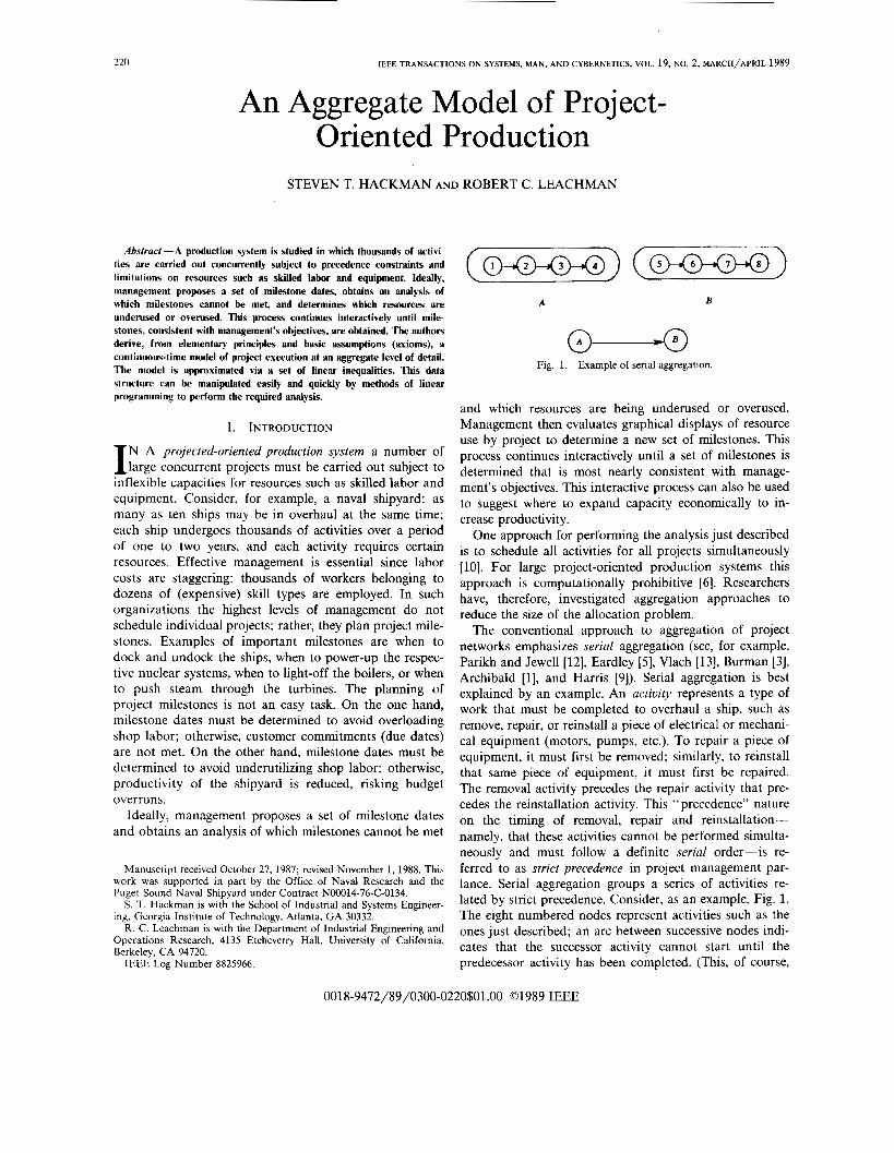
The conventional approach to aggregation of project networks emphasizes serial aggregation (see, for example, Parikh and Jewel1 [12], Eardley [SI, Vlach [13], Burman [3], Archtbald [l], and Harris [9]). Serial aggregation is best explained by an example. An activity represents a type of work that must be completed to overhaul a ship, such as remove, repair, or reinstall a piece of electrical or mechani- cal equipment (motors, pumps, etc.). To repair a piece of equipment, it must first be removed; similarly, to reinstall that same piece of equipment, it must first be repaired. The removal activity precedes the repair activity that precedes the reinstallation activity. This “ precedence” nature on the timing of removal, repair and reinstallation- namely, that these activities cannot be performed simultaneously and must follow a definite serial order-is re- ferred to as strict precedence in project management par- lance. Serial aggregation groups a series of activities related by strict precedence. Consider, as an example, Fig. 1. The eight numbered nodes represent activities such as the ones just described; an arc between successive nodes indicates that the successor activity cannot start until the predecessor activity has been completed. (This, of course,

0018-9472/S9/0300-0220$01 .OO 01989 IEEE

HACKMAN AND LEACHMAN: AGGREGATE MODEL OF PROJECT-ORIENTED PRODUCTION 221

Repair Aggrcgalc Re-install Aggregate A .

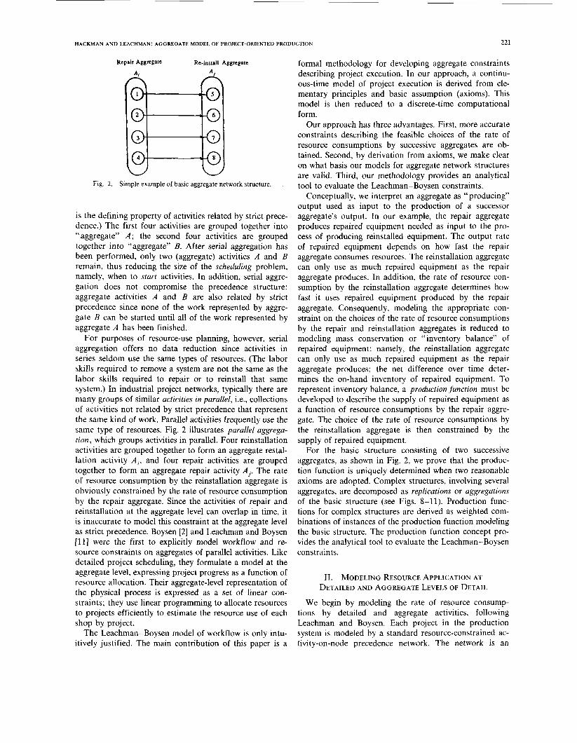
Fig. 2 . Simple example of basic aggregate network structure. ,

is the defining property of activities related by strict precedence.) The first four activities are grouped together into “aggregate” A ; the second four activities are grouped together into “aggregate” B. After serial aggregation has been performed, only two (aggregate) activities A and B remain, thus reducing the size of the scheduling problem, namely, when to start activities. In addition, serial aggregation does not compromise the precedence structure: aggregate activities A and B are also related by strict precedence since none of the work represented by aggregate B can be started until all of the work represented by aggregate A has been finished.

For purposes of resource-use planning, however, serial aggregation offers no data reduction since activities in series seldom use the same types of resources. (The labor skills required to remove a system are not the same as the labor skills required to repair or to reinstall that same system.) In industrial project networks, typically there are many groups of similar activities in parallel, i.e., collections of activities not related by strict precedence that represent the same kind of work. Parallel activities frequently use the same type of resources. Fig. 2 illustrates parallel aggregation, which groups activities in parallel. Four reinstallation activities are grouped together to form an aggregate restal- lation activity A , , and four repair activities are grouped together to form an aggregate repair activity A,. The rate of resource consumption by the reinstallation aggregate is obviously constrained by the rate of resource consumption by the repair aggregate. Since the activities of repair and reinstallation at the aggregate level can overlap in time, it is inaccurate to model this constraint at the aggregate level as strict precedence. Boysen [2] and Leachman and Boysen [ll] were the first to explicitly model workflow and resource constraints on aggregates of parallel activities. Like detailed project scheduling, they formulate a model at the aggregate level, expressing project progress as a function of resource allocation. Their aggregate-level representation of the physical process is expressed as a set of linear constraints; they use linear programming to allocate resources to projects efficiently to estimate the resource use of each shop by project.

The Leachman-Boysen model of workflow is only intu- itively justified. The main contribution of this paper is a

formal methodology for developing aggregate constraints describing project execution. In our approach, a continuous-time model of project execution is derived from elementary principles and basic assumption (axioms). This model is then reduced to a discrete-time computational form.

Our approach has three advantages. First, more accurate constraints describing the feasible choices of the rate of resource consumptions by successive aggregates are obtained. Second, by derivation from axioms, we make clear on what basis our models for aggregate network structures are valid. Third, our methodology provides an analytical tool to evaluate the Leachman-Boysen constraints.

Conceptually, we interpret an aggregate as “producing” output used as input to the production of a successor aggregate’s output. In our example, the repair aggregate produces repaired equipment needed as input to the process of producing reinstalled equipment. The output rate of repaired equipment depends on how fast the repair aggregate consumes resources. The reinstallation aggregate can only use as much repaired equipment as the repair aggregate produces. In addition, the rate of resource consumption by the reinstallation aggregate determines how fast it uses repaired equipment produced by the repair aggregate. Consequently, modeling the appropriate constraint on the choices of the rate of resource consumptions by the repair and reinstallation aggregates is reduced to modeling mass conservation or “inventory balance” of repaired equipment: namely, the reinstallation aggregate can only use as much repaired equipment as the repair aggregate produces; the net difference over time determines the on-hand inventory of repaired equipment. To represent inventory balance, a production function must be developed to describe the supply of repaired equipment as a function of resource consumptions by the repair aggregate. The choice of the rate of resource consumptions by the reinstallation aggregate is then constrained by the supply of repaired equipment.

For the basic structure consisting of two successive aggregates, as shown in Fig. 2, we prove that the production function is uniquely determined when two reasonable axioms are adopted. Complex structures, involving several aggregates, are decomposed as replications or aggregations of the basic structure (see Figs. 8-11). Production functions for complex structures are derived as weighted com- binations of instances of the production function modeling the basic structure. The production function concept provides the analytical tool to evaluate the Leachman-Boysen constraints.

11. MODELING RESOURCE APPLICATION AT DETAILED AND AGGREGATE LEVELS OF DETAIL

We begin by modeling the rate of resource consumptions by detailed and aggregate activities, following Leachman and Boysen. Each project in the production system is modeled by a standard resource-constrained activity-on-node precedence network. The network is an


acyclic directed graph on L nodes. The set of arcs is denoted by the symbol H . An arc from node (activity) I to node (activity) m indicates that activity m cannot start until activity I has finished. Let ES, denote the early-start time for activity I , LS, denote the late-start time for activity I , d , denote the duration of activity I , and let 7,''

denote the total amount of resource k that activity I requires, k = 1,2; a , K . We assume that the LS, are based on a resource-feasible finish time for the project.

At the detailed level, resources are assumed to be consumed by an activity at constant rates between start and finish of the activity. That is, if activity I starts at time S,, ES,< S,Q LS,, then between time S, and time S , + d , activity I loads each resource k at the rate rl(/d, . Let yl(( 7) denote the rate of consumption of resource k at time 7 by activity 1. Our assumptions imply that

where

The function z , ( T ) is called the operating intensity for activity 1. The cumulative intensity Z,(t) = 1; z , (T ) d r measures the fraction of the resources required by activity 1 which has been applied up to time t.

The aggregate level is also modeled by a network of activities labeled A,; . -, A,. Each A , is an aggregation of a number of parallel detailed critical path activities. Each detailed activity 1 is assigned to exactly one aggregate A, , indicated by I E A, . An arc between aggregates A , and A, exists in the aggregate network if an arc ( I , m ) E H exists such that I E A , and m E A,. Hereafter, we shall use the same symbol to denote corresponding functions at detailed and aggregate levels, using the subscripts "1" or "m" for a detailed-level function and using subscripts "i" or " j 7 ' for an aggregate-level function. Functions denoted with capi- tal letters are cumulative functions.

Aggregate activities are formed only if the detailed activities within the aggregate use the same mix of resources: that is, the ratios r;/CIEA,rl( a, are independent of k for all I E A , and all aggregates A,. For each 1 E A , , a, denotes the fraction of the total resources required by aggregate A , consumed by activity 1. For many industrial project networks this requirement is not restrictive. In such networks there are many parallel activities using similar or identical mixes of resources.

We illustrate the aggregation with the simple example shown in Fig. 1. Relevant numerical data are provided in Table I. The four activities that comprise the repair aggregate each utilize the same mix of resources; likewise, the four activities comprising the reinstallation aggregate have in common another mix of resource requirements. In an industrial network there would be tens or scores of parallel repair activities all using the same mix, and tens or scores of reinstallation activities all using some other mix.

TABLE I NUMERICAL DATA FOR AN ILLUSTRATIVE EXAMPLE

Repair Aggregate A, Reinstallation Aggregate A ,

Activity I ES, LS, d, a, Activity m ES, LS, d , a,,,

1 0 6 3 1/4 5 3 9 4 1/3 2 1 4 4 1/3 6 5 8 3 1/4 3 2 6 4 1/3 7 6 10 3 1/12 4 3 5 3 1/12 8 6 8 4 1/3

Let r/' denote the total amount of resource k that aggregate A ; requires, and let y , " ( ~ ) denote the rate of consumption of resource k at time 7 by aggregate A; . Since y,"( 7) = C, E ,,y,"( 7) and by assumption y,"( 7) =

r/ (z , (T) for some operating intensity z,, it follows that y,"( 7) = C, E A,rl(zI( 7). The resource-mix requirement further implies that

where z,( 7) = C, E A,a,z,( 7). Thus when the resource-mix requirement is enforced, an aggregate activity's rates of resource consumptions may be indexed by one profile z , ( T ) which is a convex combination of the intensities of the detailed activities. (Compare ( 3 ) with (l).) Each aggregate operating intensity is induced by a schedule for the detailed activities within aggregate A , . Similar to the detailed intensity function z,( T ) , the cumulative aggregate intensity up to time t , Z , ( t ) = 1; z , ( T ) d 7 , represents the fraction of the total resources required to complete all of the detailed activities within aggregate A , consumed by time t.

Let z," denote the operating intensity for aggregate A , , induced by the late-start schedule, and let z: denote the operating intensity for aggregate A , induced by the early- start schedule. By definition of early- and late-start schedules, all induced Z, satisfy

z,"(t) Q zi(t) < z,E(t), for all t . (4)

The "boundary curves" Z," and Z," provide lower and upper bounds through time on the cumulative use of resources by aggregate A , , given activity durations and project completion times, in the absence of resource constraints. The boundary curves for the repair and reinstallation aggregates are depicted in Fig. 3. Let E, = min, E ,,ES,, and let L, = max, E A,[LS, + d , ] . The interval of time over which an aggregate can be operating (i.e., consuming resources) is given by [ E , , L , ] . In the example [ E, , L , ] = [0,10] for the repair aggregate and [E,, L , ] = [ 3 , 1 3 ] for the reinstallation aggregate. For each aggregate A , it is assumed that Z,E(t) > Z,"(t) for all t E ( E , , L,) .

HACKMAN AND LEACHMAN: AGGREGATE MODEL OF PROJECT-ORIENTED PRODUCTION

~

223

0.5

0 1 2 3 4 5 b 7 8 9 10 1 1 1 2 1 3

( a)

time

1.0

0.5

time 0 1 2 3 4 5 b 7 8 9 1 0 1 1 1 2 1 3

(b)

Fig. 3. Boundary curves for illustrative example.

111. A STRUCTURED FORMAL DEVELOPMENT OF AN AGGREGATE MODEL

Even before capacities of resources are considered, the feasible choices for intensities of the aggregate activities are limited. In the example it is obvious that the feasible choices for the rate of resource consumptions by the repair and reinstallation aggregates are dependent, i.e., the choice Z,, for operating the repair aggregate restricts the choice Z, for operating the reinstall aggregate. The strict precede&e model of critical path methods (CPM) insists that resource consumptions by predecessors must be complete before resource consumptions by follow-on activities may commence. Since the periods of operation of the repair and reinstallation aggregates typically overlap, a different model of workflow must be developed.

A . Formulation of the Aggregate Activity Dependence Relationships

Our structured approach characterizes the problem of developing a dependence relationship between A , and A, as a problem of developing a dynamic production function mapping the rate of resource consumptions by A , into outputs from A , , and then expressing conservation through time of the product produced by A , and used as input by A,. To make our approach clear, we first reformulate the resource-constrained CPM as a model of production, whereby strict precedence between two detailed activities is expressed as a form of inventory balance, as follows. For

each activity 1 let U, denote the set of all possible intensity functions, i.e., those defined by (2) with ES, G S, G LS,, and let 2, denote the corresponding set of all possible cumulative intensities. For each (1, m ) E H define f , ( ' * m ) :

U, -+ U, as

if r E ( S , + d , , S, + d , + d , ) otherwise.

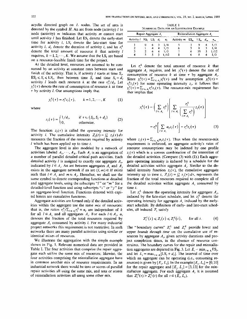
(Clarifying the notation, z , and f , ( ' - " ) ( t , ) are both functions of time. f / ' ,") (z , ) ( r ) denotes the value of the latter function at time 7.) Referring to Fig. 4(a) the functional f i ( r * m ) maps the intensity curve for activity 1 into the earliest intensity for activity m consistent with the assumption of strict precedence. Let F,">")(t) = /d f / ' , m ) ( z , ) ( T ) d r denote the cumulative function corresponding to f,(" ")( z , ) . The constraint

F,".")(Z,)(t) 2 z,(t), for all t ( 5 )

is mathematically equivalent to the requirement that S, + d , G S,. See Fig. 4(b). Thus ( 5 ) expresses strict precedence via a functional relationship between the resource consumptions by 1 and m indexed by z , and z,, respectively. From the perspective of dynamic production theory ([SI), (5) has a natural interpretation as an inventory balance constraint: f / l , m ) ( z r ) is a (dynamic) production function representing the "output" of intermediate product "(l,m)" by activity I , and z , represents the application of intermediate product ( I , rn) by activity m .

Conceptually, our model of resource use at the aggregate level parallels our model of resource use at the detailed level. We view aggregate activities as producing intermediate products used by follow-on aggregate activities. Pro- duction by an aggregate activity is explicitly modeled via a (dynamic) aggregate production function F,(, , '): 2 , -+ 2, similar in spirit to F/'v")(Z,). The feasible set of choices for resource consumptions by aggregate activities A , and A, is expressed via the inventory balance constraint

F,(fv')(Z,)(t) >, z,(t), for all t (6)

similar in spirit to (5). Throughout the remainder of this section we suppress the superscript ( i , j ) and denote F,('.''(Z,) by F,(Z,) .

The ideal choice for F, (Z,) is given by

I E A ,

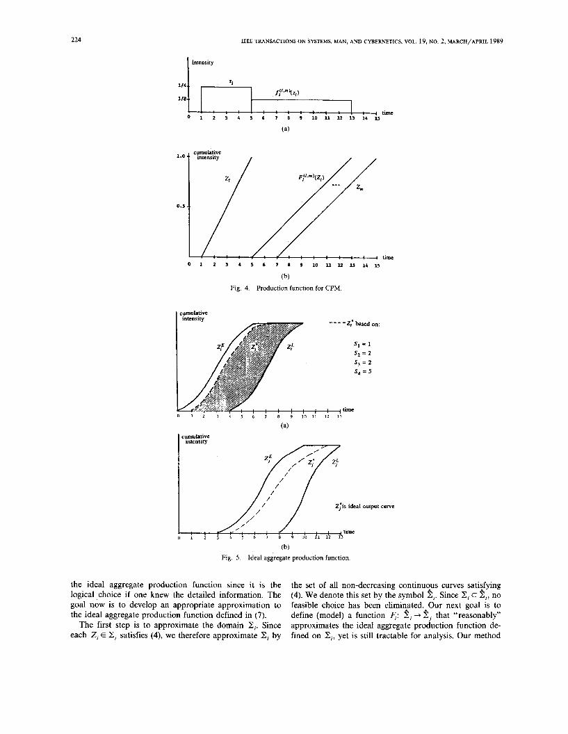
Equation (7) is precisely the cumulative aggregate operating intensity for A, induced by the earliest schedule for the activities within A, consistent with the finish times for the activities in A , that precede them. Fig. 5(b) shows the ideal output curve corresponding to the input curve Z,* shown in Fig. 5(a). Unfortunately, the model for F, given in (7) is unworkable: it incorporates knowledge of the schedules (start times) for the activities within A, . A model for the aggregate production function must be independent of such knowledge so as not to defeat the whole point of aggregation. We shall refer to the function defined in (7) as

224 IEEE TRANSACTIONS ON SYSTEMS, MAN, AND CYBERNETICS, VOL. 19, NO. 2 , MARCH/APRIL 1989

intensity I

time 0 1 1 3 4 5 6 7 8 9 1 0 1 1 l Z l 3 1 4 U

(b)

Fig. 4 . Production function for CPM.

I cumulative

s, = 2

s, = 2 s, = 5

0 1 2 3 4 5 6 7 8 9 1 0 1 1 1 2 1 3

(a)

cpnulative mtensity

Z;is ideal output curve

(b) Fig. 5. Ideal aggregate production function.

the ideal aggregate production function since it is the logical choice if one knew the detailed information. The goal now is to develop an appropriate approximation to the ideal aggregate production function defined in (7).

The first step is to approximate the domain 2,. Since each 2, E 2, satisfies (4), we therefore approximate Z, by

the set of all non-decreasing continu2us curves sati!fying (4). We denote this set by the symbol 2,. Since Z, C Z,, no feasible choice has been elimi\ated.AOur next goal is to define (model) a function 4: Z , 4 Z, that “reasonably” approximates the ideal aggregate production function defined on Z,, yet is still tractable for analysis. Our method


I cumulative

time 0 1 2 3 4 5 6 7 8 9 1 0 1 1 1 2 1 3

(a) cumulative

mtensity

0 1 z 3 4 5 6 7 8 9 1 0 1 1 1 2 1 3

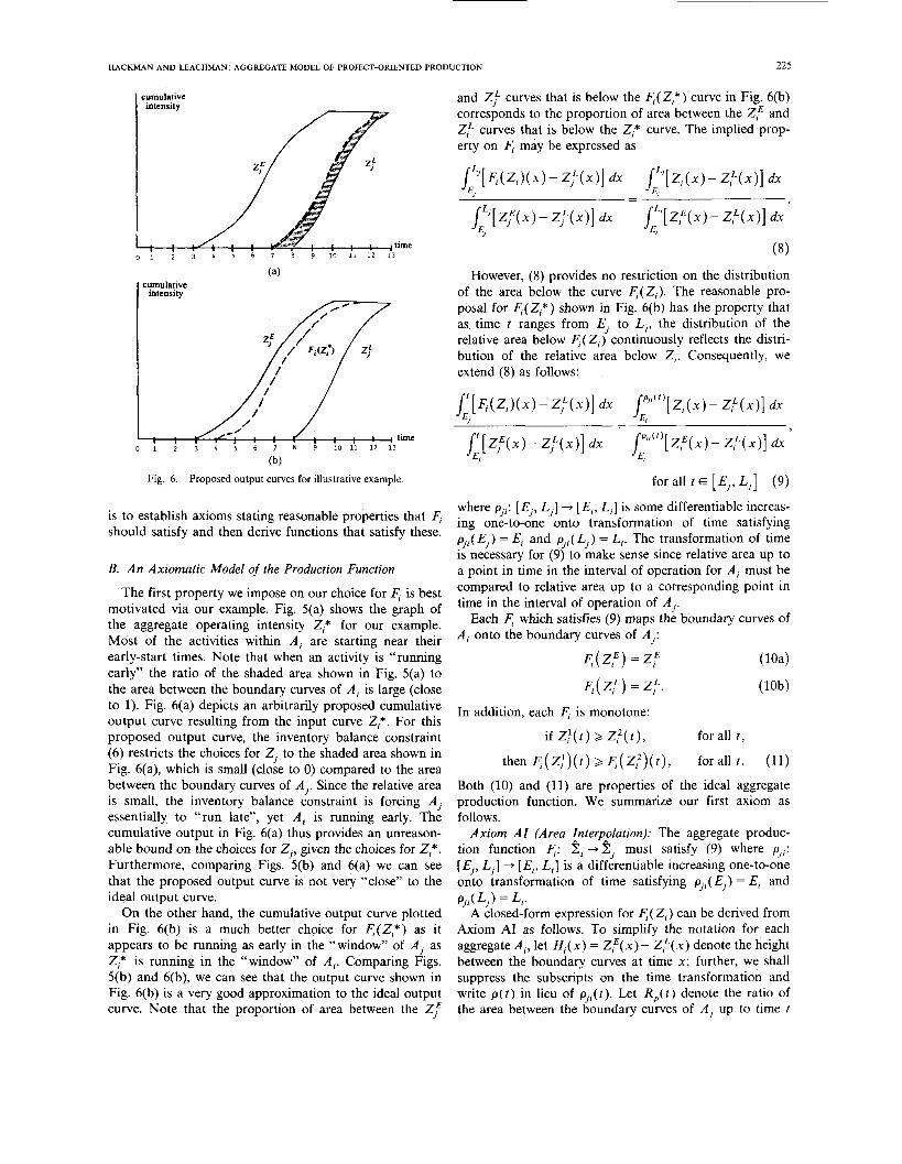
(b) Fig. 6 . Proposed output curves for illustrative example.

is to establish axioms stating reasonable properties that F, should satisfy and then derive functions that satisfy these.

B. An Axiomatic Model of the Production Function

The first property we impose on our choice for F, is best motivated via our example. Fig. 5(a) shows the graph of the aggregate operating intensity Z,* for our example. Most of the activities within A , are starting near their early-start times. Note that when an activity is "running early" the ratio of the shaded area shown in Fig. 5(a) to the area between the boundary curves of A , is large (close to 1). Fig. 6(a) depicts an arbitrarily proposed cumulative output curve resulting from the input curve Z,*. For this proposed output curve, the inventory balance constraint (6) restricts the choices for Z, to the shaded area shown in Fig. 6(a), which is small (close to 0) compared to the area between the boundary curves of A,. Since the relative area is small, the inventory balance constraint is forcing A, essentially to "run late", yet A , is running early. The cumulative output in Fig. 6(a) thus provides an unreason- able bound on the choices for Z,, given the choices for Z,*. Furthermore, comparing Figs. 5(b) and 6(a) we can see that the proposed output curve is not very "close" to the ideal output curve.

On the other hand, the cumulative output curve plotted in Fig. 6(b) is a much better choice for F,(Z,*) as it appears to be running as early in the "window" of A, as Z,* is running in the "window" of A , . Comparing Figs. 5(b) and 6(b), we can see that the output curve shown in Fig. 6(b) is a very good approximation to the ideal output curve. Note that the proportion of area between the Z/"

and Z: curves that is below the F,(Z,*) curve in Fig. 6(b) corresponds to the proportion of area between the Z," and Z," curves that is below the Z,* curve. The implied property on F, may be expressed as

/" ' [Z ," (x ) - Z,"(x)] dx / L ' [ Z p ( x ) - Z : ( x ) ] dx E, E,

(8)

However, (8) provides no restriction on the distribution of the area below the curve F, (Z , ) . The reasonable pro- posal for F,(Z,*) shown in Fig. 6(b) has the property that as time t ranges from E, to L,, the distribution of the relative area below I;; ( Z , ) continuously reflects the distribution of the relative area below Z , . Consequently, we extend (8) as follows:

/ E ~ f ( ' ) [ Z , ( x ) - Z , " ( x ) ] dx

for all t E [E,, L,] (9)

where p,,: [E,, L,] - [E, , L,] is some differentiable increasing one-to-one onto transformation of time satisfying p,, (E,) = E, and p,, (L,) = L,. The transformation of time is necessary for (9) to make sense since relative area up to a point in time in the interval of operation for A , must be compared to relative area up to a corresponding point in time in the interval of operation of A,.

Each F, which satisfies (9) maps the boundary curves of A , onto the boundary curves of A,:

F , ( Z E ) = ZJ"

F,(z,") =z;. In addition, each F, is monotone:

if Z, ' ( t ) 2 Z: ( t ) , for all t ,

then F , ( Z , ' ) ( t ) 2 F , ( Z : ) ( t ) , for all t . (11)

Both (10) and (11) are properties of the ideal aggregate production function. We summarize our first axiom as follows.

Axiom A I (Area !nterpflation): The aggregate production function 4: 2, +Z, must satisfy (9) where p,,: [E, , L,] - [E, , L,] is a differentiable increasing one-to-one onto transformation of time satisfying p,, ( E , ) = E, and

A closed-form expression for F,( Z , ) can be derived from Axiom AI as follows. To simplify the notation for each aggregate A , , let H, ( x ) = Z,"( x ) - Z,"( x ) denote the height between the boundary curves at time x ; further, we shall suppress the subscripts on the time transformation and write p ( t ) in lieu of p , , ( t ) . Let R , ( t ) denote the ratio of the area between the boundary curves of A , up to time t

P,,(L,) = L,.


to the area between the boundary curves of A ; up to time p ( t ) , i.e.,

Upon rearrangement (9) becomes

F, ( z, ) ( x ) dx = ZF( x ) dx + R , ( t ) t, JE,

cumulative I intensity

0 1 2 3 0 5 6 7 8 9 1 0 1 1 1 2 1 3

(a)

- [ ( " ' { Z i ( x ) - Z ~ ( x ) } d x 1 . (13)

Differentiate each side of (13) with respect to t to obtain

F , X Z ; ) ( d = z,"<t>+ R p ( t > { Z , ( p ( t ) ) - Z , L ( P ( t ) ) ) P ' ( t )

+ R;W[ J - ' " ( z J ( x ) - Z W ) d x ] (14)

time where 0 1 2 3 4 5 6 7 8 9 1 0 1 1 1 2 1 3

P,,(9) = 5.6

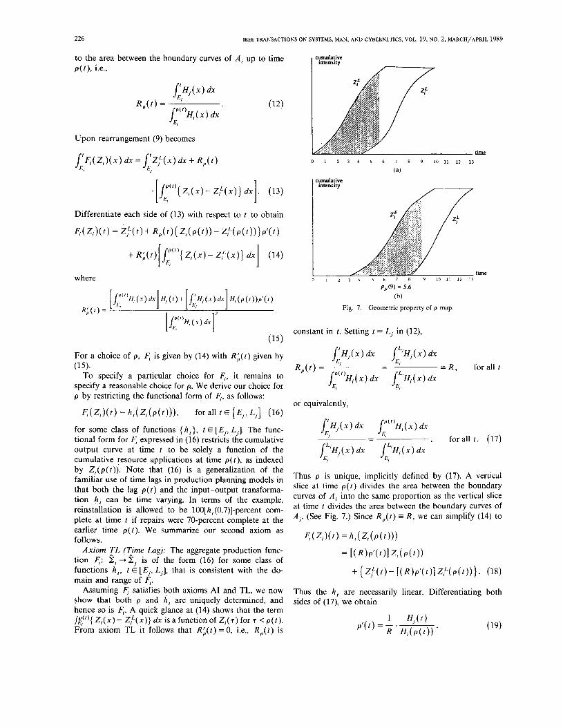
(b) [ J;(% (.> d. H/ ( 1 ) + Ir H, dx H, ( P ( f ) ) P ' ( f ) RL(f) = 1 [ E , 1 Fig. 7. Geometric property of p map.

constant in t. Setting t = Lj in (12), (15)

[ p4 (XI dx- I' For a choice of p, c. is given by (14) with R;( t ) given by (15). R , ( d =

dx J L I H j ( x ) dx

= R , for all t E/ - - To specify a particular choice for F,, it remains to

specify a reasonable choice for p. We derive our choice for p by restricting the functional form of F,, as follows:

F ; ( Z ; ) ( t ) = h , ( Z , ( p ( t ) ) ) , forall [E j ,L , ] (16)

J P % ; ( X ) dx J L , H ; ( x ) dx

J;,H,(x) dx J P ( % ; ( X ) dx

E, E,

or equivalently,

for some class of functions { h t } , t E [E,, L,]. The func-

cumulative resource applications at time p ( t ) , as indexed J E,

tional form for F, expressed in (16) restricts the cumulative output curve at time t to be solely a function of the

- - E, , for all t . (17)

lELIH, ( x ) dx /'*'Hi( x ) dx

by Z , ( p ( t ) ) . Note that (16) is a generalization of the familiar use of time lags in production planning models in that both the lag p ( t ) and the input-output transformation h , can be time varying. In terms of the example, reinstallation is allowed to be 100[ hf(0.7)]-percent complete at time t if repairs were 70-percent complete at the

Thus p is unique, implicitly defined by (17). A vertical slice at time p ( t ) divides the area between the boundary curves of A , into the same proportion as the vertical slice at time t divides the area between the boundary curves of A,. (See Fig. 7.) Since R , ( t ) = R , we can simplify (14) to

earlier time p ( t ) . We summarize our second axiom as follows. F , ( Z , ) ( t ) = h , ( Z , ( P ( t ) ) )

= [ ( R ) P ' ( t ) l Z f ( P ( t ) ) Axiom TL (Time Lag): The aggregate production function F,: Z, + 2, is of the form (16) for some class of

main and range of 4. Satisfies both axioms AI and TL, we now

show that both p and h , are uniquely determined, and hence so is F, . A quick glance at (14) shows that the term

functions h,, t E [E,, L,], that is consistent with the do- + (z;<t>- [ ( R ) P ' ( t ) l Z , " ( p ( t ) ) ) . (18)

Assuming Thus the h , are necessarily linear. Differentiating both sides of (171, we obtain

(19) /$"{ Z , ( x ) - Z ,L (x ) } dx is a function of z , ( T ) for T < p( r> . From axiom TL it follows that R;( t ) = 0, i.e., R,(t) is

1 H , ( d R H , ( P ( t ) ) .

p ' ( t ) = - .


Substituting (19) into (18), F , ( ' . j ) ( Zi)( t )

for all t , (20) and then substituting (20) into the inventory balance constraint (6) yields

, for all t . Z , ( P , k ) ) - Zl"(P, , ( t ) ) ~ z,W- Z ; ( d

HI ( P,, ( t )> H , ( t ) (21)

We summarize our model development with the following Theorem.

Theorem: If F,('*'): 2, -+ 2, satisfies Axioms A I and TL, then <(',') is uniquely defined by (20) where p,, is implicitly defined by (17).

C. Remarks

The dependence constraint proposed for the basic aggregate network structure studied in this section is (21), which implicitly defines an aggregate production function I;; (18) satisfying axioms AI and TL. Fig. 6(b) depicts the cumulative output curve corresponding to this production function. As noted earlier, a comparison of Figs. 5(b) and 6(b) shows that F,( Z,* ) is very close to the ideal output curve.

To develop a computational form for the model expressed in (21), we divide time into discrete intervals (O, l ] ; . . , ( t - l , t ] , . . . , (T- l ,T] and define intensity variables z,(T) representing a constant intensity rate for A , during the interval ( 7 , ~ - 11. We enforce (21) at the integer points in time. The constraint (21) can be expressed in terms of the discrete-time variables as follows. For a real number x , let x + denote the smallest integer greater than or equal to x , and let x - denote the largest integer less than or equal to x . Each Z , is a piecewise-linear curve, expressed in terms of the variables as

t -

z,(t) = c z , < . > + < t - t - > { Z , < t + > > . 7-1

It may be readily verified that

z:( t ) = z;( t - ) + ( t - t - ) { z:( t + ) - z," ( t - ) } ,

H , ( t ) = H , ( t - ) + ( t - t - ) { H , ( t + ) - H , ( t - ) } .

and similarly,

To compute p,,(t), let

p,w dx A , ( t ) =

/"H, ( x ) dx E,

denote the relative area between the boundary curves of A, . By assumption H , ( x ) is strictly positive on ( E , , L,), so that the curve A , ( t ) is strictly increasing on (E , , L,) and

hence has an inverse. The implicit definition (171 1 Jr p,, is simply the statement that p,,(t) = A,-l(A,(r)) . It may be readily verified that

A , ( d = A h - )

( t - t - ) H , ( t - ) + 1/2(t - t - )'[ H, ( t + ) - H , ( t - ) ]

/"'HI (x) dx +-

E,

(22 If A l ( t ) and A , ( t ) are precomputed for all integer t , then given an arbitrary t the corresponding time point p,,( t ) for which A, (p , , ( t ) ) = A , ( t ) can be easily computed using (22). By precomputing Z,"(t), Z;(t) , H , ( t ) , H , ( t ) , and p,,(t) for all integer t , linear inequalities in the z,(7) variables can be constructed to enforce (21).

We note that it is not necessary that F, (Z , ) satisfy both axioms AI and TL for it to be computationally practical. The area interpolation axiom (14) reduces to a linear expression for F,(Z,)(t) in terms of the variables z,(l), z,(2),. * e , z,(p,,(t)-), z,(p,,(t)+). (The weights of the lin-

ear expression are nonlinear functions of t . ) If axiom TL is not adopted, then by the theorem we know that some p,, other than (17) must be specified.

Even if the detailed arcs from A , to A, do not provide a one-to-one correspondence between detailed activities in A , and A,, the model for F, (Z , ) expressed in (20) still applies. In fact, the model for F,(Z, ) does not preclude strict precedence among detailed activities within an aggregate. However, the resource-mix requirement typically would not hold for such aggregation.

Finally, we remark that both axioms are testable. For various intensities Z, E Z, one could measure how F, (Z , ) deviate from the ideal output curve. In limited simulation experiments, Dalebout [4] shows that the model performs reasonably well. In general, simulation tests conducted a priori could provide a means of evaluating whether or not an acceptable aggregation of a project network structure has been performed.

IV. MORE COMPLEX AGGREGATE SUBNETWORKS

In this section we develop the inventory balance constraints of the aggregate model for more complex network structures. We demonstrate that various aggregate network structures may be viewed as replications or aggregations of the basic aggregate network structure.

A . Replicated Network Structures

Consider the subnetwork shown in Fig. 8(a). The task here is to determine a set of constraints that serves to constrain the possible choices for Z, given choices for Z , and Z,. To develop the set of constraints we construct an equivalent network structure and analyze it instead. Con- sider Fig. 8(b). It is obtained by replicating aggregate 3 so that we have aggregates A , and A,,. The precedence constraints for the network system in Fig. 7(b) are identical to the original precedence constraints. Note that Fig.

228 IEEE TRAXSACTIONS ON SYSTEMS, MAN, AND CYBERNETICS, VOL. 19, NO. 2, MARCH/APRIL 1989

Fig. 8. Replicated aggregate network structure: Case of multiple predecessors.

8(b) consists of two examples of the basic aggregate network structure discussed in Section 111. Hence inventory balance constraints for the aggregate subnetwork shown in Fig. 8(b) are

F{193’( z,) 2 z3 (234

~ p 3 y 2,) > z, (23b)

z, = Z3?. (234 We add (23c) to ensure that aggregates A , and A3, are identically operated.

Substituting (23c) into (23b), we see that the inventory balance constraints governing the structure in Fig. 8(a) must be

F/1,3)( z , ) >, z3 (244

F2’233’( z,) 2 z3. (24b) From (24) we see that aggregate A , requires two distinct intermediate product inputs, one from aggregate A , and the other from aggregate A,. We remark that the derivation of the abstract system (24) is independent of the choice for the basic aggregate production function. Substi- tuting into (24) our choice (21) for the basic aggregate production function, constraints (24) become

Next, consider the network structure shown in Fig. 9(a). Proceeding exactly as before, we replicate aggregate A,, obtaining the subnetwork shown in Fig. 9(b) with aggregates A , and A,,. The system of constraints for the equiva-

A I A2

A i 1-1 A3

(b)

Fig. 9. Replicated aggregate network structure: Case of multiple successors.

lent network is

F{’J’( z,) > z, (264

F$”33’( z,) > z3 (26b)

2, = Z,L (264 Following our earlier argument, the constraints for the network system in Fig. 9(b) must be

F{’J’( z,) 2 z, (274

F{’*3’( z ,) > z3. (27b) From (27) we see that aggregate A , produces two distinct intermediate products, one for aggregate A , and the other for aggregate A, . The derivation of (27) makes no assumption about the choice for the aggregate dynamic production function. Substituting our choice (21), the constraints become

(284 z,(d - Z2L(t) Z l ( P 2 l ( t ) ) - z l%21( t ) )

2 H 2 ( d Hl( P21(t))

z 3 ( t ) - z : ( t ) z 1 ( P 3 1 ( t ) ) - Z : . ( P 3 1 ( f ) ) . (28b) >,

H 3 ( t ) H l ( p31( 1) B. Aggregations of the Basic Aggregate Network Structure

We now consider the network structure shown in Fig. 10(a). Here the task is to develop a set of constraints modeling the possible choices for Z3, given the choices for Z , and Z,. Compare Fig. 10(a) to Fig. 8(a): at the aggregate level the subnetworks appear to be the same; at the detailed level they are fundamentally different. In Fig. 10(a) each detailed activity within aggregate 3’ receives input from a detailed activity within aggregates 1 or 2 but not both, in contrast to the network in Fig. 8(a). The

HACKMAN AND LEACHMAN: AGGREGATE MODEL OF PROJECT-ORIENTED PROD IUCTION 229

A2 A3

I

A I

A2 \ # *- -‘

(b)

predecessors. Fig. 10. Aggregation of basic structures: Case of multiple

outputs of aggregates 1 and 2 are used by different por- tions of aggregates 3’. A set of constraints other than (24) must be developed.

Consider Fig. 10(b). Aggregates A , and A , are the subaggregates of A , whch use input from aggregates A , and A,, respectively. From the perspective of Fig. 10(b) the subnetwork in Fig. 10(a) can be viewed as the result of sequential aggregation. First, aggregates A,, A, , A , , and A , were formed; second, aggregates A , and A , were further aggregated into “super” aggregate A,,. If the second iteration had not been performed, then the system of constraints for the first level of aggregation would have been

F,“93’( z ,) 2 z, (294

F2’2*4’( z,) 2 z,. (29b) By aggregating a second time we no longer know how Z,, is decomposed into Z , and Z,. (If we knew this information, then we would just use (29).) We must, therefore, constrain the choices for Z,, as a function of the output curves F11s3) and F2(2*4).

Let a, and a, denote subaggregate A,’s and A,’s per- centage of the total resources required by super-aggregate A3,, respectively. It may be readily verified that ea$h Z,, E 5,. is expressible as a , Z , + a4Z, for some Z , E E,, Z , E 2,. We convexify the constraints (29a) and (29b) in the obvious way to obtain

a,F,(’33)( z,) + a,F2(294)( z,) >, Z,!. (30) Every choice for Z,, Z, , Z,, and Z, feasible in (29) will be feasible in (30). For this reason we use (30) to model the dependence relationships for the subnetwork shown in Fig. 10(a). Constraint (30) may be interpreted as follows: ag-

‘ - - e ’ (b) Fig. 11. Aggregation of basic structures: Case of multiple successors.

gregates A , and A , produce the same product which is input by superaggregate A,,; the total supply of this product from A , and A , determines the progress that can be made by A3,.

As before, the resulting inventory balance constraint is independent of the choice for the basic production function. Substituting our choice (21) into (30) and simplifying, we obtain

Note that when a3 = 1, H3( t ) = H,.( t ) and a, = 0, so that (31) reduces to the inventory balance equation for a basic aggregate subnetwork, as expected.

Next, we consider the network structure shown in Fig. ll(a), the apparent “dual” to Fig. 10(a). Referring to Fig. ll(b), we can view Fig. ll(a) as having been obtained via sequential aggregation: first, aggregates A, , A , , A , , and A , were formed, and second, aggregates A , and A , were aggregated into a superaggregate A,,. As before, if the second iteration had not been performed, the inventory balance constraints would be given by (29). Since the second iteration was performed, we have no knowledge of how Zr is decomposed into Z , and Z,. Once again we

230 IEEE TRANSACTIONS ON SYSTEMS, MAN, AND CYBERNETICS, VOL. 19, NO. 2, MARCH/APRIL 19R9

must combine constraints (29a) and (29b) in some logical way.

Since the arguments of the production functions F$'*,), are no longer known, it is not possible to "add" these two functions (as in the previous case) without specifying the functional form for the basic aggregate production function. Substituting our choice (20) into (29), we write

In (32) we have written the balance constraints in terms of the inverses of the time transformation maps to present the same time arguments in the functions for A , as in the functions for A,. Proceeding as before, we let a1 and a2 denote the fraction of total resources consumed by A I , which are applied to subaggregates A , and A , , respectively. Noting that a , Z , + a 2 Z , = Z,, we combine (32a) and (32b) to obtain

a , H , ( t ) Z , ( f , ' ( t > ) - Z,"(P,'(t>)

H I 4 4 -.

H3 ( P i 1 ( t )

a , H 2 ( t ) 4 4 t )

Z 4 ( p G 1 < d 1 - Z4L(PG1(t))

H,(P4ad)

+-

Z1!( t ) - z;( t )

' Hl,( t ) (33)

When a, = 1, H , ( t ) = H , , ( t ) and a2 = 0, so that (33) reduces to the inventory balance equation for a basic aggregate subnetwork, as expected. Constraint (33) may be interpreted as follows: superaggregate A,. produces one intermediate product that is a shared input to aggregates A , and A,; the total consumption of this product by A , and A , determines the progress of A,, required to support their activity.

v. COMPARISON TO THE LEACHMAN-BOYSEN MODEL

Leachman and Boysen [ll] propose aggregate activity dependence relationships expressed in terms of the "relative earliness" of the aggregates. For t E [E;, L j ] they define the relative earliness of Ai as

For the basic aggregate network

t = E,

E , < t < L, (34)

t = L,.

structure in which A ,

precedes A,, they require for each t E [E,, L,] that

P , ( f / , W ) 2 P , W (35)

where p,,(r) is chosen as the time point in [E,, L,] which "corresponds" to time point t E [E, , L,] in the following sense. A vertical slice at time p, , ( t ) divides the area between the window curves of A , into proportions the same as a vertical slice at time t divides the area between the window curves of A,.

For more complex structures which are decomposable into replications of the basic aggregate network structure, multiple constraints of the form (35) are proposed; for structures that are aggregations of the basic aggregate network structure, constraints are proposed of the form

i

or

1

where (36) applies in the case that subaggregates of A, are preceded by different aggregates and where (37) applies in the case that subaggregates of A , are succeeded by different aggregates. The coefficients c,, and a,, are constants expressing the relative requirements of the subaggregates.

The Leachman-Boysen constraint (35) is identical to (21), utilizing the same p map. Their constraints in the case of replicated structures also coincide with our derived constraints. However, the Leachman-Boysen constraints are not the same as our derived constraints in the case of aggregated structures. In terms of relative earliness, our constraint (31) may be rewritten as

Since a 3 H 3 ( t ) + a 4 H , ( t ) = H3'(t), (38) reveals that in our model the relative earliness of A,, at time t is bounded by a time-varying convex combination of the relative earliness of A , and of A , at respective time points ~ 3 1 ( t ) , p42(t). Comparing our model to (36), we see that Leachman- Boysen uses constant weights, which are more approximate; moreover, they use p,.,( t ) , pY2( t ) instead of p31( t ) , p42(t) . Essentially, our model would reduce to the Leach- man-Boysen model only if subaggregates A , and A , were identical.

In terms of relative earliness, our constraint (33) may be rewritten as

Since a,H,(r )+ a , H , ( t ) = H,, ( t ) , (39) reveals that in our model the relative earliness of A,' bounds a time-varying convex combination of the relative earliness of A , and of A , at respective time points p<'(t), p z l ( t ) . Comparing to

HACKMAN AND LEACHMAN: AGGREGATE MODEL OF PROJECT-ORIENTED PRODUCTION

(37), once again we find that Leachman-Boysen uses constant weights, which are more approximate; moreover, once again they use different p maps. Essentially, our model reduces to the Leachman-Boysen model only if subaggregates A , and A , are identical.

VI. A LINEAR PROGRAMMING APPROACH TO MULTIPROJECT PLANNING

Constraints of the form (4), (21), (31), and (33) serve to restrict the possible choices for the intensities (i.e., the resource applications) of the aggregate activities of each project. Adding standard resource capacity constraints, the overall set of constraints is expressed as a set of linear constraints on discrete-time intensity variables for each aggregate activity of each project. The set of constraints models the set of feasible resource allocations to the projects. Using an appropriate objective function (for example, discounting the underutilization of existing capacities to maximize productivity), a linear program can be solved to compute resource allocations. Management would then evaluate the resource allocations to determine a new set of milestone dates.

VII. CONCLUSION

An aggregate model of project-oriented production has been developed for use in multiproject resource allocation. The model has been derived from reasonable axioms con- cerning the production function of an aggregate and from basic principles such as inventory balance and resource conservation. By defining basic assumptions and proceeding formally, we obtain improvements to a previously proposed aggregate model.

We remark that the three-phase approach of elevating a model from a computational form to a continuous-time framework, rigorously analyzing it relative to basic assumptions and elementary principles, and then restoring it to a computational form can improve production models in many contexts. Even simple familiar models, such as standard linear programming formulations with time lags, material requirements planning, and critical path scheduling, can be reformulated more accurately or more gener- ally with this approach. See Hackman and Leachman [8].

ACKNOWLEDGMENT

The authors would like to thank their colleagues John J. Bartholdi 111, King-tim Mak, Loren K. Platzman, Craig A. Tovey, and John H. Vande Vate for insightful comments on earlier drafts. We would also like to thank the referees for constructive comments. A portion of the material in this paper was adapted from Hackman [7, ch. 41.

~

231

REFERENCES

R. D. Archibald, Managing High-Technology Programs and Pro- jects. New York: Wiley, 1976. J. Boysen, “An aggregate project model for resource allocation within multiproject construction systems,” Ph.D. Thesis, Dept. Ind. Eng. and Oper. Res., Univ. CA, Berkeley, 1982. P. J. Burman, Precedence Networks for Project Planning and Con- trol. New York: McGraw-Hill, 1972. D. Dalebout, “A study of dependence relationships between aggregate activities in a project-oriented production system,” M.S. thesis, Dept. Ind. Eng. and Oper. Res., Univ. of CA, Berkeley, 1983. V. J. Eardley, “Production of multi-level critical path networks,” Ph.D. thesis, Dept. Civil Eng., Univ. of IL, Urbana, 1969. M. R., Garey and D. S. Johnson, Computers and Intractability: A Guide to the Theory of NP-Completeness. San Francisco: W. H. Freeman and Co., 1979. S. T. Hackman, “A general model of production: Theory and application,” ISyE Report C-84-2, School of Ind. and Syst. Eng., GA Inst. of Tech. S. T. Hackman and R. C. Leachman, “A general framework for modeling production,” ORC Rep. 86-9, Eng. Syst. Res. Center, Univ. of CA, Berkeley, revised 1987, to appear in Management Sci. R. B. Harris, Precedence Arrow Networking Techniques for Construc- tion. New York: John Wiley, 1978. I. Kurtulus and E. W. Davis, “Multiproject scheduling: Categoriza- tion of heuristic rules performance,” Munagement Sci., vol. 28,

R. C. Leachman and J. Boysen, “An aggregate model for multiproject resource allocation,” in Project Manugement: Methods and Studies, B. V. Dean, Ed. Amsterdam: North Holland,

S. C. Parikh and W. S. Jewell, “Decomposition of project networks,” Munugement Sei., vol. 11, pp. 444-459, 1965. J. Vlach, “Some results of connecting (aggregating) networks in building,” in Internet 2: Project Planning by Network Analysis. Amsterdam, The Netherlands: North Holland, 1969, pp. 418-426.

pp. 161-172,1982.

pp. 43-64, 1985.

Robert C. Leachman received the B.A. degree in mathematics and physics, and the M.S. and Ph.D. degrees in operations research from the Univer- sity of California, Berkeley.

He is currently Associate Professor of Indus- trial Engineering and Operations Research at the University of California, Berkeley. He is a con- sultant to many manufacturing firms, including several leading semiconductor manufacturing firms. His research interests include dynamic production theory, production planning and

Dr. Leachman is a member of ORSA/TIMS. He is also an Associate scheduling, project scheduling, and railroad operations analysis.

Editor of the Journal of Munufaciuring Systems.

Steven T. Hackman received the B.S. degree in industrial engineering and operations research from Cornell University, Ithaca, NY, and the M.A. degree in mathematics, and the M.S. and Ph.D. degrees in operations research from the University of California, Berkeley.

He is currently Assistant Professor of Indus- trial and Systems Engineering at the Georgia Institute of Technology, Atlanta. His research interests include production planning and production theory, applied production analysis, ma-

terial handling, and mathematical programming. Dr. Hackman is an Associate Editor of Operations Research and the

Journal of Productivity Ana!vsis. He is a member of ORSA/TIMS and IIE.

An aggregate model of project-oriented production

Documents

Transcript of An aggregate model of project-oriented production