AGGREGATE PRODUCTION PLANNING MODELS

INCORPORATING DYNAMIC PRODUCTIVITY

By

BEHROKH KHOSHNEVIS ~

Bachelor of Science Arya-Mehr University of Technology

Tehran, Iran 1974

Master of Science Oklahoma State University

Stillwater, Oklahoma 1975

Submitted to the Faculty of the Graduate College of the Oklahoma State University

in partial fulfillment of the requirements for the Degree of

DOCTOR OF PHILOSOPHY December, 1979

.. ·

AGGREGATE PRODUCTION PLANNING ·MODELS

INCORPORATING DYNAMIC PRODUCTIVITY

Thesis Approved:

Dean of the Graduate College

ii

PREFACE

This research incorporates the effects of the dynamic productivity

phenomena present in most industrial situations into the aggregate

planning problem. The research originates the introduction of the

effect of disruptions in productivity improvement, progress and retro­

gression to this production and workforce planning area. Aggregate

production planning of both long cycle and short cycle product situa­

tions are considered and models peculiar to each case are developed and

analyzed. The new models are shown to have significant economic impact

in the majority of situations.

The general solution methodology utilized in this research was

developed by W. H. Taubert [65]. Chapter IV of this research presents

a summary of this methodology and contains a number of quotes from his

work. The analysis of the manpower disruption effects presented in

earlier parts of Chapter V draws heavily from the original efforts of

E. B. Cochran [19]. With his permission, quotes from his work are used

in this chapter.

I wish to express my most sincere thanks to my uncle, Mr. Ali

Khoshnevis, for his unending devotion and faith which have enriched and

strengthened me throughout my life.

I wish to convey my special appreciation to Dr. Philip M. Wolfe,

who served as an excellent research adviser during the course of this

work. Without his inspiration, guidance and encouragement this program

would not have been completed. I also appreciate his personal concern

iii

for my career.

A very special acknowledgment must be given to Dr. Joe H. Mize,

the Head of the Department of Industrial Engineering and Management,

for his excellency in the academic area and in leadership. His belief

in my abilities and delegation of teaching and research responsibilities

have inspired my self-realization and confidence.

I extend my sincere thanks to Dr. Marvin P. Terrell, the chairman

of my Ph.D. committee, Dr. Hamed K. Eldin and Dr. Donald W. Grace, who

served as members of my committee.

To my mother and brothers and sisters I wish to express my heart

felt thanks for the many ways in which they provided support.

I also want to thank Ms. Tami Price and Ms. Dana Johnston for

their excellent typing.

iv

TABLE OF CONTENTS

Chapter

I. INTRODUCTION ..

~ General . • • • Statement of the Problem . Research Objectives Summary of Results Contributions . • . •

II. BACKGROUND .••.•

Introduction . . . • . Background of Aggregate Planning

Mathematically Optimal Decision Rules Heuristic Decision Rul~s Search Decision Rules . • . . . • . • •

Background of the Improvement Curves • • . • Analysis of the Linear Improvement Curves

III. AGGREGATE PLANNING MODELS INCORPORATING PRODUCTIVITY--AN OVERVIEW . . •

Introduction • Orrbeck Model Ebert Model. .

IV. SOLUTION METHODOLOGY.

Introduction . • • . • • • . The Search Decision Rules (SDR) Methodology Multistage Model Development • • SDR Programming System . . . . • SDR Advantages and Disadvantages

SDR Advantages SDR Disadvantages • . .

Search Routine Operation • Selection of a Search Code

V. MODEL 1. LONG CYCLE PRODUCTS

Page

1

1 2 6 6 7

9

9 9

10 17 20 21 25

29

29 29 35

42

42 44 44 48 51 51 52 52 55

66

Introduction . . • • • • • • • • 66 Analysis of Disruption Effect of Manpower Changes. 67 Cost Effect of Design Changes . • • . . • • • • • • 69

v

Chapter

General Formula for Unit and Block Change Costs. Effect of Manpower Changes .••.

Defining the Type of Change • Measuring the Change. . • . . Translating Manpower Ch~nges into Cost .• Applying the Translated Index to Calculate the

Effect . . . . . . . . . . . . . . . . . .. The Effect of Compounded Disruptions • . • • . . . .

General Formula for Cost Effect of Compounded Disruptions . • . . . . . • •

Aggregate Planning and Disruption Effect • . Optimization Methodology Procedure Remarks • • . . • • • . •

VI. MODEL II. SHORT CYCLE PRODUCTS .

Introduction • . • • . • • Analysis of the Effect of Manpower Assumptions of the New Model • Workforce Fluctuations . • . . Regular Time . • • • • Overtime . • . . Idle Time Progress Effect. Summary of the Analysis Optimization Methodology Optimization Procedure . . • • Remarks . . • . • . • .

VII. ANALYSIS OF RESULTS .

Introduction . . . • • • . Evaluation of Model I Remarks . . . . • . . Analysis of Model II Remarks • . . . • . •

VIII. CONCLUSIONS AND RECOMMENDATIONS

BIBLIOGRAPHY

Changes .

APPENDIX A - GLOSSARY OF VAIRABLES USED IN COMPUTER PROGRAM

. .

Page

75 78 78 80 81

82 82

83. 91 96

101 104

107

107 109 110 111 113 120 126 133 136 138 141 145

147

147 148 183 184 190

193

197

FOR MODEL-I (EXCLUDING THE SEARCH ROUTINE). • • 202

APPENDIX B - GLOSSARY OF VARIABLES USED IN COMPUTER PROGRAM FOR MODEL-II (EXCLUDING THE SEARCH ROUTINE) • • 207

vi

Chapter Page

APPENDIX C - GLOSSARY OF VARIABLES USED IN PATTERN SEARCH ROUTINE • . . . . . . . . . . . . . . 213

APPENDIX D - SEMI-DESCRIPTIVE FLOWCHARTS OF COMPUTER PROGRAM FOR MODEL- I . . • . . . . . . • • • • . • . . •

APPENDIX E - SEMI-DESCRIPTIVE FLOWCHARTS OF COMPUTER PROGRAM FOR MODEL-II

APPENDIX F - FORTRAN PROGRAM LISTINGS

vii

... 220

230

239

LIST OF TABLES

Table Page

I. Summary Results of Sensitivity Analysis on the Paint Factory Cost Model • . . . • . . 4

II. Results of Optimization of the Paint Factory Cost Model. • . . • • • 63

III. Unit Cost Curves . 95

IV. Results of Optimization of the Constant Productivity Model CUM¢ = 5, 000 . • . . . • . . 151

V. Results of Optimization of the Ebert Model CUM¢= 5,000. 152

VI. Results of Implementation of the Constant Productivity Model CUM¢ = 5,000 • . • . • . • • • . 155

VII. Results of Implementation of the Ebert Model CUM¢ = 5,000 ...... . 156

VIII. Results of Optimization (and Implementation) of the Dynamic Productivity Model CUM¢ = 5,000. • • • • . 157

IX. Results of Implementation of the Constant Productivity Model CUM¢ = 0 . . . . . . • . • • . . • • • • 160

I

X. Results of Optimization (and Implementation) of the Ebert and the Dynamic Productivity Models CUM¢ = 0 161

XI. Results of Implementation of the Constant Productivity Model CUM¢ = 10,000. . . . • . . • . • . • • 162

XII. Results of Implementation of the Ebert Model CUM¢ = 10,000. . . . . . . . . . . 163

XIII. Results of Optimization (and Implementation) of the Dynamic Productivity Model CUM¢ = 10,000 . . . . . . . 164

XIV. Results of Implementation of the Constant Productivity Model CUM¢ = 25,000. . . . . . . . . . 165

XV. Results of Implementation of the Ebert Model CUM¢ = 25,000. . . . . . . . . . . . . 166

viii

Table Page

XVI. Results of Implementation of the Dynamic Productivity Model CUM¢= 25,000. . . . . . . . . . . . . 167

XVII. Results of Implementation of the Constant Productivity Model CUM¢ = 50,000. . . . . . . . . . 168

XVIII. Results of Implementation of the Ebert Model CUM¢ = 50,000 . . . . . . . . . . . 169

XIX. Results of Optimization (and Implementation) of the Dynamic Productivity Model CUM¢ = 50,000 . ,. 170

XX. Performance Comparisons. . . . . . . . 171

XXI. Results of Implementation of the Constant Productivity Model (Limited Inventory). . . . . . . • . . . 179

XXII. Results of Optimization (and Implementation) of the Dynamic Productivity (Limited Inventory) • • • . . 180

XXIII. Results of Implementations of the Ebert Model (Modified Cost Parameters) . . . . • . . . . • . • . . . . • 181

XXIV. Results of Optimization (and Implementation) of the Dynamic Productivity Model (Modified Cost Parameters). 182

XXV. Decisions and Projections Resulting from Implementation of the Constant Productivity Model . . 188

XXVI. A Sample of Detailed Operation of Model-II 191

ix

LIST OF FIGURES

Figure

1. Linear Learning Curves

2. Experience Classes in a Monotonically Increasing Workforce Level Situation .

3. One Stage Decision Model

4. Multistage SDR Decision System

5. SDR Method for Solving Multistage Decision System

6. Information Flow in a Typical SDR Monthly Updating Cycle . . . . .

7. SDR Programming System

8. Major Elements of a Comperhensive Search Routine . 9. Cost relationship of the Paint Factory Cost Model

10. Results of a Typical Test Run to Select the Best Search Code for the Paint Factory SDR Application

11. Unit Time Cost Effect of a Typical Change for Long Cycle Product • • ·• . . . . .

12. Unit Cost Computations for Long Cycle Products

13. Compounded Disruption Effect Resulting from Two Consecutive Disruptions . • . .

14. Graphical Illustration of the Example of a Double Disruption Effect • • . . • . • • • • • • .

15. A Typical Multiple Compounded Disruption Situation

16. Unit Cost Curve Over 12 Month for the Hypothetical Case . •

17. Information Flow Among the Three Major Routines .

18. Block Diagram for the Optimization Procedure

Page

26

. . . . 40

45

47

47

49

• . 50

. . . . 54

60

65

71

79

85

88

90

93

98

for Model-l .••..••.••.•••••.•..•• 102

X

Figure

19. Comparison of the Pattern of The Nan-month Requirements per Product Unit . . . . . . . . . . . . .

20. Effect of a Typical Manpower Level Change on the Conditions of Experience Classes • . • . .

21. Effect of a Typicl Regular Time Work Assignment on the Conditions of Experience Classes . • . . •

22. Effect of a Typical Regular Time Work Assignment on the Conditions of Experience Classes, Creating a

23.

24.

25.

Partitioned Class

Effect of a Typical Overtime Work Assignment on the Conditions of Experience Classes, Creating a Partitioned Class . . . . . . . .

Performance Versus Elapsed Weeks for an Interrupted Operation • . . • . . . . •

Expected Unit Times for an Interrupted Learning Experience . • . . . . . .

26. Learning vs Progress •

27. Information Flow Among the Three Magor Routines Involved in Optimization of Model-II • • . • •

Page

105

112

117

119

125

129

131

134

140

28. Block Diagram of the Optimization Procedure for Model-II . 142

29.

30.

31.

Average Productivity Patterns Over 10 Month Planning Horizon (cum0 = 5000) . . • . . . . . . • . . • . •

Average Productivity Patterns Over 10 Month Planning Horizon (cum0 = 10,000) .•..•..••.•..•

Average Productivity Patterns Over 10 Month Planning Horizon (cum0 = 25,000) .....•....••..

32. Average Productivity Patterns Over 10 Month Planning

172

173

174

Horizon (cum0 = 50,000) . . • . • • . . . • • . 175

33. Patterns of Relative Performances of the Ebert and the Dynamic Productivity Models Over the Constant Productivity Model • • • • • . • • . • . • . • • .

xi

176

CHAPTER I

INTRODUCTION

General

The decisions regarding aggregate production planning play a

major role in today's systematic view of the operations planning and

control functions. These decisions are of primary importance to many

manufacturing concerns, because in the face of a predictable, fluctuating

demand pattern, production management is always confronted with broad

basic question such as:

To what extent should inventories be used to absorb the fluc­tuations in demand throughout the planning horizon?

How much of the demand fluctuations should be absorbed through varying the size of the workforce?

How much of the demand fluctuations should be absorbed through changing the production rates by resorting to the alternative ways of workforce utilization (assignment of overtime or under­time)?

To what extent and when is subcontracting justified?

To what extent and when should a portion of demand not be met?

In most instances it is true that the utilization of any one of

the above strategies to the fullest extent is not as effective as

resorting to a balance among them. Each of these strategies implies

a set of costs. In general, the following types of costs may be in-

volved:

1

Inventory carrying costs

Costs related to the workforce level

Costs of changes in the workforce level

Basic production costs related to the level of production

Production change costs which arise from changing the current rate of production

Subcontracting costs

Costs of out-of-stock or shortages

The objective in aggregate production planning is to develop a least-

cost combination of strategies which copes with the predicted demands

over some planning horizon. The essence of the outcome of this plan-

ning technique is a sequence of the optimum workforce levels and pro-

duction rates (independent decision variables) throughout the given

planning horizon. Since this technique is not concerned with the

detailed item requirement, but rather deals in terms of aggregated

demand and productive capacity, it has been called aggregate planning

2

or scheduling as well as production planning, programming or smoothing.

Statement of the Problem

The aggregate planning problem has received a great deal of atten-

tion over the last two decades. Models and decision rules have been

developed for many special cases, and a variety of solution techniques

have been suggested. However, all of these models, except two, utilize

a constant productivity factor; that is, the expected rate of output

capability per employee is unchanging over time.

It is known that the productivity rates in many organizations

change with additional manufacturing experience. Empirical studies

3

have demonstrated that an increase in productivity can be systematically

related to the cumulative output of the firm. This phenomenon can be

quantifiably represented as an improvement curve, or manufacturing

progress function.

Even though learning curve analysis and aggregate planning have

been largely treated as separate areas of research, the two are inher-

ently interrelated. This is true because improvement curve analysis

addresses itself to the productivity factor (the measure of output

per unit workforce), which in turn is a major determinant of the shape

of the response surface of the objective functions in almost all

aggregate planning models. For example, the results of a detailed

sensitivity analysis [67] performed on the most famous aggregate plan-

ning model with actual data [37] have indicated that the cost function

in this model is most sensitive to the variations in the level of the

productivity factor. Table I presents a summaryresult of this analysis.

Notice should be made of the dramatically higher amount of loss in the

total utility resulting from a 1% change in the level of the productivity

factor (C4), as compared to the losses resulting from the same magnitude

of change in the level of the other coefficients in the cost function.

This analysis implies the importance of careful considerations in estima-

tion of the level of the productivity factor in the aggregate planning

models. According to the empirical studies, the improvement curve

analysis provides the best approach for such a critical estimation.

The advantages of the joint consideration of aggregate planning and

improvement curve analysis are further highlighted by Ebert [24]:

Three of the purportedusesof learning curve analysis are: (1) cash flow analysis, (2) assistance in product pricing

TABLE I

SUMMARY RESULTS OF SENSITIVITY ANALYSIS ON THE PAINT FACTORY COST MODEL

Change in Coefficient

~Cl = .01c1

~c2 . 01c 2

~c4 .o1c4

~c6 = .o1c6

~c12= .01

.01

. Related Cost Segment

Regular Payroll

Hiring and Layoff

Alternative Workforce

Utilization

Inventory

Loss in Utility

.4495

.0167

.0072

5.8758

.3070

1.1070

.0110

.8448

2.4956

Source: From Van De Panne, C. and Bose, P., "Sensitivity of Cost Coefficient Estimates: The Case of Linear Dec­ision Rules for Employment and Prod­uction," Management Science, Vol. 9, 1962.

4

decisions, and (3) manpower planning. Learning curve analysis recognizes the existence of systematic productivity changes over the life of a product. Such analysis, however, typically ignores scheduling costs that results from changing workforce size, workforce utilization, and inventory fluctuations. The purpose of aggregate planning, on the other hand, is to develop a time-phased program for meeting anticipated demand while incurring minimum overall cost of operation. Clearly, elements of aggregate planning problems are directly related to the three uses of learning curve analysis. First, many of the cost elements in aggregate planning formulations involve each cash outlays and hence should be part of cash flow analysis. Second, aggregate planning formulations reflect operating costs which in addition to other costs should consider not only the learning phenomenon, but also the operating costs associated with alter­native strategies of employing and utilizing a variable work­force. (page 172)

The idea of combining learning curve analysis and aggregate plan-

ning has been suggested by Greene [33], Niland [52] and Taubert [65],

5

although the methods for doing so have not been presented. Models com- ·

bining changing productivity situations with aggregate planning have

been reported in the literature; however, all have certain limitations

and unrealistic assumptions. Given the importance of the problem, it

is surprising that only two models have been reported which incorporate

the changing productivity considerations. The lack of incorporation of

the effect of disruption in productivity improvement, resulting from

workforce level changes, and the lack of proper recognition and separate

treatment of aggregate production planning of long cycle and short

cycle products are two major drawbacks of the existing models. (A more

detailed explanation of these models and their limitations is presented

in Chapter III).

The importance of a joint consideration of aggregate planning and

improvement curve analysis, the advantages that result form this consid-

eration, artd the insufficiencies of the exisiting models suggest further

exploration of the problem and construction of more reliable models.

6

Research Objectives

The objective of this research is to develop and evaluate aggregate

production planning models incorporating the changing productivity con­

siderations for both long cycle and short cycle product situations. Proper

incorporation of the disruption effects resulting from manpower trans­

actions, progress and retrogression effects, and adaptation of suitable

solution method-ologies are embodied in this objective.

Summary of Results

The objectives of this research have been met and the new models

developed in the research are evaluated using a traditional cost model,

and where applicable, actual data. The evaluation results of these

models have indicated their significant economic impact in most situa­

tions. The major conclusions are:

1. The relative performances of the new models over the existing

constant productivity and changing productivity models reac.h'

their highest levels when the firm passes the transitional

start-up period and reaches the steady production state. It

has been shown that in the steady production states, these

relative performances can be as high as 30%. This magnitude

will still be higher for larger production sequences.

2. The relative performance of the existing changing productivity

model (applicable to the long cycle product situations) over

the constant productivity models becomes insignificant in the

steady production states. This model performs slightly better

than the constant productivity model in the short start-up

7

period. However, even in this period, the new model developed

for the long cycle product situations still performs better.

3. The impact of the new models is subject to the nature of vari­

ous operational restrictions imposed on the planning problem.

The tighter the restrictions on various production smoothing

strategies (except the workforce level fluctuations) the

higher the impact ·of the new models.

4. The impact of the new models is highly related to the levels

of the cost coefficients in the objective function of the

aggregate planning problem. For example, a potential cost

saving of 89% is shown for modified levels of two cost coef­

ficients in a model tested on the actual data.

5. The new models have higher impacts for sharper slopes of the

applicable cost reduction curves.

6. The model developed for the short cycle product situations

provides information for construction of more realistic

aggregate planning cost models. This model allows the incor­

poration of variable payroll cost and variable overtime length.

Contributions

This research has made several contributions. One major contribu­

tion is the definition of the basic assumptions and elements essential to

the development of aggregate planning models with dynamic productivity.

Another major contribution is the development of models based on those

assumptions. Other contributions include:

1. The general solution methodology applied in this research

is a heuristic method called the Search Decision Rule. The

8

computer subprograms developed for long cycle and short cylce

product situations are not peculiar to any specific search

technique. Also, the routine developed for the long cycle

product case can be utilized for all existing aggregate plan­

ning cost models. Utilization of the routine developed for the

short cycle product case may require minor modifications in

the structure of these functions. Generally, these programs

can serve as standard routines to convert any current constant

productivity aggregate planning model (which applies the

Search Decision Rule for solution) to a model which incorpor­

ates the effect of the dynamic productivity phenomenon.

2. The methodology used for improving the computational efficiency

of the optimizations performed in this research can be general­

ized for heuristic optimization of all complex functions, pro­

vided that approximations of these functions with simplier

functions is possible.

3. Development of the analysis of compounded disruption effect is

a contribution of this research to the general area of the

improvement curve analysis. Application of the new analysis

is not limited to the aggregate planning problem. This analy­

sis is useful in a variety of production and workforce planning

and scheduling problems.

4. The methodology developed for quantifying the relative perfor­

mances of the new models developed in this research can be used

as standard evaluation methods for future dynamic productivity

models.

CHAPTER II

BACKGROUND

Introduction

The present research concerns both the aggregate planning·problem

and improvement curve analysis. Since these two subjects have been

treated as separate areas of research, the background of each area will

be independinetly reviewed, in brief, in this chapter. A detailed

exploration of the existing models which merge the aggregate planning

problem and changing productivity considerations will be presented in

the next chapter.

Background of Aggregate Planning

The methodology of aggregate planning was first developed as part

of the great post-World War II management science movement. Since then

work has continued at an accelerated pace. This work has been motivated,

in part, by the tremendous economic consequences of aggregated decisions

and by the current development and improvement of research methodologies

in the management science field. The initial thrust· of this work was in

the use of mathematical optimizing techniques, such as differential

calculus and linear programming, to solve simplified aggregate planning

cost models. Solving the models yielded a set of decisions, or decision

rules, which produced mathematically optimum results with respect to the

cost model.

9

10

More recently, perhaps following a newer wave of management

science emphasis, new proposals for solving the aggregate planning

problem have taken the form of decision rules which are based on

heuristic problem-solving approaches and computer search methods. The

objective of these newer methodologies is to enable the model builder

to introduce greater realism into his model. This added realism should,

hopefully, more than compensate for the fact the heuristic and computer

search techniques do not guarantee mathematically optimum decision

rules. Advocates of heuristic and search decision rule approaches

argue that since the decisions produced by a model can be no better

than the model itself, it follows that greater realism should produce

better overall results. All three approaches have one thing in common,

they address one of the most important problems in industry today. In

this section the background of the studies relative to the above three

areas will be presented briefly.

Mathematically Optimal Decision Rules

Bowman [12] for the first time proposed the use of the distribution

model of linear programming for aggregate planning in 1956. The struc­

ture of the model is simple, and it focuses on the objective of

assigning units of productive capacity in such a way that combined

production plus storage costs are minimized while sales demands within

the constraints of available capacity are satisfied. The greatest

drawbacks of the distribution model are that the cost of changes in

production levels are not accounted for and there is no penalty for

back order or lost sales. The limitations and assumptions of the

11

distribution model have caused investigators to continue their search

for more effective models.

The simplex method of linear programming was proposed later as a

framework for the aggregate planning problems. Its main advantage over

the distribution model was that production level change costs as well

as shortage costs could be included. McGarrah [47] developed a basic

simplex model of aggregate planning for "one period" in which change

and inventory cost functions were segmented into two to four linear

functions which met the linearity requirements. The disadvantage of

this model is that it looks ahead only one period (single stage). This

disadvantage is so severe as to eliminate this method from serious con-

sideration as a general approach for aggregate planning, unless one can

assume that the constant sales continue into the future for a reasonable

planning horizon. Otherwise, the model could suggest changes in work-

force levels which might be negated in the subsequent period by a

solution to the model requiring exactly the opposite action. The

planning horizon time is of critical importance. Furthermore, the

model does not express the results of the solution in a collection of

decision variables that one really wants to know about; that is, number of

employees hired or fired and how much overtime to schedule. Rather,

one must work backwards from a new proposed production rate in order

to determine how to implement the new rate; with workforce, overtime,

or both.

Simplex models which expand the horizon time have also been

developed by McGarrah and by Hanssmann and Hess [34]. The McGarrah

model involves minimizing change costs plus inventory holding costs with

change cost defined as two linear functions, one for production increases I

and one for decreases. Thismodelexpands the size of the simplex

matrix considerably, but the major disadvantages are still that the

model does not approach real life situations well enough and does not

deal directly with the managerial decision variables of size of work­

force and production rate.

12

The Hassmann-Hess simplex formulation isolates workforce and

production rate as independent variables while regular payroll,

hiring, layoff, overtime, inventory, and shortage costs are considered

as dependent variables during the given planning horizon time. This

model has been widely applied in industrial aggregate planning situa­

tions.

The interest in the area of aggregate planning reached a peak with

the publication of "Planning Production, Inventories, and Workforce"

by Holt, Modigliani, Muth and Simon [37] in 1960. The orientation of

this book was based on an intensive research study conducted by the

authors of an empirical situation. Their formulation of the problem

was based on the assumption that the costs involved in aggregate

scheduling could be represented by linear or quadratic functions which

when combined gave a quadratic cost model. The resulting cost model

was then minimized by differentiation with respect to the decision

variables, production rate and workforce level. This operation pro­

duced a set of linear equations which could be solved for the value of

the two decision variables. The net result was a set of two linear

decision rules (the model is therefore referred as Linear Decision Rule

Model--LDR) which related the present state of the system and the fore­

casted sales for an infinite time horizon to give the minimum cost

values for the production rate and workforce level for the next time

13

period. The major advantages of this formulation were its ability to

give an analytical optimum with respect to the cost function on the

basis of a sales forecast which needs to be unbiased, and the ease of

solution to the resulting two linear equations that could be processed

in a matter of minutes with a desk calculator. The model was first

tested in a paint factory.· The results of this analysis have been

referenced by many studies in the field ever since.

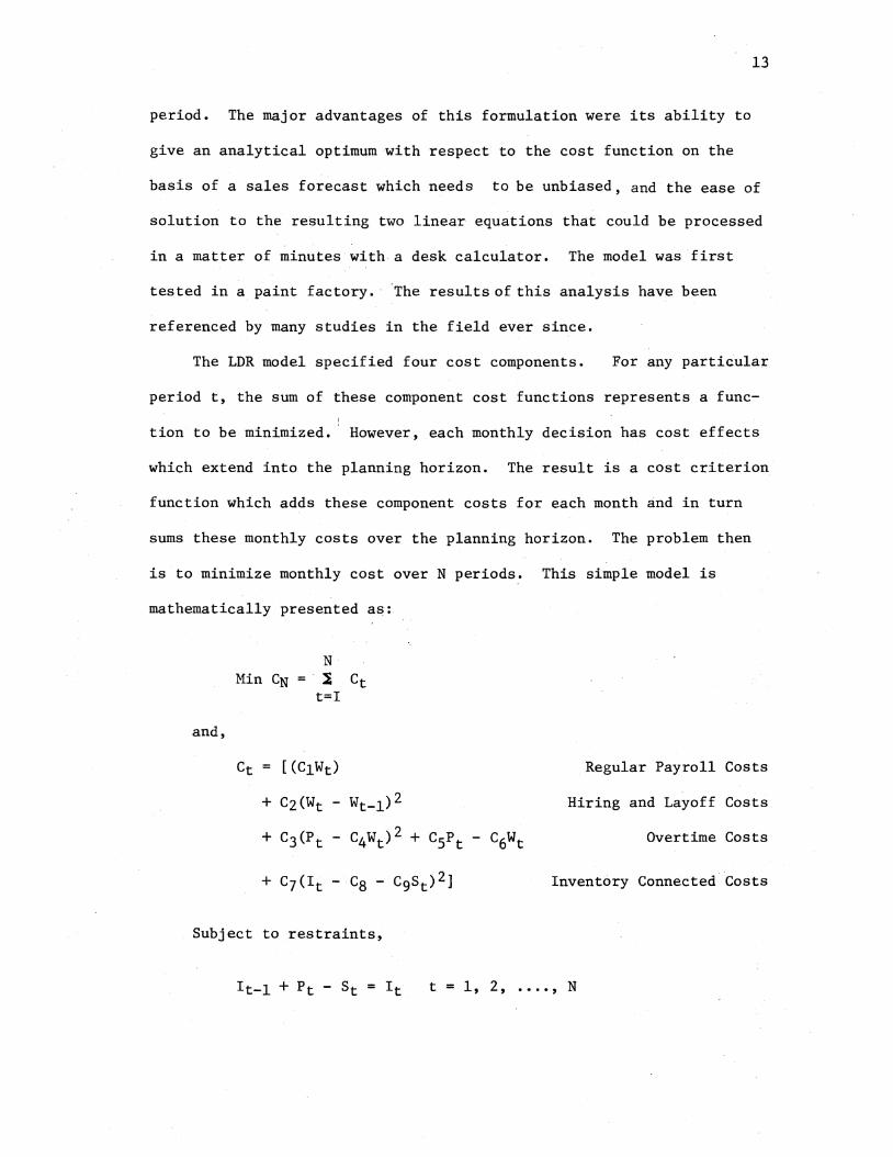
The LDR model specified four cost components. For any particular

period t, the sum of these component cost functions represents a func-

tion to be minimized. However, each monthly decision has cost effects

which extend into the planning horizon. The result is a cost criterion

function which adds these component costs for each month and in turn

sums these monthly costs over the planning horizon. The problem then

is to minimize monthly cost over N periods. This simple model is

mathematically presented as:

and,

N Min CN - l Ct

t=I

Ct = [(ClWt)

+ C2(Wt - Wt-1)2

Regular Payroll Costs

Hiring and Layoff Costs

+ C3(Pt - C4Wt)2 + CsPt - C6Wt Overtime Costs

Inventory Connected Costs

Subject to restraints,

t = 1, 2, •••• , N

14

In the above formulation, Wt, Pt, It and St represent workforce

level, production rate, inventory level, and demand for period t,

respectively. Numerical values for the coefficients c1, ..... Cg, are

statistically estimated from accounting data. C4 is the constant

productivity rate (units of output per man-month)~

Holt, et al., supported their idea of fitting quadratic curves to

the cost function by stating that since the optimality of decision

rules depends on the accuracy with which the mathematical cost function

approximates the true structure of costs, it is desired to know how

close the approximation really needs to be. It turns out that fairly

large errors in estimating and in approximating the cost relations with

quadratic functions lead to small differences in the decisions. Differ-

ences in the decisions lead to even smaller differences in the costs

incurred when the rules are applied. Thus, only reasonable accuracy in

estimating and approximating the cost relationships is sufficient.*

In commenting on the comparison between the LDR and the Hanssmann

and Hess models it is believed that one could just about flip a coin.

In reality the various component cost functions found in practice are

probably neither all linear nor all quadratic, but rather a mixture of

various forms. What is needed is a methodolody which is free of mathe-

matical forms in constructing models for specific company situations.

Heuristic and computer search methods seem to be promising in this

regard .

*Results of the present research and the sensitivity analysis of the LDR cost coefficients f67 ] have made the significance of this state­ment highly questionable!

15

An extension of the LDR model has been developed by Sypkens [63]

which considers plant capacity as a decision variable in addition to the

workforce and production rate. This model is expected to perform best

if it were used with the kind of production systems in which capacity

can be divided into identical units.

In a recent paper Schwarz and Johnson [59] state a hypothesis claiming

that the incremental benefit of aggregate planning (all aggregate

planning models) over the improved inventorymanagementalone may be

quite small. They base their claim on the results of a reported

application of the LDR (the paint factory case). The authors discover

that in this particular case, most of the LDR cost savings have been

due to the reduction in the total inventory costs.*

Gaalman [29] has recently presented an interesting method for

' aggregating on multi-item version of the HMMSmcidel.He has applied the

necessary conditions to reduce the multi-item model to a one item

model. The aggregation technique makes use of the structural properties

of the inventory-production part of the model, and can be performed regardless

of the structure of the workforce-total production part. The author

shows that dissagregation of the optimal decisions of the aggregate

model gives the optimal decisions of the multi-item model.

*The author strongly disagrees with Schwarz and Johnson's claim. The particular cost structure of the selected model is surprisingly biased in favor of this claim; therefore, their stated hypothesis can not be generalized for all cases, and specifically for all aggregate planning models. These authors' discovery of the nature of the LDR cost savings is not original: reference [26], which was published yearsbeforethe publication of the article in question, clearly analyzed the problem (item 3, page 122). However, those conclusions and general­izations were not justified by the author of the latter article!

16

Chang and Jones [18] generalized the LDR model to yield both

aggregate and disaggregate planning in a multiproduct environment and

extended their work to handle the situation in which production cannot

be started and completed in the same period.

Several other s·olution methods that provide optimal results have

been developed and applied with different degrees of success. The

exhaustive enumeration of all feasible solutions is one of these

methods. The approach is practically feasible only when a finite num­

ber of decision variables exist, that is, wh·en the planning horizon is

comparatively short. (See Chapter IV.)

Bellman [ 6 ] has proposed dynamic programming formulations of the

aggregate planning situatio.n which conceptually are interesting. As in

many dynamic programming formulations, what is conceptually interesting

is not often computationally feasible. The major restriction in this

case is the number of possible production states available at each stage

(period). Where a· limited number of production levels are a realistic

assumption, the application of dynamic programming may become feasible.

The advantage of the dynamic programming approach over other optimizing

techniques in this area is that it is independent of cost structure.

Goodman [31] has presented a goal programming approach to solving

nonlinear aggregate planning models. He applies his technique to the

Holt quadratic model and concludes that the effectiveness of such an

approach is highly dependent upon the degree of non-linearity which the

GP model must approximate. The resultssuggest that for relatively low

degree models goal programming may provide an efficient solution

approach, while for higher degree models theapproach may be inappro­

priate.

17

The optimizing procedures for aggregate planning problems with

stochastic demand are currently receiving attention. Kleindorfer and

Kunreuther [41] recently published a paper relating to this case. They

have developed a methodology for showing how forecast horizons for

stochastic planning problems relate to the planning procedures. To

illustrate the approach they have chosen a relatively straight forward

production problem in which the firm can meet a fluctuating demand

pattern through a combination of overtime and inventory-related

options. Their conclusion indicates how this methodology can be

utilized for specifying stochastic horizons for more general aggregate

planning decisions.

Heuristic Decision Rules

The LDR and its extensions continue to provide a harsh standard

for comparing the effectiveness of new approaches to the.problem,

simply because the LDR methods provide known optimum solutions to

specific test situations. The difficulty with mathematical methods is

the requirement that cost functionsbe expressed with either quadratic br

linear relationships, thus limiting the realism which can be incorpor­

ated in the model. The new heuristic methods, as well as computer

search methods to be discussed later, are more free of the constraints of

mathematical forms. Thus, a tradeoff must be made between the desir­

ability of obtaining a known optimum solution to a relatively simplified

model versus obtaining a near optimum solution to a richer, more

realistic model.

Bowman [13] has proposed a new and different approach to many

managerial problems and has used the aggregate planning problem as

18

a sample for study and demonstration of his proposed approach to manag­

erial decision making. His approach establishes the 'form' of decision

rules for aggregate planning through rigorous analysis; however, it

develops the 'coefficients'· for the decision rules through statistical

analisis of management's own past performance (decisions). This is in

constrast to the LDR, in which both the form and the coefficients are

deterxnined by mathematical analysis. Bowman determines the coefficients

by regression analysis on management's past actual decisons. Bowman's

theory is based on the assumption that management is actually sensitive

to the same criteria used in analytical models and that management

behavior tends to be highly variable rather than off center. In terms

of Bowman's theory then, management's performance using the decision

rules can be improved considerably simply by applying the rules more

consistently; since, in terms of the usual dish shaped criterion func­

tion, variability in applying decision rules is much more costly than

being slightly off center from optimum decisions, but consistent in

those decisions.

Gordon [32] developed Management Coefficient models for the Chain

Brewing Company. He also developed an LDR model for the brewery, for

the purpose of comparison. The procedure used simulated the behavior

of the production system under each of the alternate sets of decision

rules by generating production and workforce decisions over a 52-week

period. He concluded that the Management Coefficient Model had a

total cost performance advantage somewhere between the LDR and actual.

However, one serious drawback of the MCM method is the required sub­

jective selection of the form of the rule. It can very easily be

19

selected incorrectly. Obviously, in this case the use of the rule would

lead to less than ideal results.

Vergin [68] argues that in many cases the current state of the

art does not allow the analytical solution of a mathematical model that

is representative of the prototype situation. Therefore, he claims

that the best approach is to model the actual cost functions accurately

in the form of a computer program so that functions more complex than

those allowed in such approaches as linear programming and the LDR can

be included. As in any simulation the approach is to systematically

vary the variables. (e. g., the workforce sizes. and production rates)

until a reasonable (and hopefully near optimal) solution is obtained.

Tests performed by Vergin have shown that substantial benefits may

result from the use of simulation approaches.

Jones [40], in his "Parametric Production Planning," postulates

the existence of two linear feed-back rules: one for the workforce, the

second for the production rate. Each rule contains two parameters. For

a likely sequence of forecasts and sales the rules are applied with a

particular set of the four parameters, thus generating a series of

workforce levels and production rates. The relevant costs are evalu­

ated using the actual cost structure of the firm under consideration.

Using a suitable search technique the best set of parameters is deter­

mined. Again, the results with this simulation approach are quite

encouraging. With Jones' method, there are no limitations in mathe­

matical form of the cost functions; rather they are simply the best

estimates of the cost functions that can be constructed. The selected

parameters are incorporated into the two decision rules to make the

rules specific for a given firm. Thus, while the decision rules are

not optimum in the sense of a mathematically provable optimum, the

procedure introduces aggregate production plans involving cost which

can not be easily improved.

Search Decision Rules

20

One of the most recent approaches to the aggregate planning

problem has been through optimum-seeking computer search methods.

Taubert developed the basic search decision rule methodology in 1967

using the paint company data with the.LDR optimum solutions as test

functions. The results obtained with the paint company data have since

been validated by other authors. Extensions in other environments with

much greater complexity have been developed by Buffa and Taubert [64]

and others. It has been proven that search decision rules can actually

produce realistic decisions in situations so complex that no other

known mathematical programming techniques could be used including

linear, nonlinear, and dynamic programming.

The Search Decision Rule (SDR) approach does not guarantee global

optimality, but it does offer a new way of breaking through the

restrictive barrier imposed by the analytic model, the optimal solution

methods discussed before. The SDR approach proposes building the

most realistic cost or profit model possible and expressing it in the

form of a computer subroutine which has the ability to compute the

cost associated with any given set of decision variable values.

Mathematically, the subroutine defines a multidimensional cost response

surface with a dimensionality determined by the number of decision

variables and the number of the time periods included in the planning

horizon. In short, the cost model forms a multistage decision system

21

model in which each state represents the cost structure of the opera­

tion at the point in time when decisions are made, such as monthly,

quarterly, etc. A computerized search routine is then used to system­

atically search the response surface of the cost model for the point

(combination of decisons) producing the lowest total cost over the plan­

ning horizon. A mathematically optimum solution is not guaranteed,

but the solutions found by the model cannot easily be. improved.

Background of the Improvement Curves

The Improvement Curve is a graphical or analytical representation

of the anticipated reduction in input resources as a production process

is repeated. The reduction in cost or the increase in the rate of

production is achieved in part by the improvement and performance of

direct labor. Other improvements come from management and supporting

staff organizations. The airframe industry was first to use the

predictive value of improvement curves. Empirical evidence supporting

the learning phenomena soon found acceptance in a cross section of

manufacturing industries. Today improvement curves are widely used as an

integral part of production planning and control, as well as a means of

controlling the learning rate of individual operators.

A review of improvement curve applications by Balloff [ 5 ] indicates

that the power function formulation can be used to determine the

productivity increases which accompany the introduction of new products

in a variety of labor intensive assembly situations, including the

manufacture of airframes, electronic and electro-mechanical components,

and machine tools, In addition, the model has also found applicability

22

in instances of both products and process startup in the machine-intensive

manufacture of steel, glass, paper, and electrical products.

The literature so far has concentrated mainly on a somewhat stan­

dardized power function usually referred to as a linear curve. This

formulation was first introduced by Wright l 71] in 1936. Since then, it

has managed to survive in essentially its original form, even though

it has many basic weaknesses. However, a number of alternative functions

have been proposed. Most of these were intended for specific applica­

tions and, therefore, have not affected the popularity of the power

function to any degree. For instance, Cochran [19] proposed an S-type

function which was based on the assumption of a gradual startup. An

S-type function has the shape of a cumulative normal distribution func­

tion for the startup curve and the shape of an operating characteristic

function for the learning curve. Guilbert (French) proposed a compli­

cated multiparameter function with several restrictive assumptions.

More recent works hold somewhat greater promise. Among these,

DeJong [23] proposed a version of the power function which generates

two components, a fixed component which is set equal to the irreducible

portion of the task and a variable component which is subject to learning.

Levy [46] has presented a new type of firm learning function and shows

it to be useful in explaining how firms adapt to new processes and in

isolating the variables that may influence the firm's rate of learning.

Levy's learning function reaches a plateau and does not continue to

decrease or increase as does the power function. Asher [ 3 ] reported on

a variety of different approaches, most of which were proposed during

and immediately following World War II. The main drawback of these

proposed functions is the difficulty associated with parameter estimatio~

23

However, the proposed alternatives have not been able to dislodge the

power function which, apparently, is still the most common one in use

at present time. Pegels [55] offered an alternative exponential func­

tion and demonstrated that it provides a better fit to several sets of

empirical data than the traditional algebraic power function. Bevis

et al. [ 7 ] related the learning curve to an exponential law conunonly

found in physical systems, which characterized the rise time and final

value of output rate.

However, as each proponent of an improvement curve model claims

relative superiority of a particular model over those of earlier

researchers, and as each also gives his examples of specific industrial

situations in which his model performed better, it is reconunended that

any new user of improvement curves make some test runs when selecting

an appropriate model for his own situation. Shultz and Conway [21]

conclude that improvement curves predict a ~irm's progress function

with tolerable amounts of error better than any other device known to

the authors. Thus efforts devoted to determining a proper model and

a proper estimation of parameters will yield a greater return.

Another important consideration in the theory of improvement

curves is the effect of disruption. Disruption constitutes a definite

cost. Hoffman [36], using a displacement of the origin (beginning

cumulative production for a number of repetitions), developed the

improvement curve for a repeat lot and suggested that the amount of

displacement is a function of the amount of learning retained from

previous lots. Cochran [19] presents a comprehensive study of the

effects of various disruptions on the production of long cycl~ products.

24

Carlson, et al. [17] described disruption by a negative delay

function comparable to the delay observed in electrical condensers.

They assumed that an individual's memory is the equivalent of storing

electrical charges in the brain, thus the delay analogy appears reason­

able. Obviously, the rate and amount of delay would depend on "how

much" has been learned or where the task is interrupted in the process

of learning. They showed performance expected as a function of

chronological time or equivalent units. This can also be expressed in

terms of the number of units completed and equivalent units which could

have been completed after an interruption. The amount of forgetting

and the corresponding level of performance is thus showed as a function

of both the performance at the time the process was interrrupted (or

total amount learned) and the length of the interruption. The authors

also showed that if the work performed during the interruption was of

a similar nature, then the rate of forgetting was reduced. Their model

is named the LFL model which represents the Learn-Forget-Learn Phenomena.

Learning curves are applicable to many aspects of production plan­

ning and control today. They can be used to predict the cost per unit

of production, establish selling price, quantity discounts, and forecast

capital needs for budget planning. Learning curves influence delivery

schedules, measurement of shop efficiency, setting of labor standards,

evaluation of employee training programs and improvement of wage incen­

tive schemes. Finally, the learning curve concept can be introduced to

the aggregate production planning area to handle the changing produc­

tivity cases which exist in most real situations.

Since the current research makes use of the somewhat standardized

linear improvement curves, a brief presentation of the analysis of such

curves will follow.

25

Analysis of the Linear Improvement Curves

Empirical studies have demonstrated that incremental improvement in

productivity decreases as the quantity produced increases (Figure l.a).

This relationship is known as an improvement curve. Improvement curves,

when plotted on a log-log graph paper, result in a straight line

(Figure l.b). This straight line is easily expressed by a simple

algebraic equation.

Letting C(n) represent the cost in manhours of a given cumulative

unit n, then the improvement curve can be written as:

C(n) = f.n-b where f = C(l) (2.1)

or as:

log C(n) =log C(l)- b.log n (2.2)

C(l) is the cost of unit one, known as the theoretical base unit cost.

The exponent "b"is a measure of the slope of the linear cost reduction

line.

Equation (2.1) has some important characteristics. Given any two

cost curves Cl(n), c2(n) which have the same value forb, then

where f1 does not equal f2. Now these two expressions can be related

as follows:

C1(n) c2(n)

(2.3)

1.00

0.90

0.80

o. 70

1\ \ ~

r-

90% L.C -.... r--- v -

~ 0.60 \ t---

~ oM

'-' 0.50 -"'i'..

r-

0.40

0.30

0.20

0.10

10

r--

20

r--- lL

30 units

80% L.C

1---- -

40 50 60

a.) Learning Curve Data Plotted on Arithmetic Scale Graph Paper

Ill ~ ::1 0 ..c

1.0

1

......,__ .............

I -·-............ -

I I

90% L. C

r-r- ----"+-.. .......__ r--

SO% L.C

0

units--~

I

-- -I

!'--

,--- -. -~--

00

b.) Learning Curve Data Plotted on Log-Log Scales

Figure 1. Linear Learning Curves

26

27

This result indicates that the ratio of unit costs between the two

curves is a constant (f1/f2), no matter what value n takes. On a

logarithmic scale, a constant ratio means a constant distance between

the two lines on the graph. Hence the two lines must be parallel to

one another; they have the same "slopes."

There are some other characteristics of Equation (2.1) that are

of major importance. Primary among these is the ratio of unit costs for

any two units m and n:

C(m) _ C(l)m-b = [mn]-b C(n) - C(l)n b

Taking M = 2n, the above equation would be written as:

C(2n) = 2-b = S C(n)

(2.4)

(2. 5)

This is conventionally used to define the slope (S) of an improvement

curve. The slope is defined as the ratio of the cost of units in a

doubled quantity relationship. Therefore, a 90% improvement curve

applies in situations where the manufacture of cumulative unit 2n of

output requires only 90% of the manpower that was needed to produce

cumulative unit n.

Given the slope of an improvement curve, one can use Equation (2.5)

to compute the exponent b:

Log S = -b log 2

or,

b = -log S/log 2 (2.6)

28

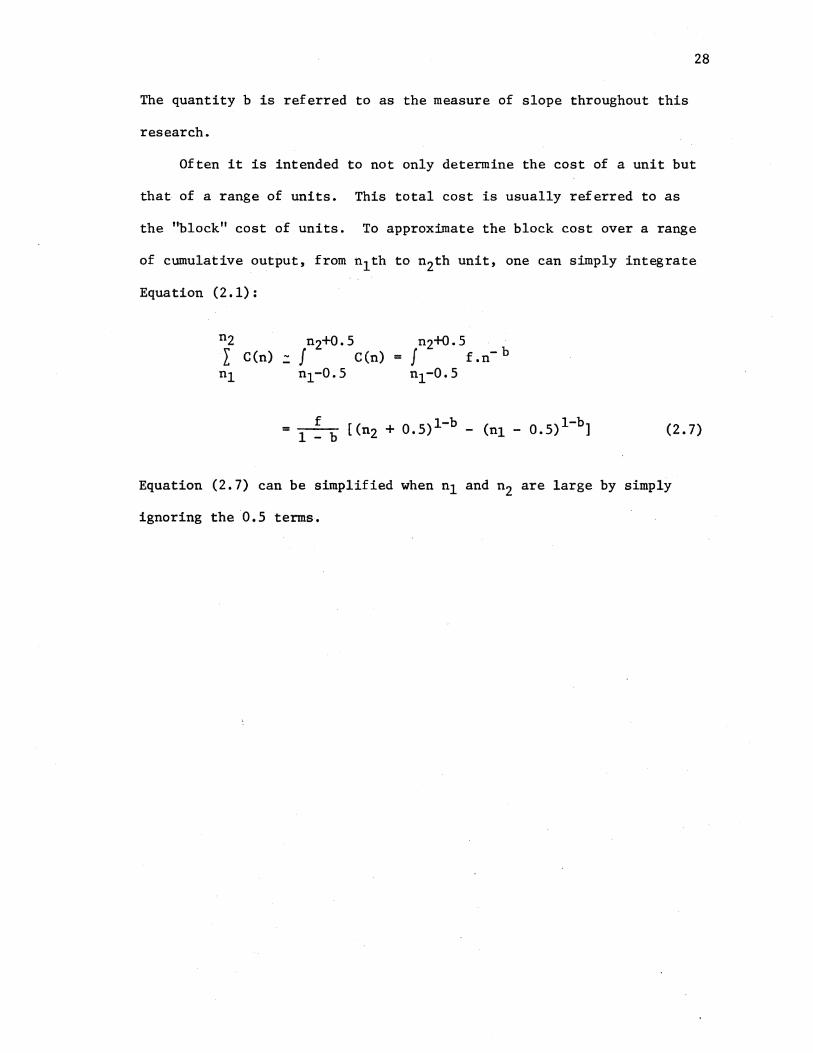
The quantity b is referred to as the measure of slope throughout this

research.

Often it is intended to not only determine the cost of a unit but

that of a range of units. This total cost is usually referred to as

the "block" cost of units. To approximate the block cost over a range

of cumulative output, from n1th to n2th unit, one can simply integrate

Equation (2.1):

n2 n2+0.5 I C(n) - f C(n) n1 nl-0.5

f 1-b 1-b = 1 _ b [(n2 + 0.5) - (nl- 0.5) ] (2. 7)

Equation (2.7) can be simplified when n1 and n2 are large by simply

ignoring the 0.5 terms.

CHAPTER III

AGGREGATE PLANNING MODELS INCORPORATING

PRODUCTIVITY--AN OVERVIEW

Introduction

All aggregate planning models discussed in the previous chapter

utilize a constant productivity factor. In this chapter an overview

of the state of the art in combining aggregate planning models with

changing productivity considerations will be presented.

As mentioned earlier, only two models combining changing productiv­

ity considerations with aggregate planning have been reported in the

literature; however, both have certain limitations and unrealistic

assumptions. A brief explanation of these models and their major

limitations and drawbacks follows.

Orrbeck Model

The first aggregate planning model which incorporated the effect

of worker productivity was developed by Orrbeck et al. in 1968 (53].

This model is an extension of the Hanssmann-Hess model (34] which

presents a linear programming formulation of the aggregate planning­

problem. The cost elements considered in the Hanssmann-Hess model are

regular payroll costs, overtime pay, cost of hiring and firing workers,

and storage and shortage costs. The sum of· these costs accounts for

the total relevant cost in any period. The problem is then one of

29

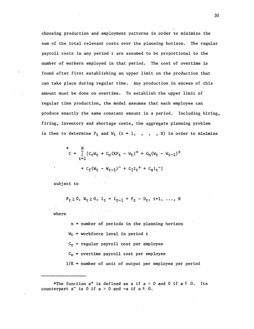
30

choosing production and employment patterns in order to minimize the

sum of the total relevant costs over the planning horizon. The regular

payroll costs in any period t are assumed to be proportional to the

number of workers employed in that period. The cost of overtime is

found after first establishing an upper limit on the production that

can take place during regular time. Any production in excess of this

amount must be done on overtime. To establish the upper limit of

regular time production, the model assumes that each employee can

produce exactly the same constant amount in a period. Including hiring,

firing, inventory and shortage costs, the aggregate planning problem

is then to determine Pt and Wt (t = 1, , N) in order to minimize

* N C I [CrWt + Co(KPt - Wt)+ + Ch(Wt - Wt-1)+

t=l

subject to

where

n number of periods in the planning horizon

Wt workforce level in period t

Cr = regular payroll cost per employee

C0 = overtime payroll cost per employee

1/K = number of unit of output per employee per period

*The function a+ is defined as a if a > 0 and 0 if a~ 0. Its counterpart a- is 0 if a > 0 and -a if a.:> 0.

ch = hiring cost per employee

Cf firing cost per employee

cr inventory cost per period per unit

Cs = shortage cost per unit

It inventory lev~l in period t

By using the proper transformations the problem can be converted into

linear form and be solved by standard linear programming methods.

31

As previously stated the Hanssmann-Hess model assumes a constant

productivity rate for employees. In their extended model, Orrbeck,

etal. drop this assumption and add the assumption that workers are

assumed to have increasing productivity rates. To accomplish this they

assume that all employees fall into one of e experience classes, where

class e represents the most experienced class of workers. Certain.

productivity rates are attributed to certain experience classes.

The essence of the extended model is the assumption that the

number of workers in an experience class will be the number of workers

in the next most experienced class in the preceeding period, minus the

number of workers released from the group. Exceptions are the first

and last groups. The first will consist of newly hired workers, and

the most experienced class will consist of employees in this group in

the previous period plus those promoted into the class by the passage

of time.

Furthermore, this model assumes that the least experienced workers

are fired first, if workers are to be released. Should the number of

workers released in a period exceed the number of employees in the

first class of the previous period, some workers from the second

32

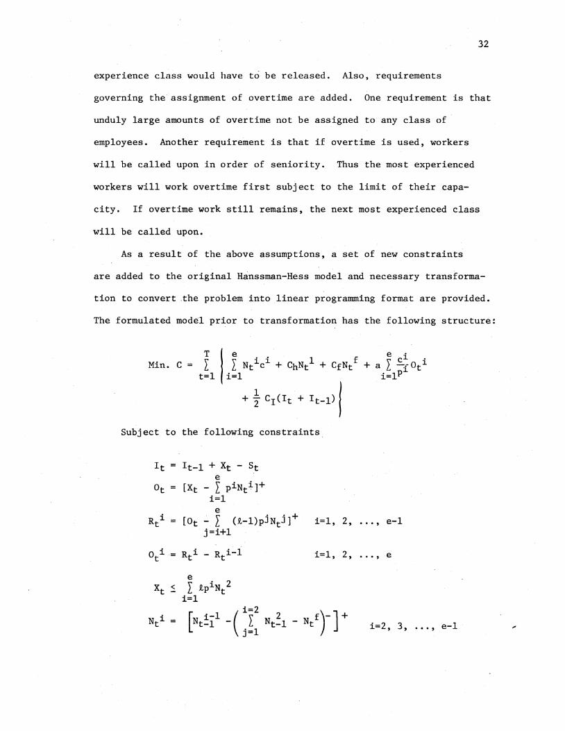
experience class would have to be released. Also, requirements

governing the assignment of overtime are added. One requirement is that

unduly large amounts of overtime not be assigned to any class of

employees. Another requirement is that if overtime is used, workers

will be called upon in order of seniority. Thus the most experienced

workers will work overtime first subject to the limit of their capa-

city. If overtime work still remains, the next most experienced class

will be called upon.

As a result of the above assumptions, a set of new constraints

are added to the original Hanssman-Hess model and necessary transforma-

tion to convert .the problem into linear programming format are provided.

The formulated model prior to transformation has the following structure:

Min. C T e f ~ ci . I I Ntici + ChNtl + CfNt + a l .. -{ OtJ.

t=l i=l i=lp

+ t Cr(It + It-lll

Subject to the following constraints

It = It-1 + Xt - St e

Ot = [Xt - I piNti ]+ i=l

e R i [Ot I

. . + i=l, 2, e-1 t - (9,-l)pJNtJ] ... '

j=i+l

0 i t Rti - Rti-1 i=l, 2, ... ' e

i=2, 3, ... , e-1

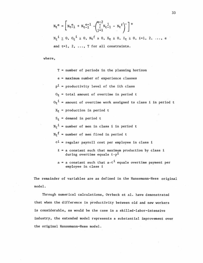
33

[ (e-2 .

e e-1 J Nt~l + Nt-1 - .L Nt-1 J=l

and t=l, 2, •.. , T for all constraints.

where,

T = number of periods in the planning horizon

e = maximum number of experience classes

pi productivity level of the ith class

Ot total amount of overtime in period t

Oti amount of overtime work assigned to class i in period t

Xt production in period t

st = demand in period t

Nti = number of men in class i in period t

Ntf = number of men fired in period t

ci = regular payroll cost per employee in class i

£ = a constant such that maximum production by class i during overtime equals £•pi

a = a constant such that a.ci equals overtime payment per employee in class i

The remainder of variables are as defined in the Hanssmanri-Hess original

model.

Through numerical calculations, Orrbeck et al. have demonstrated

that when the difference in productivity between old and new workers

is considerable, as would be the case in a skilled-labor-intensive

industry, the extended model represents a substantial improvement over

the original Hanssmann-Hess model.

34

Although the above model considers a variety of relevant assump­

tions, it has two major drawbacks. First, this model assumes that the

productivity rate of each experience class is related to the time span

during which the experience classes are involved in the firm's activ­

ities. That is, the productivity rates are only related to the passage

of time. However, as mentioned earlier, empirical studies demonstrate

that an increase in productivity can be systematically related to the

cumulative output of the firm. This cumulative output is not

necessarily directly proportional to elasped time. Orrbeck et al!s

assumption could be relevant if employees are utilized only on regular

time. In such a case the output per employee could be assumed pro­

portional to the number of production periods. In reality, however,

utilization of overtime and undertime is frequently experienced by the

firms. Due to these alternative ways of workforce utilization, groups

of employees starting at identical productivity levels may have differ­

ent productivity rates after one or more production periods. The lack

of proper consideration of this phenomenon may be the major drawback

of the Orrbeck et a!.' s model.

A second drawback of this model is its computational limitation

in the majority of empirical situations. This limitation is due to the

large number of variables and constraints encountered in the linear

program formulation. For example, for a 12 month period (usually con­

sidered in aggregate plans) and 6 experience classes (higher numbers

may be assumed by most firms), 288 variables (excluding slack and

artificial variables) and 168 constraints will be required in the

model (after necessary transformations). Therefore, this model seems

to be computationally unattractive.

35

As will be seen later, the assumptions regarding experience classes

considered by Orrbeck et al are too unrealistic to be considered for

the firms producing long cycle products. Some of these·assumptions

are only relevant for the case of short cycle products. Furthermore,

the effects of progress and retrogression, which will be explained

later, are not incorporated in the Orrbeck et almodel.

Ebert Model

The second and the most recent model which merges productivity

considerations and aggregate planning was developed by Ebert in 1976

[25]. The advantage of this model over the earlier one is due to the

direct use of the learning curve analysis in aggregate planning.

Ebert's model can also be applied using more complex cost functions.

The cost structure for production planning in each time period (t)

used by Ebert to illustrate his proposed method is:

where

N

L Tc t=l t

Tct = ClWt Direct Labor

2 + Cz(Pt- C4tWt)/C4t + C3[(Pt - C4tWt)/C4tJ Overtime

+ cswt + c6clwt

+ C7(Wt - Wt-l) if Wt > Wt-l

+ c8 (Wt-l - Wt) if Wt > Wt-l

Variable Labor Overhead

Hiring or

Firing

36

+ C9(It +Itx) if It > Itx

+ Clo(It - Itx) if It < Itx

Inventory Carrying or

Inventory Stortage

where Wt = director workforce size, Pt = production quanitity, It =

ending inventory, c4t z average production per worker (same as 1/K ·

in Orrbeck, et al. model), and Itx =desired ending inventory.

Evidently, other forms of cost functions could have been used to

demonstrate this model. Ebert does not assume a constant value for

C4, rather he assumes that it changes as a function of the cumulative

output of the manufacturing facility. The learning curve is usually

expressed in terms of man-month per unit output, the inverseof C4.

For proposed levels of output across several future time periods,

cumulative output will increase and average productivity will vary from

period to period. The expected productivity for each of these time

periods can be obtained from the manufacturing progress function

(learning curve) and subsequently used as C4.

To determine the expected productivity for a range of proposed

output in a future time period, the general form of manufacturing

progress function considered by Ebert is:

(3.1)

where Yi = man-month required to produce the ith cumulative unit

of output, K m man-months required to produce the first unit of

output (initial productivity). b • the absolute value of slope of

the progress function and i varies continuously.

37

The average productivity over a range of cumulative output (from

Ath to Bth units) proposed for a future month is obtained by first

integrating (3.1) to obtain (3.2).

B f (i) = f Krbdi

A K[B(l.O-b) _ A(l.O-b)]/(1.0-b)

Then (3.2) is divided by B-A, thus,

YA,B = K[B(l.O-b) - A(l.O-b)]/[(1.0-b)(B-A)]

The value of C4 is then given by c4 = 1.0/YA,B. Thus, the cost of

(3.2)

(3.3)

any proposed production plan can be approximated, once the parameters

in (3.3) are specified.

A search routine is utilized to determine the solution to the

above model. This search model consists of three major sub-components:

a main program, an evaluation routine, and an exploratory subroutine.

The manufacturing progress function is incorporated in the evaluation

routine. For any proposed change in Pt (made by the main program or

by the exploratory subroutine), the productivity factor C4 in the

objective function of the evlauation routine changes on the manufacturing

progress function. The expected productivitiy (C4) for the modified

range of cumulative production output is used to evaluate the cost

for each new plan. The main program in this model makes major changes

in the decision vector values based on favorable change indicated by

the exploratory routine. The exploratory routine modifies the existing

decision vectors by small increments.

38

Ebert shows the potential significance of his model by generating

a series of aggregate plans for various learning rates. These plans

are then proposed to be used to develop manpower schedules, for cashflow

analysis, and for making product pricing decisions.

The Ebert's model has one major drawback: the model does not

incorporate the effect "learning" properly, and under rare situations

it can only take into account the effect of "progress" on the produc­

tivity. The term "improvement" is usually applied to the general

relationship between unit cost reduction and the cumulative number of

units produced. The term "learning" is applied strictly to that portion

of cost reduction which occurs without major method or design changes,

and the term "progress" to the effect of those changes.

To notice the limitations of this model, one can consider the

case of short cycle products, for example, in which different experience

classes with different productivity rates can be recognized. A close

look at Ebert's model in this case highlights the fact that the model

treats every member of the workforce level in every period as if he

were hired at the beginning of the first period. The productivity rate

of a new worker is assumed to be the same as the productivity rate of

the most experienced one. This is due to the fact that in this model

the basis for determination of the productivity rate of a given employee

in a given period is the cumulative product units produced by the

workforces, without consideration to when an employee was hired.

This model could be almost valid only in a situation where the

workforce level at every period of the planning horizon comprises only

those employees (or a proportion of those) who have been hired at the

beginning of the first period. That is, where the workforce level is

monotonically non-increasing. This situation, of course, is not very

likely to occur, since the decision rules in aggregate planning

usually indicate fluctuating levels of workforce for the purpose of

coping with the fluctuating demand throughout the planning horizon.

Furthermore, even under this rare situation, and for the case of

production of long cycle products where a crew of men is usually

assigned on a job, the reduction in the size of workforce generates

significant disruption in the improvement pattern of productivity.

This disruption is not incorporated in Ebert's model.

39

To illustrate the impact of the above point, an extreme case where

the workforce level is monotonically increasing could be imagined.

Figure 2 portrays such a case for a six month planning horizon. Nbtice

that the workforce in each period is comprised of different classes of

employees with different experience levels. The rectangulars in each

column represent these classes. The rectangulars with lower numbers

represent the classes of employees with higher experience levels and

therefore with higher productivity rates.

In the above case the model would assume similar productivity

rates for all classes of employees in each period. For example, in

the 6th period all lower five classes are treated the same as the

upper class which has the highest productivity; the productivity rate·

of the most experienced class (rectangular No. 1) is applied even for

the newest class of employees (rectangular No. 6). However, it is

evident that the workforce level in period No.6 is comprised of 6 classes

of employees with different experience levels and productivity rates.

The above discussion concludes that Ebert's model is not a true

representation of the production system in situations where the total

1

1 2

1 2 3

1 2 3 4

1 2 3 4 5

1 2 3 4 5 6

1 2 3 4 5 6

production periods

Figure 2. Experience Classes in a Monotonically Increasing Workforce Level Situation

40

41

productivity improvement pattern is not solely due to the progress

effect (almost all situations with the exception of highly automated

processes). The search routine developed by Ebert to obtain solutions

to his model is the one developed by Hooke and Jeeves [38]. Since

development of this routine, a number of other routines have been

developed which are more efficient in handling complex functions which

may even be subject to a set of constraints. Application of such

routines should have a greater advantage since aggregate decisions are

usually subject to constraints such as: limited storage space, limited

assignment of overtime, limitations on the rate of hiring and firing

manpower, and other restrictions. These-constraints and the considera­

tion of the production as function of workforce skills incorporated

in an aggregate planning model could enhance the applicability of the

model and reduce implementation and operational problems.

Considering the importance of precise determination of the

productivity factor in the cost function of the aggregate planning

problem, the insufficiencies of the models discussed in this chapter

seem to be critical.

More reliable models based on more realistic assumptions for both

cases of long cycle and short cycle products have been developed in

this research. They will be presented in Chapter V and VI, respectively,

following the discussion of the general solution approach.

CHAPTER IV

SOLUTION METHODOLOGY

Introduction

The two models developed in this research utilize the same solu­

tion methodology. Since the structures of these models are oriented

toward the concepts of the applied solution methodology and these

concepts are frequently referred to during the course of model descrip­

tion, it is appropriate to present a detailed description of the

selected solution methodology prior to the presentation of the models.

The purpose of this research is to introduce more realism into

mathematical models of aggregate planning. As a general rule, small

incremental improvements in model realism require exponential increase

in the mathematical complexity, and the more complicated and realistic

the model, the more critical the problem of choosing a promising solu­

tion technique. Therefore, selection of an appropriate solution tech­

nique is of special importang.e for the current research.

There are numerous optimization techniques that can be used to

solve mathematical models. Some are strictly analytical in nature:

differential calculus, Lagrangian multipliers, linear progrannning and

dynamic programming. Others are quasi-analytical, such as the gradient

following techniques, and still others are strictly heuristic in nature.

Both the quasi-analytical and heuristic techniques offer the 4ser the

hope of finding a global optimum, but not the guarantee of finding one.

42

43

At this time no single optimization technique can be used to solve

all mathematical models. This means that optimization is still an art

involving a careful match between technique and model. This match must

be made skillfully, with constant concern for the basic fact that a

solution to a model can be no better than the model itself. Consequently,

the model builder faces the dilemma that the more complicated he makes

the model, the lower the probability of finding the global optimum. In

the past this problem was so serious that the model builder had to

restrict himself to simple models that could be solved by analytic

techniques. Today the computer has made possible many new-quasi­

analytical and heuristic search techniques. These techniques have

increased significantly the probability of finding the global optimum of

a complex model and have placed before the model builder a very powerful

set of mathematical tools.

The incorporation of dynamic productiviy consideration into the

aggregate planning problem, as will be seen later, introduces a con­

siderable amount of complexity which almost eleminates the possibility

of utilizing an analytic solution technique for these models. For

example, the dynamic nature of the cost functions assumed by these

models resultsin heterogeneous decision systems (systems with stage

dependent structures) that necessitate the utilization of heuristic

solution techniques. Although these techniques do not guarantee the

global optimum, better overall results are achieved by developing

highly realistic models that are near optimum in preference to the

globally optimum models that are unrealistic. After all, it is the

real-world situation we wish to optimize rather than a model.

44

Because of the above fundamental reasons, the Search Decision Rule

is the solution methodology chosen for the models developed in this

research. A detailed description of this methodology follows.

The Search Decision Rule (SDR) Methodology

The heart of the SDR approach lies in a synthesis of computer

optimization methods and multistage decision theory. In essence the

approach proposes building the most realistic cost model possible and

expressing it in the form of a computer subroutine which has the ability

to compute the cost associated with any given set of values for decision

variables. Mathematically, the subroutine defines a multidimensional

cost response surface with a dimensionality determined by the number of

decision variables and the number of time periods included in the plan­

ning horizon. In short, the cost model forms a multistage decision

system model where each stage represents the cost structure of the

operation at the point in time when decisions are made, such as monthly,

quarterly, etc. A computerized search routine is then used to system­

atically search the response surface of the cost model for the point

(combination of decisions) producing the lowest total cost over the

planning horizon. A mathematical~y optimum solution is not guaranteed,

but the method finds solutions which can not be easily improved.

Multistage Model Development

The basic building block of the SDR approach is the one stage

decision model. This model represents the cost structure of the firm

at some particular point in time when decisions are to be made. Thisis

usually monthly. The one stage models are then joined together to

45

form a multistage model which represents the operation of the firm over

the planning horizon. Figure 3 portrays the one-stage model construe-

tion process and identifies the state and decision vector inputs, the

stage returns and the state vector output.

Actual Projected Operations

at Time t = 1

r

1 so

Stage 1 Computational

ut Algorithm

te Inp Sta

Vee tor PI Dl

Parameter Vector

Decision Vector

Figure 3 • One Stage Decision Model

Sf

Outp ut;: te or

Sta Vect

The terms illustrated in Fig~re 3 and used in the SDR approach are

defined as:

Stage: Any real or abstract entity in which transformation takes place. In the context of the operations planning problem, a stage represents the point in time when decisions are made concerning the operation of the system. At each stage a decision (D) creates a return (r) and places the system in a new state (S).

Input State Vecotr S : A j component vector S = (Sm, So2' ••• , So,t) which transmits information to stage 1 and serves to describe the state of the system at the beginning of the stage 1 trans­formation.

Output State Vector S1: A j component vector S1 = (Sll, S12, ••• , Slj) which transmits information to stage 2 and serves to describe the state of the system at the end of the stage 1 transformation. The transition. function is given by S1 = Tl(S~ D1, PI)•

Parameter Vector P1: Ani component vector P1= (Pll' Pl2' ••• Pli) containing those factors that affect r1 and s1 and·must be specified to define the problem.

46

Decision Vector D1: A k component vector D1 = (d11, dlz, ••• d1k) which controls the operation of stage 1, given ~ and P1.

Stage Return r1: a single decision

A scalar used to measure the utility of the stage as valued function of the input state, parameter and vector r1 = f1(~, D1, P1),

A one stage decision system model is constructed for each month in

the N month planning horizon and then the models are joined together to

form a serial mutlistage decision system. A serial mutlistage system

is termed homogeneous if the individual stages are identical, and termed

heterogeneous if they are not. A heterogenous system is produced when

the coefficients of the cost function change from one stage to the

other. The models developed in this research are of heterogeneous type,

because the productivity rates are assumed to be changing from one

period to another. The structure of the cost function in these models

is dynamic in nature.

A simple multistage system is illustrated in Figure 4 • The

operations planning model in its simplest form consists of optimizing

the total expected N stage return of the multistage model shown in

this figure. This optimization is performed over the decision vectors

(Dl, Dz, ••• , DN), given the values specified by the initial system

state vector~' and subject to possible constraints on both .the

decision and state variables. The decision made at each stage should

be optimal with respect to the entire N stage system rather than optimal

with respect to a particular stage.

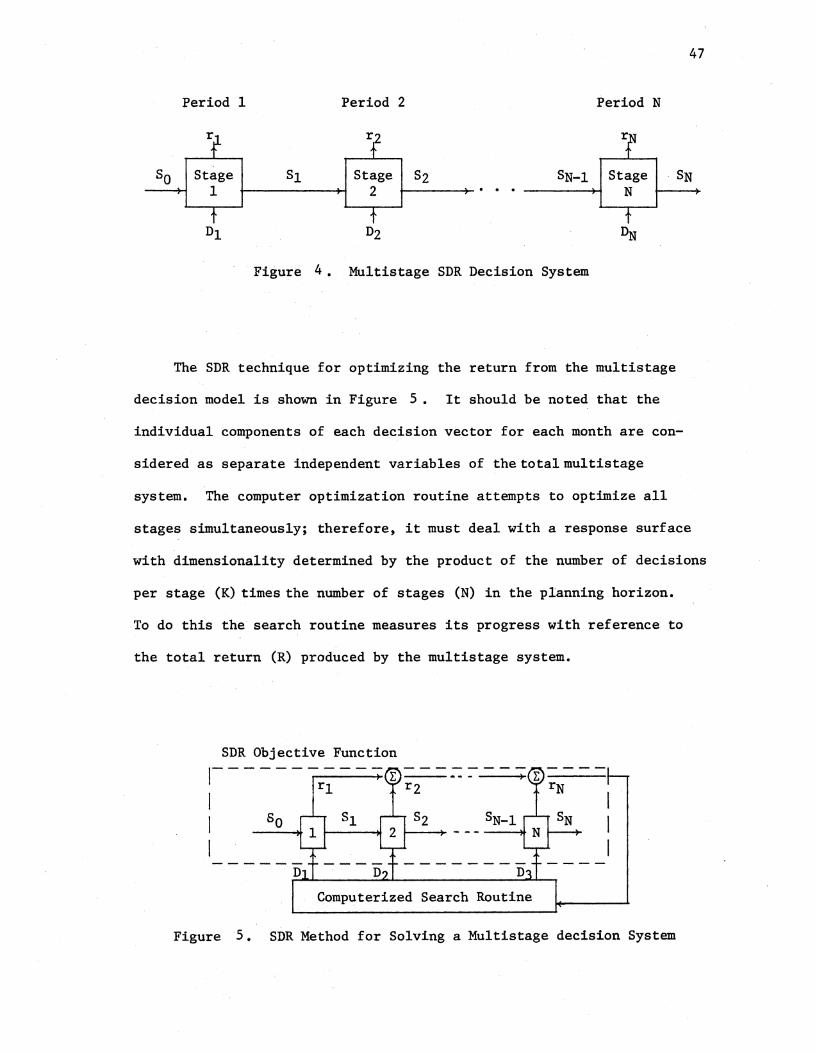
47

Period 1 Period 2 Period N

r r r

so Stage sl Stage s2 SN-1 Stage SN 1 2 N

Dl D2 ~

Figure 4 • Multistage SDR Decision System

The SDR technique for optimizing the return from the multistage

decision model is shown in Figure 5 • It should be noted that the

individual components of each decision vector for each month are con-

sidered as separate independent variables of the total multistage

system. The computer optimization routine attempts to optimize all

stages simultaneously; therefore, it must deal with a response surface

with dimensionality determined by the product of the number of decisions

per stage (K) times the number of stages (N) in the planning horizon.

To do this the search routine measures its progress with reference to

the total return (R) produced by the multistage system.

SDR Objective Function

~------ lr~- --, }: I I so s2 sN-1

I

Computerized Search Routine

Figure 5. SDR Method for Solving a Multistage decision System

48

The computer search solution to the SDR model provides decisions

for each month of the N month planning horizon. Normally, one is

interested only in implementing the month 1 decisions contained in

vector D1. Decision vectors D2, D3, ••• , DN provide a planning purpose

forecast of possible actions, but they are based on a successively

shorter planning horizon. Therefore, when it is time to make decisions

for the next month, the model is updated with a new sales forecast,

initial conditions, etc., and optimized again.

The total return (R) need not be additive as shown in Figure 5 •

It might consist of a weighted sum, such as present value discounting

techniques; or it might consist of a complex formulation based on utility

concepts. The SDR approach provides great flexibility in this respect.

The information flow in a typical SDR monthly cycle is shown in

Figure 6. Following the month 1 optimization of the model by the

search routine, the decisions contained in Dl are reviewed and imple­

mented by management. The projected decisions for the remaining

months in the planning horizon (D2, D3, ••• , DN) are used to form the

SDR starting vector for the month 2 search (performed at the beginning

of the second month). In this way the search routine does not have to

start all over again from a randomly selected starting point in N­

dimensional space. Use of the SDR computed starting vector sharply

reduces the search time and trereby reduces the cost of computing the

decisions for month 2 and all subsequent decisions.

SDR Programming System

The complete SDR programming system for homogeneous models con­

sists of a main program and two subroutines containing the search

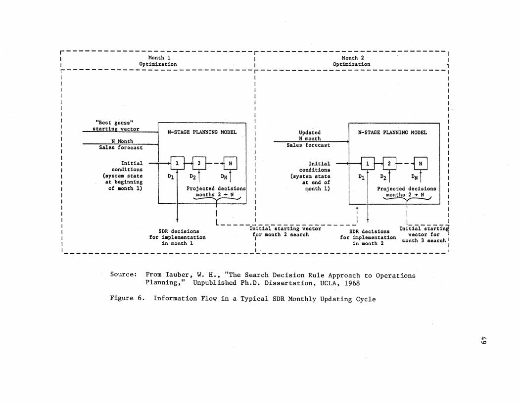
r------------------------------r----------------------~-------1 1 Month 1 1 Month 2 1 1 Optimization 1 Optimization 1 r------------------------------r------------------------------1

"Best guess" startin vector

N MC>nth Sales forecast

Initial conditions

(system state at beginning of month 1)

I I I I I I I I I I I I· I I I I I I

N-STAGE PLANNING MODEL 1 Updated N-STAGE PLANNING MODEL 1 1 N month 1 1 Sales forecast 1

. I I

I ~ I J Initial - N 1 1 conditions 1 1 (system state DN 1 1 at end of 1

Projected decisions 1 ~onth 1) Projected decisions 1 months 2 + N 1 months 2 + N 1

SDR decisions for implementation

in month l

I I I t I

I I I

L---- -r~it'ii'l-sta;ting ;ector----- _I In~tiaCst'artin~ for month 2 search SDR decisions vector for I 1 for implementation month 3 search 1 1 in month 2 1 I . --------------------------------------------------------------

Source: From Tauber, W. H., "The Search Decision Rule Approach to Operations Planning," Unpublished Ph.D. Dissertation, UCLA, 1968

Figure 6. Information Flow in a Typical SDR Monthly Updating Cycle

50

routine and the cost model. The operating sequence of the system is

shown in Figure 7 • The main program initializes all variables and

reads in the sales forecasts, the starting decision vectors, the

initial state vector and all model parameters. The main program then

calls the search routine which systematically explores the response

surface of the cost model until either the limit on the number of cost

function evaluations is reached or a better point cannot be found.

MAIN PROGRAM

• Read in input information

• Initialize

. Print results

SEARCH ROUTINE

. Determine move strategy

COST MODEL

. Compute cost of given decision

Figure 7 • SDR Progrannning System

51

The search routine continuously varies the decision vector components

in an attempt to minimize the total cost of operation over the entire

planning horizon. At the conclusion of the search, control is returned

to the main program for printing out the final decision vector and

other information relating to the operation of the cost model. Typical

computer times for a complete SDR search ranges from three seconds to

two minutes on most medium-size computers, depending upon the complexity

of the cost model and the number of dimensions.

For heterogeneous models, the program should be supported by a

subroutine which systematically constructs the cost model at each stage.

As will be seen later, such routines are developed in this research

to properly re-structure the cost model at every stage with respect to

the levels of state and decision vectors in the preceeding stages.

Since these routines include a considerable number of computations and

are called for every proposed change in the level of decision vectors,

the computer time required for the search process is relatively higher

for these models.

SDR Advantages and Disadvantages

The advantages and disadvantages of using the SDR approach as

opposed to the traditional analytic model (optimal solution approach)

are summerized below:

SDR Advantages

1. Permits realistic modeling free from restrictive assumptions, such as closed form mathematical expressions, linear/quadratic cost functions, etc.

52

2. Permits a variation in mathematical structure from stage to stage (heterogeneous stages) so that anticipated system changes, such as productivity improvement, wage increases, etc., can be considered.

3. Provides the operating manager with a set of current and pro­jected decisions.

4. Permits optimizeddisaggregate decision making.

5. Lends itself to evolutionary cost model development and pro­vides solutions at desired points in the iterative process.

6. Facilitates sensitivity analysis and provides sensitivity data while the search routine is converging on a solution.

7. Easily handles cash flow discounting, nonlinear utility func­tions, multiple objectives, and complex constraints.

8. Offers the potential of solving many otherwise impossible operations planning problems.

SDR Disadvantages

1. Optimization using computer search routines is an art and it is currently impossible to state which search routine will give the best performance on a particular objective function.

2. Decisions made by this methodology may not represent the absolute global optimum.

3. Responsesurfacedimensionality appears to limit the efficiency.

Search Routine Operation

The heart of the SDR approach is the computerized search routine.

A large number of search routines have been developed during the re-

centyearsand vary in design from traditional gradiant approaches to

rather heuristic programs. Regardless of the particular design, all

search routines may be classified by the way they answer two questions.

Assuming that the routine has selected a particular point on the

response surface by specifying the decision vector, then the two key

questions are:

53

1. What is the next direction of movement?

2. How far should the movement be in the given direction?

The direction of movement may be along the gradient, along the

deflected gradient, along each of the coordinate axis, or in a randomly

selected direction. Once the direction has been determined; one step,

several steps, or a one-dimensional line search may be made. In quanti­

tative terms, the questions are answered by the following iterative

equation:

where Di is an n-dimensional decision vector with components (dl, d2,

••• , dn) representing the trial point for the ith trial or iteration,

Ai is a positive constant, and Pi is an n-dimensional direction vector

evaluated at the ith iteration. The vector Pi answers the first ques­

tion by specifying the direction to be taken in moving away from point

Di and the magnitude of AiPi answers the second question by specifying

a step is to be taken in that direction.

Figure 8 is a flow chart illustrating the major elements of a

comprehensive search routine. The routine starts by selecting the

initial starting vector for the search (box 1).

Boxes 2, 3, 4, 5 and 7 constitute what is frequently called the

search code, or search algorithem. Collectively, they determine the

location of the next point, evaluate the response surface at that point,

determine the best direction of movement, and at the same time, monitor

the progress to see if any action need by taken to speed up convergence.

Box 6 contains appropriate logic to check if the search code has

moved the search outside of the feasible region; if so, it computes

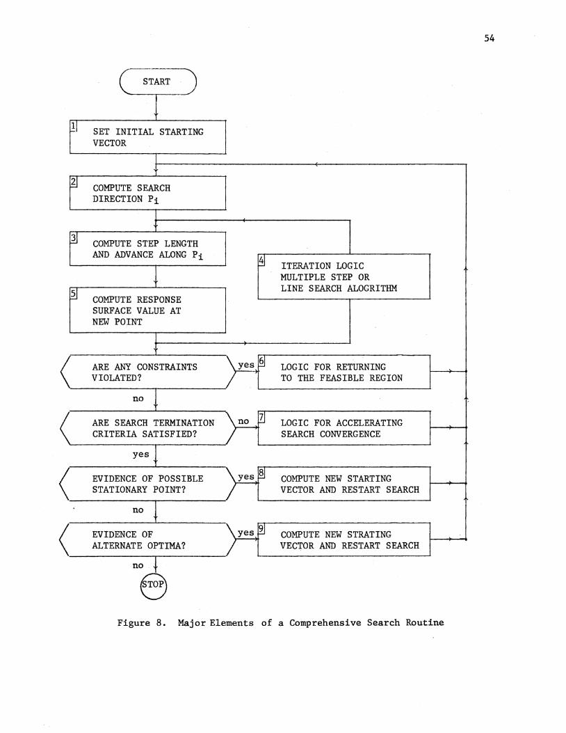
54

c-·-----~-~ START ·

~ 11 SET INITIAL STARTING

VECTOR

I t

.?J COMPUTE SEARCH DIRECTION Pi

I f

11 COMPUTE STEP LENGTH AND ADVANCE ALONG Pi

~

+

ITERATION LOGIC MULTIPLE STEP OR

~ LINE SEARCH ALOGRITHM

COMPUTE RESPONSE SURFACE VALUE AT NEW POINT

I t

ARE ANY CONSTRAINTS F §] LOGIC FOR RETURNING VIOLATED? TO THE FEASIBLE REGION

no I ARE SEARCH TERMINATION ~

?J LOGIC FOR ACCELERATING CRITERIA SATISFIED? SEARCH CONVERGENCE

yes {

< EVIDENCE OF POSSIBLE F ~ COMPUTE NEW STARTING STATIONARY POINT? VECTOR AND RESTART SEARCH

no I <

EVIDENCE OF F ~ COMPUTE NEW STRATING ALTERNATE OPTIMA? VECTOR AND RESTART SEARCH

no t e

Figure 8. Major Elements of a Comprehensive Search Routine

55

the necessary step size and direction to bring the search back. There

are a large number of sophisticated techniques available for use, but

most require the solution of bounding problems that are almost as compli­

cated as the objective function itself. As a result, many users prefer

to transform the problem to one without constraints. This transforma­

tion is done by adding penalty functions to the original objective

function and then optimizing the model as if it were unconstrained.

Box 8 represents the logic used to determine if the routine has

become stuck on a relatively flat portion of the response surface.

Typical tests for this condition include either random or symetric spot

checks at various trial points in the neighborhood of the suspected

stationary point. If no improvement is noted, the routine moves to the

final test for alternate optima. If a better point is found, the search

is restarted using the location of the new point as the starting vector.

Box 9 conducts a test for the alternative optima by restarting the

search from different locations on the response surface. If they all

converge to the same point, there is increased probability that the

global optimum has been found.

Selection of a Search Code

A considerable number of search routines have been developed

during the last two decades which utilize different search codes. As

it was stated earlier, it is currently impossible to make a priori

prediction concerning the performance of a search code on a particular

response surface. Often no amount of argument can ever determine before

hand if a particular method will work more efficiently then another, or

even work at all. The performance of a search code depends on the

56

particular type of system to be optimized and how well the program it­

self has been written.

Taubert [65] has conducted a comprehensive experiment to test the

performance of four promising search codes applied to the SDR methodology.

These codes are: conjugate gradient [28], variable metric [22,27], pat­

tern [38,69] and simplex [11,51].

Conjugate gradient and variable metric codes consider the responsP.

surfsce in terms of a quadratic Taylor's series approximation model and

base their move strategy on this representation. If the response sur­

face is quadratic, the routines are guaranteed to locate the optimum

point on an n-dimensional response surface in n-steps, assuming rounding

errors are not significant. If the response surface is not quadratic,

the routines use a local quadratic approximation of the surface to gener­

ate promising search directions. The resulting procedure is then itera­

tive rather then n-step with the rate of convergence determined by the

routines' response to the local quadratic approximation from one itera­

tion to the next.

The conjugate gradient search code uses the method of conjugate

gradients as the main vehicle for solving the quadratic series model of

the response surface. The solution is used to produce new search

direction vectors.

The variable metric code approaches the problem by approximating

the matrix of second derivatives, or Hessian matrix, using information

about the way in which the first derivatives vary from one iteration to

another. Both conjugate gradient and variable metric methods require

the.numerical computation of first partial derivatives.

57

The pattern and simplex search codes are striclty heuristic in

nature and do not view the response surface in terms of a specific

analytic model. Consequently, they do no require the numerical estima­

tion of derivatives. In a series of performance tests on a 60-dimen­

sional SDR model, Taubert concluded that the pattern search code per­

formed better than the other codes. Faster convergence was the basic

criterion for this comparison.

In the course of his work, Taubert developed a new code which is

essentially a modified version of the pattern search code. The new

code is termed the adaptive pattern search. The modification was made

to the code developed by Weisman, Wood and Rivlin [69]. This code

features a system for independently controlling the step size of each

variable as well as some rather sophisticated search termination logic.

These features considerably enhance search efficiency and performance

over the original Hooke and Jeeves version.

The operation of the Weisman et al. version of the pattern search

code was carefully studied by Taubert in connection with the performance

tests on a SDR model. Taubert found that the performance of the pat­

tern search code could be improved by a factor of two, and sometimes

more, by systematically changing the pattern growth multiplier. The

multiplier is used to control the length of the pattern move as defined

by the equation:

T(I) = P(I) + G·[C(I)- P(I)]

T is the new temporary base point computed by the pattern move equation,

P is the old base point prior to the present pattern move and explora­

tory search sequence, C is the search location at the end of the

58

exploratory search, G is a constant called the pattern growth multiplier

and (I) represents the ith component of each vector. It can be seen

that increasing the value of G causes the search to make larger pattern

moves, while smaller values reduce the distance covered by the move.

Weisman et al. used a fixed value of G = 2.0 in their code, thereby,

permitting a simplification of the general equation to:

T(I) = 2C(I) - P(I)

The pattern move is basically an acceleration device to move the search

rapidly along relativley straight ridges in n-dimensional space.

Consequently, it is hypothesized that if the value of G could be varied

based on the progress made by the search code, then it might help the

acceleration move adapt to the local terrain and thereby improve the

overall efficiency of the search code. Inotherwords, the multiplier

would be varied if the search appeared to be slowing down or stuck at

some point.

The adaptive control logic is designed around a measurement of the

rate of convergance made by the search as it moves towardtheminimum.

If the rate is high, no change in G is made; if it is low, a small

change is made; and, if it is very low, a large change is made. Deter­

mination of what is a high, low and very low rate depends on the parti­

cular response surface under study. The values used in this work are

based on empirically determined values from investigations performed

on the multistage SDR test models. A FORTRAN listing of the complete

adaptive pattern search code with documentation, and the glossary of

the variables in this program are included in the Appendix.

Application of SDR to the Aggregate

Planning Problem

59

Since the current research utilizes the original HMMS cost struc­

ture as the basis for analysis of the research results, it is appropri­

ate to demonstrate the application of the SDR methodologytooptimization

of this particular cost model. The HMMS model application using the

quadratic paint factory cost function is probably the most widely

studied in the aggregate planning field. This model has achieved the

status of the standard of comparison for other aggregate planning

techniques. Most of the challenging techniques have been unable to

equal the LDR's performance of the paint factory model.

Figure 9 summarizes the four basic cost equations that makeup

the paint factory cost model. In this model, the regular payroll

cost for a period is a linear function of the workforce level in that

period.

The hiring and layoff costs are not associated with the size of

the workforce, but rather with changes in its size. This relationship

is approximated by a quadratic function.

The overtime cost function is not based on the size of the work­

force or on the production rate, but rather on the production rate

given the workforce. The overtime rate may be 50% of regular pay for

week days and 100% of regular pay for weekends. Hence a quadratic

approximation is assumed to be more accurate than a linear approxima­

tion. It should be noticed that any idle time incurred is included in

the direct payroll cost function in this model. The factor 5.67 in

the overtime cost function is the average productivity factor (units

DIRECT PAYROLL COST

Direct Workforce (wt)

OVERTIME COST

Production Rate Pt, Gallons/Month

HIRING/LAYOFF COST

Workers Laid off

(Wt - Wt-1)

Workers Hired

C2 = 64.3(Wt - Wt-1) 2

INVENTORY CARRYING/ STOCK OUT COST

Net Inventory It, Gallons

C4 = 0.0825(It - 320) 2

Source: From Holt, C. C., Modigliani, F., Muth, J. F., and Simon, H. A., Planning Production, Inventories and Workforce, Prentice-Hall, 1960.

Figure 9. Cost Relationships of the Paint Factory Cost Model

60

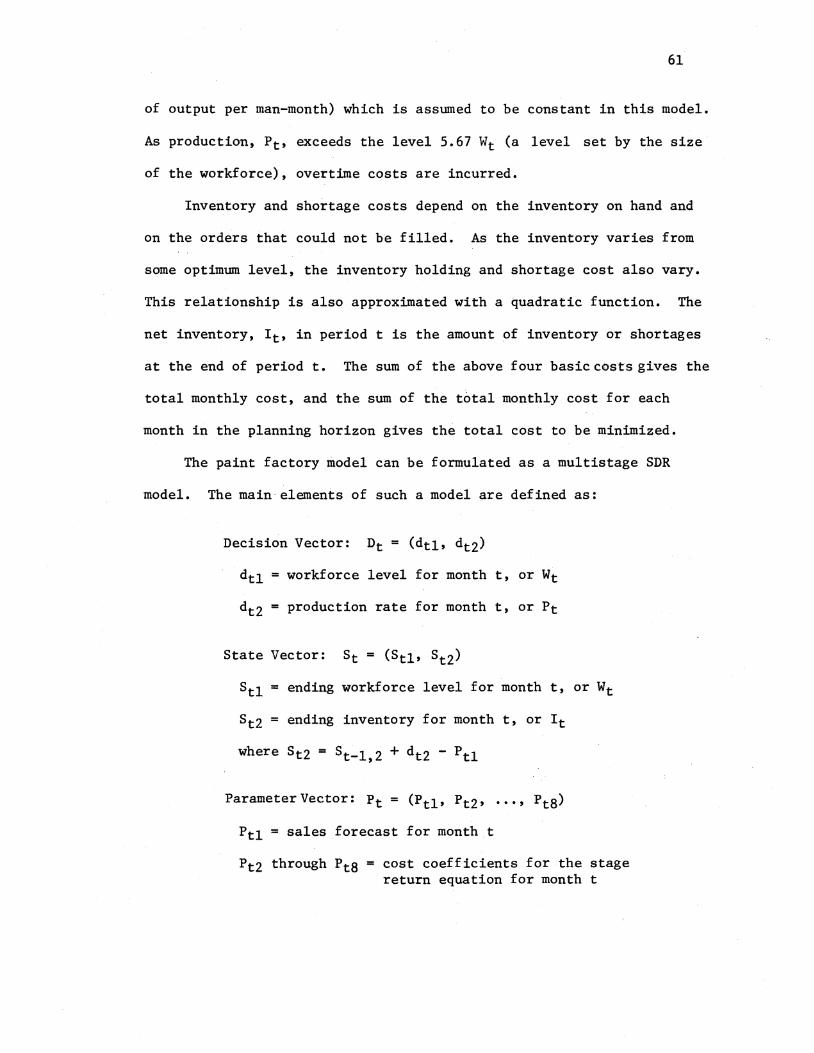
61

of output per man-month) which is assumed to be constant in this model.

As production, Pt, exceeds the level 5.67 Wt (a level set by the size

of the workforce), overtime costs are incurred.

Inventory and shortage costs depend on the inventory on hand and

on the orders that could not be filled. As the inventory varies from

some optimum level, the inventory holding and shortage cost also vary.

This relationship is also approximated with a quadratic function. The

net inventory, It, in period t is the amount of inventory or shortages

at the end of period t. The sum of the above four basic costs gives the

total monthly cost, and the sum of the total monthly cost for each

month in the planning horizon gives the total cost to be minimized.

The paint factory model can be formulated as a multistage SDR

model. The main elements of such a model are defined as:

Decision Vector: Dt = (dtl• dtz)

dtl workforce level for month t, or Wt

dtz = production rate for month t, or Pt

Stl = ending workforce level for month t, or Wt

Stz = ending inventory for month t, or It

ParameterVector: Pt = (Ptl• Pt2• ••• , Pts)

Ptl = sales forecast for month t

Ptz through Pt8 = cost coefficients for the stage return equation for month t

62

rt = Pt2dtl + Pt3Cdtl - St-1,1)2 + Pt4(dt2 - Pt5dti) 2

+ Ptsdt2 ~ Pt6dtl + Pt7<8t-1,2 + dt2 - Ptl - Pta) 2

Total Return:

N R L rt

t=l

Since the cost structure of the paint factory model does not

change with time, the stage return equation would have a simplified

form, including the constant parameters:

rt = 340 dtl (Regular Payroll)

2 + 64.3 (dtl - St-1,1) (Hiring and Firing)

2 + 0. 2 (dt2 - 5. 6 7 du) + 51.2 dt2- 281 dtl (Overtime)

2 + .0825 (St-1,2 + dt2 - Ptl - 320) (Inventory)

It can be seen from the composition of the decision vector

Dt = (dtl, dtz) that each month included in the forecast horizon

requires the addition of one complete stage, or two additional indepen-

dent variables (dimensions) to the multistage model. One variable is

for the workforce level and the other is for the production rate.

Therefore, an N period planning horizon would require an optimization

of a 20-dimensional function.

Assuming an initial inventory level of 263 units and initial

workforce level of 81 men, the SDR solution to the paint factory model

for a 10 month planning horizon is demonstrated in Table II.

The results generated by the SDR show that this methodology has

the ability to virtually duplicate the results of the mathematically

(

63

TABLE II

RESULTS OF OPTIMIZATION OF THE PAINT FACTORY COST MODEL

A. DECISIONS AND PROJECTIONS

Month Demand Work Production Inventory

Average Force Productivity

1 430 77.7 470.5 303.5 5.67 2 447 74.3 444.1 300.6 5.67 3 440 70.9 417.1 277.7 5.67 4 316 67.7 381.7 343.4 5.67 5 397 65.1 376.2 322.5 5.67 6 375 62.7 363.8 311.4 5.67 7 292 60.7 348.9 368.3 5.67 8 458 59.0 359.4 269.7 5.67 9 400 57.4 329.3 199.0 5.67

10 350 56.1 272.2 121.2 5.67

B. COST ANALYSIS OF DECISIONS AND PROJECTIONS ($)

Mo. Payroll Hiring & Overtime Inventory Total Firing

·I 26,406.07 . 715.19 2,447.78 22.45 29,591.40 2 25,247.18 747.03 1,978.09 31.04 28.003.34 3 24,105.72 724.73 1,476.17 147.88 26,454.50 4 23,029.24 644.56 511.47 45.05 24,230.33 5 22,122.18 457.64 986.83 0.53 23,567.18 6 21,327.44 351.32 1,015.87 6.13 22,700.76 7 20,639.67 263.11 810.97 192.46 21,906.21 8 20,068.63 181.38 1,936.16 208.91 22,395.08 9 19,509.80 173.70 740.77 1,207.64 21,631.91

10 19,080.42 102.55 -1,408.60 3,259.04 21,033.41

241,514.22

64

optimum rule (LDR). The total costs indicated by the SDR deviate within

0.1% from the ones generated by the LDR.

Once again, it should be noticed that the structure of the paint

factory cost model is static. By means of the SDR approach it is

possible to eleminate this restriction, as will be seen in the later

chapters.

The aggregate decisions are usually subject to a variety of con­

straints: ending inventories are limited to some predetermined

amount; assigned overtime is limited by the size of workforce; the

nprmal workforce size is limited; there are limitations on the rate

of hiring and firing new employees; etc.

The SDR methodology can incorporate the above constraints into the

cost model and thereby generate solutions with less operational and

implementation difficulties. The cost models optimized by SDR are

not restricted to linear and quadratic forms; therefore, more realistic

and general cost models can be developed and optimized using this

methodology. The efficiency of the SDR methodology is highly depend­

ent upon the type of the search code utilized. As mentioned before,

the pattern search code has demonstrated the best performance in this

regard.

Figure 10 shows the results of a typical test run in conjuntion

with performances of three search codes, namely conjugate gradient,

variable metric and the pattern search, as have been used for optimi­

zation of the paint factory model. It should be noted that in every

case pattern search exhibits the fastest convergence.

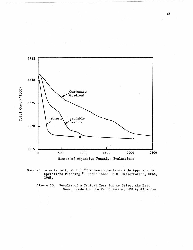
,.... 0 0 0 ...... <r.r ..._,

.j.,l

Cll 0 u ...... t1l .j.,l

0 H

2335

2230

2225

2220

2215 0 500 1000 1500 2000 2500

Number of Objective Function Evaluations

Source: From Taubert, W. H.~ "The Search Decision Rule Approach to Operations Planning," Unpublished Ph.D. Dissertation, UCLA, 1968.

Figure 10. Results of a Typical Test Run to Select the Best Search Code for the Paint Factory SDR Application

65

CHAPTER V

MODEL I. LONG CYCLE PRODUCTS

Introduction

This research distinguishes between the long cycle products and the

short cycle products. The output rate of firms producing long cycle

products cannot be directly related to the productivity rates of the

individual workers, as is the case for short cycle products. Long cycle

operations are inherently a team activity. Long cycle work is long cycle

because it is complex and requires a large amount of manpower. Therefore,

it must be broken down into separate tasks in order to permit enough

labor effort to be expended to meet schedules. In many areas -this

requires establishment of teams of men on the shop floor, each performing

his specific task on the same basic unit. The unit cost (timewise)

usually requires operating at low unit quantities of inventory, so that

when a man or group falters, the effect on those around is felt quickly.

The need to coordinate their efforts closely ties the workers together

as a team.

There are several consequences of this team relationship. For

example, the pace of each work center tends to be limited by the slower

members. At the same time, those members may work better than they

might have alone. In such a case, the improvements found by one

member may help the others. The rhythm of the production process is

66

67

generally more difficult for a long cycle work center to acquire.

This may have some real effects on the pattern of cost reduction.

The constant flow of minor method changes also upsets this rhythm to

a greater degree. This prevents the operation from gaining the full

benefit of those changes.

The changes in the manpower level can also impose significant

changes on the unit cost of long cycle products. Aggregate production

plans usually indicate a fluctuating workforce level schedule for the

purpose of optimally coping with the fluctuating demand levels. The

purpose of this chapter is to perform a study of the disruption effect on the

productivity improvement pattern as a result of manpower level changes

as these changes relate to the aggregate production planning problem.

Analysis of the Disruption Effect of Manpower Changes

As stated in the previous section, the unit cost of the long cycle

productcannotbe directly attributed to the productivity rates of

individual workers. That is, the productivity rates of different

workers or groups of workers cannot be separately considered and

treated. This is due to the nature of team activities. In such

activities, whenever an increase or decrease occurs in the level of

the workforce, theproductivity of the whole team is usually affected.

As an example, the effect of a simple manpower increase could be con-

sidered. Some possible results of this change are:

Some tasks are continued by those already performing them.

Some tasks are assigned to new men who have no experience in performeing them.

Some tasks are reassigned from men already performing them to the new men. Presumably the supervisor establishes the

new distribution of tasks with reference to individual capabilities.

Some tasks are removed from men already performing them and reassigned to others of the original team (men with some'experience) to secure better balance of tasks or other advantages.

It is conceivable that a major crew expansion could result in

68

such a reshuffling of tasks that everyone receives a new reassignment.

This would of course have a serious effect on productivity and is thus

usually avoided.

Estimating the cost effect of manpower changes in long cycle

manufacturing is of special importance because of the substantial

cost premiums generated by the constant addition of untrained people

and loss of trained ones. This not only reflects personnel turnover,

but also the unique needs of long cycle manufacturing to meet produc-

tion acceleration demands, implement frequent process improvement, and

adjust manpower to match the relentless reduction of unit costs and

the corresponding rise in the rate of output.

The method of estimating the effect of design change can be used

as the basis for quantifying the effect of manpower changes on pro-

ductivity. This is a reasonable approach because manpower changes have

characteristics very similar to those of design changes. In both cases

the work is new to the operator, the penalty of the change is larger

for events occuring further in the production sequence, and it shrinks

rapidly as production continues. This is true because, for instance,

at the early stages of production, in which the employees are unexper-

ienced and have low productivites, introduction of design change or

addition of new (unexperienced) manpower do not introduce significant

drops (disruptions) in the overall productivity level. In the later

69

stages of production, the result is opposite.

Since new work is not added by a manpower change, it could be

expected to resemble a task "turnover" most closely. By definition,

when a task is deleted of the same size--timewise--as that which is

added, the change is called a task turnover. However, a manpower change

is less severe than a design change since supervision, tooling, support

personnel, and other crew members are left unaltered.

Measuring the cost effect of manpower changes requires four steps:

1. Define the type of change which will be covered;

2. Measure the effect of each type of change on crew assignments to develop an "index of new manpower;"

3. Translate the index into an equivalent task turnover ratio;

4. Use the ratio and the methods based on the study of the cost effect of design changes to estimate the cost of the manpower changes.

In order to conduct the above analysis it is first necessary to

analyze the cost effect of design changes and then interpret the

concept of the task turnover in terms of manpower changes. Consequently,

the following section is devoted to the analysis of the cost effect of

design changes.

Cost Effect of Design Changes

Cost reduction arising from design changes is better described

as "progress" rather than as "learning." However, such changes can

increase as well as reduce unit time costs, and often generate irregular

and confusing cost patterns.

Any change generates a substantial initial labor cost penalty

even if the ultimate effect is cost reduction, termed "progress."

i

70

This fact is logically interpreted as a "learning" phenomenon, since

change introduces new work into a work center performing an existing

task. U The learning curve analysis provides a method of estimating the

cost effect of task changes.

Of the many possible applications of learning curve cost analysis,

long cycle products have the greatest need for this application since

learning continues throughout the life of a product. The use of learning

curve methods to predict changes in cost is based on the linear

learning curve. The discussion here will therefore focus on the com-

\ putation of change costs for linear curves.

Figure 11 illustrates a typical change on a long cycle product,

occuring at unit 20. The high penalty paid on the first few units fol-

lowing the change with a rapid recovery of the original base cost level

is illustrated in this figure. Such a cost pattern will naturally

cause a temporary slow-down in the rate of output, unless extra men

are assigned. The logic of this situatuion is quite conceivable, but

it first requires the definition of what is meant by "a change " which

involves the following elements:

1. The original task being performed by the work center. This is designated by C0 (n) - The original log linear curve.

2. The portion Cr(n) which is removed from the original task C0 (n).

3. The portion Cc(n) which continues to be performed after the change is incorporated. But since this equals the difference between the original task and that removed, this portion can also be written as Cc(n) = C0 (n) - Cr(n)

4. The new task Cs(n) which replaces the deleted portion Cr(n) of the original task. Normally it will continue at the same slope as before.

5. The revised total task after the changes have been made, is designated by C1(n) = Cc(n) + Cs(n).

J­z :::> ....... U) a:: :::> 0 I

1000.-----~----~--------~----~-------

ORIGINAL TASK Cn(n)

REVISED TASK C1 (.n)

. CONTINUED TASK Cc(n)

200~----~----~--------L-----~------~ 10 20 50 100 1000

UNITS PRODUCED

Source: From Cochran, E. B., Planning Production Costs Using the Improvement Curve, Chandler Publishing Co., 1968.

Figure 11. Unit Time Cost Effect of a Typical Change for Long Cycle Product

71

72

In order to demonstrate the application of the above definitions

to a typical case the following situation can be considered: Consider

an 85 percent slope for an original task C0 (n), such that the unit

cost of unit 500 is 300 hours (C0 (500) = 300). The base cost can be

found using the basic log linear curve formula:

or,

thus

-b C(n) = f·n

b = -log(.85)/log(2) = .2344

f 0 = (300)(500)(" 2344 ) = 1,287 hours

Now suppose that of this task some 10 percent is deleted after

unit 20. This makes the continued task 90 percent of the original

one, or:

Cc(500) = (.9)(300) = 270 hours

and the theoretical base unit cost for this task is:

fc = (270)(500)(· 2344 ) = 1,158 hours

For simiplicity, let us take the new task Cs(t) to be exactly the

same size as the task removed Cr(n). This will also permit the

measurement of the cost of making a change when the final task Cl(n)

is the same size as the original task·c0 (n). This will illustrate

a significant cost penalty in such a case.

Being the same type of work as C0 (n), the new task will also be

on an 85 percent slope with a base unit cost equal to 10 percent of

the original task (the size of the new task is 10 percent of the

73

original one). Therefore, fs = 128.7 hours.

Now the unit cost calculations for the revised task as the result

of this disruption can be performed using the above data. Since the

change was made after completion of unit 20, the first unit of the

revised design is unit 21. The cost of this unit originally would

have been:

C0 (21) = 1,287·(21)(-. 2344) = 630 hours.

The revised cost Cl(21) can be found by using definition (5)

above. This cost can be computed in two steps, corresponding to the

two elements of the revised task itself:

1. The first element, C~(21), represents the continued portion of the task which continues to be performed. This equals:

Cc(21) = fc·(21)(-. 2344) = (1,158)(.490) = 567 hours

2. The second element, Cs(21), represents the new portion of the task, and equals:

Cs(21) = fs·(l)-" 2344 = (128.7)(1)(-. 2344) 129 hours

Therefore, the combined cost will be:

Cl(21) = Cc(21) + Cs(21) = 567 + 129 = 696 hours

and this value compares with the original level as follows:

Cl(21) - C0 (21) = 696- 630 = 66 hours (10.5 percent)

The 66 hours difference is approximately 10.5 percent of the original

level.

The subtantial cost premium of 10.5 percent is noticed, even

though a task was added of the same size as that removed.

Similarly, the cost of a subsequent unit--say, unit 30~can

be computed with some interesting further conclusions:

(1,287)(30)<-· 2344 ) = 580

Cc(30) = (1,158)(30)(-· 2344) = 522

Cs(30) (129)(30-20)<-· 2344 ) 75

Cl(30) = 531 + 75 = 597

The unit cost difference between the revised task and the original

task is Cl(30) - C0 (30) = 17 hours. This indicates a cost premium

of only 3 percent.

The cost premium drops from 66 hours to 17 hours when only ten

additional units are produced. The more units produced after a

change, the closer is the revised cost level to the original one;

and finally, after some number of units, the disruption effect will

damp and the revised curve will approach the original curve. As

Figure 11 indicates, a sharp slope immediately after the disruption

occurs. It helps to understand this if one recalls that the slope of

the learning curve plotted on the log/log scale reflects the ratio

of cost reduction between succeeding units.

Tabulation of the costs which contribute to the revised curve in

this example shows exactly how the gradually reducing slope occurs:

N

21 22 23

Co(n)

630 623 617

Cc(n)

567 561 555

C8 (n)

129 llO

99

CJ(n)

696 671 654

74

75

For the basic cost line C0 (n), the cost for unit 22 drops only

7 hours or 1 percent below that for unit 21. But for the new cost line

C1(n), there is a reduction of 25 hours or almost 4 percent. This

large change creates the sharper slope shown in Figure 11. Such a

change occurs because of the large reduction in the new portion of

Cl(n), namely Cs(n). The drop from unit 21 to unit 22 amounts to

19 hours, or 15 percent, because those costs represent only the first

and second units of the new work produced. It should be noticed that

Cc(n), the continued portion, has the same ratio of cost reduction

(slope) as does C0 (n) itself. Going from unit 22 to 23, C0 (n) drops

6 hours and 1 percent while C1(n) drops 17 hours and 3 percent. The

reason is the same, but now the cost of the new work Cs(n) drops less

rapidly so that cl(n) does also. The slope of C1(n) is therefore not

so sharp between units 22 and 23 as between 21 and 22. And so the

leveling trend continues as more units are produced.

Since this example assumes that a task is deleted of the same

size as that which is added (10 percent of the original task), the

change is called a "task turnover" of 10 percent. Usually a design

change involves adding a task of different size than that deleted.

Consequently, when the difference is larger there can be a substantial

shift in the entire level of the curve. However, this latter case is

not of major concern of this research, since the cost effect of the

manpower change, which at this point is the subject of the research

concern, generally corresponds to the task turnover.

General Formula For Unit and Block Change Costs

Further definitions can simplify the formulation of the change

costs. Let us define:

n0 The unit produced before changing the task.

r = The ratio which the task removed bears to the basic cost curve, orr= Cr(n)/C0 (n).

s = The ratio which the new task bears to the basic cost curve, or s = Cs(n)/C0 (n-n0 ).

76

It should be noted thatCs(n), the new task, must be related to C0 (n-n0 )

rather than C0 (n) because each value reflects n0 fewer performances of

the task. Therefore, Cs(n) = sC0 (n-n0 ).

Now since Cl(n) = Cc(n) + Cs(n), and Cs(n)

or

and with minor rearrangements:

It should be noted that except for C0 (n), the original cost

curve, all other cost functions have been eleminated. Hence all cal-

culations can be made-using this curve. In the event of a "task turn-

voer," r and s are equal in the above expression. Therefore, in this

case the formula becomes:

C1(n) = (l-r)C0 (n) + rC0 (n-n0 )

The unit cost difference, the difference between the revised task and

the original task for the nth unit is:

UCD(n) = C1(n) - C0 (n) = (l-r)C0 (n) + sC0 (n-n0 ) - C0 (n)

or,

UDR(n) -b

= (n-n£) s (n) -b - r

-b = s (1-E.Q.)

n

77

- r

This equation indicates that as n becomes larger, n0 /n becomes smaller;

a steady decline occurs in the UDR as more units are produced after a

change. Eventually, the value of UDR approaches s - r. This means

that a difference between r and s eventually creates a corresponding

permanent shift up or down in the cost level. However, in the event of

task turnover, this difference is zero meaning, that the two curves will

eventually merge to a unique one (the original curve).

The block (cumulative cost for a range of units) change cost

formula can be written on the basis of the same analysis. Using the

same symbols and terms as before, the block cost may be expressed as

the sum of two separate tasks, namely the one continued after the

change is made and the new task. The simplest way to express this

mathematically is to sum the costs of all units produced for the block

in question. Therefore, for all units produced from unit n1(n1 ~ n0 )

and through n2 the formula will be:

[(l-r)C0 (n) + sC0 (n-n0 )]

or

n2 n2 (1-r) I C0 (n) + s I C0 (n-n0 )

or

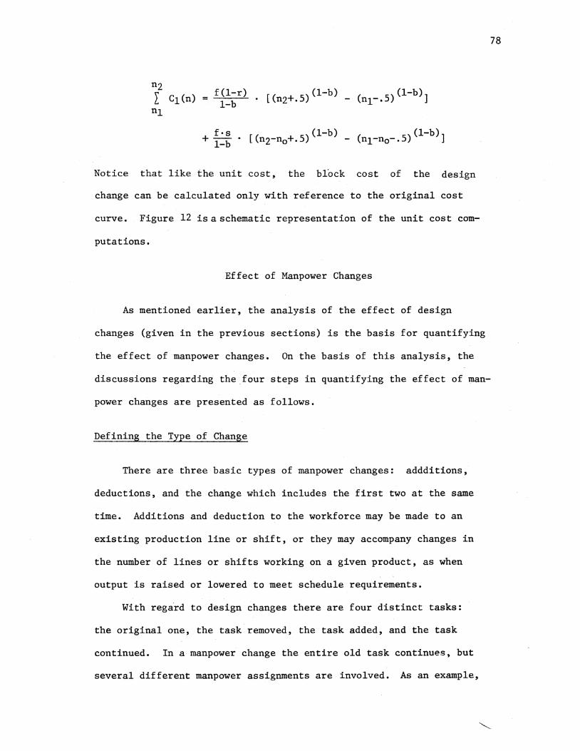
f(l-r) . [(nz+. 5)(1-b) _ (n1-. 5)(1-b)] 1-b

f·s (1-b) (1-b) + l-b · [(n2-n0 +.5) - (nl-n0 -.5) ]

Notice that like the unit cost, the block cost of the design

change can be calculated only with reference to the original cost

curve. Figure 12 isaschematic representation of the unit cost com-

putations.

Effect of Manpower Changes

As mentioned earlier, the analysis of the effect of design

changes (given in the previous sections) is the basis for quantifying

the effect of manpower changes. On the basis of this analysis, the

discussions regarding the four steps in quantifying the effect of man-

power changes are presented as follows.

Defining the Type of Change

There are three basic types of manpower changes: addditions,

deductions, and the change which includes the first two at the same

time. Additions and deduction to the workforce may be made to an

existing production line or shift, or they may accompany changes in

the number of lines or shifts working on a given product, as when

output is raised or lowered to meet schedule requirements.

With regard to design changes there are four distinct tasks:

the original one, the task removed, the task added, and the task

continued. In a manpower change the entire old task continues, but

several different manpower assignments are involved. As an example,

78

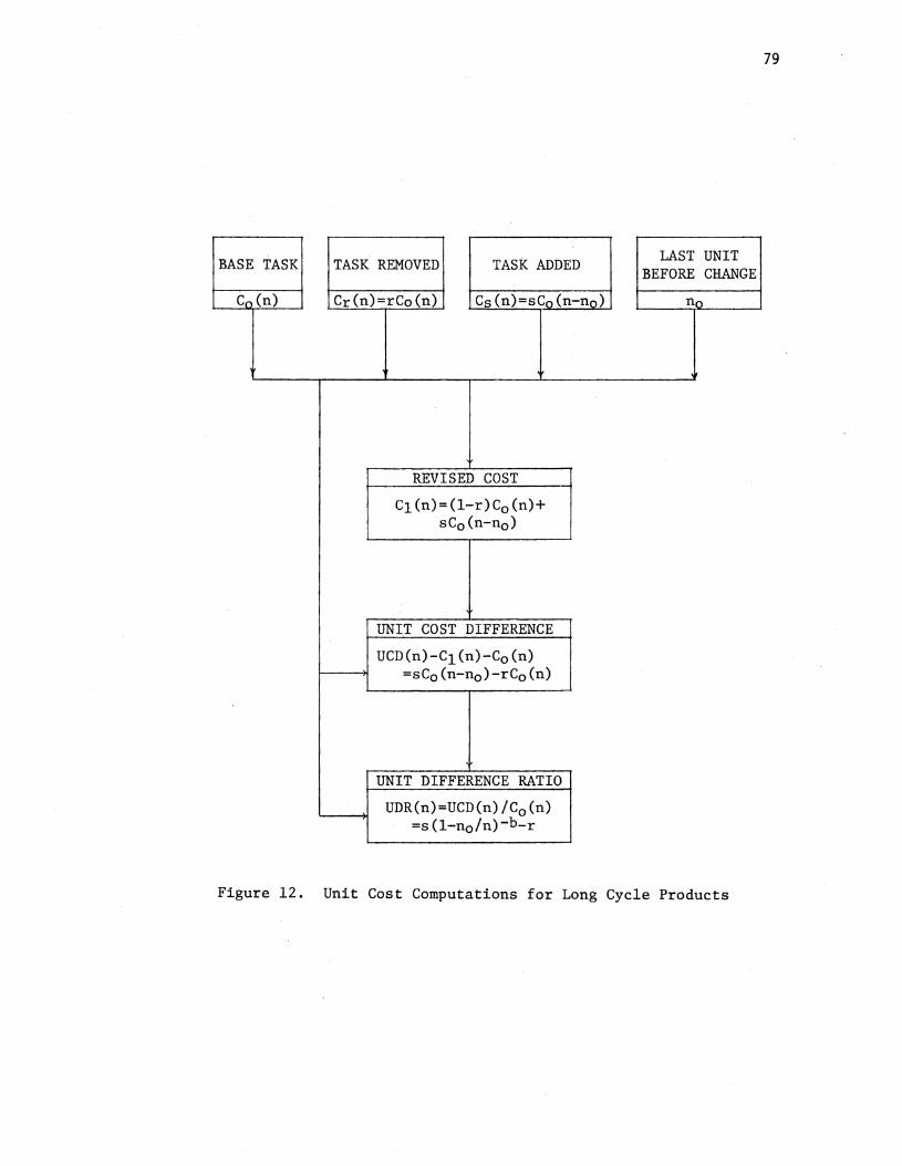
79

BASE TASK TASK REMOVED TASK ADDED LAST UNIT BEFORE CHANGE

C,.. (n) Cr(n)=rCo(n) Cs(n)=sCo(n-no) no

REVISED COST

Cl(n)=(l-r)C0 (n)+ sC0 (n-n0 )

UNIT COST DIFFERENCE

UCD(n)-Cl(n)-C0 (n) =sC0 (n-n0 )-rC0 (n)

UNIT DIFFERENCE RATIO

UDR(n)=UCD(n)/C0 (n) =s(l-n0 /n)-b-r

Figure 12. Unit Cost Computations for Long Cycle Products

80

the case for a simple manpower increase mentioned earlier in this chap-

ter may be considered.

Aggregate plans only indicate the quantity of the workforce level

and the direction of changes (increase or decrease) in. this level at

every period in the planning horizon. No detailed schedule of the third

type of manpower change is provided by aggregate plans; this study will,

therefore, consider only the changes as a result of manpower addition

::~:::UC~~::: :::·:o::i~ ::::~~::~a~::v~:.:h:a :-::·::~:::~0:ha2'er 1 Measuring the Change

Oncethe quantity and the type of change is known, the proportion

of new men can be translated into a numerical measure of tasks new to

the revised crew. Designating the number of people before and after

the change by P1 and Pz respectively, a "new man ratio" for manpower

addition can be defined as:

ta = (Pz - P1)/P2

If, for example, manpower is increased by half, ta is always 33 percent,

as shown below:

ta (1.5Pl - P1)/l.SP1 = .33 = 33%

In such a case ta measures the minimum proportion of the crew which

now performs tasks new to those men.

A similar approach gives a "new man ratio" for a crew decrease:

In general the value of t ( ta or td) depends only on the proportion

of personnel change; the actual number is not important for the

81

current purpose. Therefore, for any event the new man ratio will be:

Translating Manpower Changes into Cost

The index of new manpower cannot be interpreted simply as a task

turnover (r) of the same magnitude, for the cost of manpower change

would be over stated. Manpower change is less severe than design change,

since supervision, support personnel, and other crew members are left

unaltered. Therefore, some means of deluting the index is necessary.

Furthermore, there is an obvious difference between the cost effect of

a manpower decrease and those of an increase. The decrease involves

only reassignment of crew members already in the work center, who may

be considered already familiar with the task. It is also a common

experience that minor manpower changes (such as normal turnover,

bumping, etc.) do not affect cost considerably. This may include the

flow of minor changes constantly occuring in plant operations, whose

effects are already part of the cost base. It may also mean that small

changes can be absorbed by a trained workforce with some extra effort

by both direct and indirect personnel. In any event, it appears that

the new manpower effect must exceed a certain "threshold" level before

its cost effects need by taken into account.

Therefore, the index of manpower requires some modifications before

it can be used as a "task turnover." Letting't' denote the task turn­

over whose cost will represent that of the new manpower ratio, ta, the

following expression will suitably translate into t':

82

and for further deluting the effect of manpower decrease, the following

expression can be applied:

The values of K1 , K2 and K3 are subject to the type of plant conditions

and no single set constants can be expected to apply to every plant or

department. However, values of 0.5 for K1 , 0.05 for K2 and .65 for K3

have empirically been found to give a reasonable result [19].

Applying the Translated Index to

Calculate the Effect

At this point the translated index t' is interpreted as a task

turnover of size r = t' and the general formula developed for the d~sign

change case is used to calculate the effect of the manpower trans-

action on the unit or the block cost for the desirable units.

The Effect of Compounded:Disruptions

A continuous change in the level of workforce indicated by the .

optimum levels of the decision variables of aggregate plans is always

expectable. A possible result of such a situation is the occurrence

of sequentual compounded disruptions.

A significant manpower transaction at the beginning of a period

may occur, while the effect of disruption(s) in the previous periods

has not yet been discovered. Under this condition the cost effect of

the new disruption is not directly a function of the original curve,

but a function of the previously revised curve, simply because the

current disruption is not imposed on the original curve, but the

revised one.

83

To a manpower transaction occuring at the beginning of a period,

the compounded disruption effect is applied only if there is a signifi-

cant deviation between the original curve and the revised curve carried

over this period. In other words, this effect is to be considered only

where the unit cost difference ratio at the beginning of the period in

question exceeds a certain minimum level .below which the assumption of

the identity of the original and the revised curves could be justified.

The possible occurrence o:( the cqmpounded disl;"uption e:I;J;ect ;i,s not

limited to aggregate plans only. It's presence shQuld Glso be expected

in most situations involving cost improvement. Since the learning cu~e

literature does not include the analysis of such an effect, the

following section presents an approach to quantifying the ef:(ect of

compounded disruption.

General Formula for Cost Effect of

Compounded Disruptions_

The approach taken in this section for computation of unit cost

is very close to the one used before for the single disruption case.

For every manpower change· an index of new manpower is calculated and

translated into an equivalent task turnover ratio. This ratio is

then used to estimate the cost of the manpower change by the methods

developed to estimate the cost effect of design changes.

Since manpower transactions generate task turnovers (the case

where r·= s),_for the purpose of simplicity only the cost effect of

changes as -a result of turnover will be considered here. _

The elements involved in this new situation are:

C (n) - The very original task being performed by the work center -0 the original linear curve.

ri - The equivalent task turnover of the ith manpower trans­action.

ni - The unit produced before the occurence of the (i+l)th manpower transaction.

Figure 13 illustrates the simplest case where two sequential

disruptions have taken place.n0 is the unit number after which the

84

first manpower transaction occurs and n1 is the respective unit number in

the second transaction. According to the former analysis, the revised

task,as the result of the first transaction 1 could be written in terms

of the original task C0 (n), no, and r1:

n0 < n ~ n1

Now since the second disruption is imposed on this revised task,

Cl(n), and not on the original one, C0 (n), the same general conclu-

sian could hold true about the nature of the second revised task, if

in the above formula C0 (n) is replaced by C1(n) in the above equation.

Therefore, the equation yielding the cost of the units produced after

the cumulative unit n1 could be written as:

It should be noticed that the second term in the right hand side of the

equation is still directly related to the original task and not

the revised one. This is true because this part of the equation

reflects that portion of the task totally new to the crew (or that

portion of men unfamiliar to the task). However, the cost of the cur-

rent unit n is not referred to on the original curve, simply because

this segment of the total cost considers the portion which considers

n1 fewer performances than n.

..... -z :::> ...... U') 0: :::> 0 J:

ORIGINAL TASK C0 (n)

REVISED TASK C1(n)

' ...... ', ,....._........_

~ ........ ...............

...... ..._ ........_

COMPOUND REVISED ......:: TASK C2(n)

UNIT

Figure 13. Compounded Disruption Effect Resulting from Two consecutive Disruptions

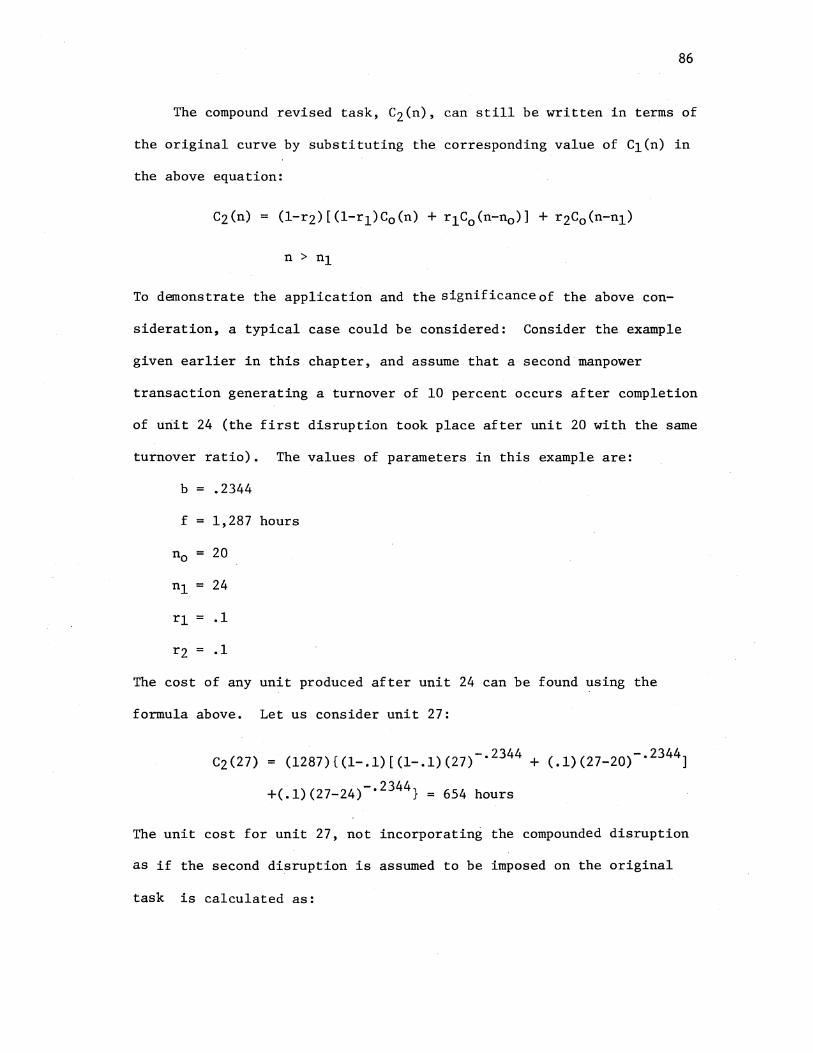
86

The compound revised task, C2(n), can still be written in terms of

the original curve by substituting the corresponding value of C1(n) in

the above equation:

To demonstrate the application and the significanceof the above con-

sideration, a typical case could be considered: Consider the example

given earlier in this chapter, and assume that a second manpower

transaction generating a turnover of 10 percent occurs after completion

of uriit 24 (the first disruption took place after unit 20 with the same

turnover ratio). The values of parameters in this example are:

b • 2344

f 1,287 hours

n0 = 20

r2 .1

The cost of any unit produced after unit 24 can be found using the

formula above. Let us consider unit 27:

c2(27) = (1287){(1-.1)[(1-.1)(27)-· 2344 + (.1)(27-20)-· 2344 ]

+(.1)(27-24)-· 2344 } = 654 hours

The unit cost for unit 27, not incorporating the compounded disruption

as if the second disruption is assumed to be imposed on the original

task is calculated as:

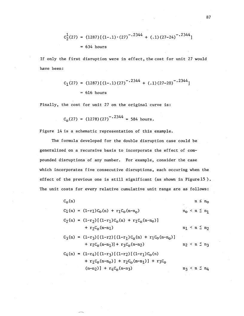
87

C~(27) = (1287)[(1-.1)•(27)-· 2344 + (.1)(27-24)-· 2344 ]

= 634 hours

If only the first disruption were in effect, the cost for unit 27 would

have been:

Cl(27) = (1287)[(1-.1)(27)-· 2344 + (.1)(27-20)-· 2344 ]

= 616 hours

Finally, the cost for unit 27 on the original curve is:

-.2344 C0 (27) = (1278)(27) = 584 hours.

Figure 14 is a schematic representation of this example.

The formula developed for the double disruption case could be

generalized on a recursive basis to incorporate the effect of com-

pounded disruptions of any number. For example, consider the case

which incorporates five consecutive disruptions, each occuring when the

effect of the previous one is still significant (as shown in Figurel5 ).

The unit costs for every relative cumulative unit range are as follows:

C0 (n) n $. no

Cl(n) = (l-rl)C0 (n) + rlC0 (n-n0 ) n0 < n < nl -c2(n) = (l-r2)[(1-rl)C0 (n) + rlC0 (n-n0 )]

+ rzC0 (n-nl) n1 < n < nz -C3(n) = (l-rJ)[(l-r2)[(1-rl)C0 (n) + r1C0 (n-n0 )]

+ r2C0 (n-n1)]+ r3C0 (n-n2) U2 < n < n3 -C4(n) = (l-r4)[(1-r3)[(1-r2)[(1-rl)C0 (n)

+ rlC0 (n-n0 )] + r2C0 (n-n1)] + r3C0

(n-n2)] + r4C0 (n-n3) n3 < n < n4 -

~

z :::> ..........

(f) 0:: :::> 0 I

654 634 616 584

20 24 27 UNIT

Figure 14. Graphical Illustrations of the Example of a Double Disruption Case

88

Cs(n) = (1-rs)[(l-r4)[(1-r3)[(1-rz)[(l-rl)C0 (n)

+ r1C0 (n-n0 )] + rzC0 (n-nl)l + r3C0 (n-nz)]

+ r4C0 (n-n3)] + r5C0 (n-n4)

It should be noticed that all revised curves are interpreted in terms

of the original curve. The original curve reflects the cost of

any unit according to the basic formula:

89

Therefore, given the slope of the applicable learning curve and the cost

of the first unit, cost calculations can be performed for any desired

unit.

The block cost the compounded disruption case can be found for

any range of the cumulative units by integrating the applicable revised

unit costs over the desired range. For example, for the range (A-B)

shown in Figure 15 , where n0 < A < n1, and n1 < B < nz, the block cost

will be:

nl L c1 (n) + A

B

B

I n1+l

+ rz L Co (n-nl) n1+1

(1-q)

B

Co(n) ·+ rl L n1+l

At this point the effect of disruption in productivity rate, as a

result of occurences of manpower transactions,has been analyzed

sufficient!~ This provides the basic tools for incorporation of

dynamic productivity consideration into the aggregate planning problem.

1-z :::>

' CJ) a:: :::> 0 :r:

Co{n)

n0 A n1 . B

Figure 15. A Typical Multiple Compounded Disruption Situation

UNIT

\.0 0

91

The succeeding sections of this chapter will present the methodology

developed for the joint consideration of the disruption effect and the

aggregate planning problem.

Aggregate Planning and Disruption Effect

Proper determination of the average productivity rate applicable.

to each period in the planning horizon of an aggregate plan, necessi-

tates the following input elements:

1. Specifications of the learning curve applicable to the firm, C0 (n)

2. Cumulative number of units produced by the firm until the beginning of the planning horizon, cum0 , and the initial workforce level, W0

3. Production rate scheduled for each period in the planning horizon, Pt, Pt = 1, 2, . . . ' N

4. Workforce level scheduled for each period in the planning horizon, Wt, Wt = 1, 2, . . . ' N

5. Values of the parameters to be used in translation of man­power index into task turnover ratio, K1, K2 and K3

6. A chosen minimum unit cost difference ratio level above which the carried-over disruption effect is considered significant, E.

Task turnover ratios at the beginning of each period can be determined

using initial workforce level and elements (4) and (5) above.

When the effect of compounded disruption is ignored, the original

improvement curve and the possible task turnovers at the beginning of

each period, along with cumulative number of units produced before and

after the period provide the necessary information for determining the

block cost for the period in question. This block cost is then divided

by the number of units produced during the peried, Pt , resulting in

the appropriate average productivity applicable to that period.

92

In order to incorporate the effect of compound disruption, the

cumulative number of units at the end of a period, during which a dis­

ruption has been in effect, could be used to determine the unit cost

difference ratio at the end of the period. This ratio, if cpecked

against the ;selected minimum unit cost difference ratio (element

number 6 above) , indicates if there is a significant carry over and thus

consideration of compounded disruption in the succeeding period. If this

is the case, calculation of the block cost for a period may involve

consideration of a sequence of events that took place during the

previous periods. Therefore, in this situation, the calculation of

average productivity for a period is not supposed to be performed

independently from the previous periods. The proper approach in

this case would involve sequential calculations, starting with the

first period and ending with the last one.

Upon determination of the applicable cost curve for a period in

the above sequential process, a trace back to the preceding periods

must be done to search for the number of compounded disruptions, and

the units at which each disruptionhastaken place. Then a recursive

computation of unit costs is performed, starting with period corre­

sponding to the first disruption in the sequence and ending with the

current period.

An example of the application of the foregoing discussion clarifies

the approach. Figure 16 illustrates a planning horizon containing 12

periods. In this hypothetical case, all possible combinations of dis­

ruption occurences are incorporated.

Some useful definitions are:

1 2 3 4 5 6 7 8 9 10 11 12

production periods

Figure 16. Unit Cost Curve Over 12 Month Period for the Hy-pothetical Case (disruptions a,re caused by manpower level changes occuring at the beginning of related periods.)

cumi - Cumulative number of units produced by the end of period i

ri - Task turnover ratio resulted from manpower transaction at the beginning of period i

INDEXi - 1 if the disruption effect at the beginning of period i is significant ri ~ Kz

o.otherwise

94

ICHKi - 1 if the unit cost difference ratio at the end of period i is large enough to indicate a carried-over effect, UDR(cumi) ::: e:

0_, otherwise

Using the original unit cost curve, equations developed for

single and compounded disruption cost effects, and the approach dis-

cussed in this section, the unit cost curves applicable to those con-

ditions depicted in Figure 16 are listed in Tableiii.

Some of the unit cost functions in this table have not been ex-

panded in terms of the original curve. For period 4, for example, the

expanded cost function is:

These equations are used in the recursive computations that are per-

formed to obtain the unit cost where the compound disruption is in effect.

The values of ICRKi are determined by simply substituting cumi

in place of n in the respective unit cost function. The block cost

for period i is found by integrating the cost function applicable to

the period from cumi-l + 1 to cumi· This block cost is then divided

by Pi to obtain the average productivity applicable to the period.

Values of Pi, Wi and average productivities in every period along with

TABLE III

UNIT COST FUNCTIONS FOR THE EXAMPLE DEPICTED IN FIGURE 16

Period INDEX ICHK Unit Cost Curve Applicable Unit Range

1 0 0 C1(n) = c0 (n) cum0 < n :::; cum1

2 1 1 c2 (n) = (l-rz)C0 (n)+rz·C0 (n-cuml+l) cum1 < n :::; cumz

3 1 1 C3(n) (l-r3)Cz (n)+rJ•C0 (n-cumz+l) cumz < n ~ CUffi)

4 1 1 C4(n) = (l-r4)C3(n)+r4•C0 (n-cum3+l) CUffiJ < n s: cum6

5 0 1 Cs(n) C4(n) CUffi) < n s: cum6

6 0 1 C6(n) C4(n) CUffiJ < n ~ cum6

7 1 1 C7(n) (l-r7)C4(n)+r7·C0 (n-cum6+l) cum6 < n ~ cum7

8 1 1 ca(n) (l-rs)C7(n)+rs·C0 (n-cum7+1) cum7 < n ~ cum1o

9 0 1 C9(n) - c8 (n) cum7 < n ~ cum10

10 0 1 clo(n) = c8 (n) cum7 < n ~ cumlo

11 1 1 c11 (n) (l-r11)c8 n)+rll·C0 (n-cum11+l)cumlo < n :::; CUID12

12 0 1 c12 (n) = C11(n) -cum1o < n :;;;. cum12

96

other parameters in the cost function are used to obtain the total cost

of this specific aggregate plan.

Optimization Methodology

In the previous section the methodology for evaluating the per­

formance of a 'specific' aggregate plan under dynamic productivity

condition was presented. A specific aggregate plan was recognized by

the specific levels of production and workforce at each period of the

planning horizon. Theindex of performance of such a plan is the total

cost level resulting from the plan.

Production and workforce levels are the independent, or controllable,

decision variables in this operations planning problem. These decision

variables can be adjusted within specified boundaries so as to produce

the best possible index of system performance (the minimum level of

the total operating cost). Therefore, application of a search technique

would involve systematic adjustments of the levels of decision variables

and exploration of the response surface. The optimum solutions are

those which correspond to the minimum response.

The structure of the cost function in the constant productivity

models is fixed and independent of the levels of decision variables.

However, in a model which incorporates dynamic productivity,

this structure is totally dynamic in nature because the productivity

coefficients are not constant throughout the planning horizon. These

coefficients are related to the levels of decision variables; therefore,

they form a new structure for the objective function every time an

adjustment in these levels is made. It is conceivable that in such

a dynamic system, sensing the performance of a specific set of values

for decision variables would necessitate the determination of the

respective structure of the objective function first and then evalua­

tion of the response against these levels for decision variables.

The optimization methodology proposed for the current model is

based upon the above considerations, and is composed of three inter­

acting major units.

The first unit is the pattern search routine, called PATS. As

demonstrated in the diagram in Figure 17 , this routine generates a

sequence of levels for decision variables, workforce and production,

in every period in the planning horizon.

97

The second unit is a routine, called PROTCV which receives the

information generated by PATS and utilizes the approach discussed in

the previous section. This routine generates unit cost curves appli­

cable to each period on the basis of the input information about the

magnitudes and patterns of ups and downs in the levels of workforce and

production throughout the planning horizon. Based on the unit cost

curves, this routine then determines the appropriate average productiv­

ity levels applicable to the respective periods.

The third routine, called FCTl, receives the information generated

by PROCTIV and forms the updated structure of the objective function.

This routine evaluates the response of the newly structured cost func­

tion against the corresponding levels of decision variables, the levels

originally generated by the PATS routine.

The response evaluated by FCTl routine is fed to the PATS routine.

The magnitude of this response provides the search routine with the

necessary information to make appropriate adjustments in the level of

decision variables. The newly adjusted levels are fed to the PROCTV

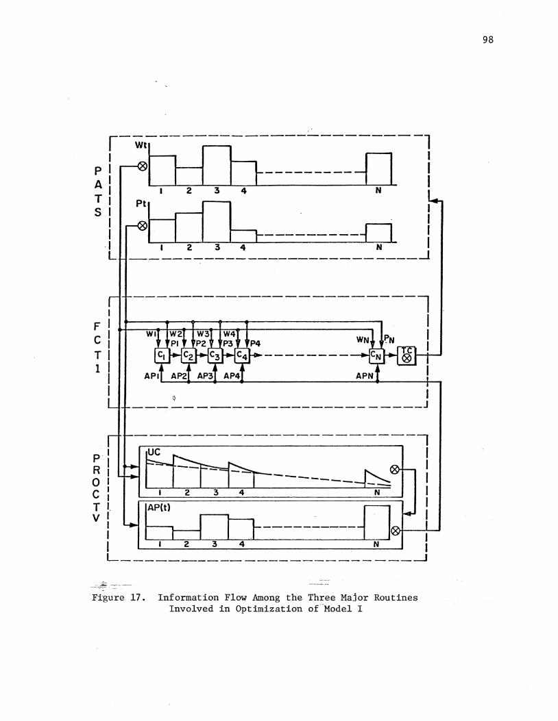
~-Wt----------------------1

pi b I b---------n i AI I 2 3 4 N

~ i Ptl I b----------0 ·I I 2 3 4 N I L ---------------------------~

I Fl c' I Tl 1 I

I

p R 0 c T v

I

-----------------------l

I I I

Q I _________________________ j

lAP( I)

Frgure 17. Information Flow Among the Three Major Routines Involved in Optimization oCModel I

98

routine and the whole process is continued until the optimum solution

is found.

99

A considerable increase in the amount of computation time occurs

when incorporating the dynamic productivity considerations into the SDR

solution technique, since .for every proposed change in the level of

decision variables made by PATS a call is made to the PROCTV routine.

For example, using a 10-period planning horizon, the optimization of a

cost function similar to the paint factory model would, on the average,

involve 3000 evaluations of the objective function. For each evalua­

tion the PROCTV routine performs a sequence of computations similar

to those presented in Table II. A considerable portion of these com­

putations can be avoided and, therefore, a considerable time saving

could be achieved, if the procedures described below are used.

One of the. major factors affecting the number of required evaluations

in all search routines is the starting solution vector. The closer this

initial solution is to the optimum, the fewer evaluations required to

reach the optimum. Therefore, a procedure which would approximate the

optimum solution can always provide a better starting point than a

starting point chosen intuitively. For the dynamic productivity model,

this procedure could be the one which optimizes a somewhat equivalent

average productivity model. Since the cost structure in this model is

fixed, the optimization process would involve a considerably small com­

putation process, and therefore a considerably smaller computation time.

The dynamic productivity model could then utilize this optimal solution

as a starting point and proceed toward its own optimum. The efficiency

of the solution technique can be improvedfurther, if an intermediate

model, which incorporates the improvement curve but not the disruption

100

effect (Ebert model), is utilized. In this setting, a starting solution

vecto.r would be chosen for optimizing the constant productivity model.

The optimum solution to this model is then utilized as the starting

point for the intermediate model, and the solution to the intermediate

model can serve as a starting solution to the final complex model. In

this approach, each model represents the real situation more realistically

than its preceding one.

Besides saving computation time, the above procedure also provides

information regarding the comparative performances of the three models

under different situations.

Further improvement in the computation efficiency is still possible

by improving the efficiency of the algorithm utilized in the PROCTV

routine. A great portion of the computations can be avoided in this

routine by observing the fact that average productivites do not have to

be computed for all periods every time the level of a decision variable is

adjusted. It should be noticed that the average productivit;y at a given

period could only be related to the levels of decision variqbles in

the preceding periods that is, a change in the level of workforce,

or production at a given period can only affect the average productiv­

ities in the succeeding periods. For example, in a 20-period model, a

change in the workforce level at period 18, W1s, can only affect the

average productivities inperiodsl8, 19 and 20. The average productiv­

ites for the first 17 periods would remain unaffected. Therefore, a

check can be made at the beginning of the PROCTV routine to determine

the first period for which a decision variable has changed. The com­

putation steps should then be carried on only for the current and the

succeeding periods.

101

The above provisions are all incorporated into the optimization

procedure used in this study. A more detailed explanation of this

procedure follows.

Procedure

Figure 18 illustrates a block diagram of the optimization procedure.

Glossary of code definitions, flow charts and the documented program

listing for this procedure are provided in Appendixes A, D and E,

respectively.

The main program reads the model parameters and initializes the

search routine. The computation of the overall average productivity for

the equivalent constant productivity model is performed in this routine.

This average productivity is determined by applying the original improve-

ment curve and computing the block cost for units ranging from cumo

(the cumulative production by the beginning of the first period) to N

cum0 + I Di (Di being the demand level for period i). i=l

The PATS routine is then called and the constant productivity model

is optimized and the results are printed. The optimum solution of this

model is then fed into PROCTV through a call to FCTl. This evaluates

the performance of the constant productivity model in situations where

the dynamic productivity condition is present. The result of this

evaluation is then printed.

A similar set of steps is then followed for the optimization and

evaluation of the optimum solution to the Ebert model, the starting

solution vector for this optimization being the optimum solution to the

first model. The optimum solution to the second model is then utilized

as the starting solution for the optimization of the dynamic productivity

MAIN ----•

,

PATS

~

r

.. FCTl -•

r

- .. -UNIT PROCTV BLOCK .. .. -

Figure 18. Block Diagram of the Optimization Procedure for Model I

102

103

model. This model is optimized and the results are printed. In summary,

the outputs of this routine are: the optimum plan and corresponding cost

level for the constant productivity model; the cost of implementing this

plan in a changing productivity situation; the optimum plan and corre­

sponding cost levels for the Ebert model; the cost of implementing this plan

in a changirlg productivity situ~tion; and the optimum plan for the:dynamic pro­

ductivity model and the associated cost levels. Appendixes C and F should

provide a complete description of the pattern search subroutine calles PATS.

Subroutine FCTl increments the number of function calculations,

receives the levels of the decision variables from PATS and directs

these levels to PROCTV to receive back the applicable productivity

levels. The structure of the cost function is updated, different cost

elements are calcualted for every period and the total cost is reported

to PATS from this routine. FCTl also computes and incorporates the

penalty of violating the model constraints.

Subroutine PROCTV starts with detecting the effective period: the

first period at which the value of a decision variable does not corre­

spond to its previous value. Recognition of types of manpower trans­

actions, computation of manpower ratios, translation of these ratios

into the equivalent task turnovers, and setting of the disruption index

for each period are then performed. Next, unit and block cost computa­

tions for periods with no disruption and single disruption are performed.

The carried-over disruption index, ICHK(I), is also set for all periods.

The recursive computations for compound disruption effects are performed

where applicable. Finally, the values for average productivity levels

applicable to each period are computed and reported back to the FCTl

routine.

104

PROCTV interacts with two function routines UNIT and BLOCK, which

compute unit cost for every proposed cumulative unit and block cost for

every proposed range of cumulative units, respectively. Computations

performed by these routines are based on the original improvement curve,

C0 (n), for the given unit number as requested by PROCTV.

The above procedure performs the month one optimization. To

perform the next month optimization (at the beginning of the second

month, and for a revised forecast) the effect of possible disruption

resulting from implementing the month one decisions and possibly con­

tinuing through month two is to be considered. The value ofthe unit

cost difference ratio at the end of month one provides the information

regarding this effect. Therefore, for the beginning of the second

month (in the month two optimization), this value can be added to the

turnover ratio resulting from the possible disruption at this period.

The optimization procedure is then the same as before for all periods

in the planning horizon.

Remarks

Based on the foregoing analysis of disruption effect on the pro­

ductivity factor in the aggregate planning, Figure 19 demonstrates a

hypothetical situation in which the periodical average man-month

requirements per unit product (the inverse of average productivities)

considered by the constant productivity models, the Ebert model and

the dynamic productivity model (new model) are contrasted.

This figure shows that while the Ebert model assumes a continuously

increasing average productivity, the new model considers a fluctuating

average productivity level. The figure also qemonstrates the fact that

---- CONSTANT PRODUCTIVITY MODEL

-·-·- EBERT MODEL -- DYNAMIC PRODUCTIVITY MODEL

2 3 4 5 6 7 8 9 10 II 12 production periods

FigurP 19. Comparison of the Patterns of the Man-month Requirements per Product Unit (inverse of average productivity) in Constant Productivity, Ebert, and Dynamic Productivity Models for a Hypo­thetical Situation

106

disruptions occuring further in the production sequence impose.more

significant effects on the average productivity level; the difference

between the average productivity levels considered by the Ebert model

and the new model becomes larger in the further periods. As will be

seen in Chapter VII, the analysis of the results numerically support

the relevance of the ideas depicted in this figure.

CHAPTER VI

MODEL II. SHORT CYCLE PRODUCTS

Introduction

Most mass production and make-to-stock type of operations can

be classified as the short cycle operations. Unlike the case of

long cycle products, in the short cycle operations the unit output

rate of the firm can be rather directly attributed to the productivity

rates of the individual workers.

Short cycle operations are usually uncomplex and are composed of

·few tasks, all being performable by an individual employee, or by a

small number of employees sequentially performing specific tasks.

Even though processing of a shortcycleproduct unit may require

utilization of more than one employee, the short cycle operation is

not a team activity of the type found in long cycle operations. This

is due to the independency persisting among the work segments per­

formed by different employees.

There are several consequences of this special nature of the

short cycle operations. For example, the primary step for coordination

is the choosing of employees with similar productivities when arranging

a crew for a production line. The pace of the production line is

always limited by the slower members in the sequence, and because of

the independency of work, any improvement found by some members does

107

108

not help the others. Short cycle activities usually involve a number

of small production lines each utilizing a homogeneous class of

employees. When a need arises for production rate changes through

changes in the workforce level, a number of production lines are

either dropped or added. A decrease or increase in the workforce

level is not usually accompanied by the reassignment of manpower;

therefore, disruptions in the average productivity level do not per­

sist as a result of such transactions. Any drop in the overall

average productivity level of the firm is due to the addition of

slower production lines utilizing newer employees.

It is only in the above organizational settings, that the

assumptions regarding experience classes considered by Orrbeck et al.

are justifiable. In considering plans for long cycle operations it

is conceivable that these assumptions are far from being realistic.

The objective of this chapter is to develop an aggregate produc­

tion planning model suitable for the firms manufacturing short cycle

products with special attention devoted to the proper incorporation of

the dynamic productivity phenomenon. The new model incorporates some

basic assumptions of the Orrbeck et al. model; however, the general

approach in the model development and the solution methodology utilized

are totally different and new in nature. Direct application of

improvement curve analysis with detailed reference to learning,

progress and retrogression effects form the essence of the new model.

A number of interesting and significant facts about the nature of the

objective functions in most aggregate planning models are highlighted

as the outcome of this part of research. A detailed explanation of

this research will follow in suceeding sections of this chapter.

109

Analysis of the Effect of Manpower Changes

As it was mentioned previously, in the case of short cycle products,

disruption in productivity as a result of task reassignment is not

usually experienced. Even for major crew expansion or reduction, re­

shuffling of tasks such that some experienced workers wind up with

brand-new reassignments is not expected to occur; however, lack of

such a disruption effect does not mean that manpower transactions do

not generate significant effects on the overall average productivity

level of a short cycle manufacturing firm.

Implementation of the decisions generated by the aggregate plans

may require constant addition of untrained people and loss of trained

ones for almost every type of manufacturing firm. These transactions,

coupled with fluctuating production output requirement per period

result in fluctuating average productivity levels over the periods

of the planning horizon. For the short cycle case, the addition of

production lines with slower paces, or the shutting down of faster

lines as a result of additions or reductions in the level of work­

·force are the natural causes for such fluctuations.

Fluctuations in the level of workforce result in constant

generation of new experience classes, or they vary the number of such

classes. However, workforce fluctuations are not the only factors

affecting the number and the sizes of the experience classes in dif­

ferent periods.

According to the learning curve analysis, an employee's produc­

tivity is a function of the cumulative units produced by that employee,

and (as will be discussed later) this productivity is also a function

of the "progress" attained by the firm. On the other hand, the options

110

of overtime and. idle time, which are frequently utilized by firms and

indicated by aggregate plans, can generate situations where groups of

employees starting at identical productivity levels may end up producing

different cumulative product units after one or more periods. Therefore,

the alternative ways of workforce utilization affect the conditions of

experience classes in different production periods.

j:t- One basic distiction between the new model and the Orrbeck et al.

model arises from the above point; that is, the new model recognizes

the alternative ways of workforce utilization as a factor affecting

the conditions (number of classes, size,and productivity) of the

experience classes. As will be shown later, other significant distinc-

tions between the two models ·do exist. The foregoing considerations

structure the assumptions of the new model.

Assumptions of the.New Model

The new model adapts the assumptions regarding the effect of

workforce fluctuations through hiring and layoff, considered by

Orrbeck et al. The assumptions governing the assignment of overtime

are also adapted from this model. The basis for recognition of the

experience classes in the new model is the productivity rates of the

members of each class based upon the cumulative number of product

units experienced by those members. Other factors affecting produc-

tivity rates are the ones associated with the progress effect and the

retrogression effect.

It should be noted that the new assumption differs in nature from

the one adapted by Orrbeck et al. who relate the productivity rates

to the passage of time. They relate the productivity rate of each

111

experience class to the time span during which the experience class is

involved in the firm's activity. Such relationship may exist only if

workers are utilized on regular time, a situation which is indeed unreal­

istic. Based upon the new assumptions presented above, each element of

the new model and the logical relationships among the elements are

analyzed in the following sections.

Workforce Fluctuations

Fluctuation in the workforce level is an element which affects

the conditions of experience classes according to the assumption employed

by Orrbeck et al. That is, the least experienced class is the one which

consists of the newly hired workers. If workers are to be fired, the

least experienced workers are fired first. Should the number of people

fired in a period exceed the number of employees in the least experi­

enced class of the previous period, some workers from the next least

experienced class would have to be laid off.

Not including the effect of all other relevant factors (which will

be explained in the later sections), the effect of workforce fluctua­

tions on a typical situation is demonstrated in Figure 20. In this

hypothetical case, a planning horizon consisting of six periods is

considered. Originally, the first period includes three experience

classes. In Figure 2~b rectangulars with lower numbers indicate

experience classes with higher productivities. A typical fluctuation

pattern in the level of workforce, as shown in Figure 20.a affects the

conditions of experience classes as shown in Figure20.b.

..J lLJ > lLJ ..J lLJ 0 0:::

~ ~ 0::: 0 3:

I I I

2 3 4 I I

5

a.) PRODUCTION PERIODS

..J lLJ > lLJ ..J

lLJ () 0:::

f2 ~ 0:: 0

==

I

2

3

I I

2 I 2

3 2. 3 I

4 3 4 2 5 2 3 4 5

b.) PRODUCTION PERIODS

6

I

2

3

4

6

Figure 20. Effect of a Typical Manpower Level Change on the Conditions of Experience Classes

112

113

Regular Time

The new model assumes that regular time work is assigned to workers

in order of their seniority. Thus, the most experienced workers will

work on regular time first subject to the limit of their capacity. If

regular time work still remains, the next most experienced class will

be utilizied; and similarly, the remaining experience classes will be

utilized until all regular time work is assigned.

There are two possible outcomes of the above situation. First,

if the amount of regular time work is smaller than the production capability

of all experienced classes, some lower experienced workers will remain

idle. (This is a realistic situation that Orrbeck et al. do not

incorporate in their model.) Second, if the amount of regular time

work exceeds the total production capability of all experience classes,

the excess production must be performed on overtime. Should this excess

amount exceed the production capability of all experience classes on

overtime, subcontracting might be utilized. If a particular'situation

does not include the possibility of utilization of subcontracting, then

the model will indicate the infeasibility of the planned production rate

in the appropriate period. It should be noted that Orrbeck et al. do

not include considerations regarding the subcontracting option. Their

model does not incorporate the constraint relative to the production

capability on overtime. They first establish an upper limit on the

production that can take place on regular time, and then they assume

any production in excess of this amount must be done on overtime.

Based upon the assumptions of the new model, the analysis of

regular time work and its effect on the condition of experience classes

114

would require the following input information for each period:

Production rate scheduled for the period

Workforce level scheduled for the period

Number of experience classes, size and measure of productivity of each experience class at the beginning of the period

Given the current scheduled workforce level and the workforce level in

the preceeding period, the condition of the experience classes in the

current period can be revised by applying the approach discussed in the

previous section.

To remain consistent with the improvement curve theory, the cumula-

tive output unit per employee in a given class can be chosen as the

"measure of productivity11 of that experience class. Given the total

production rate scheduled for the given period, and also given the

number of experience classes, size and productivity measure of each

class, the total number of men to be assigned on regular time work can

be determined. This is possible by first finding the production

capability of each experience class during regular time, and then com-

paring the total of the production capabilities with the total scheduled

production rate for the period.

The production capability of an experience class can be found usinga

revised form of the block cost expression discussed in the analysis of linear

learning curves. According to this expression, the total man-months

required to produce units nl through nz is given by:

nz l C(n) = 1 : b [(nz + .5)(l-b) - (n1 - .5)(1-b)] nl

(6.1)

For simplicity, ignoring the approximation improvement factor .5 in the

above equation, the formula will reduce to:

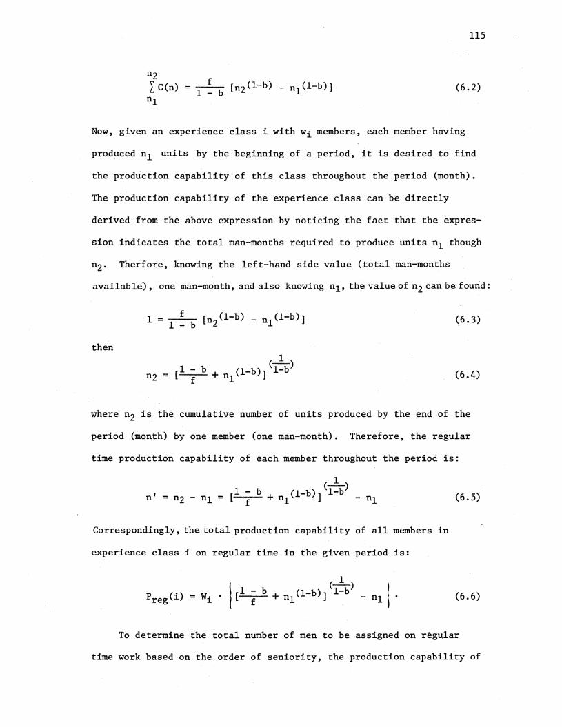
nz L C(n) nl

115

(6.2)

Now, given an experience class i with wi members, each member having

produced n1 units by the beginning of a period, it is desired to find

the production capability of this class throughout the period (month).

The production capability of the experience class can be directly

derived from the above expression by noticing the fact that the expres-

sion indicates the total man-months required to produce units n1 though

nz. Therfore, knowing the left-hand side value (total man-months

available), one man-mo"nth, and also knowing n1 , the value of n2 can be found:

then

1 f [ (1-b) (l~b)] = 1 - b n2 - nl

(-1-) nz = [1; b + nl(l-b)] 1-b

(6.3)

(6. 4)

where n2 is the cumulative number of units produced by the end of the

period (month) by one member (one man-month). Therefore, the regular

time production capability of each member throughout the period is:

(6.5)

Correspondingly, the total production capability of all members in

experience class i on regular time in the given period is:

(6.6)

To determine the total number of men to be assigned on regular

time work based on the order of seniority, the production capability of

'1

116

the first experience class (the highest experienced class) is com-

pared against the scheduled production rate Pt for the period in ques­

tion. If the production capability of this .class is smaller than Pt,

the excess amount is compared against the production capability of the

second experience class. The comparison process continues until one

of three outcomes occurs.

First, if the excess production amount left for the last experience

class (with the lowest productivity) exceeds the production capability

of this class, the excess amount must be done on overtime. If the

total production capability in overtime is smaller than this amount,

the excess must be retained through subcontracting (if possible). This

case will be explained in more detail in the next section.

Second, if the comparison process of the excess production amount

against the production capability of sequentially considered experience

classes continues until the production capability of an experience class

equals (within an acceptable tolerance) the excess production amount,

the current class and all higher classes are assigned on regular

time work. The productivity measure of the members in these classes

is increased by their respective production capabilities during the

given period. This updates their status for the beginning of the next

period. In this case all succeeding experience classes (the ones with

lower productivities than the current one) will remain idle. The

detailed treatment of productivity status of the members of such

classes will be explained later in a related section.

Figure 21 illustrates the latter situation. In this figure a

workforce level Wt is comprised of five different experience classes.

The total production scheduled for the period Pt is compared against

production capability of experience class 1, Preg(l). The remainder

.... _ -

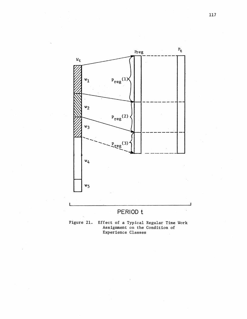
Preg

- ..... _ p (3) ..... reg ----

PERIOD t

Figure 21. Effect of a Typical Regular Time Work Assignment on the Condition of Experience Classes

117

118

of production is compared against PregC2) and the comparison is contin­

ued until the last remainder of Pt is found to be equal to the produc­

tion capability of the third experience class. In this case the

shaded portion of wt indicates the workforce assigned on regular time.

The unshaded portion shows the classes which are left idle.

The third possible outcome of the comparison process is the situa­

tion where the procedure continues until the production capability of

an experience class exceeds the remaining production amount. In such

case, the ratio of the excess amount over the production capability of

the experience class in question can indicate the portion of the class

which will remain idle (this is true because all members in a class

have similar productivity rates). All other remaining classes with

lower productivities will also remain idle. It should be noted that in

this situation, an experience class is broken into two parts. One

which is assigned on regular time work, and the other which remains idle.

As a result of such a transaction, the two segments would represent two

different productivity rates at the beginning of the next period; one

part gains productivity through producing more units during regular

time work, the other part loses some productivity due to the retrogres­

sion effect. Therefore, productivity measure of each of the working

experience classes is increased by the number produced by each member

during the period and the status of these classes is updated. The

status of each of the idle classes is also updated, using the analysis

of retrogression effect (to be discussed later).

Figure 22 illustrates the above situation. In this hypothetical

case, the comparison process has continued until it is found that the

third experience class is capable of producing more than actually

w t

p (1) reg

PERIOD t

Figure 22. Effect of a Typical Regular Time Work Assignment On the Conditions of Experience Classes, Creating a Partitioned Class

119

120

remains to be produced. The ratio of the excess amount Px, over Preg(3)

quantifies the partition of this class into two new classes: the working

class comprising wj members, and the idle class comprising w~ members.

This case shows that number, size and productivity level of each exper­

ience class can be affected by the regular time assignment of work.

At this point, it must be mentioned that an alternative assumption

regarding the latter case may be relevant in some situations: When the

production capability of a class exceeds the production amount scheduled

for the class, the work may be equally distributed among the members

of the class, thereby allowing undertime work for all members in the class.

This assumption would considerably simplify the analysis; for in this

case, the class is not partitioned and the number of classes and the size

of each class would remain unchanged. The productivity measure of each

member receiving undertime work would increase by his share of work. This

assumption is not incorporated in the present model.

OVertime

Overtime is utilized whenever the production level scheduled for

a period exceeds the total production capability of all employees on

regular time. The analysis of the overtime effect is very similar to

the one applied to the regular time. This analysis is based upon the

assumption of Orrbeck et al. regarding the assignment of overtime.

That is, when overtime is used, workers will be called upon in order of

seniority. Thus, the most experienced workers will work overtime first

subject to the limit of their capacity. If overtime work still remains,

the.next most experienced class will be called upon; and similarly for

the remaining experience classes until all overtime work is assigned.

121

Since the analysis of overtime work is conducted after the inclusion

of the effects of workforce fluctuations and the regular time utilization,

the only information required for this part of the analysis for each

period is:

J

Remaining production after the assignment of regular time work

Number of experience classes, size and the cumulative number of units experienced by the members in each class

The length of overtime as a percentage of the length of regular time

Given the remaining production amount, and also given the number of

experience classes, size and productivity measure of each class, the

total number of men to be assigned on overtime work can be determined

by finding the production capability of each experience class during

overtime, and comparing the result with the remaining production amount.

The production capability of an experience class can be determined

by applying the same revised form of the block cost expression which

was applied in regular time analysis. The only difference between the

two cases is that the overtime duration is usually smaller than the

duration of regular time.; therefore, if one man can represent one man-

month worth of work during regular time, this man can only provide a

proportion of a man-month work during overtime. If overtime is assured

to be as long as a percent of regular time in a period, then Equation

(6.3) can be written as:

a•l = 1 ~ b [m2 <1-b)- m1 (1-b)] (6. 7)

In this expression, m1 is the cumulative number of units produced by

the employee by the beginning of the period, and mz is the expected

122

cumulative unit that will be produced by him during overtime by the end

of the period.

In a given period, an employee is assigned on overtime only if he

is also assigned on regular time. This indicated that there is an

interactive effect between productivity improvements during regular

time and overtime. Overtime work is performed during the same day

that regular time has been performed. The experience gained during

regular time would effect the productivity during overtime. Precise

incorporation of this interactive effect requires the breaking of each

period into the number of days contained in each period. However, such

division would result in a large amount of increased computational

time, while the gained precision in the short length of one period

(compared to the length of the planning horizon) may not deviate too

much from an approximated quantity. This approximation can be done

by improving the productivity measure in Equation (6.7). To do this

the value m1 in this equation is set equal to the total of: (1) the

cumulative units produced by the beginning of the period, and (2) one-

half (average of the total regular time production at the beginning and

at the end of the period) of what is produced during regular time:

n' ml = nl + T

The variable, n', is the total units produced by a member. during

(6 .8)

regular time in the same period, and is computed using Equation (6.5).

Using Equation (6.7), the overtime production capability of each

member with productivity measure of m1 (at the beginning of the period)

throughout the period is:

123

1

m' = mz - ml [CI.( l-b) (1-b) (1-b) = f + ml ] - m1 (6.9)

The total production capability of the ith experience class consisting

of wi members, each with productivity measure of m1 is, therefore:

1

Pover(i) = wi I [a(l;b) + ml (1-b)] (1-b) - liiJ.I (6.10)

To determine the total number of men to be assigned on overtime

work in a given period (t), first the total amount of overtime work is

computed by deducting the total regular time capabilities of all classes

from the production rate scheduled for the period. Denoting this

remaining production amount by RPt, then RPt = Pt- ~ Preg(i). Based l.

on the order of seniority, the overtime production capability of the

first experience class is compared with RPt. If the overtime production

capability of the first class is smaller than RPt, then the excess

amount is compared against the overtime production capability of the

second class. The comparison process continues until one of three

possible outcomes occurs.

First, if the excess production amount left for the last experience

class exceeds the production capability of this class, then the excess

amount must be retained through subcontracting. If, for a specific

situation, the subcontracting option is not available, then in the

above case an infeasible schedule must be reported. This is true

because,in this situation, the scheduled production for the period in

question cannot be met even if all employees are fully utilized (both

on regular time and overtime).

Second, if the comparison process of the excess production amount

against the overtime production capability of the sequentially taken

124

experience classes continues until the production capability of an

experience class equals (within an acceptable tolerance) the excess

production amount, the current class and all preceeding classes are

assigned on overtime work. The productivity measures of the members

in these classes are increased by their respective production capabil­

ities during the given period. This updates the status of each class

for the beginning of the next period. In this case,all succeeding

experience classes are only assigned on regular time and, since this

assignment is done prior to consideration of overtime, the status of

these classes will remain unchanged.

The third possible outcome of the comparison process is the situa­

tion where the production capability of a class in sequence exceeds the

remaining production amount. In such case (like the similar case in

regular time considerations) the ratio of the excess amount over the

production capability of the experience class involved can indicate

the portion of the class which is not assigned on overtime. Therefore,

an increase in the number of experience classes will result as a

consequence of such a situation. The two newly generated classes

will differ in the relative productivity measures at the beginning of

the next period. Due to the assignment of overtime, the first class

will gain higher productivity as compared to the second one, which

only performs regular time work.

Figure 23 illustrates the above situation. In this hypothetical

case the comparison process has continued until it is found that the

third experience class is capable of producing on overtime more than

what remains to be produced. The ratio of the excess amount RPx, over

P0ver(3) is used to partition this class into two new classes: the

Povr

PERIOD t

= Pt - I Preg(i) i

Figure 23. Effect of a Typical Overtime Work Assign­ment on the Conditions of Experience Classes, Creating a Partitioned Class

125

126

upper part consisting of w~ members assigned on overtime, and the lower

2 part consisting of w3 members assigned only on regular time. The double

shaded areas in Figure 23 represents those classes assigned both on

regular time and overtime.

It should be noticed that the assignment of overtime is another

factor affecting number, size and productivity of experience classes

involved. In addition, the analysis applied in this section directly

determines the total number of workers assigned on overtime for any

given period. This number, if incorporated into the total cost function

as a variable, can improve the degree of realism of the function; there-

by eliminating the possiblity of generating unrealistic results such

as the 'negative overtime' indicated for some periods by the HMMS model

in the paint company example.

Idle Time

As discussed earlier in the chapter, if in any production period

the total regular time production capability of workers exceeds the

production rate scheduled for the period, some workers would remain

idle. Devotion of special consideration to this phenomenon seem to be

necessary because of at least two reasons: first, the idle time pay-

ment in some firms is estimated separately and is different from the

regular time and the overtime payments. Therefore, inclusion as a

variable the number of idle workers in each production period in

the cost function of the aggregate planning model would improve the

degree of realism of the function. Secondly, the assignment of idle

time generates a decay in the productivity rate of the workers

involved. This is due to the forgetting effect experienced during

127

idle time. In the literature of learning curve analysis this effect

is usually referred to as retrogression or interruption effect. It

was noted that the analysis of regular time also revealed the number

of idle workers per period: where idle time applied. This number can

be directly incorporated into the total cost function with the proper

cost coefficient.

To analyze the effectof idle time on the productivity rate of

idle workers in the aggregate planning problem the analysis of the

retrogression effects is considered. According to this analysis [19]

[17], the forgetting or interruption phenomenon can be described by

a negative decay function comparable to the decay observed in electrical

losses in condensers. If it is assumed that an individual's memory

is the equivalent of storing electrical charges in the brain, then the

decay analogy appears reasonable. In general, the amount of retrogres­

sion is a function of the quantity produced by the time that interrup­

tion occurs, and the length·of the interruption period.

Forgetting patterns show rapid initial decrease in performance

followed by a gradual leveling off as a function of the interruption

interval. Also the rate and the amount of forgetting decreases as

an increased number of units are completed before an interruption occurs.

Therefore, the forgetting pattern is very similar to a learning pattern

with negative slope. This slope is known as the forgetting slope.

Interruptions, which can take place at any point, and the number

of units produced (productivity measure) at this point together with

an assumed forgetting slope yield a model for forgetting. At the

point of resumption, the performance or unit time can be used to

determine the restart point on the original improvement curve. Figure

128

24 shows the performance versus elapsed weeks for an interrupted

operation with a learning slope of 87% and a forgetting slope of 80%.

The expected unit times for an interrupted operation can be

determined in a Learn-Forget-Learn (LFL) model by first considering

the original learning curve formula for the log linear model. The

expected unit costforcumulative unit X is given as

T(X) = Tl·X-L

where Tl is the base unit time, L is the measure of learning slope, and

X goes from unit 1 to Ql. The latter term being the unit at which the

interruption began. . .

At this point a similar model for forgetting is used to estimate

• the degradation during the interruption. The equivalent intercept (see

Figure 25) can be computed from Ul and Ql, the unit time and quantity

completed when the interruption occurred, and an assumed forgetting

slope. For example, if a forgetting slope of 80 percent was used, this

would mean that ultimately only 80 percent of what was learned would be

retained. Using the following formula:

T2 = Ul•Ql-F

where F is the forgetting slope, the intercept for the forgetting curve

can be found. The equivalent unit time at a point where learning is to

resume would be found from:

U2 = T(X) = T2•XF

This point is the equivalent unit time and quantity at which

performance has degraded over the duration of the interruption. An

interval expressed in time periods can easily by converted to equivalent

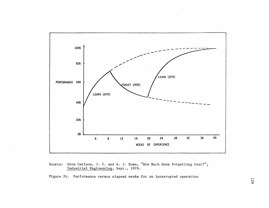
100% --------.... -..... ..... ..... ..... / 80%

/

PERFORMANCE 60%

LEARN (87%)

40% --- ----------

20%

0% 4. 8 12 16 20 24 28 32 36

WEEKS OF EXPERIENCE·

Source: From Carlson, J. C. and A. J. Rowe, "How Much Does Forgetting Cost?", Industrial Engineering, Sept., 1976.

Figure 24. Performance versus elapsed weeks for an interrupted operation

40

units in a manner similar to that employed for the learning portion

of the LFL curve.

130

Following the resumption of work, the unit times for the learning

curve could be expected to follow the original curve but displaced

back up the improvement curve to the point equalling the expected re­

start unit time. The equivalent start quantity Q3 is found from:

U3 = U2 = Tl/Q31

Figure 25 shows the expected time as superimposed back over the original

learning curve and the scallop shaped curve resulting when theseunit

times are plotted against the cumulative quantity to date.

The application of the concepts described above to the analysis of

the effect of idle time on productivity of workers in the current model

happens to be straight forward and requires fewer number of computations

than the above methodology. This is due to the fact that in the current

model, the status of the productivity measure of each experience class

is updated periodically. Therefore, if idle time is experienced, the

interval of interruption considered is always one period. For a given

period the productivity status of an idle class at the beginning of

the following period, can be. found by degrading the productivity

measure of this class (at the beginning of the current period) over an

interrruption length of one period, using the applicable forgetting

slope. If the current class is to remain idle in a number of subsequent

periods, the degrading process is then imposed sequentially on the

updated (degraded) productivity measures throughout the total interrup­

tion interval, each time considering an interruption length of one

period. If at any period work is to be resumed, the updated status of

TUif:

PER .

UNIT

T1

s

12 1

LEARN: IQll T(X}.,TliXl

FORGET:

T(X)•T2•XF

where TZ•Ul/Qlf

IQZ

Ql

RESI.Jii£ LEARN:

T(X)•Tl/(X-Q2+Q3)l

where Q3.,(Tl/U2)11l

JO

Q3 I

102

CUHUlATIYE UNITS

QZ

EXPECTED TIME tt UNIT Z

Source-: From-Carlson, G.andA. J. Rowe, "How Much Does Fo.rgetting cost?'', Industr-ial Engineering, September, 1976~ ·

Figure 25. Expected Unit Times for an Interrupted Learning Experience

131

132

each experience class would indicate the applicable startingproductivity.

To determine the quantity by which the productivity measure of an

idle employee degrades throughout one period, let us first consider

Equation (6.5) given in the analysis of regular time. This equation

actually represents the quantity by which the productivity measure

upgrades as a result of learning gained over one period. If in this

equation, the forgetting slope, F, is substituted in place of the

learning slope, b, this equation can be used to represent the quantity

by which the productivity measure degrades as a result of an interrup-

tion occuring after production of cumulative unit n1 and lasting for

as long as one period. Therefore, given a productivity measure of n1

at the beginning of the period, and given a forgetting slope exponent

of F, the productivity of an idle employee degrades by:

A [1-F + (1-F).] (l:F) on = --f- n1 - n1 (6.11)

The updated productivity measure at tfie end of the period (beginning

of the next period) is:

(-1-)

2 [1-F + (1-F)] l-F

n" = nl - !:J.n = nl -:- --f- nl (6.12)

The above formula can be directly used to generate a new produc-

tivity status for the idle employees at any applicable period. Since

the length of the interruption interval is constant and equal to one

period, the only information required is the productivity status when

idle time starts and the slope of the forgetting curve. The forgetting

slope may be different for different tasks and may depend upon the

complexity of the task.

133

As a final phenomenon affecting productivity in aggregate planning

of short cycle products, the analysis of th~ progress effect will be

discussed in the next section.

·Progress Effect

The unit cost reduction curves used for the long cycle case were termed

"improvement curves" and the ones used up to this point for the short

cycle case were termed learning curves. Improvement curves incorporate

the effect of learning together with the progress effect.

Although both learning and progress effects are present in produc­

tion of short cycle products, these effects are treated separately for

this case. This is due to the need for properly incorporating the

productivity measure of the newly hired workers in different time

periods.

To clarify the above point, first the distinction between learning

and progress should be noticed: the term "improvement" is usually

applied to the general relationship between unit cost reduction and the

cumulative number of units produced. The term "learning".is applied

strictly to that portion of cost reduction which occurs without major

method or design changes, and the term "progress" to the effect of

those changes.

The total productivity improvement is not solely due to either

learning or to progress, Figure 26 presents several kinds of manhour

cost reduction that can occur from cumulative units 100 to 1,000. It

should be noted that the learning curve portion is by no means, the

entire reason for the cost reduction. New methods, design cha~ges and

larger lot sizes also contribute significantly to the substantial cost

Hours/Unit

zooor------------t------4-----~--+-----------_J

1500

1000

500.~--------~~--~----~-d~--------j 100 200 500 1000

Units Produced

Source: From Cochran, E. B,, Planning Production Costs Using the Improvement Curve, Chandler Publishing Co., 1968.

Figure 26. Learning vs Progress

134

135

reduction which occurs between these two units.

Cochran [19] shows that the progress slope can be calculated and

that the slope of improvement pattern equals the product of the slopes

of learning and progress patterns. Therefore, given the slopes of

learning and progress, the portion of cost reduction due to each effect

can be determined for any unit.

The progress effect is a function of the cumulative unit output

of the firm to date. Therefore, given the cumulative output by period,

and the slope of the progress function, the productivity measures for

each experience class found by the foregoing analysis can be revised

to incorporate the progress effect.

As mentioned earlier, the separate consideration of the progress

effect in this analysis is due to the need of developing appropriate

productivity measures for the new workers hired in different periods

of the planning horizon. It is clear that due to the presence of the

progress effect, unexperienced workers hired in different production

periods would have different starting productivities. Therefore, the

original production capablity of these groups cannot be directly based

on the same base unit cost (the cost of original unit produced by the

firm). Although all new workers begin at the same learning level,

they do not necessarily begin at the same progress level attained by

the firm. The progress effect on the cost of the original units

produced by them is a function of the cumulative units produced by

the firm at the time they are hired. Therefore, the productivity

measures of the new employees can be determined by first referring

to the learning curve base unit cost and then revising this measure

to incorporate the effect of the appropriate progress status.

136

If the cumulative units produced by period t is denoted by cumt

and the slope of the progress pattern by P, then according to the basic

formula of linear cost curve;

(6.13)

St is the cost of unit cumt, assuming a base unit cost of 1, and only

progress being in effect. Therefore, St is a factor that can be multi­

plied by any base unit cost, K, the product is the cost of unit cumt,

assuming base cost of K. The result of such multiplication is, of

course, smaller than K. The above factor can also be used to revise

the production capability of new workers determined only on the basis

of learning effect on the original unit.

In summary, the production capabilities of different experience

classes, including the newly hired workers which are first found by

solely considering the learning effect, can be revised by incorporating

the progress effect. This revision takes place at the time the unrevised

measures are formed and prior to the inclusion of these measures as input

information for determination of regular time, overtime, etc. Therefore,

both learning and progress are in effect when decisions regarding utili­

zation of workforce are analyzed.

Summary of the Analysis

Application of the foregoing analysis to the aggregate planning

of short cycle products can be summerized as follows. Given a sequence

of fluctuating workforce and production levels throughout the planning

horizon, starting with the first period, the workforce level in this

period is compared with the initial level of workforce. The initial

137

number of classes and possibly the size of an experience class are

adjusted depending upon the type of manpower change. The production

rate scheduled for the first period is then compared against the

production capabilities of the experience classes. Both effects of

learning and progress are incorporated when determining the production

capabilities. As a result of this comparision, members are assigned

on regular time work, overtime work, or remain idle. The conditions

of the experience classes and the productivity measure of each are

updated according to their level of contribution to the production,

taking into account the decay in the productivity rate of the idle

workers. This process sets a new status for experience classes at

the beginning of the next period. The workforce on regular payroll,

on overtime payroll, idle workforce, and the subcontracting level are

the results of the analysis for this period.

After completion of the above computations for the first period,

the second period is then treated similarly. The procedure

continues for the succeeding periods in sequence until all periods

have been considered. The output of each period is then used in

evaluating the objective function. The response level of the objective

function indicates the total operating cost of the proposed production

and workforce schedule throughout the planning horizon.

It should be noted that in this model there is no need to find

the average productivities for each period. The average productivity

in aggregate planning models is used to evaluate the amount of overtime,

undertime1 or subcontracting required. These quantities are computed

on the current model and are available for evaluation of the objective

function. Of course, the objective function in this model does not include

138

the average productivity factor.

Optimization Methodology

The methodology for optimization of Model II is somewhat similar

to the one utilized for Model I. In the previous chapter a summary

of the methodology for evaluating the performance of an aggregate plan

under dynamic productivity consideration was presented. An aggregate

plan is represented by its specific levels of production and workforce

throughout the planning horizon.

Again, in the new model_.production and workforce levels are con­

sidered as the independent or controllable variables. These decision

variables can be adjusted within specified boundaries so as to produce

the best possbile index of system performance. The application of

search techniques would involve systematic adjustment of these variables

and exploration of the response surface of the objective function. The

optimum solutions are those which correspond to the minimum response.

Note that unlike the cost functions of the constant productivity

models which only incorporate the independent variables, the cost

function in the new model also incorporates a number of dependent

variables. These variables could be: workforce levels on regular time,

on overtime, idle workforce, amount of subcontracting and the penalty

factors related to the production constraint violation. The levels of

the above variables are dependent upon the levels of the independent

variables and are calculated through the application of the foregoing

analysis for the case of short cycle products.

Based upon the above considerations, the optimization methodology

proposed for Model II is composed of three major interacting units.

139

The interactions between these routines are demonstrated in the diagram

in Figure 27. The first unit is the pattern search routine, PATS.

This routine systematically generates a sequence of levels for the

independent decision variables, workforce and production rates for

each period of the planning horizon.

The second unit, called CLASS, is a routine which utilizes the

analysis developed for the case of short cycle products. The routine

receives the levels of independent decision variables generated by PATS

and then generates the respective levels for the dependent variables

for all periods, based on dynamic productivity considerations.

Input to the third routine, called FCTl, is the information

generated by CLASS together with the information generated by PATS.

Incorporating all independent and dependent variables into the cost

function, this routine evaluates the response of the proposed plan.

The response evaluated by FCTl is received by the PATS routine.

The magnitude of this response provides the search routine with

necessary information to make appropriate adjustments in the level of

the independent variables. The newly adjusted levels are fed to the

CLASS routine and the whole process is continued until the criteria

for termination is met and the optimal solution is found.

In the above methodology, every proposed change made by PATS in

the level of decision variables necessitates re-evaluation of the

dependent variables through the steps of the analysis of dynamic

productivity discussed earlier in this chapter. This results in a

considerable increase in the computation time involved in the SDR

solution methodology. An improvement in the starting solutio~ through

the optimization of a somewhat equivalent constant productivity model

r----------------------,

~ ! Wtl H b---------0 ! Tl I 2 3 4 N I

S ! Ptl d b---------:0 I -. 2 3 4 N I

'--1-1-----_________________ j

-----------------, I I I

----------------,

cl I I I I I I

L I AI sl sl

I ... I

I L-----------------

Figure 27. Information Flow Among the Three Major Routines Involved in Optimization of Model II

i

140

prior to the optimization of the new model is found to increase the

efficiency of the technique.

141

Further improvement in the computation efficiency is made

possible by improving the efficiency of the algorithm utilized in the ·

CLASS routine. As it was the case for Model I, the levels of the

dependent variables at every pe~iod are only related to the levels of

the independent variables throughout the preceding periods. Therefore,

once a change is made in the level of production or workforce in a

given period, the re-evaluation of the dependent variables is not

necessary for the preceding periods. Thus, a check can be made at the

beginning of the CLASS routine to determine the first period for which

a decision variable has changed. The computation steps should then be

carried on only for the current and the succeeding periods. These

provisions have been incorporated into the optimization procedure applied

in this research. An explanation of this procedure follows.

Optimization Procedure

Figure 28 illustrates a block diagram of the optimization procedure

(also refer to Appendix B and E for variable definiations and semi­

descriptive flow charts, respectively). The main program reads the

model parameters and initalizes the search routine. The computation of

the overall average productivity for the equivalent constant productivity

model is then performed based on the applicable improvement curve (which

incorporates both learning and progress effects). The slope of this

curve is the product of the learning and the progress slopes. The unit

numbers considered in this computation range from the initial.cumulative

units produced by the firm to the cumulative units produced by the end

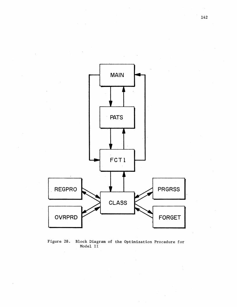
MAIN

PATS

FCTl

REG PRO PRGRSS

CLASS

OVRPRD FORGET

Figure 28. Block Diagram of the Optimization Procedure for Model II

142

143

of the planning horizon. The total number of units produced during

the planning horizon is assumed to be equal to the total demand during

the horizon.

The PATS routine is then called and the constant productivity model

is optimized. The results are then printed and input to CLASS through

a call to FCTl. This evaluates the performance of the constant pro­

ductivity model in situations where the dynamic productivity conditions

are present. The main routine then prints the results of this evaluation.

The optimum solution found for the constant productivity model is

used as the starting solution for the optimization process of the dy­

namic productivity model. This model is optimized (while the CLASS

routine is in effect) and the results are printed.

Subroutine FCTl increments the number of function evaluations,

receives the levels of the decision variables from PATS and directs

these levels to the cost function of the constant productivity model,

when this model is being optimized. The FCTl routine directs the

information received from PATS to the CLASS routine and receives back

the appropriate levels of the dependent variables. These levels,

together with the levels of the independent variables received from

PATS are then directed to a new (but equivalent) cost function with

the same cost coefficients. This new cost function does not include

the productivity factors; however, the function includes the dependent

variables. The appropriate levels of these variables are received

from CLASS.

Subroutine CLASS begins by detecting the period in which the

first change is made by PATS in the former levels of the decision

variables. This subroutine then incorporates the effect of manpower

144

change (through hiring and firing) into the condition of the experience

classes. The new conditions are then recorded in temporary locations.

The analysis of regular time and its effect on the experience

classes is then performed in this routine. At this step, the level of

the workforce on regular time and the level of the idle workforce (when

applicable) are computed for each period. After incorporating the

· effect of regular time work, a permanent status for each class is

then determined.

If the regular time work in any period does not satisfy the total

production scheduled for that period, the excess amount is then trans­

ferred to another part of the routine which incorporates the effect

of the overtime assignment on the conditions of the experience classes.

At this step, the levels of the overtime workforce and subcontracting

or the penalty factors of exceeding the maximum production capability

for an infeasible plan are generated (if subcontracting is not allowed).

After the incorporation of the effect of the overtime assignment on the

status of the classes, the permanent status for all classes in the

applicable periods is established.

Subroutine CLASS interfaces with four other routines: REGPRO, which

reports regular time production capability of members for any given pro­

ductivity measure OVRPRO, which reports overtime production capability of

members for any given productivity measure; PRGRSS, which reports the

applicable progress factor for any given cumulative units produced by

the firm; and FORGET, which reports the amount of decay in productivity

measure as a result of idle time, for any given productivity measure.

The Model II program listing is provided in Appendix F.

145

Remarks

The analysis and the optimization methodology developed in this

chapter have resulted in an integrated model which represents the work­

force body in every period of the planning horizon as a non-homogeneous

entity comprised of different classes of employees with their relevant

productivity rates. These productivity rates are determined on the

basis of the current improvement curve theories. The new model has a

number of advantages over the comparable model developed by Orrbeck

et al. because it incorporates more realistic assumptions while applying

the improvement curve analysis. Considering the solution approach

and the computational difficulties, there is also a considerable

difference between the two models.

Note that although the new model breaks the workforce body in each

period into a number of experience classes, the dimension of the

problem (number of independent variables) is still unchanged (twice the

number of periods). That is, the independent variables used in the

search technique are still the "total workforce" level and the production

rate for each period. Consequently, the new model has a considerable

advantage over the Orrbeck et al. model. In this latter model each

class in each period is represented by a new variable. These variables

are incorporated into the objective function and the constraints, there­

by resulting in a large model which (considering the available L.P.

packages) is computationally unattractive as compared with the perfor­

mance of the new model. Optimization of the new model on an IBM 370

system for a 10 period planning horizon (20 dimensions) requires a

computing time of a little over one minute. As experience shows, the

146

optimization of an equivalent model with structure proposed by Orrbeck

et al. would result in a large L.P. model (approximately 200 x 100)

which requires much more execution time and fast memory on the same

system (approximately 15 minutes).

The new model also has some advantages over all existing aggregate

planning models. For example, the length of overtime in this model

does not have to be considered as a constant fraction of the length

of the regular time for all periods throughout the planning horizon.

This quantity may be considered as a variable, thereby introducing

a new dimension to the optimization process. That is, three independent

variables can be assumed ·for every period. The optimization process

would then include the periodical length of overtime as a variable

which may assume different values within the prespecified boundaries.

In this case, the dimension of the problem will be three times larger

than the number of periods in the planning horizon.

Another general advantage of the new model is its capability of

producing additional information about the dependent variables in 'the

system. Workforce level on regular time, overtime and idle workforce

in each period along with production level related to each alternative

way of workforce utilization are some of these variables which can

help the analyst construct more realistic cost functions. In this

case, some approximations (such as quadratic approximation of overtime

cost) would be unnecessary. Also, note that the new model 9rovides the

size and experience level of each class in each period. Therefore, if

workers are to receive different wage incentives: relative to their

productivities, an even more realistic cost function can be constructed

and used in the new model.

CHAPTER VII

ANALYSIS OF RESULTS

Introduction

The objective of this chapter is to quantitatively evaluate the

impact of the new models developed in this research. The cost structure

selected for this purpose is the one developed for the original HMMS

paint factory problem which has frequently been utilized as a test

criterion by many researchers.

The basic problem encountered in this part of the research originates

from the fact that the existing actual data lack information regarding

learning productivity, since they are used to evaluate constant pro­

ductivity models. This may be the reason that Ebert and Orrbeck et al.

have used hypothetical data to demonstrate the performance of their

models.

The above problem has been overcome in the current research by

considering the fact that the constant productivity factor used in the

existing constant productivity models is actually the "average" pro­

ductivity rate determined on the basis of available accounting data.

Actually, it is possible to generate several learning curves that yield

a given average productivity over a range of cumulative output (from

the beginning through the end of the planning horizon). This can be

done by proper selection of sets of base unit cost, improvement slope,

and initial cumulative output quantity. For the paint factory problem

147

•

148

such improvement curves can be developed to provide a basis for rating

the relative performances of the new models. The evaluation algorithm

developed for this purpose is as follows:

Step 1. On the basis of the given overall average (constant) productivity and a range of cumulative output, generate an applicable improvement curve.

Step 2. Optimize the c-onstant productivity model. (Only the solution is -important at this step, the associated cost is not.)

Step 3. Using the dynamic productivity model, compute the total cost associated with the solution found in Step 2 (no optimization is performed at this step).

Step 4. Applying the improvement curve developed in St~p 1, optimize the dynamic productivity model.

Step 5. Compare the two costs found in Steps 3 and 4 (evaluate the two possibly different sets of solutions; the solution found in Step 3 is optimal only under constant productiv­ity assumption, and not necessarily optimal for the dynamic model).

Step 6. Repeat the above steps for different values of the model parameters.

Basically, the above algorithm evaluates the outcome of implement-

ing the solutions found by applying constant productivity models versus

the dynamic productivity models in situations where a constant productiv-

ity assumption does not hold.

Notice that the Ebert model can be substituted in Step 2 of the

above algorithm. The outcome of the evaluation in this case would be

the impact of disruptions generated by manpower transactions which are

not incorporated into the Ebert model.

Evaluation of Model I

As mentioned before, the actual data used in the paint factory

problem is chosen as the basis for testing the performance of the new

149

models. It was seen in Chapter IV, that the overall average productiv-

ity per employee in this problem is 5.67 units (gallons) per man

per month. Although thiscasedoes not ideally represent a long cycle

product situation (5.67 is rather large output quantity per man-month),

this case still seems to be closer to the long cycle product situation

rather than to a short cycle one (where the output per man-month is a

lot higher than 5.67). Thus, the paint factory data can suitably pro-

vide a basis for evaluation purposes regarding Model I.

Both the constant productivity and the Ebert models are compared

with the new model in this part of the analysis. The Ebert model is

used to show the impact of disruptions caused by the manpower trans-

actions.

Substituting the dynamic productivity factor as a variable in the

original cost structure of the paint factory model (shown in Chapter IV),

the new cost structure would have the following form:

s.t.

N Tc = L

t=l

. 2 {[340 Wt] + [64.3(Wt- Wt-1) ]

2 + (0.20(Pt - APtWt) + 51.2 Pt - 281 Wt]

+ (0.0825(It- 320) 2]}

t = 1, 2, ••• , N

where APt represents the average productivity per employee in period

t. The initial workforce and inventory levels in this model are 81 men

and 283 units, respectivel~ A planning horizon containing 10 periods .is

assumed in this analysis, thereby incorporating 20 independent (Wt and

Pt) and 10 dependent (APt) variables into the cost function. The

150

demand levels (Dt) for 10 consecutive months are given in the second

columns of the upper parts of the tables in the following pages. Work­

force levels and production rates are restricted to vary in the intervals

of 0 to 150 men and 0 to 1000 units, respectively.

Using the algorithm presented earlier in this chapter (Step 1) and

applying an improvement slope of 70% over the 10 month planning horizon,

a base unit cost of 16.55 man-months per unit is estimated. This esti­

mation is based on the assumption that the firm has produced 5,000 units

by the beginning of the planning horizon (cum0 = 5000). This improvement

curve is used in the Ebert and in the dynamic productivity models. The

minimum threshold level, TRSHL, for a significant manpower turnover and

the minimum unit cost difference ratio,EPSY for a significant compounded

disruption are .05 and 10%, respectively (see Appendix A).

Table IV shows the results of optimization of the average productiv­

ity model with original constant productivity level of 5.67 (on the basis

of which the improvement curve parameters are computed). This table

contains the same information contained in Table 2 of Chapter IV. The

results of optimization of the Ebert model are presented in Table V.

Notice that the monthly average productivites in this model increases

continuously. The magnitude of increments in the average productivity

in a month is proportional to the production rate in that month. Trans­

actions occuring in the workforce level do not affect these magnitudes.

It should be noted, that although the average of the monthly average

productivity levels in this model is very close to the overall average

productivity level in the equivalent constant productivity model, it

is not necessarily equal to this level. This is due to the fact that

the overall average productivity level is computed on the basis of the

Month

1 2 3 4 5 6 7 8 9

10

Mo.

1 2 3 4 5 6 7 8 9

10

TABLE IV

RESULTS OF OPTIMIZATION OF THE CONSTANT PRODUCTIVITY.MODEL CUM¢= 5,000

A. DECISIONS AND PROJECTIONS

Demand Work Production Inventory Force

430 77.7 470.5 303.5 447 74.3 444.1 300.6 440 70.9 417.1 277.7 316 67.7 381.7 343.4 397 65.1 376.2 322.5 375 62.7 363.8 311.4 292 60.7 348.9 368.3 458 59.0 359.4 269.7 400 57.4 329.3 199.0 350 56.1 272.2 121.2

B. COST ANALYSIS OF DECISIONS AND PROJECTIONS

Payroll Hiring & Overtime Inventory Firing

26,406.07 715.19 2,447.78 22.45 25,247.18 747.03 1,978.09 31.04 24,105.72 724.73 1,476.17 147.88 23,029.24 644.56 511.47 45.05 22,122.18 457.64 986.83 0.53 21,327.44 351.32 1,015.87 6.13 20,639.67 263.11 810.97 192.46 20,068.63 181.38 1,936.16 208.91 19,509.80 173.70 740.77 1,207.64 19,080.42 102.55 -1,408.60 3,259.04

151

Average Productivity

5.67 5.67 5.67 5.67 5.67 5.67 5.67 5.67 5.67 5.67

($)

Total

29,591.40 28.003.34 26,454.50 24,230.33 23,567.18 22,700.76 21,906.21 22,395.08 21;631.91 21,033.41

241,514.22

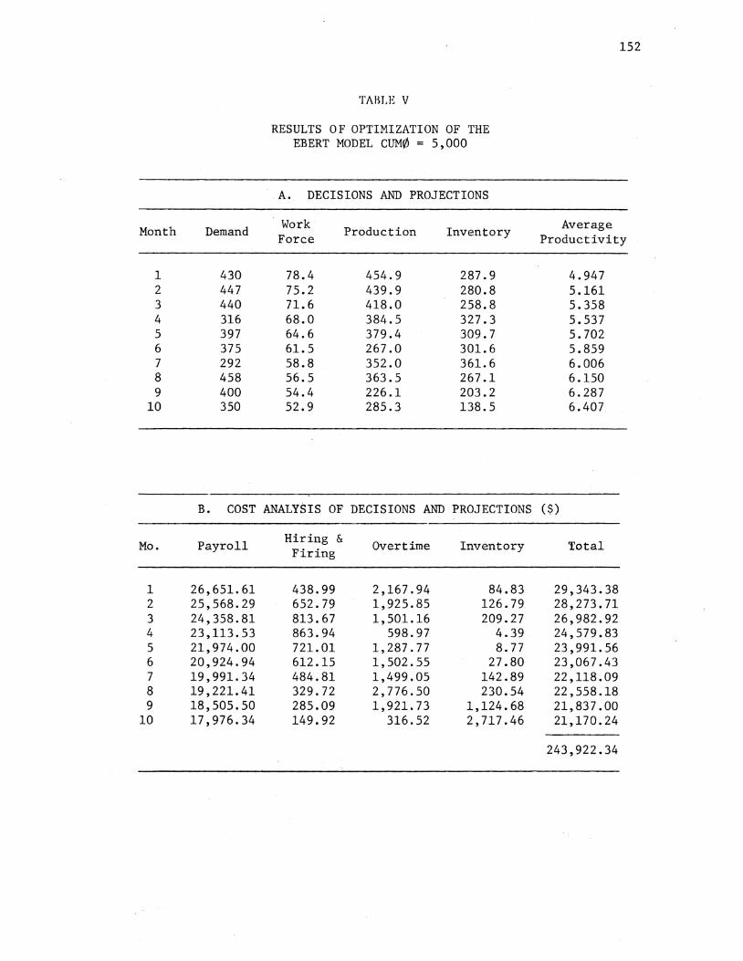
Month

1 2 3 4 5 6 7 8 9

10

Mo.

1 2 3 4 5 6 7 8 9

10

Demand

430 447 440 316 397 375 292 458 400 350

TABLE V

RESULTS OF OPTIMIZATION OF THE EBERT MODEL CUM0 = 5,000

A. DECISIONS AND PROJECTIONS

Work Production Inventory

Force

78.4 454.9 287.9 75.2 439.9 280.8 71.6 418.0 258.8 68.0 384.5 327.3 64.6 379.4 309.7 61.5 267.0 301.6 58.8 352.0 361.6 56.5 363.5 267.1 54.4 226.1 203.2 52.9 285.3 138.5

B. COST ANALYSIS OF DECISIONS AND PROJECTIONS

Payroll Hiring & Overtime Inventory Firing

26,651.61 438.99 2,167.94 84.83 25,568.29 652.79 1,925.85 126.79 24,358.81 813.67 1' 501.16 209.27 23,113.53 863.94 598.97 4.39 21,974.00 721.01 1,287.77 8.77 20,924.94 612.15 1,502.55 27.80 19' 991. 34 484.81 1,499.05 142.89 19' 221.41 329. 72 2' 776.50 230.54 18,505.50 285.09 1,921.73 1,124.68 17,976.34 149.92 316.52 2' 717.46

152

Average Productivity

4.947 5.161 5.358 5.537 5.702 5.859 6.006 6.150 6.287 6.407

($)

Total

29,343.38 28,273.71 26,982.92 24,579.83 23 '991. 56 23,067.43 22,118.09 22,558.18 21,837.00 21,170.24

243,922.34

153

monthly production rates. Evidently, the total production in the plan­

ning horizon could differ from the total demands in the horizon. This

is due to the existance of the initial and ending inventory levels which

are allowed in these models. Of course, the overall average productivity

cannot be computed on the basis of the total production, because the

monthly production rates are decision variables which are notknownprior

to the optimization process. ·However, the monthly demands are assumed

to be known prior to determination of these variables; therefore, they

are used to estimate the overall average productivity.

As mentioned earlier in this chapter, the cost analysis of the

optimization results of the constant productivity and the Ebert models

is not relevant for the current purpose; however, the projected decision

variables are: the actual cost of implementing these decisions in

situations where disruption effects exist is, of course, larger than

what is indicated by the models. Tables VI and VII shown the results of

implementing these decisions in such. a situation. To compute the entries

in these tables, the projected decisions by the constant productivity and

the Ebert models are used to evaluate the objective function of the

dynamic productivity model. The actual average productivities (versus

the projected ones) are computed using the PROCTV routine. No optimiza­

tion is performed at this stage.

The entries in the columns under INDEX indicate the occurance of

significant disruption as a result of manpower transactions. If such

disruption occurs at the beginning of a given period, the value of INDEX

for that period is one; otherwise, it is zero. The entries in the

columns under ICHK for a given period indicate the existance of a

significant disruption effect carried over from previous period(s). If

154

such a case occurs, the value of ICHK is one; otherwise, it is zero.

If both INDEX and ICHK are one in a period, this indicates the occurrence

of a compounded disruption.

Notice that implementation of the constant productivity model

(Table VI) does not incorporate any disruption. However, implementation

of the Ebert model incorporates one significant disruption at the begin­

ning of the fourth period (TableVII). This disruption is caused by a

manpower reduction of size 3.6 which is the largest change throughout the

planning horizon. Also notice the effect or this change in the productiv­

ity level for this period; while the Ebert model indicates a productivity

level of 5.537 in this period (Table V), the actual productivity is

5.205 (as indicated by the new model) the difference being due to the

disruption occurring at this period.

Since the average productivity level is constant in the constant

productivity model, the projected workforce level is relatively smoother

in this model. However, since the average productivites are continu­

ously increasing in the Ebert model, the projected manpower level is

continuously decreasing in this model. This is why the implementation

of the constant productivity model does not incorporate any disruption,

but implementation of the Ebert model does.

The cost analysis given in Tables VI and VII are important and can

be compared with the cost of implementing the dynamic productivity model.

The results of optimization and implementation of the dynamic pro­

ductivity model are given in Table VIII. Notice that this model projects

decisions which indicate the lowest total cost of implementation. Note

that the Ebert model performs better than the constant productivity

model. This is simply because of the better estimation of the actual

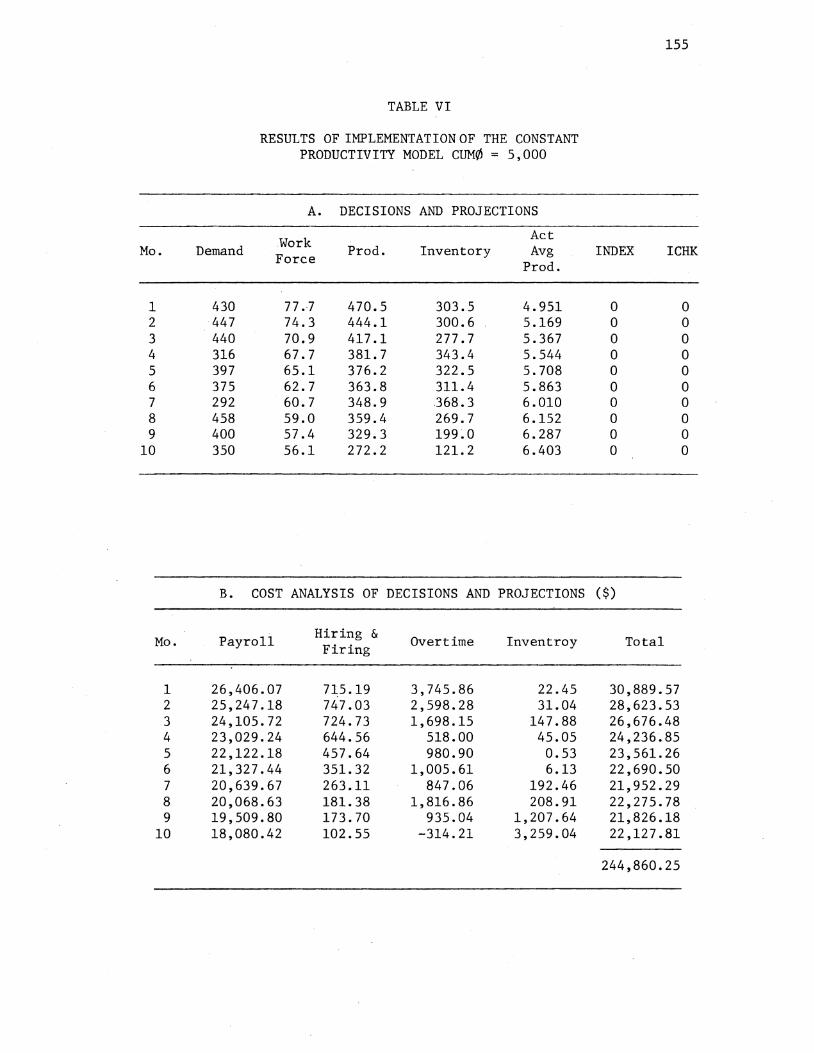
Mo.

1 2 3 4 5 6 7 8 9

10

Mo.

1 2 3 4 5 6 7 8 9

10

TABLE VI

RESULTS OF IMPLEMENTATION OF THE CONSTANT PRODUCTIVITY MODEL CUM0 = 5,000

A. DECISIONS AND PROJECTIONS

Work Act Demand Force Prod. Inventory Avg

Prod.

430 77.7 470.5 303.5 4.951 447 74.3 444.1 300.6 5.169 440 70.9 417.1 277.7 5.367 316 67.7 381.7 343.4 5.544 397 65.1 376.2 322.5 5.708 375 62.7 363.8 311.4 5.863 292 60.7 348.9 .368. 3 6.010 458 59.0 359.4 269.7 6.152 400 57.4 329.3 199~0 6.287 350 56.1 272.2 121.2 6.403

B. COST ANALYSIS OF DECISIONS AND PROJECTIONS

Payroll Hiring & Overtime Invent roy Firing

26,406.07 715.19 3,745.86 22.45 25,247.18 747.03 2,598.28 31.04 24,105.72 724.73 1,698.15 147.88 23,029.24 644.56 518.00 45.05 22,122.18 457.64 980.90 0.53 21,327.44 351.32 1,005.61 6.13 20,639.67 263.11 847.06 192.46 20,068.63 181.38 1,816.86 208.91 19,509.80 173.70 935.04 1,207.64 18,080.42 102.55 -314.21 3,259.04

155

INDEX ICHK

0 0 0 0 0 0 0 0 0 0 0 0 0 0 0 0 0 0 0 0

($)

Total

30,889.57 28,623.53 26,676.48 24 '236 •. 85 23,561.26 22,690.50 21,952.29 22,275.78 21,826.18 22,127.81

244,860.25

Mo.

1 2 3 4 5 6 7 8 9

10

Mo.

1 2 3 4 5 6 7 8 9

10

TABLE VII

RESULTS OF IMPLEMENTATION OF THE EBERT MODEL CUM¢ = 5,000

A. DECISIONS AND PROJECTIONS

Work Act Demand Force Prod. Inventory Avg

Prod.

430 78.4 454.9 287.9 4.947 447 75.2 439.9 280.8 5.161 440 71.6 418.0 258.8 5.358 316 68.0 384.5 327.3 5.205 397 64.6 379.4 309.7 5.702 375 61.5 367.0 301.6 5.859 292 58.8 352.0 361.6 6.006 458 56.5 363.5 267.1 6.150 400 54.4 366.1 203.2 6.287 350 52.9 285.3 138.5 6.407

B. COST ANALYSIS OF DECISIONS AND PROJECTIONS

Payroll Hiring & Overtime Inventory Firing

26,651.61 438.99 2,167.94 84.83 25,568.29 652.79 1,925.85 126.79 24,358.81 813.67 1, 501.16 309.27 23,112.53 863.94 774.21 4.39 21,974.00 721.01 1,287.77 8. 77 20,924.94 612.15 1,502.55 27.80 19,991.34 484.81 1,499.05 142.89 19' 221.41 329.72 2' 776.50 230.54 18,505.50 285.08 1, 921.73 1,124.68 17,986.34 149.92 316.52 2,717.46

156

INDEX ICHK

0 0 0 0 0 0 1 0 0 0 0 0 0 0 0 0 0 0 0 0

($)

Total

29,343.38 28,273.71 26,982.92 24,755.07 23,991.56 23,067.43 22,118.09 22,558.18 21,837.00 21,170.24

244,097.57

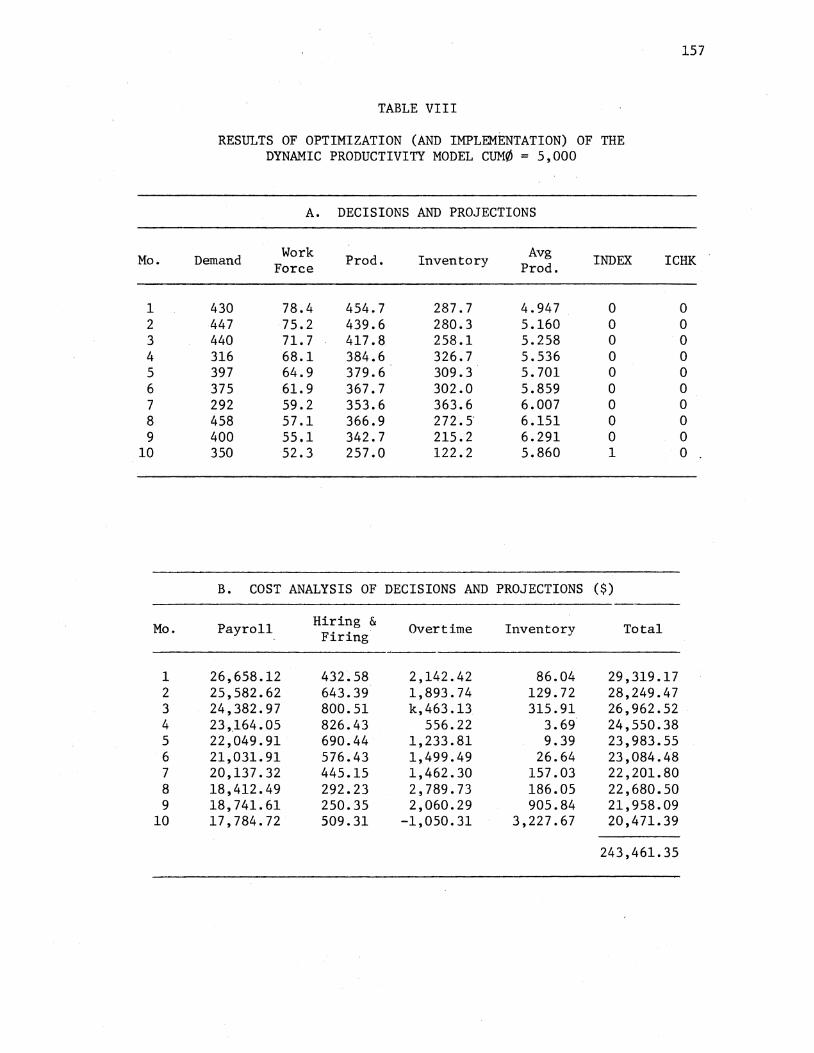
Mo.

1 2 3 4 5 6 7 8 9

10

Mo.

1 2 3 4 5 6 7 8 9

10

TABLE VIII

RESULTS OF OPTIMIZATION (AND IMPLEMENTATION) OF THE DYNAMIC PRODUCTIVITY MODEL CUM¢ = 5,000

A. DECISIONS AND PROJECTIONS

157

Demand Work Prod. Inventory Avg INDEX ICHK Force Prod.

430 78.4 454.7 287.7 4.947 0 0 447 75.2 439.6 280.3 5.160 0 0 440 71.7 417.8 258.1 5.258 0 0 316 68.1 384.6 326.7 5.536 0 0 397 64.9 379.6 309.3 5.701 0 0 375 61.9 367.7 302.0 5.859 0 0 292 59.2 353.6 363.6 6.007 0 0 458 57.1 366.9 272. 5· 6.151 0 0 400 55.1 342.7 215.2 6.291 0 0 350 52.3 257.0 122.2 5.860 1 0

B. COST ANALYSIS OF DECISIONS AND PROJECTIONS ($)

Payroll Hiring & Overtime Inventory Total Firing

26,658.12 432.58 2,142.42 86.04 29,319.17 25,582.62 643.39 1,893.74 129.72 28,249.47 24,382.97 800.51 k,463.13 315.91 26,962.52 23,164.05 826.43 556.22 3.69 24,550.38 22,049.91 690.44 1,233.81 9.39 23,983.55 21,031.91 576.43 1,499.49 26.64 23,084.48 20,137.32 445.15 1,462.30 157.03 22 '201. 80 18,412.49 292.23 2,789.73 186.05 22,680.50 18,741.61 250.35 2,060.29 905.84 21,958.09 17' 784.72 509.31 -1,050.31 3,227.67 20,471.39

243,461.35

158

average productivity levels performed by the former model.

As this part of analysis indicates, there is no major cost advan­

tage of one model over the other (.57% better performance for the

dynamic productivity model over the constant productivity model and

.26% over the Ebert model). This is due to the particular level of

cum0 (selected on purpose to show the effect).

To clarify the above point, note that improvement curves approach

a horizontal line as the cumulative unit number increases; therefore,

average productivities indicated by the Ebert model become closer to

the overall average productivity computed for a range of large cumula­

tive output quantities. Thus, for these ranges the Ebert model would

approximately duplicate the results of the constant productivity model,

resulting in a low relative performance. The best relative performance

of the Ebert model over the constant productivity model is expected in

the early stages of production (low values of cum0 ). On the other hand,

the performance of the dynamic productivity model indicates that the

disruption effects are insignificant in the early stages of production.

This is expectable since in the early stages productivities of the old

and new workers do not differ much. A manpower addition, for example,

does not degrade the overall productivity, significantly. However in the

larger production sequences,due to the larger difference between the

productivity levels of the old and the new employees, an increase in

the manpower level would have a greater impact on the overall average

productivity. Therefore, in the early stages of production the per­

formance of the dynamic productivity model is close to the performance

of the Ebert model (both models performing better than the constant

productivity model). As the production sequence becomes larger, the

159

relative performances of the Ebert and the dynamic productivity model

over the constant productivity model become smaller. This decreasing

pattern in the relative performances continues until the effect·of

manpower disruptions starts to become significant (due to the larger

production sequences). From this point on, the relative performance

of the dynamic productivity model over the other two models follows an

increasing pattern.

Tables IX through XIX show the results of implementing the three

models for initial cumulative units of 0, 10,000, 25,000, and 50,000

(the cost analysis of the optimization results of the constant productiv-

ity and the Ebert models are not included in these tables, because as

mentioned before, these analyses are not relevant for the current purpose).

In these tables notice that:

1. At cum0 =0 the dynamic productivity model performs exactly similar to the Ebert model (Table X ) .

2. The deviations of the average productivities projected by the Ebert model from the overall average productivity, projected by the constant productivity model, become smaller as cum0

increases.

3. The relative performance (on the basis of the total cost) of Ebert model over the constant productivity model decays as cum0 increases.

4. More significant disruptions occur as cumo increases.

5. The deviations of the average productivities projected by the dynamic productivity model from the average productivit~es projected by the other two models increase significantly as cum0 increases.

6. The relative performance of the dynamic productivity model over the other two models improves as cum0 increases.

Figures 29 through 32 demonstrate those conditions mentioned in

(1), (2) and (5) above. Table XX contains a summary analysis. of the

relative performances. Figure 33 depicts the pattern of the changes in

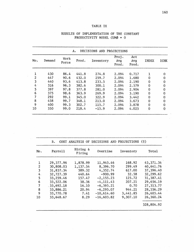
Mo.

1 2 3 4 5 6 7 8 9

10

Mo.

1 2 3 4 5 6 7 8 9

10

TABLE IX

RESULTS OF IMPLEMENTATION OF THE CONSTANT PRODUCTIVITY MODEL CUM0 = 0

A. DECISIONS AND PROJECTIONS

Work Proj. Act Demand Force Prod. Inventory. Avg Avg

Prod. Prod.

430 86.4 441.8 274.8 2.094 o. 717 447 90.6 432.0 259.7 2.094 1.680 440 93.6 413.8 233.5 2.094 2.190 316 96.3 382.6 300.1 2.094 2.579 397 97.8 377.8 281.0 2.094 2.904 375 98.6 363.9 269.9 2.094 3.190 292 99.1 345.0 322.9 2.094 3.442 458 99.7 348.1 213.0 2.094 3.673 400 99.3 302.7 115.7 2.094 3.878 350 99.0 218.4 -15.9 2.094 4.025

B. COST ANALYSIS OF DECISIONS AND PROJECTIONS

Payroll Hiring & Overtime Inventory Firing

29,377.96 1,878.99 11,945.46 168.92 30,808.03 1,137.54 8,396.70 299.49 31,837.34 589.32 4,352.74 617.00 32,727.39 440.64 -900.99 32.58 33,259.46 157.47 -2,155.23 125.72 33,522.06 38.36 -4,111.43 207.21

.33,692.18 16.10 -6,395.21 0.70 33,886.21 20.94 -6,295.07 944.21 33,770.78 7.41 -10,614.60 3,441.85 33,648.67 8.29 -16,603.82 9,307.10

160

INDEX ICHK

1 0 0 0 0 0 0 0 0 0 0 0 0 0 0 0 0 0 0 0

($)

Total

43,371.34 40' 641.76 37,396.40 32,299.62 31,387.41 29,656.19 27,313.77 28,556.29 26,605.44 26,360.24

328,804.92

Mo.

1 2 3 4 5 6 7 8 9

10

Mo.

1 2 3 4 5 6 7 8 9

10

TABLE X

RESULTS OF OPTIMIZATION (AND IMPLEMENTATION) OF THE EBERT AND THE DYNAMIC PRODUCTIVITY MODELS CUM¢ = 0

A. DECISIONS AND PROJECTIONS

161

Demand Work Prod. Inventory Avg INDEX ICHK Force Prod.

430 84.1 416.7 349.7 0.698 0 0 447 86.9 426.8 229.5 1.642 0 0 440 88.7 412.0 201.5 2.156 0 0 316 89.5 383.9 269.4 2.551 0 0 397 89.5 381.9 254.3 2.880 0 0 375 88.9 371.5 250.8 3.173 0 0 292 87.8 357.9 316.7 3.434 0 0 458 86.6 370.0 228.7 3.676 0 0 400 85.2 344.9 173.6 3.900 0 0 350 84.2 297.4 120.9 4.092 0 0

B. COST ANALYSIS OF DECISIONS AND PROJECTIONS ($)

Payroll Hiring & Overtime Inventory Total Firing

28,599.20 624.04 23,333.75 407.61 53,964.60 28,550.70 503.58 13,567.30 675.82 44,297.41 30,164.71 209.70 5,907.27 1,158.31 37,439.99 30,431.46 39.58 -656.85 211.41 30,025.60 30,434.02 0.00 -2,521.15 356.35 28,269.23 30,212.87 27.21 -4,342.49 394.90 26,292.49 29,847.56 74.23 -5,708.97 0. 91 24,213.73 29,432.74 94.71 -4,842.77 687.68 25,373.37 28,971.41 118.38 -6,255.48 1,769.00 24,603.31 28,615.26 70.56 -7,981.78 3,268.91 23,972.94

317,452.67

Mo.

1 2 3 4 5 6 7 8 9

10

Mo.

1 2 3 4 5 6 7 8 9

10

TABLE XI

RESULTS OF IMPLEMENTATION OF THE CONSTANT PRODUCTIVITY MODEL CUM¢ = 10,000

A. DECISIONS AND PROJECTIONS

Work Proj. Act Demand Force Prod. Inventory Avg Avg

Prod. Prod.

430 71.9 502.9 335.9 7.670 6.038 447 64.3 451.7 340.6 7.670 7.172 440 58.3 413.6 314.3 7.670 6.026 316 53.4 374.2 372.5 7.670 5. 977 397 49.9 368.8 344.3 7.670 6.064 375 47.2 357.9 327.2 7.670 6.168 292 45.0 344.2 379.4 7.670 6.755 458 43.3 355.6 277 .o 7.670 7.019 400 41.5 324.0 201.0 7.670 7.222 350 40.0 263.5 114.5 7.670 7.375

B. COST ANALYSIS OF DECISIONS AND PROJECTIONS

Payroll Hiring & Overtime Inventory Firing

24,432.25 5,372.10 6,510.09 20.91 21,871.78 3,646.65 5,650.17 35.16 19,805.27 2,375.35 5,593.02 2. 72 18,163.59 1,499.10 4,751.26 227.24 16,965.79 798.04 5,740.33 48.79 16,026.58 480.27 5,969.54 4.31 15,294.90 305.97 5,304.64 291.01 14,716.01 186.40 6,580.97 152.62 14,101.31 210.17 5,053.78 1,168.64 13,594.87 142.67 2,451.68 3,485.48

162

INDEX ICHK

1 1 1 1 1 1 1 1 1 1 1 1 0 1 0 1 0 1 0 1

($)

Total

36,335.36 31,203.76 27,776.36 24.641.19 23,552.94 22,490.70 21,196.53 21,636.00 20,533.91 19,674.70

249,041.43

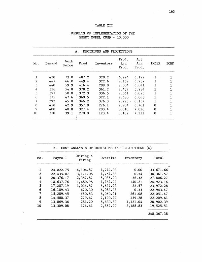
Mo.

1 2 3 4 5 6 7 8 9

10

Mo.

1 2 3 4 5 6 7 8 9

10

TABLE XII

RESULTS OF IMPLEMENTATION OF THE EBERT MODEL CUM¢ = 10,000

A. DECISIONS AND PROJECTIONS

Work Proj. Act Demand Force Prod. Inventory Avg Avg

Prod. Prod.

430 73.0 487.2 320.2 6.994 6.129 447 66.0 449~4 322.6 7.157 6.237 440 59.9 416.4 299.0 7.304 6.041 316 54.8 378.2 361.2 7.437 5.984 397 50.8 372.3 336.5 7.561 6:023 375 47.6 360.5 322.1 7.680 6.083 292 45.0 346.2 376.3 7. 793 . 6.157 458 42.9 357.8 276.1 7.904 6.761 400 40.8 327.4 203.4 8.010 7.026 350 39.1 270.0 123.4 8.102 7. 211

B. COST ANALYSIS OF DECISIONS AND PROJECTIONS

Payroll Hiring & Overtime Inventory Firing

24,822.75 4,106.87 4,742.03 0.00 22,435.07 3, 171.08 4,754.88 0.54 20,376.17 2,357.87 5,035.90 36.32 18,637.76 1,680.98 4,464.22 140.21 17,287.19 1,014.57 5,647.94 22.57 16,189.43 670.30 6,083.38 0.35 15,289.45 450.53 6,050.41 261.08 14,580.37 279.67 7,190.29 159.28 13,869.36 281.20 5,630.80 1' 121.04 13,309.08 174.61 2,852.99 3,188.83

163

INDEX ICHK

1 1 1 1 1 1 1 1 1 1 1 1 1 1 0 1 0 1 0 1

($)

Total

33,671.66 30,361.57 27,806.27 24,923.16 23,972.28 22,943.47 22,051.47 22,209.61 20,902.39 19,525.51

248,367.38

Mo.

1 2 3 4 5 6 7 8 9

10

Mo.

1 2 3 4 5 6 7 8 9

10

TABLE XIII

RESULTS OF OPTIMIZATION (AND IMPLEMENTATION) OF THE DYNAMIC PRODUCTIVITY MODEL CUM¢ = 10,000

A. DECISIONS AND PROJECTIONS

164

Demand Work Prod. Inventory Avg INDEX ICHX Force Prod.

430 74.8 482.1 ·315.1 6. 301 1 0 447 69.1 452.8 320.8 6.414 1 0 440 63.8 423.3 304.1 6.494 1 1 316 58.6 368.2 356.3 6.246 1 1 397 54.1 350.8 310.1 6.147 1 1 375 51.4 365.0 300.1 6.863 0 1 292 48.9 353.2 361.3 7.137 0 1 458 46.8 363.9 267.2 7.343 0 1 400 44.6 333.8 201.0 7.514 0 1 350 43.0 278.8 129.9 7.650 0 1

B. COST AN4LYSIS OF DECISIONS AND PROJECTIONS ($)

Payroll Hiring & Overtime Inventory Total Firing

25,433.55 2,468.06 3,684.13 2.01 31,487.75 23,504.36 2,070.15 3,773.86 0.06 29,348.43 21,690.38 1,830.30 3,760.75 20.87 27,302.29 19,927.43 1,728.74 2,383.15 108.67 24,147.99 18,400.41 1,297.01 2,817.83 8.13 22,523.38 17,480.71 470.49 . 4,270.56 32.74 22,254.50 16,628.63 403.85 4,346.54 140.87 21,519.88 15,901.07 294.44 5,573.33 229.89 21,998.73 15,173.72 294.26 4,551.68 1,167.55 21,187.21 14,613.89 174.32 2,697.87 2,982.21 20,468.30

242,338.47

Mo.

1 2 3 4 5 6 7 8 9

10

Mo.

1 2 3 4 5 6 7 8 9

10

TABLE XIV

RESULTS OF IMPLEMENTATION OF THE CONSTANT PRODUCTIVITY MODEL CUM~ = 25,000

A. DECISIONS AND PROJECTIONS

Work Proj. Act Demand Force Prod. Inventory Avg Avg

Prod. Prod.

430 62.2 571.8 404.8 11.57 5 7.376 447 49.1 455.6 413.4 11.575 7.276 440 40.6 395.3 268.6 11.575 6.792 316 35.2 352.7 405.4 11.57 5 6.670 397 32.2 353.3 361.6 11.575 6.984 375 30.3 349.0 335.6 11.57 5 7.325 292 29.0 340.1 383.7 11.575 8.288

- 458 27.9 354.4 280.0 11.575 8.731 400 26.3 218.4 198.4 11.575 7.921 350 24.5 248.0 96.4 11.575 7.474

B. COST ANALYSIS OF DECISIONS AND PROJECTIONS

Payroll Hiring & Overtime Inventory Firing

21,135.29 22,816.69 . 14,371.92 592.78 16,695.46 10,964.42 11,272.21 719.12 13,792.03 4,688.93 11,707.75 195.12 11,953.65 1,879.86 10,976.39 601.25 10,935.04 577.13 12,359.42 142.96 10,305.21 220.65 12,575.73 20.11

9,853.95 113.26 11,262.39 334.56 9,502.32 68.78 12,726.20 131.68 8,928.80 182.96 11,355.86 1,219.70 8,335.07 196.08 6,647.61 4,124.52

165

INDEX ICHK

1 1 1 1 1 1 1 1 1 1 1 1 0 1 0 1 1 1 1 1

($)

Total

58,916.68 39,651.20 30.383.84 25,411.15 24,014.54 23,121.69 21,564.17 22,428.98 21,687.32 19,303.28

286,482.85

Mo.

1 2 3 4 5 6 7 8 9

10

Mo.

1 2 3 4 5 6 7 8 9

10

TABLE XV

RESULTS OF IMPLEMENTATION OF THE EBERT MODEL CUM¢ = 25,000

A .. DECISIONS AND PROJECTIONS

Work Proj. Act Demand Force Prod. Inventory Avg Avg

Prod. Prod.

430 62.9 561.1 394.1 11.134 7.450 447 50.1 456.3 403.5 11.248 7.454 440 41.5 398.7 362.2 11.344 6.846 316 35.8 355.8 402.0 11.428 6.679 397 32.6 ! 355.1 360.1 11.506 6.933 375 30.5 349.9 335.0 11.583 7.222 292 28.9 340.5 282.6 11.658 7.460 458 27.7 354.8 280.4 11.7 34 8.349 400 25.9 319.0 199.4 11.806 7.619 350 24.1 249.4 98.8 11.867. 7. 225 .

B. COST ANALYSIS OF DECISIONS AND PROJECTIONS

Payroll Hiring & Overtime Inventory Firing

21,386.38 21,062.74 12,767.28 453.46 17,027.49 10,568.30 10,669.46 574.76 14,094.58 4,774.87 11,401.18 146.79 12,183.20 2,038.50 10,859.85 554.21 11,073.90 684.46 12,376.01 132.68 10,359.17 284.14 12,728.63 18.65

9,837.07 151.62 12,413.87 333.23 9 ,431. 35 91.56 13,407.38 129.61 8,817.68 209.47 11,997.40 1,199.85 8,199.44 212.60 7,118.29 4,038.33

166

INDEX ICHK

1 1 1 1 1 1 1 1 1 1 1 1 1 1 0 1 1 1 1 1

($)

Total

55,669.85 38~840.00 30,420.42 26,635.76 24,267.04 23,390.59 22,735.79 23,059.90 22,224.40 19,568.66

. 285,812.41

Mo.

1 2 3 4 5 6 7 8 9

10

Mo.

1 2 3 4 5 6 7 8 9

10

TABLE XVI

RESULTS OF IMPLEMENTATION OF THE DYNAMIC PRODUCTIVITY MODEL CUM~ = 25,000

A. DECISIONS AND PROJECTIONS

Demand Work Prod. Inventory Avg Force Prod.

430 69.1 518.2 351.2 8-.321 447 59.7 460.0 364.2 8.401 440 53.2 404.3 328.5 7.970 316 48.1 357.1 369.6 7. 711 397 44.8 361.1 333.7 7.857 375 41.8 339.3 297.9 7.785 292 39.7 356.5 362.5 8.876 458 37.9 374.8 279.3 9.323 400 36.0 351.5 230.8 9.644 350 32.6 207.7 88.5 7.534

B. COST ANALYSIS OF DECISIONS AND PROJECTIONS

Payroll Hiring & Overtime Inventory Firing

23,506.68 9,048.55 7,757.18 80.44 20,304.08 5,705.02 7,116.98 161.01 18,073.53 2,767.45 5,837.42 5.92 16,358.77 1,635.52 4,804.37 203.10 15,228.95 710.03 5,916.83 15.44 14,206.79 581.15 5,667.29 40.18 13,497.54 280.59 7,105.29 148.74 12,800.25 197.77 8,617.19 136.88 12,255.48 231.24 7,872.21 656.56 11,099.36 743.46 1,752.91 4,422.16

167

INDEX ICHX

1 1 1 1 1 1 1 1 1 1 1 1 0 1 0 1 0 1 1 1

($)

Total

40.392.85 33,287.09 26,684.31 23,001.76 21,871.24 20,495.41 21,029.15 21,852.09 21,015.49 18,017.89

247,647.29

Mo.

1 2 3 4 5 6 7 8 9

10

Mo.

1 2 3 4 5 6 7 8 9

10

TABLE XVli

RESULTS OF IMPLEMENTATION OF THE CONSTANT PRODUCTIVITY MODEL CUM~ = 50,000

A. DECISIONS AND PROJECTIONS

Work Proj. Act Demand Force Prod. Inventory Avg Avg

Prod. Prod.

430 53.3 646.0 479.0 16.070 7.839 447 36.7 444.0 475.9 16.070 7.436 440 27.8 365.0 401.0 16.070 6.586 316 23.4 327.7 412.7 16.070 6.695 397 21.8 341.1 356.8 16.070 7.654 375 21.2 346.4 328.2 16.070 9.091 292 20.8 342.9 379.1 16.070 9.801 458 20.4 360.6 281.7 16.070 10.343 400 18.7 318.6 200.4 16.070 8.763 350 16.7 236.4 86.4 16.070 7.529

B. COST ANALYSIS OF DECISIONS AND PROJECTIONS

Payroll Hiring & Overtime Inventory Firing

18,134.38 49,207.09 28,471.61 2,085.05 12,472.98 17,827.95 18,282.65 2,006.42

9 ,441. 21 5,112.64 17,518.79 540.74 7,945.93 1,243.65 16,079.77 708.87 7,419.36 154.23 17,389.80 111.57 7,211.87 23.95 16,496.06 5.57 7,065.68 11.89 15,596.20 288.55 6,923.17 11.30 17,239.01 120.88 6,369.73 170.37 15,821.66 1,180.94 5,673.64 269.52 9,866.69 4,488.84

168

INDEX ICHK

1 1 1 1 1 1 1 1 1 1 0 1 0 1 0 1 1 1 1 1

($)

Total

97,898.13 50,589.99 32,613.38 25,978.22 25,074.95 23,737.44 22,962.31 24,294.36 23,542.69 20,298.69

346,990.17

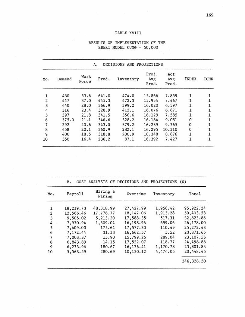
Mo.

1 2 3 4 5 6 7 8 9

10

Mo.

1 2 3 4 5 6 7 8 9

10

TABLE XVIII

RESULTS OF IMPLEMENTATION OF THE EBERT MODEL CUM¢ = 50,000

A. DECISIONS AND PROJECTIONS

Work Proj. Act Demand Force Prod. Inventory Avg Avg

Prod. Prod.

430 53.6 641.0 474.0 15.866 7.859 447 37.0 445.3 472.3 15.954 7.467 440 28.0 366.9 :399.2 16.020 6.597 316 23.4 328.9 412.1 16.076 6.671 397 21.8 341.5 356.6 16.129 7.585 375.0 21.1 346.6 328.2 16.184 9.051 292 20.6 343.0 379.2 16.239 9.765 458 20.1 360.9 282.1 16.295 10.310 400 18.5 318.8 200.9 16.348 8.676 350 16.4 236.2 87.1 16.392 7.427

B. COST ANALYSIS OF DECISIONS AND PROJECTIONS

Payroll Hiring & Overtime Inventory Firing

18,219.73 48,318.99 27,427.99 1,956.42 12,566.46 17.776.77 18,147.06 1,913.28 9,505.02 5,213.20 17,588.35 517.31 7,970.94 1,309.04 16,198.96 699.06 7,409.00 175.64 17,577.30 110.49 7,172.44 31.13 16,662.57 5.52 7,003.37 15.90 15,799.25 289.04 6,843.89 14.15 17,522.07 118.77 6,273.96 180.67 16,176.41 1,170.78 5,563.59 280.69 10,130.12 4,474.05

169

INDEX ICHK

1 1 1 1 1 1 1 1 1 1 0 1 0 1 0 1 1 1 1 1

($)

Total

95,922.24 50,403.58 32,823.88 26,178.00 25,272.43 23,871.65 23,107.56 24,498.88 23,801.83 20,448.45

346,328.50

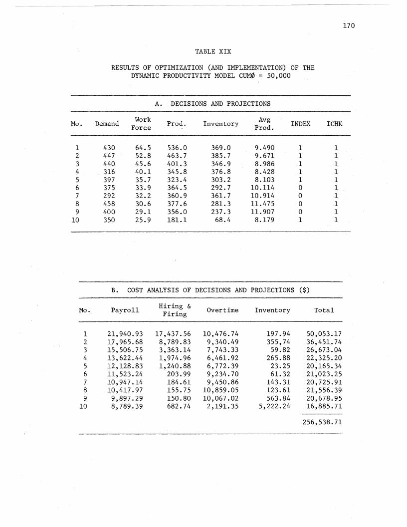
Mo.

1 2 3 4 5 6 7 8 9

10

Mo.

1 2 3 4 5 6 7 8 9

10

TABLE XIX

RESULTS OF OPTIMIZATION (AND IMPLEMENTATION) OF THE DYNAMIC PRODUCTIVITY MODEL CUM¢ = 50,000

A. DECISIONS AND PROJECTIONS

Demand Work Prod. Inventory Avg INDEX ICHK Force Prod.

430 64.5 536.0 369.0 9.490 1 1 447 52.8 463.7 385.7 9. 671 1 1 440 45.6 401.3 346.9 8.986 1 1 316 40.1 345.8 376.8 8.428 1 1 397 35.7 323.4 303.2 8.103 1 1 375 33.9 364.5 292.7 10.114 0 1 292 32.2 360.9 361.7 10.914 0 1 458 30.6 377.6 281.3 11.475 0 1 400 29.1 356.0 237.3 11.907 0 1 350 25.9 181.1 68.4 8.179 1 1

B. COST ANALYSIS OF DECISIONS AND PROJECTIONS ($)

Payroll Hiring & Overtime Inventory Total Firing

21,940.93 17,437.56 10,476.74 197.94 50,053.17 17,965.68 8,789.83 9,340.49 355,74 36,451.74 15,506.75 3,363.14 7,743.33 59.82 26,673.04 13,622.44 1,974.96 6,461.92 265.88 22,325.20 12,128.83 1,240.88 6,772.39 23.25 20,165.34 11,523.24 203.99 9,234.70 61.32 21,023.25 10,947.14 184.61 9,450.86 143.31 20,725.91 10,417.97 155.75 10,859.05 123.61 21,556.39

9,897.29 150.80 10,067.02 563.84 20,678.95 8,789.39 682.74 2,191.35 5,222.24 16,885.71

256,538.71

170

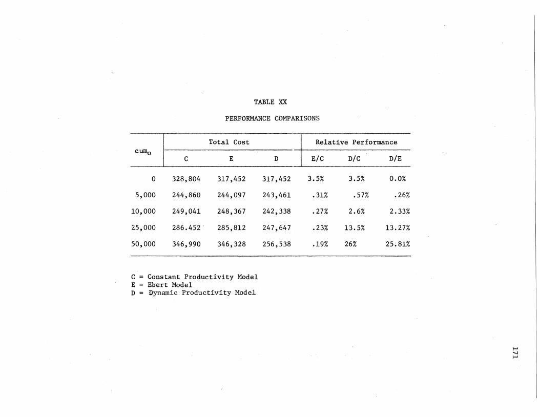
TABLE XX

PERFORMANCE COMPARISONS

Total Cost cum0

c E

0 328,804 317,452

5,000 244,860 244,097

10,000 249,041 248,367

25,000 286.452 285,812

50,000 346,990 346,328

C = Constant Productivity Model E = Ebert Moc:lel D = Dynamic Productivity Model

D

317,452

243,461

242,338

247,647

256,538

Relative Performance

E/C D/C D/E

3.5% 3.5% 0.0%

.31% .57% .26%

.27% 2.6% 2.33%

.23% 13.5% 13.27%

.19% 26% 25.81%

6.6 -----Constant Productivity Model

6.4 ----- Ebert Model

Dynamic Productivity Model

6.2

>. .....

'" 6.0 ~ ..... tl =' "' 5.8 0 .. p.,

GJ co 5.6 CIS .. GJ

~ 5.4

5.2

5.0

1 2 3 4 5 6 7 8 9 10.

Production Periods

Figure 29. Average Productivity Patterns Over 10 Month Plannig Horizon (cum =5000)

0

172

8.2

8.0

7.8

7.6

6.6

6.4·

6.2

0

/

,..-_/

/ /

.,..., ..., ..... ,.--

------------ ~---- ------

, ,,

1

./

2

/~ /

/

3

r"' /

4

,./' /

5

,

-- -- -- Constant Productivity Model

- -- - - Ebert Model

------ Dyanmic Productivity Model

6 7 8 9 10

Production Periods

Figure 30, Average Productivity Patterns Over 10 Month Planning Horizon-{cum0=10,000)

173

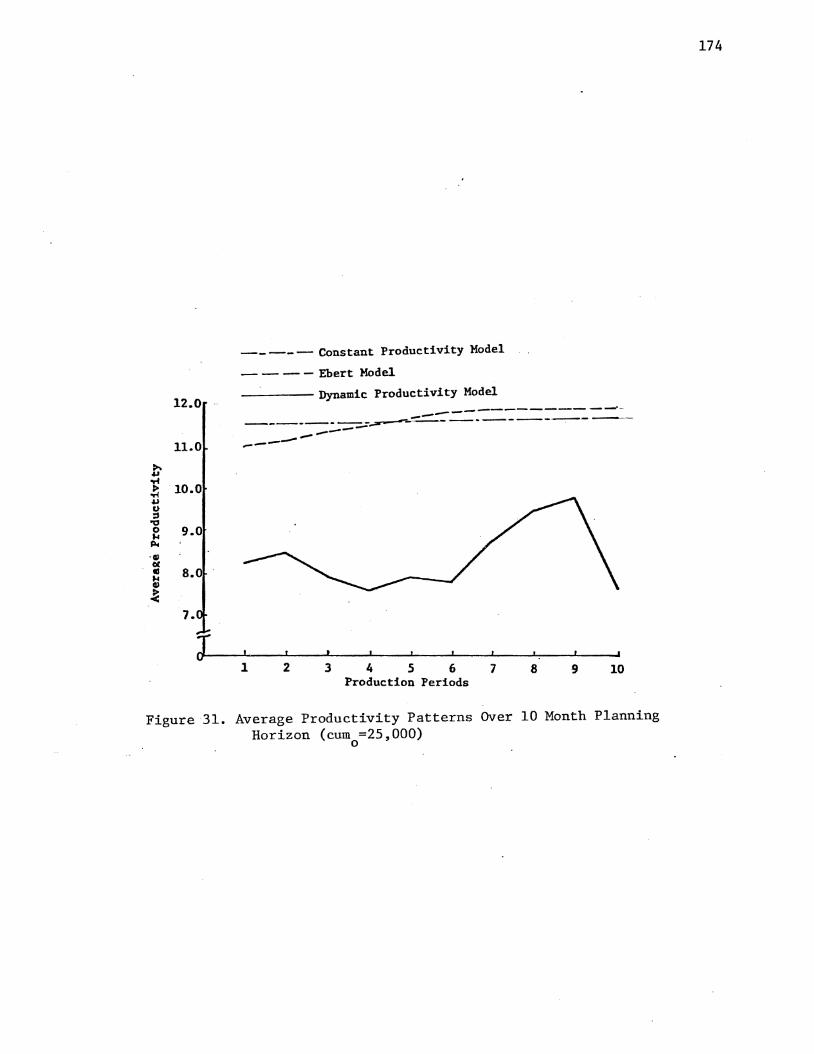
-----Constant Productivity Model

- - -- Ebert Model

12.0 ----------Dynamic Productivity Model

11.0

9.0

8.0

7.

J l 2 3 4 5 6 7 8 9 10

Production Periods

Figure 31. Average Productivity Patterns Over 10 Month Planning Horizon (cum =25,000)

0

174

-----Constant Productivity Model

17.0 -- - - Ebert Model ·

-----Dynamic Productivity Model

16.0 ---------------:;=-~----------~ ------------- -----------

15.0

13.0

12.0

11.0

10.0

9.0

0 T

1 2 3 Production Period

Figure 32. Average Productivity Patterns Over 10 Month Planning Horizon ~(cum =50,000)

0

175

50.0

20.0

10.0

" H 5.0 '-"

cu u c:l ld e 2.0 0

IIH ,.. cu ~ 1.0 cu ~ Ebert Model .., ld 0.5 ..... cu p:

0.2

.05

.02

.01

co 10000 2€1000 30000 ~0000 50000

Product Units

Figur-e 33. Patterns .of--relative Performances oLthe Ebert and_ .the Dynamic Productivity Models Over_ the- Constant·­Productivity Model ·

176

177

the relative performances of the Ebert and the dynamic productivity

models over the constant productivity model as a function of changes in

cum0 • Notice in this figure that the dynamic productivity and the

Ebert models perform slightly better than the constant productivity

model only during the early stages of production. At cum0 =5000 the

relative performance of the dynamic productivity model starts to in­

crease sharply, while the relative performance of the Ebert model con­

tinues to decline.

It should be noted that the cumulative unit number is not the

only factor affecting the relative performance of the new model. Con­

sidering that the impact of this model is d~e to the incorporation of

the significant disruptions resulting from manpower transactions, it

becomes clear that any factor affecting the magnitude of fluctuations

in the workforce level projected by the aggregate plan is an important

factor in this regard. To demonstrate this point, two examples are

given as follow:

One alternative strategy to absorb fluctuations in the demand level

is the utilization of inventories. If the inventory related costs

increase, or storage space becomes a limitation, then less utilization '

of inventories and more utilization of other strategies including the

variations in the manpower level would be justified. A numerical

example shows the impact of this point: Assume that in the paint fac­

tory model the storage space is limited by the maximum capacity of

150 units. This constraint is incorporated into the objective function

of the SDR model. Every time the inventory level exceeds 150, a penalty

of 100,000 is added to the total cost function. The results of optimiza­

tionfor the constant productivity and the dynamic productivity models

178

are given in Table XXI and XXII, respectively. The models are optimized

with respect to an initial cumulative unit number 50,000. Notice the

increased magnitudes of fluctuations in the workforce levels in both

models (compare Table XVII with Table XXI and Table XIX with Table XXII). In

general, the number of the significant disruptions and the magnitude of

each disruption (related to the magnitude of change in the workforce

level) have increased. Also note that, although the number of significant

disruptions is reduced in the dynamic productivity model, the magnitudes

of most disruptions have become larger. The results indicate a better

relative performance of new model over the constant productivity model

(from 26% to 38%).

As in the second example, consider that changes in the cost para­

meter can also affect the fluctuations in the workforce level. For

instance, a decrease in the cost of hiring and firing or an increase

in the overtime cost would result in an increase in the magnitude of

workforce fluctuation. To demonstrate this point numerically, the

parameter c2 (related to the hiring and firing cost) is reduced by one

half and the parameters C3 (related to the overtime cost) is increased

from .2 to 5 in the original paint factory cost model. The Ebert model

and the dynamic productivity model are optimized under the new situation,

and the results are presented in Tables XXIII and XXIV. Notice the great

differences in performance: a 89% better overall result is obtained by

using the new model!

In comparison of Table XXIII with Table XXIV one should note that

although the magnitude of manpower changes in the new model is almost

as large as the magnitude of changes projected by the Ebert model (and·

for the first period is even larger), the new model has scheduled the

Mo.

1 2 3 4 5 6 7 8 9

10

Mo.

1 2 3 4 5 6 7 8 9

10

TABLE XXI

RESULTS OF IMPLEMENTATION OF THE CONSTANT PRODUCTIVITY MODEL (LIMITED INVENTORY)

A. DECISIONS AND PROJECTIONS

Work Proj. Act Demand Force Prod. Inventory Avg Avg

Prod. Prod.

430 46.5 360.1 193.1 16.070 5.800 447 31.7 338.0 84.1 16.070 6.806 440 26.0 338.9 -17.0 16.070 7.026 316 24.7 343.0 10.0 16.070 8.506 397 26.5 532.0 145.0 16.070 8.359 375 23.5 340.0 llO.O 16.070 7.785 292 22.8 332.0 150.0 16.070 9.517 458 24.4 456.8 148.8 16.070 8.422 400 23.1 401.2 150.0 16.070 8.899 350 20.8 298.3 98.3 16.070 7.864

B. COST ANALYSIS OF DECISIONS AND PROJECTIONS

Payroll Hiring & Overtime Inventory Firing

15,798.35 76,685.21 7,020.78 1,328.97 10,782.69 13,992.97 ll,382.26 4,590.56

8,839.45 2,100.41 14,926.03 9,369.89 8,392.43 lll.l5 14,164.94 7,928.66 9,013.82 214.78 39,058.89 2,526.79 7,990.76 582.18 15,737.24 3,638.29 7,764.24 28.54 13' 2ll. 43 2,384.28 8,287.70 152.41 29.193.49 2,417.51 7,860.34 101.59 21,684.74 2,384.33 7,084.71 334.63 13,029.09 4,056.09

179

INDEX ICHK

1 1 1 1 1 1 1 1 1 1 1 1 0 1 1 1 1 1 1 1

($)

Total

200,833.30 40,748.46 35,235.77 30,597.17 50,814.27 27,948.47 23,388.49 40,051.ll 32,030.99 24,504.51

506,152.56

Mo.

1 2 3 4 5 6 7 8 9

10

Mo.

1 2 3 4 5 6 7 8 9

10

TABLE XXII

RESULTS OF OPTIMIZATION (AND IMPLEMENTATION) OF THE DYNAMIC PRODUCTIVITY (LIMITED INVENTORY)

A. DECISIONS AND PROJECTIONS

180

Demand Work Prod. Inventory Avg INDEX ICHK Force Prod.

430 59.9 260.1 93.1 7.037 1 1 447 48.9 438.0 84.1 9.389 1 1 440 41.1 338.9 -17.0 8.258 1 1 316 36.2 343.0 10.0 8.154 1 1 397 34.4 532.0 145.0 10.545 0 1 375 32.7 340.0 110.0 11.450 0 1 393 31.3 332.0 150.0 11.918 0 1 458 32.0 458.0 150.0 12.348 0 1 400 30.7 400.0 150.0 12.729 0 1 350 28.0 250.9 50.9 9.660 1 1

B. COST ANALYSIS OF DECISIONS AND PROJECTIONS ($)

Payroll Hiring & Overtime Inventory Total Firing

20,351.19 28,745.31 1,689.42 4,248.15 55,034.06 16,612.82 7,773.54 8,828.40 4,590.56 37,805.31 13,985.76 3,838.76 5,691.96 9,369.89 32,986.37 12,300.25 1,580.22 7,856.67 7,928.66 29,665.79 11,685.34 210.32 23,333.12 2,526.79 37,755.57 11' 101.10 189.86 8,462.55 3,638.29 23' 391.80 10,650.98 112.70 8,537.47 2,384.28 21,685.43 10,877.85 28.63 15' 251.81 2,384.39 28,542.68

.10,438.70 107.27 11,869.81 2,384.29 24,800.06 9,529.97 459.33 5,047.39 5,975.67 21,012.36

312,679.46

Mo.

1 2 3 4 5 6 7 8 9

10

Mo.

1 2 3 4 5 6 7 8 9

10

TABLE XXIII

RESULTS OF IMPLEMENTATION OF THE EBERT MODEL (MODIFIED COST PARAMETERS)

A. DECISIONS AND PROJECTIONS

Work Proj. Act Demand Force Prod. Inventory Avg Avg

Prod. Prod.

430 43.7 685.5 518.5 15.870 6.780 447 26.3 415.2 486.7 15.959 6.352 440 20.9 333.1 379.9 16.019 6.486 316 20.0 321.4 385.3 16.072 8.907 397 21.1 340.9 329.1 16.125 8.215 375 22.0 356.0 310.2 16.180 9.741 292 22.1 359.7 377.9 16.237 10.419 458 21.9 358.4 278.3 16.294 10.924 400 19.0 310.8 189.0 16.347 8.029 350 15.1 245.8 84.8 16.391 6.121

B. COST ANALYSIS OF DECISIONS AND PROJECTIONS

Payroll Hiring& Overtime Inventory Firing

14,844.73 4,5032.74 781,408.92 3,252.05 8,939.30 8,744.24 321,814.00 2,292.88 7,099.46 945.82 206,629.20 295.61 6,806.49 23.98 113,255.31 351.70 7,174.83 37,91 151,776.69 6.90 7,463.13 23.22 113,148.37 8.00 7,518.45 0.86 95,807.01 276.12 7,436.25 1. 89 83,605.19 143.60 6,445.75 274.13 136,278.35 1,414.72 5,123.02 488.86 126,331.39 4,562.86

181

INDEX ICHK

1 1 1 1 1 1 0 1 1 1 0 1 0 1 0 1 1 1 1 1

($)

Total

844,538.45 342,790.42 214,970,-08 120,437.49 158,996.32 120,642.73 103,602.44

91,186.93 144,412.95 136,396.14

2,277,973.94

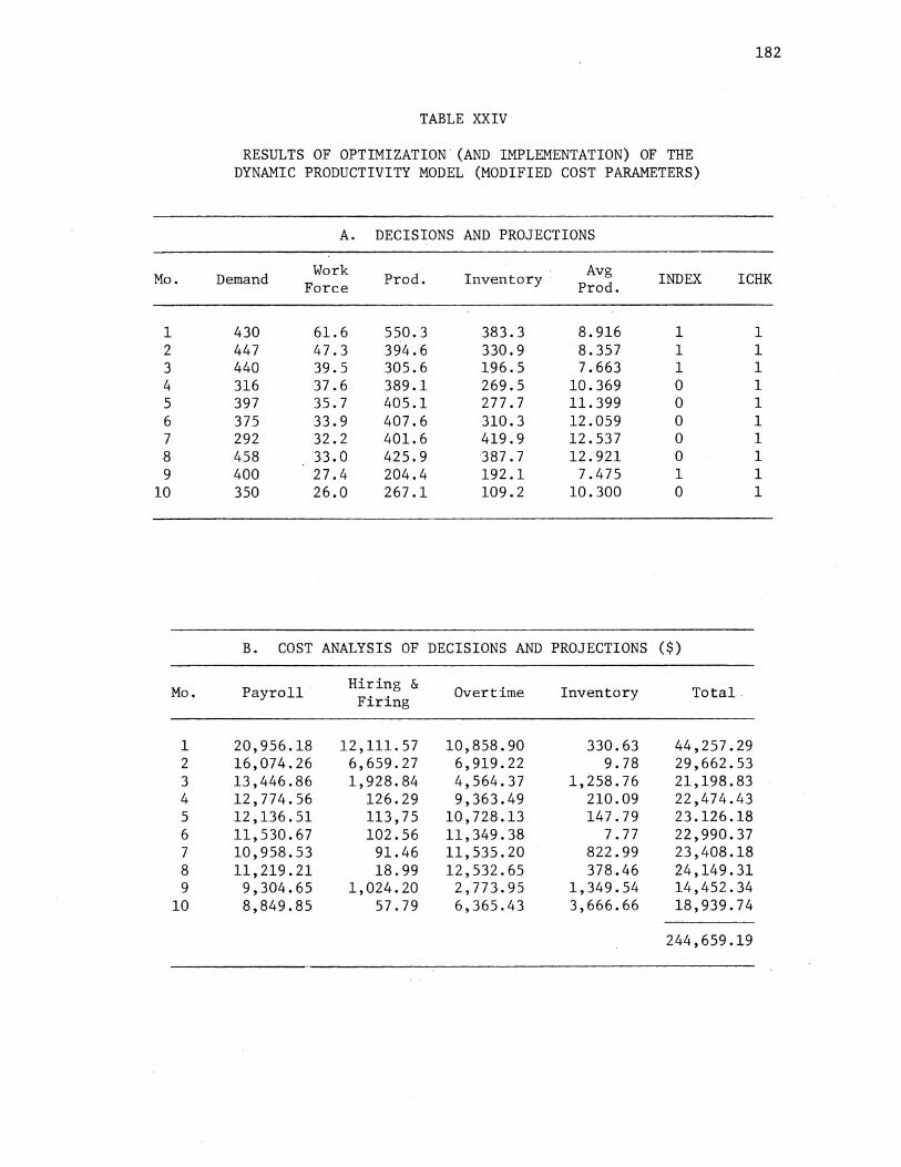
Mo.

1 2 3 4 5 6 7 8 9

10

Mo.

1 2 3 4 5 6 7 8 9

10

TABLE XXIV

RESULTS OF OPTIMIZATION.(AND IMPLEMENTATION) OF THE DYNAMIC PRODUCTIVITY MODEL (MODIFIED COST PARAMETERS)

A. DECISIONS AND PROJECTIONS

182

Demand Work Prod. Inventory Avg INDEX ICHK Force Prod.

430 61.6 550.3 383.3 8.916 1 1 447 47.3 394.6 330.9 8.357 1 1 440 39.5 305.6 196.5 7.663 1 1 316 37.6 389.1 269.5 10.369 0 1 397 35.7 405.1 277.7 11.399 0 1 375 33.9 407.6 310.3 12.059 0 1 292 32.2 401.6 419.9 12.537 0 1 458 33.0 425.9 387.7 12.921 0 1 400 27.4 204.4 192.1 7.475 1 1 350 26.0 267.1 109.2 10.300 0 1

B. COST ANALYSIS OF DECISIONS AND PROJECTIONS ($)

Payroll Hiring & Overtime Inventory Total Firing

20,956.18 12' 111.57 10,858.90 330.63 44,257.29 16,074.26 6,659.27 6,919.22 9.78 29,662.53 13,446.86 1,928.84 4,564.37 1,258.76 21,198.83 12,774.56 126.29 9,363.49 210.09 22,474.43 12,136.51 113' 7 5 10,728.13 147.79 23.126.18 11,530.67 102.56 11,349.38 7. 77 22,990.37 10,958.53 91.46 11,535.20 822.99 23,408.18 11,219.21 18.99 12,532.65 378.46 24,149.31

9,304.65 1,024.20 2,773.95 1,349.54 14,452.34 8,849.85 57.79 6,365.43 3,666.66 18,939.74

244,659.19

183

right timing for these changes. As the result of the arrangement, the

new model incurs lower overtime costs from which the Ebert model has

suffered dramatically.

As the results of the analyses show, the effect of the compounded

disruption is present in most situations. Most disruption effects are

carried over a number of succeeding periods (INDEX and ICHK both take

values of one in most periods). In order to evaluate the significance

of the compounded disruption effects, EPSY is given a high value (100%).

This suppresses the effect of compounded disruption. The problems are

optimized for an initial cumulative unit number of 50,000 for the

original cost structure. Comparing the new results with the ones

presented in Tables XVII to XIX it has been noticed that on the average

a 5% reduction in the total cost has resulted in the constant productiv­

ity, the Ebert, and the dynamic productivity models. This indicates that

the compounded disruption effect, although not considered in the liter­

ature of learning of curve, has significant effect on the production

and workforce planning problems.

Remarks

The foregoing analyses have indicated that the disruption effects

of the manpower transactions on the average productivity significantly

affect the performance of the aggregate planning models. This impact

becomes more severe as the firm approaches its steady production state.

The nature of the cost structure of the firm is also an important factor

reflecting the severity of such effects. The compounded disruption

phenomenon is important and should be considered in production and work­

force planning problems, in general.

184

Anaiysis of Model II

As described in detail in Chapter VI, Model II incorporates new

assumptions and requires new objective function structures. Consequently,

reliable evaluation of the relative performance of this model requires

an existing constant productivity model with similar objective function

structure to serve as a basis for comparison purposes.

Unfortunately, the original HMMS model and other existing aggregate

planning models do not incorporate objective functions with structures

equivalent to the one used in the new model. Aside from the

assumptions regarding the dynamic productivity phenomenon, the new

model differs from most existing models in the way of estimating the

levels for dependent variables such as workforce levels utilized on

regular time, overtime, idle time, subcontracting level, etc. While

the new model computes these level by incorporating proper considera-

tions regarding the production capabilities of the experience classes

involved in different periods, the existing models attempt to approxi-

mate these levels by fitting a polynominal which would hopefully express

the levels for the dependent variables as functions of the independent

decision variables. For example, in the HMMS model, the overtime cost

is approximated by using a quadratic function of the following form:

Overtime cost in period t = c3 (Pt - c4Wt)2 + CsPt - C6Wt

which expresses the cost in terms of production rates and workforce

levels. As Tables IX and X show, this approximation is not always

successful (notice the negative overtime indicated in most periods).

185

For the analysis purposes, the above segment of the cost function

in the HMMS model is changed to a linear function to provide a cost

function somewhat equivalent to the one considered by the new model.

Also, the following simplifying assumptions are made:

Idle workers are assumed to receive the same payments as those assigned on the regular time work. Therefore, this variable is not included in the cost function.

The length of the overtime work is assumed to be 50% of the length of the regular time work.

The hourly overtime payment is assumed to be twice the amount of regular time payment.

Subcontracting is assumed to be allowed.

Based on the above assumptions, the overtime portion of the HMMS

cost model is converted to the following form which also includes the

cost of subcontracting:

overtime and subcontracting costs in period t

where,

WOt = 0 SBt = 0 Wit wt - Pt/C4

(Pt 1

WOt = - C4Wt)f2_C4 SBt 0 = Wit = 0

WOt = Wt 1 SBt (Pt - C4Wt) - 2_C4Wt Wit = 0

if Pt - C4Wt < 0 -

if Pt - C4Wt > 0 and 1

(Pt - C4Wt) - ~4Wt ~ 0

if pt - C4Wt > 0 and 1

(Pt - C4Wt) - ~4Wt > 4

In the above formulation, C1 is the regular payroll cost per employee;

WOt is the workforce level assigned on overtime work in period t; C10 is

the cost of subcontracting per product unit; SBt is the subcontracting

level in period t; C4 is the constant productivity factor (unit output

186

per employee); Wit is the idle workforce level in period t (not

included in the cost function); and Wt and Pt are the workforce level

and the production rate scheduled for period t.

The following relationships explain the above formulation:

C4•Wt - Production capability of the workforce level during regular time work in period t

1 ~4·Wt - Production capability of the workforce level during

overtime work in period t

Pt - C4•Wt - Production level to be allocated to overtime and possibly subcontracting options in period t

Pt/C4 - Workforce level required to produce Pt units

Notice that in this formulation, the productivity rate of employees

during overtime work is assumed to be one half of their productivities

during regular time work. This is because the length of the overtime is

assumed to be one half the length of regular time.

An arbitrary set of data which represent a typical short cycle pro-

duct case is selected. The demand levels assumed in the example problem

are listed in the second column of the following tables. The cost

parameter Cs (related to the inventory cost) in the original HMMS model

is given a new value of 3200 (due to high demand and production quanti-

ties). The cost of subcontracting is assumed to be three dollars per

unit. Slopes of 70%, 90% and 80% are assumed for learning, progress

and forgetting curves, respectively. A base unit cost of .3 man-month

per unit is assumed. The initial inventory level is selected to be

7000 units, and the initial workforce level is 81 men. Initially, a

single experience class with productivity measure of 10 units is

assumed. The overall average productivity for the constant productivity

model is computed over the range of cumulative demand and on the basis

187

of an overall improvement curve with slope of 63% (product of learning

and progress slopes). An initial cumulative unit quantity of 1000

units is assumed. The results of optimization and implementation of the

constant productivity and the dynamic productivity models are presented

in Tables XXV.Aand XXV.B respectively. In this particular example, the

dynamic productivity model performs almost 30% better than the constant

productivity model. Notice the relatively lower workforce levels pro­

jected by the constant productivity model. This is due to the fact that

this model does not incorporate the effect of disruptions in the overall

productivity level. These disruptions are caused by the addition of new

employees with low productivity measures. Also, the forgetting effect

applied to the idle workers is not considered in the constant productiv­

ity model. In general, the constant productivity model assumes relative­

ly higher productivities per employee. Therefore, the workforce level

required to meet the production schedule is relatively lower in this

model.

Further computer runs for different values of the parameters in the

above example have resulted in conclusions similar to most of those

indicated by the analyses of Model I. For example, an increase in the

level of cum0 is accompanied by an increase in the relative performance

of the new model (mainly due to the progress effect). Also, the impact

of the new model becomes more significant for sharper slopes of learning,

progress and forgetting curves.

It should be noted that in this example the total workforce level

in each period is comprised of a number of experience classes each

having different productivity levels. However, the detailed information

regarding the workforce body is not shown in the table.

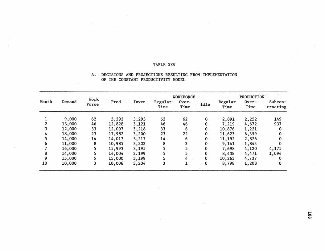
Month Demand

1 9,000 2 13,000 3 12,000 4 18,000 5 14,000 6 11,000 7 16,000 8 14,000 9 15,000

10 10,000

TABLE XXV

A. DECISIONS AND PROJECTIONS RESULTING FROM IMPLEMENTATION OF THE CONSTANT PRODUCTIVITY MODEL

Work WORKFORCE

Force Prod Inven Regular Over- Idle Regular Time Time Time

62 5,292 3,293 62 62 0 2,891 46 12,828 3,121 46 46 0 7,219 33 12,097 3,218 33 6 0 10,876 23 17,982 3,200 23 22 0 11,623 14 14,017 3,217 14 6 0 11,192

8 10,985 3,202 8 3 0 9,141 5 15,993 3,195 5 5 0 7,698 5 14,004 3.199 5 5 0 8,438 5 15,000 3,199 5 4 0 10,263 3 10,006 3,204 3 1 0 8,798

PRODUCTION Over-Time

2,252 4,672 1,221 6,359 2,826 1,843 4,120 4,471 4,737 1,208

Sub con-· tracting

149 937

0 0 0 0

4,175 1,094

0 0

...... 00 00

TABLE XXV (Continued)

B. DECISIONS AND PROJECTIONS OF THE DYNAMIC PRODUCTIVITY MODEL

Work WORKFORCE PRODUCTION Month Demand Force Prod Inven Regular Over- Idle Regular Over- Subcon-

: ;·' Time Time Time Time tracting

1 9,000 69 5,195 3,195 69 55 0 3,200 1,995 0 2 13~000 58 12,987 3,181 58 40 0 8,919 4,067 0 3 12~000 46 12,024 3,205 36 0 9 12,024 0 0 4 18,000 36 17,990 3,195 36 0 0 17,990 0 0 5 i4,000 27 14,005 3,200 20 0 6 14,005 0 0 6 11,000 19 11,002 3,202 12 0 7 11,002 0 0 7 16,000 15 15,995 3,198 15 0 0 15,995 0 0 8 14;000 11 14,004 3,201 10 0 0 14,004 0 0 9 1.5;000 9 14,997 3,199 9 0 0 14,997 0 0

10 10;000 7 10,001 3,200 5 0 1 10,001 0 0 'i

190

As a simple example demonstrating the performance of Model II,

consider a six month planning horizon. Assuming that there are initial­

ly two experience classes with sizes of 40 and 30 men and productivity

measures of 100 and 50, respectively, the results of computations per­

formed by the CLASS routine are listed in Table 25. The input to this

routine are initial status of the experience classes; the values of

the parameters for learning, progress, and forgetting curves (in this

example, these values are 70%, 90% and 80%, respectively; the base unit

cost is assumed to be .3 man-month/unit); and the scheduled values for

the workforce levels and the production rates throughout the planning

horizon.

Table XXVI shows the effects of manpower fluctuations, production

rate fluctuations, regular time work, overtime work, and forgetting on

the conditions of the experience classes in each period. For example,

notice that in the second period the first experience class in the

first period is partitioned into two new classes. This is due to the

assignment of overtime work to the upper part of the class. The

second experience class in the fifth period is partitioned into two

classes in the sixth period as a result of regular time assignment in

this period. Notice the effect of forgetting on the productivity

measrues of idle workers in the fifth·period (the fourth and fifth

classes). The productivity measures of these classes are decreased by

18 and 16 units, respectively, by the end of the sixth period. For

the purpose of simplicity, inventories are not assumed in this example.

Remarks

As Table XXVI indicates, the new model can provide information

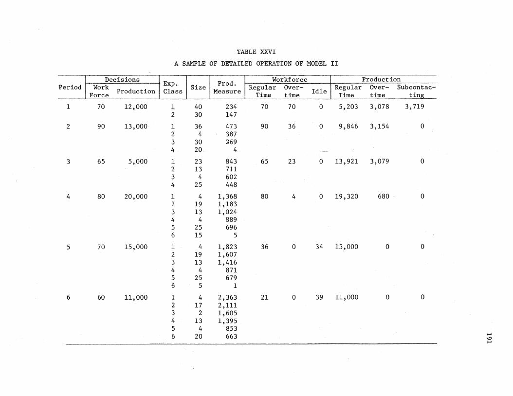
TABLE XXVI

A SAMPLE OF DETAILED OPERATION OF MODEL II

Decisions Exp. Prod. Workforce Production Period Work Size Regular Over- Regular Over- Subcontac-

Force Production Class Measure Time time Idle Time time ting

1 70 12,000 1 40 234 70 70 0 5,203 3,078 3, 719 2 30 147

2 90 13,000 1 36 473 90 36 0 9,846 3,154 0 2 4 387 3 30 269 4 20 4

3 65 5,000 1 23 843 65 23 0 13,921 3,079 0 2 13 711 3 4 602 4 25 448

4 80 20,000 1 4 1,368 80 4 0 19,320 680 0 2 19 1,183 3 13 1,024 4 4 889 5 25 696 6 15 5

5 70 15,000 1 4 1,823 36 0 34 15,000 0 0 2 19 1,607 3 13 1,416 4 4 871 5 25 679 6 5 1

6 60 11,000 1 4 2,363 21 0 39 11,000 0 0 2 17 2,111 3 2 1,605 4 13 1,395 5 4 853 6 20 663 I-'

\0 I-'

192

regarding the size and experience level of each class in each period.

This allows the building of more realistic cost models in which the

regular time, overtime, and idle time payrolls for each class can be

expressed as a function of the productivity level of the class. Also,

as mentioned in Chapter VI, the length of overtime does not have to be

assumed as a constant in the new model. This length (expressed by

OPCNT as a percentage of the regular time length) can be introduced on

an independent decision variable in the new model. The optimum

periodical levels of this variable can then be determined by the

search routine. This would increase the dimension of the problem from

two times the number of periods to three time the number of periods in

the planning horizon.

It should be noted that the special methodologies used for increasing

the computational efficiency of the optimization processes for both

models I and II have been very successful. For example, the stagewise

improvement of the initial solutions in model I optimization has re­

sulted in a computational time saving over 30% for the early stages of

production, where the solution to the Ebert Model is relatively closer

to the dynamic productivity model.

CHAPTER VIII

CONCLUSION AND RECOMMENDATIONS

The aggregate production planning problem is one of the most

challenging and potentially rewarding problems in industry today. The

two-fold economic significance of the problem is by no means minor.

At the micro level, the significance to an individual firm can often

be measured directly in annual savings by following one policy as

opposed to another. On a macro basis, although not often considered

explicitly, the variables considered in aggregate planning form major

factors in the classic economic indicators. The present research

should provide a significant contribution to this area.

The proper incorporation of the dynamic productivity phenomenon

present in most empirical situations into the aggregate production

planning problem has been the main objective of the research. The

research has originated the introduction of workforce level change

disruptions, progress and retrogression effects to this production

planning area. Aggregate planning of both long cycle and short cycle

product cases have been considered and models peculiarto each case have

been developed and analyzed. The analyses of these models indicated

their significant economic impact in the majority of situations. The

relative performances of the new models over the existing ones reach

their highest levels when the productive firm passes the transitional

start-up production period and reaches the steady production state.

193

194

The impact of the models is also subject to the nature of various

operational restrictions imposed on the planning problem, and the

levels of different cost parameters incorporated into the objective

function. The new models hav~ higher impacts for sharper slopes of the

applicable cost reduction curves.

The general solution methodology applied in this research is the

Search Decision Rule. The computer subprograms PROCTV and CLASS

developed for long and short cycle product cases, respectively, are not

peculiar to any specific search technique. Also, the routine developed

for the long cycle product case can be utilized for all existing

aggregate planning cost models. Utilization of the routine developed

for the short cycle product case for the existing cost functions may

require minor modifications in the structure of these functions.

Generally, these programs can serve as standard routines to convert

any current constant productivity aggregate planning model, which applies

the search decision rule, to incorporate the effect of the dynamic

productivity phenomenon. Attachment of the new routines to the existing

programs would require minor modifications in the main and the objective

function routines of these programs to facilitate the process of

transferring the common variables andparameters among the interfacing

routines.

The methodology used for improving the computational efficiency

of the optimizations performed in this research can be generalized for

heuristic optimization of all complex objective functions (provided that

approximation of these functionswithsimpler functions is possible).

The essence of this methodology has been the stagewise approximation of

the cost function and improvement of the starting solutions.

195

Deve£opment of the analysis of the compounded disruption effect is

a significant contribution of this research to the general area of the

improvement curve analysis. Application of the analysis of the com­

poundeddisruption effect is not limited to the aggregate planning

problem. Thiq analysis is useful in a variety of production and work­

force planning and scheduling problems.

Finally, the methodology developed for quantifying the relative

performances of the new models in this research can be used as evalua­

tion methods for future dynamic productivity models.

The following items are recommended for future research:

1. Extension of Models I and II to multi-department aggregate

planning models, in which disruptions as the result of the task changes

generated by the inter-departmental transferring of employees affect

the productivity rates.

2. Substitution of other existing analytical cost reduction curves

in place of the original linear curve models used in this research to

provide models suitable for different industrial applications. For

example, utilization of the mixed model learning curve [66] will be ideal

for the mixed model assembly situations in which more than one model is

assembled on the same assembly line; hence, the repetitions of the as­

sembly work are not always the same. Analysis of various disruption

effects for these cost reduction curves will be required prior to their

incorporation into the dynamic aggregate planning models.

3. Extension of the analysis of Model II for the cost function in

which the payroll costs are expressed as functions of productivity rates

of employees. Also, incorporation of the overtime length as variable

in this model and analysis of the effect of such modifications. These

196

modifications would require a very small programmingeffort since the

provisions have been made in the current program.

4. Incorporation of the integer restric~ion on the variables

such as workforce level into the SDR methodology.

S. Incoxporation of the effects of the dynamic productivity

elements considered in this research (cost reduction, task change dis­

ruption, manpower level change disruption, compounded disruption and

other related elements)intothevarious production, inventory and work

force planning and scheduling areas.

BIBLIOGRAPHY

1. Adler, G. L. and R. Nanda, "The Effect of Learning on Optimal Lot Size Determination- Single Product Case," AilE Transactions, Vol. 6, No. 1 (March 1974), pp. 14-20.

2. Anshen, M., Holt, C. C., Modigliani, F., Muth, J. F. and Simon, H. A., "Mathematics for Production Scheduling," Harvard Business Review, Vol. 36 (1958), pp. 51-58.

3. Asher, Harold, Cost - Quality Relationship in the Airframe Industry, Santa Monica, California, The RAND Corporation, 1956.

4. Balloff, N., "Estimating the Parameters of the Startup Model- An Empirical Approach," Journal of Industrial Engineering, Vol. 18, No. 4 (April 1967), pp. 248-253.

5. Ballof, N., "The Learning Curve - Some Controversial Issues, 1'

Journal of Industrial Economics, (July 1966), pp. 275-282~

6. Bellman, R., "Dynamic Programming and Smoothing Problem," Management Science, Vol. 3, No. 1 (1956), pp. 111-13.

7. Bevis, F. W., Finner, C. and Towill, D. R., "Prediction of Operator Performance During Learning of Repetitive Tasks," International Journal of Production Research, Vol. 8, No. 4 (1970), pp. 293-305.

8. Boeing Company, Improvement Curve, Aero-Space Division, 1963.

9. Boeing Company, Labor Standards Overview, Industrial Engineering, 1977.

10. Boeing Company, Performance Index, Methods Engineering - Industrial Engineering, 1977.

11. Blue, L. R., "An Algorithm for the Vector Maximum Problem," Unpublished Ph.D. Dissertation, University of California, Los Angeles, (1969).

12. Bowman, E. H., "Production Scheduling by the Transportation Method of Linear Programming," Operations Research, Vol. 4, No. 1 (1956), pp. 100-103.

13. Bowman, E. H., "Consistency and Optimality in Managerial Decision Making," Management Science, Vol. 9, No.2 (1963), pp. 310-321.

197

14. Buffa, E. S. and W. H. Taubert, Production - Inventory Systems Planning and Control, Richard D. Irwin, Inc., Homewood, Ill. (1972).

15. Buffa, E. S. and J. G. Miller, Production - Inventory Systems Planning and Control, Richard D. Irwin, Inc.,.Homewood, Ill. (1979).

198

16. Buffa, E. S., and W. H. Taubert, "Evaluation of Direct Computer Search Methods for the Aggregate Planning Problems," Industrial Management Review, M.I.T. Press (Fall, 1967), pp. 19-36.

17. Carlson, J. G. and A. J. Rowe, "How Much Does Forgetting Cost?", Industrial Engineering, (September, 1976), pp. 40-47.

18. Chang, H. R. and C. M. Jones, "Production and Work Force Scheduling Extensions," AilE Transactions, Vol. 2, No. 4 (1970), pp. 326-33.

~_0 Cochran, E. B., Planning Production Costs: Using the Improvement Curve, Chalender Publishing Co., 1968.

20.

21.

22.

23.

25.

Cochran, E. B., "New Concepts of the Learning Curve," Journal of Industrial Engineering, (July-August, 1960), pp. 317-327.

Conway, R. W., and Schultz, A. J., "The Manufacturing Progress Function," Journal of Industrial Engineering, (January-February, 1956), pp. 39-54.

Davidson, W. C., "Variable Metric Method of Minimization," AEC Research and Development Report, ANL-5990 (Rev.), (195F.

DeJong, J. R., "The Effects of Increasing Skills on Cycle Time and Its Consequences for Time Standards," Ergonomics, Vol. 1, No. 1, (1957), pp. 51-60.

Ebert, R. J., "Aggregate Planning with Learning Curve Productivity," Management Science, Vol. 23 (1976), pp. 171-182.

Ebert, R. J., "Time Horizon: Implementations for Agregate Scheduling Effectiveness," AilE Transactions, Vol. 4, No. 4 (1972) pp. 298-307.

26. Eilon, S., "Five Approaches to Aggregate Production Planning," AilE Transactions, Vol. 7, No. 2 (1975), pp. 118-131.

27. Fletcher, R., and M. Powell, "A Convergent Descent Method for Minimization," The Computer Journal, Vol. 6 (1963), pp. 163-168.

28. Fletcher, R. and C. Reeves, "Function Minimization by Conjugate Gradients," The Computer Journal, Vol. 7 (1964)., pp. 149-154.

29. Gaalman, G. J., "Optimal Aggregation of Multi-Item Production Smoothing Models," Management Science, Vol. 24 (1979), pp. 1733-39.

\}

v

199

30. Goodman, D. A., "A New Approach to Scheduling Aggregate Production. Work Force," AilE Transactions, (June 1973), pp. 135-141.

31. Goodman, D. A., "A Goal Programming Approach to Aggregate Planning of Production and Work Force," Management Science, Vol. 20, No. 12 (1974), pp. 1569-1575.

32. Gordon', J. R. M., A Multi-Model Analysis of an Aggregate Scheduling Decisions, Unpublished Ph.D. dissertation, Sloan School of Management, MIT, 1966.

33. Greene, J. H., Production and Inventory Control, Richard D. Irwin, Inc., Homewood, Ill., 1974.

v34. Hanssmann, F. , and S. W. Hess, "A Linear Programming Approach to Production and Employment Scheduling," Management Technology, No. 1 (January, 1960), pp. 46-51.

35. Hirshmann, W. V., "Profit From the Learning Curve," Harvard Business Review, Vol. 42 (1964), pp. 125-139.

36. Hoffman, T. R., "Effect of Prior Experience on Learning Curve Parameters," Journal of Industrial Engineering, (August, 1968), pp. 317-327.

37. Holt, C. C., Modigliani, F., Muth, J. F., and Simon, H. A., Planning Production Inventories and Workforce, Prentice-Hall, Englewood Cliffs, N.J., 1960.

38. Hooke, R. and Jeeves, T. A., "Direct Search Solution of Numerical and Statistical Problems," Journal of the Association for Computing Machinery, Vol. 8 (1961), pp. 212-229.

39. Johnson, L.A. and Montgomery, D. C., Operations Research in Production Planning, Scheduling, and Inventory Control, V John Wiley and Sons, Inc., 1974.

40. Jones, C. H., "Parametric Production Planning," Management Science, Vol. 13, No. 11 (1967), pp. 843-66.

41. Kleindorfer, P. and H. Kunreuther, "Stochastic Horizons for the Aggregate Planning Problem," Management Science, Vol. 24, No. 5 (1978), pp. 485-497.

42. Kolesar, P., "A Branch and Bound Algorithm for the Knapsack Problem," Management Science, Vol, 13, No. 9 (1967), pp. 723-735.

43. Korgaonker, M. G., "Production Smoothing Under Piecewise Concave Costs, Capacity Constraints and Nondecreasing Requirements," Management Science, Vol. 24, No. 3 (1977), pp. 302-311.

44. Kuester, J. L. and Mize, J. H., Optimization Techniques with Fortran, McGraw-Hill Book Co., 1973.

45. Kunreuther, H. C. and Morton, T. W., "Planning Horizon for Prod­uction Smoothing with Deterministic Demands," Management Science, Vol. 20, No. 1 (1973), pp. 110-125.

46. Levy, F. K., "Adaptation in the Production Process," Management Sciences, Vol. 11, No. 6 (1965), pp. B-136-151.

47. McGarrah, R. E., Production and Logistics Management: Text and Cases, New York: John Wiley and Sons, INc., 1963 .

200

48. Mize, J. H., C. R. White and G. H. Brooks, Operations Pl\;;lnning and Control, Prentice-Hall, Inc., Englewood Cliffs, N.J., (1971).

49. Moskowitz, H., "The Value of Ttiformation in Aggregate Planning - A Behavioral Experiment," AilE Transactions, Vol. 4, No. 4 (1972), pp. 290-297.

50. Nada, R. and A. Georgel, Learning Curves Theory and Application, WM & ME Monograph Series No. 6, AIIE-WM & ME, 1977.

51. Nelder, J. A., and R. Meads, "A Simplex Method for Function Minimization," Computer Journal, Vol. 7 (1964), pp. 308-315.

52. Niland, P., Production Planning, Scheduling, and Inventory Control, MacMillan, London, 1970.

V.S3. Orrbeck, M. G., Schwette, D. R., and Thompson, H. E., "The Effect of Worker Productivity on Production Smoothing," Management Science, Vol. 14 (1968), pp. 332-342.

54. Pegels, C. C., "Work Force Planning for the Job Shop," The Logistic Review, Vol. 5, No. 21 (1969), pp. 41-49.

55. Pegels, C. C., "On Startup or Learning Curves: An Expanded View," AilE Transactions, Vol. 1, No. 3 (1969), pp. 216-222.

56. Pegels, C. C., System Analysis for Production Operations, Gordon and Breach Publishers, Inc., New York, N.Y., 1976.

57. t/ Petersen, E. R., "A Dynamic P.rogramming· Model for the Expansion of Electric Power Systems," Management Science, Vol. 20, No.4 (December, Part II, 1973), pp. 656-673.

58. Plossl, G. W. and Wight, 0. W., Production and Inventory Control Principles and Techniques, Prentice-Hall, Inc., Englewood Cliffs, N.J., 1967.

59. Schwarz, L. B. and Johnson, R. E., "An Appraisal of the Emperical· Performance of the Linear Decision Rule for Aggregate Planning," Management Science, Vol. 24 (1978), pp. 844-849.

60. Sikes, T. W., "The Search Decision Rule Applied to Aggregate Planning: Improved Efficiency and Stochastic Extension," Unpublished Ph.D. Dissertation, UCLA.(August, 1970).

61. Silver, E. A. "A Tutorical on Production Smoothing and Workforce Balancing," Operations Research, (November-December, 1967), pp. 985-1011.

201

62. Stanford Research Institute SRI (3), Relationships for Determining the Optimum Expansibility of the Elements of a Peacetime Air­craft Procurement Program, (for USAF-AMC), December, 1949.

63. Sypkens, H. A., Planning for Optimal Plant Capacity, Master's Thesis Sloan School of Management, MIT, 1967.

64. Taubert, W. H., "A Search Decision Rule for the Aggregate Scheduling Problem," Management Science, Vol. 14, No.6 (1968), pp. 343-59.

v 65. Taubert, W. H., "The Search Decision Rule Approach to Operations Planning," Unpublished Ph.D. Dissertation, UCLA, (1968).

66. Thomopoulos, N. T. and M. Lehman, "The Mixed Model Learning Curve," AIIE Transactions, Vol. 1, No. 2 (1969), pp. 127-132.

67. Van de Panne, C. and Bose, P., "Sensitivity Analysis of Cost Coefficient Estimates: The Case of Linear Decisions Rules for Employment and Production," Management Science, Vol. 9, (1962) pp. 82-107.

68. Vergin, R. C., "Production Scheduling Under Seasonal Demand," Journal of Industrial Engineering, (May 1966), pp. 260-266.

69. Weismann, J., Wood, C. F., and Rivlin, L., "Optimal Design of Chemical Process Systems," Chemical Engineering Progress Symposium Series, Process Control and Applied Mathematics, Vol. 61, No. 55 (1965), pp. 50-63.

70. Wolfe, P.M., B. Khoshnevis, M. P. Terrell and R. Monjazeb, "Aggregate Planning Models Incorporating Productivity - V An Overview," Transactions of the American Institute of Industrial Engineers Conference, (May, 1979), pp. 280-283.

71. Wright, T. P., "Factors Affecting the Cost of Airplanes," Journal of the Aeronautical Sciences, Vol. 3 (February, 1936), pp. 275-282.

72. Zangwill, W. J., Minimizing a Function Without Calculating Deviations," The Computer Journal, (1967), pp. 293-296.

APPENDIX A

GLOSSARY OF VARIABLES USED IN COMPUTER PROGRAM

FOR MODEL-I (EXCLUDING THE SEARCH ROUTINE)

202

APROD(I)

AKl, AK2

AK3

B

BCT(I)

CAPR

CUM(I)

CUM~

Cl

C2

C3, C5 & C6

C7 & CB

C9 & ClO

D(I)

DINV(I)

DPCST(I)

EPSY

F

HLCST(I)

I

Average productivity in the ith period computed by PROCT routine

203

Constants used to delute the task turnover in cases of manpower reduction and addition

Constant used to delute the task turnover in case of manpower reduction

Measure (exponent) of slope for improvement curve

Block cost in the ith period

Overall average productivity applied by the con­stant productivity model

Cumulative number of units produced by the end of the ith period

Cumulative number of units produced by the begin­ning of the first period

Cost coefficient for direct payroll cost

Cost coefficient for hiring and firing costs

Cost coefficients for overtime cost

Cost coefficients for inventory carrying cost

Additional cost coefficients (not used in this model)

Demand level in the ith period

Inventory level in the ith period

Direct payroll cost in the ith period

a minimum unit cost difference level above which the current disruption is assumed to be carried over to ·the following period

Base unit cost (in terms of man-month)

Hiring and layoff cost in the ith period

A localized index for various loops; generally represents the period number for the consecutive periods.

ICHK(I)

ICNTRL

IEFECT

INDEX(I)

IP

KFLAG

KPRESS

KPRINT

LIM

N

NEVAL

NM

204

A binary variable used to record the occurance of compound disruption; it is 0 if the unit cost difference at the end of the ith period is less than EPSY; it is 1, otherwise

A flag used in detecting IEFECT. It is 1 as long as a change in the level of independent variables is not reported; it becomes 2 as soon as a change is detected

The period number at which the first change in the level of an independent variable is made by the search routine. It is used for gaining computational efficiency

A binary variable used to record the occurances of significant disruptions. It is 1 if the disruption occuring at the beginning of the ith period is significant; it is 0, otherwise

An index used to update the level of the cumulative number of units when a change is made in the level of production rate in a period

A flag used to direct the control in PROCTIV and FCTl. If KGLAG = 0, the dynamic productivity model is in effect. If KFLAG = 1, the constant productivity model in in effect. If KFLAG = 2, the Ebert model is in effect.

A variable which when set =1, suppresses a large portion of the detailed output of the search routine (see Appendix C)

A flag controlling the printout in the main routine. It directs the control for printing the results of optimization and evaluation of the three models considered.

An approximate upper bound on the number of calls of the objective functions (see Appendix C)

The number of independent variables in the search, N = 2*NM

Number of function evaluations (see Appendix C)

Computer system input unit code

Number of periods in the planning horizon--length of the planning horizon

NO

OINV

OVCST(I)

P(I)

PCUM

R(I)

s

SN

STCST(I)

TC(I)

TDND

TMHR

TNMP(I)

TOT CST

TRSHL

UA

UB

UCDIF(I)

UC(K)

Computer system output unit code

Initial level of inventory (at the beginning of the first period)

Overtime cost in the ith period

205

Production rate in the ith period (an independent variable)

A localized variable used in computing the cumula­tive number of units

Task turnover ratio considered for the beginning of the ith period

Slope of the improvement curve

The response level of the objective function

Storage (inventory) cost in the ith period

Total operation costs in the ith period

A localized variable used in computing total demand for the constant productivity model

Total man-month requirement (block cost) over the planning horizon. It is used in computing the average productivity level for the constant productivity model

Manpower turnover in the ith period (undeluted)

Total cost of operations throughout the planning horizon

The threshold level for significant disruption

The cumulative unit number received by UNIT and BLOCK. If received by BLOCK, UA is the first unit number in the block of units

The cumulative unit number received by BLOCK. It is the last unit number in the block of units

The unit cost difference at the end of the ith period

A localized value used to compute the unit cost of the Kth unit in sequence of units

UCT(I)

ux

UY

uz

W(I)

WOLD

X(J)

XMAX(J)

XMIN(j)

ZADJ

Unit cost of the last unit produced in the ith period

206

1\ localized variable representing the cumulative unit number at which a 'carried over' disruption takes place

A localized variable representing the cumulative unit number of the first unit produced in a period

A localized variable representing the cumulative unit number of the last unit produced in a period

Workforce level in the ith period (an independent variable

A localized variable representing the workforce l~vel in the previous period (=W(I-1))

Initial workforce level

The jth independent variable (see Appendix C)

Upper limit on jth independent variable, X(j)

Lower limit on jth independent variable, X(j)

The unit cost difference ratio at the end of the first period, used to adjust the task turnover for the beginning of the first period in the next month optimization

APPENDIX B

GLOSSARY OF VARIABLES USED IN COMPUTER PROGRAM

FOR MODEL-II (EXCLUDING THE SEARCH ROUTINE)

207

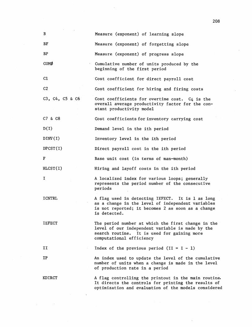
B

BF

BP

COM0

Cl

C2

C3, C4, CS & C6

C7 & C8

D(I)

DINV(I)

DPCST(I)

F

HLCST(I)

I

ICNTRL

IEFECT

II

IP

KDIRCT

Measure (exponent) of learning slope

Measure (exponent) of forgetting slope

Measure (exponent) of progress slope

Cumulative number of units produced by the beginning of the first period

Cost coefficient for direct payroll cost

Cost coefficient for hiring and firing costs

Cost coefficients for overtime cost. C4 is the overall average productivity factor for the con­stant productivity model

Cost coefficients for inventory carrying cost

Demand level in the ith period

Inventory level in the ith period

Direct payroll cost in the ith period

Base unit cost (in terms of man-month)

Hiring and layoff costs in the ith period

A localized index for various loops; generally represents the period number of the consecutive periods

208

A flag used in detecting IEFECT. It is 1 as long as a change in the level of independent variables is not reported; it becomes 2 as soon as a change is detected.

The period number at which the first change in the level of our independent variable is made by the search routine. It is used for gaining more computational efficiency

Index of the previous period (II = I - 1)

An index used to update the level of the cumulative number of units when a change is made in the level of production rate in a period

A flag controlling the printout in the main routine. It directs the controls for printing the results of optimization and evaluation of the models considered

KFLAG

KPRESS

LIM

N

NEVAL

NI

NM

NO

NTEMP

NXCL(I)

NXCL0

NXX

OINV

OPCNT

OVCST(I)

P(I)

PCUM

PCXR(I,J)

209

A flag used to direct the control in CLASS. If KFLAG = 0, class partition does not apply; other­wise, KFLAG = 1.

A variable which when set =1, suppresses a large portion of the detailed output of the search routine (see Appendix C)

An approximate upper bound on the number of calls of the objective function (see Appendix C)

The number of independent variables in the search, N = 2*NM

Number of function evaluations (see Appendix C)

Computer system input unit code

Number of periods in the planning horizon--the length of the planning horizon

Computer system output unit code

A temporary location for the number of experience classes. NTEMP is updated if a class partition takes place

Number of experience classes in the ith period. NXCL takes the updated value of NTEMP

Initial number of experience classes (at the beginning of the first period)

A localized variable used to compute NTEMP

Initial inventory level

The length of overtime as percentage of the length of regular time

Overtime cost in the ith period

Production rate in the ith period (an independent variable)

A localized variable used in computing the cumulative number of units

Production capability of the jth experience class in the ith period

PNALT(I)

POVR(I)

PREG(I)

RP

SF

SL

SN

SP

ss

STCST(I)

SUB(I)

TDND

TL

TMHR

TOT CST

TWO

210

A binary variable recording the violation of the total production capability constraint. When this constraint is violated in the ith period, PNALT(I) is set equal to 1, otherwise it is zero. This variable is multiplied by ClO and the result is incorporated into the objective function

Total production on overtime in the ith period

Total production on regular time in the ith period

A localized variable representing the remaining (excess) production level. It is used in com­puting PREG, POVER, size of partitioned classes, and the subcontracting level

Slope of forgetting

Slope of learning

The response level of the objective function

Slope of progress

Slope of the overall improvement curve (used in the constant productivity model)

Storage (inventory) cost in the ith period

Subcontracting level in the ith period

A localized variable used to compute the total demand for the constant productivity model

A localized variable accumuiating numbers of men in the sequentially taken experience ·classes. It is used to incorporate the effect of manpower reduction

Total man-month required (block cost) over the planning horizon. It is used in computing the average productivity level for the constant productivity model

Total operating cost throughout the planning horizon

A localized variable representing the total number of men assigned on overtime work (in a period)

TWR

UF

UP

UPP

UTEMP(J)

UXCL(I,J)

UXCL~(J)

UXX(J)

W(I)

WIDL(I)

WL

WOLD

WOVR(I)

WREG(I)

WRDP

WRRP

WTEMP(J)

WXCL(I,J)

211

A localized variable representing the total number of men assigned on regular time work (in a period)

Level of the productivity measure at which for­getting starts

The applicable cumulative unit number for which the progress effect ( UPP) is computed.

Progress effect factor

A temporary location for productivity measure of the jth class (in a period)

Productivity measure of the jth experience class in the ith period

Initial level of productivity measure of the jth experience class

A localized variable used for storing the produc~ tivity measure of the j th experience class ·

Workforce level in the ith period (an independent variable)

Total number of idle men in the ith period

A localized variable representing the amount of change in the total level of manpower

A localized variable representing the workforce level in the previous period

Total number of men assigned on overtime work in the ith period

Total number of men assigned on regular time work in the ith period

The size of upper portion of the class partitioned through assignment of overtime

The size of upper portion of the class partitioned through assignment of regular time

A temporary location for storing the number of members in the jth experience class

The size of the jth experience class in the ith period

WXCL0(J)

WXX(j)

X(K)

XMAX(K)

XMIN(K)

212

Initial size of the jth experience class

A localized variable used for storing the size of the jth experience class (in a period)

The kth independent variable (see Appendix C)

Upper limit on kth independent variable, X(K)

Lower limit on kth independent variable, X(K)

APPENDIX C

GLOSSARY OF VARIABLES USED IN

PATTERN SEARCH SUBROUTINE

213

ALP

BET

D(I)

DEL

DX

Dl

GR

I

IDl

ID2

ID3

ID4

ITR

K

Alpha, the factor by which the step size, D(I), grows when a forward move is successful and L4 = 2. (Initialized at 2.0; used in stm 292)

214

Beta, the multiplicative factor by which step size for an independent variable is reduced if forward and reverse move for that variable fail

The current value of the step size for the ith independent variable

Delta, the multiplier which is used to determine the initial value of D(I), the step size, in accordance with statement 180

A local quantity used to determine whether the lower bound on the step size has been reached. DX is computed and used only between stms 480 and 485, where step size reduction takes place

A quantity used to increment the value of GR in the adaptive logic. Dl is set in stms 802 + 1 and 804; it is used in stm 810

The factor by which the pattern move vector is multiplied to obtain the actual size of the pat­tern move. (GR is initialized at 2.2 and adjusted upward, usually by increment of .1, in statements 510 through 783.) When GR reaches 3.5 it is reset to 2.2

A highly localized variable used as an index in DO loops--see stms 180, 420, 786

Counter to record passes through stm 802

Counter to record passes through stm 803

Counter to record passes through stm 804

Counter to record passes through stm 801

A· printout control character of little importance; initialized at 1 and left at that value. It is tested in stm 888; if the value is >1 it causes deletion of certain print lines. (In effect, it is not used unless initialized at ITR > 1.)

A subscript which defines which independent variable is now being studied--as in X(K), D(K), etc.

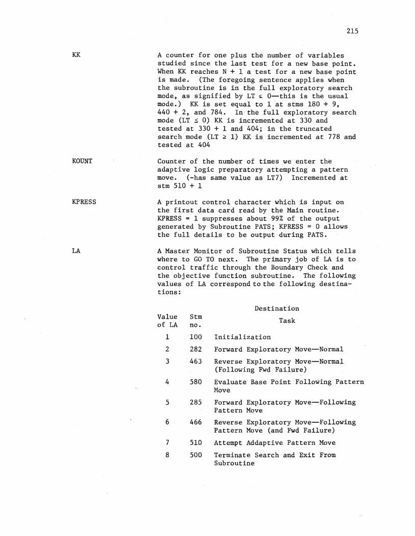
KK

KOUNT

KPRESS

LA

215

A counter for one plus the number of variables studied since the last test for a new base point. When KK reaches N + 1 a test for a new base point is made. (The foregoing sentence applies when the subroutine is in the full exploratory search mode, as signified by LT ~ 0--this is the usual mode.) KK is set equal to 1 at stms 180 + 9, 440 + 2, and 784. In the full exploratory search mode (LT ~ 0) KK is incremented at 330 and tested at 330 + 1 and 404; in the truncated search mode (LT ~ 1) KK is incremented at 778 and tested at 404

Counter of the number of times we enter the adaptive logic preparatory attempting a pattern move. (-has same value as LT7) Incremented at stm 510 + 1

A printout control character which is input on the first data card read by the Main routine. KPRESS = 1 suppresses about 99% of the output generated by Subroutine PATS; KPRESS = 0 allows the full details to be output during PATS.

A Master Monitor of Subroutine Status which tells where to GO TO next. The primary job of LA is to control traffic through the Boundary Check and the objective function subroutine. The following values of LA correspond to the following destina­tions:

Value Stm of LA no.

1 100

2 282

3 . 463

4 580

5

6

7

8

285

466

510

500

Destination

Task

Initialization

Forward Exploratory Move--Normal

Reverse Exploratory Move--Normal. (Following Fwd Failure)

Evaluate Base Point Following Pattern Move

Forward Exploratory Move--Following Pattern Move

Reverse Exploratory Move--Following Pattern Move (and Fwd Failure)

Attempt Addaptive Pattern Move

Terminate Search and Exit From Subroutine

LIM

LSN

LT

LT2

LT3

LT4

LT5

LT6

LT7

216

An approximate upper bound on the number of calls of the objective function during a particular call of subroutine PATS. (LIM is usually set at 3000, but a different value might be appropriate for some applications.) See final remark under NEVAL for identification of location where NEVAL is tested

Set at 0 in fifth statement of subroutine and kept there--never referred to again except in statement 784 + 1 (See Weisman, Wood, and Rivlin for explanation)

Controls the choice between the standard full exploratory search mode (LT ~ 0) and the truncated search mode (LT ~ 1). Under truncated mode the exploratory search is stopped as soon as any move produces an improvement in the last base point. This point is saved as the new base point, and a pattern move is made. The next exploratory search starts with the variable after the one which produced the last success. Under the full exploratory search mode, which is the mode this coding reflects, since LT = 0, an exploratory step is made with all N variables before a pattern move is attempted. LT is set in the fourth statement of the subroutine and does not appear again except in statement 320 and 400.

Number of times this subroutine has reached status LA= 2*

Number of times this subroutine has reached status LA= 3*

Number of times this subroutine has reached status LA = 4

Number of times this subroutine has reached status LA = 5*

Number of times this subroutine has reached status LA = 6*

Number of times this subroutine has reached status LA = 7

*in the event that a proposed forward or reverse move fails the boundary check the appropriate one of the coutners will fail to be incremented

14

Ml

M2

N

NEVAL

NEVOLD

A status variable always equal to 1 or 2: 14 - 1 says we are in the process of making exploratory moves in normal fashion, i.e., we are searching for a pattern. 14 = 2 says we are in the process of making exploratory moves following a pattern move

217

One plus the number of indpendent variables which have experienced both forward and reverse failures with the minimum step size since the last test for a new base point. The search is terminated when Ml is ~ N + 1 during the exploratory search mode, i.e., when 14 = 1 and we are attempting to establish a new pattern. Even though Ml may be (redundantly) manipulated while the search is conducting a post-pattern-move exploration (when 14 = 2), it is never used, i.e., tested, ~cept when we are attempting to establish a new pattern, namely when L4·= 1. (In reprogramming, this variable could be reduced by 1, i.e., intialized to 0 and tested for ~ n, with improved clarity of interpretation; this also applies to M2.) Ml is initialized in stms 180 + 6, 300 + 2, 352 + 1, and 440 + 1; incremented at 490; and tested at 429 + 1

One plus the number of independent variables which have experienced both forward and reverse failures since the last attempt to make a pattern move. The pattern is considered broken and the search is restored to exploratory mode (L4's value changes from 2 to 1) if all variables fail following a single pattern move attempt

The number of independent variables, i.e., the dimensionality of the space being searched.

A counter of the number of evulatuation of FCTl, the objective function, which have been made during this particular call of Subroutine PATS. NEVAL is incremented inside Subroutine FCTl; it is not tested every time it is incremented. LIM is an approximate upper bound on NEVAL; the test is made in stm 7, just prior to attempting a pattern move. This is preferable to testing every time FCTl is called

Variable used to store the previous value of NEVAL, the "total number of evaluation of the objective function made thus far." NEVOLD is reset at stm 815 + 2 and is used in the computa­tion of V in stm 398

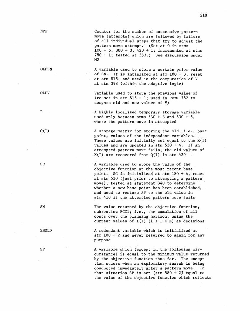
NPF

OLDSN

OLDV

p

Q(I)

sc

SN

SNOLD

SP

218

Counter for the number of successive pattern move (attempts) which are followed by failure of all individual steps that try to adjust the pattern move attempt. (Set at 0 in stms 100 + 5, 300 + 3, 420 + 1; incremented at stms 780 + 1; tested at 353.) See discussion under M2

A variable used to store a certain prior value of SN. It is intialized at stm 180 + 3, reset at stm 815, and used in the computation of V at stm 398 (within the adaptive logic)

Variable used to store the previous value of (re-set in stm 815 + 1; used in stm 782 to compare old and new values of V)

A highly localized temporary storage variable used only between stms 530 + 3 and 530 + 5, where the pattern move is attempted

A storage matrix for storing the old, i.e., base point, values of the independent variables. These values are initially set equal to the X(I) values and are updated in stm 530 + 4. If an attempted pattern move fails, the old values of X(I) are recovered from Q(I) in stm 420

A variable used to store the value of the objective function at the most recent base point. SC is initializeq at stm 180 + 4, reset at stm 530 (just prior to attempting a pattern move), tested at statement 340 to determine whether a new base point has been established, and used to restore SP to the old value in stm 410 if the attempted pattern move fails

The value returned by the objective function, subroutine FCTl; i.e., the cumulation of all costs over the planning horizon, using the current values of X(I) (1 $ I ~ N) as decisions

A redundant variable which is initialized at stm 180 + 2 and never referred to again for any purpose

A variable which (except in the following cir­cumstance) is equal to the minimum value returned by the objective function thus far. The excep­tion occurs when an exploratory search is being conducted immediately after a pattern move. In that situation SP is set (stm 580 + 2} equal to the value of the objective function which reflects

TOL

v

X(I)

XMAX(I)

XMIN(I)

219

the unadjusted pattern move, and thereafter, as the exploratory search to adjust the pattern move proceeds, SP is updated to reflect the m1n1mum of this value and the best exploratory move to date. After the explorations are com­pleted, this updated value of SP is compared (stm 340) with SC, the value of the objective function at the last base point. If this base point test is passed, the (adjusted) pattern move is declared successful and a new base point is established. If the base point test is not passed, the pattern move attempt is declared unsuccessful, SP is restored to its old value (stm 410), and local explorations are initiated about the old base point in an effort to esta­blish a new pattern

A quantity used (stm 480 + 2) in obtaining lower bounds on step sized for exploratory moves

Percentage improvement in value of objective function per call of objective function. Com­puted and used in adaptive logic--see stms 398 through 782

The independent decision variables (of which ther are N: 1 ~I~ N). In the Paint Factory application the odd values of the index, I, identify the work force decisions in successive months, while the even values of the index denote production rate decisions for those months. There are N/2 months in the planning horizon

The upper bound on the acceptable value of X(I)

The lower bound on the acceptable value of X(I)

APPENDIX D

SEMI-DESCRIPTIVE FLOWCHARTS OF

COMPUTER PROGRAM FOR MODEL-I

220

221

( MAIN ) l

READ P AIWf!'l'I!RS POR Til! SEARCH ROUTINE')

! READ IRJMI!R OF PERIODS J AND DI!IWID PER PERIOO

1 READ STARTING VALUES, LOWER AND I

UPPER BOUNDS POR DI!CISION VARIABLES

1 READ PAIWIETI!RS OF '111! COST FUNCTION '1

1 READ PAIWIETI!RS OF IMPROVEMENT CURVJ!: 1

BASE UNIT AND SLOPE

! READ PAIWI!TERS FOR MANPOW!R I

TRANSACTIONS AND C<I!POUND DISRUPTION Kl, JC2, 10, TRSHL, !PST

1 READ INITIAL CUM. UNIT NO.,

INITIAL WORKFORCE L!VBL INTITIAL INVENTORY AND DESIRED

ENDING INVENTORY LBVI!LS

! COIPUTE B FACTOR POl Til! IMPROVDIBIIT CURVB

• ·l

COMPlJ'fB OVI!RALL AVERAGE PRODUCTIVITY ON THE BASIS OF TOTAL DI!HAND AND TIIB CURllBNT DIPROVI!MENT CURV! PARAKETI!RS

PURPOSE: TO B! USED FOR EVALUATION OP CONSTANT

PRODUCTIVITY MODBLS

cb

222

[ ~

KFLAG•l: NO RErEilENCE TO PROCTIV

l I CALL PATS: OPT~IZE CONSTANT I PRODUCTIVITY mDEL

l ll'RINT-1 r--

l lti'UG-0: PROCTIV IN J!llnCT• ICPRINT-2

l INITIALIZE W I) 6 P (I : CLEAR I!PI!CT

_1

I . CALL FCTl ~ EVALUATE THE CONSTAIIT PROD. MODEL

t ULAC-2· NO DISRUPTIOR· KPRINT-3 I

liNITIALIZE W(I) & P n' CLEAR IBFI!CT

NEVAL-0

~

I CALL PATS; OPTIMIZE ~ EBERT MODEL

l r----i_UI.AG-0· PROCTIV IN EFPBCT• JCPRINT-4

INITIALIZE W I 6 p I • CLEAR IBFI!CT

2

I CALL FCTl J--EVALUATE EBERT MODIL

t -+1. ICPRINT-5-• INITIALIZE W I ' p I

l 3 NEVAL-0

l CALL PATS· OPTIMIZE MODEL I

PRINT RESULTS

4 ~ ICPRINT9 >

G

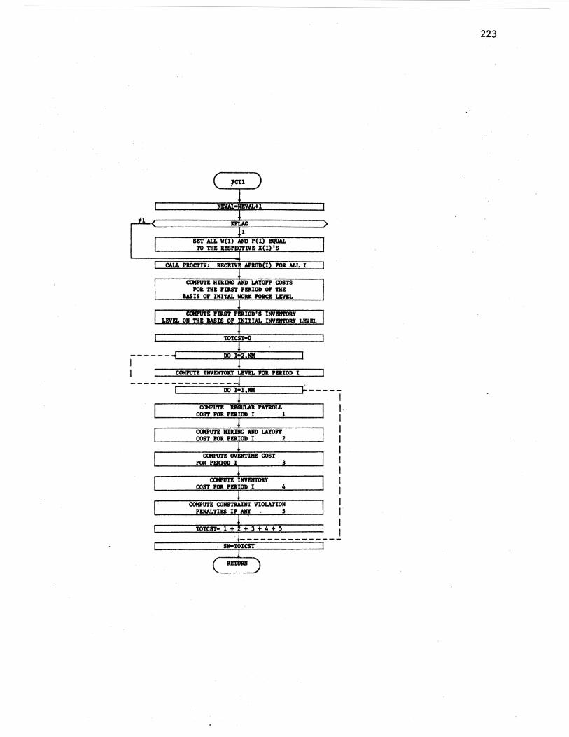
CALL PROCTIV: RECI'liV! APROD I POll ALL I

OIIIPUT! HIIll'IIG AIID LAYOFF COSTS POll Til! FIIST Pl!lliOD OF THE

BASIS OF IMITAL WORit POilC! LEVIL

CXIIPUTE FIIlST PDIOD S INVI!IITORY LEV!L ON THE BASIS OF INITIAL INVI!M'l'ORY LEV!L

caG'IIT! REGULAR PAYROLL COST POR PDIOD I 1

CXIG'UTE HIRING AIID LAYOFF COST POll Pl!lllOD I 2

CXIIPIJT! OVERTIME COST FOR PERIOD I 3

OIIIPUT! INVI!IITORY COST FOR PERIOD I 4

COMPUTE CONSTRAINT VIOLATION P!NALTII!S IF ANY 5

TOTCST-1+2+3+4+5

223

I I I I I I I I I I I I I I I I I I I I I I I I I I __ ----------

224

CHAMGED? X L+l 110

225

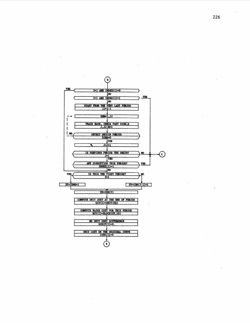
- ... I I I

YES

I HO r----===-==-=:::-:=:::-----,.

A!ff DlS'RUPTlON THIS PERIOD? YES DIDEX I •1

HO

IS THIS Til! FIRST P!IIOD?

226

227

COMPUTI THE liMIT COST AT 'lD !liD OF PERIOD

UC(J) • (1-J.(J)) •UKIT(UZ)+I.(J) •UKIT(UZN)

C<IIPUTE lll.lla COST POl THIS PEiiOD

BC(J) • (1-lt(J)) •l'l.OCa:(tl'l,UZ)+R(J) ·lll.lla(tmf,UZN)

------------1 I I I I I I I I

I I I

UC(It) - (1-R(K)) ·UC(It-l)+R(K) •UNIT(UZII) I I I

IIC(It)- (1-ll'(K))·BC(Jt-l)+l(lt)·BLOCit(UZl,UZN) I

----------------~

228

yea

I I I

IS THIS Till LAST PIRIOD1 I • .C

110

ADVAIICI I

IS DISIIIPTIOR TO II COHSIDIUD1 DLAG 2

COMPUTE PINAL PRODUCTIVITI!S FOR THIS VAJUAIILI S!T'l'OO

DO I • 1,101

I APROD(I) • P(I) /IICT(I) L_________ .

229

APPENDIX E

SEMI-DESCRIPTIVE FLOWCHARTS OF

COMPUTER PROGRAM FOR MODEL-II

230

231

( MAIN ) l

UAD PARAK!T!RS Or THE SEARCH IDUTIN!

l llEAD lfllllll!ll or P!lliODS l AIID DDIAND PER P!lliOD

! lU!AD STARTIRG VALUES, LOWER & UPPER BOUNDS FOR DECISION

VAIIABW

! READ PAIIAMBTilRS or THE

OBJECTIVE I'UMCTIOM

! READ THE SLOPES OF l LI!AIUIIING, PROOUSS AIID

FORGETTING CURVES

l lU!AD INITIAL CUKIILATIVE UIIIT l

IIIJKIID; IliiTIAL liOUl'ORCI LEVEL & IliiTIAL IliVEII'l'ORY L!VELS

! READ IlfiTIAL IIUIOIEit OF

EXPDIIIIICE CLASSIS, SIZI AIID PRODUCTIVITY HIASUU

or IACB CLASS

! COHPUTI EXPONENTS FOR

LIARNING, PMOGUSS & FORGETTING CURVIS

! COMPUTE THE OVDALL AVERAGE

PMODUCTIVITY FOR THE COliSTAliT PRODUCTIVITY )I)I)!L

cb

232

cp IallllC'fool: NO UnR!ltCI '10

CLASS

! CALL PATS: OPTIMIZE THE CONSTANT t-PRODUCTIVITY HODEL

IlfiTIALIZ! W (I) & P(I): CIJ!Alt II!FECT

l Iaiiuc:t-2; CALL FCTl 1-----< !VALUATE t1IE CONSTANT

PRODUCTIVITY HODEL

.----.j INITIALIZE W(I) & P(I): CLEAR I!F!CT

l 1 NEVAL-0

2 L CALL PATS: OPTIMIZE 'l'R!

DYNAMIC PRODUCTIVITY HODEL

! XDIRCT-3

t PRINT RESULTS I

! J KDIRCT 7. \.

~

233

( PCTl )

nvAL-rAL+l ltDIUCT

l SET ALL W{l) ' P~l) !QUAL TO THE USPECTIV! XCI) 'S

! CALL CLASS: UCEIV!

RIGIJI.Al TIME, OV!lTIMI!, AND IDL! li'ORICFOJ.CI LEVEL

AND SUBCOIITIACTIIIG QUAIITITY AND PI!NALTY CODES POll ALL PDIODS

! COMPUT! HIIliiiG AND LAYOPl

COSTS POl. THE PIJ.ST PDIOD 011 THE lAS IS OP THE

IIIITIAL WORICFOJ.CE LEVEL

~ TOTCST-0

COMPUTE IRV. LIV!LS POl. ALL PERIODS

I TOTCST- 1 + 2 + 3 + 4 + 5 + 6 I ------------:r I SJiooTOTCST

t

8

( CLASS

DIT!CT I!FCT, SET I•I!FECT

205)------------t·! ! • W I : W I-1 ~ >

SET THE TEMP. 110. OF CLASSIS .------,=-=:-!-!.....-.,-.,.,~---. INCREHEIIT or NIJMJIU or CLASSES NTIIIP-IfXCL(I-1)L-I __ WL-=:.!:W~I!:::-;;:.l>t..:•-:::W..l.(I~[)'---...J '----'NTEMP-=:::...::NX::yCL::=I:..--=1"--+'-'1,__ _ ___.

1 l l DO J•l NXCL I-1 !o- - -

rl DO -J•l,NTEKP I 1~--------~~--~~t=-~~~~==~~-, I ! K.•NXCLJI-1) I JET THE STATUS OF ALL

1 CLASSES BUT THE LAST 011! I SET THE TEMP. STATUS WTEIIP(J)•WXCL(I-l,J)

1 WTEKP<J>·wxCL<x-1 ,J> r -~ DO JJ·l 1: WTEMPCJ>·iJxcL<I-1 J)

I UTEMP(J)•UXCL(I-1,J) I 1 L-------~cb------~~r----~K~J~J~l~--~~s=ET~TIIE~S~U~TU~S~O=:r~TIIE~LAS~T~C~LAS~S~~

t---- -. -- B IIL..--===::::·:x,-1:+:::::=: I..-~=.~~~:::!------~ WTEIIP(NTEMP)•W(I)-W(I-1) UTEMP{JmHP)•O

I'---TL-:!..~~TL+WX=~CL~I!:::-.;!..1~J:.L--)-J 0 L ! = B ( !~ 1

SET 'Ill! TEMP. NO. Or CLASSES 1---'110""-P,_,All:=t;T::;IT;:I~ON"-;-"O~F-"A,_C,.,LA=SS><---; NT!MP•J 1'-I ___ .::NTEMP~r·;..::J~-~1---~

! r --- -l,__oo=-,JJ:;;;;•,_J--=1'---_,

I ! ~-~s!T==-=THE~=TEMP±=-.~S:TA~TUS==---, I lOR ALL CLASSES BUT THE LAST 011! I WT!HP(JJ)•WXCL(I-l,JJ) I UT!MP(JJ)•UXCL( I-1 JJ)

---------1 SET '1liE SIZE OF LAST CLASS

WT!KP(JJ •TL-WL

! SET '1liE PROD. MEASUil!

FOR 'Ill! LAST CLASS WT!KP(JJ

UTEMP (JJ)•(WXCL(I-l,JJ))

_ cucxib-L.JJj

DO JJ•l J-1

SET '1liE TEMP • STATUS POll ALL CLASSES

WTEKP(JJ).WXCL(I-1,JJ) UTEHP(JJ)•UXCL(I-1 JJl

234

235

l IMITALIZ! VALUIS FOR SUICOliTIACTIIIG

Allll COISTIAIIIT VIOLATIOII P!IIALTY PACTOltS FOR RI!KAIMIIIG PERIODS

SUI(l).O; PHALT(l).O

! UI.AG-0

! SET TH! IU!MAINIMG PROD.

!QUAL TO THE TOTAL PlOD. IR THE UP!CTIV! PERIOD

11'-P(I)

! COMPUTE UPP, THE PIOGUSS

FACTOR FOR THE BFP!CTIVE OMITS

! -----1 DO J•l, IIT!MP

! Ul•UTBMP(J)

! COMP,UTl! UGULAI. TIME

PlOD •. CAPABILITY OF EACH KEHlER 1M THI Jth CLASS

PCXR(I,J)•UPP*RIGPIO(Ul)

l UVISI IU'; PIIID TH!

EXCESS PlOD. AK!IIIIT

RP-~PCXR(I,J)•WTEHP(J)

.:o ! <0 c IU'

------------ --4>0 I COMPUTE TOTAL PlOD. IN REG. TIME J

PUG(I)•P(I)-IU' c

<b

IBCULAR TIM!, PlOD. ON OV!IlTIM! • llllll!ll OF

236

1------- ------ "----,.-....J

I I I I I I I I I I

COHPUT! 111! PlOD. CAPMILITY OF 111! J'nl CLASS 011 OYDTIME

Ul•UTIKP(J)+PCXR(I,J)/2 PCXO(l,J)•UPP.avRPIO(Ul)

UYIS! lP; COMPUTE THE !XC!SS PlOD. AMOUNT

RP-U-PCXO(l,J)*WT!MP(J)

I 1 u

~----------------- )a

S!T 111! MUHIIEJI. OF CLASSES

IIXCL(I)•MTEMP

~--- ------1 I UPDATI 111! STATUS OF I ALL CLASSES

I WXCL(I ,J)•WT!MP(J) UXCL(l,J)•UTEHP(J)+

I PCXR(l,J)+PCXO(I,J) !_ ____________ _

COMPUTE PI!IIALTY FACTOR; SIJBCOII­TIACTING AII>UIIT; UG. TIME ' OVDTIH! IIOIW'ORC! LEVEL lDl.!

IIORICFOitCE & PlOD. AII>UIIT IN OV!IlTIME

PHALT(I)•l; SUB(I)•IP WIII!G(I)•V(I); VOYa(I)•V(l)

VIDL(I)-<l POVIt(I)•P(I)-Pk!G(I)-lP

~.--------------------+1 1:101

237

1

TR! UHAilfiiiG CLASSES THAT AU lilT ASSIGDD OM

PIODUCTIOit o• OY!IlTIMI. Ill. OF Mill Olt UCULAR

TIMI AliD IDLE

238

APPENDIX F

FORTRAN PROGRAM LISTINGS

239

000.10 c 00020 c 00030 c 00040 c oooso c 00060 c 00070 c 00080 c 00090 c 00100 c 00110 c 00120 c 00130 c 00140 c 00150 c 00160 c 00170 c 00180 c 00190 c 00200 c 00210 c 00220 c 00230 c 00240 c 00250 c oo26o ·c 00270 c 00280 00290 00300 00310 00320 00330 00340 00350 00360 00370 00380 c

FORTRAN CODES FOR AGGREGATE PLANNING MODELS WITH DYNAMIC PRODUCTIVITY

PROGRAMMED BY B. KHDSHNEVIS

APRIL 1979

***************************** * * * H A I N P R 0 G R A H * * * * F 0 R H 0 D E L -I * * * *****************************

FORTRAN CODE FOR AGGREGATE PLANNING OF LONG CYCLE PRODUCTS

IMPLICIT REAL*8 CA-HrO-Z> COMMON /SHARE/ X<20)rNrNMrSN COMMON /SRCHP/ XMAXC20>rXMINC20)rLIMrKPRESSrNO COMMON /VALUE/ NEVAL COMMON /PRODY/ UCTC20)rBCTC20)riCHKC20)riNDEXC20>rRC20)r

1CUMOrTRSHLJEPSYrAK1rAK2rAK3rZADJ COMMON /THREE/ WC20)rPC20>rAPRODC20>rWOrKFLAG COMMON /OBJFN/ DC20)~DPCS7C20>rHLCSTC20)r0VCSTC20>rDINVC20)r

1STCSTC20>rTCC20>rOINVrTOTCSTrC1rC2rC3rC4rC5rC6rC7rC8rC9rC10 COMMON /CURVE/ BrF

00390 C SET THE INPUT-OUTPUT UNIT NUMBERS 00400 IN=S 00410 N0=6 00420 C READ IN THE MASTER CONTROL DATA - SEE GLOSSARY FOR DEFINITIONS 00430 READ<INr1>KPRESSrLIMrNM 00440 N=2*NM 00450 C READ IN THE MONTHLY DEMAND LEVELS 00460 READ<INr2) CD<I>ri=1rNM> 00470 C READ IN THE INITIALr STARTING VALUES FOR THE DECISION VARIABLES 00480 C PRODUCTION RATES AND WORKFORCE LEVELS 00490 READCINr3> CX<I>ri=1rN> 00500 C READ IN THE UPPER AND LOWER LIMITS FOR DECISION VARIABLES 00510 DO 10 I=1rN 00520 10 READ<INr4) XMAXCI>rXMIN<I>

240

00530 C READ IN THE VALUES OF THE COST PARAMETERS IN THE OBJECTIVE FUNCTION 00540 READCINrS> C1rC2rC3rC4rC5rC6rC7rC8rC9rC10 00550.C READ IN THE PARAMETERS OF THE IMPROVEMENT CURVE 00560. READCINr6)~SrF

0057o·c READ IN THE PARAMETERS OF MANPOWER CHANGE DISRUPTIONS AND 00580'-:t: -coMPOUNDED II!SRUPTION EFFECTS 00590 READCINr7) AK1rAK2rAK3rTRSHLrEPSY 00600 C READ IN THE INITIAL CUMULATIVE UNIT NUMBERriNITIAL WORKFORCE 00610 C AND INITIAL INVENTORY LEVELS 00620 READCINr8> CUMOrWOrDINV

00630 c 00640 00650 00660 c

COMPUTE THE EXPONENT VALUE OF THE IMPROVEMENT CURVE Tlol0=2.

-00670 -~00680 ,' -oo690 _ -too

00700

B=-DLOGCS)/DLOGCTWO)

DO 100 I=ltNM INDEX <I >=O ICHK CI >=0

,=--KFLAG=1 C "-COMPUTE --THE- OVERALL AVERAGE..:RRODUCTIVITY- ON THE BASIS OF THE -- 00710

oono 00730 00740 00750 00760 00770 00780 200 00790 00800 00810 00820 c 00830 c 00840 c 00850 00860 00870 c 00880 c 00890 00900 00910 00920 00930 00940 c 00950 c 00960 c 00970 00980 00990 01000 c 01010 c 01020 01030 01040 c 01050 c 01060 c 01070 01080 01090 01100 01110 01120 01130 01140 01150 c 01160 c 01170 01180 01190 01200 01210 01220 01230 01240 c 01250 c 01260 c 01270

C TOTALDEHAND• THE INITIAL. CUMULATIVE UNIT~NUMBERAND THE GURRENT C IMPROVEMENT CURVE PARAMETERS--PURPOSE: TO BE USED FOR EVALUATION C OF THE CONSTANT PRODUCTIVITY MODEL c

TDND=O. DO 200 I=1•NH TDND=TDND+D<I> T=TDNDtCUHO THHR=BLOCK<CUHO•T> CAPR=TDND/TNHR

SET THE AVERAGE MONTHLY PRODUCTIVITY LEVELS EQUAL TO THE CONSTANT, OVERALL AVERAGE PRODUCTIVITY LEVEL

DO 300 I=l•NM 300 APRODCI>=CAPR

OPTIMIZE THE CALL PATS KPRINT=1

. GO TO 800 701 KFLAG=O

KPRINT=2

CONSTANT PRODUCTIVITY HODEL AND PRINT THE RESULTS

INITIALIZE THE DECISION VARIABLES TO CLEAR 'IEFECT' --THE COPY OF THE ORIGINAL VALUES IS SAVED IN XC.>

DO 400 I=lrNH W<I >=O.

400 P<I>=O. EVALUATE THE RESULTS OF THE CONSTANT PRODUCTIVITY HODEL BY AN INDIRECT CALL TO 'PROCTV' rTHROUGH 'FCT1' , -PRINT THE RESULTS

CALL FCTl GO TO 800

SUPPRESS THE EFFECT OF MANPOWER DISRUPTIONriNITIALrzE VARIABI:.ES AND OPTIMIZE THE 'EBERT' MODEL--PRINT THE RESULTS

702 KFLAG=2 KPRINT=3 DO 500 I=1tNH W<I>=O.

500 PCI>=O. NEVAL=O CALL PATS GO TO 800

EVALUATE THE RESULTS OF OPTIMIZATION OF THE EBERT HODEL--PRINT RESULT 703 KFLAG=O

KPRINT=4 DO 600 I=lrNH W(!)=O,

600 P<I>=O. CALL FCTl GO TO 800

PUT THE DISRUPTION BACK TO EFFECT AND OPTIMIZE THE DYNAMIC PRODUCTIVITY HODEL - PRINT THE RESULTS

704 KPRINT=5

241

01280 01290 01300 01310 01320

DO 700 I=1rNI1 W<I>=O•

700 PCI>=O. NEVAL=O CALL PATS

-'I01330 .c. 01340

800 DO 900 I=1rNH - 900 ~RITEfN0~1000) IrDCilrWCI>rPCI>rDINV<I>rAPRODCI>~INDEXCI)iiCHKCI)

01350 c .:.~01360

01370 01380 c 01390 c 01400 01410 c 01420 01430 01440 01450 01460 01470 01480 01490 01500 01510

-DO 91v I:.:1 rNH 910 WRITECNOr1001)

WRITECN0.1002> IrDPCST<I>rHLCST<I>rOVCSTti)rSTCST<I>~TCCI> TOTCST

DIRECT THE CONTROL TO THE PROPER STAGE IN THE ABOVE SEQUENCE GO TO C701r702r703r704,999)rKPRINT

1 2 3 4 5 6 7 8

1000 1001

FORMAT<3I5> FORHATCSX, FlO • 0) FORHAT<F10.0> FORMATC5Xr2F10.0> FORMAT< 10F8.3> FORMATC5XrF5.4rF10.3) FORMATC5F10.S> FORMATC5Xr3F10.0> FORMATC1Xri2r2Xr4CF5.1r2X>rF10.3r2Xr2CI2r2X)) FORMATCBXrl2rSCF11.2r2X))

01520 1002 01530 999 01:540

FORMATC35XrF10.2> STOP END

01550 c (J 01560 c

01:570 c~ 01580 c 01590 c 01600 c 01610 c 01620 c 01630 c 01640 c 01650

********************************* * * * OBJECTIVE FUNCTION SUBROUTINE *

01660 c 01670 c 0168o·c 01690 c

. 01700 c 01710 01720 01730 01740 01750 01760 01770 c 01780 01790 c 01800 c 01810 c 01820 c 01830 c 01940 01850 01860 01970 01880 01990 01900 01910 01920

* * *********************************

SUBROUTINE FCT1

THIS ROUTINE EVALUATES THE-RESPONSE OF THE COST FUNCTIO~ AGAINST THE VALUES OF THE-DECISION VARIABLEScAND AVERAGE PRODUCTIIJITYLEVELS RECEIVED EITHER FROM THE· MAIN PROGRAM OR THE PATTERN SEARCH ~NE •

IMPLICIT REAL*B <A-H,O-Z> COMMON /SHARE/ XC20)rNrNMrSN COMMON /VALUE/ NEVAL COMMON /THREE/ WC20)rPC20>rAPRODC20)rWOrKFLAG COMMON /OBJFN/ DC20>rDPCSTC20)rHLCSTC20)r0VCSTC20>rDINVC20)r

1STCSTC20>rTCC20>rOINVrTOTCSTrClrC2rC3rC4rCSrC6rC7rC8rC9rC10 INCREMENT THE NUMBER OF OBJECTIVE FUNCTION EVALUATIONS

NEVAL=NEVAL+1 THE FOLLOWING STH DIRECTS THE CONTROL TO EVALUATION OF EITHER CONSTANT PRODUCTIVITY; OR EBERT AND DYNAMIC PRODUCTIVITY MODELS. THE VALUES OF THE DECISION VARIABLES ARE FIRST SET FOR EVALUATION OF THE CONSTANT PRODUCTIVITY MODEL

100

IF<KFLAG.NE .1)

...1=0 K=N-1 DO 100 L=1rKr2 .J=J+1 WCJ>=X<L> P<J>=XCL+U CONTINUE GO TO 300

GO TO 200

242

01930 c 01940 c 01950 c 01960 01970 c 01980 01990 02000 02010 02020 02030 02040 02050 02060 02070 02080 c 02090 02100 02110 02120 02130 02140 c 02150 c 02160 02170 02180 02190 c 02200 c 02210 c 02220 c 02230 c 02240 c 02250 c 02260 c 02270 c 02280 c 02290 02300 c 02310 c 02320 c 02330 c 02340 c 02350 02360 02370 02380 02390 02400 02410 02420 c 02430 c 02440 c 02450 c 02460 02470 02480 02490 02500 02510:-"-02520 02530 02540 02550

.02560 02570

RECEIVE THE MONTHLY LEVELS OF THE AVERAGE PRODUCTIVITIES ASSOCIATED ASSOCIATED WITH THE CURRENT DESICION -- "PROCTV" PROVIDES THIS

200 CALL PROCTV COMPUTE MONTHLY AND TOTAL COSTS RELATED TO THE CURRENT DESICION

300 TOTCST=O. HLCST<1>=C2*(W(1)-W0>**2 DINV<1>=P<1>+DINV-DC1> DO 400 I,;2rNM

400 DINV<I>=P<I>tDINV<I-1>-DCI) DO 500 I=1rNM . DPCSTCI>=CUW<I> IFCI.NE.1> HLCST<I>=C2*<W<I>-W<I-1>>**2 OVCST<I>=C3*<P<I>-APROD<I>*W<I>>**2+C5*P<I>-C6*W<I> STCST<I>=C7*<DINV<I>-C8>**2

INCORPORATE THE PENALTY FOR CONSTRAINT VIOLATION IF<DINV<I>.GT.900) PNLT=100000. PNLT=O. TC<I>=DPCST<I>tHLCST<I>tOVCSTCI>+STCST<I>+PNLT TOTCST=TOTCST+TC<I>

500 CONTINUE

DIRECT THE THE RESPONSE LEVEL TO THE CALLING ROUTINE SN=TOTCST RETURN END

************************

* * * DYNAMIC PRODUCTIVITY * * SUBROUTINE * * * ************************

SUBROUTINE PROCTV

THIS ROUTINE COMPUTES THE MONTHLY AVERAGE PRODUCTIVITY LEVELS FOR ANY SET OF DECISION VARIABLES RECEIVED FROM THE CALLING ROUTINE. <SEE THE GLOSSARY FOR VARIABLE DEFINITIONS; AND RELATED FLOW-CHARTS)

IMPLICIT REAL*B <A-HrO-Z> DIMENSION CUMC20)rTNMPC20)rUCC20)rBCC20)rUCDIFC20)rUCDRC20) COMMON /SHARE/ XC20>rNrNMrSN COMMON /PRODY/ UCTC20)rBCTC20)riCHK<20>riNDEXC20>rRC20)r

1CUMOrTRSHLrEPSYrAK1rAK2rAK3rZADJ COMMON /THREE/ WC20>rPC20>rAPRODC20>rWOrKFLAG COMMON /CURVE/ BrF

THE FOL~OWING STNS· CTHRU STM·200t1) DETECT THE EFFECTIVE PERIOD AT WHICH THE FIRST CHANGE IN THE LEVEL OF A DECISION VARIABLE IS MADE BY THE SEARCH ROUTINE

ICNTRL=1 J=O IP=1 I<=N-'1 DO 200 L=l rl<r2· · J=J+l IF{W(J)-XCLll 120r110r12~ ~

120 W(J)=X<L> GO TO <130rl10)riCNTRL

130 ICNTRL=2 IEFCT=J

110 IF(P(J)-X(Lt1)) 140r100,140

243

J

02580 02590 02600 02610

- 02620 .:. 02630 .:~02640 - '02650 ~02660

c

140 PCJ>=XCLH> IP=2

100 GO TO C200r145>riP 145 IFCJ-1> 160r150r160 150 PCUH=CUI'IO

·:~GO TO 170 =160-PCUH=CUHCJ-1) 170 CUHCJ>=PCUHtPCJ>

GO TO C180r200>riCNTRL 180 ICNTRL=2

IEFCT=J 200 CONTINUE

I=IEFCT

244

C DIRECT THE CONTROL TO COMPUTATION OF AVERAGE PRODUCTIVITIES FOR C EITHER EBERT OR DYNAMIC PRODUCTIVITY MODELS

02670 02680 02690 02700 02710 02720 02730 02740 02750 02760 02770 02780 c 02790 c 02800 c 02810 02820 02830 02840 02850 02860 02870 c

c

IF<KFLAG.ED.2> GO TO 380 IFCI-1> 300r250r300

250 WOLD=WO GO TO 350

COMPUTE THE UNDELUTED IN THE CURRENT PERIOD

300 350

WOLD=W C I -1> ADJ=ZADJ

MANPOWER TUNOVER RATIO FOR THE MANPOWER LEVEL -- CHECK THE SIGNIFICANCE OF DISRUPTION

IFCI~NE.1> ADJ=O. TNMPCI>=CDABSCWCI>-WOLD>>IDMAX1CWCI)rWOLD> IFCTNMPCl).LE.TRSHL>GO TO 380 INDEXCI>::;:,t

CHECK FOR MANPOWER REDUCTION OR ADDITION -- DELUTE THE TURNOVER RATIO IFCW<I>.LT.WOLD)GO TO 370 RCI>=AK1*CTNMPCI>-AK2>+ADJ GO TO 400

370 RCI>=AK1*CAK3*TNMPCI>-AK2>+ADJ GO TO 400

380 INDEXCI>=O

02880 02890 02900 02910 02920 02930 02940 02950 02960 02970 02980

400 IF<I.ED,f< AND•-INDEX<I >, EQ. 0 > IFCI.EG.1.AND.INDEXCI>.EG.1)

C TRACE BACK FOR DETECTION OF THE C DISRUPTION

GO TO 600 GO TO 650 ORIGINATION OF TH~COMPOUNDED

-. 02990 03000

.03010 03020 03030 03040 03050 03060 03070 03080 03090 03100 03110 03120 c 03130 c 03140 c 03150 03160 c 03170 03180 c 03190 c 03200 c 03210 03220

JJ=I-1 DO 500 M=1rJJ J=JJ-MH IFCICHKCJ>> 500r550r~OO

500 CONTINUE 550 J=JH

IFCI-J> 700r590r700 590 IFCINDEXCI>> 650r600r650 6QO 610

620 640

IFCI-1> 620r610r620 UY=CUMOH • -GO TO 640 UY=CUMC I-1 >t1. UZ=CUMCI>

NO DISRUPTION -- COMPUTE THE UNIT COST AT THE END OF THE PERIOD CON THE ORIGINAL CURVE>

UCTC I >=UNIT<UZ> COMPUTE THE BLOCK COST OF THE CURRENT PERIODCON ORIGINAL CURVE>

BCTCI>=BLOCKCUYrUZ> SET THE UNIT COST DIFFERENCE AT THE END Of THIS PERIOD EQUAL TO ZEROr BECAUSE NO DISRUPTION HAS OCCURED AND THERE IS NO CONTINUING EFFECT OF THE PREVIOUS ONESCIF ANY)

UCDR c-I > =0. I CHI(( I >=O

03230 03240-C 03250 c 03260 c 03270

---03280 <·.;.03290 --;03300

03310 ,- 03320

c

245

GO TO 900

STMS 650 THRU 730t4 COMPUTE THE SINGLE DISRUPTION EFFECT OCCURING AT THE BEGINNING OF THE CURRENT PERIOD

650 J:~~I

700 IF< I-1) 720r710r720 710-UY=r·~MOU.

. UX=UY-1. GO TO 730

720 UY=CUMCI-1>+1. UX=CUM<J-1)

730 UZ=CUMCI> UZN=UZ-UX UYN=UY-UX UCCJ>=C1.-RCJ>>*UNITCUZ>tR<J>*UNITCUZN> BC<J>=C1.-RCJ>>*BLOCKCUYrUZ>+R<J>*BLOCKCUYNrUZN>

C FOLLOWING STMS <THRU STM 850t4> DETERMINE THE COMPOUNDED DISRUPTION C EFFECT FOR THE CURRENT PERIOD THROUGH RECURSIVE COMPUTATIONS.

03330 03340 03350 03360 03370 03380 03390 03400 03410 03420 03430 03440 03450 03460 03470 03480 03490 03500 03510 03520 03530 03540 03550 03560 03570 03580 03590 c 03600 c 03610 03620 03630 03640 03650 03660 c

. 03670 03680 03690 03700 c 03710 c 03720 c 03730 03740 03750 03760

. 03770

c c

IFCI-J> 740r850r740 740 JJ=J+1 .

DO 800 K=JJri IFCINDEXCK>> 765r755r765

755 UCCK>=UCCK-1> BCCK>=BCCK-1> GO TO 800

765 UX=CUM<K-1> UZN=UZ-UX UZY=UY-UX UC<K>=<1.-RCK>>*UCCK-1>+R<K>*UNIT<UZN> BCCK>=C1.-RCK>>*BCCK-1>+RCK>*BLOCKCUZYrUZN>

BOO CONTINUE 850 UCTC I > =UC ( I >

BCTCI>=BCCI> UCDIF<I>=UCT<I>-UNITCUZ> UCDR<I>=UCDIF<I>/CUCT<I>>

CHECK TO SEE IF THE DISRUPTION EFFECT CARRIED OVERTHE NEXT PERIOD IS SIGNIFICANT

IFCUCDR<I>.LE.EPSY> GO TO 870 ICHK<I>=1 GO TO 900

870 ICHKCI>=O 900 IFCI.EQ.NM> GO T~ 999

INCREMENT THE PERIOD NUMBER -- REPEAT THE PROCESS FOR THE NEXT PERIOD I=It1 IFCKFLAG.EG.2> GO TO 380 GO TO 300

COMPUTE THE FINAL VALUES OF THE MONTHLY AVERAGE DIRECT THE VALUES TO THE CALLING ROUTINE

999 DO 1000 I=IEFCToNM 1000 APRODCI>=PCI)/CBCTCI>>

ZADJ=UCDRC1> RETURN END

**************** FUNCTION UNIT<UA> ****************

PRODUCTIVITY LEVELS-

03780 c 03790 c 03800 c 03810 03820 03830 03840 03850 03860 03870

C THIS FUNCTION COMPUTES THE UNIT COST FOR ANY CUMULATIVE UNIT NUMBER c

IMPLICIT REAL*B CA-HrO-Z> COMMON /CURVE/ BrF

03880 03890 03900 03910 03920 03930 03940 c

=-.03950 c --:03960 c ·-03970

03980 c 03990 c 04000 c 04010 c 04020 04030 04040 04050 0-4060 04070 04080 04090 04100

IF(CUA**B>.LT.1) GO TO 1 UNIT=F / <UAUB) RETURN

1 UNIT=F RETURN

·c END

******************** -FUNCTION BLOCKfUArUB>

******************** THIS FUNCTION COMPUTES THE UNIT COST FOR ANY RANGE OF CUMULATIVE UNIT NUMBERS r UA THRU UB

IMPLICIT REAL*B CA-HrO-Z) COHMO~~/CURVE/ B,F IFCUA-UB> 2r 1r 2

1 BLOCK=O RETURN

2 BLOCK=<FIC1.-B>>*<<UB+.S>**C1.-B>-<UA-.5>**<1.-B>> RETURN END SUBROUTINE PATS

246

00010 c ~:.00020 c ;C;;;00030 c ~\00040 c ~-ooo5o c ~o~o6o c ·ooo.1o c 00080 c 00090 c 00100 c 00110 c 00120 c 00130 c 00140 c 00150 c 00160 00170 00180 00190 00200 00210 00220 00230 00240 00250

ll 00260 00270 00280 00290 00300 c 00310 00320 00330 c 00340 00350 00360 c 00370 00380 c 00390 00400 c 00410 00420 00430 c 00440 00450 c 00460 c 00470 00480 c 00490 00500 00510 c 00520 c 00530 00540 00550 c .00560 c 00570 00580 c 00590 00600 00610 00620

***************************** - * * = *~ K A I N c P R O·G R A H * * * * ~ F 0 R H 0 D E L-II * * * *****************************

FORTRAN CODE FOR AGGREGATE PLANNING OF SHORT CYCLE PRODUCTS

IMPLICIT REAL*8 <A-HrO-Z> COMMON /SHARE/ X<40>rNrNHrSN COMMON /SRCHP/ XMAX<20>rXMINC20)rLIMrKPRESSrNO COMMON /VALUE/ NEVAL COMMON /CCLSS/ NXCLC20)rWXCLC20r50>rWXCLOC10)rUXCLOC10)rCUMO

1rNXCLO COMMON /THREE/ WC20)rPC20>rWREGC20>rWOVRC20>rWIDLC20)r

1PREGC20>rPOVRC20>rSUBC20>rPNALTC20)rWO COMMON /OBJFN/ D<20)rDPCSTC20>rHLCSTC20>rOVCST<20>rDINVC20)r

1STCST<20>rOINVrTOTCSTrC1rC2rC3rC4rC5rC6,C7rC8rC9rC10,KDIRCT COMMON /LEARN/ B,F COMMON /PROGS/ BP COMMON /FORGT/ BFrF1 COMMON /OVPCT/ OPCNT

SET THE INPUT-OUTPUT UNIT NUMBE~ NI=5 N0=6

READ IN THE MASTER CONTROL DATA - SEE GLOSSARY FOR DEFINITIONS READ<INrl)_KPRESSrLIMrNM N=2*NM

READ IN THE MONTHLY DEMAND LEVELS READCINr2) CDCI>ri=1rNM>

.READ IN THE INITIALr- STARTING --VALUEs- FOR THE- DECISION VARIABLES READ<INr3) <X<I>ri=1rN>

READ IN THE UPPER AND THE LOWER LIMITS ON THE DECISION VARIABLES DO 10 I=1rN

10 READ<INr4) XMAX<I>•XMINCI>

247

READ IN THE VALUES OF THE COST PARAMETERS IN THE OBJECTIVE FUNCTION READCINr5) C1rC2rC3rC4rC5,C6,C7rC8rC9,C10

READ IN THE INITIAL NUMBER OF EXPERIENCE CLASSESriNITIAL CUMULATIVE OUTPUT UNIT NUMBERr AND INITIAL INVENTORY LEVEL

READCINr6> NXCLOrCUMO,OINV READ IN THE SIZE AND PRODUCTIVITY MEASURE OF EACH INITIAL CLASS

DO 20 I=lrNXCLO 20 READCINr7> WXCLO<I)rUXCLOCI> READ IN THE SLOPES OF LEARNING• PROGRESS, AND-FORGETTING CURVES ;AND THE BASE UNIT COST

READ<INr8) SLrSPrSF,F Fl=F

READ IN THE LENGTH OF OVERTIME WORK AS A PERCENTAGE OF THE REGULAR TIME WORK

READCINr9> OPCNT COMPUTE THE EXPONENT VALUES FOR THE THREE CURVES

TW0=2. B=-D~OGCSL)/DLOG<TWO> BP=-DLOGCSP)/DLOG<TWO> BF=-DLOG<SF)/DLOGCTWO>

00630 c 00640 00650 00660

-'--00670 c

COMPUTE THE TOTAL INITIAL WO=O. DO 100 I=lrNXCLO

100 WO=WOtWXCLO(I)

248

MANPOWER LEVEL

·J" 0068.0 C · COMPUTE SLOPE AND ·EXPONENT OF. THE OVERALL- IMPROVEMENT CURVE, AND ON -~· 00690 C "·c,THE BA~!S OF~ THIS CURVE AND. THE. TOTAL DEMAND'i• COMPUTE:'-·THE·'·OVERALL

,:_ -00700 C·' AVERAGECCONSTANT>-E'RODUCTIVITY LEVEL -- I?URPOSEi'TO. BE USED IN THE 00710 C EVALUATION OF THE CONSTANT PRODUCTIVITY MODEL

- 00720 c 00730 00740 00750 00760 00770 00780 00790 00800 00810 00820 00830 c 00840 00850 00860 c 00870 c 00880 00890 00900 00910 00920 c

SS=SL*SP BC=-DLOGCSS)/DLOGCTWO) TDND=O. DO 150 .I=lrNM

150 TDND=TDND+D<I> T=CUMO+TDND THHR=CF/(1.-BC>>*<<Tt.5>**<1.-BC>-<CUH0-~5>**<1.-BC)) C4:o:TDNDITHHR KDIRCT=1 NEVAL=O

OPTIMIZE THE CONSTANT CALL PATS GO TO 450

PRODUCTIVITY HODEL -- PRINT THE RESULTS

INITIALIZE THE DECISION VARIABLES TO CLEAR IEFCT - A COPY OF THE ORIGINAL VALUES IS SAVED IN XC.>

250 DO 300 I=1rNH W<I>=O

300 P<I>=Oo KDIRCT=2

00930 C EVALUATE THE RESULTS OF THE CONSTANT PRODUCTIVITY HODEL BY AN 00940 C INDIRECT CALL TO 'CLASS'• THROUGH 'FCT1'--PRINT THE RESULS 00950 CALL FCT1 . 00960 GO TO 550 00970 C INITIALIZE THE DECISION VARIABLES AND OPTIMIZE THE DYNAMIC 00980 C PRODUCTIVITY MODEL -- PRINT THE RESULTS 00990 350 DO 400 I=1rNH

·01000 W<I>=O. 01010 400 P<I>=O. 01020 NEVAL=O

--01030 .. CALL P-.ATS 01040 KDIRCT=3 01050 GO TO 550 01060 450 DO 500 I=lrNM 01070 500 WRITECNOr1000) IrD<I>rWCI>rPCI>rWOVR<I>rWIDL<I>rSUBCI> 01080 GO TO 700 01090 550 DO 600 I=1rNM 01100 600 WRITECN0r1001) IrD<I>rWCI>rP<I>rDINVCI>rWREG<I>rWOVRCI)r 01110 1WIDL<I>rPREG<I>rPOVR<I>rSUB<I> 01120 DO 650 I=1rNH 01130 SUCST=C10*SUB<I> 01140 650 WRITE<NOr1003) IrDPCSTCI>rHLCSTCI)rOVCSTCI>rSTCSTCI>rSUCST 01150 700 WRITE<NOr1002> TOTCST 01160 c. 01170 c 01180 01190 c 01200 01210 01220 01230 01240 01250 01260 01270

DIRECT THE CONTROL TO THE PROPER STAGE IN THE ABOVE SEQUENCE GO TO C250r350r999)rKDIRCT

1 FORHAT<3IS> 2 FORHATC5XrF10.0) 3 FORHATCF10.0) 4 FORHAT<5Xr2F10.0) 5 FORHATC10F8.3> 6 FORHATCSXri5r2F10.0) 7 FORHATC2F5.0) 8 FORHAT<5Xr3F5.4rF10.3)

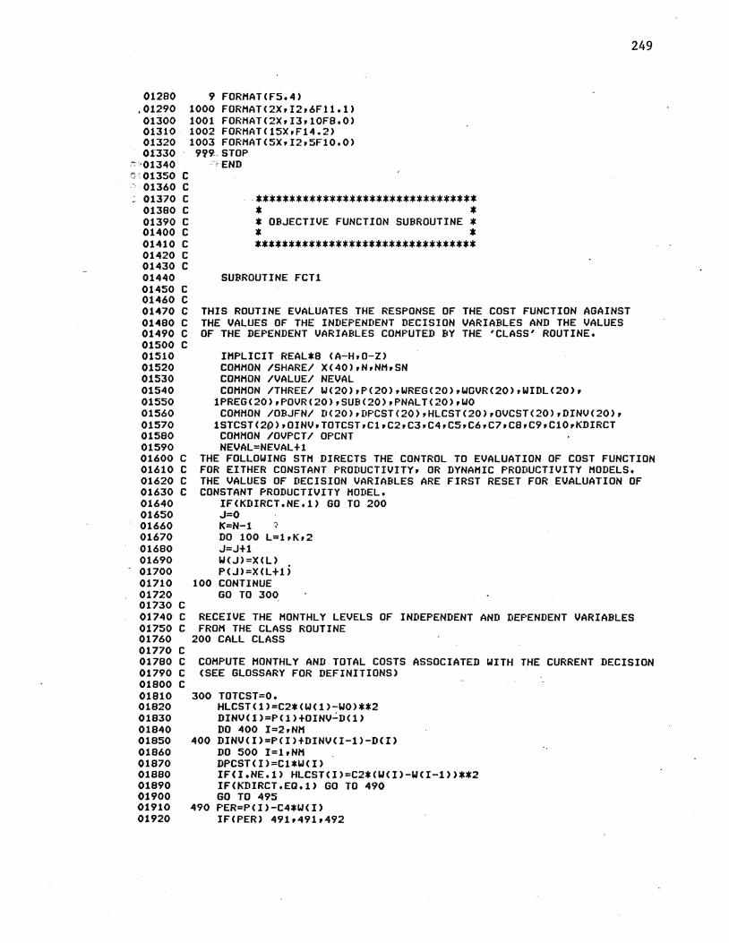
01280 .01290 01300 01310 01320 0-1330

,>01340 01350 c 01360 c

- 01370 c 01380 c 01390 c 01400 c 01410 c 01420 c 01430 c 01440 01450 c 01460 c 01470 c 01480 c 01490 c 01500 c 01510 01520 01530 01540 01550 01560 01570 01580 01590 01600 c 01610 c 01620 c 01630 c 01640 01650 01660 01670 01680 01690

- 01700 01710 01720 01730 c 01740 c 01750 c 01760 01770 c 01780 c 01790 c 01800 c 01810 01820 01830 01840 01850 01860 01870 01880 01890 01900 01910 01920

9 FORMAT< F5. 4) 1000 FORMAT<2Xri2r6F11.1) 1001 FORMAT<2X,I3,10F8.0) 1002 FORMAT<15XrF14.2) 1003 FORMATC5Xri2r5F10.0>

99SLSTOP -,c END

*********************************

* * * OBJECTIVE FUNCTION SUBROUTINE *

* * *********************************

SUBROUTINE FCT1

THIS ROUTINE EVALUATES THE RESPONSE OF THE COST FUNCTION AGAINST THE VALUES OF THE INDEPENDENT DECISION VARIABLES AND THE VALUES OF THE DEPENDENT VARIABLES COMPUTED BY THE 'CLASS' ROUTINE.

IMPLICIT REAL*8 <A-HrO-Z> COMMON /SHARE/ XC40)rNrNMrSN COMMON /VALUE/ NEVAL COMMON /THREE/ W<20>rP<20>rWREGC20)rWOVRC20>rWIDL<20)r

1PREG(20>,POVRC20)rSUBC20)rPNALTC20)rWO COMMON /OBJFN/ D<20>rDPCSTC20)rHLCST<20>rOVCST(20),DINVC20),

1STCST(20>rOINV•TOTCSTrC1rC2rC3rC4rC5rC6rC7rC8rC9rC10rKDIRCT COMMON /OVPCT/ OPCNT NEVAL=NEVAL+l

249

THE FOLLOWING STM DIRECTS THE CONTROL TO EVALUATION OF COST FUNCTION FOR EITHER CONSTANT PRODUCTIVITY• OR DYNAMIC PRODUCTIVITY MODELS. THE VALUES OF DECISION VARIABLES ARE FIRST RESET FOR E~ALUATION OF CONSTANT PRODUCTIVITY MODEL.

IF<KDIRCT.NE.1) GO TO 200 J=O K=N-1 ~

DO 100 L=lrKr2 J=J+l W<J>=X<L> P<J>=X<L+l)

100 CONTINUE GO TO 300

RECEIVE THE MONTHLY LEVELS OF INDEPENDENT AND DEPENDENT VARIABLES FROM THE CLASS ROUTINE

200 CALL CLASS

COMPUTE MONTHLY AND TOTAL COSTS ASSOCIATED WITH THE CURRENT DECISION <SEE GLOSSARY FOR DEFINITIONS>

300 TOTCST=O, HLCST<1>=C2*<W<1>-W0>**2 DINV(1)=P<l>+OINV~D<1> DO 400 I=2rNM

400 DINV<I>=PCI>+DINV(I-1>-D<I> DO 500 I=l•NH DPCST<I>=Cl*W<I> IFCI.NE.1> HLCST<I>=C2*<W<I>-W<I-1>>**2 IF<KDIRCT.EQ.l> GO TO 490 GO TO 495

490 PER=P<I>-C4*W<I> IF<PER> 491,491o492

01930 01940· 01950 01960 01970

=--~1980 ::;~01990 ~::'02000 ::-,-:02010 :.:.02020

491 WOVRCI>=Oo SUBCI>=O. WIDL<I>=-PER/C4 GO TO 495

492 SB=PER-OPCNT*C4*W<I> IFCSB) 493~493i494

~-493~WOVRCI>=PER/COPCNT*C4J SUBCI)=O,

~GO TO 495 ~ 494-WOVR <I l=W< I>.

SUBCI>=SB WIIIL<I>=O.

495 OVCSTCI>=Cl*WOVRCI> STCST<I>=C7*<DINVCI>-CB>**2 TOTCST=TOTCSTtDPCST<I>+HLCSTCI>+OVCST<I>tSTtST<I>tC10*SUB<I>

~tC3*CPCI>-C5>**2 500 CONTINUE

DIRECT THE RESPONSE SN=TOTCST

LEVEL TO THE CALLING ROUTINE

RETURN END

************************

* * * DYNAMIC PRODUCTIVITY * * SUBROUTINE *

* * ************************

SUBROUTINE CLASS

250

02030 02040 02050 02060 02070 02080 02090 02100 c 02110 c 02120 02130 02140 02150 c 02160 c 02170 c 02180 c 02190 c 02200 c 02210 c 02220 c 02230 c 02240 c 02250 c 02260 02270 c 02280 c 02290 c

-~02300 c 02310 c 02320 c 02330 c 02340

THIS ROUTINE COMPUTES THE MONTHLY LEVELS OF THE DEPENDENT DECISION JlARIABLES AND THE STATUS OE EXPERIENCE Ct.ASSES FOR AN'CSEr OF INDEPENDENT DECISION VARIABLES RECEIVED FROM THE CALLING ROUTINE. CSEE GLOSSARY FOR VARIABLE DEFINITIONS AND THE RELATED FLOWW-CHARTS>

. ~02350 02360 02370 02380 02390 02400 02410 02420 02430 02440 02450 02460 02-470 c 02480 c 02490 c 02500 c 02510 02520 02530 02540 02550 02560 02570

IMPLICIT REAL*B <A-HrO-Z> - DIMENSION. CUM-<20> O:WXXC50) rUXXC50) rWTEMPC50hUTEMPCSO>, 1PCXRC20rSO>rPCX0<20r50>rUXCL<20r50)

COMMON /SHARE/ XC40>rNrNMrSN COMMON /CCLSS/ NXCL<20>rWXCLC20rSO>rWXCLOC10>rUXCLOC10>rCUMO

lrNXCLO COMMON /THREE/ WC20)rPC20)rWREGC20>rWOVRC20>rWIDLC20)r

1PREGC20)rPOVRC20)rSUBC20)rPNALTC20)rWO COMMON /LEARN/ ElrF COMMON /PROGS/ BP COMMON /FORGT/ BFrFl COMMON /OVPCT/ OPCNT TOL=l.

THE FOLLOWING STMS AT WHICH THE FIRST MADE BY THE SEARCH

ICNTRL=l IP=l .J=O K=2*NM-1 DO 200 L=lrKr2 .J=.Jtl

CTHRU STM 200t1> DETECT THE EFFECTIVE PERIOD CHANGE ON THE LEVEL OF A DECISION VARIABLE IS ROUTINE

IFCWCJ>-X<L>> 120r110r120

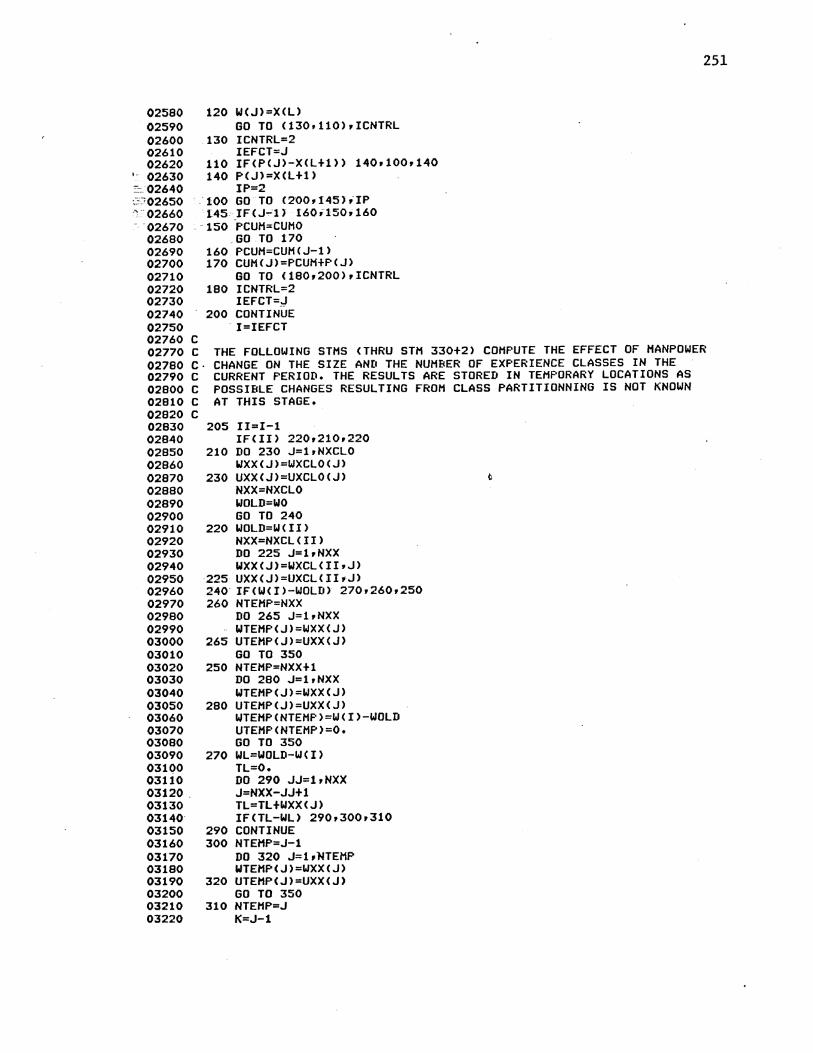
02580 02590

120 WCJ>=X<L>

02600 .130 02610 02620

I- 02630 110 140

GO TO C130rllO>riCNTRL ICNTRL=2 IEFCT=J IFCPCJ>-X<L+l>> 140r100r140 PC J>=XCL+l > IP=2 :::-:-.. 02640

;~<'02650 ·o2660 ·o267o 02680 02690 02700 02710 02720 02730

100 GO TO C200r145hiP 145 IFCJ~t> 160i150r160

. - 150 -PCUM,.CUMO

160 170

180

02740 200 02750

_GO TO 170 PCUH=CUMCJ-1> CUMCJ>=PCUH+PCJ) GO TO C180r200>riCNTRL ICNTRL=2 IEFCT=.J CONTINUE I=IEFCT

251

02760 c 02770 c 02780 c. 02790 c 02800 c 02810 c 02820 c 02830 02840 02850 02860 02870 02880

THE FOLLOWING STMS CTHRU STM 330+2> COMPUTE THE EFFECT OF MANPOWER CHANGE ON THE SIZE AND THE NUMBER OF EXPERIENCE CLASSES IN THE CURRENT PERIOD. THE RESULTS ARE STORED IN TEMPORARY LOCATIONS AS POSSIBLE CHANGES RESULTING FROM CLASS PARTITIONNING IS NOT KNOWN AT THIS STAGE.

02890 02900 02910 02920 02930 02940 02950 02960 02970 02980 02990 03000 03010

205 II=I-1 IFCII> 220r210r220

210 DO 230 J=lrNXCLO WXXCJ>=WXCLO<J>

230 UXX<J>=UXCLO<J> NXX=NXCLO WOLD=WO GO TO 240

220 WOLD=WCII> NXX=NXCLCII> DO 225 J=1rNXX WXXCJ)=WXCLCIIrJ>

225 UXXCJ>=UXCLCII,J> 240 IF<W<I>-WOLD> 270r260r250 260 NTEMP=NXX

DO 265 J=1rNXX WTEMP<J>=WXXCJ)

265 UTEMP<J>=UXXCJ> GO TO 350 NTEMP=NXX+1 03020 250

03030 DO 280 J=lrNXX WTEMP<J>=WXXCJ) UTEMP<J>=UXXCJ) WTEMP<NTEMP>=W<I>-WOLD UTEMP<NTEMP>=O.

03040 03050 280 03060 03070 03080 03090 270 03100 03110 03120. 03130 03140 03150 290 03160 300 03170 03180 03190 320 03200 03210 310 03220

GO TO 350 WL=WOLD-WCI) TL=O. DO 290 JJ=1rNXX J=NXX-JJ+1 TL=TL+WXXCJ) IFCTL-WL) 290r300r310 CONTINUE NTEMP=J-1 DO 320 J=lrNTEMP WTEMPCJ>=WXX<J> UTEMP<J>=UXXCJ) GO TO 350 NTEHP=J K=J-1

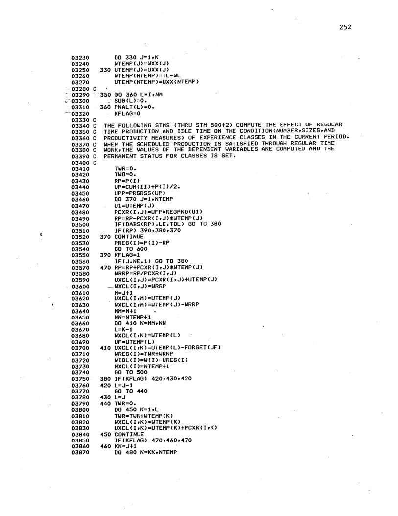
03230 03240 03250 03260 03270

c

330

DO 330 .J=1rl< WTEHP(.J)=WXX<.J> UTEHP<.J>=UXX<.J> WTEHPCNTEHP>=TL-WL UTEHP<NTEHP>=UXXCNTEMP>

252

-03280 ' 03290 '..'03300

- ·350 DO 360 ~·IrNH SUB<U=O.

. 03310 --o3320

03330 c 03340 c 03350 c 03360 c 03370 c 03380 c 03390 c 03400 c 03410 03420 03430 03440 03450 03460 03470 03480 03490 03500 03510 03520 03530 03540 03550 03560 03570 03580 03590 03600 03610 03620 03630 03640 03650 03660 03670 03680 03690 03700 03710 03720 03730 03740 03750 03760 03770 03780 03790 03800 03810 03820 03830 03840 03850 03860 03870

360 PNAL T<U=O. I<FLAG=O

THE FOLLOWING STHS CTHRU STH 500+2> COMPUTE THE EFFECT OF REGULAR TIME PRODUCTION AND IDLE TIME ON THE CONDITIONCNUMBERrSIZESrAND PRODUCTIVITY MEASURES) OF EXPERIENCE CLASSES IN .THE CURRENT PERIOD. WHEN THE SCHEDULED PRODUCTION IS SATISFIED THROUGH REGULAR TIME WORKrTHE VALUES OF THE DEPENDENT VARIABLES ARE COMPUTED AND THE PERMANENT STATUS FOR CLASSES IS SET.

TWR=O. TWO=O. RP=P< I> UP=CUH<II>+P<I>/2. UPP=PRGRSSCUP> DO 370 .J=1rNTEHP Ul=UTEHPC.J) PCXRCirJ>=UPP*REGPROCU1) RP=RP-PCXRCirJ>*WTEMPCJ) IF<DABS<RP>.LE.TOL> GO TO 380 IF<RP> 390r380r370

370 CONTINUE PREGCI>=PCI>-RP GO TO 600

390 I<FLAG=1 IFCJ.NE.1> GO TO 380

470 RP=RP+PCXRCirJ>*WTEMP<J> WRRP=RP/PCXRCirJ> UXCLCirJ>=PCXRClrJ)+UTEMPCJ>

- WXCL GI , J > =WRRP M=J+1 UXCLCirM>=UTEHP<J> WXCLCirH>=WTEMP<J>-WRRP HM=H+1 NN=NTEHP+l DO 410 I<=MMrNN L=K-1 WXCLCirK>=WTEHP<L> UF=UTEHP<L>

410 UXCLCirK>=UTEHPCL>-FORGETCUF> WREGCI)=TWR+WRRP WIDL<I>=W<I>-WREG<I> NXCL<I>=NTEMP+l GO TO 500

380 IFCI<FLAG> 420r430r420 420 L=.J-1

GO TO 440 430 L=.J 440 TWR=O.

DO 450 K=lrl TWR=TWR+WTEMP<K> WXCLCirK>=WTEMP<K> UXCLCirK>=UTEMP<K>+PCXRCirl<)

450 CONTINUE IF<KFLAG> 470r460r470

460 I<I<=J+l DO 480 I<=KI<rNTEHP

03880 03890 03900 03910 03920

-03930 e;-~03940

:=03950 :03960

- 03970 03980 c 03990 c 04000 c 04010 c 04020 c 04030 c 04040 04050 04060 04070 04080 04090 04100 04110 04120 04130 04140 04150 04160 04170 04180 04190 04200 04210 04220 04230 04240 04250 04260 04270 04280 04290 04300 04310 04320 04330 04340 04350 04360 04370 04380 04390 04400 04410 04420 04430 04440 04450 04460 04470 04480 04490 04500

. 04510 04520

UF=UTEMP <10 UXCLCirK)=UTEMPCK)-FORGETCUF)

480 WXCLCirK>=WTEMP<K> NXCL<I>=NTEMP WIDL<I>=WCI>-TWR

_ WREG<I->=TWR 500~PREG<I>=PCI)

=-u:-ovR< n=o. cWOVR<I>=O. -·Go_ TO_ 950

253

THE FOLLOWING STMS CTHRU STM 920+6> COMPUTE THE EFFECT OE OVERTIME PRODUCTION ON THE CONDITIONS OF EXPERIENCE CCASSES. THE VALUES OF THE DEPENDENT VARIABLES ARE COMPUTED AND THE PERMANENT CLASS STATUS IS SET FOR CLASSES IN THE CURRENT PERIOD.

600 DO 570 J=1rNTEMP U1-=UTEMPC J>+PCXR C I rJ> /2 PCXOCirJ>=UPP*OVRPROCU1> RP=RP-PCXOCirJ>*WTEMP<J> IFCDABSCRP>.LE.TOL> GO TO 580 IFCRP> 590r580r570

570 CONTINUE GO TO 900

590 KFLAG=1 IFCJ.NE.1>GO TO 580

670 RP=RP+PCXOCirJ>*WTEMPCJ) WROP=RP/PCXOCirJ> UXCLCirJ)=UTEMPCJ>+PCXOCirJ>+PCXRCirJ) WXCLCirJ>=WROP M=J+1 UXCLCirM>=UTEMPCJ>+PCXRCirJ) WXCLCirH>=WTEMPCJ>-WROP HH=M+l NN=NTEMP+l DO 610 K=MHrNN L=K-1 WXCLCirK>=WTEHP<L>

610 UXCL(IrK)=UTEMP<L>+PCXR(I;L) WOVR<I>=TWO+WROP NXCL<I>=NTEMP+1 GO TO 700

580IFCKFLAG> 620r630r620 620 L:::i:J-1

GO TO 640 630 L=J 640 TWO=O.

DO 650 K=1rL TWO=TWO+WTEMP<K> UXCLCirK>=UTEMPCK>+PCXR<IrK>+PCXOCirK>

650 WXCLCirK>=WTEMP<K> IF<KFLAG> 670r660r670

660 KK=J+l DO 680 K=KKrNTEMP UXCL<I•K>=UTEMP<K>+PCXRCirK)

680 WXCLCirK>=WTEHP<K> NX,k.LCI>=NTEMP WOVRCI>=TWO

700 POVRCI)=P<I>-PREG<I> WREGCI>=W<I> WIDLCI >=O. GO TO 950

900 NXCLCI)=NTEMP DO 920 J=1rNTEHP UXCLCirJ)=UTEHP<J>+PCXRCirJ>+PCXOCirJ)

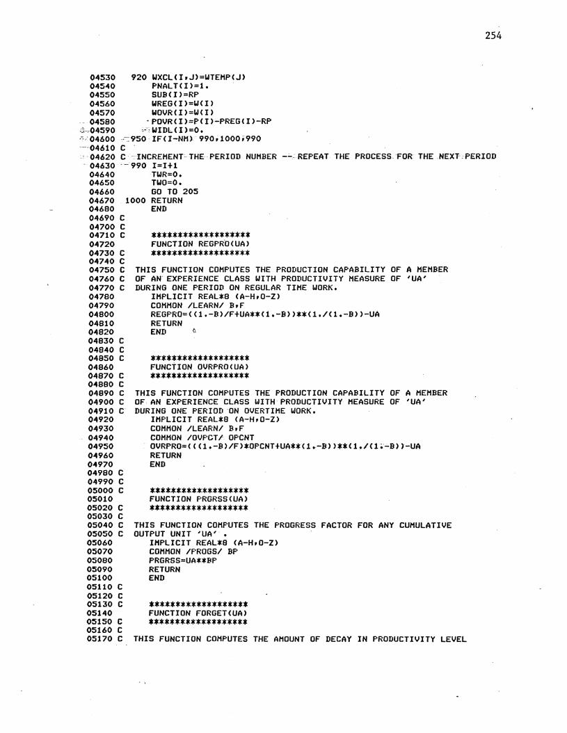
04530 920 WXCL(I,J>=WTEMPCJ> 04540 PNALTCI)=1. 04550 SUBCI>=RP 04560 WREGCI>=WCI> 04570 WOVR<I>=W<I>

- 04580 · POVRC I >=PC I >-PREG< I >-RP ~04590 "'"'WIDLCI>=O • . -::"·04600 -c-::950 IFH-NH> 990r1000i990 -~- 04610 c

254

04620 C INCREMENT THE PERIOD NUMBER REPEAT THE PROCESS.'FOR THE.NEXT PERIOD · 04630 - 990 I=I+l

04640 TWR=O. 04650 TWO=O. 04660 GO TO 205 04670 . 1000 RETURN 04680 END 04690 c 04700 c 04710 c 04720 04730 c 04740 c 04750 c 04760 c 04770 c 04780 04790 04800 04810 04820 04830 c 04840 c 04850 c 04860 04870 c 04880 c 04890 c 04900 c 04910 c 04920 04930 04940 04950 04960 04970 04980 c 04990 c 05000 c 05010 05020 c 05030 c 05040 c 05050 c 05060 05070 05080 05090 05100 05110 c 05120 c 05130 c 05140 05150 c 05160 c 05170 c

******************* FUNCTION REGPR.OCUA> *******************

THIS FUNCTION COMPUTES THE PRODUCTION CAPABILITY OF A MEMBER OF AN EXPERIENCE CLASS WITH PRODUCTIVITY MEASURE OF 'UA' DURING ONE PERIOD ON REGULAR TIME WORK.

IMPLICIT REAL*8 CA-H,O-Z> COMMON /LEARN/ B•F REGPRO=CC1.-B>IF+UA**Cl.-B>>**<1./C1.-B>>-UA RETURN END

******************* FUNCTION OVRPROCUA> *******************

THIS FUNCTION COMPUTES THE PRODUCTION CAPABILITY OF A MEMBER OF AN EXPERIENCE CLASS WITH PRODUCTIVITY MEASURE OF 'UA' DURING ONE PERIOD ON OVERTIME WORK.

IMPLICIT REAL*8 <A-HrO-Z) COMMON /LEARN/ BrF COMMON /OVPCT/ OPCNT OVRPR0=<<<1.-B>IF>*OPCNT+UA**<1~-B>>**<l./(1~-B>J-UA RETURN END

******************* FUNCTION PRGRSSCUA> *******************

THIS FUNCTION COMPUTES THE PROGRESS FACTOR FOR ANY CUMULATIVE OUTPUT UNIT 'UA' •

IMPLICIT REAL*8 CA-H•O-Z> COMMON /PROGS/ BP PRGRSS==UA**BP RETURN END

******************* FUNCTION FORGETCUA> *******************

THIS FUNCTION COMPUTES THE AMOUNT OF DECAY IN PRODUCTIVITY LEVEL

05180 c 05190 c 05200 05210 05220

_-_05230 ~.::05240

OVER ONE PERIOD FOR A MEMBER OF A CLASS WITH PRODUCTIVITY MEASURE OF 'UA' AT THE BEGINNING OF THE PERIOD.

IMPLICIT REAL*B <A-HrO-Z> COMMON /FORGT/ BFrF1 FORGET=<<1.-BF>IF1tUA**<1.-BF>>**<1~/(1.-BF>>-UA RETURN

_ END

255

""".05250 c _c::~05260.C

;_ 05270 c ~ _05280 c

05290 c 05300 c 05310 c 05320

-05330 c

c c

~~***************************** - * . * * PATTERN-SEARCH SUBROUTINE * * _. * *****************************

SUBROUTINE PATS

THIS ROUTINE IS BASED LARGEL~ ON PRIO~ WORK BY TAUBERT WHOr IN TURNr RELIED HEAVILY ON A PRIOR SEARCH ROUTINE SOURCE CODE BY WEISMAN-WOOD-RIVLINrWHICH WAS ITSELF AN ADAPTATION OF THE ORIGINAL HOOKE-JEEVES PATTERN SEARCH.THE ROUTINE IS OBTAINED FROM A PART OF THE RESEARCH CONDUCTED BY TOM SIKES CUCLA>rRELATIVE TO THE SDR APPLICATION IN THE AGGREGATE PLANNING PROBLEM. THE CODE IS DIVIDED INTO 18 SUBSETS CALLED 'BOXES' rWITH ENTRANCES AND EXITS FOR EACH BOX EXHAUSTIVELY IDENTIFIED •. THIS FORMS A COMPLETE BASIS FOR A FLOW CHARTr IF THE NEED SHOULD ARISE,

IMPLICIT REAL*8 <A-HrO-Z) DIMENSION DC20>rGC20) COMMON /SHARE/ XC40>rN•NMrSN COMMON /SRCHP/ XMAXC20>rXMINC20)rLIHrKPRESSrNO COMMON /VALUE/ NEVAL

05340 .c 05350 c 05360 c 05370 ·c 05380 c 05390 c 05400 c 05410 c 05420 c 05430 c 05440 c 05450 c 05460 c 05470 c 05480 05490 05500 05510 05520 05530 05540 05550 C <BOX 1> PURPOSE: INIT-IALIZE DATA. ENTRANCES: FROM START OF THE

c- SUBROUTINE AND FROM.:cBOX-18"VIA-STM·100t EXITS: T0190 IN-BOX.S. c

.. 05560 05570 05580 05590 05600 05610 05620

. 05630 05640 05650 05660 05670 05680 05690 05700 05710 05720 05730 05740 05750 05760 05770 05780 05790 05800 05810 05820

100 TOL=1.E-S BET=.l DEL=o1 LT=O LSN=O NPF=O ITR=l ALP=2. GR=2.2 LA=l LT2=0 LT3=0 LT4=0 LT5=0 LT6=0 LT7=0 ID1=0

.ID2=0 ID3=0 ID4=0 KOUNT=O V=O. OLIIV=O. NEVOLD=O DO lSO I=1rN

256

05830 0!5840 c 0!5850 c 0!5860 c

'05870 _: 0!5880 ~-0!5890 ~·· 0!5900 --·0!5910 .• 05920 . -05930

05940 0!5950 05960 05970 05980 05990 06000 06010 06020 06030 06040 c 06050 c 06060 c 06070 c 06080 c 06090 c 06100 c 06110 c

Q( I >=X<I > NOTE FROH THE NEXT STATEMENT THAT THE INITIAL VALUE OF DCK) DEPENDS ON HOW FAR APART THE UPPER AND LOWER BOUNDRIES ARE.

180 DCI>=DEL*CXHAXCI>-XHINCI>> CALL F:CT1

:.:. :.SNOLD=-~'1 '" Ol:[ISN=SN .. SC=SN · ::::sp .. sN

H1=1 H2=1 K=1 KK=1 L4=1 IFCKPRESS.NE.O> GO TO 190 WRITECNOr999> DEL

999 FORHATC'O~j20Xr'PATTERN SEARCH DEL='rF6.2> WRITECNOr991)NEVALrKOUNTrLT2rLT3rLT4rLT5rLT6rLT7rKrKKrH1rH2rNPFr

1LArL4riD1riD2riD3riD4rSNrVrGRrDC1>rDC2JrDC3) -GO TO 190

<BOX 18> PURPOSE: CALL OBJECTIVE FUNCTION. ENTRANCES: FROM BOXES 17r 7r AND 14. EXITS: TO STHS 100 AND 500r TO 282 AND 285 IN BOX 2r TO 463 AND 466 IN BOX 11r AND TO 580 IN BOX 15r TO 510 IN BOX 13. COMMENT: 'LA' CONTROLS THE TRAFFIC THROUGH THIS BOXr SEE GLOSSARY FOR INTERPRETATION OF VALUES OF LA.

06120 ·270 CALL FCT1 06130 GO TO C100r282r463r580r285r466r510r500)rLA 06140 c 06150 c 06160 c 06170 c 06180 c 06190 c 06200 c 06210 c 06220 c 06230 06240 06250 06260 06270 c 06280 06290 c 06300 c 06310 c 06320 06330 c 06340 c 06350 c 06360 c 06370 c 06380 06390 06400 06410 06420 c 06430 c 06440 c 06450 c 06460 c 06470 c

<BOX 2> PURPOSE: EVALUATE FORWARD MOVES. ENTRANCES:FROH BOX 18 VIA STHS-282 ANI! 285 •. EXITS: TO 360 IN BOX 6 WHEN FORWARD HOVE FAILSr TO 300 IN BOX 3 WHEN FORWARD HOVE SUCCEEDS. COMMENT: THIS BOX IS REACHED WHEK LA=2 OR 5.

INCREMENT STATE COUNTER

282 LT2=LT2+1 GO TO 280

. 285 L TS=L T5+ 1 280 IFCSN-SP>290•360r360

TEST FOR SUCCESS OR FAILURE C290r OR 360) 290 GO TO C300r292)rL4

IF THE SEARCH IS IN AN EXPLORATORY MODE FOLLOWING AN ATTEMPTED PATTERN MOVErMULTIPLY THIS SUCCESSFUL FORWARD STEP SIZE BY ALP.

292 D<K>=D<K>*ALP

<BOX 3> PURPOSE: RESET SOME VARIABLES. ENTRANCES: FROM BOXES 2 AND 11rBOTH VIA 5TH 300. EXIT: TO 305 IN BOX 4.

300 SP=SN M2=1 M1=1 HPF=O

<BOX 4> PURPOSE: DECIDE WHETHER TO TEST FOR A NEW BASE POINT. ENTRANCES: FROM BOXES 3 AND 12 VIA STH 305. EXITS:TO 340 IN IN BOX 7 WHEN A BASE POINT TEST IS REQUIRED• TO 200 IN BOX 5 OTHERWISE. COMMENT: THIS BOX IS THE ONLY ENTRANCE TO THE BASE

257

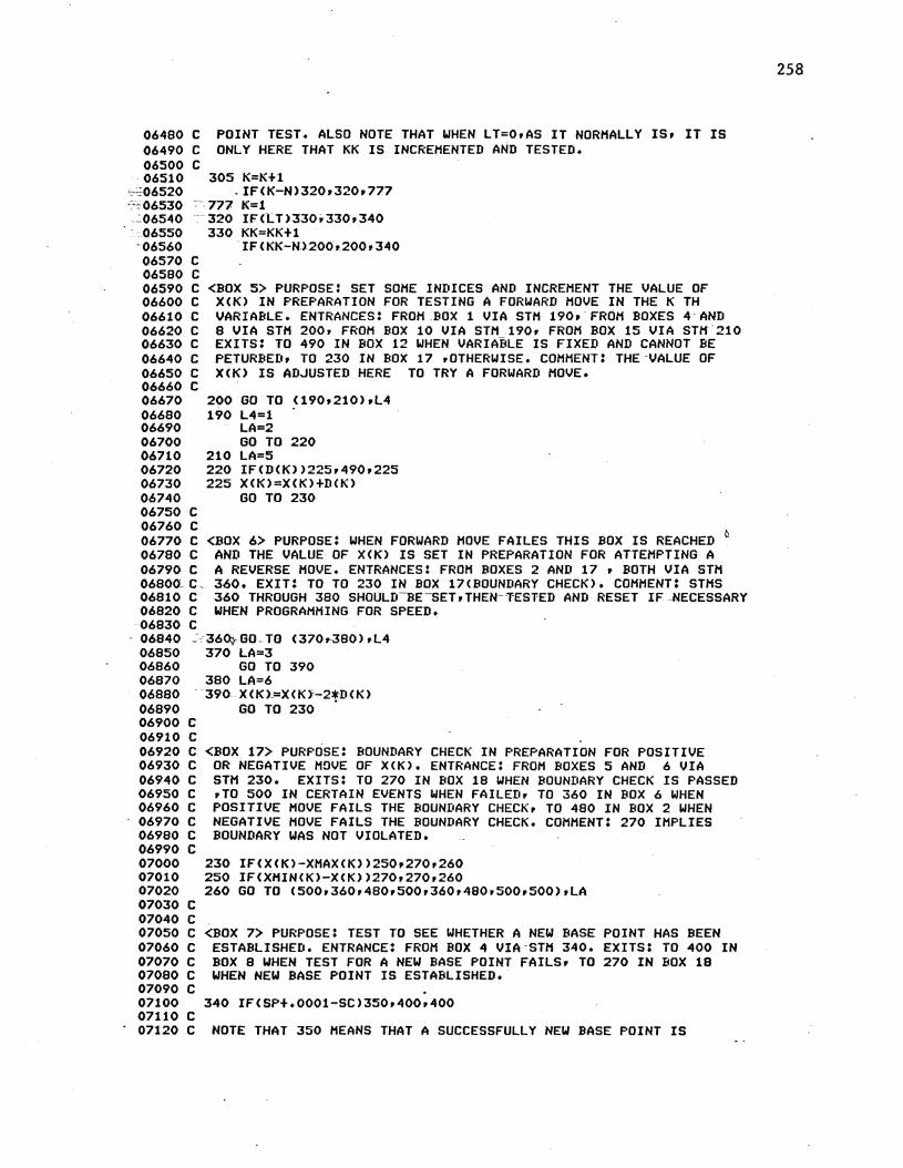
06480 06490 06500 06510

C POINT TEST. ALSO NOTE THAT WHEN LT=O•AS IT NORMALLY IS• IT IS C ONLY HERE THAT KK IS INCREMENTED AND TESTED. c

':';i:06520 ·Y06530 -~06540 •c06550

305 K=K+l -IF<K-N>320r320r777

~-777 l<=l -320 IF(LT)330r3309340 330 l<K=KK+l

~o6560

06570 c 06580 c 06590 c 06600 c 06610 c 06620 c 06630 c 06640 c 06650 c 06660 c 06670 06680 06690 06700 06710 06720 06730 06740 06750 c 06760 c 06770 c 06780 c 06790 c 06800- c' 06810 c 06820 c 06830 c

IF (I\K-N>200-,200r340

<BOX 5> PURPOSE: SET SOME INDICES AND INCREMENT THE VALUE OF X<K> IN PREPARATION FOR TESTING A FORWARD MOVE IN THE K TH VARIABLE. ENTRANCES: FROM_BQX 1 VIA STM 190r FROM BOXES 4 AND 8 VIA STM 200r FROM BOX 10 VIA STM 190r FROM BOX 15 VIA STK-210 EXITS: TO 490 IN BOX 12 WHEN VARIABLE IS FIXED AND CANNOT BE PETURBEBr TO 230 IN BOX 17 rOTHERWISE. COMMENT: THE-VALUE OF X<K> IS ADJUSTED HERE TO TRY A FORWARD MOVE.

200 GO TO C190r210>rL4 190 L4=1

LA=2 GO TO 220

210 LA=5 220 IF<D<K>>225•490•225 225 X<K>=XCK>+D<K>

GO TO 230

<BOX 6> PURPOSE: WHEN FORWARD HOVE FAILES THIS BOX IS REACHED 0

AND THE VALUE OF X<K> IS SET IN PREPARATION FOR ATTEMPTING A A REVERSE MOVE. ENTRANCES: FROM BOXES 2 AND 17 , BOTH VIA STM 360. EXIT: TO TO 230 IN BOX 17<BOUNDARY CHECK>. COMMENT: STMS 360 THROUGH 380 SHOULD-BE--SET, THE:N- T-ESTED AND RESET IF- --NECESSARY WHEN PROGRAMMING FOR SPEED.

- 06840 ~,, 36~,-GO-TO (370r-380-> •L4 06850 370 LA=3 06860 GO TO 390 06870 380 LA=6 06880 390 XCK>.=X<Kl-2~D<K> 06890 GO TO 230 06900 c 06910 c 06920 c 06930 c 06940 c 06950 c 06960 c 06970 c 06980 c 06990 c 07000 07010 07020 07030 c 07040 c 07050 c 07060 c 07070 c 07080 c 07090 c

<BOX 17> PURPOSE: BOUNDARY CHECK IN PREPARATION FOR POSITIVE OR NEGATIVE MOVE OF X<K>. ENTRANCE: FROM BOXES 5 AND 6 VIA STH 230. EXITS: TO 270 IN BOX 18 WHEN BOUNDARY CHECK IS PASSED rTO 500 IN CERTAIN EVENTS WHEN FAILEDr TO 360 IN BOX 6 WHEN POSITIVE MOVE FAILS THE BOUNI•ARY CHECKr TO 480 IN BOX 2 WHEN NEGATIVE MOVE FAILS THE BOUNDARY CHECK. COMMENT: 270 IMPLIES BOUNDARY WAS NOT VIOLATED.

230 IF<X<K>-XMAX<K>>2S0r270•260 250 IF<XHIN<K>-X<K>>270,270r260 260 GO TO (500r360,480r500,360r480r500r500)rLA

<BOX 7> PURPOSE: TEST TO SEE WHETHER A NEW BASE POINT HAS BEEN ESTABLISHED. ENTRANCE: FROM BOX 4 VIA STM 340. EXITS: TO 400 IN BOX 8 WHEN TEST FOR A NEW BASE POINT FAILSr TO 270 IN BOX 18 WHEN NEW BASE POINT IS ESTABLISHED.

07100 340 IFCSP+.0001-SC>350r400r400 07110 c 07120 c NOTE THAT 350 MEANS THAT A SUCCESSFULLY NEW BASE POINT IS

258

07130 c 07140 c 07150 c

IDENTIFIED.IF L4=1r THE FIRST PATTERN MOVE IN THIS SERIES IS TO BE ATTEMPTED.

07160 350 GO TO <352r353>rL4 07170 352 LA=7 07180 Hl=l

: -07190 :__ GO- ·nr :210 '' 07200 ,:-353 IF<NPF-5>-352,400r400 --·onto- c --07220 c

-07230 C <BOX B> PURPOSE: HAVING f'AILED .TO £STABLISH A NEW BASE POINTr- THIS 07240 C BOX IS REACHED TO DECIDE WHERE TO GO NEXT~ ENTRANCE:-FROM BOX 7 07250 C VIA STH 400. EXITS: TO 200 IN BOX 5 WHEN KK.LE.Nr AFTER BASE POINT 07260 C TEST; WHEN FAILURE OCCURED AT THE CONCLUSION OF ADJUSTMENTS 07270 C FOLLOWING AN ATTEMPTED PATTERN HOVErAND TO 440 IN BOX 10 WHEN IN 07280 C THE PROCESS OF SEARCHING FOR A PATTERN AND THE VALUE OF H1 IS LESS 07290 C -THAN Nfl-TO 500 IN BOX 16 WHEN NO NEW PATTERN IS FOUND AND-SEARCH 07300 C IS TO BE ESTABLISHED. 07310. c 07320 07330 07340 07350 07360 07370. 07380 c 07390 c 07400 c 07410 c 07420 c 07430 c 07440 07450 07460 07470 07480 c 07490 c

400 IFCLT)404r404r778 778 KK=KKfl 404 IF<KK-N>200r200r779 779 GO TO <429r410>rL4 429 L4=2

IF<Hl-N>440r440r500

<BOX 9> PURPOSE:RESTORE THE VALUES OF XCI> AFTER UNSUCCESSFUL ATTEMPT TO ESTABLISH NEW BASE POINT. ENTRANCE: FROH BOX 8 VIA STH 410. EXIT4 TO 440 IN BOX 10.

410 SP=SC DO 420 I=1rN

420 X< I >=IHI> NPF=O

07500 C <BOX 10> PURPOSEl REST SOME COUNTERS CSEE GLOSSARY FOR-DEFINITIONS> - 07510 C·-c-ENTRANCE: FROH BOX S--ANn 9r~ BOTH VIA STH 440. EXIT: T0-190 INc BOX S.

07520 c 07530 07540

~-07550

07560 07570 c 07580 c 07590 c 07600 c 07610 c 07620 c 07630 c 07640 C. 07650 c 07660 07670 07680 07690

- 07700 c

440 H2=1 Hl=l t<K=l

-Go TO 190

<BOX 11> PURPOSE: EVALUATE A REVERSE MOVE (CORRESPONDING TO BOX 2'S FORWARD MOVE EVALUATION>.ENTRANCE: FROM BOX 18 VIA STMS 463r466. EXITS: TO 480 IN BOX 12 WHEN WHEN REVERSE MOVE FAILS, TO 300 IN BOX 3 WHEN REVERSE MOVE SUCCEEDS. COMMENT: NOTE THAT NAS USUAL THE COUNTERS LT3 AND LT6 ARE SETr DEPENDING WHETHER THIS BOX IS REACHED WITH LA=3 OR 6.

463 LTJ=LJ+l GO TO 460

466 LT6=LT6f1 460 IF<SN-SP>470r480r480

07710 C SUCCESS! THEREFORE IN THE FUTURE A FORWARD HOVE WILL BE WHAT HAS 07720 C HERETOFORE BEEN A BACKWARD HOVE - HENCEr ST" 470 07730 c 07740 470 DCK>=-DCK> 07750 GO TO 300 07760 c 07770 c

259

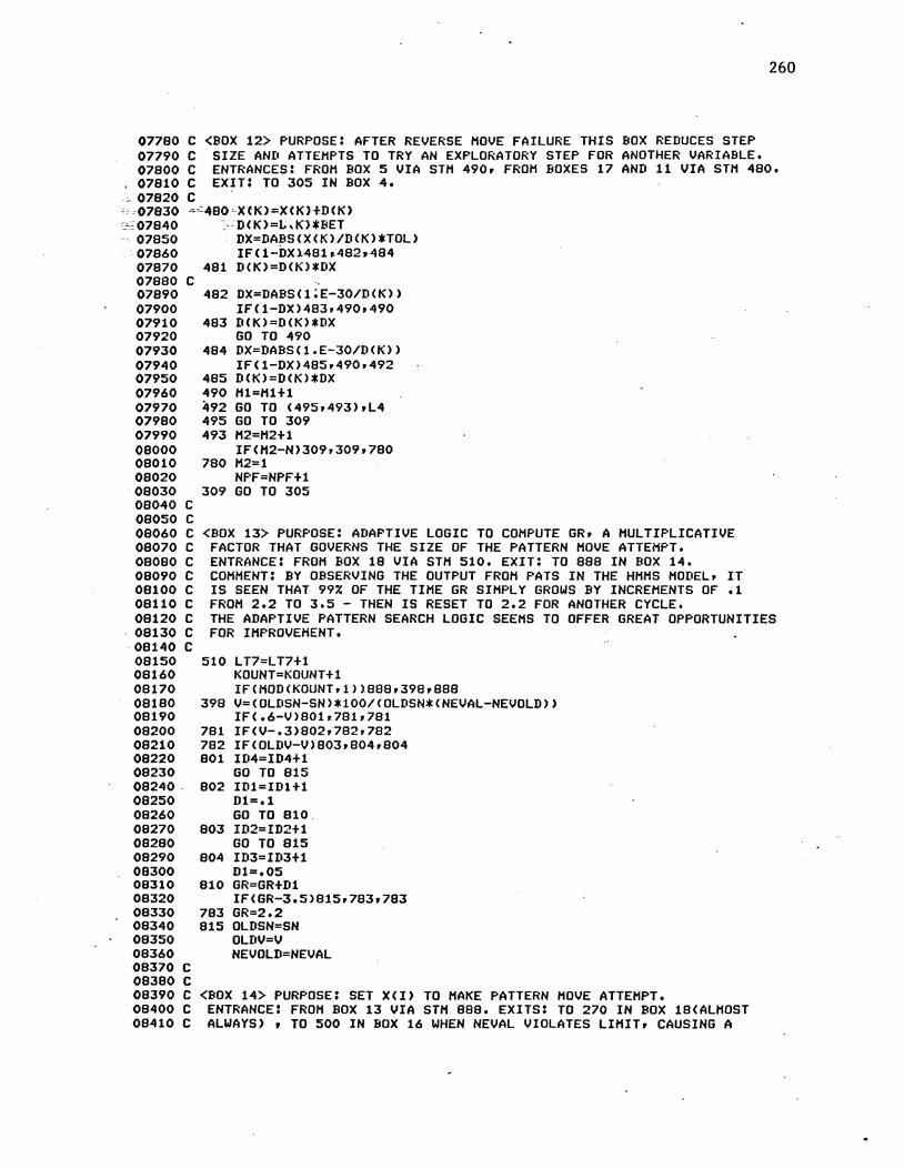
260

07780 c 07790 c 07800 c 07810 c

<BOX 12> PURPOSE: AFTER REVERSE MOVE FAILURE THIS SIZE AND ATTEMPTS TO TRY AN EXPLORATORY STEP FOR ENTRANCES: FROM BOX 5 VIA STM 490r FROM BOXES 17 EXIT: TO 305 IN BOX 4.

BOX REDUCES STEP ANOTHER VARIABLE. AND 11 VIA STH 480.

0 07820 c ·~07830 ~~480cXCK>=XCK}fDCK>

:~~07840 "-- D<IO=L.IO*BET 07850 DX=DABSCXCK>/DCK>*TOL> 07860 IF <1-DX >.481 ~482 ,494 07970 481 D<K>=DCK>*DX 07880 c 07890 482 07900 07910 483 07920 07930 484 07940 07950 07960 07970 07980 07990 08000 08010 08020

485 490 492 495 493

780

DX=DABS(1;E-30/DCK>> IF<1-DX>483r490r490 D<K>=DCK>*DX GO TO 490 DX=DABSC1.E-30/DCK>> IF<1-DX>485r490r492 DCK>=D<K>*DX H1=H1t1 GO TO C495r493)rL4 GO TO 309 H2=H2+1 IFCH2-N>309r309r780 M2=1 NPF=NPF+l GO TO 305 08030 309

08040 c 08050 c 08060 c 08070 c 08080 c 08090 c 08100 c 08110 c 08120 c

<BOX 13> PURPOSE: ADAPTIVE LOGIC TO COMPUTE GRr A MULTIPLICATIVE FACTOR THAT GOVERNS THE SIZE OF THE PATTERN HOVE ATTEMPT. ENTRANCE: FROM BOX 18 VIA STM 510. EXIT: TO 888 IN BOX 14. COMMENT: BY OBSERVING THE OUTPUT FROM PATS IN THE HHHS HODELr IT IS SEEN THAT 99% OF THE TIME GR SIMPLY GROWS BY INCREMENTS OF .1 FROM 2.2 TO 3.5 - THEN IS RESET TO 2.2 FOR ANOTHER CYCLE.

.. 08130 c 08140C 08150 08160 08170

THE ADAPTIVE PATTERN SEARCH LOGIC SEEMS TO OFFER GREAT OPPORTUNITIES FOR IMPROVEMENT.

510 LT7=LT7+1

08180 398 08190

KOUNT=KOUNT+1 IFCMODCKOUNTr1))888r398r888 V=<OLDSN-SN>*100/COLDSN*CNEVAL-NEVOLD>> IFC.6-V>801r781r781

08200 08210 08220 08230 08240. 08250 08260 08270 08280 08290 08300 08310 08320 08330 08340 08350 08360 08370 c 08380 c 08390 c 08400 c 08410 c

781 782 801

IF<V-.3)802i782r782 IFCOLDV-V)803r804r804 ID4=ID4+1 GO TO 815

802 ID1=ID1+1 D1=.1 GO TO 810.

803 ID2=ID2+1 GO TO 815

804 ID3=ID3+1

810

783 815

D1=.05 GR=GRtD1 IF<GR-3.5>815r783r783 GR=2.2 OLDSN=SN OLDV=V NEVOLD=NEVAL

<BOX 14> PURPOSE: SET XCI> TO MAKE PATTERN HOVE ATTEMPT. ENTRANCE: FROM BOX 13 VIA STH 888. EXITS: TO 270 IN BOX 1BCALMOST ALWAYS> r TO 500 IN BOX 16 WHEN NEVAL VIOLATES LIHITr CAUSING A

08420 c 08430 c 08440 c 08450 c

. 08460 c " 0 '08470 i.,-"08480 ~'=.08490

08500 .. 08510

08520 08530 08540 08550 08560 08570 08~80

08590 08600 08610 08620 08630 08640 08650 08660 08670 08680 c 08690 c 08700 c 08710 c 08720 c 08730 c 08740 08750 08760 08770 08780 c

RETURN TO THE MAIN ROUTINE. COMMENT! NOTICE THAT A BOUNDARY CHECK IS CONTAINED IN THIS BOX AND IS SLIGHTLY DIFFERENT FROM THE ONE IN BOX 17 INSOFAR AS THE CONCEOUNCES OF FAILING THE CHECK ARE CONCERNED.

888 IFCHODCKOUNTtiTRt>7r8r7 0 B~IFCKPRESS.NE~O>~GO~TO 7

WRITECNOr991>NEUALrKOUNTrlT2,LT3rLT4.Ll5rLT6•LT7rKrKKrH1rH2rNPFr 1LA•L4riD1~ID2~ID3~ID4~SNrVrGRrD<1>rD<2>rD{3)

7 JFCLIH-NEVAL}500,~84t784 784 KK=1

IF<LSN>S30r530•785 785 SP=SN 530 SC=SP

LA=4 DQ-570 I=1 rN P=QCI> an>=X<I> X<I>=P+GR*CXCI)-P) IFCXCI>-XHAX<I>>550r570•786

786 X<I>=XHAX<l> GO TO 570

550 IFCXHINCI>-X<I>>S70r570r787 787 X <I >.;,XHINC I> 570 CONTINUE

GO TO 270

<BOX 15> PURPOSE: SET CERTAIN COUNTERS PRIOR TO ADJUSTMENTS OF THE PATTERN HOVE ATTEMPT. ENTRANCE: ~OM BOX 18 VIA STH 580. EXIT! TO 210 IN BOX 5 ALWAYS.

sao LT4=LT4+1 L4=2 SP=SN GO TO 210

Q

<BOX 16> SEARCH. VIA STH

500 LA=B

PUPOSE! PRINT OUT FINAL PARAMETER VALUES AND TERMINATE THE ENTRANCE! FROM BOXES 17 AND 18 r FROM BOXES 8 AND 14 r ALL 500. EXIT~ RETURN TO THE MAIN ROUTINE.

990 WRITECNOr1111)

. 08790 c 08800 c 08810 c 0.8820 c 08830 c 08840 08850

.08860· 08870 08880

1111 FORMAT< 1HO) WRITECN0.991)NEVAL,KOUNT,LT2•LT3rLT4rLT5rLT6,LT7rKrKKrH1•H2rNPFr

1LA•L4•ID1,ID2tiD3riD4rSNrVrGR,DC1>•D<2),DC3> 08890 08900 08910

991 FORHATC1H •l5r4I4,1X,3I4r4I3t3I2•1Xr4I3,F14.4rFB.S,F5.2•3F9.6> RETURN END

END OF DATA

261

VITA

Behrokh Khoshnevis

Candidate for the Degree of

Doctor of Philosophy

Thesis: AGGREGATE PRODUCTION PLANNING MODELS INCORPORATING DYNAMIC PRODUCTIVITY

Major Field: Industrial Engineering and Management

Biographical:

Personal Data: Born in Sari, Iran, December 31, 1950, the son of Mr. and Mrs. Islam Khoshnevis.

Education: Graduated from Azar High School, Tehran, Iran, in June, 1969; received Bachelor of Science degree in Industrial Engineering from Arya-Mehr University of Technology, Tehran, Iran, in January, 1974; received Master of Science degree in Industrial Engineering and Management from Oklahoma State University in December, 1975; completed requirements for the Doctor of Philosophy degree at Oklahoma State University in December, 1979.

Professional Experience: Instructor of Physics and Technical Graphics in Tehran public high schools, 1970-1973; Assembly Line Supervisor, Mercedes Benz Factory, Tehran, summer, 1972; Graduate Research and Teaching Assistant, Oklahoma State University, 1975-1979; Visiting Assistant Professor, teaching Operations Research, Dynamic Programming, Systems Simulation and Project Management, Oklahoma State University, 1979 to present.

Professional Organizations: American Institute of Industrial Engineers, Operations Research Society of America, The Institute of Management Sciences, Alpha Pi Mu.