
Data Assimilation under Geological Constraints
159
Data Assimilation under Geological Constraints Proefschrift ter verkrijging van de graad van doctor aan de technische Universiteit Delft, op gezag van de Rector Magnificus prof. ir. K.C.A.M. Luyben, voorzitter van het College voor Promoties, in het openbaar te verdedigen op donderdag 18 december 2014 om 10.00 uur door Bogdan Marius SEBACHER Master of Science in Mathematics geboren te Bucuresti, Romania.
-
Upload
khangminh22 -
Category
Documents
-
view
4 -
download
0
Transcript of Data Assimilation under Geological Constraints
Data Assimilation under GeologicalConstraints
Proefschrift
ter verkrijging van de graad van doctoraan de technische Universiteit Delft,
op gezag van de Rector Magnificus prof. ir. K.C.A.M. Luyben,voorzitter van het College voor Promoties,
in het openbaar te verdedigen opdonderdag 18 december 2014 om 10.00 uur
door
Bogdan Marius SEBACHER
Master of Science in Mathematicsgeboren te Bucuresti, Romania.

Dit proefschrift is goedgekeurd door de promotor:Prof. dr. ir. A. W. Heemink
Samenstelling promotiecomissie:
Rector Magnificus voorzitterProf. dr. ir. A. W. Heemink, Technische Universiteit Delft, promotorProf. dr. ir. J. D. Jansen, Technische Universiteit DelftProf. dr. S. M. Luthi, Technische Universiteit DelftProf. dr. F .H. J. Redig, Technische Universiteit DelftProf. dr. R. Trandafir, Universitatea Tehnica de Constructii Bucuresti, RomaniaAssociate Prof. dr. I. Hoteit, KAUST, Saudi ArabiaDr. R. G. Hanea, Statoil, NorwayProf. dr. ir. C. Vuik, Technische Universiteit Delft, reservelid
Copyright ©2014 by Bogdan Marius SebacherAll rights reserved. No part of the material protected by this copyright notice may bereproduced or utilized in any form or by any means, electronic or mechanical, includingphotocopying, recording or by any information storage and retrieval system, without theprior permission of the author.
ISBN: 978-94-6186-405-5Typeset by the author with the LATEXDocumentation System.On the cover: drawing by Maria Sebacher.Printed in The Netherlands by Gildeprint, Enschede.

To my family

Contents
Contents i
Acknowledgements iv
1 Introduction 11.1 Petroleum Systems . . . . . . . . . . . . . . . . . . . . . . . . . . . . 11.2 Data assimilation in reservoir engineering . . . . . . . . . . . . . . . . 31.3 Geologically consistent data assimilation . . . . . . . . . . . . . . . . . 51.4 Research objectives . . . . . . . . . . . . . . . . . . . . . . . . . . . . 71.5 Thesis outline . . . . . . . . . . . . . . . . . . . . . . . . . . . . . . . 8
2 Geological Simulation Models 92.1 Truncated plurigaussian simulation (TPS) . . . . . . . . . . . . . . . . 9
2.1.1 The Gaussian random fields . . . . . . . . . . . . . . . . . . . 92.1.2 The truncated plurigaussian simulation model (TPS) . . . . . . 15
2.2 Multiple-point geostatistical simulation (MPS) . . . . . . . . . . . . . . 202.2.1 The (discrete) training image . . . . . . . . . . . . . . . . . . . 202.2.2 The simulation models . . . . . . . . . . . . . . . . . . . . . . 22
3 Ensemble methods 243.1 Data assimilation basics . . . . . . . . . . . . . . . . . . . . . . . . . . 243.2 Ensemble methods for nonlinear filtering problems . . . . . . . . . . . 27
3.2.1 The nonlinear filtering problem . . . . . . . . . . . . . . . . . 293.2.2 The ensemble Kalman filter . . . . . . . . . . . . . . . . . . . 303.2.3 The EnKF methodology for state and parameter estimation . . . 313.2.4 The adaptive Gaussian mixture (AGM) and its iterative variant
(IAGM) . . . . . . . . . . . . . . . . . . . . . . . . . . . . . . 33i
ii CONTENTS
4 A probabilistic parametrization for geological uncertainty estimation us-ing the Ensemble Kalman Filter (EnKF) 364.1 Introduction . . . . . . . . . . . . . . . . . . . . . . . . . . . . . . . . 364.2 The Method Description . . . . . . . . . . . . . . . . . . . . . . . . . 40
4.2.1 The "probabilities fields" . . . . . . . . . . . . . . . . . . . . . 404.2.2 Geological simulation model (Assigning the facies on the grid) . 424.2.3 Truncation parameters . . . . . . . . . . . . . . . . . . . . . . 44
4.3 Ensemble Kalman filter implementation for facies update . . . . . . . . 444.3.1 State vector . . . . . . . . . . . . . . . . . . . . . . . . . . . . 444.3.2 Measurements . . . . . . . . . . . . . . . . . . . . . . . . . . 454.3.3 The EnKF implementation . . . . . . . . . . . . . . . . . . . . 454.3.4 Indicators for the quality of the estimations . . . . . . . . . . . 49
4.4 Reservoir description . . . . . . . . . . . . . . . . . . . . . . . . . . . 504.5 Cases presented . . . . . . . . . . . . . . . . . . . . . . . . . . . . . . 51
4.5.1 Case 1: Simulation model generated using isotropic random fields 524.5.2 Case 2: Simulation model generated using anisotropic random
fields . . . . . . . . . . . . . . . . . . . . . . . . . . . . . . . 584.5.3 Case 3: Uncertainty in the geostatistical properties of the Gaus-
sian fields . . . . . . . . . . . . . . . . . . . . . . . . . . . . 604.6 Appendix: The facies proportion impact . . . . . . . . . . . . . . . . . 61
5 An adaptive plurigaussian simulation (APS) model for geological uncer-tainty quantification using the EnKF 655.1 Introduction . . . . . . . . . . . . . . . . . . . . . . . . . . . . . . . . 655.2 The geological simulation model. . . . . . . . . . . . . . . . . . . . . . 69
5.2.1 The Motivation . . . . . . . . . . . . . . . . . . . . . . . . . . 695.2.2 The adaptive plurigaussian simulation model (APS) . . . . . . . 695.2.3 The impact of the facies simulation map . . . . . . . . . . . . . 74
5.3 Ensemble Kalman Filter (EnKF) implementation . . . . . . . . . . . . 755.3.1 The Work Flow . . . . . . . . . . . . . . . . . . . . . . . . . . 76
5.4 Case studies . . . . . . . . . . . . . . . . . . . . . . . . . . . . . . . . 795.4.1 The model with three facies types . . . . . . . . . . . . . . . . 795.4.2 The model with four facies types . . . . . . . . . . . . . . . . . 84
5.5 Appendix: The probability integral transform . . . . . . . . . . . . . . 89
6 Bridging multiple point geostatistics and truncated Gaussian fields forimproved estimation of channelized reservoirs with ensemble methods 916.1 Introduction . . . . . . . . . . . . . . . . . . . . . . . . . . . . . . . . 916.2 Parameterization and truncation in the Gaussian space . . . . . . . . . . 96
CONTENTS iii
6.3 Iterative Adaptive Gaussian Mixture Filter . . . . . . . . . . . . . . . . 996.3.1 The State Vector . . . . . . . . . . . . . . . . . . . . . . . . . 1016.3.2 The Resampling . . . . . . . . . . . . . . . . . . . . . . . . . 102
6.4 Applications . . . . . . . . . . . . . . . . . . . . . . . . . . . . . . . . 1036.4.1 Channelized reservoir with 2500 grid cells . . . . . . . . . . . 1056.4.2 Channelized reservoir with 10000 grid cells . . . . . . . . . . . 114
7 Realistic facies simulation with the APS model for a North Sea field case 1197.1 Introduction . . . . . . . . . . . . . . . . . . . . . . . . . . . . . . . . 1197.2 The geological setup . . . . . . . . . . . . . . . . . . . . . . . . . . . 1217.3 Integrated workflow . . . . . . . . . . . . . . . . . . . . . . . . . . . . 122
7.3.1 Fast modelling update (FMU) concept . . . . . . . . . . . . . . 1227.3.2 Reservoir model building workflow . . . . . . . . . . . . . . . 123
7.4 Set-up of the field case and results . . . . . . . . . . . . . . . . . . . . 123
8 Conclusions 1308.1 Conclusions . . . . . . . . . . . . . . . . . . . . . . . . . . . . . . . . 130
Bibliography 135
Summary 143
Samenvatting 146
About the Author 149

Acknowledgements
This thesis is the outcome of the joint effort of many people that contributed either byplaying an important role and taking active part in it or by generously sharing theirknowledge and sparkling ideas or by simply inspiring me during our conversations.
Firstly, I am at a loss for words to express my gratitude to my supervisor ArnoldHeemink for the help, guidance and support he offered me during my PhD research.Without his assistance and active participation in every step of the way, this thesis mayhave never been completed. Thank you very much for your encouragement and under-standing over these past four years.
Secondly, I am infinitely grateful to my "angel", Remus Hanea. He was close to meduring important moments, offering me opportunities, finding resources and above allinvesting time, smoothing my way through life. He has fought for my ideas, like I havenever did. For all these and for many, many other wonderful things thank you, my dearfriend.
My thoughts goes now to a person whose support my project relies on. His nameCris te Stroet. Now, that I finished, I would like to thank him for trusting me, for givingme the chance to have the journey of my life.
Working on my PhD project was a great experience thanks to the people surroundingme; for this reason, I would like to thank all my friends in the department of AppliedMathematics, TNO and Statoil for the constructive discussions, friendly atmosphere andall their help. I would like to thank, especially to Alin Chitu for his friendship, helpand support offered during my Phd study. In addition, this acknowledgement would notbe complete if I did not mention two people that unconditionally helped me: EvelynSharabi and Dorothee Engering. Without their help and support I would have remained
iv

v
tangled in all the administrative challenges.
I am also glad to have worked with a wonderful friend Andreas Stordal for the lasttwo years of my research. Thank you for all great moments that we have spent togetherand my only hope is that was only "the beginning of a beautiful friendship".
Last, but certainly not the least, I would like to thank the two girls that completedmy life: my wife Florentina and my daughter Maria. I am grateful to them for all thesupport, care, patience, endless love and belief in me. I am again at a loss for words toexpress my love for them.
Bogdan Sebacher,Delft, 2014.

Chapter 1
Introduction
A reservoir represents a natural accumulation of hydrocarbons captive within lithologicalstructures. The hydrocarbons are formed by decomposition of the organic matter thataccumulates from the deposition of marine microorganisms and vegetation in ancientsea basins. The transformation in buried sediments of organic matter to oil and gastakes millions of years depending on the condition of temperature and pressure in thesubsurface. At the surface condition, the hydrocarbons can be found in gaseous state(natural gas), liquid state (oil) or even solid state (natural bitumen).
1.1 Petroleum Systems
An efficient recovery of the hydrocarbons trapped within a reservoir requires a prior def-inition of a conceptual model that enables spatial visualization of the reservoir. Initially,the conceptual model is built based on geological information collected during the reser-voir exploration phase.The first geologic information refers to the external geometry of the reservoir whichis defined by lithological barriers that block the hydrocarbons displacement. Usually,these barriers consist of a low permeable or even impermeable rocks (seals, cap rocks)that stop the hydrocarbons movement. The buoyancy force produced by the difference indensity between water and hydrocarbons generates the hydrocarbon migration. Withina reservoir, the hydrocarbon migration can propagate in two directions: the primary mi-gration e.g. the movement within rock source (the rock formed after sedimentation ofthe organic matter) and the secondary migration e.g. the hydrocarbon movement fromthe rock source towards the reservoir permeable rock. When migration stops, a hydro-carbon accumulation forms, only where hydrocarbons encounter a trap. The trap is a
1
2 CHAPTER 1. INTRODUCTION
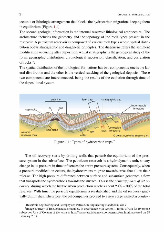
tectonic or lithologic arrangement that blocks the hydrocarbon migration, keeping themin equilibrium (Figure 1.1).The second geologic information is the internal reservoir lithological architecture. Thearchitecture includes the geometry and the topology of the rock types present in thereservoir. A petroleum reservoir is composed of various rock types whose spatial distri-bution obeys stratigraphic and diagenetic principles. The diagenesis refers the sedimentmodification occurring after deposition, whilst stratigraphy is the geological study of theform, geographic distribution, chronological succession, classification, and correlationof rocks ∗.The spatial distribution of the lithological formations has two components: one is the lat-eral distribution and the other is the vertical stacking of the geological deposits. Thesetwo components are interconnected, being the results of the evolution through time ofthe depositional system.
Figure 1.1: Types of hydrocarbon traps †
The oil recovery starts by drilling wells that perturb the equilibrium of the pres-sure system in the subsurface. The petroleum reservoir is a hydrodynamic unit, so anychange in its pressure in time influences the entire pressure system. Consequently, whena pressure modification occurs, the hydrocarbons migrate towards areas that allow theirrelease. The high pressure difference between surface and subsurface generates a flowthat transports the hydrocarbons towards the surface. This is the primary phase of oil re-covery, during which the hydrocarbon production reaches about 20%− 30% of the totalreserves. With time, the pressure equilibrium is reestablished and the oil recovery grad-ually diminishes. Therefore, the oil companies proceed to a new stage named secondary
∗Reservoir Engineering and Petrophysics-Petroleum Engineering Handbook, Vol V†Image courtesy of Encylopaedia Britannica, in accordance with section 1.Terms of Use for Everyone
subsection Use of Content of the terms at http://corporate.britannica.com/termsofuse.html, accessed on 28February 2014.

1.2. DATA ASSIMILATION IN RESERVOIR ENGINEERING 3
recovery. During this phase the pressure system is stressed by injection of water or gasin some of the drilled wells (the injection wells). This injection generates hydrocarbondisplacement and, consequently, their recovery through the other wells (the productionwells). This procedure increases the amount of recovered hydrocarbons, but still notenough, half of the reserves being still trapped in the formation. After a while, the in-jected water reaches the production wells, which decreases the amount of hydrocarbonsrecovered. When the water injection is no longer economically profitable (the amountof hydrocarbons does not cover the costs with water injection), the oil companies havetwo options: either close the production, or pass to a further phase named tertiary oil re-covery or enhanced oil recovery (EOR). During this phase, complex chemicals or steamare injected in order to change the properties of the fluids and the rocks for an easy flowof the hydrocarbons.The hydrocarbon displacement, during exploitation, generates a flow which followstrajectories that depend on the spatial distribution of the petrophysical properties (e.g.porosity, permeability, water saturation, relative permeability) of the lithological struc-tures present in reservoir. The spatial distribution of the petrophysical properties is re-lated to the spatial distribution of the rock bodies that form the reservoir geology, dif-ferent rock types, usually have different petrophysical properties. Only locally, certainlithological units may have comparable petrophysical properties. For example, crevassesplays may have, locally, comparable petrophysical properties with channel belts. Theserock bodies, distinguished by petrophysical properties and mineralogy are called facies.Consequently, any production optimization plan or field development plan must takeinto account the reservoir geology. A better description of the reservoir geological ar-chitecture improves the geological simulation model, which is the foundation of thedecision-making process.
1.2 Data assimilation in reservoir engineering
Even though the geological simulation model is well calibrated to generate geologicallyplausible realizations, theirs predictions (e.g. the simulated production outcome) are notnecessary, close to the real production data. A field development plan, as part of thedecision-making process, is based on plausible geological realizations whose simulatedmeasurements predicts "well enough" the reality. These predictions are obtained cou-pling the geological model with a numerical model that simulates the reservoir behaviorunder established conditions (given geology, wells positions, well controls etc.). Undergiven well controls, the predictions depend on the initial state of the dynamical variables(pressures and saturations), petrophysical parameters (permeability, porosity, relativepermeability, etc.) and properties of the fluids and/or gas present in reservoir (viscosity,density). A reservoir is located thousands of meters underground and its measurements
4 CHAPTER 1. INTRODUCTION
are sparse and either contains little spatial information or does not contain spatial in-formation at all. This causes a high uncertainty during simulation using the geologicalmodel. Consequently, the initial conditions of the numerical model lie in a sea of un-certainty, which makes it almost impossible to compute estimation of future productionclose to reality. In order to obtain plausible geological realizations with high predictivecapacity, a solution would be to use the data assimilation techniques. Data assimilationis a methodology that incorporates measurements into the mathematical model of thesystem. The purpose of this methodology is to calibrate the state of the system such thatthe model can simulate observations in the closest proximity of the measurements. Indata assimilation, the period of time when the measurements are used for calibration iscalled the assimilation period. When the methodology is used for the dynamical variableestimation, we name the data assimilation procedure state estimation; when the method-ology is used for the calibration of model parameters (static variables), we call it inversemodeling procedure (or parameter estimation).In reservoir engineering the data assimilation is called history matching (HM) and ithas been traditionally used to calibrate the model parameters, such that the simulatedproduction response closely reproduces reservoir past behaviour. Initially, within thehistory matching framework, the model parameters were adjusted manually and, con-sequently the methodology was named manually history matching. In this case, themodel parameters considered were the petrophysical properties of the rock types presentin the reservoir. Nowadays, for the parameter calibration, complex procedures that in-volve developing of automatic routines are used and the methodology is named AssistedHistory Matching (AHM).In the last two decades, many AHM algorithms were proposed (Aanonsen et al 2009,Oliver and Chen 2011, Oliver et al. 2008). Depending on the mathematical proceduresused, one may distinguish two directions: gradient based and gradient free methodolo-gies. The gradient based methodology defines an analytical function that is to be opti-mized. The simplest way to introduce a parameter calibration within a such procedure isachieved through a function that describes the square of the Euclidian distance betweenthe simulated measurements and the reservoir observations (Oliver et al 2008). How-ever, the measurements are contaminated with errors, so the pure euclidian distance istraditionally replaced with a weighted regularized least-square function. The minimiza-tion involves the use of gradients. Various types of algorithms were proposed to solvethe minimization problem (basically, the gradient calculus), either involving the adjoints(Chen et al.(1974), Zhang and Reynolds (2002)) or approximations of the gradients usingNewton-like methods (Oliver et al. 2008). The gradient free methodologies can be cate-gorized according to Sarma et al. (2007) in stochastic algorithms (gradual deformationmethod Roggero and Hu (1998), Hu and Ravalec (2004), Gao et al. (2007), probabilityconditioning method Hoffman and Caers (2006)), streamline based techniques (Vasco
1.3. GEOLOGICALLY CONSISTENT DATA ASSIMILATION 5
and Datta-Gupta (1997), (1999)) and Kalman filter approaches. In Chapter 3 we offer adetailed description of the Kalman filter methodology, together with an overview of theensemble based methods introduced in the Kalman filtering framework.
Irrespective of the assisted history matching algorithm used, the result of the estima-tion process must satisfy a few requirements:
• To predict the future behaviour of the reservoir in existing and new wells withincreased confidence.
• To maintain geological acceptability.
• To incorporate (condition on) all quantifiable information (seismic, gravity, welllogs etc.)
In addition, when possible, the AHM method must offer an uncertainty quantification.The preservation of the geological plausibility during the AHM process is still a
challenge and it is the main goal of this work. The geology is very complex, and its ac-ceptance preservation, when optimization procedures are performed, has been obtainedonly in few particular cases for synthetic reservoirs, and under particular assumptionsregarding the geology simulation. A general AHM method, that is capable to preservethe geology requirements (geometry and topology) when applied, does not yet exist.
1.3 Geologically consistent data assimilation
One of the main problems still associated with the use of data assimilation methodsfor history matching of reservoir models is the lack of geological realism in updates.The assumption is that reservoir models which are geologically plausible and matchall available data are better (i.e. give better predictions) than models which are notgeologically realistic or do not match all data. In the normal workflow, the changesto the properties of reservoir models (like porosity and permeability) introduced by thehistory matching process are usually not consistent with geological knowledge about thereservoir, so that the optimal reservoir model is not achieved. Roughly speaking, thereare three possible ways to solve these problems.
1. First, the parameters of the models used to generate the geological models areadjusted instead of the properties themselves. An example is the probability per-turbation method (Hoffman and Caers, 2004) where the settings of the geolog-ical model used for generating realizations are estimated. Another example isa method implemented by Hu et al. 2012 where the parameters incorporatedin the multi-point geological simulation model are calibrated within ensemble
6 CHAPTER 1. INTRODUCTION
based AHM process. These methods can guarantee realistic geology, but gen-erally achieve a worse fit to the production data.
2. The second option is to estimate the properties while retaining the relevant geo-logical input, for example by retaining multi-point statistics. More fundamentalgeological input, like the topological ordering of facies or layers, may still be lostin such an approach. Examples for the second approach are the Gaussian mix-ture models (Dovera and Della Rossa, 2011) for retaining multi-point statistics,discrete cosine transform (DCT, Jafarpour and McLaughlin 2007) for preservingpatterns similar to image processing, wavelets (Jafarpour 2010) or Kernel PCA(Caers 2004, Sarma et al 2008, Sarma and Chen 2009) based on a projection ofthe log-permeability (the property of interest) into a high dimensional space basedon kernel functions.
3. The third option is an intermediate solution in which the distribution of the faciesis estimated explicitly, using appropriate parameterizations of the facies fields.Also here arises a question whether geological acceptability is preserved. Ex-amples for the third approach are the truncated pluri-Gaussian method (Liu andOliver, 2005), the level set method (David Moreno 2009), the gradual deformationmethod (Hu et al. 1998, 2004), parameterizations using distance fields (Lorentzenet al 2012) or using level-set type functions (Chang et al 2010).
Although the first method is intuitively appealing, some major problems are associ-ated with it. The main problem is the strong non-linearity and lack of sensitivity betweenthe parameters of the models generating the geological instances and the production data.This means that an approach where the geological model parameters are adjusted basedon a mismatch between model predictions and observations are difficult to apply.An important question for the second method is what should be preserved in the assim-ilation step. It is not straightforward which parameters are important in describing ge-ology and, more specifically, the geological features important for reservoir simulation.The third method has the disadvantage that the production data can be rather insensi-tive to boundaries between facies, which are thus hard to estimate. The question alsoarises whether the properties of the facies need to be estimated jointly with the faciesdistribution. Finally, it may not always be possible to describe the reservoir using a fa-cies distribution, especially in the case of gradual transitions between facies or complexfine-scale distributions of the facies.
1.4. RESEARCH OBJECTIVES 7
1.4 Research objectives
The goal of this project is to investigate methods currently being used in the third cate-gory and identify the most promising one. One of these methods should be further devel-oped and tested on a geologically realistic reservoir model. The question which methodpreserves the prior geological information in the best way, depends on two parts: howthe geology is better described and how well the chosen parameters are calibrated bythe data assimilation method. The first part is case dependent. Therefore, two differentgeological simulation models are used for the construction of the internal geometry andtopology of the reservoir. For both geological simulation models, appropriate parame-terizations should be found such that the AHM method chosen to provide geologicallyplausible updates.
1. The first geological simulation model is based on two point statistics and is de-fined in the context of plurigaussian simulation, either by a truncation scheme orby a pure simulation using spatially correlated Gaussian variables. In this case theparametrization is made straightforward by the Gaussian fields themselves. Weaim to introduce appropriate settings of the geological model so that the simu-lated facies instances are geologically plausible and conditioned to all availablemeasurements.
2. The second geological simulation model is based on multi-point geostatistical sim-ulation (MPS). Here, complex curvilinear structures (as channels) can be success-fully generated from conceptual geological models (training images). The MPSmodel has the advantage to generate facies instances with increased geologicalacceptability, but for their direct estimation a suitable parametrization is needed.Consequently, we aim to introduce a new parametrization of the facies fields cou-pled with an appropriate AHM method to drive the estimation process towards therequirements presented.
Besides the estimation purpose, by using ensemble based methods for data assimilation,we aim to offer an uncertainty quantification of the facies distribution. This is crucialwhen reservoir optimization production plans are investigated taking into account thegeological uncertainties. The estimation of uncertainties in the structural model (theboundaries between layers, faults, external reservoir geometry) and the introduction ofthese uncertainties as updatable parameters in the AHM method are not addressed in thisproject.
8 CHAPTER 1. INTRODUCTION
1.5 Thesis outline
The thesis is organized as follows:
• In Chapter 2 we describe the geological simulation models used in this project. Wepresent also the mathematical instruments required for defining the methodologyof each geological simulation model.
• Chapter 3 is dedicated to the data assimilation methodology. We describe theensemble based methods used for history matching.
• In Chapter 4 we present the probabilistic parametrization of the facies fields.Based on this parametrization, we build a geological simulation model whichis further coupled with the ensemble Kalman filter (EnKF) as data assimilationmethod. We place this geological simulation model in the large family of pluri-gaussian simulation models. We provide an estimator of the reference facies fieldtogether with its associated uncertainty quantification. This chapter is based onSebacher et al. 2013.
• In Chapter 5 we describe a geological simulation model by means of which theplurigaussian simulation is conditioned to facies probability maps. The name ofthe model is the Adaptive Plurigaussian Simulation (APS). We couple the geo-logical simulation model with EnKF, as history matching method, for the geologyuncertainty quantification. This chapter is based on an article submitted to Com-putational Geosciences.
• Chapter 6 is dedicated to channelized reservoirs. In this chapter we define a newparametrization of the facies fields, in the context of MPS geological simulationmodel, which is coupled with the EnKF and the iterative adaptive Gaussian mix-ture (IAGM). We perform the experiments on two reservoir models with differentcomplexity. This chapter is based on the article submitted to Computational Geo-sciences.
• In Chapter 7 we present the performance of the APS model in the case of a realfield application for a reservoir located in the North Sea. This chapter is based onan article presented at the 76th EAGE Conference and Exhibition 2014 (Hanea etal. 2014).
• In Chapter 8 we present the conclusions of this study and some recommendationsregarding a possible continuation of this work.
Chapter 2
Geological Simulation Models
2.1 Truncated plurigaussian simulation (TPS)
The main ingredient for the plurigaussian truncation methodology consists of the Gaus-sian random field. Consequently, before presenting the (geological) simulation model,we will first give an introduction to random field theory with a focus on a particularshape e.g. the Gaussian random field. The second ingredient of the simulation modelis the truncation scheme (map). This is introduced in the second subsection, where thesimulation model is presented together with some illustrative examples.
2.1.1 The Gaussian random fields
Definition: Let (Ω, F, P ) be a probability space and T ⊆ Rd (d ≥ 1, integer), a param-eter set. A random field is a function Y : T × Ω → Rm, such that Yt = Y (t, ·) (e.g.Yt(ω) = Y (t, ω), for ω ∈ Ω) is a Rm-valued random variable on (Ω, F, P ), for everyt ∈ T .In the following, we develop the theory for the particular casem = 1, which correspondsto real valued random fields. Consequently, for T ⊆ Rd we can define a random field Yas a function such that Yt are random variables for any t ∈ T . The dimension d of thereal space which includes T gives the dimension of the random field. A one-dimensionalrandom field is usually called a stochastic process. The random fields in two or threedimensions are often encountered in earth sciences, such hydrology or geology, wherespatial correlations of the values of some parameters are needed. Additionally, randomfields are often used in meteorology to model space-time dependent variables.
Let be Y a real valued random field with parameter set T ⊆ Rd (d ≥ 1). Usually,this random field is written as Yt, t ∈ T. For any choice of the positive integer k and
9

10 CHAPTER 2. REVIEW OF GEOLOGICAL SIMULATION MODELS
of the finite set of parameters t1, t2, . . . , tk from T , we define the function,Ft1,t2,...,tk : R
k → [0, 1], where R = R ∪ −∞,∞
Ft1,t2,...,tk (x1, x2, . . . , xk) = P (Yt1 ≤ x1, Yt2 ≤ x2, . . . , Ytk ≤ xk) (2.1)
such that, Ft1,...,tk(x1, . . . ,−∞, . . . , xk) = 0 and Ft1,...,tk(∞, . . . ,∞) = 1
We call these functions the finite-dimensional (cumulative) distribution functions (f.d.d.functions) of the random field Y . These functions have two important properties, sym-metry and compatibility.
1. Symmetry: For any permutation σ of the set 1, 2, . . . , k, and for any elementsti ∈ T, i ∈ 1, k we have
Ft1,t2,...,tk = Ftσ(1),tσ(2),...,tσ(k) (2.2)
2. Compatibility: For any k − 1 elements ti ∈ T, i ∈ 1, k − 1 and for any realnumbers xi, i ∈ 1, k − 1 we have
Ft1,t2,...,tk−1(x1, x2, . . . , xk−1) = Ft1,t2,...,tk−1,tk (x1, x2, . . . , xk−1,∞) (2.3)
These properties hold because the values of the f.d.d. functions are probabilities cal-culated for the same events of the probability space (Ω, F, P ). Related with these twoproperties is the Kolmogorov theorem which emphasise the importance of the f.d.d.functions in the context of the existence of the random fields.Kolmogorov existence theorem∗
If a system of probability measures denoted Ft1,t2,...,tk (ti ∈ T ⊆ Rd) satisfies thesymmetry conditions and the compatibility conditions, there exists a probability space(Ω, F, P ) and a random field defined on it, having Ft1,t2,...,tk as its finite-dimensionaldistribution functions.This theorem gives the necessary and sufficient conditions for the random fields exis-tence. Based on this theorem, we will introduce Gaussian random fields. Before that,we introduce the first two moments associated with the random fields.
1. The expectation (mean) function: m : T → R
m(t) =
∫R
x dFt(x) = E(Yt) (2.4)
∗Abrahamsen P., A review of Gaussian Random Fields and Correlation Functions, 1997

2.1. TRUNCATED PLURIGAUSSIAN SIMULATION (TPS) 11
2. The covariance function: C : T 2 → R
C(t1, t2) = Cov(Yt1 , Yt2) = E((Yt1 −m(t1))(Yt2 −m(t2)))
=
∫∫R2
xy dFt1,t2(x, y)−m(t1)m(t2) (2.5)
For the random fields characterized by continuous variables, the f.d.d. functions can bedefined by the probability density functions (pdf ). These functions can be calculated aspartial derivatives of the f.d.d functions.
pt1,...,tk (xt1 , . . . , xtk ) =∂kFt1,...,tk (x1, . . . , xk)
∂x1 . . . ∂xk(2.6)
We can write the mean function and the covariance function with respect to the probabil-ity density functions. m(t) =
∫R x pt(x) dx and C(t1, t2) =
∫∫R2 xy pt1,t2(x, y) dx dy.
In addition, if we denote by σ(t) =√C(t, t) we can define the (auto) correlation
function:
ρ(t1, t2) =C(t1, t2)
σ(t1)σ(t2)(2.7)
Note that the definition of the correlation function is correct, since C(t, t) > 0.Random fields propertiesWe have defined the random fields with no restrictions for the parameter space T. How-ever T ⊆ Rd, and Rd has a structure of an Euclidian space. When T borrows propertiesfrom Rd (the linear structure or the Euclidian structure) we can describe special classesof random fields. These classes are defined through properties that the f.d.d. or meanand covariance functions may have. These properties refer to the invariance of f.d.d.functions to some transformations of the space T.
• Stationarity (Homogeneity)Definition: A random field Y is said to be strictly stationary (or homogeneous)if its finite-dimensional distributions are invariant under a space translation of thelinear space T .That is, if we consider the translation φτ : T → T , φτ (t) = t + τ then thestationarity property can be written as
Ft1,t2,...,tk (x1, x2, . . . , xk) = Fφτ (t1),φτ (t2),...,φτ (tk)(x1, x2, . . . , xk) (2.8)
Consequently, for stationary random fields the mean function is constant on thespace T (m(t) = m for every t ∈ T ), whereas the covariance function can bedefined one-dimensional as C(t1, t2) = C(τ), where τ = t2 − t1. This holdsbecausem(t) =
∫R x dFt(x) =
∫R x dF0+t(x) =
∫R x dF0(x) = m(0) and∫∫
R2 xy dFt1,t2(x, y) =∫∫
R2 xy dF0+t1,(t2−t1)+t1(x, y) =∫∫
R2 xy dF0,t2−t1(x, y)

12 CHAPTER 2. REVIEW OF GEOLOGICAL SIMULATION MODELS
In addition, the correlation function can be written as
ρ(t1, t2) =C(t2 − t1)
σ(t1)σ(t2)=C(t2 − t1)
σ(0)2= ρ(t2 − t1) (2.9)
hence, C(t1, t2) = C(t2 − t1) = σ(0)2ρ(t2 − t1)
When only the mean function and the covariance function are invariant to anyspace translation the random field Y is called weakly stationary.
• IsotropyFor the definition of the isotropy, besides the linear characterization of the spaceparameter T ⊆ Rd we consider the Euclidian structure of the space Rd. Thismeans that we can calculate the Euclidian distance between any two point t1 andt2 from T , using the formula:
d(t1, t2) =
√√√√ d∑j=1
(tj1 − tj2)2
Definition: A stationary random field Y is said to be isotropic if its covariancefunction depends only on the euclidian distance. That is,C(t1, t2) = C(d(t1, t2)).One can observe that the isotropic random fields are invariant to the translationsand rotations of the parameter space T , and therefore to its isometries.
• AnisotropyLet us consider a positive semi-definite symmetric matrix B ∈ Md(R). Then thefunction ‖ · ‖B: Rd → Rd, ‖ t ‖B=
√tTB t is a norm in the euclidian space Rd,
named B-norm.Definition: A stationary random field Y is said to be anisotropic if its covariancefunction depends on the distance defined based on the B-norm.That is, C(t1, t2) = C(‖ t2 − t1 ‖B) .We extend the anisotropy property for the bi-dimensional case (d=2). Using anorthogonal transformation of the space R2 the semi-positive defined matrix B canbe adjusted to its diagonal form. That is, B = ΛT BΛ where B = diag(a, b) isthe diagonal form of the matrix B. Because of the semi-positive definiteness ofthe symmetric matrix B, a and b are non-negative real numbers. The directions ofthe two eigenvectors of the matrix B give the principal and secondary anisotropydirections. The principal direction is given by the eigenvector that corresponds tothe higher eigenvalue, whereas the secondary direction is given by the eigenvectorthat correspond to the lower eigenvalue. One can notice that the two eigenvectorsare orthogonal to each other due the symmetry of the matrix B.
2.1. TRUNCATED PLURIGAUSSIAN SIMULATION (TPS) 13
Gaussian random fieldsDefinition: A Gaussian random field is a random field for which finite-dimensional
distributions Ft1,t2,...,tk are multivariate Gaussian distributions for any choice of thenumber k and the parameters t1, t2, . . . , tk from the space T.If the f.d.d. functions are consistently defined (satisfying the conditions of the probabil-ity measure), the Kolmogorov’s hypotheses are fulfilled and, consequently the definitionof the Gaussian random field is correct. A cumulative distribution function of a mul-tivariate Gaussian variables is defined by its probability density function (pdf ). In themultivariate Gaussian case the pdf is written as:
pt1,t2,...,tk(x1, x2, . . . , xk) =1√
2π | Σt1,t2,...,tk |e−
12
(x−m)TΣ−1t1,t2,...,tk
(x−m) (2.10)
where, x = (x1, x2, . . . , xk) ∈ R and m = (m(t1),m(t2), . . . ,m(tk), m(ti) = E(Yti)
are the expectations. The components of the matrix Σ give the covariances of themarginal variables, e.g. Σt1,t2,...,tk(i, j) = Cov(Yti , Ytj ), for every ti, tj ∈ T . Re-ciprocally, a function pt1,t2,...,tk : Rk → R could be a probability density function of amultivariate Gaussian random variable if and only if the matrix Σt1,t2,...,tk is symmetricand positive definite.
Consequently, the existence of the Gaussian fields is related to the consistent def-inition of the matrices Σt1,t2,...,tk , for any choice of the elements t1, t2, . . . , tk fromT . Since the components of matrices Σt1,t2,...,tk are the covariances Cov(Yti , Ytj ),the Gaussian random fields are well defined by two functions m : T → R and C :
T × T → R. If the function m has no restrictions the function C must be symmetric(C(t1, t2) = C(t2, t1)) and all the square matrices Σt1,t2,...,tk of which components aredefined as Σt1,t2,...,tk(i, j) = Cov(Xti , Xtj ) must be positive definite. The positive def-initeness of the matrices Σ introduces a property for the function C called, as well, thepositive definiteness. Consequently, a function C : T × T → R is said to be positivedefined, if for every positive integer k and for every real numbers αi (1 ≤ i ≤ k) andelements t1, t2, . . . , tk from T , we have
k∑i,j=1
αiαjC(ti, tj) > 0 (2.11)
We will say that, the function C gives the covariance model of the Gaussian randomfield. To prove that a function is positive defined is a tedious process that involves theuse of the Fourier transform (see Christoakos 1984,1992) and is not discussed in this in-troductory section. However, the finite sum or product of acceptable covariance modelsis an acceptable covariance model (satisfies the positive definiteness property, Chris-toakos 1992).In the following, we present some of the underlying covariance models that are used
14 CHAPTER 2. REVIEW OF GEOLOGICAL SIMULATION MODELS
for defining stationary Gaussian random fields (isotropic or anisotropic). We will usethese models in the next section where the truncated plurigaussian simulation model ispresented.
Examples of covariance models:
(1) Spherical model: C(τ) =
σ2
0(1− 32( τh) + 1
2( τh)3) if 0 ≤ τ < h
0 if τ ≥ h
(2) Exponential model: C(τ) = σ20e− 3τh , for τ ≥ 0
(3) Gaussian model: C(τ) = σ20e− 3τ2
h2 , for τ ≥ 0
In geosciences, the term variogram model is commonly used instead of covariancemodel. The variogram of a random field Y is defined as γ(t1, t2) = 1
2V ar(Yt1 − Yt2).For a stationary random field one may write γ(t1, t2) = 1
2E((Yt1 − Yt2)2) and it can beshown that γ(t1, t2) = C(0)−C(t2−t1), whereC(t1, t2) = C(t1−t2) is the covariancemodel. Consequently, for a stationary random field the variogram depends on the differ-ence t2 − t1, γ(t1, t2) = γ(t2 − t1) like the covariance does, and γ(τ) = C(0)− C(τ)
(Kelkar and Perez 2002). The variogram behaves complementary to the covariance. Forexample, when we use decreasing covariance models (like the ones presented above) forincreasing lag-distance τ the variogram increases from zero towards σ2
0 . The parame-ter h that occurs in the definition of the covariance models presented before is named"the range" of the covariance model (or variogram model). From the covariance modelperspective, when the distance τ exceeds value h the covariance is zero (for sphericalmodel) or almost zero (for the other models).
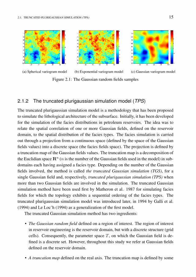
The plurigaussian truncation model uses Gaussian fields defined on discrete param-eter sets. To generate samples (values) of the Gaussian random fields, when the setof parameters is finite, one may use, for instance the sequential Gaussian simulationmethod (Kelkar and Perez 2002) or the moving averages method (Oliver 1995). Forthat, we have to set up the geostatistical properties of the Gaussian field e.g. the meanfunction, the variance function, the covariance (variogram) model type, the correlationdirection, and the directional correlation ranges. In the Figure 2.1 we present three sam-ples of stationary Gaussian random fields defined on the finite set 1, 2, . . . , 1002. Themean model is equal to 0 and the variance model is equal to 1. The Gaussian randomfields were chosen to have the isotropic property with a range of 20. The variogram mod-els used in this example were the spherical (sub-figure (a)), exponential (sub-figure (b))and Gaussian(sub-figure (b)). The samples were carried out using the sequential Gaus-sian simulation method implemented in S-GeMS (The Stanford Geostatistical ModelingSoftware).
2.1. TRUNCATED PLURIGAUSSIAN SIMULATION (TPS) 15
(a) Spherical variogram model (b) Exponential variogram model (c) Gaussian variogram model
Figure 2.1: The Gaussian random fields samples
2.1.2 The truncated plurigaussian simulation model (TPS)
The truncated plurigaussian simulation model is a methodology that has been proposedto simulate the lithological architecture of the subsurface. Initially, it has been developedfor the simulation of the facies distributions in petroleum reservoirs. The idea was torelate the spatial correlation of one or more Gaussian fields, defined on the reservoirdomain, to the spatial distribution of the facies types. The facies simulation is carriedout through a projection from a continuous space (defined by the space of the Gaussianfields values) into a discrete space (the facies fields space). The projection is defined bya truncation map of the Gaussian fields values. The truncation map is a decomposition ofthe Euclidian space Rn (n is the number of the Gaussian fields used in the model) in sub-domains each having assigned a facies type. Depending on the number of the Gaussianfields involved, the method is called the truncated Gaussian simulation (TGS), for asingle Gaussian field and, respectively, truncated plurigaussian simulation (TPS) whenmore than two Gaussian fields are involved in the simulation. The truncated Gaussiansimulation method have been used first by Matheron et al. 1987 for simulating faciesfields for which the topology exhibits a sequential ordering of the facies types. Thetruncated plurigaussian simulation model was introduced later, in 1994 by Galli et al.(1994) and Le Loc’h (1994) as a generalization of the first model.
The truncated Gaussian simulation method has two ingredients:
• The Gaussian random field defined on a region of interest. The region of interestin reservoir engineering is the reservoir domain, but with a discrete structure (gridcells). Consequently, the parameter space T , on which the Gaussian field is de-fined is a discrete set. However, throughout this study we refer at Gaussian fieldsdefined on the reservoir domain.
• A truncation map defined on the real axis. The truncation map is defined by some
16 CHAPTER 2. REVIEW OF GEOLOGICAL SIMULATION MODELS
thresholds that divide the real axis into intervals, each having assigned a faciestype.
If we consider the reservoir domain D, in two or three dimensions, and a number of kfacies types that occur in the domain, then the regions occupied by the facies type j inthe domain D could be described as:
Fj = u ∈ D|sj−1 ≤ Y (u) < sj (2.12)
where Y is a sample of the Gaussian field, Y (u) is the value of of the Gaussian fieldat the location u ∈ D, and sj , j = 0, k are the thresholds that define the truncationmap. We use the convention s0 = −∞ and sk = ∞. The choice of the thresholdsthat define the one-dimensional truncation map is based on the best knowledge about theproportions of the facies types. If we consider propj as being the proportion of the faciestype j, (j = 1, k) then we have the relation between the proportions and the thresholds
propj =
∫ sj
sj−1
pdf(x)dx = cdf(sj)− cdf(sj−1) (2.13)
where pdf and cdf represents the probability density function and, respectively, the cu-mulative distribution function of the normal distribution used for definition of the (sta-tionary) Gaussian field. Using these equations, we find the thresholds as functions ofproportions
sj = cdf−1(
j∑i=1
propi) (2.14)
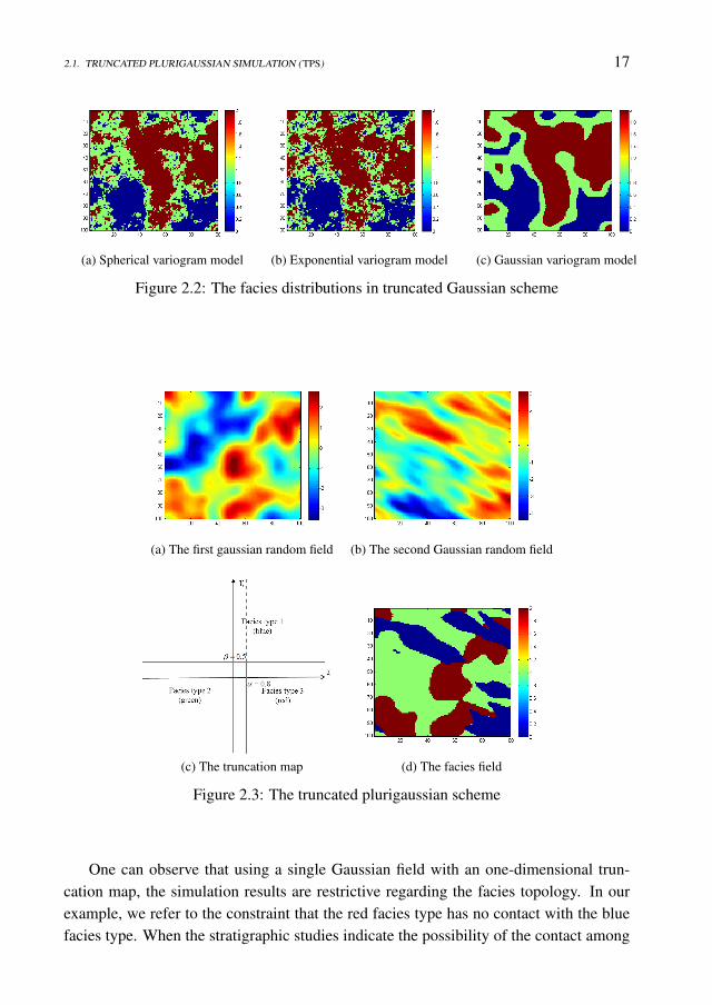
In practice, the facies proportions are estimated using data collected at the reservoirexploration phase. However, the indicator facies proportions has two components. Oneis the global indicator facies proportions and represents the proportion of each faciestype in entire reservoir domain. Based on the values of this indicator one may definethe thresholds described by the equations 2.14. The second meaning refers to a kind ofspatial distribution of this indicator. The studies related with the lateral distribution ofthe geological deposits may conclude that in different regions of the reservoir domainthe facies types may have different proportions. This means that we deal with spatialnon-stationarity in facies proportions. In this case the values of the thresholds vary withthe location in the domain (Galli et al 1997).In Figure 2.2 we present three examples of facies fields obtained after truncation of theGaussian fields presented in the Figure 2.1. For that, we have defined two thresholdss1 = −0.4 and s2 = 0.8 on the real axis and assign to each interval, a facies type. Theblue facies type is assigned for the Gaussian field values less than -0.4, the green faciestype for the values between -0.4 and 0.8 and the red facies type for the values greaterthan 0.8.
2.1. TRUNCATED PLURIGAUSSIAN SIMULATION (TPS) 17
(a) Spherical variogram model (b) Exponential variogram model (c) Gaussian variogram model
Figure 2.2: The facies distributions in truncated Gaussian scheme
(a) The first gaussian random field (b) The second Gaussian random field
(c) The truncation map (d) The facies field
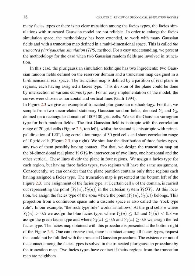
Figure 2.3: The truncated plurigaussian scheme
One can observe that using a single Gaussian field with an one-dimensional trun-cation map, the simulation results are restrictive regarding the facies topology. In ourexample, we refer to the constraint that the red facies type has no contact with the bluefacies type. When the stratigraphic studies indicate the possibility of the contact among
18 CHAPTER 2. REVIEW OF GEOLOGICAL SIMULATION MODELS
many facies types or there is no clear transition among the facies types, the facies sim-ulations with truncated Gaussian model are not reliable. In order to enlarge the faciessimulation space, the methodology has been extended, to work with many Gaussianfields and with a truncation map defined in a multi-dimensional space. This is called thetruncated plurigaussian simulation (TPS) method. For a easy understanding, we presentthe methodology for the case when two Gaussian random fields are involved in trunca-tion.
In this case, the plurigaussian simulation technique has two ingredients: two Gaus-sian random fields defined on the reservoir domain and a truncation map designed in abi-dimensional real space. The truncation map is defined by a partition of real plane inregions, each having assigned a facies type. This division of the plane could be doneby intersection of various curves types. For an easy implementation of the model, thecurves were chosen as horizontal and vertical lines (Galli 1994).In Figure 2.3 we give an example of truncated plurigaussian methodology. For that, wesample from two uncorrelated stationary Gaussian random fields, denoted Y1 and Y2,defined on a rectangular domain of 100*100 grid cells. We set the Gaussian variogramtype for both random fields. The first Gaussian field is isotropic with the correlationrange of 20 grid cells (Figure 2.3, top left), whilst the second is anisotropic with princi-pal direction of 120, long correlation range of 30 grid cells and short correlation rangeof 10 grid cells (Figure 2.3, top right). We simulate the distribution of three facies types,any two of them possibly having contact. For that, we design the truncation map onthe bi-dimensional real plane Y1OY2 by intersection of two lines, one horizontal and theother vertical. These lines divide the plane in four regions. We assign a facies type foreach region, but having three facies types, two regions will have the same assignment.Consequently, we can consider that the plane partition contains only three regions eachhaving assigned a facies type. The truncation map is presented at the bottom left of theFigure 2.3. The assignment of the facies type, at a certain cell u of the domain, is carriedout representing the point (Y1(u), Y2(u)) in the cartesian system Y1OY2. At this loca-tion, we assign the facies type of the zone where the point (Y1(u), Y2(u)) belongs. Thisprojection from a continuous space into a discrete space is also called the "rock typerule". In our example, "the rock type rule" works as follows. At the grid cells u whereY2(u) > 0.5 we assign the blue facies type, where Y2(u) ≤ 0.5 and Y1(u) < 0.8 weassign the green facies type and where Y2(u) ≤ 0.5 and Y1(u) ≥ 0.8 we assign the redfacies type. The facies map obtained with this procedure is presented at the bottom rightof the Figure 2.3. One can observe that, there is contact among all facies types, requestthat could not be fulfilled with the truncated Gaussian procedure. The existence or not ofthe contact among the facies types is solved in the truncated plurigaussian procedure bythe truncation map. Two facies types have contact if theirs regions from the truncationmap are neighbors.
2.1. TRUNCATED PLURIGAUSSIAN SIMULATION (TPS) 19
If in the truncated Gaussian case the truncation map is defined by the choice of thethresholds, in the plurigaussian case the truncation map is uniquely defined by the pa-rameters of the curves that describe it. For the rectangular truncation map used in theexample, these parameters consist of two values: one situated on the horizontal axis (α)and the other on the vertical axis (β). They are calculated, like in the first case, basedon the best knowledge about the facies proportions. The difference is that, now, twoGaussian random fields are involved; therefore the problem related with the correlationbetween them occurs. If we denote by Dj the region from the truncation map assignedto the facies type j, and by propj the proportion of the same facies type, then we havethe relation:
propj =
∫∫Dj
pdf(Z1,Z2)(z1, z2)dz1dz2 (2.15)
where pdf(Z1,Z2) is the probability density function of the multivariate Gaussian variable(Z1, Z2). The marginal variables Z1 and Z2 are Gaussian variables with the distributiondefined by the mean function and variance function of the Gaussian fields Y1 and Y2. Themultivariate Gaussian variable (Z1, Z2) expresses the correlation between the Gaussianfields Y1 and Y2. Finding the parameters of the truncation map requires to solve thesystem of equations given by the relations 2.15 (Armstrong et al 2011).
However, the most complex procedure, when one wants to apply the TPS, is to es-tablish the geostatistical properties of the Gaussian fields and to design the truncationmap such that the simulations reflect as better as possible the reality. This means thatthe facies simulations are geologically acceptable. The geological acceptance refersto obtaining of realistic topology (the relative position among the facies) and geome-try (shape, dimension, number of the facies). When the geostatistical properties of theGaussian fields are set, a realistic topology of the facies simulation is achieved with areliable choice of the truncation map (Lantuejoul 2002). The geometry of the facies isa property controlled by the geostatistical properties of the Gaussian fields. For a giventruncation map, the correlation directions (which give the isotropy or anisotropy) andthe directional correlation ranges of the Gaussian fields can be estimated knowing themathematical relation between the indicator variogram of the facies types and the vari-ogram of the Gaussian fields (Le Loc’h and Galli 1997, Armstrong et al. 2011). A muchsimpler approach is presented by Chang and Zhang (2014). Here the authors proposed atrial and error procedure for the estimation of the geostatistical properties of the Gaus-sian fields.
20 CHAPTER 2. REVIEW OF GEOLOGICAL SIMULATION MODELS
2.2 Multiple-point geostatistical simulation (MPS)
The goal of any geological (geostatistical) simulation model is to provide instances offacies maps (reservoir models) that are able to reflect the best knowledge about the sub-surface geology. When the information gathered indicates the existence of geo-bodieswith defined geometrical shapes (such curvilinear or elliptical structures), the use of geo-logical models based on two-points statistics (variogram) (such TPS) is not suitable. Thereason resides on what a variogram represents. The variogram is a statistical instrumentthat measures the dissimilarity between the same (or different) variable(s) values at twospatial locations. Consequently, a variogram model is limited in capturing geologicalfeatures with defined shapes, it can capture trends but not concepts. For instance, cannotcapture with a simple mathematical formula the geometry of curvilinear features (e.g.channels), although can establish a high correlation in its propagation direction. For thatreason, the TPS model provides various textures of the facies maps, but it cannot keepsa fixed geometry of facies shapes.
To be able to model features with defined shapes, a solution is to use the multiple-point geostatistical simulation models (MPS, Guardiano and Srivastava 1993, Journel1993). The multi-point geostatistical simulation models are geostatistical methodolo-gies that takes into account correlations between many spatial locations at the sametime. These correlations are inferred from conceptual models e.g. training images. De-pending on the variable that has to be modeled, the training image can be discrete (orcategorial, for facies distributions) or continuous (for variables with continuous valuessuch as porosity or permeability).
2.2.1 The (discrete) training image
A (discrete) training image is a conceptual image (in two or three dimensions) designedto reproduce the topology, geometry and the connectivity of the lithological units (facies)from the subsurface e.g. the geological heterogeneity. A training image has a powerfulvisual impact, reflecting a prior geological model, which design is carried out based ongeological interpretation from all available sources (outcrops, sample data, stratigraphicstudies etc.), but without conditioning on any hard or soft data. A training image canbe viewed as library of geometrical patterns that we believe it could be present in thesubsurface. A pattern is a geometrical configuration, extracted from the training image,identifying a possible structure of the spatial continuity. These patterns are incorporatedin the training image and reciprocally the training image is an assemblage of the patterns.
In the traditional MPS methodology, not any image that describe a type of geologicalheterogeneity could be a training image. To be used as training image, a conceptualimage must satisfy some requirements.
2.2. MULTIPLE-POINT GEOSTATISTICAL SIMULATION (MPS) 21
1. StationarityThis property refers to the stationarity of the geometrical patterns that composethe training image. The goal of the MPS method is to generate facies maps withpatterns borrowed from the training image. In the traditional MPS methodology,the simulation is carried out based on sampling from the empirical multivariateconditional probability density function (cpdf ) of the geometrical templates (multipoint statistics) calculated from the training image. Consequently, reliable faciesmaps are obtained when consistent cpdf are inferred from the training image. Theconsistency of the cpdf is ensured by the repeatability of the geometrical patternswithin training image, coupled with stationarity in the geometry of the patterns(e.g. size and geometry of the elliptical shapes or width when refer to channels).
2. The size of the training imageThe size of the training image should be correlated with the size of the largestpattern that one would simulate within a given reservoir domain. For instance,when channels have to be simulated, the dimension of the training image shouldbe at least twice larger than the dimension of the reservoir domain, in the directionof the channels continuity (Caers and Zhang 2004).
In addition, the number of the categorial variables from the training images should berestricted to maximum five. This is because the numbers of the geometrical templatesincreases exponentially with the number of categories present in the training image anda high number of categories may causes a huge computational effort in calculation andstorage of the cpdf.
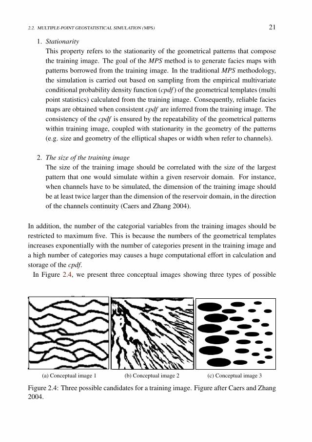
In Figure 2.4, we present three conceptual images showing three types of possible
(a) Conceptual image 1 (b) Conceptual image 2 (c) Conceptual image 3
Figure 2.4: Three possible candidates for a training image. Figure after Caers and Zhang2004.
22 CHAPTER 2. REVIEW OF GEOLOGICAL SIMULATION MODELS
geological heterogeneities; the fluvial type (Image 1), the deltaic type (Image 2) anda conceptual image defined by elliptical shapes (Image 3). From these three images,only the first image fulfills the stationarity request and could be used as training image(for traditional MPS methodologies). One can observe that the deltaic image lacks thestationarity with respect to the width and anisotropy direction of the local patterns. Theconceptual image with elliptical shapes does not keeps the stationarity in the dimensionof the local patterns in space; its patterns are stationary regarding only the shape.
However, in the recent research on the MPS, the concept "training image" has beenrelaxed. New MPS methodologies have been developed to fit to training images that arenot constraint to size and stationarity. Hu et al 2014 uses as training image an existentreservoir, and a new MPS algorithm is developed to simulate facies maps from "non-stationary" training images. The "non-stationary" training image can be built using anytype of reservoir modeling approach. A non-stationary MPS methodology have beendeveloped by Honarkhah and Caers (2012), for creating multiple-point geostatisticalmodels, based on a distance-based modeling and simulation of patterns. The authorsuses a deltaic training image (like Image 2) to present the methodology.
2.2.2 The simulation models
Two of the most commonly used MPS methodologies to simulate categories e.g. faciesdistributions are the SNESIM (single normal equation simulation, Strebelle 2002) andFILTERSIM (filter-based simulation, Zhang et al 2006,).
The SNESIM algorithm is an enhancement of the pioneered MPS algorithm pro-posed by Guardiano and Srivastava in 1993. It consists of two procedures. The firstcalculates, from the training image, the cpdf of the geometrical templates found withina user-defined window search. The second is a procedure that sequentially simulatesa facies type at each grid cell of the reservoir domain. The simulation is based on asample from the cpdf of a geometrical template found in the window centered at thatlocation. The template is formed taking into account hard data (facies observations), ifavailable, and the values at the previous simulated cells from the window. The grid cellof the domain are visited only once, based on a random path apriori given. The noveltyintroduced by Strebelle consists on a procedure for the calculation and the storage ofthe cpdf of the geometrical templates. In the original methodology, the training imagehad to be scanned each time when simulated at unsampled grid cell, which requires anextremely high CPU demanding. The SNESIM calculates the cpdf within a dynamicaldata structure called "search three", by which the training image has to be scanned onlyonce. The dimension of the "search three" depends on the dimension of the window thatscan the training image at the beginning of simulation.
2.2. MULTIPLE-POINT GEOSTATISTICAL SIMULATION (MPS) 23
In the later years the SNESIM procedure has been enhanced, with procedures thatenable the conditioning of the facies simulation not only on the training image and thehard data, but also on probability maps coming from seismic interpretations. This hasbeen done incorporating a probabilistic model named "tau model" in the simulation ofa facies type at unsampled locations (Journel 2002, Krishnan et al. 2005). In addition,various procedures have been incorporated, by which non-stationary facies fields (withnon-stationary geometrical patterns) can be generated started from training images withstationary characteristics (Strebelle and Zhang 2005). However, the SNESIM is limitedregarding to the number of the facies types and is suitable only for discrete training im-ages.
The MPS algorithm FILTERSIM has been proposed to overcome these issues. TheFILTERSIM algorithm is less memory demanding with reasonable CPU cost and canhandle with both discrete and continuous training images (Zhang et al 2006). FILTER-SIM utilizes a set of filters to classify training (geometrical) patterns in a small real spaceof which dimension is given by the number of the filters used (called the filter space). Afilter is a set of weights associated with all the cells of a geometrical template. A tem-plate is a local moving window used to scan the training image providing the trainingpatterns. For a given training pattern each filter gives a score, and consequently eachpattern is associated with a point in a filter space. By adequate partitioning of the filterspace, the patterns are grouped in classes. An average of each class is called prototypefor the patterns. The simulation with the FILTERSIM algorithm is performed in a se-quential manner, using a random path to visit each cell. During simulation, the prototypeclosest to the conditioning data event (which comprises all the informed cells from thetemplate with the center in the visited cell) is determined and a pattern randomly sampledfrom that prototype is pasted onto the simulation cell. As SNESIM, the FILTERSIM canbe conditioned on probability maps inferred from seismic interpretations.
Another MPS algorithm is introduced by Arpat and Caers 2004. This methodologydoes not uses a grid-cell based simulation (as SNESIM) of the categorial variables, buta simulation based on patterns. For that reason the MPS methodology has been namedpattern-based simulation. First, a database of patterns is extracted from a training image.Secondly, the simulation is carried out by pasting at each visited location along a randompath a pattern that is compatible with the available local data and any previously simu-lated patterns. At each step, the reliable pattern is chosen by using a distance functionthat measure the similarity between patterns.
Chapter 3
Ensemble methods
3.1 Data assimilation basics
Data assimilation is a novel methodology for estimating variables representing certainstate of nature. Estimation of a quantity of interest via data assimilation involves com-bining measurements with the underlying dynamical principles governing the systemunder observation. Different problems require knowledge of the distribution and evolu-tion in space and time of the characteristics of the systems involved in each of them. Thefunctions of space and time (state variables or model states) are the ones which char-acterize the state of the system under observation. A dynamical model to describe thenature consists of a set of coupled nonlinear equations for each state variable of interest.The discrete model for an evolution of dynamical system from time tk−1 to time tk canbe described by the equation of the form:
x(tk) =M(x(tk−1), θ) (3.1)
where x(tk) ∈ Rnm denotes the vector of dynamical variables at time tk and θ denotesthe vector of poorly known parameters. Usually, the dynamic operatorM : Rnm+nθ →Rnm is nonlinear and deterministic (nm and nθ are the dimensions of the spaces wherethe variables takes values). So, we are working under the assumption of a perfect model.At each time step tk, the relationship between measured data dobs(tk) and state variablesx(tk) can be described by a nonlinear operator Hk : Rnm+nθ → Rn
dobs . If we assumethat observations are imperfect the simulated measurements are described by
dobs(tk) = Hk(x(tk), θ) + v(tk) (3.2)
where v(tk) is the observation error with v(tk) ∼ N (0,R(tk)). The most importantproperties of the system appear in the model equations as parameters (static variables).
24
3.1. DATA ASSIMILATION BASICS 25
In theory parameters of the system can be estimated directly from measurements. Inpractice, direct measuring the parameters of a complex system is difficult because ofsampling, technical and resource requirements. Data assimilation however provides apowerful methodology for parameter estimation.Given a dynamical model with initial and boundary conditions and a set of measure-ments that can be related to the model state, the state estimation problem is definedas finding the estimate of the model state that fits the best (under a certain criterion)the model equations, the initial and boundary conditions, and the observed data. Theparameter estimation problem is different from the state estimation problem. Tradition-ally, in parameter estimation we want to improve estimates of a set of poorly knownmodel parameters leading to a better model solution that is close to the measurements.Thus, in this case we assume that all errors in the model equations are associated withuncertainties in the selected model parameters. The model initial conditions, boundaryconditions, and the model structure are all considered to be known. Hence, for any set ofmodel parameters the corresponding solution is found from a single forward integrationof the model. One way to solve both problems is to define a cost function that measuresthe distance between the model prediction and the observations plus a term measuringthe deviation of the parameter values from a prior estimate of the parameter values. Therelative weight between these two terms is determined by the prior error statistics for themeasurements and the prior parameter estimate.
J(x) =1
2
∑k
[dobs(tk)−Hk(x(tk))]TR(tk)−1[dobs(tk)−Hk(x(tk))]
+1
2[xp(t0)− x(t0)]TC−1
0 [xp(t0)− x(t0)]
(3.3)
These estimation problems are hard to solve due to nonlinear dynamics of the system aswell as the observational model and due to the presence of multiple local minima in thecost function.The schemes for solving the state and parameter estimation have different backgrounds.They often belong to either control theory or estimation theory. The control theoryuses variational assimilation approaches to perform a global time and space adjustmentof the model solution to all observations. The goal is to minimize the cost function(3.3) penalizing the time-space misfits between the observed data and predicted data,with the model equations and their parameters as constraints (Talagrand and Courtier1987). Results depend on the a priori control weights and penalties added to the costfunction. The dynamical model can be either considered as a strong (perfect model) orweak constraint (in the presence of model error). The variational data assimilation is aconstrained minimization problem, which is solved iteratively with a gradient-based op-timization method. First, the problem is reformulated as an unconstrained minimization

26 CHAPTER 3. REVIEW OF ENSEMBLE METHODS
problem by adding the model equations and constraints to the objective function. Thegradients are then obtained using a so-called adjoint method that allows us to calculateall the sensitivities by only two simulations: one backward using the adjoint and oneforward in time.The estimation theory uses a statistical approach to estimate the state of a system bycombining all available reliable knowledge about the system including measurementsand models. This falls in the Bayesian estimation territory, where we find the Kalmanfilter approach (Kalman [1960]) as a simplification for the case of linear systems. Forlinear models the Kalman Filter is the sequential, unbiased, minimum error variance es-timate based on a linear combination of all past measurements and dynamics. Kalmanfiltering is formulated as sequential estimation procedure, i.e. such that the data areassimilated whenever they become available. The end results will be
• xa(tk) is the optimal estimate of xt(tk) using dobs(t1) . . . dobs(tk)
• Ca(tk) is the covariance matrix of the estimation error,
where the superscript "a" denotes the analyzed state and covariance. These two areobtained by following the classical Kalman filter equations
• The first step, initialization, is specification of an initial distribution for the truestate
xt(t0) ∼ N (xf (t0),Cf (t0)) (3.4)
• The second step, forecast step, is to specify the error between the true state xt(tk+1)
and the model forecast M(tk)xt(tk) which should be described in terms of Gaus-
sian distribution
xt(tk+1) = M(tk)xt(tk) + η(tk) (3.5)
where η(tk) ∼ N (0,Q(tk)) and M represents the Tangent Linear Model (TLM)ofM.Giving the stochastic model 3.5 and the initial condition 3.4, the Kalman filter isable to compute the true state at every time in the future
xf (tk+1) = E[xt(tk+1)] =
= M(tk)xf (tk)
Cf (tk+1) = E[(xt(tk+1)− xf (tk+1))(xt(tk+1)− xf (tk+1))>] =
= M(tk)Cf (tk)M(tk)> + Q(tk) (3.6)
3.2. ENSEMBLE METHODS FOR NONLINEAR FILTERING PROBLEMS 27
• The third step is the analysis step.
xa(tk) = xf (tk) + K(tk)(dobs(tk)−H(tk)xf (tk)) (3.7)
Ca(tk) = E[(xt(tk)− xa(tk))(xt(tk)− xa(tk))>] =
= (I−K(tk)H(tk))Cf (tk)(I−K(tk)H(tk))>
+ K(tk)R(tk)K(tk)> (3.8)
where the choice for K is the minimal-variance gain and H represents the TangentLinear Model (TLM) ofH
K(tk) = Cf (tk)H(tk)>[H(tk)Cf (tk)H(tk)> + R(tk)]−1 (3.9)
It can be shown that for linear systems, and assuming Gaussian measurement andmodel noise, this sequential approach results in exactly the same answers as the varia-tional method. That means that xa = min
xJ(x) (see eq. 3.3) is the same as the Best
Linear Unbiased Estimator (BLUE) from eq.3.7 calculated in the update step of theKalman filter equations.
3.2 Ensemble methods for nonlinear filtering problems
The classical Kalman filter technique is optimal in case of linear models and Gaussiannoise. In reality, the models describing complex physical phenomena tend not to belinear. Therefore, ensemble Kalman Filter (EnKF, Evensen 1997) was introduced andbecame one of the most promising History Matching methodology. This is a MonteCarlo technique where the probability density of the state is represented by an ensem-ble of possible realizations that are simultaneously propagated in time by the non-linearmodel and updated sequentially when observations become available. One of the issuesthat temper with the quality of the EnKF is the finite number of ensemble members.In the literature (Evensen 1997, 2003, 2006, Aanonsen et al. 2009) a unified opinionwas formed, agreeing that 100 ensemble members are sufficiently enough to keep theEnKF computationally feasible, without sacrificing the quality of the updates. There-fore, EnKF represent a solution for bypassing the need for a linear model in the Kalmanfilter framework. However, it cannot overcome the constraint on Gaussian distributionfor the errors. Regardless of the distribution of the prior uncertainties, EnKF has thetendency to provide approximations to the posterior that are too close to a Gaussian dis-tribution.Particle filters (PF) represent a solution for the non-Gaussian assumptions on the errorsstatistics. It belongs to the same ensemble based approaches. In comparison with the
28 CHAPTER 3. REVIEW OF ENSEMBLE METHODS
EnKF, where the ensemble members are equally probable (equal weights), in case of PFthere is a weight associated with each ensemble member (Doucet 2001). The sum ofthese weights is one. Even if the philosophy in the back of the PF is the same as in theEnKF approach (the ensemble is updated using the Bayes’ rule), the update step differs.In case of PF’s the weights are the ones updated by the observations sequentially. It ismathematically proven that the particle filter is the only data assimilation scheme thatproduces a sample from the exact posterior distribution. Nevertheless, there is a limi-tation of this methodology related with the computational time needed when applied tolarge-scale application. Moreover, for a high dimensional state vector, this methodologysuffers from phenomenon known in literature as the curse of dimensionality, i.e. as thedimension of the system increases the largest of the sample weights converges to onein probability (Bengtsson 2008). The consequence is called filter degeneracy, where theposterior distribution is represented by a single point in the state space.A logical step is to combine the strengths of the two above-mentioned approaches: thecomputationally feasibility of the EnKF with the sampling procedure of the PF. Theresult is a hybrid filter, which uses the Kalman filter update step and the weighted cor-rection. Examples of these kinds of filters are EnKF-SIS (Mandel 2009) and Gaussianmixture filters (Bengtsson 2003, Hoteit 2008a). In the later ones, a mixture density (Sil-verman 1986) approximates the prior distribution where each ensemble member formsthe center of a Gaussian density function (a kernel). The mixture densities togetherwith the weights are propagated by the dynamical model and updated accordingly us-ing the Bayes’ rule. Therefore, the mixture filters in their basic form, are also proneto weight degeneration. Hoteit 2008b showed that the EnKF can be reformulated as amixture filter, by using Gaussian kernels and forcing the weights to be uniform. Thelatter requirement can be made more flexible. Following this idea, Stordal et al. 2012introduced a tuning parameter α ∈ [0, 1] such that when α = 0 one obtains the EnKFequally distributed weights, and α = 1 one obtains the weights of the Gaussian mixturefilter. Hence, taking α to be small the weight degeneracy problem is reduced, but takingα > 0 EnKF approximation of the posterior is improved. Consequently, we obtain abetter preservation of the non-Gaussian features of the marginal distributions. The pro-posed approach is adaptive, in the sense that an optimal α is sought at each assimilationstep resulting in an adaptive Gaussian mixture filter (AGM).
3.2. ENSEMBLE METHODS FOR NONLINEAR FILTERING PROBLEMS 29
3.2.1 The nonlinear filtering problem
The nonlinear filtering problem consist of estimating sequentially in time the state, xt,of a nonlinear dynamical system conditioned on some noisy measurements taken on thestate. For the simplicity of our notations in this section we will denote x(tk) by xt,x(tk−1) by xt−1, dobs(tk) by dobst . Let us consider the following nonlinear problem:
xt =Mt(xt−1) + ηt,
dobst = Htxt + vt,(3.10)
We consider the model error ηt known, given by its probability density function, theinitial distribution given by its probability density function p(x0) and the measurementerror which is assumed GaussianN (0,Rt). The solution of the filtering problem is givenby determining the posterior density p(xt|dobs1:t ). That is, the conditional distribution ofthe state xt given the observations dobs1:t , where dobs1:t = (dobs1 , ..., dobst ). At each momentof time t, the state of the system is defined by two conditional probability density func-tions: the prior density p(xt|dobs1:t−1) and the posterior density p(xt|dobs1:t ). At the initialmoment, where no measurements are available, the probability density function p(x0) isconsidered the posterior. Given the posterior density at time t − 1, the prior density attime t can be calculated using the Chapman-Kolmogorov equation (Jazwinsky 1970)
p(xt|dobs1:t−1) =
∫p(xt|xt−1)p(xt−1|dobs1:t−1)dxt−1. (3.11)
When a new observation dobst occurs, the posterior density is calculates using the Bayesinversion scheme:
p(xt|dobs1:t ) =p(dobst |xt)p(xt|dobs1:t−1)
p(dobst |dobs1:t−1), (3.12)
where the term p(dobst |dobs1:t−1) can be calculated using the relation:
p(dobst |dobs1:t−1) =
∫p(dobst |xt)p(xt|dobs1:t−1)dxt.
However, the probability density functions p(xt|dobs1:t ) (eq.3.12) cannot be computed an-alytically. Consequently, we need to find approximate solutions for these probabilitydensity functions. A simple approach is the use of a Monte Carlo methodology, wherethe prior and posterior densities are approximated with a random sample. Having toapproximate two types of densities (the prior densities and the posterior densities), weuse different notations for samples. We denote by the set of particles xitNi=1 a sam-ple approximating the prior density (3.11) and by the set of particles xitNi=1 a sampleapproximating the posterior density (3.12).

30 CHAPTER 3. REVIEW OF ENSEMBLE METHODS
3.2.2 The ensemble Kalman filter
The ensemble Kalman filter EnKF (Evensen 1994) is a sequential Monte Carlo method-ology introduced in the Kalman filter framework that aims to provide approximate solu-tions to the nonlinear filtering problem.For a given a sample, xit−1Ni=1, from the posterior density p(xt−1|dobs1:t−1), a samplefrom the prior density p(xt|dobs1:t−1) is obtained in the EnKF methodology by samplingfrom the forward density p(xt|xit−1) using eq. (3.10), for each i ∈ 1 . . . N.
xit =Mt(xit−1) + ηit, i = 1, . . . , N. (3.13)
where ηit, for i ∈ 1, . . . , N is a sample from N (0, Qt).If the density p(xt|dobs1:t−1) is Gaussian with mean µt and covariance matrix Ct, it followsthat all the densities from equation 3.12 are Gaussian. First, the observation operator hasGaussian error, therefore the densityp(dobst |xt) = pvt(d
obst −H(t)xt) (Jazwinsky 1970) is Gaussian. Secondly, the normal-
izing term can be written as:
dobst |dobs1:t−1 = H(t)xt|dobs1:t−1 + vt (3.14)
being Gaussian.Consequently, the mean µt and covariance matrix Ct of the conditional variable
xt|dobs1:t are given by the standard Kalman filter update,
µt = µt + Kt(dobst −Htµt),
Ct = (I−KtHt)Ct,
Kt = CtHTt (HtCtH
Tt + Rt)
−1.
(3.15)
Using the relation 3.13 an ensemble xit|i ∈ 1, . . . , N of samples from the priordensity p(xt|dobs1:t−1) is obtained. The mean calculated from this ensemble is an estimatorfor µt and is given by the following formula:
µt ≈ xt =1
N
N∑i=1
xit, (3.16)
If xitNi=1 are samples from the posterior density p(xt|dobs1:t ), then
µt ≈1
N
N∑i=1
xit (3.17)
Combining eq. 3.15 and eq. 3.16, we obtain:
µt = µt + Kt(dobst −Htµt) ≈
1
N
N∑i=1
(xit + Kt(dobst −Htx
it)) (3.18)
If we replace the covariance Ct with the empirical covariance matrix Ct (calculatedfrom the ensemble xit|i ∈ 1, . . . , N) in the calculus of the Kalman gain Kt (eq.
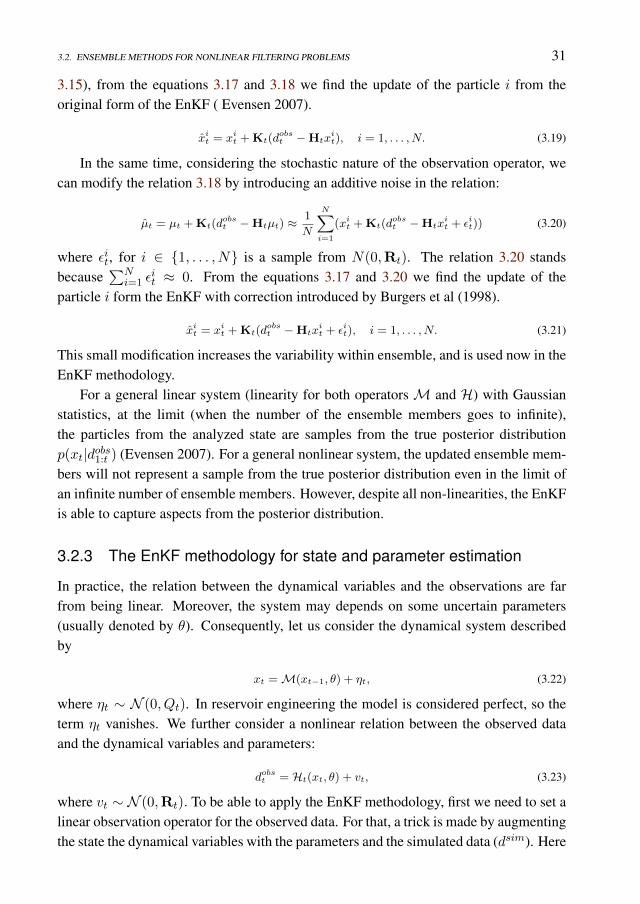
3.2. ENSEMBLE METHODS FOR NONLINEAR FILTERING PROBLEMS 31
3.15), from the equations 3.17 and 3.18 we find the update of the particle i from theoriginal form of the EnKF ( Evensen 2007).
xit = xit + Kt(dobst −Htx
it), i = 1, . . . , N. (3.19)
In the same time, considering the stochastic nature of the observation operator, wecan modify the relation 3.18 by introducing an additive noise in the relation:
µt = µt + Kt(dobst −Htµt) ≈
1
N
N∑i=1
(xit + Kt(dobst −Htx
it + εit)) (3.20)
where εit, for i ∈ 1, . . . , N is a sample from N(0,Rt). The relation 3.20 standsbecause
∑Ni=1 ε
it ≈ 0. From the equations 3.17 and 3.20 we find the update of the
particle i form the EnKF with correction introduced by Burgers et al (1998).
xit = xit + Kt(dobst −Htx
it + εit), i = 1, . . . , N. (3.21)
This small modification increases the variability within ensemble, and is used now in theEnKF methodology.
For a general linear system (linearity for both operators M and H) with Gaussianstatistics, at the limit (when the number of the ensemble members goes to infinite),the particles from the analyzed state are samples from the true posterior distributionp(xt|dobs1:t ) (Evensen 2007). For a general nonlinear system, the updated ensemble mem-bers will not represent a sample from the true posterior distribution even in the limit ofan infinite number of ensemble members. However, despite all non-linearities, the EnKFis able to capture aspects from the posterior distribution.
3.2.3 The EnKF methodology for state and parameter estimation
In practice, the relation between the dynamical variables and the observations are farfrom being linear. Moreover, the system may depends on some uncertain parameters(usually denoted by θ). Consequently, let us consider the dynamical system describedby
xt =M(xt−1, θ) + ηt, (3.22)
where ηt ∼ N (0, Qt). In reservoir engineering the model is considered perfect, so theterm ηt vanishes. We further consider a nonlinear relation between the observed dataand the dynamical variables and parameters:
dobst = Ht(xt, θ) + vt, (3.23)
where vt ∼ N (0,Rt). To be able to apply the EnKF methodology, first we need to set alinear observation operator for the observed data. For that, a trick is made by augmentingthe state the dynamical variables with the parameters and the simulated data (dsim). Here
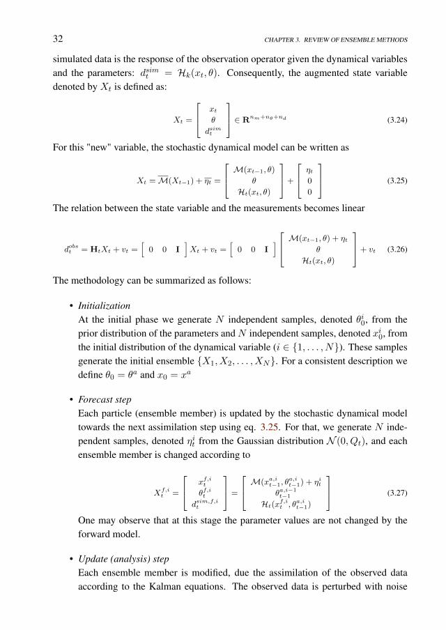
32 CHAPTER 3. REVIEW OF ENSEMBLE METHODS
simulated data is the response of the observation operator given the dynamical variablesand the parameters: dsimt = Hk(xt, θ). Consequently, the augmented state variabledenoted by Xt is defined as:
Xt =
xtθ
dsimt
∈ Rnm+nθ+nd (3.24)
For this "new" variable, the stochastic dynamical model can be written as
Xt =M(Xt−1) + ηt =
M(xt−1, θ)
θ
Ht(xt, θ)
+
ηt0
0
(3.25)
The relation between the state variable and the measurements becomes linear
dobst = HtXt + vt =[
0 0 I]Xt + vt =
[0 0 I
] M(xt−1, θ) + ηtθ
Ht(xt, θ)
+ vt (3.26)
The methodology can be summarized as follows:
• InitializationAt the initial phase we generate N independent samples, denoted θi0, from theprior distribution of the parameters and N independent samples, denoted xi0, fromthe initial distribution of the dynamical variable (i ∈ 1, . . . , N). These samplesgenerate the initial ensemble X1, X2, . . . , XN. For a consistent description wedefine θ0 = θa and x0 = xa
• Forecast stepEach particle (ensemble member) is updated by the stochastic dynamical modeltowards the next assimilation step using eq. 3.25. For that, we generate N inde-pendent samples, denoted ηit from the Gaussian distribution N (0, Qt), and eachensemble member is changed according to
Xf,it =
xf,itθf,it
dsim,f,it
=
M(xa,it−1, θa,it−1) + ηit
θa,i−1t−1
Ht(xf,it , θa,it−1)
(3.27)
One may observe that at this stage the parameter values are not changed by theforward model.
• Update (analysis) stepEach ensemble member is modified, due the assimilation of the observed dataaccording to the Kalman equations. The observed data is perturbed with noise
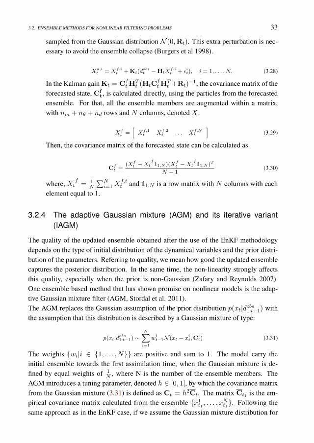
3.2. ENSEMBLE METHODS FOR NONLINEAR FILTERING PROBLEMS 33
sampled from the Gaussian distribution N (0,Rt). This extra perturbation is nec-essary to avoid the ensemble collapse (Burgers et al 1998).
Xa,it = Xf,i
t + Kt(dobst −HtX
f,it + εit), i = 1, . . . , N. (3.28)
In the Kalman gain Kt = CftH
Tt (HtC
ftH
Tt +Rt)
−1, the covariance matrix of theforecasted state, Cf
t, is calculated directly, using the particles from the forecastedensemble. For that, all the ensemble members are augmented within a matrix,with nm + nθ + nd rows and N columns, denoted X:
Xft =
[Xf,1t Xf,2
t . . . Xf,Nt
](3.29)
Then, the covariance matrix of the forecasted state can be calculated as
Cft =
(Xft −Xt
f11,N )(Xf
t −Xtf11,N )T
N − 1(3.30)
where, Xtf
= 1N
∑Ni=1X
f,it and 11,N is a row matrix with N columns with each
element equal to 1.
3.2.4 The adaptive Gaussian mixture (AGM) and its iterative variant(IAGM)
The quality of the updated ensemble obtained after the use of the EnKF methodologydepends on the type of initial distribution of the dynamical variables and the prior distri-bution of the parameters. Referring to quality, we mean how good the updated ensemblecaptures the posterior distribution. In the same time, the non-linearity strongly affectsthis quality, especially when the prior is non-Gaussian (Zafary and Reynolds 2007).One ensemble based method that has shown promise on nonlinear models is the adap-tive Gaussian mixture filter (AGM, Stordal et al. 2011).The AGM replaces the Gaussian assumption of the prior distribution p(xt|dobs1:t−1) withthe assumption that this distribution is described by a Gaussian mixture of type:
p(xt|dobs1:t−1) ∼N∑i=1
wit−1N (xt − xit,Ct) (3.31)
The weights wi|i ∈ 1, . . . , N are positive and sum to 1. The model carry theinitial ensemble towards the first assimilation time, when the Gaussian mixture is de-fined by equal weights of 1
N , where N is the number of the ensemble members. TheAGM introduces a tuning parameter, denoted h ∈ [0, 1], by which the covariance matrixfrom the Gaussian mixture (3.31) is defined as Ct = h2Ct. The matrix Ct1 is the em-pirical covariance matrix calculated from the ensemble x1
t1 , . . . , xNt1. Following the
same approach as in the EnKF case, if we assume the Gaussian mixture distribution for
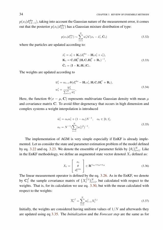
34 CHAPTER 3. REVIEW OF ENSEMBLE METHODS
p(xt|dobs1:t−1), taking into account the Gaussian nature of the measurement error, it comesout that the posterior p(xt|dobs1:t ) has a Gaussian mixture distribution of type:
p(xt|dobs1:t ) ∼N∑i=1
witN (xt − xit, Ct) (3.32)
where the particles are updated according to:
xit = xit + Kt(dobst −Htx
it + εit),
Kt = CtHTt (HtCtH
Tt + Rt)
−1,
Ct = (I−KtHt)Ct.
(3.33)
The weights are updated according to
wit = wt−1Φ(dobst −Htxit,HtCtH
Tt + Rt),
wit =wit∑Ni=1 w
it
,(3.34)
Here, the function Φ(x − µ,C) represents multivariate Gaussian density with mean µand covariance matrix C. To avoid filter degeneracy that occurs in high dimension andcomplex systems a weight interpolation is introduced
wit = αtwit + (1− αt)N−1, αt ∈ [0, 1],
αt = N−1(
N∑i=1
(wit)2)−1.
(3.35)
The implementation of AGM is very simple especially if EnKF is already imple-mented. Let us consider the state and parameter estimation problem of the model definedby eq. 3.22 and eq. 3.23. We denote the ensemble of parameter fields by θiNi=1. Likein the EnKF methodology, we define an augmented state vector denoted Xt defined as:
Xt =
xtθ
dsimt
∈ Rnm+nθ+nd (3.36)
The linear measurement operator is defined by the eq. 3.26. As in the EnKF, we denoteby Cf
t the sample covariance matrix of Xf,it Ni=1, but calculated with respect to the
weights. That is, for its calculation we use eq. 3.30, but with the mean calculated withrespect to the weights:
Xtf
=
N∑i=1
wit−1Xf,it (3.37)
Initially, the weights are considered having uniform values of 1/N and afterwards theyare updated using eq 3.35. The Initialization and the Forecast step are the same as for
3.2. ENSEMBLE METHODS FOR NONLINEAR FILTERING PROBLEMS 35
the EnKF. At each assimilation time, the augmented state vector is updated in the AGM(and IAGM) for each i = 1, . . . , N as
Xa,it = Xf,i
t + CftH
Tt (HtC
ftH
Tt + h−2Rt)
−1(yt −HtX
f,it + εit
), (3.38)
where εit is a sample from the Gaussian measurement error distribution N (0,R). Wenotice that the eq. 3.38 can be written as
Xa,it = Xf,i
t + (h2Cft )HT
t (Ht(h2Cf
t )HTt + Rt)
−1(yt −HtX
f,it + εit
), (3.39)
which is exact the first relation from eq. 3.33. Note that the only difference with a stan-dard EnKF update is the scaling h−2 of the measurement error covariance matrix R. Inother words the linear update is dampened where the dampening factor h ∈ [0, 1] is thebandwidth of the Gaussian mixture (see Stordal et al 2011).
To further improve the AGM on nonlinear models an iterative version, namely theiterative adaptive Gaussian mixture (IAGM) was introduced in Stordal et al 2012. Thenew approach IAGM runs AGM iteratively, with a tuning parameter h ∈ [0, 1]. At theend of an assimilation period, performed with the AGM, an new ensemble is generatedby sampling from the Gaussian mixture defined by the samples at the end of previousiteration (analyzed state). That is, the sampling is performed from
N∑i=1
wij−1N (X −Xa,ij−1, h
2Caj−1) (3.40)
Consequently, the sampling has the form:
Xij = Xi,a
j−1 +h√N − 1
(Xa −Xa11,N )ξi, i = 1, . . . , N. (3.41)
where ξi is multivariate Gaussian with zero mean and covariance matrix IN . To becompletely rigorous, the ratio between the old and new prior for each ensemble membershould then be evaluated, in order to correct the weights assigned to each ensemblemember. However, this would require the estimation of the prior in addition to evaluationof weights in high dimensions. With the weight reduction leading to almost uniformweights due to the dimension, the work is a lot more than the gain. Consequently, weare using uniform weights after resampling. With the new initial ensemble the AGM isthen performed. In most applications only a few iterations, typically two or three, arerequired.
Chapter 4
A probabilistic parametrization forgeological uncertainty estimationusing the Ensemble Kalman Filter(EnKF)
4.1 Introduction
The term facies was introduced in 1837 by the Swiss geologist Amanz Gressly and signi-fies a body of rock with specified characteristics, which formed under certain conditionof sedimentation. The facies types are distinguished either by the petrophysical proper-ties (permeability, porosity, grain size, mineralogy): lithofacies, or by the fossil content:biofacies.The estimation of the (litho)facies distribution into a reservoir domain has two goals;one is related with the high predictive capacity of flow measurements of a reservoirs thatare geologically realistic and the other one is related with the need of accurate propertiesto predict the consequences of changing conditions in the reservoir lifetime (e.g. the re-sponse to enhance recovery). The first step in the assessment of the geologic continuitiesin the subsurface is to define a geological model to simulate plausible facies distributionsthat are consistent with the prior knowledge about subsurface geology (numbers of faciestype that occur, facies proportion, core information, type of patterns etc). The geologi-
This chapter is full reference of the article published in Computational Geosciences, Volume 17, Issue5, pp 813-832, 2013
36
4.1. INTRODUCTION 37
cal model can be constructed using various methods such as an object-based simulationtechnique (Deutsch and Journel 1998, Deutsch and Wang 1996) or a pixel-based simu-lation technique such as Multiple-Point Geostatistique (Guardiano and Srivastava 1993,Strebelle 2002, Caers and Zang 2004). Another approach is the parametrization of thefacies maps with some uncertain variables (parameters), through which we are able toadjust them such that these will honor the underlying knowledge of subsurface geology.These parameters can be calibrated (hence, also the maps) using additional informa-tion about flow measurements within a process named in reservoir engineering, historymatching (HM). A comprehensive description about HM methods is given by Oliver etal. (2008).One of the most promising HM method is the Ensemble Kalman Filter (EnKF) (Evensen1997, 2003, 2006, Aanonsen et al. 2009) which is a Monte Carlo technique introducedin the Kalman filtering framework where the probability density of the state is repre-sented by an ensemble of possible realizations that are simultaneously updated. For theestimation of the spatial distribution of the facies using EnKF as HM method, variousapproaches were proposed, depending on the particularity of geological characterization(number of the occurring facies, type of transition between facies types).Jafarpour and Khodabakhshi (2011) have used for the geological model simulation aMulti-point Geostatistical tool (snesim, Strebelle 2002, 2003) through which the initialensemble is simulated from a training image. Then the EnKF is performed to updatethe log-permeability field and after that, a probability map is constructed for each faciestype, based on a function defined in the log-permeability space that converts the meanlog-permeability field to a probability map. At each assimilation time step a new en-semble is generated, using SNESIM, conditioning the training image to the probabilitymap previously defined. For the case with three facies types, the study uses a trainingimage in which the facies types with lowest and highest permeability do not have directcontact.Lorentzen et al. (2011) proposed for the facies maps simulation a geological simulationmodel based on distances to facies boundaries defined with level set functions (Osherand Fedkiw (2003)). For each facies type a signed distance function is defined as theminimum euclidian distance from each grid cell to boundaries of that facies type. Thesign is positive if the grid cell is in the facies type domain, is negative if the grid cellis outside and is zero if the grid is on the boundary of that facies type. After the EnKFupdate of the distances, the values obtained are no longer distances. An extra procedureis performed in order to transform these updated values to distances and, after that, theupdated facies maps are constructed based on a maximization criterion applied to thetransformed values.Another application of the level set method applied for geometry with 3 facies is pre-sented in the work of Chang et al. (2010), but here, the values of the level set functions
38 CHAPTER 4. PROBABILISTIC PARAMETRIZATION
in some predefined nodes are treated as random variables with known distribution andupdated in the EnKF process. Then, using a interpolation procedure the level set func-tion values are calculated in every grid cell. For the case with 3 facies types, two levelset functions are used and the facies maps are constructed based on sign combination ofthose function values.In our study, for the simulation of the facies maps we use a truncation plurigaussianmethod. This method was introduced by Galli et al. (1994) and further developed by LeLoc’h (1994) and Le Loc’h and Galli (1997). This method is a projection from a contin-uous space (the space determined by the Gaussian random fields (GRF)) into a discretespace (the facies maps space) through a map designed in the GRF space and defined byintersection of some thresholds (values for one GRF, curves for two GRF, surfaces forthree GRF, etc.). In the paper of Le Loc’h et al. (1994), two Gaussian random fieldswere truncated using a rectangular map. They showed various resulting maps changingthe geostatistical characteristics of the GRF (variogram type, isotropy, anisotropy, rangecorrelation, principal direction, etc).Xu et al (2006) propose a "flexible true plurigaussian code for facies simulation", intro-ducing a binary dynamic contact relation matrix (DCM), with which the authors definethe contact relations among facies types. For a bi-dimensional GRF space (bi-Gaussiantruncation) they have used rectangular truncation maps with different number of faciestypes occurring. For three-Gaussian truncation scheme, the maps were constructed basedon intersection of some orthogonal planes defined by the partition of each Gaussian field.In the truncation plurigaussian context, Liu and Oliver (2005) have used for the faciessimulation model a truncation map (in a bi-Gaussian space), constructed using threelines, whose intersections separate the space in seven regions, each having a facies typeassigned. In order to adjust the facies boundaries to the correct position they introducedthe simulation model into a HM process using two methods. One method is a gradient-based method (with some transformations of the map for consistent computation of thesensitivities) and the other is the EnKF. The parameters that define the truncation linescould not by estimated in the HM process and the threshold lines were calibrated in antrial-error procedure. Also, the authors showed, in a 2005 article, that, for the faciesestimations, the EnKF produce better results than the gradient-based method.Agbalaka and Oliver (2008) have used the same simulation model, to generate faciesmaps for a 3D reservoir having three horizontal layers, vertically uncorrelated. They in-troduced the geological model in the EnKF process, together with a localization scheme,defined with the fifth-order compact function of Gaspari and Cohn (1999). The authorsused an internal loop in the EnKF process in order to reposition each facies map of theensemble to the correct facies type in the measurement locations. The reason for doingthat is related to the fact that, after the assimilation of the production data, some of thesimulated facies maps do not preserve the facies observations at the well locations. This
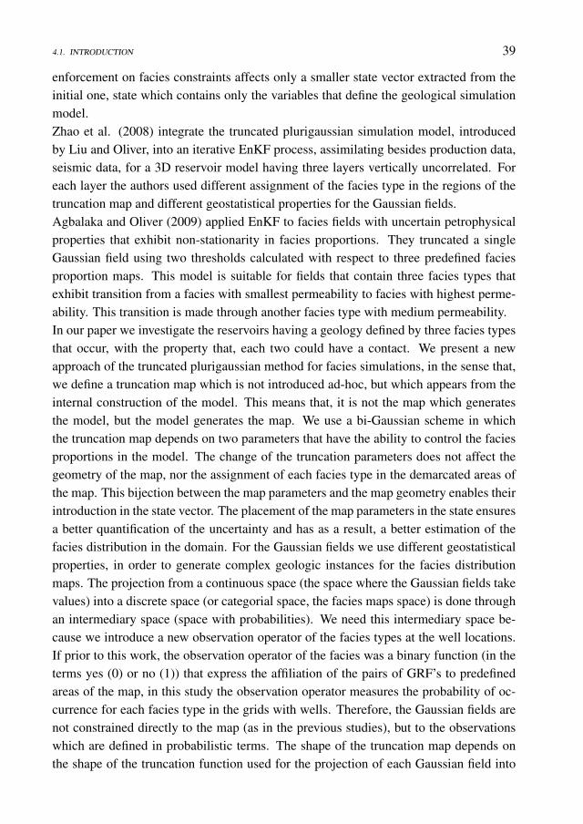
4.1. INTRODUCTION 39
enforcement on facies constraints affects only a smaller state vector extracted from theinitial one, state which contains only the variables that define the geological simulationmodel.Zhao et al. (2008) integrate the truncated plurigaussian simulation model, introducedby Liu and Oliver, into an iterative EnKF process, assimilating besides production data,seismic data, for a 3D reservoir model having three layers vertically uncorrelated. Foreach layer the authors used different assignment of the facies type in the regions of thetruncation map and different geostatistical properties for the Gaussian fields.Agbalaka and Oliver (2009) applied EnKF to facies fields with uncertain petrophysicalproperties that exhibit non-stationarity in facies proportions. They truncated a singleGaussian field using two thresholds calculated with respect to three predefined faciesproportion maps. This model is suitable for fields that contain three facies types thatexhibit transition from a facies with smallest permeability to facies with highest perme-ability. This transition is made through another facies type with medium permeability.In our paper we investigate the reservoirs having a geology defined by three facies typesthat occur, with the property that, each two could have a contact. We present a newapproach of the truncated plurigaussian method for facies simulations, in the sense that,we define a truncation map which is not introduced ad-hoc, but which appears from theinternal construction of the model. This means that, it is not the map which generatesthe model, but the model generates the map. We use a bi-Gaussian scheme in whichthe truncation map depends on two parameters that have the ability to control the faciesproportions in the model. The change of the truncation parameters does not affect thegeometry of the map, nor the assignment of each facies type in the demarcated areas ofthe map. This bijection between the map parameters and the map geometry enables theirintroduction in the state vector. The placement of the map parameters in the state ensuresa better quantification of the uncertainty and has as a result, a better estimation of thefacies distribution in the domain. For the Gaussian fields we use different geostatisticalproperties, in order to generate complex geologic instances for the facies distributionmaps. The projection from a continuous space (the space where the Gaussian fields takevalues) into a discrete space (or categorial space, the facies maps space) is done throughan intermediary space (space with probabilities). We need this intermediary space be-cause we introduce a new observation operator of the facies types at the well locations.If prior to this work, the observation operator of the facies was a binary function (in theterms yes (0) or no (1)) that express the affiliation of the pairs of GRF’s to predefinedareas of the map, in this study the observation operator measures the probability of oc-currence for each facies type in the grids with wells. Therefore, the Gaussian fields arenot constrained directly to the map (as in the previous studies), but to the observationswhich are defined in probabilistic terms. The shape of the truncation map depends onthe shape of the truncation function used for the projection of each Gaussian field into
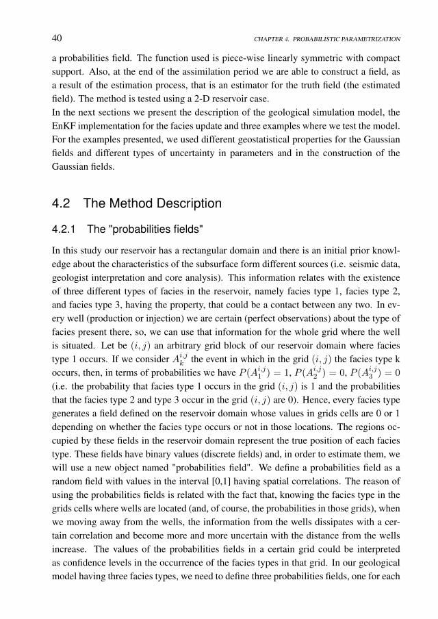
40 CHAPTER 4. PROBABILISTIC PARAMETRIZATION
a probabilities field. The function used is piece-wise linearly symmetric with compactsupport. Also, at the end of the assimilation period we are able to construct a field, asa result of the estimation process, that is an estimator for the truth field (the estimatedfield). The method is tested using a 2-D reservoir case.In the next sections we present the description of the geological simulation model, theEnKF implementation for the facies update and three examples where we test the model.For the examples presented, we used different geostatistical properties for the Gaussianfields and different types of uncertainty in parameters and in the construction of theGaussian fields.
4.2 The Method Description
4.2.1 The "probabilities fields"
In this study our reservoir has a rectangular domain and there is an initial prior knowl-edge about the characteristics of the subsurface form different sources (i.e. seismic data,geologist interpretation and core analysis). This information relates with the existenceof three different types of facies in the reservoir, namely facies type 1, facies type 2,and facies type 3, having the property, that could be a contact between any two. In ev-ery well (production or injection) we are certain (perfect observations) about the type offacies present there, so, we can use that information for the whole grid where the wellis situated. Let be (i, j) an arbitrary grid block of our reservoir domain where faciestype 1 occurs. If we consider Ai,jk the event in which in the grid (i, j) the facies type koccurs, then, in terms of probabilities we have P (Ai,j1 ) = 1, P (Ai,j2 ) = 0, P (Ai,j3 ) = 0
(i.e. the probability that facies type 1 occurs in the grid (i, j) is 1 and the probabilitiesthat the facies type 2 and type 3 occur in the grid (i, j) are 0). Hence, every facies typegenerates a field defined on the reservoir domain whose values in grids cells are 0 or 1depending on whether the facies type occurs or not in those locations. The regions oc-cupied by these fields in the reservoir domain represent the true position of each faciestype. These fields have binary values (discrete fields) and, in order to estimate them, wewill use a new object named "probabilities field". We define a probabilities field as arandom field with values in the interval [0,1] having spatial correlations. The reason ofusing the probabilities fields is related with the fact that, knowing the facies type in thegrids cells where wells are located (and, of course, the probabilities in those grids), whenwe moving away from the wells, the information from the wells dissipates with a cer-tain correlation and become more and more uncertain with the distance from the wellsincrease. The values of the probabilities fields in a certain grid could be interpretedas confidence levels in the occurrence of the facies types in that grid. In our geologicalmodel having three facies types, we need to define three probabilities fields, one for each
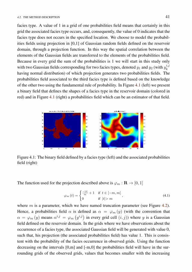
4.2. THE METHOD DESCRIPTION 41
facies type. A value of 1 in a grid of one probabilities field means that certainly in thisgrid the associated facies type occurs, and, consequently, the value of 0 indicates that thefacies type does not occurs in the specified location. We choose to model the probabil-ities fields using projection in [0,1] of Gaussian random fields defined on the reservoirdomain, through a projection function. In this way the spatial correlation between theelements of the Gaussian fields are transferred to the elements of the probabilities field.Because in every grid the sum of the probabilities is 1 we will start in this study onlywith two Gaussian fields corresponding for two facies types, denoted y1 and y2 (with yi,jkhaving normal distribution) of which projection generates two probabilities fields. Theprobabilities field associated to the third facies type is defined based on the knowledgeof the other two using the fundamental rule of probability. In Figure 4.1 (left) we presenta binary field that defines the shapes of a facies type in the reservoir domain (colored inred) and in Figure 4.1 (right) a probabilities field which can be an estimator of that field.
Figure 4.1: The binary field defined by a facies type (left) and the associated probabilitiesfield (right)
The function used for the projection described above is ϕm : R→ [0, 1]
ϕm (t) =
−|t|m
+ 1 if t ∈ [−m,m]
0 if |t|> m, (4.1)
where m is a parameter, which we have named truncation parameter (see Figure 4.2).Hence, a probabilities field α is defined as α = ϕm (y) (with the convention thatα = ϕm (y) means αi,j = ϕm
(yi,j)
in every grid cell (i, j)) where y is a Gaussianfield defined on the reservoir domain. In the grids where we have observations about theoccurrence of a facies type, the associated Gaussian field will be generated with value 0,such that, his projection (the associated probabilities field) has value 1. This is consis-tent with the probability of the facies occurrence in observed grids. Using the functiondecreasing on the intervals [0,m] and [-m,0] the probabilities field will have in the sur-rounding grids of the observed grids, values that becomes smaller with the increasing
42 CHAPTER 4. PROBABILISTIC PARAMETRIZATION
Figure 4.2: The projection function
distance to the observed grid. In addition, the function piece-wise monotony ensures thetransfer of the correlation from the Gaussian fields to the probabilities fields. Knowingthat, in some areas of the reservoir, a certain facies type does not occurs, we have useda threshold value, denoted m, over which the absolute values of the associated Gaussianfield should pass, so that the associated probabilities field to have value 0.
4.2.2 Geological simulation model (Assigning the facies on the grid)
We start with two GRF’s y1 and y2 defined on the entire reservoir domain and α1 andα2 the associated probabilities fields, corresponding to the facies types 1 and 2, whereαk = ϕmk (yk)k=1,2. The parameter mk represent the truncation parameter for therandom field yk. In order to appoint the probabilities field for the third facies we can usethe following rule in each grid cell:
αi,j3 =
1−
(αi,j1 + αi,j2
)if 0 ≤ αi,j1 + αi,j2 ≤ 1
0 if αi,j1 + αi,j2 > 1
(4.2)
Thus, we have defined three probabilities fields corresponding to each facies type. At acertain location (i, j) we assign facies of type k ∈ 1, 2, 3 if
αi,jk = maxαi,jl , l = 1, 3, (4.3)
with the convention that if αi,j1 = αi,j2 ≥ αi,j3 we assign facies type 1 and if αi,j2 =
αi,j3 > αi,j1 we assign facies type 2. The assignment of a facies type to a grid cellsis for the facies type with the highest confidence level of occurrence in that grid. Thismaximization criterion has the role to draw in each probabilities field the location ofthe associated facies type, working for each probabilities field as a threshold. Also, it
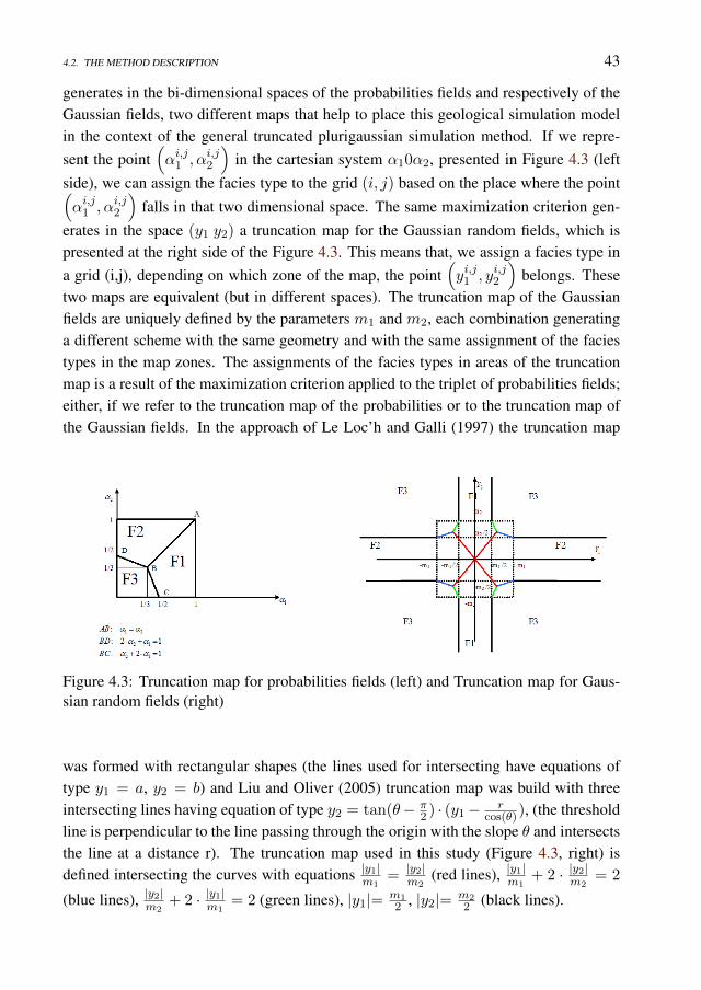
4.2. THE METHOD DESCRIPTION 43
generates in the bi-dimensional spaces of the probabilities fields and respectively of theGaussian fields, two different maps that help to place this geological simulation modelin the context of the general truncated plurigaussian simulation method. If we repre-sent the point
(αi,j1 , αi,j2
)in the cartesian system α10α2, presented in Figure 4.3 (left
side), we can assign the facies type to the grid (i, j) based on the place where the point(αi,j1 , αi,j2
)falls in that two dimensional space. The same maximization criterion gen-
erates in the space (y1 y2) a truncation map for the Gaussian random fields, which ispresented at the right side of the Figure 4.3. This means that, we assign a facies type ina grid (i,j), depending on which zone of the map, the point
(yi,j1 , yi,j2
)belongs. These
two maps are equivalent (but in different spaces). The truncation map of the Gaussianfields are uniquely defined by the parameters m1 and m2, each combination generatinga different scheme with the same geometry and with the same assignment of the faciestypes in the map zones. The assignments of the facies types in areas of the truncationmap is a result of the maximization criterion applied to the triplet of probabilities fields;either, if we refer to the truncation map of the probabilities or to the truncation map ofthe Gaussian fields. In the approach of Le Loc’h and Galli (1997) the truncation map
Figure 4.3: Truncation map for probabilities fields (left) and Truncation map for Gaus-sian random fields (right)
was formed with rectangular shapes (the lines used for intersecting have equations oftype y1 = a, y2 = b) and Liu and Oliver (2005) truncation map was build with threeintersecting lines having equation of type y2 = tan(θ− π
2 ) · (y1− rcos(θ)), (the threshold
line is perpendicular to the line passing through the origin with the slope θ and intersectsthe line at a distance r). The truncation map used in this study (Figure 4.3, right) isdefined intersecting the curves with equations |y1|m1
= |y2|m2
(red lines), |y1|m1+ 2 · |y2|m2
= 2
(blue lines), |y2|m2+ 2 · |y1|m1
= 2 (green lines), |y1|= m12 , |y2|= m2
2 (black lines).
44 CHAPTER 4. PROBABILISTIC PARAMETRIZATION
4.2.3 Truncation parameters
One of the challenges in the truncated plurigaussian method is the choice of the trunca-tion map. In this study the truncation map is uniquely defined by two parameters (namedtruncation parameters). These parameters that initial occur in the definition of the pro-jection function, have an important role in the simulation process due to their propertyto control the facies proportions. In the appendix of this chapter we emphasise the re-lation between the truncation parameters and the expected facies proportions. Also, thetruncation parameters are variable that introduce uncertainty in the model, together withthe geostatistical parameters of the Gaussian fields (the isotropy/anisotropy, the rangecorrelations) and the Gaussian fields themselves. In order to quantify the influence ofthe truncation parameters in the estimation process, in one of the cases, we will intro-duce these parameters in the state vector and perform a comparison with the experimentwhere, we consider that the uncertainty in the model is introduced only by the Gaussianfields.
4.3 Ensemble Kalman filter implementation for facies up-date
In this section, we present the customized implementation of the EnKF in related withour case study.
4.3.1 State vector
The state vector for the jth ensemble member at the kth assimilation step is:
xkj =[yT1 y
T2 m
T1 m
T2 dTsim
]Tj, (4.4)
where y1and y2 represents the two Gaussian random fields, m1, m2 are the truncationparameters of the random fields, and dsim are the simulated observations. The latterones are a combination of simulated production data (oil and water rates, bottom holepressure) and simulated facies observations fsim = [αw1 αw2 ]. So, the state vector fromequation 4.4 becomes:
xkj =[yT1 y
T2 m
T1 m
T2 BHPT qTw qTo α
w,T1 αw,T2
]Tj
(4.5)
In this study, the EnKF is performed without dynamical variables in state vector. There-fore, after each assimilation time, we have chosen to rerun the simulator from time zero,even though this technique will increase the computational cost. For the small models
4.3. ENSEMBLE KALMAN FILTER IMPLEMENTATION FOR FACIES UPDATE 45
of the examples presented, this procedure is not a time consuming, but, for large scalemodels, the computational cost should be considered.
4.3.2 Measurements
The measurements available for the HM process are the observed production data andfacies data at the well locations. Contrary to the numerical character of the productiondata, the facies observations are of categorial type. Therefore, to be able to handle themin the numerical scheme of the history matching algorithm, we need to associate themwith numerical values. When at a certain grid we know that a facies type occurs then theprobability of occurrence of this facies type is one and probability of occurrence of theother two types of facies is zero. Therefore we might use the following assumptions: Ifat the well location we observe
• facies 1 then αi,j1 = 1
αi,j2 = 0
• facies 2 then αi,j1 = 0
αi,j2 = 1
• facies 3 then αi,j1 = 0
αi,j2 = 0
4.3.3 The EnKF implementation
1. Initialization
The uncertainty in the initial ensemble is given by the choice of the two Gaus-sian random fields and by the choice of the truncation parameters (if we includethe truncation parameters in the state vector). Initially, we generate an ensembleof pairs of Gaussian fields y1 and y2 with sequential Gaussian simulation method,specifying the geostatistical properties (isotropy or anisotropy, principal directionsand the range correlation). Throughout this study the number of the ensemblemembers set to 120. The Gaussian fields are generated with constraints given bythe types of facies found in the grids where the wells are situated. If, in a gridwith a well located, we have observation about the existence of facies type 1, thenthe value in this grid for y1 is 0 (y1 is generated with value 0 in this grid suchthat the probability of occurrence is 1) and, of course, if we have observation
46 CHAPTER 4. PROBABILISTIC PARAMETRIZATION
about the existence of facies type 2, then we generate y2 with value 0 in this grid.The truncation parameters are generated with normal distribution and with a meandetermined such that we keep accounted for prior knowledge about facies propor-tions. After the generation of the random Gaussian fields ensemble we performan iterative process to constrain the GRF pairs to the other facies observations (y1
to observations of the facies type 2 and type 3 and y2 to observation of the faciestype 1 and type 3). This iterative process is made with the EnKF method, definingthe state vector
x =[yT1 yT2 αT1 α
T1
]T(4.6)
and the measurement are facies observations at grids where wells are situated.This iterative process stops when α1 and α2 in the grid with observation of faciestype 3 have reached the values such that α1 +α2 < 0.1 (resulting that α3 > 0.9 inthat grid), α1 in grid with observation of facies 2 has property α1 < 0.05 (α3 = 0
there, by definition) and α2 in the grid with observation of facies 1 has propertyα2 < 0.05 (as well α3 = 0 there, by definition). The stopping criterion is chosenin this way because, using two Gaussian fields to model three probabilities fields,we need to ensure similar initial conditions for all facies types. Although, thefacies observations are perfect observations (0 variance) we use the value 0.01 forstandard deviations of facies observations measurement error. We do that, becausewe need that the term
(H Cx H
> + Cobs)−1, from the expression of Kalman gain
to exist, and, the valueCobs = 0.0001·I to not have great importance in the inverse(Agbalaka and Oliver 2008). However, it is possible that, for some initial y1 andy2, the iterative EnKF procedure described above to not lead to an initial ensemblewith the prescribed constraints and actually the iterative process get stuck (eitherthe value of α1 + α2 does not descend below 0.1 or αi for i = 1, 2 does notdescent below 0.05) and is not able to stop. Then, we try the procedure with othertwo random fields, until we find the initial ensemble with correct (prescribed)constraints of the facies observations. As a measure of the spread of the Gaussianfields, we calculate, for both fields, the mean variance and we will watch theirevolutions in the history matching process.
σ2y =
1
ng (ne − 1)
ne∑j=1
ng∑i=1
(yji − yi
)2(4.7)
where ng is the number of the grids, ne is the number of the ensemble membersand yi is the mean value of the random field y in the grid i
yi =1
ne
ne∑j=1
yji (4.8)
4.3. ENSEMBLE KALMAN FILTER IMPLEMENTATION FOR FACIES UPDATE 47
The mean variance is an important indicator because the quality of the forecasterror covariance matrix is directly connected to spreading of the random fields(Agbalaka and Oliver 2008). Also, the mean variance of the Gaussian fields is ameasure of the variability existing in the ensemble at a certain moment. If one ofthe mean variances is very close to zero then, we can state that the ensemble hascollapsed. It is well known that the ensemble collapse is one of the main issueof the EnKF, and, in order to overcome that, we might use either a localizationscheme, or an inflation of the forecast covariance matrix. This is not the case here,where, at the end of the assimilation period, the mean variance of each Gaussianfield is greater than 0.08, value that from our experience ensures enough variabil-ity in the final updated ensemble.
2. Forecast step/Model update
The forecasted state vector at time k + 1:
xk+1,fj =
[yk+1,T1 yk+1,T
2 mk+1,T1 mk+1,T
2 BHPk+1,Tqk+1,Tw qk+1,T
o (αw1 )k+1,T (αw2 )k+1,T]T,fj
,
(4.9)
where y1y2m1
m2
k+1,f
j
=
y1y2m1
m2
k,a
j
(4.10)
[p
s
]k+1,f
j
= M
[ p
s
]k0
,
[y1y2
]k,aj
(4.11)
BHP
qwqo
k+1,f
j
= gpred
[ p
s
]k+1,f
j
,
[y1y2
]k+1,f
j
(4.12)
[αw1αw2
]k+1,f
j
=
[αw2αw2
]k,aj
, (4.13)
where gpred is the prediction operator for the production data. Hence, there areno changes from time k to k + 1 for the values of the Gaussian random fields(eq. 4.10). But, their values have an impact in the changes of the pressures andsaturations at time k + 1 which generates changes in the forecast in productiondata (eq. 4.12). The Gaussian random fields are changed in the update step of theEnKF when the production data is assimilated.
48 CHAPTER 4. PROBABILISTIC PARAMETRIZATION
3. Update step/Measurement update
During the assimilation of production data the updated state vector is calculatedas follows:
xk+1,aj = xk+1,f
j + Cf
xk+1H>k+1
(Hk+1Cf
xk+1H>k+1 + Cprod
obs,k+1
)−1
[dprodobsj ,k+1
−Hk+1xk+1,fj
], (4.14)
where H represents observation operator for the production data, Cprod
obs representsthe error covariance matrix for the production data, Cxf represents the forecastederror covariance of the ensemble, and dprodobsj
are the observed production data. Inorder assimilate the facies data we separate part of the state vector as in:
xk+1j =
[yT1 y
T2 m
T1 m
T2 α
w,T1 αw,T2
]T,k+1
j, (4.15)
If, after the assimilation of the facies data, some of the ensemble members violatethe position of the facies type 3 in the grids where we have observations about theirexistence, we perform an iterative enforcement on facies observations (because therandom fields y1 and y2 are generated with value 0 in grids where facies type 1and type 2 respectively occur, during the HM process the position of the faciestype 1 and type 2 are not violated). The iterative process will stop when the valueof α3 in the grids where we have observation about existence of the facies type 3is greater than α1 and α2 in those grids. In the iterative process explained abovethe uncertainty for the facies observations is represented by the error covariancematrix of 0.0001I.
4. The estimated field
One of the targets of this study is to find a field of facies distribution which isan estimator for the "truth" field (or reference field). In the previous studies usingtruncated plurigaussian method for facies simulations, an estimator of the truthfield could not be directly presented, because the posterior mean of the randomfields could not generate a plausible geological model. In this study, for eachfacies type, we calculate the mean of probabilities fields (named estimated prob-abilities field), that will be an estimator of the associated binary field (generatedby the facies type). Using these three estimated probabilities fields we define theestimated field with the maximization criterion, meaning that the assignment of afacies type in a grid is made for the facies type with the highest value of probabil-

4.3. ENSEMBLE KALMAN FILTER IMPLEMENTATION FOR FACIES UPDATE 49
ity in that grid. For k = 1 or k = 2 we have first two estimated probabilities fieldsas
αi,jk =1
ne
ne∑l=1
ϕmk,l
(yi,jk,l
)(4.16)
For the mean of the probability of occurrence of the facies type 3 we use therelation
αi,j3 =
1−
(αi,j1 + αi,j2
)if 0 ≤ αi,j1 + αi,j2 ≤ 1
0 if αi,j1 + αi,j2 > 1
(4.17)
Consequently, in the estimated field we assign the facies type k in the grid (i, i) if
αi,jk = maxαi,jl , l = 1, 3, (4.18)
Also, we will use the same rule as in the main procedure, regarding the cases whenthe probabilities are equals in the grids.
4.3.4 Indicators for the quality of the estimations
The first comparison between updated fields and reference field or between different esti-mated fields of the same reference field is made by visualizing the facies maps. But thisvisualization is not sufficient, therefore, we define some quantitative indicators whichcan show the quality of the estimation.(1) Root Mean Square Error (RMS) calculated for permeability:
RMS(k) =
√√√√ 1
ng
ng∑i=1
(krefi − kesti)2 (4.19)
where ng is the number of grid blocks krefi and kesti represent the values of perme-ability for reference field and estimated field for grid block i.(2) Percentage of grid fit between the estimated field and the reference field:
Percentage =1
ng
ng∑i=1
mi × 100 (4.20)
where mi = 1 if in the grid i the estimated field and the reference field has the samefacies type and mi = 0 if we have a misfit between the facies type existing in estimatedfield and facies type existing in reference field.(3) Root Mean Square Error (RMS) of the Water Rates (WR) prediction for the next 100days (10 time steps), calculated for the estimated field and for the mean of the updatedensemble members and, respectively for Total Rates Production (TR) of the estimated
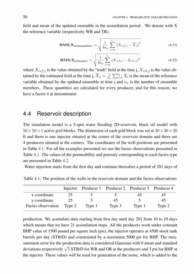
50 CHAPTER 4. PROBABILISTIC PARAMETRIZATION
field and mean of the updated ensemble in the assimilation period . We denote with Xthe reference variable (respectively WR and TR).
RMS(Xmeanupdate) =
√√√√ 1
4ng
t1∑j=t0
(Xref,j −Xj
)2(4.21)
RMS(Xestimate) =
√√√√ 1
4ng
t1∑j=t0
(Xref,j −Xest,j)2 (4.22)
whereXref,j is the value obtained by the "truth" field at the time j,Xest,j is the value ob-tained by the estimated field at the time j,Xj = 1
ne
∑nei=1Xi is the mean of the reference
variable obtained by the updated ensemble at time j and ne is the number of ensemblemembers. These quantities are calculated for every producer, and for this reason, wehave a factor 4 at denominator.
4.4 Reservoir description
The simulation model is a 5-spot water flooding 2D-reservoir, black oil model with50×50×1 active grid blocks. The dimension of each grid block was set at 30×30×20
ft and there is one injector situated at the center of the reservoir domain and there are4 producers situated at the corners. The coordinates of the well positions are presentedin Table 4.1. For all the examples presented we use the facies observations presented inTable 4.1. The values of the permeability and porosity corresponding to each facies typeare presented in Table 4.2.Water injection starts from the first day and continue thereafter a period of 201 days of
Table 4.1: The position of the wells in the reservoir domain and the facies observations
Injector Producer 1 Producer 2 Producer 3 Producer 4x coordinate 25 5 5 45 45y coordinate 25 5 45 5 45
Facies observation Type 2 Type 1 Type 3 Type 1 Type 2
production. We assimilate data starting from first day until day 201 from 10 to 10 dayswhich means that we have 21 assimilation steps. All the producers work under constantBHP value of 1500 pound per square inch (psi), the injector operates at 4500 stock tankbarrels per day (STB/D) and constrained by a maximum 5000 psi for BHP. The mea-surement error for the production data is considered Gaussian with 0 mean and standarddeviations respectively
√5 STB/D for WR and OR at the producers and 3 psi for BHP at
the injector. These values will be used for generation of the noise, which is added to the
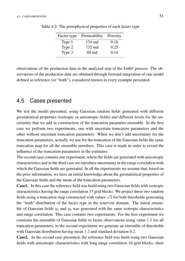
4.5. CASES PRESENTED 51
Table 4.2: The petrophysical properties of each facies type
Facies type Permeability PorosityType 1 174 md 0.18Type 2 732 md 0.25Type 3 80 md 0.14
observations of the production data in the analyzed step of the EnKF process. The ob-servations of the production data are obtained through forward integration of one modeldefined as reference (or "truth"), considered known in every example presented.
4.5 Cases presented
We test the model presented, using Gaussian random fields generated with differentgeostatistical properties (isotropic or anisotropic fields) and different levels for the un-certainty that we add in construction of the truncation parameter ensemble. In the firstcase we perform two experiments, one with uncertain truncation parameters and theother without uncertain truncation parameters. When we don’t add uncertainty for thetruncation parameters, actually we use for the truncation of the Gaussian fields the sametruncation map for all the ensemble members. This case is made in order to reveal theinfluence of the truncation parameters in the estimates.The second case contains one experiment, where the fields are generated with anisotropiccharacteristics and in the third case we introduce uncertainty in the range correlation withwhich the Gaussian fields are generated. In all the experiments we assume that, based onthe prior information, we have an initial knowledge about the geostatistical properties ofthe Gaussian fields and the mean of the truncation parameters.Case1. In this case the reference field was build using two Gaussian fields with isotropiccharacteristics having the range correlation 17 grid blocks. We project these two randomfields using a truncation map constructed with values
√2 for both thresholds generating
the "truth" distribution of the facies type in the reservoir domain. The initial ensem-ble of Gaussian fields y1 and y2 was generated with the same isotropic characteristicsand range correlation. This case contains two experiments. For the first experiment weconstrain the ensemble of Gaussian fields to facies observations using value 1.5 for alltruncation parameters, in the second experiment we generate an ensemble of thresholdswith Gaussian distribution having mean 1.5 and standard deviation 0.2.Case2. In the second case presented, the reference field was build using two Gaussianfields with anisotropic characteristics with long range correlation 16 grid blocks, short
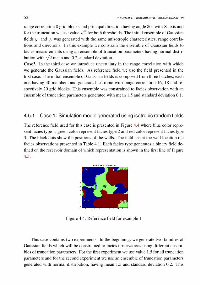
52 CHAPTER 4. PROBABILISTIC PARAMETRIZATION
range correlation 8 grid blocks and principal direction having angle 30 with X-axis andfor the truncation we use value
√2 for both thresholds. The initial ensemble of Gaussian
fields y1 and y2 was generated with the same anisotropic characteristics, range correla-tions and directions. In this example we constrain the ensemble of Gaussian fields tofacies measurements using an ensemble of truncation parameters having normal distri-bution with
√2 mean and 0.2 standard deviation.
Case3. In the third case we introduce uncertainty in the range correlation with whichwe generate the Gaussian fields. As reference field we use the field presented in thefirst case. The initial ensemble of Gaussian fields is composed from three batches, eachone having 40 members and generated isotropic with range correlation 16, 18 and re-spectively 20 grid blocks. This ensemble was constrained to facies observation with anensemble of truncation parameters generated with mean 1.5 and standard deviation 0.1.
4.5.1 Case 1: Simulation model generated using isotropic random fields
The reference field used for this case is presented in Figure 4.4 where blue color repre-sent facies type 1, green color represent facies type 2 and red color represent facies type3. The black dots show the positions of the wells. The field has at the well location thefacies observations presented in Table 4.1. Each facies type generates a binary field de-fined on the reservoir domain of which representation is shown in the first line of Figure4.5.
Figure 4.4: Reference field for example 1
This case contains two experiments. In the beginning, we generate two families ofGaussian fields which will be constrained to facies observations using different ensem-bles of truncation parameters. For the first experiment we use value 1.5 for all truncationparameters and for the second experiment we use an ensemble of truncation parametersgenerated with normal distribution, having mean 1.5 and standard deviation 0.2. This
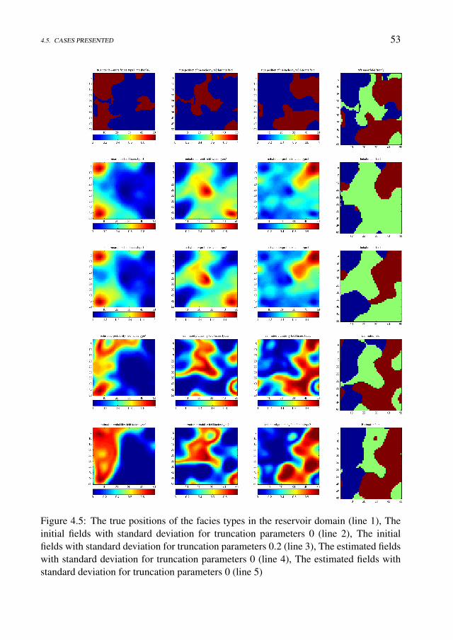
4.5. CASES PRESENTED 53
Figure 4.5: The true positions of the facies types in the reservoir domain (line 1), Theinitial fields with standard deviation for truncation parameters 0 (line 2), The initialfields with standard deviation for truncation parameters 0.2 (line 3), The estimated fieldswith standard deviation for truncation parameters 0 (line 4), The estimated fields withstandard deviation for truncation parameters 0 (line 5)

54 CHAPTER 4. PROBABILISTIC PARAMETRIZATION
means that in the first experiment we do not introduce uncertainty in the truncation pa-rameters. The choice of 1.5 as the mean value for the truncation parameters is madetaking into account the prior knowledge of the facies proportions of the reference field.We obtain two initial ensembles of Gaussian fields that are derived from the same en-semble of GRF which means that these two ensembles contain similar information (aswe see from the initial mean probabilities fields presented in Figures 4.5 (lines 2 and 3)).In Figure 4.5, lines 2 and 3, we presents, for the experiments, the initial fields (whichcontains initial mean fields for the probabilities of occurrence of the facies type and theinitial "mean" field) and in lines 4 and 5 the results obtained after the assisted HM per-forming. The results presented are the estimated probabilities fields for all the faciestypes and the estimated field. From these pictures we can observe that, for the initialprobabilities fields of facies type 1 and type 2 the region with probabilities greater than0 are diffusive distributed in the reservoir domain, whereas in the estimated probabilitiesfields are more clearly shaped. If in the initial fields the shapes are contoured with thevalues near to 0.4 in the estimated fields the shapes are contoured by the values near to0.7. The variability in the initial ensemble of random fields can be observed in the dif-fusive distribution of the shapes of the facies type 1 and type 2 in the initial maps. Also,in the initial mean field (and also in the initial ensemble of facies maps) the facies type3 have the smallest proportion because of two causes; first, only in the well 2 we haveobservation about occurrence of that facies type and second, because of the constructionof the simulated model, where probability of occurrence of the facies type 3 is appointedbased on fundamental rule of probabilities. After the assimilation period, the facies pro-portion in the estimated field is close to the true facies proportions ("truth" field has thefacies proportions 0.36:0.24:0.40 and in the estimated field has the facies proportions0.34:0.24:0.41). With a visual inspection of the estimated fields (Figure 4.5 lines 4 and 5last pictures) we can conclude that these fields are good estimators for the reference fieldbut for a better quantification of the estimation we will compare the indicators presentedpreviously. In Table 4.3 we present the values for the indicators calculated for the esti-mated fields. We can easily observe that indicators of the estimated field resulting fromHM process with uncertainty in the truncation parameters have better values than the in-dicators of the estimated field obtained without uncertainty in the truncation parameters.Knowing that the true facies proportions is 0.36:0.24:0.40, from the Table 4.3 we canobserve that in the both cases the variability of the initial ensemble incorporates this truevalue. However, only the updated ensemble for the case with variability in the truncationparameters preserves this property. We have repeated the experiments for several initialensembles and the conclusion is that, the updated fields of the experiment where wetake into account the uncertainty in the truncation parameters, has a higher percentageof grid fitting and a better quantification of the facies proportions then the other updatedfields. Concerning the RMS calculated for the rates, either for the ensembles, or for the
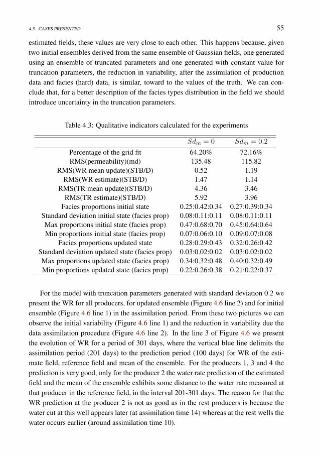
4.5. CASES PRESENTED 55
estimated fields, these values are very close to each other. This happens because, giventwo initial ensembles derived from the same ensemble of Gaussian fields, one generatedusing an ensemble of truncated parameters and one generated with constant value fortruncation parameters, the reduction in variability, after the assimilation of productiondata and facies (hard) data, is similar, toward to the values of the truth. We can con-clude that, for a better description of the facies types distribution in the field we shouldintroduce uncertainty in the truncation parameters.
Table 4.3: Qualitative indicators calculated for the experiments
Sdm = 0 Sdm = 0.2
Percentage of the grid fit 64.20% 72.16%RMS(permeability)(md) 135.48 115.82
RMS(WR mean update)(STB/D) 0.52 1.19RMS(WR estimate)(STB/D) 1.47 1.14
RMS(TR mean update)(STB/D) 4.36 3.46RMS(TR estimate)(STB/D) 5.92 3.96
Facies proportions initial state 0.25:0.42:0.34 0.27:0.39:0.34Standard deviation initial state (facies prop) 0.08:0.11:0.11 0.08:0.11:0.11Max proportions initial state (facies prop) 0.47:0.68:0.70 0.45:0.64:0.64Min proportions initial state (facies prop) 0.07:0.06:0.10 0.09:0.07:0.08
Facies proportions updated state 0.28:0.29:0.43 0.32:0.26:0.42Standard deviation updated state (facies prop) 0.03:0.02:0.02 0.03:0.02:0.02Max proportions updated state (facies prop) 0.34:0.32:0.48 0.40:0.32:0.49Min proportions updated state (facies prop) 0.22:0.26:0.38 0.21:0.22:0.37
For the model with truncation parameters generated with standard deviation 0.2 wepresent the WR for all producers, for updated ensemble (Figure 4.6 line 2) and for initialensemble (Figure 4.6 line 1) in the assimilation period. From these two pictures we canobserve the initial variability (Figure 4.6 line 1) and the reduction in variability due thedata assimilation procedure (Figure 4.6 line 2). In the line 3 of Figure 4.6 we presentthe evolution of WR for a period of 301 days, where the vertical blue line delimits theassimilation period (201 days) to the prediction period (100 days) for WR of the esti-mate field, reference field and mean of the ensemble. For the producers 1, 3 and 4 theprediction is very good, only for the producer 2 the water rate prediction of the estimatedfield and the mean of the ensemble exhibits some distance to the water rate measured atthat producer in the reference field, in the interval 201-301 days. The reason for that theWR prediction at the producer 2 is not as good as in the rest producers is because thewater cut at this well appears later (at assimilation time 14) whereas at the rest wells thewater occurs earlier (around assimilation time 10).
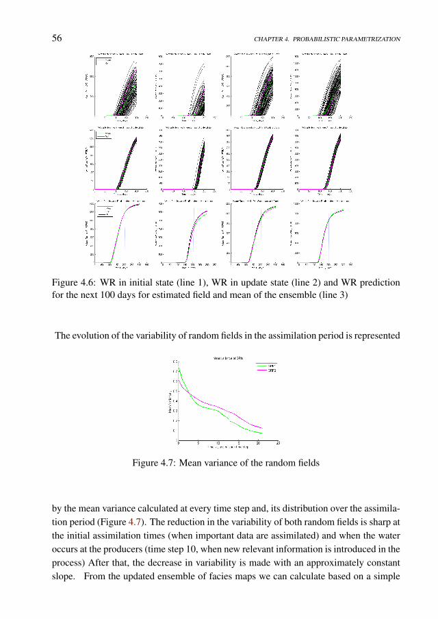
56 CHAPTER 4. PROBABILISTIC PARAMETRIZATION
Figure 4.6: WR in initial state (line 1), WR in update state (line 2) and WR predictionfor the next 100 days for estimated field and mean of the ensemble (line 3)
The evolution of the variability of random fields in the assimilation period is represented
Figure 4.7: Mean variance of the random fields
by the mean variance calculated at every time step and, its distribution over the assimila-tion period (Figure 4.7). The reduction in the variability of both random fields is sharp atthe initial assimilation times (when important data are assimilated) and when the wateroccurs at the producers (time step 10, when new relevant information is introduced in theprocess) After that, the decrease in variability is made with an approximately constantslope. From the updated ensemble of facies maps we can calculate based on a simple
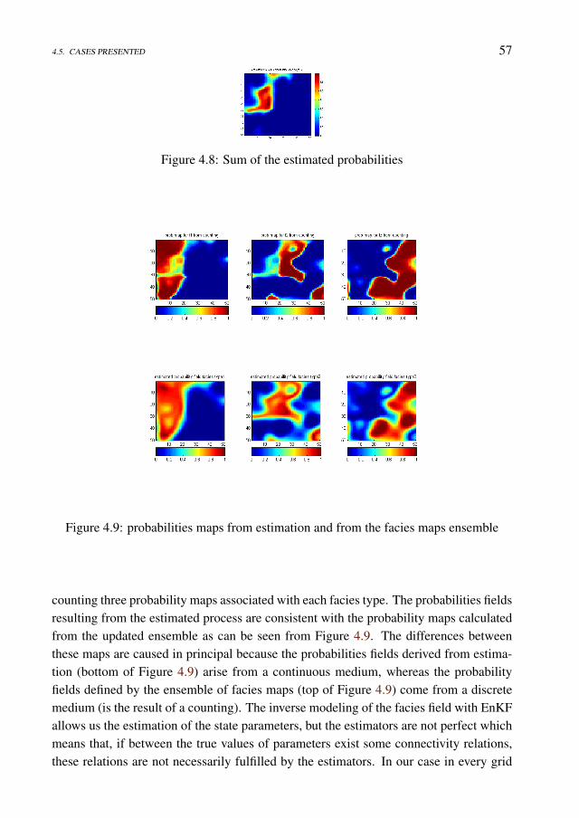
4.5. CASES PRESENTED 57
Figure 4.8: Sum of the estimated probabilities
Figure 4.9: probabilities maps from estimation and from the facies maps ensemble
counting three probability maps associated with each facies type. The probabilities fieldsresulting from the estimated process are consistent with the probability maps calculatedfrom the updated ensemble as can be seen from Figure 4.9. The differences betweenthese maps are caused in principal because the probabilities fields derived from estima-tion (bottom of Figure 4.9) arise from a continuous medium, whereas the probabilityfields defined by the ensemble of facies maps (top of Figure 4.9) come from a discretemedium (is the result of a counting). The inverse modeling of the facies field with EnKFallows us the estimation of the state parameters, but the estimators are not perfect whichmeans that, if between the true values of parameters exist some connectivity relations,these relations are not necessarily fulfilled by the estimators. In our case in every grid
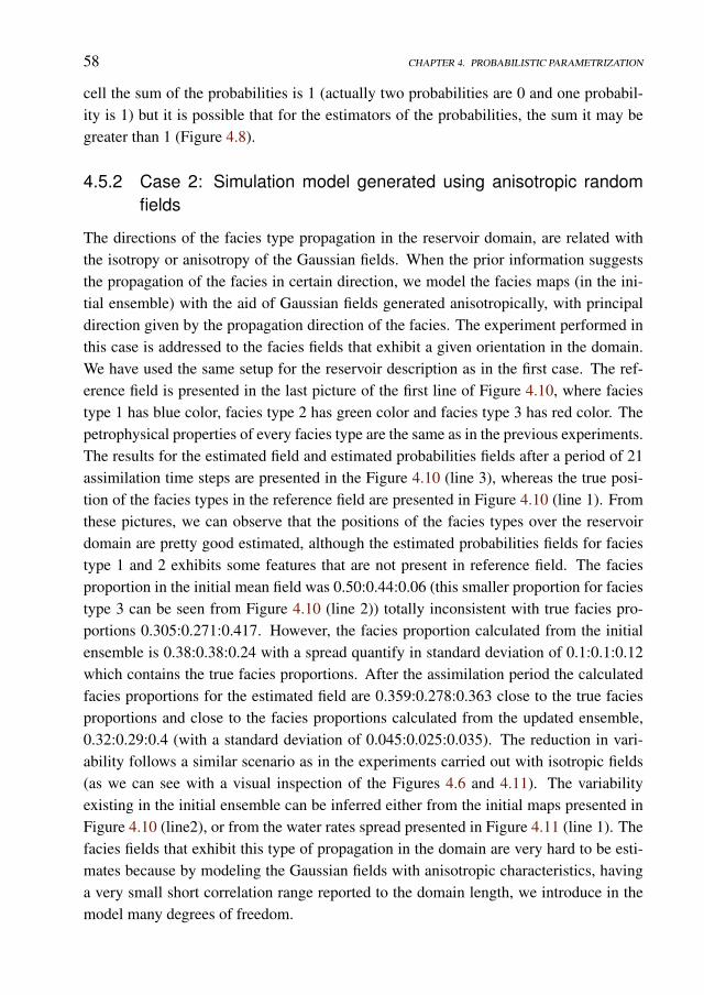
58 CHAPTER 4. PROBABILISTIC PARAMETRIZATION
cell the sum of the probabilities is 1 (actually two probabilities are 0 and one probabil-ity is 1) but it is possible that for the estimators of the probabilities, the sum it may begreater than 1 (Figure 4.8).
4.5.2 Case 2: Simulation model generated using anisotropic randomfields
The directions of the facies type propagation in the reservoir domain, are related withthe isotropy or anisotropy of the Gaussian fields. When the prior information suggeststhe propagation of the facies in certain direction, we model the facies maps (in the ini-tial ensemble) with the aid of Gaussian fields generated anisotropically, with principaldirection given by the propagation direction of the facies. The experiment performed inthis case is addressed to the facies fields that exhibit a given orientation in the domain.We have used the same setup for the reservoir description as in the first case. The ref-erence field is presented in the last picture of the first line of Figure 4.10, where faciestype 1 has blue color, facies type 2 has green color and facies type 3 has red color. Thepetrophysical properties of every facies type are the same as in the previous experiments.The results for the estimated field and estimated probabilities fields after a period of 21assimilation time steps are presented in the Figure 4.10 (line 3), whereas the true posi-tion of the facies types in the reference field are presented in Figure 4.10 (line 1). Fromthese pictures, we can observe that the positions of the facies types over the reservoirdomain are pretty good estimated, although the estimated probabilities fields for faciestype 1 and 2 exhibits some features that are not present in reference field. The faciesproportion in the initial mean field was 0.50:0.44:0.06 (this smaller proportion for faciestype 3 can be seen from Figure 4.10 (line 2)) totally inconsistent with true facies pro-portions 0.305:0.271:0.417. However, the facies proportion calculated from the initialensemble is 0.38:0.38:0.24 with a spread quantify in standard deviation of 0.1:0.1:0.12which contains the true facies proportions. After the assimilation period the calculatedfacies proportions for the estimated field are 0.359:0.278:0.363 close to the true faciesproportions and close to the facies proportions calculated from the updated ensemble,0.32:0.29:0.4 (with a standard deviation of 0.045:0.025:0.035). The reduction in vari-ability follows a similar scenario as in the experiments carried out with isotropic fields(as we can see with a visual inspection of the Figures 4.6 and 4.11). The variabilityexisting in the initial ensemble can be inferred either from the initial maps presented inFigure 4.10 (line2), or from the water rates spread presented in Figure 4.11 (line 1). Thefacies fields that exhibit this type of propagation in the domain are very hard to be esti-mates because by modeling the Gaussian fields with anisotropic characteristics, havinga very small short correlation range reported to the domain length, we introduce in themodel many degrees of freedom.
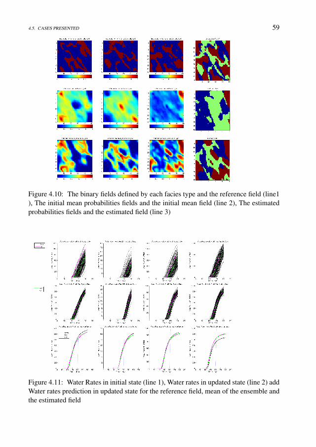
4.5. CASES PRESENTED 59
Figure 4.10: The binary fields defined by each facies type and the reference field (line1), The initial mean probabilities fields and the initial mean field (line 2), The estimatedprobabilities fields and the estimated field (line 3)
Figure 4.11: Water Rates in initial state (line 1), Water rates in updated state (line 2) addWater rates prediction in updated state for the reference field, mean of the ensemble andthe estimated field
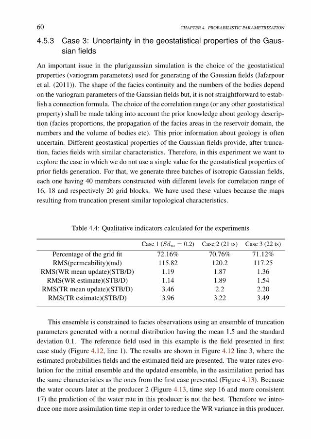
60 CHAPTER 4. PROBABILISTIC PARAMETRIZATION
4.5.3 Case 3: Uncertainty in the geostatistical properties of the Gaus-sian fields
An important issue in the plurigaussian simulation is the choice of the geostatisticalproperties (variogram parameters) used for generating of the Gaussian fields (Jafarpouret al. (2011)). The shape of the facies continuity and the numbers of the bodies dependon the variogram parameters of the Gaussian fields but, it is not straightforward to estab-lish a connection formula. The choice of the correlation range (or any other geostatisticalproperty) shall be made taking into account the prior knowledge about geology descrip-tion (facies proportions, the propagation of the facies areas in the reservoir domain, thenumbers and the volume of bodies etc). This prior information about geology is oftenuncertain. Different geostastical properties of the Gaussian fields provide, after trunca-tion, facies fields with similar characteristics. Therefore, in this experiment we want toexplore the case in which we do not use a single value for the geostatistical properties ofprior fields generation. For that, we generate three batches of isotropic Gaussian fields,each one having 40 members constructed with different levels for correlation range of16, 18 and respectively 20 grid blocks. We have used these values because the mapsresulting from truncation present similar topological characteristics.
Table 4.4: Qualitative indicators calculated for the experiments
Case 1 (Sdm = 0.2) Case 2 (21 ts) Case 3 (22 ts)
Percentage of the grid fit 72.16% 70.76% 71.12%RMS(permeability)(md) 115.82 120.2 117.25
RMS(WR mean update)(STB/D) 1.19 1.87 1.36RMS(WR estimate)(STB/D) 1.14 1.89 1.54
RMS(TR mean update)(STB/D) 3.46 2.2 2.20RMS(TR estimate)(STB/D) 3.96 3.22 3.49
This ensemble is constrained to facies observations using an ensemble of truncationparameters generated with a normal distribution having the mean 1.5 and the standarddeviation 0.1. The reference field used in this example is the field presented in firstcase study (Figure 4.12, line 1). The results are shown in Figure 4.12 line 3, where theestimated probabilities fields and the estimated field are presented. The water rates evo-lution for the initial ensemble and the updated ensemble, in the assimilation period hasthe same characteristics as the ones from the first case presented (Figure 4.13). Becausethe water occurs later at the producer 2 (Figure 4.13, time step 16 and more consistent17) the prediction of the water rate in this producer is not the best. Therefore we intro-duce one more assimilation time step in order to reduce the WR variance in this producer.
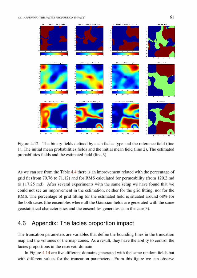
4.6. APPENDIX: THE FACIES PROPORTION IMPACT 61
Figure 4.12: The binary fields defined by each facies type and the reference field (line1), The initial mean probabilities fields and the initial mean field (line 2), The estimatedprobabilities fields and the estimated field (line 3)
As we can see from the Table 4.4 there is an improvement related with the percentage ofgrid fit (from 70.76 to 71.12) and for RMS calculated for permeability (from 120.2 mdto 117.25 md). After several experiments with the same setup we have found that wecould not see an improvement in the estimation, neither for the grid fitting, nor for theRMS. The percentage of grid fitting for the estimated field is situated around 68% forthe both cases (the ensembles where all the Gaussian fields are generated with the samegeostatistical characteristics and the ensembles generates as in the case 3).
4.6 Appendix: The facies proportion impact
The truncation parameters are variables that define the bounding lines in the truncationmap and the volumes of the map zones. As a result, they have the ability to control thefacies proportions in the reservoir domain.
In Figure 4.14 are five different domains generated with the same random fields butwith different values for the truncation parameters. From this figure we can observe
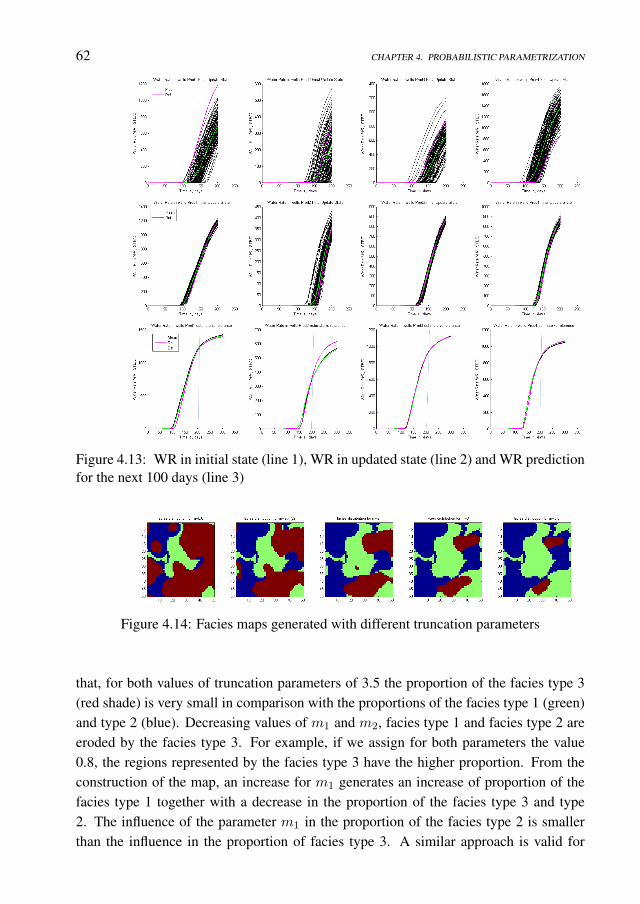
62 CHAPTER 4. PROBABILISTIC PARAMETRIZATION
Figure 4.13: WR in initial state (line 1), WR in updated state (line 2) and WR predictionfor the next 100 days (line 3)
Figure 4.14: Facies maps generated with different truncation parameters
that, for both values of truncation parameters of 3.5 the proportion of the facies type 3(red shade) is very small in comparison with the proportions of the facies type 1 (green)and type 2 (blue). Decreasing values of m1 and m2, facies type 1 and facies type 2 areeroded by the facies type 3. For example, if we assign for both parameters the value0.8, the regions represented by the facies type 3 have the higher proportion. From theconstruction of the map, an increase for m1 generates an increase of proportion of thefacies type 1 together with a decrease in the proportion of the facies type 3 and type2. The influence of the parameter m1 in the proportion of the facies type 2 is smallerthan the influence in the proportion of facies type 3. A similar approach is valid for
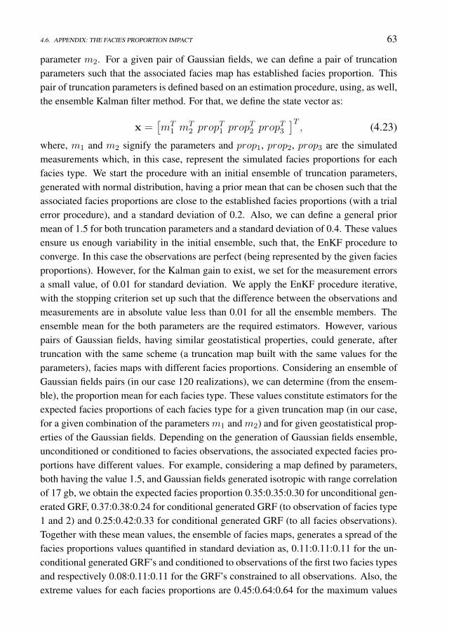
4.6. APPENDIX: THE FACIES PROPORTION IMPACT 63
parameter m2. For a given pair of Gaussian fields, we can define a pair of truncationparameters such that the associated facies map has established facies proportion. Thispair of truncation parameters is defined based on an estimation procedure, using, as well,the ensemble Kalman filter method. For that, we define the state vector as:
x =[mT
1 mT2 prop
T1 prop
T2 prop
T3
]T, (4.23)
where, m1 and m2 signify the parameters and prop1, prop2, prop3 are the simulatedmeasurements which, in this case, represent the simulated facies proportions for eachfacies type. We start the procedure with an initial ensemble of truncation parameters,generated with normal distribution, having a prior mean that can be chosen such that theassociated facies proportions are close to the established facies proportions (with a trialerror procedure), and a standard deviation of 0.2. Also, we can define a general priormean of 1.5 for both truncation parameters and a standard deviation of 0.4. These valuesensure us enough variability in the initial ensemble, such that, the EnKF procedure toconverge. In this case the observations are perfect (being represented by the given faciesproportions). However, for the Kalman gain to exist, we set for the measurement errorsa small value, of 0.01 for standard deviation. We apply the EnKF procedure iterative,with the stopping criterion set up such that the difference between the observations andmeasurements are in absolute value less than 0.01 for all the ensemble members. Theensemble mean for the both parameters are the required estimators. However, variouspairs of Gaussian fields, having similar geostatistical properties, could generate, aftertruncation with the same scheme (a truncation map built with the same values for theparameters), facies maps with different facies proportions. Considering an ensemble ofGaussian fields pairs (in our case 120 realizations), we can determine (from the ensem-ble), the proportion mean for each facies type. These values constitute estimators for theexpected facies proportions of each facies type for a given truncation map (in our case,for a given combination of the parameters m1 and m2) and for given geostatistical prop-erties of the Gaussian fields. Depending on the generation of Gaussian fields ensemble,unconditioned or conditioned to facies observations, the associated expected facies pro-portions have different values. For example, considering a map defined by parameters,both having the value 1.5, and Gaussian fields generated isotropic with range correlationof 17 gb, we obtain the expected facies proportion 0.35:0.35:0.30 for unconditional gen-erated GRF, 0.37:0.38:0.24 for conditional generated GRF (to observation of facies type1 and 2) and 0.25:0.42:0.33 for conditional generated GRF (to all facies observations).Together with these mean values, the ensemble of facies maps, generates a spread of thefacies proportions values quantified in standard deviation as, 0.11:0.11:0.11 for the un-conditional generated GRF’s and conditioned to observations of the first two facies typesand respectively 0.08:0.11:0.11 for the GRF’s constrained to all observations. Also, theextreme values for each facies proportions are 0.45:0.64:0.64 for the maximum values

64 CHAPTER 4. PROBABILISTIC PARAMETRIZATION
and respectively 0.09:0.06:0.08 for the minimum values. In this study we do not use thefacies proportions as measurements, even though we could have some prior knowledgeabout these (together with an uncertainty bandwidth). The choice for the prior values oftruncation parameters is made, such that the spread of the facies proportions (calculatedfrom the ensemble) to contains the expected facies proportions given by the geologist.This means that the choice of the prior values for the truncation parameters (and fromhere for the truncation map) could be made in various ways, as long we have enoughvariability in the initial ensemble which incorporates the prior knowledge.
Chapter 5
An adaptive plurigaussiansimulation (APS) model forgeological uncertaintyquantification using the EnKF
5.1 Introduction
For the implementation of any assisted history matching (AHM) model in the area ofreservoir engineering, one of the most important topics to address is the reservoir geol-ogy. When referring to geological description we have in mind facies distribution, faultsposition or top/base surfaces of the geological layers. Usually the initial knowledgeabout the geology is very uncertain, which is very attractive for stochastic AHM mod-els. In this study we are interested in the facies distribution and try to reduce its initialuncertainty using additional information given by the production data when available.In order to quantify the geological uncertainty, firstly, we have to define the geologicalsimulation model. Using this model, we generate possible facies realizations (distribu-tions) on the reservoir domain. These facies instances must be consistent with the priorknowledge about the reservoir geology (the number of the facies types, the possible tran-sition between facies types, the direction of the facies, the geometry of the facies, etc.).Secondly, for the estimation purposes and for uncertainty propagation and hence, quan-tification, we use as history matching (HM) method the ensemble Kalman filter (EnKF).
This chapter is full reference of an article submitted to Computational Geosciences
65
66 CHAPTER 5. THE ADAPTIVE PLURIGAUSSIAN SIMULATION
The EnKF is part of the large family of Monte Carlo techniques. The representation ofthe uncertainty in the EnKF framework is carried out through an ensemble of possiblerealizations. All the statistical measures (mean, covariances) that occur in the Kalmanfilter are estimated from the ensemble. This ensemble of realizations is assumed to besamples from the distribution of the true state. Thereby, the updated ensemble quantifiesthe uncertainty of the reference parameters.The geological simulation model used in this article is based on a plurigaussian simula-tion technique. The plurigaussian truncation scheme consists of a generation of the fa-cies distribution using a projection from the multi-dimensional (usually bi-dimensional)space of Gaussian random fields (defined on the reservoir domain) to the discrete space(the facies fields space) through a truncation map. The truncation map is defined in themulti-dimensional space of the Gaussian random fields (GRF) and, is either user definedbased on prior knowledge (Liu and Oliver 2005) or is defined through an internal con-struction of the model (Sebacher et al. 2013). The truncation plurigaussian simulation(TPS) method is a natural generalization of the Gaussian truncation method where a sin-gle Gaussian field was truncated using some thresholds defined on the real axis. The TPSmethod was first introduced by Galli et al. (1994) and further developed by Le Loc’het al. (1994) and Le Loc’h and Galli (1997). In the paper of Le Loc’h et al. (1994),two Gaussian random fields were truncated using a truncation map, defined on the bi-dimensional real space, designed by intersection of some vertical and horizontal lineswhich give a rectangular geometry for the map. Each zone delimited by the truncationlines has assigned a facies type. Using different geostatistical properties of the Gaus-sian fields, different instances of facies distributions were generated, corresponding todifferent characteristics of the facies types. In the article of Le Loc’h and Galli (1997),the authors investigate the relation between the variogram of the Gaussian fields and theindicator variogram of the facies for the stationarity case, together with presenting theconditional simulation technique for the non-stationary case. Important prior informa-tion is related to the possible contacts among different facies types an issue characterizedby Xu et al. through a binary dynamic contact relation matrix in the context of pluri-gaussian simulation model.The coupling of the truncated plurigaussian simulation method with a HM method wasmade first by Liu and Oliver (2005) when the facies boundaries were automatically ad-justed when new measurements were available. The authors have used as HM algorithmsthe EnKF (as non-gradient based method) and the randomized maximum likelihood (asgradient based method) and they did a comparison between them; the conclusion wasthat the EnKF gave better results. For the facies simulation model, the truncation mapused was built with three lines, whose intersections in the bi-dimensional real space gen-erate seven regions, each having a facies type assigned. The measurements used in theHM were the production data and the facies observations at the well locations. The same
5.1. INTRODUCTION 67
truncation map with EnKF as HM method was used by Agbalaka and Oliver(2008) ina 3D synthetic model, with 3 facies types (each two could be in contact), and using inaddition, a distance-based localization scheme for the forecast covariance matrix. Be-cause, after each production data assimilation, some of the facies fields generated withTPS, are not fulfilling the correct facies observation, an extra iterative procedure is per-formed to correct this misfit. For the facies observations operator a proxy function wasused, where the image is defined by two values (0 if the facies type is correct observedand 1 if the facies type is not). Zhao et al. (2008) integrate the truncated plurigaussiansimulation model, introduced by Liu and Oliver, into an iterative EnKF process, assim-ilating production data in addition to seismic data, for a 3D synthetic reservoir modelwith three vertically uncorrelated layers. A bi-dimensional truncation scheme definedby two ellipses was used for channels modeling in a plurigaussian context. Agbalakaand Oliver (2009) applied EnKF to facies fields that exhibit non-stationarity in faciesproportions whilst simultaneously updating the petrophysical properties of the facies.They truncated a single Gaussian field using two thresholds calculated with respect tothree predefined facies proportion maps, a model that generates facies fields where thetransition between the facies types is unidirectional (two facies types are not in con-tact). A probabilistic operator for the facies observation has been used by Sebacher etal (2013), where the geological simulation model was introduced in the TPS contextthrough the internal construction of the model. The authors defined a new object, named"the probabilities fields", with which the binary fields of each facies type were estimated.The probabilities fields were defined as projection of some Gaussian fields in [0,1] in-terval with a projection function, the function which plays the role of the observationoperator of the facies occurrence. The truncation map that arises from the model is de-fined by a maximization criterion applied to the probabilities fields. The parameters thatdefine the truncation map were introduced in the state vector and estimated. In addition,the probability maps (for each facies type) calculated from the updated ensemble areconsistent with the mean of the probabilities fields.This article starts from the assumption that the initial probability fields of each faciestype can be a priori designed by a group of experts in the early phase of the reservoirexploration, using various data, such as core information, seismic data, well logs data,outcrops information, etc. Supplementary with the probability fields, we require extrainformation, e.g. the possible contact among the facies type, the expected facies propor-tions (global), the geometry of the facies, the relative position among the facies type. Allthis information is part of the expert knowledge of the reservoir and is used to constructa geological simulation model which is coupled with the EnKF, obtaining sequentially,updates for the probability fields. The AHM model offers an update of the probabilitymaps (provided by an initial complex study of the reservoir) for the facies types everytime when new information becomes available.
68 CHAPTER 5. THE ADAPTIVE PLURIGAUSSIAN SIMULATION
The main idea of our approach is to generate an ensemble of facies fields, geologicallyplausible, where the probability maps of the facies types are consistent with the prob-ability maps offered by the experts. The generation of the initial ensemble is realizedthrough a geological simulation model defined in the plurigaussian context, but not us-ing of a truncation map in the multi-Gaussian space. Here we define adaptive simulationmaps in a domains of measure 1 situated in multi-dimensional real spaces ([0,1] intervalfor one dimensional real space, [0, 1]2 for bi-dimensional real space, etc.). The simula-tion in this domain is carried out using objects defined by the projection of the Gaussianfields with the normal cumulative distribution function. The cumulative distributionfunction (cdf ) links the Gaussian variables to the uniform variables (the probability in-tegral transform Casella and Berger (2002)). The maps are adaptive in the sense thatthey are built in correlation with the probability maps provided by the experts using alayout that yields continuous modifications for neighbor grids. Because the initial prob-ability maps incorporate the facies observations at the well locations (in probabilisticterms) the simulations always provide the correct facies types at the observation points.Therefore, throughout the assimilation period, the facies observations are kept for all en-semble members, without an extra procedure for repositioning (as in the previous stud-ies, Liu and Oliver 2005, Agbalaka and Oliver 2008, Sebacher et al. 2013). When thedata assimilation process starts, the initial ensemble contains facies distributions, with alarge bandwidth for facies proportions. To ensure that the EnKF update will drive theensemble towards a correct path, we introduce facies proportions as measurements, ateach assimilation time step. The Gaussian fields are initially generated without any con-straints (like in other plurigaussian approaches where the Gaussian fields were generatedconstrained to facies observations), being completely unconstrained and independents.The novelty consists on in how the expert knowledge is directly used as valuable priorinformation and is kept throughout assimilation period, using a simulation model that isable to create a link between the mathematical theory and real world.The model is tested using a 2-D synthetic reservoir case. In the next sections we presentthe description of the geological simulation model, the EnKF implementation for thefacies update and two examples where we test the model. The first example contains thecase of reservoirs with three facies types each two could be in contact and the second ex-ample is for the case where four facies types generate a more complex geology becausetwo of them are not in contact.
5.2. THE GEOLOGICAL SIMULATION MODEL. 69
5.2 The geological simulation model.
5.2.1 The Motivation
Let us assume that we have a prior description of the subsurface geology in a certainreservoir, from different sources (seismic surveillance, core interpretations, outcrops,etc.). This prior knowledge includes for example, the number of the facies types thatoccurs and the possible contact (transition) between the facies types. This prior infor-mation is the result of reservoir exploration and is gathered by the experts (geologists,geophysicists, etc.) at the initial stage of deposit geology description. Several methodshave been proposed to estimate probability maps for the facies occurrence by combin-ing seismic data, well logs facies analysis, statistical rock physics (Avseth et. al 2001,Massonnat 1999, Sebastian Ng et. al 2008). However, these probability maps are notconditioned to the reservoir production outcome. Once the reservoir starts to produceand new information becomes available, an update of the probability maps is needed. Toobtain an update of the probability maps, a solution is to couple a geological simulationmodel with an ensemble based AHM method. The geological simulation model shouldbe able to generate an ensemble of facies maps conditioned to all prior information pro-vided. In our case, the prior information refers to the prior probability maps, the possiblecontacts among facies types, the geometrical and the topological properties of the facies(the relative position among facies). In other words, we need to generate an ensemble offacies distribution, geologically plausible, of which probability maps are consistent withthe probability maps provided by the experts. The challenge is to define the geologicalsimulation model in a plurigaussian simulation context, that can conditions the topolog-ical prior knowledge to facies probability maps derived from expert knowledge. Thebenefit of the plurigaussian simulation model is the parameterization of the facies mapsthat is straightforward with the Gaussian fields. In addition, the geological acceptabilityis easily preserved in updates when proper AHM methods are used.
5.2.2 The adaptive plurigaussian simulation model (APS)
To be able to give a clear and precise description of the method, we present a case wherethree facies types occur in a reservoir domain. The approach will be applied in Section5.4.2 for cases with three and four facies types.
The facies simulation map
In Figure 5.1, an example is shown with three possible probability maps, provided bythe experts. In each map, we have value 1 at the well locations where the associatedfacies type occurs and value 0 at the well locations where the associated facies type

70 CHAPTER 5. THE ADAPTIVE PLURIGAUSSIAN SIMULATION
does not occurs (the facies observations at the wells location are incorporated in themaps). Another important piece of information is related with the transition (contact)between any two facies type (if there is contact or not). Suppose that any two faciestypes might intersect each other, in the domain. We denote by pi the probability field
Figure 5.1: The probability map of each facies type provided by the experts
associated to facies type i (where i = 1, 2, 3), of which mapping is presented in Figure5.1. For each grid cell j, we consider the discrete random variable, denoted "facies type"that express the distribution of the facies types at that location. The distribution of therandom variable can be described with the equation
facies typej ∼ pj1 · δ(facies type1) + pj2 · δ(facies type2) + pj3 · δ(facies type3) (5.1)
where δ is the Dirac function and pj1, pj2, pj3 are the probabilities collected at the gridcell j from the probability maps provided by the experts. To sample from this discretedistribution we have to take a few steps:
1. Consider a domain A of measure 1, in a multidimensional real space X.
2. Split the domain in n subdomains of which measures are given by the probabilities,assigning a facies type to each subdomain.
3. Generate an element from a uniform distribution with support on A.
4. Assign the object depending on the subdivision of A where the generated elementbelongs to.
For instance, we can consider the domain A as [0, 1] interval in the uni-dimensional realmetric space or the [0, 1]2 square in the real bi-dimensional metric space and, so on. Thechoice of the multidimensional real space should be done considering the topologicalproperties of the facies types (the contact among facies type). In our particular case,knowing that each facies type can intersects any other facies type in the field we decideto work in the bi-dimensional real space, choosing the square [0, 1]2 as the domain ofmeasure (area) 1. Then, for each grid cell of the domain, we create a decomposition
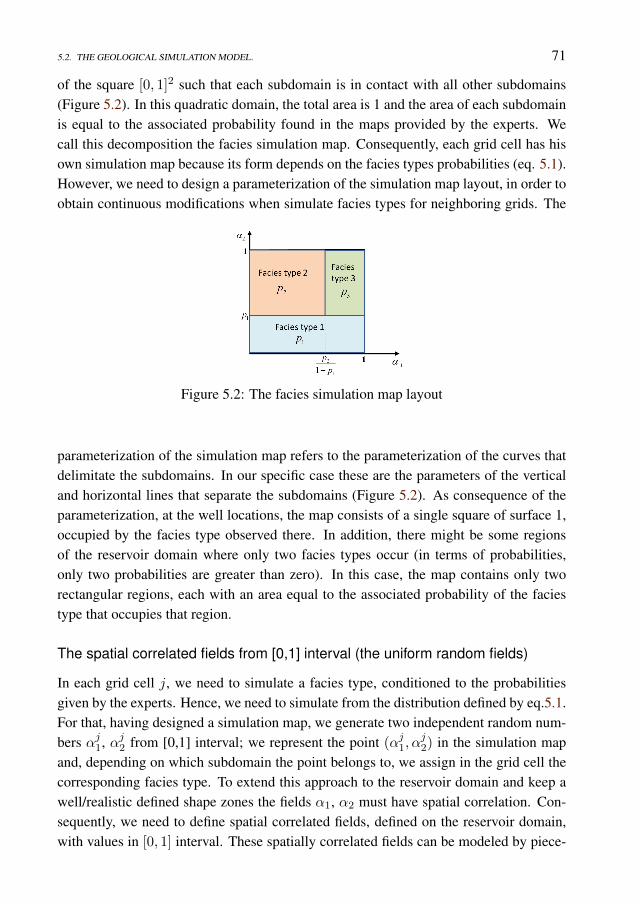
5.2. THE GEOLOGICAL SIMULATION MODEL. 71
of the square [0, 1]2 such that each subdomain is in contact with all other subdomains(Figure 5.2). In this quadratic domain, the total area is 1 and the area of each subdomainis equal to the associated probability found in the maps provided by the experts. Wecall this decomposition the facies simulation map. Consequently, each grid cell has hisown simulation map because its form depends on the facies types probabilities (eq. 5.1).However, we need to design a parameterization of the simulation map layout, in order toobtain continuous modifications when simulate facies types for neighboring grids. The
Figure 5.2: The facies simulation map layout
parameterization of the simulation map refers to the parameterization of the curves thatdelimitate the subdomains. In our specific case these are the parameters of the verticaland horizontal lines that separate the subdomains (Figure 5.2). As consequence of theparameterization, at the well locations, the map consists of a single square of surface 1,occupied by the facies type observed there. In addition, there might be some regionsof the reservoir domain where only two facies types occur (in terms of probabilities,only two probabilities are greater than zero). In this case, the map contains only tworectangular regions, each with an area equal to the associated probability of the faciestype that occupies that region.
The spatial correlated fields from [0,1] interval (the uniform random fields)
In each grid cell j, we need to simulate a facies type, conditioned to the probabilitiesgiven by the experts. Hence, we need to simulate from the distribution defined by eq.5.1.For that, having designed a simulation map, we generate two independent random num-bers αj1, αj2 from [0,1] interval; we represent the point (αj1, α
j2) in the simulation map
and, depending on which subdomain the point belongs to, we assign in the grid cell thecorresponding facies type. To extend this approach to the reservoir domain and keep awell/realistic defined shape zones the fields α1, α2 must have spatial correlation. Con-sequently, we need to define spatial correlated fields, defined on the reservoir domain,with values in [0, 1] interval. These spatially correlated fields can be modeled by piece-
72 CHAPTER 5. THE ADAPTIVE PLURIGAUSSIAN SIMULATION
wise projection into [0,1] of any continuous distributed, spatial correlated random fieldsdefined on the reservoir domain. The condition to be satisfied is that in each grid cell, atthe initial ensemble simulation, the distribution of the variable "facies type" calculatedfrom the ensemble, has to be consistent with the given distribution (eq.5.1). This con-dition is fulfilled if each component of the spatial correlated field (from [0,1] interval)is drawn from an uniform distribution with support on [0,1] interval. Consequently, wecall these spatial correlated fields uniform random fields. In order to define these spatialcorrelated fields we use the probability integral transform (Casella and Berger (2002)[5]). The probability integral transform states that if X is a continuous random variablewith the cumulative distribution function FX , then the random variable FX(X) has anuniform distribution on [0, 1]. The cumulative distribution function links any continuousrandom variable with the uniformly distributed random variable on [0, 1]. Therefore, wecan define the spatial correlated fields (having values in [0, 1]) as piece-wise projectionof any spatial correlated fields (defined on the reservoir domain), of which distributionis continuous, through their cumulative distribution function. We choose to model thesefields as piece-wise Gaussian fields projection because of two important reasons:
1. The generation of the Gaussian random fields can be done easily using any geo-statistical tool.
2. The HM method used in this study (the EnKF) works well under the Gaussianassumption of the model parameters.
In this study we use two properties of the cumulative distribution function (cdf ). The firstproperty is to transfer the geostatistical properties of the Gaussian fields to the spatialcorrelated fields from the [0, 1] interval; the second property is the consequence theprobability integral transform. The projection with cdf ensures that, at the initial stepof facies fields generation the probability map of each facies type is consistent with theoriginals.
The geological simulation model (the APS)
The geological simulation model defined in the plurigaussian context that samples fromprior facies probability maps can be summarise as follows:
1. Design the layout and the parameterization of the facies simulation map.
2. Generate samples of two independent and unconditioned Gaussian random fieldsdefined on the reservoir domain, denoted y1 and y2.
3. Calculate the spatial correlated fields (uniform random fields) α1 = cdf(y1) andα2 = cdf(y2) projecting component-wise the Gaussian fields in [0, 1] using thecdf of the normal distribution used for the Gaussian fields generation.

5.2. THE GEOLOGICAL SIMULATION MODEL. 73
4. Define a facies type in each grid cell j of the reservoir domain.
• Design the facies simulation map associated to grid cell j using the parametriza-tion of the simulation map.
• Assign the facies type associated to the subdomain, in which the realization(αj1, α
j2) falls in the simulation map.
We call this geological simulation model the adaptive plurigaussian simulation model(APS). The simulation scheme is adaptive in the sense that each grid cell has his ownsimulation map, depending on the pair of probabilities. At the well locations the sim-ulation will provide each time the same facies type observed there, because the [0, 1]2
square is completely occupied by a single facies type. However, the main result of thesimulation model is that, if we generate an ensemble of unconditioned and independentpairs of Gaussian fields, the facies probability maps calculated from the ensemble areconsistent with the maps provided by the experts. This can be observed with a visualinspection of the Figure 5.3. At the top of this figure are presented the prior probabilitymaps of the facies occurrence that comes from expert knowledge (the same maps withthe ones presented in Figure 5.1) and at the bottom of the figure the probability mapscalculated from an ensemble of 120 facies fields realizations generated with the APSmodel. This result is the consequence of the lemma presented in the Appendix of the
Figure 5.3: The probability map of each facies type provided by the experts (top) andthe probability maps calculated from an ensemble of realizations (bottom)
paper coupled with the Monte Carlo approach of sampling from Gaussian distributions.The APS model can be generalized to as many facies type we want, to any types of
74 CHAPTER 5. THE ADAPTIVE PLURIGAUSSIAN SIMULATION
contact between facies types. For that, all we have to do is to define a reliable decom-position (parameterization) of the [0, 1]2 square. If the connectivity is very complex wemay carry out the decomposition to higher dimension, using the domain [0, 1]3 and threeGaussian fields for facies maps simulation.
5.2.3 The impact of the facies simulation map
The geological acceptability of the simulated facies distributions is achieved by a reli-able choice of the geostatistical properties of the Gaussian fields and of the simulationmap layout. Usually, in the plurigaussian simulation model, the geostatistical propertiesof the Gaussian fields used for facies simulation are set based on the prior topologicalcharacteristics available for the facies types. We refer here at the geometry of the faciestype, the number of the facies (rock bodies) that occurs in domain and the orientation ofthe facies.In the following, we present an example where, small changes of the simulation maplayout, yield different topological characteristics for the simulated facies maps, whenpreserved the geostatistical properties of the Gaussian fields unchanged. The contactamong facies types can be handled by a reliable definition of the decomposition of theunitary domain. However, the relative position among facies types cannot be handledwith any decomposition. Figure 5.4 shows four possible realizations of the facies distri-butions for reservoirs characterized by the existence of three different rock types, whereany two could be in contact with each other. The green facies type is characterized bylong anisotropy of which angle with the horizontal direction is obtuse. In contrast, thered facies type is characterized by a large amount of small bodies within the reservoirdomain. The blue facies type is the geological environment in which the other two fa-cies types are propagated. These geological realizations were generated using the samevalues of two Gaussian random fields, the first is anisotropic with long range correlationof 50 grid cells, short range correlation of 5 grid cells and with the principal directionof 120 with the horizontal. The second Gaussian random field was generated isotropicwith a small range correlation of 5 grid cells. The parameterization and the layout of thefacies simulation maps are presented at the bottom part of Figure 5.4. We have appliedthe adaptive plurigaussian simulation model, using uniform probability maps of 0.4 forthe facies type 1 (blue) and type 2 (green) and respectively 0.2 for the facies type 3 (red).Even though there are small differences among the simulation map layouts, the facies re-alizations provided exhibit different topological properties. We refer here at the relativeposition of the red facies type with respect to the all facies types. In the first simulation,bodies of the red facies type can be inside both the green and blue facies types. In thesecond example, we may find bodies of the red facies type within the blue facies type,whereas the green facies type intersects the red facies type only on its border. In the third
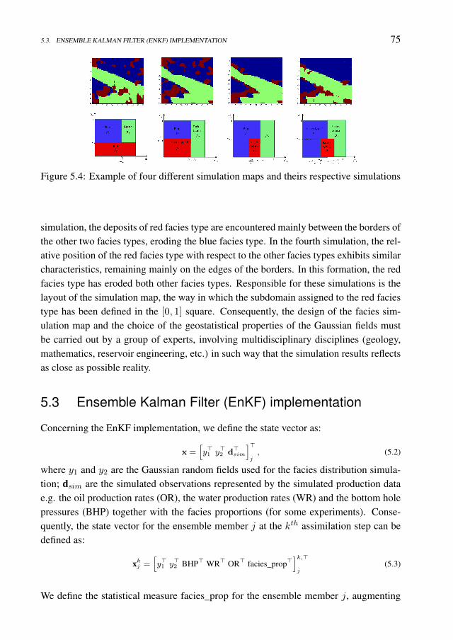
5.3. ENSEMBLE KALMAN FILTER (ENKF) IMPLEMENTATION 75
Figure 5.4: Example of four different simulation maps and theirs respective simulations
simulation, the deposits of red facies type are encountered mainly between the borders ofthe other two facies types, eroding the blue facies type. In the fourth simulation, the rel-ative position of the red facies type with respect to the other facies types exhibits similarcharacteristics, remaining mainly on the edges of the borders. In this formation, the redfacies type has eroded both other facies types. Responsible for these simulations is thelayout of the simulation map, the way in which the subdomain assigned to the red faciestype has been defined in the [0, 1] square. Consequently, the design of the facies sim-ulation map and the choice of the geostatistical properties of the Gaussian fields mustbe carried out by a group of experts, involving multidisciplinary disciplines (geology,mathematics, reservoir engineering, etc.) in such way that the simulation results reflectsas close as possible reality.
5.3 Ensemble Kalman Filter (EnKF) implementation
Concerning the EnKF implementation, we define the state vector as:
x =[y>1 y>2 d>sim
]>j, (5.2)
where y1 and y2 are the Gaussian random fields used for the facies distribution simula-tion; dsim are the simulated observations represented by the simulated production datae.g. the oil production rates (OR), the water production rates (WR) and the bottom holepressures (BHP) together with the facies proportions (for some experiments). Conse-quently, the state vector for the ensemble member j at the kth assimilation step can bedefined as:
xkj =[y>1 y>2 BHP> WR> OR> facies_prop>
]k,>j
(5.3)
We define the statistical measure facies_prop for the ensemble member j, augmenting
76 CHAPTER 5. THE ADAPTIVE PLURIGAUSSIAN SIMULATION
the facies proportions calculated for each facies type i according to
facies_propij =
1
ng
ng∑k=1
Indi(k) (5.4)
the summation being performed for all grid cells (ng grid cells), where the indicatorfunction that express the belonging of the grid cell k to the facies type i is calculated as
Indi(k) =
1 if k ∈ facies type i
0 if k /∈ facies type i(5.5)
The state vector does not contain the petrophysical properties (permeability, porosity) ofthe facies type because we keep these values constant throughout assimilation period.We assume that the uncertainty in the system is due the poorly knowledge of the faciesdistribution in the field. The dynamical variables (the pressure and the saturation) arenot updated together with the parameters because after each assimilation time we havechosen to rerun the simulator from time zero, even though this technique will increasethe computational cost. This avoids the unphysical values of the dynamical parameters(e.g. negative pressures and saturations or saturations greater than 1) in the EnKF updateand the inconsistency between the dynamical variables and the statical variables e.g.the permeability, porosity (the updated dynamical variables could not by an acceptablenumerical solution of the partial differential equations describing the multi-phase flow,given the statical parameters). For small models used in our study this procedure isnot very time consuming, but for large-scale models, the computational cost should beconsidered.
5.3.1 The Work Flow
• InitializationThe uncertainty of the initial ensemble is given by the choice of the model pa-rameters, which in our case are the Gaussian fields y1 and y2. Initially, we gener-ate an ensemble of independent and unconditioned (stationary) pairs of Gaussianfields y1 and y2 (we have used the sequential Gaussian simulation technique im-plemented in S-GeMS [17]). In this study, the stationary Gaussian fields weregenerated with zero mean function, Gaussian covariance type and with each com-ponent having standard normal distribution. Then, using the adaptive plurigaus-sian simulation (APS) model, we generate the initial ensemble of facies maps. Inthis study, we have used 120 ensemble members in all the examples presented.The independence and the unconstraint properties of the Gaussian fields ensuresgeneration of an ensemble of facies maps that represent accurately the prior un-certainty in the facies distribution (Figure 5.3).
5.3. ENSEMBLE KALMAN FILTER (ENKF) IMPLEMENTATION 77
• Forecast step/Model updateWe populate each facies map with proper petrophysical properties (permeability,porosity, etc.). In this study we have chosen to keep constant these values withineach facies not taking into account the heterogeneity within each facies. For eachensemble member we apply the forward model from time zero until the next as-similation time. The forecasted state vector at time k + 1 can be written as:
xk+1,fj =
[yf,>1 yf,>2 BHPf,>WRf,> ORf,> facies_propf,>
]k+1,>
j,
where
[y1y2
]k+1,f
j
=
[y1y2
]k,aj
(5.6)
[p
s
]k+1,f
j
= M
[ p
s
]k0
,
[y1y2
]k,aj
(5.7)
BHPWROR
k+1,f
j
= gpred
[ p
s
]k+1,f
j
,
[y1y2
]k+1,f
j
(5.8)
[facies_prop
]k+1,f
j=
[facies_prop
]k,aj
(5.9)
where gpred is the prediction operator for the production data. Hence, there areno changes from time k to k + 1 for the values of the Gaussian random fields(eq. 5.6), because the forward model equations does not influence the Gaussianfields values. However, their values have an impact in the changes of the pres-sures and saturations at time k + 1 based on the model (eq. 5.7) which generateschanges in the forecast of the production data (eq. 5.8). This happens because theGaussian fields values influence the spatial distribution of the permeability andporosity that generates modification of the dynamical variables (eq. 5.7) and ofthe production data (oil and water rates and pressures at the bottom of wells, eq.5.8). The Gaussian fields values are adapted in the update step of the EnKF whenthe measurements are assimilated. The predicted values for the facies proportionswill not changed, because the facies maps are not adapted during the forecast step(eq. 5.9).
• Update step/Measurement updateAt each assimilation time k+1, k ∈ 0, . . . , ni−1 (ni is the number of the assim-ilation time steps) we assimilate the data (production data and facies proportions)
78 CHAPTER 5. THE ADAPTIVE PLURIGAUSSIAN SIMULATION
using the Kalman filter equations. Each ensemble member is modified accordingto:
xk+1,aj = xk+1,f
j + Cfxk+1H>k+1
(Hk+1C
f
xk+1H>k+1 + Cobs,k+1
)−1
[dobsj ,k+1
−Hk+1xk+1,fj
], (5.10)
where H represents observation operator for the observed data, Cobs representsthe error covariance matrix for the observed data, Cxf represents the forecasted er-ror covariance of the ensemble, and dobsj are the observed data (production dataand facies proportions) of the ensemble member j
• The updated facies mapsThe update of the state vector using the measurements, implies modification ofthe Gaussian fields values (according to eq. 5.10). This update of the Gaussianfields values will change the facies maps. The updated facies maps are obtained bysimulation from the probability maps given by the experts, but using the updatedvalues of the Gaussian fields (conditioned to measurements). This means that wepreserve the simulation maps designed at the beginning throughout assimilationprocess.Consequently, at this step, for each ensemble member i, at each grid cell j weassign the facies type depending on where the updated realization(cdf((ya1)ji , cdf((ya2)ji ) belongs in the simulation map designed for the grid cellj (cdf is the cumulative distribution function of the normal distribution used forgeneration of the Gaussian fields before any data assimilation is performed i.e. thecdf of the standard normal variables).
At the end of the assimilation period, we have obtained an ensemble of facies mapsfrom which we calculate the updated probability map for each facies type. In addition,we have the uncertainty quantification for the geology description provided by the up-dated ensemble of the facies maps. The initial ensemble of the Gaussian fields pairshas initially a high variability (the Gaussian fields are generated unconditioned and in-dependent) which decrease with the assimilation of the production data and facies data(in this case the facies proportions). The variability of the Gaussian field ensemble canbe quantified using an indicator that measures its mean variance:
σ2Y =
1
ng (ne − 1)
ne∑j=1
ng∑i=1
(Y ji − Yi
)2(5.11)
5.4. CASE STUDIES 79
where, ng is the number of the grids, ne is the number of the ensemble members and Yiis the mean value of the random field Y in the grid i
Yi =1
ne
ne∑j=1
Y ji (5.12)
We calculate the mean variance, independently for both Gaussian fields y1 and y2, plot-ting theirs evolution during the assimilation period. The evolution of this indicator pro-vides information about the convergence or collapse of the ensemble (Agbalaka andOliver 2008, Sebacher et al 2013).
5.4 Case studies
In this section, we present two applications of the adaptive plurigaussian simulationmethod. In the first example we consider a reservoir where three facies types occur, anytwo of them could be in contact with the others. Schematically, we may represent thesecharacteristics as F1 ⇔ F2, F2 ⇔ F3 and F3 ⇔ F1. In the second example, we presenta case where in the reservoir four facies types occur, while two of the facies types do nothave contact. For both cases presented, we consider the geostatistical properties of theGaussian fields and the layout of the facies simulation map known. The reference fieldsand the prior probability maps of the facies occurrence are generated with the geologicalsimulation model presented in Sebacher et al. 2013 .
5.4.1 The model with three facies types
We consider a model with three facies types with the distribution presented in the pre-vious sections. We perform two experiments. In first experiment, we consider as mea-surements only the pressure at the injector and the oil and water rates at the producers.In the second experiment, we introduce as measurement the facies proportions. The ex-perts have knowledge about these values, together with a uncertainty bandwidth whichare translated into stochastic elements as measurement errors for facies proportions.The simulation model is a 5-spot water flooding 2D-reservoir, black oil model with50× 50× 1 active grid cells. The dimension of each grid cell was set at 30× 30× 20 ftand there is one injector situated at the center of the reservoir domain and there are fourproducers situated at the corners. The coordinates of the wells positions are presentedin Table 5.1 and the facies observations are presented in Table 5.1. The values of thepermeability and porosity corresponding to each facies type are shown in Table 5.2.
Water injection starts from the first day and continue thereafter a period of 201 daysof production. We assimilate data starting from first day until day 201, with 10-day in-terval, having 21 assimilation steps. All the producers work under constant BHP valueof 1500 pound per square inch (psi), the injector operates at 4500 stock tank barrels per
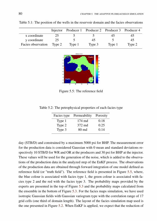
80 CHAPTER 5. THE ADAPTIVE PLURIGAUSSIAN SIMULATION
Table 5.1: The position of the wells in the reservoir domain and the facies observations
Injector Producer 1 Producer 2 Producer 3 Producer 4x coordinate 25 5 5 45 45y coordinate 25 5 45 5 45
Facies observation Type 2 Type 1 Type 3 Type 1 Type 2
Figure 5.5: The reference field
Table 5.2: The petrophysical properties of each facies type
Facies type Permeability PorosityType 1 174 md 0.18Type 2 372 md 0.25Type 3 80 md 0.14
day (STB/D) and constrained by a maximum 5000 psi for BHP. The measurement errorfor the production data is considered Gaussian with 0 mean and standard deviations re-spectively 10 STB/D for WR and OR at the producers and 30 psi for BHP at the injector.These values will be used for the generation of the noise, which is added to the observa-tions of the production data in the analyzed step of the EnKF process. The observationsof the production data are obtained through forward integration of one model defined asreference field (or "truth field"). The reference field is presented in Figure 5.5, where,the blue colour is associated with facies type 1, the green colour is associated with fa-cies type 2 and the red with the facies type 3. The probability maps provided by theexperts are presented in the top of Figure 5.3 and the probability maps calculated fromthe ensemble in the bottom of Figure 5.3. For the facies maps simulation, we have usedisotropic Gaussian fields with Gaussian variogram type with the correlation range of 17grid cells (one third of domain length). The layout of the facies simulation map used isthe one presented in Figure 5.2. When EnKF is applied, we expect that the reduction of
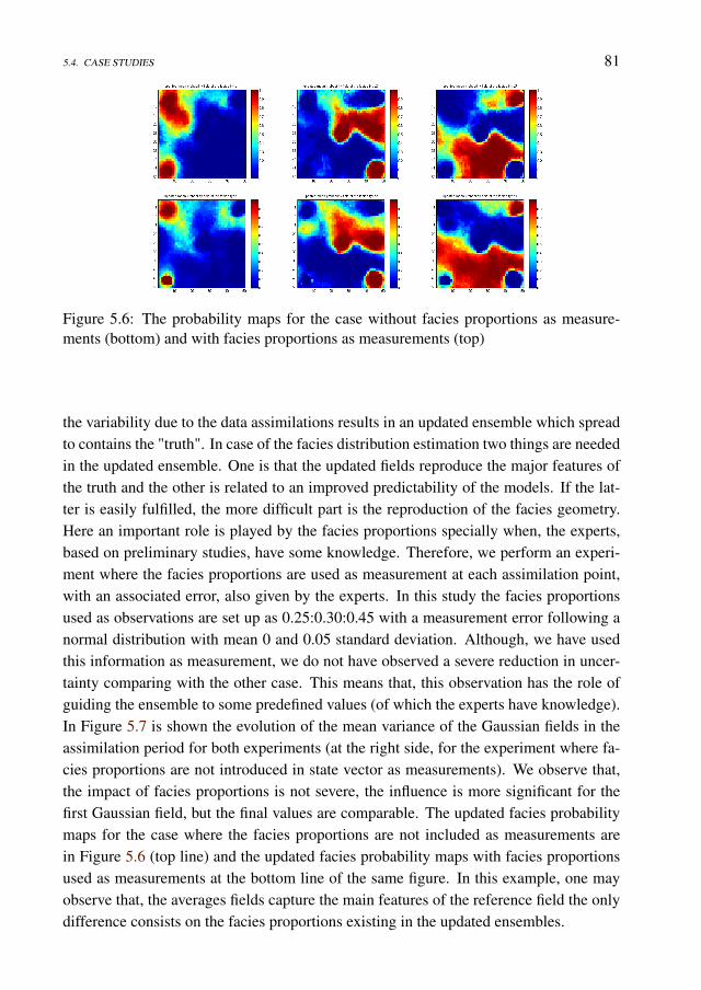
5.4. CASE STUDIES 81
Figure 5.6: The probability maps for the case without facies proportions as measure-ments (bottom) and with facies proportions as measurements (top)
the variability due to the data assimilations results in an updated ensemble which spreadto contains the "truth". In case of the facies distribution estimation two things are neededin the updated ensemble. One is that the updated fields reproduce the major features ofthe truth and the other is related to an improved predictability of the models. If the lat-ter is easily fulfilled, the more difficult part is the reproduction of the facies geometry.Here an important role is played by the facies proportions specially when, the experts,based on preliminary studies, have some knowledge. Therefore, we perform an experi-ment where the facies proportions are used as measurement at each assimilation point,with an associated error, also given by the experts. In this study the facies proportionsused as observations are set up as 0.25:0.30:0.45 with a measurement error following anormal distribution with mean 0 and 0.05 standard deviation. Although, we have usedthis information as measurement, we do not have observed a severe reduction in uncer-tainty comparing with the other case. This means that, this observation has the role ofguiding the ensemble to some predefined values (of which the experts have knowledge).In Figure 5.7 is shown the evolution of the mean variance of the Gaussian fields in theassimilation period for both experiments (at the right side, for the experiment where fa-cies proportions are not introduced in state vector as measurements). We observe that,the impact of facies proportions is not severe, the influence is more significant for thefirst Gaussian field, but the final values are comparable. The updated facies probabilitymaps for the case where the facies proportions are not included as measurements arein Figure 5.6 (top line) and the updated facies probability maps with facies proportionsused as measurements at the bottom line of the same figure. In this example, one mayobserve that, the averages fields capture the main features of the reference field the onlydifference consists on the facies proportions existing in the updated ensembles.
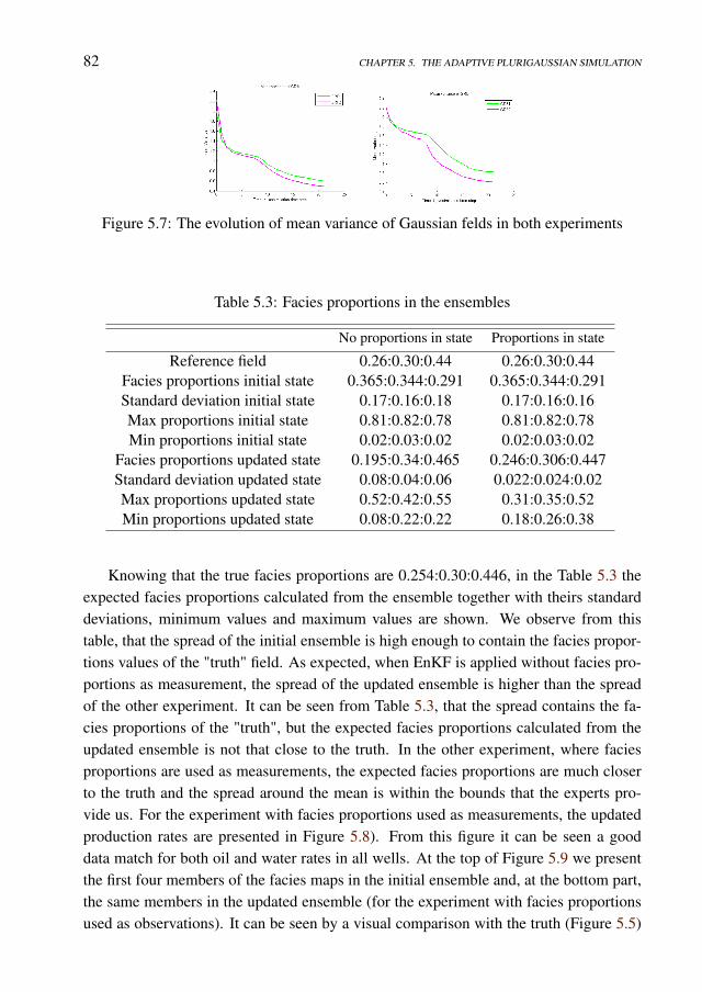
82 CHAPTER 5. THE ADAPTIVE PLURIGAUSSIAN SIMULATION
Figure 5.7: The evolution of mean variance of Gaussian felds in both experiments
Table 5.3: Facies proportions in the ensembles
No proportions in state Proportions in state
Reference field 0.26:0.30:0.44 0.26:0.30:0.44Facies proportions initial state 0.365:0.344:0.291 0.365:0.344:0.291Standard deviation initial state 0.17:0.16:0.18 0.17:0.16:0.16Max proportions initial state 0.81:0.82:0.78 0.81:0.82:0.78Min proportions initial state 0.02:0.03:0.02 0.02:0.03:0.02
Facies proportions updated state 0.195:0.34:0.465 0.246:0.306:0.447Standard deviation updated state 0.08:0.04:0.06 0.022:0.024:0.02Max proportions updated state 0.52:0.42:0.55 0.31:0.35:0.52Min proportions updated state 0.08:0.22:0.22 0.18:0.26:0.38
Knowing that the true facies proportions are 0.254:0.30:0.446, in the Table 5.3 theexpected facies proportions calculated from the ensemble together with theirs standarddeviations, minimum values and maximum values are shown. We observe from thistable, that the spread of the initial ensemble is high enough to contain the facies propor-tions values of the "truth" field. As expected, when EnKF is applied without facies pro-portions as measurement, the spread of the updated ensemble is higher than the spreadof the other experiment. It can be seen from Table 5.3, that the spread contains the fa-cies proportions of the "truth", but the expected facies proportions calculated from theupdated ensemble is not that close to the truth. In the other experiment, where faciesproportions are used as measurements, the expected facies proportions are much closerto the truth and the spread around the mean is within the bounds that the experts pro-vide us. For the experiment with facies proportions used as measurements, the updatedproduction rates are presented in Figure 5.8). From this figure it can be seen a gooddata match for both oil and water rates in all wells. At the top of Figure 5.9 we presentthe first four members of the facies maps in the initial ensemble and, at the bottom part,the same members in the updated ensemble (for the experiment with facies proportionsused as observations). It can be seen by a visual comparison with the truth (Figure 5.5)
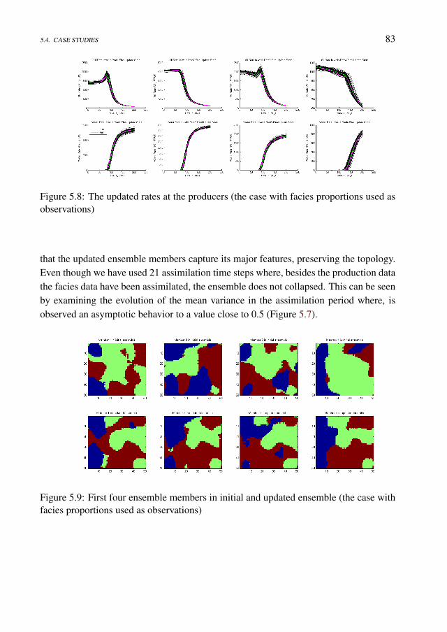
5.4. CASE STUDIES 83
Figure 5.8: The updated rates at the producers (the case with facies proportions used asobservations)
that the updated ensemble members capture its major features, preserving the topology.Even though we have used 21 assimilation time steps where, besides the production datathe facies data have been assimilated, the ensemble does not collapsed. This can be seenby examining the evolution of the mean variance in the assimilation period where, isobserved an asymptotic behavior to a value close to 0.5 (Figure 5.7).
Figure 5.9: First four ensemble members in initial and updated ensemble (the case withfacies proportions used as observations)
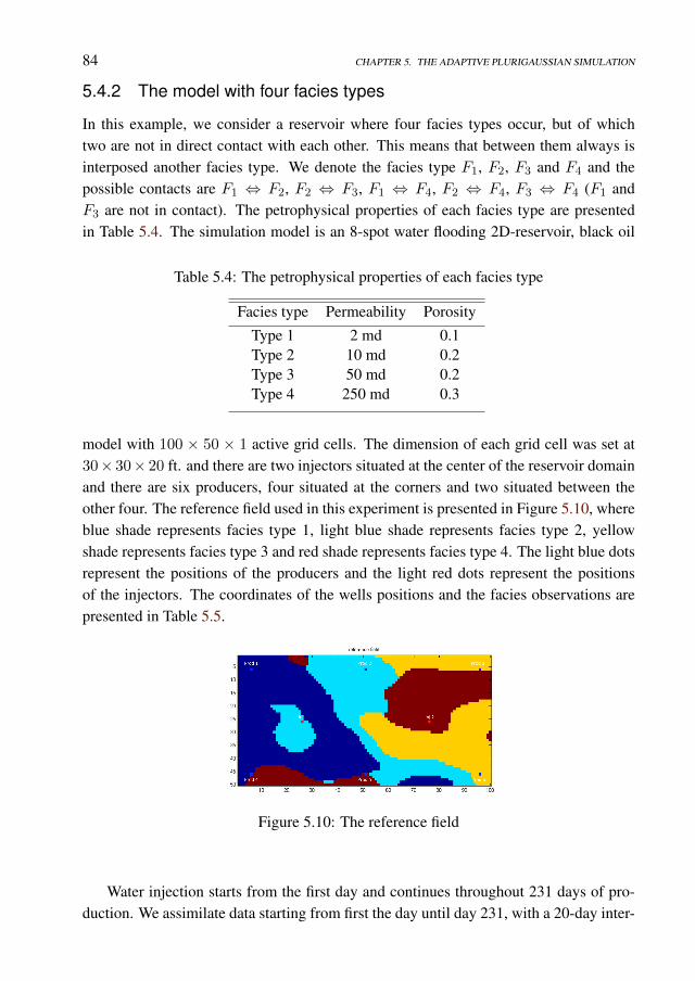
84 CHAPTER 5. THE ADAPTIVE PLURIGAUSSIAN SIMULATION
5.4.2 The model with four facies types
In this example, we consider a reservoir where four facies types occur, but of whichtwo are not in direct contact with each other. This means that between them always isinterposed another facies type. We denote the facies type F1, F2, F3 and F4 and thepossible contacts are F1 ⇔ F2, F2 ⇔ F3, F1 ⇔ F4, F2 ⇔ F4, F3 ⇔ F4 (F1 andF3 are not in contact). The petrophysical properties of each facies type are presentedin Table 5.4. The simulation model is an 8-spot water flooding 2D-reservoir, black oil
Table 5.4: The petrophysical properties of each facies type
Facies type Permeability PorosityType 1 2 md 0.1Type 2 10 md 0.2Type 3 50 md 0.2Type 4 250 md 0.3
model with 100 × 50 × 1 active grid cells. The dimension of each grid cell was set at30× 30× 20 ft. and there are two injectors situated at the center of the reservoir domainand there are six producers, four situated at the corners and two situated between theother four. The reference field used in this experiment is presented in Figure 5.10, whereblue shade represents facies type 1, light blue shade represents facies type 2, yellowshade represents facies type 3 and red shade represents facies type 4. The light blue dotsrepresent the positions of the producers and the light red dots represent the positionsof the injectors. The coordinates of the wells positions and the facies observations arepresented in Table 5.5.
Figure 5.10: The reference field
Water injection starts from the first day and continues throughout 231 days of pro-duction. We assimilate data starting from first the day until day 231, with a 20-day inter-
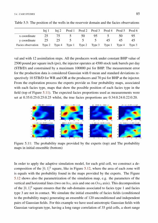
5.4. CASE STUDIES 85
Table 5.5: The position of the wells in the reservoir domain and the facies observations
Inj 1 Inj 2 Prod 1 Prod 2 Prod 3 Prod 4 Prod 5 Prod 6
x coordinate 25 75 5 50 95 5 50 95y coordinate 25 25 5 5 5 45 45 45
Facies observation Type 2 Type 4 Type 1 Type 2 Type 3 Type 1 Type 4 Type 3
val and with 12 assimilation steps. All the producers work under constant BHP value of2500 pound per square inch (psi), the injector operates at 4500 stock tank barrels per day(STB/D) and constrained by a maximum 100000 psi for BHP. The measurement errorfor the production data is considered Gaussian with 0 mean and standard deviations re-spectively 10 STB/D for WR and OR at the producers and 70 psi for BHP at the injector.From the exploration process the experts provide us four probability maps, associatedwith each facies type, maps that show the possible position of each facies type in thefield (top of Figure 5.11). The expected facies proportions used as measurements wereset at 0.35:0.25:0.25:0.25 whilst, the true facies proportions are 0.34:0.24:0.22:0.20.
Figure 5.11: The probability maps provided by the experts (top) and The probabilitymaps in initial ensemble (bottom)
In order to apply the adaptive simulation model, for each grid cell, we construct a de-composition of the [0, 1]2 square, like in Figure 5.12, where the area of each zone willis equals with the probability found in the maps provided by the experts. The Figure5.12 shows also the parametrization of the simulation map, e.g. the parameters of thevertical and horizontal lines (two on 0α1 axis and one onOα2 axis). This decompositionof the [0, 1]2 square ensures that the sub-domains associated to facies type 1 and faciestype 3 are not in contact. We simulate the initial ensemble of facies fields (conditionedto the probability maps) generating an ensemble of 120 unconditioned and independentpairs of Gaussian fields. For this example we have used anisotropic Gaussian fields withGaussian variogram type, having a long range correlation of 35 grid cells, a short range
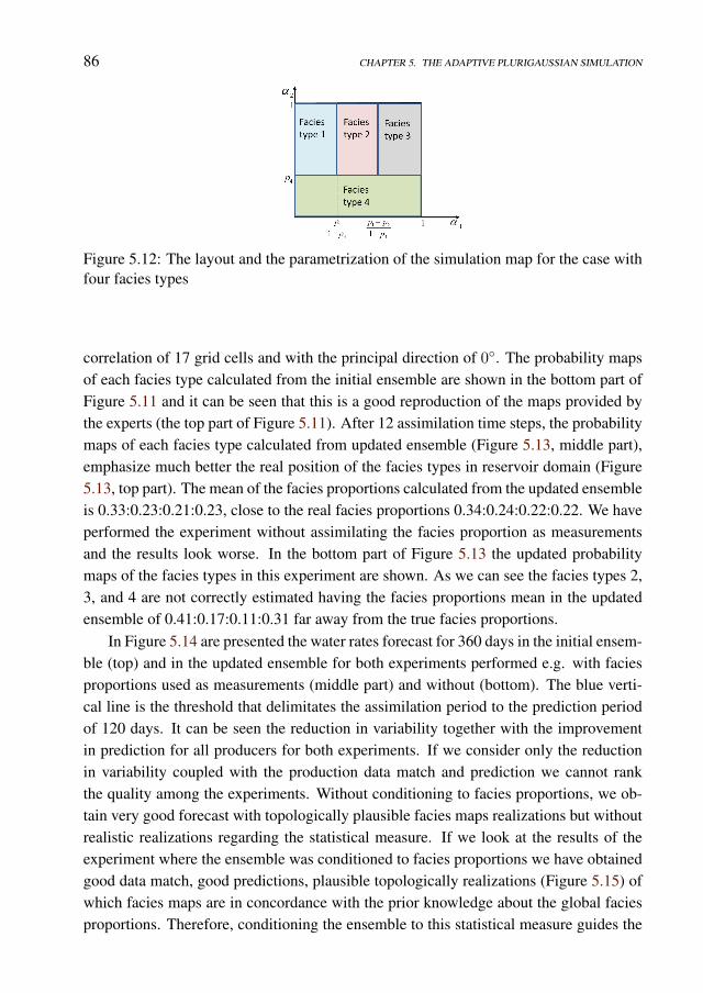
86 CHAPTER 5. THE ADAPTIVE PLURIGAUSSIAN SIMULATION
Figure 5.12: The layout and the parametrization of the simulation map for the case withfour facies types
correlation of 17 grid cells and with the principal direction of 0. The probability mapsof each facies type calculated from the initial ensemble are shown in the bottom part ofFigure 5.11 and it can be seen that this is a good reproduction of the maps provided bythe experts (the top part of Figure 5.11). After 12 assimilation time steps, the probabilitymaps of each facies type calculated from updated ensemble (Figure 5.13, middle part),emphasize much better the real position of the facies types in reservoir domain (Figure5.13, top part). The mean of the facies proportions calculated from the updated ensembleis 0.33:0.23:0.21:0.23, close to the real facies proportions 0.34:0.24:0.22:0.22. We haveperformed the experiment without assimilating the facies proportion as measurementsand the results look worse. In the bottom part of Figure 5.13 the updated probabilitymaps of the facies types in this experiment are shown. As we can see the facies types 2,3, and 4 are not correctly estimated having the facies proportions mean in the updatedensemble of 0.41:0.17:0.11:0.31 far away from the true facies proportions.
In Figure 5.14 are presented the water rates forecast for 360 days in the initial ensem-ble (top) and in the updated ensemble for both experiments performed e.g. with faciesproportions used as measurements (middle part) and without (bottom). The blue verti-cal line is the threshold that delimitates the assimilation period to the prediction periodof 120 days. It can be seen the reduction in variability together with the improvementin prediction for all producers for both experiments. If we consider only the reductionin variability coupled with the production data match and prediction we cannot rankthe quality among the experiments. Without conditioning to facies proportions, we ob-tain very good forecast with topologically plausible facies maps realizations but withoutrealistic realizations regarding the statistical measure. If we look at the results of theexperiment where the ensemble was conditioned to facies proportions we have obtainedgood data match, good predictions, plausible topologically realizations (Figure 5.15) ofwhich facies maps are in concordance with the prior knowledge about the global faciesproportions. Therefore, conditioning the ensemble to this statistical measure guides the
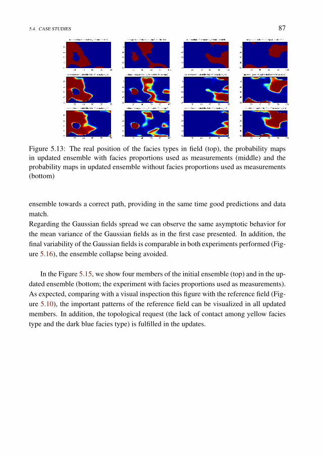
5.4. CASE STUDIES 87
Figure 5.13: The real position of the facies types in field (top), the probability mapsin updated ensemble with facies proportions used as measurements (middle) and theprobability maps in updated ensemble without facies proportions used as measurements(bottom)
ensemble towards a correct path, providing in the same time good predictions and datamatch.Regarding the Gaussian fields spread we can observe the same asymptotic behavior forthe mean variance of the Gaussian fields as in the first case presented. In addition, thefinal variability of the Gaussian fields is comparable in both experiments performed (Fig-ure 5.16), the ensemble collapse being avoided.
In the Figure 5.15, we show four members of the initial ensemble (top) and in the up-dated ensemble (bottom; the experiment with facies proportions used as measurements).As expected, comparing with a visual inspection this figure with the reference field (Fig-ure 5.10), the important patterns of the reference field can be visualized in all updatedmembers. In addition, the topological request (the lack of contact among yellow faciestype and the dark blue facies type) is fulfilled in the updates.
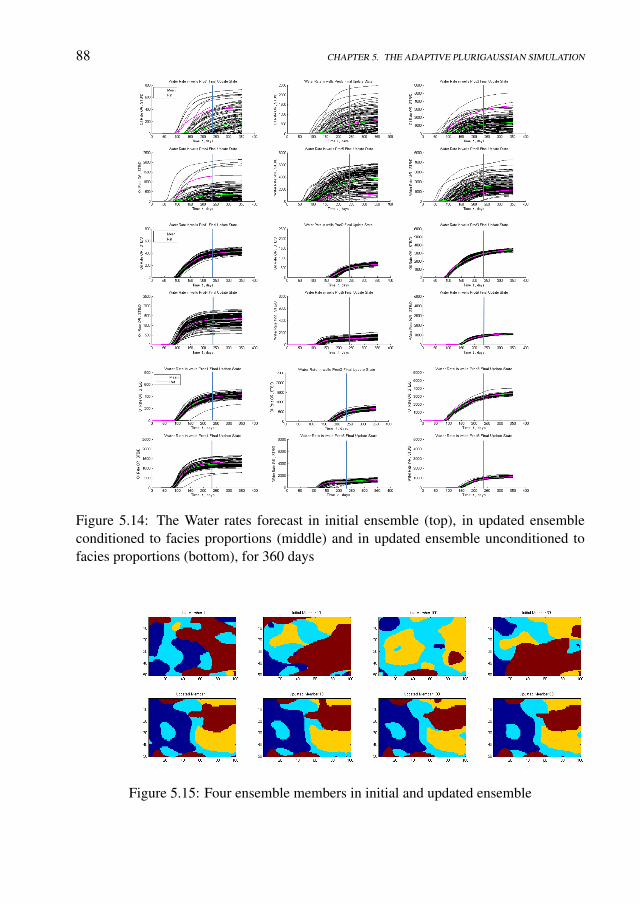
88 CHAPTER 5. THE ADAPTIVE PLURIGAUSSIAN SIMULATION
Figure 5.14: The Water rates forecast in initial ensemble (top), in updated ensembleconditioned to facies proportions (middle) and in updated ensemble unconditioned tofacies proportions (bottom), for 360 days
Figure 5.15: Four ensemble members in initial and updated ensemble
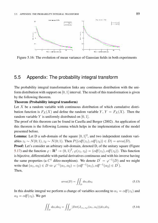
5.5. APPENDIX: THE PROBABILITY INTEGRAL TRANSFORM 89
Figure 5.16: The evolution of mean variance of Gaussian fields in both experiments
5.5 Appendix: The probability integral transform
The probability integral transformation links any continuous distribution with the uni-form distribution with support on [0, 1] interval. The result of this transformation is givenby the following theorem.Theorem (Probability integral transform)Let X be a random variable with continuous distribution of which cumulative distri-bution function is FX(X) and define the random variable Y , Y = FX(X). Then therandom variable Y is uniformly distributed on [0, 1].The proof of this theorem can be found in Casella and Berger (2002). An application ofthis theorem is the following Lemma which helps in the implementation of the modelpresented before.Lemma: Let D a sub-domain of the square [0, 1]2, and two independent random vari-ables z1 ∼ N(0; 1), z2 ∼ N(0; 1). Then P ((cdf(z1), cdf(z2)) ∈ D) = area(D).Proof: Let’s consider an arbitrary sub-domain, denoted D, of the unitary square (Figure5.17) and the function ϕ : R2 → (0, 1)2, ϕ(z1, z2) = (cdf(z1), cdf(z2)). This functionis bijective, differentiable with partial derivatives continuous and with his inverse havingthe same properties (a C1 difeo-morphism). We denote D
′= ϕ−1(D) and we might
write that (α1, α2) ∈ D ⇔ ϕ−1(α1, α2) = (cdf−1(α1), cdf−1(α2) ∈ D′).Then,
area(D) =
∫∫D
dα1dα2 (5.13)
In this double integral we perform a change of variables according to α1 = cdf(z1) andα2 = cdf(z2). We get
∫∫D
dα1dα2 =
∫∫D′|Det(J(z1,z2)(α1, α2))|dz1dz2 (5.14)
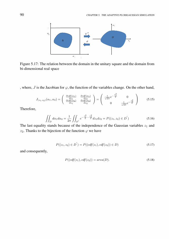
90 CHAPTER 5. THE ADAPTIVE PLURIGAUSSIAN SIMULATION
Figure 5.17: The relation between the domain in the unitary square and the domain frombi-dimensional real space
, where, J is the Jacobian for ϕ, the function of the variables change. On the other hand,
J(z1,z2)(α1, α2) =
(∂cdf(α1)∂z1
∂cdf(α1)∂z2
∂cdf(α2)∂z1
∂cdf(α2)∂z2
)=
1√2πe−
z212 0
0 1√2πe−
z222
(5.15)
Therefore, ∫∫D
dα1dα2 =1
2π
∫∫D′e−
z212−z222 dz1dz2 = P ((z1, z2) ∈ D
′) (5.16)
The last equality stands because of the independence of the Gaussian variables z1 andz2. Thanks to the bijection of the function ϕ we have
P ((z1, z2) ∈ D′) = P ((cdf(z1), cdf(z2)) ∈ D) (5.17)
and consequently,
P ((cdf(z1), cdf(z2)) = area(D). (5.18)
Chapter 6
Bridging multiple pointgeostatistics and truncatedGaussian fields for improvedestimation of channelizedreservoirs with ensemble methods
6.1 Introduction
An important key in reservoirs engineering is the development of reliable reservoir mod-els with high predictive capacity of production behavior in existing and potentially newdrilled wells. The reservoir predictability is the starting point for guiding the productionplan to an optimum. In order to achieve this, the geological description plays a crucialrole. The initial description of the subsurface fields, such as permeability and porosity,could be carried out using geostatistical tools in specialized modules, defining thus, thesimulation model and its uncertainty. When referred to a geological description of thereservoir, one may think of a description of the spatial distribution of the petrophysicalproperties (permeability and/or porosity) or more natural, a description of the spatialdistribution of the geological deposits formations (facies). Prior information is relatedto the types of the facies that are collected in the initial stage of subsurface description.Based on this prior information, a reliable geological simulation model is chosen in order
This chapter is full reference of an article submitted to Computational Geosciences
91
92 CHAPTER 6. CHANNELIZED RESERVOIRS
to generate realistic reservoir instances. The geological simulation model can be definedeither using object based simulation technique (Deutsch and Journel, 1998; Deutsch andWang, 1996) or grid based simulation techniques such as the multi-point geostatistics(MPS)(Guardiano and Srivastava, 1993; Strebelle, 2002; Caers and Zhang, 2004) andalso, the truncated pluri-Gaussian methods (TPS) (Galli et al., 1994) Irrespective of thegeological simulation model used, the poor knowledge of geology leads to an initialreservoir model whose parameters are uncertain. This prior uncertainty is usually solarge that the predictive capacity is limited. To improve the predictive capacity, the prioruncertainty is reduced in a process named in reservoir engineering as history matching(HM), either manual or assisted. Comprehensive description of some assisted historymatching methods can be found in Oliver et al. (2008). This paper addresses the casewhere the subsurface is characterized by the presence of two facies types, of which oneinhabits channelized geometry. This type of spatial distribution is hardly obtained usingTPS simulation techniques, especially because of the TPS restriction of applicability tovariogram models. More appropriate is the use of MPS simulation methods such as thesingle normal equation simulation method (SNESIM, Strebelle (2002)). These geosta-tistical tools enable generations of more complex and natural instances of facies distri-butions, relying on a general conceptual structural model (a training image) of whichconstruction incorporates the prior knowledge of the subsurface geometry and topol-ogy. By combining ideas from permeability updates in an MPS setting (Jafarpour andKhodabakhshi, 2011) with a Gaussian parameterization of the marginal facies probabili-ties, we define a TPS method where the truncation map is estimated from samples usingMPS and a training image. This allows for non-Gaussian dependence structures and weavoid pre-specification of a variogram/covariance function and truncation map. One ofthe most commonly used assisted HM methods is the ensemble Kalman filter (Evensen,1994. 2003; Aanonsen et al., 2009) especially for its ease of implementation and itsdesign to work with an ensemble of models instead of a single model. However, sincethe direct use of the facies types petrophysical properties (permeability and/or porosity)as model parameters does not conducts the EnKF process to geological realistic updatesdue to the Gaussian nature of the method, a (re)parameterization of the facies field isneeded. In Sarma et al. (2008) a parameterization of the log-permeability fields (definedby the facies field), with kernel principal component analysis (PCA) methodology, car-ried out in a high-dimensional space was proposed. The link between the input space(the space where the K-L expansion were performed) and the feature space is realizedthrough a nonlinear function where an inner product is defined by a kernel function. Theauthors used a polynomial kernel of order two or three. In Sarma et al. (2009) the EnKFis applied in the high-dimensional feature space, in which the log-permeability fieldswere carried with mapping functions, whose kernels are of polynomial type. For theupdates, a back transform defined via a pre-image problem has to be solved. The results
6.1. INTRODUCTION 93
showed improvement in preserving of the high order statistical moments of the updates;this could be seen in the random field continuity. However, because the parameterizationinvolved the permeability fields the updates are not facies fields. Therefore, the posterioruncertainty refer to the log-permeability distribution uncertainty, not facies distributionuncertainty. Another unsolved issue with the kernel EnKF method is it’s tendency forall the ensemble members to collapse onto a single model. A different approach inquantification of the permeability distribution uncertainty is presented in Jafarpour etal. (2007). The authors proposed a parameterization of the log-permeability, pressureand saturation fields using the Fourier discrete cosine transform (DCT) and coupled thereservoir model with EnKF for history matching. The results showed an improvementin the random field connectivity compared with the HM process applied directly to log-permeability fields. The facies distribution uncertainty quantification could be achievedwith the parametrization of the facies fields using level set methods as in Lorentzen etal. (2009) were a level set function is used to assign a signed distance to the channelborder, the positive sign being reserved for the grid cells inside of the channel, whereas,the other grid cells have negative distance values. Then, the EnKF is used for updatingof the distance fields, generated after comparing it with the zero field. In the contextof the MPS simulation models, Hu et al. (2013) proposed the parametrization of a uni-form random field used for the simulation of a certain facies types at grid cells, based onthe conditional probability distributions extracted from the training image. The Gaus-sian transformation of such uniform field is further updated with the EnKF, the resultsshowed an improved uncertainty quantification of the facies distribution. Other faciesparameterizations which involve the domain transformation have been proposed, suchas, the discrete wavelet transform (Jafarpour, 2011) or the gradual deformation (Rog-gero and Hu, 1998). The choice of the MPS as geological simulation model is based onthe information collected at the initial stage of reservoir description. However, if impor-tant data are revealed, such as core information (hard data) or information from seismicsurveillance (soft data), this information can easily be incorporated in the MPS model us-ing probabilistic models (Journel, 2002; Krishnan et al., 2005). The challenge, however,is how to incorporate dynamical production data. In Caers and Hoffman (2006) a model(the probability perturbation method, PPM) that links the dynamical (flow) measure-ments with the MPS geological simulation model is developed. The sampling from theprior model (represented by the training image) rely on a the "tau" probabilistic model(Journel, 2002), by perturbing a so called pre-posterior probability (the probability ofoccurrence of a facies type given the "dynamical" data). The pre-posterior perturbationis carried out with a convex relation that depends on a sub-unitary parameter estimationwhich involves an optimization procedure of the square misfit between the measurementsand the response. The process is iterative because multiple random seeds should be usedin order for the simulations to match the data. An ensemble based method that links
94 CHAPTER 6. CHANNELIZED RESERVOIRS
the dynamical data with the MPS simulation model was develop in Jafarpour and Khod-abakhshi (2011). The authors propose a probability conditioning method (PCM) forfacies simulation in the context of EnKF as HM method. The initial ensemble of faciesrealization are drawn from the training image conditioned on a uniform probability mapand equal weights. At each assimilation point, the log-permeability fields are updatedusing the available measurements, with the EnKF, and, from the mean log-permeabilityfield, updated probability maps for each facies type are inferred. Piece-wise linear func-tions have been used to project the mean log-permeability field to the probability field.Then, another initial ensemble is drawn from the prior model, using the tau model forconditioning the training image on the updated facies probability maps. This procedurewill continue until the end of the assimilation period. The final ensemble has a realisticgeometry structure (being drawn from training image) with a reduced data mismatch.However, the piece-wise linear assumption between the log-permeability and facies oc-currence probability has an empirical component and the variability and the randomnessintroduced by the MPS model does not ensures a good data match in the updates. At thesame time, the model is highly dependent on the permeability estimation from EnKF,so if there is not enough information in the data to detect facies from the updated log-permeability field , the procedure may fail. In other words it relies on the EnKF’s abilityto detect features in the continuous permeability field, which may not be the case ifmeasurements in the reservoir domain is sparse, as is typical for real fields. This is incontrast to most of the proposed methodology discussed here, were the number of wellsis large compared to the reservoir size. We present a new parametrization of the faciesfields, in the context of MPS geological simulation model, which is further coupled withthe iterative adaptive Gaussian mixture (Stordal and Lorentzen, 2014) for uncertaintyquantification of the channelized reservoirs. The parameterization bridges ideas fromMPS and TPS. The standard TPS parameterization ensures that the updated fields arefacies fields, however, since the field is jointly Gaussian it is not trivial to characterizechannel type facies structures via a covariance function (or variogram) in combinationwith a user defined truncation map. The MPS approach has the advantage of simulatingchannel type random fields, however, they are discrete-valued and it is not trivial to con-nect this with ensemble based inversion. We therefor suggest a combination of the twoparameterizations. By estimating marginal facies probabilities from a sample from MPSin combination with a training image, we parameterize the marginal probability fieldwith a (marginally) Gaussian random field where the truncation map is defined such thatthe integral for a facies type in a given grid cell in the Gaussian domain coincides withmarginal grid cell facies probability estimated from the ensemble. This automaticallygives us a truncation map in the Gaussian space that honors the channel structures sincethe dependence structure is inherited from the training image. Thus we can update thecontinuous-valued random field using any ensemble based history matching technique
6.1. INTRODUCTION 95
and change the facies type in each grid cell according to the truncation map. This en-sures us that the updated ensemble members are always facies fields. However, sinceall ensemble based methods are only approximating the Bayesian solution, the updatedfields are not from the correct posterior distribution for these nonlinear problems. Typi-cally, after an update, the non Gaussian prior is violated in the sense that the facies fieldshave discontinuous channels. We address this problem in two ways, first instead of us-ing the EnKF we apply the recently published iterative adaptive Gaussian mixture filter.For non Gaussian models, this method is asymptotically better than any EnKF approachsince the bias can be controlled. Secondly, it has a resampling step between iterations.The resampling allows us to combine this resampling step with the resampling usingthe updated probability fields estimated from the updated ensemble and the MPS as inJafarpour and Khodabakhshi (2011), to better preserve channels. In addition this allowsus to resample ensemble members using MPS after all data is assimilated in contrast tothe EnKF approach where resampling is performed after each assimilation step. Afterresampling, a new iteration with AGM (Stordal et al., 2011) is then performed usingthe resampled ensemble as initial ensemble. After two or three iterations, the updatedensemble of facies maps remains geologically realistic, even without resampling, henceafter the final iteration, we are left with ensemble members that have continuous channelstructures and match the data. Placed in the context of the already existing parameter-ization we might also consider it as being a level set type, but the thresholds used forfacies delimitation have a spatial distribution. This spatial distribution is given by theinitial ensemble of realizations drawn from the training image. In Section 6.2 we intro-duced and described in details the new parameterization of the facies field. In Section6.3 the history matching algorithm used (IAGM) is summarized and its advantages overmore traditional techniques are presented. This is followed by simulation studies in Sec-tion 6.4 where we performed two experiments with synthetic 2D reservoirs of varyingsize. The first is a channelized reservoir model with 50*50 grid cells and the second has100*100 grid cells. For the first experiment, a comparison with EnKF was performed inorder to emphasize the benefits of the iterative method. Secondly, IAGM is also appliedto update the permeability directly and then compute a probability map (Jafarpour andKhodabakhshi, 2011). This is to show that improvements are due to the combination ofIAGM and the new parameterization and not IAGM alone. The second experiment withthe reservoir model having 10000 grid cells, only the IAGM with the new parameteriza-tion is shown as the conclusion is the same as for the experiment.

96 CHAPTER 6. CHANNELIZED RESERVOIRS
6.2 Parameterization and truncation in the Gaussian space
A parametrization of the elements of a given set Y could be defined as a surjective func-tion φ : X → Y , where X is a metric space. In our case Y is represented by the space offacies maps. Usually, if n is the dimension of the reservoir domain, X ⊆ Rn×k, where kis a positive integer number. When a HM method is applied, the values in the X -spaceare changed and, using the function φ, a new facies distribution is provided. The rea-son for using φ is to ensure that the updated ensemble members are facies realizations.When the facies fields are directly populated with petrophysical properties (permeability,porosity, etc.) the updated values does not easily back transform to facies realizationswhen ensemble methods such as EnKF or AGM are applied. Therefore a parametriza-tion of the facies field is needed. One possibility is to truncate the permeability fields,however, this would requires a user specified truncation map. Further, when working di-rectly with permeability fields, the updated fields are no longer facies fields hence thereis an intrinsic need for truncation after the update which may violate the quality of thedata match. Truncated (pluri) Gaussian fields also requires a user defined truncationmap, however, given this map, the updated fields are guaranteed to be facies fields. TheTPS method however is not capable of handling channel structures.
Here we introduce a truncated marginal Gaussian parameterization for channelizedreservoirs with two facies types, although extension to more facies types is almoststraight forward. The only problem with multiple facies is that the truncation map,estimated from the ensemble, is not unique. However, the facies proportions are directlyestimated from an initial sample and the dependence structure is inherited from the train-ing image and do not requires specification. In other words, the new parameterizationconsists of continuous valued random fields that are marginally Gaussian and where thejoint distribution depends on the MPS tool used to generate initial facies models. Thegeological simulation model used is in this work is SNESIM, where a training imageis used to generate initial ensembles of facies fields. In the following we present a pa-rameterization of the facies field in a Gaussian space and the transformation function(truncation rule) φ that transforms elements in the Gaussian space to elements in thespace of facies fields.
Let us consider an initial ensemble of facies fields (channelized fields) generatedusing the prior knowledge of the reservoir subsurface characterization. We denote thenumber of the ensemble members by ne. From the ensemble, we estimate, in each gridcell, the marginal probability of the channel type facies. For grid cell i the estimate isgiven by the proportion of the ensemble that has channel in gird cell i. Then, if pi is theestimated probability of the channel occurrence, the distribution of the random variable,
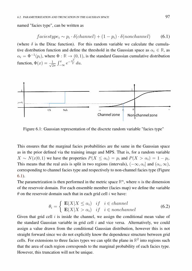
6.2. PARAMETERIZATION AND TRUNCATION IN THE GAUSSIAN SPACE 97
named "facies type", can be written as
faciestypei ∼ pi · δ(channel) + (1− pi) · δ(nonchannel) (6.1)
(where δ is the Dirac function). For this random variable we calculate the cumula-tive distribution function and define the threshold in the Gaussian space as αi ∈ R, asαi = Φ−1(pi), where Φ : R → (0, 1), is the standard Gaussian cumulative distribution
function, Φ(x) = 1√2π
∫ x−∞ e
−u2
2 du.
Figure 6.1: Gaussian representation of the discrete random variable "facies type"
This ensures that the marginal facies probabilities are the same in the Gaussian spaceas in the prior defined via the training image and MPS. That is, for a random variableX ∼ N(x|0, 1) we have the properties P (X ≤ αi) = pi and P (X > αi) = 1 − pi.This means that the real axis is split in two regions (intervals), (−∞, αi] and (αi,∞),corresponding to channel facies type and respectively to non-channel facies type (Figure6.1).The parametrization is then performed in the metric space Rn, where n is the dimensionof the reservoir domain. For each ensemble member (facies map) we define the variableθ on the reservoir domain such that in each grid cell i we have:
θi =
E(X|X ≤ αi) if i ∈ channelE(X|X > αi) if i ∈ nonchannel (6.2)
Given that grid cell i is inside the channel, we assign the conditional mean value ofthe standard Gaussian variable in grid cell i and vice versa. Alternatively, we couldassign a value drawn from the conditional Gaussian distribution, however this is notstraight forward since we do not explicitly know the dependence structure between gridcells. For extensions to three facies types we can split the plane in R2 into regions suchthat the area of each region corresponds to the marginal probability of each facies type.However, this truncation will not be unique.

98 CHAPTER 6. CHANNELIZED RESERVOIRS
Consequently, the function φ may be defined asφ : Rn → K1,K0n, where,
φ(θ) =
K1 if θi ≤ αiK0 if θi > αi
(6.3)
for any grid cell i. In this definition, K1 and K0 are represent the permeability valuefor each facies type in FM, the set of facies maps defined on the reservoir domain wherethe subindex 1 represents the channel and 0 the non-channel facies type. The function φcan, in the same manner, easily be extended to other petrophysical variables such as e.g.porosity. By construction we see that E(θ) ≡ 0 since, in grid cell i, we have
E (θi) = piE(X|X ≤ αi) + (1− pi)E(X|X > αi)
= pi(Φ(αi))−1
∫ αi
−∞x
1√2π
exp
(−1
2x2)dx
= +(1− pi)(1− Φ(αi))−1
∫ −∞αi
x1√2π
exp
(−1
2x2)dx
=
∫ ∞−∞
x1√2π
exp
(−1
2x2)dx = 0,
where we have used that Φ(αi) = pi.
Figure 6.2: The pdf of the Gaussian variables
As a consequence the marginal prior mean of the parameter field with mean 0 ineach grid cell (Figure 6.3, last picture). These conditional means have also a physicalinterpretation, as the gravity centers of the associated intervals of each facies type withrespect to the density of the standard Gaussian variable (Figure 6.2). For an initial en-semble conditioned to hard data (facies observations at the well locations) for a givennumber of grid cells, these grid cells has θ values 0 with threshold values α = −∞ orα =∞ depending on the type of the observation (nonchannel and respectively channel).If, in the probability map, we have value 0.5 for the channel occurrence then α = 0 andθch = −θnch (θch and θnch are the gravity centers of the interval assigned to the channel
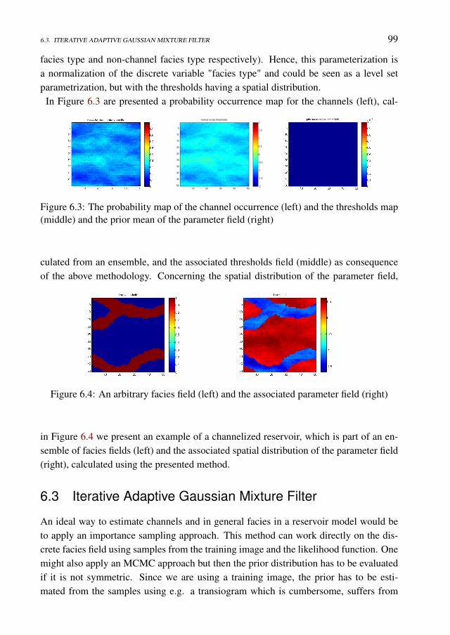
6.3. ITERATIVE ADAPTIVE GAUSSIAN MIXTURE FILTER 99
facies type and non-channel facies type respectively). Hence, this parameterization isa normalization of the discrete variable "facies type" and could be seen as a level setparametrization, but with the thresholds having a spatial distribution.
In Figure 6.3 are presented a probability occurrence map for the channels (left), cal-
Figure 6.3: The probability map of the channel occurrence (left) and the thresholds map(middle) and the prior mean of the parameter field (right)
culated from an ensemble, and the associated thresholds field (middle) as consequenceof the above methodology. Concerning the spatial distribution of the parameter field,
Figure 6.4: An arbitrary facies field (left) and the associated parameter field (right)
in Figure 6.4 we present an example of a channelized reservoir, which is part of an en-semble of facies fields (left) and the associated spatial distribution of the parameter field(right), calculated using the presented method.
6.3 Iterative Adaptive Gaussian Mixture Filter
An ideal way to estimate channels and in general facies in a reservoir model would beto apply an importance sampling approach. This method can work directly on the dis-crete facies field using samples from the training image and the likelihood function. Onemight also apply an MCMC approach but then the prior distribution has to be evaluatedif it is not symmetric. Since we are using a training image, the prior has to be esti-mated from the samples using e.g. a transiogram which is cumbersome, suffers from
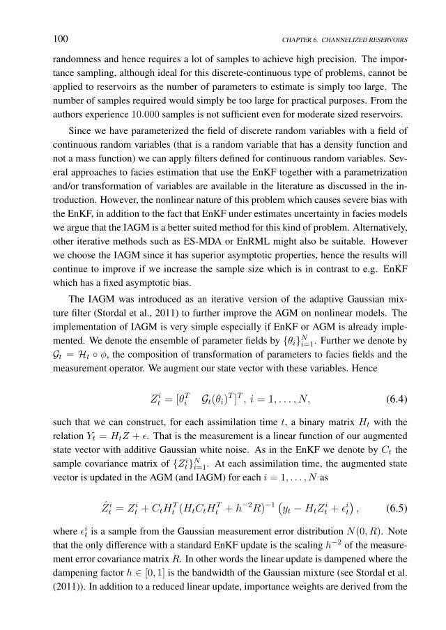
100 CHAPTER 6. CHANNELIZED RESERVOIRS
randomness and hence requires a lot of samples to achieve high precision. The impor-tance sampling, although ideal for this discrete-continuous type of problems, cannot beapplied to reservoirs as the number of parameters to estimate is simply too large. Thenumber of samples required would simply be too large for practical purposes. From theauthors experience 10.000 samples is not sufficient even for moderate sized reservoirs.
Since we have parameterized the field of discrete random variables with a field ofcontinuous random variables (that is a random variable that has a density function andnot a mass function) we can apply filters defined for continuous random variables. Sev-eral approaches to facies estimation that use the EnKF together with a parametrizationand/or transformation of variables are available in the literature as discussed in the in-troduction. However, the nonlinear nature of this problem which causes severe bias withthe EnKF, in addition to the fact that EnKF under estimates uncertainty in facies modelswe argue that the IAGM is a better suited method for this kind of problem. Alternatively,other iterative methods such as ES-MDA or EnRML might also be suitable. Howeverwe choose the IAGM since it has superior asymptotic properties, hence the results willcontinue to improve if we increase the sample size which is in contrast to e.g. EnKFwhich has a fixed asymptotic bias.
The IAGM was introduced as an iterative version of the adaptive Gaussian mix-ture filter (Stordal et al., 2011) to further improve the AGM on nonlinear models. Theimplementation of IAGM is very simple especially if EnKF or AGM is already imple-mented. We denote the ensemble of parameter fields by θiNi=1. Further we denote byGt = Ht φ, the composition of transformation of parameters to facies fields and themeasurement operator. We augment our state vector with these variables. Hence
Zit = [θTi Gt(θi)T ]T , i = 1, . . . , N, (6.4)
such that we can construct, for each assimilation time t, a binary matrix Ht with therelation Yt = HtZ + ε. That is the measurement is a linear function of our augmentedstate vector with additive Gaussian white noise. As in the EnKF we denote by Ct thesample covariance matrix of ZitNi=1. At each assimilation time, the augmented statevector is updated in the AGM (and IAGM) for each i = 1, . . . , N as
Zit = Zi
t + CtHTt (HtCtH
Tt + h−2R)−1
(yt −HtZ
it + εit
), (6.5)
where εit is a sample from the Gaussian measurement error distribution N(0, R). Notethat the only difference with a standard EnKF update is the scaling h−2 of the measure-ment error covariance matrix R. In other words the linear update is dampened where thedampening factor h ∈ [0, 1] is the bandwidth of the Gaussian mixture (see Stordal et al.(2011)). In addition to a reduced linear update, importance weights are derived from the
6.3. ITERATIVE ADAPTIVE GAUSSIAN MIXTURE FILTER 101
Gaussian mixture and updated sequentially as
W it ∝ W i
t−1N(yt −HtZit , h−2HCHT +R). (6.6)
To avoid filter degeneracy that occurs in high dimension and complex systems a weightinterpolation is introduced
WW it = αtW
it + (1− αt)N−1, αt ∈ [0, 1], (6.7)
where
αt = N−1(N∑i=1
(W it )
2)−1. (6.8)
For details of the AGM we refer to Stordal et al. (2011).A resampling and reweighting step in the algorithm before rerunning AGM is dis-
cussed in Stordal and Lorentzen (2014). Here we propose to resample from the trainingimage with a new probability field obtained from the weighted mean of the ensemblemembers after the previous iteration. That is, after one assimilation cycle, a new proba-bility map is constructed on a cell by cell basis as
pi =
ne∑j=1
wj1(celli ∈ channel)
and used in SNESIM . This is equivalent to resampling marginal facies variables from theempirical distribution obtained with AGM (resampling) with the constraint that the de-pendence structure is given by the training image. To be completely rigorous we shouldthen evaluate the ratio between the old and new prior for each ensemble member, how-ever this would requires the estimation of the prior in addition to evaluation of weightsin high dimensions. With the weight reduction leading to almost uniform weights due tothe dimension, there would be more work than gain, and we instead make the assumptionof uniform weights after resampling from the training image with the new probabilityfield. The resampling and reweighting is a topic for future research. In most applicationsa few iterations are required, typically two or three. This is in agreement with the resultswe present below.
6.3.1 The State Vector
Concerning the HM methods implementation, the state vector for the ith ensemble mem-ber at the tth assimilation step will be:
Xit =
[paramT
i Gt(parami)T]T, i = 1, . . . , N (6.9)
where Gt(parami) are the simulated observations represented by the simulated produc-
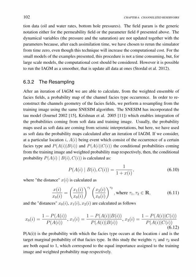
102 CHAPTER 6. CHANNELIZED RESERVOIRS
tion data (oil and water rates, bottom hole pressures). The field param is the genericnotation either for the permeability field or the parameter field θ presented above. Thedynamical variables (the pressure and the saturation) are not updated together with theparameters because, after each assimilation time, we have chosen to rerun the simulatorfrom time zero, even though this technique will increase the computational cost. For thesmall models of the examples presented, this procedure is not a time consuming, but, forlarge scale models, the computational cost should be considered. However it is possibleto run the IAGM as a smoother, that is update all data at ones (Stordal et al. 2012).
6.3.2 The Resampling
After an iteration of IAGM we are able to calculate, from the weighted ensemble offacies fields, a probability map of the channel facies type occurrence. In order to re-construct the channels geometry of the facies fields, we perform a resampling from thetraining image using the same SNESIM algorithm. The SNESIM has incorporated thetau model (Journel 2002 [15], Krishnan et al. 2005 [11]) which enables integration ofthe probabilities coming from soft data and training image. Usually, the probabilitymaps used as soft data are coming from seismic interpretations, but here, we have usedas soft data the probability maps calculated after an iteration of IAGM. If we consider,at a particular location i, A(i) being event which consist of the occurrence of a certainfacies type and P (A(i)|B(i)) and P (A(i)|C(i)) the conditional probabilities comingfrom the training image and weighted probability map respectively, then, the conditionalprobability P (A(i) | B(i), C(i)) is calculated as:
P (A(i) | B(i), C(i)) =1
1 + x(i), (6.10)
where "the distance" x(i) is calculated as
x(i)
x0(i)=
(x1(i)
x0(i)
)τ1 (x2(i)
x0(i)
)τ2,where τ1, τ2 ∈ R, (6.11)
and the "distances" x0(i), x1(i), x2(i) are calculated as follows
x0(i) =1− P (A(i))
P (A(i)), x1(i) =
1− P (A(i)|B(i))
P (A(i)|B(i)), x2(i) =
1− P (A(i)|C(i))
P (A(i)|C(i))(6.12)
P(A(i)) is the probability with which the facies type occurs at the location i and is thetarget marginal probability of that facies type. In this study the weights τ1 and τ2 usedare both equal to 1, which correspond to the equal importance assigned to the trainingimage and weighted probability map respectively.
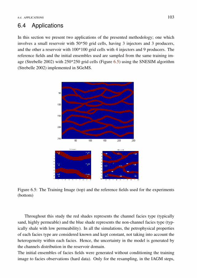
6.4. APPLICATIONS 103
6.4 Applications
In this section we present two applications of the presented methodology; one whichinvolves a small reservoir with 50*50 grid cells, having 3 injectors and 3 producers,and the other a reservoir with 100*100 grid cells with 4 injectors and 9 producers. Thereference fields and the initial ensembles used are sampled from the same training im-age (Strebelle 2002) with 250*250 grid cells (Figure 6.5) using the SNESIM algorithm(Strebelle 2002) implemented in SGeMS.
Figure 6.5: The Training Image (top) and the reference fields used for the experiments(bottom)
Throughout this study the red shades represents the channel facies type (typicallysand, highly permeable) and the blue shade represents the non-channel facies type (typ-ically shale with low permeability). In all the simulations, the petrophysical propertiesof each facies type are considered known and kept constant, not taking into account theheterogeneity within each facies. Hence, the uncertainty in the model is generated bythe channels distribution in the reservoir domain.The initial ensembles of facies fields were generated without conditioning the trainingimage to facies observations (hard data). Only for the resampling, in the IAGM steps,

104 CHAPTER 6. CHANNELIZED RESERVOIRS
the initial ensembles were generated conditioning the training image to the previous es-timated probability map. The number of iterations in the experiments was establishedtaking into account the properties of the updated ensemble. This should fulfill two re-quirements; good data match and predictions, and the updated ensemble members shouldnot be in conflict with our prior believes, that is, the ensemble should have continuouschannel structures. With that in mind, we terminate the assimilation process when theensemble members are matching the data satisfactory at the same time as they havecontinuous channels. The latter can be achieved by resampling from the training im-age using a probability map projected from the mean permeability field (Jafarpour andKhodabakhshi, 2011), however the quality of the data match is then decreased. Sinceour parameterization is guarantees that our updated ensemble members are facies fields,we do not need to perform resampling after the final iteration. This gives our method anadvantage over previous work.

6.4. APPLICATIONS 105
6.4.1 Channelized reservoir with 2500 grid cells
In this example we present the case of a small channelized 2D reservoir, with 50 gridcells in each direction of which dimension was set at 30 × 30 × 20 ft. We design thereservoir with a 6-spot water flooding black oil model, having three injection wells at theleft side and three production wells at the right side. The reservoir is initially filled withoil at a constant uniform saturation of 0.8 (which generates a connate water saturationof 0.2) and with a uniform pressure of 5000 psi in every grid cell. The producers worksunder constant bottom hole pressure (BHP) value of 1500 psi and the injectors operateat 2500 stock tank barrels per day (STB/D) constrained by a maximum 100000 psi forBHP. The measurement errors of the production data are assumed Gaussian with 0 meanand standard deviations of 30 STB/D for water rates (WR) and oil rates (OR) at theproducers, and 80 psi for BHP at the injectors, respectively. These values are used whengenerating the reference measurements, and also when adding noise to the productiondata in the analyzed step of the HM processes. Water injection starts from the firstday and continues for a period of 191 days. We assimilate data starting from the firstday until day 191, with a 20-day interval, resulting in 10 assimilation steps. For eachexperiment the measurements were obtained through forward simulation of the syntheticmodel presented as the "reference" in which the channels geometry is defined by twonon-intersected narrow bands which propagate longitudinally (Figure 6.5, bottom left).The permeability values were set at 500 mD and 50 mD for the channel facies type andfor the non-channel facies type, respectively, while the porosity of both facies types isconsidered 0.2.In this subsection we perform the following experiments:
• EnKF with log-permeability estimation.
• EnKF with the parameter field.
• IAGM with h=0.25 two iterations and with the parameter field.
In the top of Figure 6.6 the true position of the channels in the field is presented and inthe following pictures we present the prior mean and posterior mean of all the results ofthe experiments. In Figure 6.6(b) the prior mean and posterior mean refer to the meanlog-permeability, whereas for all the rest we refer to the mean probability map of thechannels occurrence.
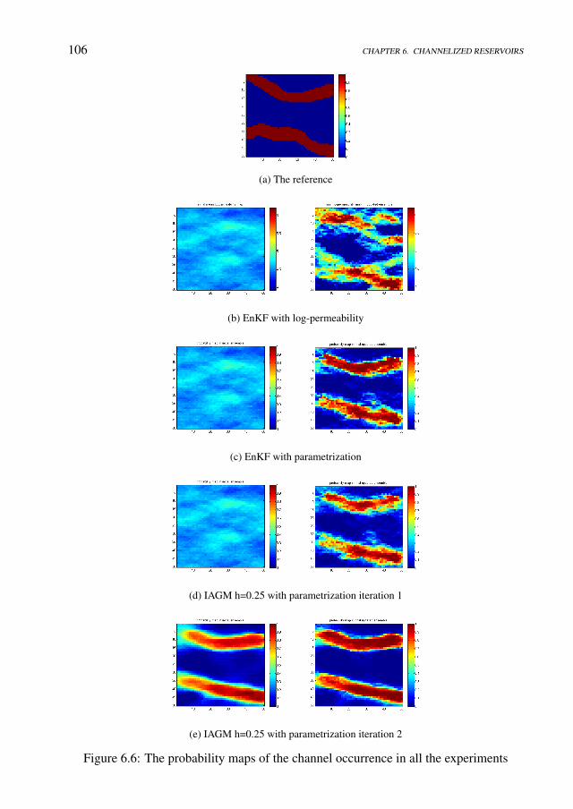
106 CHAPTER 6. CHANNELIZED RESERVOIRS
(a) The reference
(b) EnKF with log-permeability
(c) EnKF with parametrization
(d) IAGM h=0.25 with parametrization iteration 1
(e) IAGM h=0.25 with parametrization iteration 2
Figure 6.6: The probability maps of the channel occurrence in all the experiments
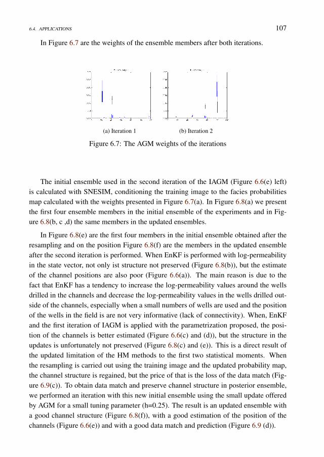
6.4. APPLICATIONS 107
In Figure 6.7 are the weights of the ensemble members after both iterations.
(a) Iteration 1 (b) Iteration 2
Figure 6.7: The AGM weights of the iterations
The initial ensemble used in the second iteration of the IAGM (Figure 6.6(e) left)is calculated with SNESIM, conditioning the training image to the facies probabilitiesmap calculated with the weights presented in Figure 6.7(a). In Figure 6.8(a) we presentthe first four ensemble members in the initial ensemble of the experiments and in Fig-ure 6.8(b, c ,d) the same members in the updated ensembles.
In Figure 6.8(e) are the first four members in the initial ensemble obtained after theresampling and on the position Figure 6.8(f) are the members in the updated ensembleafter the second iteration is performed. When EnKF is performed with log-permeabilityin the state vector, not only ist structure not preserved (Figure 6.8(b)), but the estimateof the channel positions are also poor (Figure 6.6(a)). The main reason is due to thefact that EnKF has a tendency to increase the log-permeability values around the wellsdrilled in the channels and decrease the log-permeability values in the wells drilled out-side of the channels, especially when a small numbers of wells are used and the positionof the wells in the field is are not very informative (lack of connectivity). When, EnKFand the first iteration of IAGM is applied with the parametrization proposed, the posi-tion of the channels is better estimated (Figure 6.6(c) and (d)), but the structure in theupdates is unfortunately not preserved (Figure 6.8(c) and (e)). This is a direct result ofthe updated limitation of the HM methods to the first two statistical moments. Whenthe resampling is carried out using the training image and the updated probability map,the channel structure is regained, but the price of that is the loss of the data match (Fig-ure 6.9(c)). To obtain data match and preserve channel structure in posterior ensemble,we performed an iteration with this new initial ensemble using the small update offeredby AGM for a small tuning parameter (h=0.25). The result is an updated ensemble witha good channel structure (Figure 6.8(f)), with a good estimation of the position of thechannels (Figure 6.6(e)) and with a good data match and prediction (Figure 6.9 (d)).
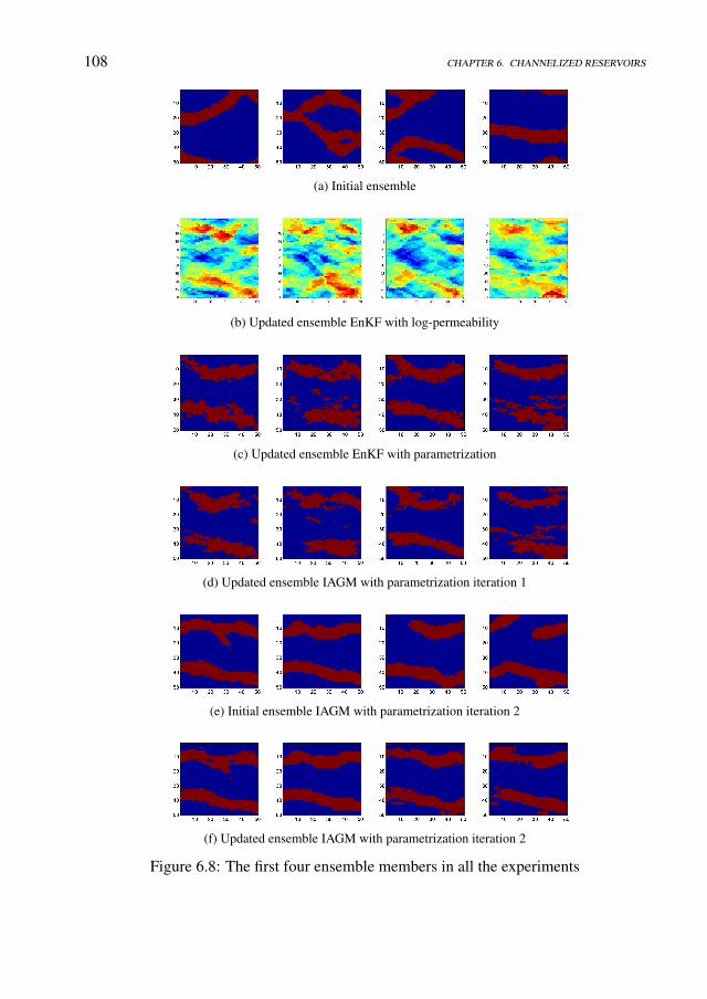
108 CHAPTER 6. CHANNELIZED RESERVOIRS
(a) Initial ensemble
(b) Updated ensemble EnKF with log-permeability
(c) Updated ensemble EnKF with parametrization
(d) Updated ensemble IAGM with parametrization iteration 1
(e) Initial ensemble IAGM with parametrization iteration 2
(f) Updated ensemble IAGM with parametrization iteration 2
Figure 6.8: The first four ensemble members in all the experiments
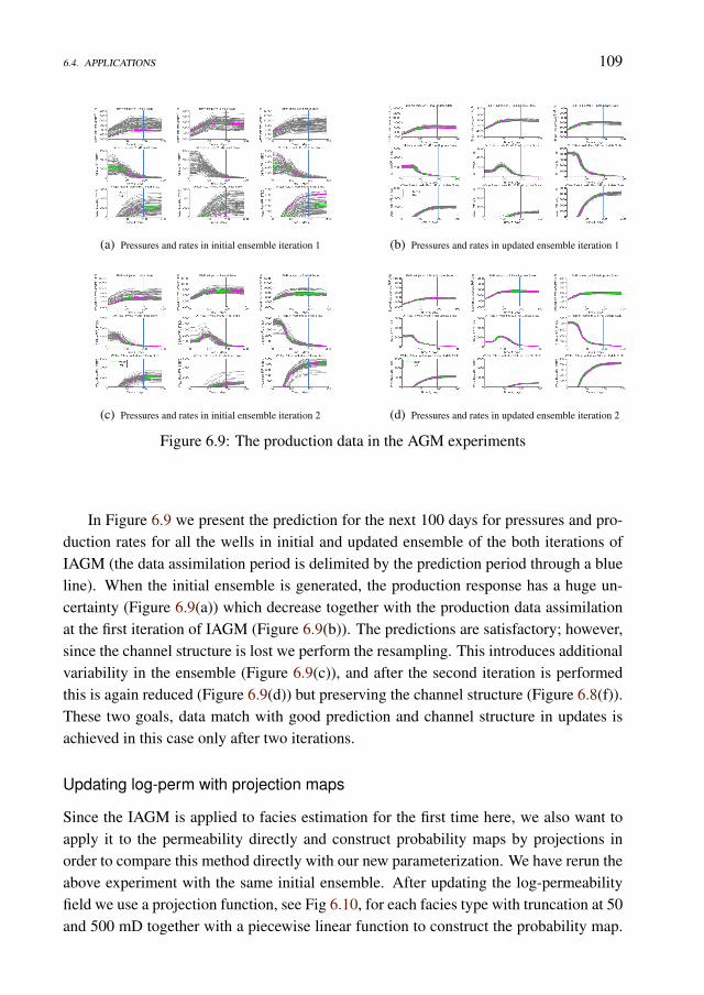
6.4. APPLICATIONS 109
(a) Pressures and rates in initial ensemble iteration 1 (b) Pressures and rates in updated ensemble iteration 1
(c) Pressures and rates in initial ensemble iteration 2 (d) Pressures and rates in updated ensemble iteration 2
Figure 6.9: The production data in the AGM experiments
In Figure 6.9 we present the prediction for the next 100 days for pressures and pro-duction rates for all the wells in initial and updated ensemble of the both iterations ofIAGM (the data assimilation period is delimited by the prediction period through a blueline). When the initial ensemble is generated, the production response has a huge un-certainty (Figure 6.9(a)) which decrease together with the production data assimilationat the first iteration of IAGM (Figure 6.9(b)). The predictions are satisfactory; however,since the channel structure is lost we perform the resampling. This introduces additionalvariability in the ensemble (Figure 6.9(c)), and after the second iteration is performedthis is again reduced (Figure 6.9(d)) but preserving the channel structure (Figure 6.8(f)).These two goals, data match with good prediction and channel structure in updates isachieved in this case only after two iterations.
Updating log-perm with projection maps
Since the IAGM is applied to facies estimation for the first time here, we also want toapply it to the permeability directly and construct probability maps by projections inorder to compare this method directly with our new parameterization. We have rerun theabove experiment with the same initial ensemble. After updating the log-permeabilityfield we use a projection function, see Fig 6.10, for each facies type with truncation at 50and 500 mD together with a piecewise linear function to construct the probability map.
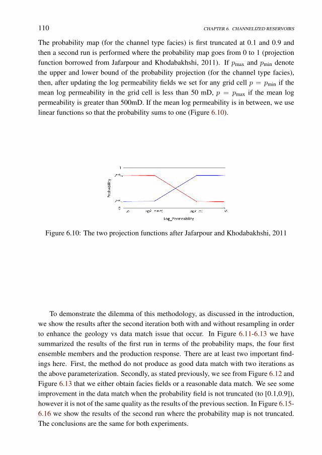
110 CHAPTER 6. CHANNELIZED RESERVOIRS
The probability map (for the channel type facies) is first truncated at 0.1 and 0.9 andthen a second run is performed where the probability map goes from 0 to 1 (projectionfunction borrowed from Jafarpour and Khodabakhshi, 2011). If pmax and pmin denotethe upper and lower bound of the probability projection (for the channel type facies),then, after updating the log permeability fields we set for any grid cell p = pmin if themean log permeability in the grid cell is less than 50 mD, p = pmax if the mean logpermeability is greater than 500mD. If the mean log permeability is in between, we uselinear functions so that the probability sums to one (Figure 6.10).
Figure 6.10: The two projection functions after Jafarpour and Khodabakhshi, 2011
To demonstrate the dilemma of this methodology, as discussed in the introduction,we show the results after the second iteration both with and without resampling in orderto enhance the geology vs data match issue that occur. In Figure 6.11-6.13 we havesummarized the results of the first run in terms of the probability maps, the four firstensemble members and the production response. There are at least two important find-ings here. First, the method do not produce as good data match with two iterations asthe above parameterization. Secondly, as stated previously, we see from Figure 6.12 andFigure 6.13 that we either obtain facies fields or a reasonable data match. We see someimprovement in the data match when the probability field is not truncated (to [0.1,0.9]),however it is not of the same quality as the results of the previous section. In Figure 6.15-6.16 we show the results of the second run where the probability map is not truncated.The conclusions are the same for both experiments.
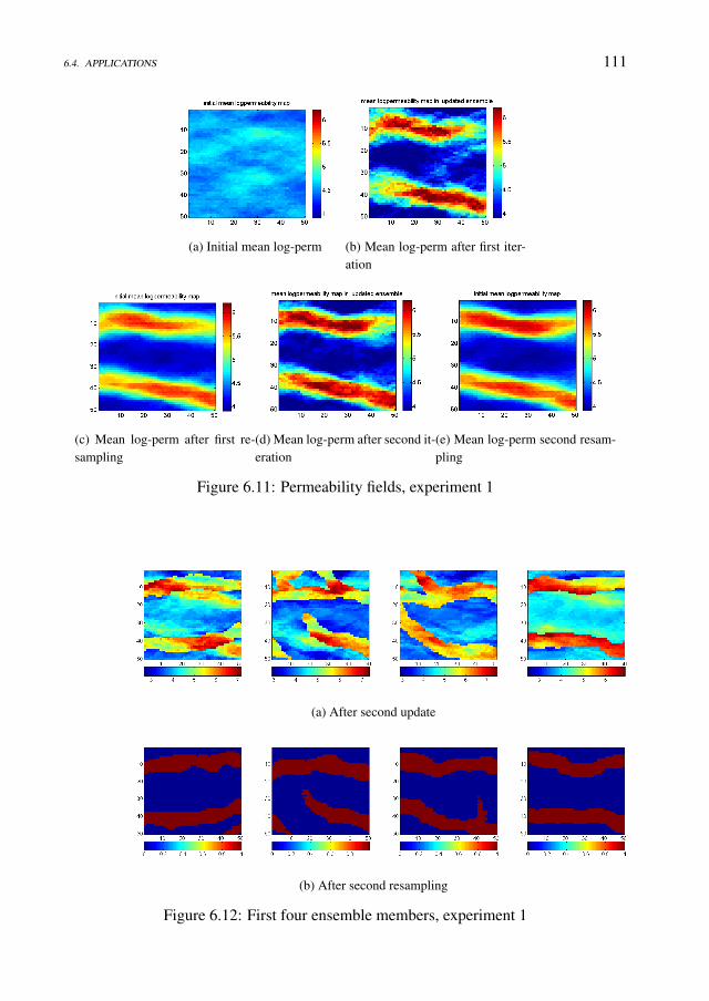
6.4. APPLICATIONS 111
(a) Initial mean log-perm (b) Mean log-perm after first iter-ation
(c) Mean log-perm after first re-sampling
(d) Mean log-perm after second it-eration
(e) Mean log-perm second resam-pling
Figure 6.11: Permeability fields, experiment 1
(a) After second update
(b) After second resampling
Figure 6.12: First four ensemble members, experiment 1
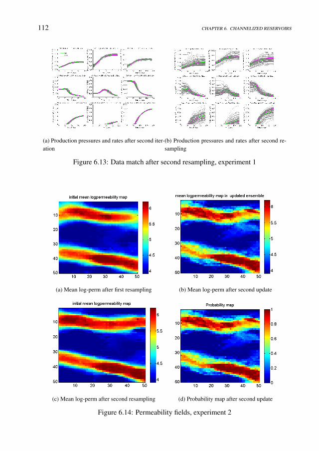
112 CHAPTER 6. CHANNELIZED RESERVOIRS
(a) Production pressures and rates after second iter-ation
(b) Production pressures and rates after second re-sampling
Figure 6.13: Data match after second resampling, experiment 1
(a) Mean log-perm after first resampling (b) Mean log-perm after second update
(c) Mean log-perm after second resampling (d) Probability map after second update
Figure 6.14: Permeability fields, experiment 2
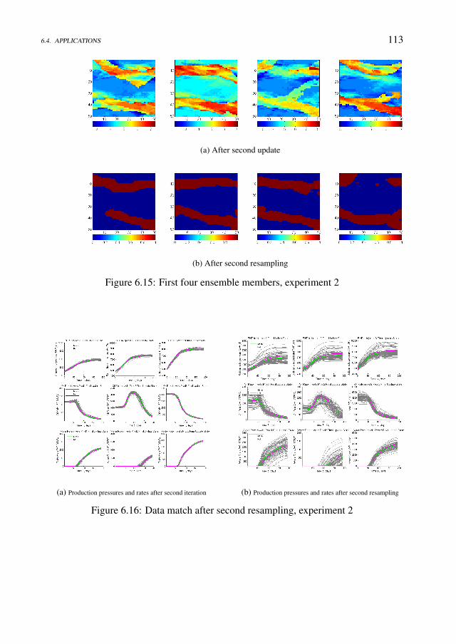
6.4. APPLICATIONS 113
(a) After second update
(b) After second resampling
Figure 6.15: First four ensemble members, experiment 2
(a) Production pressures and rates after second iteration (b) Production pressures and rates after second resampling
Figure 6.16: Data match after second resampling, experiment 2
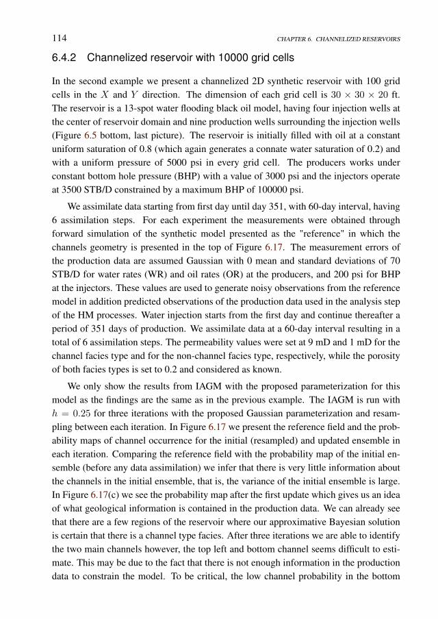
114 CHAPTER 6. CHANNELIZED RESERVOIRS
6.4.2 Channelized reservoir with 10000 grid cells
In the second example we present a channelized 2D synthetic reservoir with 100 gridcells in the X and Y direction. The dimension of each grid cell is 30 × 30 × 20 ft.The reservoir is a 13-spot water flooding black oil model, having four injection wells atthe center of reservoir domain and nine production wells surrounding the injection wells(Figure 6.5 bottom, last picture). The reservoir is initially filled with oil at a constantuniform saturation of 0.8 (which again generates a connate water saturation of 0.2) andwith a uniform pressure of 5000 psi in every grid cell. The producers works underconstant bottom hole pressure (BHP) with a value of 3000 psi and the injectors operateat 3500 STB/D constrained by a maximum BHP of 100000 psi.
We assimilate data starting from first day until day 351, with 60-day interval, having6 assimilation steps. For each experiment the measurements were obtained throughforward simulation of the synthetic model presented as the "reference" in which thechannels geometry is presented in the top of Figure 6.17. The measurement errors ofthe production data are assumed Gaussian with 0 mean and standard deviations of 70STB/D for water rates (WR) and oil rates (OR) at the producers, and 200 psi for BHPat the injectors. These values are used to generate noisy observations from the referencemodel in addition predicted observations of the production data used in the analysis stepof the HM processes. Water injection starts from the first day and continue thereafter aperiod of 351 days of production. We assimilate data at a 60-day interval resulting in atotal of 6 assimilation steps. The permeability values were set at 9 mD and 1 mD for thechannel facies type and for the non-channel facies type, respectively, while the porosityof both facies types is set to 0.2 and considered as known.
We only show the results from IAGM with the proposed parameterization for thismodel as the findings are the same as in the previous example. The IAGM is run withh = 0.25 for three iterations with the proposed Gaussian parameterization and resam-pling between each iteration. In Figure 6.17 we present the reference field and the prob-ability maps of channel occurrence for the initial (resampled) and updated ensemble ineach iteration. Comparing the reference field with the probability map of the initial en-semble (before any data assimilation) we infer that there is very little information aboutthe channels in the initial ensemble, that is, the variance of the initial ensemble is large.In Figure 6.17(c) we see the probability map after the first update which gives us an ideaof what geological information is contained in the production data. We can already seethat there are a few regions of the reservoir where our approximative Bayesian solutionis certain that there is a channel type facies. After three iterations we are able to identifythe two main channels however, the top left and bottom channel seems difficult to esti-mate. This may be due to the fact that there is not enough information in the productiondata to constrain the model. To be critical, the low channel probability in the bottom
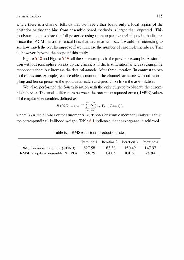
6.4. APPLICATIONS 115
where there is a channel tells us that we have either found only a local region of theposterior or that the bias from ensemble based methods is larger than expected. Thismotivates us to explore the full posterior using more expensive techniques in the future.Since the IAGM has a theoretical bias that decrease with ne, it would be interesting tosee how much the results improve if we increase the number of ensemble members. Thatis, however, beyond the scope of this study.
Figure 6.18 and Figure 6.19 tell the same story as in the previous example. Assimila-tion without resampling breaks up the channels in the first iteration whereas resamplingreconnects them but increase the data mismatch. After three iteration (in contrast to twoin the previous example) we are able to maintain the channel structure without resam-pling and hence preserve the good data match and prediction from the assimilation.
We, also, performed the fourth iteration with the only purpose to observe the ensem-ble behavior. The small differences between the root mean squared error (RMSE) valuesof the updated ensembles defined as
RMSE2 = (nd)−1
ne∑i=1
nd∑j=1
wi(Yj − Gj(xi))2,
where nd is the number of measurements, xi denotes ensemble member number i andwithe corresponding likelihood weight. Table 6.1 indicates that convergence is achieved.
Table 6.1: RMSE for total production rates
Iteration 1 Iteration 2 Iteration 3 Iteration 4
RMSE in initial ensemble (STB/D) 827.58 183.58 150.49 147.97RMSE in updated ensemble (STB/D) 158.75 104.05 101.67 98.94
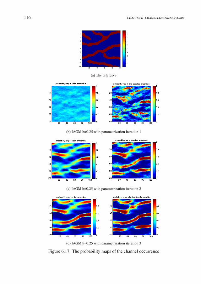
116 CHAPTER 6. CHANNELIZED RESERVOIRS
(a) The reference
(b) IAGM h=0.25 with parametrization iteration 1
(c) IAGM h=0.25 with parametrization iteration 2
(d) IAGM h=0.25 with parametrization iteration 3
Figure 6.17: The probability maps of the channel occurrence
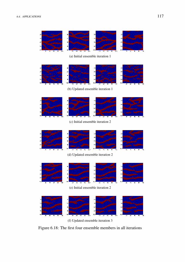
6.4. APPLICATIONS 117
(a) Initial ensemble iteration 1
(b) Updated ensemble iteration 1
(c) Initial ensemble iteration 2
(d) Updated ensemble iteration 2
(e) Initial ensemble iteration 2
(f) Updated ensemble iteration 3
Figure 6.18: The first four ensemble members in all iterations
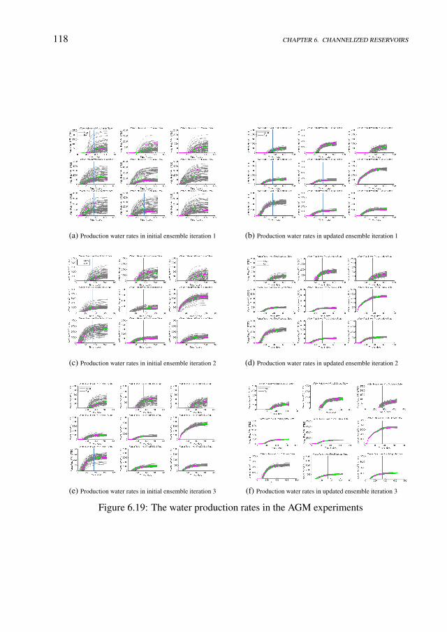
118 CHAPTER 6. CHANNELIZED RESERVOIRS
(a) Production water rates in initial ensemble iteration 1 (b) Production water rates in updated ensemble iteration 1
(c) Production water rates in initial ensemble iteration 2 (d) Production water rates in updated ensemble iteration 2
(e) Production water rates in initial ensemble iteration 3 (f) Production water rates in updated ensemble iteration 3
Figure 6.19: The water production rates in the AGM experiments

Chapter 7
Realistic facies simulation with theAPS model for a North Sea fieldcase
7.1 Introduction
In reservoir characterization, modern reservoir modeling and history matching aim atdelivering integrated models with quantified uncertainty, constrained on all availabledata. The "holy grail" of model updating/conditioning in the framework of Assisted His-tory Matching(AHM) is to obtain models which: match the past data within the modeland measurements uncertainties; incorporate all types of information (different measure-ments types) and preserve geological realism (consistent with the initial geo-model).The Fast-Model-Update workflow (FMU) resolves all of the above mentioned require-ments by handling reservoir models in the big-loop model updating framework and itprovides: a) a model chain, from depth conversion to simulation model, that is repeat-able and updatable; b) an ensemble framework for representation and prediction of un-certainty: c) ensemble methods for conditioning the model chain on dynamic data. Themajor principle of the FMU workflow is an automation and integration of all the mod-eling steps such that the whole model chain from depth conversion to simulation can berun in batch.In the implementation of any AHM process, one of the most important things to addressis the reservoir geological structure. When referring to geological structure we think of
This chapter is based on an article presented at 76th EAGE Conference and Exhibition, AmsterdamJune 16-19, 2014 where the coauthors are R.G. Hanea, T. Ek, J. Saetrom and D.B. Sollien
119

120 CHAPTER 7. REALISTIC UPDATES
faults position and top/base surfaces of the geological layers. The solution of integratingstructural uncertainties in the big loop approach was given by Seiler et al., 2010. Thenatural transition from structural geological uncertainties towards the rock and fluid un-certainties is represented by the facies distribution.In this study we apply a facies modeling process that can be used in an integrated mod-eling workflow (FMU). Therefore, we should ensure the flexibility, efficiency and ge-ologically realism of the process. In our opinion from a range of possible options (e.gmultipoint geostastatitics, level set, object and process based methods) the "low hangingfruit" methodology that fits our requirements is the plurigaussian concept (Sebacher etal., 2013). By using this concept, we generate possible facies realizations (distributions)in the reservoir domain.These facies instances must be consistent with the prior knowledge about the reservoirgeology (the number of the facies types, the possible transition between facies types, thedirection of the facies, the geometry of the facies, etc.) and honor the hard data (well logdata) and the sand probability cubes (derived from seismic data). The solution appliedhere is the adaptive plurigaussian simulation (APS) approach. The APS model con-sists of generating facies distributions conditioned to prior facies probability occurrencemaps. It is still part of the boarder truncated plurigaussian simulation (TPS) technique,using truncation maps, not in the multi-dimensional (usually bi-dimensional) space ofGRF, but in a multi-dimensional probability space.In a broader view we are interested in quantifying and reducing the uncertainties in thefacies distributions in a multiple realizations world. Therefore, the proposed processshould be updateable/conditioned based on all the available data by an ensemble basedmethod/tool.If until now the APS technology was applied with great success for synthetic cases rang-ing different depositional environments (See Sebacher et al, 2013, 2014), this is the firstattempt when APS is implemented and applied for a real field case in the North Con-tinental Shelf (NCS). Due to confidentiality issues we can not use the real name of thefield, so for simplicity we will name it "Loki" field. The novelty of this work consistsof realistic facies simulations for a real field case, consistent with the hard and soft dataas well as with the geological concept. This simulation process is repeatable and auto-mated/assisted by being integrated in the FMU framework of the big loop conditioningphilosophy. We are proposing an integrated workflow for facies generation and esti-mation using a simulation model that is able to create a link between the mathematicaltheory and real world.
7.2. THE GEOLOGICAL SETUP 121
7.2 The geological setup
We apply the pluri-gaussian facies modelling approach to the specific geological settingsof the Loki field, located in the North Sea, offshore mid-Norway. The field consists ofmultiple westerly tilted blocks, bounded by faults of Devonian age generated during theopening of the North Viking Graben (Fossen et al., 2000), and later reactivated duringTriassic and essentially Jurassic period. In term of sedimentology, the Loki field con-sists of Triassic deposits of the typical "redbeds" fluvial sandstones of the Upper Lundeand Statfjord Formations. The Statfjord Formation is strictly speaking of Rhaetian andEarly Jurassic age, but commonly attached to Triassic deposits as it consists of genet-ically similar sediments, deposited in the same environment, with no major unconfor-mity in the stratigraphic sequence. During the Triassic period, the climate evolved fromarid to semi-arid continental conditions (Dore, 1992; Van Der Zwan and Spaak, 1992).The sedimentary structures consisted on terminal sections of alluvial fans (Tunbridge,1984) with ephemeral braided streams terminating in sheetfloods, muddy flood plain orephemeral lake. Episodic water flooding and collapsing of channel banks resulted in thedeposition of crevasse splays along the margins of the channel systems. As a result of thearid conditions, most of the sediments were trapped within the continental environment(Collinson, 1986), hence the high accumulation of continental sediments observed in theTriassic sediment record of the North Sea. In the Loki field, the two reservoir forma-tions consist of sandy fluvial deposits interbedded with floodplain mudstones, for a totalthickness of 1000 m. A vertical progression in the style of fluvial bodies has been earlyrecognized and extensively studied for integration in the geological model in an attemptto match production data. Depending on the relative sea level variations, channel stylevaries from proximal high energy braided channels located at the foothill of alluvial fans,to more distal sinuous fluvial channels in a floodplain environment. Fluvial channels aremigrating laterally, the extent of the lateral migration being dependent on the slope ofthe depositional paleotopography and the velocity of the current: at the foothill of al-luvial fans, braided channels are confined and the channel belts they form are limitedin term of width (approximately 1 to 2 km wide); in the floodplain, channel belts be-come wider (approximately 5 to 10 km wide) as the system is closer to the seafront, withchannels becoming more sinuous and meandering. The variations in the style of fluvialbodies are accompanied by variations of facies and net-to-gross, grain sizes and poros-ity, grain sorting and permeability. Subsequently, the reservoir formations have beensubdivided in a number of reservoir units displaying similar characteristics in terms ofchannel geometry to fit to the subsurface observations: orientation, sinuosity, dimensions(width, depth), and proportions over floodplain mudstones. Channel belts are typicallymodelled with stochastic modelling techniques, most commonly with object-based mod-elling which insures that the continuity and geometry of channels are preserved in the
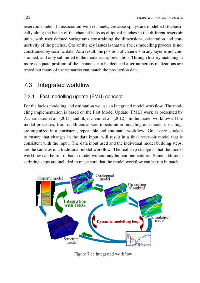
122 CHAPTER 7. REALISTIC UPDATES
reservoir model. In association with channels, crevasse splays are modelled stochasti-cally along the banks of the channel belts as elliptical patches in the different reservoirunits, with user defined variograms constraining the dimensions, orientation and con-nectivity of the patches. One of the key issues is that the facies modelling process is notconstrained by seismic data. As a result, the position of channels in any layer is not con-strained, and only submitted to the modeler’s appreciation. Through history matching, amore adequate position of the channels can be deduced after numerous realizations aretested but many of the scenarios can match the production data.
7.3 Integrated workflow
7.3.1 Fast modelling update (FMU) concept
For the facies modeling and estimation we use an integrated model workflow. The mod-eling implementation is based on the Fast Model Update (FMU) work as presented byZachariassen et al. (2011) and Skjervheim et al. (2012). In the model workflow all themodel processes, from depth conversion to saturation modeling and model upscaling,are organized in a consistent, repeatable and automatic workflow. Great care is takento ensure that changes in the data input, will result in a final reservoir model that isconsistent with the input. The data input used and the individual model building steps,are the same as in a traditional model workflow. The real step change is that the modelworkflow can be run in batch mode, without any human interactions. Some additionalscripting steps are included to make sure that the model workflow can be run in batch.
Figure 7.1: Integrated workflow
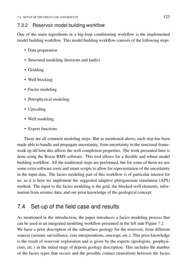
7.4. SET-UP OF THE FIELD CASE AND RESULTS 123
7.3.2 Reservoir model building workflow
One of the main ingredients in a big-loop conditioning workflow is the implementedmodel building workflow. This model building workflow consists of the following steps:
• Data preparation
• Structural modeling (horizons and faults)
• Gridding
• Well blocking
• Facies modeling
• Petrophysical modeling
• Upscaling
• Well modeling
• Export functions
These are all common modeling steps. But as mentioned above, each step has beenmade able to handle and propagate uncertainty, from uncertainty in the structural frame-work up till how this affects the well completion properties. The work presented here isdone using the Roxar RMS software. This tool allows for a flexible and robust modelbuilding workflow. All the traditional steps are performed, but for some of them we usesome extra software tools and smart scripts to allow for representation of the uncertaintyin the input data. The facies modeling part of this workflow is of particular interest forus, as it is here we implement the suggested adaptive plurigaussian simulation (APS)method. The input to the facies modeling is the grid, the blocked well elements, infor-mation from seismic data, and our prior knowledge of the geological concept.
7.4 Set-up of the field case and results
As mentioned in the introduction, the paper introduces a facies modeling process thatcan be used in an integrated modeling workflow presented in the left side Figure 7.2.We have a prior description of the subsurface geology for the reservoir, from differentsources (seismic surveillance, core interpretations, outcrops, etc.). This prior knowledgeis the result of reservoir exploration and is given by the experts (geologists, geophysi-cists, etc.) in the initial stage of deposit geology description. This includes the numberof the facies types that occurs and the possible contact (transition) between the facies
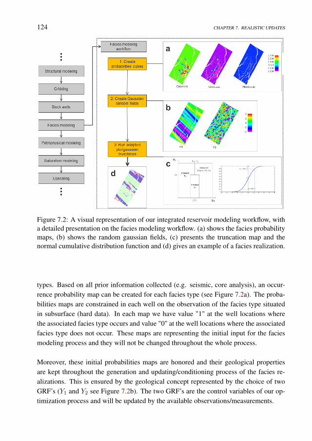
124 CHAPTER 7. REALISTIC UPDATES
Figure 7.2: A visual representation of our integrated reservoir modeling workflow, witha detailed presentation on the facies modeling workflow. (a) shows the facies probabilitymaps, (b) shows the random gaussian fields, (c) presents the truncation map and thenormal cumulative distribution function and (d) gives an example of a facies realization.
types. Based on all prior information collected (e.g. seismic, core analysis), an occur-rence probability map can be created for each facies type (see Figure 7.2a). The proba-bilities maps are constrained in each well on the observation of the facies type situatedin subsurface (hard data). In each map we have value "1" at the well locations wherethe associated facies type occurs and value "0" at the well locations where the associatedfacies type does not occur. These maps are representing the initial input for the faciesmodeling process and they will not be changed throughout the whole process.
Moreover, these initial probabilities maps are honored and their geological propertiesare kept throughout the generation and updating/conditioning process of the facies re-alizations. This is ensured by the geological concept represented by the choice of twoGRF’s (Y1 and Y2 see Figure 7.2b). The two GRF’s are the control variables of our op-timization process and will be updated by the available observations/measurements.
7.4. SET-UP OF THE FIELD CASE AND RESULTS 125
For each grid cell of the domain, we create a bi-dimensional map, like in left side ofFigure 7.2c. We define this map as the simulation map. In this quadratic domain, thetotal area is 1 and the area of the regions occupied by each facies type is equal withthe associated probabilities found in the maps provided by the experts. The distributionof the regions in the square allows modeling the contact between any two facies typeand the topological characteristics of the facies types. At the well locations, the mapconsists on a single square of surface 1, occupied by the facies type observed there.Consequently, there might be some parts of the reservoir domain where only two faciestypes occur (in terms of probabilities, only two probabilities are greater than zero). Inthis case, the map contains only two rectangular regions, each with area equals with theassociated probability of the facies type that occupies the region.Now, in each grid cell i, we need to simulate a facies type, conditioned to the probabil-ities given by the experts. For that, we apply the APS model. We generate samples forthe Gaussian fields Y1 and Y2 and assign the facies type depending on where the point(cdf(Y i
1 ), cdf(Y i2 )) falls in the simulation map built for the grid cell i. We generate an
ensemble of 100 realizations conditioned to the probability maps provided by the expertsand the probability maps calculated from the ensemble is consistent with the originals(Figure 7.3). In this manner we have defined an ensemble of facies maps realizations,conditioned to the probability maps provided by the geologists. These realizations de-pend only on the Gaussian fields used for simulations and are consistent with the faciesobservations at the well locations.After ensuring the above mentioned properties of the facies realization, another key is-sues in a multiple realizations world is the variability of the prior ensemble ensemble,which ensures that we are spanning the full uncertainty space (see Figure 7.4). Finally,the applicability and the success of the implementation of APS methodology for a realfield case is shown by the fact that the facies realization obtained were more consistentand closer with the geological concept and the hard and soft data than the ones obtainpreviously for the same field using different methodologies (indicator kriging). In theFigures 7.5, 7.6 and 7.7 realizations of facies maps obtained with the indicator krig-ing (bottom left) and with the APS (bottom right) are shown. At the top of the figureswe present the realizations of the Gaussian fields that provide the facies maps with theAPS methodology. A valuable prior information is related to the relative position ofthe crevasses (green) with respect to the floodplain (yellow) and the channel belt (red).The crevasses are encountered mainly on the border of the channel belt. With a visualinspection, one can observe that this restriction cannot be kept with the indicator krig-ing methodology, whereas the APS methodology was able to provide facies maps withplausible topology.
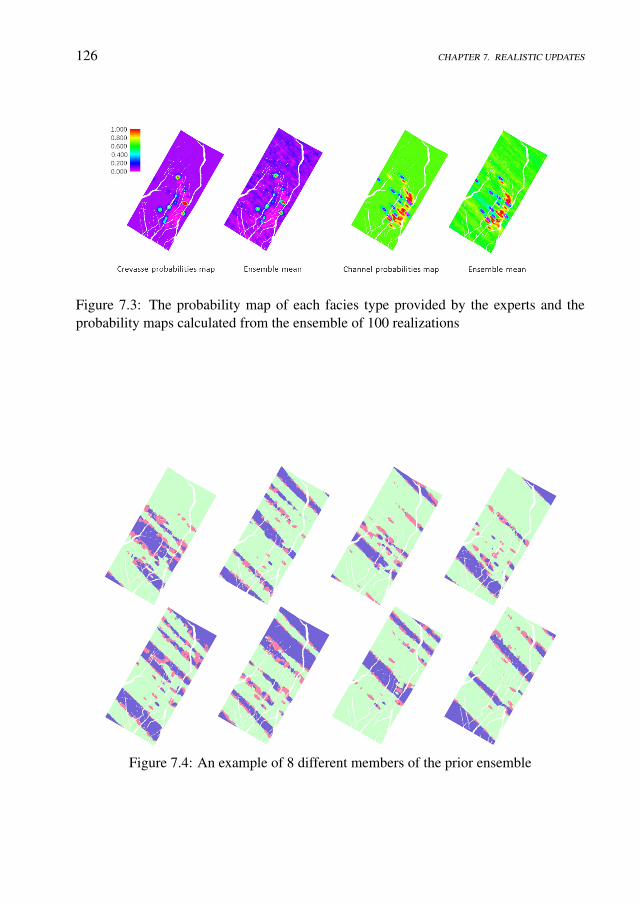
126 CHAPTER 7. REALISTIC UPDATES
Figure 7.3: The probability map of each facies type provided by the experts and theprobability maps calculated from the ensemble of 100 realizations
Figure 7.4: An example of 8 different members of the prior ensemble
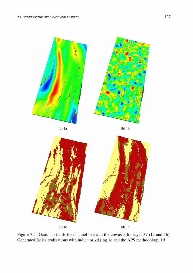
7.4. SET-UP OF THE FIELD CASE AND RESULTS 127
(a) 1a (b) 1b
(c) 1c (d) 1d
Figure 7.5: Gaussian fields for channel belt and the crevasse for layer 37 (1a and 1b);Generated facies realizations with indicator kriging 1c and the APS methodology 1d
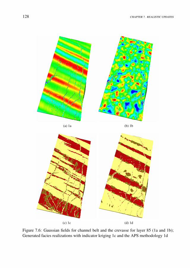
128 CHAPTER 7. REALISTIC UPDATES
(a) 1a (b) 1b
(c) 1c (d) 1d
Figure 7.6: Gaussian fields for channel belt and the crevasse for layer 85 (1a and 1b);Generated facies realizations with indicator kriging 1c and the APS methodology 1d
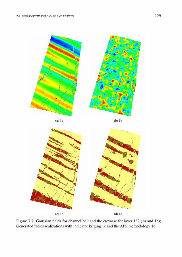
7.4. SET-UP OF THE FIELD CASE AND RESULTS 129
(a) 1a (b) 1b
(c) 1c (d) 1d
Figure 7.7: Gaussian fields for channel belt and the crevasse for layer 182 (1a and 1b);Generated facies realizations with indicator kriging 1c and the APS methodology 1d
Chapter 8
Conclusions
This research focussed on new parameterizations of facies fields, which are coupled withreliable AHM methods for geology estimation and uncertainty quantification. Two di-rections have been used for facies fields generation: the plurigaussian simulation model(TPS, Chapter 4, 5 and 7) and the multiple point geostatistical model (MPS, Chapter6). For the TPS model, the parameterization is straightforward with the Gaussian fieldsthemselves, for the MPS model a parameterization is not easy to define. The parame-terization proposed is carried out in a multidimensional Gaussian space by bridging theTPS methodology with the MPS.
8.1 Conclusions
• In Chapter 4 we presented a new approach of the facies estimation problem withEnKF, applied in the context of the truncated plurigaussian method. The trunca-tion map that is used for generation of the facies maps arises from a probabilisticapproach of the facies type fields. Actually, each probability can be viewed asa "distance" (to 0 or 1) that allows us to see how far we are to each facies type.This "distance" does not expresses a remoteness from a border (such as in thelevel set method) but shows the remoteness from two instances ("to be" whichis 1 and not "to be" which is 0). Starting with the assumption that the highest"distance" to 0 gives us the facies type in a certain location, we have built a ge-ological simulation model, which is further introduced in the EnKF context. Themodel is tested for the case with three facies types occurring, with the propertythat we could have transition between each two. The model is tested for differentgeostatistical properties of the Gaussian fields and different levels of uncertainty
130
8.1. CONCLUSIONS 131
introduced in generation of the model parameters. The novelty of the method hasthree directions.
– The first one is related to the truncation map. In the previous studies, wherethe truncation of two Gaussian fields has been made with a bidimensionalmap, it was constructed in an empirical manner and including the assignmentof each facies types in the demarcated areas generated by the intersectinglines of the map. The truncation map that appears in our study arises from theinternal construction of the model and also the assignment of the facies typein each zone of the map. The map depends only on two parameters which, ifchanged, perturb neither the geometry of the map, nor the assignment of thefacies types in the map zones. In addition, the parameters have the abilityto control the facies proportions. Consequently, the map parameters canbe introduced in the state vector for a better description of the uncertainty,improving in the estimation process.
– The second is related to the observation operator of the facies type at thewell locations. In the previous studies the facies observation operator is aproxy function which measures the affiliation of the pair of Gaussian fieldsto a specific area, in terms of yes or no. In our study we use an operatorthat measures the occurrence probability of each facies type. In this way wehave a multiple condition for the Gaussian fields, in the places where a faciestype occurs (the probability is 1) and in places where a facies type does notoccurs (the probability is 0). Consequently, our Gaussian field ensemble isnot conditioned to the map, but to the observations. From here arises thethird main difference.
– With the introduction of "the probabilities fields" in the context of the trun-cation plurigaussian approach, we have tried to explain how the Gaussianfields can be interpreted in the truncation simulation. In the past work theGaussian fields did not have a meaning, they were only useful for the faciesmaps generation. With this new approach, we gave a meaning to the Gaus-sian fields in the sense that their projection could be seen as probabilities. Asa consequence of the model (and hence, of the map), the probability mapsfor each facies type calculated from the facies field ensemble are consistentwith the ensemble averages of each probabilities fields (Figure 4.9)
At the end of the assimilation period, as result of the parameters estimation, we areable to offer a field, which we have named "estimated field", that is an estimatorof the truth field.
132 CHAPTER 8. CONCLUSIONS
• In the exploration phase a geological description of the subsurface is developedby the geologists and geophysicists. One important feature is represented by thefacies probability maps obtained based on all available information (well logs,seismic data etc.). In this study, we have introduced a methodology that relatesthe work developed in the exploration phase with the data assimilation process, asvaluable prior information.In Chapter 5, we have designed a geological simulation model in a plurigaussiansimulation context, which is able to sample facies maps from the prior proba-bility maps of the facies types. We named the geological simulation model theadaptive plurigaussian simulation (APS) model. The main differences with otherapproaches involving Gaussian fields truncation/simulation resides in the way inwhich the facies simulation/truncation maps are introduced and by the fact thatnot only a single map is used. In our approach, we do not construct a truncationmap in the Gaussian space, but for each grid cell, we construct a map in a domainof measure 1 of a metric space. We called this map the facies simulation map. Themap is based on the decomposition of the unitary domain in some zones assignedto the facies types of which areas must be equal to the probabilities found in themaps provided by the experts. The decomposition should be made in such a waythat the contact between the facies types and the topology of the facies field re-flect the reality. Therefore, a layout and a parametrization of the simulation mapis needed. Consequently, the core information collected at the wells, being incor-porated in the prior facies probability maps, will drive the simulation to alwaysprovide the correct facies type. This means that, throughout all the assimilationperiod, the facies types at the well location are not changed and satisfy the obser-vations and is not necessary to include extra procedures to reposition the faciestypes at the well locations, as in previous studies. To sample from the discretevariable named "facies type", of which distribution is known, we connect the uni-formly distributed variables with the Gaussian distributed variables through thenormal cumulative distribution function (cdf ) using the probability integral trans-form. Based on the cdf projection we have created spatially correlated fields withvalues in the [0,1] interval which at the starting point have uniform distribution.For that, at initial ensemble generation the Gaussian fields are generated uncorre-lated and unconstrained (stationary Gaussian random fields). This will ensure thatat each grid cell the facies type simulation will have the correct statistics at thebeginning of the data assimilation. At each grid cell, the facies simulation mapremains unchanged after each update being the object that relates the prior infor-mation provided by the experts with the plurigaussian simulation methodology.Basically, at the initial moment we simulate from the map with random variablesfrom uniform distribution on [0,1] and once the available measurements condition
8.1. CONCLUSIONS 133
the model parameters, we sample from the same map with random variables withvalues in [0,1] but not having the same uniform distribution. Keeping the simula-tion map (for each grid cell) throughout assimilation process means two importantthings related with the expert knowledge.
– Sampling from the same statistics at each moment but with variables (param-eters) at the beginning unconditioned and then conditioned to measurements(due the Bayesian inversion scheme)
– Keeping the topological request of the facies distribution.
An important novelty is the guiding direction that we constrain the EnKF to fol-low, introducing the facies observations as measurements at each assimilation timestep. This extra constraint does not reduce the variability in the updated ensembledrastically and only ensures that the ensemble goes in the right direction.
• In Chapter 6 we have presented a new parameterization of facies fields generatedusing multi point statistics (MPS). Since the truncated (pluri) Gaussian method iswell suited for facies updating with ensemble methods, but struggles with chan-nel structures (since the variogram has to be specified) we suggested estimating amarginal facies probability field from an ensemble generated using MPS, whichis well suited for channel type reservoirs, and parameterize this probability fieldwith a truncated marginally Gaussian field preserving the facies probabilities. Theadvantage is that the dependence structure is inherited from the training imageand do not have to be specified. Again we stress that prescribing an analyticalcovariance function that generates channels in combination with a truncation mapis (probably) an impossible task. Since the result is a truncated Gaussian field itis well suited for ensemble based methods and we are guaranteed that the updatedpermeability fields are facies fields without specifying a truncation. In addition,we combined the parameterization with the iterative adaptive Gaussian mixture(IAGM) filter for ensemble based Bayesian inversion. There were two main rea-sons for this. First, the IAGM is more suited for highly nonlinear problems thenthe EnKF, secondly, the IAGM has a resampling step which allowed us to use thealready existing technique of resampling from the training image using updatedprobability maps. However, since the IAGM can run assimilate all the data sev-eral times, there is no need for resampling after each update step and we only haveto perform resampling after each iteration (typically 2-4). We performed exper-iments on two channel type synthetic reservoirs and the conclusion drawn fromthe experiments were the same. The combination of the parameterization and theIAGM resulted in an advantage over existing methods in the sense that after a

134 CHAPTER 8. CONCLUSIONS
few iterations, the updated fields was able to keep the channel structure withoutperforming another resampling. Since the parameterization guarantees that theupdated fields are facies fields, the output of the algorithm was an ensemble ofchannelized reservoir models that had low data mismatch and good predictive ca-pabilities. If we had worked directly with log-permeability fields with we have tomake a compromise.
• In Chapter 7 we have presented a proof of concept for the APS methodology bysuccessfully implemented it and got very reliable results for a real field case inthe North Continental Shelf (NCS). We have obtained realistic facies simulationsfor a real field case, consistent with the hard and soft data as well as with thegeological concept. This simulation process is repeatable and automated/assistedby being integrated in the Fast Modeling Update (FMU) framework of the bigloop conditioning philosophy. We are proposing an integrated workflow for faciesgeneration and estimation using a simulation model that is able to create a linkbetween the mathematical theory and real world.
Bibliography
1. Aanonsen S. I., Naevdal G., Oliver D. S., Reynolds A. C., and B. Vall’es, TheEnsemble Kalman filter in reservoir engineering a review, SPE Journal, pp. 393-412, 2009.
2. Abrahamsen P., A review of Gaussian Random Fiedls and Correlation Functions,1997.
3. Agbalaka C. C., Oliver D. S., Application of the EnKF and localization to auto-matic history matching of facies distribution and production data, MathematicalGeosciences, 40, 353-374, 2008.
4. Agbalaka C. C., Oliver D. S., Automatic history matching of production and faciesdata with non-stationary proportions using EnKF, in SPE Reservoir SimulationSymposium, The Woodlands, Texas, USA, 2009.
5. Armstrong M., Galli A., Beucher H., Le Loc’h G., Renard D., Doligez B., EschardR. and Geffroy F., Plurigaussian Simulations in Geosciences. Springer BerlinHeidelberg, 2nd revised edition edition, 2011.
6. Arpat G., Caers J., A multi-scale pattern based approach to sequential simulation.Geostatistics Banff, Vol 1, pp 255-264, Springer, Dordrecht, 2004.
7. Avseth P., Mukerji T., Jorstad A., Mavko G., Veggeland T.: Seismic reservoirmapping from 3-D AVO in a North Sea turbidite system. Geophysics vol. 66. no.4, pp. 1157-1176, 2001.
8. Bengtsson T., Snyder C., Nychka D., Toward a nonlinear ensemble filter for high-dimensional systems. J. Geophys. Res., 108:35-45, 2003.
9. Bengtsson T., Bickel P., Li B., Curse-of-dimensionality revisited: Collapse of par-ticle filter in very large scale systems. Probability and Statistic, 2:316-334, 2008.
135
136 BIBLIOGRAPHY
10. Burgers G, van Leeuwen P. J., Evensen G., Analysis scheme in the ensembleKalman Filter. Mon Weather Rev 126, 1719-1724, 1998.
11. Caers J. and Zhang T., Multiple-point geostatistics: A quantitative vehicle for in-tegrating geologic analogs into multiple reservoir models. In: Grammer GM (ed)AAPG memoir,integration of outcrop and modern analogs in reservoir modeling:AAPG Memoir 80, p. 383-394, 2004.
12. Caers J. and Hoffman T., The probability perturbation method:a new look atBayesian inverse modeling. Math. Geol. 38, 81-100, 2006.
13. Casella G., Berger R. L., Statistical Inference, Duxbury, Thomson Learning, sec-ond edition, 2002.
14. Chang H., Zhang D. and Lu Z., History matching of facies distribution with theEnKF and level set parametrization, Journal of Computational Physics, 229(20),8011-8030, 2010.
15. Chen W. H., Gavalas G. R., Seinfeld J. H., and Wasserman M. L., A new algorithmfor automatic history matching. SPE Journal 14(4), 593-608, 1974.
16. Christoakos G., Random field models in earth sciences, Academic Press, NewYork, 1992.
17. Christoakos G., On the problem of permissible covariance and variogram models,J Water Resources Res 20, No 2, pp 251, Feb 1984.
18. Collinson J. D., Alluvial sediments. 20-61 in Sedimentary environments and fa-cies (second edition). Reading, H G (editor). (Oxford: Blackwell Scientific Pub-lications.) 1986.
19. Deutsch C. V., Journel A. G., GSLIB Geostatistical Software Library and User’sGuide,Applied Geostatistics Series, second ed., Oxford University Press, 1998.
20. Deutsch C. V. , Wang L., Hierarchical object-based modeling of fluvial reservoirs.Mathematical Geology 28, 857-880, 1996.
21. Dore A. G., Synoptic palaeogeography of the Northeast Atlantic Seaway: latePermian to Cretaceous. 421-446 in Basins on the Atlantic Seaboard: PetroleumGeology Sedimentology and Basin Evolution. Parnell, J (editor). SPeicla Publi-cation of the Geological Society of London, n. 62, 1992.
22. Doucet A., de Freitas N., Gordon N. (eds.): Sequential Monte-Carlo methods inpractice. Springer, New York, 2001.
137
23. Dovera L. and Della Rossa E., Multimodal ensemble Kalman filtering using Gaus-sian mixture models, Computational Geosciences, Volume 15, Issue 2, pp 307-323, 2011.
24. Evensen G., Sequential data assimilation with a non-linear quasigeostrophic modelusing Monte-Carlo methods to forecast error statistics. J. Geophys. Res. 99, pp143-162, 1994.
25. Evensen G., The Ensemble Kalman Filter: theoretical formulation and practicalimplementation. Ocean. Dyn. 53, pp 343-367, 2003.
26. Evensen G., Data Assimilation: The Ensemble Kalman Filter, Springer, 2006.
27. Fossen H., Odinsen T., Farseth R. B., and Gabrielsen T. H., Detachments and low-angle faults in the northern North Sea rift system. 105-131 in Dynamics of theNorwegian Margin. Nottvedt, A (editor). Special Publication of the GeologicalSociety of London, n. 167, 2000.
28. Galli A., Beucher H., Le Loc’h G., Doligez B., Heresim Group, The pros andcons of the truncated Gaussian method. In: Geostatistical simulations. KluwerAcademic, Dordrecht, pp 217-233, 1994.
29. Gao G., Gaoming L., Reynolds A. C., A Stochastic Optimization Algorithm forAutomatic History Matching, SPE Journal, Vol 12, Issue 2, pp 196-208, 2007.
30. Gaspari G. , Cohn, S. E., Construction of correlation functions in two and threedimensions. Q J R Meteor Soc 125,723-757, 1999.
31. Guardiano F., Srivastava M., Multivariate geostatistics:beyond bivariate moments.In: Geostatistics-Troia, vol1, pp. 133-144. Kluwer Academic, Dordrecht, Hol-land, 1993.
32. Hanea R. G., Ek T., Sebacher B., Saetrom J., Sollien D.B., Geologically RealisticFacies Updates for a North Sea Field, Extended abstract In Proceedings of the76th EAGE Conference and Exhibition, Amsterdam June 16-19, 2014
33. Honarkhah M., Caers J., Direct Pattern-Based Simulation of Non-stationary Geo-statistical Models, Math Geosci Volume 44, pp 651-672, 2012.
34. Hoteit I., Pham D. T., Korres G., Triantafyllou G., Particle Kalman filtering fordata assimilation in meteorology and oceanography. In 3rd WCRP InternationalConference on Reanalysis, pp.6, Tokyo, Japan, 2008a.
138 BIBLIOGRAPHY
35. Hoteit I., Pham D.T., Triantafyllou G., Korres G., A New approximative solutionof the optimal nonlinear filter for Data Assimilation in Meteorology and Oceanog-raphy. Mon. Wea. Rev., 136:317-334, 2008b.
36. Hu L. Y., Zhao Y., Liu Y., Scheepens C., and Bouchard A., Updating multi-point simulations using the ensemble Kalman filter. Computers and Geosciences,51(0):7-15, 2013.
37. Hu L.Y., Le Ravalec-Dupin M., An Improved Gradual Deformation Method forReconciling Random and Gradient Searches in Stochastic Optimizations, Mathe-matical Geology, Vol. 36, No. 6, 2004.
38. Hu L.Y., Liu Y., Scheepens C., Shultz A. W., Thompson R. D., Multiple-PointSimulation with an Existing Reservoir Model as Training Image, Math Geosci,Volume 46, Issue 2, pp 227-240, 2014.
39. Kelkar M. and Perez G., Applied Geostatistics for Reservoir Characterization:Society of Petroleum Engineers, 264 p., Richardson Texas, 2002.
40. Krishnan S., Boucher A. and Journel A. G., Evaluating information redundancythrough the tau model, in O. Leuangthong and C.V. Deutsch (eds.), GeostatisticsBanff Vol2, Springer, pp. 1037-1046, 2005.
41. Jafarpour B., Wavelet reconstruction of geologic facies from nonlinear dynamicflow measurements. IEEE Trans Geosci Remote Sens.doi:10.1109/TGRS.2010.2089464, 2010.
42. Jafarpour B., Khodabakhshi M., A probability conditioning method (PCM) fornonlinear flow data integration into multipoint statistical facies simulation. Math.Geosci. 43, 133-164, 2011.
43. Jafarpour B., McLaughlin D., Efficient permeability parametrization with discretecosine transform. In: The Proceedings of the SPE Reservoir Simulation Sympo-sium, Houston, TX, Paper SPE 106453, 2007.
44. Jafarpour B., Tarrahi M., Assessing the performance of the ensemble Kalman filterfor subsurface flow data integration under variogram uncertainty, Water ResourcesResearch, 47, W05537, 26 PP., 2011.
45. Jazwinski A., Stochastic processes and filtering theory. Academic Press, SanDiego, 1970.
46. Journel A. G., Combining knowledge from diverse data sources: An alternative totraditional data independence hypothesis: Math. Geol., v. 34, p. 573-596, 2002.
139
47. Journel A. G., Multiple-point Geostatistics: A state of the art. In Report 16, Stan-ford Center for Reservoir Forecasting, Stanford CA, 1993.
48. Lantuejoul C., Geostatistical simulation: models and algorithms. Spinger, Berlin,2002.
49. Lake L. W., Holstein E.D., Reservoir Engineering and Petrophysics-PetroleumEngineering Handbook, Vol V, Society of Petroleum Engineers, 2007
50. Le Loc’h G., Beucher H., Galli A., Doligez B., Heresim Group, Improvementin the truncated Gaussian method: combining several Gaussian functions. In:Proceedings of ECMOR IV: fourth European conference on the mathematics ofoil recovery, 1994.
51. Le Loc’h G., Galli A., Truncated plurigaussian method: theoretical and practicalpoints of view. In: Baafi EY, Schofield NA (eds) Geostatistics wollongong ’96,vol 1. Kluwer Academic, Dordrecht, pp 211-222, 1997.
52. Liu N. and Oliver D. S., Critical evaluation of the ensemble Kalman filter onhistory matching of geologic facies, SPE Reservoir Evaluation and Engineering,8(6), 470-477, 2005a.
53. Liu N. and Oliver D. S., Ensemble Kalman filter for automatic history matching ofgeologic facies, Journal of Petroleum Science and Engineering, 47(3-4), 147-161,2005b.
54. Lorentzen R. J., Flornes K. M., and Naevdal G., History matching channelizedreservoirs using the ensemble Kalman filter, SPE Journal, Vol 17, Issue 1, pp 137-151, 2012.
55. Lorentzen R. J., Naevdal G.,Shafieirad A., Estimating facies fields using the en-semble Kalman filter and distance functions, applied to shallow-marine environ-ments, SPE Journal, Vol 3, Issue 1, pp 146-158, 2012.
56. Mandel J., Beezley J. D., An ensemble Kalman-particle predictor-corrector filterfor non-Gaussian data assimilation. In ICCS 2009: Proceedings of the 9th Interna-tional Conference on Computational Science, pages 470-478, Berlin, Heidelberg,Springer-Verlag, 2009.
57. Massonnat G. J., Breaking of a Paradigm: Geology Can Provide 3D ComplexProbability Fields for Stochastic Facies Modelling. SPE Annual Technical Con-ference and Exhibition, Houston, Texas, 3-6 October, 1999.
140 BIBLIOGRAPHY
58. Matheron G., Beucher H., de Fouquet C., Galli A., Gue’rillot D., Ravenne C., Con-ditional simulation of the geometry of fluvio-deltaic reservoirs. SPE 1987 Annualtechnical conference and exhibition, Dallas, Texas, pp 591-599. SPE 16753, 1987.
59. Moreno D., Coupling Level Set Methods with the Ensemble Kalman Filter forConditioning Geological Facies Models to Well and Production Data, Ph.D. thesis,University of Bergen, Norway, 2009.
60. Oliver D. S., Moving averages for Gaussian simulation in two and three dimen-sions, Mathematical Geology, 27(8), 939-960, 1995.
61. Oliver D. S. and Chen Y., Recent progress on reservoir history matching: a review.Computational Geosciences 15(1), 185-221, 2011.
62. Oliver D. S., Reynolds A. J., Liu N., Inverse theory for petroleum reservoir char-acterization and history matching. Cambridge University Press, Cambridge, 2008.
63. Osher S., Fedkiw R., Level Set Methods and Dynamic Implicit Surfaces, Springer,2003.
64. Remy N., Boucher A., Wu J., Applied geostatistics with SGeMS a user’s guide,Cambridge University Press, 2009.
65. Roggero F., Hu L., Gradual deformation of continuous geostatistical models forhistory matching. SPE 49004, presented at the SPE annual technical conferenceand exhibition, New Orleans, LA, 27-30 September, 1998.
66. Sarma P., Durlofsky L., Aziz K., Kernel principal component analysis for efficient,differentiable parameterization of multipoint geostatistics. Math Geosci 40(1),3-32, 2008.
67. Sarma P., Chen W., Generalization of the Ensemble Kalman Filter using kernelsfor non-Gaussian Random Fields. In SPE Reservoir Simulation Symposium, TheWoodlands, Texax, February 2-4, 2009.
68. Sebacher B., Hanea R., Heemink A., A probabilistic parametrization for geolog-ical uncertainty estimation using the ensemble Kalman filter (EnKF), Computa-tional Geosciences, 2013, Volume 17, Issue 5, pp 813-832, 2013.
69. Sebastian Ng., Dahle Pg., Hauge R., Estimation of facies probabilities on theSnorre field using geostatistical AVA inversion. SEG Technical Program Ex-panded Abstracts 01/2008, 27(1), DOI:10.1190/1.3059282, 2008.
141
70. SGeMS The Stanford Geostatistical Modeling Software. http://sgems. source-forge. net/. Accessed 1 March 2012.
71. Stordal A., Karlsen H., Naevdal G., Skaug H. and Valles B. Bridging the ensembleKalman filter and particle filters. Computational Geosciences, 15(2), 293-305,2011.
72. Stordal A., Lorentzen R. J., An iterative version of the adaptive Gaussian mixturefilter. Computational Geosciences DOI 10.1007/s10596-014-9402-6, 2014.
73. Strebelle S., Conditional simulation of complex geological structures using multiple-point statistics. Mathematical Geology, vol 34, pp.1-22,2002.
74. Strebelle S., Zhang T., Non-Stationary multiple-point geostatistical models, In O.Leuangthong and C. V. Deutsch (eds.), Geostatistics Banff, pp. 235-244, 2005.
75. Skjervheim J. A., Evensen G., An Ensemble Smoother for Assisted History Match-ing, SPE Reservoir Simulation Symposium, 21-23 February, The Woodlands,Texas, USA, 2011.
76. Talagrand O., Courtier P., Variational assimilation of meteorological observationswith the adjoint vorticity equation. I: Theory. Quart. J. Roy. Meteor. Soc., 113,1311-1328, 1987.
77. Tunbridge I. P., Facies model for a sandy ephemeral stream and clay playa com-plex; the Middle Devonian Trentishoe Formation of North Devon, UK. Sedimen-tology, Vol. 31, 697-715, 1984.
78. Van den Zwan C. J., and Spaak P., Lower to Middle Triassic sequence stratigraphyand climatology of the Netherlands, a model. Palaeogeography, Palaeoclimatol-ogy, Palaeoecology, Vol. 91, 277-290, 1992.
79. Vasco D. W. and Datta-Gupta A., Integrating field production history in stochasticreservoir characterization. SPE Formation Evaluation 12(3), 149-156, (36567-PA), 1997.
80. Vasco D. W., S. Soon and A. Datta-Gupta, Integrating dynamic data into high-resolution reservoir models using streamline-based analytic sensitivity coefficients,SPE Journal 4(4), 389-399, 1999.
81. Xu C., Dowd P. A., Mardia K. V., Fowell R. J., A flexible true plurigaussian codefor spatial facies simulations. Computational Geosciences 32, 16291645, 2006.
142 BIBLIOGRAPHY
82. Zachariassen E., Skjervheim J.A., Vabo J. G., Lunt I., Hove J. and Evensen G.,Integrated Work Flow for Model Update Using Geophysical Monitoring Data,73rd EAGE Conference & Exhibition, Vienna, 2011.
83. Zafari M., Reynolds A.C., Assessing the Uncertainty in Reservoir Descriptionand Performance using the Ensemble Kalman filter. SPE Journal 12(3), 381:391,2007.
84. Zhang F. and Reynolds A. C., Optimization algorithms for automatic history match-ing of production data. In Proceeding of the 8th European Conference on theMathematics of Oil Recovery, Freiberg, Germany, 2002.
85. Zhang T., Journel A.G., Switzer P., Filter-based classification of training imagepatterns for spatial simulation, Mathematical Geology, Vol. 38(1), pp 63-80, 2006.
86. Zhao Y., Reynolds A. C., Li G., Generating facies maps by assimilating productiondata with EnKF paper spe113990. In:Proceedings of SPE/DOE symposium onimprovement oil recovery, Tulsa 20-23 April, 2008.
87. Zhou H., Li L., Gomez-Hernandez J. J., Hendricks Franssen H.J., Pattern Recog-nition in a Bimodal Aquifer Using the Normal-Score Ensemble Kalman Filter.Mathematical Geosciences, Vol. 44, 169:185, 2012.
Summary
An important key in reservoirs engineering is the development of reliable reservoir mod-els with high predictive capacity of production behavior in the existing and new drilledwells. The reservoir predictability is the starting point for guiding the production planto an optimum. In order to achieve this, the internal geological description of the reser-voir plays a crucial role. When referring to the internal geological description of thereservoir, one may think of a description of the spatial distribution of the petrophysicalproperties (permeability and/or porosity) or more natural, on a description of the spatialdistribution of the geological deposit formations (facies). The prior modeling of the fa-cies distribution is carried out using geostatistical tools in specialized modules, definingthus, the geological simulation model and its uncertainty. The choice of the geologicalsimulation model for facies field simulation takes into account the geological particular-ities of the reservoir. Irrespective of the geological simulation model used, the poorlyknowledge of geology leads to an initial reservoir model whose parameters are uncer-tain. This prior uncertainty is usually so large that the predictive capacity is limited. Toimprove the predictive capacity, the prior uncertainty is reduced in an Assisted HistoryMatching (AHM) process. To be able to couple the geological simulation model withan AHM method, a parameterization of the facies fields is needed. The research ob-jective of this thesis was to elaborate reliable parameterizations of the facies fields in asuch manner that, introduced in an AHM process, the updates to be able to: match thepast data within the model and measurement uncertainties; incorporate all types of infor-mation (different measurement types) and preserve the geological realism (consistencywith the initial geomodel). The research was oriented in two directions, depending onthe geological simulation model used.
In the context of truncated plurigaussian simulation model (TPS) two methodologieswere elaborated. The first methodology is tailored for cases where probability maps ofthe facies occurrence are not available, but only geometrical and topological informa-
143
144 SUMMARY
tion. In this case, we parameterized the binary field defined by each facies type with anew object denoted "the probabilities field". The probabilities fields are defined by pro-jection of Gaussian fields in [0,1] interval with a piece-wise linear projection function.We have created a geological simulation model, placed in the broader TPS methodol-ogy, with a truncation map not user defined but arising from the internal construction ofthe model. The AHM method used in this case is the Ensemble Kalman filter, condi-tioning the model parameters to production data (bottom hole pressures at the injectorsand oil and water rates at the producers) and hard data (facies observations at the welllocations). The conditioning on hard data was performed within an iterative process us-ing a probabilistic operator of the facies occurrence. In addition, is the first time whenthe parameters that define the truncation map are introduced in the estimation process,showing improvement in the uncertainty quantification of the facies distribution.
The second methodology is reserved for the case where probability maps of the fa-cies occurrence are available from a prior investigation carried out in the explorationphase of geology description. We introduced a geological simulation model for simula-tion of the facies fields so that the probability maps of the facies occurrence calculatedfrom an ensemble to be consistent with the given probability maps. The simulation isrealized at the grid cell level using uniform distributed variables, from a geometrical mapdesigned in an unitary domain. The map layout is chosen so that the simulated faciesfields obey to geometrical and topological requirements. The uniform variables used forfacies simulation are obtained by projection of Gaussian fields with the cumulative dis-tribution function. We called the geological simulation model the adaptive plurigaussiansimulation model (APS). We coupled the APS model with the EnKF obtaining updatesfor the facies probability maps together with an uncertainty quantification of the geol-ogy. The model parameters (the Gaussian fields) are constrained to production data andglobal facies proportions for a better quantification of uncertainty. The model was testedon two synthetic models with different complexity and one real field, reporting promis-ing results.
The second research direction refers to channelized reservoirs, modeled with a MPSgeological simulation models (SNESIM). We present a new parametrization of the faciesfields, which is further coupled with the iterative adaptive Gaussian mixture (IAGM) forhistory matching. The parameterization bridges ideas from MPS and TPS. The standardTPS parameterization ensures that the updated fields are facies fields, however, since thefield is jointly Gaussian it is not trivial to characterize channel type facies structures viaa covariance function (or variogram) in combination with a user defined truncation map.The MPS approach has the advantage of simulating channel type random fields, how-ever, they are discrete-valued and it is not trivial to connect this with ensemble based

145
inversion. We therefore suggest a combination of the two parameterizations. By es-timating marginal facies probabilities from a sample from MPS in combination with atraining image, we parameterize the marginal probability field with a (marginally) Gaus-sian random field where the truncation map is defined such that the integral for a faciestype in a given grid cell in the Gaussian domain coincides with marginal grid cell faciesprobability estimated from the ensemble. In addition, we combined the parameteriza-tion the iterative adaptive Gaussian mixture filter for ensemble based Bayesian inversion.There are two main reasons for this. First, the IAGM is more suited for highly nonlinearproblems then the EnKF, secondly, the IAGM has a resampling step which allowed us touse the already existing technique of resampling from the training image using updatedprobability maps.

Samenvatting
En belangrijke component in reservoir technologie is de ontwikkeling van betrouwbarereservoir modellen met een hoog voorspellend vermogen van het productie gedrag inbestaande en nieuw geboorde putten. De voorspelbaarheid van het reservoir is het uit-gangspunt voor een optimaal productie plan. De geologische beschrijving van het reser-voir speelt een cruciale rol om dit te bereiken. Bij een geologische beschrijving kan mendenken aan een omschrijving van de ruimtelijke verdeling van de petrofysische eigen-schappen (permeabiliteit en/of porositeit) of meer gangbaar, een omschrijving van deruimtelijke verdeling van de geologische afzettingen (facies). Het voorafgaande mod-elleren van de facies verdeling wordt gedaan in gespecialiseerde modellen met behulpvan geostatistische technieken, waardoor de onzekerheid van het geologisch simulatiemodel zodoende hier wordt gedefinieerd. In de keuze van het geologisch simulatiemodel voor simulatie van facies velden wordt rekening gehouden met de geologischebijzonderheden. Een slechte kennis van de geologie leidt, ongeacht welk geologischmodel wordt gebruikt, tot een reservoir model waarvan de parameters onzeker zijn. Dezevoorafgaande onzekerheid is normaal gesproken zo groot dat het voorspellend vermogenbeperkt is. Om het voorspellend vermogen te verbeteren wordt de voorafgaande onzek-erheid verminderd in een Assisted History Matching (AHM) proces. Daarvoor is eenparametrisering van facies velden noodzakelijk zodat het geologisch simulatie modelverbonden kan worden met een AHM methode. Het doel van dit proefschrift is om eenbetrouwbare parametrisering van facies velden te ontwikkelen zodat de updates, gein-troduceerd in het AHM proces, in staat zijn: de bestaande gegevens in het model ende meet onzekerheden te matchen; alle soorten van informatie the verenigen (verschil-lende type metingen) en geologisch realisme te behouden (in overeenstemming met hetoorspronkelijke geologisch model). Het onderzoek was georienteerd in twee richtingen,afhankelijk van het gebruikte geologisch simulatie model.
Twee methoden werden ontwikkelend in de context van afgeknotte meervoudigegaussische simulatie modellen (TPS). De eerste methodologie is gericht op gevallen
146

147
waar geen waarschijnlijkheidskaarten van facies voorkomen beschikbaar zijn, maar alleengeometrische en topologische informatie. In dit geval wordt het binaire veldgeparametriseerd en gedefinieerd door elk facies type met een nieuw object, aangeduidals "het waarschijnlijkheidsveld". Deze waarschijnlijkheidsvelden werden gedefinieerddoor een projectie van de gaussiche velden in een [0,1] interval met stuksgewijze lineaireprojectie functie. Een geologisch simulatie model is gecreeerd, geplaatst in breed TPSmodel, met een afgeknotte kaart niet gedefinieerd door de gebruiker, maar voortgekomenuit de interne constructie van het model. De AHM methode gebruikt in dit geval is deEnsemble Kalman filter (EnKF), waarin de parameters van het model worden gecon-ditioneerd aan productie data (onderste put druk van de injectoren en de olie en watersnelheden van de producenten) en harde gegevens (facies waarnemingen in de put). Deconditionering op harde data werd uitgevoerd door een iteratief proces met behulp vaneen waarschijnlijkheidsoperator van facies voorkomen. Het was ook de eerste keer datde parameters die de afgeknotte kaart definieren werden geintroduceerd in het schat-tingsproces en verbetering vertoonden in de onzekerheid kwantificering van de faciesdistributie.
De tweede methode is gericht op gevallen waar de waarschijnlijkheidskaarten van fa-cies voorkomen, verkregen uit een voorafgaand geologisch onderzoek, beschikbaar zijn.In deze methodiek werd een geologisch simulatie model geintroduceerd voor facies sim-ulatie velden waar de waarschijnlijkheidskaarten van facies voorkomen berekent van eenensemble in overeenstemming zijn met de voorafgaande waarschijnlijkheidskaarten. Desimulatie wordt gerealiseerd op grid cel niveau van een geometrische kaart ontworpenin een unitair domein met behulp van uniform verdeelde variabelen. De lay-out vande kaart is gekozen zodat de gesimuleerde facies velden voldoen aan de geometrischeen topologische voorwaarden. De uniforme variabelen gebruikt voor de facies simu-latie werden verkregen door een projectie van gaussische velden met een cumulatievedistributie functie. Wij noemen het geologische simulatie model het adaptieve meer-voudige gaussische simulatie model (APS). Het APS-model wordt gekoppeld aan EnKFverkregen actualisering voor de waarschijnlijkheidskaarten van facies voorkomen samenmet een onzekerheid kwantificering van de geologie. De model parameters (de gaus-sische velden) werden geconditioneerd aan productie gegevens en globale facies ver-houding voor een betere kwantificering van de onzekerheid. Het model werd getest optwee synthetische modellen met verschillende complexiteit en een daadwerkelijk veld,de uitkomsten toonde veelbelovende resultaten.
De tweede onderzoek richting concentreerde zich op gekanaliseerde reservoirs,gemodelleerd met MPS geologische simulatie modellen. Wij presenteren een nieuweparametrisatie van facies velden die worden gekoppeld aan de iteratieve adaptieve gaus-sische mix (IAGM) voor geschiedenis conditionering. De parametrisering overbrugtideeen van MPS en TPS. In de standaard TPS parametrisering zijn de facies velden de

148 SAMENVATTING
geactualiseerde velden, het veld is echter gedeeltelijk gaussisch waardoor het niet trivi-aal is om gekanaliseerde facies structuren te karakteriseren door een covariante functie(of variogram) in combinatie met een door de gebruiker gedefinieerde afgeknotte kaart.De MPS benadering heeft het voordeel van willekeurige veld simulatie van een kanaaltype, ze hebben een discrete waarde en het is niet triviaal om deze te verbinden met eenensemble gebaseerde inversie methode. Wij stellen daarom een combinatie van tweeparametrisaties voor. Door het schatten van de waarschijnlijkheid van marginale facies,van een monster van MPS in combinatie met een trainingsafbeelding, parametriseren wijde marginale waarschijnlijkheidsveld met een (marginale) willekeurig gaussisch veldwaar de afgeknotte kaart wordt gedefinieerd door de integraal van een facies type ineen bepaalde grid cel in het gaussische domein samenvalt met waarschijnlijkheid van demarginale grid cel facies die geschat wordt op basis van de ensemble. Daarnaast hebbenwij de parametrisering van de iteratieve adaptieve gaussische mix filter gecombineerdvoor een ensemble gebaseerde Bayesian inversie. Hiervoor zijn twee belangrijke rede-nen. Allereerst, de IAGM is meer geschikt dan EnKF voor zeer niet lineaire problemen,ten tweede, de IAGM heeft een herbemonsteringsstap die het toelaat om een trainingsaf-beelding te hermonsteren met behulp van geactualiseerde waarschijnlijkheidskaarten.

About the Author
Marius Bogdan Sebacher was born on 3th of August, 1975 in Bucharest, Romania. Hereceived the secondary education between 1989 and 1993 at Liceum "Alexandru IoanCuza" in Bucharest, Romania. From 1993 to 1997 he studied Mathematics at Universityof Bucharest, Faculty of Mathematics and Computer Science. In 1997 he started a Mas-ter of Science Program in Algebra at the same University and obtained the M.Sc. degreein noncommutative Algebra in 1999. From 1999 he started to teach Mathematics asassistant professor at Technical University of Civil Engineering in Bucharest, Romania.From 2010 until 2014 he continued the academic education in the group of Mathemati-cal Physics, Faculty of Electrical Engineering, Mathematics and Computer Science as aPh.D candidate, based on a research contract financed by the TNO, The Netherlands.
149