OF THE U.S. GEOLOGICAL SURVEY
132
JOURNAL OF OF THE U.S. GEOLOGICAL SURVEY SEPTEMBER-OCTOBER 1973 VOLUME 1, NUMBER 5 Scientific notes and summaries of investigations in geology, hydrology, and related fields U.S. DEPARTMENT OF THE INTERIOR
-
Upload
khangminh22 -
Category
Documents
-
view
1 -
download
0
Transcript of OF THE U.S. GEOLOGICAL SURVEY

JOURNAL OF
OF THE U.S. GEOLOGICAL SURVEY
SEPTEMBER-OCTOBER 1973 VOLUME 1, NUMBER 5
Scientific notes and summaries of investigations in geology, hydrology, and related fields
U.S. DEPARTMENT OF THE INTERIOR

UNITED STATES DEPARTMENT OF THE INTERIOR
ROGERS C. B. MORTON, Secretary
GEOLOGICAL SURVEY
V. E. McKelvey, Director
For sale by the Superintendent of Documents, U.S. Government Printing Office, Washington, D.C., 20402. Order by SD Catalog No. JRGS. Annual subscription rate, effective July 1,1973, $15.50 (plus $3.75 for foreign mailing). Single copy $2.75. Make checks or money orders payable to the Superin tendent of Documents.
Send all subscription inquiries and address changes to the Superin tendent of Documents at the above address.
Purchase orders should not be sent to the U.S. Geological Survey library.
Library of Congress Card No. 72-600241
The Journal of Research consists of six issues a year (January-February, March- April, May-June, July-August, September- October, November-December) published in Washington, D.C., by the U.S. Geological Survey. It contains papers by members of the Geological Survey on geologic, hydrol- ogic, topographic, and other scientific and technical subjects.
The Journal supersedes the short-papers chapters (B, C, and D) of the former Geological Survey Research ("Annual Re view") series of professional papers. The
synopsis chapter (A) of the former Geologi cal Survey Research series will be published as a separate professional paper each year.
Correspondence and inquiries concerning the Journal (other than subscription inquir ies and address changes) should be directed to the Managing Editor, Journal of Research, Publications Division, U.S. Geological Sur vey, Washington, D.C. 20244.
Papers for the Journal should be sub mitted through regular Division publication channels.
The Secretary of the Interior has determined that the publication of this periodical is necessary in the transaction of the public business required by law of this Department. Use of funds for printing this periodical has been approved by the Director of the Office of Management and Budget through February 11,1975.
HYDROL.Remote sensing of tur
bidity plumes in Lake ^Ontario. Page 609
Galkhaite, (Hg, Cu, Tl, Zn)(As. Sb) S 2 . from the/Getchell mine. Humboldt County, Nev. Page 515
H HYDRCi........
Aquifer diffusivity of trie OhioRiver alluvial', aquifer |by the
.. flo'od-wave response method.
Method for estimating the diver- sion potential opstr'eams in east- ern Massachusetts/and southern
PlibceneVnarine/fossils asot- Robles\For'mation, California ' '
HYDROL,^.Changes-in-fJo"ffafTbw^qharacter-
isiics of a\rectified\channel caused by vegetation, Jackson, Mjiss. Page 621
GEOL.An accurate Invar-wire extensometer. Page 569
GEOGRAPHIC INDEX TO ARTICLES[See Contents for articles concerning areas outside the United States and
articles without geographic orientation]

JOURNAL OF RESEARCHof the
U.S. Geological Survey
Vol. 1 No. 5 Sept.-Oct. 1973
CONTENTS
Abbreviations and symbols ................................................................... II
GEOLOGIC STUDIES
Permian paleogeography of the Arctic ................................ J. T. Dutro, Jr., and R. B. Saldukas 501Pliocene marine fossils in the Paso Robles Formation, California .......................................
.......................................................... W. 0. Addicott and J. S. Gatehouse 509Galkhaite, (Hg,Cu,Tl,Zn) (As,Sb)S2 , from the Getchell mine, Humboldt County, Nev. ......................
......................................... Theodore Botinelly, G. J. Neuerburg, and N. M. Conklin 515Disseminated pyrite in a latite porphyry at Texan Mountain, Hudspeth County, Tex. ............ T. E. Mullens 519Soda Creek springs Metamorphic waters in the eastern Alaska Range ...................................
............................................. D. H. Richter, R. A. Lamarre, and D. E. Donaldson 523The Dun Mountain ultramafic belt Permian oceanic crust and upper mantle in New Zealand ................
........................................................... M. C. Blake, Jr., and C. A. Landis 529A calorimetric determination of the standard enthalpies of formation of huntite, CaMg3 (C0 3 )4 , and artinite,
Mg2(OH)2 C0 3 '3H 2 0, and their standard Gibbsfree energies of formation;....................................................................................... B.S. Hemingway and R. A. Robie 535
The enthalpies of formation of nesquehonite, MgC0 3 '3H2 0, and hydromagnesite, 5MgO'4C0 2 5H 2 0 ....................................................................R. >1. Robie and B. S. Hemingway 543
Chemical analysis of rutile A pyrocatechol violet spectrophotometric procedure for the direct micro- determination of zirconium ................................................. Robert Meyrowitz 549
Spectrophotometric determination of tungsten in rocks by an isotope dilution procedure ................................................................................ E. G. Lillie and L. P. Greenland 555
Spectrochemical computer analysis Argon-oxygen d-c arc method for silicate rocks .............................................................................................. A. F. Dorrzapf, Jr. 559
Bathymetry of the continental margin off Liberia, West Africa ........................................................................................... J. M. Robb, John Schlee, and J. C. Behrendt 563
An accurate Invar-wire extensometer ................................. W. A. Duffield and R. 0. Burford 569Use of machine-processable field notes in a wilderness mapping project (Granite Fiords area), southeastern Alaska
................................................................ J.G. Smith and H. C. Berg 579Ice ages and the thermal equilibrium of the earth ........................................ D. P. Adam 587
HYDROLOGIC STUDIES
Aquifer diffusivity of the Ohio River alluvial aquifer by the flood-wave response method ................................................................................. H.F. Grubb and H. H. Zehner 597
A study of the distribution of polychlorinated biphenyls in the aquatic environment ..................................................................... H.J. Crump-Wiesner, H. R. Feltz, and M. L. Yates 603
Remote sensing of turbidity plumes in Lake Ontario ................................... E. J. Pluhowski 609Method for estimating the diversion potential of streams in eastern Massachusetts and southern Rhode Island.....
........................................................................... G.D. Tasker 615Changes in floodflow characteristics of a rectified channel caused by vegetation, Jackson, Miss. ...............
........................................................................... K. V. Wilson 621
Recent publications of the U.S. Geological Survey ...................................... Inside of back cover

II
[Singular and plural forms for abbreviations of units of measure are the same]
A ................ angstrom unitsA 3 ............... cubic angstromsa-c ............... alternating currentamp .............. amperesatm .............. atmospheresbbl ............... barrelsB.C. .............. Before ChristB.P. .............. Before Presentb.y. .............. billion yearsc ................. crystalline stateCx ............... molal concentration (of
substance x) cal ............... caloriescfs ............... cubic feet per secondCi ................ Curiescm ............... centimeterscm 2 .............. square centimeterscm 3 .............. cubic centimeterscpm .............. counts per minutecu ft .............. cubic feetcu mi ............. cubic milesd-c ............... direct currentemu .............. electromagnetic unitseV ............... electron voltsfpm .............. feet per minuteft ............ ....feetft 3 ............... cubic feetg ................. gramsgal ............... gallonsgpd ............... gallons per daygpm .............. gallons per minutehr ................ hoursHz ............... hertz (cycles per sec
ond) in. ............... incheskb ............... kilobarskg ................ kilogramskm ............... kilometerskm2 .............. square kilometerskm 3 .............. cubic kilometers-kV ............... kilovolts1 ................. liters
Ib ................ poundsIn ................ logarithm (natural)m ................ metersm ................ molal (concentration)m2 ............... square metersm 3 ............... cubic metersM ................ molar (concentration)me ............... milliequivalentsMeV .............. million electron voltsmg ............... milligramsmgd .............. million gallons per daymi2 .............. square milesmin ............... minutesml ............... millilitersmm .............. millimetersmol .............. molesmr ............... milliroentgensmV ............... millivoltsm.y. .............. million yearsM ................ micronsium ............... micrometersjumbo ............. micromhosn ................ neutronsN ................ normalng ................ nanogramsnm ............... nanometersOe ............... oerstedspCi ............... picocuriesP.d.t. ............. Pacific daylight timepH ............... pH (measure of hydro
gen ion activity) ppb .............. .parts per billionppm ............. .parts per millionrad ............... radiometricrpm .............. revolutions per minutesec ............... secondssq f t .............. square feetsq mi ............. square milesv ................. voltswt ............... weightyr ................ years

Jour. Research U.S. Geol. Survey Vol. 1, No. 5 , Sept.-Oct. 1973, p. 601 607
PERMIAN PALEOGEOGRAPHY OF THE ARCTIC
By J. THOMAS DUTRO, JR., and R. BIRUTE SALDUKAS, Washington, D.C.
Abstract. Three large land areas were dominant in the Arctic during the Permian: Fennoscandia, central and southern Siberia (Angara), and Canada. Smaller landmasses were in China, the Seward-Chukotskiy region, northern and eastern Siberia, and near Alaska. Coal deposits and strata bearing land plants covered a large area in central Siberia; saline basins containing red beds formed in the Zechstein, Perm, and West Texas basins as the seas withdrew, generally in the later Permian. Eugeosynclinal troughs, apparently limited to the Pacific border regions, were marked by volcanism and deposition of predominantly clastic sediments in many areas. Platform and miogeosynclinal deposits, dominated by carbonate rocks, preceded saline deposition in the basins and persisted on shallow shelves adjacent to the geosynclines. The Arctic Permian marine fauna evolved in middle Permian time because of partial isolation of the Arctic areas from the southern ocean. Endemism, latitudinal temperature controls, and the effect of ocean currents explain in large part the faunal patterns in Permian seas. Post-Permian tectonic movements account for anomalies in the present positions of some rock sequences and fossils. Northeasterly drift and counter clockwise rotation of the northern landmasses are suggested. Right- lateral shear along the southern edge of Asia is supported, followed by northward movement of peninsular India. -?;T
The Arctic seas in the Permian, particularly during the later Permian, harbored a marine invertebrate fauna that was impoverished as to variety of phyla and number of species. This Arctic Permian assemblage has been the subject of several comprehensive taxonomic papers since elements of the brachiopod fauna were first described by de Koninck (1847). Chief among these are Gobbett's (1963) description of brachiopods from Svalbard (Spitsbergen); Harker and Thor- steinsson's (1960) paper on the Permian of Grinnell Peninsula in the Canadian Arctic Islands;Dunbar's (1955) monograph of the central East Greenland brachiopods; Likharev and Einor's (.1.939) description of Novaya Zemlya faunas; Stepanov's (1936, 1937) papers on the Svalbard brachiopods; Zavo- dovskiy and others' (1970) atlas of northeastern U.S.S.R.; Stehli and Grant (1971) on Axel Heiberg Island; Grant's description of brachiopods from the Tahkandit Limestone, Alaska (in Brabb and Grant, 1971), and Waterhouse's descrip tion of brachiopods from the Yukon Territory (in Bamber and Waterhouse, 1971).
In attempting to understand the relationships of the Permian brachiopods in Arctic Alaska, Dutro (1961) proposed a
correlation of Arctic Permian strata and has continued to investigate the significance of these faunas in a paleo- geographic setting.
With the publication of the excellent paleotectonic maps of the Permian of the United States (McKee and others, 1967), followed by the magnificent Russian paleogeographical atlas (Nalivkin and Posner, 1969), much of the basic material for a more general synthesis of Permian paleogeography for the Northern Hemisphere became available.
We have prepared two paleogeographic maps (figs. 1, 2) on a polar projection which serve as a basis for interpretation of terrestrial and marine faunal and floral distributions at two time intervals during the Permian. The maps show the general distribution of land and sea and major lithofacies relative to present geography. They do not show the original positions of land and sea in the Permian or the relative amounts of different lithofacies or sources of clastic sediments; nor are they designed to depict drift, rotation, or other movement of continental masses (or plates), although some of these activi ties can be inferred (fig. 3).
Two segments of time were selected for the maps. Figure 1 depicts the Leonardian-Artinskian time and figure 2, Word- Kazanian time. Figure 1 was prepared to provide a basis for understanding the changes that occurred in the landscape during late Early Permian time. Figure 2 provides a geographic base for the biogeography shown in figure 3.
Figure 3 shows the distribution of selected elements of the biota for Word-Kazanian time. Generalized distributions of floras have been drawn from several sources but are chiefly modifications of syntheses by Andrews and Felix (1961) and by Radforth (1966). Vertebrate data were taken mostly from Olson's( 1962) work.
Two major elements of the marine fauna, brachiopods and verbeekinids, are depicted on figure 3. The brachiopods were analyzed by comparing the assemblage at various localities with that of Svalbard. Twenty-five species or species groups were selected as indicators of the Arctic Permian fauna. All of them occur in Svalbard. Using a modification of the Simpson coefficient technique (Simpson, 1960), other localities were found to include varying percentages of these indicators. The results have been plotted and contoured to give an impression of the degree of relatedness to Svalbard. Distribution of later
501

oi
o
to o O O o P3 I o
Figu
re 1
. Pal
eoge
ogra
phic
map
of
the
Nor
ther
n H
emis
pher
e du
ring
Leo
nard
ian-
Art
insk
ian
time.
Pol
ar p
roje
ctio
n, s
cale
app
roxi
mat
ely
1:67
,000
,000
at
lat
40°
N.

a c H
P3
O CO O
Figu
re 2
. Pal
eoge
ogra
phic
map
of
the
Nor
ther
n H
emis
pher
e du
ring
Wor
d-K
azan
ian
time.
Pol
ar p
roje
ctio
n, s
cale
app
roxi
mat
ely
1:67
,000
,000
at
lat
40°
N.
Ol
o CO

CA
THA
YSI
A
AN
GA
RA
li
NO
RT
H A
ME
RIC
A
ft A
. C
PEN
NO
SCA
ND
IA
Mix
ed A
ngar
an-C
atha
ysia
n fl
oras
A
ngar
an f
lora
M
ixed
Gon
dwan
an-C
atha
ysia
n fl
oras
Eur
-Am
eric
an f
lora
r S
^
/
SI
^ "
"
" n
Cat
hays
ian
flor
a D
irec
tion
of
post
-Per
mia
n m
ovem
ent
/
AFR
ICA
Isop
leth
of
Arc
tic
brac
hiop
od e
ndem
ism
G
ondw
anan
flo
ra
See
text
for
expl
anat
ion
Z
"O o
o
en
O
o £8 H
Figu
re 3
. Pal
eobi
ogeo
grap
hic
map
of
the
Nor
ther
n H
emis
pher
e du
ring
Wor
d-K
azan
ian
time.
Pol
ar p
roje
ctio
n, s
cale
app
roxi
mat
ely
1:67
,000
,000
at
lat
40°
N.
AH
, A
xel
Hei
berg
Isl
and;
E
, E
ngla
nd;E
G, E
ast G
reen
land
;EM
, E
dna
Mou
ntai
n F
orm
atio
n;G
, G
rinn
ell
Pen
insu
la;G
C,
Gra
nd C
anyo
n re
gion
;GE
, G
erst
er F
orm
atio
n; G
M,
Gla
ss M
ount
ains
;K,
Kan
in P
enin
sula
; K
O,
Kol
yma
basi
n; K
Z,
Kaz
an r
egio
n; M
, M
cClo
ud L
imes
tone
; M
A,
Man
kom
en F
orm
atio
n; M
O,
Mon
golia
; N
, N
uka
For
mat
ion;
NZ
, N
ovay
a Z
emly
a; 0
, O
rego
n; P
, P
olan
d; P
C,
Pai-
Cho
i R
ange
; PE
, Pe
chor
a ba
sin;
PH
, Ph
osph
oria
For
mat
ion;
S,
Sval
bard
; SA
, S
adle
roch
it F
orm
atio
n; S
E,
Sou
thea
st A
lask
a; S
R,
Salt
Ran
ge;S
W,
Sou
thw
est
Ala
ska;
T, T
aim
yr
Peni
nsul
a; T
A, T
ahka
ndit
Lim
esto
ne;
U,
Uss
uri
Val
ley;
V,
Ver
khoy
ansk
Ran
ge; Z
, Z
echs
tein
bas
in.

DUTRO AND SALDUKAS 505
Permian verbeekinid fusulinids (modified from Gobbett, 1967) shows a predominantly Tethyan pattern. Occurrences of these forms in western North America and the western Tethys area are attributed to distribution by currents from a possible center of dispersal in the east China-Japan region.
ANALYSIS OF RESULTS
Some of the major features of the Permian geography appear to be:1. In the Carboniferous and Early Permian, North America
and Laurasia were separated by a marine connection through the Russian Perm basin, which provided free exchange of marine faunas from the Tethys to the Arctic; in the latter part of the Permian, they were parts of a single large landmass.
2. The Perm basin was cut off from the Tethys by a land connection across its southern end during the late Early Permian (Kungurian).
3. Three major sites of evaporite and red bed deposition were the Perm, Zechstein, and West Texas basins.
4. Areas of coal swamp and coal deposits were the eastern United States (in the Early Permian), northern Siberia, and China.
5. A major volcanic region and, presumably, eugeosynclinal area bordered the ancient North Pacific. In the later Permian, the only connection between the world ocean and the Arctic basin was through straits between islands in the North Pacific.
THE ARCTIC PERMIAN MARINE FAUNA
The aspect of the Permian Arctic fauna that has intrigued paleontologists for a century is its domination by certain kinds of brachiopods and the virtual absence of other groups of animals. A few corals, bryozoans, and mollusks occur with the brachiopods; presence of echinoderm debris and sponge spicules indicates relative abundance of these phyla, but whole-body fossils are rare.
Among the brachiopods, a great many genera common in the tropical seas are absent; most of the assemblage can be accounted for in about 30 or 40 genera, and the characteristic forms number only about two dozen. The following species or species groups were selected for calculating the endemic ratios for the Arctic localities: Arctitreta kempei (Andersson), Derbyia cf. D. grandis Waagen, Anemonaria pseudohorrida (Wiman), Waagenoconcha irginae (Stuckenberg), Kochipro- ductus porrectus (Kutorga), Thamnosia arctica (Whitfield), Horridonia timanica (Toula), Globiella cf. G. simensis (Tschernyschew), Cancrinella spitzbergiana Gobbett, Ani- danthus aagardi (Toula), Kuvelousia weyprechti (Toula), Yakovlevia mammata (Keyserling), Lissochonetes spitz- bergianus (Toula), Chonetina superba Gobbett, Septacamera cf. S. kutorgae (Tschernyschew), Stenocisma spitzbergiana (Stepanov), Rhynchopora nikitini Tschernyschew, Neospirifer
striatoparadoxus (Toula), Licharewia spitzbergiana Gobbett, Pterospirifer alatus (Schlotheim), Spiriferella keilhavii (von Buch), Permophricadothyris asiatica (Chao), Martinia sp., Cleiothyridina royssiana (Keyserling), Pseudosyrinx wimani Gobbett, and Dielasmaplica (Kutorga).
Significant absentees from the Arctic assemblage are mem bers of the reef-associated productoid genera, including the leptodids, richthofenids, aulostegids, and scacchinellids. Also notable is the lack of diversity in the Arctic among the spiriferoids, rhynchonelloids, and terebratuloids that one finds at most tropical and subtropical localities. Stehli (1971) has analyzed the differences between Tethyan and Boreal brachio- pod facies at the family level and has concluded that the latter is completely dependent on cosmopolitan families. This reflects, in our view, an inheritance from the Carboniferous, early in the Permian when the Tethys was freely connected with the Arctic through a Uralian seaway.
At the species-group or species level, however, endemism developed in the Boreal region after the connection with the southern ocean was closed off late in the early part of the Permian. The calculated endemic ratios, showing relationships to the Svalbard fauna taken as unity, drop off regularly away from the Boreal region toward the presumed paleoequator (fig. 3). Approximately one-fifth of the taxa used in the analysis occur at most Tethyan stations, and this residue is considered to represent cosmopolitanism at the subgeneric level.
That apparent endemism and cosmpolitanism are inversely related when lower taxonomic levels are considered is not unexpected. In searching for an analog with which to compare the Boreal Permian brachiopod fauna, the molluscan distribu tion in restricted seas (Black Sea, Caspian Sea) comes first to mind. Runnegar and Newell (1971) have used these models to explain the Permian molluscan fauna of the Parana basin. It seems reasonable to assume that relatively rapid evolution of marine benthonic bivalved species would take place in a relict sea in which some abnormal environmental factors were present. In the Parana basin, Black Sea, and Caspian Sea this is probably low salinity. In the paleoarctic of the Permian, it was quite possibly related to temperature, although abnormal salinities may have been a factor in light of the formation of evaporite basins in several regions. Ustritskiy (1972) discussed the climate of the Permian and provided data that suggest that climatic gradients dispersed radially from a cold (glacial) area in north-central Siberia.
TERRESTRIAL FAUNA AND FLORA
Permian terrestrial vertebrates have been described from many places in the Northern Hemisphere, but mostly as isolated occurrences of limited faunas. One of the more comprehensive papers on these forms is Olson's (1962) analysis of north-central Texas and Uralian faunas. He con cluded that vertebrates evolved separately in the two regions throughout the Early Permian. In each instance, the pattern of

506 PERMIAN PALEOGEOGRAPHY OF THE ARCTIC
progression is from aquatic to upland forms. Interconnections were established by middle Permian time, however, and several migratory exchanges are postulated to account for relation ships between early Late Permian genera in Texas and their Kazanian counterparts in Russia.
Paleobotanists have long considered the Permian floras as constituting four distinct provinces: (1) Eur-American, (2) Angaran, (3) Cathaysian, and (4) Gondwanan (Andrews and Felix, 1961; Radforth, 1966). Distributions of these provinces show clearly the eastward advance of the Eur- American flora into central Asia after the establishment of the land connection across the southern U.S.S.R. Two areas of floral overlap are also indicated, one in China (Angaran- Cathaysian) and one in southeast Turkey (Gondwanan- Cathaysian, see Wagner, 1962). The Gondwanan flora, as such, is found in the Northern Hemisphere only in peninsular India.
BIOGEOGRAPHIC INTERPRETATIONS
Invertebrate faunas in the Arctic inherited their basic character from the late Carboniferous faunas, mainly because a marine connection existed from the southern seas through the Perm basin. This connection was cut off in the latter part of the Early Permian, and the younger Arctic Permian assemblage reflects endemism in the northern ocean (fig. 3).
Low correlations with Svalbard are of two kinds. The presence of only a few hardy species in the Zechstein and Perm embayments undoubtedly reflects rigorous environ mental conditions high salinity associated with the de velopment of evaporite basins. On the other hand, a regular decrease in correlation southward along the west side of North America and the east side of Asia possibly reflects some latitudinal, perhaps temperature, factor.
Conversely, the Eur-American flora and terrestrial verte brates evolved separately through the Early Permian but extended their ranges eastward across the land area that was formed in the southern U.S.S.R. toward the middle of the period.
Overlap of Angaran and Cathaysian floras is explained by proximity. Assumed paleowind directions would have assisted this mixing process. The seemingly anomalous flora in Turkey can be explained by large-scale tectonic activity since the Permian, as can the position of peninsular India.
TECTONIC IMPLICATIONS
The maps show rather clearly that the major land areas of the Northern Hemisphere during the middle and later Permian were part of a single large continent. The distribution of the Eur-American flora certainly implies that no Atlantic Ocean existed at that time. Land in the Southern Hemisphere seems to have been consolidated into a large but separate Gond wanan continent. A marine connection through southern Asia
and the Mediterranean (pre-Tethys) best accounts for faunal relationships in the Permian oceans.
A volcanic belt paralleling the present north Pacific coast probably was the site of eugeosynclincal deposition. Rather narrow continental shelves extended southward from Alaska toward both China and the southwestern United States.
Most recent analyses of evaporite deposition conclude that major basins formed within an area extending from about lat 30 N. to 30 S., in locations far south of the present positions of the West Texas, Zechstein, and Perm basins. Consequently, significant post-Permian plate movements must have taken place.
The northern continent may have started to break up by northeastward movement accompanied by counterclockwise rotation of the three core areas North America, Fenno- scandia, and Angara (see Briden, 1968). This movement need not have been uniform, and there is reason to believe that each block moved at a different rate. After the mid-Atlantic ridge area became active, perhaps in the Jurassic, North America could have begun its westward drift, a late phase of its counterclockwise movement.
In the tropical latitudes, floral distributions suggest that great lateral motions took place. The presence of the mixed Gondwanan-Cathaysian flora in Turkey can be explained by westward shift through nearly 40° of longitude. This is about the amount of lateral shear postulated on geomagnetic grounds by Irving (1967).
A later movement of India northward from Gondwana would account for its anomalous present position both geologically and biogeographically (fig. 3). The peculiar attenuated peninsulas and islands in what is now the Himalaya region also seem to reflect this northward drift.
REFERENCES CITED
Andrews, H. N., Jr., and Felix, C. I., 1961, Studies in paleobotany:New York, John Wiley and Sons, 487 p.
Bamber, E. W., and Waterhouse, J. B., 1971, Carboniferous andPermian stratigraphy and paleontology, northern Yukon Territory,Canada: Bull. Canadian Petroleum Geology, v. 19, no. 1, p. 29 250,27 pis., 19 figs.
Brabb, E. E., and Grant, R. E., 1971, Stratigraphy and paleontology ofthe revised type section for the Tahkandit Limestone (Permian) ineast-central Alaska: U.S. Geol. Survey Prof. Paper 703, 26 p., 2 pis.,11 figs. .
Briden, J. C., 1968, Paleoclimatic evidence of a geocentric axial dipolefield, in Phinney, R. A., ed., The history of the earth's crust, asymposium: Princeton, N.J., Princeton Univ. Press, p. 178 194.
Dunbar, C. 0., 1955, Permian brachiopod faunas of central EastGreenland: Medd. Grdnland, v. 110, no. 3,169 p., 32 pis.
Dutro, J. T., Jr., 1961, Correlation of the Arctic Permian: Art. 231 inU.S. Geol. Survey Prof. Paper 424-C, p. C225-C228.
Gobbett, D. J., 1963, Carboniferous and Permian brachiopods ofSvalbard: Norsk Polarinst. Skr., no. 127, 201 p., 25 pis.
1967, Palaeozoogeography of the Verbeekinidae (PermianForaminifera), in Adams, C. G., and Ager, D. V., eds., Aspects ofTethyan biogeography a symposium: Systematics Assoc. Pub. 7, p.77-91.

DUTRO AND SALDUKAS 507
Marker, Peter, and Thorsteinsson, Raymond, 1960, Permian rocks and faunas of Grinnell Peninsula, Arctic Archipelago: Canada Geol. Survey Mem. 309,146 p.
Irving, E., 1967, Paleomagnetic evidence for shear along the Tethys,in Adams, G. C., and Ager, D. V., eds., Aspects of Tethyan biogeo- graphy a symposium: Systematics Assoc. Pub. 7, p. 59 76.
Koninck, L. de, 1847, Recherches sur les animaux fossiles Pt. 1. Monographic des genres Productus et Chonetes: Lie'ge, H. Dessain, 246 p., 20 pis.
Likharev, B. K., and Einor, 0. L., 1939, [Paleontology of the Soviet Arctic, Pt. IV; Contributions to the knowledge of the upper Palaeozoic fauna of Novaya Zemlya, Brachiopoda]: Arctic Institute [U.S.S.R.] Trans., v. 127, 245 p., 28 pis. [In Russian].
McKee, E. D., Oriel, S. S., and others, 1967, Paleotectonic maps of the Permian System: U.S. Geol. Survey Misc. Geol. Inv. Map. 1-450,164 p., 20 pis., 12 figs.
Nalivkin, V. D., and Posner, V. M., eds., 1969, Devonskiy, Kamen- nougol'nyy i Permskiy periody [Devonian, Carboniferous, and Permian], v. 2 of Vinogradov, A. P., ed.-in-chief, Atlas litologo- paleogeographeskikh kart SSSR [Atlas of lithological-paleogeo- graphical maps of the U.S.S.R.]: Moscow, Ministerstvo Geologii- Akad. Nauk SSSR, 65 pis.
Olson, E. C., 1962, Late Permian terrestrial vertebrates, U.S.A. andU.S.S.R.: Am. Philos. Soc. Trans., 1962, v. 52, pt. 2, 224 p.
Radforth, N. W., 1966, The ancient flora and continental drift, inGarland, G. D., ed., Continental drift: Royal Soc. Canada Spec. Pub.9, p. 53-70.
Runnegar, Bruce, and Newell, N. D., 1971, Caspian-like relict molluscanfauna in the South American Permian: Am. Mus. Nat. History Bull.,v. 146, art. 1,66 p.
Simpson, G. G., 1960, Notes on the measurement of faunal resem blance: Am. Jour. Sci. (Bradley Volume), v. 258-A, p. 300-311.
Stehli, F. G., 1971, Tethyan and Boreal Permian faunas and their significance, in Dutro, J. T., Jr., ed., Paleozoic perspectives; A paleontological tribute to G. Arthur Cooper: Smithsonian Contr. Paleobiology 3, p. 337-345, 6 figs.
Stehli, F. G., and Grant, R. E., 1971, Permian brachiopods from Axel Heiberg Island, Canada, and an index of sampling efficiency: Jour. Paleontology, v. 45, no. 4, p. 502-521, pis. 61-66, 4 figs
Stepanov, D. L., 1936, [Contribution to the knowledge of the brachiopod fauna of the upper Paleozoic of Spitzbergen]: Lenin grad Bubnoff State Univ. Ann., no. 9, Geol. iss., 2, p. 114-128, pis. 1 5 [In Russian].
1937, [Permian brachiopods of Spitzbergen]: Arctic Inst.[U.S.S.R.] Trans., v. 76, p. 105-192, pis. 1-9 [In Russian].
Ustritskiy, V. I., 1972, The.Permian climate (a comparison of paleo- biogeographic and paleomagnetic data): Internat. Geology Rev., v. 14, no. 12, p. 1279-1286, 4 figs., table. Originally pub. as: Klimat permi (sopostavleniye paleobiogeograficheskikh i paleomagnitnykh dannykh): Akad. Nauk SSSR Izvest., Ser. Geol., 1972, no. 4, p. 3-12, 4 figs.
Wagner, R. H., 1962, On a mixed Cathaysia and Gondwana flora from SE Anatolia (Turkey): Cong. Avancement Etudes Stratigraphie et Geologic Carbonifere, 4th, Heerlen, 1958, Compte rendu, v. 3, p. 745-752, pis. 24-28.
Zavodovskiy, V. M. and others, 1970, [Field atlas Permian fauna and flora of northeastern U.S.S.R.]: Magadan, Ministry Geology, RSFSR, 407 p., 101 pis. [In Russian].


Jour. Research U.S. Geol. Survey Vol. l,No.5,Sept.-Oct. 1973, p. 509 514
PLIOCENE MARINE FOSSILS IN THE PASO ROBLES FORMATION, CALIFORNIA
By WARREN O. ADDICOTT and JON S. GALEHOUSE,1
Menlo Park, Calif., San Francisco, Calif.
Abstract. Marine invertebrates from the Paso Robles Formation recently discovered near Atascadero, Calif., indicate that the basal part of this chiefly nonmarine deposit is of provincial early Pliocene age. Heretofore the lack of direct fossil or radiometric evidence of the age of the Paso Robles has made it a difficult unit to place in the late Cenozoic history of the Coast Ranges. The assemblage is dominated by Ostrea vespertina and by Nettastomella rostrata, a rock-boring bivalve; its mode of preservation indicates that the fossils are in place and have not been recycled from older marine formations. This occurrence suggests that during the early Pliocene a seaway connected the present southern Salinas Valley area with the northern part of the Santa Maria basin; the fossils occur about halfway between the southernmost exposures of the Pancho Rico Formation near San Miguel and fossiliferous strata east of Pismo Beach, both marine units of early Pliocene age.
The Paso Robles Formation, as originally defined by Fairbanks (1898, 1904), crops out nearly continuously over approximately 1,000 sq mi of the upper Salinas Valley in the southern part of the California Coast Ranges (fig. 1). The formation is mainly a late Cenozoic continental deposit of gravel, sand, silt, and clay. In general, the coarser sand and gravel occur as stream-channel deposits, whereas the finer sand, silt, and clay occur as flood-plain deposits. The Paso Robles has long posed a problem in interpreting the late Cenozoic geologic history of the southern part of the California Coast Ranges because of the lack of direct fossil or radiometric evidence of its age (Galehouse, 1967). Previous age determinations have been based upon such indirect criteria as long-range correlations, stratigraphic relations, and concepts of late Cenozoic diastrophic history.
This report describes the first diagnostic fossils found in the Paso Robles Formation and interprets their age and paleo- graphic significance. It is of interest that they are of marine origin. An assemblage of oysters and other marine inverte brates was discovered in 1971 near the base of the Paso Robles Formation at a locality a few miles east of Atascadero, Calif., during a California State University stratigraphy class field trip led by Galehouse, who hereby thanks the participating students. The locality was subsequently revisited by the
1 California State University, Department of Geology.
authors and D. L. Durham; at that time most of the material described and illustrated in this report was collected.
Acknowledgments.-^!'e wish to acknowledge critical re views of the manuscript by D. L. Durham, E. W. Hart, and C. A. Repenning. Hart, of the California Division of Mines, kindly made available geologic mapping and stratigraphic data
123° 122' 120° 119°
TRANSVERSE RANGES
- 35°
34°
100 MILES
I 1 I0 100 KILOMETERS
Figure 1. Index map of central California, showing distribution of the Paso Robles Formation (from Galehouse, 1967).
509

510 PLIOCENE MARINE FOSSILS, PASO ROBLES FORMATION, CALIFORNIA
from his investigation of the Santa Margarita area. Fossil photography is by Kenji Sakamoto.
GEOLOGIC SETTING
The marine fossils discovered are exposed near the southern margin of an extensive area of Paso Robles terrane character istic of the upper Salinas Valley (fig. 2). The fossil locality (USGS M4621) is in a quarry along the south side of the Atascadero-Creston road about 2 miles east of Atascadero and nearly 3,000 feet due north of the southeast corner (lat 35° 30' N.; long 120°37.5' W.) of the Templeton, Calif., 71/2-minute quadrangle (U.S. Geol. Survey topographic map). The ex posure here is in the lowermost part of the Paso Robles
120° 45'
bs-Pliopedia Santa HfcjKlocality
Margarita
X M4621USGS marine
invertebrate locality
SMILES
5 KILOMETERS
Formation, which in this area unconformably overlies Monterey Shale (Jennings, 1958; Durham, 1973). Litholog- ically, the section exposed is typical of the Paso Robles Formation, consisting mainly of sand and gravel. The gravel clasts exposed in the quarry were derived from the Monterey Shale. The section exposed here differs from the Paso Robles Formation exposed elsewhere mainly in that it contains marine invertebrate fossils in place. The nonopaque heavy minerals, pebble lithology and imbrication, and foreset beds all indicate that the source area was to the south and southeast, the same as for the nonfossiliferous beds of the Paso Robles Formation in nearby outcrops. Much of the detritus probably was shed from the northern part of the La Panza Range (see Galehouse, 1967, for details).
PALEONTOLOGY
Faunal assemblage
Figure 2. Distribution of the Paso Robles Formation in the Atascadero-Santa Margarita area, central California, showing occurrences of marine fossils (after Jennings, 1958, and E. W. Hart, written commun., July 1972).
A small assemblage of epifaunal, boring, and nestling marine invertebrates, principally mollusks, has been identified from USGS Cenozoic locality M4621, and are listed here:
Marine invertebrates from the Paso Robles Formation
Pelecypods:Crassostrea titan (Conrad)(fig. 3a) [reworked]Hinnitesgiganteus (Gray)(fig. 3i, o)Nettastomella rostrata (Valenciennes) (fig. 3e, j)Ostrea atwoodi Gabb (fig. 3p, r)Ostrea vespertina Conrad (fig. 3a c, f, h, 1 n )Sphenia luticola (Valenciennes)
Barnacle:Balanus sp. (fig. 3#, i)
Brachiopod:Terebratalia cf. T. arnoldi Hertlein and Grant (fig. 3d, k)
By far the most abundant species is Ostrea vespertina Conrad. The lower valves of this small oyster are strongly plicate and are generally ovate falcate in outline; a few of the smaller valves are more ovate. In this collection upper valves of this species are more abundant than lower valves. They vary from smooth to undulate and none are as strongly plicate as the lower valves. The upper valves closely resemble the small form
of this species figured by Woodring, Stewart, and Richards (1940, pis. 8 and 10) as 0. vespertina sequens Arnold. Indeed, in the absence of lower valves, one would probably identify the upper valves as being of 0. vespertina forma sequens. Conversely, without the upper valves, the lower valves would be regarded as 0. vespertina s.s. The oyster is here identified as 0. vespertina in the context of variation described by Woodring (in Woodring and Bramlette, 1950) for specimens from the Santa Maria basin. Upper valves of some of the small specimens from the Santa Maria area were described as "being practically flat," the larger as being "moderately plicate to warped" (Woodring and Bramlette, 1950, p. 85). In view of this variation, it would seem that Arnold's sequens (1909) is

ADDICOTT AND GALEHOUSE 511
best treated as a small, weakly sculptured form of 0. vespertina.
Other calcite-shelled invertebrates, including Ostrea atwoodi Gabb (fig. 3p, r), are very rare in the collection from locality M4621. Aragonitic-shelled mollusks are preserved only in sand-filled borings in cobbles and small flattened boulders of relatively soft Monterey Shale (fig. 3a, _/'). So far as can be determined, the borings were made by the small pholadid Nettastomella rostrata (Valenciennes) shown in figure 3e, j. Articulated specimens of the nestling bivalve Sphenia luticola (Valenciennes) were found in a few of the holes.
Borings in oyster shells indicate that at least two other invertebrates were of common occurrence in this Pliocene assemblage. Some of the borings are minute holes, presumably made by a boring sponge that has honeycombed a giant oyster shell (fig. 3q). Other borings are circular perforations in many of the upper valves of Ostrea vespertina (fig. 3/i), made by gastropods. Although no gastropods were collected from the locality, a fairly large population of carnivorous species formed an integral part of the assemblage, for nearly 50 percent of the upper valves of this oyster have one or more perforations or incomplete borings. Most of these are smoothly beveled, suggesting that they were made by a naticoid gastropod (Carter, 1968). A few are nearly vertical or have a very narrow, beveled shelf, suggesting that they were bored by a muricid or thaisid gastropod (Carter, 1968).
Depositional environment
The preservation of the Ostrea-Nettastomella assemblage indicates that it is generally in place and was subjected to very little postdepositional transport, whereas the lithologic consti tution of the fossiliferous strata, sand and sandy gravel, is indicative of a high-energy environment. The lower valves of small oysters are preserved in their original growth positions, clinging to rounded cobbles of Monterey Shale (fig. 3a, f). Some of the larger oyster valves still have minute (2 4 mm diameter) articulated specimens of Ostrea attached to them. The other larger invertebrates also are generally very well preserved (fig. 3); relatively few specimens show signs of appreciable abrasion. A notable exception is an extensively bored valve of Crassostrea titan (fig. 3q) reworked from the upper Miocene Santa Margarita Formation, which is exposed about 2 miles west of the Paso Robles fossil locality (Jennings, 1958). Similar worn and broken valves of C. titan occur at the base of the Paso Robles Formation near Santa Margarita, about 5 miles southwest, where this formation unconformably overlies the Santa Margarita Formation (E. W. Hart, written commun., Oct. 2, 1972).
The abundance of oysters in this assemblage seems to be indicative of a brackish-water environment. Moreover, certain modern species of barnacles can tolerate brackish water (Henry, 1942), although most are found in waters of normal or nearly normal salinity. However, the co-occurrence of the
small oysters and mollusks indicative of normal, or near- normal, salinity such as Hinnites, Nettastomella, and Sphenia, together with the brachiopod Terebratalia, strictly a marine genus (R. E. Grant, oral commun., July 1972), suggests that the assemblage represents a fully marine environment. The absence of aragonitic-shelled mollusks from this shallow-water assemblage, except in some of the borings made in the cobbles of Monterey Shale, is noteworthy. The inferred naticoid origin of most of the perforations in upper valves of Ostrea vespertina, together with the complete absence of any gastro pods in the collection, suggests that aragonitic-shelled mollusks were present in the assemblage but were subsequently dis solved by ground-water action.
Age and correlation
A Pliocene age in the sense of the Pacific coast provincial megainvertebrate sequence (Weaver and others, 1944; Addi- cott, 1972) is indicated by Ostrea atwoodi Gabb and Tere bratalia cf. T. arnoldi Hertlein and Grant, both of which are restricted in occurrence to strata of Pliocene age. As indicated,
the one specimen of Crassostrea titan (Conrad) (fig. 3q) was reworked from older strata, the Santa Margarita Formation of late Miocene, for it is extensively abraded, whereas in-place specimens of mollusks from the Paso Robles Formation are well preserved and show very little, if any, evidence of abrasion. The other pelecypods range from the Pliocene, or
possibly Miocene in the case of Hinnites giganteus (Gray) and Ostrea vespertina Conrad (Hertlein and Grant, 1972, p. 212, 218), to the Holocene. So far as we are aware, this is the first record of the minute rock borer Nettastomella from the Pacific coast Tertiary, although burrows doubtfully attributed to this bivalve have been reported from upper Miocene strata in the nearby Santa Maria basin (Evans, 1967). The minute nestling bivalve Sphenia has rarely been recorded from the Pliocene of the Pacific coast (Woodring and Bramlette, 1950; Hertlein and Grant, 1972).
The position of this assemblage within the provincial Pliocene is problematic. Ostrea atwoodi Gabb is known to occur in the lower and medial parts of the Pliocene sequence of the Kettleman Hills and Kreyenhagen Hills areas of the San Joaquin Valley (Nomland, 1917; Woodring and others, 1940). It is found by Durham and Addicott (1965) to be particularly characteristic of the lower Pliocene Pancho Rico Formation of the middle and lower Salinas Valley areas and has been cited by them as an early Pliocene index species in the sense of a twofold division of the epoch.
Ostrea vespertina Conrad has been reported from the late Miocene (Adegoke, 1969) and ranges throughout the provin cial Pliocene; it has not, however, been recorded from the Pancho Rico Formation (Durham and Addicott, 1965). As noted, the upper valves of this abundant oyster are very weakly plicate to smooth, resembling the small variety 0. vespertina forma sequens Arnold, whereas the lower valves

512 PLIOCENE MARINE FOSSILS, PASO ROBLES FORMATION, CALIFORNIA
Figure 3.
ADDICOTT AND GALEHOUSE 513
have sharp plications (fig. 36, c) as in 0. vespertina Conrad s.s. The weakly sculptured form, represented by the upper valves from locality M4621, is apparently restricted in stratigraphic occurrence to the upper part of the San Joaquin Valley Pliocene sequence (Woodring and others, 1940). Woodring and Bramlette's (1950, p. 85) discussion of 0. vespertina based upon specimens from the Santa Maria basin indicates that it is an extremely variable species. Accordingly, this seemingly unique population from the Paso Robles, which has some affinity with a late Pliocene form of 0. vespertina, is not regarded as having chronologic significance within the provin cial Pliocene. Rather, it is considered to be of pre-late Pliocene provincial age because of its occurrence with specimens of 0. atwoodi.
In summary, the occurrence of the oyster- and Netta- sfomeWa-bearing sand and gravel at USGS locality M4621 in the lowermost part of the Paso Robles Formation confirms the belief that the age of this formation is at least in part early Pliocene in the sense of a twofold provincial division of the epoch. Moreover, remains of a unique marine mammal described from an isolated exposure of the Paso Robles Formation near Santa Margarita, about 8 miles south, have been assigned to the provincial Pliocene (Kellogg, 1921). They are very similar, if not congeneric, with pinniped specimens from the Pliocene Purisima Formation of the Santa Cruz area (lat 37° N.) (C. A. Repenning, oral commun., August 1972). According to Repenning, the pinniped remains from the Purisima Formation occur within, and to 30 feet above, a basal glauconite bed that has been dated at 6.7±5 m.y. (John Obradovich, written commun., 1964).
PALEOGEOGRAPHIC HISTORY
The marine invertebrate assemblage found in the Paso Robles Formation has a critical bearing on the late Cenozoic
Figure 3. Larger marine invertebrates from the Paso Robles Formation near Atascadero, Calif. (USGS Cenozoic locality M4621). All speci mens natural size unless otherwise indicated.
Ostrea vespertina Conrad. USNM 646995.Ostrea vespertina Conrad. USNM 646996.
c. Ostrea vespertina Conrad. USNM 646997. d. Terebratalia cf. T. arnoldi Hertlein and Grant. USNM 646998.
Nettastomella rostrata (Valenciennes). X 6. USNM 646999.Ostrea vespertina Conrad. USNM 647000.Balanus sp. USNM 647001 .Ostrea vespertina Conrad. USNM 647002.Balanus sp. and Hinnites giganteus (Gray). USNM 647003.Nettastomella rostrata (Valenciennes). X 4. USNM 647004.Terebratalia cf. T. arnoldi Hertlein and Grant. USNM 647005.Ostrea vespertina Conrad. USNM 647006.
m, n. Ostrea vespertina Conrad. USNM 647007. o. Hinnites giganteus (Gray). USNM 647008. p, r. Ostrea atwoodi Gabb. USNM 647009. q. Crassostrea titan (Conrad). Reworked. USNM 647010.
a. 6.
e. /. g. h. i. j. fc. /.
paleogeographic history of the southern Coast Ranges because it confirms earlier postulates (Durham and Addicott, 1965, p. A17-A19; Galehouse, 1967, fig. 28, p. 973) of a Pliocene marine connection between the Salinas Valley area to the north and the Santa Maria basin to the south. The faunal similarity between the Pancho Rico Formation of the middle and southern Salinas Valley area and the upper part of the Sisquoc Formation in the Santa Maria basin led Durham and Addicott (1965) to postulate an interchange of marine life between these two areas during the early Pliocene. The area of deposition was shown diagrammatically by Galehouse (1967, fig. 28) and is reprinted here, with slight modification, as figure 4. The closest Pliocene marine outcrops heretofore reported in these areas were about 40 miles apart. The fossiliferous exposure of Paso Robles Formation described herein is about halfway between the southernmost outcrop of the lower Pliocene Pancho Rico Formation southwest of San Miguel (Durham and Addicott, 1965, fig. 1) and the lower
122° 121° 120°
EXPLANATION
Area of marine deposition during the early Pliocene
X M4621Fossil localities in the Paso
Robles Formation
35°
50 MILES
50 KILOMETERS
Figure 4. Early Pliocene paleogeography of central California prior to displacement along the San Andreas fault (modified from Galehouse, 1967), showing marine fossil localities between San Miguel and Pismo Beach.

514 PLIOCENE MARINE FOSSILS, PASO ROBLES FORMATION, CALIFORNIA
Pliocene part of the Saucelito Member of the Santa Margarita Formation of Hall (1962, fig. 5) exposed in the Huasna syncline east of Pismo Beach (fig. 4). This new fossil find is excellent substantiating evidence for the postulated marine connection between these two Pliocene basins of deposition. Further evidence of a marine environment of deposition in the southernmost exposures of the Paso Robles Formation is the occurrence of the pinniped Pliopedia pacifica Kellogg (1921) in exposures of the Paso Robles Formation a mile southeast of Santa Margarita (fig. 4). The type locality of this marine mammal, a unique occurrence, also is near the base of the Paso Robles Formation. Moreover, exposures of the basal Paso Robles in the vicinity of Santa Margarita are characterized by angular boulders of Monterey Shale and Vaqueros Sandstone bored by moderately large marine pholadid bivalves (E. W. Hart, written commun., Oct. 2, 1972). A specimen collected from one of these borings on Chalk Hill, about a mile northeast of Santa Margarita (fig. 2), appears to be a small Zirfaea. It seems clear, then, that marine Paso Robles deposition was extensive along what is now the northwestmost edge of the La Panza Range.
The exposure of oyster-bearing Paso Robles Formation east of Atascadero most likely represents the last vestige of the Pliocene marine connection between the southern Salinas Valley and the Santa Maria basin (fig. 4). The section here may also represent an intertonguing of marine and nonmarine strata marking the transition, in the upper Salinas Valley, from marine deposition that prevailed during the early Pliocene to continental deposition that has prevailed since that time.
REFERENCES CITED
Addicott, W. 0., 1972, Provincial middle and late Tertiary molluscan stages, Temblor Range, California, in Symposium on Miocene biostratigraphy of California: Soc. Econ. Paleontologists and Min eralogists, Pacific Sec., Bakersfield, Calif., p. 1 26, pis. 1 4.
Adegoke, 0. S., 1969, Stratigraphy and paleontology of the marine Neogene formations of the Coalinga region, California: California Univ. Pubs. Geol. Sci., v. 80, 241 p., 13 pis.
Arnold, Ralph, 1909, Paleontology of the Coalinga district, Fresno andKings Counties, California: U.S. Geol. Survey Bull. 396, 173 p., 30pis. [1910].
Carter, R. M., 1968, On the biology and palaeontology of the samepredators of bivalved Mollusca: Palaeogeography, Palaeoclimatol ogy, Palaeoecology, v. 4, no. 1, p. 29 65.
Durham, D. L., 1973, Geology of the southern Salinas Valley area,California: U.S. Geol. Survey Prof. Paper 819 (In press).
Durham, D. L., and Addicott, W. 0., 1965, Pancho Rico Formation,Salinas Valley, California: U.S. Geol. Survey Prof. Paper 524-A, p.Al-A22,5pls.
Evans, J. W., 1967 A re-interpretation of the sand-pipes described byAdegoke: Veliger, v. 10, no. 2, p. 174-175, pi. 17.
Fairbanks, H. W., 1898, Geology of a portion of the southern CoastRanges: Jour. Geology, v. 6, p. 551 576.
1904, Description of the San Luis, Calif., quadrangle: U.S. Geol.Survey Geol. Atlas, Folio 101,14 p.
Galehouse, J. S., 1967, Provenance and paleocurrents of the PasoRobles Formation, California: Geol. Soc. America Bull., v. 78, p.951-978.
Hall, C. A., Jr., 1962, Evolution of the Echinoid genus Astrodapsis:California Univ. Pubs. Geol. Sci., v. 40, no. 2, p. 47-180.
Henry, D. P., 1942, Studies on the sessile Cirripedia of the Pacific coastof North America: Washington Univ. Pubs. Oceanography, v. 4, no.3, p. 95-134, pis. 1-4.
Hertlein, L. G., and Grant, U. S., IV, 1972, The geology and paleontol ogy of the marine Pliocene of San Diego, California (Paleontology:Pelecypoda): San Diego Soc. Nat. History Mem. 2, pt. 2B, p.135-411, pis. 27-57.
Jennings, C. W., 1958, Geologic map of California, San Luis Obisposheet, Olaf P. Jenkins edition: California Div. Mines, scale1:250,000.
Kellogg, Remington, 1921, A new pinniped from the upper Pliocene ofCalifornia: Jour. Mammalogy, v. 2, p. 212 226, illus.
Nomland, J. 0., 1917, The Etchegoin Pliocene of middle California:California Univ. Pubs., Dept. Geology Bull., v. 10, no. 14, p.191-254, pis. 6-12.
Weaver, C. E., and others, 1944, Correlation of the marine Cenozoicformations of western North America: Geol. Soc. America Bull., v.55, no. 5, p. 569-598.
Woodring, W. P., and Bramlette, M. N., 1950, Geology and paleontol ogy of the Santa Maria district, California: U.S. Geol. Survey Prof.Paper 222,185 p., 23 pis. [1951 ].
Woodring, W. P., Stewart, R. B., and Richards, R. W., 1940, Geology ofthe Kettleman Hills oil field, California; stratigraphy, paleontology,and structure: U.S. Geol. Survey Prof. Paper 195, 170 p., 57 pis.[1941].

Jour. Research U.S. Geol. Survey Vol. 1, No. 5 , Sept.-Oct. 1973, p. BIB 517
GALKHAITE, (Hg,Cu,TI,Zn)(As,Sb)S2 , FROM THE GETCHELL MINE, HUMBOLDT COUNTY, NEVADA
By THEODORE BOTINELLY, GEORGE J. NEUERBURG,
and NANCY M. CONKLIN, Denver, Colo.
Abstract. The first reported occurrence in the United States of galkhaite (Hg,Cu,Tl,ZnXAs,Sb)S3 is at the Getchell mine, Humboldt County, Nev. The mineral occurs as brownish-black cubes associated with graphite, pyrite, and realgar. In polished section galkhaite is grayish white and isotropic with a deep-red internal reflection; reflectivity at 590 nm is 21.6 percent. Spectrographic analysis gave Hg 42 percent, Cu 5 percent, Zn 1.5 percent, Fe 0.7 percent, Tl 5 percent, As 24 percent, Sb 0.3 percent, and S (by difference) 21.3 percent. The mineral is cubic, a=10.36, and the strong lines of the X-ray powder pattern are 2.99 (100), 4.21 (90), 2.76 (80), 1.831 (70), 7.25 (60), 2.58 (40), 1.561 (40). The pattern is very similar to that of tetrahedrite except for the strong lines at 7'.25, 4.21, and 2.76.
Isolation of sulfide minerals from one sample of ore from the Getchell mine, Humboldt County, Nev., by use of hydrofluoric acid (Neuerburg, 1961), yielded a small quantity of brownish-black cubes that recently proved to be the new mineral galkhaite (Gruzdev and others, 1972). This is the first reported occurrence of galkhaite in the United States and the third in the world.
The ore sample is a composite of the carbonaceous clay-shale gouge characteristic of the Getchell gold deposit (Hotz and Willden, 1964). It was collected by Ralph L. Erickson, U.S. Geological Survey, in 1961 from a part of the north pit, now removed by open-pit mining. About 125 mg of galkhaite was recovered from this one 1,200-g sample, along with graphite, pyrite, and realgar; none of the other 25 ore samples examined contained galkhaite.
The galkhaite in the Getchell ore had been provisionally identified by X-ray diffraction as tetrahedrite and found to contain thallium and mercury on X-ray fluorescence analysis by A. P. Marranzino. The diffraction pattern of galkhaite is very similar to that of tetrahedrite (table 1), except for the markedly stronger intensities of reflections from (110), (211), and (321). These discrepancies in intensity were discounted until analyses of a few milligrams of the mineral for copper, thallium, mercury, and arsenic by J. R. Watterson, A. E. Hubert, and R. L. Turner denied the possibility of tetrahe drite. A description of the Getchell mineral was submitted to Michael Fleischer in October 1971; he recognized it as
identical with galkhaite, submitted by V. S. Gruzdev and colleagues to the Commission on New Minerals and Mineral Names of the International Mineralogical Association in June 1971.
Getchell galkhaite occurs as cubes and clusters of cubes less than l/2 mm on edge; they are steel gray (possibly from adhering graphite) to brownish black with metallic luster, and are soft and brittle with an orange-yellow streak. In polished section the galkhaite is grayish white and isotropic, with deep-red internal reflections; the index of refraction was determined by R. E. Wilcox to be greater than 2.01. Averaged reflectivity measurements from several grains, determined by use of a Hallimond visual photometer with a SiC standard for compari
son, are blue (470 nm) 25.8 percent, green (546 nm) 23.8 percent, yellow (590 nm) 21.6 percent, and red (627 nm) 21.5 percent. The X-ray diffraction pattern (table 1) is very similar to those published by Gruzdev and others (1972).
Spectrographic analysis of 10 mg of the Getchell galkhaite, diluted with sodium carbonate and quartz, yielded results (table 2) very similar to those of the type specimens. Mercury, thallium, and arsenic were determined with a pedestal-type deep electrode, National Carbon L-4-24, arced at 9 amp and 210 v for 1 minute. The other reported elements were determined by a six-step semiquantitative analysis, similar to that described by Myers, Havens, and Dunton (1961). A nondestructive X-ray fluorescence scan of the analyzed sample by J. S. Wahlberg served as a guide, and indicated that the unmeasured portion is probably all sulfur. Differences in composition with the type galkhaite (table 2) probably result from true compositional., -variations as well as from the different methods of analysis.
After this report was written we learned that R. C. Erd, U.S. Geological Survey, had received similar material from the Getchell mine. Gerald Czamanske made the following micro- probe analysis of this material:
AAs.S..
Weight percent
50.215.822.6
Moles
0.2502.2109.7048
CuZnTl
Weight percent
3.41.23.5
96.7
Moles
0.0535.0184.0171
515

516 GALKHAITE FROM GETCHELL MINE, HUMBOLDT COUNTY, NEVADA
Table 1. X-ray powder diffraction data
[Values in angstroms. Data on B and C from Gruzdev and others (1972)]
Galkhaite
A. B. C.
hkl
110200 ...........211 ...........220 ...........310 ...........
222 ...........321 ...........400 ...........411,330 ........420 ...........
332 ...........422 ............510,431 ........521 ...........440 ............
530,433 ........600,442 .........611,532.........620 ............541 ............
622 ............631 ............444 ............710,550,543 .....640 ............
721,633,552 .....642 ............732,651 .........800 ............811,741,554 .....
820,644 .........653 ............831,750,743 .....662 ............
752 ............840 ............921,761,655 .....664 ............930,851,754 .....
932,763 .........844 ............770,853,941 .....772,10.1.1 .......943,950 .........
666,10.2.2 .......765,952,10.3.1 . . .961,10.3.3 .......
/
. .. 605
. .. 90
... 55
. . . 100
. .. 80
. .. 40
. .. 105
. .. 20
. .. 20
. .. 20
. .. 70
5
. .. 20
40
. . 10
. . 10
55
.. 5
5
.. 10
55
.. 5
Ae/(meas.)
7.25 5.15 4.21 3.66 3.28
2.99 2.76 2.582.44 2.31
2.21
2.03 1.892 1.831
1.774
1.681
1.561
1.495
1.410
1.316 1.296 1.275
1.240
1.189
1.159 1.118
1.058
. From Getchell mine, Humboldt County, Nev. a = From Gal-Khaya, northeastern Yakutia, U.S.S.R. From Khaidarkan, southern Kirghiz region, U.S.
d(calc.)
7.33 5.18 4.23 3.66 3.28
2.99 2.77 2.59 2.44 2.32
2.21
2.03 1.891 1.831
1.777
1.681
1.562
1.495
1.410
1.316 1.295 1.275
1.238
1.188
1.158 1.117
1.057
/
50 6
70 5 8
100 80 29 15 4
20'20
20 50
6 2
17 2 4
29 6
12 6
12
ib8 6
2 6 4
10
6 87 2 4
5 10 4 2 3
6 42
Bd
7.40 5.264.27 3.72 3.30
3.01 2.78 2.604 2.453 2.327
2.220
2.040 1.898 1.841
1.786 1.732 1.687 1.648 1.603
1.569 1.534 1.502 1.473
1.415
1.320 1.302 1.280
1.263 1.244 1.209 1.193
1.178 1.164 1.123 1.109 1.098
1.074 1.062 1.053 1.030 1.011
1.002 .9924 .9580
TetrahedriteC
/
30'so 'so
100 90 50 30
5
30'so40 80
20 20 40
5 5
70 10 30 10
40'20
20 20
'20
20 40
20 40 30
'20
30 50 30 10 30
50 40
d
7.5
4.2
3.34
3.01 2.79 2.612.47 2.3
2.22
2.04 1.90 1.84
1.79 1.73 1.69 1.66 1.61
1.57 1.53 1.501 1.474
1.417
1.322 1.301 1.282
1.245 1.21 1.194
1.178 1.163 1.122
1.097
1.072 1.064 1.051 1.031 1.011
1.002 .992
/
5 10 10 20
100 10 40 20 10
10 10 30 20 80
10 5
20 10
5
60 5 5
"5
5 5 5 5 5
"5
55
"5
"5
"5
: 10.36 A ;Cu/Ni; camera diameter 114.6 mm. Intensities estimated visually. a = 10.41±0.01 A; CuKa; camera diameter 114.6 mm.
.S.R. a = 10.41±0.02 A; FeA~a; camera diameter 57.3 mm. Intensities converted
Dd
7.44 5.21 4.25 3.69
3.00 2.78 2.60 2.46 2.33
2.22 2.12 2.04 1.899 1.838
1.781 1.734 1.687 1.645 1.603
1.570 1.535 1.501
1.451
1.451 1.389 1.320 1.299 1.280
1.244 1.209 1.192
1.120
1.096
1.059
to a scale of100.
D. From Peruvian mine, Montezuma district, Summit County, Colo. a = 10.40 A; Cu/Ni; camera diameter 114.6 mm. Intensities estimated visually.

BOTINELLY, NEUERBURG, AND CONKLIN 517
Table 2. Chemical data, in percent
HaCu .......Zn. .......Fe. .......Tl. .......As. .......Sb. .......S. ........Se........
Sum. . .
ACTcS:::::::Al........Ca. .......Mg .......Mn.......
AGetchell
.. 42
.. 5
.. 1.5.7
.. 5
. . 24.3
/oi a\
.05
.07
.1
.01
.003
.002
B Gal-Khaya
47.603.493.00
.3146
23.60.59
21.00.0003
100.05
C Khaidarkan
49 022.85
.60
2.901Q 4,0
5.5119.31
.01599.695
A. Spectrographic analysis (N. M. Conklin); sulfur by difference.(Hgo .S 7 ' CU 0 .2 6 ' T'o .0 9 ' Zll O .0 4 ' Fe O .0 2 XSb0 . i , As 0 . )S2 ., 3 .
B. Data from Gruzdev and others (1972, p. 1196). (Hg 0 7 4 , Cu0 ,,,.02 ' 0 _ 9 8 o2 -0 i .
C. Data from Gruzdev and others (1972, p. 1196). (Hg 0 80 , Cu 0I'o .0 S ' ^n o .0 s)(Sb 0 _[ 5 , AS 0 .B S )^1 .8 7
Additional finds of galkhaite have been reported at the Getchell mine. We have no knowledge of the exact localities within the mine, but apparently the mineral may be wide spread in the Getchell deposit.
REFERENCES CITED
Gruzdev, V. S., Stepanov, V. I., Shumkova, N. G., Chernitsova, N. M, Yudin, R. N., and Bryzgalov, I. A., 1972, Galkhaite, HgAsS2 , a new mineral from arsenic-antimony-mercury deposits of the U.S.S.R.: Akad. Nauk SSSR Doklady, v. 205, no. 5, p. 1194-1197.
Hotz, P. W., and Willden, Ronald, 1964, Geology and mineral deposits of the Osgood Mountains quadrangle, Humboldt County, Nevada: U.S. Geol. Survey Prof. Paper 431,128 p.
Myers, A. T., Havens, R. G., and Dunton, P.J., 1961, A spectro- chemical method for the semiquantitative analysis of rocks, min erals, and ores: U.S. Geol. Survey Bull. 1084-1, p. 207-229.
Neuerberg, G. J., 1961, A method of mineral separation using hydro fluoric acid: Am. Mineralogist, v. 46, p. 1498 1501.


Jour. Research U.S. Geol. Survey Vol. 1, No. 5 , Sept.-Oct. 1973, p. 519-621
DISSEMINATED PYRITE IN A LATITE PORPHYRY AT
TEXAN MOUNTAIN, HUDSPETH COUNTY, TEXAS
By THOMAS E. MULLENS, Denver, Colo.
Abstract. A pyrite-bearing latite porphyry that contains fragments of syenite and a quartz porphyry intruded into the Cretaceous Cox Sandstone are well exposed in a roadcut at Texan Mountain, Hudspeth County, Tex. The pyrite, which occurs along tiny fractures as well as disseminated, and the multiple episodes of intrusion, coupled with copper minerals in veins in the overlying Cox Sandstone, indicate a slight potential for porphyry-type copper or molybdenum deposits at depth.
The main purpose of this report is to describe briefly the geology of a roadcut that exposes a porphyry containing disseminated pyrite as well as tiny veins of pyrite at Texan Mountain, Hudspeth County, Tex. (fig. 1). The exposed part of the porphyry is weakly mineralized and contains no minerals of economic importance, but it has several features commonly associated with porphyry copper-molybdenum deposits of the Western United States. These features, along with vein copper deposits at Texan Mountain, indicate a potential for copper or molybdenum minerals at depth. A secondary purpose of the report is to record an occurrence of
105°
32°-Lo EI |
1
NEW MEXICO
1 i
1 1
\Paso HUDSPETH /
V X ,N
MEXICO
Sierra 1
O anca Van /TEXAN | 0 Horn 1
V*^ TEXAS\
\Vp Presidio
\X
*V^
1 ^
Js
+
0 100 MILESI i i , . I
Figure 1. Index map showing location of Texan Mountain, Hudspeth County, Tex.
a possible porphyry sulfide deposit in west Texas. McAnulty (1972, p. 12) describes disseminated copper minerals in porphyry in the Chinati Mountains northwest of Presidio, Tex. McAnulty's paper is the first to indicate the occurrence of porphyry copper deposits in west Texas, although a porphyry molybdenum deposit at Cave Peak 30 miles north of Van Horn, Tex., has been drilled extensively.
The general geology of Texan Mountain is shown on plate 1 of Albritton and Smith (1965). The mountain is immediately southwest of the town of Sierra Blanca, trends northwest, is
. about 2 miles long, and is about 500 feet high. Sedimentary rocks exposed are assigned to the Cox Sandstone and overlying Finlay Limestone, both of Early Cretaceous age. The sedimen tary rocks strike northwest and dip 20° 30° SW., and they are extensively intruded by dikes and sills of latite porphyry which are probably of early Tertiary age. Detailed descriptions of the rocks are given by Albritton and Smith (1965, p. 63-82, 88, 91-92).
Since the mapping by Albritton and Smith, some rocks along the north side of Texan Mountain have been exposed in a roadcut that trends N. 65° W. along Interstate Highway 10. The north-facing cut is about 1,100 feet long and exposes a maximum vertical section of 55 feet of rock. A section of part of the rocks exposed in the central part of the cut is shown on figure 2. The units numbered in figure 2 are described below; the order of the units is basically from west to east for units accessible at road level and from base to top for units that are well above road level. All sedimentary and metamorphosed rocks are part of the Cox Sandstone. Boundaries of units in the Cox Sandstone generally follow bedding, except for units 1, 3, and 6 which are the same stratigraphic unit but differ in composition owing to alteration.Unit 1. Quartzite, dusky-yellow-green, dusky-green, and
grayish-green, fine- to medium-grained, irregularly lami nated to crossbedded. Weathers to a surface that contains many pits which average about 1 cm in diameter and 0.5 cm in depth. Slightly metamorphosed and contains sparsely disseminated epidote in clots as large as 3 cm across. As much as 20 feet exposed.
Unit 2. Quartzite and silicified siltstone. Metamorphosed but unit retains bedding structures. Various shades of
519

520 DISSEMINATED PYRITE IN LATITE PORPHYRY, TEXAN MOUNTAIN, TEXAS
4630'-i
4600'-
4570' 4570'
Figure 2. Section of part of rocks exposed in north-facing cut on south side of Interstate Highway 10 at Texan Mountain, Hudspeth County, Tex. Numbered units are described in text. Altitude shown is approximate.
green and brown. Abundant epidote and sparse chlorite. Unit forms conspicuous dark-green to greenish-black band about 15 feet thick.
Unit 3. Quartzitic sandstone, very pale red to faint purple, fine- to medium-grained. Unit is only slightly meta morphosed. Irregular gradational contact with underlying (unit 6) and overlying (units 1 and 2) quartzites which are more metamorphosed.
Unit 4. Quartz porphyry dike, light-gray to white; very fine grained to aphanitic matrix and sparse anhedral 1- to 2-mm phenocrysts of quartz. Dendrites of black iron oxide common along fractures. Dike trends about N. 65° E. and is along a fault of 2 to 4 feet displacement. Intrudes into, but not through, unit 2. Mainly shows crosscutting relations, but locally seems to grade into adjacent rock.
Unit 5. Latite porphyry dike, grayish-orange; fine- to medium-grained matrix with scattered medium to coarse grains of mafic minerals. Local concentrations of anhedral phenocrysts of feldspar as large as 2 cm across. Dike trends about N. 60° E. and intrudes all exposed Cox Sandstone.
Unit 6. Quartzite, similar to unit 1 except that it does not weather to pitted surface and it contains sparse films of red iron oxide.
Unit 7. Latite porphyry, crosscutting on west side, has a sill-like extension on east side. Mainly grayish orange, but includes irregular zones of medium gray, and eastern 50
feet is mainly medium gray. Medium-grained feldspar
matrix with irregular grains of mafic minerals as much as 2 mm across. About 30 percent of unit is feldspar in anhedral to euhedral phenocrysts that average about 1 cm across, but some are as much as 2.5 cm. Contains disseminated pyrite and, locally, veinlets of pyrite along fractures and concentrations of pyrite grains where no fractures are visible. Abundant red iron oxide stains derived from weathering of pyrite and mafic minerals. Unit contains scattered inclusions of dark-greenish-gray syenite as much as 60 cm long, but most are about 10 cm across, and rare angular inclusions of rhyolite, quartz, diorite, limestone, and sandstone fragments as much as 10 cm across. Gray zones seem to contain more green
igneous-rock fragments, more mafic minerals and less pyrite than grayish-orange rock.
Unit 8. Large inclusion(?) of metamorphosed quartzite and siltstone of Cox Sandstone. Inclusion has green, yellow, and gray streaks, abundant red iron oxide stain, and sparse clots of epidote.
Unit 9. Metamorphosed interbedded quartzite, siltstone, and claystone, mainly shades of green; clots of epidote common, especially in claystone; and sparse chlorite. Siltstone and claystone are silicified. Very sparse blebs of green copper mineral.
Unit 10. Quartzitic sandstone, grayish-orange, seemingly un altered. Probably typical of unaltered sandstone in Cox Sandstone.
Unit 11. Metamorphosed siltstone, claystone, and minor quartzite, grayish-green to brownish-green. Clots of epi dote common in claystone.
Disseminated grains of pyrite and veinlets of pyrite along fractures are found throughout the latite porphyry (unit 7). Near road level, however, the grains and veinlets are most abundant in the western 100 feet and eastern 25 feet. The western part contains about 1.0 percent pyrite, whereas the central part of the latite porphyry contains about 0.1 percent pyrite. The pyrite weathers to tarnished and bronze surfaces that greatly resemble tarnish on chalcopyrite.
No disseminated pyrite or veinlets of pyrite were found in any natural exposures of latite porphyry on Texan Mountain. Sparsely disseminated grains of pyrite amounting to about 0.2
percent of the rock were found in a quartz latite porphyry exposed in a quarry at the northwest end of the mountain and about three-fourths of a mile west of the roadcut. The relation of the quartz latite exposed in the quarry to the latite porphyry exposed in the roadcut is not known.
Spectrographic analyses of single samples of mainly un altered quartzite (unit 3), silicified claystone (unit 9), the quartz porphyry dike (unit 4), and the pyrite-bearing latite porphyry (unit 7) indicate that these rocks do not contain anomalous amounts of copper, lead, or zinc, or detectable molybdenum. A sample of epidote- and chlorite-bearing metamorphosed sandstone from unit 2, collected a few feet from unit 7, contained 150 ppm copper, but only 10 ppm lead

MULLENS 521
and no detectable zinc or molybdenum. The copper content was less than expected, as scattered blebs of secondary copper minerals had been observed in silicified claystone.
Although no minerals of economic significance occur in the exposed part of the latite porphyry, the geologic setting indicates some potential for a porphyry copper or molyb denum deposit at depth. Several prospect pits on the north western third of Texan Mountain expose abundant copper minerals associated with silicified iron oxide veins that cut sandstone and limestone in the Cox Sandstone. The prospects indicate that copper was associated with the intrusive rocks. The fragments of syenite, rhyolite, and diorite in the latite porphyry and the presence of a quartz porphyry dike indicate multiple episodes of intrusion. Such multiple episodes are characteristic of the porphyry molybdenum deposits of Colorado and New Mexico (Wallace and others, 1968, p. 615 621, table 3; Ishihara, 1967) as well as many other porphyry deposits (Lowell and Guilbert, 1970, table 1). The pyrite possibly represents the pyritized outer shell of a
porphyry deposit as reported by Lowell and Guilbert (1970, fig. 3).
REFERENCES CITED
Albritton, C. C., Jr., and Smith, J. F., Jr., 1965, Geology of the Sierra Blanca area, Hudspeth County, Texas: U.S. Geol. Survey Prof. Paper 479,131 p.
Ishihara, Shunso, 1967, Molybdenum mineralization at Questa mine, New Mexico, U.S.A.: Japan Geol. Survey Kept. 218, 64 p.
Lowell, J. D., and Guilbert, J. M., 1970, Lateral and vertical alteration- mineralization zoning in porphyry ore deposits: Econ. Geology, v. 65, no. 4, p. 373-408.
McAnulty, W. N., Sr., 1972, Mineral deposits in the West Chinati stock, Chinati Mountains, Presidio County, Texas: Texas Bur. Econ. Geology Geol. Circ. 72-1,13 p.
Wallace, S. R., Muncaster, N. K., Jonson, D. C., Mackenzie, W. B., Bookstrom, A. A., and Surface, V. E., 1968, Multiple intrusion and mineralization at Climax, Colorado, in Ridge, J. R., ed., Ore deposits in the United States, 1933 1967 (Graton-Sales volume): New York, Am. Inst. Mining, Metall., and Petroleum Engineers, p. 606-640.


Jour. Research U.S. Geol. Survey Vol. l,No.5,Sept.-Oct. 1973, p. 523 528
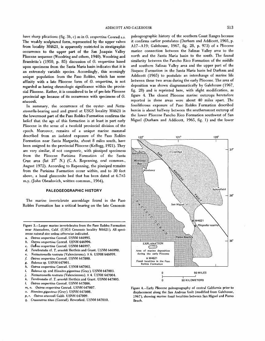
SODA CREEK SPRINGS-METAMORPHIC WATERS IN THE EASTERN ALASKA RANGE
By D. H. RICHTER, R. A. LAMARRE 1 ,
and D. E. DONALDSON, Anchorage, Alaska
Abstract. The Soda Creek springs are a group of small, cold mineral springs on the southern flank of the eastern Alaska Range. The spring waters contain anomalous concentrations of carbon dioxide, sodium, chlorine, sulfate, boron, and ammonia and are actively precipitating deposits of calcite and aragonite. Sparingly present in these deposits are mixed-layer illite-montmorillonite clays and zeolite minerals. Low- temperature metamorphic reactions in subjacent marine sedimentary rocks of Jurassic and Cretaceous age may have produced the fluids and silicate minerals. With only a few exceptions, cool bicarbonate-rich springs in Alaska are concentrated south of the Denali fault system in south-central Alaska, southeastern Alaska, and along the Kaltag-Tintina fault system. These areas are characterized by active or recently active tectonism, major faults and folds, and an abundance of marine sedimentary rocks.
The Soda Creek springs are a group of small, cold sodium- bicarbonate springs on the south flank of the eastern Alaska Range in southern Alaska. The unusual waters of the springs are characteristic of fluids of metamorphic origin (White, 1957b) and hence lend support to the concept of an active metamorphic-tectonic belt rimming the Pacific coast of North America (Barnes, 1970). Ecologically, the springs provide a source of essential minerals and salts to many animals of the area. Critically important is the dependence on the springs of many hundreds of Dall sheep (Ovis dalli), a species unique to Alaska and parts of neighboring Canada.
The springs have been named after their location on Soda Creek, a small tributary of Platinum Creek which drains into the Nabesna River. They occur at an elevation of about 3,600 feet in sec. 26, T. 9 N., R. 13 E., Copper River meridian, in the southeast corner of the Nabesna C-4 quadrangle (scale 1:63,360), and are most easily reached by a series of horse and tractor trails, approximately 11 miles long, that begin at Lost Creek on the Slana-Nabesna Road.
This note summarizes the field and laboratory data made available from several visits to the springs between 1965 and 1970 during the course of the U.S. Geological Survey's
1 Present address: Bath, N.H.
mapping program in the eastern Alaska Range and briefly discusses the geologic significance of the springs. The only known previous references to the springs are a very brief mention of their occurrence and a photograph by Moffit (1933, p. 140; 1941, pi. 6), who conducted a geologic reconnaissance of the area in 1931. Most of our data are derived from a trip during September 9 12, 1970, made especially to map the springs in detail and to sample the spring and nearby surface waters. We thank our colleagues R. M. Chapman and A. L. Clark for their unpublished chemical analyses of water from two Alaskan springs and Professor Robert C. Reynolds, of Dartmouth College, who aided in the X-ray studies of mineral deposits of the Soda Creek springs.
GEOLOGIC SETTING
Two distinct geologic terranes compose the bedrock in the vicinity of the Soda Creek springs. The older terrane, referred to as the Taku-Skolai terrane by Berg, Jones, and Richter (1972), consists of a series of low-grade regionally meta morphosed volcanic and sedimentary rocks ranging in age from Pennsylvanian to Late Triassic. The younger terrane, called the Gravina-Nutzotin belt by the same authors, consists principally of upper Mesozoic marine sedimentary rocks.
The oldest rocks in the Taku-Skolai terrane are a thick and complex series of Pennsylvanian and Permian volcanic and volcaniclastic rocks that are remnants of a late Paleozoic andesite island arc which apparently developed directly on oceanic crust (Richter and Jones, 1970). This old arc assemblage is overlain by nonvolcanogenic Permian marine argillite and minor limestone and Middle and (or) Late Triassic basalt and Late Triassic shallow-water limestone. Rocks of the younger Gravina-Nutzotin belt, unconformably overlying the Taku-Skolai terrane, consist of a thick flyschlike succession of Upper Jurassic and Lower Cretaceous argillite, graywacke, and conglomerate that were deposited in a deep, linear marine basin.
Dikes, sills, and other small irregular hypabyssal intrusions, mafic to intermediate in composition, are common throughout
523
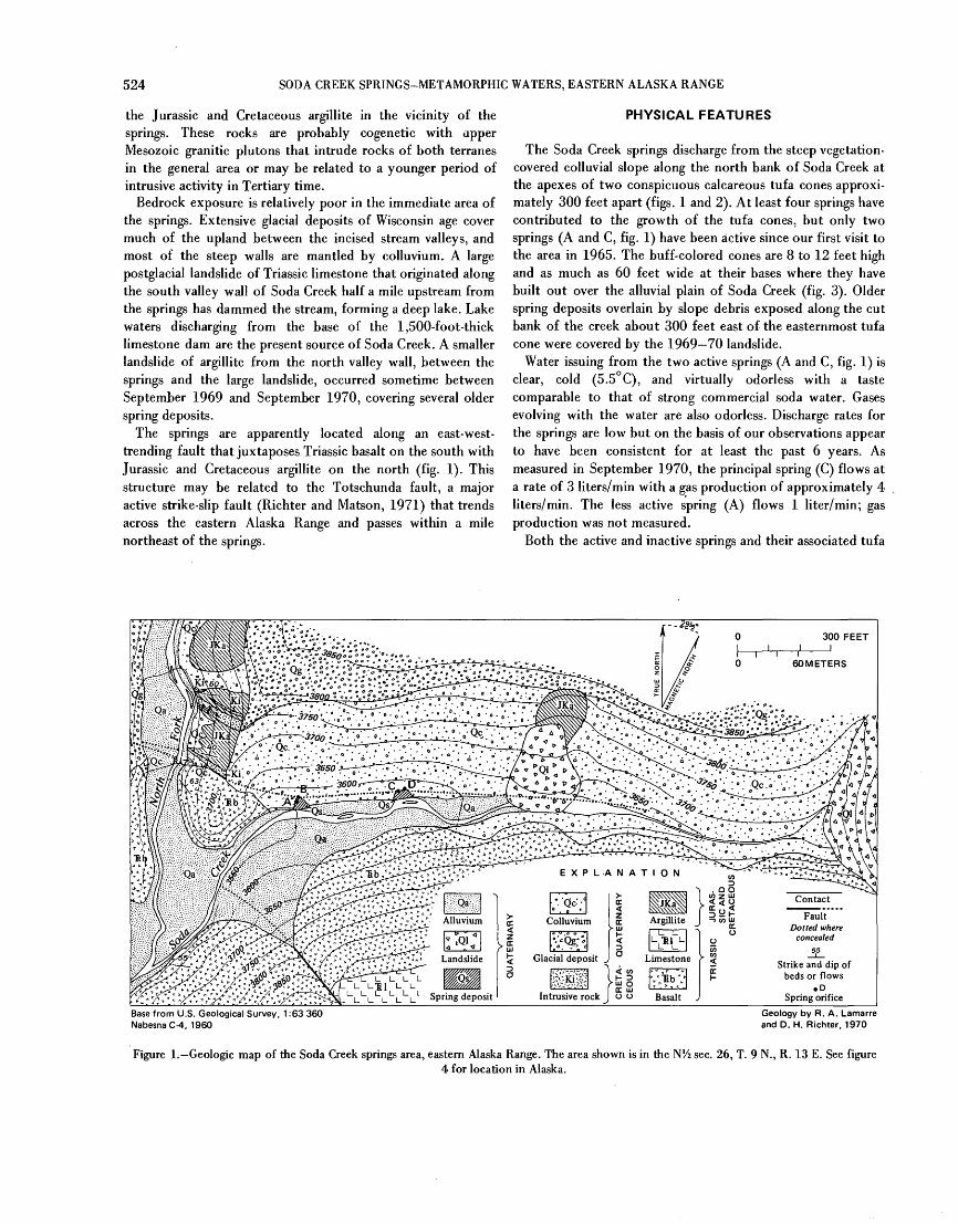
524 SODA CREEK SPRINGS-METAMORPHIC WATERS, EASTERN ALASKA RANGE
the Jurassic and Cretaceous argillite in the vicinity of the springs. These rocks are probably cogenetic with upper Mesozoic granitic plutons that intrude rocks of both terranes in the general area or may be related to a younger period of intrusive activity in Tertiary time.
Bedrock exposure is relatively poor in the immediate area of the springs. Extensive glacial deposits of Wisconsin age cover much of the upland between the incised stream valleys, and most of the steep walls are mantled by colluvium. A large postglacial landslide of Triassic limestone that originated along the south valley wall of Soda Creek half a mile upstream from the springs has dammed the stream, forming a deep lake. Lake waters discharging from the base of the 1,500-foot-thick limestone dam are the present source of Soda Creek. A smaller landslide of argillite from the north valley wall, between the springs and the large landslide, occurred sometime between September 1969 and September 1970, covering several older spring deposits.
The springs are apparently located along an east-west- trending fault that juxtaposes Triassic basalt on the south with Jurassic and Cretaceous argillite on the north (fig. 1). This structure may be related to the Totschunda fault, a major active strike-slip fault (Richter and Matson, 1971) that trends across the eastern Alaska Range and passes within a mile northeast of the springs.
PHYSICAL FEATURES
The Soda Creek springs discharge from the steep vegetation- covered colluvial slope along the north bank of Soda Creek at the apexes of two conspicuous calcareous tufa cones approxi mately 300 feet apart (figs. 1 and 2). At least four springs have contributed to the growth of the tufa cones, but only two springs (A and C, fig. 1) have been active since our first visit to the area in 1965. The buff-colored cones are 8 to 12 feet high and as much as 60 feet wide at their bases where they have built out over the alluvial plain of Soda Creek (fig. 3). Older spring deposits overlain by slope debris exposed along the cut bank of the creek about 300 feet east of the easternmost tufa cone were covered by the 1969 70 landslide.
Water issuing from the two active springs (A and C, fig. 1) is clear, cold (5.5 C), and virtually odorless with a taste comparable to that of strong commercial soda water. Gases evolving with the water are also odorless. Discharge rates for the springs are low but on the basis of our observations appear to have been consistent for at least the past 6 years. As measured in September 1970, the principal spring (C) flows at a rate of 3 liters/min with a gas production of approximately 4 liters/min. The less active spring (A) flows 1 liter/min; gas production was not measured.
Both the active and inactive springs and their associated tufa
300 FEET
FaultDotted where
concealed55
Strike and dip of beds or flows
D Spring orifice
Base from U.S. Geological Survey, 1:63 360 NabesnaC-4, 1960
Geology by R. A. Lamarre and D. H. Richter, 1970
Figure 1. Geologic map of the Soda Creek springs area, eastern Alaska Range. The area shown is in the N'/2 sec. 26, T. 9 N., R. 13 E. See figure4 for location in Alaska.
RICHTER, LAMARRE, AND DONALDSON 525
Figure 2. General view of springs area, looking east up Soda Creek. Springs A and B are at extreme left, and springs C and D are in center partly hidden by leaning spruce tree. In middle background Soda Creek is dammed by 1969 70 landslide (LI) and in background by large limestone landslide (L2).
cones are relatively young features, probably not more than a few thousand years old. A log buried in the upper part of the tufa cone below inactive spring D has been radiocarbon dated in the laboratory of the U.S. Geological Survey (sample W-2567) at 570±250 years B.P. At the other extreme, all the cones undoubtedly have developed since the last Wisconsin glacial advance flushed the valleys of Soda and Platinum Creeks approximately 6,000 to 10,000 years ago.
CHEMISTRY OF THE SPRING WATERS
An analysis of the Soda Creek springs water (spring C) is shown in table 1. For purposes of comparison, an analysis of nearby surface water collected from Soda Creek where it discharges from the limestone dam is also shown. Water samples were filtered through 0.45jU Millipore membranes, and both a raw sample and an acidified sample (to prevent precipitation of calcium carbonate) of the filtered water were saved for analytical purposes.
The waters discharging at the springs are sodium-bicarbonate waters with high concentrations of sodium and carbon dioxide (as indicated by the high HC0 3~ and low pH), a high HCOa'/Cl" ratio, and almost neutral pH. The waters are also rich in calcium, magnesium, potassium, ammonia, boron, sulfate, and chloride. The reported concentration of NH 4+ (11 mg/1) probably represents a minimum value, as the water samples were stored several months prior to the boron and ammonia analyses. No attempt was made to analyze the copious gases evolving with the water. However, field tests showing that the gas neither supports combustion nor is combustible suggest that it is composed largely of C02 . Furthermore, the lack of any appreciable odor is evidence against the presence of any significant amounts of H 2 S.
BFigure 3. Tufa cones at springs C and D. A, Cones below principal
spring C (left) and inactive spring D (right). View north across Soda Creek. B, Closeup of tufa presently being deposited on cone below spring C.
MINERALOGY OF THE SPRING DEPOSITS
The tufa cones are built of many hundreds of thin porous layers of precipitated calcium carbonate (fig. 3) containing lesser amounts of other minerals and locally abundant organic debris. Random samples of travertine collected from both the active and inactive cones range from 67 to 97 weight percent total carbonate with both calcite and aragonite present (table 2). The remainder of the travertine consists of illite-mont- morillonite mixed-layer clay, epsomite, quartz, and minor amounts of gypsum, anhydrite, marcasite, analcite, natrolite, and clinoptilotite(?). Only the epsomite, which is relatively common, and the rarer gypsum may be primary precipitates.

526 SODA CREEK SPRINGS-METAMORPHIC WATERS, EASTERN ALASKA RANGE
Table I. Composition, in milligrams per liter, of Soda Creek springs and meteoric water
[Analysts: D. Donaldson and R. Barnes (B, NH 4+), U.S. Geological Survey]
Source of water ..... Soda Creek springs Nabesna C-4 quadrangle
(lat62°32'N., long 142°56' W.)
PH ...............Temperature (°C). . . .
Si0 2 ..............Fe. ...............Mn ...............Ca ...............Mg ...............Na ...............K...... ..........NH 4 ..............B ................HC0 3 .............SO, ..............a................F ................NO...............
6.85.5
121.8
.2381192
2,220160
11104
7,240580257
.7
.7
Soda Creek (discharge from base of landslide)
7.87
6.50
.024811
3.5
.1171
291.5
.1
.4
Table 2. Mineral composition of travertine from the Soda Creek springs tufa cones
SpringCarbonate content,in percent (calcite
and aragonite)'Other minerals2
A (discharge rate, 1liter/min).
B (inactive)......
C, at orifice (dis charge rate, 3 liters/min).
C ............
D (inactive).
81
97
80
92
67
Illite-montmorillonite, epsomite, quartz.
Illite-montmorillonite, quartz, clinoptilo- lite(?), marcasite.
Illite-montmorillonite, epsomite, quartz.
Illite-montmorillonite, epsomite, anhydrite.
Illite-montmorillonite, epsomite, gypsum, anhydrite, analcite, natrolite.
1 Amount determined by loss in weight after acetic acid leach.2 Determined by X-ray diffraction of insoluble residue remaining after
acetic acid leach.
Most of the other minerals are apparently carried up as participate matter by the spring waters, although some (especially the quartz, and possibly the gypsum and anhydrite) may be of clastic windblown origin.
In the older spring deposits, covered by the 1969 70 landslide, the travertine contained small, irregular masses of marcasite associated with epsomite and antlerite, suggesting that at one time the springs were highly charged with H2 S. Also indicative of an earlier stage of higher sulfur activity are the abundant gypsum-anhydrite veins that lace the Jurassic and Cretaceous argillite peripheral to the springs.
ORIGIN
The unusual chemistry of the Soda Creek springs water and extremely large concentrations of many of its anomalous components argue against a meteoric origin for most of the water. Thermal waters of somewhat similar composition are known from a few active volcanic areas the volcanic sodium- bicarbonate type water of White (1957a, p. 1649 1651) but there is no geologic evidence in the eastern Alaska Range that the Soda Creek springs are related to present or recently active volcanism. White (1957a) recognized that not all sodium- bicarbonate waters are associated with areas of active vol canism and. in a companion paper (White, 1957b, p. 1678 1679) suggested that many of these nonvolcanic high- bicarbonate waters may be fluids derived from the low-grade metamorphism of marine sedimentary rocks. In addition to the high bicarbonate content, White's criteria for metamorphic water included normal to low temperature, anomalous concen trations of boron and ammonia, and relatively low chloride compared with sea water.
On the basis of these criteria, the waters from the Soda Creek springs are considered to be mostly of metamorphic origin. The source from which these fluids and their unusual components have been derived is very likely the thick sequence of Jurassic and Cretaceous marine sedimentary rocks that underlie the springs area. An alternate source is the older and more deeply buried marine argillites and interbedded impure limestones of Permian age that occur at depths estimated to range from 5,000 to 8,000 feet beneath the springs. However, these Permian rocks have been regionally metamorphosed as high as the pumpellyite facies and conse quently may already have lost much of their water and constituents such as boron, ammonia, and chlorine.
The mixed-layer clays and zeolite minerals found in the travertine precipitated by the springs lend additional support for a metamorphic origin of waters. Nowhere in surface exposures of either the Jurassic and Cretaceous argillites or the older Permian marine sedimentary rocks have these minerals been observed. X-ray studies of the fine-grained matrices of the Jurassic and Cretaceous argillites show the presence of quartz, both K-feldspar and Na-Ca-feldspars, calcite, chlorite,
and possibly pyrophyllite. In the Permian rocks chlorite, pumpellyite, epidote, and albite have been recognized. Hence it appears that the clay and zeolites are authigenic species resulting from metamorphic reactions at depth beneath the springs. Although the temperatures and pressures in the source rocks must be relatively low, Muffler and White (1969) have shown that significant reactions involving silicate minerals occur at temperatures below 100 C.
SIGNIFICANCE OF THE SODA CREEK SPRINGS AND OTHER METAMORPHIC WATERS IN ALASKA
Recently, Barnes (1970) has reiterated and strongly sup ported White's suggestion of a metamorphic origin for many
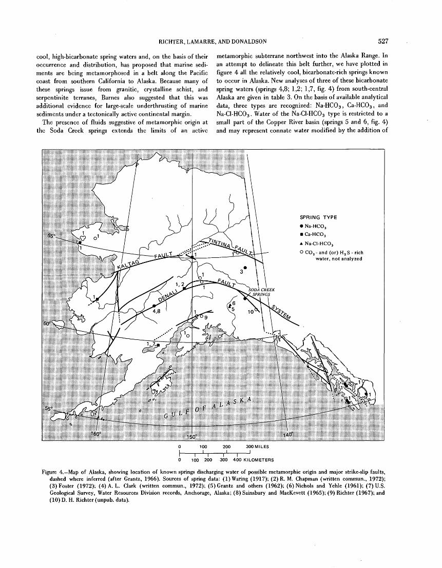
RICHTER, LAMARRE, AND DONALDSON 527
cool, high-bicarbonate spring waters and, on the basis of their occurrence and distribution, has proposed that marine sedi ments are being metamorphosed in a belt along the Pacific coast from southern California to Alaska. Because many of these springs issue from granitic, crystalline schist, and serpentinite terranes, Barnes also suggested that this was additional evidence for large-scale underthrusting of marine sediments under a tectonically active continental margin.
The presence of fluids suggestive of metamorphic origin at the Soda Creek springs extends the limits of an active
metamorphic subterrane northwest into the Alaska Range. In an attempt to delineate this belt further, we have plotted in figure 4 all the relatively cool, bicarbonate-rich springs known to occur in Alaska. New analyses of three of these bicarbonate spring waters (springs 4,8; 1,2; 1,7, fig. 4) from south-central Alaska are given in table 3. On the basis of available analytical data, three types are recognized: Na-HCOs, Ca-HC0 3 , and Na-Cl-HC0 3 . Water of the Na-Cl-HC0 3 type is restricted to a small part of the Copper River basin (springs 5 and 6, fig. 4) and may represent connate water modified by the addition of
SPRING TYPE
Na-HCO 3
Ca-HCO 3
A Na-Cl-HCO 3
O CO 2 -and (or) HjS-rich water, not analyzed
100 200 300 MILES_J______I______I
I I I I I0 100 200 300 400 KILOMETERS
Figure 4. Map of Alaska, showing location of known springs discharging water of possible metamorphic origin and major strike-slip faults, dashed where inferred (after Grantz, 1966). Sources of spring data: (1) Waring (1917); (2) R. M. Chapman (written commun., 1972); (3) Foster (1972); (4) A. L. Clark (written commun., 1972); (5) Grantz and others (1962); (6) Nichols and Yehle (1961); (7) U.S. Geological Survey, Water Resources Division records, Anchorage, Alaska; (8) Sainsbury and MacKevett (1965); (9) Richter (1967); and (10) D. H. Richter (unpub. data).

528 SODA CREEK SPRINGS-METAMORPHIC WATERS, EASTERN ALASKA RANGE
Table 3. Chemical composition, in milligrams per liter, of other bicarbonate springs in Alaska
[Analysts: R. Barnes, 1970 (White Mountain springs); B. Walling, 1957 (Kantishna springs); C. L. Barwis, 1968 (Kakhonak springs), all U.S. Geological Survey]
1
Source of water
1
pHTempera
ture (°C)
Si0 2 .....Fe ......Ca. ......Mg ......Na ......K .......B .......HC0 3 .... S0 4 .....Cl .......F .......N0 3 .....
SVhite Mountain springs (4,8)' , McGrath A-4
quadrangle (lat62°10'N., ong!54°53'W.)
Cool
5043
1843.31.0
632 160
5.3
Kantishna springs (1,2), Mount McKinley C-2
quadrangle (lat63°31'N.,
1 longl50°59'W.)
6.2
6
366.8
405347210
8
1,960 90
8500
Kakhonak springs (1,7), Iliamna B-5 quadrangle (lat59°28'N.,
long 154° 31' W.)
4
57
369106275
13
2,310 4476
.2
.3
1 Numbers in parentheses refer to localities in figure 4.
volcanic or metamorphic water or both (Grantz and others, 1962, p. 2000-2001).
Significantly, most of the cool bicarbonate springs of Alaska occur in southeastern Alaska, generally west of the Coast Range plutonic belt, and in south-central Alaska either along the Denali fault system or between the fault system and the continental margin. This terrane is composed chiefly of late Paleozoic and younger rocks, including widespread, thick marine sedimentary deposits. South of the Denali fault system in south-central Alaska between long 141° and 152 W., this terrane is thought to be virtually decoupled from the older terrane north of the fault (North American plate) and to be actively undergoing strong compressional deformation owing to the northward movement and impingement of the Pacific plate (Richter and Matson, 1971). In southeastern Alaska,
similar deformation apparently prevailed as recently as late Tertiary time, underthrusting Mesozoic marine sedimentary rocks beneath the Coast Range plutons (Berg and others, 1972).
A few bicarbonate-rich springs occur along the Kaltag, Tintina, and related faults extending across central Alaska north of the Denali fault system. These major faults transect thick sequences of Paleozoic and Mesozoic marine sedimentary rocks and may in part represent tectonic boundaries between old crustal plates.
Only a cluster of springs on the Seward Peninsula in western Alaska and one spring in east-central Alaska (spring 3, fig. 4) do not appear to be related to young major structures and do
not occur in areas underlain by marine sedimentary rocks. In both areas the terrane consists chiefly of Precambrian and old Paleozoic metamorphic rocks now part of a stable continental platform. Mesozoic and Cenozoic intrusive rocks cut the metamorphic rocks near the bicarbonate spring in east-central Alaska (Foster, 1972) and may explain the presence of the unusual water, but on the Seward Peninsula, no ready explanation for the springs is available.
In summary, we suggest that the Soda Creek springs and most of the other anomalous cool bicarbonate-rich springs in Alaska are discharging fluids characteristic of metamorphic origin. Except for the few springs on the Seward Peninsula and the one in east-central Alaska, all occur in terranes of present or recently active tectonism that include thick sections of marine sedimentary rocks, and many are located along major structures within these terranes.
REFERENCES CITED
Barnes, Ivan, 1970, Metamorphic waters from the Pacific tectonic belt of the west coast of the United States: Science, v. 168, p. 973-975.
Berg, H. C., Jones, D. L., and Richter, D. H., 1972, Gravina-Nutzotin belt Tectonic significance of an upper Mesozoic sedimentary and volcanic sequence in southern and southeastern Alaska, in Geologi cal Survey Research 1972: U.S. Geol. Survey Prof. Paper 800-D, p. D1-D24.
Foster, H. L., 1972, Preliminary geologic map of the Eagle quadrangle, Alaska: U.S. Geol. Survey Misc. Field Studies Map MF-358.
Grantz, Arthur, 1966, Strike-slip faults in Alaska: U.S. Geol. Survey open-file report, 82 p.
Grantz, Arthur, White, D. E., Whitehead, H. C., and Tagg, A. R., 1962, Saline springs, Copper River lowland, Alaska: Am. Assoc. Petroleum Geologists Bull., v. 46, p. 1990-2002.
Moffit, F. H., 1933, The Suslota Pass district, upper Copper River region, Alaska: U.S. Geol. Survey Bull. 844-C, p. 137-162.
1941, Geology of the upper Tetling River district, Alaska: U.S.Geol. Survey Bull. 917-B, p. 115-157.
Muffler, L. J. P., and White, D. E., 1969, Active metamorphism ofupper Cenozoic sediments in the Salton Sea geothermal field andthe Salton trough, southeastern California: Geol. Soc. AmericaBull., v. 80, p. 157-182.
Nichols, D. R., and Yehle, L. A., 1961, Mud volcanoes in the CopperRiver basin, Alaska, in Rausch, G. 0., ed., Geology of the Arctic:Internat. Symposium on Arctic Geology, 1st, Calgary 1960, Proc., v.2, p. 1063-1087.
Richter, D. H., 1967, Geological and geochemical investigations in theMetal Creek area, Chugach Mountains, Alaska: Alaska Div. Minesand Minerals Geol. Rept. 25, 17 p.
Richter, D. H., and Jones, D. L., 1970, Structure and stratigraphy ofthe eastern Alaska Range [abs.]: Am. Assoc. Petroleum GeologistsBull., v. 54, p. 2502.
Richter, D. H., and Matson, N. A., Jr., 1971, Quaternary faulting in theeastern Alaska Range: Geol. Soc. America Bull., v. 82, p.1529-1540.
Sainsbury, C. L., and MacKevett, E. M., Jr., 1965, Quicksilver depositsof southwestern Alaska: U.S. Geol. Survey Bull. 1187, 89 p.
Waring, G. A., 1917, Mineral springs of Alaska: U.S. Geol. SurveyWater-Supply Paper 418,114 p.
White, D. E., 1957a, Thermal waters of volcanic origin: Geol. Soc.America Bull., v. 68, p. 1637-1658.
1957b, Magmatic, connate, and metamorphic waters: Geol. Soc. America Bull., v. 68, p. 1659-1682.

Jour. Research U.S. Geol. Survey Vol. l,No.6,Sept.-Oct. 1973, p. 529 634
THE DUN MOUNTAIN ULTRAMAFIC BELT- PERMIAN OCEANIC CRUST AND UPPER MANTLE
IN NEW ZEALAND
By M. C. BLAKE, JR., and C. A. LANDIS 1 ,
Washington, D.C., Dunedin, New Zealand
Abstract. Geologic evidence suggests that the Dun Mountain ultra- mafic belt in New Zealand is the basal part of a Lower Permian ophiolite suite. By analogy with other ophiolite suites, and as a result of marine geophysical studies of the present ocean basins, the ophiolite is believed to represent oceanic crust and upper mantle upon which the Upper Permian Maitai Group was deposited. After this, much of the ultramafic belt was extensively deformed to tectonic melange.
This paper proposes that the Dun Mountain ultramafic belt constitutes the tectonically disrupted basal part of a Lower Permian ophiolite suite which originally stratigraphically underlaid the eastern margin of the Hokonui facies of the New Zealand geosyncline.
The Dun Mountain ultramafic belt (Landis and Coombs, 1967) consists of two widely separated belts of ultramafic rock within the New Zealand geosyncline (fig. 1). One belt is on the southeast side of the Alpine fault (Red Mountain part); the other (Dun Mountain part) is on the northwest side of the fault and includes the type locality for dunite. They are considered to have been one continuous belt before a 480-km strike-slip displacement along the Alpine fault.
Acknowledgments. The writers' research has been sup ported by grants from the U.S. National Science Foundation (g/18700) and New Zealand University Grants Committee (C. A. Landis) and the Fulbright Commission and Auckland University Fellowship (M. C. Blake, Jr.). The manuscript has benefitted from discussion and criticism by D. S. Coombs, E. H. Bailey, and T. P. Thayer.
HISTORICAL BACKGROUND
The origin of the Dun Mountain rocks has long been debated, and a brief review of selected interpretations is presented here. As early as 1864, the existence of an elongate belt of ultramafic rock passing through the Dun Mountain region was recognized (Hochstetter, 1864). Hochstetter was
' Department of Geology, University of Otago.
impressed by the overall conformity between the ultramafic belt and adjoining country rock (upper Paleozoic sedimentary rock and volcanic rock) and suggested that the ultramafic rock originated as a sill-like intrusion. Other early workers were equally impressed with the regular, seemingly stratigraphic, contact between the ultramafic-volcanic suite and the overly ing limestones of the Maitai Group (Upper Permian), and McKay (1879) interpreted this relationship as indicating that the ultramafites and associated basaltic rocks were already on the sea floor (possibly originating as lava flows) when the Maitai limestone was deposited.
Later a post-Maitai intrusive origin for the Dun Mountain ultramafic belt came into vogue. An intrusive origin was first proposed by Park (1887, 1921) and was later developed and popularized by W. N. Benson (1926). Benson envisaged the ultramafites as intrusions, probably in a semisolid state, along major Mesozoic thrust faults. Many subsequent workers (Turner, 1930, Macpherson, 1946; Kingma, 1959) continued to favor Mesozoic intrusion along a great thrust zone.
A return to the McKay hypothesis favoring penecontem- poraneity of the ultramafites with Lower Permian spilites, dolerites, and associated sediments was proposed by Grindley (1958). Grindley mapped a large segment of the Red Mountain part of the Dun Mountain belt and suggested that the ultramafites (mainly serpentinites) originated as submarine lava flows. Early Permian origin of the ultramafites was also favored by Waterhouse (1964, p. 87): "Near the close of the Lower Permian serpentine was emplaced laterally, accom panied by mild orogeny***."
Recent detailed studies of selected areas within the Dun Mountain part of the ultramafic belt by G. A. Challis, W. R. Lauder, and R. I. Walcott have led to the hypothesis of high-temperature emplacement of ultramafic magma into Lower Permian volcanic rocks. The presence of a high- temperature ultramafic intrusion in the Dun Mountain area (Lauder, 1965a,b; Challis and Lauder, 1966) is inferred from (1) structural discontinuities between peridotites (and asso ciated serpentinites) and Maitai Group sedimentary rocks of
529

530 DUN MOUNTAIN ULTRAMAFIC BELT-PERMIAN OCEANIC CRUST, MANTLE
) EXPLANATION [
J V
200 MILES I______I
0 100 200 KILOMETERS i i I I I
Figure 1. Map showing location of Dun Mountain ultramafic belt, South Island, New Zealand. Localities corresponding to sections in figure 3: 1, Port Hardy, D'Urville Island; 2, Taipare, Tasman Bay; 3, Dun Mountain-Wooded Peak area; 4, Red Hills; 5, Matakitaki; 6, Red Mountain; 7, Cascade Creek; 8, Annear Creek-Upukerora Valley area. Eastern province comprises New Zealand geosyncline and contempo raneous intrusive rocks along western side of geosyncline. Hokonui belt is within eastern province west of Dun Mountain belt and southwest of Livingstone-Macpherson fault system. Western province comprises crystalline and moderate- to high-temperature-pressure metamorphosed Paleozoic rocks (Landis and Coombs, 1967). Median tectonic line is a zone of dislocation (Landis and Coombs, 1967) marking western margin of New Zealand geosyncline. Livingstone- Macpherson fault system is the boundary between two contrasting geosynclinal assemblages (Landis and Bishop, 1972). The northern extent of this fault system coincides with eastern margin of Dun Mountain ultramafic belt.
Late Permian age, (2) apparently steeply inclined concentric lithologic layering of dunite and peridotite within the Dun Mountain massif, and (3) contact metamorphism of adjoining Maitai Group country rock. Lauder (1965a, b) concluded that Dun Mountain is a volcanic pipe or magma chamber formed at the root of a Cretaceous volcano. At Red Hills, 45 km south of Dun Mountain, another large peridotite mass was described by Challis (1965a, b) and Walcott (1969). Challis regarded it as a high-temperature lopolithic intrusion. The peridotite contains
near-horizontal cumulate layering that contrasts with near- vertical layering in adjoining Lower Permian spilite, a situation which seems to require deformation before emplacement of the ultramafic liquid. Evidence cited in favor of high-tempera ture intrusion is chiefly the unfaulted contact between cumulate ultramafite and pyroxene hornfels-facies country rock. Challis regarded the spilites and ultramafites as geneti cally related rocks and proposed intrusion of ultramafic liquid into deformed but comagmatic spilite. The Red Hills body was regarded as the crystallized contents of a large magma chamber at a high level within a Permian volcanic arc. Walcott (1969) also interpreted Red Hills as a high-temperature magmatic intrusion of Permian age; however, some of his observations conflict with those of Challis (see below). Both the Dun Mountain and Red Hills peridotite masses appear to be rootless; this has been interpreted (Challis and Lauder, 1966) as being due to later low-angle thrust faults.
DISCUSSION OF HYPOTHESES
We cannot fully agree with any of the origins proposed for the Dun Mountain belt, or for selected parts thereof. Some specific points of contention and our contrary interpretations are:
1. Emplacement of ultramafites along a major Mesozoic thrust fault (Benson, 1926). The intimate association and regionally concordant relation between ultramafites and the suite of Permian volcanic rocks, limestones, and volcanogenic sedimentary rocks is too widespread for us to accept a hypothesis requiring a separate and distinctive origin for each suite (see also Grindley, 1958). On the contrary, we believe that the volcanic rocks and the ultramafites are genetically related. We do acknowledge, however, a relation between Mesozoic thrust faulting and the present distribution of ultramafites brought about by localization of thrusting along a preexisting zone of weakness corresponding to both the incompetent serpentinite and an ancient plate margin (Landis and Bishop, 1972).
2. Suggested origin of ultramafic rock as submarine flow (Grindley, 1958). We agree with Grindley that gabbroic and ultramafic rocks were on, or at least near to, the Permian sea
floor when spatially associated volcanic materials were em- placed. However, we can find no evidence for flows of ultramafic lava. Neither our field observations nor those of marine geologists (for example, JOIDES deep-sea drilling) provide any reason to favor extrusion of voluminous ultra- mafic liquid onto the sea floor.
3. Is Dun Mountain a volcanic neck? (Lauder, 1965a, b). Walcott (1969) has already discussed some of the short comings of this hypothesis: for example, there is no com pelling evidence for intrusive contacts with Maitai rocks, whose thermal metamorphism, as described by Lauder, can be explained by low-temperature contact metasomatic effects (Coleman, 1966). In addition, no convincing evidence for a

BLAKE AND LANDIS 531
cylindrical form of the Dun Mountain body has been presented, and the orientation of mineral layering reported by Walcott and confirmed by us conflicts with data presented by Lauder. The absence of any other evidence for Cretaceous volcanism in the Dun Mountain region (for example, mafic- ultramafic pyroclastic deposits) is noteworthy (Chain's, 1965a, b).
4. Shallow roots of a Permian volcanic arc (Challis, 1965a). Challis regarded the Red Hills peridotite body as being emplaced as an ultramafic magma into a comagmatic Permian volcanic arc. Evidence to support this hypothesis includes a high-temperature unfaulted contact between the ultramafic rock and the comagmatic volcanic rocks. A fundamental problem with this hypothesis is the enormous size required for a relatively shallow magma chamber (present size of ultramafic outcrop at Red Hills is 9 by 10 km) which was emplaced beneath, but apparently never broke through, a thin (1-km) carapace of penecontemporaneous volcanic rock. In addition, significant discrepancies exist between Challis' map of the western margin of the Red Hills body and mapping by Walcott (1969), and reconnaissance studies by one of us (Landis, 1969). In particular, whereas no faults were mapped in this area by Challis, many faults in the western part of the ultramafic body were mapped by Walcott. One of these faults appears to be a major fault parallel to the ultramafite volcanic rock contact. In addition, the presence of serpentinite adjacent to the western, supposedly high-temperature intrusive contact, and a parallel dikelike mass of serpentinite 100 m farther west, along with field data discussed elsewhere in this paper, suggest that the Red Hills mass may be part of a melange belt. Furthermore, chemically analyzed pyroxenes from Red Hills (Challis, 1965a) have been plotted by O'Hara (1967) on his pressure-temperature grid showing estimated conditions of equilibration of some natural ultramafic assemblages. Crystalli zation of Red Hills pyroxenes is estimated at 1,100°C 4 kb. This corresponds to depths of 10 15 km (depending on density of overburden), a conclusion consistent with Walcott's observations of tectonite fabrics and folding in the Red Hills peridotites. Identical fabrics have been described from many other alpine ultramafic rocks (Coleman, 1971, p. 1214 1215) and attributed to high-temperature mantle deformation.
PLATE TECTONIC INTERPRETATION
Recent mapping, coupled with interpretation guided by concepts of global tectonics, has led us to propose that the Dun Mountain belt constitutes a deformed, and in part remobilized, oceanic basement of Permian age (Landis, 1969; Hatherton, 1969) on which the Permian Maitai sedimentary rocks were deposited. On the basis of analogy with the ophiolite basement which underlies the Great Valley sequence of California (Bailey and others, 1970), a similar hypothesis has been proposed by Dickinson (1971).
Our recent mapping in the Nelson-Mar Iborough Sounds regions supports the oceanic-crust hypothesis. Our data, along
with field and petrologic observations by other workers throughout the length of the Hokonui terrane (as defined by Landis and Bishop, 1972), permit a reasonably detailed actualistic interpretation of the origin of the Dun Mountain ultramafic belt and also of the associated Permian volcanic and sedimentary rocks (Lee River and Humboldt Groups of Waterhouse, 1964).
Marine geophysical studies indicate a remarkably constant ocean-basin structure (Raitt, 1963) a sequence progressing downward through a representative part of the sea floor is believed to comprise:
Crustal layer 1 sediments (mainly pe- 0 1.0km lagic mud, chert, bio- genie carbonate).
Crustal layer 2 pillow basalt and dia- 1.6 2.0kmbase.
Crustal layer 3 gabbro, amphibolite, 4.8 km metabasalt (± dio- rite, trondhjemite, serpentinite).
M DiscontinuityUpper mantle harzburgite and dunite,
probably underlain by Iherzolite and garnet peridotite.
The ocean-basin sequence, although generally somewhat thicker, is similar to the ophiolite suite, a partly layered rock assemblage characteristic of some erogenic belts. Typically, the ophiolite suite consists (from base to top) of dunite and peridotite (variably serpentinized) overlain by gabbro and amphibolite, pillow basalts, and capped by pelagic sediments (Moores and Vine, 1971). Several workers (Bailey and others, 1970; Davies, 1971; Coleman, 1971; Dewey and Bird, 1971; Bezzi and Piccardo, 1971) have emphasized that rock se quences and thicknesses of documented ophiolite suites are comparable to the oceanic crust upper mantle. Stratigraphic sections from Permian geosynclinal sediments downward into the Dun Mountain rocks (figs. 2 and 3) also resemble an ocean-floor sequence (see also Coleman, 1966, figs. 5,25,40, and 41). The main contrasts between the Dun Mountain ophiolites and the oceanic sequences are (1) the generally sheared and incompletely developed sequences which charac terize the Dun Mountain belt, and (2) the consistently thinner nature of layer 2 and layer 3 rocks of the Dun Mountain belt in comparison with oceanic crust. We believe that these discrepancies are due in part to intensive post-Permian tectonism and in part to original differences in thickness.
In most areas, we find the Dun Mountain ophiolite belt to be a tectonic melange. Tectonic blocks of sedimentary, volcanic, gabbroic, and ultramafic rock occur as inclusions within a matrix of sheared serpentinite and argillite. Field relationships, petrography, and metasomatic alteration of these blocks were described by Coleman (1966), and our

532 DUN MOUNTAIN ULTRAMAFIC BELT-PERMIAN OCEANIC CRUST, MANTLE
Cl'O O p O O
k' \ A T I \
- 1 KILOMETER
Figure 2. Interpretive reconstruction of a representative stratigraphic section of undeformed Permian sea floor (Dun Mountain ophiolites), eastern margin of Hokonui belt. A, Peridotite, dunite, and less commonly Iherzolite; variably serpen-
tinized; rodingitized gabbroic to basaltic dikes. B, Serpentinite and argillite, generally sheared. C, Gabbro, dolerite, amphibolite, minor trondhjemite; extensively
albitized and rodingitized; locally thermally metamorphosed. D, Basaltic lava, massive and layered, largely spilitized. E, Agglomerate plus volcanic-hypabyssal breccias. F, Pillow lava, extensively spilitized. G, Conglomerate and breccia, well to poorly bedded; predominantly
volcanogenic with minor amounts of sedimentary, hypabyssal,and plutonic clasts; some interbedded black argillite andsiliceous sediments.
H, Limestone, composed mainly of bivalvian detritus; calcturbidites;interbedded volcanogenic and minor siliceous sediments.
I, Siltstone and sandstone, fossiliferous, quartz-bearing. J, Sandstone, green and volcanogenic, unfossiliferous. K, Mudstone and fine-grained sandstone, laminated and graded,
unfossiliferous.
studies confirm his account. Outcrop size of the blocks varies from less than 1 m to 2 by 2 km (for example, Dun Mountain massif). At Red Hills, gravity studies (Malahoff, 1965),
detailed regional mapping (Walcott, 1969), and our own reconnaissance observations suggest that this ultramafic body (outcrop area, 10 by 9 km) also may be an enormous tectonic block.
Despite tectonic mixing and frequent juxtaposition of strange bedfellows (for example, peridotite and argillite), an overall ghost stratigraphy appears to persist within parts of the melange; sedimentary and volcanic blocks tend to be more abundant near the upper (western) ophiolite contact, whereas gabbroic and ultramafic blocks are more common deeper (farther east) in the deformed ophiolite. Reduction of original thicknesses of basaltic and gabbroic layers may have occurred by attenuation during rotation of the steep-to-overturned eastern limb of the Nelson Key Summit regional syncline
TTTTT
KILOMETERS
-0
X /"7 \
Figure 3. Selected stratigraphic sections, somewhat diagrammatic, through Dun Mountain ultramafite and associated rocks. Data from Grindley (1958); Waterhouse (1964); Lauder (1965a, b); Walcott (1969); Coleman (1966); Landis (1969); Bell, Clarke, and Marshall (1911); Lensen (1963); Beck (1964); and unpublished work by the authors. Location of sections 1 8 shown in figure 1; section 9 is a representative sequence of oceanic crust and upper mantle. Explana tion of symbols given in figure 2; heavy lines are faults. Melange shown as rounded blocks surrounded by serpentinite; in reality, matrix includes sheared sediment as well.
formed in the Permian sedimentary rocks west of the ultramafic belt. It is also possible that the basaltic and gabbroic rocks of layers 2 and 3 were originally anomalously thin. Rapid spreading rates have been suggested as a possible
cause of thin layer 2 (Moores and Vine, 1971; Dewey and Bird, 1971; Menard, 1967), and a similar origin for thin layer 3 also seems feasible.
Origin of Dun Mountain ophiolites beneath a marginal or interarc basin (Karig, 1971, 1972) should also be given consideration, especially as certain aspects of the Dun Moun tain belt resemble characteristics expected for marginal-basin ophiolites (Dewey and Bird, 1971).
EVOLUTION OF DUN MOUNTAIN ULTRAMAFIC BELT
We propose that the Dun Mountain ultramafic belt origi nated as follows:

BLAKE AND LANDIS 533
1. Permian sea-floor spreading, accompanied by:a. extrusion of submarine basalt along a ridge or
marginal-basin axis;b. crystallization of comagmatic gabbroic rocks deeper
beneath ridge and possibly of comagmatic cumula tive peridotite and dunite beneath gabbro;
c. formation of other peridotites and dunites as residue rocks by partial melting and upward expulsion of basaltic component from Iherzolitic mantle. The Dun Mountain ultramafite comprises these ultra- mafic rocks, plus b (above), plus serpentinized derivatives;
d. regional thermal metamorphism of basaltic and gabbroic rocks to amphibolite and greenschist facies within axial part of ridge or marginal basin;
e. contemporaneous subduction of cooled oceanic crust plus underlying Dun Mountain oceanic man tle beneath an Early Permian volcanic arc (Brook Street terrane).
f. deposition of Permian deep-sea sediments. Volcanic- plutonic breccias derived from layer 2 and layer 3 rocks exposed along fault scarps within ridge. Pelagic muds and calcareous and siliceous sedi ments (including some cherts) deposited upon layer 2 and layer 3 basement on quiet sea floor between ridge and subduction zone or within marginal basin.
2. Late Permian cessation of sea-floor spreading and subduc tion. Sedimentation of flyschoid sediment, predomi nantly of andesitic-basaltic provenance, possibly filling inactive trench (Maitai Group).
3. Folding,2 thrusting, metamorphism, serpentinization, and internal disruption of ophiolite belt: creation of Dun Mountain melange.
4. Division of Dun Mountain belt into Dun Mountain part and Red Mountain part by 480-km strike-slip offset along Alpine fault in Late Cretaceous-Holocene time.
Time of formation of the melange is unclear. Possible melange formation was initiated during Permian-Early Triassic subduction and orogenesis (compare Landis and Bishop, 1972); however, evidence for further deformation or wholesale subduction affecting the Dun Mountain belt does not appear until Late Jurassic Early Cretaceous time, when renewed activity Rangitata orogeny resulted in extensive deforma tion, low-ratio pressure-temperature metamorphism, and melange formation. Deformation of the ophiolite belt has continued locally and spasmodically into the Cenozoic (Flem- ing, 1947).
3 Ophiolite sequences with inferred eastward-facing direction occur in certain areas (Waterhouse, 1964, p. 16, 21 23) and may indicate anticlinal folding of the Dun Mountain belt.
REFERENCES CITED
Bailey, E. H., Blake, M. C., Jr., and Jones, D. L., 1970, On-landMesozoic oceanic crust in California Coast Ranges, in GeologicalSurvey Research 1970: U.S. Geol. Survey Prof. Paper 700-C, p.C70-C81.
Beck, A. C., 1964, Geological map of New Zealand, Sheet 14,Marlborough Sounds: Wellington, New Zealand Geol. Survey, scale1:250,000.
Bell, J. M., darke, E. de C., and Marshall, P., 1911, The geology of theDun Mountain subdivision, Nelson: New Zealand Geol. Survey, newser., Bull. 12, 71 p.
Benson, W. N., 1926, The tectonic conditions accompanying theintrusion of basic and ultrabasic igneous rocks: Natl. Acad. Sci.Mem., v. 19, no. 1, 90 p.
Bezzi, Alfredo, and Piccardo, G. B., 1971, Structural features of theLigurian ophiolites; petrologic evidence for the "oceanic" floor ofthe northern Apennines geosyncline; a contribution to the problemof the alpine-type gabbro-peridotite associations: Soc. Geol. ItalianaMem., v. 10, no. 1, p. 53-63.
Challis, G. A., I965a, The origin of New Zealand ultramafic intrusions:Jour. Petrology, v. 6, no. 2, p. 332-364.
1965b, High-temperature contact metamorphism at the Red Hillsultramafic intrusion, Wairau Valley, New Zealand: Jour. Petrology,v. 6, no. 3, p. 395-419.
Challis, G. A., and Lauder, W. R., 1966, The genetic position of"alpine" type ultramafic rocks: Bull. Volcanol., v. 29, p. 283-304.
Coleman, R. G., 1966, New Zealand serpentinites and associatedmetasomatic rocks: New Zealand Geol. Survey Bull. 76,102 p.
1971, Plate tectonic emplacement of upper mantle peridotitesalong continental edges: Jour. Geophys. Research, v. 76, no. 5, p.1212-1222.
Davies, H. L., 1971, Peridotite-gabbro-basalt complex in eastern Papua:an overthrust plate of oceanic mantle and crust: Australia Bur.Mineral Resources, Geology, and Geophysics Bull. 128, 48 p.
Dewey, J. F., and Bird, J. M., 1971, Origin and emplacement of theophiolite suite; Appalachian ophiolites in Newfoundland: Jour.Geophys. Research, v. 76, no. 14, p. 3179-3206.
Dickinson, W. R., 1971, Clastic sedimentary sequences deposited inshelf, slope, and trough settings between magmatic arcs andassociated trenches: Pacific Geology, v. 3, p. 15 30.
Fleming, C. A., 1947, Serpentinite at Wairere, Totoro survey district,King country: New Zealand Jour. Sci. and Technology, v. 29, no. 3,p. 100-115.
Grindley, G. W., 1958, The geology of the Eglinton Valley, Southland;parts of Eglinton (S131) and Mavora (S141) sheet districts: NewZealand Geol. Survey Bull. 58, 68 p.
Hatherton, Trevor, 1969, Geophysical anomalies over the eu- andmiogeosynclinal systems of California and New Zealand: Geol. Soc.America Bull., v. 80, no. 2, p. 213-230.
Hochstetter, F. C. von, 1864, Geologic von Neu-Seeland. Beitrage zurGeologic der Provinzen Auckland und Nelson, in Reise derOsterreichischen Fregatte Novara um die Erde, in. . .1857 59.Geologischen Theil, v. 1, sec. 1: Vienna, 274 p. (English edition,translation by C. A. Fleming: Wellington, Govt. Printer).
Karig, D. E., 1971, Origin and development of marginal basins in thewestern Pacific: Jour. Geophys. Research, v. 76, no. 11, p.2542-2561.
1972, Remnant arcs: Geol. Soc. America Bull., v. 83, no. 4, p. 1057-1068.
Kingma, J. T., 1959, The tectonic history of New Zealand: New Zealand Jour. Geology and Geophysics, v. 2, no. 1, p. 1 55.
Landis, C. A., 1969, Upper Permian rocks of South Island, New Zealand lithology, stratigraphy, structure, metamorphism and tec tonics: Dunedin, New Zealand, Univ. of Otago, Ph. D. dissert., 627 p.

534 DUN MOUNTAIN ULTRAMAFIC BELT-PERMIAN OCEANIC CRUST, MANTLE
Landis, C. A., and Bishop, D. G., 1972, Plate tectonics and regionalstratigraphic-metamorphic relations in the southern part of the NewZealand geosyncline: Geol. Soc. America Bull., v. 83, no. 8, p.2267-2284.
Landis, C. A., and Coombs, D. S., 1967, Metamorphic belts andorogenesis in southern New Zealand: Tectonophysics, v. 4, nos.4-6, p. 501-518.
Lauder, W. R., 1965a, The geology of Dun Mountain, Nelson, NewZealand; Pt. 1, The petrology and structure of the sedimentary andvolcanic rocks of the Te Anau and Maitai Groups: New ZealandJour. Geology and Geophysics, v. 8, no. 1, p. 3 34.
1965b, The geology of Dun Mountain, Nelson, New Zealand; Part2, The petrology, structure, and origin of the ultrabasic rocks: NewZealand Jour. Geology and Geophysics, v. 8, no. 3, p. 475 504.
Lensen, G. J., 1963, Geological map of New Zealand, Sheet 16,Kaikoura: Wellington, New Zealand Geol. Survey, scale 1:250,000.
Macpherson, E. 0., 1946, An outline of Late Cretaceous and Tertiarydiastrophism in New Zealand: New Zealand Dept. Sci. and Indus.Resources Geol. Mem. 6, 32 p.
Malahoff, Alexander, 1965, Gravimetric and geologic studies of anultramafic mass in New Zealand: Am. Geophys. Union Trans., v. 46,p. 159-160.
McKay, Alexander, 1879, The district between the Wairau and MotuekaValleys: New Zealand Geol. Survey Rept. Geol. Explor. 1878-79,v. 12, p. 97-121.
Menard, H. W., 1967, Transitional types of crust under small ocean basins: Jour. Geophys. Research, v. 72, no. 12, p. 3061-3073.
Moores, E. M., and Vine, F. J., 1971, The Troodos Massif, Cyprus, and other ophiolites as oceanic crust;evaluation and implications: Royal Soc. London Philos. Trans., v. 268, p. 443-466.
O'Hara, M. J., 1967, Mineral parageneses in ultrabasic rocks, in Wyllie, P. J., ed., Ultramafic and related rocks: New York, John Wiley and Sons, p. 393-403.
Park, J., 1887, On the district between the Dart and Big Bay: NewZealand Colonial Mus. and Geol. Survey Rept. Geol. Explor.1886-87, p. 121-137.
1921, Geology and mineral resources of western Southland: NewZealand Geol. Survey Bull. 23, 88 p.
Raitt, R. W., 1963, The crustal rocks, in Hill, M. N., ed., The sea, v. 3,The earth beneath the sea: London, Interscience Publishers, p.85-102.
Turner, F. J., 1930, The metamorphic and ultrabasic rocks of theLower Cascade Valley, South Westland: New Zealand Inst. Trans., v.61, p. 170-201.
Walcott, R. I., 1969, Geology of the Red Hill complex, Nelson, NewZealand: Royal Soc. New Zealand Trans., Earth Sci., v. 7, no. 5, p.57-88.
Waterhouse, J. B., 1964, Permian stratigraphy and faunas of NewZealand: New Zealand Geol. Survey Bull. 72,101 p.

Jour. Research U.S. Geol. Survey Vol. 1, No. B , Sept.-Oct. 1973, p. 636 541
A CALORIMETRIC DETERMINATION OF THE STANDARD ENTHALPIES OF FORMATION OF HUNTITE, CaMg 3 (CO 3 ) 4 ,
AND ARTINITE, Mg2 (OH) 2 CO 3 -3H 2 O, AND THEIR STANDARD GIBBS FREE ENERGIES OF FORMATION
By BRUCE S. HEMINGWAY and RICHARD A. ROBIE, Silver Spring, Md.
Abstract. The enthalpies of formation, A#°y, of huntite, CaMg3 (C0 3 )4 , and artinite, Mg2 (OH)2 C0 3 -3H2 0, have been deter mined by HC1 solution calorimetry using a constant-volume isoperibol reaction calorimeter. For the reaction CaO(c) + 3MgO(c) + 4C02 (g) = CaMg 3 (C0 3 )4 (c), the enthalpy change at 298.15 K, A#° 298 , is-123,203±145 cal mol' 1 . For the reaction 2MgO(c) + 4H2 0(1) + C0 2 (g)=Mg2 (OH)2 C0 3 -3H2 0(c), we obtained -45,132±100 cal mol"'. These results combined with the standard enthalpies of formation of CaO, MgO, H 2 0, and C02 lead to A#°y;298 (huntite) =-1,082,600±375 cal mol' 1 and &H°fo 96 (artinite) = -698,043±170 cal mol"'. Using recently determined values for the standard entropies of huntite, CaMg 3 (C0 3 )4 , and artinite, Mg,(OH)2 C0 3 -3H2 0, and of Mg, Ca, C, 02 , and H 2 , we calculate AC0/ ̂ 9 8 (huntite) = -1,004,707±390 cal mol' 1 and AG°/? 2 9 8 (artinite) = -613,924±180 cal mol" 1 .
In a previous report from this laboratory (Hemingway and Robie, 1972), we presented measurements of the heat capaci ties of huntite and artinite between 20 and 308 K and calculated values of the entropy change, S° 2 9 8 S° 0 , for these minerals. In this paper we present measurements of the enthalpies of formation of huntite and artinite obtained from the heat of solution of CaMg3 (C0 3 )4, Mg2 (OH)2 C03 -3H2 0, MgO, CaO, and H 2 0 in 4 WHC1 between 24° and 37°C.
The reaction scheme used to determine the heat of formation of huntite, CaMg3 (C03 )4 was
CaMg3 (C0 3 )4 (c) + [285HC1+ 3,641H 2 0](aq) = [CaCl2
+ 3MgCl2 + 277HC1 + 3,645H2 0](aq) + 4C02 (g), (1)
3MgO(c) + [285HC1 + 3,641H2 0](aq)
= [3MgCl2 + 279HC1 + 3,644H2 0](aq), and (2)
CaO(c) + [3MgCl2 + 279HC1 + 3,644H2 0](aq)
= [CaCl2 + 3MgCI2 + 277HC1 + 3,645H 2 0](aq). (3)
The reactions studied to obtain the enthalpy of formation of artinite, Mg2 (OH)2 C0 3 3H2 0, were
Mg2 (OH)2 C0 3 -3H2 0(c) + [285HC1 + 3,641H2 0](aq)
= [2MgCl2 + 281HC1 + 3,647H2 0](aq) + C02 (g), (4)
2MgO(c) + [285HC1 + 3,641H2 0](aq)
= [2MgCl2 + 281HC1 + 3,643H2 0](aq), and (5)
4H2 0(1) + [2MgCl2 + 281HC1 + 3,643H2 0](aq)
= [2MgQ2 + 281HC1 + 3,647H2 0](aq). (6)
The actual reactions studied were stoichiometric for the solution of 0.0125 mol of CaMg3 (C03 )4 and of Mg2 (OH)2 C0 3 3H2 0 in 950.0 g of 4.0 N HC1. The nominal weights of sample used were 4.413 g of CaMg3 (C0 3 )4, 2.549 g of Mg2 (OH)2 C0 3 -3H 2 0, 0.701 g of CaO, 0.901 g of H 2 0, and 1.008 and 1.312 g of MgO.
The gram formula weights used in the calculations are based on the 1969 values for the atomic weights (Commission on Atomic Weights, 1970). The formula weights used for CaMg3 (C0 3 )4 and Mg2 (OH)2 C0 3 -3H 2 0 are 353.032 and 196.680 g mol' 1 - 1
MATERIALS AND APPARATUS
The MgO used for the heat of solution measurements was Jqhnson-Matthey Specpure reagent (JM 130). It was heated in a platinum crucible at 1,300°C for 3 hours to promote grain growth (Taylor and Wells, 1938), and stored in a desiccator over fresh Drierite prior to use. The CaO sample was obtained by heating primary standard CaC0 3 (Mallinckrodt, C-65) at 1,300°C in a platinum crucible for 3 hours. It was stored in a desiccator before using. The H 2 0 was distilled and passed through an ion-exchange column.
J The mole is the International System (SI) unit for that amount of substance of a system containing as many elementary entities as there are atoms in 0.012 kg of carbon-12. It is the same as the gram formula weight and is abbreviated as mol (U.S. National Bureau Standards Tech. Notes, 1972, v. 56, p. 42).
535
536 ENTHALPIES OF FORMATION OF HUNTITE AND ARTINITE
The samples of huntite and artinite used in these heat of solution studies were portions of the sample used in the low-temperature heat capacity studies of Hemingway and Robie (1972), and are described fully in that report. The hydrochloric acid was a special reagent obtained in 5-gallon lots certified by the manufacturer, Fisher Scientific Co., to be 4.00±0.01 N. The solution calorimeter used in our investiga tion and the methods of data reduction have been described by Robie and Hemingway (1972).
HEATS OF SOLUTION OF MgO, CaO, H2 O, HUIMTITE, AND ARTINITE
MgO
In table 1 we have listed measurements for the heat of solution of MgO in 950.0 g of 4.0 NECl for three different concentrations. These data correspond to the reactions
MgO(c) + [285HC1 + 3,641H2 0](aq)
= [MgCl2 + 283HC1 + 3,642H2 0](aq), (7)
2MgO(c) + [285HC1 + 3,641H2 0](aq)
- [2MgCl2 + 281HC1 + 3,643H2 0](aq), and (5)
4MgO(c) + [285HC1 + 3,641H2 0](aq)
= [4MgCl2 + 277HC1 + 3,645H2 0](aq). (8)
The heats of reactions 7 and 8 were measured in con nection with our studies of the enthalpies of formation of nesquehonite (MgCOa 3H2 0) and hydromagnesite (5MgO*4C02 *5H2 0) which are reported in the accom panying paper (Robie and Hemingway, 1973, p. 543 547, this issue). At the time these measurements were made we had accepted the incorrect formula, (4MgO*3C02 '4H2 0), for hydromagnesite adopted by Palache, Herman, and Frondel (1951). In order to compare these measurements (at different concentrations) and to obtain the heats of the reactions
3MgO(c) + [285HC1 + 3,641H2 0](aq)
= [3MgCl2 + 279HC1 + 3,644H2 0](aq) and (2)
5MgO(c) + [285HC1 + 3,641H2 0](aq)
= [5MgCl2 + 275HC1 + 3,646H2 0](aq), (9)
which we shall need to obtain the heat of formation of hydromagnesite, we shall first correct the final solutions of reactions 7, 8, 2, and 9 to the same concentrations of HC1, MgCl2 , and H2 0 as the final solution of reaction 5. In making this correction, we have followed the method described by Taylor and Wells (1938). The concentration data for each of the reactions are listed in table 2.
The solution of 1 mol of MgO in HCl(aq) produces 1 mol of H2 0 and uses up 2 mol of HC1, leading to a dilution of the
acid with an attendant heat of dilution. Because the several reactions studied cause different states of dilution of the final solutions, they must be corrected for the difference in the heat of dilution of the HC1 in order to properly compare the results for differing sample weights. Following Taylor and Wells (1938), we first calculate the heat of dilution associated with reactions 2, 5, 7, 8, and 9 and then take the difference between each of these results and the heat of dilution for reaction 5. The heats of dilution were calculated from the difference in the molality of HC1 between the initial and final solutions for each reaction, AmjjQ, the change in the relative apparent molal enthalpy, 0LjjQ[, in this concentration range, and the number of moles of HC1 per mole of MgCl2 in the final solution. For solutions of approximately 4.35 mol HG1, 0L changes by about 220 cal for a change of one in the molality. In making the correction for the dilution of the HC1 we have used the 0L values given by Parker (1965).
It is also necessary to adjust all the data to the same final concentration of MgCl2 (aq) as reaction 5. The correction is
(m - 0.0305) - [0#m -0#o.0305 ] cal mol (MgO), (10)
where m is the molality of MgCl2 in the final solution of reaction 5, 0#m is the apparent molal heat content of MgCl2 at molality my, and 0#o.0305 's tne aPParent molal heat content of 0.0305 mol MgCl2 , both in 4.35 mol HC1. For lack of 0# data for MgCl2 in 4.35 mol HC1, we have used the values of Taylor and Wells (1938) for MgCl2 in 2.06 mol HC1. The numerical data used in these corrections are listed in table 3. The mean value for the heat of solution of MgO in HCl(aq) from the 10 results listed in table 1 referred to the concentration of reaction 5 is -35,898±35 cal mol"1 at 303.15 K. The uncertainties listed with the mean values for the heats of solution are those recommended by Rossini and Deming (1939), that is, twice the standard error or standard deviation of the mean. The uncertainty interval is equal to 2[25i2 /n(n-l)] 1/2 , where 5j is the deviation of an individual observation from the mean and n is the number of observa tions.
After applying the corrections outlined above, the values for the enthalpy changes for reactions 7, 5, 2, and 9 are -35,847±35, -71,694±70, -107,724±105, and -179,535+175
cal, respectively.
H2 0
From table 1 the average value of the heat of solution of H2 0(l) at 303.15 K is -4.429±0.051 cal g" 1 from which the heat of reaction 6 is - 319±4 cal.
CaO
The three sets of results for the heat of solution (per gram) of CaO listed in table 1 refer respectively to the reactions
CaO(c) + [9MgCl2 + 1,122HC1 + 14,579H2 0](aq)
= [CaCl2 + 9MgCl2 + 1.120HC1 + 14,580H2 0](aq), (11)

HEMINGWAY AND ROBIE 537
Table l.-Heat of solution o/MgO, H 2 0, CaO, huntite, and artinite in 950.0 g of 4.0 N HCI at 30°C (303.15 K)
Sample mass (g)
Temperature change
corrected for heat exchange
(°C)
Mean solution
temperatu (°C)
Heat capacities Te cc
Initial Final o: system system s
(caldeg' 1 ) (cal
mperature efficient f heat of iolution g" deg")
Heat of solution at 30° C (calg")
MgO (Fisher) (reactions 7, 5, and 8)
0.5035 ....5038 . . .
1.0078 . . .1.0080 . . .
2.0161 ...2.0162 . . .
0.5168.5155
1.02911.0363
2.06872.0474
25.41 29.73
29.73 25.85
25.93 31.89
868.30 868.33 873.96 871.65
873.16 873.62 867.35 868.12
870.31 869.98 876.58 874.70
0.064 -4.591
.462
.766
-.166 -.929
-891.34 -886.11
-891.91 -892.13
-892.87 -889.22
MgO (Johnson-Matthey) (reaction 7)
1.0085 . . .1.0084 . . .1.0086 . . .1.0087 . . .
1.02881.02931.02961.0307
30.27 30.56 30.32 30.48
872.65 870.97 872.35 871.35 871.91 871.28 872.21 870.81
-1.664 -.999 -.623
-1.386
-889.35 -889.98 -889.76 -890.54
H2 0
0.9013 . . ..9001 ....9026 . . .
0.00452.00447.00463
Reaction 6 (2.03 g of MgO was dissolved in the acid before measurement) 27.24 870.44 870.55 28.15 871.10 870.76 30.25 870.37 870.60
0.117 -.382
.264
-4.450 -4.378 -4.458
CaO
0.1750 . . ..1758 . . .
.1751 . . .
.1754 . . .
.1751 . . .
.1754 . . .
.1757 . . .
1.1209 . . .1.1214 . . .1.1213 . . .1.1210 ...
0.1686.1683
0.1671.1671.1667.1686.1690
1.08581.08231.08321.0831
Reaction 11 (1.13 g of MgO was dissolved in the acid before measurement) 29.73 872.34 871.89 30.60 873.77 873.78
Reaction 12 (1.51 g of MgO was dissolved in the acid before measurement) 30.64 875.02 873.42 35.29 876.77 876.56 35.28 876.53 876.50 24.38 867.89 866.53 24.21 867.19 869.50
Reaction 13 (0.806 g of MgO was dissolved in the acid before measurement) 25.96 870.95 870.96 26.50 869.74 872.17 27.45 872.23 874.36 26.87 873.43 871.54
-2.535 .113
-9.143 -1.208 -.159
-7.765 13.19
0.005 2.174 1.900
-1.682
-840.22 -838.61
-834.34 -835.12 -834.05 -833.50 -835.04
-843.64 -840.57 -843.57 -842.98
Huntite (reaction la)
4.4136 . . .4.4136 . . .4.4138 . . .4.4135 . . .4.4143 . . .4.4139 . . .
0.6977.6993.6980.6886.6877.6885
32.18 31.76 31.76 37.26 37.23 37.34
875.82 875.37 874.89 874.48 874.79 875.26 878.59 879.92 878.54 879.54 878.74 880.03
-0.103 -.092
.108
.302
.226
.293
-138.96 -139.03 -138.81 -139.00 -138.74 -139.01
Artinite (reaction 4a)2.4600 . . .2.4602 . . .2.4596 . . .2.4596 . . .2.4598 . . .
2.4599 . . .2.4596 . . .2.4597 . . .2.4596 . . .2.4596 . . .2.4599 . . .
0.4803.4797.4834.4779.4755
.4785
.4784
.4764
.4726
.4771
.4822
36.32 36.33 31.87 30.90 31.00
30.89 30.92 30.90 32.65 30.87 36.10
874.18 875.24 874.17 875.79 872.06 869.04 874.60 874.14 873.33 874.61
872.50 872.10 873.51 871.35 874.16 873.71 873.88 876.80 873.86 875.08 875.51 875.86
0.430 .658
-1.230 -.189
.521
-.164 -.877 -.183 1.187
.495 141
-169.15 -168.98 -170.61 -169.67 -168.68
-169.43 -169.45 -169.02 -167.50 -169.39-17000

538 ENTHALPIES OF FORMATION OF HUNTITE AND ARTINITE
Table 2.-Concentration of HCl(aq) and MgCl2 (aq) for the heat of solution of MgO in 4.0 N HCI
Initial solution
Reaction
7 ...........5 ...........2 ...........8 ...........9 ...........
Moles HCIMoles MgO
. . . . . 285
. . . . . 142.5
. . . . . 95
. . . . . 71.25
. . . . . 57
Moles HCIl,OOOgH2 0
4.345 4.345 4.345 4.345 4.345
Moles HCIMoles MgCl2
283 140.5
93 69.25 55
Final solution
Moles HCI1,000 gH 2 0
4.313 4.282 4.250 4.218 4.187
Moles MgCl21,000 gH2 0
0.0152 .0305 .0456 .0609 .0761
CaO(c) + [12MgCl2 + 1,116HC1 + 14,576H2 0](aq)
= [CaCl2 + 12MgCl2 + 1,114HC1 + 14,577H2 0](aq), and (12)
CaO(c) + [MgCl2 + 176HC1 + 2,277H2 0](aq)
= [CaCl2 + MgCl2 + 174HC1 + 2,278H2 0](aq). (13)
The data for reaction 13 were taken from unpublished measurements of the present authors.
Coughlin (1956) has shown that the heat of solution of CaO in 4.0 N HCI is independent of the amount of CaO dissolved in 1,936 g of acid for sample weights of 0.3 to 1.6 g of CaO. We have found, however, that the heat of solution of CaO in 4.0 JV HCI in which varying amounts of MgO had been previously dissolved depends significantly upon the amount of MgO in solution. The data listed in table 1, and the value of King, Koehler, and Adami (1962) for the heat of solution of CaQ in 4.0 N HCI in which no MgO was present are shown in figure 1.
These results for CaO provide a concrete example of the necessity of maintaining exact stoichiometry in heat of solution measurements, a point which has been emphasized by Coughlin (1962). On the basis of these data together with the observations of Coughlin (1956) we obtain for reaction 3,
CaO(c) + [3MgCl2 + 279HC1 + 3,644H2 0](aq)
= [CaCl2 + 3MgCl2 + 277HC1 + 3,645H2 0](aq),
Aff = -46,791+35 cal at 303.15 K.
Huntite and artinite
Under the actual solution conditions in the sealed calorim eter, reactions 1 and 4 should be written
CaMg3(C0 3 )4(c) + [285HC1 + 3,641H2 0](aq)
= [CaCl2 + 3MgCl2 + 277HC1 + 3,645H2 0 + (4-x)C02 ](aq)
+ xC02 (g)and (la)
Mg2 (OH)2 C0 3 -3H2 0(c) + [285HC1 + 3,641H2 0](aq)
Table 3. Correction* to the heats of solution o/xMgO in 4.0 N HCI for variations in the MgCl2 and HCI concentrations in the final solution
Reaction
7. .....5. .....2. .....8. .....9. .....
AmMgCl2
-0.0153.0000.0151.0304.0456
Correctionfor Am
MgCl2 (aq)
140
-14-27-41
Change in
mHCl on di-
0.032.063.095.127.158
Heat ofdilution of HCI (cal)
-1,992-1,947-1 944-i Q3=;-1,912
Correction for differ
ence in
m HCl in finalsolution(cal)
-4^
0Q
1 9
35
Totalcorrec tion
(cal)
Oi
0-10-15-9
= [2MgCl2 + 281HC1 + 3,647H2 0 + (l-x)C02 ](aq)
+ xC02 (g). (4a)
Our experimental data for reactions la and 4a are listed in table 1.
In order to obtain the enthalpies of reactions 1 and 4, the observed heats of reactions la and 4a must be corrected for the C02 dissolved in the acid, and the C02 gas must be corrected to its reference state. We shall illustrate the method of correction by using the results for huntite, CaMg3 (C03)4 . The solution of 0.0125 mol of CaMg3 (C03 )4 in HCl(aq) produces 0.050 mol of C02 , equation la. In the sealed calorimeter, part of the C0 2 dissolves in the acid and part goes into the vapor space above the acid. The free internal volume of the calorimeter is 954.1 cm3 , the volume occupied by the acid is 950.0 g/1.0658 g cm"3 = 891.3 cm3 , and that of the vapor space (after the reaction) is 62.8 cm3 (the density of 4.0 N HCI at 25°C is 1.0658 g cm'3 ).
Henry's law states that the number of moles of a gas that dissolves in a given volume of solvent at constant temperature is proportional to the partial pressure of the gas (for example, Glasstone, 1940, p. 686). For the solution of C02 in HCl(aq), Henry's law holds up to approximately 5 atm; and the Henry's

HEMINGWAY AND ROBIE 539
o.o 0.5 1.0
GRAMS OF MgO IN SOLUTION
1.5
Figure l.-Molar heat of solution of CaO in 4.0 N HC1 at 30°C as a function of the amount of MgO in solution.
law constant is 0.0291±0.0001 mol I" 1 atnf 1 at 303.15 K, (Robb and Zimmer, 1968). We shall assume that C02 behaves as an ideal gas.
If we call the number of moles of C02 in the gas phase, ni, and the number of moles of C02 dissolved in the acid, n2 , then we may write (n t + n 2 ) = 0.05 mol C0 2) /»i =PCQ, (62.8 cm 3 )/(82.056 cm3 atmK" 1 ) (303.15 K,) and' n2 = (0.0291 mol liter' 1 atnf1 )(0.89 13 liter) pcO Solving simultaneously we find /?CO = 1-76 atm, nj = 0.0044 mol, and n2 = 0.0456 mol.
The correction for the C02 dissolved in the acid is just the number of moles of dissolved C02 times the heat of solution of C0 2 in HC1. Robb and Zimmer (1968) give data for the solubility of C0 2 in HC1 of various concentrations at 20°, 25°, and 30° C and derived a value of Affso in of C°2 m 0.64 mol HC1 at 25°C of -4,890 cal. We have assumed that this value is also valid for 4.0 N HC1 in our corrections. The correction for the dissolved C0 2 when 0.0125 mol of CaMg3 (C03)4 dissolves in HC1 is therefore (0.0456 mol) (-4,890 cal mol' 1 ) = -223.0 cal.
We must also correct for the difference in enthalpy of the C0 2 gas at 1.76 atm from that at its standard state of 1 atm. To reduce the C02 to its standard state we expand it reversibly and iso thermally from 1.76 to 1.0 atm. For an ideal gas, the change in internal energy, dU, is 0 at constant temperature and we can write dQ = dW, where Q is the heat absorbed by the system and W is the work done by the expansion of the C02 . The work done on expansion is
P dV=nRT\nVz /Vl = 1.5 cal.
The total C02 correction for the solution of 0.0125 mol of CaMg3 (C0 3 )4 (that is, 0.05 mol of C02 ) is thus
223.0-1.5 = 221.5 cal. The data in table 1 were corrected for heat exchange and reduced to the same reference temperature using the procedures discussed by Robie and Hemingway (1972). The data are also corrected for a small heat effect caused by the evaporation of H2 0 into the vapor space of the sample holder when the reaction is initiated, (E.J. Prosen, written commun., May 7, 1967). This correction is usually less than 3 cal mol" 1 of solute. The data in table 1 are given in terms of the heat of solution per gram of CaMg3 (C0 3 )4 or 1.0/353.032 = 0.002833 mol. The correction for 1.0 g of huntite is thus (0.002833/0.0125) 221.5 = 50.20 cal g' 1 . From table 1 the average value for the unconnected heat of solution of huntite, reaction la, is -138.9210.26 cal g" 1 at 303.15 K. Adding the correction for the dissolved C02 gives-138.92 +50.20 = -88.72±0.26 calg" 1 , and multiplying by the gram formula weight of CaMg3 (C0 3 )4 , 353.032 g, gives-31,321192 cal mol" 1 as the enthalpy change for reaction 1 at 303.15 K.
From table 1 the average value for the unconnected heat of solution of artinite is - 169.27±0.37 cal g" 1 . If we proceed in the same manner as for huntite, the correction for the dissolved C02 for the artinite reaction is 22.92 cal g" 1 . The corrected heat of solution is -146.35±0.37 calg" 1 . The correction for the dissolved C02 for artinite is much smaller than for huntite because there is only one mole of C02 released when Mg2 (OH)2 C0 3 -3H2 0 dissolves in HC1. Multi plying the corrected heat of solution per gram by the formula weight gives-28,786±73 cal mol" 1 for Atf(4) at 303.15 K.
ENTHALPIES OF FORMATION OF HUNTITE AND ARTINITE
The enthalpy of formation of huntite from its component oxides according to the reaction
CaO(c) + 3MgO(c) + 4C02 (g) = CaMg3 (C03 )4 (c) (14)
can be calculated from the corrected enthalpy changes for reactions 1, 2, and 3 using the relation A/f(3) + A/f(2) - A#(l) = A#(14), from which A#(14) = -123,1941145 cal at 303.15 K. This value may be corrected to the reference temperature, 298.15 K, using the Kirchhoff equation,
dAH/dT= ACP , (15)
where ACp is the difference in the molar heat capacities, at constant pressure, of the products minus the reactants. At 298.15 K the heat capacities of C02 (Hilsenrath and others, 1955), MgO (Barren and others, 1959), CaO (Kelley and King, 1961), and CaMg3 (C0 3 )4 (Hemingway and Robie, 1972) are 8.875±0.010, 8.88±0.04, 10.23±0.10, and 74.1H0.18 cal mof 1 K"1 , respectively. ACp (14) is, therefore, 1.7 cal K"1 , and the correction to 298.15 K is -8.5 cal. The standard enthalpy change, A//° 298 , for reaction 14 is, therefore, -123,2031145 cal.

540 ENTHALPIES OF FORMATION OF HUNTITE AND ARTINITE
In a similar fashion, the enthalpy change for the reaction
2MgO(c) + C02 (g) + 4H2 0(1) = Mg2 (OH)2 C0 3 3H2 0(c),(16)
-43,329190 cal at 303.15 K, was obtained from the corrected heats of solution for reactions 4, 5, and 6 by A//(5) + A#(6) - A#(4) = Aff(16). This value was corrected to 298.15 K by using the heat capacities of MgO, and C02 mentioned above, the value 17.995 calmol^K"1 for H2 0(l) tabulated in the U.S. National Bureau of Standards tables, (Wagman and others, 1968), and 59.18±0.18 cal moP'rC' 1 for artinite measured by Hemingway and Robie (1972). The temperature coefficient for the enthalpy of reaction 16, dAff/dT, is -39.410.2 cal K" 1 from which we obtain Atf°298 (16) = -43,132±100 cal.
Combining the above values for the enthalpy changes for the formation of artinite and huntite from their constituent oxides with the enthalpies of formation from the elements of CaO, MgO, C02 , and H2 0 (Robie and Waldbaum, 1968), we obtain-1,082,6001375 and -698,0431170 cal mol" 1 for the enthal pies of formation, AH°y 298.15 » °f CaMg3 (C0 3 )4 an(^ Mg2 (OH)2 C0 3 '3H2 0, respectively. From this result and the entropies of CaMg3 (C03 )4 and Mg2 (OH)2 C0 3 -3H2 0 (Hemingway and Robie, 1972) and the entropies at 298.15 K of C (graphite), Mg, 02 , Ca, and H2 listed in Robie and Waldbaum (1968), and by using the relation
(17)
we obtain for the Gibbs free energy of formation, AC/. 2 98> -1,004,7071390 and -613,9241180 cal mol" 1 for huntite and artinite, respectively.
From the Gibbs free energies of formation of huntite (H) and artinite (A) and the free energies of Ca"2 , Mg+2 , C0 3~2 , and H2 0 (Robie and Waldbaum, 1968), we can calculate the activity products, K\{ and K&, at 298.15 K for the reactions
CaMg3 (C03 )4 = Ca+2 + 3Mg+2 + 4C0 3"2 and (18)
Mg2 (OH)2 C03 -3H2 0 = 2Mg+2 + 20H' + C0 3"2 + 3H2 0
by using the relation
(19)
-AG0//2.3026/?T. (20)
The activity product for huntite is Kft = («Ca+2 ) (°Mg+2 )3
(°CO ~ a )*> an(^ 1°§ ^H = ~30.l6lO.44. Similarly for artinite, KA = (aMg-)2 («OH-)2 (aC0 3 - 2 )> and log KA = -18.1110.27.
The only previous value for the free energy of formation from the elements for huntite is that calculated by Garrels, Thompson, and Siever (1960), based on the pH of aqueous solutions in equilibrium with huntite at 1 atm C02 pressure.
Their calculated value for AG°y was -1,007,700 cal moF1 . The free energy change on solution, reaction 17, which is, in effect, the quantity that Garrels, Thompson, and Siever (1960) measured, was 44,140 cal. This corresponds to an activity product constant for CaMg3 (C0 3 )4, log KR = - 32.4.
Langmuir (1965, p. 737) has calculated a value for the free energy of formation of artinite based on the solubility "of an artinite-like phase with an empirical composition of MgC0 3 Mg(OH)2 '1.5H2 0, in equilibrium with brucite at 20°C," measured by Kazakov, Tikhomirova, and Plotnikova (1959). Langmuir calculated 23,500 cal as the free energy for the reaction
Mg2 (OH)2 C0 3 3H2 0 = 2Mg+2 + C0 3-2 20H'+3H2 0. (21)
He combined this result with literature values for AG°y of Mg+2 , C0 3'2 , OH', and H2 0 and obtained -612,480+1,100 cal for the free energy of formation of artinite. Because of the uncertain nature of the material studied by Kazakov and coworkers, we believe that Langmuir's calculated AG°y should be given rather little weight.
At this point it is worthwhile to emphasize that in the determination of a free energy of formation from aqueous solubility data, one measures only a small part of AG°y, and then combines this value with the free energies of aqueous ions which were obtained by either calorimetric, solubility, or electrochemical cell measurements, each having its own uncer tainty. Because the sum of uncertainties in the free energies of formation of the aqueous ion is often comparable to the observed free energy change for the solution reaction, one must be careful in any comparison of a free energy value obtained by calorimetric methods and one obtained from solubility data. Garrels, Thompson, and Siever (1960) have also stressed this point.
ACKNOWLEDGMENTS
We wish to thank Prof. D. L. Graf, University of Illinois, for supplying the samples of huntite and artinite used in these studies. Bruce Hemingway wishes to thank the National
Science Foundation for support under NSF grants GA-1651
and GA-453 (to Prof. D. L. Graf). We are grateful to our Geological Survey colleagues, C. L. Christ and E-an Zen, for reviewing this paper and for suggesting numerous improve ments in the presentation. The preparation of this report and most of the computational work was supported in part by the Office of Saline Water, U.S. Department of the Interior, under agreement No. 14-30-3040.
REFERENCES CITED
Barren, T. H. K., Berg, W. T., and Morrison, J. A., 1959, On the heat capacity of crystalline magnesium oxide: Royal Soc.[London] Proc. Ser. A, v. 250, p. 70-83.

HEMINGWAY AND ROBIE 541
Commission on Atomic Weights, 1970, Atomic weights for 1969: Pureand Appl. Chemistry, v. 21, p. 95-108.
Coughlin, J. P., 1956, Heats of formation of crystalline CaOAl2 0 3 ,12CaC"7Al2 0 3 , and 3CaC"Al2 0 3 : Am. Chem. Soc. Jour., v. 78, p.5479-5482.
1962, Solution calorimetry and silicate thermochemistry, mInternational Union of Pure and Applied Chemistry, Experimentalthermochemistry, v 2 (H. A. Skinner, ed.): New York, IntersciencePublishers, p. 293-320.
Garrels, R. M., Thompson, M. E., and Siever, Raymond, 1960, Stabilityof some carbonates at 25°C and one atmosphere total pressure: Am.Jour. Sci., v. 258, p. 402-418.
Glasstone, Samuel, 1940, Textbook of physical chemistry: New York,D. Van Nostrand, 1289 p.
Hemingway, B. S., and Robie, R. A., 1972, The heat capacities atlow-temperatures and entropies at 298.15 K of huntite,CaMg 3 (C0 3 )4 , and artinite, Mg,(OH)2 C0 3 -3H,0: Am. Mineralo gist, v. 57, p. 1754-1767.
Hilsenrath, J., Beckett, C. W., Benedict, W. S., Fano, L., Hodge, H. J.,Masi, J. F., Nuttal, R. L., Touloukian, Y. S., and Wolley, H. W.,1955, Tables of thermal properties of gases: U.S. Natl. Bur.Standards Circ. 564, 488 p.
Kazakov, A. V., Tikhomirova, M. M., and Plotnikova, V. I., 1959, Thesystem of carbonate equilibria: Internal. Geology Rev., v. 1,p. 1-39.
Kelley, K. K., and King, E. G., 1961, Contributions to the data ontheoretical metallurgy XIV. Entropies of the elements and inorganiccompounds: U.S. Bur. Mines Bull. 592,149 p.
King, E. G., Koehler, M. F., and Adami, L. H., 1962, Heats and freeenergies of formation of calcium and magnesium vanadates: U.S.Bur. Mines Rept. Inv. 6049, 11 p.
Langmuir, Donald, 1965, Stability of carbonates in the system
MgO-COj-HjO: Jour. Geology, v. 73, p. 730-754.Palache, Charles, Berman, Harry, and Frondel, Clifford, 1951, Dana's
system of mineralogy [7th ed.]: New York, John Wiley and Sons, Inc., v. 2, 1124 p.
Parker, V. B., 1965, Thermal properties of aqueous uni-univalent electrolytes: Natl. Standard Reference Data Series, Natl. Bur. Standards 2, 66 p.
Robb, R. A., and Zimmer, M. F., 1968, Solubility and heat of solutions of arsenous oxide, arsenic pentoxide, and hydrochloric acid: Jour. Chem. and Eng. Data, v. 13, p. 200-203.
Robie, R. A., and Hemingway, B. S., 1972, Calorimeters for heat of solution and low-temperature heat capacity measurements: U.S. Geol. Survey Prof. Paper 755, 32 p.
1973, The enthalpies of formation of nesquehonite, MgC0 3 -3H2 0, and hydromagnesite, 5MgO-4C0 2 «5H2 0: U.S. Geol. Survey Jour. Research, v. 1, no. 5, p. 543 547.
Robie, R. A., and Waldbaum, D. R., 1968, Thermodynamic properties of minerals and related substances at 298.15°K(25.0°C) and one atmosphere (1.013 bars) pressure and at higher temperatures: U.S. Geol. Survey Bull. 1259, 265 p.
Rossini, F. D., and Deming, W. E., 1939, The assignment of uncertain ties to the data of chemistry and physics, with specific recommenda tions for thermochemistry: Washington Acad. Sci. Jour., v. 29, p. 416-440.
Taylor, Kenneth, and Wells, L. S., 1938, Studies of heat of solution of calcium and magnesium oxides and hydroxides: U.S. Natl. Bur. Standards Jour. Research, v. 21, p. 133-149.
Wagman, D. D., Evans, W. H., Parker, V. B., Halow, I. Bailey, S. M., and Schumm, R. H., 1968, Selected values of chemical thermodynamic properties. Tables of the first thirty-four elements in the standard order of arrangement: U.S. Natl. Bur. Standards Tech. Note 270-3, 264 p.


- Jour. .Research U.S. Geol. Survey Vol. 1 , No. 5 , Sept.-Oct. 1973, p. 543 547
THE ENTHALPIES OF FORMATION OF NESQUEHONITE, MgCO 3 -3H 2 O, AND HYDROMAGNESITE, 5MgO-4CO2 -5H 2 O
By RICHARD A. ROBIE and BRUCE S. HEMINGWAY, Silver Spring, Md.
Abstract-The enthalpies of formation, A#°y, of nesquehonite, The reactions used to determine the enthalpy change for MgC0 3 *3H 2 0, and hydromagnesite, 5MgO*4C02 '5H 2 0, have been reaction 1 were determined by HC1 solution calorimetry. For the reaction
MgO(c) + CO, (g) + 3H, 0(1) = MgCO, -3H, 0(c), MgC0 3 -3H 2 0(c) + [285HC1 + 3,641H2 0 ](aq)
the enthalpy change a, 298.15 K I, -29,781*40 cal mor' . For «he = l*f»* + 283HCI + 3,645H2 0](aq) + C0,(g), (3) reaction
MgO(c) + [285HC1 + 3,641H2 0](aq) ) + 5H,0<1> = 5MgO . 4CO, - 5H,0<c>,
the enthalpy change at 298.15 K is -120,310±120 cal. For MgC0 3 3H3 0 the standard molal enthalpy and standard Gibbs free energy of 3H 2 0(1) + [MgCl2 + 283HC1 + 3,642H 2 0](aq) formation, &H°f 298 and AC°y 298 , are -472,576+110 and 412,040±120 cal. Afl°y; 298 and AC°y; 298 for 5MgO-4C0 2 -5H2 0 = [MgCl 2 + 283HC1 + 3,645H2 0](aq). (5) are -1,557,090±250 and -1,401,71 0±250' cal.
Adding equations 4 and 5 and subtracting reaction 3 yields
MgO(c) + C02 (g) + 3H2 0(1) = MgC03 3H2 0(c) (1)
Recently Robie and Hemingway (1972b) presented heat from which Aff(l) = Aff(4) + Aff(5) - AH(3). capacity measurements for nesquehonite between 17 and 341 The following reactions were used to obtain the enthalpy K and for hydromagnesite between 20 and 309 K and values cnanee for reaction 2 for the entropy change, S° 2 9g S°o, for these minerals. In thisreport we present measurements of the heats of solution of 5MgO-4C0 2 '5H2 0(c) + [285HC1 + 3,641H 2 0(aq) MgO, H 2 0, MgC03 -3H2 0, and hydromagnesite (5MgO-4C02 & 5H2 0) in 4.0 N HC1 and values for their enthalpies of = [5MgCl2 + 275HC1 + 3,651H 2 0](aq) + 4C02 (g), (6)formation, Afl°/> 29 g, based on the enthalpy changes for thereactions ' 5MgO(c) + [285HC1 + 3,641H 2 0](aq)
= MgC03 .3H2 0(c)and (1) = [5MgCl2 + 275HC, + 3,646H2 0](aq), and (7)
5MgO(c) + 4C02 (g) + 5H 2 0(.) = 5Mg0.4C02 .5H2 0(c),(2)= [5MgCl2 + 275HC1 + 3,651H2 0](aq). (8)
obtained by HC1 solution calorimetry. By combining ourmeasured entropy and enthalpy data, we have calculated Adding reactions 7 and 8 and subtracting 6 yields values for the Gibbs free energy of formation of these minerals. 5MgO(c) + 5H2 0(1) + 4C02 (g) = 5MgO-4C02 -5H2 0(c) (2)
The samples of nesquehonite and hydromagnesite used inour heat of solution measurements were portions of the from which we get Aff(2) = Aff(7) + Aff(8) - AH(6). samples which were used by Robie and Hemingway (I972b)for low-temperature heat capacity studies. The solution The reactions studied were stoichiometric for the solution of calorimeter used for these studies has been described by Robie 0.0125 mol of MgC03*3H2 0 and 5MgO*4C02 *5H2 0 in and Hemingway (1972a). 950.0 g of 4.0 N HC1. The weight, 4.57 g, of the hydro-
543

544 ENTHALPIES OF FORMATION OF NESQUEHONITE AND HYDROMAGNESITE
magnesite samples used in the measurements did not cor respond to 0.0125 mol of 5MgO4C02 -5H2 0 but to 0.0125 mol of 4MgO*3C02 *4H2 0. This was because we originally accepted the formula for hydromagnesite listed in Dana's System of Mineralogy by Palache, Berman, and Frondel (1951), which has since been shown to be incorrect (Robie and Hemingway 1972b).
The gram formula weights used are based on the 1969 values for ,the atomic weights (Commission on Atomic Weights, 1970). The formula weights used for MgC0 3 -3H2 0 and 5MgO-4C02 -5H2 0 were 138.360 and 467.638 g mol'1 , respectively.
In table 1 we list our measurements for the heat of solution of nesquehonite, hydromagnesite, and water in 950.0 g of 4.0 N HC1 at 30°C. The experimental data for MgC0 3 - 3H2 0 and hydromagnesite are for the reactions
MgC0 3 -3H2 0 + [285HC1 + 3,641H2 0] = [MgCl2 + 283HC1
+ 3,645H2 0 + (1- x)C02 ] (aq) + xC02 (g) and (3a)
5MgO-4C02 -5H2 0 + [285HC1 + 3,641H 2 0] = [5MgCl2
+ 275HC1 + 3,651H2 0 + (4- x)C02 ] (aq) + xC02 (g). (6a)
HEATS OF SOLUTION OF MgCO 3 -3H 2 O,
5MgO- 4CO2 5H2 O, MgO, AN D H2 O
MgCO3 -3H 2 O
The average value for the heat of solution of MgC0 3 '3H2 0 at 303.15 K (table 1) is -77.50 cal g' 1 . The correction for the dissolved C02 and the reduction of the C02 gas to its standard state of 1 atm were made in the manner described by Hemingway and Robie (1973, p. 535 541, this issue). The correction for the dissolved C0 2 is -32.20 cal g"" 1 of nesquehonite, and that for the compression of the gas to 1 atm is 0.32 cal g" 1 . The corrected value for the heat of reaction 3 is therefore -44.98±0.15 cal g' 1 , or -6,223±21 cal mol'1 of MgC0 3 -3H2 0.
5MgO-4CO2 -5H 2 0
Three sets of values are listed in table 1 for the heat of solution of hydromagnesite. The first six measurements were made with an early design of heater. From table 1 the mean value for the heat of solution of hydromagnesite from West Pakistan is -165.01±0.19 cal g" 1 (reaction 6a). Although we have not used the results of the heat of solution for the Coalinga, Calif., material in our final values, the data are included in table 1 to show that there is no significant difference between the two samples of well-crystallized hydro magnesite. For the dissolved C02 the correction is -38.12 cal g" 1 of hydromagnesite and for the reduction of the C02 to 1 atm, 0.14 cal g" 1 of hydromagnesite. The corrected value for
of reaction 6 is therefore -127.03±0.19 cal g" 1 or -59,404±90 cal mol'1 at 303.15 K.
MgO
The heats of solution of MgO in 4.0 N HC1 at the concentrations corresponding to reactions 4 and 7 were taken from the data of Hemingway and Robie (1973). At 303.15 K the values are -35,847±35 and -179,535±80 cal, respectively.
The three sets of values for the heat of solution of H2 0 in HC1 (table 1) were determined with different amounts of MgO dissolved in the acid and correspond respectively to the following reactions:
3H2 0(1) + [2MgCl2 + 281HC1 + 3,643H2 0](aq)
= [2MgCl2 + 281HC1 + 3,646H2 0](aq), (9)
3H2 0(1) + [MgCl2 + 283HC1 + 3,642H2 0](aq)
= [MgCl2 + 283HC1 + 3,645H2 0](aq), and (5)
4H2 0(1) + [4MgCl2 + 277HC1 + 3,645H2 0](aq)
= [4MgCl2 + 277HC1 + 3,649H2 0](aq). (10)
For the heat of solution of H 2 0 we need reactions 5 and 8. Inasmuch as the measured heats of solution of H 2 0 for reactions 5, 9, and 10 differ by only 3 cal mol"1 , we have taken the average of the first six H2 0 measurements for the heat of reaction 5. In this usage, the evaporation correction is zero. The average value is -4.298±0.004 cal g" 1 or 3(-4.298±0.004)(18.015) = -232±1 cal for the solution of 3H2 0. Similarly, we used the average value for the last three measurements to obtain the enthalpy change for reaction 8. The average value is -4.429±0.051 cal g" 1 . For 5 mol of H 2 0, the value is-399±2 cal.
ENTHALPIES OF FORMATION OF NESQUEHONITE
AND HYDROMAGNESITE
From the data in the preceding section, the enthalpy change for the reaction
MgO(c) + C02 (g) + 3H 2 0(1) = MgC03 3H 2 0(c) (1)
is -29,856±40 cal at 303.15 K, and for
5MgO(c) + 4C02 (g) + 5H 2 0(1) = 5MgO-4C02 -5H2 0(c) (2)
is -120,5301120 cal at 303.15 K.

ROBIE AND HEMINGWAY 545
Table l.-Heat of solution of nesquehonite, hydromagnesite, and water in 4.0N HCI at 30°C (303.15 K)
Sample mass (g)
Temperaturechange
correctedfor heat
exchange
Meansolution
temperature
Heat capacities
Initial system
(cal deg" 1 )
Final system
Temperaturecoefficientof heat ofsolution
(calg" 1 deg' 1 )
Heat of solution at 30° C (calg- 1 )
Nesquehonite (reaction 3a)
1.7203............... 0.1511 31.08 884.43 882.31 -12311.7203............... .1506 31.03 877.64 875.86 -1.0351.7207............... .1483 30.83 886.39 884.07 -1.3511.7207............... .1500 31.65 881.73 879.30 -1.411
1.7202............... .1516 30.93 878.14 878.12 -.0091.7202............... .1499 31.18 876.85 877.70 .4971.7205............... .1510 31.25 880.53 879.03 -.8751.7104............... .1504 31.25 877.87 875.08 -1.6321.7205............... .1502 31.34 877.96 878.49 .3071.7206............... .1498 31.25 878.55 879.74 .6901.7208............... .1508 31.24 878.78 878.47 -.1751.7206............... .1498 31.25 877.21 877.13 -.0511.7206............... .1500 31.30 878.90 879.53 .367
1.7204............... .1596 25.06 866.16 866.96 .4611.7202............... .1612 25.14 866.38 866.64 .1491.7202............... .1591 25.16 864.41 867.75 1.9451.7206............... .1578 25.16 865.49 865.89 .2341.7201............... .1588_________25.17________868.01_________867.47________-.315
Hydromagnesite, West Pakistan (reaction 6a)
4.5690............... 0.8545 31.37 879.89 880.52 0.1384.5679............... .8504 31.50 884.09 884.26 .0374.5686............... .8482 31.48 884.26 884.99 .1594.5686............... .8490 31.58 884.53 884.88 .0784.5680............... .8435 31.33 884.12 885.17 .2294.5687............... .8375 35.81 886.86 888.38 .333
4.5687. .............. .8395 37.13 875.53 876.95 .3094.5680............... .8439 36.49 875.73 877.14 .3074.5685............... .8673 25.26 868.23 870.05 .3984.5683............... .8656 25.34 868.05 ____ 869.59________.338
Hydromagnesite, Coalinga, Calif, (reaction 6a)
4.5689............... 0.8372 35.70 880.64 883.09 0.5364.5681............... .8307 36.44 882.66 883.79 .2474.5690............... .8392 35.75 880.90 882.72 .398
4.5684............... .8630 25.22 867.40 869.44 .4464.5678............... .8661______ 25.19________866.58_________869.58________.656
Water ____ _______________
Reaction 9 (1 g of MgO was dissolved in the acid before measurement)0.6769............... 0.00324 24.64 863.88 863.83 -0.081.6777............... .00325 24.69 863.55 862.96 -.870.6775............... .00336 30.21 867.69 867.09 -.878.6766............... .00334 29.40 865.74 865.87 .188
Reaction 5 (0.5 g of MgO was dissolved in the acid before measurement)0.6778............... 0.00334 29.48 870.52 870.55 0.037.6780............... .00334 29.65 870.15 870.17 .037
Reaction 10 (2.0 g of MgO was dissolved in the acid before measurement)0.9013............... 0.00452 27.24 870.44 870.55 0.117.9001............... .00447 28.15 871.10 870.76 -.382.9026............... .00463 30.25 870.37 870.60 .264
-78.219-77.355-76.770-77.687
-77.890-77.095-77.924-77.762-77.399-77.240-77.686-77.064-77.372
-77.629-78.463-77.395-76.666-77.382
-165.26-165.32-164.95-165.17-163.98-165.48
-164.39-164.99-165.50-165.12
-163.77-163.55-164.59
-164.51-165.04
-4.295-4.300-4.292-4.299
-4.305-4.296
-4.450-4.378-4.458
The correction to the reference temperature, 298.15 K, is obtained from the heat capacity data of Robie and Heming way (1972b) for Mg0 3 -3H2 0 and hydromagnesite. For MgO the results of Barren, Berg, and Morrison (1959) are used; the values for C02 and H 2 0 are from National Bureau of Standards tables (Wagman and others, 1968). For reaction 1,
ACp is -14.9 cal KT 1 and for reaction 2, -44.0 cal KT 1 . Thus A#° 298 (l) = -29,780±40 cal, and for the formation of hydromagnesite from its constituent oxides, reaction 2, Afl°298(2) =-120,310±120cal. Combining these values with the enthalpies of formation of MgO, C02 , and H2 0 tabulated by Robie and Waldbaum (1968), we obtain -472,576±110 cal

546 ENTHALPIES OF FORMATION OF NESQUEHONITE AND HYDROMAGNESITE
and -1,557,090±250 cal for the enthalpies of formation, Afl°/>298 ,ofMgC0 3 '3H2 Oand5MgO'4C02 -5H2 0.
GIBBS FREE ENERGIES OF FORMATION OF
NESQUEHONITE AND HYDROMAGNESITE
The crystal structure of nesquehonite has recently been determined by Stephan and MacGillavry (1972). It is ap parently an ordered normal hydrate. If we assume also that hydromagnesite is an ordered structure at 0 kelvin then S°Q = 0 for these phases and the entropy changes, S° 2 9 8 S°Q, for nesquehonite and hydromagnesite measured by Robie and Hemingway (1972b), 46.76±0.14 and 120.38±0.37 cal mol"1 KT 1 , respectively, are the correct entropies for use in thermo- chemical calculations. Combining these values with the en tropies of Mg, C (graphite), H2 , and 02 given by Robie and Waldbaum (1968), we obtain AS°298 = -203.034±0.16 cal mol"1 K" 1 for the reaction
Mg + C (graphite) + 302 + 3H2 = MgC0 3 3H 2 0, (11)
and AS0 29 8 = -521.161±0.40 cal mol'1 KT 1 for the reaction
5Mg + 4C (graphite) + 902 + 5H2 = 5MgO4C02 -5H2 0. (12)
Substituting the enthalpy and entropy data into the relation
(13)
the standard Gibbs free energies of formation for MgC0 3 3H2 0 and 5MgO4C02 -5H2 0 are -412,040±120 cal mol"1 and -1,401,710±260 cal mol'1 .
Inasmuch as the crystal structure of hydromagnesite is unknown, there exists the possibility that it might be disordered at low temperatures, that is 5 o^O- ^ this were so, the entropy, S° 2 98 , of hydromagnesite would be greater than 120.38 cal mol^KT 1 and &G°ff 298 f°r hydromagnesite would be more negative (that is, more stable) than indicated.
Our assumption that the structure of hydromagnesite is ordered, that is, does not retain any configurational entropy at 0 kelvin, is in accord with the studies of Giauque and his collaborators (for example, Brodale and Giauque, 1958), who have found that only Na2 S04*10H2 0 (mirabilite), among the more than 10 different hydrates which they have studied at low temperatures, retained any residual entropy at 0 kelvin.
COMPARISON WITH AQUEOUS SOLUBILITY RESULTS
The solubility of MgC0 3 *3H2 0 has been studied by a number of investigators and the results summarized by Langmuir (1965). The several investigations are in good agreement and lead to a solubility of 0.213±0.001 mol of MgC0 3 -3H2 0/kg of H2 0 at 25°C and 1 atm C02 . The log of the activity product for nesquehonite (N), for the reaction
MgC0 3 -3H2 0 = Mg+ C03'2 3H2 0 (14)
calculated from the solubility data and neglecting the possi
bility of complexing, is
=-5.07. (15)
Langmuir (1965) and P. B. Hosteller (oral commun., April 15, 1970) have measured the pH of aqueous solutions in equilibrium with MgC03 *3H2 0 under 1 atm of C02 pressure. They calculated values for log KN from their pH data with the assumption that part of the Mg"2 was complexed by MgHC03+ and (or) MgC0 3 ° and obtained log K^ = -5.59±0.10 and-5.42±0.10, respectively. The corresponding free energy changes are 7,626 and 7,394 cal for solution. Using our calorimetric value for &G°f} 298 = -412,040 cal of MgC0 3-3H2 0 and the values adopted by Robie and Waldbaum (1968) for the standard free energies of formation of Mg+2 , C03~2 , and H2 0, we calculate AG°298 for reaction 14 equals 6,906±250 cal, or log£N = -5.06±0.18. From the foregoing it is seen that the calorimetric data are in agreement with the solubility data only if the degree of complexing is considerably less than that calculated by Langmuir (1965).
Garrels, Thompson, and Siever (1960) and Langmuir (1965) have measured the solubility of "hydromagnesite." Garrels, Thompson, and Siever (1960) obtained a value for the Gibbs free energy of formation of hydromagnesite of- 1,108,300 cal mol"1 based on their solubility measurements of an impure sample of material from Soda Springs, Idaho. Langmuir (1965) calculated a AC t 2 gg for hydromagnesite. of-1,100,100±2,000 cal mol'1 from the solubility of Baker Analyzed Reagent magnesium carbonate which is presumably finely crystalline hydromagnesite. Both of these values were based upon the formula 3MgC03 -Mg(OH) 2 -3H 2 0 which has earlier been shown to be incorrect (Robie and .Hemingway, 1972b).
From the calorimetric data for hydromagnesite (HY), together with the Gibbs free energies of formation of Mg" 2 , C03~2 , OH", and H2 0 adopted by Robie and Waldbaum (1968), we calculate the logarithm of the activity product from the reaction
5MgO4C02 -5H2 0 = 5Mg+2 + 4C03'2 + 20IT + 4H2 0, as(16)
< \4 O A
= -37.08±0.45. (17)
ACKNOWLEDGMENTS
Bruce S. Hemingway wishes to thank the National Science Foundation for support under NSF grants GA-1651 and GA-453. The preparation of this report was supported in part by the Office of Saline Water, U.S. Department of the Interior, under agreement No. 14-30-3040.
ROBIE AND HEMINGWAY 547
REFERENCES CITED
Barren, T. H. K., Berg, W. T., and Morrison, J. A., 1959, On the heat capacity of crystalline magnesium oxide: Royal Soc.' [London] Proc. Ser. A, v. 250, p. 70-83.
Brodale, G., and Giauque, W. F., 1958, The heat of hydration of sodium sulfate Low temperature heat capacity and entropy of sodium sulfate decahydrate: Am. Chem. Soc. Jour., v. 80, p. 2042-2044.
Commission on Atomic Weights for 1970, Atomic weights for 1969: Pure and Appl. Chemistry, v. 21, p. 95-108.
Garrels, R. M., Thompson, M. E., and Siever, Raymond, 1960, Stability of some carbonates at 25°C and one atmosphere total pressure: Am. Jour. Sci., v. 258, p. 402-418.
Hemingway, B. S., and Robie, R. A., 1973, A calorimetric determina tion of the standard enthalpies of formation, of huntite, CaMg3 (C0 3 )4 , and artinite, Mg2 (O.H)2 C0 3 -3H 2 0, and their standard Gibbs free energies of formation: U.S. Geol. Survey Jour. Research, v. 1, no. 5, p. 535 541.
Langmuir, Donald, 1965, Stability of carbonates in the system MgO-COj-KjO.-Jour. Geology v. 73, p. 730-754.
Palache, Charles, Berman, Harry, and Frondel, Clifford, 1951, Dana'ssystem of mineralogy, [7th ed.]: New York, John Wiley and Sons,Inc. v. 2,1124 p.
Robie, R. A., and Hemingway, B. S., 1972a, Calorimeters for heat ofsolution and low-temperature heat capacity measurements: U.S.Geol. Survey Prof. Paper 755, 32 p.
1972b, The heat capacities at low temperatures and entropies at298.15 K of nesquehonite, MgC0 3 «3H2 0 and hydromagnesite: Am.Mineralogist, v. 57, p. 1768-1781.
Robie, R. A., and Waldbaum, D. R., 1968, Thermodynamic propertiesof minerals and related substances at 298.15°K (25.0°C) and oneatmosphere (1.013 bars) pressure and at higher temperatures: U.S.Geol. Survey Bull. 1259, 256 p.
Stephan, G. W., and MacGOlavry, C. H., 1972, The crystal structure ofnesquehonite, MgC0 3 «3H2 Ch Acta Crystallographica, v. B28, p.1031-1033.
Wagman, D. D., Evans, W. H., Parker, V. B., Halow, I., Bailey, S. M.,and Schumm, R. H., 1968, Selected values of chemical thermo-dynamic properties. Tables of the first thirty-four elements in thestandard order of arrangement: U.S. Nati. Bur. Standards Tech.Note 270-3, 264 p.


Jour. Research U.S. Geol. Survey Vol. 1, No. 5 , Sept.-Oct. 1973, p. 649 664
CHEMICAL ANALYSIS OF RUTILE-A PYROCATECHOLVIOLET SPECTROPHOTOMETRIC PROCEDURE FOR
THE DIRECT MICRODETERMINATION OF ZIRCONIUM
By ROBERT MEYROWITZ, 1 Washington, D.C.
Abstract. The Zr0 3 content of rutile is determined spectrophoto- metrically by a direct pyrocatechol violet procedure. The sample is decomposed by potassium pyrosulfate fusion in a transparent quartz crucible, and a sulfuric acid solution of the melt is used for the determination at a pH of 5.1. Of the elements commonly present in rutile, only titanium and niobium occur in concentrations large enough to interfere. Titanium and niobium interference is overcome by adding the titanium and niobium contents of the sample to the standard zirconium solutions used for the standard zirconium curve. The absorbance is measured at 570 nm. Beer's law is obeyed within the range of 0.05 1.50 ppm Zr0 2 . In the presence of 50 ppm Ti0 2 , the range is 0.15 1.50 ppm Zr0 2 . The tolerances of 47 elements were determined. The sensitivity is 0.0058 jug Zr/cm z . The variables in the method were studied, and typical results are given for commercial rutile concentrates.
This is the second in a series of papers describing micro- procedures and semimicroprocedures for the complete analysis of small samples of rutile, brookite, and anatase. The first paper dealt with the spectrophotometric determination of titanium, total iron, niobium, phosphorus, and vanadium (Meyrowitz, 1972). This paper describes the use of pyro- cathechol violet (PCV) for the microdetermination of zir conium dioxide at concentrations of 0.1 percent or greater.
Flaschka and Farah (1956) were the first to use PCV for the determination of zirconium. The direct determination was made* in the presence of disodium (ethylenedinitrilo) tetra- acetate [EDTA] in acetate medium at pH 5.2. Young, French, and White (1958) used PCV in acetate medium at pH 5.1 in the presence of mercaptoacetic acid (thioglycolic acid) to eliminate the interference of moderate amounts of iron. Chernikhov, Luk'yanov, and Knyazeva (1959) used the method of Flaschka and Farah for the determination of zirconium in phosphorites. Later Chernikhov, Dobkina and Petrova (1960) found that for low zirconium concentrations the maximum absorbance was at 550 nm rather than at the 620 650 nm observed by the previous workers for high concentrations of zirconium. In addition, they used PCV for the direct determination of zirconium in titanium and its
1 Present address: Environmental Geology Program, University of Southern California, Los Angeles, Calif. 90007.
alloys. Leeb and Hecht (1963) used PCV for the determination of zirconium in titanium-free steel. After an enrichment and separation of zirconium, the absorbance of the zirconium complex was measured in the presence of mercaptoacetic acid at a pH of 5.5. Vladimirova, Yagodin, and Chekmarev (1966) proposed that PCV be used at relatively high pH (1.5-2.0 N sulfuric acid). However, no application was made to the analysis of materials. Staats and BrUck (1967) used PCV for the determination of zirconium in steel after the extraction of most of the iron with isobutyl methyl ketone from 7 N HC1. Although the final determination is basically that of Flaschka and Farah (1956), the absorbance was measured at 570 nm instead of 620 nm. Luk'yanov and Knyazeva (1968) made a detailed study of the reaction of zirconium with PCV in the presence of EDTA and found that "***the colored compound formed is a three-component negatively charged complex with a Zr:EDTA:PCV ratio of 3:3:2."
In developing the method described in this paper the combined advantages of both EDTA and mercaptoacetic acid were used. The author had used mercaptoacetic acid in his PCV procedure for the direct determination of aluminum in silicate minerals (Meyrowitz, 1970).
REAGENTS AND APPARATUS
Sulfuric acid, 18 N.Sulfuric acid, 1.2 AT.Potassium pyrosulfate, 2-percent (w/v). Transfer 10.0 g of powdered
K2 S2 07 to a 15-ml transparent quartz crucible, tap to settle the contents, and place a cover on the crucible. Heat in the electric furnace from room temperature to 650°C and hold at this tempera ture for 30 minutes. Remove from the furnace and cool. Place crucible with contents and cover in a 150-ml beaker, add sufficient water to cover crucible, and warm to dissolve the melt. Remove and rinse crucible cover and crucible. Transfer solution to a 500-ml volumetric flask, dilute to volume with water, and mix. Store in a glass bottle.
Mercaptoacetic acid, 4-percent (v/v). Prepare fresh daily.Disodium (ethylenedinitrilo) tetraacetate, Na 2 Ci 0 H, 4 0 8 N 2 -2H 2 0,
1.5-percent. Prepare 1 liter of solution. Filter the aqueous solution through a fast paper and store in a glass bottle with a plastic stopper.
Pyrocatechol violet, 0.03-percent (w/v). Prepare 500 ml, filter the aqueous solution through a slow paper, and store in glass. Discard
549

550 MCRODETERMINATION OF ZIRCONIUM IN RUTILE
after 5 days. The reagent available from J. T. Baker Chemical Co. is satisfactory for this procedure.
Sodium acetate, NaC2 H 3 02 «3H2 0, crystal, 50-percent (w/v). Prepare 1 liter of solution. Filter through a fast paper and store in a glass bottle with a plastic stopper.
Sodium hydroxide, 0.5 N.Zirconium stock solution, 100-ppm Zr0 2 , 2.4 N H2 S04 , 0.5-percent
potassium pyrosulfate (w/v). Weigh by difference 50.00 mg of pure Zr02 in a 10-ml transparent quartz crucible. Add 2.5 g of K2 S2 0 7 . Tap to settle the contents and place a cover on the crucible. Heat gently with a bunsen burner to minimize spattering. When effer vescence is diminished, gradually increase the size of the flame and finally heat strongly until the melt is clear and the solution of the Zr02 is complete. Divert the burner and heat the crucible cover to fuse the spattered material on the underside of the crucible cover. Cool to room temperature and place crucible and cover in a 150-ml borosilicate beaker. Add 66.6 ml of 18 JV H2 S0 4 and boil gently to dissolve the melt, stirring frequently to aid its solution. Cool. Using platinum-tipped tweezers with right-angle tips, remove the crucible cover and crucible out of the solution, rinsing each with a fine stream of water. Rinse the tweezers and the beaker. Mix frequently during these operations to prevent precipitation of the zirconium. Con tinuing to mix frequently, transfer the solution to a 500-ml volumetric flask and dilute to approximately 450 ml. Cool to room temperature and dilute to volume. Discard after 30 days.
Zirconium solutions containing 1.00, 2.00, 5.00, 6.00, 8.00 and 10.00 ppm Zr0 2 in 1.2 JV H2 S04 .
Titanium solution, 1,000-ppm Ti02 , 1.8 JV H2 S04 , 1.0-percent K2 S2 0 7 (w/v). Weigh by difference 500.0 mg of pure Ti0 2 in a 15-ml transparent quartz crucible. Add 5.0 g of K 2 S2 0 7 and follow the procedure for the preparation of the zirconium stock solution. Use 50 ml of 18 JV H 2 S04 instead of 66.6 ml as indicated in the procedure.
Niobium stock solution, 100-ppm Nb 2 0 5 , 2.4 JV H2 S04 , 0.4-percent K2 S2 0 7 (w/v). Weigh by difference 50.00 mg of pure Nb2 0 s in a 5-ml transparent quartz crucible. Add 2.0 g of K2 S 2 0 7 . Follow the above procedure for the preparation of the zirconium stock solution. Discard after 30 days.
Niobium solutions containing 1.00, 5.00, and 10.00 ppm Nb2 0 5 in 1.2 JVH2 S04 .
Sodium hydroxide, 0.5 JV. Prepare 500 ml using plastic apparatus. Store in a plastic bottle.
Cruicibles and covers, quartz, transparent, 5-, 10-, and 15-ml capacity.Tweezers, long platinum tips with ends bent at right angles.Furnace, electric, temperature-controlled.Quartz plate for bottom of furnace.Spectrophotometer, Bausch and Lomb, Spectronic 100.Cells, absorption, 1- and 5-cm light path.pH meter.
PROCEDURE
1. Transfer duplicate 5.00-ml aliquots from the 2.4 N H2 S04 solution of the sample (Meyrowitz, 1972, p. B157-B158) to 100-ml volumetric flasks. Rinse down the necks of the flasks with water and mix.
2. For the range 0.0 0.3 percent Zr02 transfer 3.00- and 5.00-ml aliquots of 1.00-ppm Zr02 solution, 5.00 ml of 2.00-ppm Zr02 solution, and 3.00 ml of 5.00-ppm Zr02 solution to 100-ml volumetric flasks. Rinse the necks of the flasks and mix. For the range 0.3 1.0 percent Zr02 transfer 5.00-ml aliquots of 5.00-, 6.00-, 8.00-, and 10.00-ppm Zr0 2 solutions to the flasks.
3. Add the amounts of titanium and niobium solutions to the standard zirconium solutions to match the sample which has been previously analyzed. Rinse the necks of the flasks and mix. Add sufficient 2.0-percent K2 S2 07 solution so that the total amount of K2 S2 07 present will be equivalent to 5.0 ml of 2.0-percent K2 S 2 07.
4. Using a 10-ml Mohr pipet add, while swirling the flasks, , the required amounts of 0.5 JY NaOH to the flasks
containing the standard zirconium solutions. Rinse down the necks of the flasks and mix. The number of milliliters of 0.5 JY NaOH to be added is twice the
. number of milliequivalents of H2 S04 present in the flask less 15.6. The H2 S04 in the standard zirconium, titanium, and niobium solutions makes up the milli- equivalent of H 2 S04 present in the flask. Disregard the residual H2 S04 due to the fused K2 S 2 07 , as all of the flasks contain the same amount of fused K2 S 2 07.
5. .Add 3.0 ml of 1.2 JV H2 S04 to the flasks containing the sample solutions.
6. Add 5.0 ml of mercaptoacetic acid solution. Rinse down the necks of the flasks, mix, and let stand for 10 minutes.
7. Add 5.0 ml of disodium-EDTA solution. Rinse the necks of the flasks and mix.
8. Add 10.00 ml of PCV solution with a transfer pipet. Rinse down the necks of the flasks and mix.
9. While swirling the flask, add slowly 20.0 ml of sodium acetate solution, rinse down the necks of the flasks, and mix.
10. Dilute to mark, mix, and let stand for 30 minutes.11. Determine the absorbance at 570 nm, using water as the
reference solution. Use 5-cm cells.12. Measure the pH of all final solutions. 13. Plot a standard curve and determine the Zr02 content of
the unknowns.
RESULTS
Absorption spectra. Figure 1 shows the absorption spectra of the reagent blank with water as the reference solution and of the processed solutions of zirconium and titanium with the reagent blank as the reference solution. The absorbance peaks of the zirconium and titanium complexes occur at 550 nm and 545 nm, respectively. The reagent blank absorbs strongly at these wavelengths.
Effect of concentration of zirconium on the absorbance of the zirconium complex at 570 and 620 nm. Figure 2 shows that for dilute zirconium solutions the absorbance at 570 nm is greater than at 620 nm and that the reverse is true for concentrated zirconium solutions.
Effect of pH. The recommended procedure was followed in this study except for varying the amount of dilute H 2 S04 present and, where necessary, adding dilute NaOH. Figure 3 shows the change in absorbance with pH for the reagent blank

MEYROWITZ 551
0.4
0.3
0.2
0.1
500 525 550 575 600 625
WAVELENGTH, IN NANOMETERS
650
Figure 1. Absorption spectra curves. A, reagent blank (reference solution, water); B, 0.25 ppm Zr0 2 (reference solution, reagent blank); C, 50 ppm Ti03 (reference solution, reagent blank). Cell path, 5 cm;pH, 5.1.
with water as a reference solution and for the processed zirconium and titanium solutions with the reagent blank as the reference solution. The absorbance of the reagent blank increases slowly between pH 5.0 and 5.5 and rapidly above pH 5.5. The absorbance of the processed zirconium solution increases slowly from pH 4.9 to a maximum at approximately pH 5.8 and then decreases slowly to pH 6.2. The absorbance of the processed titanium solution increases slowly between pH 4.9 and 5.2 and rapidly above pH 5.2.
Effect of development time. The absorbance of a processed 0.25-ppm ZrOj solution was measured with distilled water as the reference solution. No decrease in absorbance was noted the first 30 minutes. Absorbance decreased 0.004 and 0.002 units in the next two 30-minute periods, and 0.002 units in the following hour. For a processed solution containing 0.25 ppm ZrOj and 50 ppm TiOj , there was no significant change in absorbance after 2 hours.
Effect of reagent concentration. Figure 4 shows the effect of the concentration of PCV at pH 5.1 on the absorbance of a processed 0.25-ppm solution and of a similar solution with 50 ppm TiOi added. For pure zirconium solutions the absorbance remains relatively constant above 50 ppm PCV. For mixtures
(3D < - UO*
LJ CO O CC Z O < V) CO CD CC < O C/3m
0.8
0.7
0.6
0.5
0.4
0.3
0.2
0.1
0 1.0 2.0 3.0 4.0 5.0
ZrO 2 , IN PARTS PER MILLION
Figure 2. Calibration curves at 570 nm (A) and 620 nm (B). Reference solution, water; cell path, 1 cm;pH, 5.2.
of zirconium and titanium there is a gradual decrease at 45 to 55 ppm PCV, above which the absorbance decreases rapidly.
Adherence to Beer's law and sensitivity. For pure zir conium solutions the system conforms to Beer's law over the range 0.05 1.50 ppm ZrO?, with a 5-cm cell path. The sensitivity by Sandell's definition (1959, p. 83) is 0.0058 jug Zr/cm2 at 570 nm. In the presence of 50 ppm TiOa, the system conforms to Beer's law over the range 0.15 1.50 ppm ZrOj and the curve is virtually parallel to that of the pure zirconium solutions. Figures 5 and 6 show typical calibration curves for Zr02 with varying amounts of Ti02 and Nb2 0s
added.Effect of diverse ions. Table 1 shows the maximum
concentrations (<5.0 ppm, except as noted) of some 46 elements, calculated as oxides, tested for effect on absorbance in the absence of zirconium, except as noted. The tolerance limit of deviation between test solution and blank was held at ±0.003 absorbance unit.
Effect of fluoride . Table 2 shows the effect of fluoride on absorbance of zirconium solutions at different concentrations. For an aliquot of sample solution equivalent to 5.00 mg, the factor for converting parts per million of oxide and fluoride in the final solution to percentage of oxide and fluoride in the sample is 2.

552
0.9
0.8
0.7
0.6
" 0.5< m cc oC/)CO 0.4
0.3 -
0.2 -
0.1 -
MICRODETERMINATION OF ZIRCONIUM IN RUTILE
0.20
4.8 5.0 5.2 5.4 5.6
PH
5.8 6.0 6.2 6.4
Figure 3. Effect of pH on absorbance. A, reagent blank (reference solution, water); B, 0.25 ppm ZrOa (reference solution, reagent blank); C, 50 ppm Ti0 2 (reference solution, reagent blank). Cell path, 5 cm; wavelength, 570 nm. B and C are absorbance of complex less absorbance of reagent blank.
0.15
0.10
0.05
25 50 75 100
CONCENTRATION OF PYROCATECHOL VIOLET, IN PARTS PER MILLION
Figure 4. Effect of concentration of pyrocatechol violet on absorbance. A, 0.25 ppm ZrOa absorbance of zirconium solution less absorbance of reagent blank; B, 0.25 ppm Zr02 and 50 ppm Ti02 absorbance of zirconium-titanium solution less absorbance of titanium solution. Reference solution, water; wavelength, 570 nm;cell path, 5 cm;pH, 5.1.
DISCUSSION
Although the peak absorbance for the zirconium complex occurs at 550 nm, the wavelength of 570 nm was selected for the determination because of the lower absorbance of the
reagent blank as shown in figure 1. The optimum range of pH for the final solution is 4.9 5.1, where the effect of small changes in concentration of reagent or TiOj is at a minimum and absorbance of ZrO^ is near its maximum value (fig. 3). A pH of 5.1 was selected for the standard procedure. Samples and standards within a set should not differ by more than 0.1 pH unit. This will be obtained if the amount of acid present in the solution contains the equivalent of 15.6 me of H2 S04 before the mercaptoacetic reagent is added. Because the absorbancies of the final solutions change slightly with time, the solutions are read in the same order in which they are prepared.
Figure 2 is further proof of Chernikhov, Dobkina, and Petrova's (1960) assertion that for low concentrations of
zirconium, the maximum absorbance of the Zr-PCV complex is not at 620 nm.
Titanium and niobium are normally the only interfering elements present in the common rutile minerals. To overcome the interference of these elements, the amounts of titanium and niobium present in the 5-ml aliquot of the sample solution are added to the standard zirconium solutions used to prepare the standard zirconium curve. The amounts of zirconium taken for the standards should bracket or be close to the unknowns. The percentage of titanium and niobium can be determined by the methods previously described (Meyrowitz, 1972, p. B158, p. B160-B162).
If the sample contains more than 1.0 percent ZrOj , the size of the aliquot of the sample solution should be reduced so that the maximum amount of ZrOa is approximately 50 jug (curve B, fig. 5). Aliquots of the sample solution larger than 5.00 ml should generally not be taken. Increasing the concentration of TiOa above 0.5 ppm TiOj results in solutions of very high absorbance. At 100 ppm Ti02 the solution becomes cloudy.
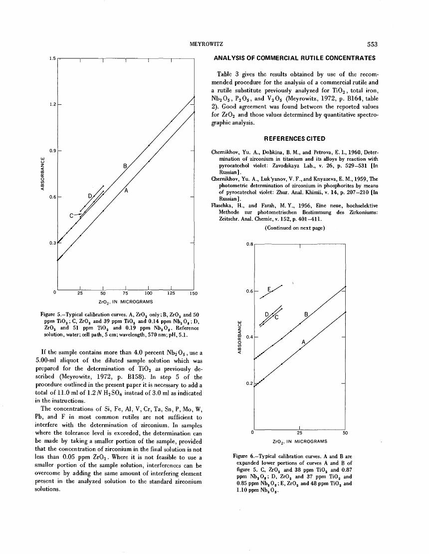
MEYROWITZ 553
ANALYSIS OF COMMERCIAL RUTILE CONCENTRATES
Table 3 gives the results obtained by use of the recom mended procedure for the analysis of a commercial rutile and a rutile substitute previously analyzed for Ti02 , total iron, Nb2 05 , P2 05 , and V2 05 (Meyrowitz, 1972, p. B164, table 2). Good agreement was found between the reported values for Zr02 and those values determined by quantitative spectre- graphic analysis.
REFERENCES CITED
Chernikhov, Yu. A., Dobkina, B. M., and Petrova, E. I., 1960, Deter mination of zirconium in titanium and its alloys by reaction with pyrocatechol violet: Zavodskaya Lab., v. 26, p. 529 531 [In Russian].
Chernikhov, Yu. A., Luk'yanov, V. F.,and Knyazeva, E. M., 1959, The photometric determination of zirconium in phosphorites by means of pyrocatechol violet: Zhur. Anal. Khimii, v. 14, p. 207 210 [In Russian].
Flaschka, H., and Farah, M. Y., 1956, Eine neue, hochselektive Methode zur photometrischen Bestimmung des Zirkoniums: Zeitschr. Anal. Chemie, v. 152, p. 401-411.
(Continued on next page)
25 50 75 100
ZrO2 . IN MICROGRAMS
125 150
Figure 5. Typical calibration curves. A, Zr0 2 only;B, Zr03 and 50 ppm Ti0 2 ; C, ZrO, and 39 ppm Ti03 and 0.14 ppm Nb2 0 $ ; D, Zr03 and 51 ppm Ti0 3 and 0.19 ppm Nba O s . Reference solution, water; cell path, 5 cm; wavelength, 570 nm; pH, 5.1.
If the sample contains more than 4.0 percent Nb2 05 , use a 5.00-ml aliquot of the diluted sample solution which was prepared for the determination of Ti02 as previously de scribed (Meyrowitz, 1972, p. B158). In step 5 of the procedure outlined in the present paper it is necessary to add a total of 11.0 ml of 1.2 JV H 2 S04 instead of 3.0 ml as indicated in the instructions.
The concentrations of Si, Fe, Al, V, Cr, Ta, Sn, P, Mo, W, Pb, and F in most common rutiles are not sufficient to interfere with the determination of zirconium. In samples where the tolerance level is exceeded, the determination can be made by taking a smaller portion of the sample, provided that the concentration of zirconium in the final solution is not less than 0.05 ppm Zr02 . Where it is not feasible to use a smaller portion of the sample solution, interferences can be overcome by adding the same amount of interfering element present in the analyzed solution to the standard zirconium solutions.
0.2
25 50
ZrO 2 , IN MICROGRAMS
Figure 6. Typical calibration curves. A and B are expanded lower portions of curves A and B of figure 5. C, Zr02 and 38 ppm TiO, and 0.87 ppm NbjO,; D, Zr0 3 and 37 ppm Ti0 3 and 0.85 ppm Nb3 0 s ; E, Zr03 and 48 ppm Ti0 3 and 1.10 ppm Nb3 03 .
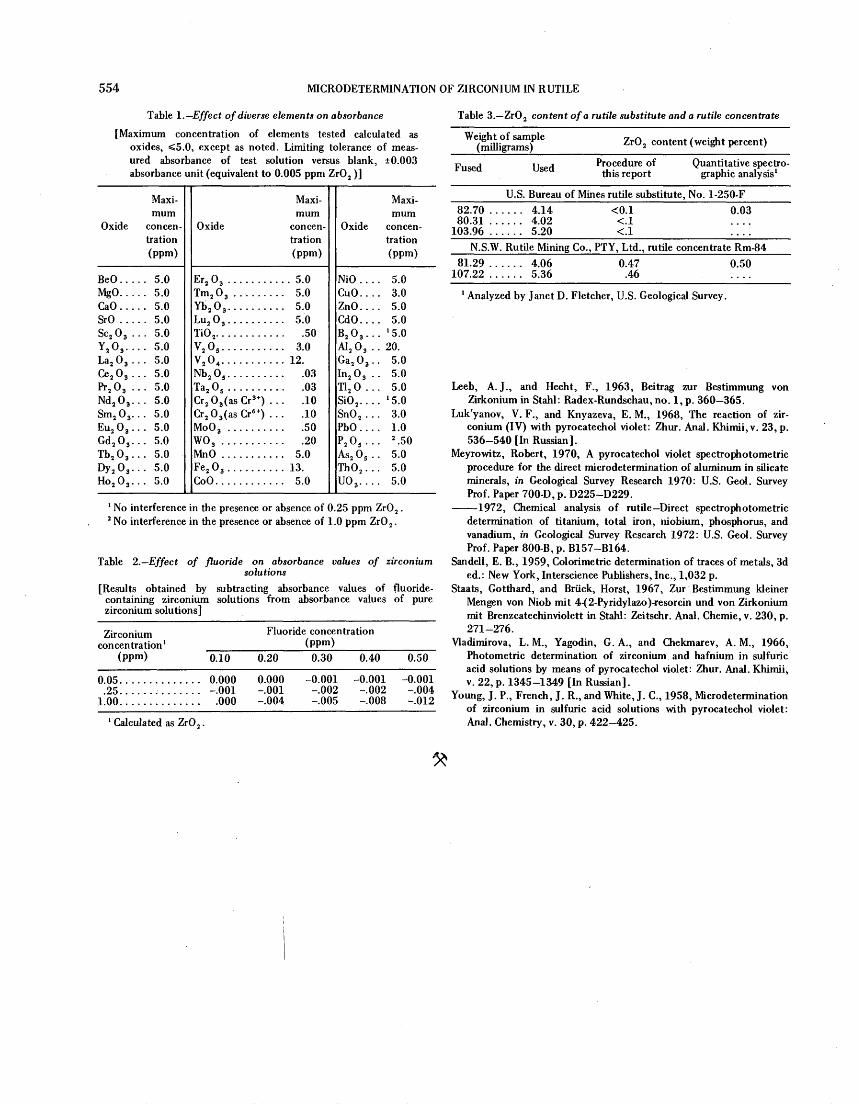
554 MICRODETERMINATION OF ZIRCONIUM IN RUTILE
Table 1. Effect of diverse elements on absorbance
[Maximum concentration of elements tested calculated as oxides, <5.0, except as noted. Limiting tolerance of meas ured absorbance of test solution versus blank, ±0.003 absorbance unit (equivalent to 0.005 ppm Zr0 2 )]
Table 3. Zr0 2 content of a rutile substitute and a rutile concentrate
Oxide
BeO . . .MgO. ..CaO...SrO . . .Sc2 0 3 .Y 0La2 0 3 .Ce OPr,0 3 .Nd2 0 3 . Sm2 0 3 . Eu2 0 3 .Gd 2 0 3 .Tb,0 3 .Dy 2 0 3 .Ho2 0 3 .
Maxi mum
concen tration (ppm)
. . 5.0. 5.0. 5.0
. . 5.0
. . 5.0. 5.0. 5.0
. . 5.0
. . 5.0. 5.0 . 5.0 . 5.0. 5.0. 5.0. 5.0. 5.0
Oxide
Er2 0 3 ........Tm2 0 3 .......VU f\Yb2 O 3 ... .....Lu2 0 3 .. ......TiOV 0V 0Nb2 0 s ........Ta A
Cr2 0 3 (asCr 3+) . Cr2 0 3 (asCr6+) . Mo0 3 ........W0 3 .........MnO .........FP OCoO....... ...
Maxi mum
concen tration (ppm)
.. 5.0
. 5.0
. 5.0
. 5.0. .50. 3.0. 12.. .03. .03. .10 . .10 . .50. .20. 5.0. 13.. 5.0
Oxide
NiO . . .CuO. . .ZnO...CdO...B r\ 2 O 3 . .Al O
Ga2 0 3 .In2 0 3 .
1 O
T12 0 . .Si0 2 . . . Sn0 2 . . PbO . . .P 0A« OTh02 . .U0 3 ...
Maxi mum
concen tration (ppm)
. 5.0
. 3.0
. 5.0
. 5.0
. '5.0
. 20.
. 5.0
. 5.0
. 5.0
. '5.0
. 3.0
. 1.0
. 2 .50
. 5.0
. 5.0
. 5.0
1 No interference in the presence or absence of 0.25 ppm ZrO,2 No interference in the presence or absence of 1.0 ppm Zr0 2 .
Table 2. Effect of fluoride on absorbance values of zirconiumsolutions
[Results obtained by subtracting absorbance values of fluoride- containing zirconium solutions from absorbance values of pure zirconium solutions]
Zirconium concentration 1
(ppm)
0.05...........25.. ........
1.00. .........
Fluoride concentration (ppm)
0.10
. ... 0.000
. ... -.001
. . . . .000
0.20
0.000 -.001 -.004
0.30
-0.001 -.002 -.005
0.40
-0.001 -.002 -.008
0.50
-0.001 -.004 -.012
Weight of sample (milligrams) Zr02 content (weight percent)
Fused Used Procedure of this report
Quantitative spectro- graphic analysis 1
U.S. Bureau of Mines rutile substitute, No. 1-250-F82.70 ...... 4.1480.31 ...... 4.02
103.96 ...... 5.20
0.03
N.S.W. Rutile Mining Co., PTY, Ltd., rutile concentrate Rm-8481.29 ...... 4.06 0.47 0.50
107.22 ...... 5.36 .46 ....
1 Analyzed by Janet D. Fletcher, U.S. Geological Survey.
1 Calculated as ZrO,
Leeb, A. J., and Hecht, F., 1963, Beitrag zur Bestimmung von Zirkonium in Stahl: Radex-Rundschau, no. 1, p. 360 365.
Luk'yanov, V. F., and Knyazeva, E. M., 1968, The reaction of zir conium (IV) with pyrocatechol violet: Zhur. Anal. Khimii, v. 23, p. 536-540 [In Russian].
Meyrowitz, Robert, 1970, A pyrocatechol violet spectrophotometric procedure for the direct microdetermination of aluminum in silicate minerals, in Geological Survey Research 1970: U.S. Geol. Survey Prof. Paper 700-D, p. D225-D229.
1972, Chemical analysis of rutile Direct spectrophotometric determination of titanium, total iron, niobium, phosphorus, and vanadium, in Geological Survey Research 1972: U.S. Geol. Survey Prof. Paper 800-B, p. B157-B164.
Sandell, E. B., 1959, Colorimetric determination of traces of metals, 3d ed.: New York, Interscience Publishers, Inc., 1,032 p.
Staats, Gotthard, and Briick, Horst, 1967, Zur Bestimmung kleiner Mengen von Niob mit 4-(2-Pyridylazo)*esorcin und von Zirkonium mit Brenzcatechinviolett in Stahl: Zeitschr. Anal. Chemie, v. 230, p. 271-276.
Yladimirova, L. M., Yagodin, G. A., and Chekmarev, A. M., 1966, Photometric determination of zirconium and hafnium in sulfuric acid solutions by means of pyrocatechol violet: Zhur. Anal. Khimii, v. 22, p. 1345-1349 [In Russian].
Young, J. P., French, J. R., and White, J. C., 1958, Microdetermination of zirconium in sulfuric acid solutions with pyrocatechol violet: Anal. Chemistry, v. 30, p. 422-425.

Jour. Research U.S. Geol. Survey Vol. l,No.5,Sept.-Oct. 1973, p. 566 658
By E. G. LILLIE and L. PAUL GREENLAND,
Washington, D.C.
Abstract. Samples are decomposed with hydrofluoric acid and perchloric acid in the presence of W 18 * tracer. Molybdenum is extracted from a hydrochloric acid solution. with tributyl phosphate. Tungsten is separated from most other elements by extraction of the a-benzoinoximate into chloroform. Stannous chloride in concentrated hydrochloric acid is used to strip tungsten and reduce it to W*5 . The amount of tungsten is determined spectrophotometrically after extrac tion as the thiocyanate complex into amyl alcohol. The correction for chemical losses is determined by counting W 18 '.
Many procedures for the spectrophotometric determination of tungsten with thiocyanate have been published (Affsprung and Murphy, 1964; Peng and Sandell, 1963; Fogg and others, 1970a, b, 1971). Fogg, Marriott, and Burns (1970a) have made an extensive study of these procedures. In rock analyses, where concentrations of tungsten are generally low, interfer ences and lack of sensitivity have presented difficulties. The numerous problems associated with thiocyanate methods (Hobart and Hurley, 1962) have led to procedures using the color formed with dithiol for the determination of tungsten in rocks (Quin and Brooks, 1972; Chan and Riley, 1967). Although sensitivity is often increased in these methods, interferences, especially from molybdenum, have been noted.
The method described in this paper gives a reliable tungsten thiocyanate color owing to the prior separation of tungsten from most other sample constituents. After removal of molybdenum, iron, and some other elements by extraction with tributyl phosphate from hydrochloric acid solution, tungsten is extracted with a-benzoinoxime into chloroform and then stripped and reduced to W* 5 with stannous chloride in concentrated hydrochloric acid. Tungsten in this virtually pure solution is reacted with thiocyanate and extracted into a small volume of amyl alcohol for the spectrophotometric determination. The selectivity of the separations of tungsten from other elements can be enhanced by accepting losses of tungsten at each separation stage; the fraction of tungsten finally recovered is determined by counting W 1 8 1 .
Acknowledgments. We are greatly indebted to E. Y. Camp bell for assistance with the analyses. We are grateful to B. L. Ingram and D. R. Norton for very helpful reviews of an earlier version of the manuscript.
REAGENTS AND APPARATUS
Aluminum chloride solution: Dissolve 20 g of A1C1 3 '6H2 0 crystals in300 ml of concentrated hydrochloric acid. Dilute to 1 liter withwater.
Tributyl phosphate (TBP) solution: Mix 200 ml of tributyl phosphatewith 200 ml of chloroform.
a-Benzoinoxime solution: Dissolve 4.0 g of a-benzoinoxime in 200 mlof ethanol. Prepare fresh daily.
Stannous chloride solution, concentrated: Dissolve 9.0 g ofSnClj-2H 2 0 in 200 ml of concentrated hydrochloric acid. Preparefresh daily.
Stannous chloride solution, dilute: Dilute 50 ml of concentratedstannous chloride solution to 200 ml with water. Prepare fresh daily.
Potassium thiocyanate solution: Dissolve 39 g of potassium thiocyanatein 100 ml of water. Prepare fresh weekly.
Hydrochloric acid, 6 M: Dilute 258 ml of concentrated hydrochloricacid to 500 ml with water.
Ethanol solution: Mix 50 ml of ethanol with 50 ml of 6 M hydrochloricacid.
Standard tungsten solution, 100 Mg W per ml: Dissolve 0.0897 g ofanalytical reagent grade Na 2 W0 4 '2HjO and 0.30 g of sodiumhydroxide in 500 ml of water.
Tracer solution: Commercially available W 8 ' was diluted with 2percent NaOH to obtain about 10,000 counts per minute from a0.01-ml aliquot. The specific activity was such that <0.1 jug W wasadded in the 0.01-ml aliquot.
Counting apparatus: A 3- by 3-in. Nal (Tl) detector coupled to asingle-channel analyzer gated to pass the 59-keV tungsten X-ray wasused to count W 8 '.
Extraction apparatus: Eighteen separatory funnels were placed in a rackunder a fume hood. An air stream was passed through a 1-mm ID glasscapillary tube inserted through the top of each funnel into the lowerphase. The tubes were connected to a compressed-air source byplastic tubing. After mixing, the tubes were removed from the liquidand the layers allowed to separate. This apparatus is faster, lesstedious, and just as efficient as manual or machine shaking andenables 18 samples to be analyzed per day.
ANALYTICAL METHOD
Chemical procedure
Transfer 0.5 g of sample (2 20 ppm W) into a Teflon beaker. Add 0.01 ml of the tracer solution. Prepare a counting standard for the samples at the same time by diluting 0.01 ml of tracer to 10 ml with water in a glass counting vial. To
555

556 SPECTROPHOTOMETRIC DETERMINATION, TUNGSTEN, ISOTOPE DILUTION
silicate samples, add 15 ml of concentrated hydrofluoric acid and 1 ml of concentrated perchloric acid and evaporate overnight on a hotplate at a surface temperature of about 120 C. To sulfide samples, add 5 ml of fuming nitric acid and evaporate to dryness on a hotplate before the addition of hydrofluoric and perchloric acids. Chemical losses from this point on may be ignored because of the final correction by counting W 1 81 .
Add 15 ml of aluminum chloride solution to dissolve the salts and heat gently if necessary. Do not overheat as the acid concentration at this point is important. Transfer the solution to a 60-ml separately funnel. Extract twice with 10 ml of TBP solution, discard the organic phases, and wash with 10 ml of chloroform.
Pipet aliquots of standard tungsten solution to cover the range of 1 10 /ig into 50-ml glass beakers. Add 0.01 ml of tracer solution and 15 ml of aluminum chloride solution. Mix and transfer to 60-ml separatory funnels. Prepare a counting standard for the standard solutions at the same time by diluting 0.01 ml of tracer to 10 ml with water in a glass counting vial.
Add 5 ml of a-benzoinoxime solution to both sample and standard solutions in the separatory funnels and mix well. Extract for 2 minutes with 7 ml of chloroform. Collect the organic phase in a 20-ml glass beaker and save. Add another 5 ml of a-benzoinoxime solution to the funnels and mix. Extract for 2 minutes with another 7 ml of chloroform and add the organic phase to that from the previous extraction. Discard the aqueous phase and transfer the collected organic phases to the separatory funnel. Wash with 10 ml of dilute stannous chloride solution. Collect the organic phase in the 20-ml beaker, discard the aqueous phase, and return the organic phase to the separatory funnel. Strip with 5 ml of concentrated stannous chloride solution and discard the organic phase. Wash twice with 5 ml of chloroform.
Transfer the aqueous phase to a 15-ml glass beaker and heat for 10 minutes on a hotplate at a surface temperature of about 100°C. Cool in an ice bath and transfer to the separatory funnel. Add 0.25 ml of potassium thiocyanate solution and extract with 3.0 ml of amyl alcohol. Discard the aqueous phase. Add 1.0 ml of ethanol solution to the funnel and mix.
Drain the solution into a 5-cra cell and measure the absorbance in a spectrophotometer at 405 nm against amyl alcohol.
Transfer the solution from the cell into a glass counting vial. Rinse_ the cell with a small quantity of ethanol and add the rinsings to the vial. Dilute the solution in the vial to 10 ml with ethanol.
Count the sample solutions, standard tungsten solutions, and the counting standards. Correct the observed counting rates for the background counting rate.
Calculations
The number of micrograms of tungsten in each standard tungsten solution extract, X, is calculated from the equation
R l
where mj is the number of micrograms of tungsten initially added and RI and R^ are the counting rates of the standard tungsten solution and the counting standard for the standard tungsten solution, respectively.
A calibration curve is prepared by plotting values of X against the absorbance of the standard tungsten solutions. The number of micrograms of tungsten in the final sample solution extract, m 2 , is determined by reference to the calibration curve.
The number of micrograms of tungsten present in the original sample, Y, is calculated from the equation
#4Y - mo ,
#3where R$ and ^4 are the counting rates of the final sample solution and of the counting standard for the sample solution, respectively.
RESULTS AND DISCUSSION
The proposed procedure relies on two separations to isolate tungsten from most other elements. The a-benzoinoxime extraction has been used previously to separate tungsten and molybdenum from most other elements (Peng and Sandell, 1963; Fogg and others, 1971). A method was sought that would eliminate molybdenum interference.
The extraction of many chloride complexes, including Mo+6 , by oxygenated solvents has been employed widely. Mo9 tracer was used to study the extraction of molybdenum from hydrochloric acid solutions with tributyl phosphate into xylene. Molybdenum was extracted to an extent greater than 95 percent from hydrochloric acid solutions in the range of 2.5 to 6.0 M into xylene solutions ranging from 20 to 50 volume percent in tributyl phosphate. Chloroform eventually was selected as a diluent for the tributyl phosphate for reasons of convenience; substitution of chloroform for xylene had no effect on the extraction of molybdenum.
The extraction of most elements with tributyl phosphate increases with hydrochloric acid concentration. It was found that if the hydrochloric acid concentration was adjusted to 3.6 M, .molybdenum could be removed with little loss of tungsten from the samples. As for pure standard solutions, as much as 28 percent of the tungsten present can be lost with each TBP extraction. For this reason, the TBP extractions are omitted for the standard solutions. With this separation, as much as 0.5 mg of molybdenum can be present with no apparent effect on the final color. When larger amounts are present, additional TBP extractions can be made. In addition to the removal of molybdenum, the TBP extraction removes most of the iron.
Large amounts of copper (>1.0 mg) or titanium (>1.5 mg) are partially extracted into chloroform with a-benzoinoxime. A blue-green color indicates the presence of copper. Copper
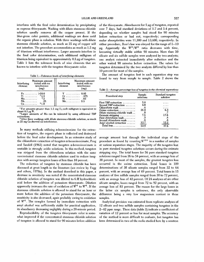
LILLIE AND GREENLAND 557
interferes with the final color determination by precipitating as cuprous thiocyanate. Washing with dilute stannous chloride solution usually removes all the copper present. If the blue-green color persists, additional washings are done until the organic phase is colorless. With three washings with dilute stannous chloride solution, as much as 25 mg of copper will not interfere. The procedure accommodates as much as 1.5 mg of titanium without interference. Larger amounts interfere in the final color determination, each additional milligram of titanium being equivalent to approximately 0.5 jug of tungsten. Table 1 lists the tolerance levels of nine elements that are known to interfere with the tungsten thiocyanate color.
Table 1. Tolerance levels of interfering elements
Interferingelement
Fe . . . .Ti ....Mo. ...Nb....Cu . . . .
Maximum amounttested with nointerference
(mg)
. . . . . >50.0
..... '1.52.5.25
.... 3 1.0
Interferingelement
vCr . . . .Ni . . . .Mn. . . .
Maximum amounttested with nointerference
(mg)
..... 0.05
..... .375
..... .02
..... 3.5
1 For amounts greater than 1.5 mg Ti, each milligram is equivalent to about 0.5 /ug W.
2 Larger amounts of Mo can be tolerated by using additional TBP extractions.
3 After three washings with dilute stannous chloride solution, as much as 25 mg Cu showed no interference.
In many methods utilizing a-benzoinoxime for the extrac tion of tungsten, the organic phase is collected and destroyed before the final color development. In an extensive study of the chloroform extraction of tungsten a-benzoinoximate, Peng and Sandell (1963) noted that tungsten a-benzoinoximate is unstable in strongly acidic solutions. In this method, tungsten was stripped from the chloroform solution with the same concentrated stannous chloride solution used to reduce tung sten with average tungsten losses of less than 10 percent.
The reduction of tungsten by stannous chloride has been discussed at great length in the literature (see review by Fogg and others, 1970a). In the method described in this paper, a decrease in sensitivity was noted if the concentrated stannous chloride solution of tungsten was diluted to 6 M hydrochloric acid before the addition of potassium thiocyanate. Dilution apparently increases the rate of oxidation of W1" 5 to Wf 6 . If the stannous chloride solution is allowed to stand for an hour or more before the addition of the potassium thiocyanate, the sensitivity is also decreased, again probably owing to oxidation of W1" 5 . The complex formed by immediate extraction with amyl alcohol was sufficiently stable for practical application, its absorbancy decreasing negligibly during a 20-minute period.
Reproducibility of the tungsten thiocyanate color is some what improved if the concentrated stannous chloride solution of tungsten is allowed to stand for 90 minutes before addition
of the thiocyanate. Absorbances for 5 jug of tungsten, repeated over 7 days, had standard deviations of 1.7 and 5.4 percent, depending on whether samples had stood for 90 minutes before extraction or had not, respectively; corresponding molar absorptivities were 11,300 and 13,400, respectively. In either procedure, Beer's law was obeyed for the range of 1 10 jug. Apparently the W* 5 /W6 ratio decreases with time, becoming virtually stable within 90 minutes. More than 50 silicate and six sulfide samples were analyzed by two analysts; one analyst extracted immediately after reduction and the other waited 90 minutes before extraction. The values for tungsten determined by the two analysts differed by less than 10 percent for most of the samples.
The amount of tungsten lost in each separation step was found to vary from sample to sample. Table 2 shoAvs the
Table 2. Average percentage loss of tungsten in the chemical separations
Procedural step
First TBP extraction .........Second TBP extraction .......
Dilute stannous chloride wash . .
Amyl alcohol extraction ......Total loss ................
Sample solutions
5.04.8
.421.0
.87.5
.3
.412.7^2 Q
Standard tungsten solution
6.3.7
17.6.4.4
12.237.6
average amount lost through the individual steps of the procedure as found by counting W 1 8 * in a number of samples at various separation stages. The majority of the tungsten lost in pure standard tungsten solutions occurs during the oximate stripping step. The total losses for 56 pure standard tungsten solutions ranged from 26 to 54 percent, with an average loss of 38 percent. In most of the samples, the greatest tungsten loss occurred in the oxime extraction. Total losses in 109 determinations of 38 silicate samples ranged from 32 to 64 percent, with an average loss of 49 percent. Total losses in 15 analyses of five sulfide samples ranged from 30 to 72 percent, with an average loss of 42 percent. Of 24 analyses of six other silicate samples, losses ranged from 72 to 92 percent, with an average loss of 83 percent. The reason for the large losses in the latter six samples is unknown, the only observable difference being a very low magnesium content in these samples.
Analytical precision was estimated from replicate analyses of 12 silicate and two sulfide samples containing tungsten in the 2 42 ppm range. These data (table 3) indicate a coefficient of variation of 12 percent or less for most samples. The accuracy of the method is more difficult to evaluate, but tungsten has been determined in two of the rocks studied here by a neutron
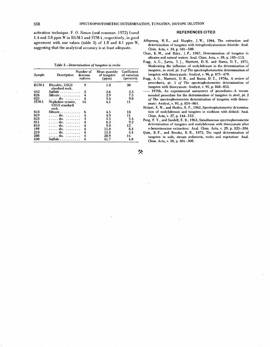
558 SPECTROPHOTOMETRIC DETERMINATION, TUNGSTEN, ISOTOPE DILUTION
activation technique. F. 0. Simon (oral commun. 1972) found 1.4 and 3.8 ppm W in RGM-1 and STM-1, respectively, in good agreement with our values (table 3) of 1.8 and 4.1 ppm W, suggesting that the analytical accuracy is at least adequate.
Table 3. Determination of tungsten in rocks
Sample
RGM-1
432 824 822 STM-1
818 819 823 811 810 199 210 208 430
Number of Description determi
nations
Rhyolite, USGS standard rock.
Silicate ............... do. .......Nepheline syenite,
USGS standard rock.
..... do. .......
..... do. .......
..... do. .......
..... do. .......
..... do. .......
..... do. .......
..... do. .......Sulfide ..........
9
. 3
. 44
14
. 6
. 4
. 34 4 44
. 4
. 4
Mean quantity of tungsten
(ppm)
1.8
2.6 2.9 3.4 4.1
4.5 4.9 5.5 6.2 9.0
11.0 15.3 28.9 41.7
Coefficient of variation (percent)
30
2.3 7.5 9.8
11
18 11
5.4 9.2
12 8.3 4.4
14 4.0
REFERENCES CITED
Affsprung, H. E., and Murphy, J. W., 1964, The extraction and determination of tungsten with tetraphenlyarsonium chloride: Anal. Chim. Acta, v. 30, p. 501-508.
Chan, K. M., and Riley, J. P., 1967, Determination of tungsten in silicates and natural waters: Anal. Chim. Acta, v. 39, p. 103 113.
Fogg, A. G., Jarvis, T. J., Marriott, D. R. and Burns, D. T., 1971, Moderating the influence of molybdenum in the determination of tungsten, in steel, pt. 3 of The spectrophotometric determination of tungsten with thiocyanate: Analyst, v. 96, p. 475 479.
Fogg, A. G., Marriott, D. R., and Burns, D. T., 1970a, A review of procedures, pt. 1 of The spectrophotometric determination of tungsten with thiocyanate: Analyst, v. 95, p. 848 853.
1970b, An experimental assessment of procedures A recom mended procedure for the determination of tungsten in steel, pt. 2 of The spectrophotometric determination of tungsten with thiocy anate: Analyst, v. 95, p. 854-861.
Hobart, E. W., and Hurley, E. P., 1962, Spectrophotometric determina tion of molybdenum and tungsten in niobium with dithiol: Anal. Chim. Acta, v. 27, p. 144-152.
Peng, P. Y., and Sandell, E. B., 1963, Simultaneous spectrophotometric determination of tungsten and molybdenum with thiocyanate after a-benzoinoxime extraction: Anal. Chim. Acta, v. 29, p. 325 334.
Quin, B. F., and Brooks, R. R., 1972, The rapid determination of tungsten in soils, stream sediments, rocks and vegetation: Anal. Chim. Acta, v. 58, p. 301-309.

Jour. Research U.S. Geol. Survey Vol. 1, No. 5 , Sept.-Oct. 1973, p. 559-562
SPECTROCHEMICAL COMPUTER ANALYSIS- ARGON-OXYGEN D-C ARC METHOD FOR SILICATE ROCKS
By A. F. DORRZAPF, JR., Washington, D.C.
Abstract. Use of an argon-oxygen atmosphere eliminates the inter ference of cyanogen bands with many sensitive analytical lines. The jet-controlled atmosphere also improves the stability of the arc. These procedural changes, coupled with computerized analysis of the spectra, result in increased detectability, precision, and speed as compared to the former visual semiquantitative technique.
Complete spectrochemical analysis of geologic materials by a recording system and computer was developed by Helz, Walthall, and Herman (1969). There has been a concerted effort in the U.S. Geological Survey laboratories since then to improve and extend the capability of this method. The improved system, the procedural part of which is described in this paper, is now in routine service.
Basic changes in the recording system have been described by Helz (1973). The previous system used two 102- by 254-mm (4- by 10-inch) plates to cover the entire wavelength range. Two recordings were, therefore, required for each sample spectrum. This procedure, moreover, necessitated fiducial lines for each plate as well as massive computer storage for a complete analysis. The conversion to 102- by 508-mm (4- by 20-inch) plates allows continuous recording of a spectrum from 2300 to 4700 A, uses only two fiducial lines, simplifies computer processing, and reduces storage requirements.
Although the conversion to 508-mm plates provided contin uity of recording, the cyanogen band region (3500 4216 A) was still of limited use for analyses. The intensity of these bands was reduced considerably by use of an argon-oxygen atmosphere during excitation. An additional advantage of this atmosphere is better arc control.
Acknowledgments. The author gratefully acknowledges the guidance and assistance of Armin W. Helz and the cooperation and assistance of other colleagues, in particular Sol Berman and Frank G. Walthall.
EXPERIMENTAL METHOD
The basic guideline for this work was to keep the method simple, rapid, and as sensitive for trace and minor elements as the semiquantitative method of Myers, Havens, and Dunton
(1961). To eliminate cyanogen bands, an atmosphere can be introduced around the electrodes by using some type of jet. The jet designed by Helz (1964) was preferred over the Stallwood model (Stallwood, 1954) because no glass dome is required on the Helz jet, thus eliminating cleaning of the dome between exposures. Various atmospheres have been used to eliminate cyanogen bands (Thiers, 1953; Thiers and Vallee, 1957; Shaw and others, 1958). After investigating many of these gases and combinations of argon and oxygen, we chose a mixture of 70 percent argon and 30 percent oxygen at a flow rate .of 6.6 1/min.
It was necessary to increase the size of the sample used in the semiquantitative procedure from 10 mg of sample and 20 mg of graphite to 15 mg of sample and 30 mg of graphite to maintain the desired sensitivity for all elements. In addition, an increase of the initial burning time, at 5 amp, from 10 to 20 sec maintains the sensitivity for volatile elements. The details of excitation and other spectrographic conditions follow:
Electrodes: Cathode, ASTM type C-6, 2 in. long; anode, 54-in. diamthin-walled graphite (Ultra No. 3170).
Electrode charge: 15 mg sample + 30 mg graphite (type UCP-2/200mesh).
Spectrograph: 3.4 m Ebert design (Mark III). Power source: 325 v open circuit d-c arc, resistance controlled. Excitation: 15 amp d-c arc set with empty graphite electrodes. Arc gap: 4 mm, maintained throughout burn. Exposure: 20 sec at 5 amp followed by 130 sec at 15 amp, continuous
burn. Atmosphere: 70 percent argon + 30 percent oxygen; 6.6 1/min flow rate
with top of Helz jet nozzle 2 mm below top of electrode. Wavelength range: 2300-4700 A; first order. Grating: 600 groove/mm; 5 A/mm reciprocal linear dispersion. Slit: 25 MT» wide and 2 mm high. Filter: 47-percent transmission neutral-density filter. Illumination: Arc image focused on collimator by 450-mm focal-length
lens at slit.Mask at collimator: 1.8 cm. Emulsion: Kodak HI-0 (102- by 508-mm plates). Processing: Kodak D-19 developer, 3/4 min at 20°C; Kodak indicator
stop bath, 30 sec; Kodak fixer, 8 min; wash, 20 30 min at 20 C; anddry with warm air for 20 min.
Six-step standards are prepared as described by Myers, Havens, and Dunton (1961). All standards and samples are weighed, mixed with graphite, and loaded into the electrode in
559

560 SPECTROCHEMICAL COMPUTER ANALYSIS-ARGON-OXYGEN D-C ARC METHOD
Table 1. Spectral lines used in spectrochemical computer analysis, listed in order of sensitivity
Ele- Wavelength ment (angstroms)
Ag .
Al .
As .
Au .
B ..Ba .
Be .
Bi .
Ca .
Cd .
Ce .
Co .
Cr .
Cs .
Cu .
Dy .
Er .
Eu .
Fe .
Ga .
Gd .
Ge .
Hf .
Hg .
Ho .
. 3280.6833382.891
. 2660.3932378.4082669.166
. 2860.4522349.842370.772369.67
. 2675.952427.953122.781
. 2496.778
. 4554.0424130.6643071.591
. 2348.6103321.3433321.086
. 3067.7162897.9753024.635
. 2997.3142721.6453274.661
. 3261.0573466.201
. 4165.6063201.714
. 3453.5053449.1703412.633
. 3593.4884254.3463024.3502843.2522731.908
. 4555.3554593.177
. 3247.5403273.9622824.369
. 3407.804211.7193319.887
. 3230.5853220.730
. 4129.7374205.0462906.6762813.952727.780
. 3175.447 2391.474 2385.007
. 2943.637 2944.175
. 3549.365 3331.388
. 2651.1782651.5753269.494
. 2916.4813109.1172866.373
. 2536.5193131.833
. 3456.003398.98
Concentration limits
(percent)
0.000010- 0.000681.000010- .00100
0.0316 - 0.464.215 - 2.15
2.15 -31.60.0100 - 1.00.316 - 1.00.215 -10.0.215 -10.0
0.000681- 0.0147.00100 - .0681.00215 - .100
0.00100 - 0.02150.000100- 0.00147.00147 - .0464.0100 - .215
0.000100- 0.00464.000100- .0100.000215- .0147
0.000100- 0.0100.00215 - .100.0100 - .215
0.0681 - 3.16.464 -31.6
1.00 -31.60.00147 - 0.0464.00464 - .0681
0.00200 - 0.136.00431 - .431
0.000100- 0.00464.000100- .0215.000464- .0215
0.000100- 0.00100.000100- .00215.000464- .0681.000464- .100.0100 - .681
0.316 - 1.471.00 - 4.640.000100- 0.000681.000215- .00100.00464 - .1000.000316- 0.0316.000316- .0147.00100 - .100
0.000215- 0.0316.000681- .100
0.000100- 0.00316.000100- .00316.000681- .100.00100 - .100.00316 - .100
0.0506 - 5.06 .506 -23.5
1 09 23.5 0.000215- 0.00316 .00147 - .100
0.000316- 0.0215 .00215 - .100
0.000100- 0.0215.00464 - .0681.00464 - .0681
0.00100 - 0.464.00464 - .681.00681 - .681
0.0147 - 2.15.464 - 4.64
0.000100- 0.00681.000316- .0147
Ele ment
In .
Ir ..
K ..
La .Li .
Lu .Mg .
Mn .
Mo .
Na .
Nb .
Nd .Ni .
Os .
P ..Pb .
Pd .
Pr .
Pt .
Rb .
Re .
Rh .
Wavelength (angstroms)
. 4511.3233039.356
. 3220.7802849.725
. 4044.1404047.2013446.372
. 3245.120
. 3232.614273.283985.79
. 2911.39
. 2779.8342776.6902782.9742781.4173336.6802798.063329.9302936.5372938.5384571.15
. 2798.2712801.0642949.2054502.2203070.2663629.7412914.6032626.6402713.3312387.02
. 3864.1103170.3473193.9732816.154
. 3302.3233302.9882853.0312852.828
. 3163.4023194.977
. 4303.573
. 3492.9563101.8792943.914
. 3301.5592909.061
. 2554.93
. 2833.0692663.1662873.3162393.794
. 3404.580 3242.703 3516.943
. 3908.431 4222.98 3121.571
. 2997.9672659.4542830.295
. 3591.593348.72
. 3460.473464.722
. 3434.8933692.3573396.85
Concentration limits
(percent)
0.000464- 0.00681.000464- .0147
0.000681- 0.100.00464 - .215
0.0681 - 0.681.147 - 1.00
1.00 -10.00.00147 - 0.1470.00316 - 0.215.316 - 1.47.464 - 4.64
0.000316- 0.04640.00215 - 0.0681.00215 - .215.00215 - .316.00464 - .316.00464 - .316.00681 - .681.0100 - 2.15.0316 - 2.15.100 - 6.81
1.47 -30.00.000100- 0.0100.000100- .0147.000316- .0316.00681 - .681.00681 - 1.00.0147 - 1.00.0147 - 1.47.215 - 4.64.681 -10.0
4.64 -46.40.000100- 0.00215.000147- .0147.000215- .0147.00215 - .100
0.00464 - 0.147.00681 - .316.0681 - 4.64.215 - 6.810.000215- 0.0681.000464- .100
0.00147 - 0.04640.000100- 0.00215.000464- .0316.00147 - .100
0.000100- 0.100.00215 - .147
0.0464 - 4.640.000100- 0.0681.00681 - .100.0147 - .100.0681 - 4.64
0.000022- 0.00147 .000068- .00464 .000215- .00681
0.000215- 0.00681 .00147 - .0316 .0316 - .100
0.000681- 0.0464.000681- .0681.00215 - .100
1.47 -10.03.16 -10.00.00100 - 0.0464.00215 - .0681
0.000010- 0.00147.000100- .00147.000147- .00464
Ele ment
Ru .
Sb .
Sc .
Si .
Sm .
Sn .
Sr .
Ta .
Tb .
Te .Th .
Ti .
Tl .
Tm.
U ..
V ..
W .
Y ..
Yb .
Zn .
Zr .
Wavelength (angstroms)
3502.5243462.040
. 3498.9423436.7372988.948
. 2598.0622877.9153267.5022670.6432445.5152383.63
. 3911.8104246.8293353.734
. 2519.2072987.6482452.1362577.13
. 4296.7503408.668
. 3175.0193034.1212839.9892863.327
. 4077.7144607.3313464.4574161.7962931.8302569.4692428.095
. 3311.1622714.674
. 3293.074278.51
. 2385.76
. 4116.7184069.2102837.2992870.413
. 3199.9153186.4542641.0992644.2642679.926
. 3775.723519.242767.873529.433229.75QAfio on
. «J*i!vJfc*.fcivF
40Q4, 1ftTP\/;7T?« JL\J
. 4244.372 3270.124 2865.679
. 3102.299 3183.406 3134.931
. 4008.7532896.4462946.981
. 3327.8753195.615
. 3987.9943464.370
. 3345.0203345.572
. 3279.265
Concentration limits
(percent)
0.000215- 0.00681.000681- .0147
0.000046- 0.00464.000100- .0100.00147 - .147
0.00681 - 0.100.00681 - .147.0100 - .316.100 - 2.15.215 - 6.81
1.00 - 6.810.000100- 0.00215.000100- .00316.000100- .00681
0.00316 - 0.100.0147 - .681.100 -14.7
2.15 -34.30.000464- 0.00464.00316 - .100
0.000316- 0.0147.000316- .0215.00100 - .0215.00681 - .0316
0.000046- 0.000215.000100- .00215.00147 - .0464.00464 - .147.0681 - 6.81
1.00 -46.42.15 -46.40.0147 - 1.00.0316 - 1.00
0.00147 - 0.100.00464 - .100
0.0316 - 1.000.00215 - 0.215.0100 - .316.0100 - .464.0147 - .681
0.000464- 0.0464.000464- .100.0100 - .316.0681 - .681.100 - 6.810.000316- 0.00681.00147 - .0147.00147 - .100.00681 - .100.100 - .681
0.000316- 0.0100.000464- .01470.0215 - 0.464 .0316 - 1.00 .0681 - 1.00
0.000147- 0.0100 .000147- .0215 .00147 - .100
0.00100 - 0.0681.00215 - .464.00464 - .464
0.000316- 0.0215.000316- .0464
0.000068- 0.00147.000681- .0100
0.00147 - 0.0464.00100 - .316
0.000316- 0.0681

DORRZAPF 561
the usual manner, final tamping of the sample being accom plished with a special tamper (fig. 1).
Figure 1. Aluminum alloy tamper. This tamper provides more surface area than a flat-end tamper and facilitates the escape of gases from the sample with minimum sample loss.
Special efforts are made to assure identical conditions in the arcing of all samples and standards. The jaws in the arc stand were modified by the addition of a simple stop to permit each electrode to be grasped at the same point and cooled to the same extent during each burn.
Because the electrodes are being consumed more rapidly in the gas flow than in air, they require more frequent adjust ment to maintain the arc gap. Some sample types form beads during the latter part of the arcing. The size of the bead is a function not only of the composition of the sample but of its mixing with the graphite; the better the mixing, the smaller the bead. Loss of a bead can cause low results for some of the major elements (Si, Al, Fe, and Ca). By controlling mixing and burning conditions for samples and standards, however, the results for these elements usually fall within the precision and
accuracy of the method.Each spectrum contains two cadmium reference lines super
imposed with a lamp and mask assembly as described by Helz (1973), who also described the photoprocessing equipment for the 508-mm plates and the densitometer-recorder system.
Plate calibration, line finding, construction of analytical curves, and calculations are performed by the computer and will be described in detail in a subsequent paper by Walthall (1973).
RESULTS AND DISCUSSION
Detection limits and useful concentration ranges for individ ual lines of 68 elements determined with this technique are given in table 1. These limits and ranges are a function of the analytical lines chosen, exposure, interferences, and limitations of the recording system. A third significant figure is used solely for programing convenience. Of the 206 lines, 27 occur in the cyanogen band region and include the most sensitive lines for Ce, Cr, Eu, Gd, K, Mo, Pr, Rb, Sc, Sr, Th, Tl, W, and Yb. The detection limits for most elements are equal to or better than those obtained by the visual semiquantitative method. We are programing the computer for correcting interferences; many of the limits and ranges will be changed as a result.
A detailed study of the precision of this method, using a variety of sample types, has been made in a study of twelve
U.S. Geological Survey standard rocks by F. G. Walthall, A. F. Dorrzapf Jr., and F. J. Flanagan (unpub. data). The precision is within the range of +50 to -30 percent of the amount present, as expected of a semiquantitative method, and approaches ±10 15 percent for many elements, as normally expected of a quantitative method. Data on standard diabase W-l from this study are given in table 2.
Table 2. Standard deviation and coefficient of variation for standard diabase W-l
[From F. G. Walthall, A. F. Dorrzapf, Jr., and F. J. Flanagan, unpub. data]
Element Average Standard concentration 1 deviation 2
Coefficient of variation 3
Percent
Si .......Al .......Fe .......Mg.......Ca.......K .......Ti .......Mn.......
...... 27.7
...... 9.77
...... 9.29
...... 6.13
...... 8.67
...... .652
...... .727
...... .186
2.3 1.2 .20 .15 .45 .096 .048 .006
8.30 12.3
2.15 2.45 5.19
14.7 6.60 3.23
Parts per million
Ba .......Co .......Cr .......Ga .......La .......Nb.......Ni .......Pb .......Sr .......Y .......Yb.......Zn .......Zr .......
141...... 53.1...... 157...... 21.2...... 17.8...... 7.1...... 86.4...... 7.26...... 248...... 26.4...... 4.23...... 147...... 142
9.7 2.7 6.7 1.2 2.1 2.5 8.7
.73 15.6
2.3 .24
4.9 16.3
6.88 5.08 4.27 5.66
11.8 35.2 10.1 10.1 6.29 8.71 5.67 3.33
11.5
1 Average of six determinations; three bottles, two portions of each.2 Square root of the error mean square calculated in the analyses of
variance.3 Coefficient of variation equals standard deviation times 100 divided
by average concentration.
Despite marked improvements in spectrochemical methods in the last several decades, the determinations of the major constituents of a rock have been generally within the province of chemical methods. In the hope that this computer-based method might yield data for the major constituents that would be comparable to chemical determinations, duplicate portions of 20 samples have been analyzed randomly. These samples had been previously analyzed chemically.
To determine if the differences between the chemical and spectrographic data were significant, the t test in the form
J/7T t = as shown by Youden (1951, p. 28) was used. In the
sd
summary shown in table 3, the chemical data were assumed tobe correct, and the differences chemical minus spectro graphic were converted to percent of the chemical data. The average difference, d, and the standard deviation of the

562 SPECTROCHEMICAL COMPUTER ANALYSIS-ARGON-OXY3EN D-C ARC METHOD
Table 3. Comparison of chemical and spectrographic data for 20 samples
[d is the average difference in percent from chemical data, n is number of pairs, t is the t distribution with n-1 degrees of freedom. A positive difference indicates that values of chemical data are greater. NS indicates that the average difference is not significant at t0 9 5 ]
Oxide
SiO......A1 2 5 3 ... Fe 2 0 3 ... MgOCaO. . . . .K 2 0....TiOp nMnO
Range of oxide
data (percent)
. 45.1 -76.4
. 10.9 -22.6
. 1.46-16.8 .06 13.2.34-12.7.09- 6.2309 2 67
.01 .99
.03 .24
d
+11.3+19.8
+1.82 +16.1-2.92+2.19
+9d 91ft Q
-11.8
2020 20 90?,016901090
Calculated
3.893.95
.812 NS 9 35
.434 NS
.460 NS3.831 ftQ NS9 7Q
t
From tables
2.092.09 2.09 2.092.092.132.099 962.09
differences, sj, were calculated from these n differences. The tests showed that the paired differences for Fe2 03 , CaO, K2 0, and P2 05 were not significant and both methods may be said to yield comparable data. Further refinements are necessary for the determination of the remaining oxides but especially for Si02 , A12 03, and Ti0 2 for which the differences are significant at greater than tQ -99 .
REFERENCES CITED
Helz, A. W., 1964, A gas jet for d-c arc spectoscopy: Art. 159 in U.S.Geol. Survey Prof. Paper 475-D, p. D176-D178.
1973, Spectrochemical computer analysis instrumentation: U.S.Geol. Survey Jour. Research, v. 1, no. 4, p. 475 482.
Helz, A. W., Walthall, F. G., and Herman, Sol, 1969, Computer analysisof photographed optical emission spectra: Appl. Spectroscopy, v.23, no. 5, p. 508-518.
Myers, A. T., Havens, R. G., and Dunton, P. J., 1961, A spectrochemi-cal method for the semiquantitative analysis of rocks, minerals, andores: U.S. Geol. Survey Bull. 1084-1, p. 207-229.
Shaw, D. M., Wickremasinghe, 0., and Yip, C., 1958, A simple devicefor the spectrochemical analysis of minerals in an inert atmosphereusing the Stallwood jet: Spectrochim. Acta, v. 13, p. 197 201.
Stallwood, B. J., 1954, Air-cooled electrodes for the spectrochemicalanalysis of powders: Optical Soc. America Jour., v. 44, p. 171.
Thiers, R. E., 1953, The advantages of controlled atmospheres for arcspectroscopy: Appl. Spectroscopy, v. 7, p. 157 163.
Thiers, R. E., and Vallee, B. L., 1957, The effect of noble gases on thecharacteristics of the d-c arc, in Colloquim SpectroscopicumInternationale, VI, Amsterdam, 1956, Proc.: London, PergamonPress, p. 179-185.
Walthall, F. G., 1973, Spectrochemical computer analysis Programdescription: U.S. Geol. Survey Jour. Research, v. 1, no. 6 (In press.)
Youden, W. J., 1951, Statistical methods for chemists: New York, JohnWiley and Sons, Inc., 126 p.
Jour. Research U.S. Geol. Survey Vol. l,No.5, Sept.-Oct. 1973, p. 563 5 67
BATHYMETRY OF THE CONTINENTAL MARGIN OFF LIBERIA, WEST AFRICA
By JAMES M. ROBB, JOHN SCHLEE,
and JOHN C. BEHRENDT, Falmouth, Mass.
Abstract. A bathymetric map based on new data allows examination of geomorphic features on the narrow continental margin off Liberia. The continental shelf in this region is relatively flat and featureless. The northwestern part of the continental slope, off Monrovia and Cape Mount, shows complex slump features and two submarine valleys. The central part of the slope is smoother, apparently as a result of progradation. The southeastern part of the slope, near Cape Palmas, is crossed oblique to the shoreline by a structural valley that has been modified by large slumps or landslides. This valley may be the termination, at the continental margin, of an oceanic fracture zone. The major slumplike features of the Liberian continental margin appear to be surface manifestations of deep faulting which has been partially masked by sedimentation.
A bathymetric contour map derived from more detailed data than were previously available has been prepared as part of geophysical studies of the continental margin of Liberia (Schlee and others, 1972; Schlee, 1972).
Reconnaissance bathymetric maps that include the conti nental margin off Liberia have been produced by the Association des Services Geblogiques Africains (1968), Somers (1969), and Uchupi (1971). Rancurel (1965) published a map of the continental shelf of Liberia and the Ivory Coast, which included areas of sediment cover, rock outcrop, and biogenic features. Part of the eastern end of the Liberian continental margin is included in a contour map by Arens and others(1971). Part of the northwestern end is discussed by Egloff(1972). Geologic studies of the narrow continental margin of Liberia have been published by Behrendt and Wotorson (1970) and Templeton (1971).
METHODS
The survey was made aboard the RV Unitedgeo I in November 1971 by the U.S. Geological Survey in cooperation with the Liberian Geological Survey; it was funded by the National Science Foundation under the International Decade of Ocean Exploration (IDOE) (Schlee and others, 1972). Depths were sounded with a 3.5-kHz transducer system and corrected for sound speed variations (Matthews, 1939). A
satellite system aboard the RV Unitedgeo I gave fixes at about 2-hour intervals accurate to about 180 m. These were supplemented by Doppler sonar and radar. Navigational accuracy was excellent. Comparison of depths at track crossings indicates positional error of less than 1 km.
Locations of sounding tracks are shown in figure 1. Data from USNS Kane (Lowrie and Escowitz, 1969) were included (6.5 km or greater sounding interval). In addition, a contour map and bathymetric data from R. L. McMaster (oral com- mun., 1972) were consulted. The curve in the edge of the continental shelf at long 8°20' W. was taken from Rancurel (1965).
DISCUSSION
The continental margin off Liberia has been divided into three sectors characterized by different types of submarine topography (fig. 1): (1) a northwest sector, Cape Mount to Buchanan; (2) a central sector, Buchanan to east of Greenville; and (3) a southeast sector, east of Greenville to Harper.
The northwest and southeast sectors of the margin are narrow, and the slope is topographically complex. The central sector is wider and smoother. Figure 2 shows selected profiles that typify these sectors.
In the northwest sector (fig. 2, profiles 3, 6, and 12) the continental shelf is about 25 km wide. The continental slope is about 60 km wide, has an average slope of about 3 , and is characterized by many features that resemble slump and landslide scars and rubble. At least two large submarine valleys cut the slope, off the St. Paul and Farmington Rivers. The upper slope between Cape Mount and Monrovia is extremely rough; it contains many small valleys averaging about 170 m in depth and spaced at intervals of about 3 km (R. L. McMaster, oral commun., 1972). These valleys are too small to contour with the present data density or at this scale.
In contrast, off Greenville in the central sector, the surface of the slope is much smoother; the slope has smaller slump scars and no valleys. The smooth regular surface of the upper slope suggests depositional progradation. The continental shelf in the central sector is about 45 km wide; the continental slope is
563
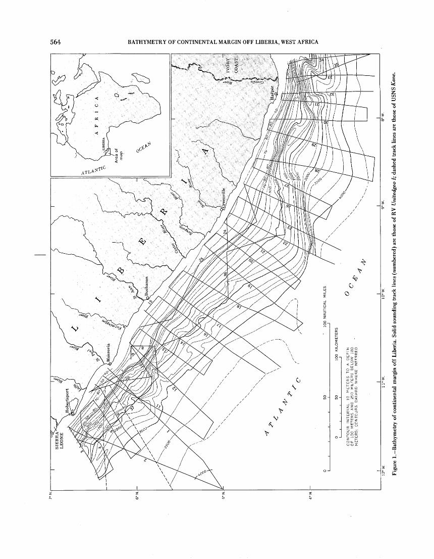
564 BATHYMETRY OF CONTINENTAL MARGIN OFF LIBERIA, WEST AFRICA

ID
CENTRAL
I I I \l I I I I I I I ll I I I I I I I II I I I I I I I
I<3N3HH3a QNV '331HDS '*

566 BATHYMETRY OF CONTINENTAL MARGIN OFF LIBERIA, WEST AFRICA
about 95 km wide and has a slope of about 1.8° (fig. 2, profiles 17, 19, and 23). A steeper (to 15°) section near the base of the slope shows a linear, easterly trend, subparallel with a valley farther east above the continental slope.
Off Harper, in the southeast sector, the continental shelf is about 20 km wide. The continental slope is about 75 km wide, has an average slope of about 3° but has slopes locally of 10 to 15° (fig. 2, profiles 29, 32, and 34). This sector is cut by a large valley trending southwest, oblique to the trend of the continental slope. We interpret this valley as the continuation, or termination at the continental margin, of the oceanic St. Paul fracture zone (Heezen and Tharp, 1965, p. 94). Seismic reflection profiles (Schlee, 1972) distinctly show a ridge in the subsurface below the southwestern wall of the valley. The valley is apparently filled by a large slump at its western end. It is probably analogous to a similar subsurface ridge-and- valley structure which Fail and others (1970), Arens and others (1971), and LePichon and Hayes (1971) described off Cape Three Points and the Ivory Coast, and which they related to the Romanche fracture zone. Uchupi (1971) showed a double ridge extending southwest from Cape Palmas into the ocean basin.
The surface of the continental shelf is generally flat and featureless along the whole coastline of Liberia, although irregularities are found in the very nearshore area (R. L. McMaster, oral commun., 1972). Small, irregular highs of 2 or 3 m relief occur on the middle and outer shelf in a few places but are more frequent southeast of long 8° 20' W. These highs are probably rock outcrops (Rancurel, 1965). A persistent zone of irregular topography occurs at depths of 80 120 m on the shelf edge (fig. 3). Such bands are common along much of the West African margin and are probably relict strandlines and coralline or algal growths formed during lower stands of sea level (McMaster and others, 1970).
The depth to the shelf break ranges from 100 to 150 m. In the northwest sector, this depth is relatively constant at about 134 m. In the central sector the break is difficult to pick, as the transition from shelf to slope is smoothly rounded. In the southeast sector, where the shelf break occurs at depths of 100 150 m, the shallower depths are at the heads of steep slopes which appear to have resulted from slumping.
By aeromagnetic methods, Behrendt and Wotorson (1970) have located several basement faults under the continental shelf. Depth to the shelf break changes from 134 to 115 m across one of these faults southeast of Monrovia (at lat 5 54' N., long 10°46' W.) and is consistent with their interpretation of downfaulting to the southwest. As these faults are thought to be Cretaceous in age, a surface trace may be evidence of rejuvenated faulting.
Slump features and valleys of the continental slope appear to relate closely to subsurface faulting observed in seismic reflection profiles (Schlee, 1972) and in some instances may represent fault scarps. Features of the submarine topography appear to be surface manifestations of complex subsiding
blocks along the margin of the continent, although sedimenta tion has masked their outlines.
SUMMARY
The continental shelf off Liberia is narrow and relatively flat, marked by topographic relief only along old strandlines near the shelf break, and in a few other places where probable rock outcrops occur.
The continental slope is topographically more complex. Off the northwestern coast of Liberia it shows slumplike features and two submarine valleys. Off the central part of the country, the continental slope is smoother; its upper part may be a progradational surface. The southeastern part of the slope also shows slumplike features and contains a large structurally controlled valley which is probably an extension of the oceanic St. Paul fracture zone. The geomorphic features of the continental slope appear to be closely related to basement faulting.
REFERENCES CITED
Arens, G., Delteil, J. R., Valery, P., Damotte, B., Montadert, L., and Patriat, P., 1971, The continental margin off the Ivory Coast and Ghana, in Delany, F. M., ed., The geology of the east Atlantic continental margin; 4, Africa: [Great Britain] Inst. Geol. Sci. Rept. 70/16, p. 61-78.
Association des Services Geologiques Africains, 1968, International tectonic map of Africa, sheet 4: Paris, UNESCO, scale 1:5,000,000.
Behrendt, J. C., and Wotorson, C. S., 1970, Aeromagnetic and gravity investigations of the coastal area and continental shelf of Liberia, West Africa, and their relation to continental drift: Geol. Soc. America Bull., v. 81, no. 12, p. 3563-3574.
Egloff, Julius, 1972, Morphology of ocean basin seaward of northwest Africa; Canary Islands to Monrovia, Liberia: Am. Assoc. Petroleum Geologists Bull., v. 56, no. 4, p. 694-706.
Fail, J. P., Montadert, L., Delteil, J. R., Valery, P., Patriat, P., and Schlich, R., 1970, Prolongation des zones de fractures de I'oc&n Atlantique dans le Golfe de Guinee: Earth and Planetary Sci. Letters, v. 7, no. 5, p. 413-419.
Heezen, B. C., and Tharp, Marie, 1965, Tectonic fabric of the Atlantic and Indian Oceans and continental drift, in Blackett, P. M. S., Bullard, E., and Runcorn, S. K., eds., A symposium on continental drift: Royal Soc. London, Philos. Trans. ser. A, v. 258, no. 1088, p. 90-106.
LePichon, Xavier, and Hayes, D. E., 1971, Marginal offsets, fracture zones, and the early opening of the South Atlantic: Jour. Geophys. Research, v. 76, p. 6283-6293.
Lowrie, Alien, Jr. and Escowitz, E., eds., 1969, Kane 9, Global ocean floor analysis and research data series, v. 1: U.S. Naval Oceanog. Off.,971 p.
Matthews, D., 1939, Tables of the velocity of sound in pure water and in sea water for use in echo sounding and echo ranging: London, Admiralty Hydrog. Dept., 52 p.
McMaster, R. L., Lachance, T. P., and Ashraf, Asaf, 1970, Continental shelf geomorphic features off Portuguese Guinea, Guinea, and Sierra Leone (West Africa): Marine Geology, v. 9, no. 3, p. 203-213.
Rancurel, P., 1965, Topographic generate du plateau continental de la Cote D'lvoire et du Liberia: Paris, Office de la Recherche Scientifique et Technique du Outre-Mer, [8 p.], 7 maps.

ROBB, SCHLEE, AND BEHRENDT 567
Schlee, John, 1972, Acoustic reflection profiles, Liberian Continental 70-4200 (1970)), 70 p.Margin: U.S. Dept. Commerce, Natl. Tech. Inf. Service, Spring- Templeton, R. S. M., 1971, The geology of the continental marginfield,Va., PB2-09871, 30 p. between Dakar and Cape Palmas, in Delany, F. M., ed., The geology
Schlee, John, and others, 1972, USGS IDOE [Leg] 5: Geotimes, v. 17, of the east Atlantic continental margin; 4, Africa: [Great Britain]no. 8, p. 16-17. Inst. Geol. Sci., Rept. 70/16, p. 43-60.
Somers, L. B. H., 1969, Bathymetry of the western African continental Uchupi, Elazar, 1971, Bathymetric atlas of the Atlantic, Caribbean, andmargin-Senegal to Ivory Coast: Ann Arbor, Mich., Univ. Michigan, Gulf of Mexico: Woods Hole Oceanog. Inst., Ref. No. 71-72, 11 p.,Unpub. Ph. D. thesis (Univ. Microfilms, Ann Arbor, Mich., Thesis 10 charts.


Jour. Research U.S. Geol. Survey Vol. 1, No. 5 , Sept.-Oct. 1973, p. 569-677
AN ACCURATE INVAR-WIRE EXTENSOMETER
By W. A. DUFFIELD and R. 0. BURFORD, Menlo Park, Calif.
Abstract. Stevens Type F water-level recorders have been modified to measure changes in the distance between two points, with amplification of up to 10 times. Such recorders are capable of measuring strains of 10~ s and possibly 10~ 6 over 10-m distances when corrections are made for frictional effects and temperature. In two field experiments, one on Kilauea Volcano in Hawaii, and the other on the San Andreas fault in central California, measurements by the recorders agree well with those by several different methods for the same episodes of ground deformation. Equipment for the entire system costs about $300 and requires 1 to 2 man-days for installation.
Stevens Type F water-level recorders have been used successfully for measuring crack dilation at Kilauea Volcano, Hawaii, and displacement across the San Andreas fault in central California. The instrument generally is used for lake -, stream- , or sea-level gaging, where changes in water level usually are recorded at either a one-to-one or a reduced scale through a system of gears. A simple change in the arrangement of gears, however, permits recording at amplified rather than reduced scales, so that changes of less than 1 mm can be measured very accurately. The smallest change that can be measured accurately is limited principally by friction and temperature effects, but our experience indicates that strains of 10"5 and possibly 10"6 can be measured over 10-m distances. The measurements at Kilauea Volcano have been obtained continuously since May 1971, and those across the San Andreas were made from April 15 to October 24, 1970. For both experiments, the changes indicated by the modified Stevens recorders were corroborated by independent measure ments of ground motion by other means. The recorders provide a reliable, sensitive, yet inexpensive means for the continuous measurement of relative ground displacement.
Acknowledgments. We thank James C. Savage and James H. Dieterich for helpful reviews of the manuscript.
INSTRUMENT AND INSTALLATION
The system is designed to measure the relative motion of two reference points by coupling them with a wire that is anchored at one point but is free to move a recording device at the other. Thus the recorder unit itself forms one of the reference points.
Field installations are shown in figures 1 and 2. Separation between the recorder position and the wire anchor pin is 9.6 m on Kilauea Volcano and was 12.4 m for the California system. Both systems use Invar wire 0.030 inch in diameter to link the recorder drive pulley to the anchor pin. Near the pulley, a short segment of beaded cable is spliced onto the end of the Invar wire. The beads are crimped on at uniform intervals to match recesses in the pulley, providing nonslip operation, and a 2-kg weight hangs on the free end of the beaded cable, providing constant tension on the wire.
The drive pulley of the recorder is coupled to a horizontally oriented cylinder through a system of gears that provide a mechanical amplification of cylinder rotation in the range of 8:1 to 10:1; the exact amplification depends on the arrange ment of new gears. Recording charts are mounted on the cylinder, and a pen is clock driven across the chart at a constant speed of about 3 cm/day, traversing the entire chart during an 8-day period. Thus, time forms the abscissa of a completed record, and changes in the separation of the recorder and the anchor pin form the ordinate. When this separation is small compared with the width of the chart paper, the same chart can be reset and used for as many as six recording runs, each lasting up to 8 days.
The system at Kilauea is installed on a bedrock surface of dense basaltic pahoehoe. The pier for the recorder is coupled firmly to surface rocks by several 2.5-cm-square steel reinforc ing bars that extend into the concrete from shallow holes in the underlying rock. The anchor reference pin is a 2.5-cm- square steel reinforcing bar that is force fit into a 30-cm-deep circular hole drilled into bedrock. Open spaces left in the hole after the square bar was emplaced were filled with concrete. Both the recorder pulley and the wire clamp on the anchor pin are positioned about 50 cm above the ground in a nearly horizontal plane. The anchor pin and recorder pier are 9.6 m apart on a line that is roughly centered on and perpendicular to a group of open surface cracks.
The system used for measurement of fault-slip displacement in California (figs. 2 and 3A) was installed on a thick soil. The anchor pin was a 1.5-m-long steel rod 1.4 cm in diameter, driven 1.1 m into soil and centered at the bottom of a 30-cm hole cased with a section of sewer pipe to help isolate the rod from unstable surface material. The recorder unit was bolted
569

570 ACCURATE INVAR-WIRE EXTENSOMETER
BFigure 1. Extensometer field installation at Kilauea Volcano, Hawaii.
A. The recorder and wire shield. The steel bar in the right middleground is used to monitor changes with a steel measuring tape.
B. The recorder unit. The box in front of the recording cylindercontains the clock that drives the pen.
Figure 2. Extensometer field installation on the San Andreas fault inCalifornia.
A. General view of the installation, showing insulated instrumenthousing. The recorder unit is beneath the box on the left.
B. Details of recorder setup. Weights are hanging free inside a pipe in the ground. The recorder is normally covered with a metal box (shown in upper right) and protected in turn by an insulated plywood box.
to a rectangular slab of 1.3-cm waterproofed plywood (fig. 2B) anchored to a leveled soil surface by four steel rods driven through drill holes at the corners. The drive pulley of the recorder and the anchor pin were positioned at equal distances (6.2 m) from the center of the slip zone along a line crossing the fault trace at an angle of 20°. The top of the pulley and the wire clamp on the anchor pin were positioned about 20 cm above the surface in a nearly horizontal plane.
A major objective of the measurement experiment on the San Andreas fault was to test a rapidly deployable mechanical system on many different soil conditions. The system was designed for recording in remote areas under typical field conditions where rapid installation of several instruments

DUFFIELD AND BURFORD 571
Anchor clamp and adjustment screw
-Ground surface (soil)
0.030-inch ./ Invar wire
6 FEET
...J__,
2 METERS
10 m
B
Figure 3. Cross sections of the two instruments installed in California. A. The 12.4-m surface installation using the water-level recorder. B. The 10-m permanent (underground) extensometer.
Rocker arm on knife- edge suspension .'',.
Reference block for :: micrometer calibration readings
Displacement transducer (LVOT)
~ 2-kg weight
followed by timely relocations might be required, such as during a period of accelerated slip or strain readjustments after an earthquake involving surface breakage along a fault. If the system were installed for long-term measurements in an area of thick soil, the results undoubtedly would be greatly improved by installing deep-set anchor and recorder piers more com pletely isolated from the active surface layer.
Aluminum tubing supported on brackets is used in both systems to shield the Invar wire from wind buffeting and direct sunlight. The tubing for the California system was wrapped with 3-cm glass-wool insulation which in turn was covered with aluminum foil. The recorder unit and the anchor pin were covered with sturdy plywood boxes painted with reflective white enamel and lined with glass-wool insulation. Some protection of recorder, wire, and anchor pin from
animal and wind disturbance is essential, but the additional insulation probably will not be used in future installations in California. The amplitude of the diurnal thermal response was perhaps reduced by a small amount, but the principal effect of the extra insulation was a 2- to 3-hour phase lag.
In general, the distance between the recorder and the "dead" reference pin is dictated by field conditions. Longer base systems than we have used might be workable, but errors induced by temperature fluctuation and friction in the recorder are expected to increase roughly in direct proportion to wire length and should be kept to a minimum for best results.
Either mode of installation discussed here can be completed in 1 day at low cost. Total cost of materials is about S300, and labor cost will amount to 1 to 2 man-days, depending upon

572 ACCURATE INVAR-WIRE EXTENSOMETER
conditions. Weekly servicing (such as repositioning or changing the chart and resetting the pen) takes only a few minutes at the instrument site.
EVALUATION OF THE SYSTEM AND RESULTS
All records contain the effects of several sources of error, especially chart paper imperfections and instability, friction and backlash in gears and shafts of the recorder, expansion and contraction of the wire owing to air temperature changes, and wind (or animal) buffeting of the wire and weights. Most of these error sources can be controlled and their effects minimized through proper design, maintenance, and data compilation procedures.
Typically, the ruled grid on the recording paper is not precisely rectangular. Also, in mounting the paper on the recording drum, it is very difficult to orient the grid exactly parallel to the track along which the pen moves. Exposure to humid air produces additional distortions in the chart paper. Thus, a zero-change base line must be drawn by moving the pen manually along its track when the recorder is serviced at weekly intervals. All changes in drum position must be measured from the reference line rather than from the printed grid.
Friction within the shaft bearings and gears of the recorder must be carefully evaluated and considered when interpreting the records. It is possible, for example, to alter the zero-change setting slightly by a small manual rotation of the recording drum because friction and backlash in the gears keep the drum from returning exactly to its original position. This type of instrument response is thought to be the source of the small
steps in the displacement record from the San Andreas fault site during contraction of the wire in the diurnal thermal cycle (fig. 4). This effect can be counteracted by manually setting the drum at the freest position during servicing at the beginning of each 7-day recording period. A small weight hung on the recording drum (fig. 5) will nearly eliminate recorder stick and gear backlash. This method has become standard practice for the San Andreas fault measurements.
The temperature-induced source of error is minimized by use of Invar rather than stainless steel or other types of wire material having relatively high coefficients of thermal expan sion. Nevertheless, drift in the system due to air temperature change must be considered because the coefficient for typical Invar is about 1 ppm/°C. The trace offset on the chart due to temperature change can be closely approximated through the formula
where
K
is the chart trace displacement, in millimeters, due to temperature change (positive D&T denotes upward trace excursion on the chart from thermal contraction of the wire producing ap parent extension),
is the air (or wire) temperature change in degrees centigrade (Aj1 taken as positive for temperature rise),
is the thermal coefficient of expansion of the wire in millimeters per millimeter per degree centi grade, ,
is the wire length in millimeters, and
Figure 4. Spliced records from the California site. The small steps on May 31 and June 3, 1970, were probably produced by recorder stick during thermal contraction of the Invar wire. Smoother recorder operation on June 4 shows the beginning of diurnal cooling at about 8:30 p.m; P.d.t. The spike on the left is a time mark produced by hand to mark the beginning of a recording run at 4:45 p.m. on May 30, 1970.

DUFFIELD AND BURFORD 573
Figure 5. Recorder unit with a drum weight installed to overcome recorder stick due to friction and backlash in the shafts and gears. This modification in the operation of the system was quite effective in producing smoother records. Beaded cable, with attached weight, and the system of gears that drive the drum are at left. The drum weight, W, counteracts backlash by keeping the teeth of adjacent gears in constant contact.
A is the factor of mechanical amplification for the recorder.
In a typical field situation in central California, the average daily temperature range is around 20° C, and the maximum annual change in average monthly temperature is about half that amount. Thus, the charts for a 10-m-base instrument having X 10 recorder amplification would generally show a diurnal trace excursion of 2 mm (±0.1 mm actual change in wire length equivalent to ±1X10~5 strain noise), superimposed on a roughly semiannual thermal drift of about 1 mm. Temperature measurements near the summit of Kilauea Volcano indicate that temperature-induced drifts of about 1.5 and 0.5 mm, respectively, can be expected for a similar system there. If short-term strain or displacement events must be resolved at levels below 1X10" 5 , onsite continuous tempera ture records good to at least ±1 C should be obtained.
Ideally, the effects of friction and the thermal response of the system should be completely removed, but in practice, it is reassuring to note that the diurnal temperature cycle is faithfully recorded during most of the recording periods (fig. 6). The sinusoidal traces indicate that the gear system is free enough to record small temperature-induced changes in the length of the Invar wire, even though the presence of some
friction in the system is known. Other independent lines of evidence discussed later suggest that the recording system is indeed capable of accurately measuring extremely small displacements.
The instrument has recorded some periods of slow positive strain accumulation on the flank of Kilauea Volcano and gradual right-lateral slip on the San Andreas fault (fig. 7). Strain and slip rates at the two sites are typically very low, and therefore the trace excursions on the charts are usually clearly recognizable only over a length of chart equivalent to several days, rather than hours or a single day. As a result, two slightly different data compilation procedures were worked out for Hawaii and California, both involving extrapolation of long- term trends.
The procedure devised for compiling the Kilauea records, such as those pictured in figures 6B and 7B, is to measure the separation between the zero-change reference line and the pen trace at chart positions corresponding to the initial and final midnight times for each 7-day run. The rate of change thus determined is then extrapolated to the first midnight of the next 7-day recording period, and so forth. When changes are large or sudden, such as illustrated in figure IB, intermediate readings are made. No temperature corrections were applied. The arrows on the Kilauea records shown in figures 6B and 7B and the data points of figure 8 represent times when readings were made.
Data from the San Andreas slip site were compiled by projection of a zero-change reference line from the end of one chart onto the start of the next chart, usually across a time gap of 5 minutes or less. The charts were first matched two at a time and were carefully alined prior to manual projection of the zero-change reference line onto the newer record. Separa tions between the pen trace and the zero-change reference line were then obtained for each chart at a position corresponding to midday near the middle of each recording period. After these points were entered on a displacement time graph, additional midday readings were obtained for periods showing conspicuous changes in displacement rates. Cumulative dis placement was converted to horizontal fault-slip motion by dividing by 10 cos 20 , to correct for both mechanical amplification and the 20° angle between the instrument alinement and the trace of the fault plane. The resulting cumulative time-slip curve, shown in figure 9, is accompanied by the record from a permanent underground wire extensom- eter at the same site for comparison.
The permanent instrument is similar in design to the surface instrument, except that the Invar wire is 10 m long, crosses the fault at a 30° angle, and passes over a 15.2-cm-radius rocker-arm assembly pivoting on a knife-edge suspension that nearly eliminates frictional effects at the instrument pier (fig. 36). Changes in pier separation are obtained by weekly micrometer measurements of the wire position relative to the instrument pier, corrected for the air temperature in the enclosure. Unfortunately, the permanent instrument broke

574 ACCURATE INVAR-WIRE EXTENSOMETER
B
Figure 6. Representative 7-day records showing gradual extension. The smallest division of the abscissa represents 2 hours.A. A record from the California site obtained during the period September 19 26, 1970. A relatively quiet period during September
21 23 is preceded and followed by periods of right-lateral slip. B. A typical record from Kilauea Volcano showing diurnal thermal response superimposed on slow, steady extension. The separation
between the base line and the displacement trace was measured at the times indicated by the heavy arrows near the beginning and endof the run. ,-,
down after an unsatisfactory modification was installed on June 11, 1970. The instrument was restored to operation on June 30, and the gap in the data was closed by extrapolation. The spatial relationship between the two instruments at the site is shown in figure 10.
The close correspondence between the results for these two independent systems indicates that both responded similarly to the same phenomenon. Even though the permanent instrument was read only once a week on the average, the record obtained from those readings is herein considered to
provide the standard for the comparison because the tempera ture and friction effects are relatively less. Differences in fine detail shown by the two traces, aside from those due to different sampling frequency, are presumably caused by different thermal environments and the lack of temperature readings and corrections for the surface system. Some minor differences are possibly due to differences in the soil behavior and response at the surface compared with that at a depth of 2m.
CORRELATION WITH OTHER MEASUREMENTS AT KILAUEA VOLCANO
The reliability of the system at Kilauea can be further assessed by comparison with data from other types of strain
and ground displacement measurements. Such comparisons provide independent tests of the meter, and three data sets are available for the volcano study area.
The instrument shown in figure 2 is located about 5 km southeast of the summit caldera of Kilauea Volcano and has been in operation since early May 1971. Part of the record is reproduced in figure 8, with principal structural and eruptive events of the volcano keyed to the record for comparison.
For the first 4 weeks of operation, the instrument measured almost no strain (fig. 8); there then began a period of positive strain, resulting in a 3.5-mm increase in the separation of the
reference points. Significantly, these two periods correspond to episodes of general stagnation and tumescence of the volcano, respectively, as measured by precise leveling and trilateration (Hawaiian Volcano Observatory, unpub. data). Almost certainly the extensometer and the other surveys of ground deformation measured the same structural events. Furthermore, the period of tumescence that began in early June continued until February 1972, at which time another period of stagnation began; the extensometer and the other measurements of ground deformation again tracked one another.
On another time scale, some short-term strain events shown in figure 8 correlate with eruptive activity at Kilauea. For example, a sudden lengthening of the distance between the

DUFFIELD AND BURFORD 575
B
Figure 7. Representative 7-day records showing distinct events superimposed on slow, steady extension.A. Record from the California site for July 18-26, 1970. A period of more rapid right-lateral slip during July 21 24 («0.1 mm/day) is
preceded and followed by periods of more gradual slip («0.02 mm/day). B. A typical 7-day record from the Kilauea site showing an instantaneous extension step during a period of otherwise slow, steady
extension. Arrows indicate times when readings were made.
50 100 150May 10, 1971
TIME, IN DAYS
Figure 8. Graph of 150 days of extensometer records from the Kilauea site. The small dots represent data points between which the strain rate is extrapolated. Note the correlation of strain activity with known structural and eruptive events of the volcano.
reference points correlates with a summit caldera eruption on August 14, and a marked increase in the rate of lengthening correlates with the summit caldera southwest rift eruption of September 24 29. However, other similar events (for exam ple, on days 41, 75, and 106 of the record) do not correlate with known eruptive activity.
These other steplike events may represent either the sudden release of frictional stress perhaps accumulated in the recorder unit over a period of time or the actual manner in which the ground deforms. Two lines of evidence favor the latter explanation. First, the events on days 41, 75, and 106 all occurred after 4- to 5-week periods of positive strain accumu lation, and during these periods the recording paper and drum were repositioned weekly. Considering the method of reposi tioning the drum, it seems highly unlikely that frictional stress in the recorder could be an important factor except for a 7-day period between servicing of the instrument. Further more, the slight but definite sinusoidal shape of a typical recording (see fig. 6£f) indicates that the recorder is free to respond to the diurnal thermal effect on the Invar wire, even though the presence of some friction in the system is known. An approximate calculation suggests that the actual amplitude of this diurnal tracing is only about half of the predicted amplitude. Nonetheless, with the recording drum set to its

576 ACCURATE INVAR-WIRE EXTENSOMETER
38
36
O 34z
32
£ 30
28
26-H
24 H
22
/ Record from surface meter
Slope=17.5 mm/yr
25 50 75 100
DAYS
125 150 175 200 225
I I I I
Apr. May June July
1970
Aug. Sept. Oct.
9 mm
8
7
6
5
4
3
2
1
0
Figure 9. Cumulative slip versus time from the permanent and surface instruments at the San Andreas fault site in California. An approximate least-squares fit to both records indicates a slope (slip rate) of 17.5 mm/yr. The negative slope and slow response of the surface meter during April are due to initial wire stretch and stabilization of the anchor pin and recorder base immediately after installation on April 14, 1970. The small dots represent temperature-corrected micrometer readings for the permanent meter and unconnected displacement trace readings from the recorder charts of the surface meter.
freest position during weekly servicing, the large sudden positive strains on days 41, 75, and 106 seem to result from something other than the release of frictional stress in the instrument. This problem, however, needs more study.
Finally, a crude, yet very direct and independent check on the instrument response was provided by repeated measure ments with a steel tape at the same location. For the period May 1971 to February 1972, the meter indicated about a 7-mm increase in the separation of reference points, while the steel tape indicated about a 5-mm increase. Considering the great difference in precision of the two methods of measure ment with no temperature corrections applied, the corre spondence for that time period is very good, and a claim for
reliability of the wire extensometer is further supported.
SUMMARY
The modified Stevens Type F water-level recorder has been tested and has proven to be reliable in measuring creep on the San Andreas fault in California and dilation of ground cracks
at Kilauea Volcano, Hawaii, where several independent checks
on the system response are available; such a system could prove to be extremely useful elsewhere. The system is relatively simple, inexpensive, easily installed, and capable of measuring strains as small as 10~5 or even 10"^ if accurate temperature measurements are obtained and the appropriate corrections are applied.

DUFFIELD AND BURFORD 577
Figure 10. Plan view of the San Andreas fault instrument site, showing the positioning of the 10-m permanently buried instrument and the 12.4-m surface instrument. The exact width of the slip zone is not known, but other observations show that it is less than 5 m.


Jour. Research U.S. Geol. Survey Vol. l,No.5,Sept.-Oct. 1973, p. 579 685
USE OF MACHINE-PROCESSABLE FIELD NOTESIN A WILDERNESS MAPPING PROJECT (GRANITE
FIORDS AREA), SOUTHEASTERN ALASKA
By JAMES G. SMITH and HENRY C. BERG, Menlo Park, Calif.
Abstract. For reconnaissance geologic mapping and mineral resource evaluation of the Granite Fiords wilderness study area, we developed and used a system of machine-processable field notes. Preprinted field forms standardize notes and serve as checklists that insure collection of all available data. The use of this system cut in half the time required to record data at an outcrop. The system consists of three related but different types of preprinted field sheets, a key to abbreviations and codes, and a set of written instructions. The field sheets include a station sheet for basic outcrop data, a specimen sheet for rock samples, and a geochemical sheet for materials to be chemically analyzed. Data on the field sheets are keypunched on standard IBM cards, then arranged in subfiles and retrieved by using a card sorter. Our system is designed specifically for a region of granitic and metamorphic rocks but is easily modified for use in different geologic terranes. We offer four guidelines for developing a system of machine-processable field notes: (1) Time and money spent to develop the system must be worth its anticipated benefits. (2) The system should be as flexible as possible. (3) It is necessary to tailor the system to a particular geologic terrane or project objective. (4) The system should be as simple and self-explana tory as possible.
The authors were assigned the task of preparing a geologic map and mineral resource appraisal of the Granite Fiords wilderness study area to help determine the suitability of the area for inclusion in the National Wilderness Preservation System, as set up by the Wilderness Act of 1964. At the outset the problems appeared formidable. The study area lies in the heavy rainfall belt of coastal southeastern Alaska. Outcrops along the shore were last examined 40 to 75 years ago in rapid reconnaissance. No modern map existed. The rugged snow- covered mountains, deep fiords, and wild beauty that make the area attractive for wilderness classification greatly increase the problems of fieldwork. There are no roads or trails in the 1,000-sq-mi area of Granite Fiords. The lower mountain slopes are covered with thick stands of trees. The rugged terrane made helicopter support in mapping imperative. The most practical procedure was a kind of geologic leapfrog, wherein each geologist was set out on an outcrop and then moved by helicopter in turn. Many days of mapping passed without a geologist being able to confer with his colleagues other than in the evenings.
While planning the project, we realized that standard methods of field mapping by traversing and writing observa tions in a notebook would be far too slow and costly to meet project deadlines and remain within budget. If we wanted to finish on schedule, we would have to map about three to four times the area per unit of time mapped in most wilderness projects outside Alaska. Projections on the volume of data that would be acquired showed that we required fast and efficient collecting and handling. In order to speed up field mapping and standardize note taking among all project geologists, we used a system of machine-processable field notes.
At the end of the 1972 field season, we compared our note system with standard notes from past years taken in the same terrane and found that our system cut by about one-half the
time required to collect the same amount of field data. During the 150 man-days in the field, we examined more than 1,000 outcrops and collected about 1,100 rocks and 2,000 geo chemical samples.
This paper outlines the principles we used in developing a machine-processable note system, points out its advantages and disadvantages, and describes our system. We especially wish to call this technique to the attention of other U.S. Geological Survey geologists because we believe that its use, combined with computer-printed field-data lists, maps, and diagrams, represents a major advance over conventional methods of geologic mapping and resource appraisal. We do not suggest that other workers adopt our system exactly as it is but rather offer it as a guide in constructing their own.
Acknowledgments. Our machine-processable field-note system is largely a modification of a system developed by J. A. Roddick and W. W. Hutchison, of the Geological Survey of Canada, for use in the geologically similar nearby areas of coastal British Columbia (Hutchison and Roddick, 1968; Roddick and Hutchison, 1972). We are especially grateful to them for helping us adapt their system to meet the special needs of the Granite Fiords project.
SUMMARY OF THE SYSTEM
Our system of machine-processable field notes is based on a set of three preprinted field sheets and standard 80-column
579

580 MACHINE-PROCESSABLE FIELD NOTES, WILDERNESS MAPPING, ALASKA
OUTCROPS ROCK SAMPLES GEOCHEMICAL SAMPLES
Field data Field data Field data
STATION (synopsis)
72ASJ335Ketchikan D-5 quad .XT054 27SE X^050 36"^328 68NE Fn-grnd amphibolite;minor pelitic schistand marble
Minor pegmatoiddikes 260 75N
Color photo of otcp 2 samples collected;1 thin section
SAMPLE SHEET (synopsis)
72ASJ335B Ketchikan D-5 quad341580 East 6184240 North Sample is fn-tnedgrained plag-qz-bi-ga schist
About 2% porphblstcga
Typical spl ofpelitic unit atotcp
Thin section
GEOCHEMICAL SHEET (synopsis)
72ASJ335 Ketchikan D-5 quad341580 East
6184240 North Rock geochem spl Typic background splof pelitic schist
Spl consists ofrandom chips takenevery foot for30 feet
No other original docu ment has field number, laboratory number, geo graphic coordinates, and quadrangle name
PROCESS INGKeypunch ^-Card sorter *- Computer
^DX
=>D
IBM cards
t - Outcrop , ,1 ' data
CARD SORTER COMPUTERLists of data
Ordered by station
Selected from geographic areas
Combinations of above (for example, all lineations measured in schist unit in the Ketchikan D-5 quad-
Structural data. Separatelists for each structuraltype
X3?k
(~<J^-T_L
Machine -drawn fabric diagrams
Direct plotting of structural data on base maps (already done by the Geological Survey of Canada)
IBM cards
( <"",. Rock " ,'
< data "
CARD SORTER COMPUTERLists of data
Master lists of allsamples collected
Ordered by rock type (for example, all granodiorite samples)
Machine plotting of modeson triangular diagrams
Machine computations of average compositions of plutons, and computation
IBM cards
, Geochemical ,'" data "
CARD SORTER COMPUTERLists of data
Ordered bysample number
Ordered by laboratorynumber
Ordered by geographic coordinates
Combinations of the above (for example, all stream sediment samples from the Ketchikan D-5 quadrangleordered from north tosouth)
Direct plotting of geochemical parameters ascontour maps
Direct plotting of sample locations on base maps
Figure 1. Graphic synopsis of machine-processable field-note system.
IBM punch cards. A graphic synopsis, figure 1, shows input, processing steps, and different geologic problems for which we have used the output. Field data are written on the preprinted sheets (figs. 2, 3, 4), which are designed mainly for numerical data and objective observations, although a certain amount of subjective data can be recorded. Descriptions that do not fit
the machine format, we write on the field sheets as ordinary notes. Separate sheets are used to describe outcrops, rock samples, and geochemical samples. Data on field sheets are keypunched on 80-column IBM cards, producing three sepa rate master files, one for each type of sheet. Data are retrieved and subfiles for specific purposes generated using an IBM

SMITH AND BERG 581
Model 082 card sorter, a faster and cheaper method than writing data-sorting programs for a computer. We are able to sort or rearrange our cards and prepare lists of data at our convenience, without debugging or computer language problems.
PRINCIPLES
The time and money spent to develop a system of machine-processable field notes must be worth its anticipated benefits. This principle, often overlooked, is the most im portant. During development, systems for data collection and processing tend to become increasingly elaborate and complex with a concomitant nearly astronomical increase in effort. We tried to keep our system as simple as possible, tailoring it specifically for the metamorphic and granitic terrane known to underlie the study area rather than designing a universal note-keeping system that would work on any outcrop in the world. Without modification, our system will not work, for example, in a terrane of fossiliferous sedimentary rocks.
A second ground rule is that a system be sufficiently self-explanatory that a geologist visiting the project or a field assistant working with data can understand it with minimal explanation. Complicated formats or abstract codes lead to errors in input and to output that is difficult to understand without machine translation. For example, the most complex
coding problem is to condense rock and mineral names. Generally, two characters are enough, allowing 100 codes if numbers are used or 676 codes if letters are used. An arbitrary numeric code for each rock type and mineral is easily and rapidly processed, using a relatively cheap card sorter, but difficult to remember. This leads to input errors and to printout that is unreadable without translation. Mnemonic codes for rocks and minerals are already familiar to geologists, quickly learned, and easily remembered (for example, LS = limestone, BI = biotite, and so on). Although they take slightly longer to run through the sorter and require more programing effort for computers, their advantages reduced input errors and more readable printout outweigh the slight speed advan tage of machine-processing numeric codes.
A third requirement is flexibility: it should be possible to modify a system during a project without having to com
pletely transform existing files. Field notes must be usable even before transfer to punch cards and without the interven tion of any machine processing. Space is required for recording subjective or descriptive observations that do not fit a machine-processable format, such as outcrop sketches or relations between two fold axes.
EVALUATION
The advantages of coding geologic and geochemical field data for computer processing have been documented by several workers (Berner and others, 1972; Laurin and others, 1972; and Roddick and Hutchison, 1972). In our experience, the advantages of such a system greatly outweigh the disadvantages, many of which diminish or disappear with continued use. The drawbacks that we have encountered are summarized along with the advantages in table 1.
THE SYSTEM
The note system itself consists of the following elements:1. Three different preprinted field sheets that may be used
alone or in combination at each outcrop or geochemical sample site: a station sheet used to record basic data measured at an outcrop; a specimen sheet used to describe each rock sample; and a geochemical sheet used to describe each geochemical sample (figs. 2, 3, 4).
2. A key sheet for the data codes (table 2) (This sheet is glued inside the notebook cover.)
3. A written set of instructions on how to use the system. Complete written instructions are lengthy and tedious, how ever, and the system is more easily taught by example. Fortunately, the system is so quickly learned that after the first day the set of instructions can be left in camp. After a few more days, the key sheet is seldom referred to.
Station sheet
Basic geologic data about an outcrop are recorded on the station sheet (fig. 2), then keypunched on a standard 80-column IBM card for sorting, preparing lists, and so on. The station sheet is preprinted on 5- by 8-inch white looseleaf
Table I. Evaluation of system of machine-processable field notes used in Granite Fiords wilderness study area, Alaska
Advantages Disadvantages
For most, easy to learn and use.Greatly speeds note-taking with little likelihood of omitting key
observations.Especially useful in a helicopter-supported reconnaissance map
ping project carried out by numerous geologists, assistants, and short-term "guest workers."
By machine sorting and listing of large volumes of geologic and geochemical field data, facilitates research and preparation of reports.
Reduces time and thereby cost of preparing geologic maps, structure diagrams, and geochemical contour maps.
For some, conversion from longhand notes to data coding is a major adjustment requiring considerable concentration and effort, at least at first. Some geologists will not wish to make this adjustment.
Reports may not be read by individuals who are skeptical or mistrustful of computer-assisted geologic research.
Without modification, this system cannot be used in geologic terranes markedly different from that in Granite Fiords.
Whereas programs for computer-printed derivative geochemical maps are available to U.S. Geological Survey users, programs for such maps compiled from geologic field data are not yet widely available to Survey geologists.
May create or suffer delays from keypunching backlogs.Rapidly produces a bulky accumulation of field data sheets.

582 MACHINE-PROCESSABLE FIELD NOTES, WILDERNESS MAPPING, ALASKA
Table 2. Key sheet showing codes for station, specimen, and geochemical sheets (figs. 2, 3, and 4)
LITHOLOGY: PLUTONIC: mafic present-0 ; H-l ; H/b-2 ; H=B-3; B/h-4 ; B-B ; gabbro-1 ; diorite-2 ; qtz dior-3 ; granodior-4 qtz monz-6 ; granite-6 ; syenite-7 ; syenodior-8.
MIGMATITES:stock work-SWbanded gn-BGirreg b gn-IGveined gn-VGangular agmatite-AArounded agmatite-RAelongate agmatite-EAschlieren gn-SGnebulite-NE
OTHER:agglomerate-AGalaskite-AKamphibolite-AMandesite-ANaplite-APargillite-AR
GRAIN SIZE:Granitic & meta:1 -glassy2 -v. fine <0 .5 mm3 -fine 0 .5 1 mm4 -medium 1 5 mm5 -coarse 5 10 mm6 -coarse 10 20 mm7 -v. coarse 20 60 mm8 -v. coarse 50 100 mm9 -giant >1 0 cm
HETEROGENEITY:homogeneous-Hslightly hetero-Smoder hetero-Mvery hetero-V
MINERALS:actinolite-ACalbite-ABamphibole-AMandalusite-ADanorthite-ANapatite-AParsenopyrite-ASaugite-AUazurite-AZbarite-BAberyl-BEbiotite-BIbornite-B?)calcite-CAchalcedony-CDchalcocite-CC
DESCRIPTIVE TERMS:acicular-ACallo trio morphic- A Lamygdaloidal-AManhedral-ANaphanitic-APaugen-AUbanded-BNbedded-BDblastophitic-B?)blastoporphyritic-BPboudinage-BUcataclastic-CAclastic-CLcrinkled-CNcryptocrystalline-CRdecussate-DEdiktytaxitic-DI
arkose-AKbasalt-BAbreccia-BRbroken-pillow
breccia-BPcalcsilicate-CScataclasite-CCchert-CHclay-CLconglomerate-CQdacite-DAdolomite-DQdiabase-DBdunite-DNgneiss-GNgranulite-GAgravel-GRgraywacke-GW
Sedimentary :A-aphanitic <'/J6 mmV-v. fine V 16 -V8F-fine 14 -'/4M-medium V4 *4C-coarse lh 1 nimQ)-v. coarse 1 2 mmR-granule 2 4 mmP-f pb grav 4 8 mmG-m pb grav 8 1 6 mmB-c pb grav 16 32 mmD-v c pb grav 32 64 mmL-cobble >64 mm
chalcopyrite-CPchlorite-CLchloritoid-CHchromite-CMchyrsotile-CRclay minerals-CYclinozoisite-CZcordierite-CQdiopside-DIepidote-EPgalena-GLgarnet-GAglass (vol)-GSglaucophane-GCgraphite-GRhematite-HEhornblende-H?)
equant-EQequigr anular-E Geuhedral-EUfeathery-FAfelty-FEfibrous-FBfissile-FSflaky-FLfolia te-FQglomeroporphyritic-GLgneissose-GNgranoblastic-G Bgranofelsic-GFgranular-GRhelicitic-HEholo cry st alline-H Xhornfelsic-HFhyalopilitic-H?)
greenstone-GEgreenschist-GShornblendite-HBhornfels-HFkeratophyre-KElamprophyre-LAlimestone-LSmarble-MBmylonite-MYobsidian-?) Bpegmatite-PGphyllite-PHphyllonite-PNpillow breccia-PBpillow lava-PLquartzite-QZrhyoh'te-RHsandstone-SS
INCLUSIONS: Shape:
mainly angular-Amainly rounded-Rmainly elongate-E
Type:bedded-Bfoliated-Fnebulous-Nporphyroblastic-Pgranoblastic-G
SPECIMEN QUALITY:outstanding-?)good-Gpoor-Pheterogeneous-Hinclusion-I
hypersthene-HYilmenite-ILkyanite-KYlimonite-LImagnetite-MAmalachite-MLmicrocline-MKmica-Mimolybdenite-M?)muscovite-MUolivine-Q»Lopal-<DPorthoclase-KFplagioclase-PCprehnite-PNK-spar-PFpyrite-PY
hypidiomorphic-HYidioblastic-IBidiomorphic-IMine quigranular-I Qintergranular-I Gintersertal-ISinterstitial-ITlepidoblastic-LPleucocratic-LClineated-LNmelanocratic-MCmylonitic-MYmyrmekitic-MRneedles-NEnematoblastic-N Bophitic-?)Porbicular-?) Rpegmatitic-PG
schist-SCsemischist-SIshale-SHsilstone-STskarn-SKslate-SLtuff-TUunclassified:
agmatite-UAgneiss-UGmeta-UMplut.-UPsedi.-USvolc.-UVmigmatite-UK
volcanic breccia-VB volcaniclastic-VC
STRUCTURE:axial plane PI ,P2bedding SOcleavage Cl ,C2dike Dl ,D2lamprophyre dk DLpegmatite dk DPfault /shear Fl ,F2joints Jl ,J2feldspath jt JFfold axis Al ,A2lineation LI ,L2mineral lin LMbiotite lin LBhblnde lin LHsilliman lin LS schistosity or
foliation Si ,S2veins VI ,V2
pyroxene-PXpyrrhotite-PRquartz-QZrutile-RUsanidine-SAscheelite-SCserpentine-SEsillimanite-SIsphalerite-SLsphene-SPstaurolite-STtalc-TAtourmaline-T ?)tremolite-TRwollastonite-W 0zeolite-ZEzircon-ZI
platy-PLpoikilitic-PKporphyritic-PPporphyroblastic-P Bprotoclastic-PCradiating-RDschistose-SHseriate-SEsieve texture-Sislaty-SLspherulitic-SPsubhedral-SBsugary-SUtabular-TBvesicular-VSvitrophyric-VPvitroclastic-VCxenoblastic-XB

SMITH AND BERG 583
o o
Geol: Station Number Interatatlon Notes (6)
Location: Traverse
UHI3I3I5I
STRUCTURE
A (i) coup.
7 8 9 10 Type Strike/Arm Dip/Plunge
11 12 1315 16 17
\T>\P\ |18 19 20 22 23 24
|A|fl| |OJ5|o| |3|625 26 27 29 30 31
Incl.(shape:type:!)
Add Mat Coll (76) Hum of spec (77) Photos (78) Card num:file (79,80)
AU. AM Since H foi. LEUTIC.." ' t >
STA j Loc. 6A"b&RjDie. LAf£fiS MOST: mer DJFF is &KAifJ size. ~~-
Air ohoto Se* IZO-II PR. //5"7 IS I7Z Ast./ dy no yr Traverse
Figure 2. Station sheet as filled out in the field.
paper, slightly larger than that used in a standard U.S. Geological Survey notebook. We hope to have books bound with tearout sheets as for Survey notebooks.
The format of the station sheet suits our particular mapping purposes; others could easily be devised for different areas and types of data. At first glance, the station sheet, as well as the other two sheets, presents a formidable array of boxes that most first-time users feel an almost compulsive need to fill completely. At the same time, filling all those little boxes seems to take a long time because constant reference must be made to the key sheet (table 2). As the user's confidence grows, he soon gains speed and remembers the code, for example, that foliation is coded as Si and hornblende as H0, without having to check the key. Then, as with handwritten notes, he becomes selective in what he records, especially with regard to what must be coded in the field and what can be deferred.
The information entered in each field of the station sheet follows (numbers are box numbers, fig. 2).
I 5: Geologist and station number. First box is for the year, second the code for the geologist. Remaining three boxes allow up to 999 separate stations.
6: The number "1" placed in this box indicates important interstation comments written on the sheet.
7 10: Location and traverse number. For Granite Fiords, the location is a mile-to-the-inch quadrangle code, because the project area includes parts of 11 different quadrangles. This gives a general location for the station, which is especially helpful for rapid helicopter reconnaissance. Structural sub- provinces or mnemonic codes for geographic areas could be as easily used. Traverse number is used for further general location or keeping track of individual geologic traverses. We have not recorded this information as much as we had thought we would.
II-12, 18-19, 25-26, 32-33: Code for type of structural reading, for example, S = foliation, J = joint. Four structural readings may be recorded on one sheet. If more structural data are present than will fit on a single station sheet, additional station sheets may be used.
13-17, 20-24, 27-31, 34-38: Strike and dip of planar structures or bearing and plunge of linear features. For planar structures, the direction of dip need not be specified if the strike is always read as an azimuth with the dip to the right. For example, the foliation, SI, in figure 2, strikes N. 54° E. and dips 27° SE.; the throughgoing joint set, Jl, strikes N. 32° W. and dips 68° NE. While this may seem confusing at first, one soon gets used to it. Such consistent notation facilitates computer translation of structural data to a format suitable for computer-generated fabric diagrams.
39 40, 50 51, 60 61: Rock names of main, secondary, and minor lithologies at the outcrop. A two-number code for plutonic rocks allows for both hornblende-biotite ratio and rock type. For other rock types, we use a two-letter mnemonic code, for example, AM = amphibolite, MB = marble.
41 42, 52 53, 62 63: Thickness of lithologic units; for some rocks, such as granite, these boxes would be left blank.
43: A letter code in this box Designates the units of thickness used, for example, F = foot, I = inches. This system allows the range of almost three orders of magnitude from 99 to 0.1.
44. 54, 64: Grain sizes of lithologic types. See key (table 2).45. 55: Percentage estimates, to the nearest 10 percent, of
main and secondary lithologic types.46-47, 48-49, 56-57, 58-59, 65-66: Two minerals per
rock type considered significant to the geologist at the outcrop. Amphibole is not coded on figure 2 because the essential minerals of amphibolite are, by definition, horn blende and plagioclase and therefore unnecessary to code. The presence of biotite and garnet in the amphibolite, however, is considered significant.
67: Heterogeneity. Used mainly with migmatites and granitic rocks.

584 MACHINE-PROCESSABLE FIELD NOTES, WILDERNESS MAPPING, ALASKA
68: See notes. A "1" in this box indicates significant information that will not fit into the computer format, for example, field sketches or extended rock descriptions.
69 72: Mineralization. Minerals of economic interest are recorded here. Detailed information about an outcrop with significant mineralization would be coded on the geo- chemical sheet.
73 75: Shape, type, and abundance, to the nearest 10 percent, of inclusions in granitic rocks.
76: Additional material collected, such as thin-section samples or samples for chemical analysis. May be added later.
77: Number of samples collected at this station.78: Photograph taken at station.79: Records the number of station sheets used at each station.80: File. A "1" is preprinted on each station sheet to facilitate
selective machine retrieval of outcrop data.
Specimen sheet
A specimen sheet (fig. 3) is filled out for each sample collected at a station. Designed to describe the mineralogy and texture of the hand specimen rather than the entire outcrop, it is the same size as the station and geochemical sheets but is printed on blue stock. The following information is recorded on it (numbers are box numbers, fig. 3):I 6: Geologist, station number, and sample number (= station
number). The geologist and station number are the same as on the station sheet. We use a simple A, B, C system for different samples taken at the same station.
7 10: Location and traverse as on the station sheet.II 23: Universal Transverse Mercator (UTM) grid reference.
We prefer the UTM system over latitude and longitude because it is a metric decimal notation and because distances between grid lines are the same on all maps of the same scale throughout the world between lat 80° N. and 80° S. UTM grid ticks are the blue (not black) grid ticks on the margins of U.S. Geological Survey maps. Grid references are usually filled in during the evening by assistants.
24, 25: Rock name of sample. -26 29: Two textural modifiers chosen from the list of
descriptive terms on the key sheet; for example, foliated = F0, porphyroblastic = PB.
30 31: Color index. This may be a field estimate or an accurate measurement determined in the laboratory.
32: Specimen quality (for example, G, good; P, poor).33 35: Specific gravity.36: A "1" in this box indicates the presence of relict
sedimentary features.37-38, 45-46, 53-54, 61-62, 69-70: Names of minerals in
the rock.39-41, 47-49, 55-57, 63-65, 71-73: Percentage of each
mineral present. This may be a field estimate or an accurate laboratory point count. Entry before the decimal point only indicates an estimate; an entry to the right of the decimal as well indicates a point count.
o SAMPLE SHEET O
Geol: Station Numb:Spec Numb
Location: Traverse
Universal Transverse Mercator Grid Reference
Specimen Rock NameTextureTexture
Color IndexSpecimen Quality (32)Specific gravityRelict Features present(36)
COMPOSITION
78 9 10
East I ^ . A .',
./. 8.4.2.4.01
25 5 27 28 29
\2,0\\&\\ . . II I30 31 32 33 35 36 Mineral TL
IB.JII2.0,Texture g.s.
37 38 39 41 42 43 44
lQ.Zll2.5t45 46 4746 47 49 50 51 52
t 2 f MP.3II5I53 54 55 57 58 59 60
(4) DIFFIC ro LISTING FK&Z |P|C| |5 tOt I i&i^l 14- 161 62 63 65 66 67 68
W£ATH, XJ.S |/?,y| | , /, | \E t U\ [3j(5)
Blank (77)Thin Section(78) CUT J. FOL.Card Number (79)File (80)
69 70 71 73 74 75 76
\r>23L\77 78 79 80
LlGUT-Coi. MV-~Bi sc
MOST SC IS
SPL..
To 6 " TK. .
Figure 3. Specimen (sample) sheet as filled out in the field.
42-43, 50-51, 58-59, 66-67, 74-75: Texture or habit ofeach mineral, taken from the list of descriptive terms on thekey sheet.
44, 52, 60, 68, 76: Grain size of each mineral. A differentcode is used for sedimentary rocks than for igneous andmetamorphic rocks.
77: Blank. 78: A "T" in this box indicates that a thin section has been
prepared. 79: Records the number of specimen sheets used at each
station. 80: File. A "2" is preprinted on each specimen sheet to
facilitate selective machine retrieval of sample data.
Geochemical sheet
The geochemical sheet (fig. 4) is used for data on samples to be chemically analyzed by the standard 30-element semi-

SMITH AND BERG 585
o GEOCHEHICAL SHEET O
Geol: Station number
Location: Traverse
Tag Number
Map Number
Universal Transverse Mercator Grid Coordinates
12.5.3.3.51
67 89
10 15
I . , , I16 19
.5.3.0120
"\6J ,8.4,2,1 t O\ STREAM SEDIMENTS
Flowing Stream* Typical Sample* Bank(B) or scream center(C) 33
ROCK SAMPLES Typical Sample* Intensity of mineralization (B=background sample or none, 1*weak, 2=moderate, 3=strong)
U U U33 34 35...
3iT 37
Rock name:Mlnerals
Sample type (G=grab sample, K-composlte sample, C=chip sample, H= Channel sample, fiU in distance for C&H )
COMMENTS:
l5.CllBjll6.AllP.cl38 39 40 41 42 43 44 45
67
78
ample type (R,S): file(y^s»l; ffo^O)
7 IS ffZ Ast. PAP______79 80
I PB . 118
dy mo yr Traverse &S.HM CAfi/AL
Figure 4. Geochemical sheet as filled out in the field.
quantitative spectroscopic method. It is the simplest of the three to fill out, yet the most useful because it facilitates ordering and listing of geochemical results. Specific fields on this sheet, which is printed on pink stock, are explained below (numbers are box numbers, fig. 4). 1 5: Geologist and station number as on sheets 1 and 2. 6 9: Location and traverse as on sheets 1 and 2.
10-15: Used for a six-place letter and number code assigned to each sample by the U.S. Geological Survey Branch of Analytical Laboratories.
16-19: Map number (optional). A simple number arbitrarily assigned to a sample on a particular map so that cumber some laboratory and field station numbers may later be
omitted. 20 32: Universal Transverse Mercator coordinates. Same as on
specimen sheet. 33-35: Filled in for stream-sediment samples only, to convey
information about sample and sample site. 36-50: For specimens other than stream-sediment samples:
36: A subjective estimate by the geologist as to whether the sample is typical in amount of mineralization, and
so on.37: Intensity of mineralization indicated by a simple code. 38-45: Fields for the name of the rock and three
important minerals. 46 50: Sample type and sampling interval for chip and
channel samples. 51 78: Free coding space for important comments about the
sample.79: Used to indicate whether sample is stream sediment or
other sample. Coding the information in this space makes for easy separation of samples.
80: File. A "3" is preprinted on each geochemical sheet to facilitate selective machine retrieval of geochemical data.
REFERENCES CITED
Berner, H., Ekstrom, T., Lilljequist, R., Stephansson, 0., and Wikstrom, A., 1972, GEOMAP A data system for geological mapping Sec. 16, Computer-based storage, retrieval and processing of geological information: Internal. Geol. Cong., 24th, Montreal 1972, Repts., sec. 16, p. 3 11.
Hutchison, W. W., and Roddick, J. A., 1968, Recording geologic data for machine retrieval and processing: Western Miner, v. 41, p. 39-43.
Laurin, A. F., Sharma, K. N. M., Wynne-Ed wards, H. R., and Franconi, A., 1972, Application of data processing techniques in the Grenville Province, Quebec, Canada: Internat. Geol. Cong., 24th, Montreal 1972, Repts., sec. 16, p. 22-35.
Roddick, J. A., and Hutchison, W. W., 1972, A computer-based system for geological field data on the Coast Mountains project, British Columbia, Canada: Internat. Geol. Cong., 24th, Montreal 1972, Repts., sec. 16, p. 36-46.


Jour. Research U.S. Geol. Survey Vol. l,No.5,Sept.-Oct. 19 7 3, p. 587 696
ICE AGES AND THE THERMAL EQUILIBRIUM OF THE EARTH
By DAVID P. ADAM, Menlo Park, Calif.
Abstract. A model for climatic change, and particularly for the changes of the late Cenozoic, involves as its primary variables the albedo of the earth and the heat storage characteristics of the oceans. Geography exerts a strong influence. The model proposed does not require metaphysical causes or astronomical events other than known variations in the earth's orbit.
The changes that have occurred in the climate of the earth are a scientific enigma. Many qualitative and quantitative changes of past climate have been described, but their causes have remained obscure; this has resulted in a proliferation of suggested causes of climatic changes.
An ideal theory of climatic change should be able to explain the entire range of climates observable in the geologic record in terms of predictable variations in parameters known to change. The most severe test for any theory of climatic change is continental glaciation, the most extreme climatic disturb ance of long duration recognized in the geologic record; a reasonable theory of glaciation should be able to explain nonglaciation as well.
The theories of climatic change are legion, and this paper will not attempt to review them. Reviews of older contribu tions (Charlesworth, 1957; Brooks, 1949; Schwarzbach, 1963; Shapley, 1953) and the current state of knowledge (Flint, 1971; Embleton and King, 1968; Mitchell, 1968) are available in the literature.
It has long been recognized that climatic changes represent changes in the energy budget of the earth: changes in the net amount of solar energy absorbed by the earth, in the seasonal or geographic distribution of that energy, or (now that continental drift is once again respectable) in the distribution of land and sea relative to the available energy.
The thesis developed here is that changes in the earth's energy budget can be satisfactorily explained by terrestrial causes, specifically by interactions between the thermal characteristics of the oceans and changes in albedo. The only extraterrestrial factor given any credence is the fluctuation of solar energy in the Milankovitch theory.
The main points of the model proposed here are: (1) the energy to fuel the intensified atmospheric circulation neces sary to nourish Northern Hemisphere ice sheets is the heat
stored in the oceans during the previous interglacial interval; (2) this energy source is tapped when perennial, high-albedo snowfields develop in the subarctic and create a strong energy gradient between themselves and the oceans, thereby initiating a glaciation; (3) a glaciation terminates when the oceans cool to the point where the energy gradient between the oceans and snowfields is no longer sufficient to nourish the ice sheets; (4) interstadial intervals arise when a surface layer of relatively fresh glacial melt water forms in the North Atlantic Ocean, isolating the warm ocean waters from the air-sea interface and decreasing the energy gradient between the oceans and the ice sheets; and (5) all of this depends to a great extent upon the present geographic configuration of the earth, as continental drift is very important in determining the climatology of the earth over long time intervals.
Nearly all the elements of the model described here have been suggested before, and there is in this sense little that is
new in it. But little explicit attention has been given the thermal equilibrium of the earth as a unifying concept, and that is the primary focus of this paper.
Acknowledgments. ¥ or comments on early versions of this manuscript, I thank T. L. Smiley, P. S. Martin, W. D. Sellers, P. E. Damon, C. Emiliani, A. Twomey, T. P. Culbert, D. M. Hopkins, and R. B. Morrison. I especially thank L. M. Gould for persistent help and encouragement. Much of this work was supported by National Science Foundation grant GB-7797 to P. S. Martin at the University of Arizona.
THE GLOBAL ENERGY BUDGET
The energy budget of the earth must be the keystone of any model of climatic change. The gross energy budget may be expressed simply as
G-L = S, (1)
where G is the total energy gained from all sources, L the total energy lost to space, and S a storage term.
The incoming energy, G is derived almost entirely from the sun (Sellers, 1965); in this paper all other sources will be ignored and assumed to be constant. If the energy output of the sun is held constant, and if fluctuations of the Milanko vitch type are passed over for the moment, then G is a
587

588 ICE AGES AND THE THERMAL EQUILIBRIUM OF THE EARTH
function of the planetary albedo, a,
«), (2)
where Q is the solar energy available at the top of the atmosphere.
The outgoing energy, L, is controlled by the temperature and emissivity of the earth,
L = eaT4 , (3)
where e is the emissivity, a the Stefan-Boltzmann constant, and T the absolute temperature. When changes in the emissivity are not large, e may be regarded as a constant, and L is then a function of T4 .
The storage term, 5, is simply the difference between G and L. When energy gains exceed losses, S is positive and the earth is warming; negative values of S correspond to a cooling earth.
When the earth is at radiative equilibrium, 5 must equal zero. At equilibrium, the mean temperature of the earth is some value, Te q, such that energy gains are just balanced by energy losses. Te q is a function of cr, for any value of a and geographic configuration of the earth, there is a corresponding value of Te q. When S = 0, net energy losses from the surface of the earth must be directed outward to space, for energy losses from the surface to deeper layers represent storage.
When the climate changes, the temperature of the earth changes, and hence S ^ 0. Kukla (1969, 1972) and Budyko (1969) have recently emphasized the significance of the planetary albedo in producing climatic changes; the albedo is taken here as the primary controlling variable for the global energy budget. Adjustments of climate produced by albedo changes will differ in character depending upon whether S is positive or negative.
When 5 is positive, the earth is warming. Land surfaces warm rapidly, for their heat capacities are fairly low, and heat must be stored in a relatively thin layer near the surface. Oceanic surface temperatures also adjust fairly quickly because warm ing a layer of water at the surface makes that layer lighter, increasing the stability of the water column. The sea surface will warm until energy losses balance energy gains and the surface temperature reaches Te q. Most of the surface energy loss will always be directed upward, but until the ocean reaches a steady state, some heat from the surface will be used to warm the deeper water. (Some evidence that this has occurred during the Holocene has been presented by Ruddi- man and others, 1970.) The steady state will not occur until the oceanic depths are in equilibrium with the surface.
Adjustment of temperatures at depth will be very slow, because a water column warmed from the top is highly stable and because areas occupied by warmer surface water masses are characterized by upwelling of cooler water from beneath the thermocline to balance evaporative losses. However, surface evaporation in the middle of a gyre produces a gradual increase in salinity above the thermocline, and this tends to increase the density of the warm water and deepen the
thermocline. Small positive values of S will persist until the process is complete (T = Te q) or until Teq changes.
When S is negative, the land surface cools rapidly because of the same factors that control its warming low heat capacity and a relatively thin layer of heat storage. The surface of the ocean, however, can only change temperature relatively slowly. A parcel of water cooled at the surface becomes denser, sinks, and is replaced by a lighter parcel of warm water from beneath. In cooling, a much deeper layer of water must change to effect a given change in the surface temperature than when warming occurs. The differences between responses of the earth to warming and cooling are summarized in table 1.
Table 1. Selected characteristics of the response of the earth to changes in the energy budget
Temperature changes:
Large time lags:
Ocean at depth behind ocean surface . . .
Warming (S>0)
RapidRapidSlow
NoYes
Cooling (S<0)
RapidSlowSlow
YesNo
LONG-TERM CLIMATIC CHANGES
The so-called flywheel effect of the oceans can be impor tant, even over very long time periods, as long as the earth is cooling and Teq changes more rapidly than the oceans respond (table 1). The last very long period change in terrestrial climate was the general worldwide cooling in the Cenozoic, which has been amply documented (Emiliani, 1958; Schwarzbach, 1963). This cooling has been attributed to the movement of Antarctica into a polar position (Emiliani, 1958; Ewing and Donn, 1958; Bonn and Ewing, 1966; Flohn, 1969; Crowell and Frakes, 1970); paleomagnetic evidence of sea-floor spread ing between Australia and Antarctica suggests that since the Eocene, the two continents have separated by about 30° in a north-south direction (LePichon and Heirtzler, 1968).
A necessary condition for the development of a perennial snow cover on Antarctica was satisfied when that continent attained a polar position during the early Tertiary. It is not clear to what extent the initial early Tertiary cooling was caused by a change in the position of Antarctica and to what extent by other factors such as the emergence of the continents during the early Tertiary (Damon, 1968) and changing oceanic circulation (Hopkins, 1972; Frakes and Kemp, 1972). In any case, the high latitude and a gradually cooling climate permitted a permanent snow cover to form on Antarctica at some time during the Miocene (Denton and others, 1971; Rutford and others, 1968; Gould, 1940). This was critical for the energy budget of the earth, for it increased the planetary albedo and lowered Te q.

ADAM 589
The decrease in Teq required that the earth cool (S < 0). The biggest obstacle to this cooling was the heat stored in the oceans. Even the bottom waters were 8°C warmer at the beginning of the Tertiary than at present (Emiliani, 1954, 1958); consequently, the entire water column had to cool by several degrees, and this involved the loss of an immense amount of heat. The oceans, because of their limited rate of heat loss, acted as a buffer to retard the cooling of the earth during the Tertiary.
With increasing, knowledge of the geochronology of the Pleistocene brought about by potassium-argon dating has come a better knowledge of the timing of the several glaciations. Mountain glaciation in Antarctica (Hollin, 1969b) and around the North Pacific had begun by the Miocene, but the earliest widespread montane glaciation in temperate latitudes did not occur until about 3 m.y. ago in the Pliocene (Kent and others, 1971). Dated till deposits of this age have been recognized in Iceland (Einarsson and others, 1967), California (Curry, 1966), Argentina (Mercer, 1969a), and possibly New Zealand (Matthews and Curtis, 1966; Stipp and others, 1967). Since then, several major glacials have occurred, but as Chappell (1968) noted, a change in the periodicity of the glaciations took place around the beginning of the classical European glacial sequence, the glaciations since the Gu'nz occurring at much closer intervals than those prior to it. Chappell attributes this change in frequency to a change in the oscillation period of the Ewing and Donn system (Ewing and Donn, 1956, 1958;
Bonn and Ewing, 1966); a different interpretation is made here.
With the present continents and oceans, the Antarctic ice sheet is a permanent feature of the earth and probably will remain one until the pole shifts. Wilson (1964, 1966, 1969) has proposed that the Antarctic ice may advance very rapidly on occasion because of the buildup of a layer of water at the base of the ice and a resulting significant decrease in the basal friction. This theory received strong support from the recent discovery of water at the base of a long borehole through the Antarctic ice sheet (Gow and others, 1968) and has been further discussed by Hollin (1969a, 1970) and Hughes (1970).
It seems likely that the long-period glacial cycles of the late Tertiary were produced by fluctuations in the Antarctic ice sheet, perhaps in accord with Wilson's theory. But until about 3 m.y. ago, the buffering effect of the oceans upon world climate prevented glaciations outside Antarctica except in coastal Alaska (Denton and Armstrong, 1969). Bandy (1968, p. 72), working in the Southern Hemisphere, observed that
In addition to the classic expansions of polar planktonic foraminiferal faunas during the Quaternary, there were earlier expansions almost as great during the Middle Pliocene and the later Miocene. The first major expansion, during the later Miocene, appears to have occurred between about 10X10* and 11X106 years ago, possibly slightly more; the Middle Pliocene expansion occurred between about 5X10 6 and 7X10⁶ years ago, and the Classic Pleistocene commenced about 3X10 6 years ago or perhaps slightly earlier.
I consider it likely that the early Pleistocene and earlier Tertiary
mountain glaciations throughout the world were a response to worldwide cooling caused by advances of the Antarctic ice sheet. All Cenozoic glaciations prior to the Gu'nz and Nebraskan are included.
The observed general synchroneity of Quaternary montane glaciations throughout the world with the northern conti nental ice sheets (and of the ice sheets with each other) can be explained by the cooling effects of the ice sheets and the oceans upon the atmosphere. This would suggest that whereas continental ice sheets as a group respond primarily to changes in precipitation and tend to control their own temperature, mountain glaciers and small icecaps may respond much more to external temperature changes, as well as to precipitation. And whereas continental ice sheets greatly affect the world climate, mountain glaciers are more passive and are controlled by the climate.
CONTINENTAL GLACIATIONS IN THE NORTHERN HEMISPHERE
Not until the Nebraskan and Giinz is there strong evidence for continental glaciations in the Northern Hemisphere. I suggest that these glaciations owe their existence to a different mechanism than the earlier ones.
As the oceans cooled during the Tertiary, their warming effect upon the subarctic regions diminished. Eventually a point was reached after which the combination of a reduced
warming effect of the oceans on the subarctic and major radiation minima of the earth-insolation curve (Milankovitch, 1941; Broecker, 1966; Kukla, 1972) permitted the develop ment of perennial snowfields over large areas in the subarctic.
As in the Antarctic, the development of a perennial snowfield in the Northern Hemisphere increased the planetary albedo and lowered Te q- Because of the thermal behavior of the oceans (table 1), the surface temperature of the oceans before the development of the perennial snowfields must have been either equal to or only slightly below Teq. Therefore, the lowering of Te q produced by the development of the perennial snowfields must have resulted in T> Te q.
Now, when T > Teq , the earth must cool. The landmasses, particularly in the areas of perennial snowfields, will cool rapidly, but the oceans cannot. The immediate result is a strong energy gradient between the oceans and the snowfields.
To regain thermal equilibrium, heat must be transferred from the oceans to the snowfields, and the most effective mecha nism for doing this is the transport of energy as latent heat. Water and energy are removed from the warm oceans and transported to the snowfields. The water precipitates as snow, and the latent heat is released and radiated to space, cooling the earth; continental ice sheets develop, and the nourishment process continues until Teq changes, thermal equilibrium is reached, or the warm ocean waters are isolated from the surface.
The energy source for the intensified circulation necessary to nourish continental ice sheets is the heat stored in the

590 ICE AGES AND THE THERMAL EQUILIBRIUM OF THE EARTH
oceans during the previous interglacial or nonglacial period, as originally proposed by Stokes (1955). There is no stable mode of atmospheric circulation which nourishes middle-latitude continental ice sheets, as Broecker (1966) has suggested; rather, rapid growth of ice sheets occurs during periods of major disequilibrium in the energy budget of the earth, when T > Teq. The rate of nourishment of the ice sheets depends upon the energy gradient between the continental ice sheets and the oceans and will gradually diminish as the oceans cool.
If glaciers are nourished by the process of latent-heat transport across an energy gradient, then orographic barriers will have a strong effect upon the patterns of nourishment. Moist air cannot cross mountain ranges without losing much of its moisture and releasing its latent heat. Large mountain ranges between the continental ice sheets and warm oceans will partly isolate the icecaps from those oceans as moisture sources. This explains, in part, why the Atlantic Ocean appears to have been much more important than the Pacific in nourishing the ice sheets of the Northern Hemisphere. The Pacific is bordered by high mountain ranges around much of its northern periphery, making it difficult for large amounts of latent heat to escape from the Pacific basin, especially eastward in the direction of the prevailing atmospheric circulation.
This mechanism provides a solution to the problem of how to fuel an intensified circulation without warming the polar regions and thereby creating conditions inimical to glaciation. The heat stored in the oceans is a special energy source that can contribute substantially to the global energy budget only when the earth is rapidly cooling.
Ice sheet growth
If continental ice sheets, once started, are nourished as outlined above, then their pattern of growth may be predicted. If the rate of ablation is assumed to be some monotonic function of the rate of nourishment there must be some equilibrium area, A e q, and cross-sectional convexity, Ceq , at which the mass budget of the ice sheet would be zero, accumulation would balance ablation, and the surface slope of the ice sheet would maintain just enough flow for these
conditions to persist. The convexity of the profile may be taken to be some function of the surface slope of the ice sheet. In figure 1, a schematic representation of ̂ 4 e q, the actual area of the ice sheet, A, and the actual convexity of its profile, C, are plotted against time for the early part of a glacial interval. A similar approach has been used by Segota (1963).
The rate of nourishment of the ice sheet will be greatest fairly early in its history, when the energy gradient between the oceans -and ice sheet is at its maximum. The rate of nourishment will then slowly decline as the oceans cool. The equilibrium area of the ice sheet, A eq , will behave in a parallel fashion, as it is assumed to be a function of the rate of nourishment.
TIME -
Figure 1. Postulated relations between equilibrium area, A en', actual area of ice sheet, A', and actual convexity of the profile, C; plotted against time for the early part of a glacial interval. Scales are deliberately unspecified.
The actual size of the ice sheet, ^4, cannot reach Ae ^ for some time, for there is a lag in the transfer of water from the oceans onto the glacier. While /4 eq>A, the ice sheet will have a positive mass budget, as indicated by the shaded area on figure 1. The response of an ice sheet to a positive mass budget is to increase the convexity of its surface, C, so as to flow more rapidly. While A ec. > A, dC/dt > 0, and C will attain its maximum value when A - A e^ for the first time. But at that point, C > Ceq . As the rate of flow of the ice sheet is controlled by C, the ice sheet will continue to advance beyond A eq, overextending itself. The response time for this over- extension will be less than the time required for ice to pass through the glacier, for the oversteepening of the ice surface will propagate as a kinematic wave, as described by Nye (1960; 1963a,b;1965).
The relations plotted on figure 1 suggest that, for the proposed pattern of nourishment, it is not possible for an ice sheet smaller than Ae q simply to grow to equilibrium size; rather, it must overshoot the mark to some degree because of the lag time between the increase in area and the correspond ing adjustment of the convexity of the ice sheet to an equilibrium state. The convexity must increase as long as the mass budget is positive, and the rate of flow is a function of the convexity. Hence the profile of the ice sheet when A e(. is first reached must be the profile of an advancing glacier, rather than an equilibrium profile. Equilibrium can be reached only by an overextension of the ice sheet, followed by a melting back until A = A e q and C = Ceq. The degree of overextension will depend upon the rapidity of growth of the ice sheet.

ADAM 591
The overextension of continental ice sheets is supported by the record of stagnation of the margins of continental ice sheets, as in Minnesota and North Dakota, where stagnant ice developed both at the end of the Wisconsin and between glacial advances (Wright and Ruhe, 1965; Florin and Wright, 1969; Clayton, 1967).
The role of melt water
The proposed overextension of ice sheets is important here because it will result in the production of large volumes of melt water within a fairly short time interval, and the way in which that melt water returns to the sea will have a critical effect upon the subsequent history of the glaciation.
Because the Pacific Ocean is largely isolated from the Northern Hemisphere continental ice sheets by mountain ranges, glaciations in the Northern Hemisphere are fueled by evaporation from the Atlantic Ocean. The effects felt there during glacial growth are a mixing and cooling of the surface layers of the ocean and an increase in salinity. Both the decrease in temperature and the increase in salinity will increase the density of the surface water and promote overturning.
When melt water is added to the oceans, the position it assumes is controlled by the relative densities of the melt water and sea water. It seems likely that the large volumes of
glacial melt water, with a low density resulting from low salinity, returned to the oceans as surface water, rather than as bottom or intermediate water. I arrived at this conclusion while working on an early version of this paper (Adam, 1969). Olausson (1969; Olausson and Jonasson, 1969) independently reached the same conclusion in his "meltwater contamination
theory," in attempting to reconcile the foraminiferal and 0 16 /0 18 records for the Wiirm/Flandrian transition in the North Atlantic. Other workers have also discussed this problem (Weyl, 1968; Mercer, 1969b; Rasool and Hogan, 1969; Mandich, 1970).
The effects of a surface layer of melt water would be most strongly felt in the North Atlantic, for two reasons: (1) the most pronounced density changes would occur in the Atlantic, for it is the source of most of the moisture transferred to the ice sheets and hence the region of the greatest salinity and temperature changes; and (2) some 75 percent (Olausson, 1969) to 95 percent (Emiliani, 1955) of the melt water from the Northern Hemisphere continental ice sheets flowed into the North Atlantic, either directly or through the Gulf of Mexico, the Arctic Ocean, or the Mediterranean. Area figures given by Schott (1942) and von Arx (1962) indicate that the Atlantic Ocean north of the Equator, including peripheral seas, is about one-sixth the area of the total world oceans. If all the melt water entering the Atlantic spread uniformly over the surface, each 1-m rise of sea level would produce a surface layer of water from 4/z to nearly 6 m thick.
When a layer of relatively cool, fresh water overlies warmer,
more saline water, the resulting lamination and stratification of the water column is very stable, as has been shown experimentally by Turner and Stommel (1964). Their experi mental setup was analogous to that proposed for the ocean, except that they maintained a temperature gradient by heating their water column from beneath, whereas for a cooling ocean the gradient would be maintained by the removal of heat at the surface. They observed that the layering is very stable because the diffusivity of salt in sea water is very much lower than the conductivity of heat; because salt cannot enter the surface layer readily, the density difference can be maintained even though heat is transferred across the interface rapidly.
The behavior of a surface layer depends upon whether it is warmed primarily from the top or from the bottom. If the ocean is not cool enough that its surface temperature is near Te q, then the introduction of a relatively fresh, cool layer of surface water will partially isolate the oceanic heat source from the atmosphere and reduce the rate of nourishment of the ice sheets, resulting in an interstadial period for the continental glaciers.
The proposed state of the North Atlantic during an interstadial is shown in figure 2. Heat is transferred from the warm, subsurface oceanic layers to the atmosphere only after passing through the surface water layer. Convection takes place within the surface layer and within the deeper layer, but because of the density discontinuity between the two layers, there is little or no physical transfer of water from one layer to
the other. Heat moves into the surface layer by conduction; this requires that the surface layer be somewhat cooler than the deeper layer, for otherwise no heat transfer would take place. Eventually, mixing and diffusion at the base of the surface layer and evaporation at its surface will raise the salinity of the top layer to the point at which it becomes dense enough to mix with deeper water. This brings the warm water to the surface again, ending the interstadial period. The length of the interstadial depends upon the thickness of the layer of surface water formed in the Atlantic and the temperature of the deeper water.
An interstadial is thus characterized by a surface layer of water warmed primarily from beneath, as heat is transferred from the warm ocean to the continental ice sheets. The ocean still provides, in addition to current solar radiation, the extra energy necessary to maintain the ice sheets, but the size of the ice sheets is smaller than when warm ocean water is present at the air-sea interface.
The end of a glacial interval occurs when the energy gradient between the deeper water and the surface is not great enough to fuel convective overturning of the surface layer. The rate of nourishment then drops below the rate necessary to maintain continental ice sheets. They shrink, the planetary albedo drops, and Teq rises. The oceanic surface layer warms from the top, producing the rapid warming of the oceans observed at the beginning of interglacial intervals (Broecker and others, 1960; Broecker and Van Donk, 1970).

592 ICE AGES AND THE THERMAL EQUILIBRIUM OF THE EARTH
J \
A
J V
B
NZ^-^C
A
J \
sT^^-O-Cr ^=^-x
J VFigure 2. Presumed cross section of the upper part of the North
Atlantic Ocean during an interstadial period. A, atmosphere; B, glacial melt water, with lower salinity, temperature, and density than C; C, sea water. Heavy arrows represent warm, rising limbs of convective cells.
At the beginning of an interglacial interval, the heating of the surface layer of the ocean is restricted to a thin layer because of the initially low salinity of the surface water and the consequent high stability of the water column. Because of
this high stability, the surface layer may attain a higher temperature than would be possible if mixing were to a greater depth. This condition cannot long obtain, for the salinity of the surface layer increases as salt diffuses from the bottom to concentrate within the surface layer by evaporation. When the surface layer becomes dense enough that mixing occurs with the colder water beneath it, then the surface temperature will decrease. This may explain the postglacial climatic optimum and the subsequent temperature decline.
The trigger factor
A necessary but not sufficient condition for continental
glaciation is that the warming of the subarctic by the oceans must not be so great as to prevent the forming of snowfields. For this reason, the movement of Antarctica into a polar position during the Tertiary may be regarded as triggering the Pleistocene as a whole. Within the Pleistocene, the individual glaciations required some triggering mechanism, and this is the trigger factor discussed here.
The point of departure for most theories of glaciation has been the trigger factor, some combination of events that causes a glaciation to commence. This paper has developed a model for what goes on within a glaciation. If this mechanism is correct, then the trigger factor may be defined as a combination of conditions that permits a perennial snow cover to develop in the subarctic. Two theories of glaciation seem to offer plausible trigger factors: (1) the variations in incoming energy as a result of the orbital characteristics of the earth (Croll, 1875; Milankovitch, 1941; Emiliani and Geiss, 1957; Broecker, 1966; Kukla, 1969; Evans, 1971), and (2) the Ewing and Bonn theory, which involves repeated freezing and thawing of the Arctic Ocean (Ewing and Donn, 1956, 1958; Bonn and Ewing, 1966).
An open Arctic Ocean at first glance seems attractive as a triggering agent. It is reasonable to assume that the Arctic Ocean has not always been frozen; yet it is frozen now. The question is: Has it repeatedly frozen and thawed, and, if it has, were these changes sufficient to initiate glacial and (or) interglacial intervals?
As a logical consequence of the model proposed, the increased heat storage in the Atlantic during interglacial periods would be expected to eventually thaw the Arctic Ocean, if the interglacial lasted long enough. The open Arctic would then provide an increase in snowfall in the subarctic, permitting a perennial snow cover to develop.
While an open Arctic Ocean seems quite possible as a trigger factor, it does complicate the model, because the opening of the Arctic would decrease the planetary albedo and raise Te(,- This would require the development of a much larger perennial snowfield before a glaciation would commence, for the required condition is that Teq < T. It would also seem necessary to require that the Arctic Ocean freeze over before the first interstadial, for if it did not, the interstadial decrease in size of the continental ice sheets could lower the planetary
albedo to the point at which the ice sheets would disappear. Bonn and Ewing (1966), in the latest version of their theory, have taken the position that the Arctic does freeze over soon after glaciation is triggered.
If an open Arctic Ocean is the trigger for continental glaciation, certain constraints are imposed upon the model that we cannot be certain are satisfied. It would be preferable to trigger continental glaciation without requiring an open Arctic.
The earth-insolation curve offers a reasonable trigger factor that does not require an open Arctic Ocean. In one recent form (Broecker, 1966), maxima and minima of summer insolation around lat 65 N. are presumed to trigger changes in

ADAM 593
the climate of the earth between glacial and nonglacial modes, which are presumed to be stable. The model presented here differs in that the glacial mode of circulation is self-limiting.
It is probable that the radiation curve can rarely switch the earth's climate to a cooling mode; once a continental ice sheet becomes established, changes in the planetary albedo produced by changes in the ice cover will be of much greater magnitude than the changes resulting from the influence of the earth- insolation curve. Once a glaciation is triggered, its subsequent course is largely independent of the earth-insolation curve.
A great attraction of the earth-insolation hypothesis is that it has a built-in time scale and is therefore subject to testing by various dating methods. Recent work by Broecker and his associates (Broecker, 1966; Broecker and Thurber, 1965; Broecker and others, 1968; Mesolella and others, 1969; Broecker and van Donk, 1970; see also Kukla, 1972; Emiliani, 1958, 1966; Evans, 1971) has provided considerable evidence in support of Milankovitch's theory. The theory proposed here, if correct, would indicate why: the summer insolation minima at lat 65° N. are able to trigger glaciations by decreasing the summer snowmelt sufficiently to permit the development of perennial snowfields.
NORTHERN VERSUS SOUTHERN HEMISPHERES
If the model proposed is valid, we are left with the esthetically unpleasing situation of two separate, and largely
independent, causes for Cenozoic glaciations: (1) advances of the Antarctic ice sheet, possibly in accord with Wilson's theory, and probably most active during the initial late Cenozoic glaciations; and (2) a combination of cool oceanic surface temperatures (relative to, say, the Mesozoic) and minima of the Milankovitch radiation curve at subarctic latitudes permitting the development of perennial snowfields. In either case, the planetary albedo will rise and the earth will cool. Growth of the Antarctic ice sheet is limited by the ocean surrounding it.
An interesting asymmetry is present; a major Antarctic glacial advance would probably cause the formation of perennial snowfields and continental ice sheets in the Northern Hemisphere, but the formation of Northern Hemisphere ice sheets would either have no effect on the Antarctic ice or actually cause it to recede, because the cooling of the oceans would decrease the temperature contrast between the ice and the oceans. The Antarctic ice sheet should be largest at the end of Northern Hemisphere interglacials, assuming the rate of nourishment of the ice sheet to be greatest when the surrounding oceans are warmest. The retreats of the Antarctic ice should precede retreats elsewhere in the world by some thousands of years, unless the response time of the Antarctic ice is much longer than the response times of the Northern Hemisphere glaciers.
GREENLAND
The role of the Greenland icecap during the Pleistocene is
not clearly implied by this model. However, the persistence of Greenland ice during interglacial periods can be inferred, as the ice is held in by mountains around much of its periphery and is therefore unable to overextend itself (A > 4eq) as readily as other northern continental ice sheets. The response time of the Greenland ice sheet is presumably much longer than the response time for ice sheets that flowed over fairly flat surfaces and is probably much longer than the period of the oscillations of the margins of other ice sheets. Granted that the present existence of the Greenland ice also depends strongly upon its proximity to a good moisture source, had the response time of the ice sheet been shorter and its bed flatter, it probably would have disappeared with the other Northern Hemisphere continental ice sheets at the end of the Wisconsin.
FURTHER IMPLICATIONS
The implications of this theory are of great interest, for the changes in the vertical circulation of the Atlantic Ocean and the development of layering produced by glacial melt water have not been generally considered as possibilities. It is difficult to demonstrate past changes in the vertical circulation of the oceans except under special circumstances.
One such special case is the Mediterranean Sea. Bradley (1938) proposed that the deep waters of the eastern Mediter ranean should stagnate during times of high glacial runoff,
because relatively fresh, cool melt water would prevent oxygenated surface water from sinking and ventilating the closed basins, as happens now (Wiist, 1961). Olausson (1961) has shown that this is indeed so in a very good discussion of the layering problem. The present stratification of the Black Sea (Gaspers, 1957) and the Arctic Ocean (Donn and Ewing, 1966; Neal and others, 1969; Neshyba and others, 1971) demonstrates that very stable stratification may occur in large water bodies. It seems likely that, given a sufficient influx of melt water, similar layering could persist in the North Atlantic for time intervals on the order of a few hundred to a few thousand years.
Support for greater convective overturning of the upper portion of the Atlantic during times of glacial growth and oceanic cooling is found in the Cariaco Trench, which is now stagnant at depth but was ventilated during full-glacial time (Adam, 1971).
The surface layers formed by melt water need not have been of very low salinity. Considerable mixing with sea water must have occurred during their formation, and the only require ment is that the temperature and salinity were such that the surface layer was distinctly less dense.
If glacial melt water did contribute significantly to the surface water of the Atlantic and was restricted from mixing with the rest of the ocean by a density stratification, then, as Olausson (1969) has pointed out, some of the assumptions concerning the original oxygen-isotope composition of the surface water must be reexamined.

594 ICE AGES AND THE THERMAL EQUILIBRIUM OF THE EARTH
Another salient implication is that, with present geography and with the sun as the only energy source, the earth cannot sustain equilibrium continental glaciation except at very high latitudes, as in Antarctica, and possibly in Greenland, where the configuration of the bed gives the glacier a very long response time. Continental glaciations of the Northern Hemis phere require an additional energy source for their nourish ment, for they take place largely at latitudes below the Arctic Circle, where ablational losses are large. As continental glaciations did occur, these large ablational losses must have been overbalanced by even greater rates of accumulation.
Because the available heat stored in the oceans is limited, continental glaciation in the Northern Hemisphere is a self-limiting process, and because the continental ice sheets and the oceans control the climate of the rest of the world, cold intervals are of limited duration.
Patterns of behavior that may be expected of the model presented here can be predicted and compared with known events. For example, temperature records should show rather even temperatures during interglacial intervals. The onset of glaciation should be marked by a gradual, oscillating decrease in temperature that persists until reversed by a sudden rise in temperature at the beginning of the next interglacial. Such patterns are displayed in the oxygen-isotope paleotemperature curves of many deep-sea cores, such as those given by Emiliani (1966). Of even greater interest here is the curve prepared by Segota (1967) as a synthesis of temperature data from both oceanic and continental records. This curve, reproduced here as figure 3, clearly shows the pattern of temperature changes to be expected from this model. A similar curve has recently been prepared by Broecker and van Donk (1970).
In addition to requiring the greatest cooling at the end of a glacial interval, the model predicts the wettest part of a glacial interval to be at the onset of the glaciation, when the rate of evaporation from the oceans is at a maximum. This pattern is expected to show up on a smaller scale during stadials. For example, Butzer (1957) has concluded from his studies of cave deposits in the Mediterranean that this pattern does obtain. The early Wiirm deposits in several widely separated caves are characterized by stalagmitic horizons, whereas main and late Wiirm deposits lack heavy stalagmitic layers but contain frost-cracked limestone fragments. Butzer interprets this se quence, which is cross-dated among several caves by artifact assemblages, to indicate a very wet, relatively warm early Wiirm followed by progressive cooling and drying until the beginning of the Holocene.
A similar pattern has been described in Siberia by Giterman and Golubeva (1967), who distinguish three stages of vegeta- tional development within a "typical glacial interval." The period of glacial advance is very wet, and tundra and forest develop; the middle of the glaciation is characterized by xerophytic plants, such asArtemisia,Ephedra, and chenopods; and the period of glacial retreat is intermediate in climate between the first two phases.
WarmerHolocene
WLirm Glaciation
R/W
Riss Glaciation
M/R
Mindel Glaciation
Figure 3. Generalized paleotemperature curve for northern Europe, according to Segota (1967, fig. 3).
It is of interest that the pluvial history in the Western United States does not seem to follow this pattern. The latest overflow of Lake Bonneville, an event which surely indicates wet conditions, occurred shortly before 12,000 years ago (Bright, 1966). Smith (1968) believes that the Searles Lake basin overflowed as late as 10,500 years ago; however, conditions of maximum wetness in the Searles Lake drainage system were marked by overflow not only of Searles Lake but also of the Panamint basin, the next basin downstream. Little is known of the times of overflow of the Panamint basin.
I attribute the difference between the Great Basin climatic
record and the records from the Mediterranean and Siberia to the influence of the Pacific Ocean, the water source for rainfall and glaciation in the Far West. As the Pacific did not cool as much as the Atlantic during glacial intervals, its effectiveness as a moisture source did not decline during the later phases of glaciation. The degree of pluviosity in the Great Basin should depend upon the temperature gradient between the Pacific and the major continental ice sheets. If the temperature of the Pacific changed little, then the degree of pluviosity would depend primarily on the size of the ice sheets and the amqunt of radiational cooling that they produced.
The model presented would accomplish the nourishment of the ice sheets primarily from the south, a condition recog-
ADAM 595
nized as necessary by Bonn and Ewing (1966) and by Lamb (1969; Lamb and Woodroffe, 1970). Most of the snow feeding the ice sheets would fall around the edge of the glacier, but nourishment of the interior of the ice sheet could be accomplished by the mechanism proposed by Bergeron (1965). Low-pressure cells over ice sheets produce loose, fresh snow, easily drifted toward the interior of the ice sheet; when high-pressure cells are present and winds are blowing outward from the interior, the snow surface is older, more consoli dated, and resistant to wind erosion. Because snow drifts more readily toward the interior of the ice sheet than away from it, the ice sheet is able to maintain itself.
REFERENCES CITED
Adam, D. P., 1969, Ice ages and the thermal equilibrium of the earth:Arizona Univ., Tucson, Geochronology Dept. Interim ResearchRept. 15, 26 p.
1971, Palaeoclimatic significance of the stagnation of the Cariacotrench: Nature, v. 232, no. 5311, p. 469.
Bandy, 0. L., 1968, Cycles in Neogene paleoceanography and eustaticchanges: Palaeogeography, Palaeoclimatology, Palaeoecology, v. 5,p. 63-75.
Bergeron, Tor, 1965, The possible role of snowdrift in building up highinland icesheets, in M. Sears, ed., Progress in oceanography, v. 3:Oxford, Pergamon Press, p. 385 390.
Bradley, W. H., 1938, Mediterranean sediments and Pleistocene sealevels: Science, v. 88, no. 2286, p. 376-379.
Bright, R. C., 1966, Pollen and seed stratigraphy of Swan Lake,southeastern Idaho its relation to regional vegetational history andto Lake Bonneyillc history: Tebiwa, v. 9, no. 2, p. 1 47.
Broecker, W. S., 1966, Absolute dating and the astronomical theory ofglaciation: Science, v. 151, no. 3708, p. 299-304.
Broecker, W. S., Ewing, Maurice, and Heezen, B. C., 1960, Evidence foran abrupt change in climate close to 11,000 years ago: Am. Jour.Sci., v. 258, p. 429-448.
Broecker, W. S., and Thurber, D. L., 1965, Uranium-series dating ofcorals and oolites from Bahaman and Florida Key limestones:Science, v. 149, no. 3679, p. 58-60.
Broecker, W. S., Thurber, D. L., Goddard, J., Ku, T., Matthews, R. K.,and Mesolella, K.J., 1968, Milankovitch hypothesis supported byprecise dating of coral reefs and deep-sea sediments: Science, v. 159,no. 3812, p. 297-300.
Broecker, W. S., and van Donk, Jan, 1970, Insolation changes, icevolumes, and the 0' 8 record in deep-sea cores: Rev. Geophysics andSpace Physics, v. 8, no. 1, p. 169-198.
Brooks, C. E. P., 1949, Climate through the ages: London, Ernest Benn,395 p.
Budyko, M. I., 1969, The effect of solar radiation variations on theclimate of the earth: Tellus, v. 21, p. 611-619.
Butzer, K. W., 1957, Mediterranean pluvials and the general circulationof the Pleistocene: Geog. Annaler, v. 39, no. 1, p. 48 53.
Caspers, Hubert, 1957, Black Sea and Sea of Azov: Geol. Soc. AmericaMem. 67, v. 1, p. 801-890.
Chappell, J., 1968, Changing duration of glacial cycles from Lower toUpper Pleistocene: Nature, v. 219, p. 36 40.
Charlesworth, J. K., 1957, The Quaternary era: London, Edward'Arnold Ltd., 2 v., 1,700 p.
Clayton, Lee, 1967, Stagnant-glacier features of the Missouri Coteau inNorth Dakota, in Clayton, Lee, and Freers, T. F., eds., Glacialgeology of the Missouri Coteau and adjacent areas: North DakotaGeol. Survey Misc. Ser. 30, p. 25-46.
Croll, James, 1875, Climate and time in their geological relations-atheory of secular changes in the earth's climate: New York,D. Appleton and Co., 577 p.
Crowell, J. C., and Frakes, L. A., 1970, Phanerozoic glaciation and thecauses of ice ages: Am. Jour. Sci., v. 268, p. 193 224.
Curry, R. R., 1966, Glaciation about 3,000,000 years ago in the SierraNevada: Science, v. 154, no. 3750, p. 770-771.
Damon, P. E., 1968, The relationship between terrestrial factors andclimate: Meteorol. Mons., v. 8, no. 30, p. 106 111.
Denton, G. H., and Armstrong, R. L., 1969, Miocene-Pliocene glacia-tions in southern Alaska: Am. Jour. Sci., v. 267, p. 1121 1142.
Denton, G. H., Armstrong, R. L., and Stuiver, M., 1971, The LateCenozoic glacial history of Antarctica, in Turekian, K. K., ed., TheLate Cenozoic glacial ages: New Haven, Conn., Yale Univ. Press, p.267-306.
Donn, W. L., and Ewing, Maurice, 1966, A theory of ice ages, III:Science, v. 152, no. 3730, p. 1706-1712.
Einarsson, Thorleifur, Hopkins, D. M., and Doell, R. R., 1967, Astratigraphy of Tjornes, northern Iceland, and the history of theBering land bridge, in Hopkins, D. M., ed., The Bering land bridge:Stanford, Calif., Stanford Univ. Press, p. 312-325.
Embleton, Clifford, and King, C. A. M., 1968, Glacial and periglacialgeomorphology: New York, St. Martin's Press, 608 p.
Emiliani, Cesare, 1954, Temperatures of Pacific bottom waters andpolar superficial waters during the Tertiary: Science, v. 119, no.3103, p. 853-855.
1955, Pleistocene temperatures: Jour. Geology, v. 63, p. 538-578.
1958, Ancient temperatures: Sci. American, v. 198, no. 2, p. 54-63.
-1966, Isotopic paleotemperatures: Science, v. 154, no. 3751, p.851-857.
Emiliani, Cesare, and Geiss, J., 1957, On glaciations and their causes:Geol. Rundschau, v. 46, p. 576 601.
Evans, Percy, 1971, Towards a Pleistocene time-scale, Pt. 2 of thePhanerozoic Time-scale A supplement: Geol. Soc. London Spec.Pub. 5, p. 123-356.
Ewing, Maurice, and Donn, W. L., 1956, A theory of ice ages [Pt. 1]:Science, v. 123, no. 3207, p. 1061-1066.
1958, A theory of ice ages [Pt.] 2; Science, v. 127, no. 3307, p.1159-1162.
Flint, R. F., 1971, Glacial and Quaternary geology: New York, JohnWiley, 892 p.
Flohn, H., 1969, Ein geophysikalisches Eiszeit-Modell: Eiszeitalter u.Gegenwart, v. 20, p. 204-231.
Florin, Maj-Britt, and Wright, H. E., Jr., 1969, Diatom evidence for thepersistence of stagnant glacial ice in Minnesota: Geol. Soc. AmericaBull., v. 80, p. 695-704.
Frakes, L. A., and Kemp, E. M., 1972, Influence of continentalpositions on Early Tertiary climates: Nature, v. 240, p. 97 100.
Giterman, R. E., and Golubeva, L. V., 1967, Vegetation of easternSiberia during the Anthropogene period, in Hopkins, D. M., ed., TheBering land bridge: Stanford, Calif., Stanford Univ. Press, p.232-244.
Gould, L. M., 1940, Glaciers of Antarctica: Am. Philos. Soc. Proc., v.82, p. 835-877.
Gow, A. J., Ueda, H. T., and Garfield, D. E., 1968, Antarctic icesheet preliminary results of first core hole to bedrock: Science, v.161, no. 3845, p. 1011-1013.
Hollin, J. T., 1969a, Ice-sheet surges and the geological record:Canadian Jour. Earth Sci., v. 6, no. 4, pt. 2, p. 903-910.
1969b, The antarctic ice sheet and the Quaternary history of Antarctica, in van Zinderen Bakker, E. M., ed., Palaeoecology of Africa and Antarctica: Capetown, Balkema, p. 109 138.
1970, Antarctic ice surges: Antarctic Jour. U.S., v. 5, no. 5, p.155-156.

596 ICE AGES AND THE THERMAL EQUILIBRIUM OF THE EARTH
Hopkins, D. M., 1972, Changes in oceanic circulations and LateCenozoic cold climates: Internat. Geol. Cong., 24th, Montreal 1972,Abstracts, p. 370.
Hughes, T., 1970, Convection in the antarctic ice sheet leading to asurge of the ice sheet and possibly to a new ice age: Science, v. 170,
. p. 630-633. Kent; D., Opdyke, N. D., and Ewing, Maurice, 1971, Climate change in
the north Pacific using ice-rafted detritus as a climatic indicator:Geol. Soc. America Bull., v. 82, p. 2741-2754.
Kukla, J., 1969, The cause of the Holocene climate change: Geologic enMijnbouw, v. 48, no. 3, p. 307-334.
1972, Insolation and glacials: Boreas, v. 1, no. 1, p. 63 96.Lamb, H. H.,1969, Investigation of the climatic sequence: a meteorol
ogical-empirical approach, in van Zinderen Bakker, E. M., ed., Palaeoecology of Africa and Antarctica: Capetown, Balkema, p. 21-63.
Lamb, H. H., and Woodroffe, A., 1970, Atmospheric circulation during the last ice age: Quaternary Research, v. 1, no. 1, p. 29 58.
LePichon, Xavier, and Heirtzler, J. R., 1968, Magnetic anomalies in the Indian Ocean and sea-floor spreading: Jour. Geophys. Research, v. 73, p. 2101-2117.
Mandich, P. A., 1970, Comment on some ice age theories: Quartar, v. 20, p. 127-134.
Matthews, W. H., and Curtis, G. H., 1966, Date of the Pliocene- . Pleistocene boundary in New Zealand: Nature, v. 212, p. 979-980.
Mercer, J. H., 1969a, Glaciation in southern Argentina more than two million years ago: Science, v. 164, p. 823 825.
1969b, The Allero'd oscillation a European climatic anomaly?:Arctic and Alpine Research, v. 1, no. 4, p. 227 234.
Mesolella, K. J., Matthews, R. K., Broecker, W. S., and Thurber, D. L.,1969, The astronomical theory of climatic change Barbados data:Jour. Geology, v. 77, p. 250-274.
Milankovitch, M., 1941, Kanon der Erdbestrahlung und seine An-wendung auf das Eiszeitenproblem: Kgl. Serbische Akad. Spec. Pub.132 (Belgrade, Yugoslavia) [English translation: Canon of Insolationand the iceage problem: U.S. Dept. Commerce, Israel Program forScientific Translations, Jerusalem, 1969, 484 p.]
Mitchell, J. M., Jr., ed., 1968, Causes of climatic change: Meteorol.Mons., v. 8, no. 30, 159 p.
Neal, V. T., Neshyba, Steve, and Denner, Warren, 1969, Thermalstratification in the Arctic Ocean: Science, v. 166, p. 373 374.
Neshyba, Steve,- Neal, V. T., and Denner, Warren, 1971, Temperatureand conductivity measurements under ice island T-3: Jour.Geophys. Research, v. 76, no. 33, p. 8107-8120.
Nye, J. F., 1960, The response of glaciers and ice-sheets to seasonal andclimatic changes: Royal Soc. [London], Proc. Ser. A, v. 256, no.1287, p. 559-584.
1963a, The response of a glacier to changes in the rate of nourishment and wastage: Royal Soc. [London] Proc. Ser. A., v. 275, no. 1360, p. 87-112.
1963b, On the theory of the advance and retreat of glaciers: Royal Astron. Soc. Geophys. Jour., v. 7, no. 4, p. 431 456.
1965, The frequency response of glaciers: Jour. Glaciology, v. 5,
fascicle IV, p. 337-391. -1969, On the Wiirm-Flandrian boundary in deep-sea cores:
Geologic en Mijnbouw, v. 48, no. 3, p. 349 361. Olausson, Eric, and Jonasson, U. C., 1969, The Arctic Ocean during the
Wiirm and early Flandrian: Geologiska Foren. Stockholm Forh, v.91, p. 185-200.
Rasool, S. I., and Hogan, J. S., 1969, Ocean circulation and climaticchanges: Am. Meteorol. Soc. Bull., v. 50, no. 3, p. 130 134.
Ruddiman, W. F., Tolderlund, D. S., and Be, A. W. H., 1970, Foramini-feral evidence of a modern warming of the North Atlantic Ocean:Deep-Sea Research, v. 17, p. 141 155.
Rutford, R. H., Craddock, Campbell, and Bastien, T. W., 1968, LateTertiary glaciation and sea-level changes in Antarctica: Palaeogeog-raphy, Palaeoclimatology, Palaeoecology, v. 5, p. 15 39.
Schottj Gerhard, 1942, Geographic des atlantischen Ozeans, 3d ed.:Hamburg, C. Boysen Verlag, 438 p.
Schwarzbach, Martin, 1963, Climates of the past; An introduction topaleoclimatology [translated and edited by R. 0. Muir]: Princetonand London, Van Nostrand, 328 p.
Segota^ Tomislav, 1963, Geografske Osnove Glacijacija: Radovi Geo-grafskog Inst. Zagreb, v. 4,119 p.
1967, Paleotemperature changes in the upper and middle Pleisto cene: Eiszeitalter u. Gegenwart, v. 18, p. 127 141.
Sellers, W. D., 1965, Physical climatology: Chicago, Univ. Chicago Press, 272 p.
Shapley, Harlow, ed., 1953, Climatic change: Cambridge, Mass., Harvard Univ. Press, 318 p.
Smith, G. I., 1968, Late-Quaternary geologic and climatic history of Searles Lake, southeastern California, in Morrison, R. B., and Wright, H. E., eds., Means of correlation of Quaternary successions Internat. Assoc. Quaternary Research, 7th Cong., USA, 1965, Proc., v. 8: Salt Lake City, Utah Univ. Press, p. 292-310.
Stipp, J.J., Chappell, J. M. A., and McDougall, I., 1967, K/Ar age estimate of the Pliocene-Pleistocene boundary in New Zealand: Am. Jour. Sci., v. 265, p. 462-474.
Stokes, W. L., 1955, Another look at the ice age: Science, v. 122, no. 3174, p. 815-821.
Turner, J. S., and Stommel, Henry, 1964, A new case of convection in the presence of combined vertical salinity and temperature gradients: Natl. Acad. Sci. Proc., v. 52, p. 49 53.
von Arx, W. S., 1962, An introduction to physical oceanography: Reading, Mass., Addison-Wesley, 422 p.
Weyl, P. K., 1968, The role of the oceans in climatic change A theory of the ice ages: Meteorol. Mons., v. 8, no. 30, p. 37 62.
Wilson, A. T., 1964, Origin of ice ages An ice shelf theory for Pleistocene glaciation: Nature, v. 201, no. 4915, p. 147-149.
1966, Variation in solar insolation to the south polar region as a trigger which induces instability in the antarctic ice sheet: Nature, v. 210, p. 477-478.
1969, The climatic effects of large-scale surges of ice sheets:
no. 41, p. 567-587.Olausson, Eric, 1961, Sediment cores from the Mediterranean Sea and
the Red Sea: Swedish Deep-Sea Exped., 1947-1948, Repts., v. 8,
Canadian Jour. Earth Sci., v. 6, no. 4, p. 911 918. Wright, H. E., Jr., and Ruhe, R. V., 1965, Glaciation of Minnesota and
Iowa, in Wright, H. E., Jr., and Frey, D. G., eds., The Quaternary ofthe United States: Princeton, N.J., Princeton Univ. Press, p. 29 41.
Wiist, Georg, 1961, On the vertical circulation of the MediterraneanSea: Jour. Geophys. Research, v. 66, no. 10, p. 3261 3271.
Jour. Research U.S. Geol. Survey Vol. 1, No. 5 , Sept.-Oct. 1973, p. 597 601
AQUIFER DIFFUSIVITY OF THE OHIO RIVER ALLUVIAL AQUIFER BY THE FLOOD-WAVE RESPONSE METHOD
By HAYES F. GRUBB and HAROLD H. ZEHNER, Louisville, Ky.
Abstract. Aquifer diffusivity (T/S) was calculated for 10 sites in the alluvial aquifer adjacent to the Ohio River by observing the response of the aquifer to a flood wave in the river. The calculated type curves matched the observed aquifer response reasonably well at eight of the 10 sites. The diffusivities ranged from 0.4 ft2 sec" 1 to 10.3 ft2 sec" 1 and were generally in agreement with diffusivity values calculated from pump-test methods at two of the sites. Interference from pumping Vz mile upstream from one site and localized aquifer inhomogeneity at another site precluded calculation of diffusivity. Determining the shape of the ground-water recession curve may be difficult, but it can be done satisfactorily by collecting water-level data during an extended period of ground-water discharge and transposing the average recession curve to the flood period being analyzed. The flood-wave response method for estimating aquifer diffusivity provides a relatively inexpensive technique for obtaining a significant part of the data needed to predict the aquifer's response to river and pumping stresses.
Water withdrawal from the alluvial aquifer adjacent to the Ohio River in Kentucky in recent years has led to the need for predicting aquifer response to pumping and varied river-stage conditions. Aquifer characteristics such as transmissivity and storage coefficient are generally not available in the areas which have been developed in the last 15 years. To determine these aquifer characteristics by field pump-test methods in areas expected to be developed in the near future would be prohibitively expensive. Relatively inexpensive methods for estimating aquifer diffusivity (the ratio of transmissivity to the storage coefficient) from the observation of aquifer water levels have been described by Rorabaugh (1960), Bedinger and Reed (1964), and Finder, Bredehoeft, and Cooper (1969). The purpose of this paper is to further demonstrate the applica bility of the method described by Finder and others and to illustrate some of the problems associated with its use as applied to the alluvial aquifer adjacent to the Ohio River in Kentucky.
Acknowledgments. This work was done as part of the cooperative water resources investigations of Kentucky in cooperation with the Kentucky Geological Survey. We wish to thank M. I. Rorabaugh and John D. Bredehoeft for suggestions which were helpful in analyzing the data and George F. Finder for providing a computer program for generating the theoreti cal type curves.
FLOOD-WAVE MODEL TYPE CURVES
The flood-wave response technique for determining aquifer diffusivity as described by Finder, Bredehoeft, and Cooper (1969) consists of generating a series of type curves from a river-stage hydrograph which represents the predicted or theoretical aquifer response. Aquifer diffusivity is then ob tained by selecting the curve which most closely approximates the observed ground-water hydrograph.
Theoretical type curves were prepared by use of the following equation:
(-!)»-
m=l n=l
+ erfc 0.5t7
/^r1 -1 'erfc 0.5171 */L
(1)
where
U=- X
L = distance from the river to the impermeable boun dary,
X = distance from the point where the aquifer responseis observed to the impermeable boundary,
hp = head at a distance (L~X) from the river at time±PAt,
Hm - instantaneous rise in stage at time t - mAt wherem is an integer,
T/S - diffusivity of the aquifer, and erfc = complementary error function.
Equation 1 relates the effects of river-stage fluctuations in a fully penetrating stream on the head in an isotropic and homogeneous aquifer of finite width. Initial head is assumed uniform in the aquifer. Impermeable materials are assumed to
597

598 AQUIFER DIFFUSIVITY BY FLOOD-WAVE RESPONSE METHOD
400
360
320
280
240
LX'"-.\\i
' -..pool stage; Streambed ^~-~--\.-'
Well 1
Sand and gravel
Well 2
6 8 10 12 14
DISTANCE, IN THOUSANDS OF FEET
16 18 20
Figure 1. Generalized cross section of the bedrock valley, showing the alluvial aquifer, the Ohio River, and the observation wells. The position of the wells relative to the river and the impermeable bedrock valley wall is indicated by L and X as defined in equation 1.
exist below the aquifer and at one side of the aquifer parallel
to the stream.Equation 1 above differs from equation 3 of Finder,
Bredehoeft, and Cooper (1969, p. 851) in that X is defined above as the distance from the point of head observation in the aquifer to the impermeable boundary (fig. 1). Finder and others define X as the distance from the stream to the point of head observation.
METHODS
The unconsolidated aquifer adjacent to the Ohio River in Kentucky is in general glacial outwash sand and gravel containing relatively thin layers of silt and clay. Fine-grained alluvial deposits of silts and clays typically overlie the sand and gravel and are saturated in some locations. The aquifer is in a deep channel cut into consolidated sandstones, limestones, siltstones, or shales (fig. 1), depending upon location. These consolidated rocks normally have a hydraulic conductivity much lower than that of the unconsolidated sand and gravel. A
more detailed description of the aquifer is given by Gallaher and Price (1966) and Walker (1957). The Ohio River is subject to a wide range of stage fluctuations owing to flooding (as much as 36 feet in 1970), which usually occurs between December and May.
The stream does not fully penetrate the aquifer at the sites selected for this study (fig. 1), and the hydraulic conductivity of the streambed is probably much smaller than that of the aquifer.
Data needed for application of the flood-wave response technique were collected at nine sites (sites 1-4 and 6 10, fig. 2) during 1970. At site 5 (fig. 2) data collected in 1946 were analyzed. At three of the sites (2, 4, and 5) aquifer characteristics had previously been determined by pump-test
Figure 2. Location of data-collection sites. See table 1 for names and coordinates.
methods. No data were collected at the other sites prior to this study. These other sites (1, 3, and 6 10) were selected because (1) there was a current need for information, and (2) "there is a wide range in aquifer diffusivity between these
sites.
At each site the following guidelines were used to locate the point of data collection: (1) a relatively straight reach of river with the valley wall parallel to the river; (2) a wide expanse of aquifer where the valley wall would approach an infinite distance from the river for the flow conditions under consideration; and (3) reasonable accessibility where the in stallation's interference with land use would be minimized. Sites 1 and 6 did not meet the first guideline. Site 1 is near a large river meander, and site 6 is located where the bedrock valley wall is at about a 30 angle to the river.
A 1/4-inch-diameter well (well 1) was installed near the river bank at each site with the exception of site 4, where

GRUBB AND ZEHNER 599
observation wells from an earlier pump test were still available. To eliminate the effects of the river's partial penetration of the aquifer and the low hydraulic conductivity of the streambed, water-level changes in this well were treated as river-stage fluctuations. Another l/z-inch-diameter well (well 2) was installed 700 1,000 feet from well 1 along a line perpendicu lar to the river and through well 1.
The wells were installed by lowering l/^-inch-diameter pipe inside a hollow-stem auger. A 3- to 4-foot well screen at the end of the pipe was set in the sand and gravel aquifer 5 15 feet above the bedrock surface. The wells were developed by surging air from a hose lowered to the bottom of the well until the discharging water became clear.
Water levels, from an electrical water-level-sensing device, were recorded continuously in both wells at each site for a period of several months. The period included one or more flood rises of the Ohio River.
RESULTS AND DISCUSSION
Curves calculated from water-level data at well 1 matched the observed data from well 2 at eight of the 10 sites. The best-matching type curve and the observed aquifer response at four sites are shown in figures 3 and 4. The calculated aquifer diffusivity values for all sites range from 0.40 ft2 sec" 1 at site 5 to 10.29 ft2 sec" 1 at site 4 (table 1).
Aquifer diffusivity values calculated by the flood-wave response technique compare favorably with diffusivity values computed from pump-test methods at sites 2 and 5 (table 1). The difference in diffusivity of about 750 ft2 sec" 1 at site 4 is attributed to at least two factors: (1) shorter duration of the stress applied to the aquifer by pumping compared with that applied by the flood, and (2) location of the water table in the
18.0
16.0 -
14.0
12.0 -
10.0
Q
u 8.0I
6.0
4.0
2.0
I T
EXPLANATION
Observed, site 6
Observed, site 4
Calculated, site 4U=1.75
20
TIME, IN DAYS
40
Figure 3. Observed and calculated aquifer re sponse for sites 4 and 6.
Table 1. Location, distance parameters, U values, and aquifer diffusivities for study sites in the Ohio River alluvial aquifer in Kentucky
Site No.
1. . 2..
3.. 4.. 5.. 6.. 7.. 8.. 9..
10..
Site name
. Bently. ...........
. Columbia Hydro carbons.
. Louisville Water Co. .
. Lees Lane. .........
. Hagman ...........
. Singleton ..........
. Owensboro Municipal Utilities.
. Foster ............
Latitude (N.) and longitude (W.)
River well (well 1)
38°44'30", 82°52'40" 38°44'28", 82°56'08"
38°43'35",85°05'25" 38°16'48", 85°42'12" 38°11'48", 85°52'48" 37°55'01", 86°45'49" 37°55'46", 86° 5614" 37°49'52", 87°02'41" 37°47'40", 87°03'53"
37°50'27", 87°13'52"
Observation well (well 2)
38°44'28",82°52'52" 38°44'20",82°56'03"
38°43'27", 85°05'13" 38°16'38", 85°41'58" 38°11'45", 85°52'41" 37°54'54", 86°45'49" 37°55'40", 86°56'10" 37°49'48", 87°02'31" 37°47'32", 87°03'46"
37°50'19", 87°13'59"
Diffusivity (ft2 sec' 1 )
L (feet)
25,000 5,000
4,350 3,000
20,150 4,700 9,600 6,500 9,000
40,000
X (feet)
24,019 4,154
3,350 1,650
19,650 3,700 8,900 5,650 7,975
39,087
U
95 9.5
6.0 1.75
105 4.25
18.5 11.5 ( 3 )
( 4 )
At (hours)
24 24
24 24 24 24 24 24
Flood- wave
response method
0.74 2.21
3.61 10.29
.40 8.77 2.68 2.79
Pump- test
method
'1.82
760 2 .35
'Data from Ranney, Inc., Columbus, Ohio, 1958. 2 Rorabaugh(1946, p. 36).
Wells affected by pumping. No match curve obtained.

600 AQUIFER DIFFUSIVITY BY FLOOD-WAVE RESPONSE METHOD
12.0
10.0
8.0
£ 6.0
4.0
2.0
EXPLANATION
Observed, site 2
Observed, site 8
U =
20 40
TIME, IN DAYS
60
Figure 4. Observed and calculated aquifer response for sites 2 and 8.
fine-grained material overlying the aquifer at this site. Draw down from pumping was stabilized by recharge from the river after about 0.01 day of pumping (Rorabaugh, 1956, p. 140 143). By comparison the analyzed flood period lasted for 20 days (fig. 3). A digital-model analysis for site 4 indicates that a difference in storage coefficient of about 2X10"2 accounts for this difference in diffusivity and probably reflects differences in flow conditions in the saturated material overlying the aquifer. Analysis of ground-water recession curves (fig. 5) as described by Rorabaugh (1960, p. 319) gives an aquifer diffusivity of 13.4 ft2 sec" 1 , which is in close agreement with the diffusivity calculated by the flood-wave response technique.
The straight-line shape of the projected recession curve assumed by Finder, Bredehoeft, and Cooper (1969, p. 854, fig. 3) could be a source of error. At all sites investigated in the
Ohio River alluvial aquifer a straight-line projection of the recession curve resulted in a poor match of the calculated water-level hydrograph with the observed water-level hydro- graph. If a reasonable match was obtained on the rising limb of the hydrograph the calculated peak and recession were generally much higher than the observed peak and recession. Rorabaugh's (1960) treatment of ground-water recession curves shows that the shape of the curve is affected by the aquifer's hydraulic characteristics, the aquifer boundaries, and time since the aquifer recharge event. These factors were such that the shape of the recession curves had not become exponential with time for the floods examined in this study. Rather than calculate theoretical recession curves for each well an average observed recession curve was transposed from a
10.25
V)Q 13.00z< 13.50
O 14.00
14.50
<£ 15.00
15.05
I i T i | i | i
T/ c_
_ 0.933 (14.44X10⁶ ) 280(3.6xl0 3 )
= 13.4 ft 2- sec-1
160 320 480
TIME, IN HOURS
640 800
Figure 5. Water-level hydrograph of well WC-4 (well 2) at site 4, showing the exponential shape of the recession curve.
period of ground-water discharge and used as projected recession curves (fig. 6) for the flood wave analyzed.
At sites 1 and 3, data for extended periods of ground-water discharge were not available at well 2. The transposed recession curve for well 1 was used to calculate a theoretical recession curve at well 2 for these two sites.
The match of the calculated and observed hydrographs for site 8 for the first 30 days of the analyses could probably be improved by calculating a theoretical recession curve for well 2 from an average observed recession curve for well 1 (fig. 4).
402
401
400
399
398
397
396
395
394
393
392
i r
j__iJAN. FEB. MAR. APR. MAY JUNE JULY AUG. SEPT.
1946
Figure 6. Water-level hydrographs for site 5, showing projected recession curves. Well P-l corresponds to well 1, and well E-4 to well 2.

GRUBB AND ZEHNER 601
This also applies to site 2 although this type departure of the observed data from the calculated could be the result of differential soil moisture release to the water table between well 1 and well 2 (fig. 4).
Aquifer inhomogeneities and pumping were responsible for poor matches of the calculated and the observed hydrographs at three sites: poor matches were obtained at sites 10 and 6 owing to inhomogeneities of the aquifer, and a poor match for well 2 at site 9 is attributed to the effects of pumping about Yz mile upstream.
SUMMARY
The flood-wave response technique is a relatively inexpen sive method for evaluating the diffusivity of the alluvial aquifer adjacent to the Ohio River. The diffusivity values computed by this method compare favorably with those computed by pump-test methods.
Problems associated with the shape of the projected reces sion curves can be satisfactorily solved by collecting water- level data during extended periods of natural ground-water discharge. Effects of aquifer inhomogeneities in the vicinity of the observation wells can be reduced by using radiation logs to select the proper settings for the well screens.
Diffusivity values determined by this technique should prove useful in evaluating the overall potential of the aquifer. However, this will not eliminate the need for pump testing individual wells which can be affected by local inhomogenei ties of the aquifer.
REFERENCES CITED
Bedinger, M. S., and Reed, J. E., 1964, Computing stream-induced ground-water fluctuation, in Geological Survey Research 1964: U.S. Geol. Survey Prof. Paper 501-B, p. B177-B180.
Gallaher, J. T., and Price, W. E., Jr., 1966, Hydrology of the alluvial deposits in the Ohio River valley in Kentucky: U.S. Geol. Survey. Water-Supply Paper 1818, 80 p.
Pinder, G. F., Bredehoeft, J. D., and Cooper, H. H., Jr., 1969, Determi nation of aquifer diffusivity from aquifer response to fluctuations in river stage: Water Resources Research, v. 5, no. 4, p. 850 855.
Rorabaugh, M. I., 1946, Ground-water resources of the southwestern part of the Louisville area, Kentucky: U.S. Geol. Survey open-file rept., 39 p.
1956, Ground water in northeastern Louisville, Ky., with refer ence to induced infiltration: U.S. Geol. Survey Water-Supply Paper 1360-B., p. 101-169.
1960, Use of water levels in estimating aquifer constants in afinite aquifer: Internal. Assoc. Sci. Hydrology Pub. 52, p. 314 323.
Walker, E. H., 1957, The deep channel and alluvial deposits of the Ohio Valley in Kentucky: U.S. Geol. Survey Water-Supply Paper 1411, 25 p.


Jour. Research U.S. Geol. Survey Vol. l,No.5,Sept.-Oct. 1973, p. 603 607
A STUDY OF THE DISTRIBUTION OF POLYCHLORINATED
BIPHENYLS IN THE AQUATIC ENVIRONMENT
By HANS J. CRUMP-WIESNER, HERMAN R. FELTZ, and MARVIN L. YATES,
Washington, D.C., Arlington, Va., Menlo Park, Calif.
Abstract. Data gathered from monitoring activities and project studies indicate the ubiquitous occurrence and distribution of poly- chlorinated biphenyls in the aquatic environment. Residues have been detected in samples from 19 States, representing nearly every region of the country. Concentrations ranged from 0.1 to 4.0 jug/1 in unfiltered water samples and 5.0 to 3,200 Mg/kg m bottom sediments. PCB residues were also found in fish and aquatic plants. Samples were prepared by the same techniques used for general chlorinated insecti cide detection, with special attention to cleanup and separation of PCB's from other compounds. Basic identification and quantification were made by dual-column electron-capture gas chromatography and confirmed by gas chromatography mass spectrometry whenever possi ble. The sampling program is expected to be broadened geographically in 1973 and increased in successive years in order to more adequately define the distribution of PCB residues in the major drainage basins of the United States.
Within the past three years, polychlorinated biphenyls (PCB's) have been recognized as a major environmental contaminant. Their detection has caused widespread concern and has generated intense interest in data relating to the presence and effects of these compounds, particularly in the aquatic environment. First produced about 40 years ago, PCB compounds have become increasingly useful in such industrial applications as components in transformers and capacitors, heat exchangers, paints, inks, dyes, and dust control agents.
While much attention has been focused on the estimation of levels and potential hazards of PCB's in aquatic organisms, few data are available on the occurrence of PCB's in water and bottom sediments. The U.S. Geological Survey, through its water-quality-monitoring activities and water-resources-assess ment projects, has been alert to the PCB problem, since it was first reported by Widmark (1967). Although the Geological Survey has no nationwide PCB assessment program, sufficient data have accumulated from pesticide-residue programs to permit a preliminary assessment of PCB contamination of the Nation's hydrologic environment. The purpose of this paper is to present data gathered from these activities, showing the widespread occurrence of PCB's in significant concentrations in unfiltered surface water and ground water, bottom sedi ments, flora, and fauna.
Acknowledgment. The authors appreciate the assistance of personnel in the U.S. Geological Survey laboratories at Austin, Tex., and Washington, D.C., in preparing data compilations.
ANALYTICAL TECHNIQUES
PCB residues were analyzed by the multiple-pesticide residue methods for water, suspended sediment, and bottom material, as described by Goerlitz and Brown (1972). The analytical procedures include not only chlorinated pesticides, but also the general class of organochlorine compounds. Special atten tion was given to cleanup and separation of PCB's from coextractives.
Extraction of water, sediment, and biota
One-liter unfiltered water samples were collected in pre- cleaned glass bottles and were extracted three times with hexane. The hexane portions were combined, dried with anhydrous Na2 S04 , and concentrated to 1 ml before cleanup and analysis by electron-capture gas chromatography (ECGC).
Fifty-gram sediment samples (dry-weight basis) were ex tracted with an acetone-hexane solvent. The sediment is dispersed first in acetone, and hexane is added to recover the acetone together with the desorbed material. The extract is washed with distilled water, dried over Na2 S04, and concen trated to 5 ml for cleanup before ECGC analysis.
The two extraction procedures used for biota are described in an analytical manual issued by the Food and Drug Administration (1971). Fish samples were extracted with petroleum ether in a blender, whereas aquatic plants were extracted with acetonitrile. The chlorinated hydrocarbon fraction was partitioned between petroleum ether and ace tonitrile, dried, and concentrated to a final volume of 5 ml.
Separation
Bottom-sediment, fish, and plant extracts were cleaned up with a technique developed by Law and Goerlitz (written commun., 1971). This technique requires less time and smaller
603

604 POLYCHLORINATED BIPHENYLS IN AQUATIC ENVIRONMENT
volumes of solvents for elution than other widely used methods. Liquid-solid column chromatography was employed, by use of two different types of semimicro columns in sequence, as shown in figure 1. Hexane extracts were first passed through an alumina column, and one fraction was further chromatographed on silica gel to separate PCB's from chlorinated insecticides. Successive chromatography on alumina and silica gel results in a simultaneous cleanup and separation of PCB's from the common insecticides, except aldrin, and a slight overlap of pp' DDE. To achieve a reduction in background interference, mercury was added to remove sulfur from bottom-sediment extracts before they were ap plied to the silica column.
In order to insure reproducible chromatographic conditions, the activity of the adsorbents was carefully controlled. Water extracts were cleaned up on a deactivated alumina micro- column (Law and Goerlitz, 1970). When PCB's were detected in the cleaned-up water extracts, they were also separated on a semimicro silica gel column.
Identification
Basic identification was made by dual-column ECGC (DC-200 and QF-l/OV-17) and confirmed by gas chroma tography mass spectrometry (GC MS) when sample size and concentrations were sufficient. The amount of PCB's was
jHexane extract
Alumina
._.._t _.0 20 ml fraction
-._
(hexane)PCB'sPCN'sAldrinChlordaneODDDDEDOTHeptachlorLindaneToxaphene_._
11 20 35 ml fraction 1i (hexane) .!i Dieldrin j
Endrin iI Heptachlor epoxide |
^ ..... ....... . .. _ . .... J
1
', 35 50 ml fractioni (benzene)1 .....[ Ethion! Malathion{ Methyl parathion| Parathioni Methyl trithioni . ___. ,,-._.. ..._
Silica gel
f0 25 ml fraction
(hexane)
PCB's PCN's Aldrin
25 45 ml fraction (benzene)
ChlordaneODDDDEDOTHeptachlorLindaneToxaphene
Figure 1. Scheme for separating polychlorinated biphenyls (PCB's) and polychlorinated naphthalenes (PCN's) from pesticides.
determined by matching the unknown peaks on the chromato- gram to the nearest fitting commercial formulation and measuring the areas of four corresponding peaks. Retention time and peak-area measurements were made with a digital electronic integrator. The lower detection limit for PCB residues was 0.1 jUg/1 in water and 5.0 Mg/kg in bottom sediment. Reported levels are subject to considerable error because of the complexity of multiple peaks, some peak alteration, and the occasional presence of mixtures of PCB's in environmental samples. At best, reported values are estimates that may be as much as 50 percent in error.
DATA DESCRIPTION
Occurrences of pesticide residues in the aquatic environment have been documented over a period of years through monitoring programs of several Federal agencies. As early as 1957, studies of chlorinated hydrocarbon pesticides in major river basins were made by the Federal Water Pollution Control Administration, now a part of the Environmental Protection Agency, by use of the carbon-adsorption technique (Breiden- bach and others, 1964). In 1964, interagency cooperation in pesticide-monitoring programs culminated in a proposal to begin a national monitoring program. The original program for water was described in 1967 in the first issue of the Pesticides Monitoring Journal (Green and Love, 1967). The purpose of this program, revised in 1971 (Feltz and others, 1971), is to provide continuing information on the levels of pesticide residues in the water resources of the Nation and to identify possible problem areas. Because PCB's are analyzed by the multiple-pesticide residue techniques, routine reporting of these compounds has been incorporated into current pesticide programs. At present, samples from 20 of the 161 proposed network sites are collected and analyzed by the Geological Survey. All the samples are collected from sites located west of the Mississippi River and provide continuity with a network established to evaluate the quality of water used for irrigation (Brown and Nishioka, 1967; Manigold and Schulze, 1969). Budgetary restrictions have prevented further implementation of the network.
After development of the technique to separate PCB's from pesticide residues, examination for the presence of PCB's in water and suspended- and bottom-sediment samples collected for the national monitoring program began in January 1971. Funding has been requested to increase the number of network stations to 50 in 1973, and to 100 stations in 1974, allowing a better assessment of PCB's and pesticides in major drainage basins throughout the United States. Analysis of 194 water samples and 33 bottom-sediment samples revealed no positive identifications of PCB's; however, these data are not truly representative of the entire Nation because of the limited number of sites sampled.
In 1958, the Geological Survey began operation of a bench-mark network to provide basic hydrologic data on

CRUMP-WIESNER, FELTZ, AND YATES 605
selected stream basins throughout the United States that are expected to remain in their present natural condition or are not expected to be significantly altered by man. Locations of the 57 bench marks established in 37 States are shown in figure 2.
To insure minimum interference by man, many of the hydrologic bench marks are in national parks, wilderness areas, State parks, national forests, and areas set aside for scientific study. A detailed description of the network basins, including drainage, climate, topography, geology, vegetation, hydrology, water quality, and manmade influences, can be found in a report by Cobb and Biesecker (1971). Data gathered from 46 of these sites are presented in table 1. Despite the careful screening for pristine location of bench-mark sites, two bottom-sediment samples analyzed in the 1972 water year contained PCB residues. A value of 5.2 Mg/kg was measured in the sample from South Fork Rocky Creek near Briggs, Tex., and 8.8 Mg/kg in the sample from Upper Twin Creek at McGaw, Ohio.
Table 1. Summary of PCB residue data, national hydrologic bench mark network, January 1971-June 1972
Type of sample
Water ..........Bottom sediment .
ME/1 . . . .. . Mg/kg . . .
No. of samples
. . 54
.. 51
Occur rences
02
Concen tration
5.2, 8.8
The majority of the Geological Survey's water resources studies are conducted in cooperation with State water-re sources and pollution-control agencies, or in response to requests from other Federal agencies. PCB data from these programs in 35 States are presented in tables 2,3, and 4. Water samples alone, because of the low water solubility of PCB's, are not a good indicator of the widespread occurrence of the compounds, and show an incidence of slightly over 5 percent. Unfiltered water samples from 12 of the 35 States had PCB concentrations ranging from 0.1 to 4.0 jug/1. However, a significant number of suspected traces of PCB's were not reported because of several analytical limitations. Generally, resampling of areas where PCB's were first detected revealed that the compounds were still present several months later.
Bottom sediments were collected concurrently with many of the water samples reported in table 2. These samples were taken from lakes and streams that drain a variety of land-use areas generally located away from industrial centers. The data in table 3 show that the bottom-sediment samples may be used as an indicator of PCB contamination in the Nation's hydrologic environment. Significantly, of samples collected at random from 16 States, 13 contained PCB's in the range 5.0 2,400 Atg/kg- Across the Nation, one of every five bottom-sediment samples examined contained PCB's.
Data available from Florida (table 4) merit special attention, because they reveal the distribution of residues in several
environmental components. Only 12 of 231 unfiltered water
Figure 2. Map showing location of hydrologic bench-mark stations. Numbers refer to list in Cobb and Biesecker (1971).

606 POLYCHLORINATED BIPHENYLS IN AQUATIC ENVIRONMENT
Table 2. ^-Summary of PCB residue data for surface and ground water, January 1971 -June 1972
Table 4. Sun\mary of PCB residue data from selected sampling sites in Florida, January 1971-June 1972
State
Arkansas .......California .......Colorado .......Connecticut .....
Iowa ..........
Kentucky .......
Maine ..........Maryland .......Massachusetts . . . Michigan .......Minnesota ......Mississippi ......Missouri ........Montana .......Nebraska .......
New Mexico .....New York ......North Dakota . . . Oklahoma ......Oregon .........Pennsylvania .... Puerto Rico .....South Dakota . . . Texas ..........Virginia ........Washington .....West Virginia .... Wisconsin .......Wyoming .......
Table 3. Summary
State
Arkansas .......
Connecticut .....Hawaii .........
Maryland .......
New Jersey ..... Oregon .........Pennsylvania .... South Carolina . . . Texas ..........Virginia ........Washington .....West Virginia ....
No. of samples
3 8
32 161
32 13
5 24 10
7 9 2 6 5 2 3 8
21 47 44 11. 36
325 40 19 13
2 7
18 660
4 25
4 3
18
Occur Concen- Median o^oo tration concentration
rences / n \ / /i \ (Mg/1) (Mg/1)
0 0 0 2 1 6 0 0 0 0 0 0 1 1 0 2 0 0 0 0 3 0
52 0 0 01 10
12 1 0 0 0 0
0.1,0.1 .3
.1-.2 0
!l 1.2
.'l,'.3
. _ .
i^4!o
.2 '.
.1i-sio
.1
1
1 '
3"
4"
of PCB residue data for bottom sediments, January 1971 -June 1972
No. of samples
3 23 13
1 4-
12 11
8 12
4 16 11
293 10 10
2
Occur rences
0 4 3 1 0
10 5 2
10 2
11 8
23 8 0 1
Concen- Median tration concentration(Mg/kg) (jug/kg)
20-2,400 ' 60' 20-190 85
40
10-1,300 306' 10-1,200 30 50; 170 .... 8-250 20
15; 140 10-50 20 30-200 50 7.9-290 80
5-80 40
' 10 '.'.'.'.
samples contained PCB's ranging from 0.1 to 2.1 jug/1, but over 40 percent of the associated bottom sediments analyzed during the same period were contaminated with PCB's ranging from 5.0 to 3,200 Mg/kg. The median PCB concentrations of 20 jug/kg and 40 jUg/kg found in aquatic plants and fish, respectively, follow the scheme of the biological accumulation
Type of sample
Water ..........Bottom sediment . Flora ..........Fauna .........
MgA ...Mg/kg . . Mg/kg . .Mg/kg . .
No. of samples
231118
1643
Occur rences
1250
536
Concen tration range
0.1-2.15-3,200
10-506-1,000
Median concen tration
0.230 2040
of the DDT family in southern Florida (Feltz and Culbertson, 1972).
DISCUSSION AND EVALUATION
Preliminary data presented in this report indicate that significant concentrations of PCB's are widespread in the water resources of the Nation. However, there are some short comings of data compiled from pesticide-residue programs. First, there is the problem .of nonrepresentative' sampling within States and some repetition of sampling in a given basin. Second, the lower limit of detection for PCB residues on the basis of a one-liter water sample is inadequate for critical evaluation. Trace amounts of less than 0.1 //g/1 were detected in a significant number of samples but were excluded from the tabulation because they could not be confirmed. Third, because of the low solubility of PCB's in water, especially the higher chlorinated ones, the bulk of PCB residues in streams are associated with suspended sediment and bottom material. Therefore, PCB concentrations may be expected to vary directly with the suspended-sediment concentration in the cross section of a stream. Most surface-water samples were collected by depth integration at the center of flow, which usually does not provide a representative sample of suspended sediment. Future investigations should be made with a depth-integrating sampler using the equal-transit-rate proce dure (Feltz and Culbertson, 1972). In spite of these short comings, evidence for the ubiquity of PCB's in the hydrologic environment is clearly established.
As others have pointed out (Goerlitz and Law, 1972), polychlorinated naphthalenes (PCN's) are compounds that have uses similar to PCB's and may possibly be present in
environmental samples. They can be separated from chlori nated hydrocarbon insecticides and are eluted in the same fraction as PCB's by alumina silica gel column chromatog- raphy. Analysis of sediment samples collected from a south Florida drainage ditch contained mixtures of PCN's ranging from 1,250 to 5,000 jug/kg, whereas the water samples overlying the sediments averaged 5.7 jug/1. Identification was confirmed by both microcoulometry and GC MS. This may possibly be the first evidence of the occurrence of PCN's in an environmental sample and illustrates the importance of devel oping analytical capability for the surveillance of other organochlorine compounds that may behave like chlorinated hydrocarbon pesticides.

CRUMP-WIESNER, FELTZ, AND YATES 607
The entrance of PCB's into the aquatic environment is probably related primarily to low-temperature incineration of solid wastes, industrial waste disposal into waterways, and sewage outfalls. The highest levels are usually associated with industrial areas and nearby aquatic food chains. In contrast, we have noticed significant concentrations in the bottom sediments of drainage ditches, multipurpose canals, and suburban real estate lakes remote from major industrial and metropolitan areas. The presence of PCB's in real estate lakes was attributed to a variety of construction materials used in the housing industry. PCB's in surface and ground water used for public water supplies were detected through cooperative programs. The highest concentration was 4.0 jug/1 in an untreated source for a city in the State of New York.
It is clear that the presence of PCB's and other organo- chlorine compounds in the aquatic environment merits con tinuing observation because of the limited evaluation that can be made from the meager data available. It is important to measure baseline levels of PCB's in streams and lakes in order to determine trends. Long-term monitoring on a systematic basis will provide the data necessary to assess the presence of PCB residues and concurrently reveal problem areas.
REFERENCES CITED
Breidenbach, A. W., and others, 1964, The identification and measure ment of chlorinated hydrocarbon pesticides in surface waters: U.S. Public Health Service Pub. 1241, 70 p.
Brown, Eugene, and Nishioka, Y. A., 1967, Pesticides in selected western streams a contribution to the National Program: Pesticides Monitoring Jour., v. 1, no. 2, p. 28 46.
Cobb, E. D., and Biesecker, J. E., 1971, The national hydrologic bench-mark network: U.S. Geol. Survey Circ. 460-D, 38 p.
Feltz, H. R., and Culbertson, J. K., 1972, Sampling procedures and problems in the determination of pesticide residues in the hydro- logic environment: Pesticides Monitoring Jour., v. 6, no. 3, p. 171-178.
Feltz, H. R., Sayers, W. T., and Nicholson, H. P., 1971, National monitoring program for the assessment of pesticide residues in water: Pesticides Monitoring Jour., v. 5, no. 1, p. 54-62.
Goerlitz, D. F., and Brown, Eugene, 1972, Methods for analysis of organic substances in water: U.S. Geol. Survey Techniques Water Resources Inv. TWI 5-A3,40 p. (Book 5, Laboratory analysis.)
Goerlitz, D. F., -and Law, L. M., 1972, Chlorinated naphthalenes in pesticide analysis: Bull. Environmental Contamination and Toxicol ogy, v. 7, p. 243-251.
Green, R. S., and Love, S. K., 1967, Network to monitor hydrologic environment covers major drainage rivers: Pesticides Monitoring Jour., v. 1, no. 1, p. 13 16.
Law, L. M., and Goerlitz, D. F., 1970, Microcolumn chromatographic cleanup for the analysis of pesticides in water: Assoc. Official Anal. Chemists Jour., v. 53, p. 1276-1286.
Manigold, D. B., and Schulze, J. A., 1969, Pesticides in selected western streams a progress report: Pesticides Monitoring Jour., v. 3, no. 2, p. 124-135.
U.S. Food and Drug Administration, 1971, Pesticides analytical manual, v. 1: U.S. Food and Drug Adm.
Widmark, G., 1967, Pesticide residues, possible interference by chlori nated biphenyls, in Proceedings of the IUPAC Commission on the Development, Improvement, and Standardization of Methods of Pesticide Residue Analysis: Assoc. Official Anal. Chemists Jour., v. 50, no. 5, p. 1069.


Jour. Research U.S. Geol. Survey Vol. l,No.5,Sept.-Oct. 197 3, p. 609 «14
REMOTE SENSING OF TURBIDITY PLUMES IN LAKE ONTARIO
By E.J.PLUHOWSKI, Arlington, Va.
Work done in cooperation with the National Aeronautics and Space Administration
Abstract. High-altitude photography provides an effective method of monitoring the spatial extent of turbidity plumes in Lake Ontario. Large plumes generated by the Niagara, Genesee, and Oswego Rivers are identifiable on photographs obtained from about 60,000 feet above the lake on July 6, 1970, October 19, 1970, and May 29, 1971. The Niagara plume, covering as much as 43 sq mi of the lake's surface, is the largest turbidity feature. The configuration of the plumes is a function of river discharge, level of turbidity, and wind speed and direction.
To determine the utility of high-altitude photography as a means of providing synoptic hydrologic information, the National Aeronautics and Space Administration (NASA) in augurated a series of flights beginning July 6,1970, over parts of the Lake Ontario basin. The Lake Ontario flight pattern includes nine north-south flight lines, which form a square grid about 100 nautical miles on a side and provide coverage for the entire western part,of the lake and adjacent land areas. This is approximately equal to the areal coverage provided by one image frame from the ERTS-1 satellite. Included also were two parallel flight lines over the lake's south shore, from Hamilton, Ontario, on the west to Pulaski, N.Y., on the east. The programed altitude for the RB57-F aircraft was 60,000±2,000 feet above mean sea level. Flights were made only when the cloud cover was less than 20 percent less than 1.0 percent was considered optimal. The cloud-cover limita tions proved to be very restrictive, especially in winter, owing to the characteristically low percentage of clear skies in the Great Lakes region. To minimize the effects of sun glitter on photograph fidelity, flights were made only at solar altitudes of 30° or greater. Glitter patterns from the sun's rays may mask water tonal discontinuities, thereby limiting the investi gator's ability to identify turbidity plumes. The multispectral aerial photography provided by NASA included black and white, color, and color IR (infrared) positive transparencies.
To date, only five flight missions have been completed, owing to scheduling difficulties, aircraft and sensor malfunc tions, and cloud-cover limitations. These include, in addition to the July 6, 1970, mission, flights on October 19,1970, May
29, 1971, and June 5 and 7, 1972. Data from the June>5 and 7, 1972, missions were not received in time to be included in this paper.
Hydrologic analyses of the high-altitude photographic data are being made by the Canada Centre for Inland Waters, Ontario Water Resources Commission, McMaster University, University of Guelph, and the U.S. Geological Survey. Terres trial research in the western Lake Ontario basin includes the use of re mote-sensing techniques to identify soil-moisture conditions, drainage patterns, and areas of ground-water recharge and discharge. The effectiveness of various film and filter combinations to identify algal blooms, thermal gradients, and pollutants is being assessed on the lake and its major tributaries. The purpose of this paper is to identify the principal turbidity plumes that were found in the photographs of the south shore of Lake Ontario, and to describe lake circulation within the plumes. Specifically, the impact of wind stress on the shape, areal extent, and circulation patterns of the Niagara, Genesee, and Oswego turbidity plumes is ana lyzed.
NIAGARA RIVER PLUME
The Niagara River receives more than 200 mgd of industrial discharge from chemical, primary metals, and paper plants in New York State (Limnos, 1972). Much of the industrial discharge emanates from the Buffalo metropolitan area at the east end of Lake Erie near the source of the Niagara River. This heavy industrial effluent loading, when combined with the very large average flow, of the river (about 200,000 cfs), produces a widespread well-defined turbidity plume in Lake Ontario on the high-altitude photographs.
Under clear skies, complete areal coverage of the Niagara River plume was obtained July 6, 1970, and October 19, 1970. A large diffuse high-pressure area over the lower Ohio River valley produced a general westerly flow of air over Lake Ontario on July 6, 1970. By way of contrast, on October 19, 1970, an easterly flow of air over the lake resulted from a high-pressure cell centered over Lake Huron. These meteoro- logic factors yielded nearly cloud free skies, providing an
609

610 REMOTE SENSING OF TURBIDITY PLUMES IN LAKE ONTARIO
excellent opportunity to study and infer the impact of contrasting wind stresses on turbidity plumes.
The overall shape of the Niagara River plume on July 6, 1970, is shown in figure 1. The river's discharge at that time was 216,000 cfs. The plume covered an area of about 43 sq mi and was identifiable for more than 10 miles downwind from the mouth of the river. The shading on figure 1 is based on an interpretation of 9- by 9-inch color and color IR photographs at a scale of about 1:300,000. A "very bright" score was assigned to highly turbid waters, which appeared blue-white to pale blue on the photographs. A "dark" rating was given to the clear, low-turbidity water commonly found several miles offshore. This water usually appears dark blue in the color photographs and almost black in the color IR images. The intermediate patterns depict gradations of blue hues varying between the extremes of "very bright" to "dark" values. The relative brightness values shown in figures 1 5 are based on the author's visual interpretations of the photographs provided by NASA.
High turbidity values ranging from 30 to 50 JTU (Jackson Turbidity Units) were obtained in the nearshore waters west of the Niagara River on July 6, 1970. These areas appear nearly milky white in the color photographs and represent littoral drift carried by longshore currents. The configuration of several small nearshore plumes between the mouth of the Niagara River and Wilson, N.Y., suggests the presence of a large clockwise gyre. The gyre appears confined to an area between the New York shoreline and the south edge of the Niagara River plume 1 to 2 miles offshore. Westward-moving longshore currents forming the south edge of the gyre were moving in opposition to the ambient wind field. Beginning at the mouth of the Niagara River this anomalous lake circulation swept a 10-mile length of the New York State lakeshore. The direction of longshore currents was reversed about 5 miles west of Wilson, N.Y., where currents were moving downwind (eastward).
Under the influence of 5- to 8-knot easterly winds on October 19, 1970, the Niagara River plume was swept to a point within 2 miles of the entrance to the Welland Canal (fig. 2). The plume covered an area of about 35 sq mi and was visible on the photographs as far as 7.5 miles offshore. The offshore component of the easterly winds developed a wide band (3 to 4 miles) of moderately turbid water along much of the New York lakeshore. Continuous wave action striking the shore at a large angle from a normal to the beaches generated a strong littoral current, which moved sediment and drift westward toward the Niagara River jet. The narrow band of relatively clear water along the east flank of the Niagara River plume may represent upwelling caused by a concentration of westward-moving nearshore waters against the east edge of the Niagara River jet. (See area A in figure 2.) At flight time, the Niagara River jet was discharging 202,000 cfs into Lake Ontario. The oily waters of the Welland Canal were the brightest water features in the photographs. The Welland Canal
plume was quickly swept westward and lost its identity abruptly in an area about 1 1/2 miles downwind.
At its mouth, the Niagara River jet is oriented toward the northwest. As the kinetic energy of the river's jet gradually dissipates in the quiescent lake water, the movement of suspended sediment, debris, and other water-borne matter becomes increasingly dependent upon wind speed and direc tion. On July 6, 1970 (fig. 1), the Niagara River plume, again oriented in a northwest direction at its mouth, gradually veered to a north and finally an east-northeast direction in response to a brisk 10 15 knot west-southwest wind. At its extreme boundary, the plume was visible 6 miles offshore. A region of turbulent mixing was visible in the photographs along the west edge of the plume and in a zone within the jet itself, about 1/4 mile northwest of the river's mouth. Another source of high turbidity was located at the entrance to the Welland Canal. The canal's waters are affected by oil and waste from cargo vessels and pleasure craft. Accordingly, the outflow from the canal, which averages 7,000 cfs annually (DeCooke, 1968), appeared bright in the high-altitude photographs. Once beyond the canal's entrance, the Welland Canal discharge was swept eastward by prevailing westerly winds.
GENESEE RIVER PLUME
Erodible soils and extensive agriculture within its basin combine to insure delivery of a large supply of sediment to the Genesee River. In addition to the large sediment yield of the basin, the river receives discharge from many sources, particu larly from the Rochester, N.Y., metropolitan area. The resulting high levels of turbidity at the mouth of the Genesee River impart a distinctly light color to the river when viewed on aerial photographs. Accordingly, the Genesee River plume is easily delineated on most aerial photographs, owing to the normally large tonal contrast between the plume and the surrounding relatively clear waters of Lake Ontario.
A well-defined counterclockwise circulation pattern within the Genesee River plume was visible on the color and color IR photographs on October 19, 1970 (fig. 3). The plume, covering about 2 sq mi of the lake's surface, was swept westward by prevailing 6- to 8-knot east-northeasterly winds. A counterclockwise gyre, formed to the lee of the harbor breakwater, extended about 1 mile downwind from the mouth of the river (fig. 3). Turbidity ranged from 8 JTU in the Genesee River to 1 to 2 JTU in the clearer (darker) inshore waters along the base of the west breakwater. To the west of the plume, a strong northwest-trending longshore current is identifiable in the photographs. A less intense littoral current is visible east of the harbor breakwater. This westerly trending current moved around the outer end of the breakwater, mixing at that point with flow from the Genesee River.
Effluent from a submerged sewer outfall nearly 2 miles offshore is visible in the photographs (near point A on figs. 3 and 4). On October 19, 1970, effluent from the outfall was

PLUHOWSKI
LAKE ONTARIO
611
Very Bright Medium bright
Medium Dull Dark dull
(approximate scale)
Figure 1. Welland Canal and Niagara River plumes as interpreted from aerial photographs obtained July 6, 1970.(Photographs from NASA)
Very Bright Medium bright
(approximate scale)
Figure 2.-Welland Canal and Niagara River plumes as interpreted from aerial photographs obtained October 19, 1970. A, area where upwelling is in progress. (Photographs from NASA)

612 REMOTE SENSING OF TURBIDITY PLUMES IN LAKE ONTARIO
Very Bright Medium
Figure 3. Genesee River plume as interpreted from aerial photographs obtained October 19, 1970. A, approxi mate location of a submerged sewer outfall. (Photographs from NASA)
swept westward, eventually merging with the Genesee River plume about 1 mile northeast of the river's mouth.
The well-defined circulation patterns found on the October 19, 1970, photographs were not apparent in those obtained on May 29, 1971. Winds were calm during the forenoon of May 29, 1971, when the photographs were taken; however, earlier during the day a gentle southwesterly breeze prevailed. Because of this wind pattern, the plume drifted eastward, maintaining this direction through the forenoon (fig. 4). Discharge at the mouth of the Genesee River was 1,740 cfs on May 29, 1971, as contrasted with 2,170 cfs on October 19, 1970. Thus, on May 29, 1971, lowered river discharge and gentle winds combined to produce a sluggish circulation pattern in the turbidity plume. Some reinforcement of the Genesee River plume occurred at the submerged sewer outfall (fig. 4) when effluent from the outfall surfaced near the east edge of the plume. The Genesee River plume was extended another mile eastward and its area increased from 2.7 to 3.5 sq
mi as a result of a replenished supply of suspended material from the sewer outfall.
OSWEGO RIVER PLUME
A substantial part of the sediment yield in the Oswego River basin is retained by numerous natural lakes and manmade impoundments throughout the watershed. About 6 percent of the basin's 5,100-sq-mi area represents lake surfaces (Liu and others, 1972). Extensive reaches of the Oswego River form part ot the New York State Barge Canal system. Owing to these numerous manmade sediment sinks, turbidity levels at the mouth of the Oswego River are lower than might be expected. Accordingly, the Oswego River plume appears less intense on the aerial photographs than either the Genesee River or the Niagara River plumes.
The impact of a variety of wind stresses on the configuration of the Oswego River plume is shown in figure 5. Dominant

PLUHOWSKI 613
LAKE
ONTARIO
Winds calm
(approximate scale)
Figure 4. Genesee River plume as interpreted from aerial photographs obtained May 29, 1971. A, approximate location of a submerged sewer outfall. (Photographs from NASA)
onshore winds on July 6, 1970, and on October 19, 1970, confined the plume to the harbor and to the lee of the harbor enclosure. The area of the plume (including the harbor) was 2.1 sq mi on July 6, 1970, and 1.2 sq mi on October 19, 1970. Under the influence of offshore winds on May 29, 1971, the areal extent of the plume expanded to about 6 sq mi. Turbidity levels ranged from 3 to 6 JTU in the river to 0.5 to 1 JTU in the clear (darker) offshore waters of Lake Ontario.
High turbidity, possibly caused by beach erosion, is evident in the high-altitude photographs on October 19, 1970, adjacent to, and to the southwest of Burt Point (fig. 5). The shoreline below Burt Point is oriented on a northeast-south west axis, paralleling the prevailing northeast winds. A strong longshore current generated by the juxtaposition of shoreline and prevailing winds resulted in beach erosion, and the resuspension of fine-grained bottom materials. Under prevail ing northwest winds on July 6, 1970, only localized areas east of Oswego, N.Y., were affected by beach erosion. No evidence
of beach erosion was detected in the photographs taken May 29, 1971, when weak offshore winds prevailed.
CONCLUSIONS
High-altitude photography is an effective tool in defining turbidity plume dynamics of large and medium-sized rivers entering Lake Ontario. Plume configurations are well defined and lake circulation easily identified in the Niagara River and Genesee River plumes, but less so in the Oswego River plume. Extensive sediment trapping by lakes and canals in the Oswego River system acts to lower turbidity levels at its mouth, thereby minimizing color contrasts between the river and the receiving waters of Lake Ontario.
Strong onshore winds that subtend a large angle with a line normal to the lake's coastline will generate erosive littoral currents. The existence of such currents is readily identified in the high-altitude (60,000 feet) photographs. Coastal reaches of
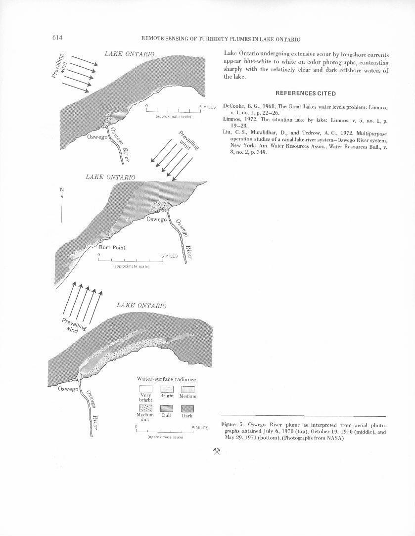
614 REMOTE SENSING OF TURBIDITY PLUMES IN LAKE ONTARIO
LAKE ONTARIO
Very Bright Medium bright
Lake Ontario undergoing extensive scour by longshore currents appear blue-white to white on color photographs, contrasting sharply with the relatively clear and dark offshore waters of the lake.
REFERENCES CITED
5 MILES DeCooke, B. G., 1968, The Great Lakes water levels problem: Limnos,v. l,no. l,p. 22-26.
Limnos, 1972, The situation lake by lake: Limnos, v. 5 no 1 p19-23.
Liu, C. S., Muralidhar, D., and Tedrow, A. C., 1972, Multipurpose operation studies of a canal-lake-river system-Oswego River system, New York: Am. Water Resources Assoc., Water Resources Bull v 8, no. 2, p. 349.
5 MILES
(approximate scale)
Figure 5. Oswego River plume as interpreted from aerial photo graphs obtained July 6, 1970 (top), October 19, 1970 (middle), and May 29, 1971 (bottom). (Photographs from NASA)

Jour. Research U.S. Geol. Survey Vol. 1, No. 6 , Sept.-Oct. 1973, p. 615-619
METHOD FOR ESTIMATING THE DIVERSION POTENTIALOF STREAMS IN EASTERN MASSACHUSETTS
AND SOUTHERN RHODE ISLAND
By GARY D. TASKER, Boston, Mass.
Prepared in cooperation with the Massachusetts Water Resources Commission
Abstract. A. simple method is proposed for estimating the probable magnitude and frequency of streamflow that is in excess of prede termined minimum streamflows required downstream in eastern Mas sachusetts and southern Rhode Island. Regional curves relate these annual volumes of streamflow excess to the average annual discharge and the median 7-day annual minimum flow of the site. Use of the curves is illustrated by a hypothetical example.
Predictions of large increases in demand for water in the near future have caused planners and designers to consider additional diversions of streamflow to meet future needs. It is not unusual in eastern Massachusetts and southern Rhode Island (fig. 1) to pump water in excess of a legislated minimum flow from the stream to an off-channel storage reservoir. Therefore, proper evaluation of streamflow-diversion potential requires knowledge of the probable magnitude and frequency of streamflow in excess of a predetermined minimum stream- flow.
Planners and designers desire a simple method that will give first approximations of the diversion potential of streams at sites where no continuous streamflow records are available. To help fulfill this desire, regional curves have been defined that relate annual volumes of streamflow excess to the average annual discharge and the median 7-day annual minimum flow.
DEVELOPMENT OF CURVES
Six gaging stations (table 1) were selected to represent the streams in the area. The stations were selected because each has at least 20 years of record, and the streams are not highly regulated. Diversion-probability curves for the six gaging stations are computed by the method proposed by Collings (1968). These curves assign a probability of occurrence to streamflow in excess of a specified discharge at a selected site and are computed by the following steps: 1. For each year during the period of record, the minimum
streamflow required to pass downstream (F) is sub tracted from the daily mean discharge, and the remaining discharge is summed to determine the
NEW HAMPSHIRE
ATLANTIC
OCEAN
50 MILES
Figure 1. Map of eastern Massachusetts and southern Rhode Island, showing the location of drainage basins (patterned) and gaging stations (table 1).
annual volume of streamflow in excess of F. These computations were greatly facilitated by use of a computer program developed by A. W. Burns, U.S. Geological Survey, Boston.
2. A cumulative frequency distribution of the annual volume of streamflow in excess of F is plotted for several values of F.
615

616 DIVERSION POTENTIAL OF STREAMS, MASSACHUSETTS AND RHODE ISLAND
Table 1. Measured discharge and median 7-day annual minimum flow at gaging stations
Station No.
1. .....
2.
3.
4.
5.
6.
Station name
Byfield, Mass.
near Ipswich, Mass.
. Charles River atCharles River Village, Mass.
, Adamsville Brook,at Adamsville, R.I.
near Norton, Mass.
. Pawcatuck Riverat Wood River Junction, R.I.
Dgage
21.6
124
184
7.91
42.4
100
Mean annual
ft 3 sec-'ami-2 )
1.58
1.59
1.59
1.76
1.67
1.84
Median annual 7-day
minimum flow (ft 3 sec- 'mi-2 )
0.029
.048
.142
.020
.113
.384
50
20
Q 10
biHty
0 20 40 60 80 100
MINIMUM FLOW ABOVE WHICH DIVERSION MAY OCCUR, IN CUBIC FEET PER SECOND
Figure 2. Diversion-probability curves for Wading River near Norton, Mass.
3. The streamflow in excess of F for a selected frequency is determined from the cumulative frequency distribu tion and plotted against the several values of F.
. Diversion-probability curves for Wading River near Norton, Mass., are shown in figure 2 as an example.
For each of the six stations, a straight line on semilog- arithmic paper provides a very good fit of the points computed by the above method. Therefore, the diversion-probability curves for these stations may be described by an equation of the form
(i)where
V is the annual potential diversion, in units of volume, F is the minimum streamflow above which diversion may occur, and 6 0 and 6 t are regression constants for a given stream site and probability (chance that a volume less than V will be available for diversion in any one year).
Although the constants 60 an(i ^i are estimated graphically in this study, they can be estimated by standard least-squares techniques by the following transformations:
log V - log b 0 + F log b i ,let V' = log F, 6 0 ' = log 6 0 , and 6 t ' = log 61 ,
then
(2)
which is the form of solution given by standard-regression computer programs for the independent variable F and dependent variable V'. Taking the inverse transforms, b 0 = lO^o7 and 61 = ID**'', enables the reconstruction of equation 1 or, equivalently, in terms of the coefficients from the standard program,
F = 10<V +*,'* ). (3)
This fit can be solved to get the set(6 0 >6i) f°r every combination of stream site and probability level.
Regression constant 6 0 equals the annual volume of stream- flow at a selected probability level. Therefore, it is expected that areal variations in 6 0 would be related to an index of areal variations in annual discharge (fig. 3). The average annual discharge was selected as an index of annual discharge because it can be estimated at ungaged sites in the area from runoff maps (Knox and Nordenson, 1955) or from regional formulas (Johnson, 1970).
0.8
0.7
0.6
0.5
0.2 I i i i I I i I1.5 1.6 1.7 1.8
AVERAGE ANNUAL DISCHARGE, (5, IN CUBIC FEET PER SECOND PER SQUARE MILE
Figure 3. Relation between b 0 and average annual discharge, Q. Data points for each probability level are gaging stations used in this report (fig. 1, table 1).

TASKER 617
Regression constant 6 t defines the slope of the semilog curve and depends largely on how streamflow is distributed throughout the year. Consider two streams, A and B, which have equal average annual discharge but whose average within-year distribution of streamflow is represented by the flow-duration curves shown in figure 4. When F = 0, the
100
50
20
I III
900 20 30 50 70 8(
TIME INDICATED DISCHARGE WAS EQUALED OR EXCEEDED, IN PERCENT
Figure 4. Flow-duration curves.
average annual potential diversions for both streams are equal to the average annual discharge. As F increases to F = Q it is apparent that the average annual potential diversion (area under the curve and above the line Q = F) for stream A will be greater than or equal to that of stream B for all values of F. Therefore, it would be expected that 6j could be related to an index of the within-year distribution of streamflow (fig. 5). In eastern Massachusetts and southern Rhode Island, as in eastern and southern Connecticut (Thomas, 1966), the within-year distribution of streamflow is greatly influenced by the hydrologic properties, of the unconsolidated deposits and the average flow is largely controlled by climatological factors. Because of the similarity of climatological factors and dif ferences in hydrologic properties of the unconsolidated de posits over the area, the areal variation in average flow is small compared to the areal variation in low-flow characteristics. Therefore, a single low-flow value can be an effective index of the within-year distribution of streamflow. The median 7-day annual minimum flow was selected as an index of the within-year distribution of streamflow because it can be estimated from base-flow measurements or, in southeastern Massachusetts, from maps of ground-water availability (Tasker, 1972).
0.6
0.3
0.2
T '
0.01 0.02 0.05 0.1 0.2 0.5
MEDIAN 7-DAY ANNUAL MINIMUM FLOW, IN CUBIC FEET PER SECOND PER SQUARE MILE
Figure 5. Relation between b t and the median 7-day annual minimum flow, Qm , 7 . Data points for each probability level are gaging stations (fig. 1, table 1).
In figure 3, coefficient 6 0 is related to average discharge by
60 = <*0 + 0o(? (4)
for each probability level. In figure 5, coefficient b t is related to the medium 7-day annual minimum flow (Qn\ 7)
61 = Iog@ mj (5)
for each probability level. These relations allow equation 1 to be expressed directly in terms of stream discharge characteris tics for a particular probability level, or
The parameters of this equation cannot be estimated directly by linear least squares, but can be estimated by the previously described procedure of estimating 6 0 and b\ for each basin and probability level and then relating these parameters to
.flow characteristics as in equations 4 and 5.This method ignores the possible cross correlation of 6 0 and
6j (correlation coefficient equal to 0.02), as well as other factors that might further refine the relations. However, there are the physical reasons described above for the relations shown in figures 3 and 5, and the relations are statistically significant at greater than the 90-percent level. Comparisons of the potential diversion observed from streamflow records with that estimated using figures 3 and 5 and equation 1 were made for values of F - 1.00 and 0.25 and for probabilities of 0.50, 0.20, and 0.10 (fig. 6). The estimated potential diversion

618 DIVERSION POTENTIAL OF STREAMS, MASSACHUSETTS AND RHODE ISLAND
100
ZQ~z zo
1 10 100
OBSERVED POTENTIAL DIVERSION, IN THOUSANDS OF CUBIC FEET PER SECOND-DAYS
Figure 6. Comparison of observed and estimated streamflow excess for long-term stations.
plotted within 10 percent of the observed value in 34 of the 36 points tested and within 5 percent in 24 of the 36 points. For the six long-term stations (table 1) it is found that the volume of streamflow in excess of 0.5 ft3 sec" 1 mi"2 for the 1967 water year has a probability range of 0.35 to 0.54, with an average probability of 0.49. Assuming the 1967 streamflow excess for any unregulated site in the area has a probability of occurrence of 0.49, the volume of streamflow in excess of 0.5 ft3 sec" 1 mi"2 estimated by the described method at the 0.49 probability level should approximate that observed in 1967 if the method is reliable. There are five short-term unregulated gaging stations in the area for which continuous records of discharge for the 1967 water year are available. Observed values of streamflow excess for the short-term stations for the 1967 water year are plotted against the values estimated by the described method in figure 7. The close agreement between the estimated and observed values in figures 6 and 7 indicates that fairly reliable estimates of potential diversion in terms of probability can be made with little effort.
Potential diversion is usually calculated from gaging station records during a critical period, usually the 1966 water year, and extrapolated to the site of interest. However, the proposed method will allow planners and designers to assign a proba bility to potential diversion and compare diversion of stream- flow with alternative methods of obtaining water, such as surface storage or ground-water wells.
LIMITATIONS
Applicability of empirical relations of this type to a site is dependent on similarity of the flow regimen at the site to that at the stations on which the relations are based. Consequently,
So 20,000
$LU< 10,000
5000
200°
ZujO
_i u u-iU. £E 0-
UJ 3 I-Q O < 2SoEFtfc/) ^JUJ </3
1000
EXPLANATION
7 Old Swamp River near South Weymouth, Mass.
8 Indian Head River at Hanover, Mass.
9 Dorchester Brook near Brockton, Mass.
10 Segreganset River near Dighton, Mass.
11 West Branch Palmer River near Rehoboth, Mass. /
/
Line of equality
1000 2000 10,000 20,000 50,000
OBSERVED STREAMFLOW IN EXCESS OF 0.5 CUBIC FEET PERSECOND PER SQUARE MILE DURING THE 1967 WATER YEAR,
IN CUBIC FEET PER SECOND-DAYS PER SQUARE MILE
Figure 7. Comparison of streamflow excess observed at short-term stations in 1967 and estimated streamflow excess at the 0.49 probability level.
the relations apply only to streams with virtually natural flow and whose drainage area, average annual discharge, and median 7-day minimum flow fall within the range of values given in table 1. In general, the relations would not apply to streams that are highly regulated, drain highly urbanized areas, or have a very large basin storage capacity.
In using figures 3 and 5 in connection with equation 1, F must be expressed in cubic feet per second per square mile and the estimate of V is given in thousands of cubic feet per second-days per square mile.
EXAMPLE
The following hypothetical example illustrates the use of the curves. A planner wants to know the median amount of diversion expected from a stream to supplement storage in a nearby reservoir. The unregulated stream has a drainage area of
10 mi2 , an average annual runoff of 1.70 ft3 sec' 1 mf2 , and a median 7-day annual minimum flow of 0.07 ft3 sec" 1 mi"2 . Requirements of downstream users will allow diversion of the flow exceeding 5 ft3 /sec. The proposed diversion system has a
maximum capacity of 5 ft3 /sec.Entering figure 3 with the average annual discharge for the
basin (1.70 ft3 sec' 1 mi'2 ), 6 0 for a probability of 0.50 (median) is determined as 0.62. Entering figure 5 with the median 7-day annual minimum flow for the basin (0.07 ft3 sec" 1 mi" 2 ), 61 for a probability of 0.50 is determined as 0.57. Substituting the values of F equal to 0.5 ft3 sec" 1 mi"2 , 6 0 equal to 0.62, and b\ equal to 0.57 into equation 1, the median annual volume of diversion in excess of 5 ft3 /sec is estimated as 4,680 ft3 sec" 1 days.

TASKER 619
At times, streamflow may exceed both the downstream requirement and the capacity of the diversion system. The median annual volume of water available from streamflow, after downstream requirements are met and beyond the capacity of the diversion system, may be determined from figures 3 and 5 and equation 1, as before, by considering F as the sum of the downstream requirements and the capacity of the diversion system (0.5 + 0.5). This volume is estimated as 3,530 ft3 sec' 1 days. The difference of 1,150 ft3 sec' 1 days between the two volumes (4,680 and 3,530 ft3 sec' 1 days) is the estimated median annual volume of water available for diversion from the stream to the reservoir.
Similarly, figures 3 and 5 and equation 1 can be used to estimate the annual volumes that have a 20- or 10-percent chance of not being exceeded in any one year.
REFERENCES CITED
Collings, M. R., 1968, Method of volume-diversion analysis of a stream,in Geological Survey Research 1968: U.S. Geol. Survey Prof. Paper600-C, p. C199-C203.
Johnson, C. G., 1970, A proposed streamflow-data program for centralNew England: U.S. Geol. Survey open-file rept., 49 p.
Knox, C. E., and Nordenson, T. J., 1955, Average annual runoff andprecipitation in the New England New York area: U.S. Geol.Survey Hydrol. Inv. Atlas HA-7.
Tasker, G. D., 1972, Estimating low-flow characteristics of streams insoutheastern Massachusetts from maps of ground-water availability,in Geological Survey Research 1972: U.S. Geol. Survey Prof. Paper800-D, p. D217-D220.
Thomas, M. P., 1966, Effect of glacial geology upon the timedistribution of streamflow in eastern and southern Connecticut, inGeological Survey Research 1966: U.S. Geol. Survey Prof. Paper550-B, p. B209-B212.


Jour. Research U.S. Geol. Survey Vol. l,No.5,Sept.-Oct. 1973, p. 621 625
CHANGES IN FLOODFLOW CHARACTERISTICS OF A RECTIFIED CHANNEL CAUSED BY VEGETATION, JACKSON, MISSISSIPPI
By K. V. WILSON, Jackson, Miss.
Work done in cooperation with the City of Jackson
Abstract. Extreme changes in velocity, stage, and Manning's rough ness coefficient, n, were observed during the first year after canalization of Hanging Moss Creek at Jackson, Miss. Additional changes were observed during the following 8 years. The channel, constructed during the summer of 1963, had a 50-foot-wide bottom, 2:1 side slopes, and 12-foot depth. In March 1964, average velocities of 7.8 feet per second were measured at a 5'/2-foot depth in the clean channel and Manning's n was computed to be 0.022. In October 1964 the average velocity was 3.2 fps at a 5'/2-foot depth and Manning's n was 0.045. The channel was then lined with fairly thick vegetation consisting of small willows, weeds, and grass. In October 1970 (summer foliage existing) the average velocity was 2.0 fps at a 5'/2-foot depth and Manning's n was 0.07. Willow trees, 8 to 10 feet high, then lined the channel. In March 1971 (barren foliage), Manning's n was 0.05. In March 1972 (barren foliage), Manning's n was increased to 0.07. These observations indicate that the commonly used values of Manning's n for channel rectification (0.02-0.03) are low and that the carrying capacity of earthen channels may be reduced 50 percent as a result of only 1 year's growth of vegetation and 70 percent as a result of 8 year's growth. The carrying capacity during summer foliage is approximately two-thirds the carrying capacity during barren winter foliage.
This paper evaluates changes with time, velocity, Manning's n, and flood profiles for the rectified channel of Hanging Moss Creek at Jackson, Miss. Wilson in 1968 (p. 57 59) described changes observed during the first 3 years after construction.
During the summer of 1963, the rectification of Hanging Moss Creek was extended 11,000 feet upstream from Ridge- wood Road by using the following design criteria: 1. 50-foot-wide-bottomed earthen channel with 2:1 side
slopes approximately 12 feet deep.Uniform grade of 0.0020 foot per foot for 2,500 feet
downstream from Interstate Route 55 (formerly U.S. Highway 51) and 0.0014 foot per foot for 3,500 feet upstream from Interstate Route 55.
Discharge of 5,900 cfs in the vicinity of Interstate Route55.
Roughness coefficient (Manning's n) of 0.045.
2.
3.
4.
FLOODFLOW CHARACTERISTICS AT INTERSTATE ROUTE 55
Flood data collected at the Interstate Route 55 gage show an extreme variation in the new channel's characteristics during the first year after canalization and continued change during the next 8 years.
The design flow line of the new channel at the downstream side of Interstate Route 55 was at an elevation (1929 datum) of 269.91 feet above sea level, which is the culvert flow-line elevation. The design stage-discharge, stage-velocity, and stage- area relation, with an assumed Manning's n of 0.045, is shown on figure 1. The same relations as measured March 1964, October 1964, February 1966, October 1970, March 1971, and March 1972 are also shown on figure 1. All measurements were made at the downstream service road of Interstate Route 55, where the cross-sectional area approximates the designed channel. A comparison of these relations at different times
reveals the following:1. By March 2, 1964, scouring and filling of half a foot in
the channel reduced the cross-sectional area between the elevations of 274 and 275 feet to about 10 percent less than the designed area. The third measurement of March 2, 1964, indicated an abrupt 10-percent increase in channel area and in discharge at the 275-foot stage. The average velocity at the 275-foot stage was 7.8 fps, or about double the design velocity. With this greatly increased velocity and slightly reduced area, the stage corresponding to the mean annual flood of 2,000 cfs was 274.5 feet, or 2.3 feet lower than the design stage of 276.8 feet.
2. By October 1964, moderately thick vegetation lined the new channel. The channel area, which now approximated the design area, showed no further increase in size. The average velocity at the 275-foot stage was reduced by the vegetation to only 3.2 feet per second, which is less than the design velocity at that stage. With extremely reduced velocity, the stage- discharge relation shifted about 2 feet. The stage correspond ing to the mean annual flood of 2,000 cfs was increased to 276.9 feet, which was within 0.1 foot of the design stage of 276.8 feet.
621

622 CHANGES IN FLOODFLOW OF RECTIFIED CHANNEL CAUSED BY VEGETATION
I ' I 1STAGE-DISCHARGE RELATIONS
Feb. 10, 1966
Mar. 2, 1964
EXPLANATION
March 1964 October 1970A A
October 1964 March 1971
February 1966 March 1972
I I I I I
STAGE-VELOCITYRELATIONS
1000 2000
DISCHARGE. IN CUBIC FEET PER SECOND
3000 0
AVERAGE VELOCITY, IN FEET PER SECOND
I I I I I I
STAGE-AREA RELATIONS
0 100 200 300 400 500 600
AREA, IN SQUARE FEET
Figure 1. Relation of stage to discharge, velocity, and area for an earthen canal constructed for Hanging Moss Creek at Jackson, Miss.
3. In February 1966 the data were similar to those for October 1964, but indicated that channel areas above the 276-foot stage were 20 percent larger than the design areas. It is probable that the consistency indicated by the 1964 and 1966 data results from summer foliage prevailing in October 1964 and winter barren foliage in February 1966.
4. By October 1970, thick vegetation lined the channel on both the bottom and banks. Channel areas were consistent with previous measurements. The average velocity at the 275-foot stage was reduced by vegetation to only 2.0 fps, which is about one-half the design velocity. With this extremely reduced velocity, the stage-discharge relation shifted an additional 1/2 feet. The stage corresponding to the mean annual flood of 2,000 cfs was increased to 278.4 feet, which is 1.6 feet higher than the design stage of 276.8 feet.
5. In March 1971 velocity increased to 3.4 fps which resulted in a 40 percent increase in discharge at a 276.5-foot stage. The velocity increase was due to the barren winter
foliage of the vegetation in the channel.6. In March 1972 the data were similar to those for
October 1970. Although foliage was minimal, the vegetation growth between March 1971 and March 1972 is accredited with reducing the channel's carrying capacity by 25 percent. In March 1972, the stage corresponding to the mean annual flood of 2,000 cfs was 278.4 feet, which is 1.6 feet higher than the design stage of 276.8 feet. The carrying capacity at the 278-foot elevation is 900 cfs less than the design capacity; therefore, it may be assumed that the Hanging Moss Creek channel, designed to carry a 50-year discharge of 5,900 cfs at a 12-foot depth will now carry no more than 5,000 cfs, which is less than a 25-year flood.
COMPUTATIONS OF MANNING'S n
The equation presented by Manning (1890, p. 161 207), one of the most commonly used open-channel flow formulas,
is 0 = " AR 3 S . where 0 is the discharge in cubic feet Y n > v 6
per second, n is the roughness coefficient, A is the cross-sec tional area of the channel in square feet, R is the hydraulic radius in feet, and 5 is the energy gradient. All these factors are physical measurements with the exception of the rough ness coefficient, which can be computed when other factors are known.
Values of Manning's n commonly used for designing earthen channels vary from 0.02 to 0.03. The calculated carrying capacity of a geometrically stable channel for any given slope is inversely related to this factor; therefore, if the n value is doubled as a result of changing channel conditions the carrying
capacity is reduced 50 percent.
Manning's n was computed for reaches upstream and downstream from Interstate Route 55 for seven floods (table 1). The n values shown in the table were obtained by using known discharges, the design cross section, and slopes between bridges 1,200 feet downstream and 2,750 feet upstream.
After the flood of March 2, 1972, a four-section reach beginning 450 feet upstream from Interstate Route 55 and extending 700 feet upstream was surveyed in detail. For this short reach the Manning's n was 0.073 as compared to 0.074 for the longer reach (see table 1). A photograph showing typical roughness of March 10, 1972, (n = 0.073) is shown on
figure 2.

WILSON 623
Table 1. Manning's n values, Hanging Moss Creek at Interstate Route 55 in Jackson, Miss., 1964 72
[Values for areas and wetted perimeters are from design cross section. Design flow line is 269.91 feet]
Date
Mar. 3, 1964 . . .
Oct. 4, 1964 Feb. 10, 1966 . . Oct. 13, 1970 . . Mar. 25, 1971 . . Mar. 2, 1972 ...
Stage (ft)
. 275.08 275.01
. 274.53
. 277.78
. 277.36
. 276.62
. 278.11
Discharge (cfs)
2,540 2,240
952 2,440 1,440 1,550 1,810
Area (sq ft)
312 306272 520 488 428 550
Wetted perimeter
(ft)
73.0 72.6 70.8 85.0 83.0 80.0 97.6
Slope (ft/ft)Upstream
1 0.0017 '.0017 '.0017 .00178 .00174 .00180 .00214
Downstream
2 0.0020 2 .0020 2 .0020 .00219 .00136 .00136 .00140
Computed nUpstream
0.020 .022 .043 .045 .068 .053 .074
Downstream
0.021 .024 .047 .049 .060 .046 .060
1 Estimated from profile of July 8, 1963 (slope was 0.00164).2 Design slope; assumed to exist during 1964.
Figure 2. Vegetation in channel 450 feet upstream from Interstate Route 55, March 10,1972 (n = 0.073).
During the floods of October 1964 and October 1970, summer foliage reduced the carrying capacity (increased re). In October 1970, re values were 20 to 25 percent greater than those for the following March and were approximately equal to those of March 1972. Changes in Manning's re, for the period 1964 72, in the reach upstream from Interstate Route 55 are shown on figure 3. These data indicate that n during summer foliage is one-third larger than n during barren winter conditions.
Photographs of the channel viewed upstream from Interstate Route 55 on March 25, 1971, March 29, 1971, September 9, 1971, and March 10, 1972, are shown in figure 4.
FLOOD PROFILES AND FLOW-LINE PROFILES
Floods on Hanging Moss Creek on February 10 and May 21, 1966, had peak discharges of 2,500 and 2,400 cfs, respec tively, at the gage at Interstate Route 55. These peak discharges may be expected to be exceeded on the average of once in about 3 years. Profiles of these floods are compared with the design profile of the 50-year flood on figure 5.
Moderately thick vegetation consisting of willows, weeds, and grasses lined the channel. Effect of the vegetation on the flood profiles is shown by an increase in stage downstream from Ridgewood Road. The design depth for 2,500 cfs at that point is about 10 feet. The vegetation caused the depth on February 10 and May 21, 1966, to be increased to about 11 feet. This is the difference in the water surface elevation of 272 feet and the flow line of 261 feet (fig. 5).
The flood of October 13, 1970, had a peak discharge of 1,700 cfs at the gage at Interstate Route 55. This flood may be expected to be exceeded on the average of once in about 2 years. A profile of this flood is shown on figure 5.
On October 13, 1970, willows and weeds, 8 to 10 feet high, and heavy summer foliage lined the channel. Effect of this vegetation on the flood profile was to raise it to or above the profile of February 10, 1966, at which time the discharge was 2,500 cfs at Interstate Route 55. Effect of vegetation was
1964 1965 1966 1967 1968 1969 1970 1971 19720.02
Figure 3. Changes in Manning's n, 1964 72, and dates of photographs in figure 4.

624 CHANGES IN FLOODFLOW OF RECTIFIED CHANNEL CAUSED BY VEGETATION
c DFigure 4. The channel viewed upstream from Interstate Route 55.
A. March 25, 1971 (near crest). Discharge, 1,600 cfs; stage at downstream service road, 276.8 feet.B. March 29, 1971. Rod (left center) at crest of March 25.C. September 9,1971. Summer foliage.D. March 10, 1972. Barren foliage; rod (upper left) at crest of March 2, 1972.
greatest at the downstream side of Ridgewood Road. The design depth for 1,700 cfs at that point is about 8/2 feet. The vegetation caused the depth on October 13, 1970, to be about 13 feet. The flood stages of October 13, 1970, equaled or exceeded those of February 10, 1966, throughout the 2-mile channel reach between Sylvia Street extension and Ridgewood Road, with the exception of a short reach, just upstream from
the Illinois Central Railroad, which had recently been cleared of vegetation.
The designed flow-line profile of Hanging Moss Creek between stations 10+00 and 133+00 is shown on figure 5. Cross sections were obtained upstream and downstream from all street, highway, and railroad crossings during the winter of 1968 by the U.S. Soil Conservation Service. Comparison o f
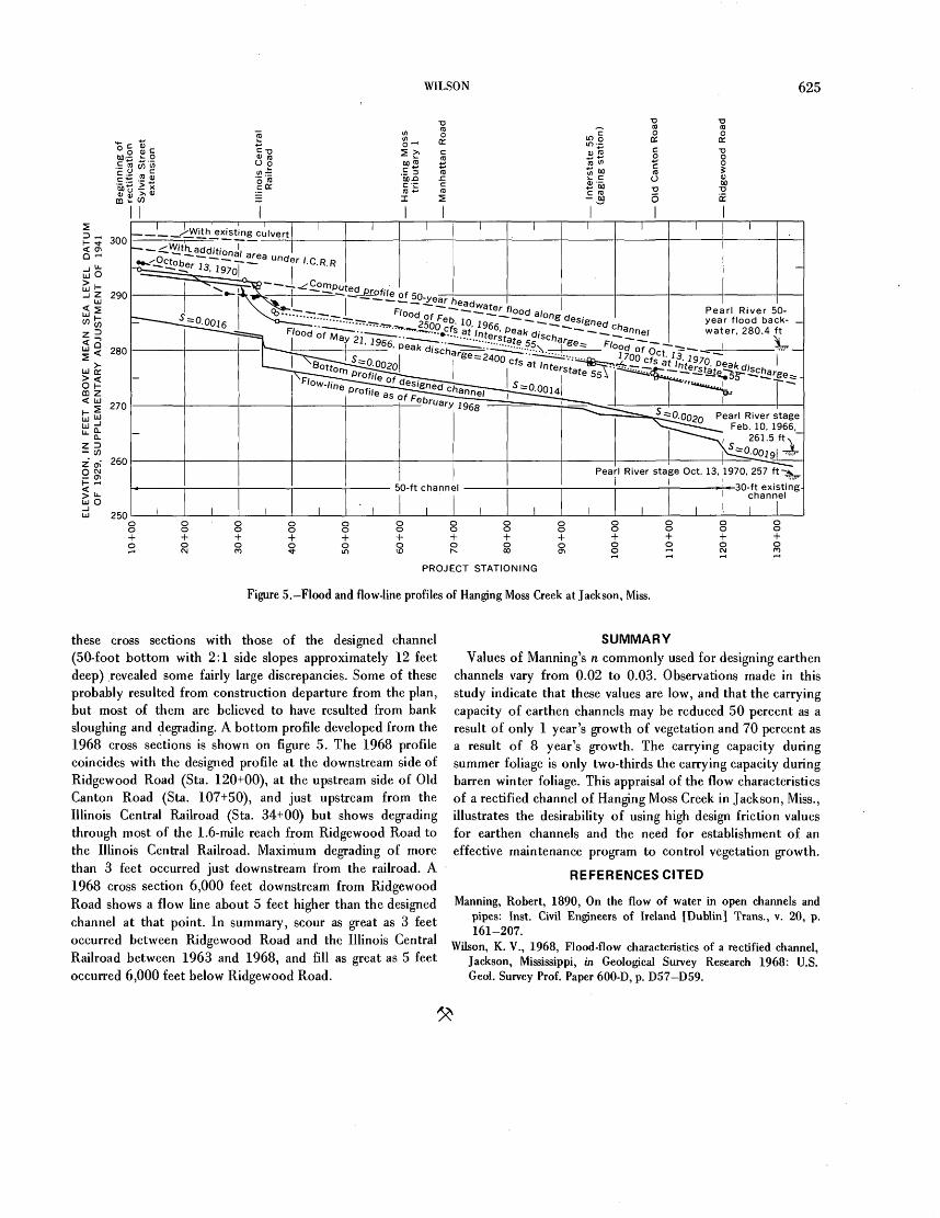
WILSON 625
I I ' I_ _x^With_existing culvert
Pearl River 50- year flood back- _ water, 280.4 ft
Pearl River stage Feb. 10, 1966,
261.5 ft "
Pearl River stage Oct. 13, 1970, 257
PROJECT STATIONING
Figure 5.-Flood and flow-line profiles of Hanging Moss Creek at Jackson, Miss.
these cross sections with those of the designed channel (50-foot bottom with 2:1 side slopes approximately 12 feet deep) revealed some fairly large discrepancies. Some of these probably resulted from construction departure from the plan, but most of them are believed to have resulted from bank sloughing and degrading. A bottom profile developed from the 1968 cross sections is shown on figure 5. The 1968 profile coincides with the designed profile at the downstream side of Ridgewood Road (Sta. 120+00), at the upstream side of Old Canton Road (Sta. 107+50), and just upstream from the Illinois Central Railroad (Sta. 34+00) but shows degrading through most of the 1.6-mile reach from Ridgewood Road to the Illinois Central Railroad. Maximum degrading of more than 3 feet occurred just downstream from the railroad. A 1968 cross section 6,000 feet downstream from Ridgewood Road shows a flow line about 5 feet higher than the designed channel at that point. In summary, scour as great as 3 feet occurred between Ridgewood Road and the Illinois Central Railroad between 1963 and 1968, and fill as great as 5 feet occurred 6,000 feet below Ridgewood Road.
SUMMARYValues of Manning's n commonly used for designing earthen
channels vary from 0.02 to 0.03. Observations made in this study indicate that these values are low, and that the carrying capacity of earthen channels may be reduced 50 percent as a result of only 1 year's growth of vegetation and 70 percent as a result of 8 year's growth. The carrying capacity during summer foliage is only two-thirds the carrying capacity during barren winter foliage. This appraisal of the flow characteristics of a rectified channel of Hanging Moss Creek in Jackson, Miss., illustrates the desirability of using high design friction values for earthen channels and the need for establishment of an effective maintenance program to control vegetation growth.
REFERENCES CITED
Manning, Robert, 1890, On the flow of water in open channels and pipes: Inst. Civil Engineers of Ireland [Dublin] Trans., v. 20, p. 161-207.
Wilson, K. V., 1968, Flood-flow characteristics of a rectified channel, Jackson, Mississippi, in Geological Survey Research 1968: U.S. Geol. Survey Prof. Paper 600-D, p. D57-D59.


RECENT PUBLICATIONS OF THE U.S. GEOLOGICAL SURVEY
(Books may be ordered from the Superintendent of Documents, Government Printing Office, Washington, D.C., 20402, to whom remittances should be sent by check or money order. Give title, series No., stock No. (shown in parentheses in this list), and catalog No. [shown in brackets])
Professional Papers
306-E. Geology and paleontology of Canal Zone and adjoining parts of Panama: Description of Tertiary mollusks (additions to gastropods, scaphopods, pelecypods: Nuculidae .to Malleidae), by W. P. Woodring. 1973. p. 453-539; 16 plates showing fossils. $1.75. (2401-00217) [119:16:306-E]
433-M. Relations among radionuclide content and physical, chemical, and mineral characteristics of Columbia River sediments, by J. L. Glenn, with a section on Sand and gravel mineralogy, by R. 0. Van Atta. 1973. p. M1-M52. 85</. (2401-00297) [19:16:433-M]
433-N. Radionuclides in transport in the Columbia River from Pasco to Vancouver, Wash., by W. L. Haushild, H. H. Stevens, Jr., J. L. Nelson, and G. R. Dempster, Jr. 1973. p. N1-N43. 754. (2401-00298) [119:16:433-N]
569-C. Hydrologic significance of lithofacies of the Cane River Formation or equivalents of Arkansas, Louisiana, Mississippi, and Texas, by J. N. Payne. 1972 (1973). p. C1-C17; plates in separate case. $10.90(2401-00246) [119:16:569-C]
599-H. Geology of the Sierra Madera cryptoexplosion structure, Pecos County, Tex., by H. G. Wilshire, T. W. Offield, K. A. Howard, and David Cummings. 1972 (1973). p. H1-H42; plates in pocket. $2. (2401-00238) [119:16:599-H]
629-B. Igneous rocks in the Bingham mining district, Utah, by W. J. Moore. 1973. p. B1-B42. 85tf. (2401-00274) [119:16:629-8]
697. Landslides of Rio de Janeiro and the Serra das Araras escarp ment, Brazil, by F. 0. Jones. 1973. 42 p.; plates in pocket. $1.50. (2401-2126) [119:16:697]
717. Geology and ground-water characteristics of the Hanford Reser vation of the U.S. Atomic Energy Commission, Wash., by R. C. Newcomb, J. R. Strand, and F. J. Frank. 1972 (1973). 78 p.; plates in pocket. $2.60. (2401-00241) [119:16:717]
729-A. Geology of pre-Tertiary rocks in the northern part of Yellowstone National Park, Wyo., by E. T. Ruppel, with a section on Tertiary laccoliths, sills, and stocks in and near the Gallatin Range, Yellowstone National Park. 1972 (1973). p. A1-A66; plates in pocket. $2.60. (2401-00242) [119:16:729-A]
732-B. Scour and fill in Tujunga Wash A fanhead valley in urban southern California-1969, by K. M. Scott. 1973. p. B1-B29. 704. (2401-00322) [119:16:732-8]
734-A. Harebell Formation (Upper Cretaceous) and Pinyon Conglom erate (uppermost Cretaceous and Paleocene), northwestern Wyoming, by J. D. Love. 1973. p. A1-A54. $1. (2401-00316) [119:16:734-A]
736. Regional geophysical investigations in the central Colorado Plateau, by J. E. Case and H. R. Joesting. 1972 (1973). 31 p.; text and plates in case. $5.60. (2401-00222) [I 19:16:736]
757. Sedimentary framework of the western Gulf of Maine and the southeastern Massachusetts offshore area, by R. N. Oldale, Elazar Uchupi, and K. E. Prada. 1973. 10 p.; plates in pocket. $1.75. (2401-00304) [119:16:757]
758-A. Geology and mineral deposits of the Chulitna-Yentna mineral belt, Alaska, by C. C. Hawley and A. L. dark. 1973. p. Al-AlO; plates in pocket. $1.25. (2401-00335) [119:l6:758-A]
764. Stratigraphy of the southern Coast Ranges near the San Andreas fault from Cholame to Maricopa, Calif., by T. W. Dibblee, Jr. 1973. 45 p. 80^. (2401-00300) [119:16:764]
766. Foraminifera of the North Pacific Ocean, by P. B. Smith. 1973.27 p.; 4 plates showing fossils. 854. (2401-00295) [I 19:16:766]
775. Petrography of some granitic bodies in the northern White Mountains, Calif.-Nev., by D. F. Crowder and D. C. Ross. 1973.28 p. 704. (2401-00332) [119:16:775]
797. Petrology of the welded tuff of Devine Canyon, southeastern Oregon, by R. C. Greene. 1973. 26 p. 654. (2401-00331) [119:16:797]
801. Jurassic paleobiogeography of Alaska, by R. W. Imlay and R. L. Detterman. 1973. 34 p. 654. (2401-00347) [119:16:801]
807. Geochemical anomalies of a clay pit area, Callaway County, Mo., and related metabolic imbalance in beef cattle, by R. J. Ebens, J. A. Erdman, G. L. Feder, A. A. Case, and L. A. Selby. 1973. 24 p. 654. (2401-00337) [119:16:807]
820. United States mineral resources, D. A. Brobst and W. P. Pratt, Editors. 1973. 722 p. $9.15. (2401-00307) [I 19:16:820]
838. Geologic and seismologic aspects of the Managua, Nicaragua, earthquakes of December 23,1972, by R. D. Brown, Jr., P. L. Ward, and George Plafker. 1973. 34 p.; plate in pocket. $1.25. (2401-00340) [119:16:838]
Bulletins
1332-D.' Lithologic characteristics of Pliocene rocks cored at Elk Hills, Kern County, Calif., by W. M. Berryman. 1973. p. D1-D56; plate in pocket. $1.20. (2401-00317) [119:3:1332-0]
1365. Geochemical reconnaissance of the Santa Rita Mountains, southeast of Tucson, Ariz., by Harold Drewes. 1973. 67 p.; plates in pocket. $1.25. (2101-00281) [119:3:1365]
1366. Bibliography of the geology and mineralogy of the rare earths and scandium to 1971, by J. W. Adams and E. R. Iberall. 1973. 195 p. $2.10. (2401-2154) [119:3:1366]
1367. A disseminated silver-lead-zinc sulfide occurrence at Hahns Peak, Routt County, Colo., by E. J. Young and Kenneth Segerstrom. 1973. 33 p.; plates in pocket. $1.50. (2401-00276) [119:3:1367]
1375. Lithologic characteristics of upper Oligocene and Miocene rocks drilled at Elk Hills, Kern County, Calif., by W. L. Adkison. 1973. 113 p.; plates in pocket. $1.50. (2401-00339) [119:3:1375]
1376. Some results of geochemical sampling in McCormick County, S.C., by Henry Bell HI. 1973. 22 p.; plates in pocket. $1.75. (2401-00334) [No. 119:3:1376]
1381. Geochemical characteristics of mineralized breccia pipes in the Red Mountain district, San Juan Mountains, Colo., by F. S. Fisher and W. P. Leedy. 1973. 43 p. 4,54. (2401-00320) [119:3:1381]
1382-A. Chemical composition of naturally occurring fluids in rela tion to mercury deposits in part of north-central California, by Ivan Bames, M. E. Hinkle, J. B. Rapp, Chris Heropoulos, and W. W. Vaughn. 1973. p. A1-A19. 4,54. (2401-00296) [119:3:1382-A]
1382-B. Radioelement and trace-element content of the lone Forma tion, central California, by H. A. Wollenberg and F. C. W. Dodge. 1973. p. B1-B17. 30^. (2401-00328) [119:3:1382-8]
Water-Supply Papers
1817-D. Preparative free-flow electrophoresis as a method of frac- tionation of natural organic materials, by J. A. Leenheer and R. L. Malcolm. 1973. p. D1-D14. 35tf. (2401-00293) [119:13:1817-D]
1865. Water resources and geology of Mount Rushmore National Memorial, S. Dak., by J. E. Powell, J. J. Norton, and D. G. Adolphson. 1973. 50 p.; plate in pocket. $1.25. (2401-00323) [119:13:1865]
2029-B. Generalization of stream-temperature data in Washington, by M. R. Collings. 1973. p. B1-B45. 30</. (2401-00302) [119:13:2029-8]

U.S. GOVERNMENT PRINTING OFFICEPUBLIC DOCUMENTS DEPARTMENT
WASHINGTON, D.C. 20402
OFFICIAL BUSINESS
PtNALTY FOR PRIVATE USE $300
POSTAGE AND FEES PAID
U.S. GOVERNMENT
PRINTING OFFICE 375