Geological Structures: a Practical Introduction

© John W.F. Waldron and Morgan Snyder

2020

University of Alberta

Geological Structures: a Practical Introduction by John Waldron and Morgan Snyder is licensed under a Creative Commons Attribution-NonCommercial 4.0 International License, except where otherwise noted.

Contents

Acknowledgements vii

About this document ix

A. Geological Structures 1

B. Orientation of Structures 5

• Lab 1. Orientation of Lines and Planes 19

C. Primary Structures 23

• Lab 2. Cross-sections and Three-point Problems 39

D. Stereographic Projection 45

• Lab 3. Working with Stereographic Projections 51

E. Folds 63

• Lab 4. Introduction to Folds 79

• Lab 5. More about Folds 81

F. Boudinage 85

G. Kinematic Analysis and Strain 87

H. Fabrics 95

• Lab 6. Fabrics and Folds 105

I. Dynamic Analysis: Stress 107

J. Fractures 113

• Lab 7. Fractures 121

K. Faults 129

Lab 8. Measuring Fault Slip 143

L. Tectonic Environments of Faulting 147

• Lab 9. Field Mapping 157

• Lab 10. Fold and Thrust Belts 161

M. Shear Zones 167

N. Extraterrestrial Impact Structures 175

Glossary of terms 181

Acknowledgements

This manual incorporates exercises and contributions from previous instructors of the course EAS 233 Geologic

Structures at the University of Alberta, including Henry Charlesworth, Larry Heaman, Fred Clark, Shawna White, and

others. It has also benefited from the proof-reading assistance of Marilyn Huff and from input from several generations

of teaching assistants. These contributions are gratefully acknowledged.

The Open Educational Resource version of this manual benefitted from an Open Educational Resources grant from the

University of Alberta, and the helpful advice and assistance of Krysta McNutt, Michelle Brailey and Jemma Forgie.

Acknowledgements | vii

About this document

Learning Outcomes

By the end of this course on Geological Structures you should be able to:

• Describe common geological structures in maps, outcrops and samples, using terms that can be

understood by other geologists;

• Construct geological cross-sections based on evidence in maps;

• Calculate angles and distances between geological structures using data from geological maps;

• Interpret the history of changes in the Earth’s crust that produced geological structures observed at the

Earth’s surface.

Preliminaries

This manual is about structures that occur within the Earth’s crust. Structures are the features that allow geologists

to figure out how parts of the Earth have changed position, orientation, size and shape over time. This work requires

careful observation and measurements of features at the surface of the Earth, and deductions about what’s below the

surface. The practical skills you will learn in this course form the foundation for much of what is known about the history

of the Earth, and are important tools for exploring the subsurface. They are essential for Earth scientists of all kinds.

The course that this document supports is about doing structural geology. It’s not possible to be a good geologist (or to

pass the course) just by learning facts. You have to be able to solve problems. Do your lab work conscientiously and get

as much as possible done during lab sessions when instructors are available to help you.

This manual consists of both readings and lab exercises, which alternate through the text. The readings are designed

to be read and understood outside the lab sessions, whereas the labs contain specific instructions and questions to be

completed. Before each lab, be sure you have covered the readings that come immediately before it.

Many problems in structural geology involve thinking in three dimensions. This is the largest challenge that you will face

in working with the material in this book. Different people use different strategies for thinking in 3D. Your instructors

will sometimes be able to offer a range of strategies and techniques. Make use of their skills whenever you have

difficulty.

This manual was written to support the course “EAS233 Geologic Structures” at the University of Alberta in Canada. The

course is typically taught between January and April. During January and February it is too cold for effective geological

fieldwork, so the outdoor lab (lab 9) takes place toward the end of the class. In a warmer climate, the data collection

part of this lab could be done earlier in the course.

About This Course | ix

A word on language: Canadian English, and Canadian geology, follow a mixture of British and American traditions. For

example, British geologists will always speak of “geological structures” whereas Americans may say “geologic structures”.

The British Carboniferous Period is equivalent to the Mississippian and Pennsylvanian in the U.S. Canadian geology

follows a mixture of both traditions which can sometimes seem aggravatingly inconsistent. However, we encourage

readers to embrace this diversity in the interests of encouraging communication between those interested in the Earth

on both sides of the Atlantic!

Things you should know before you start

You should have completed a course in introductory geology. Here are some of the things you are expected to know.

• Maps and map scales: You should be able to convert a map scale expressed as a representative fraction (e.g.

1:50,000) to a map scale expressed in metric or imperial length units (2 cm = 1 km) and draw a scale bar based on

either. You should understand topographic contours and should be able to look at a map with topographic contours and identify hills, valleys, and predict which way streams are flowing.

• Plate tectonics: Know the difference between continental and oceanic lithosphere, and the three major types of

plate boundary: spreading centres, subduction zones, transform faults.

• Minerals: Common rock-forming minerals such as quartz, feldspar, mica, amphibole, calcite.

• Basic rock types: You should know the names of basic rock types and be able to identify them. At minimum, these

should include the following:

• Igneous rocks: granite, diorite gabbro, peridotite, rhyolite, andesite, basalt, tuff.

• Sedimentary rocks: conglomerate, sandstone, mudstone and shale, limestone, dolostone, coal, chert, rock

salt, gypsum.

• Metamorphic rocks: slate, schist, gneiss, granofels, quartzite, marble.

• Geological time: You should know the sequence of eons: Archean, Proterozoic, Phanerozoic, and within the

Phanerozoic you should know the names of the eras and periods by heart.

• Paleozoic: Cambrian, Ordovician, Silurian, Devonian, Carboniferous (Mississippian, Pennsylvanian), Permian.

• Mesozoic: Triassic, Jurassic, Cretaceous.

• Cenozoic: Paleogene, Neogene, Quaternary.

We will assume you are familiar with these terms and their meanings. If any of them are unfamiliar, now is the

time to review the material from your introductory classes and make sure you know them!

Before you work on the first assignment

Before you come to lab, read the relevant sections of this book, and any other assigned reading, carefully.

• Set up your work on each assignment with a cover page so that it’s easy to review and mark. The first page of each

set of answers for the assignments should consist of a sheet of paper with (1) your name, (2) EAS 233, (3)

Assignment X, (4) your laboratory section, and (5) the date of submission.

• Pass in only those pages of this book on which you have done work. Keep the instructional pages when possible, so

x | About This Course

that you can refer to them while your assignment is being marked.

• Along with the answer to each problem for an assignment, you should show the work that enabled you to arrive at

the answer. There are several reasons for this. First, it’s sound scientific practice. Second, you are less likely to

make mistakes. Third, if your work shows that you used a correct method but made a minor error, you may still get

most of the marks; a wrong answer on its own is not worth any marks at all!.

• Make use of your lab sections and TAs. Try to solve and complete an assignment during your lab section and hand

your assignment in at the end of your lab section. If you need more time to complete an assignment, there will be

deadlines for handing them in; these will be announced by the TAs in the first lab.

• If you make a mistake that can’t be corrected with a simple erasure, it’s ok to place a piece of tracing paper over

the original version and complete your answer on the tracing paper. Note that you don’t need to trace the entire

question. Just mark the corners or some other conspicuous points so that someone marking your work can place

your tracing paper over a clean original to see what you have done.

• Some questions are designated for self-marking. These will be marked with an *asterisk. These will be assessed

only as ‘complete’ or ‘incomplete’ during marking, but they must be completed to obtain full marks for the lab.

Answers will be provided for checking during the following lab. You are advised to complete them conscientiously,

as the skills involved will be tested in the exams. If you find you have done poorly in a self-marked question, make

sure you know where you went wrong, or ask for help from a teaching assistant. Note that the rules for academic

integrity and plagiarism apply to the self-marking questions: an answer copied from someone else is a breach of the academic code of conduct and is subject to the same penalties as any other kind of copying.

• Completed labs should be placed in the appropriate slot for your lab section.

• Grading key if deadline is missed: Max. 70% after deadline; 0 (zero) after assignments were returned (typically your

next lab session).

Academic Integrity

All work you present for evaluation in any course must be your own work. It is an academic offense if you:

• present someone else’s work as your own (plagiarism);

• gain an unfair advantage in a test or an exam (cheating);

• distort the truth for advantage (misrepresentation of facts);

• encourage or help anyone else to do any of these things.

In this course you will sometimes benefit from discussions with other students as well as teaching assistants, especially

in the labs. Although this discussion may help you decide how to solve problems in structural geology, the actual answers you write down must be written in words and sentences composed by you alone, diagrams must be drawn by you, and any measurements or calculations must be carried out separately by you. It is not acceptable to share a calculator

in determining the answers to questions. Note that these rules apply to ‘self marking’ questions just as much as to

questions that will be given a numerical mark.

About This Course | xi

A. Geological Structures

Structural geology

What are geological structures?

If the Earth’s crust were completely uniform and homogeneous (the same everywhere), we would have great difficulty

figuring out anything about its history. Fortunately, the Earth’s crust contains structures of many kinds. Structures are

variations in the properties of the Earth’s crust. Those variations may be:

• Spatial variations: the rocks of the Earth’s crust vary from place to place, either on the surface or below; or

• Directional variations: rocks look different when viewed from different directions.

For example, where one type of rock contacts another, there is a geological boundary, a type of structure. Geological

boundaries include:

• faults

• bedding planes

• the edges of igneous intrusions (intrusive contacts)

• ancient erosion surfaces (unconformities)

You should have heard about all these types of boundary in your introductory courses. All these boundaries tell you

something about the geological history of the area where they are found.

Figure 1. Mapping a geological boundary

Even without looking at boundaries, you may be able to see structure in a rock unit: the properties of many rocks vary

with direction because the mineral grains are aligned with one another: we say the rock has fabric, another type of

structure.

A. Geologic Structures | 1

Figure 2. Microscopic thin section of a rock with fabric ( field of view 5 mm). The small dark minerals with a strong alignment are biotite mica. Larger grey minerals are mostly the aluminum-rich minerals staurolite and garnet. Light minerals are quartz and feldspar.

Such structures can tell us a great deal about the history of the Earth, and are critical for those seeking resources such

as water, petroleum, and minerals.

Some geological structures formed at the same time as the rocks in which they are found. These are primary structures.

Examples of primary structures include beds and laminae in sedimentary rocks like sandstone, or shale, and lava pillows

in extrusive igneous rocks like basalt. In general, you will learn most about primary structures in courses that deal

with the formation of various rock-types, but this introduction will cover some of the more important types of primary

structure, especially those that are important in figuring out Earth history.

Many structures are formed long after the rocks in which they are found. These are secondary structures. Secondary structures include folds, fractures, foliations in metamorphic rocks, and a host of other features. Most secondary

structures are products of deformation – the movement of parts of the crust relative to one another. Structural geology is mainly concerned with secondary structures, and therefore is mostly about the deformation of the Earth.

Tectonics is a closely related term to structural geology. Originally, tectonics referred to the mathematical and

geometrical description of geological structures at quite small scales. However, in the 1960’s it was found that large-

scale movements of the outer part of the Earth (the lithosphere) could be described by quite simple mathematical and

geometrical methods, and plate tectonics was born. Since then, the term tectonics has mainly referred to the study of

large-scale movements of the lithosphere and the structures that these have produced.

Structural analysis

The Earth’s crust contains structures almost everywhere, and the aims of structural geology are to document and

understand these structures. In general, work in structural geology is targeted at three different aims, or levels of

understanding.

2 | A. Geologic Structures

• Descriptive or Geometric analysis – what are the positions, orientations, sizes and shapes of structures that exist

in the Earth’s crust at the present day?

• Kinematic analysis – what changes in position, orientation, size, and shape occurred between the formation of the

rocks and their present-day configuration? Together, these changes are called deformation. Changes in size and

shape are called strain; strain analysis is a special part of kinematic analysis.

• Dynamic analysis – what forces operated and how much energy was required to deform the rocks into their

present configuration? Most often in dynamic analysis we are interested in how concentrated the forces were.

Stress, or force per unit area, is a common measure of force concentration used in dynamic analysis.

It is important to keep these three distinct. In particular, make sure you can describe structures first, before attempting

to figure out what moved where, and avoid jumping to conclusions about force or stress without first understanding

both the geometry and the kinematics of the situation.

Much of this book will focus on the descriptive or geometric objective, which is a foundation for further understanding.

Once you have thoroughly described structures, you will be able to proceed to kinematic and sometimes dynamic

conclusions.

Scale

Structural geologists look at structures at a variety of scales, ranging from features that affect only a few atoms

within mineral grains, to structures that cross whole continents. It’s convenient to recognize three different scales of

observation.

• Microscopic structures are those that require optical assistance to make them visible.

• Mesoscopic, or outcrop-scale structures are visible in one view at the Earth’s surface without

optical assistance.

• Macroscopic, or map-scale structures are too big to see in one view. They must be mapped to make them visible,

or imaged from an aircraft or a satellite.

Geological maps

One powerful representation of the geometry of rock structures is a geological, or geologic map. Geological maps

are created through the process of mapping in which outcrops are visited in the course of fieldwork, described, and

recorded on a topographic base map. The result is an outcrop map in which the observed rock types and structures

are recorded. In most areas, there will be gaps between the observed outcrops, where the bedrock is obscured by soil,

vegetation, or other types of overburden.

To make a geological map, some interpretation is necessary, in order to fill in the areas between the outcrops. In

most cases, some understanding of geological processes is required in order to come up with an interpretation. Figure

3a shows an outcrop map, and Fig. 3b shows an attempt at a geological map made without much understanding of

geological processes. Although it satisfies the observations in a simplistic way, it is unlikely to be correct. Figure 3c is a

more likely interpretation, made with some understanding of geological processes. Note that this, second version leads

to some kinematic interpretations. We can infer that perhaps parallel units B, C and D represent sedimentary layers, and

unit A is perhaps a younger intrusion because it cross-cuts them.

A. Geologic Structures | 3

Figure 3. (a) An outcrop map with (b) an unlikely interpretation and (c) a more likely interpretation, producing a reasonable geological map.

4 | A. Geologic Structures

B. Orientation of Structures

Lines and Planes

Linear and planar features in geology

Almost all work on geologic structures is concerned in one way or another with lines and planes.

The following are examples of linear features that one might observe in rocks, together with some kinematic deductions

from them:

• glacial striae (which reveal the direction of ice movement);

• the fabric or lineation produced by alignment of amphiboles seen in metamorphic rocks (which reveal the

direction of stretching acquired during deformation);

• and the alignment of elongate clasts or fossil shells in sedimentary rocks (which reveals current direction).

Examples of planar features include:

• tabular igneous intrusive bodies such as dykes and sills;

• bedding planes in sedimentary rocks;

• the fabric or foliation produced by alignment of sheet silicate minerals such as mica in metamorphic rocks, which

reveals the direction of flattening during deformation;

• joints and faults produced by the failure of rocks in response to stress (and which therefore reveal the orientation

of stress at some time in the past).

Notice that although several of the above descriptive observations lead to kinematic inferences, only the last one allows

us to make dynamic conclusions!

Bearings

To describe almost any structure, we need to say something about its orientation (also known as its attitude): Does it

run north-south, or perhaps east-west, or somewhere in between? A direction relative to north is called a bearing. In

most geologic work, bearings are specified as azimuths.

An azimuth is a bearing measured clockwise from north.

An azimuth of 000° represents north, 087° is just a shade north of east, 225° represents southwest, and 315° represents

NW.

B. Orientation of Structures | 5

Figure 1: Compass used to measure an azimuth – in this case the strike of a bedding plane.

Notice that it is best to use a three digit number for azimuths. This helps to avoid confusion with inclinations (below).

The degree symbol is often omitted when recording large numbers of azimuths.

Confusingly, there are other methods of specifying an azimuth. In the United States, bearings are often specified using

quadrants.

In the quadrants method of measuring bearings, angles are measured starting at either due north or due south

(whichever is closest), and measured by counting degrees toward the east or west.

Here are the four azimuths above, converted to the quadrants representation:

000° N00E

087° N87E

225° S45W

315° N45W

Because it is more confusing, especially when doing calculations, we will not use the quadrants method much in

this manual. However, you need to be prepared to understand measurements recorded as quadrants, especially when

reading books and geologic reports published in the U.S.

Azimuths are typically measured with a compass, which uses the Earth’s magnetic field as a reference direction. In most

parts of the Earth, the magnetic field is not aligned exactly north-south.

The magnetic declination is the azimuth of the Earth’s magnetic field.

Magnetic declination varies from place to place and varies slowly over time. Currently (2020) the declination in

Edmonton is about 014°.

Most geological compasses have a mechanism for compensating for declination. Of course, the compass must be

adjusted for the particular area in which you are working.

6 | B. Orientation of Structures

Inclinations

Another type of measurement is often used in structural geology:

An inclination is an angle of slope measured downward relative to horizontal.

Figure 2: Compass-clinometer used to measure an inclination – in this case the dip of a bedding plane.

A horizontal line has an inclination of 00°, and a vertical one is inclined 90°. Always use two digits for inclination, to

distinguish inclinations from azimuths (three digits).

Inclinations are measured using a device called a clinometer or inclinometer. Geological compasses typically have a

built-in clinometer, so one instrument can be used for measuring both types of angle. However, you must hold the

compass differently in each case:

To measure an azimuth precisely, using the Earth’s magnetic field, you must hold the compass horizontal;

To measure an inclination, you are using the Earth’s gravity field, and the compass must be held in a vertical plane.

Orientation of a line

To specify the orientation of a line requires two measurements, called plunge and trend:

The plunge of a line is its inclination, measured downward relative to horizontal;

The trend of a line is its azimuth, measured in the direction of plunge.

B. Orientation of Structures | 7

Figure 3: Trend and plunge of a linear geologic feature.

So, a line with plunge 07 and trend 007 slopes downward very gently in a direction just east of north. 227-87 specifies a

line that plunges very steeply towards the SW.

There are several different conventions for writing plunge and trend measurements: some geologists write the plunge

first and some write it second. The best way to keep things clear is to always use three digits for the trend and two for

the plunge. In addition, it’s sometimes helpful to specify the compass direction, just as a check, e.g.

025-37 NE

Orientation of a plane

To specify the orientation of a plane, we also need two measurements, an azimuth and an inclination. The dip of a plane

is its inclination. It’s important when measuring dip to measure the steepest possible slope in the plane. If you are in

doubt, imagine water running down the surface; it will take the steepest path, in the direction of dip.

The dip of a plane is the inclination of the steepest line in the plane.

The azimuth of a plane is a bit more complicated. There are several different directions that we might measure. If we

measure the direction in which the plane slopes downhill, then we are measuring dip direction.

The dip direction of the plane is the azimuth of the steepest line in the plane.

However, dip direction is not easy to measure accurately with many compasses, because the slope of the plane varies

rather gradually on either side of the dip direction. For this reason, many geologists prefer to measure the strike, which

refers to the direction of a horizontal line drawn on the surface.

The strike of a plane is the azimuth of a horizontal line that lies in the plane.

8 | B. Orientation of Structures

Figure 4. Strike, dip, and dip-direction of a plane.

There are two directions in which we could measure the strike, 180° apart! The dip direction is clockwise from one, and

counterclockwise from the other. In most Canadian geological field work, the right-hand rule (‘RHR‘) is used to avoid

this ambiguity.

Right-hand rule: When you are facing in the strike direction, the plane dips downward to your right.

An equivalent statement is that strike is always 90° counter-clockwise from the dip direction.

It’s a good idea to add a rough compass direction to the dip measurement, just as a check that right-hand rule

measurement has been done correctly. For example:

345/45 NE

specifies a plane that dips at 45° with strike roughly NNW. The dip direction is clockwise from the strike, so the dip

direction is ENE – but ‘NE’ indicates that we have the direction right.

Other conventions for defining the orientation of a plane

Unfortunately, there are several other conventions to resolve strike ambiguity.

Some geologists prefer to record whichever strike direction is less than 180, and use letters (e.g. ‘NE’) to resolve the

ambiguity. In this convention (‘strike, dip, alphabetic dip direction’) the above measurement would be written:

165/45 NE

Other geologists prefer to record dip direction and dip. In the ‘dip-direction, dip’ (DDD) convention, the above

measurement would be written:

B. Orientation of Structures | 9

075,45

In the UK the strike has sometimes been specified so that the dip direction is counterclockwise from the strike, though

confusingly this convention is also called ‘right-hand rule’. If you want to know the logic for this convention, ask a British

geologist! (It has nothing to do with driving on the left side of the road.) In this convention, our plane would be:

165/45

In most work for this course, planes will be specified using the (Canadian) right-hand rule. However, you should be

prepared, as geologists, to work with data collected using any of the other conventions.

Relationship of lines to planes

Often it’s possible to measure several different linear and planar structures at a single outcrop. Sometimes there are

special relationships between these structures. The following sections describe some of these relationships.

Intersecting planes

Figure 5: Two examples of intersecting geologic planes. In (a) a dipping plane (stippled) intersects with a vertical plane (shaded) to produce a plunging line of intersection. In (b) neither plane is vertical.

If two planar structures have different orientations, they will intersect in space. The intersection of two non-parallel

planes defines a line (Fig 5). The orientation of the intersection line depends only on the orientation of the two planes. (If

we change the position of one or both planes but keep their orientation constant, the location of the line of intersection

will change, but not its orientation.) There are many situations that you will meet in this manual where planes intersect.

The following are particularly important:

• The intersection of a geological surface with the topographic surface (the ground) is called the surface trace or

outcrop trace (or just trace) of that surface. Geological maps are typically divided into areas of different colours

(for different rock units) that are bounded by lines; these lines on the map are the traces of the geological surfaces

10 | B. Orientation of Structures

that separate the units.

• The intersection of a fault plane with a planar rock unit that the fault displaces produces a line called the fault cut-off or cutoff.

• The two sides, or limbs, of a fold may intersect on a line called the fold hinge.

• The truncation, at an unconformity, of an older planar rock unit or surface by a younger one with a different

orientation in space produces a line which may be called the subcrop, or subcrop limit.

Line that lies in a plane

On any given plane, it’s possible to draw an infinite number of lines that are parallel to, or ‘lie in‘, the plane. Some

examples are current lineations that lie in bedding planes, and striations on fault planes that lie in the fault plane itself.

The orientation of a line that lies in a plane may be specified by rake or pitch. Unlike an azimuth (which is measured from

north in a horizontal plane) or an inclination (which is measured from horizontal in a vertical plane) a rake is measured

from horizontal in an inclined plane as shown in Fig. 6. As with strike, there are several conventions for specifying rake.

We recommend measuring the rake of a line from the ‘right-hand rule’ strike direction, clockwise when looking down

on the surface, as an angle between 000° and 180°.

Figure 6: Rake of a linear geologic feature in a planar geologic feature.

For example, a geologist may record a fault surface like this:

Fault plane 075/78 SE; Slickenlines rake 108°

On a vertical plane the rake of a line is the same as its plunge. On all other planes, rake ≥ plunge.

Remember:it only makes sense to measure a rake when a line lies in a plane.

B. Orientation of Structures | 11

Pole to a plane

There’s also an infinite number of other lines are not parallel to any given plane (they may pierce the plane). One special

line is perpendicular to any given plane: it’s sometimes called the pole to the plane. We will meet poles to planes in a

later section of the course.

Figure 7: Orientation of a plane and its pole.

Contours

What are contours?

Contours are curving lines on a map that are widely used in the Earth sciences to show the variation of some quantity

over the Earth’s surface. You are probably most familiar with topographic contours that show the shape of the land

surface. However, Earth science uses many other types of contours such as:

• Magnetic contours: Variations in the strength of the Earth’s magnetic field;

• Isobars: Variations in air pressure;

• Isopachs: Variations in the thickness of a stratigraphic unit;

• Structure contours: Variations in the elevation above sea-level or depth below sea-level of a geological surface.

In each of these cases a numerical quantity, such as the elevation of a surface, varies from place to place, and the contour

lines illustrate that spatial variation.

A contour is a curving line on a map that separates higher values of some quantity from lower values.

12 | B. Orientation of Structures

A contour can also be thought of as a line connecting points at which the measured quantity has constant value. Each

contour line is labelled with this constant value; a map covered with contour lines is a useful expression of the spatial

variation of the measured quantity.

(Note: This property is sometimes used as a definition of a contour. For example, a topographic contour is sometimes

defined ‘as a line joining points of equal elevation‘. Although this is a satisfactory definition, it is harder to apply in

practice, for two reasons. First, when the data are sparse, for example when working with drilled wells, it may be difficult

to find any points of exactly equal elevation; locating such points requires interpolation. Second, it is very easy, when

threading contours, to end up with “lower” points on both sides of the same contour line. This is always wrong! So, it

is imperative when drawing a contour to remember that it has a ‘high’ side and a ‘low’ side, so that it always separates

higher and lower values.)

Often, the measured quantity is the elevation of the Earth’s surface, above or below sea level. A topographic contour can be considered as a line on the ground separating points of higher and lower elevation. It can also be thought of as

the line of intersection of the ground surface with a horizontal plane. Below sea level, contours showing the elevation

of the sea floor are known as bathymetric contours.

On most topographic maps, topographic contours are separated by a constant interval: for example, contours on a map

might be drawn at 310, 320, 330, 340 m etc. The spacing of the contours is called the contour interval. In this example

the contour interval is 10 m.

A structure contour (Fig. 8) is a contour line on a geologic surface, such as the top or bottom of a rock formation, a

fault, or an unconformity. Typically, structure contours are drawn on surfaces that are buried underground. However,

sometimes it’s possible to guess where a geologic surface was before it was eroded away; structure contours are then

drawn for this imaginary surface above ground! Just like a topographic contour, a structure contour is the line of

intersection of the contoured surface with a horizontal plane.

B. Orientation of Structures | 13

Figure 8. Relationship between dip and contour spacing.

Strike, dip, and contours

Because structure contours are by definition lines of constant elevation, they are parallel to the strike of the geologic

surface. They are sometimes called strike lines. So, given a pattern of structure contours it’s possible to determine the

strike of the surface at any point.

The dip of the surface controls how far apart the contours are. Where a surface dips steeply, the contours are close

together; where the surface is near-horizontal the contours are far apart. The horizontal spacing of contours, recorded

on the map is called the contour spacing. There is a simple relationship between the dip δ of a surface and the spacing

of its contours.

tan (δ) = contour interval / contour spacing

If a surface is planar (i.e. the strike and dip are constant) then the contours will be parallel, equally spaced, straight lines.

Thus you can readily determine the orientation of a surface from the azimuth and spacing of its structure contours.

14 | B. Orientation of Structures

Contours and outcrop traces

Figure 9. Map showing topographic contours and the outcrop trace of a single geological surface.

On a geologic map, a geologic surface such as the boundary between two map-units appears as a line, called the

outcrop trace or topographic trace of that boundary (Fig. 9). Typically, the outcrop traces of geological units are quite

complicated, curving lines, because they are affected both by the dip of the geologic surface and the complex shape of

the topographic surface. Because of this, in areas of topographic relief, it’s often possible to use the outcrop trace of a

boundary between two rock units to make inferences about the strike and dip of the units.

The precise orientation of a surface can be determined from its outcrop trace because its position and elevation are

known at every point where the trace crosses a topographic contour line. These intersection points can be used for

drawing structure contours (Fig. 10). Thus, for example, the 400 m structure contour is constructed by connecting all

points where the outcrop trace crosses the 400 m topographic contour. Once a number of structure contours have been

drawn, the orientation of the surface may be determined from the spacing and orientation of the structure contours.

B. Orientation of Structures | 15

Figure 10. Structure contour construction on the map in Fig. 9. The strike and dip of the surface can be determined from the contour orientation and spacing. In this case, the structure contours are oriented 65° from north, but the numbers on the contours tell us that the surface gets lower towards the NW, so the RHR strike is: 65° + 180° = 245°. The structure contours are 125 m apart and the contour interval is 100 m. Dip = arctan(100/125) = 39°. Therefore the RHR orientation of the surface is: 245/39 NW

Conversely, if structure contours of a geologic surface are known, its trace can be determined by connecting points

where the geologic and topographic surfaces have the same elevation; i.e. the trace connects points where structure and

topographic contours with the same elevation cross one another.

Where the elevation of a structure contour is greater than topographic elevation, this means the geological surface is

“above ground”, and has thus been removed by erosion at that location. Conversely, where the elevation of a structure

contour is less than topographic elevation, this means the geological surface is below ground, or in the subsurface, and

can be encountered by excavation or drilling. The outcrop trace of a geological surface can thus be thought of as a line

that separates a region where that surface is present below ground, from another region where the surface has been

eroded away above the present-day ground.

16 | B. Orientation of Structures

Figure 11. Sketch maps and block diagrams showing the outcrop traces (dashed lines) of geological surfaces of different orientation: (a) Dip to the east; (b) Vertical; (c) Horizontal; (d) Dip to the west; (e) Dip to the east but less steep than valley.

There are some general considerations when constructing geologic traces (Fig. 11).

• The outcrop trace of a horizontal geological surface is parallel to the topographic contours.

• The outcrop trace of a vertical geological surface is a straight line parallel to the strike; it ignores topographic

contours.

• The outcrop traces of dipping surfaces show V-shapes as they cross valleys and ridges; these regions are

particularly useful in determining strike and dip.

• In general, the V-shape formed as a trace crosses a river valley points in the direction of dip. (This is known as the

“rule of vees”.) The only exception occurs when the dip is in the same direction as the slope of the valley, but

gentler than the gradient of the river; then the V-shapes point up-dip.

• For planar surfaces with shallow dip (gentler than the typical hill slopes of topography in the region) the outcrop

trace will generally follow topographic contours quite closely, crossing them at widely spaced intervals.

• In such regions, the relative position of a top or bottom contact of a unit can be inferred from the local

topography. For example, if the position of the bottom trace of a unit is known then the top of the unit must be

exposed at a higher elevation.

A geologic trace should never cross a topographic contour except where the identical structural and topographic

contours intersect.

B. Orientation of Structures | 17

• Lab 1. Orientation of Lines and Planes

Do the questions in any order to avoid traffic congestion around the rock samples. Rock samples may not be available

outside the lab hours.

*An asterisk indicates a question for self-marking. These must be passed in for the lab to be verified as complete, but will

not be individually graded. Answers will be verified by a teaching assistant and/or posted for checking in next week’s lab.

1. * To make sure you are conversant with both the quadrant convention (widely used in the USA) and the azimuth

convention (used in Canada and most of the rest of the world) for recording bearings, translate the azimuth

convention into the quadrant convention, and vice versa, for the following bearings.

a) N12E

b) 298

c) N62W

d) S55W

2. * Rock samples containing planar structures are set up in the laboratory. (a) Using a compass-clinometer, measure

the strike of a planar structure. To do this, hold the compass in a horizontal plane so that the needle swings freely

in the Earth’s magnetic field. Then place the compass so that its horizontal edge is against the surface, keeping the

compass level. Note the reading of the compass needle (your instructors will show you how to read the particular

model of compass). (b) Now measure the dip. To do this, turn the compass so that it is in a vertical plane (the

pendulum or spirit bubble – depending on the type of compass – should swing freely in the Earth’s gravity field).

Place the compass so that its edge is in contact with the surface along the steepest slope. Read the dip (your

instructors will show you how to read the number for the particular model of compass). (c) Record the strike

(right-hand-rule) and the dip. (d) Also record the dip direction (N, S, E, W) as a check. (e) Repeat for the other

samples as directed. (Note that the answers you get will probably not be true orientations because the Earth’s

magnetic field will be distorted by metal objects in the building: in other words, the declination of the Earth’s

magnetic field is highly variable indoors.)

* When you are done, have a teaching assistant check and initial your answers.

3. * Translate the following orientation measurements from the dip-direction and dip (e.g., 060°, 45°) convention into

the North American right hand rule convention, adding an alphabetic dip direction as a check (e.g. 330°/45°NE).

a) 177°, 13°

b) 032°, 45°

c) 287°, 80°

4. * Translate the following orientation measurements from the strike, dip, and alphabetic dip-direction (e.g., 087°/

21°N) into the North American right hand rule convention.

a) 087°/21°N

Lab 1. Orientation of Lines and Planes | 19

b) 005°/73°W

c) 042°/30°SE

5. * Rock samples containing linear structures are set up in the laboratory. (a) Using a compass-clinometer, measure

the trend of a linear structure. To do this, hold the compass in a horizontal plane so that the needle swings freely

in the Earth’s magnetic field. Then place the compass so that its horizontal edge is over the plunging line, keeping

the compass level. Note the reading of the compass needle (using the same method as before). (b) Now measure

the plunge. To do this, turn the compass so that it is in a vertical plane (the pendulum or spirit bubble – depending

on the type of compass – should swing freely in the Earth’s gravity field). Place the compass so that its edge

is in contact with the line. Read the plunge (using the same method as for dip). (c) Record the plunge and the

trend. (d) Add the trend direction (N, NE, E…) as a check. (e) Repeat for the other sample(s) as directed. (Note that

the answers you get will probably not be true orientations because the Earth’s magnetic field will be distorted

by metal objects in the building: in other words, the declination of the Earth’s magnetic field is highly variable

indoors.)

* Have a teaching assistant check and initial your answers.

6. * Topographic and geological surfaces are not always planar. When a surface is curved, the strike and dip vary from

place to place. When this happens, contouring is a good way to reveal the shape of the surface. Map 1 shows an

area of map in which the elevation has been measured at a large number of points. Place tracing paper over your

map. Using a contour interval of 100 m, thread contours through the measured points. In making your contour

map, remember the following points:

• Maps and map scales: You should be able to convert a map scale expressed as a representative fraction (e.g.

1:50,000) to a map scale expressed in metric or imperial length units (2 cm = 1 km) and draw a scale bar based

on either. You should understand topographic contours and should be able to look at a map with topographic

contours and identify hills, valleys, and predict which way streams are flowing.

• Your contour map is a hypothesis: it should be the simplest map that is consistent with the data, so your

contours should be as smooth as possible; avoid sharp bends and changes in the spacing of contours, unless

required by the data;

• Each contour has a high side and a low side. The 200 m contour (for example) separates ground that is above

200 m (on one side) from ground below 200 m (on the other);

• Contours can never branch;

• Rivers flow at the lowest point of a valley and must always flow downhill in the same direction.

Add arrows to show the direction of flow.

7. Map 2 shows the configuration of the topographic surface and the trace of the top surface of a unit of banded iron

formation. Determine the orientation of the surface, and shade the area of the map where the iron formation

crops out.

8. * Map 3 shows the same area as Map 1. Place the contour map you made in the earlier question over Map 3 to

compare the contours. If there are differences, try to evaluate whether the two interpretations are equally valid.

Show with dashed lines any places where you think changes to your map are required by the data

9. A thin coal seam was observed at point X on Map 3. Unlike the topographic surface, it is perfectly planar; the

orientation is everywhere 010°/14°. Determine the spacing and orientation of the structure contours, and draw

this second set of contours on Map 3.

20 | Lab 1. Orientation of Lines and Planes

Complete the trace of the coal seam. You may assume that the soil cover is negligible.

Lab 1 Map 1: Thread Topographic Contours

Lab 1 Map 2: Determine the orientation of a dipping surface

Lab 1 Map 3: Draw an outcrop trace

Lab 1. Orientation of Lines and Planes | 21

C. Primary Structures

Most of structural geology deals with structures that developed in rocks when they were deformed by tectonic

processes. However, in describing structures, it’s common to find structures that were developed while the rocks were

forming. These are called primary structures. It’s important to understand these structures for many reasons. They can

give you information about the environment of formation of the rocks, and they can sometimes help with the analysis of

later deformation.

In sedimentary rocks, primary structures are all-important clues to the environment of formation. The study of

sedimentary structures is a main focus of courses in sedimentology. Here we will make a survey the most important

sedimentary structures with an emphasis on the ones most useful to structural geologists. Sometimes these structures

give information on things like whether the rocks have been turned upside down since their formation, so it’s important

for structural geologists, stratigraphers, and paleontologists to recognize and understand them.

In igneous rocks, primary structures are also important: they can tell you whether an igneous body is intrusive or

extrusive, for example.

Both sedimentary and extrusive igneous rocks are often stratified: they are organized in layers (strata) that were

originally horizontal. By measuring their orientation and order of formation, structural geologists gather information

about Earth history. When strata are thick they show up on geologic maps as distinct units, called formations, groups, members etc. The study of the organisation of strata is stratigraphy.

Strata and Stratigraphy

Basics

Many sedimentary, and some igneous rocks are stratified: formed in layers (strata) laid down parallel with the Earth’s

surface (principle of original horizontality) and with the oldest on the bottom, youngest on the top (principle of superposition). Stratified units dominate many geological maps. They are conventionally shown in different colours.

C. Primary Structures | 23

Figure 1. Cross-section and map view showing how the relationship between older and younger units develops for inliers and outliers. Oldest unit is 1, youngest is 3. Inlier of 1 is exposed through overlying unit 2 and thus surrounded by it in map view.

Sometimes the combination of topography and geology can produce map patterns that are quite complicated, with

patches of one unit surrounded by others. An inlier is an exposure of older strata surrounded by younger, whereas

an outlier is an exposure or erosional remnant of younger strata that are completely surrounded by older. These

relationships are indicated in Figure 1, which represents an eroded succession of strata; unit 1 is the oldest and 3 is

youngest.

Stratigraphic units

Formations

The primary unit of mapping in stratified rocks is the formation. One of the first jobs in mapping a new area is to define

formations.

A formation must be:

• Mappable at whatever scale of mapping is commonly practised in a region;

• Defined by characteristics of lithology that allow it to be recognized;

• It must have a type section that exemplifies those characteristics;

• It must be named after a place or geographical feature.

24 | C. Primary Structures

Other rules for defining formations are contained in the North American Stratigraphic Code and the International

stratigraphic code.

Other lithostratigraphic units

Formations may be organized into groups.

Smaller mappable units may sometimes be recognized within formations. These are known as members.

Formations, groups, and members are all lithostratigraphic units. This means that they are based on lithological

characteristics alone; age is not part of the definition.

Thickness calculations

Measured sections, showing the thicknesses of strata in a column format, are used often in stratigraphy and

sedimentology. When strata are well exposed, it’s possible to measure the thickness of each bed with a tape measure.

However, it’s often necessary to measure diagonally across dipping strata, so apparent thicknesses must be corrected

for the difference between the measured direction and the direction that’s perpendicular to strata (called the pole to

bedding).

There are numerous trigonometric formulas to convert true thickness to apparent thickness for different combinations

of dipping planes and plunging lines of section. However, all are variations on a single basic formula.

True thickness = Apparent thickness × cos(θ)

where θ is the angle between the line of section and the ‘ideal’ direction represented by the pole to stratification. This

angle can easily be determined from a stereographic projection, which we will cover in the next section.

Unconformities

Unconformities are ancient surfaces of erosion and/or non-deposition that indicate a gap or hiatus in the stratigraphic

record. An unconformity may be represented on a map by a different type of line from that used for other geological

contacts; in a cross-section an unconformity is often shown by a wavy or crenulated line.

Subtle unconformities are very important in the analysis of sedimentary successions. A sequence is a package of

strata bounded both above and below by unconformities. It may be that an unconformity is a sequence boundary,

but that determination depends on finding another unconformity in the succession, either higher up or lower down

stratigraphically.

C. Primary Structures | 25

Figure 2. Unconformities. Block diagram of an angular unconformity (UU’), a disconformity (DD’), and a nonconformity (NN’).

Angular unconformities

An angular unconformity is characterized by an angular discordance, a difference of strike or dip or both, between

older strata below and younger strata above (Fig. 2a). In the diagram, the younger strata are horizontal. However,

subsequent tilting of the entire succession could alter the orientations, but there will still be a discordance between

strata above and below the unconformity. Bedding in the younger sequence tends to be parallel to the plane of

unconformity, or nearly so.

Structure contours on the younger strata above the unconformity will not have the same orientation and spacing as

those on the older strata below; either the strike or the dip, or both, will be different.

26 | C. Primary Structures

Figure 3. Angular unconformity, sandstone and conglomerate (top of cliff) of the Triassic Fundy Group resting on near vertical mudstone and sandstone of the Carboniferous Horton Group, Rainy Cove, Nova Scotia.

Figure 4. Close-up of the same angular unconformity at beach level, Whale Cove, Nova Scotia.

Figure 5. Disconformity. Middle Ordovician limestone of the Table Head Group (darker grey) resting on eroded surface of Lower Ordovician dolostone of the St. George Group (paler grey and brown), Aguathuna Quarry, Port au Port Peninsula, Newfoundland.

Disconformities

A disconformity is a contact between parallel strata

whose ages are significantly separated (Fig. 2b). How can

it be recognized? One may discern the erosion surface by

observations of such features as stream channels, buried

soil profiles, and pebbles/conglomerates. If the only

evidence for a gap is from detailed paleontological

investigation, the surface is a paraconformity. In either

case, structure contours for strata both above and below

the unconformity will be parallel and will have the same

spacing.

C. Primary Structures | 27

Figure 6. Nonconformity. Proterozoic Torridon Group resting on Paleoproterozoic gneiss, NW Scotland, UK.

Nonconformities

The term nonconformity is used to describe the contact

between younger sedimentary strata deposited upon an

eroded surface of older crystalline (igneous or

metamorphic) rocks (Fig. 2c) in which distinct layers

cannot easily be recognized. (In other words it is

impossible to say whether the unconformity is angular or

not.)

Be careful to distinguish a nonconformity from an

intrusive contact. At a nonconformity, younger

sedimentary rocks were deposited on an older intrusion.

Typically there may be pebbles of weathered intrusive

rock in the sedimentary rocks. At an intrusive contact, it

is the intrusion which is younger. Surrounding older

sedimentary rocks may show baking (thermal

metamorphism), and the younger intrusion may contain pieces (xenoliths) of the older sedimentary rocks. Although an

intrusive contact may be strongly discordant, it is not any kind of unconformity.

Unconformities in geologic maps

In many cases, angular unconformities can be recognized from geologic maps. The succession above the unconformity

typically shows strata that are approximately parallel to the unconformity, whereas the rocks that underlie the

unconformity are sharply cut off at the boundary.

28 | C. Primary Structures

Figure 7. Geological map that includes an unconformity.

Onlap and overstep

In a sedimentary succession containing an unconformity, the beds may show either onlap or overstep or both (Fig. 8).

In that part of the succession above an unconformity, younger beds onlap the succession below if successively younger

beds extend farther geographically onto the unconformity surface. The onlap relationship is generally produced by

progressive burial of topography by a process called transgression (defined as landward movement of the shoreline).

Overstep is a relationship involving strata below the unconformity, and describe the way the younger succession rests

on a variety of units in the lower succession. In Figure 8, Y and Z onlap the unconformity, and Y oversteps from R onto S

and T.

C. Primary Structures | 29

Figure 8. Cross-section of an angular unconformity UU`, showing onlap and overstep. Unit X is impermeable, but unit Q is porous, and contains a petroleum reservoir in a subcrop trap.

Paleogeologic maps and subcrops

If exposures of rock at the present-day erosion surface are referred to as outcrops, then rocks that were exposed at

ancient erosion surfaces that are now buried are referred to as subcrops. Buried surfaces of erosion are unconformities,

so subcrops represent those rocks directly below an unconformity. If we strip away all the rocks above an unconformity,

we can produce a map of the subcropping units, which would be a paleogeologic map. In effect, it is a map of the geology

as a prehistoric geologist would have recorded it just before renewed deposition began to bury the ancient erosion

surface. In the cross-section of Figure 8, a paleogeologic map showing the distribution of rocks prior to deposition of

units X-Z would show the eroded exposure of the folded succession P-T. In Figure 9, the subcropping units are shown

“greyed out” below the unconformably overlying succession.

The intersection of a plane representing the erosion surface and a geological surface below the unconformity is the

subcrop limit of that older surface. It can easily be determined by finding the intersections between corresponding

structure contours on the unconformity and the older surface. The subcrop limit is the boundary between a region

where the older surface is preserved below the unconformity, and a region where it was eroded. In the first region,

the unconformity structure contours are higher than the older surface; in the second, the structure contours on the

unconformity show it is lower.

In practical terms, there are many hydrocarbon traps at subcrop limits of reservoir rocks below angular unconformities

in the Western Canada Sedimentary Basin. Lighter oil and gas migrate in the up-dip direction through buried reservoirs,

until they encounter impermeable younger rocks above an unconformity. The search for such an occurrence is called a

subcrop play in the petroleum industry.

30 | C. Primary Structures

Figure 9. Same geological map as in Fig. 7, but with units above the unconformity (red) shown partially transparent, revealing the subcrops of older units below.

C. Primary Structures | 31

Primary structures in sedimentary rocks

Stratification

Outcrop-scale: bedding, lamination

Strata are often seen at outcrop scale too, and are one of the main characteristics that allow us to recognize sedimentary

rocks.

Layers thicker than 1 cm are known as beds. A layer thinner than this is a lamina (plural laminae).

Several sedimentary processes (storms, turbidity currents) suspend large amounts of sediment in a sudden event, and

allow it to settle out slowly, producing a graded bed with a sharp base, above which the grain-size progressively fines

upward. Graded beds are useful indicators of younging direction: i.e. in highly deformed rocks, they indicate whether

or not the strata are overturned. However, graded beds must be used with caution because there are sedimentary

processes that can produce inverse grading. For example, densely moving masses of colliding grains, avalanching down

a steep slope, tend to interact so that the large grains rise to the top. Therefore graded bedding should only be used as

a way-up indicator if it is seen multiple times in a succession of strata.

Structures generated by currents, way-up indicators

We have already mentioned graded bedding as an indicator of way-up, or younging direction. Many other sedimentary

structures can be used as way-up indicators.

Bedforms and cross-stratification

Amongst the most useful is cross-stratification. Cross-stratification results from the migration of bedforms during

sedimentation. Bedforms are waves on the bedding surface produced by the action of either currents or waves.

Bedforms are generally classified into larger forms, called dunes, and smaller types called ripples. By convention:

• cross-stratification produced by dunes is called cross-bedding;

• cross-stratification produced by ripples is called cross-lamination.

Cross-stratification indicates way-up most effectively because it produces truncations of laminae, that resemble small-

scale angular unconformities. The laminae that are truncated are always below the truncation surface.

Even if truncations cannot be seen, it’s sometimes possible to use cross lamination by noting that most bedforms have

ridges that are sharper – more pointed – than the troughs. However, in deformed rocks it’s sometimes the case that

the curvature of surfaces is modified. Truncations therefore give a more certain indication of way-up than lamination

shape.

32 | C. Primary Structures

Figure 10. Ripples. Cambrian Gog Group, Lake Louise, Alberta. Figure 11. Dunes. Recent sediments of Kennetcook River Estuary, Nova Scotia.

Figure 12. Cross-lamination. Carboniferous Horton Group, Tennycape, Nova Scotia.

Figure 13. Cross-bedding. Triassic Fundy Group, Burntcoat Head, Nova Scotia.

Figure 14. Cross-bedding truncation indicates that these strata are upside down. Banff, Alberta.

C. Primary Structures | 33

Figure 15. Groove casts. Cambrian Goldenville Group, Nova Scotia.

Figure 16. Flute casts. Cambrian Goldenville Group, Nova Scotia.

Sole markings

Sole markings are a second type of sedimentary structure that is useful for structural geologists. Sole markings are

formed when coarse sediment (usually sand) is deposited rapidly (usually by a current) on a muddy substrate. Sole

markings include:

• Groove casts: grooves are made by currents dragging objects across the mud; these are then filled by sand and

preserved as molds on the base of a sandstone bed;

• Flute casts: currents produce scoop-like depressions in the mud that fade out in a down-current direction; these

are then filled by sand and preserved as molds on the base of a sandstone bed;

• Bioturbation structures (trace fossils): horizontal burrows and trails are filled by sand and preserved as molds on

the base of a sandstone bed.

• Load structures: bulges in the bottom of a sandstone bed formed when denser sand sinks into less dense wet mud.

Note: strictly speaking, all these structures should be called molds, not casts. However, the term ‘cast’ is more commonly

used.

Figure 17. Bioturbation structures. Cambrian Goldenville Group, Nova Scotia.

34 | C. Primary Structures

Figure 18. Mudcracks (top view). Ordovician Aguathuna Formation, Port au Port Peninsula, Newfoundland.

Figure 19. Mudcracks (side view). Carboniferous Mabou Group, Lismore, Nova Scotia.

Structures generated by soft-sediment deformation

Recently deposited sediment may be deformed while it is unlithified. Soft-sediment deformation structures can be

challenging for the structural geologist as they are difficult to distinguish from tectonic structures, formed after the

sediment was lithified. There are a number of categories.

• Mudcracks: these are formed by shrinkage of mud as it dries out. Mudcracks are most visible when they are filled

by overlying sediment that is different. They thin downwards to a point and therefore can be good way-up

indicators.

• Load structures: bulges in the bottom of a sandstone bed formed when denser sand sinks into less dense wet mud.

Load structures also fall into the category of sole markings. Corresponding narrow tongues of mud penetrating

upward between load structures are called flame structures. • Convolute lamination: sand that is deposited under water is often initially very loosely packed. Subsequently, the

grains may settle into a denser packing, and the water between the grains escapes upward. As this occurs, the

water may liquidize the sand. Any lamination may become deformed into complex chaotic folds. Convolute

lamination is only a good way-up indicator if it is truncated by younger laminae.

• Slump structures: sediments that are deposited on a slope may undergo catastrophic slope failure, and start to

move under the influence of gravity. Beds may become tightly folded as a result of this type of process. Slump folds

can be difficult to distinguish from tectonic folds, and are not particularly effective as way-up indicators. However,

if the way-up is known from other structures, slump folds can be used in sedimentology and basin analysis as

indicators of paleoslope.

C. Primary Structures | 35

Figure 20. Load structures. Ordovician Lower Head Formation, Newfoundland.

Figure 21. Convolute lamination. Ordovician Eagle Island Sandstone, Newfoundland.

Figure 22. Slump folds. Isparta province, Turkey.

Primary structures in igneous rocks

Intrusions

Intrusions by their nature do not typically show stratification, and cannot usually be used to determine tilting or way-

up. However, in unravelling the structural history of a complex region, it is important to know the relative timing of

intrusions, and this is where contact relationships are all-important.

Exocontact features are formed in the host rock (also known as country rock) by the effect of an intrusion. A

metamorphic aureole (baked zone) is often recognizable from changes in texture or mineralogy. There may be minor

intrusions where magma has filled cracks branching off the main intrusion. These are called dykes (dikes in the US)

unless they are parallel to strata in the host rock, in which case they are sills.

36 | C. Primary Structures

Figure 25. Xenoliths of Cambrian Halifax Group in Devonian Granite, Portuguese Cove, Nova Scotia.

Figure 24. Dyke and sill of Devonian granite intruded into Cambrian Halifax Group, Nova Scotia.

Endocontact features are formed within an intrusion, where it comes in contact with the host rock. A chill zone is

typically finer-grained than the bulk of the intrusion. Xenoliths are pieces of host rock that broke off and are surrounded

by the intrusion.

Figure 23. Block diagram showing features of igneous intrusive contacts.

Volcanic rocks

Volcanic rocks are typically stratified, but bedding is often much less clear than in sedimentary rocks. Sometimes the

contacts between volcanic flows are conspicuous because they are weathered. Soil layers called ‘bole’, consisting of soft,

clay-rich weathered lava are sometimes visible.

Lava erupted under water typically forms balloon-like pillows typically 0.5 – 2 m in diameter, formed by rapid chilling.

Later pillows conform in shape to those beneath them in a flow, giving a general indication of way-up.

C. Primary Structures | 37

Figure 26. Pillow lavas. Cretaceous Troodos Massif, Cyprus. Figure 27. Columnar joints in sill. Salisbury Crags, Edinburgh, Scotland.

Thick lava flows may shrink and crack as they cool, producing columnar joints. These typically form perpendicular

to the base and top of a flow. As a result, the columns are elongated in the direction of the pole to stratification and

therefore can be used to estimate the orientation of strata where bedding cannot be observed directly.

Note that columnar joints are common in sills too. Sills can be distinguished from flows only by looking at their contacts:

sills show intrusive contacts top and bottom, whereas flows typically show one weathered surface.

38 | C. Primary Structures

• Lab 2. Cross-sections and Three-point Problems

Topographic profiles and cross-sections

Topographic profiles show the shape of the Earth’s surface in a view that simulates a vertical slice through the landscape.

Topographic profiles may be constructed by noting where topographic contours cross the line of the profile.

Figure 1. Topographic map, showing technique for drawing a topographic profile along line AB.

You may remember the technique for drawing a topographic profile from your introductory geology course (Fig. 1). On

a profile or a cross-section, the ratio of the vertical scale to the horizontal scale, expressed as a fraction, is the vertical exaggeration. If the vertical and horizontal scales are equal the section is said to have a natural scale. Unless there is a

good reason to use vertical exaggeration, it is generally best in structural geology to draw sections at natural scale.

Lab 2. Cross-sections and Three-point Problems | 39

Figure 2. Geologic map, showing technique for adding geology, using structure contours, to make a geologic cross-section.

A vertical cross-section showing the trace of a geologic surface may be constructed in exactly the same way by noting

where structure contours cross the line of section. Where a natural scale has been used and the line of section is

perpendicular to the strike, the cross-section shows the true dip. On sections oblique to strike, the cross-section shows

the apparent dip. It is possible to demonstrate that apparent dip is always less than true dip. Figure 3 shows apparent

dip and true dip in different cross-sections.

Figure 3. Block diagram illustrating the difference between the true (t) and apparent (a) dip of the stippled plane. Planes labelled H and V are horizontal and vertical respectively, and right angles are labelled in the usual way.

40 | Lab 2. Cross-sections and Three-point Problems

Figure 4. Map and block diagram illustrating solution of three-point problems. A, B, and C are three points at different elevation on the surface. 3-D view on the left, map view on the right.

In a cross-section through a succession containing an angular unconformity, there is no possible orientation of the

cross-section that will show true dip for both the underlying and overlying parts of the succession, unless they both

have the same strike. Cross-sections with vertical exaggeration show neither true nor apparent dip.

Three-point problems

Structure contours may be drawn for a planar surface if

we know its elevation at three points. This is known as a

‘three point problem’.

You need three points of known location and elevation all

plotted on a map (Fig. 4). One of these points must be the

highest – it’s labelled A in the diagram. One is the lowest,

labelled C. The intermediate point is B. The elevations of

the three points are represented in the following by

lowercase letters a, b, c, from highest to lowest.

The first step in solving the problem is to connect the

high and low points on the map with a line AC.

Somewhere along this line there will be a point (call it B’)

with the same elevation as B. The distance of B’ along line

AC is proportional to the height differences.

In other words: (Length AB’) / (Length AC) = (a-b) / (a-c)

so (Length AB’) = (Length AC) × (a-b) / (a-c)

Use this relationship to locate B’, and join B and B’ with a

line. This is your first structure contour.

Since we are assuming this is a planar surface, we can also

draw two more contours at elevations a and c

It’s unlikely that a, b or c is a ’round number’ like 200 or

5000, comparable with the topographic contours on the

map. There are several ways to find a contour with a

round number value (call it d). Probably the easiest is to

repeat the calculation above, to locate a point with

elevation d that lies on line AC:

(Length AD) = (Length AC) × (a-d) / (a-c)

Note that in the example, point D lies beyond the end of

line AC, but this is not necessarily the case; the same

method can be used to find contours that pass between A

and C.

Lab 2. Cross-sections and Three-point Problems | 41

Assignment

1.* Examine the geological map of the Grand Canyon. Even without structure contours, we can make some inferences

about the orientations of different geological units.

Lab 2 Question 1. Geological Map of the Grand Canyon (Maxson 1961, USGS, 1:48000).

Link to larger version of map

Look at the topographic contours and notice that their spacing varies dramatically. In some places they are

widely spaced, whereas in others they are so close together that they merge together. The steepest slopes are

typically found on particular geologic units of erosion-resistant rocks, known as ‘cliff-forming’ units.

a) Using the legend, identify and name one cliff-forming Paleozoic unit that outcrops in consistently steep

topographic slopes.

In addition to information about erosion-resistance, the map pattern carries information about the dip of units.

Based on the map pattern, what can you say about the dip of the following units? (In each case, your answer

should be something like ‘approximately horizontal’, ‘approximately vertical’, ‘dipping gently’, etc.)

b) The Archean units

42 | Lab 2. Cross-sections and Three-point Problems

c) The Algonquian units

d) The Paleozoic units

e) The Bright Angel Fault

In addition, the map gives you information about geologic time, both by the principle of superposition (younger

rocks on top of older) and by the principle of cross-cutting relationships (older structures are cut by younger).

An angular unconformity is a type of cross-cutting relationship where a younger unit lies on the eroded surfaces

of many different older units.

f) Look for unconformities that are visible in the map pattern and identify two. In each case, specify which

unit lies immediately above the unconformity surface. (This is the best way to specify the location of an

unconformity in a stratigraphic succession because typically a single upper unit lies on a variety of lower units).

For each unconformity, say which units of rock are overstepped, and also mention any evidence for onlap at the

unconformity surface.

g) There is at least one more unconformity on the map but it is a disconformity, so there is no cross-cutting

relationship. Using the legend and your knowledge of the geologic timescale, identify its location in the

stratigraphy.

2. Map 1 shows the trace of an unconformable contact between slate and an overlying conglomerate. Conformably

overlying the conglomerate is sandstone and limestone.

Lab 2, Map 1: Stratified units overlying slate with veins

a. Draw structure contours on the unconformity surface.

b. Determine its orientation (strike and dip).

c. Draw structure contours on the remaining contacts. You may notice that some structure contours are shared

between multiple surfaces. Draw the structure contours in pencil and label each surface with a different colour.

d. Draw two vertical topographic profiles with bearings of 099o and 000o through the point P. You may remember

the technique for drawing a topographic profile from your introductory geology course. The scale of the map is

1:7500. Your topographic profiles should be drawn at natural scale (no vertical exaggeration).

e. Now add the unconformity to the topographic profile to make a cross section. To do this, use the intersections of

structure contours with the profile in exactly the same way you used the intersections of topographic contours

in the previous question! (Do not try to use the calculated dip to place the plane on the cross section; if the cross-

section is at an angle to the dip it will show an apparent dip, not a true dip. By far the easiest and most accurate

way to place surfaces on the section is by using the structure contours. Also, the contour technique always works

even if you have to construct a vertically exaggerated section.) If you do not have enough contours to constrain

the surface on the cross-section, interpolate contours at intermediate elevations (325, 350, 375 m etc.).

f. Complete the sections by adding in the remaining surfaces and shade the units with appropriate patterns.

*g. Which of the slopes of the traces of the unconformity on the above cross-sections equals the true dip and which

an apparent dip?

*h. A copy of Map 1 is provided in next week’s lab. Enter your answer from part b in the space provided above the

map, as you will need to use these numbers.

Lab 2. Cross-sections and Three-point Problems | 43

3. Also on Map 1 is a dotted line representing the trace of a gold-bearing vein in slates exposed on the hillside at S. A

planar gold-bearing vein was also intersected in borehole Q, 100 m below the topographic surface, and in borehole T,

300 m below the surface. Assuming all three observations are of the same gold vein, you have enough information to

determine its orientation.

Use the 3-point method to draw structure contours on the vein.

a. Determine its strike and dip.

b. Draw the subcrop line of the vein by finding the intersection of the two sets of structure contours.

c. Determine the trend and plunge of this line.

d. Complete the outcrop pattern of the vein on the map.

e. Add the vein to both cross-sections.

f. * A prospector suggests drilling through the outlier at Y to look for the gold vein below the unconformity. Explain

why this suggestion would be a bad idea.

g. * The prospector then suggests drilling through the inlier at X to look for the gold vein below the unconformity.

Explain why this suggestion would also be a bad idea.

h. * Enter your answers from parts b and d in the spaces provided above the map in next week’s lab, as you will

need to use these numbers.

Lab 2 Map 1 Copy orientations for Lab 3

44 | Lab 2. Cross-sections and Three-point Problems

Figure 1. Wullf net for plotting and measuring features on a stereographic projection

D. Stereographic Projection

Introduction

Stereographic projection is a powerful method for solving geometric problems in structural geology. Unlike structure

contouring and other map-based techniques, it preserves only the orientation of lines and planes with no ability to

preserve position relationships. However, it is extremely useful, as orientation problems are very common in structural

geology. Stereographic projection has been in use since the second century B.C. and is a popular method used

by crystallographers as a tool for representing crystal form. However, there is one important difference. Whereas

crystallographers use an upper hemisphere projection, structural geologists always use the lower hemisphere. There is

a good reason for this: the lower hemisphere represents the region beneath the Earth’s surface where the rocks have

not yet been eroded away. However, if you have already met the stereographic projection in mineralogy, the lower

hemisphere may take a little getting used to. Try to imagine that you are looking down into a bowl-shaped depression

in the Earth’s surface. The on-line visualization tool at https://app.visiblegeology.com/stereonet.html may also help.

Stereogram basics

There are two parts to any stereographic projection. The

projection itself, or stereogram, is usually drawn on tracing

paper, and represents a bowl-shaped surface embedded in the

Earth. The stereographic net or stereonet is the 3-D equivalent

of a protractor. It is used to measure angles on the projection.

To measure angles, we need to rotate the net relative to the

tracing paper. For practical reasons we usually turn the tracing

paper and keep the net fixed, but it is important to remember that

in reality, the projection has a fixed orientation and the net

should be rotated to make measurements.

To construct a stereogram, take a sheet of tracing paper and draw

a circle, with the same radius as an available stereonet. This

circle is known as the primitive. Mark the centre with a cross,

and mark a north arrow on the primitive at the top of the page.

Mark E, S and W (or 090, 180 and 270) points at 90° intervals around the primitive. It is sometimes helpful to reinforce

the centre with adhesive tape on the back of the tracing paper.

The stereonet may be reinforced with card to extend its life. It is convenient to place an old-fashioned thumb tack

through the centre of the net. Protect yourself and others from the thumb tack by keeping it embedded in an eraser

while not in use. There are several varieties of stereonet available. We will start with a Wulff net, which is used for

the construction of the true, or equal-angle stereographic projection. In later labs we will use a Schmidt net, which

constructs an equal-area projection.

D. Stereographic Projection | 45

Figure 2. Principle of the stereographic projection.

Principle of stereographic projection

For stereographic projection, a line or a plane is imagined

to be surrounded by a projection sphere (Fig. 1a). A plane

intersects the sphere in a trace that is a great circle that

bisects the sphere precisely. A line intersects the sphere

in a point. To image features on a sheet of paper, these

traces and points are projected from a point at the

summit or zenith of the sphere onto the equatorial plane.

This is clearer in a diagram (Fig. 2b), which shows the

method for stereographic projection of a dipping plane. A

family of planes dipping at various increments is shown in

Fig. 3a. Planes project as curves that are actually perfectly

circular arcs called cyclographic traces or just great circles. Lines project as points also known as poles.

As a general principle, planes that dip at low angles are

represented by great circles having significant curvature

and lying closer to the primitive, whereas steeply dipping

planes are characterized by straighter great circles

passing close to the centre of the plot. All vertical planes

will project as straight lines passing through the centre of

the stereogram.

Sometimes we represent a plane by its pole. The pole to

a plane is the plot of a line perpendicular to the plane. For

a horizontal plane the pole is in the centre of the net.

Gently dipping planes have poles near the centre; steeply

dipping planes have poles near the edge. The pole is

always in the opposite quadrant to the great circle. Poles

are used when plotting numerous great circles would

make the plot cluttered and confusing.

46 | D. Stereographic Projection

Figure 3. Great and small circles.

Features of the net

The stereographic net assists in the construction of great

circles and points. It contains a family of great circles

intersecting at the top and bottom points of the net (Fig.

3a). Every fifth cyclographic trace is bolder so that ten

degree increments can be easily counted. By rotating the

net, a great circle can be maneuvered into any desired

strike and dip orientation. The net also contains small circles (Fig. 3b) that are helpful in solving rotation

problems, and act as a scale of pitch angles along each

great circle.

One great circle on the net corresponds to a vertical

plane and is straight. It runs from top to bottom of the

net. One trace in the family of small circles is also

straight, from left to right on the net; it is actually a great

circle too. These two intersecting lines form four

straight radii which are crucial for counting angles of dip

and plunge.

When the plot is located so that its north arrow coincides

with the top of the net, it is said to be in the reference position.

Figure 4. Block diagram and stereographic projection of a plane and its pole.

D. Stereographic Projection | 47

Two applications of the stereographic projection

True and apparent dip

In lab 2 you encountered the terms ‘true dip’ and ‘apparent dip’. Refer back to lab 2 if you need to remind yourself of the

difference. In principle, it’s possible to make conversions between true and apparent dip by trigonometry. However, it’s

generally much easier to make the conversion using the stereographic projection. The construction is shown in Fig. 5.

Figure 5. Converting between true and apparent dip with the stereographic projection.

True and apparent thickness

A common problem in stratigraphy is to determine the true thickness of a formation. True thickness is measured

perpendicular to the plane of bedding. Often, in the field or in a subsurface well, an apparent thickness is measured –

one that is oblique to bedding, and therefore overestimates the true thickness (Fig. 6). There are many trigonometric

methods for calculating true thickness, depending on the exact circumstances of measurement. However, one method

using the stereographic projection works every time: multiply the apparent thickness by the cosine of the angle (θ)

between the pole to bedding and the line of measurement (the trend and plunge of the traverse, tape measure, or

whatever measuring device was used).

True thickness = Measured thickness × cos(θ)

48 | D. Stereographic Projection

Figure 6. Calculating the true thickness of a carbonate unit, using measured apparent thickness and the pole to bedding. True thickness = Measured thickness × cos(θ).

D. Stereographic Projection | 49

• Lab 3. Working with Stereographic Projections

Basic plotting operations

Setting up the projection

You will need a Wullf net. You can download one here: WULFF NET 15 cm.

For use in this course, your net must be 15 cm in diameter. If you download your own, print the Wullf net on a plain sheet

of paper at at 100% scale. (Many computers will automatically shrink the image to fit a smaller paper area by default. Use

the options in the printer dialog on your computer to print at 100%.)

Next, use an an old fashioned thumb tack to make a small hole through the exact centre of the net. Then insert the

tack pointing upwards, through the hole.

Now, take a sheet of tracing paper, and press it over the net so that the thumb tack makes a neat hole in the centre.

Then, trace the circular outline, the edge of the net, known as the primitive, on the tracing paper. Mark the four cardinal

points N, E, S, W, on the tracing paper1You will sometimes see nets which have been labelled with N, S, E and W. We do

not recommend this, as the net is rotated, during use, into a variety of orientions that are not N-S. Where necessary, we

refer to the cardinal points of the net as 'top', 'left, 'bottom' and 'right'. with small ‘ticks’, and distinguish N with an arrow.

You should now be able to rotate your projection (on the tracing paper) over the net, and then return it to the starting

position with N at the top.

Plotting the orientation of a line

The simplest geometric information one can display on a stereographic projection is the orientation of a vertical line. It

projects as a point in the middle of the stereonet. The next easiest information to portray is the orientation of a line that

has a trend due north or due south. With the overlay in the reference position, count the amount of plunge from either

the north or south index mark (as appropriate) on the primitive towards the center of the net along the N-S line, and

place a dot on the tracing paper at this position. Remember, a line is represented by a point on the stereogram.

The procedure for a line of general orientation is as follows:

a) Visualize the problem first, using a pencil. Imagine that the pencil originates at the centre of the net, and extends

downward to intersect a “bowl” below the net. In which quadrant will it intersect the hemisphere, and whether it will

be close to the primitive or far away?

b) With the overlay in the reference position, make a mark on the primitive that corresponds to the trend of the line.

1.

Lab 3. Working with Stereographic Projections | 51

c) Rotate the overlay until the mark is aligned with a straight radius of the net; count the angle of plunge inwards from

the primitive along the straight radius, and make a small cross.

d) Return the overlay to the reference position and check that the cross is in the expected general position.

Figure 1. Procedure for plotting the stereographic projection of a plunging line. Plunge of 38 and trend of 222. Tracing paper shown grey.

Example problem: Plot the point L representing the line 300-50. On your projection label the angles corresponding to the trend and plunge.

52 | Lab 3. Working with Stereographic Projections

Plotting a plane and its pole

Horizontal and vertical planes are straightforward to plot. A horizontal plane is represented by the primitive. N-S and

E-W striking vertical planes are represented by the straight lines on the stereonet connecting the N-S poles and E-W

positions, respectively. Other vertical planes are straight diameters oriented parallel to the strike.

To plot an inclined plane follow these steps:

a) Visualize the problem using your hand or a piece of paper. Imagine that this plane object passes through the centre

of the plot and intersects a hemisphere below the net. In which quadrants will the curved line of intersection lie, and

how close to the primitive will that curve be? Where will its pole be? The pole should be on the opposite side of the

net. If the great circle is near the primitive then the pole will be near the centre, and vice versa.

b) With the overlay in the reference position make a mark on the primitive that corresponds to the strike direction of

the plane. As a matter of sound practice, you should always make this mark on the strike direction according to the

right hand rule.

c) Rotate the stereonet until the mark is aligned with the top point on the net. From the right hand side of the net,

count degrees inward along the straight radius, until you reach the amount of dip. Trace the great circle which passes

through this point; optionally, to plot the pole to the plane, count the same number of degrees outward from the centre along the straight radius towards the left side of the net and mark a small ‘x’.

d) Return the overlay to the reference position and check that the great circle corresponds with the anticipated

orientation.

Lab 3. Working with Stereographic Projections | 53

Figure 2. Procedure for plotting the stereographic projection of an inclined plane with a strike of 100, a dip of 40, and the pole to the plane. Tracing paper shown grey.

Example problem: Construct the great circle representing the plane 120/50, and its pole. On the projection label the angles corresponding to the plane’s strike, dip and numerical dip direction.

Plotting a line in a plane by rake or pitch

A line that lies in a plane plots as a point on a great circle.

a) Plot the plane as a great circle following steps a-c of the previous procedure.

b) From the top point of the net, count degrees along the great circle you have just traced until you reach the desired

angle of rake.

54 | Lab 3. Working with Stereographic Projections

Measuring the orientation of a line from its pole

Finding the orientation of a line from its pole is just the reverse of the plotting procedure above.

a) Rotate the net to place the pole on any of the four straight radii. Mark a point on the primitive at the end of this

straight radius.

b) Count degrees of plunge inward from the primitive until you come to the pole. Record the plunge.

c) Return the net to the reference position. Count degrees clockwise round the primitive until you come to the mark

made in step a. This is the trend.

Example problem: measure the orientation of the line you plotted in the first example and see if you get the answer you started with!

Measuring the strike and dip of a plane from its great circle

Measuring the strike and dip represented by a great circle is just the reverse of the plotting procedure for a plane.

a) Rotate the net until the plane is on a great circle on the right hand half of the net. (This ensures an answer consistent

with right-hand rule.)

b) Mark the end of the great circle that is at the top of the net.

c) Count degrees of dip inward from the right hand side along the straight radius until you come to the great circle.

d) Return to reference position and note the azimuth of the mark made in step b. This is the strike.

Measuring the strike and dip of a plane from its pole

A pole is perpendicular to the plane it represents, so steps a and c are done in a way that seems opposite to the

procedure when working with a great circle, or trace!

a) Rotate the net until the pole is on the straight radius on the left side of the net.

b) Mark the end of the great circle that is at the top of the net.

c) Count degrees of dip outward from the centre along the straight radius toward the left hand side of the net until you

come to the pole.

d) Return to reference position and note the azimuth of the mark made in b. This is the strike.

Example problem: measure the orientation of the plane you plotted in the first example by working backwards from its pole and see if you get the answer you started with!

Lab 3. Working with Stereographic Projections | 55

Figure 3. Calculations involving lines.

Constructions on the stereographic projection

Finding the plane common to two lines

If you have two lines plotted as points on the stereographic

projection, the plane common to the two lines plots as a great

circle that passes through both points.

a) Plot both lines as points.

b) Rotate the net so that both poles lie on a single great circle.

c) Trace the great circle representing the plane.

Finding the line perpendicular to two other lines

For any two differently oriented lines, there will be a third line

that is perpendicular to both of them.

a-c) Repeat steps a-c above.

d) Find the pole to the plane; it represents the perpendicular line.

Angle between two lines

It’s possible to measure the angle between the two lines by counting 2-degree squares along the great circle that passes

through both.

a-b) Repeat steps a-b above.

c) Count degrees along the great circle between the two lines.

Note that, unless the lines are at 90°, there will always be two answers: one greater than 90° and one less than 90°.

Example problem: Construct the plane common to the lines 318-34 and 206-78; determine the angle between them; also determine the strike and dip of the common plane.

56 | Lab 3. Working with Stereographic Projections

Figure 4. Calculations involving planes.

Line of intersection of two planes

The line of intersection of two planes is represented by

the point where their great circles cross.

a) Plot the two intersecting planes as great circles on the

overlay.

b) The great circles intersect at a point on the overlay,

which represents a line of intersection of the two

planes. Determine the orientation of the line.

Plane perpendicular to two planes

To find the plane perpendicular to two other planes, we

first find their line of intersection, and then use it as the

pole to a third plane.

a) Repeat step a above

b) Repeat step b above, but instead of determining the trend and plunge, move the point of intersection to the straight

radius on the left side of the net.

c) Count the number of degrees outward from the centre of the net, along the left straight radius to this point.

d) Count the same number of degrees inward from the primitive along the right straight radius, and trace the great circle

that passes through this point.

Angle between two planes

There are several methods to find the angle between a pair of planes. It is possible to measure the angle between the

two great circles with a protractor, but this is not very accurate. Two methods are recommended. The first method is

easier to visualize, but the second method is quicker. Use whichever you prefer.

First method

a-d) Find the great circle perpendicular to the two planes as above.

e) Locate the point where each original plane intersects the new great circle.

f) Count the number of degrees along the new great circle between these points.

Lab 3. Working with Stereographic Projections | 57

Second method

a) Plot both planes as poles.

b) Rotate the net so that both poles lie on a single great circle.

c) Count degrees between the two poles.

Important note: there are always two possible answers to the angle between two planes. The two angles will add up to

180°. The only way to figure out which one is the right answer to a given geological problem is to visualize the problem

in 3D!

Example problem: Plot the line of intersection of the planes 132/22 and 074/68. Also plot a third plane perpendicular to both, and find the angle between the two planes. Determine the orientation of the line of intersection of the first two planes. Determine the orientation of the perpendicular plane.

58 | Lab 3. Working with Stereographic Projections

Answers to the example problems

The above plots represent the answers to the following problems:

1) Plot the point L representing the line 300-50. On your projection label the angles corresponding to the trend and plunge.

2) Construct the great circle representing the plane 120/50, and its pole. On the projection label the angles corresponding

to the plane’s strike, dip and numerical dip direction.

Lab 3. Working with Stereographic Projections | 59

3) Plot the line of intersection of the planes 132/22 and 074/68. Also plot a third plane perpendicular to both, and find the

angle between the two planes. Determine the orientation of the line of intersection of the first two planes. Determine the

orientation of the perpendicular plane.

4) Construct the plane common to the lines 318-34 and 206-78; determine the angle between them; also determine the strike

and dip of the common plane.

Assignment

1. *Plot and label the position of the following lineations on a stereographic projection:

a) 020-50, b) 295-10, c) 110-80, d) 170-00, e) 210-90.

2. *On a separate sheet of tracing paper plot and label the position of the following inclined planes and their poles:

a) 310/40, b) 025/85, c) 134/04, d) 265/00, e) 130/90.

3. *A slab of rock is set up in the lab. It shows a lineation and a foliation.

(a) Measure the strike and dip of the foliation, and the plunge and trend of the lineation with a compass/clinometer.

(b) Test your accuracy by plotting both on a stereographic projection. First, plot the foliation as a great circle on a

stereographic projection. Next, plot the plunge and trend of the lineation as a point. If your lineation lies on the

great circle exactly, your measurement is excellent! More likely, it will fall a little off, reflecting the difficulty of

measuring with total precision.

c) Measure the rake of the lineation with a protractor. Now plot the rake measurement, as a point that lies exactly

on the great circle. Measure the angle between the two measurements of the lineation. This is an indication of

the precision of your measurements.

d) Use the result to rate your compass use. (Be honest – this is about assessing your own precision correctly, not

the initial measurement!)

Error Rating

<2° Master of the clinometer

2-5° Good

5°-10° Satisfactory

10°-20° Could use more practice

> 20° Probably best to try again

4. Along a vertical railroad cutting, a bed shows an apparent dip of 20° in a direction 298°. On level ground outside

the cutting a geologist can measure the strike of the beds as 067, but cannot tell which way they are dipping. Use

stereographic projection to determine the true, right-hand-rule strike and dip of the bed.

60 | Lab 3. Working with Stereographic Projections

5. On Ashman Ridge in British Columbia, two geologists measured the distance from the bottom to the top of the Quock

Formation as 205 m. The measuring tape had a trend of 187° and a plunge of 20°. If the strike and dip of the Quock

Formation was 247/63 N, calculate the true thickness of the formation.

6. The map you worked on last week contains a gold vein cut by an unconformity. Determine the orientation of the

subcrop of the vein, by stereographic projection.

(a) Plot the orientation of the gold vein as a great circle. Plot the unconformity as a second great circle. These values

(from last week’s lab) will be given to you by your instructors.

(b) Mark the point where the two great circles intersect. This represents the orientation of the subcrop line.

Determine the trend and plunge of this line.

(c)* Does it agree with the answer you obtained last week by contouring?

(d) Determine the angle between the vein and the unconformity.

Data from previous lab

Copy of Lab 2 Map 1

Orientation of unconformity: _______________

Orientation of vein:_____________________

Orientation of subcrop line:________________

WULFF NET 15 cm

Lab 3. Working with Stereographic Projections | 61

E. Folds

Introduction

Folds are some of the most striking and spectacular features of the Earth’s crust. In most cases, folds form where layered

rocks have been shortened. Folds are very common, therefore, in orogenic belts – regions where the Earth’s lithosphere

has undergone shortening as a result of plate movements. Orogenic belts often form mountain ranges.

Folds are important economically. Many petroleum traps are located in anticlines. Similarly, gold-bearing quartz veins

in several major goldfields were emplaced in spaces (saddle reefs) that opened between layers during folding.

As with all structures, we will emphasize geometry first, and then venture into kinematics and dynamics once we have a

firm descriptive framework.

Folds are very variable in style. Thus there are many features to describe and measure in typical folded rocks. In

the sections that follow, we will distinguish between variant and invariant features of folds. Invariant features are

independent of fold orientation, whereas variant features depend on the orientation of a fold. Invariant features are

underlined when they are first introduced in the following sections.

All the terms in the following sections are equally applicable to folds at microscopic, outcrop, and map-scale.

E. Folded Surfaces | 63

Geometric description of single folded surfaces

The simplest drawing of a folded surface is in profile view: an ‘end on’ view of the fold. Technically, the profile view is a

view projected onto a plane perpendicular to the fold hinge.

Figure 1. Features of single folded surfaces in 2 and 3 dimensions.

Single folded surfaces in profile

Invariant points

Points of tightest curvature are hinges, located in the hinge region. Points of minimum curvature are inflection points which are located on fold limbs. If a tangent is drawn at the inflection point on each limb of a fold, the tangents intersect

at the inter-limb angle.

64 | E. Folded Surfaces

Inter-limb angle

Folds can be classified by inter-limb angle as:

Category Inter-limb angle

Gentle 180 – 170°

Open 170 – 90°

Tight 90 – 10°

Isoclinal 10 – 0°

Ptygmatic or Fan < 0°

Note that there are several different schemes for defining these categories. The above scheme is that given in the text by

Davis et al. (2011).

Fold shape

Based on their shape, fold hinges can be classified as angular or rounded. (There are more sophisticated classifications

but these will do for our purposes.)

Closing direction: synforms and antiforms

If the limbs dip away from the hinge, then the fold closes upward; we say the fold is an antiform. If the limbs dip towards

the hinge, then the fold closes downward, and the fold is a synform.

Notice that if a fold closes ‘sideways’ so that one limb dips toward the hinge and the other dips away, it’s not possible

to define it as either an antiform or a synform. (We will meet the term ‘recumbent’ which is helpful in describing such

folds, in a later subsection.)

Also in profile, we can identify the highest point on the trace of an antiform, called a crest point. The lowest point on

the trace of a synform is called a trough point. Note that the crest and trough points do not necessarily coincide with

the hinge points, except in perfectly angular, or perfectly upright folds.

Younging direction: synclines and anticlines

A folded surface in sedimentary rocks has a stratigraphic top side and a stratigraphic bottom side. These define the

younging direction. If the younging direction is towards the inside of the fold, then the fold is a syncline. If the younging

direction is away from the inside of the fold, then the fold is an anticline.

In areas of mild deformation like the Rocky Mountain foothills, where the rocks are regionally the right way up, anticlines

are antiforms; the terms can be used more or less interchangeably. Similarly, in such areas synclines are also synforms.

E. Folded Surfaces | 65

However, in areas like the interior of the Cordillera, or the Alps of Europe, there are regions where the rocks are upside

down over large areas. There, it’s possible for antiforms to be synclines and synforms to be anticlines. Therefore it is

important that if you don’t know the younging direction for sure, use only the terms antiform and synform to describe the

fold geometry!

Possible combinations of closing and younging direction:

Antiform Synform

Anticline Antiformal anticline Synformal anticline

Syncline Antiformal syncline Synformal syncline

Single folded surfaces in 3-D

In 3-D all the variant and invariant points can be extended into lines.

Hinge line: a line representing the locus of maximum curvature (i.e. joining all the hinge points.) The plane perpendicular

to the fold hinge is called the profile plane. It’s the plane on which we draw a profile view of a fold.

We also recognize inflection lines, crest lines and trough lines.

In very regular folds, all these lines are straight and parallel (they have the same trend and plunge). Indeed all planes

measured on such folds are parallel to this unique generating line. We describe such folds as cylindrical, and the

direction of the unique line is the fold axis.

Not all folds are cylindrical, however. In non-cylindrical folds the hinge lines, inflection lines, trough lines and crest lines

may be curved and irregular. The highest point on a crest line is described as a culmination point; layers dip away from

a culmination point in all directions. A culmination point is often an attractive target for petroleum drilling. The lowest

point on a trough line is a depression point. Layers dip towards the depression point in all directions. If a culmination

point is particularly symmetrical, such that the dip increases at about the same rate in all directions, then the fold is a

structural dome. The opposite of a dome, a fold with a symmetrical trough point, is a structural basin. Structural domes

and basins are sometimes described as periclines.

Fold attitude

All the lines in a fold have a trend and plunge; in cylindrical folds these are all the same – the fold axis orientation. In

non-cylindrical folds, the easiest and most regularly measured feature is the hinge line. We can classify folds by hinge-

line plunge as follows:

Plunge Classification by hinge-line plunge

0-10° Subhorizontal

10-30° Gently plunging

30-60° Moderately plunging

60-80° Steeply plunging

80-90° Subvertical

66 | E. Folded Surfaces

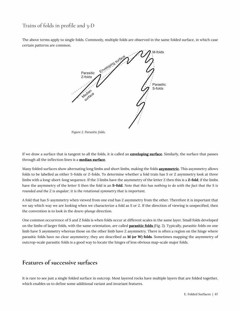
Trains of folds in profile and 3-D

The above terms apply to single folds. Commonly, multiple folds are observed in the same folded surface, in which case

certain patterns are common.

Figure 2. Parasitic folds.

If we draw a surface that is tangent to all the folds, it is called an enveloping surface. Similarly, the surface that passes

through all the inflection lines is a median surface.

Many folded surfaces show alternating long limbs and short limbs, making the folds asymmetric. This asymmetry allows

folds to be labelled as either S-folds or Z-folds. To determine whether a fold train has S or Z asymmetry look at three

limbs with a long-short-long sequence. If the 3 limbs have the asymmetry of the letter Z then this is a Z-fold; if the limbs

have the asymmetry of the letter S then the fold is an S-fold. Note that this has nothing to do with the fact that the S is

rounded and the Z is angular; it is the rotational symmetry that is important.

A fold that has S-asymmetry when viewed from one end has Z asymmetry from the other. Therefore it is important that

we say which way we are looking when we characterize a fold as S or Z. If the direction of viewing is unspecified, then

the convention is to look in the down-plunge direction.

One common occurrence of S and Z folds is when folds occur at different scales in the same layer. Small folds developed

on the limbs of larger folds, with the same orientation, are called parasitic folds (Fig. 2). Typically, parasitic folds on one

limb have S asymmetry whereas those on the other limb have Z asymmetry. There is often a region on the hinge where

parasitic folds have no clear asymmetry; they are described as M (or W) folds. Sometimes mapping the asymmetry of

outcrop-scale parasitic folds is a good way to locate the hinges of less obvious map-scale major folds.

Features of successive surfaces

It is rare to see just a single folded surface in outcrop. Most layered rocks have multiple layers that are folded together,

which enables us to define some additional variant and invariant features.

E. Folded Surfaces | 67

In profile

A line drawn through all the hinge points of a fold is called the axial trace of the fold. (It’s also called the hinge trace,

which is arguably a better term because the trace has little relation to the fold axis, but most structural geologists use

axial trace.)

The other variant and invariant points also correspond to traces on the profile plane: inflection trace, crest trace, trough trace. (Because all these lines are the traces, on the profile plane, of surfaces in 3-D, the word ‘surface’ is

sometimes added: inflection surface trace, crest surface trace, trough surface trace.)

Figure 3. Features of multiple folded surfaces.

68 | E. Folded Surfaces

In 3-D

By now you can anticipate that in 3-D each of the lines that we identified on a single surface can be extrapolated into a

surface in 3D.

The most important surface is the axial surface (or hinge surface). This surface is of great kinematic significance

because the pole to the axial surface is often the direction of maximum shortening.

The other surfaces: inflection surface, crest surface, and trough surface are all parallel to the axial surface in a

cylindrical fold.

The facing direction is the direction of younging in the fold axial surface. It is perpendicular to fold hinges but lies in the

axial surface. Notice that folds may have overturned limbs but still face upward.

The relationship of facing direction to anticlines, synclines, antiforms, and synforms:

ANTIFORM SYNFORM

ANTICLINE Antiformal anticline Synformal anticline

(Upward facing) (Downward facing)

SYNCLINE Antiformal syncline Synformal syncline

(Downward facing) (Upward facing)

Notice that in upward facing folds the ‘-form’ and the ‘-cline’ are the same. In downward facing folds the ‘-form’ and

‘-cline’ are different.

Fold attitude

Because of its kinematic significance, the strike and dip of the axial surface are important features to measure in an

outcrop of a fold. Folds can be classified by axial surface orientation:

Dip Classification by axial-surface dip

0-10° Recumbent

10-30° Gently inclined

30-60° Moderately inclined

60-80° Steeply inclined

80-90° Upright

Because of the way the axial surface is defined, the hinge of a fold must be a line that lies in the axial surface. This means

that the plunge of the hinge cannot be steeper than the dip of the axial surface. It also means that the hinge line has a

rake or pitch in the axial surface. There is a special term for folds in which the rake of the hinge in the axial surface is

close to 90°: these are reclined folds.

E. Folded Surfaces | 69

Figure 4. This is a rounded, upright, subhorizontal, open, upward facing, synformal syncline. Bramber, Nova Scotia.

Figure 5. Moderately inclined, tight, antiformal anticline. David Thompson Highway, Alberta.

Figure 6. Steeply inclined folds with axial planar cleavage. Carmanville, Newfoundland.

Figure 7. Recumbent fold. Picadilly, Newfoundland.

Figure 8. Variably inclined synform. Port au Port Peninsula, Newfoundland.

Harmonic and disharmonic folds

All the above features are characteristic of folds where each layer is folded in step with the adjacent layers. These are

called harmonic folds. Sometimes we find layered rocks in which the folds are not so aligned. These are disharmonicfolds. It’s not usually possible to define axial, inflection, trough, or crest surfaces in disharmonic folds, which therefore

provide less information about regional deformation than harmonic folds.

70 | E. Folded Surfaces

Figure 9. Buckle folds in sandstone. Rainy Cove, Nova Scotia. Figure 10. Kink band in slate. Tancook Island, Nova Scotia.

Figure 11. Refolded isoclinal folds, Pond Point, Bay of Islands, Newfoundland.

Some common fold styles

Some types of fold style occur in many circumstances, and can give clues as on the dynamics of folding.. Where layers

of strong rock are interlayered with very weak rock, the strong layers may have nearly constant thickness around fold

hinges, so that the inner and outer arcs are parallel. Such folds are called parallel or concentric folds. Distinctive styles

of parallel folds occur when the strong layers are close together and can slide over each other easily. Under these

conditions, very angular folds may develop. When these have inter-limb angles around 60° they are called chevron folds.

Inter-limb angles around 120° define kink folds. Conversely, when all the layers are weak, for example in rocks near

their melting point, folds may develop in which each folded surface is geometrically similar to the next; these are similar folds.

Figure 12. Styles of fold. (a) Parallel folds produced by buckling. (b) Similar folds. (c) Chevron folds. (d) Kink folds.

E. Folded Surfaces | 71

Folds in map view

Folded rocks are more complicated in map view than simple planar strata, because map patterns result from a

combination of hills and valleys in the landscape, and antiforms and synforms in the strata.

The shape of folded strata can often be figured out with structure contours, but unlike those for simple planar strata,

structure contours for folded strata are not straight. They show angles or curves. Some examples are shown in the

following diagrams.

If the fold hinges are perfectly horizontal, the structure contours will remain straight and parallel, but the numbers will

show changes of dip:

Figure 13. Structure contour pattern for a horizontal antiform.

However, if the fold plunges, the contours themselves will V-shaped, in the case of an angular fold:

72 | E. Folded Surfaces

Figure 14. Structure contour pattern for a plunging angular synform.

If the fold is rounded, the structure contours will be curved, showing U-shapes:

Figure 15. Structure contour pattern for a plunging rounded antiform.

If the fold is overturned, the contours will again be V or U-shaped but contours for both limbs will occur on the same

side of the fold hinge:

E. Folded Surfaces | 73

Figure 16. Structure contour pattern for an overturned plunging angular synform.

Fold overprinting

Areas affected by multiple episodes of folding may display refolded folds in a bewildering variety of orientations,

producing a variety of fold interference patterns.

Classification of fold interference patterns

To make sense of these we use a classification (devised, like many other fundamental classifications of folds, by J.

Ramsay, 1967). This classification relates to two generations of folds only – if we have 3 or more generations things get

more complicated.

In each case we characterize a first generation of folds by

• an axial surface

• a fold hinge that lies in that axial surface

We examine the effect of the second generation of folds on those two structures.

74 | E. Folded Surfaces

Figure 17. Type 0 fold interference pattern.

Figure 18. Type 1 fold interference pattern.

If later folding does not bend either the axial surfaces or the hinges of early folds,

then the early folds are effectively just tightened during the second phase of

deformation. The fold pattern is described as ‘type 0’, and generally it will not be

apparent from geometry that there have been two phases of deformation.

If later shortening is roughly parallel to the hinges of the early folds, and the

extension direction also lies in the early fold axial surfaces, then later folding

bends the hinges of the early folds but does not significantly bend the axial

surfaces. This typically produces culminations and depressions on the early fold

hinges, and leads to oval outcrop patterns of layer traces on outcrop surfaces.

This is called a type 1 fold interference pattern, characterized by domes and

basins.

E. Folded Surfaces | 75

Figure 19. Type 2 fold interference pattern.

Figure 20. Type 3 fold interference pattern.

If on the other hand, the extension direction in the second deformation is at a

high angle to the early axial surfaces, then those axial surfaces may be folded too.

Under these circumstances outcrop patterns are characterized by complex

shapes that resemble mushrooms and bananas. This is called a type 2 interference

pattern.

There is a third case, which occurs when the shortening direction is at a high

angle to the early fold hinges and the extension direction is at a high angle to the

early axial surfaces. Under these conditions the early hinges may remain more or

less straight but the early axial surfaces are folded. The trace of layering typically

follows a multiple zigzag shape described as a type 3 interference pattern.

76 | E. Folded Surfaces

Figure 21. Interpretation of fold interference patterns.

How to analyse an overprinted fold pattern

When trying to understand an overprinted fold pattern,

the most important first step is to draw axial traces. In

general, the latest set of axial traces is likely to be

approximately straight. Earlier axial traces may or may

not be folded. (In general, type 1 interference patterns,

where early axial surfaces are not folded, are the most

difficult to analyze; it may not be possible to determine

the order of folding.)

Facing directions may also be useful in the analysis of

overprinted folds. For example, downward-facing folds

(synformal anticlines and antiformal synclines) always

indicate that there are at least two generations of folds.

References

Davis, G.H., Reynolds, S,J. and Kluth, C.F. (2011) Structural Geology of Rocks and Regions, 3rd Edition, Wiley, New York.

Ramsay, J.G. (1967) Folding and Fracturing of Rocks: San Francisco, McGraw Hill, 568 p.

Van der Pluijm, B.A. & Marshak, S. (2004) Earth Structure, Norton, New York.

E. Folded Surfaces | 77

• Lab 4. Introduction to Folds

Map techniques for folds

Both contouring and stereographic projection are powerful techniques for the analysis of folds. When contouring folded

surfaces, you may have to try out more than one possible solution. Map patterns in folded rocks may show V-shapes that

represent true fold hinges, and other V-shapes that represent the effect of valleys and ridges intersecting with planar

surfaces. Try to identify any V-shapes that cannot be attributed to topography; these are likely to be outcrops of fold

hinges. Fold hinge outcrops lie on fold axial traces. These are lines on the map that divide the map into different fold

limbs. Try to work on one limb at a time when contouring. Remember, there may be more than one possible solution,

but the simplest solution, geologically, is usually the best.

If a fold is cylindrical, then all the planes in the folded surface contain the same line. In principle, if we find the

intersection of any two planes, we can define the fold axis. The plane perpendicular to the fold axis is the profile plane.

We can also use the stereographic projection to find the inter-limb angle, if we have measurements of the orientation

of the folded surface on the limbs at the inflection points.

Assignment

Do the questions in any order, so as to use the various materials when they are available. (Samples for question 1 may

not be available outside the lab hours.)

1.* Look at the samples of folded rocks displayed in the lab. Choose one sample in each group, and make a labelled

diagram of the fold in profile view. Make your diagram large (fill a whole page). Your diagram should be a scientific

illustration, not a work of art! Use simple clear lines to show boundaries of layers within the sample. If there are too

many layers to show precisely, use a dashed ornament to show the form for the layer traces. Label as many invariant

features as you can.

2.* Why would you not label variant features of these folds?

3. Construct a topographic profile and cross-section through Map 1. Proceed as follows. Mark with colours the various

surfaces that separate the units. Look for places where V-shapes in the traces cannot be explained by valleys and

ridges in the topography, and lightly circle possible locations for fold hinge points. Draw structure contours for

each surface, on each fold limb, using lead pencil. Use coloured numbers on the contours, to show which contour

corresponds to which surface. Use these to construct the geology on the cross-section.

4. Describe the folds as completely as you can using the terms in the previous sections of this manual. (Note that the

units are shown in their correct stratigraphic order in the legend.)

Lab 4 Map 1 Folded rocks

5. Examine the map of the Great Cavern Petroleum prospect.

a) Draw structure contours on the fault surface.

Lab 4. Introduction to Folds | 79

b) Contour the top surface of the Great Cavern Limestone. In the southeast of the map, use the intersections of

the outcrop trace with the contours. Elsewhere, use the elevations marked against each of the 26 dry oil wells.

Make your contours as smooth as possible, consistent with the data provided. (Make the contours as smooth

as possible in 3 dimensions too: this means that the spacing of contours should be as even as possible on each

fold limb.) Mark the position of any fold hinges, and draw hinge lines. Remember that top limestone structure

contours will be cut off by fault structure contours of the same elevation.

c) *Calculate the plunge and trend of the easternmost fold in the area. Keep a note of your answer as you will need

it in lab 5.

d) *Construct cross-section A-B

e) Construct cross-section C-D

f) On the map, and on cross-section C-D, show the potential maximum size of an oil reservoir that might have been

missed by the existing wells. (Note that in porous units like the Great Cavern Limestone, oil usually rises to the

highest point in the reservoir rock; the base of an oil reservoir is typically a horizontal oil-water contact.) Draw

the maximum extent of the potential reservoir on the map and the cross section. Suggest a spot for well 27 on

the map and cross section which would maximize the chance for an oil discovery.

g) *Make an estimate of the maximum potential volume of the reservoir, if the Great Cavern Limestone has 10%

porosity. To do this, estimate the maximum possible area of the reservoir in square metres. Also calculate its

maximum vertical thickness. Then, by approximating the shape of the reservoir as a cone, use the equation for

the volume of a cone (one third base area times height) to figure out the approximate volume of the reservoir,

and from this, a rough estimate of the maximum volume of petroleum it might contain.

(For a more realistic estimate of the potential resource it would be necessary to take into account the potential

presence of other fluids in the reservoir, the effects of pressure, and the proportion of the fluids that could be

economically extracted.)

h) *Research: find out the conversion factor between cubic metres and barrels, and express your answer in barrels!

Lab 4 Map 2 Great Cavern Map

80 | Lab 4. Introduction to Folds

Figure 1. Principle of the pi-diagram, to find the fold axis of a cylindrical fold from measurements of folded surfaces.

• Lab 5. More about Folds

Multiple planes on the stereographic projection

The techniques you used in the last lab work well for folds

that are perfectly cylindrical, and where the orientations

of the folded surfaces are known with great precision.

However, in many cases, folded surfaces are not perfectly

cylindrical, and small variations in dip, and measurement

errors, mean that the geometry is not perfect. Under

these circumstances, to determine the orientation of a

mean fold axis, it is desirable to measure a large number

of orientations, and to use a statistical approach.

Unfortunately, plotting large numbers of great circles

rapidly produces a very cluttered projection. For this

reason, it is much better to plot poles to the folded

surfaces rather than great circles. In the ideal case the

poles should all lie in the profile plane, and therefore they

will plot as points on a single great circle. In real life,

things are not so simple; the poles appear scattered in a

band, or girdle, on either side of the profile plane, which

has to be estimated as a ‘best-fit’ great circle through the

densest band of points.

There is an additional problem, however. If you look at the

Wulff net, you will see that the 2° and 10° squares project

much larger near the primitive than they do at the centre

of the net. This means that plots made with the Wulff net

should never be used for statistical inferences based on

density of points, bcause it artifically increases the

density in the centre and decreases it on the primitive.

More About Folds | 81

Schmidt net, for plotting equal area projections

For this reason, a modified stereographic projection, called

the equal area projection is used, based on the Schmidt net. All

the operations you have met so far are the same on the two

nets; the only difference is that the equal area projection does

not preserve circular arcs – the great and small circles are

complex curves and cannot be drawn with a compass. For this

course make sure your net is printed so that its diameter is exactly 15 cm.

Pi diagram

The resulting plot of poles to planes on a equal area projection

is called the pi-diagram, which is the most common method

used to find the mean fold axis in an area of folded rocks where,

as often happens, individual fold hinges are not exposed. The

principle of the pi-diagram is illustrated in Figure 1. In a

cylindrical fold, the poles to the folded layers are lines perpendicular to the fold axis. They therefore lie in the profile plane, the plane that is perpendicular to the fold axis. If the folds are not perfectly cylindrical, or if there are small errors

in the measurements, the lines will not lie precisely in the profile plane, but will be close to it.

Contours on the axial surface

Maps of areas with folded rocks can be challenging because of the number of surfaces involved, and because of rapid

changes of strike and dip. Often, even though layers may show complex folding, axial surfaces may be approximately

planar. Under these circumstances it makes sense to separate the limbs of the fold by drawing axial traces, and even

to draw contours on the fold axial surfaces. When doing this, it’s important to remember that a single fold will have

multiple hinges (one for each folded surface), but that these hinges lie in a single fold axial surface.

Assignment

1.* The area you contoured last week (Great Cavern petroleum prospect) shows strike and dip symbols representing

measurements of bedding orientation.

Plot poles to bedding for all the strike and dip measurements on an equal area projection, to make a pi-diagram.

Find and draw the best-fit great circle through the poles; this represents the profile plane. Mark the best

estimate of the fold axis (pole to the profile plane) and determine its trend and plunge. Is it similar to the value

you obtained by contouring last week, and to the values obtained by your other team members?

Lab 4 Map 2 Great Cavern Map

82 | More About Folds

2.* Look at the map of Somerset County in the Appalachians of Pennsylvania. The area has a long history of coal mining,

and a number of coal seams are identified on the stratigraphic column that doubles as a legend.

a) The map has structure contours, shown in red, drawn on one surface. Which one surface? (Note: each formation

on the map has a top and a bottom surface, so just a formation name is not a complete answer; your answer

should be in the form ‘the boundary between Formation x and Formation y’.)

b) Use the spacing of the structure contours to determine the strike and dip, at its steepest point, on each limb of

the most conspicuous fold. Note that the contours are in feet, and the scale of the map is 1:62500 (about 1 inch

to 1 mile). Make sure that in your dip calculation you use the same units vertically and horizontally. Use the points

where the contours cross the fold hinge to determine the average trend and plunge of the fold hinge.

c) Plot both limbs of the fold from part ‘b’ on a stereographic projection. Using the intersection and the angle

between the planes, estimate the plunge and trend of the fold axis, and the interlimb angle of the fold.

d) Based on these observations, describe the orientation (plunge, tightness, overall orientation) of the fold in words

(e.g. ‘tight, steeply plunging synformal anticline’)

e) If the fold is cylindrical, the fold axis orientation determined stereographically should coincide with the hinge

orientation determined by contours. How close are they (in degrees)?

To find out more, take a look at: Flint 1965 Geology and mineral resources of southern Somerset County, Pennsylvania

3. Map 1 contains an angular fold in a more general orientation than the perfectly horizontal folds you dealt with

last week. In addition there are some unfolded rocks and an intrusion. An unconformity separates the more highly

deformed folded rocks from the gently dipping younger rocks. To help you solve the map, note that in the west of

the map, the bedding traces are somewhat parallel to the topographic contours. These regions correspond to a gentle

fold limb. Elsewhere, the geological boundaries cut across the contours at a steeper angle; this is a steep fold limb.

Fold hinges can also be identified on the map from sharp swings in the trace of bedding that are not obviously related

to valleys and ridges. Before you begin, try to use these hinges to sketch where there might be fold axial traces; these

More About Folds | 83

should separate regions of steeper and more gently dipping beds. Do this very lightly – it is likely you will change your

mind as you proceed.

a) Identify the various surfaces on the map. First, mark the unconformity surface in green or yellow. Then mark the

boundary between marble and amphibolite in blue or violet. Mark the boundary between amphibolite and schist

in red or orange. (Note: the colour scheme is provided for convenience. If you choose different colours, you must

use them consistently throughout this exercise.)

b) Draw structure contours on the green surface.

c) Draw structure contours on the red surface. You will find that there are two parts to this surface: a steep limb

and a gentle limb. These have separate sets of contours. The two sets of red contours intersect in a fold hinge.

Mark this on the map and trace over it with red.

d) Repeat for the blue surface and mark the blue hinge.

e) The red hinge and the blue hinge are both lines that lie in the axial surface of the fold. Join points of equivalent

elevation on the red hinge and blue hinge with lines: these are structure contours on the axial surface. Number

them in purple or violet.

f) Use the axial trace contours to predict the outcrop trace of the axial surface, and draw this trace on the map. The

axial trace should separate the steep limb from the gentle limb of the fold.

g) Make a cross section along the line XY.

h) Plot both fold limbs, the axial surface, and the unconformity as great circles on an equal area projection. Mark

the point corresponding to the orientation of the fold axis.

i) Describe the orientation of the fold in words as completely as you can

j) List the events in the geological history of the area for which you have evidence, starting with the oldest. In the

case of the three folded units, where there is no direct evidence of age, you should assume that the fold is upward

facing (i.e. synforms are also synclines; antiforms are also anticlines).

Lab 5 Map 1 Folded area

Schmidt Net 15 cm

84 | More About Folds

Figure 1. Boudinage. Top: boudins; bottom: chocolate tablet structure.

F. Boudinage

Buckle folds are formed when strong (or ‘competent‘)

layers of rock are shortened. What happens when strong

layers are extended? Typically the layers start to thin at

points of weakness (a process known in engineering as

necking) producing a structure called pinch-and-swell.As pinch and swell develops, the thin regions can

separate, leaving a structure that looks like a string of

sausages in cross-section. The remnants of the original

layer are called boudins (a French word for a type of

sausage), and the process is known as boudinage.

Although boudins are in many ways the extensional

counterpart of folds, the terminology of boudinage is

much less well developed that of folds. In part, this is

because layers undergoing boudinage do not affect

adjacent layers in the same way, so that boudins are less

likely to be harmonic than folds. Thus, although boudins

do have axes, it is rarely possible to define an equivalent

of an axial surface for boudins.

Sometimes layers undergo extension in all directions simultaneously, producing a more three-dimensional boudinage

structure described as chocolate tablet structure. It is also possible to find examples of layers that have undergone both

folding and boudinage during progressive deformation.

Figure 2. Boudins formed from quartz vein. Carmanville, Newfoundland.

F. Boudinage | 85

Figure 1. Four parts of deformation.

G. Kinematic Analysis and Strain

Everything we have done so far in this course has been about describing the ‘here and now’ of structural geology: where

are structures and how are they oriented in the Earth’s crust at the present day.

To understand the origin of structures we need to know how things changed during the formation of those structures –

how things moved. When we study how things moved over geologic time, we are studying kinematics.

The basic movements

Deformation can involve 4 types of movement:

• Translation, or change in position

• Rotation or change in orientation

• Dilation or change in area or volume

• Distortion or change in shape.

The first two are rigid body deformations. The last two

together constitute non-rigid deformation or strain.

Translation

Translation is measured as a displacement. Any

displacement has a distance and a direction. When we

look at faults we will measure the displacement of one

wall of a fault relative to another. Displacement is a vectorquantity.

Rotation

Rotation, or change in orientation, is typically measured in degrees, about a particular axis of rotation. (A rotation is

therefore also a vector quantity, because it has a magnitude and a direction.)

A common kinematic problem involving rotation is to remove the effects of folding from some structure. For example,

a sedimentologist may measure the orientation of a paleocurrent structure in folded strata, and wants to know the

original direction of current flow.

This type of problem is most easily solved on the stereographic projection. As beds are ‘unfolded’, the paleocurrent

directions they contain rotate along small circles on the stereonet. The small circles are centred on the fold axis.

G. Kinematic Analysis and Strain | 87

Dilation

Volume change is very difficult to measure in real rocks. However, under some circumstances it can be quantified. Most

sedimentary rocks undergo some compaction as they are buried, because pore water is expelled. Compaction results

in a negative dilation. Another common phenomenon involving negative dilation is pressure solution in which some

minerals in a rock are dissolved in response to stress.

Dilation is a scalar quantity – it just has a magnitude.

Distortion

Distortion is by far the most complicated type of deformation to measure. When rocks are distorted they typically get

longer in some directions and shorter in others. Also, angles change in distortion. Because of this, strain cannot be

represented by a scalar or a vector. It is a more complicated quantity that is called a tensor.

Strain

In popular speech the word “strain” conjours up an impression of applying force; “straining” at something implies a

dynamic process. The word “strain” has a different meaning in science and engineering – it describes something purely

kinematic – a change in shape or volume, however caused. There are examples of strain in which no force is involved: A

reflection in a distorting mirror, and the distorted image of a basketball on a widescreen TV are both images that have

undergone strain, but they are made of light rays; no force is causing the distortion.

(The corresponding dynamic term is “stress”, which we will study in a later section. Take care never to confuse stress

with strain!)

All the structures we see in the Earth’s crust are manifestations of strain. Strain is such a fundamental concept in

structural geology that in more advanced courses, the mathematics of strain is often treated first. In this course we take

a more practical approach and focus on describing structures first. However, by now, it should be clear that changes in

the shape of rocks can be recognized in all the structures you have studied so far.

Heterogeneous strain and homogeneous strain

Strain can vary from place to place in rocks. We distinguish a special case:

Homogenous strain: strain that is the same everywhere within a body of rock. In homogeneous strain, straight lines

remain straight, parallel lines remain parallel, circles are deformed into ellipses.

Strain that is not homogeneous is heterogenous. In heterogenous strain, straight lines can be bent, and lines that were

initially parallel are rotated by different amounts, becoming non-parallel.

88 | G. Kinematic Analysis and Strain

Heterogeneous strain is difficult to deal with mathematically. However, if we look at a very small region of a

heterogeneously strained rock, it can often be treated in the same way as a homogeneous strain. The strain at a point in a heterogeneously strained rock follows the same mathematical rules as homogenous strain.

Figure 2. Homogeneous and heterogeneous strain.

G. Kinematic Analysis and Strain | 89

Figure 3. Strain affecting variably oriented trilobites. Note that each fossil is affected differently, depending on its initial orientation but the strain is nonetheless homogeneous. Trilobite image after Gon, S.; www.trilobites.info; Downloaded 2012 Dec 17.

Strain along lines

Even in a homogeneous strain, differently oriented lines experience different amounts of strain. In the diagram, each

trilobite is affected differently by deformation, even though the overall strain is homogeneous.

90 | G. Kinematic Analysis and Strain

Figure 4. Longitudinal strain as it affects the mid-line of one trilobite in Figure 3.

Figure 5. Shear strain as it affects the mid-line of one trilobite in Fig. 3.

Changes in length (longitudinal strain)

There are two ways to measure change in length. If

original length is l0 and new length is l,

Extension (sometimes elongation) e = (l-l0)/l0

Extension is the fractional change in length.

Stretch s = l/l0 = 1+e

The important thing to remember is that in strained rocks

the elongation varies with direction: typically some lines

will have got longer and others will have got shorter.

Changes in angles (shear strain)

To measure change in angles we look at two lines that

were originally perpendicular.

If the change in angle is ψ (psi) then

Shear strain (gamma) γ= tan ψ

There are other methods used to measure shear strain in

advanced studies, so the above definition is sometimes

qualified as engineering shear strain because it is the

measure allegedly most used by engineers.

Shear strain also varies with direction – some lines

undergo positive shear strain and some undergo negative

shear strain.

In the diagram, the long axis of the trilobite has

undergone positive shear strain because the line originally perpendicular to it has rotated relatively clockwise.

G. Kinematic Analysis and Strain | 91

Figure 6. (a) Strain ellipse; (b) strain ellipsoid.

Strain ellipse

The strain ellipse is a convenient way to represent a state

of homogenous strain, or the strain at a point, on a two-

dimensional surface. The strain ellipse is the shape of a

deformed circle that originally had unit radius.

The radius of the strain ellipse in any direction is equal to

the stretch s in that direction. The strain ellipse is thus a

good way to represent the variation of longitudinal strain

with direction.

Strain axes

A strain ellipse has two lines that are special. They

represent the maximum and minimum stretches. These

lines are strain axes. (The strain axes are sometimes called X and Z. (Note: coordinate axes on a map or cross-section

are sometimes x and z. Strain axes don’t necessarily coincide with any special direction on a map.)

Strain axes have some other special properties. They are always at right angles to each other, and they also represent

lines of zero shear strain. This means that they were perpendicular before deformation started too. (However, during

deformation they may have diverged from this perpendicular relationship and then come back to it!). The strain axes are

the only lines that have this property.

The strain ratio is a convenient measure of the amount of distortion in 2-D. The strain ratio is the ratio between the

long axis and the short axis of the strain ellipse:

Strain ratio RS = sX/sZ

Strain ellipsoid

The strain ellipsoid is a convenient way to represent a state of homogenous strain, or the strain at a point, in three

dimensions. The strain ellipsoid is the shape of a deformed sphere that originally had unit radius.

The radius of the strain ellipsoid in any direction is equal to the stretch s in that direction. In 3-D, the strain ellipsoid is

thus a good way to represent the variation of longitudinal strain with direction.

A strain ellipsoid has three lines X,Y and Z that are special. They represent the maximum and minimum stretches, called

sX and sZ respectively, and a third, intermediate axis of intermediate stretch sY, that is mutually perpendicular to the

other two. These lines are strain axes.

They have some other special properties. They are at right angles to each other, and they also represent poles to

planes of zero shear strain. This means that they were perpendicular before deformation started too. (However, during

deformation they may have diverged from this perpendicular relationship and then come back to it!). The strain axes are

the only lines that have this property.

92 | G. Kinematic Analysis and Strain

In 3D the strain axes are poles to three principal planes of strain.

In 3D the shape of the strain ellipsoid can’t be defined by a single strain ratio. Instead we recognize two strain ratios a=

sX/sY and b= sY/sZ. If a is large and b is small then the strain ellipsoid looks like a football or a cigar, and is described as

prolate. Rocks with prolate strains often display strong linear fabrics (lineations). In contrast if a is small and b is large

then the strain ellipsoid looks like a cushion or a pancake, and is described as oblate. Rocks with oblate strains often

display strong planar fabrics (foliations).

The range of possible strain ellipsoid shapes can be illustrated on a graph of a against b known as a Flinn plot.

Deformation histories

Rotational and non-rotational deformation

All the above measures have concerned just strain. However, if we look at the whole deformation picture, we may see

situations where rotation has gone on at the same time as strain. Under these circumstances it’s helpful to look at the

behaviour of the strain axes.

If the strain axes have the same orientation as they did before deformation started, then the deformation is non-rotational (sometimes irrotational). (Note that even in a non-rotational strain other lines will have been rotated, and

will show shear strain, but it is the strain axes that are important for the terminology here.)

If the strain axes have rotated during deformation, then the deformation is described as rotational.

Finite deformation and deformation rate

Once we start looking at rotation, it’s difficult to avoid discussing strain history too. When we look at a deformed rock

what we see is the product of a whole history of deformation. That end product is called the finite deformation and the

strain part of the deformation is the finite strain.

In more detailed analyses of strain, we may be interested in all the tiny increments of strain that have contributed to

the final picture. Each one is called an incremental strain.

The infinitesimal strain is the end product of this type of thinking. The strain history is thought of as being made up

of an infinite number of infinitesimal strain increments. (The general idea should be familiar if you have taken a class

in calculus.) This idea of infinitesimal strain becomes important if we look at strain rates. Strain rates are typically

measured in units of strains per second or s-1. In geologically reasonable situations, the amount of strain that occurs in

a second is almost infinitesimal. Typical ductile strain rates in the Earth’s crust are thought to be between 10-12 and 10-15

s-1.

G. Kinematic Analysis and Strain | 93

Coaxial and noncoaxial deformation histories

If the strain increments are all non-rotational, then the strain axes maintain their same direction relative to the material

of the rock. The deformation is called coaxial. This type of deformation is also called pure strain.

Any other type of strain history is a noncoaxial. There are many types of noncoaxial strain history, but one particular

type is important in the study of shear zones. It is simple shear. In simple shear, all the particles of the rock move in

the same direction, but the strain axes are progressively rotated. Sometimes, by looking in detail at the fabric of shear

zones, we can distinguish the sense of rotation and figure out which way the rocks were moving.

94 | G. Kinematic Analysis and Strain

H. Fabrics

Introduction: foliations and lineations

Any rock that has properties that vary with direction is said to have fabric. Like most structures, fabrics can

be primary or secondary. Examples of primary fabric are bedding in sedimentary rocks and flow banding in igneous

rocks. Secondary fabrics typically indicate that strain has occurred. Fabrics are common in folded rocks, and if fabrics

develop at the same time as folding they often have a very specific relationship to folds.

Fabrics may be planar or linear. Planar fabrics are also called foliations. (Note that some textbooks restrict the term

foliation to particular types of planar fabric, with coarse mineral grains as in a schist; we will use it in a more

general sense to designate any planar fabric.) Rocks with a strong secondary planar fabric are sometimes called S-tectonites (the S is for schistosity). Linear fabrics are called lineations. Rocks with a strong secondary lineation are

sometimes called L-tectonites.

It is common to find a lineation that lies parallel to (or in the plane of) a planar fabric. Rocks with a strong tectonic

lineation that lies in the plane of a tectonic foliation are sometimes called LS-tectonites.

Fabric Elements

Fundamental to the description of fabrics is the concept of a fabric element. Fabric elements (Fig. 1, 2) are the things that are aligned to give a rock a fabric. Fabric elements include things like layers and lenses of different composition, grains

of minerals that are tabular (like mica) or acicular (like hornblende or sillimanite). Folds can also be fabric elements, if

there are enough of them.

This leads to a second important concept: the idea of a penetrative fabric. A fabric is penetrative if it is present

everywhere in the rock. For example, some slates can be split almost anywhere: there’s effectively an infinite number of

cleavage planes. In others, the cleavage planes are visibly spaced and are termed non-penetrative.

Penetrative fabrics

A fabric is penetrative if:

• It is present throughout the rock,

• It is not possible to count the number of fabric planes or lines,

• It is not possible to see spaces between the fabric planes or lines.

H. Fabrics | 95

Figure 1. Different types of foliation and their fabric elements. In each case the foliation is parallel to the top surface of the block. (a) Compositional layering; (b) grain size variation; (c) closely-spaced fractures; (d) preferred orientation of grain boundaries; (e) preferred orientation of domains of different composition; these domains could be mineral grains, groups of mineral grains, deformed pebbles, etc. These various types of fabric element can be combined. ( f) A combination (a + e) that is common in sedimentary and metamorphic rocks. Based on Hobbs, B.E., Means, W.D., and Williams, P.F. 1976. An Outline of Structural Geology. Wiley.

Non-penetrative fabrics

A fabric is non-penetrative if:

• The fabric planes or lines are spaced apart within the rock,

• It is possible to see spaces between the fabric planes or lines where no fabric is present,

• The fabric planes or lines can be counted.

Note that penetrative character is a scale-dependent concept; a fabric that is penetrative at map and outcrop scale may

prove to be non-penetrative in thin section.

Fabric elements

The following types of fabric elements can give a rock a

fabric. Notice that it’s common for a given fabric to be

defined by a combination of fabric elements, as shown in

Figures 1 and 4.

Tabular mineral grains:

Platy or flake-shaped mineral grains like mica are

often aligned to produce a foliation.

Less obviously, tabular mineral grains may

contribute to lineation if their orientations are

scattered so that their planes all include a

particular line.

Acicular mineral grains:

Needle-shaped, or acicular, mineral grains like

amphibole and sillimanite are often aligned to

produce a lineation.

Less obviously, needle-shaped mineral grains may

contribute to foliation if they are distributed

parallel to a plane.

Crystallographic preferred orientation (CPO):

Sometimes it is necessary to look at thin section

under the microscope to see a fabric. If the

crystallographic axes of a particular mineral are all

parallel to a particular plane or line, then the rock

has a fabric. Typically this will only become

obvious when the microscope stage is rotated

between crossed polars, especially when a

1-lambda plate is inserted; all the grains change colours ‘in sync’ as the stage is rotated.

96 | H. Fabrics

Figure 2. Sedimentary foliation: bedding and fissility, Arisaig, NL.

Domains:

A domain is a region within a rock that has a distinctive composition or texture. Flattened clasts in a sedimentary

rock can produce a foliation if they are all aligned to a plane. Stretched clasts in a sedimentary rock can produce

a lineation if they are all aligned parallel to a line.

Layers:

Layers are really just domains that are very extensive and parallel-sided.

Rods:

Rods are really just domains that are very elongated and continuous.

Cracks and discontinuities:

Closely spaced fractures can produce a type of cleavage called fracture cleavage.

Fold hinges:

Numerous closely spaced fold hinges may produce a lineation in highly deformed rocks. This structure is called

a crenulation lineation.

Fold axial surfaces:

Numerous closely spaced fold axial surfaces may be planes of weakness in highly deformed rocks. This structure

is called crenulation cleavage.

Intersecting foliations:

Whenever two intersecting foliations are present, there is always an intersection lineation defined by their

intersection. In the field, although it’s possible to calculate the intersection lineation from strike-and-dip

measurements of the two foliations, it’s usually much more accurate to measure the lineation directly.

Common types of foliation, and their origins

Primary fabrics:

Sedimentary rocks are typically recognized by their primary

fabrics. Actually, two types of fabric are common:

1. Bedding and lamination are defined by layers of different

composition or texture, typically reflecting environmental

change during deposition;

2. Fissility is a fabric characteristic of mudrocks, in which

the sheet silicates have been aligned by compaction to

produce a penetrative primary foliation.

H. Fabrics | 97

Figure 3. Axial planar slaty cleavage parallel to hammer handle, Carmanville NL.

Slaty cleavage:

Slaty cleavage is a penetrative fabric in which micas or other

sheet silicates, below the limit of visibility with the naked eye,

are aligned parallel to a plane, which becomes an easy plane of

splitting. Strain studies have shown that slaty cleavage typically

forms perpendicular to the direction of maximum shortening,

the Z axis of the strain ellipsoid. In other words, cleavage forms

parallel to the X-Y plane. Some slaty cleavages are penetrative

down to the scale of individual mineral grains; others show

domains under the microscope.

Cleavage is thought to develop by a combination of processes

including:

1. Physical rotation (transposition) of mineral grains as a rock

is deformed;

2. Solution of grains subjected to high stress (pressure

solution);

3. Growth of new mineral grains during deformation.

Slaty cleavage is the defining characteristic of the rock-

type slate.

Schistosity:

Schistosity is a coarser grained version of slaty cleavage, and is

the term used for a more or less penetrative foliation defined by mineral grains coarser than about 1 mm. Many

geologists actually recognize an intermediate feature phyllitic foliation, when the fabric-defining minerals are just

visible. However, the boundaries between these categories have never been formally defined.

Schistosity involves the same types of process as slaty cleavage, but is typical of higher metamorphic grades and always

involves significant new mineral growth.

Gneissic banding:

Gneissic banding is developed as a result of recrystallization during medium- to high-grade metamorphism. It is

characterized by the preferred orientation of platy, tabular, or prismatic minerals, and by subparallel lenticular mineral

grains and grain aggregates. Most gneisses also display compositional (mafic/felsic) banding.

Flattening fabric:

When a foliation is defined by domains that represent identifiable deformed objects in a rock, such as flattened pebbles

in a deformed conglomerate, the fabric can be called a flattening fabric. (Most foliations are probably produced by

flattening, but this term is used when the origin is obvious.)

98 | H. Fabrics

Figure 4. Pressure-solution cleavage, Bay of Islands NL.

Pressure-solution cleavage:

Sometimes deformed rocks contain domains or layers of

different composition that can be shown to have

originated as a result of solution of particular minerals.

For example, quartz may be preferentially dissolved from

certain bands within a rock, producing mica-rich seams that separate quartz-rich lithons.

Crenulation cleavage:

Crenulation cleavage is defined by closely spaced fold

axial surfaces. It’s almost always a second or later

generation of fabric: an initial deformation produces a foliation and later deformation folds that foliation to produce a

crenulation cleavage.

Sometimes crenulation cleavage is combined with pressure solution to produce differentiated crenulation cleavage.

Mylonitic foliation:

Extreme ductile shearing in shear zones tends to reduce the grain size of mineral grains, while stretching the original

grains out into domains of extreme dimensions, and also producing strong crystallographic preferred orientation. This

type of foliation is called mylonitic foliation. It’s almost always accompanied by a lineation, producing an LS-fabric.

H. Fabrics | 99

Figure 5. Common relationships between folds and fabrics.

Relationships of foliations to folds

Foliations are often developed parallel, or roughly parallel,

to the axial surfaces of folds (Fig. 3). This relationship is

common because both structures originate from the

same strain. Fabric planes and fold axial surfaces are

perpendicular to the shortening direction, the short axis

of the strain ellipsoid (Z). Foliation of this type is called

axial planar foliation (or axial planar cleavage, etc.

depending on the type of foliation.)

In detail, axial planar foliations often depart from exact

parallelism with the axial surface of a fold, because of local

strain variation. One very common style is called cleavage refraction (Fig. 5) in which cleavage bends so that it is

more perpendicular to competent layers, and more

parallel to incompetent layers.

100 | H. Fabrics

Figure 6. Timing relationship between folds and fabrics.

Figure 7. Stretching lineation and flattening foliation, deformed conglomerate, Gansu China.

The axial planar relationship is very useful when

disentangling superimposed folds. It’s conventional to

number fold generations, starting with the earliest, as F1,

F2, F3 etc. The corresponding axial planar foliations are

called S1, S2 etc., where S1 is axial planar to F1, but is

folded by F2. Sometimes the numbering scheme is even

extended to bedding, which is labelled S0.

Common types of lineation, and their origins

Primary lineations: Primary lineations are less common than primary foliations. Typically, primary lineations in

sedimentary and igneous rocks both reflect flow direction.

Mineral lineations: Mineral lineations are the linear equivalent of slaty cleavage and schistosity. Strain studies suggest

that mineral lineations typically form parallel to the direction of maximum extension, the S1, or X axis of the strain

ellipsoid. Like their planar counterparts. they probably form by a combination of grain rotation, solution, and grain

growth during deformation.

Stretching lineation: When a lineation is defined by

domains that represent identifiable deformed objects in a

rock, such as stretched pebbles in a deformed

conglomerate, the fabric can be called a stretching

lineations.

H. Fabrics | 101

Figure 8. Crenulation lineation, BC.

Figure. Mylonitic lineation, product of extreme shearing. Gansu China.

Crenulation lineation: Crenulation cleavage is defined by

closely spaced fold hinges. It’s almost always a second or

later generation of fabric: an initial deformation produces

a foliation and later deformation folds that foliation to

produce a crenulation lineation. Crenulation lineation is

almost always visible when crenulation cleavage is

present.

Mylonitic lineation: Extreme ductile shearing in shear

zones tends to reduce the grain size of mineral grains,

while stretching the original grains out into domains of

extreme dimensions, and also producing strong

crystallographic preferred orientation. This variety of

stretching lineation is called mylonitic lineation. It’s

almost always accompanied by a foliation, producing an

LS-fabric.

Intersection lineation: Whenever two intersecting

foliations are present, there is always an intersection lineation defined by their intersection. In the field,

although it’s possible to calculate the intersection

lineation from strike-and-dip measurements of the two

foliations, it’s usually much more accurate to measure the

lineation directly.

102 | H. Fabrics

Figure 7. Different types of lineation and their fabric elements. The idealized ellipsoidal shapes in a – c could be individual mineral grains, clumps of metamorphic minerals, deformed pebbles, etc. (a) Simple lineation defined by elongate mineral grains or boundaries. (b) Combined lineation and foliation defined by bodies that are both elongated and tabular. (c) Bodies that are both linear and tabular are arranged so that only a lineation is defined. (d) Crenulation lineation and foliation defined by the hinges and axial surfaces of small folds or crenulations. (e) Intersection lineation defined by two differently-oriented foliations. Based on Hobbs, B.E., Means, W.D., and Williams, P.F. 1976. An Outline of Structural Geology. Wiley.

Relationship of lineation to folds

In folds with axial planar foliations, an intersection lineation is formed where the cleavage planes cut through the folded

surfaces. If the folds are reasonably cylindrical, this intersection lineation is parallel to the fold axis. Measuring the

intersection lineation is therefore a valuable way of finding fold axis orientations in areas where fold hinges are not well

exposed.

Sometimes a second lineation can be seen in folded rocks with axial planar slaty cleavage. This lineation takes the form

of faint streaks on the cleavage surfaces at a high angle to the fold hinges. It’s sometimes called a down-dip lineation

H. Fabrics | 103

from its orientation in areas of gently plunging folds. It probably originates as a stretching lineation, and represents the

long axis of the strain ellipsoid (X).

In higher grade rocks, sometimes stretching lineations (or mineral lineations thought to be formed by stretching) are

found parallel to fold hinges. This is usually an indication that extreme shearing has occurred, with the generation of

sheath folds. These will be considered in more detail when we deal with mylonites later in the course.

In areas with multiple generations of fabrics and folds, lineations are typically numbered L1, L2 etc., to correspond with

fold and foliation generations.

104 | H. Fabrics

• Lab 6. Fabrics and Folds

Introduction

A fabric is essentially any structure that gives a rock different properties in one direction from another. In other words,

some things in the rock have a preferred orientation. The ‘somethings’ in this case are the fabric elements. Although a

fabric may be obvious, a close look may be necessary to determine what are the fabric elements.

Because fabrics and folds are both produced by strain, they commonly operate together. In the part of this lab that is

map-based you are asked to unravel the structure of an area with both folds and fabrics.

Before you begin, make sure you are familiar with the earlier sections dealing with fold overprinting and with fabrics.

Note that the samples may only be available in the lab time.

Figure 1. Relationship of fold hinge to axial surface. Left: block diagram. Right: stereographic projection.

Assignment.

1. *To illustrate the concept of fabric elements, you are provided with some everyday objects with simple fabric. For each

fabric, determine:

• Is the fabric a foliation or a lineation?

• What are the fabric elements that define the fabric?

• What shape are the fabric elements (tabular, acicular, some combination)?

Lab 6. Fabric and Folds | 105

2. *Look at one rock sample from each group. Note that some of the samples have more than one fabric. For each sample,

record the following:

• Identification of the sample;

• How many differently oriented planar fabrics (foliations)?

• How many differently oriented linear fabrics (lineations)?

For each fabric:

• Describe the elements that define the fabric;

• Does the fabric have a common name (slaty cleavage, crenulation lineation, etc.)?

• What is the relationship of the fabric to other fabrics in the rock? Where possible, number the fabrics S1, S2,

L1, L2, etc….

3. You are provided a map of a group of glacially smoothed, low-lying islands showing metamorphic rock outcrops

(Map 1). The structures are typically of the deeply eroded cores of many orogens. There are two generations of folds,

with associated fabrics and asymmetric parasitic folds. A penetrative schistosity is present everywhere, together

with a locally developed crenulation cleavage and crenulation lineation. In a few places, it is possible to see an

intersection lineation between bedding and schistosity, though these two foliations are almost parallel in many

outcrops, indicating that deformation has been intense.

a. Using an equal area projection, plot the orientations of the schistosity as poles.

b. Look at the folds on each island in turn. Notice that some of the folds deform the bedding but not the

schistosity; these folds have axial planar schistosity, and therefore probably formed at around the same time as

the schistosity. These folds are the first generation that can be identified in the area. Label them F1, in a

distinctive colour (e.g. red). Other folds clearly formed after the schistosity because they fold the schistosity.

Label these folds F2 in a contrasting colour (e.g. blue).

c. Label each F2 fold as S or Z based on its asymmetry. Use the same colour that you used to identify F2 folds.

d. Using your results from b and c, draw and label the principal fold axial trace for an F2 map-scale fold. Remember,

a fold axial trace will separate S and Z senses of asymmetry. Label it using the F2 colour.

e. From your equal area projection, estimate the orientation of the F2 fold axis. Both the fold axis and the axial

trace are lines that lie in the axial surface. Use these two lines to draw the axial surface as a great circle on

your projection and determine its orientation. Add the crenulation cleavage and crenulation lineation to your

projection. What is their relationship to the folds?

f. For each F1 fold, label it as S or Z based on its asymmetry, using the F1 colour. Draw the F1 axial traces on the

map. (Remember, the F1 folds will probably have been refolded by F2, so you should not expect their traces to be

straight!) Assuming the chlorite schist is the youngest unit, characterize the main F1 folds as either anticlines or

synclines.

g. Add labels S0, S1, S2, L1, etc. to the legend where indicated by ‘…..’

h. Complete the map as far as possible in the unexposed areas between the islands to show the overall structure

(to help you visualize the structure, you may wish to sketch a cross-section AB, but this is not required).

Lab 6 Map 1

106 | Lab 6. Fabric and Folds

I. Dynamic Analysis: Stress

Introduction

Dynamics is the part of structural geology that involves energy, force, stress, and strength.

It’s very important to distinguish dynamic concepts from kinematic ones. Many mistakes have been made in structural

geology by people who have tried to do dynamic analysis without first understanding how things have moved

(kinematics). Although words like stress and strain have very similar meanings in everyday life, their scientific meanings

are very different. Stress is a dynamic term whereas strain is purely kinematic.

Even in everyday life, it’s difficult to measure a force or stress directly. For example, when you stand on a bathroom scale,

you are deforming a spring (that’s strain!). It is only because the spring has very precisely known dynamic properties

(stress and strain are proportional for the spring) that we can use that strain to infer something about your weight.

In geology, our knowledge of the stress-strain relationship for rocks (especially when buried deep in the crust and

deformed over millions of years) is quite patchy. Be careful, when using dynamic terms, that you really know what are

you are talking about!

Force and stress

Units of force

Force is measure in Newtons where 1 N is the force necessary to accelerate a mass of 1 kg by 1 m/s2.

Units of stress

In structural geology we are almost always interested in what a force does to some part of the Earth’s crust, so we need

a measure of force concentration or force per unit area. This is stress.

Note: some textbooks define two different quantities: traction is the force per unit area on a single plane, a vector quantity; stress is the total of forces acting on all possible planes that pass through a point in the Earth’s crust, a tensor quantity. At this level we refer to both concepts as ‘stress’; the sense is almost always clear from the context.

The unit of stress is 1 N/m2 or 1 Pa (Pascal).

1 Pascal isn’t enough to do detectable damage to any kind of rock. More useful units are:

1000 Pa = 1 kPa

106 Pa = 1 MPa

I. Dynamic Analysis | 107

109 = 1 GPa

1 GPa is roughly the pressure at the base of the crust, about 30 km down.

An older unit of stress is the bar.

1 bar = 105 Pa or, more usefully 10 kbar = 1 GPa

There are other units out there. You may encounter the atmosphere (atm), and the pound per square inch (psi)

1 atm = 1.01 bar = 10100 Pa

1 psi = 690 Pa

All these units can be used to describe pressure. Pressure is the state of stress in a stationary fluid, like water. In

fact, pressure is also known as hydrostatic stress. Hydrostatic stress is the type of stress experienced by a submerged

submarine. Each 1 m2 of the skin of the submarine experiences the same force, acting perpendicular to that surface.

Stress on a plane (a.k.a. traction)

In solids, the situation is more complex. Each surface of a mineral grain within the Earth experiences a different force

concentration depending on its orientation. Also, some surfaces experience forces that are not perpendicular to the

surface.

In fact, we can resolve the force per unit area (a vector) on a surface into two components.

Figure 1. Stress, or traction, on a single plane.

Normal stress, also known as normal traction σn is the part of that stress that acts perpendicular to the surface. Shear

stress also known as shear traction σs is the part that acts parallel to the surface.

Because most normal stresses within the Earth act inward, geologists represent compressive normal stress as positive,

and use negative numbers for tensile stresses. When we start talking about stress and strain, this can cause confusion,

because positive stress (inwards) tends to cause negative extension (ie shortening) and vice versa. (Engineers often use the

opposite convention, which is mathematically more logical, but requires pressure to be a negative quantity, which is less

intuitive for most people).

108 | I. Dynamic Analysis

State of stress at a point

For any given orientation (strike and dip) of a surface passing through a given point in the crust, there is a different value

of normal and shear stress. At first sight this is a bewildering mess of forces, all acting in different directions at the same

point, but there are some relationships between the various forces that simplify things.

First, if we represent all the stresses acting on all the surfaces as vectors, drawn as arrows, the tails of those arrows

make an ellipse (in 2-D) or an ellipsoid (in 3-D). The ellipsoid is called the stress ellipsoid.

Second, it’s possible to prove that there are always three mutually perpendicular planes that experience no shear

stress. These are principal planes of stress. The normal stresses they experience are the maximum, minimum, and an

intermediate value of normal stress. We call them principal stresses and label them, in order:

σ1 > σ2 > σ3

The directions of the principal stresses are called the stress axes.

You may have noticed that there are close analogies between stress and strain. Be careful not to confuse them! Stress is dynamic; strain is kinematic!

Figure 2. The state of stress at a point within the Earth can be represented in many different ways. (a) Stress axes and principal stresses. (b) Principal planes of stress; these planes experience zero shear stress. (c) Stress ellipsoid. (d) Stress axes and principal planes of stress on a stereographic projection.

I. Dynamic Analysis | 109

Hydrostatic and lithostatic stress

Hydrostatic stress is the special case where σ1 = σ2 = σ3 and is equivalent to ‘pressure‘ in a fluid. Where the pressure is

due to overlying rock, not fluid, the term lithostatic stress is sometimes used.

Non-hydrostatic and differential stress

In much of the Earth’s crust, the state of stress is non-hydrostatic. However, pressure is still a useful concept. What

we mean by pressure under those circumstances is mean stress. The mean stress is the average of the three principal

stresses.

σm = (σ1 > σ2 > σ3 )/3

The mean stress is the part of the stress that acts to change volume. It’s the most important type of stress for

metamorphic petrologists, because high mean stress (high pressure) tends to produce dense minerals like garnet and

glaucophane.

What about the rest of the stress? If we subtract the mean stress from each of the principal stresses, we get a “left over”

stress system called the deviatoric stress defined by principal values.

σ1 = σm , σ2 = σm , σ3 = σm

The deviatoric stress is the part of the stress that acts to change shape, and is the part of greatest interest to structural

geologists.

A related concept is the differential stress. This is just the difference between the largest and the smallest principal

stress: σd = σ1 – σ3.

Effective stress

A final concept to be aware of in dynamic analysis is that of effective stress. In porous rock, the pore spaces are typically

filled with fluid, often water, but sometimes oil or natural gas. If that fluid is itself under pressure, it partially supports

the mineral grains, and reduces the stresses between the solid parts of the rock, making them behave as if they were

located at a shallower depth. The effective stress is the true stress minus the fluid pressure. It is the part of the stress

that acts within the solid components of a porous rock.

Stress regimes

The Earth’s surface is approximately a plane of zero shear stress (give or take a few ocean currents and wind storms).

For this reason, near the Earth’s surface, one of the principal stresses is approximately vertical, and the other two are

approximately horizontal.

110 | I. Dynamic Analysis

This idea was first promoted by Scottish geologist William Masson Anderson in 1905, and has become known as the

Andersonian theory of stress. Anderson distinguished three near-surface tectonic regimes depending on which stress

axis was vertical.

σ1 vertical: Gravity regime

σ2 vertical: Wrench regime

σ3 vertical: Thrust regime

In a general way, these three regimes correspond respectively to typical states of stress near the three types of plate

boundary: spreading centres, transform faults, and subduction zones.

Stress-strain relationships

Experimental vs. geological strain rates

Experimental rigs are used to study the types of stress that are necessary to produce different kinds of strain in rocks.

A great deal has been learned from such experiments. However, it’s important to realize one major limitation: time.

Geological strain rates are of the order of 10-12 – 10-15 strains per second. In the lab, if we don’t want to run our

experiments for hundreds of years, it’s not feasible to achieve strain rates much below 10-8 strains per second. To get

geologically meaningful results we have to extrapolate experiments to much slower strain rates.

Elastic

When rocks are subjected to small strains at low confining pressure (or mean stress) we find that the stress is

proportional to the strain, and the strain is recoverable (i.e. it goes away when the stress is removed).

This type of stress-strain relationship is called elastic. The elastic behaviour or rocks allows them to store strain energy

and to transmit seismic waves.

Brittle

As stress and strain are increased, eventually most rocks undergo a catastrophic loss of strength, with the release of

stored strain energy. In an experiment this is called brittle fracture or brittle failure. In an experimental rig the result

is a loud bang and the sample disintegrates. In the Earth’s crust the result is an earthquake.

I. Dynamic Analysis | 111

Plastic

If the confining pressure is higher still, or the temperature is raised, a different type of behaviour occurs. After an

initial phase of elastic deformation, the sample starts to deform in a ductile manner: it flows without breaking. This

deformation is also non-recoverable, but it occurs without complete loss of strength. The sample shortens in the σ1

direction, and thickens parallel to σ3.

In ideal plastic behaviour, a sample shows no deformation at all until a certain stress (yield stress) is reached. Thereafter,

it deforms freely so that however much shortening is imposed by the rig, it’s impossible to get the stress to go any

higher.

Real rocks are a bit more complicated than the ideal. They typically show some elastic deformation below the yield

stress, and with continuing plastic deformation the stress may rise a little or fall a little.

Viscous

At temperatures close to their melting point, some rocks show a much simpler type of flow behaviour without a yield

stress. In viscous behaviour, any small amount of stress will cause strain to start. The strain rate is proportional

to the stress. Viscous behaviour is sometimes also called Newtonian. Water, air, magmas, and rock salt may show

approximately Newtonian behaviour.

Competence

What controls how a given rock will respond to stress? Several variables control the specific response in a given

situation. Confining stress (or mean stress, roughly equivalent to the concept of ‘pressure’) is one of these variables;

mean stress increases with depth within the Earth. Temperature exerts a tremendous influence on rock strength, and

also typically increases with depth according to the geothermal gradient. The strain rate, which is the rate at which the

rocks are being deformed, is a third variable. Finally, the rock composition exerts considerable influence as well.

For each of the above idealized types of behaviour, there is a parameter that measures a rock’s strength, or resistance to

stress. For elastic deformation it is called Young’s modulus; for brittle behaviour it is the differential stress at failure; for

plastic deformation it’s the yield stress; and for viscous behaviour it’s the viscosity.

Real rocks show complicated mixtures of these behaviour types, making these quantities very hard to measure.

Nonetheless, in the field we can often recognize rock types that have undergone more strain, and those that have

undergone less, side by side in the same outcrop (where they have presumably had very similar stress histories). Under

these circumstances it’s useful to have a general term for resistance for stress. That term is competence. For example,

if we observe that layers of slate have undergone a lot more strain than interbedded quartzite layers, we might deduce

that the quartzite was more competent.

112 | I. Dynamic Analysis

Figure 1. Joints in limestone are often pathways for groundwater flow. Here the groundwater has dissolved the limestone surface to produce an irregular topography. Port au Port Peninsula, Newfoundland (boot for scale).

J. Fractures

Introduction

Most of the structures we have dealt with so far in the course

are products of ductile deformation, which is favoured by high

temperature, high confining stress, low strain rates, and low

rock strength. In contrast, fractures represent brittle failure of

rocks in response to an applied differential stress. In general

terms, fracturing is favoured by low values of pressure or mean

stress, low temperatures (at which rocks are strongest), high

strain rates, and strong or competent rocks such as well-

cemented sandstones, limestones, and igneous intrusive rocks.

Fractures are planar or gently curved surfaces of failure

produced by brittle failure of rocks. Where the rock masses on

either side of a fracture have moved apart slightly, the fracture

is called an extension fracture. If the two rock masses have slid

past each other, the fractures are shear fractures. In the case

of natural fractures, in the field, extension fractures are

commonly called joints. Shear fractures are known as faultswhen the rocks on one side have been shifted significantly

along the fracture surface. In this section we examine joints;

later sections deal with faults.

Joints and veins in the Earth’s crust are of enormous

importance to humans. Joints are planes of weakness in natural

and artificial outcrops; failure along joint surfaces has led to

catastrophic landslides and rock falls. In the subsurface, joints

are pathways for the migration of fluids, including water, oil,

and natural gas. An understanding of flow through fractures is

necessary for the use of groundwater, and for the extraction of

oil and natural gas. The space between the rock masses along a

joint surface may become filled with minerals, deposited from groundwater, in which case the joint is known as a vein.Many economically important minerals are mined from veins.

Geometry of joints and veins

The orientation of a fracture, like any planar surface, can be defined by its strike and dip. At map scale the location and

orientation can be represented by structure contours. The rocks immediately above a fracture constitute the hanging wall and those immediately below, the footwall (Figure 2). Such being the case, by definition the plane dips in the

J. Fractures | 113

direction towards the hanging wall. Clearly, these terms have no meaning if the fracture is vertical, in which case the

walls are better identified as ‘north wall’ or ‘southeast wall’, etc. depending on the strike.

Figure 2. Block diagram of a dipping fracture, illustrating the hanging wall and the footwall.

If there is space between the two walls of a fracture its width is known as the fracture aperture. Some fractures show

constant aperture over large distances, but in most there is some variation. Fractures do not extend forever through the

Earth’s crust. The point at which the trace of a fracture ends is known as a fracture tip. In three dimensions, the tip of a

fracture is a linear feature, known as a tip line.

Figure 3. Geometry of a joint. Left: in plan view. Right: in 3-D.

Joints are very common in many outcrops, but their orientations are typically not random. It is common to observe

many joints in approximately the same orientation. These are known as a joint set.

A combination of joint sets, cross-cutting each other in a regular way, is known as a joint system.

114 | J. Fractures

Figure 4. Geometry of plume structures on a joint surface.

Figure 5. Plumose markings including hackle marks, Blairmore Group, Bow River Valley, Alberta.

Figure 6. Plumose markings: hackles and ribs, Blairmore Group, Bow River Valley, Alberta.

Features of joint surfaces

Joint surfaces may be perfectly planar, but in many cases

they show feather-like markings known as plumose or

plume structure.

Typical plume structure consists of two parts. A pattern

of feather-like striations, called hackles radiates from a

central point or line, while a bolder series of concentric

bands, known as ribs is approximately perpendicular to

the hackles. Towards the tip of a joint, in what is known as

the fringe area, it is common to see that the surface splits

into a number of smaller surfaces arranged like the blades

of a fan. Each of the blades may have its own plume structure.

Plume structure can be simulated in laboratory experiments. It records the process of fracture propagation, and the

dynamics of the fracture tip.

Fracture propagation is the process whereby a fracture grows within a rock, and involves the outward migration of the

fracture tip. Fracture propagation may be very fast: speeds up to those typical of seismic waves (a few kilometres per

second) are possible.

Because the fracture tip at any moment is the boundary between unfractured rock and rock that has been weakened by

fracturing, the orientations of the stress axes are modified in the vicinity of the tip. This in turn causes the variations in

fracture orientation as the fracture propagates.

The kinematics of fracture propagation may be interpreted from plume structure. Hackles diverge in the direction of

propagation, while concentric ribs mark successive pauses in the position of the fracture tip.

J. Fractures | 115

Figure 7. Vein with non-fibrous fill and remaining unfilled void space

Figure 8. Fibre-filled veins, illustrating features of syntaxial (left) and antitaxial (right) fibre fills.

Figure 9. Fibrous quartz filling a vein. The quartz fibres grew simultaneously with vein opening, and track the relative movement of the two walls. SE Ireland.

Features of vein fills

Two contrasting types of vein fills are common.

When a joint aperture has been held open by fluid pressure during hydrothermal activity, mineral crystals may be

deposited on the walls, producing a vein. Crystals that grow into the fluid-filled spaces may be euhedral (showing clear

crystal surfaces) but more typically the crystals run into one another producing compromise boundaries that are also

approximately planar. There is often a tendency for crystals to get larger towards the centre of a vein.

Alternatively, when a joint has been filled by minerals deposited

as the fracture opened, fibrous fills may be produced. Typically

a very narrow crack is filled by a first layer of crystals. This is

followed by renewed opening, and deposition of more mineral

material and so on. This process is known as crack-seal. The

result is that a series of fibres crosses the vein. The fibres track

the kinematic process of vein opening.

There are actually two different styles of fibre fills that can be

found in veins. If the repeated cracking occurs in the centre of

the vein, the fibres are typically in crystallographic continuity

with the grains in the wall. Such veins are described as

syntaxial. Sometimes in cross-sections of syntaxial veins it’s

possible to pick out the line of separation running along the

centre. In contrast, if the repeated cracking occurs at the edge,

then the vein is antitaxial. In antitaxial veins there is typically no single centre line, but there may be multiple strands of

wall-rock inclusions parallel to the walls of the vein, marking successive cracks.

116 | J. Fractures

Figure 10. Typical relationships between stress and fractures in block diagram and stereographic projection. These examples show fractures formed in the gravity regime (σ1 vertical), but the same angular relationships between the structures and stresses apply in other stress regimes. Top: extension fractures. Middle: conjugate shear fractures. Bottom: distribution of poles to extension and shear fractures on a stereographic projection.

Dynamic interpretation of fractures

There are some characteristic relationships between the

orientation of fractures and the stress axes that give us

useful information.

Extension fractures

Where rocks have been fractured at low mean stress (or

‘confining pressure’), it is likely to be broken along

fractures perpendicular to σ3. If we examine the fractures,

we find that they are extension fractures: the two sides

of the fracture have been pulled apart.

Conjugate shear fractures

At higher pressure, failure typically occurs along two

families of planes, breaking rocks into wedge-shaped

fragments. The angle between the two families is about

60°. The planes intersect each other in a line parallel to σ2.

The maximum principal stress σ1 bisects the acute angle

between the planes, and the minimum stress σ3 bisects

the obtuse angle.

If we examine the fractures, we find that they are shear fractures: the two sides of the fracture have slid past each

other. The sense of shear is such that the acute angles at

the edges of the fragments have been pushed inward.

Movement is inwards along the σ1 direction and outward

along σ3.

J. Fractures | 117

Figure 11. Columnar joints in sill. Salisbury Crags, Edinburgh, Scotland.

Common types of joint and vein systems

Primary joints in igneous rocks

Primary joints in igneous rocks are typically the result of

contraction during cooling from magmatic temperatures. Most

such joints form perpendicular to the surfaces of lava flows or

to the contacts of intrusions. In tabular igneous bodies such as

lava flows, sills, and dykes, the joints may have a columnar

appearance and may show a strikingly regular pattern of

polygons, mainly hexagons, in cross-section. It has been shown

that for a given amount of contraction, a hexagonal pattern

minimizes the work in forming new surfaces.

Joints in the host rock of intrusions

Joints are also common outside igneous intrusions. Two types

are common: radial joints and concentric joints. These joints

are typically the result of extension either during the forceful

intrusion of magma or during the subsequent differential

cooling of the intrusion.

Figure 12. Radial and concentric joints around an intrusion.

118 | J. Fractures

Figure 13. En-echelon joints and veins related to sinistral shear (top) and dextral shear (bottom).

Figure 14. En-echelon quartz veins in schist. Amaliapolis, Greece.

Joints related to erosion and exhumation

It’s common for joint sets to form parallel to the topographic surface in areas that have undergone rapid erosion. These

are known as sheeting or sheet joints, and the process is known as exfoliation. These joints are most conspicuous in

intrusive igneous rocks like granite, which are otherwise typically isotropic. In extreme cases, granite with many sheet

joints may be confused with a bedded sedimentary rock when viewed from a distance!

There are several possible causes of exfoliation.

• In regions where the crust is in horizontal compression, σ3 is vertical. As overburden is removed by erosion, and

the mean stress is reduced, σ3 becomes negative (tensile). The rock tends to expand upward and does so by

forming roughly horizontal joints.

• Secondly, residual stresses may be locked into rocks at the time of formation, particularly during the cooling of

intrusions. If tensile stresses are perpendicular to contacts, these may lead to the formation of joints parallel to the

contacts when erosion reduces the overall pressure.

• Finally, weathering of igneous rocks leads to significant volume changes, as water is absorbed, and clay minerals

form. These volume changes may set up stresses that encourage exfoliation behaviour.

Joints related to faults and shear zones

Faults and shear zones are typically associated with high densities of joints and

other fractures. One common geometry reflects the distribution of stress in a

developing fault zone. Repeated joints or veins are oriented at an angle of about

45° to a developing fault in a configuration called en echelon (derived from a

diagonal military formation). The joints or veins are formed by extension, and are

oriented perpendicular to σ3.

J. Fractures | 119

Figure 15. Common configurations of joints and veins related to folds.

Joints related to folds

In folded layered rocks, particularly sedimentary rocks that

were close to the brittle-ductile transition when they were

folded, complex joint patterns may be present. Most common

are radial joints that are parallel to fold hinges and roughly

perpendicular to layers. They are most common on the outside

parts of buckled competent layers, and probably form in

response to stretching of the outer arc of the layer during

folding.

A second set of joints is sometimes found parallel to the folded

layers, occurring particularly at the inner surfaces of buckled

competent layers. These probably result where the

incompetent layers are insufficiently ductile to fill the space in

the hinges between competent layers. Veins in this position

have been particularly prominent sources of gold in several

goldfields, notably in Australia and in Nova Scotia, where they

are known as saddle reef veins.

A third type of fold-related veins occurs parallel to the profile plane of folds. Logically these are called profile veins but they are also often called ac-veins, from an older terminology for folds, involving three “axes” a, b and c. (What we

now call the fold axis was axis b in this system). Profile joints and veins indicate that a component of extension occurred

along the length of the fold hinges.

120 | J. Fractures

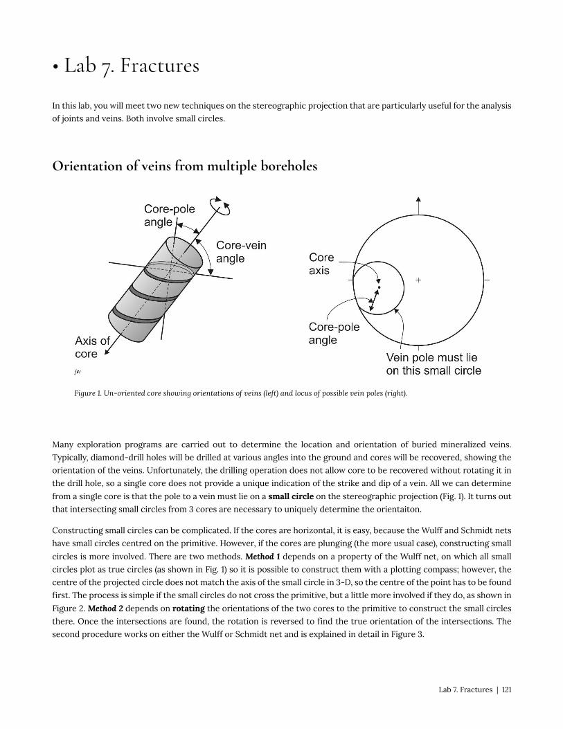
• Lab 7. Fractures

In this lab, you will meet two new techniques on the stereographic projection that are particularly useful for the analysis

of joints and veins. Both involve small circles.

Orientation of veins from multiple boreholes

Figure 1. Un-oriented core showing orientations of veins (left) and locus of possible vein poles (right).

Many exploration programs are carried out to determine the location and orientation of buried mineralized veins.

Typically, diamond-drill holes will be drilled at various angles into the ground and cores will be recovered, showing the

orientation of the veins. Unfortunately, the drilling operation does not allow core to be recovered without rotating it in

the drill hole, so a single core does not provide a unique indication of the strike and dip of a vein. All we can determine

from a single core is that the pole to a vein must lie on a small circle on the stereographic projection (Fig. 1). It turns out

that intersecting small circles from 3 cores are necessary to uniquely determine the orientaiton.

Constructing small circles can be complicated. If the cores are horizontal, it is easy, because the Wulff and Schmidt nets

have small circles centred on the primitive. However, if the cores are plunging (the more usual case), constructing small

circles is more involved. There are two methods. Method 1 depends on a property of the Wulff net, on which all small

circles plot as true circles (as shown in Fig. 1) so it is possible to construct them with a plotting compass; however, the

centre of the projected circle does not match the axis of the small circle in 3-D, so the centre of the point has to be found

first. The process is simple if the small circles do not cross the primitive, but a little more involved if they do, as shown in

Figure 2. Method 2 depends on rotating the orientations of the two cores to the primitive to construct the small circles

there. Once the intersections are found, the rotation is reversed to find the true orientation of the intersections. The

second procedure works on either the Wulff or Schmidt net and is explained in detail in Figure 3.

Lab 7. Fractures | 121

Figure 2. Method 1 for orienting a planar surface intersected by three differently-oriented drill holes.

122 | Lab 7. Fractures

Figure 3. Method 2 for orienting a planar surface using three differently-oriented drill holes.

Lab 7. Fractures | 123

Density plots of poles

Sometimes large numbers of joints are measured in a particular area. Geologists may want to know the mean orientation

of the joints, or to make statements about the variation in their orientation. Normal arithmetic methods for calculating

averages don’t work for orientation data, because orientations are vector quantities. (To understand the problem, try

finding the average of two trends close to north, 359° and 001°. The arithmetic average, 180° or due south, is obviously

nonsense!)

It’s usually more helpful to start with a contoured plot showing the density of poles on a stereographic projection.

Because we are analysing densities of poles, it is important to use an equal-area projection (Schmidt net) for this

process.

Figure 4. Example of a contoured equal area projection (contours show density of data per 1% area of projection).

The first step in any contouring process is to superimpose the data on a grid. For this purpose you can either tape the

projection down onto a piece of graph paper or you can draw a grid directly on the projection. For the example in the

assignment, a grid has been drawn on a plot of poles.

Next, we need to find how many data points lie in each 1% of the net. To do this, a device called a counting circle is

helpful. It can be a piece of paper with a circular hole, or a piece of tracing paper with a circle drawn on it.

In either case, the diameter of the circle must be exactly one tenth of the diameter of the equal-area net; its area will

then be 1% of the net area.

124 | Lab 7. Fractures

Figure 5. Procedure for counting pole density using a counting circle (left) and a peripheral counter (right).

Place the counting circle directly over a grid intersection on the equal area plot. Count the number of poles that fall

within the circle. Write this number on the grid intersection. Repeat with all the intersections in the plot.

For intersections that fall near the edge of the plot, part of the counting circle will fall outside the primitive. The points

that ‘should’ be in this part of the counting circle will appear on the opposite side of the net. We therefore use a second

device, called a peripheral counter, which has two counting circles, their centres spaced apart by the same distance as

the diameter of the net. A slot in the centre of the peripheral counter fits over the thumb tack in the middle of the plot,

so as to keep the counter correctly aligned. When one hole is centred over a grid intersection near the primitive, the

circle on the opposite side contains the extra points that should be counted.

Finally, make a smooth contour map of the results. As in all contouring, make sure that higher numbers all appear on

one side of a contour, and lower numbers on the other. Contours should never branch. In contouring, remember that

contour lines that disappear over the primitive should reappear on the opposite side of the net. Number the contour

lines in percent, meaning “percent of the data occurring in each 1 % of the plot area”.

Assignment

1. A mineral exploration company drilled three diamond drill holes to intersect a vein set in the subsurface. The

angles between the axes of the cores and the veins are shown in the following table.

Drill hole # Trend & plunge of hole Core-vein angle Core-pole angle

1 340-70 NW 40 50

2 080-76 NE 65 25

3 210-68 SW 54 36

Lab 7. Fractures | 125

Calculate the strike and dip of the vein set.

2. You are provided with an equal area projection of 100 poles to conjugate shear fractures in the Cadomin

Formation from the Alberta foothills. To find the maximum densities of points, it is helpful to construct a

contoured plot. A grid has been constructed across the projection to assist with contouring.

a) First, cut out the centre counter and peripheral counting circles precisely. The counting circles have a diameter

exactly 10% of the plot, which means that their area covers 1% of the plot. Use the counting circles to mark

densities at the each grid intersection. Contour the resulting densities on the grid. Remember the principles

of contouring that you used in the first lab: each contour should separate higher from lower values; make the

contours as smooth as possible while honouring the data; contours should never branch. In addition, remember

you are really contouring on the surface of a sphere, and the pattern is symmetrical on the lower and upper

hemispheres. Therefore, if a contour disappears over the primitive, it should reappear on the opposite side of the

projection. When you are done, make a clean copy with selected contours on a separate tracing sheet.

b) Mark estimated centres, or modes, of the two density clusters. These are poles to the typical conjugate shear

planes. From these poles, determine the strike and dip of the two planes, and draw the planes as great circles on

your plot.

The maximum principal stress is predicted to bisect the acute angle between the two planes. The minimum

principal stress bisects the obtuse angle, and the intermediate stress is parallel to their intersection.

c) Mark the principal stresses on your contoured projection and determine the plunge and trend of each.

d) An oil company is interested in flow through extension joints in the Brazeau formation. Predict the orientation

of these joints based on your estimates of the directions of the principal stresses.

Lab 7. Question 2. Plot of poles to 100 shear fractures in Cardium Sandstone, Alberta Foothills.

Lab 7. Question 2. Counting Tool

3. *Look at the geological map of Canmore (east half) which shows numerous faults. Notice the band of dark blue

Palliser Formation in the region north of Exshaw.

a) Without using the cross-section, what is the evidence that the Palliser Formation dips to the SW in this area?

b) Now look at the Palliser Formation on cross-section 1, which extends into the sheet Canmore (west half). Place

two sheets of tracing paper so as to cover the cross-section, and trace only the base of the Palliser Formation

(DPa) and the faults that offset it. For each of the named thrust faults, answer the following questions:

c) Does the fault place older over younger or younger over older strata?

d) Estimate the the dip separation of the base of the Palliser formation. Note – if the fault is curved, you can

approximate the separation with a series of straight-line measurements with a ruler.

e) Estimate the throw and the heave. (These are straight line measurements even if the fault is curved.)

4. *Strictly speaking, you have no evidence for the direction of movement on the faults: – it could be exactly parallel

to the cross-section or there could be a component of strike-slip movement, in and out of the page. However, it is

clear that there has been substantial overall shortening of the rocks in the hanging wall of the lowest, McConnell

Thrust. Estimate this shortening in the line of the cross-section, as follows:

126 | Lab 7. Fractures

a) Measure the total original length l0 of the segments of the base of the Palliser Formation in the cross-section.

b) Measure the present-day distance l between the easternmost outcrop of the base of the Palliser, and the

western edge of the section.

c) Calculate the shortening in kilometres: l0 – l.

d) Calculate the longitudinal strain as a value of stretch: s = l / l0.

e) Calculate the longitudinal strain as a fractional change in length or extension: e = (l – l0) / l

Map. Geology of Canmore (East Half)

Cross-sections. Geology of Canmore (East Half)

Lab 7. Fractures | 127

K. Faults

Introduction

Fractures are known as faults if there has been significant displacement

of one side relative to the other, parallel to the fracture plane. Faults have

had enormous economic impact in the exploration for natural resources.

Faults affect the flow of fluids in the Earth’s crust, and thereby control the

distribution of water, oil and natural gas. Fractured material along a fault

plane may form a porous breccia (pronounced “bretchya”). Fluid passing

through breccia may deposit valuable minerals. Faults are also important

to humans because they generate earthquakes.

An extensive terminology has developed around faults, their geometry,

and movement (kinematics). It is important to distinguish between

descriptive (geometric) terms, which tell us about the orientation of a

fault and the offset of layers on either side, and kinematic terms, which

describe the distance and direction of fault movement.

Faults, fault zones, and shear zones

Figure 1. Fault, fault zone, shear zone.

Strictly speaking, a fault is a single fracture surface. However, many mapped faults turn out to have multiple fault

strands, all roughly parallel, but branching and joining (“anastomosing”) along their strike. This type of fault array is

K. Faults | 129

called a fault zone. The total offset of the fault zone is distributed across the zone. Each fault in the zone offsets the

rocks on either side by a small amount. These add up across the fault zone to a much larger offset.

A related structure is a shear zone. A shear zone is the ductile equivalent of a fault zone – a belt of rock across which

movement has caused a significant amount of offset between the two sides. However, a shear zone is a ductile structure,

typically formed at depth where the deformation of the mineral grains is plastic, not brittle. The movement in a shear

zone is distributed across the zone, rather than being restricted to discrete brittle faults. It is likely that most faults that

deform the upper crust pass at depth into shear zones in the lower crust.

At [pb_glossary id=”779?]map scale[/pb_glossary], faults and shear zones look the same – a line across which older

structures are offset. At outcrop (mesoscopic) or microscopic scale they look rather different.

The orientation of natural faults often varies and they eventually disappear along strike; however, they do tend to have

surfaces that are more planar than other types of geological surfaces, at least over distances of a few kilometres. Faults

can be recognized at a variety of scales from centimetre-scale offsets in an individual outcrop to faults that can be traced

on the ground for tens to hundreds of kilometres such as the San Andreas Fault.

130 | K. Faults

Figure 2. Block diagram of a simple fault offsetting a single surface (dark grey). Below, the same fault is shown as it might appear on a map and in a cross-section parallel to the dip-direction (a dip section). The grey diagram shows a map of the fault plane, known as a fault plane section.

Fault geometry

Strike and dip

A fault is a planar geologic structure. Like any planar

structure, it has an orientation that may be characterized

by strike and dip. For small faults, it may be possible to

walk up to an outcrop and measure the orientation with a

clinometer. Large faults tend to be poorly exposed,

because rocks close to the fault plane are fractured and

broken, and therefore are easily weathered. For large

faults, the orientation may be more easily determined by

drawing structure contours. If the fault is planar, the

strike and dip will be constant, and the structure contours

will be parallel, straight, and equally spaced. If the fault is

curved, then structure contours may show changes in

orientation and spacing.

The blocks of rock on either side of a fault plane are the

walls of the fault. If a fault has a dip (other than 90°) then

one wall overhangs the other. For example, if a fault dips

east, then the east wall must overhang the west wall. The

wall located on the down-dip side of the fault is called the

hanging wall. The wall located to the up-dip side of the

fault is called the footwall.

If these are not clear, think of a geologist standing in a

small cave exactly on a fault plane that dips moderately.

The geologist’s feet will rest naturally on the footwall,

while the hanging wall will overhang the geologist’s head.

If a fault is vertical, it is not possible to characterize a

footwall and a hanging wall. Under those circumstances it

is better to use compass directions to identify the walls:

e.g. “east wall”.

Offset and separation

If a fracture is a fault, there will also be offsets of beds or other older surfaces that are cut. On a map or cross-section,

the points where the trace of a fault cuts the trace of an older surface are called cutoff points (or cut-off points). In three

dimensions, the lines where a fault intersects an older surface are called cutoff lines (Fig. 3). The distance between

the two cutoff lines, for a given surface, is called the separation of the surface. In plan view, as seen on a map of a

horizontal surface, the distance of offset measured parallel to the strike of the fault is called the strike separation. The

strike separation can be sinistral (also known as left-lateral) or it can be dextral (also known as right-lateral). In cross-

section view, parallel to the dip of the fault, the separation is called dip separation. If the beds in the hanging wall are

K. Faults | 131

offset below those in the footwall the separation is normal. If the beds in the hanging wall are offset above those in the

footwall then the separation is reverse. The vertical and horizontal components of dip separation were very important

in old mining operations, and are known as throw and heave respectively.

It’s important to realize that these measurements of separation are geometric. They tell you little about kinematics. In

the diagram below, the arrows on the fault plane show that an infinite number of slip directions is compatible with a

given fault separation.

One feature that may be recognized in the field and is a common result of relatively recent fault activity is the

development of a fault scarp, which is that part of the failure surface exposed by movement of the rock masses. In

studies of recent faults (neotectonics) the fault scarp may give an indication of separation.

However, over time the high-standing block tends to be levelled by erosion. The surface expression of the scarp is

subdued or eliminated and may be of little help in locating ancient faults. Where fault scarps do occur along ancient

faults, the direction of slope tends to be determined by which side has the more erosion-resistant rocks, not by the

sense of separation on the fault. In fact, locating faults in Precambrian terrains may be quite difficult because rocks

affected by faulting tend to be easily eroded. Such faults often occur in low-lying regions occupied by swamps, streams

or heavy vegetation.

Fault kinematics: measuring slip

Slip

The slip is a line that lies in the fault plane; slip represents the distance and direction of movement between the two

blocks of rock on either side of the fault. The slip is a vector – it has a distance and direction. The direction of slip may

be specified by trend and plunge, or by rake within the fault plane. When the rake of the slip is close to the strike of the

fault, the fault is called a strike-slip fault. When the rake is near 90°, close to the dip of the fault, the fault is a dip slip fault.

132 | K. Faults

Figure 4. Slickenlines on a fault surface, Arisaig, Nova Scotia.

Figure 3. Fault plane intersecting a bedding surface, producing cutoff lines in the hanging wall and footwall. Multiple possible slip vectors are compatible with the same geometry.

It is important to understand that slip cannot be determined from the separation of a single offset surface; we need additional information such as slickenlines (scratches or fibres on the fault surface) to give us the direction of the slip.

Figure 3 illustrates the problem: multiple slip vectors would be consistent with

the separations shown by the fault.

Piercing points

If we have a line that is cut and displaced by the fault, we can solve uniquely for

the slip vector. The intersection of a line with a fault plane produces a point,

called a piercing point. If we can locate the piercing points for the blocks on

either side of the fault then we will be able to determine the displacement vector

as shown in Figure 5.

K. Faults | 133

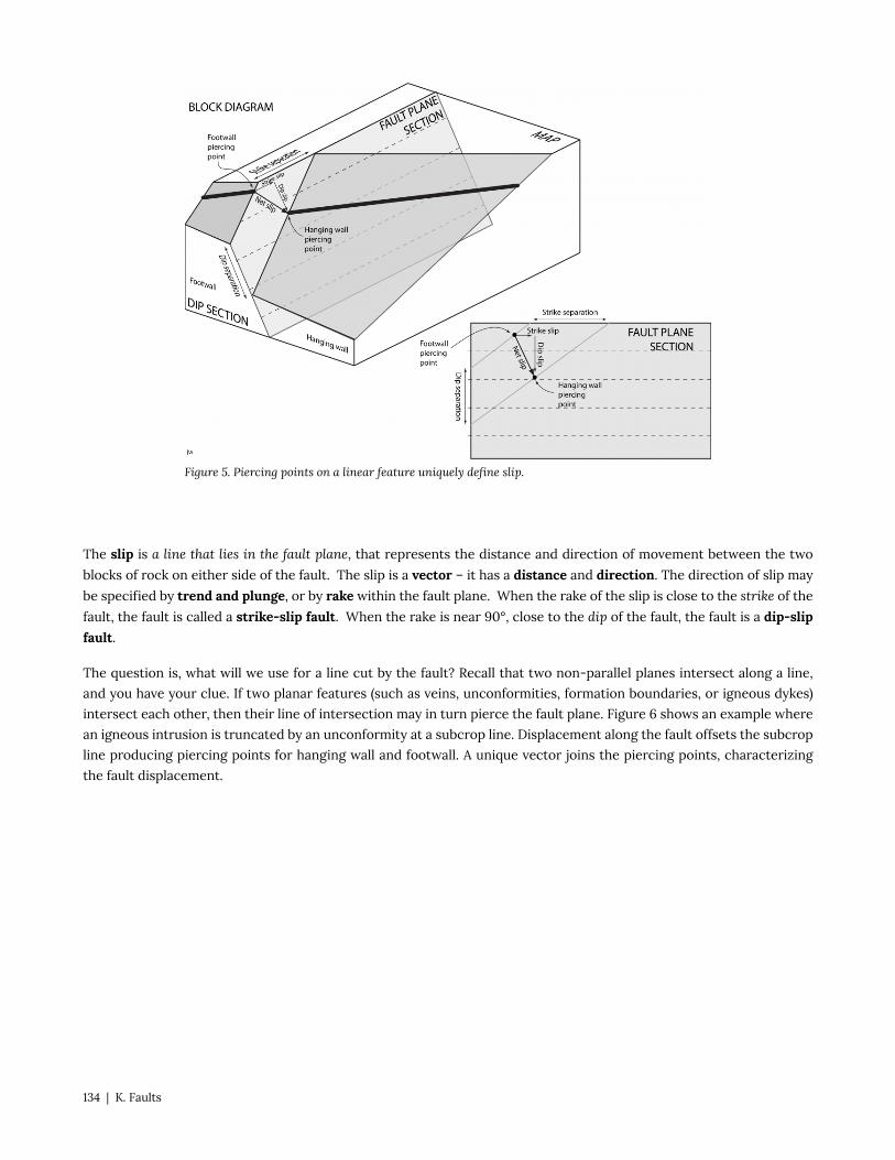
Figure 5. Piercing points on a linear feature uniquely define slip.

The slip is a line that lies in the fault plane, that represents the distance and direction of movement between the two

blocks of rock on either side of the fault. The slip is a vector – it has a distance and direction. The direction of slip may

be specified by trend and plunge, or by rake within the fault plane. When the rake of the slip is close to the strike of the

fault, the fault is called a strike-slip fault. When the rake is near 90°, close to the dip of the fault, the fault is a dip-slip fault.

The question is, what will we use for a line cut by the fault? Recall that two non-parallel planes intersect along a line,

and you have your clue. If two planar features (such as veins, unconformities, formation boundaries, or igneous dykes)

intersect each other, then their line of intersection may in turn pierce the fault plane. Figure 6 shows an example where

an igneous intrusion is truncated by an unconformity at a subcrop line. Displacement along the fault offsets the subcrop

line producing piercing points for hanging wall and footwall. A unique vector joins the piercing points, characterizing

the fault displacement.

134 | K. Faults

Figure 6. Subcrop line defining slip of a fault.

Fold hinges also make excellent piercing points. Figure 7 shows an example.

Figure 7. Fold defining slip of a fault.

K. Faults | 135

Figure 8 shows a second circumstance in which the net slip can be calculated. In this example, striations on the fault

surface (known as slickenlines) allow the direction of slip to be determined. It is then possible to construct artificial

piercing points on cutoff lines at opposite ends of a single slickenline. The amount of slip can be measured between the

constructed piercing points.

Figure 8 Slickenlines defining slip of a fault.

Components of slip

Once the net slip vector is known, it can be broken down into components. The component of slip parallel to the strike

of the fault is the strike slip. The strike slip may be characterized as sinistral (or left-lateral) or dextral (right-lateral). The component parallel to the dip of the fault is called the dip slip. The dip slip may be characterized as normal or

reverse, depending on whether the hanging wall moved up or down relative to the footwall. If the dip slip is much larger

than the strike slip, then the fault is a dip-slip fault; the rake of the slip in the fault plane is close to 90°. If the strike slip

is much greater, then the fault is a strike-slip fault; the rake of the slip is close to zero or 180°. If the dip slip and strike

slip are of comparable magnitudes, then the fault is an oblique-slip fault.

Fault-plane sections

Most calculations involving fault slip are best carried out on a cross-section that lies in the fault plane. Figures 3, 5, 6,

and 7 are each illustrated with a diagram showing a fault-plane cross-section. Most of the significant measurements

of separation and slip can be made directly on the fault-plane cross-section. Of course, in general such a cross-

section will not be vertical. Special techniques are necessary for the construction of non-vertical cross-sections. A plan

view of a dipping geological surface is sometimes called an orthographic projection (because features are projected

136 | K. Faults

perpendicular to the surface onto a plane sheet of paper) and sometimes called a folding line construction (because we

treat the sloping fault plane as if we have folded it around one of its structure contours until it is in the horizontal plane

of a table top.) Typically, we begin by placing a sheet of paper with its edge along one of the structure contours on the

fault plane. This line becomes the folding line. Next, we use a stereographic projection or contours to determine the

rake of various lines on the fault surface and draw them in.

Sometimes it also helps to draw the projected structure contours as horizontal lines on a fault-plane section, to show

elevations above sea level (see fault-plane sections in Figures 3, 5, 6, and 7). The lines are not spaced as they would be

on a vertical cross section. If the contour interval is i and the fault plane has dip d, the spacing of the contours on the

fault plane section will be:

i’ = i / sin(d)

Features of faults in the field

In the description of individual faults, it is generally possible to distinguish a core zone from a surrounding damage zone.

In the core, the rock has been broken up and moved around by fault movement so that the original pieces are separated

from their neighbours. In the core zone it is no longer possible to see how the original pieces for faulted rock were

fitted together.

In the damage zone, the rocks are fractured and may show other deformation features such as folds. However, the

movement is not so great as to obliterate earlier structures, and it is at least possible to see how the pieces of damaged

rock can be fitted back together.

K. Faults | 137

Figure 8. Fault breccia, Guysborough County, Nova Scotia

Figure 9. Microscope thin section of cataclasite. Field of view ~1 cm.

Fault rocks: fault core

Several names are given to fragmented and other rocks of the fault core.

Breccia is a rock composed of typically angular fragments of the walls of the fault

that have been rotated and moved out of their original positions. The fragments

in a fault breccia may be huge, or may range down to about 2 mm. The term

microbreccia may be used for a fine-grained breccia. Although the grain-size

limits for breccia and microbreccia are not precisely standardized, it is reasonable

to use microbreccia for fragments that are 2-4 mm in diameter (by analogy with

the grain size of microconglomerate in sedimentary petrology).

Cataclasite is fragmented material that is sand-size or smaller. Note that neither

breccia nor cataclasite typically has a fabric – the fragments are randomly

oriented.

Gouge is the name given

to clay-rich fault

material, typically

produced from faulting

of fine-grained

sediments. Because clay

can behave in a ductile manner even under near-surface

conditions, gouge can develop some fabric, because the clay

particles become smeared into an orientation parallel to the

fault plane. Gouge is typically very soft in outcrop. In the

subsurface, gouge is very important, as a thick gouge layer may

make a fault plane impermeable to fluids, whereas breccia and

cataclasite are typically permeable.

[Note on mylonite: Mylonite is a name given to fine-grained

rock that has formed through ductile shearing and recrystallization in a shear zone. Mylonite is distinguished from

breccia and cataclasite because it has a strong metamorphic fabric and often shows spectacular crystallographic

preferred orientation – CPO – when viewed under the microscope in thin section. Confusion arises because when

mylonite was first described in the 19th century, it was thought that the fine grain size resulted from brittle fracturing

– the word ‘mylonite’ is derived from a Greek word for milling flour. In the 20th century the study of metals in industrial

processes showed that ductile deformation could lead to the grain-size reduction seen in mylonites]

Pseudotachylite is material that was melted by heating during fault movement. Pseudotachylite is typically dark and

very fine-grained or glassy. It may occur in small dykelets that penetrate the wall rock of the fault. Pseudotachylite

takes its name from an old term for a very fluid igneous lava, tachylite. Pseudo-tachylite looked the same but had a very

different origin.

Deformation adjacent to faults

Riedel shears are small shears that develop in response to stresses in the fault walls during fault propagation and

movement. Synthetic Riedel shears, or R-shears, have an orientation at about 15° to the main fault plane, and display

138 | K. Faults

the same sense of shear as the main fault, as shown in Fig. 10. Less commonly, antithetic Riedel shears, or R'-shears, are also developed, at about 75° to the fault plane. These have a sense of shear opposite to that of the main fault. The

synthetic and antithetic shears form a conjugate set, and therefore can be used to indicate the orientation of the stress

axes when they formed.

Figure 10. Riedel shears associated with a dextral fault.

Fault-bend folds. If a fault is curved, movement of the fault inevitably causes bending of either the hanging wall or

the footwall or both. (If this did not happen, caverns would open up within the Earth as faults moved; lithostatic

pressure prevents this from happening.) Fault-bend folds are particularly common in thrust belts like the Canadian

Rocky Mountains.

Figure 11. Fault-bend folds above thrust fault in siderite bed, Stellarton, Nova Scotia.

Detachment folds. Sometimes, the amount of slip on a fault varies across the fault surface. Some sections have moved

more than others. At the boundary between the sections, deformation in the wall rocks becomes intense, sometimes

leading to the formation of detachment folds.

K. Faults | 139

Figure 12. Detachment fold, Mount Rundle.

Drag folds. Sometimes, a fault will ‘lock’ during its development, and if this happens deformation may be spread through

the wall rocks. If conditions are right, this deformation may be ductile and features in the wall rocks may be bent so

that they become folded. Such folds are called drag folds. Drag folds can closely mimic fault propagation folds (below)

that are formed at the tip of a fault as it develops. Many folds formerly categorized as drag folds are now interpreted as

fault-propagation folds.

Figure 13. Drag fold.

Fault-propagation folds form as faults develop, and combine some of the features of fault-bend and detachment folds.

As a fault develops there will be a fault tip at the point separating slipped rock from rock that has not yet slipped. Fault-

propagation folds form at this fault tip, and shorten one wall of the fault relative to the other. They are also common in

thrust belts like the Rockies.

140 | K. Faults

Figure 14. Fault propagation fold (based on a computer simulation by H. Charlesworth).

Figure 15. Fault propagation fold, Arisaig, Nova Scotia.

K. Faults | 141

Lab 8. Measuring Fault Slip

In Lab 7 you dealt with fault constructions that involved the separation of surfaces, but not with fault slip. This is because

cut-offs for a single plane surface are inadequate to determine the displacement vector, or slip of a fault. In this lab you

will analyse areas where piercing points can be located in both the footwall and hanging wall of a fault, allowing the true

slip to be determined.

Assignment

1.* Map 1 shows a simple map of a level landscape 500 m above sea level, in which a fault offsets a mafic dyke with a

strike separation of 450 m. Slickenlines on the fault trend toward the south and have rake of 060°. Determine the slip

of the fault.

a) *Plot the fault and the dyke as great circles on a stereographic projection. Also plot the slickenline lineation, and

the intersection line, where the fault and dyke intersect. Use a small ‘×’ for the linear data.

b) *Now draw a fault-plane cross-section, viewed from the southwest. This section will show what you would see

if you were able to remove the hanging wall block completely, and look directly at the fault face on the footwall.

The land surface should be a horizontal line at the top of the section. The cutoff-line of the dyke in the footwall

should be shown with its correct rake. Draw a few of the slickenlines, also with their correct rake.

c) *Now mark, using a dashed line, the cutoff of the dyke in the hanging wall (450 m across strike from its position

in the footwall). Draw a line between the two cutoffs, parallel to the slickenline orientation. This is the net

slip. Measure the distance of net slip and determine its trend and plunge from the stereographic projection.

Say whether the dip-slip component is normal or reverse. Say whether the strike-slip component is sinistral or

dextral.

2. Map 2 shows an area in which a thick sequence of conglomerate (circles) unconformably overlies mudstone (white)

and coal (black). The area is cut by a major fault running NE-SW approximately. To the east of the fault the coal is not

exposed, but three boreholes at A, B, and D encountered the coal at depth. Borehole C did not encounter coal. Your

objective is to determine the subsurface structure, so as to show the extent of coal in the subsurface. In addition, you

are to define the slip of the fault, using the subcrop of the coal below the unconformity.

Borehole Elevation of Ground Depth to Unconformity Depth to Coal

A 480 180 280

B 513 213 433

C 650 350 absent

D 580 280 310

a) Fault plane

i) Draw structure contours on the fault surface itself. Extrapolate contours down to sea level (0 m).

ii) Determine the strike and dip of the fault.

b) West of the fault the coal is exposed

Lab 8. Measuring fault slip | 143

i) Identify the unconformity by labelling it on the map.

ii) What is its orientation?

iii) Draw structure contours on the coal seam (assume that the coal seam is thin relative to the scale of the map,

and therefore treat it as a single surface). Terminate the contours where they intersect the fault.

iv) What is the orientation of the coal?

v) Mark the subcrop line on the map where the unconformity surface cuts the coal seam.

c) East of the fault the coal is not visible

i) Identify the unconformity by labelling it on the map.

ii) What is the orientation of the unconformity?

iii) The borehole data allow the elevation of the coal seam to be calculated at three points (A, B & D). Use this

information to construct structure contours on the coal seam.

iv) From your contours, determine the strike and dip of the coal east of the fault.

v) Mark the subcrop line where the unconformity surface cuts the coal seam.

d) Separation: Next, investigate the separation of the surfaces that are cut by the fault.

i) Using intersecting contours, mark and label the cutoff lines where the fault intersects the coal seam in the

footwall and in the hanging wall. Between these two lines is a region where a drillhole would encounter no coal.

ii) Find the difference in elevation between the unconformity in the west and the same unconformity in the east.

This is the vertical separation of the unconformity at the fault – the vertical distance between a surface and

its projected counterpart from the other side of the fault. Because the surface is horizontal, it is also the throw (vertical distance between the hanging wall and footwall cutoffs, measured down the dip of the fault plane).

iii) Find the difference in elevation for the coal seam on either side of the fault (the vertical separation). (Note:

Because the coal seam is gently dipping, its separation measurements – vertical separation, throw, and heave are

all slightly different from the corresponding measurements made on the unconformity, which is horizontal.)

iv) Find the distance measured along the strike of the fault, between equivalent structure contours on the coal

seam on either side of the fault. For example you might find the point where the east side 300 contour hits

the fault plane, and the point where the 300 contour on the west side hits the fault plane. This is the strike separation of the fault. It corresponds to the distance that would appear between the two halves of the coal seam

if the land were eroded down to a horizontal surface.

v) Measure the heave of the fault at the coal seam, the width of the zone (measured perpendicular to the strike

of the fault) between the two cutoff lines.

vi) Superimpose a sheet of tracing paper on the map; on it, shade the area where the coal seam is present below

ground level. (Hint: To do this, the best argument is as follows. Originally the coal was present under the whole

area. Since deposition, coal has been ‘removed’ in three ways. First, some coal was removed by erosion prior

to deposition of the conglomerate, at the unconformity surface; second, coal is missing from the fault heave

between the two cutoff lines; third, more coal has been removed by erosion to the present-day topography. Once

you have removed all these areas, whatever is left is the area underlain by coal.)

144 | Lab 8. Measuring fault slip

e) Fault slip: So far, all the measurements you have made concern the separation of various surfaces. Although they

would be very useful to an exploration project seeking the location of the coal seam, they do not tell us the actual

movement on the fault, the net slip. To determine the net slip, it is necessary to find a unique line which has been

offset. There is an identifiable line that has been severed by the fault. This is the line where the unconformity

intersects the coal seam, the subcrop of the coal seam. This line has been split into two parts by the fault, creating

piercing points on both walls. It can be used to pin down the true slip.

i) Set up a fault-plane cross-section.

• Use a piece of graph paper to make a fault plane cross-section, using the sea-level contour as a folding line.

The trace of the fault on the map is somewhat longer than a normal letter-size sheet of tracing paper, but you

will be able to show all the important intersections on a cross-section 25 cm (6.25 km) long, starting at the

southern boundary of the map. First, find the point where the sea-level (0 m) contour on the fault plane

intersects the south border of the map. Call this point X. Measure 25 cm NE along the contour and mark point

Y. Now take a sheet of graph paper and draw a horizontal line 25 cm long, about 5 cm up from the base of the

paper, and mark the ends X and Y.

• Next calculate the spacing of contours on the fault plane. If the fault has dip d, the contour spacing on the

section will be: i’ = i / sin(d)

ii) Add the footwall and hanging wall intersections.

• Place your graph paper with its top edge along the line XY on the map, and mark the places where the footwall

and hanging wall cutoff lines have known elevation. Project these points to their correct elevations on the

fault-plane section.

• Complete the cross-section by drawing the hanging wall and footwall traces of the unconformity and the coal.

Use solid lines to represent the footwall cutoff and dashed lines to represent the hanging wall cutoffs.

iii) Determine the fault slip:

• Identify the piercing points where the subcrop line intersects the fault, in both the hanging wall and footwall.

Join the two points with a dash-dot line representing the net slip.

• Measure and record the distance of net slip.

• The component of net slip parallel to the fault strike is the strike slip. Draw and label the strike slip on the

fault-plane section, and record the distance of strike slip.

• The component down the dip of the fault is the dip slip. Draw the dip slip, and label it. Record the amount of

dip slip.

• Characterize the fault in words overall, as mainly strike-slip, intermediate (oblique-slip), or dip-slip. Say

whether the strike-slip component is sinistral or dextral. Say whether the dip-slip component is normal or

reverse.

f) Check the results on a stereographic projection

i) Find the rake of the net slip in the fault plane, by measuring it with a protractor on the fault-plane section.

ii) Plot the fault plane, the orientation of the coal, the cutoff lines, and the net slip on a stereographic projection,

and determine the plunge and trend of the net slip.

Answer table for fault measurements, Question 2

Lab 8. Measuring fault slip | 145

Strike and dip of the fault:

Orientation of the unconformity west of the fault:

Orientation of the coal seam west of the fault:

Orientation of the unconformity east of the fault:

Orientation of the coal seam east of the fault:

Vertical separation of the unconformity at the fault:

Vertical separation of the coal seam at the fault:

Strike separation of the coal seam at the fault:

Heave of the fault at the coal seam:

Net slip:

Characterize the fault slip:

Lab 8. Map 1.

Lab 8. Map 2.

146 | Lab 8. Measuring fault slip

Figure 1. Typical relationships between stress and faults based on Anderson’s (1960) analysis of near-surface states of stress.

L. Tectonic Environments of Faulting

Dynamics of faulting

Unlike ductile structures, the formation of fractures can be

simulated experimentally using real rock samples subjected to

stresses in presses. Figure 1 shows the common relationship

between shear fractures and stress. Such fractures are known

as conjugate shear fractures. Conjugate shear fractures provide

one of the few circumstances where structural geologists can

make confident dynamic interpretations based on simple field

evidence.

Anderson’s (1905) theory of faulting starts from some basic facts

about stress, and leads to a classification of tectonic

environments into fault regimes. Anderson noted that the

Earth’s surface is effectively a plane of zero shear stress – at

least as far as structural geologists are concerned. (We can

neglect the relatively tiny shear stresses due to the wind and

the flow of water.) This means that the Earth’s surface closely

approximates a principal plane of stress, and the pole, or

normal, to the Earth’s surface must be one of the principal stresses. Because the Earth’s surface is regionally close to

horizontal, this means that over large areas of the Earth’s

surface, one of the principal stresses is vertical, and the other two

are horizontal.

Note that this argument strictly applies only at the Earth’s

surface. Once we descend to lower levels in the lithosphere, the

principal stresses can, and do, wander away from their vertical

and horizontal orientations.

Based on which principal stress is near-vertical we can classify

environments in the Earth’s upper crust into the following three

categories.

Gravity régime: σ1 vertical: structure dominated by normal

faults.

Thrust régime: σ3 vertical: structure dominated by thrust

faults.

Wrench régime: σ2 vertical: structure dominated by strike-slip

faults.

L. Tectonic environments of faulting | 147

Rifts and extensional zones: normal faults

Occurrence

Several parts of the Earth’s crust are undergoing horizontal extension and crustal thinning at the present day. The best

studied examples are probably the Basin and Range province of the western USA, and the East African Rift valley, which

extends several thousand kilometres through Africa.

We can find ancient examples too. They are particularly well studied underneath passive continental margins,

continental margins which are currently not located at a plate boundary. Passive margins mostly evolved from rift valleys

similar to the East African Rift, as continents stretched and separated in the past. For this reason we find rift structures

buried beneath passive continental margins in many parts of the world. Many of these contain significant petroleum

reservoirs. The Hibernia structure on Canada’s east coast, formed in a rift that developed as the Atlantic opened. Many

of the oilfields in the European North Sea occupy structures related to the Viking-Central Graben, buried beneath

younger sedimentary rocks in the North Sea.

Features of normal faults in rifts

These regions are dominated by normal faults, and in many rifts they have a roughly conjugate geometry: faults dipping

towards and away from each other with dips around 60°, at least near the surface. In many cases faults can be shown to

flatten at depth, giving them listric geometry, though in some cases this is controversial. Some cross-sections of rifts

show faults dipping at a constant angle down to a subhorizontal shear zone in the brittle crust at depth.

148 | L. Tectonic environments of faulting

Figure 2. (a) Listric normal fault. (b) Displacement of hanging wall without folding would lead to a large open space. (c) Hanging wall deforms by fault-bed folding to produce a rollover anticline.

Listric shape has consequences for the geometry of the

walls of faults: one or both walls must distort to maintain

strain compatibility. Typically, the hanging wall distorts

more (because it has a free surface at the top), and

displays a characteristic type of fault-bend fold called a

rollover anticline. Rollover anticlines form important

petroleum traps in many passive continental margins.

Other factors may lead to folding of the wall rocks. It is

common in sedimentary basins for slip to vary across the

surface of a fault, so that slip declines at the edges of a

mapped fault, to a point where there is no slip at all, called

the tip of the fault. How is this accommodated in the wall

rocks? Typically, slip is transferred to another fault, but if

the two faults are not connected, distortion of the wall

rocks may produce a relay ramp linking the two.

Figure 3. Relay ramp between the tips of two normal faults.

L. Tectonic environments of faulting | 149

Arrays of normal faults

Normal faults in rifts do not occur in isolation. Often a cross-section through a rift will show dozens or hundreds of

normal faults. Special terms are given to features of normal fault arrays.

Figure 4. An array of normal faults in a rift.

A horst is a block between two normal faults that dip away from each other, in opposite directions. The rocks in a horst

stand higher than the rocks on either side.

A graben is a block between two normal faults that dip towards each other. The rocks in a graben stand lower than the

rocks on either side.

A half-graben is a tilted block in a rift zone, that is also dropped down relative to the rocks on either side, but it only has

a fault on one side; the other side is typically gently folded.

In many rifts there are a few dominant normal faults with very large offsets. Faults that dip in the same direction are

described as synthetic to the main faults; faults that dip in the opposite direction are antithetic.

Thrust belts

Occurrence

Areas of crustal shortening, dominated by reverse faults, are active at the present day at convergent plate boundaries

(subduction zones), and in areas of continental collision: such as the Himalayas, and Taiwan.

Ancient examples occur in the Rocky Mountains formed in the late Mesozoic and early Cenozoic eras, and the

Appalachian Mountains of eastern North America, formed in the Paleozoic era.

150 | L. Tectonic environments of faulting

In most of these examples folds are intimately associated with thrusts.

In many cases, there is a sedimentary basin, called a foreland basin, adjacent to the thrust belt, and it is thought that

the weight of the thrust belt has depressed the lithosphere as it formed by isostasy. In western Canada, most of the

Cretaceous rocks formed in such a basin, including those that we see in the river valley in Edmonton.

Features of single thrust faults

Geometry: A thrust is any low-angle reverse fault, where low-angle is rather loosely defined. In fact, some thrust faults

are sufficiently curved so that portions would technically be normal faults!

Because of their low angle character, thrusts may look like stratigraphic contacts on maps. There may be closed outlines

of thrusts at hills and valleys.

Figure 5. Features of thrust faults in thrust belts.

• An area of hanging wall entirely surrounded by footwall is called a klippe. • An area of footwall entirely surrounded by hanging wall is called a fenster or tectonic window.

Thrusts are influenced by stratigraphy. In many instances, the dip is steeper in competent rocks like limestone and

sandstone, and shallower in incompetent rocks like shale and evaporites (rock salt, gypsum, anhydrite).

Figure 6. Single thrust fault, showing fault-bend folds developed over ramps and flats.

L. Tectonic environments of faulting | 151

The steeper portions are ramps. They can be recognized on maps and cross-sections because the fault cuts

stratigraphic boundaries at a relatively high angle. On ramps we can find cutoff points. Understanding the kinematics of

a thrust belt often involves matching footwall and hanging wall cutoffs on the same fault. This process is an important

part of checking cross-sections through thrust belts, known as section balancing.

The gentler portions are flats. They can be recognized on maps and cross-sections because the fault surfaces are almost

parallel to the stratigraphic boundaries.

Notice that once a fault has moved, there will be separation between the hanging wall ramps and the footwall ramps,and between the hanging wall flats and the footwall flats. If fault-bend folding occurs, then the hanging wall flats may

acquire steeper dip and the hanging wall ramps may flatten, so this terminology may seem strange! They can still be

recognized by the characteristic cutoff angles of the strata.

A very extensive flat, where there has been a large amount of movement, is called a décollement surface, from a

French word meaning ‘unstick’. If the hanging wall has moved a long way relative to the footwall (tens of kilometres or

more), far enough that the hanging wall rocks were formed in a completely different environment from the footwall,

then the hanging wall is described as an allochthon (from two Greek words, meaning “other place”) and is said to be

allochthonous. The footwall of such a thrust is called the autochthon, and is said to be authochtonous.

For example, in Newfoundland there is a complex of thrust sheets known as the Humber Arm Allochthon that is

composed of Cambrian and Ordovician deep-water sedimentary rocks and ophiolites from the floor of the Iapetus

Ocean. It was thrust on top of sedimentary rocks of more or less the same age range that were formed on a continental

shelf, and therefore represent a very different environment.

Folds associated with thrust faults

Folds may form in association with thrust faults. A wide variety of fold styles are recognized but we will recognize just

three types:

Fault-bend folds: formed where the dip of the fault changes;

Detachment folds: formed where the slip changes, and distortion is accommodated in the hanging wall;

Fault-propagation folds: formed where the dip and the slip change, typically where a fault tip climbs up a ramp during

fault-propagation.

In reality there are many variations on these themes. In particular, there is probably a continuous variation between the

idealized detachment and fault propagation folds.

Arrays of thrust faults

Vergence is a useful concept in dealing with arrays of thrusts. The vergence of a structure is the direction in which

rocks near the surface have moved relative to rocks deeper down. In some thrust arrays, all the thrusts have the same

vergence: that is to say the hanging walls have all been displaced the same way relative to the footwall. Large parts of

the Rocky Mountain thrust belt show eastward vergence, for example. The foreland is the area towards which most of

the thrusts verge: in the Rockies, that is the plains of Alberta. The opposite side of the thrust belt, the side from which

most of the thrust sheets appear to come, is called the hinterland.

152 | L. Tectonic environments of faulting

Figure 7. An array of thrust faults in a thrust belt.

Thrust arrays with similar vergence

Once we start looking at multiple thrusts things can get quite complicated. It is common for multiple listric thrust faults

to branch upward from a single flat. This configuration is called an imbricate fan. The point where one thrust fault

branches from another is called a branch point. In an imbricate fan the branch points mark places where one fault

branches into two as you follow it towards the foreland. This type of branch point is a trailing branch point.

Sometimes imbricate thrust faults merge into flats both upward and downward. Such a configuration is called a duplex. The upper flat is a roof thrust while the lower flat is the floor thrust of the duplex. Like an imbricate fan, the thrusts in

a duplex join downwards at trailing branch points. However, they also join upwards at leading branch points.

Thrusts with opposing vergence: wedges and triangle zones

Sometimes faults in thrust belts have opposing vergence. A pair of opposed thrusts that meet in the subsurface is called

a tectonic wedge. If a third thrust cuts off a triangular section of rock, the wedge is called a triangle zone. The earliest oil

discoveries in the foothills of the Canadian Rockies were found in a triangle zone in the Turner Valley area of southern

Alberta.

Strike-slip zones

Occurrence

Some of the Earth’s best-known faults are strike-slip faults: the San Andreas in California is one of the best-known and

best studied. Other strike-slip faults that have histories of damaging earthquakes include the North Anatolian Fault in

Turkey and the Alpine Fault in New Zealand. Strike-slip faults that are also plate boundaries are called transform faults.

L. Tectonic environments of faulting | 153

Figure 8. Structures associated with strike-slip faults.

Characteristics of strike-slip faults and fault zones

Anderson’s theory of faulting predicts that strike-slip faults should be characteristic of the wrench regime, and that

those faults should be near-vertical. Most major strike-slip faults are found to dip steeply, confirming Anderson’s

prediction. As a result, their traces tend to be very straight lines on geological maps.

The damage zones around strike-slip faults tend to

contain a mixture of structures that we normally

associate either with horizontal shortening (as in thrust

belts) or with horizontal extension (as in rifts). Cross-

sections through strike slip faults tend to be quite

confusing, for this reason. The best way to show what’s

going on in a strike-slip zone is in map view.

In map view, a strike-slip fault zone may be idealized as a

zone of simple shear. For the sake of argument we will

draw a dextral strike-slip zone. (For a sinistral strike-slip

zone everything would be in mirror image.) In a dextral

strike-slip a zone, it’s possible to show that the most rapid

shortening takes place along a line 45° clockwise from the

shear-zone boundary, and the most rapid extension takes

place along a line 45° counter-clockwise from the shear-

zone boundary. For a sinistral strike-slip zone, the

opposite senses of rotation apply.

This idealized pattern of strain rates leads to some

predictions of how structures will form. We predict that

extensional structures like joints, veins, and normal faults,

will form perpendicular to the extension direction, and

shortening structures like folds, thrust faults, and

cleavage planes will develop perpendicular to the shortening direction.

It is also quite common to see subsidiary strike-slip faults, which may include Riedel shears. Dextral synthetic Riedel shears would be predicted at about 15° clockwise from our overall dextral strike-slip zone, while sinistral antithetic Riedel shears would be about 75° clockwise from the overall direction of dextral strike slip. (Reverse everything for a

sinistral zone.)

All these orientations work for fault zones where the overall amount of strain is small. Strike-slip deformation includes

a strong component of rotation, so as deformation continues, all the structures will be rotated. One of the challenges in

interpreting strike-slip motion is that structures may have rotated out of the orientations in which they formed.

Transtension

The above predictions apply to ideal strike-slip motion. However, many of the most interesting structures in strike-slip

zones are formed where there are departures from ideal strike-slip.

154 | L. Tectonic environments of faulting

For example, a combination of strike-slip motion with extension is called transtension. In transtension there is a

component of crustal thinning, along with strike slip, so transtension zones tend to subside and form sedimentary

basins.

One common environment of transtension is at a releasing bend (also known as a releasing stepover) on a strike-slip

fault. If a dextral fault steps to the right, or a sinistral fault steps to the left, the resulting bend is said to be releasing,

and the rocks adjacent to the fault are affected by transtension.

A releasing bend typically develops a localized, parallelogram-shaped subsiding area called a pull-apart basin. In the

Los Angeles area, pull-apart basins associated with the San Andreas system host important natural resources of oil and

natural gas. In Nova Scotia, the Stellarton Basin, also a pull-apart basin on a dextral strike-slip fault system, was a prolific

producer of coal in the 20th century.

In cross-section, pull-apart basins tend to be bounded by families of faults that steepen downwards and merge into a

single fault or shear zone at depth. Individual faults may have normal, strike slip, or oblique slip. This type of fault array

is called a negative flower structure.

Figure 9. Transtension and transpression at releasing and restraining bends on a dextral strike-slip fault.

Transpression

A combination of strike-slip motion with shortening is called transpression. In transpression there is a component

of crustal thickening, along with strike slip, so transpression zones tend to form narrow uplifts, ranges of hills or

mountains.

One common environment of transpression is at a restraining bend (also known as a restraining stepover) on a strike-

slip fault. If a dextral fault steps to the left, or a sinistral fault steps to the right, the resulting bend is said to be

restraining, and the rocks adjacent to the fault are affected by transpression.

A restraining bend typically develops a localized uplift. Parts of the transverse ranges of California, and the Southern

Alps of New Zealand, are associated with transpression at restraining bends along major transform faults.

In cross-section, transpressional ranges tend to be bounded by families of faults that steepen downwards and merge

into a single fault or shear zone at depth. Individual faults may have reverse, strike slip, or oblique slip. This type of fault

array is called a positive flower structure.

Anderson, E. W. 1905. The dynamics of faulting. Transactions of the Edinburgh Geological Society 8, 387-402.

L. Tectonic environments of faulting | 155

• Lab 9. Field Mapping

Introduction

Geologists in the field often need to be able to record the relationships between a set of outcrops so as to collect the

most useful information for geological map construction in the shortest time. Mapping geologists always carry some

kind of base map on which to record their observations. For mapping large areas this might be a topographic map at any

scale between 1:10,000 and 1:50,000. For a small area it may be a sheet of gridded paper on which the geologist records

both geologic and topographic information. Recording information directly on the map while in the field is essential; that

way, cross-cutting relationships such as faults, intrusions, and unconformities can be swiftly and directly portrayed on

the map. Also, you will find out whether you need to collect more evidence for a critical relationship before you leave the field. Modern methods of surveying, particularly the use of the Global Positioning System (GPS), have greatly assisted

map-making at large scale. However, portable GPS units often give errors of 5 m or more in location. Detailed field

relationships may still need to be surveyed using tape-and-compass or pace-and-compass methods.

This exercise will take place at a location where you can practise mapping techniques with a variety of rock types and

structures. Your instructors or teaching assistants will show you the area to be covered. For this exercise you will need

a notebook, a clipboard and a sheet of graph paper, coloured and lead pencils, a compass-clinometer, and your legs!

You will also need to be appropriately dressed and equipped for working outdoors. For all geological fieldwork, it is

important to carry clothing and equipment appropriate to the range of possible conditions you may encounter.

At the University of Alberta, this lab will take place in the Geoscience Garden, a facility that is set up to enable you to practise

mapping techniques with a variety of rock types and structures without leaving campus. Despite its nearby location, you

will still need to be prepared for work outdoors. The weather in Edmonton can be unpredictable. You will probably need

gloves and you may also need a waterproof coat and footwear. Alternatively, if it is sunny you may need sunscreen and a

hat.

Make sure that your compass-clinometer is correctly set for magnetic declination at your location.

The Geological Survey of Canada has a useful declination calculator at:

Magnetic declination calculator: https://geomag.nrcan.gc.ca/calc/mdcal-en.php

For example, in Edmonton AB, Canada, at the beginning of 2020, the declination was 13.8° East

Assignment

The mapping area is large and contains a wide variety of rocks. Your teaching assistants will designate an area for the

mapping exercise.

Lab 9. Field mapping in the Geoscience Garden | 157

Measure your pace

1. * When mapping, it is helpful to be able to estimate short distances by pacing. A tape measure will set up on to

extend 50 m or more through the mapping area. Pace along the tape at least three times to establish the

approximate length of your pace. The most convenient method is to count one for each double pace (one-and-

two-and-three…). In other words count a pace each time your left foot hits the ground. Pace naturally as you

would while walking. Don’t stretch or try to pace extra long steps.

Divide 50 by the average number of paces to get the length of your pace. Round it to a convenient number

like , etc., so that you can approximately convert paces to metres in your head (measurements

approximated to the nearest 1 m are quite good enough).

Also, measure the trend of the tape, and if your basemap has topographic features, locate the tape by pacing from

one end of it to a topographic feature.

2. * Using the scale of your map, draw a line on the graph paper to represent the tape.

Detailed description of first outcrop

3. Choose one outcrop of sedimentary rock and make a detailed description of the rock type(s) as an entry in your

notebook. Give the entry a number. Your description should include grain size, grain shape (if visible), composition

(if you can tell), primary structures (bedding, lamination, cross-lamination, etc.), and secondary structures (folds,

fractures, fabrics). Points to remember in making good field notes:

• Print your notes so that anyone can read them;

• An outcrop may contain more than one type of rock. Make sure that your notes capture the variation from

one lithology to another;

• The degree of detail will depend on the rock-type. For example, in a conglomerate it’s possible to make a very

full description of the clasts, whereas in a mudstone you probably won’t be able to directly observe the grain

shape, sorting, and composition. Don’t claim to observe features you can’t see!

4. Measure the orientation of any layering you see, and identify the type of layering (lamination, bedding, gneissic

banding, etc.

5. Make a diagram of a any evidence that tells you whether the beds are upright or overturned. Points to remember

in making a good field diagram:

• Draw what you actually observe: it’s better to draw a small part of the rock well rather than a large part

showing what you think you should see;

• Your diagram does not have to be artistic. In the field you can take a photo to supplement your diagram, but..

• Your diagram must have labels to indicate what is represented. (You can’t include these on a photo, so even if

you have a camera, making a labelled diagram is still important.)

• Make sure you include an approximate scale bar;

• Include an indication of the orientation of the view, that shows whether you are looking at a plan or a cross-

section.

6. Locate the outcrop on the map; if necessary, draw its outline at approximately the right size and shape. Lightly

158 | Lab 9. Field mapping in the Geoscience Garden

shade the outcrop with a colour. Mark a strike-and-dip symbol in approximately the right orientation beside the

outcrop. Try to place the symbol along strike from the outcrop it describes.

Map observations

7. Locate and describe the other outcrops in the designated area of the garden. Number your notebook entries and

mark the locations on the map. When the rock types are similar, your descriptions can be brief; you need only

describe major differences. However, you should try to measure at least one strike and dip at each outcrop. In the

course of mapping you may encounter folds or faults; measure the orientations of these structures.

8. You will encounter a variety of rock types. Make sure you make a full description of each new rock type in your

notebook. Try to group the rocks you observe into formations. Give each new formation a distinct colour, and build

a legend to the colours on a spare part of the map or in your notes.

Interpreting boundaries

9. As you encounter differences between rock types, try to mark where boundaries might be using dashed lines.

Remember, boundaries between sedimentary rock units tend to be parallel to the strike. After you have decided

where boundaries are, very lightly shade the area where you think each formation is present between the

observable outcrops.

Do not leave the field area until your map shows an interpretation of the geology throughout the are, with clear

interpreted boundaries between units. You can judge the effect of topography much better in the field than in the lab, so complete the map in the field.

Your map must be approved by an instructor or teaching assistant before you leave the field.

After leaving the field

10. On your return to the lab, make a good copy on tracing paper. Mark symbols for the strike and dip of bedding, and

any other structures, this time by measuring them accurately. If you cannot place the symbol exactly on the

outcrop without making the map confusing, offset it slightly to the side, shifting it in the direction of its own strike

or trend.

11. If you encountered a fault or faults, use your observations at a fault to determine the approximate slip, using the

same method you used in Lab 8. If you think the area contains a fold, determine the orientation of the fold axis and axial surface, using the same method you used in Lab 6.

Lab 9. Base map

Lab 9. Field mapping in the Geoscience Garden | 159

• Lab 10. Fold and Thrust Belts

Introduction

The Foothills, Front Ranges and Main Ranges of the Canadian Cordillera are one of the world’s best described fold

and thrust belts, in which sedimentary strata have been shortened by hundreds of kilometres while remaining at low

temperature and showing, at most, low grade metamorphism. Other examples of fold and thrust belts include the

Appalachian Valley and Ridge province the eastern U.S., the Jura Mountains in the Swiss Alps, and the Moine Thrust

zone in NW Scotland. Many of these belts contain substantial reservoirs of oil and natural gas in structural traps, and

therefore considerable effort has gone into understanding their geometry and kinematics.

Because of the relatively low temperatures at which the rocks were deformed, there are strong contrasts between

competent lithologies (typically limestones and sandstones) and incompetent lithologies (typically shales and

evaporites). As a result, faults tend to follow ramp–flat trajectories through the stratigraphy, and most folds are related

to variations in the slip or dip of faults (or both). Also, competent lithologies tend to be translated large distances without

large amounts of internal distortion, except at the hinges of folds. Therefore, fold and thrust belts often show layers

that maintain their original thicknesses; folds of this style are called parallel folds (Fig. 1). These properties are helpful

in the construction of cross-sections, especially in areas where the sheer number of faults and folds make conventional

structure contouring difficult.

Figure 1. Diagrams illustrating idealized characteristics of some common fold styles.

Lab 10. Fold and thrust belts | 161

Techniques for folds in profile

In the first part of this lab, you will explore two techniques for constructing cross-sections through subhorizontal folds

that are useful in preliminary work on thrust-related folds.

Parallel folds are also sometimes called concentric folds, because the curved arcs are parallel, and are centred on

common centres. When a stack of layers exhibits this special geometry, it is possible to make predictions of the

continuation of structures at depth that assist with cross-section construction. We will use the Busk or Arcconstruction

to reconstruct the folds. This construction assumes folds are cylindrical and horizontal folds and the layers have

concentric geometry. The first few steps in this technique are illustrated in Figures 2 and 3. There is also a helpful tutorial

on the worldwide web at the website of Steven Dutch (University of Wisconsin):

• Arc method: https://stevedutch.net/Structge/SL161ArcMethod.htm

Figure 2. Busk construction, step 1.

162 | Lab 10. Fold and thrust belts

Figure 3. Busk construction, step 2.

In some fold and thrust belts, it has been shown that instead of displaying smooth arcs like those postulated in the

Busk construction, folds display straight limbs and angular hinges, like kink folds. This observation leads to the kink construction, in which folds are assumed to have straight limbs and angular hinges. Because beds have the same

thickness on opposite limbs of each fold, the axial surfaces exactly bisect the inter-limb angles. In the kink construction,

rounded fold hinges are approximated by multiple angular folds. Although kink folds depart from parallel geometry at

the hinges, these hinge regions are very narrow; as a result, sometimes the kink and Busk constructions give rather

similar results. First steps in the construction are illustrated in Figures 4 and 5. There is also a helpful tutorial on the

worldwide web at the website of Steven Dutch (University of Wisconsin). Note, however, that the tutorial makes different

assumptions about the locations of fold hinges, compared with the exercise in the assignment, where fold hinges are

explicitly located.

• Kink Method: stevedutch.net/…uctge/SL162KinkMethod.htm

Lab 10. Fold and thrust belts | 163

Figure 5. Kink construction, step 2.

Assignment

1. *Busk construction for parallel folds in profile cross-section

You are provided with a cross-section through an area of horizontal cylindrical folds, with subsurface

information from a single borehole. The scale is 1:10,000, without vertical exaggeration. Dip measurements are

shown at intervals at ground level. Make a cross-section using the Busk, or arc construction.

• To execute the Busk construction, draw a line perpendicular to the dip at each point where the dip was

measured. (Use a protractor and the numerical value of dip from the section.) These lines are called dip

normals. Give them letters A, B, C, etc.

• Find a place where there is stratigraphic information located between two adjacent dip normals e.g. between

A and B. Use a compass with its point placed on the intersection of the bedding normals to extend the

stratigraphic boundaries as far as those normals.

• Continue with the next pair of dip normals, using a compass to extend the boundaries, until the section is

complete. You may assume that the strata beyond the right-hand end of the section dip at a constant 29°.

• The borehole is extended and encounters the base of the Saltmines Gypsum, which is 450 m thick. Add the

base of the Gypsum to the cross section. Notice how the assumption of parallel folding breaks down at depth.

(You may find it easiest to start at both ends of the section, measuring the 450 m of gypsum perpendicular to

bedding in each case, and working toward the ‘difficult’ part in the centre.) Why would you expect the gypsum

to behave differently?

Lab 10. Question 1. Busk Construction

2. *Kink construction for angular folds in profile cross-section

164 | Lab 10. Fold and thrust belts

You are provided a second cross section that shows some additional information in the area of the previous

exercise. A reconnaissance traverse has shown that dip domains are separated by angular folds. The hinges

of these folds are marked ‘H’ with a small x symbol. The new traverse also detected the presence of Brooks

Dolomite at both extreme ends of the section.

• At each fold hinge, construct an axial trace that bisects the bedding dips on either side. the easiest way to do

this is to add the two dips, and divide by 2; this gives the angle from vertical of the bisector. (Be careful if the

dips are in opposite directions; you will need to count one as negative and the other as positive.)

• Then draw the stratigraphic boundaries on either side of the axial trace; you should find that the thickness of

each unit is unchanged as it crosses the fold. Complete the cross-section as before. Make sure you add the

base of the Gypsum as before.

Lab 10. Question 2. Kink Construction

3. Thrust belt cross-section

Map 1 represents a faulted and folded area in a thrust belt. Using the relationships between outcrop shape

and topography, structure contours, and fault-bedding intersection lines (cut-off lines), your objective is to

determine the structure of the area and construct an accurate cross-section along the marked line.

a) Preliminary examination of the map

Look at the outcrop pattern. Both the stratigraphic units and the faults generally have sinuous outcrop patterns

that roughly follow contours in parts of the map, suggesting that in these areas both the faults and the

stratigraphic units mostly have gentle dips. The repetition of stratigraphic units suggest a dipping fault has

caused repetition of stratigraphy. The patterns of faults and outcrops on either side of the main valleys are

rough mirror images of each other, suggesting that the valleys have been eroded through structures that are

now exposed in both valley sides. Any thrust belt map has a lot of surfaces. Identify the major stratigraphic

boundaries and faults with colours as you have done in previous maps. Use red for faults, blues, greens and

browns for stratigraphic surfaces.

b) Cut-off lines

A useful first step is to identify cut-off points, where faults intersect stratigraphic units, and connect them, where

possible, to draw cut-off lines. Remember that for each surface cut by a fault, there will be a hanging wall cut-off

line and a footwall cut-off line. You may notice that corresponding cut-off points have similar elevations on each

side of the main valleys. This suggests that the cut-off lines are almost horizontal. Draw possible cut-off lines on

the map.

c) Structure contours

Now try to draw structure contours on the dipping surfaces. Note that, because we are in a thrust belt, that

surfaces may be repeated, so you may have more than one set of contours on the same surface.

Try to use the minimum number of lines to build the cross-section; however if your map becomes cluttered and

difficult to understand, you may wish to use tracing paper for some of the contour sets. Make sure you record

the position of the corners of the base map on your tracing paper so that it can easily be located, but do not

attempt to trace all the detail from the map onto your tracing paper.

d) Cross-section

Lab 10. Fold and thrust belts | 165

Project all these lines onto the cross section and complete the most reasonable hypothesis you can for the overall

structure on the cross section. Except where you have direct evidence to the contrary, assume a geometry in

which layers maintain constant thickness (either a ‘Busk’ or a ‘kink’ geometry will do, or a freehand compromise

between the two. Your layers should not visibly change thickness across the section.)

Lab 10. Map 1. Fold and thrust belt

166 | Lab 10. Fold and thrust belts

M. Shear Zones

Definition and geometry

Shear zones and faults

Figure 1. Fault, fault zone, shear zone.

Shear zones are zones of intense ductile deformation that are thin relative their lateral extent. Shear zones, like faults,

typically show offsets of older structures, but unlike faults, they lack through-going brittle fractures.

In practice, faults and shear zones are closely related. Many major structures that are faults at the Earth’s surface

probably connect with ductile shear zones at depth, and in the transition it is common to find composite zones that

display combinations of brittle fracture and ductile flow.

At map scale, shear zones can look just like faults, and they display all the same types of geometric relationships (offset,

separation, throw, heave, etc.). We will not repeat those definitions in this section.

At outcrop and microscopic scale, though, ductile shear zones are characterized by planar and linear fabrics. Grain-size

reduction is also common. When it was originally described, the metamorphic rock-type produced by this grain-size

reduction was thought to be a product of brittle grinding (cataclasis) and the rock was named mylonite from a Greek

word for milling flour. We now know better – the fine grain-size is the product of dynamic recrystallization – the

breakdown of the original mineral grains, and growth of new, resulting from the accumulation of defects that result from

extreme plastic deformation.

M. Shear zones | 167

Shear zone kinematics

Where the kinematics of shear zones can be determined, most show a large component of rotational deformation and

many turn out to have undergone progressive simple shear. However, the strain is often heterogeneous, and different

parts of the shear zone show different parts of the strain history, a phenomenon known as strain partitioning.

Figure 2. Incremental and cumulative strain in a homogeneous simple shear zone.

The typical geometry of a shear zone is therefore a band of heterogeneous simple shear, across which previous

structures are offset.

The overall strain inside a zone of ideal simple shear varies. The incremental strain typically shows strain axes at about

45° to the shear zone boundary, but the finite strain shows the effects of rotation: with increasing deformation the shape

of the strain ellipse becomes more and more extreme and the extension direction (X or S1) rotates closer and closer to

the shear zone boundary. Although the extension direction never quite becomes parallel to the shear zone boundary, in

cases of extreme deformation, the difference in direction may be almost imperceptible.

168 | M. Shear zones

Figure 3. Simulation of heterogeneous simple shear applied to a grid of markers. Fabric produced as strain becomes more intense as it curves toward the centre of the shear zone.

Fabrics

Simple sigmoidal foliation patterns

The most basic pattern of foliation in a shear zone is known as sigmoidal oblique foliation. Thisis the fabric that is

produced by the flattening of particles or domains (clasts, mineral grains, etc.)in the protolith (the original rock), when

heterogeneous simple shear takes place.

In the least deformed, marginal parts of the shear zone, the foliation is weak, and oriented ataround 45° to the shear

zone. Towards the centre of the shear zone the foliation intensifies with increasing strain, and it curves so that it is

near-parallel to the overall shear zone. The sense of rotation of the foliation with increasing strain (whether clockwise

or counter-clockwise) shows thesense of shear on the zone.

Lineations

Associated with sigmoidal foliation, the stretched particles of the protolith typically are extended and define a

stretching lineation which gives a streaky appearance to the foliation surface. The orientation of this lineation, when

visible, and its rake in the foliation surface, are important quantities to measure in the field description of a shear zone.

M. Shear zones | 169

Figure 4. C-S fabric.

C-S fabrics

In some shear zones, strain is obviously partitioned such that

zones of intense shear, and grain size reduction, alternate with

zones of less intense strain, where the foliation is more oblique

and the grain size is coarser. This configuration is called C-S foliation (sometimes S-C). The C-planes (where ‘C’ stands for

“cisaillement” in French, meaning shearing) are the surfaces

that are closer to the shear zone boundary and represent the

most deformed bands. The S-planes (for “schistosité”)

represent the less-deformed zones and may be oriented up to

45° from the C-planes and the shear zone boundary. The sense

of rotation from S to C shows the sense of shear on the overall

shear zone.

Shear bands

Figure 5. Diagram of shear-band foliation.

Shear band foliations are geometrically very similar to C-S foliations. They form later in the history of a shear zone,

typically after a strong foliation has been developed throughout. Shear bands take the form of a new set of smaller shear

zones that offset the original foliation. In a dextral shear zone they are clockwise from the original C-planes; in a sinistral

shear zone the orientation is counter-clockwise. Shear bands are also known by the names “extensional crenulation cleavage” and “C-prime (C') foliation“.

Mineral structure of shear zones

It’s possible to learn what goes on in mylonite formation by looking at microscopic thin sections from shear zones. In this

type of work it’s important to collect oriented rock samples. Typically this is done by marking a strike and dip symbol

on a surface of the rock, before the sample is removed with a hammer. Any surface can be marked: a foliation surface or

an arbitrary weathering surface. It’s important to note whether the marked surface is a top surface or an overhanging

170 | M. Shear zones

Figure 6. Undulose extinction and mortar structure, sheared quartz vein, Cape Chignecto, Nova Scotia. In this view, polarizing plates are above and below the microscope stage (cross polars) so that the orientation of quartz crystals can be distinguished in different shades of grey. In this example, dynamic recrystallization has started to occur at grain boundaries, but the grain cores show strongly undulose extinction when viewed between crossed polars. Field of view is approximately 1 cm.

Figure 7. Mylonite, Cape Chignecto, Nova Scotia. In the central part of the slide, the original quartz grains have been reduced to fine-grained mylonite. Field of view is approximately 0.3 cm.

surface. As an additional check it’s useful to flag the right-hand-rule strike direction with an arrow. On a top surface, the

dip direction will be clockwise from the RHR strike direction; on an overhanging surface, looking up, the dip direction

will appear counter-clockwise from the RHR strike direction.

Undulose (undulatory) extinction

On approaching a shear zone, the first thing that is noted

is an increase in the intensity of undulose (undulatory)

extinction when the thin section is viewed between

crossed polars. This is caused by an accumulation of

defects (dislocations) in the crystal lattice.

Mortar structure

With increasing deformation, new tiny crystals appear

along the grain boundaries. These are believed to form

because the accumulation of dislocations makes the

original crystal unstable, so solid-state recrystallization

occurs producing new undeformed crystal lattices. This

process is called dynamic recrystallization.

Eventually the recrystallized material surrounds the original crystals, producing what is known as mortar structure(because it looks like bricks and mortar) or core and mantle structure.

Mylonitic rocks

Rocks which contain significant amounts of dynamically

crystallized fine-grained material are mylonitic.

Mylonitic rocks are classified based on the proportion of

this fine-grained material relative to remaining fragments

of the original rock, known as porphyroclasts. (Don’t

confuse porphyroclasts and porphyroblasts.

Porphyroclasts are large grains in a metamorphic rock

that are left over when the rest of the rock has had its

grain size reduced by dynamic recrystallization.

Porphyroblasts are large grains in a metamorphic rock

that have grown in a fine-grained matrix, typically as a

result of high temperature.)

• Protomylonite

M. Shear zones | 171

Figure 8. Mylonite with porphyroclasts, British Columbia.

Figure 9. Sigma and delta structures.

If the porphyroblasts still make up more than 50% of the rock, then the rock is called a protomylonite.

• Mylonite

True mylonite has from 50% to 10% porphyroclasts.

• Ultramylonite

A rock which is almost entirely dynamically

recrystallized, such that there are less than 10%

porphyroclasts remaining, is an ultramylonite.

Matrix – porphyroclast relations

Because they are less deformed than the surrounding material, porphyroclasts represent sites of strain partitioning, and

sometimes give away the sense of shear in a mylonite. There are two distinctive styles.

• Sigma structure

The foliation sweeps around a sigma porphyroclast in a somewhat rhombic shape, rather like a “small island of

S-plane” in a sea of C-plane. Just like C-S fabric it can therefore indicate sense of shear. It is named after the

shape of the Greek lowercase letter sigma: σσ.

• Delta structure

If the porphyroclast is affected more by the rotation component of deformation, it, together with the foliation in

the adjoining matrix, may be rolled together into a delta porphyroclast named for the Greek letter delta: δδ.

172 | M. Shear zones

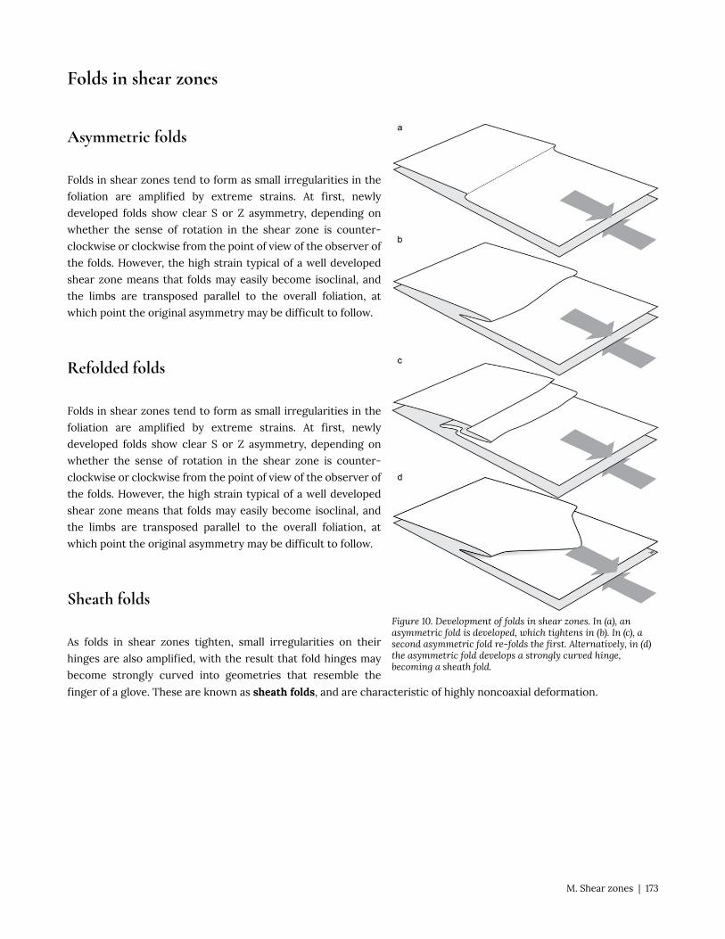
Figure 10. Development of folds in shear zones. In (a), an asymmetric fold is developed, which tightens in (b). In (c), a second asymmetric fold re-folds the first. Alternatively, in (d) the asymmetric fold develops a strongly curved hinge, becoming a sheath fold.

Folds in shear zones

Asymmetric folds

Folds in shear zones tend to form as small irregularities in the

foliation are amplified by extreme strains. At first, newly

developed folds show clear S or Z asymmetry, depending on

whether the sense of rotation in the shear zone is counter-

clockwise or clockwise from the point of view of the observer of

the folds. However, the high strain typical of a well developed

shear zone means that folds may easily become isoclinal, and

the limbs are transposed parallel to the overall foliation, at

which point the original asymmetry may be difficult to follow.

Refolded folds

Folds in shear zones tend to form as small irregularities in the

foliation are amplified by extreme strains. At first, newly

developed folds show clear S or Z asymmetry, depending on

whether the sense of rotation in the shear zone is counter-

clockwise or clockwise from the point of view of the observer of

the folds. However, the high strain typical of a well developed

shear zone means that folds may easily become isoclinal, and

the limbs are transposed parallel to the overall foliation, at

which point the original asymmetry may be difficult to follow.

Sheath folds

As folds in shear zones tighten, small irregularities on their

hinges are also amplified, with the result that fold hinges may

become strongly curved into geometries that resemble the

finger of a glove. These are known as sheath folds, and are characteristic of highly noncoaxial deformation.

M. Shear zones | 173

Figure 11. Sheath fold in mylonitic limestone. Old Man’s Pond, Newfoundland.

174 | M. Shear zones

Meteor Crater, Arizona. By Shane.torgerson – Own work, CC BY 3.0, https://commons.wikimedia.org/w/index.php?curid=12188092. This version has been slightly cropped.

N. Extraterrestrial Impact Structures

Occurrence of impacts

Extra-terrestrial objects impact the Earth sporadically. There is an inverse relationship between size of object and

recurrence interval, although the exact numbers vary depending on whether one considers objects entering the

atmosphere or only those that make it to the surface.

Recurrence intervals for extra-terrestrial impacts of various sizes:

• 10 m diameter: approx. 1 yr

• 50 m diameter: approx. 1000 yr

• 1 km diameter: approx. 500,000 yr

• 5 km diameter: approx. every 10 M yr

• 10 km diameter: 65 Ma event was probably most recent

The object that exploded in the atmosphere over Russia in February 2013 is estimated to have been ~17 m in diameter.

Objects approaching the Earth may vary in speed between about 11 km s‑1 and 72 km s‑1, though smaller objects are

slowed by drag from the atmosphere.

Meteorite impacts produce some of the highest strain rates on Earth. Typical values of strain rate in the first few

microseconds of an impact may be of the order of 108 s‑1. (Contrast the strain rates during an earthquake, typically

0.1 to 10 s-1. By comparison, time-averaged strain rates in orogens due to plate movement are typically 10‑15 to 10‑12 per

second.)

One of the most obvious results of an impact is a roughly circular depression called a crater. Major craters have been

described from many parts of the Earth. The three largest confirmed examples are:

1. Vredefort Crater in South Africa, diameter ~300 km, formed at 2020 Ma, and now deeply eroded;

2. Sudbury Basin, 250 km diameter, formed at 1849 Ma and subsequently deformed;

N. Extraterrestrial Impact Structures | 175

3. Chixulub crater, 180 km diameter, 65 Ma.

Impact craters

Larger impacts form craters, which have two types of geometry (Fig. 1).

Figure 1. Simple and complex craters.

Simple craters

Simple craters are up to about 4.5 km in diameter. They tend to have simple bowl shapes with a raised rim. (On the

moon, where gravity is less, simple craters are up to 15 km diameter.)

Complex craters

Larger craters show complex geometry. The most distinctive feature of complex craters is a central uplift. The inside

of the rim of a complex crater typically shows a series of internal terraces, and the outside of the rim may also

have concentric ridges and valleys. Between the central uplift and the terraces, the floor of a complex crater is often

somewhat flat. These differences may be explained by considering the processes of crater formation, and particularly

the “modification stage” (see below).

176 | N. Extraterrestrial Impact Structures

Figure 2. Three stages of crater development.

Impact processes

Contact and compression

The first stage in the development of an impact crater is

the contact and compression stage, beginning when the

object first touches the surface. In this stage, the

impacting object and the underlying rock are subject to

extremely high strain rates of 108 per second or higher.

These strain rates may produce enormous stresses above

1 TPa (1012 Pa), and very high temperatures, sufficient to

melt or even vaporize large parts of the impacting body

and the rocks in front of it. Rock that remains solid is

compressed in a shock wave that initially propagates at a

speed comparable to that of the incoming body, typically

much faster than normal seismic waves.

As the shock wave passes, rock is highly compressed,

which depresses the Earth’s surface, starting the process

of crater formation. Behind the compressional shock

wave, there is a wave of expansion, where the release of

elastic energy produces very high temperatures, that

melt or vaporize the expanding rock material.

Contact and compression lasts only a few tenths of a

second even for a very large impact.

Eventually the speed of the advancing shockwave slows

down to seismic velocities (3-7 km s‑1) and continues to

propagate through the Earth as a seismic wave, during the

next stage.

Excavation stage

Initially the compressional wave moves rock downward and outward but as the wave expands material is pushed

upwards at the edges of the expanding crater, creating a raised rim. In addition, as the decompression wave passes,

material that was formerly compressed downwards expands upward, and its momentum causes it to be thrown up into

the atmosphere. These processes result in the excavation of material (ejecta), into the air and onto the surrounding

surface. The resulting depression is known as the transient crater.

The maximum size of the transient crater marks the end of the excavation phase. The excavation stage lasts several

minutes in a large crater.

N. Extraterrestrial Impact Structures | 177

Figure 3. Shatter cones, Charlevoix, Quebec.

Figure 4. Shatter cones, Sudbury, Ontario.

Modification stage

The end of the excavation is followed by crater modification. For small craters the modification process is relatively

simple. The floor of the deep transient crater rebounds as the rock decompresses, to produce a shallower, bowl-shaped

depression.

In larger impacts, the process is more complex. Rebound of material that has been compressed vertically downward

is more complete and produces a central uplift. Surrounding it is a region where rebound takes material upwards and

outwards, contributing to the rim. In addition, the rims of these larger craters tend to be unstable, and during the

modification stage, large normal faults form, allowing pieces of the rim to subside as terraces.

Ejecta tend to fall back into the crater, and material may remain molten for long enough to pond on the crater floor.

Large complex craters tend to have flat floors between the central uplift and the terraced rim.

Rock products of impact

There are a number of products of impacts that can be recognized in the ancient record.

Shatter cones

Shatter cones are conical joint surfaces that are typically decorated with plumose markings. Poles to the surfaces of the

cones typically fall on small circles when plotted on a stereographic projection. The axes of the cones point toward the

point of impact and can help to locate this point if their orientations are carefully measured.

178 | N. Extraterrestrial Impact Structures

Figure 5. Sill of impact breccia, Charlevoix, Quebec.

Figure 6. Impact melt (above) intruding granitoid rock (below), Sudbury, Ontario.

Impact breccia and suevite

In areas of greater compression, and therefore greater

subsequent expansion, impact breccia is produced. Impact

breccia may have open spaces between the fragments (which

may be filled by later vein minerals if hydrothermal fluids flow

through), or the spaces may be filled by melt or by a matrix of

small fragments. A fine-grained rock with a breccia texture,

consisting of a mixture of rock fragments, glass, and melt, is

known as suevite.

Impact melt: pseudotachylite

Substantial melting may occur behind the initial shockwave,

producing pseudotachylite, similar to the pseudotachylites

produced by frictional melting along certain faults. However,

much larger volumes of pseudotachylite may be found in impact

structures than are common along faults.

Pseudotachylites have a much wider range of compositions

than those of normal igneous rocks, because they are produced

by more or less complete melting of their parent rocks, rather

than the progressive and partial melting in most igneous

processes.

In the Sudbury structure a thick layer of impact melt underwent

fractional crystallization to yield a thick ore body of massive

sulphide.

New minerals

The very high pressures encountered in the contact and compression stage may cause new, high pressure minerals to

form. The most notable are two high-pressure polymorphs of silica SiO2. Coesite is a monoclinic form of silica in which

the silica tetrahedra are linked in a manner similar to feldspars. It requires pressures above 2 GPa to form. Stishovite is

a very dense phase in which the silicon is in octahedral coordination, surrounded by six oxygen atoms in a tetragonal

structure. Stishovite requires pressures above 8 GPa.

Diaplectic glass

Mineral grains that are subject to extreme and rapid compression may lose their mineral structure, as bonds between

the atoms are broken. On decompression, depending on the temperature, the atoms may be unable to diffuse back

N. Extraterrestrial Impact Structures | 179

into a crystal lattice, with the result that they appear isotropic in thin section, like volcanic glass. However, unlike true

pseudotachylite, this glassy material may still display the outlines and compositions of the original crystals, showing that

it was never truly molten. This material is known as diaplectic glass.

180 | N. Extraterrestrial Impact Structures

Glossary of terms

Acicular

Needle shaped (of mineral grains)

Acive continental margin

A transition or boundary between continental and oceanic lithosphere that coincides with a plate boundary (ridge,

trench or transform fault).

Allochthon

A body of rock that has been moved from its original position, usually in the hanging wall of a thrust fault

Allochthonous

Moved from its original position, usually in the hanging wall of a thrust fault

Angular unconformity

An unconformity characterised by an angular discordance (a difference of strike or dip or both) between older strata

below and younger strata above.

Anticline

A fold in which the younging direction is away from the inside of the fold.

Antiform

A fold where the limbs dip away from the hinge so that the fold closes upward.

Antitaxial vein

A vein filled with mineral fibres, in which the fibres have grown outwards, toward the walls.

Antithetic Riedel shears (R' shears)

Subsidiary fractures that form at about 75° to a fault, with sense of displacement opposite to that of the fault.

Apparent dip

The apparent dip of a surface is its dip measured on a cross-section that is not perpendicular to the strike of the

surface. Apparent dip is always less than true dip.

Arc construction

Busk construction

Attitude

Orientation

Glossary | 181

Autochthon (autochthonous)

A body of rock that has not been moved from its original position, usually in the footwall of a thrust fault

Axial planar foliation

Planar fabric that is approximately parallel to the axial surface of a fold.

Axial surface (hinge surface)

Imaginary surface that passes through all the hinge lines of a fold

Azimuth

A bearing measured clockwise from north from 0 - 360°.

Bar

A force concentration of one million dynes per square centimetre, or 100,000 Pa

Bathymetric contour

Contours that show the depth of the sea floor below sea level .

Bearing

A direction relative to north.

Beds

Sedimentary layers thicker than 1 cm.

Bioturbation structures (trace fossils)

Structures produced by organisms that have disturbed sediment.

Boudin

A structure formed by a layer that has separated into pieces, typically as a result of extension.

Boudinage (pinch-and-swell structure)

The process of formation of boudins.

Branch point

A point where one fault meets and joins another.

Breccia

A rock composed of typically angular fragments, typically from a fault. (The term breccia is also sometimes used in

sedimentary geology for an angular conglomerate.)

Brittle fracture (brittle failure)

Non-recoverable deformation characterized by loss of strength across a surface.

182 | Glossary

Busk construction

A construction for folds in profile view in which the traces of surfaces are assumed to be concentric arcs of circles.

Also known as the arc construction.

C-plane

A surface within a shear zone that is characteristically parallel to the zone boundaries and which shows the most

intense deformation; from the French word "cisaillement" meaning shearing.

C-prime (C') foliation

Shear bands that form later in a history of a shear zone after a strong foliation has been developed throughout.

They are typically oriented oblique to the shear zone boundaries, with the same sense of rotation (clockwise or

counterclockwise) as the overall shear zone.

C-S foliation

Foliation in a shear zone characterized by intensely strained zones roughly parallel to the shear zone (C planes) and

less strained zones where the foliation is oblique (S-planes).

Cataclasite

Fragmented material in a fault zone that is sand-sized or smaller.

Chill zone

Typically finer-grained material found near the edge of an igneous intrusion, typically formed by rapid coolling

Chocolate tablet structure

Boudins that are roughly equant in plan view, produced by extension of a layer in all directions

Cleavage refraction

A change in the orientation of cleavage caused by differences in the mechanical properties of layers. Cleavage

typically bends so that it is more perpendicular to competent layers, and more parallel to incompetent layers.

Clinometer (inclinometer)

A device that measures inclinations.

Coaxial deformation

Deformation in which the strain axes remain fixed to the rock material throughout deformation

Coesite

A monoclinic form of silica in which the silica tetrahedra are linked in a manner similar to feldspars. It requires

pressures above 2 GPa to form.

Columnar joints

Joints that separate elongated bodies of rock that are typically polygonal (roughly hexagonal) in cross-section. These

typically form perpendicular to the base and top of an igneous flow or sill.

Glossary | 183

Compaction

Volume loss due to the expulsion of water as rocks are buried.

Compass

A tool which uses the Earth's magnetic field to measure directions parallel to the Earth's surface.

Competence

A general term for resistance to stress.

Complex crater

A crater that show a central uplift and a terraced outer wall.

Compromise boundaries

Approximately planar boundaries produced when mineral grains grow against one another. Compromise boundaries

are not controlled by the crystal structure of either mineral grain.

Concentric joints

Joints parallel to the surfaces of an intrusion.

Conjugate shear fractures

Fractures formed when when rocks fail simultaneously along two families of planes approximately 60° apart in

orientation.

Contour

A curving line on a map that separates higher values of some quantity from lower values.

Contour interval .

The numerical difference in value between contours on a map

Contour spacing

The horizontal distance between contours recorded on a map.

Convolute lamination

A soft-sediment deformation structure in which laminae are deformed into complex chaotic folds.

Core zone

The central part of a fault, in which brittle deformation has destroyed the continuity of older structures.

Crater

A roughly circular depression formed by a meteorite impact or volcanic activity.

Crenulation cleavage

Planar fabric represented by closely spaced fold axial surfaces. Almost always a second or later generation of fabric.

184 | Glossary

Crenulation lineation

Linear fabric represented by closely spaced fold hinges.

Crest point

The highest point on the cross-section of an antiform.

Crest surface

A surface containing multiple fold crest lines.

Cross bedding

Cross stratification caused by dunes.

Cross lamination

Cross stratification produced by ripples.

Cross stratification

A configuration of laminae produced by migration of bedforms during sedimentation, in which laminae are oriented

at an angle to the depositional horizontal.

Culmination point

The highest point on the crest line of a fold.

Cutoff line

The line where a fault intersects an older surface.

Cutoff point

The point on a cross-section where the trace of a fault cuts the trace of an older surface.

Cylindrical fold

A fold with a well defined axis that is everywhere parallel to the folded surface. Parallel cross-sections cut in

multiple positions through the fold appear identical to each other.

Damage zone

The outer part of a fault, in which remnants of pre-existing structures can still be traced.

Décollement

A very extensive flat in on a thrust fault, where there has been a large amount of movement.

Deformation

The movements of parts of the Earth's crust relative to each other.

Glossary | 185

Delta pyroclast

A prophyroclast around which foliation curves in a tightly curved shape, formed as the porphyroclast and adjacent

foliated rock are rotated in a shear zone.

Depression point

The lowest point on the trough line of a synform.

Descriptive (geometric) analysis

Analysis comprising records of the positions, orientations, sizes, and shapes of structures that exist in the Earth's

crust at the present day.

Detachment fold

A fold produced when wall rocks accommodate variations in slip between different parts of a fault.

Deviatoric stress

The state of stress obtained when the mean stress is subtracted from each of the principal stresses. The deviatoric

stress is the part of the stress system that acts to change shape.

Dextral

Right-lateral movement: relative to an observer looking toward a fault or shear zone, the far side appears to have

moved right.

diaplectic glass

Glass generated by the action of a shockwave on common minerals.

Differential stress

The difference between the largest and smallest principal stress.

Differentiated crenulation cleavage

Crenulation cleavage combined with pressure solution cleavage, producing a foliation that is characterized both by

folds and by parallel domains of different composition.

dike

Dyke (U.S. spelling)

Dilation

Change in size (area or volume)

Dip

The value of the inclination of a plane. Represents the inclination of steepest line that can be drawn on the plane.

Dip direction

The azimuth of the steepest inclined line that can be drawn on the plane.

186 | Glossary

Dip separation

The distance along a fault, measured in the direction of fault dip, between two cutoff lines of the same severed

surface.

Dip-slip fault

A fault in which the component of slip parallel to the fault dip exceeds that parallel to the fault strike.

Disconformity

An unconformity between strata of different ages but identical orientation.

Discordance

A difference of orientation between planes: difference of strike or dip or both.

Disharmonic fold

A fold where the hinges and limbs do not match with those in adjacent layers..

Dislocations

A linear defect in the structure of a crystal where the atoms of the crystal structure are out of alignment.

Distortion

Change in shape

Domain

A region within a rock that has a distinctive composition or texture.

Drag fold

A fold adjacent to a fault in which layers are bent in the direction of movement of the opposite wall. Most 'drag' folds

probably form during fault propagation and not by 'drag' after the fault has formed.

Ductile

Flow of material in the solid state, typically without fracture.

Duplex

A structure in which imbricate inclined thrust faults merge into flat faults both upward and downward.

Dyke

A minor intrusion where magma has filled a crack that is discordant to layers in the surrounding rocks. (Spelled

'Dike' in the U.S.A.)

Dynamic analysis

Structural methods that involve the determination of force, stress, strength, or energy involved in deformation.

Glossary | 187

Dynamic recrystallisation

Breakdown of original mineral grains and growth of new mineral grains as a result of extreme ductile deformation.

Earthquake

Rapid relative motion of parts of the solid Earth due to brittle failure on a fault.

Effective stress

Overall stress minus the fluid pressure.

Elastic

A stress-strain relationship in which stress and strain are proportional, and the strain is recoverable.

En echelon

An arrangement of linear or planar structures where each structure offset from adjacent structures in a consistent

sense that is oblique to the structures themselves. (Literally: as a squadron of cavalry.)

Endocontact

The region within an intrusion where it is affected by contact with the host rock.

Enveloping surface

A surface tangent to multiple folds in a layer.

Equal angle projection

A spherical projection in which angles are preserved. Also known as a sterographic projection. Great and small

circles project as circular arcs. Constructed using a Wulff net.

Equal area projection

A spherical projection in which area is preserved.Great and small circles project as complex, non-circular arcs.

Constructed using a Schmidt net.

Exocontact

The region in the host rock (country rock) affected by contact with an intrusion.

Extension

A measure of longitudinal strain equal to the fractional change in length.

Extension fracture

A fracture where rock masses on either side of a fracture have moved apart slightly, without significant movement

parallel to the fracture.

Extrapolation

The process of estimating values outside the range of a data set.

188 | Glossary

Fabric

Any penetrative structure that gives a rock different properties in one direction relative to another.

Fabric element

Features within a rock that are aligned to give the rock a fabric.

Facing direction

Direction of younging of strata in a fold axial surface.

Fault

A fracture showing significant displacement of one wall relative to the other, parallel to the fracture plane.

Fault bend fold

A fold produced by movement of a curved fault, in which movement of the fault caused bending of the hanging wall,

footwall, or both.

Fault cutoff

Intersection line between a fault plane and an older planar rock unit.

Fault propagation fold

A fold that forms at the propagating tip of a fault, marking a region where there are rapid changes in both the dip

and the slip of the fault.

Fault regime

A tectonic environment in the Earth's upper crust characterized by the orientation of the principal stresses.

Fault scarp

A steep topographic slope marking a fault, where one wall of the fault forms higher ground than the other.

Fault tip

The linear boundary at the edge of a fault surface, separating faulted from unfaulted rock.

fault zone

A set of sub-parallel faults that may branch and joint along strike or down dip.

Fenster (tectonic window)

An area of footwall on a geologic map that is entirely surrounded by hanging wall.

Fibrous vein fill

Mineral grains within a vein that are strongly elongated, typically tracking the direction of movement as the fracture

opened.

Glossary | 189

Finite deformation

The total deformation that a part of the Earth has undergone, between its original configuration and the present-

day state.

Finite strain

The total strain that a part of the Earth has undergone, between its original configuration and the present-day state.

Fissility

The property of splitting easily parallel to a plane, usually the result of sedimentary compaction.

Flame structure

A narrow, pointed soft-sediment deformation structure consisting of mud forced up into overlying sand.

Flat

In fault terminology, a region where a fault is parallel to layers in the wall rocks.

Flattening foliation

A foliation defined by tabular domains, produced by shortening.

Floor thrust

The lower flat of a thrust duplex structure.

Fluidise (Fluidize)

A process whereby previously stable sediment is behaves as a fluid when upward-flowing water passes through it

from below.

Flute

A scoop-like depression in mud that becomes less distinct in a down-current direction.

Flute cast (Flute mold)

A sedimentary structure formed when a flute is filled by sand and preserved in relief on the base of a sandstone bed.

Fold axis

The orientation of a line that is everywhere parallel to a folded surface. The fold axis is the direction of the hinge,

crest, trough, and inflection lines.

Fold hinge

A line of maximum (tightest) curvature on a folded surface.

Fold interference pattern

A pattern formed by layers that have been folded twice during their deformation history.

190 | Glossary

Folding line construction

A construction in which differently dipping surfaces are rotated about their line of intersection in order to represent

them on a plane sheet of paper.

Foliation

Planar fabric

Footwall

The body of rock directly below a fracture.

Foreland basin

A sedimentary basin that forms adjacent to an orogen, and which deepens toward the orogen, typically formed by

bending of the lithosphere in response to the weight of the growing orogen.

Formation

The primary unit of mapping in stratified rock; must be mappable, defined by lithological characteristics, have a

type section, and be named for a place or geographical feature.

Fracture

A surface produced by brittle failure at some point in the history of a rock.

Fracture tip

The linear boundary at the edge of a fracture surface, separating fractured from unfractured rock.

Geologic map

A map showing the extent of, and boundaries between, different units of rock.

Geological boundary

A surface in 3D space, or a line on a 2D map, where one type of rock contacts another.

Glacial striae

Lineation on the Earth's surface formed by abrasion during flow of ice, which reveals the direction of ice movement.

Gneissic banding

Foliation characterised by layered domains of different composition, and the parallel preferred orientation of

minerals, typicall of high-grade metamorphic rocks.

Gouge

Clay-rich fault material, typically produced by faulting of fine-grained sedimentary rocks.

Graben

A block between two normal faults that dip towards each other. The rocks in a graben are offset downward relative

to the rocks on either side.

Glossary | 191

Graded bed

A bed, usually with a sharp base, in which grain-size becomes finer toward the top.

Gravity regime

A state of stress in which the maximum principal stress is vertical. Normal faults are common.

Great circle

A circular line that divides a sphere into two precisely equal parts.

Groove

A sedimentary structure formed when an object is dragged by a current across a sediment surface.

Groove cast (Groove mold)

A sedimentary structure formed when a groove is filled by sand and preserved as a mold on the base a bed.

Group

A lithostratigraphic unit consisting of several formations.

Hackles

Feather-like striae radiating from a central point or line on a fracture. Part of plume structure.

Half-graben

A tilted block bounded by a normal fault on one side, along which the block is offset downward.

Hanging wall

The body of rock immediately above a fracture.

Harmonic folds

Folds in which each layer is folded in step with the adjacent layers, so that hinge points can be matched between

layers

Heave

The horizontal component of dip separation.

Heterogeneous strain

Strain that is not the same everywhere within a rock. Straight lines may become bent and parallel lines may becomeg

non-parallel.

Hinge

A line or point of maximum (tightest) curvature on a folded surface.

Hinterland

The region adjacent to a thrust belt away from which the thrust sheets appear to have moved.

192 | Glossary

Homogeneous strain

Strain that is the same everywhere within a rock. Straight lines remains straight, parallel lines remain parallel.

Horst

A block between two normal faults that dip away from each other. The rocks in a graben are offset upward relative

to the rocks on either side.

Ideal plastic deformation

A ductile behaviour in which a material shows no deformation a certain stress (yield stress) is reached, and then

deforms rapidly so as to prevent the stress from rising futher.

Imbricate fan

A configuration of multiple listric faults that branch upward from a single flat.

Impact breccia

Breccia resulting from a meteorite striking the Earth.

Inclination

An angle of slope measured downward relative to horizontal.

Incremental strain

The strain that occurred during a small interval in the history of deformation.

Infinitesimal strain

The strain that was occurring a single instant during the history of deformation. (The limit of incremental

deformation as the time interval tends to zero.)

Inflection line

A line on a folded surface where the curvature is zero, typically marking a change from convex-up to convex-down,

or from antiform to synform.

Inflection surface

A surface containing multiple inflection lines.

Inlier

A region on a geologuc map where older strata are surrounded by younger strata.

Interpolation

The process of estimating intermediate values between the points in a sparse set of data.

Intersection lineation

A lineation defined by the intersection of two differently-oriented foliations.

Glossary | 193

Invariant feature

A feature that is independent of fold orientation.

Inverse grading

Grain-size variation within a bed in which coarser grains are concentrated at the top.

Isobar

A contour line separating higher pressures from lower; a line joining points of equal pressure.

Isopach

A contour line based on the thickness of a stratified rock unit, separating a thicker from a thiner part of a layer; a

line joining points of equal thickness.

Joint

A fracture where the movement parallel to the failure surface is minimal.

Joint set

Many joints in approximately the same orientation.

Joint system

A combination of joint sets, cross-cutting each other in a regular way.

Kinematics

The study of how parts of the Earth moved over geologic time. Include changes in position, orientation, size, and

shape that occurred between the formation of the rocks and their present day configuration.

Kink construction

A construction for folds in profile view, in which fold limbs are assumed to be perfectly planar, parallel surfaces, and

hinges are perfectly angular

Klippe

A region on a geologic map where the hanging wall of a fault is completely surrounded by footwall.

Lamina (laminae)

A layer thinner than 1 cm; plural "laminae".

Layers

Domains that are very extensive and parallel-sided.

Lineation

Linear fabric; fabric defined by elements that are parallel to a line in space.

194 | Glossary

Liquidize, liquidise

A process whereby previously deposited sediment behaves as a liquid, when the sand grains become separated by

fluid

Listric

Describes a fault with dip that decreases with depth.

Lithosphere

The rigid outer part of the Earth that is divided into plates. Comprises the crust and the uppermost part of the

mantle.

Lithostatic stress

A state of stress in which all principal stresses are equal, due to the weight of overlying rock.

Lithostratigraphic unit

A named rock layer recognized on the base of its lithological characteristics.

Load structure (load cast)

A soft-sediment deformation structure caracterized by rounded bulges, typically on the base of a sandstone bed.

LS tectonites

Rocks with a strong tectonic lineation that lies in the plane of a strong tectonic foliation.

Macroscopic (map-scale) structures

Structures that are too big to see in one view. Must be mapped, or imaged from an aircraft or satellite.

Magnetic contour

A contour line based on characteristics of the Earth's magnetic field; a line that separates stronger magnetic fields

from weaker.

Magnetic declination

The azimuth of the Earth's magnetic field.

Map-scale (macroscopic) structures

Structures that are too big to see in one view. Must be mapped, or imaged from an aircraft or satellite.

Mapping

The process of recording and interpreting data on a two-dimensional plan view such as a topographic base map.

Mean stress

The average of the three principal stresses.

Glossary | 195

Member

A smaller mappable unit recognized within a formation.

Mesoscopic (outcrop-scale) structure

Structures visible in one view at the Earth's surface without optical assistance.

Metamorphic aureole

Baked zone around an intrusion that is often recognizable from changes in texture or mineralogy.

Microbreccia

Fine-grained breccia; breccia with particles 2-4 mm in diameter.

Microscopic structure

Structure that requires optical assistance to be visible.

Mineral lineation

Linear fabric defined by parallel alignment of acicular mineral grains; linear equivalent of slaty cleavage and

schistosity.

Mortar structure

Microscopic structure characterized by rims of fine-grained recrystallised material surrounding remnants of

original crystals.

Mudcracks

Thin fractures on the surface of beds that thin downward, form by shrinkage of mud as it dries.

Mylonite

Fine-grained rock formed through ductile shearing and dynamic recrystallisation in a shear zone.

Mylonitic lineation

Stretching lineation formed during extreme ductile shearing.

Natural scale

The geometry of a cross-section when the vertical and horizontal scales are equal.

Necking

Process whereby layers start to thin at points of weakness during extension.

Negative flower structure

A zone of faults that steeped downwards and merge into a single fault or shear zone at depth, in which central

blocks are offset downwards; typical of transtensional and strike-slip faults.

196 | Glossary

Neotectonics

The study of recent fault movements.

Newtonian (viscous) deformation

Deformation in which the strain rate is proportional to the stress.

Non-coaxial deformation

Deformation in which the strain axes vary in orientation relative to the rock material over time.

Non-cylindrical fold

A fold in which there is no line that lies parallel to all parts of the surface, so there is no fold axis. Cross-sections

intersecting the fold at different points show contrasting geometries.

Non-penetrative fabric

A fabric that is not present everywhere in the rock, when observed at a given scale. Individual fabric planes or lines

can be counted and the spaces between them can be discerned.

Non-rigid deformation

Dilation and distortion

Nonconformity

An unconformity formed by the contact between younger sedimentary strata deposited upon an eroded surface of

older crystalline rock.

Normal stress

The part of the stress (or traction) on a plane that acts perpendicular to the plane.

Oblate

The shape of an ellipsoid with one axis much shorter than the other two. Informally, a "pancake".

Oblique-slip fault

A fault that shows both significant dip slip and significant strike-slip.

Offset

Difference in the cutoff location of a surface on either side of a fault; an informal term for separation.

Onlap

The relationship of successively younger beds that extend farther geographically onto an unconformity surface,

generally produced by progressive burial of topography during transgression.

Orientation

The angles between a structure and a frame of reference (typically defined by the north and vertical directions)

Glossary | 197

Orogenic belt

Regions where the Earth's lithosphere has undergone shortening as a result of plate movements; usually

mountainous, or mountainous in the past.

Orthographic projection

A projection method in which structures are projected perpendicularly onto a sheet of paper, often accompanied

by folding line constructions.

Outcrop

A region of exposed rock at the present-day erosion surface.

Outcrop map

A map on which observations of exposed rock types and structures are recorded.

Outcrop-scale (Mesoscopic) structure

Structure visible in one view at the Earth's surface without optical assistance.

Outlier

A region on a geologic map where younger strata are completely surrounded by older strata.

Overstep

A relationship involving strata below an unconformity, that describes the way the younger succession rests on a

variety of units in the lower succession.

Paleogeologic map

A map of subcrop units below and unconformity; the geologic map that would be produced if all rocks above an

unconformity were stripped away.

Paraconformity

A disconformity where the only evidence for a time-gap is from detailed paleontological investigation.

Parallel fold

A fold in which the thickness of a layer (measured perpendicular to the layer boundaries) is constant.

Pascal

A force concentration of 1 Newton per square metre

Passive continental margin

A transition or boundary between continental and oceanic lithosphere that does not coincide with a plate boundary.

Penetrative fabric

A fabric that is present everywhere in the rock, as far as can be observed at a given scale. Individual fabric planes or

lines cannot be counted.

198 | Glossary

Phyllitic foliation

Penetrative foliation intermediate between slaty cleavage and schistosity. There is no universal agreement on the

definition, but typically defined by mineral grains between 0.1 and 1 mm diameter.

Piercing point

The point where an older linear feature intersects a fault.

Pillows

Balloon-like structures formed by rapid chilling of lava erupted under water.

Pitch (rake)

Orientation of a line that lies in a plane, measured from the strike direction, within the plane.

Planar surface

A surface with constant orientation (strike and dip); contours are equally spaced, parallel, straight lines.

Plate tectonics

A theory describing the large-scale movements of the the lithosphere using simple mathematical and geometrical

methods to describe the movement of rigid plates.

Plume (Plumose) structure

Feather-like and concentric markings on joint surfaces produced during fracture propagation.

Plunge

Value of inclination of a line, measured downward relative to horizontal.

Pole to plane

A line that is perpendicular to a given plane.

Porphyroblast

A large mineral grain in a metamorphic rock that has grown during metamorphism to be larger than the surrounding

material.

Porphyroclast

A large mineral grain in a metamorphic rock that is surrounded by finer-grained material produced by grain-size

reduction during deformation.

Positive flower structure

An array of downward-steepening faults with similar strike, in which central blocks are offset upwards relative to

the surrounding area, typical of transpressional and strike-slip faults.

Pressure

The state of stress in a stationary fluid, or the mean stress.

Glossary | 199

Pressure solution

A phenomenon whereby minerals in a rock are selectively dissolved in response to stress.

Pressure solution cleavage

A fabric defined by planar domains that originated as a result of pressure solution.

Primary fabric

A fabric that originated as the rock is formed.

Primary structure

A geologic structure formed at the same time as the rock in whichit is found.

Primitive

The outer circle on a stereographic projection. Represents a horizontal plane.

Principal planes of stress

Three mutually perpendicular planes that experience no shear stress.

Principal stresses

Three normal stresses acting along the poles to the principal planes of stress

Principle of Original Horizontality

The principle that most stratified rocks were deposited in layers approximately parallel to the Earth's surface.

Principle of Superposition

The principle that stratified rocks form with the oldest layers at the bottom, and youngest at the top.

Profile plane

The plane perpendicular to a fold axis.

Progressive simple shear

A type of noncoaxial flow in which a single plane (the shear plane) undergoes no rotation, dilation, or distortion;

typical of shear zones.

prolate

The shape of an ellipsoid with one axis much longer than the other two. Informally, a "cigar".

Protolith

The original rock from which a metamorphic rock was formed by the action of heat, pressure, and deformation.

Pseudotachylite

Material melted by heating during fault movement. Is typically dark and very fine grained or glassy.

200 | Glossary

Pull apart basin

A localised subsiding area formed at a releasing bend on a strike-slip fault.

Pure shear

A special type of coaxial deformation in which there is no dilation and in which the intermediate strain axis stays

the same length.

pure strain

Coaxial deformation: deformation in which the rock material is not rotated relative to the strain axes.

Quadrants

A method of measuring bearings, popular in the United States, where angles are specified clockwise or

counterclockwise from N or S, towards either E or W. E.g. S37E

R'-shears

Antithetic Riedel shears.

R-shears

Synthetic Riedel shears.

Radial joint

Joint formed in outside an igneous intrusion. Orientation is approximately perpendicular to the boundary of the

intrusion.

Rake (pitch)

Orientation of a line that lies in a plane, measured from the strike direction, within the plane.

Ramp

In fault terminology, a region where a fault cuts across layers in the wall rocks.

Refolded folds

Folds that have been subject to a second folding event, producing a fold interference pattern.

Regression

The retreat of the sea from the land surface.

Relay ramp

A region of distortion between the tips of two faults, where slip is transferred from one fault tip to another.

Releasing bend

A bend in a strike-slip fault that produces a component of extension.

Glossary | 201

Representative fraction

The scale of a map stated as a ratio of the length of a feature on the map to the length of the same feature in the

real world.

Restraining bend

A bend in a strike-slip fault that produces a component of shortening.

Reverse drag fold

An obsolete term for a rollover fold or fault bend fold formed in the hanging wall of a listric normal fault.

Ribs

Concentric ridges, approximately perpendicular to hackles on a joint surface. Part of plumose structure.

Riedel fracture (Riedel shear)

Small fractures that develop in response to stresses in fault walls during fault propagation and movement. Rieldel

shears are typically oriented at ~15 and ~75° to the main fault.

Right-hand rule

An orientation-measuring convention for planes. When facing the strike direction, the plane dips your right. (Or,

dip direction is 90° clockwise from the right-hand-rule strike direction.)

Rods

Linear fabric elements that are elongated, continuous domains.

Rollover anticline

A fault bend fold formed in the hanging wall of a listric normal fault.

Roof thrust

The upper flat of a thrust duplex structure.

Rotation

Change in orientation, typically measured in degrees, about a particular axis of rotation.

Rotational deformation

Deformation during which the strain axes have rotated.

S-plane

Foliation in a shear zone, oriented oblique to the shear zone boundary, representing less deformed regions; from

the French word "schistosité".

S-tectonites

A strong secondary planar fabric or foliation. (The S is for 'schistosity'.)

202 | Glossary

Scalar

A physical quantity that can be represented by a single number.

Schistosity

Penetrative foliation defined by mineral grains coarser than ~1 mm. Coarser-grained version of slaty cleavage.

Secondary structure

A structure formed well after the rock in which it is occurs.

Section balancing

Preparation of two consistent cross-sections showing the geometry before and after deformation. An important

part of checking cross-sections through thrust belts.

Separation

The distance between two fault cutoff lines, measured in a specified direction on a fault surface.

Sequence

A package of strata bounded above and below by unconformities.

Shatter cone

A conical joint surface diagnostic of impact structures, often decorated with plumose markings.

Shear fracture

A fracture where the two walls have slid past each other. (More or less synonomous with a fault, but typically used

for small-scale features of the Earth and of experimentally deformed rocks.)

Shear stress

The part of the stress (or traction) on a plane that acts parallel to the plane.

Shear zone

The ductile equivalent of a fault zone. A belt of ductile deformation across which movement has caused significant

offset between the two sides. Shear zones are typically formed at depths greater than brittle faults.

Sheath fold

A fold having a strongly curved hinge, so that the geometry resembles a finger of a glove. (Sometimes called condom

folds.)

Sigma porphyroclast

A structure formed by foliation that sweeps around a porphyroclast forming curved, rhombic shape, indicating the

sense of shear.

Sill

A tabular igneous intrusion where magma has intruded parallel to strata in the host rock.

Glossary | 203

Simple crater

A crater with with simple bowl shape and raised rims. Usually less than 5 km in diameter.

Simple shear

A type of non-coaxial deformation in which particles move along lines parallel to a single plane

Sinistral

Left-lateral movement: relative to an observer looking toward a fault or shear zone, the far side appears to have

moved left.

Slickenlines

Scratches (striae) or fibres on the fault surface. Indicate direction of net slip.

Slip

The displacement vector of a fault.

Slump structure

A soft sediment structure formed in sediments deposited on a slope that undergo catastrophic slope failure, and

move under the influence of gravity. Beds may be tightly folded, boudinaged, or both.

Small circle

lines on a stereonet that reach from east to west, like lines of latitude.

Sole markings

Sedimentary structures, such as flute and groove casts, preserved when coarse sediment is deposited rapidly on a

muddy substrate.

Stereogram

A stereographic projection of a geologic structure or structures. A powerful tool for solving geometric problems in

structural geology.

Stereonet

A grid of curves, the 3-D equivalent of a protractor. Used to measure angles on a stereographic projection.

stishovite

A high pressure tetragonal polymorph of quartz, in which silicon is in octahedral coordination, surrounded by six

oxygen atoms.

Strain

Change in size and shape (dilation and distortion).

204 | Glossary

Strain axes

Three mutually perpendicular lines in a strain ellipsoid representing the maximum, minimum, and intermediate

stretches; also, the poles to three planes of zero shear strain.

Strain ellipse

The shape of a deformed circle that originally had unit radius.

Strain ellipsoid

The shape of a deformed sphere that originally had unit radius.

Strain partitioning

Deformation in which strain is heterogeneous and different parts of the rock show different parts of the strain

history.

Strain rate

Strain per unit time.

Strain ratio

The ratio between the long and short axis of the strain ellipse, a convenient measure of the amount of distortion in

two dimensions.

Stratified

Organised in layer (strata) that were originally horizontal.

Stratigraphy

The study of the organization and history of stratified rocks.

Stress

Force concentration or force per unit area; also, the concentration of all the forces acting at a point within the Earth.

Stress axes

The directions of the principal stresses; also, the directions of the poles to the principal planes of stress.

Stress ellipse

The envelope in a plane of all the stresses (tractions) acting at a point. Also, the ellipse having the principal stresses

as its axes.

Stress ellipse (2-D) or Stress ellipsoid (3-D)

The envelope in 3D of all stresses (tractions) acting at a point. Also, the ellipsoid having the principal stresses as its

axes.

Stretch

A measure of longitudinal strain equal to the deformed length divided by the original length.

Glossary | 205

Stretching lineation

Linear fabric defined by elongated domains, produced by extension.

Strike

Azimuth of a horizontal line that lies in a plane.

Strike separation

The distance along a fault, measured in the direction of fault strike, between two cutoff lines of the same severed

surface.

Strike-slip fault

A fault in which the component of slip parallel to the fault strike exceeds that parallel to the fault dip.

Structural geology

The study of structures within the Earth and their origin; in practice, structural geology mainly focusses on

secondary structures and the deformation processes that formed them.

Structure contour

A contour based on the elevation of a geological surface, separating higher and lower parts of the surface; a line

joining points of equal elevation on a geological surface.

Subcrop

A feature on an unconformity surface formed where the unconformity cuts off (intersects) a older rock unit or

surface.

Subcrop limit

A line on an angular unconformity surface making the boundary of an older unit that was partially removed by

erosion at the unconformity surface.

Subsurface

The region below the Earth's topographic surface.

Suevite

A fine-grained rock with a breccia texture, consisting of a mixture of rock fragments, glass, and melt, produced

during impacts of extra-terrestrial objects.

Surface trace

The line along which a geological surface intersects the topographic surface.

Surface trace (outcrop trace)

The intersection of a geological surface with the topographic surface.

206 | Glossary

Syncline

A fold where the younging direction is towards the centre of the fold.

Synform

A fold where the limbs dip towards the hinge and the fold closes downward.

Syntaxial vein

A vein where repeated cracking has occurred in the centre of the vein and mineral fibres are typically in

crystallographic continuity with the grains in the wall rock.

Synthetic Riedel shears (R-shears)

Fractures that form at 15° to a fault, with the same sense of displacement as the fault.

Tabular mineral grains

Platy or flake-shaped mineral grains (e.g. mica) that are often aligned to produce a fabric.

Tectonic wedge

A pair of oppositely vergent thrusts that meet in the subsurface.

Tectonic window (Fenster)

On a geologic map, an area of footwall that is entirely surrounded by hanging wall.

Tectonics

The mathematical study of structures; commonly applied to large-scale movements of the lithosphere and the

structures that these have produced (plate tectonics).

Tensor

A physical quantity that varies in magnitude with orientation, and can be represented by an ellipse or ellipsoid, or

by a square matrix of numbers. (Strictly speaking this definition describes a 2nd-order tensor; 1st-order tensors are

here referred to as vectors.)

Threading contours

The process of drawing contours separating higher and lower values.

Throw

The vertical component of dip separation.

Thrust regime

A stress regime in which the minimum principal stress is vertical. Reverse faults are common.

Tip line

The linear boundary at the edge of a fracture surface, separating fractured from unfractured rock.

Glossary | 207

Topographic contours

Contours that show the elevation and shape of the land surface. Contours that separate points of higher and lower

elevation.

Topographic surface

The land surface of the Earth.

Trace

The line formed by the intersection of a geologic surface with the topographic surface or a cross-section.

Traction

Force per unit area; also known as stress.

Transform fault

A strike-slip fault that is also a plate boundary.

Transgression

The advance of the sea over the land surface.

Translation

Change in position

Transpression

A combination of strike-slip and shortening.

Transtension

A combination of strike-slip and extension.

Trend

The azimuth of a line, measured in the direction of downward plunge.

Trough point

The lowest point on the trace of a synform.

Trough surface

A surface containing multiple fold trough lines.

Unconformity

An ancient surface of erosion and/or non-deposition that indicates a gap in the stratigraphic record.

Variant feature

A feature in a fold that changes with orientation.

208 | Glossary

vector

A physical quantity that has magnitude and direction, and can be represented by an arrow.

Vein

An joint that is filled with minerals, typically deposited from groundwater.

Vergence

The direction in which rocks near the surface have moved relative to rocks deeper down.

Vertical exaggeration

Describes the distortion of a cross-section in which the vertical and horizontal scales are not equal. The vertical

exaggeration is the ratio between the length of the representation of a vertical unit line and the representation of a

horizontal unit line.

Viscous (Newtonian)

A deformation mode in which the strain rate is proportional to the stress.

Wrench regime

A state of stress in which the intermediate principal stress is vertical. Strike-slip faults are common.

Xenolith

A piece of host rock that is surrounded by an intrusion.

Zenith

The highest point on a spherical or curved surface.

Glossary | 209