~GEOLOGICAL SURVEY RESEARCH 1 96 7

Chapter B.

GEOLOGICAL SURVEY PROFESSIONAL PAPER 575-B

Scientific notes and sumrnaries of investiga­tions in geology, hydrology, and related fields

UNITED STATES GOVERNMENT PRINTING OFFICE, WASHINGTON: 1967

UNITED STATES DEPARTMENT OF THE INTERIOR

STEW ART L. UDALL, Secretary

GEOLOGICAL SURVEY

William T. Pecora, Director

For sale by the Superintendent of Documents, U.S. Government Printing Office Washington, D.C., 20402 - Price $2.25

:'

CONTENTS

GEOLOGIC STUDIES Economic geology

Rare earths in phosphorites-Geochemistry and potential recovery, by Z. S. Altschuler, Sol Berman, and Frank Cuttitta __ Silver and mercury geochemical anomalies in the Comstock, Tonopah, and Silver Reef districts, Nevada-Utah, by H. R.

Cornwall, H. W. Lakin, H. M. Nakagawa, and H. K. Stager_ ________________________________________________ _ Mineralized veins at Black Mountain, western Seward Peninsula, Alaska, by C. L. Sainsbury and J. C. Hamilton _____ _

Paleontology and stratigraphy

Page

B1

10 21

:Monograptus hercynicus nevadensis n. subsp., from the Devonian in Nevada, by W. B. N. Berry ________________ ·_____ 26 Paleogeographic significance of two middle Miocene basalt flows, southeastern Caliente Range, Calif., by H. E. Clifton__ 32 Microfossil evidence for correlation of Paleocene strata in Ballard County, Ky., with the lower part of the Porter Creek

Clay, by S.M. Herrick and R. I-I. TschudY----------------------------------------------------------------- 40 Palynological evidence for Devonian age of the Nation River Formation, cast-central Alaska, by R. A. Scott and L. I.

])ohcr_________________________________________________________________________________________________ 45 Tertiary stratigraphy and geohydrology in southwestern Georgia, by C. W. Sever and S. M. Herrick_________________ 50 Ji'ustispollenites, a new Late Cretaceous genus from Kentucky, by. R. H. Tschudy and H. M. Pakiser _ _ _ _ _ _ _ _ _ _ _ _ _ _ _ _ _ 54

Sedimentation

Orientation of carbonate concretions in the Upper Devonian of New York, by G. W. Colton________________________ 57 A statistical model of sediment transport, by W. J. Conover and N. C. Matabs_ _ _ _ _ _ _ _ _ _ _ _ _ _ _ _ _ _ _ _ _ _ _ _ _ _ _ _ _ _ _ _ _ _ _ 60

Geomorphology and Pleistocene geology New observations on the Sheyenne delta of glacial Lake Agassiz, by C. H. Baker, Jr _____________________________ - _ 62 Gross composition of Pleistocene clays in Seattle, Wash., by D. R. Mullineaux___ _ _ _ _ _ _ _ _ _ _ _ _ _ _ _ _ _ _ _ _ _ _ _ _ _ _ _ _ _ _ _ _ _ 69 Some observations on a channel scarp in southeastern Nebraska, by J. C. Mundorff _____________________ -_- _____ -__ 77 Effect of landsloides on the course of Whitetail Creek, Jefferson County, Mont., by H. J. Prostka______________________ 80 Varved lake beds in northern Idaho and northeastern Washington, by E. H. Walker _________________________ :_____ 83

Structural geology

The Dalles-Umatilla syncline, Oregon and Washington, by R. C. Newco~b- -------------------------------------- 88

Mineralogy and petrology

Electron microscopy of limestones in the Franciscan Formation of California, by R. E. Garrison and E. H. Bailey_____ 94 X-ray determinative curve for some orthopyroxenes of composition Mg48-s5 from the Stillwater complex, Montana, by

G. R. Himmclberg and E. D. Jackson---------------------------------------------------------------------- 101 Serpentine-mineral analyses and physical properties, by N. J. Page and R. G. Coleman ____________ ----_---------_--- 103 A new(?) yttrium rare-earth· iron arsenate mineral from Hamilton, Nev., by A. S. Radtke and C. M. Taylor ___ --- __ --- 108 Hydrothermal alteration of basaltic andesite and other rocks in drill hole GS-6, Steamboat Springs, Nev., by Robert

Schoen and D. E. White---------------------------------------------------------------------------------- 110

Geochemistry

Water and deuterium in pumice from the 1959-60 eruption of Kilauea Volcano, Hawaii, by Irving Friedman___________ 120 Formation of crystalline hydrous aluminosilicates in aqueous solutions at room temperature, by W. L. Polzer, J. D.

Hem, and H. J. Gabe _________________________________________________________________________ - ___ - ___ --- i28

Reference sample for determining the isotopic composition of thorium in crustal rocks, by J. N. Rosholt, Jr., Z. E. Peterman, and A. J. BarteL------------------------------------------------------------------------------- 133

Marine geology

Geochemistry of deep-sea sediment along the 160° W. meridian in the North Pacific Ocean, by V. E. Swanson, J. G. Palacas, and A. H. Love _________________________________________________________________________ - _____ --- 137

Geophysics

Results of some geophysical investigations in the Wood Hills area of northeastern Nevada. by C. J. Zablocki__________ 145

Photogeology Time, shadows, terrain, and photointerpretation, by R. J. Hackman______________________________________________ 155

III

IV CONTENTS

Analytical techniques .I:' age

B161 164

The photoelectric determination of lithium, by Sol Berman ____________________________________________________ _ A comparison of potassium analyses by gamma-ray spectrometry and other techniques, by C. M. Bunker and C. A. Bush_ Isotope-dilution determination of five elements in G-2 (granite), with a discussion of the analysis of lead, by B. R. Doe,

Mitsunobu Tatsumoto, M. H. Delevaux, and Z. E. Peterman ________________________________________________ _ A method for the analysis of fluid inclusions by optical emission spectrography, by Joseph Haffty and D. M. Pinckney __ _ Data on the rock GSP-1 (granodiorite) and the isotope-dilution method of analysis for Rb and Sr, by Z. E. Peterman,

B. R. Doc, and Ardith BarteL ___________________________________________________________________________ _

Rapid a~1alysis of rocks and minerals by a single-solution method, by Leonard Shapiro _____________________________ _

HYDROLOGIC STUDIES Ground water

170 178

181 187

Hydrology of glaciated valleys in the Jamestown area of southwestern New York, by L. J. Crain ____________ ·_________ 192 Development of a ground-water supply at Cape Lisburne, Alaska, by modification of the thermal regime of permafrost.,

by A. J. Feulner and J. R. Williams________________________________________________________________________ 199 The permeability of fractured crystalline rock at the Savannah River Plant near Aiken .. S. C., by I. W. Marine________ 20:3

Quality of water Effect of urban development on quality of ground water, Raleigh, N.C., by .J. C. Chemerys__ _ _ _ _ _ _ _ _ _ _ _ _ _ _ _ _ _ _ _ _ _ _ _ _ 212 Rate and extent of migration of a ';one-shot" contaminant in an alluvial aquifer in Keizer, Oreg., by Don Price_______ 217 Relation of water quality to fish kill at Trinity River Fish Hatchery, Lewiston, Calif., by W. D. Silvey________________ 221

Limnology and. surface water

Distinctive brines in Great Salt Lake, Utah, by A. H. HandY---·---------------.---------------------------------- 225 Computation of transient flows in rivers and estuaries by the multiple-reach implicit method, by Chintu Lai____ _ _ _ _ _ _ _ · 228 Diurnal temperature fluctuations of three Nebraska streams, by K. A. MacKichan_ _ _ _ _ _ _ _ _ _ _ _ _ _ _ _ _ _ _ _ _ _ _ _ _ _ _ _ _ _ _ _ _ 233 Water-quality changes in a destratified water column enclosed by-polyethylene sheet, by K. V. Slack and G. G. Ehrlich__ 235

Coastal hydrology Hydraulic sand-model study of the cyclic flow of salt "ater in a coastal aquifer, by J. M. CahilL____________________ 240 Movement and dispersion of fluorescent dye in the Duwamish River estuary, Washington, by J, R. Williams__________ 245

Hydrologic instrumentation An instrument for measuring pH values in high-pressure environments, by J. L Kunkler, F. C. Koopman, and F. A.

Swenson________________________________________________________________________________________________ 250 Usc of digital recorders with pond gages for measuring storm runoff, by J. E. McCall_______________________________ 254

TOPOGR'APHIC S.TUDIES Aerial photography

Electro-optical calibrator for camera shutters, by T. 0. Dando___________________________________________________ 258

INDEXES

Subiect------------------------------------------------------------------------------------ 261

Author--------------~--------------------------------------------------------------------- 265

GEOLOGICAL SURVEY RESEARCH 1967

l'his collection of 49 short papers is the first published chapter of "Geological Survey Research 1967." The pttpers report on scientific and economic results of current work. by .mernbers of the Geologic, Topographic, and Water Resources Divisions of the U.S. Geological Survey.

Chapter A, to be published later in the year, will present a summary of significant results of work done during fiscal year 1967, together with lists of investigations in progress, reports published, cooper~tting agencies, and Geological Survey offices.

"Geological Survey Research 1967" is the eighth volmne of the annual series Geological Survey Research. The seven vohunes already published are listed below, with their series designations.

Geological Survey Research 1960-Prof. Paper 400 Geological Survey Research 1961-Prof. Paper 424 Geological Survey Research 1962-Prof. Paper 450 Geological Survey Research 1963-Prof. Paper 475 Geological Survey Research 1964-Prof. Paper 501 Geological Survey Research 1965-Prof. Paper 525 Geological Survey Research 1966-Prof. Paper 550

v

GEOLOGICAL SURVEY RESEARCH 1967

RARE EARTHS IN PHOSPHORITES­

GEOCHEMISTRY AND POTENTIAL RECOVERY

By Z. S. ALTSCHULER, SOL BERMAN, and FRANK CUTTITTA, Washington, D.C.

Abstract.-Rnre earths are only trace constituents of marine apatite, but as millions of tons of such apatite are dissolved annually to mal\:e phosphoric acid, an opportunity exists for greatly increasing rare-earth output as a byproduct of fertilizer production. New, quantitative analyses of rare earths in repre­sentative upatite concentrates reveal that the potential for byproduct rare earths equals current production. The rare­earth nssemblnge in marine apatite is unusual, showing de­pletion in cerium and relative enrichment in the heavier lanthanons, a favorable distribution for rare-earth technology and utilization. Uranium, thorium, and scandium may also be recovera·ble from phosphoric acid.

A potential for doubling our domestic production of rare earths entirely as a byproduct of fertilizer manu­facturing is demonstrated in this study of the geo­chemistry of marine phosphorite, the principal raw mnterinl of phosphate fertilizers. Extensive marine phosphorites, such as those mined in Florida and Idaho, comprise vnst storehouses of the rare earths and several other stTategic metals. These elements occur as traces in solid l:lolution .in the structure of apatite (Ca10 [P04] 6

F 2), the essentinJ mineral of phosphorites.1

The rare earths (lanthanons and yttrium) generally make up from 0.01 to 0.1 percent by weight of marine apntitc. However, these traces achieve unusual signif­icance ns a mineral resource for American industry in view of the explosive increase in the use of phosphorite for ammonium- and triple-superphosphate fertilizers. These fertilizers are made mostly from "wet process" phosphoric acid and hence involve the acidulation and complete solution of apatite, the basic raw material and the rare-earth host. In effect, the costs of mining, bene­ficiating, processing, and completely solubilizing the

!1. 'l'he occurrence of rare-cat·th elements in apatite is an example of lliadochlc (or coupled) substitutions In which the replacement of diva­lent calcium by n trivalent rare earth is electrostatically balanced by the replacement of another calcium by Na+l, or by substitution of SiO,-' for Po,-a.

rare earths in phosphorites are therefore already paid for in the normal course of phosphoric acid production.

The magnitude of the potentially extractable rare­earths byproduct may be judged from the statistics for national production of wet-process phosphoric acid. In 1964 this production amounted to 2,275,000 tons (100 percent P 205 ) (U.S. Bur. Census, 1965). This neces­sitated solution of 6,000,000 tons of apatite, and lib­erated roughly 3,500 tons of rare earths elemental to solution. During the same year U.S. production of rare-earth oxides, primarily from bastnaesi'te and 1nonazite ores, amounted to 2,300 tons (Parker, 1965).

Major deposits of marine phosphorite are presently mined in the Bone Valley Formation in central Flori~a and the Phosphoria Formation in Idaho and Montana, and large new reserves are being developed in northern Florida and North Carolina. The rapid expansion of rare-earth research and utilization, and the parallel surge in phosphate mining and fertilizer production, make it particularly timely to assess the amounts of total and individual rare earths available for recovery from phosphoric acid.

HISTORICAL REVIEW

The first observation of rare earths in apatite, by R. de Luna in 1866, was accompanied by a suggestion that "the crystals of apatite from J umilla (Spain) could serve for the extraction of cerium, lanthanum, and 'didymium'." Jumilla apatite occurs in rare-eaf!th­rich alkalic igneous rocks, in which apatite m·ay be present in massive segregations. The Kola Peninsula (Soviet Karelia) contains the largest and best-known deposits of such apatite. l{ola apa-tite contains several percent of rare earths, and byproduct recovery of rare earths is now practiced in the K·ola-based fertilizer industry (Ryahtchikov and others, 1958). Rare-earth

U.S. GEOL. SURVEY PROF. PAPER 575-B, PAGES Bl-B9

Bl

B2 ECONOMIC GEOLOGY

reserves in the Kola :apatite deposits are estim31ted at 160 million tons (Bril, 1964).

Rare e·arths in apatites of sedimentary and bio­logical origin were first detected by Cossa in 1878, in spectrographic studies of phosphorites, fossil bone, and coprolites from Nassau, Germany. Since then the occurrence of rare earths in apatites of diverse origins, :and of wide geographic distribution, has been cited in geological, agricultural, and chemical litera­ture. Borneman-Starynkevitch (1924) and Drobkov (1937) reported up to 0.8 percent of rare earths in individual samples of Russian phosphorites. Hill and others (1932) and Robinson (1948) give rare-earth contents of v:arious domestic and foreign phosphorites from 0.01 to 0.15 percent. Spectrographic data :on rare earths in marine and insular phosphorites from foreign and domestic sources have been widely re­ported (Swaine, 1962).

PRESEN·T STUDY

The suggestion of de Luna ( 1866) to extract rare earths from apatite was reiterated by Russian investi­gators and. by McKelvey, Cathcart, and Worthing (1951) in their presentation of spectrographic data on yttrium and lanthanum in significant composites of Florida phosphorite. However, the potential for recovery of rare earths from phosphorites could not be adequately evaluated due to the lack of complete quantitative data on apatite from marine phosphorite, and the paucity of data on typical ores. Quantit~tive analyses that we have recently completed for geo­chemical study of rare earths in marine apatite have been applied to such an evaluation, and the results reveal a rare-earth resource of . considerable import­ance. They are presented below to stimul·ate indus­trial investigation of· the rare earths in individual mining properties, and in the v:arious products of apatite solution and smelting.

DISTR·IBUTION OF RARE EARTHS IN MA:RINE APATITE

Preparation and analysis of samples

Marine sedimentary apatite typically occurs as microcrystalline ovules and nodules, of sand and pebble size, in extensive sands, clays, and carbonate rocks, that are designated "phosphorites" if rich in apatite. Analyses were made on apatite concentrates that were separated by heavy liquids from marine phosphorites from Florida, Idaho, and Morocco, and then powdered and further purified of mineral in­elusions by heavy-liquid and magnetic extraction. The samples are thus comparable to (although slightly purer than) the flotation concentrates used

as feed for phosphoric acid manufacturing. In con­trast to most phosphorite analyses that have been made of total rock, our results give r.are-earth contents inherent to the apatite, and therefore apply directly to studies of the rare-earth geochemistry or recovery. The rare earths were determined by a combination of chemical and spectrographic procedures. They were made soluble in perchloric-nitric acid and concen­trated by triple oxalate precipitation, using calcium as a carrier. The rare earths were then freed from calcium by a triple ammonium hydroxide precipita­tion, with fixed amounts of aluminum as a carrier. The individual rare-earth elements in the precipitate were then quantitatively determined by optical emis­sion spectroscopy, using a powder d -c arc technique ( Bastron and others, 1960) .

Analytical data

Table 1 presents the analytical results for three apatite concentrates separated from phosphorite of the Bone Valley Formation of Florida. One of these is a quantitatively composited sample of material beneficiated during a week of mining, and represents some tens of thousands of tons of raw phosphorite. These quantitative data are supported, in their order of magnitude, by several dozen semiquantitative spec­trographic analyses on other purified apatite com­posites from various mines in the Bone Valley For­mation (Altschuler, unpub. data). Scandium was also separated and analyzed with the rare earths (table 1), as its recovery, along with these elements, may be industrially feasible.

TABLE I.-Quantitative spectrographic analysis of rare earths and scandium in three apatite samples from the Bone Valley Forma­tion of Florida, in weight percent

[Analyst: Sol Berman]

Element

La __________________________ _ Ce __________________________ _ Pr __________________________ _ ~d __________________________ _ Srn __________________________ _ Eu __________________________ _ Gd· ____ - ______ - - - - - - - - - - - - - - - -Tb __________________________ _ ])y __________________________ _ IIo __________________________ _ Er __________________________ _ Trn ________________ . _________ _ Yb __________________________ _ Lu __________________________ _

Range

0. 018 -0. 0081 .017-.0074 . 004 - . 0017 . 010 - . 0037 . 005 - . 0011 . 0007- . Q.001 . 002 - . 0008 . Q006- . 0003 . 0021- . 0007 . 0005- . 0002 . 0026- . 0013 . 0002- . 0001 . 001 - . 0004 . 0003- . 0.0.02

Totallanthanons ____ -- _:. ___ - _-----------y-- - - - - - - - - - - - - - - - - - - - - - - - - - - 0. 016 -0. 005

Total rare earths _________ ----------------Sc ___________________________ 0.0006-0.0002

Avemge

0. 015 . 012 . 003 . 007 . 003 . 0004 . 0014 . 0004 . 0016 . 0004 . 0021 . 0002 . 0008 . 0003

0.0476 . 011

0. 0586 . 0003

ALTSCHULER, BERMAN, AND CUTTITTA B3

Relative distribution and geochemistry of lanthanons

The analyses in table 1 reveal unusual, and possibly unique, fractionation of rare earths in -apatite of marine origin. Most major rocks, including marine limestone, deep-sea clays, and m·anganese nodules, re­flect the crustal abundance pattern for rare-earth dis­tribution (Goldberg and others, 1963; Wildeman and Haskin, 1965). Although minor departures are known and may be geochemically significant, rare­earth distribution in most rocks is in accord with the well-known Oddo-Harkins "law," showing cerium to be 1nuch 1nore abundant than lanthanum (table 2). In m·arine :apatite, however, cerium is markedly de­pleted, being less abundant than lanthanum, and commonly less abundant than neodymium. Moreover, the heavier l::tnthanons are slightly enriched over their proportions in terrigenous sediments (fig. 1). We have found this abundance pattern to be consistent in m·ar:ine apatite from the Bone Valley Formation (3 analyses), the Phosphoria Formation ( 1 analysis), and the Moroccan deposits (2 analyses). This frac­tionation parallels that of rare earths in sea water,2

and probably reflects precipitation from the marine environment (fig. 1). The relative enrichment of the less abund·ant, heavy lanthanons in m·arine ·apatite has important technological implications which are dis­cussed later in this report, and important geochemical implications which \vill be discussed in a later publi­cation.

The cerium deficiency that characterizes marine apa­tite is not shown by igneous apatite (Denisov and others, 1961; Lyakovitch and Barinski, 1961) or by subaerially precipitated apatite of ground water or guano origins (Altschuler, Berman, and Cuttitta, unpub. data). Thus rare-earth distribution in apatite may distinguish marine from terrestrial or igneous ap111tite, and may provide :a test of the theory of precipitation of marine apatite from upwelling ocean waters.

In view of the economic and geologic implications of the unusual rare-earth distribution in marine apa­tite, it must be noted that our data appear to conflict \vith a large body of rare-earth ·analyses on phos­phorite. Complete rare-earth determinations are available on 67 organic-rich and pyritic bone beds of the :M:aikop sediments (l(ochenov and Zinovieff, 1960), on 23 phosphorites from l(ara Tau and eastern

2 Only 1 complete analysts of rare earths to sea water is published (from coastal Caltforntu waters, Goldberg and others, 1963). Though this analysts confirms determinations for Ce and La by Goldschmidt (1937), preltminury data by D. W. Hayes, J. F. Slowey, and D. W. Hood, Texas A. and l\:f. Unlv., (unpub. data, 1966) and Spiro (1965) nrc not in complete accord. Discussions of rare earths in sea wate·r nre therefore tentative.

.... ~ 40 u /1 0:: 1\ L<J I I 0. 35 I I

u / \ ~ 30 / \ !;( / \ Z 25 I \

;J /\ \ ~ 20 \ \

~ \ \ ~ 15 - \ \ A/ ~ \ ~ !J/ ~ 10 "-"1 A~ f= s 5 L<J 0::

-- Marine apatite

--- Sea water

-------Composite shale

FIGURE 1.-Abundance of lanthanons in marine apatite, sea wa­ter, and terriginous sediments. Apatite is an average of 3 samples from the Bone Valley Formation of Florida, 1 from the Phosphoria Formation in Idaho, and 2 from Khouribga, Morocco (this report) ; sea water is 1 sample from coastal California (Goldberg and others, 1963); and shale is a com­posite of 40 samples of shale from North America (Wilde­man and Haskin, 1965).

Europe ( Semenov and others, 1962), 13 phosphorites from Bulgaria (Alexiev. and Arnaudov, 1965), and 1 continental-shelf phosphorite from southern Cali­fornia (Goldberg and others, 1963) . Except for 3 of the l3ulgarian phosphorites and 1 earlier Florida sample (Waring :and Mela, 1963) none of these has the cerium deficiency we have found .to characterize marine apatite.

Two probable causes for these differences are : ( 1) Other investigations were made on whole-rock samples, and the rare earths determined thus include contributi·ons from nonphosphatic cl:astic and chemical constituents. This suggestion is supported by the similarity of the rare-earth analyses on phosphorites (·that is, whole rock) to published rare-earth analyses of shales; in contrast there is a close similarity of the rare-earth assemblage in purified apatite to that in sea water (see table 2) . ( 2) Significant differences in depositional environment may create pronounced variations in solubility and fixation of the individual rare earths. This is particularly applicable to the highly reduced organic- and pyrite-rich bone beds such as those of the Maikop sediments, which were deposited in a hyposaline, euxinic basin (Blokh and l(ochenov, 1964; Kholodov, 1963) . These bone beds are unusually rich in scandium (0.001-0.015 percent, Borisenko, 1961) and rare e·arths (0.08-1.34 percent, Kochenov and Zinovie:ff, 1960), particularly of the cerium group. Undoubtedly many other causal fac­tors will be revealed with more study, but it should

B4 ECONOMIC GEOLOGY

be emphasized that definitive information for·recovery or geochemical study can be obtained only from indi­vidual mineral concentrates.

TABLE 2.-Relative atomic abundance of lanthanons in marine apatite, sea water, phosphorite, and shale (normalized to lan­thanum)

Marine apatite Sea Phosphorite (concentrated from water (whole rock) Shale

phosphorite)

1 2 3 4 5 6 7 8 9 ----------------------La ________ 1.0 1.0 1.0 1.0 1.0 1.0 1.0 1.0 1.0 ce ________ .81 . 64 . 54 .44 2. 05 1.43 1. 81 2. 59 1.94 Pr ________ . 21 . 21 .12 .22 .45 .22 . 25 .30 .26 Nd _______ . 47 1. 39 .69 . 74 1. 43 .82 .98 . 72 .92 Sm _______ .18 .24 .10 .14 .31 .20 .18 .32 .17 Eu _______ .03 .04 .03 .04 .04 . 01 .04 .05 .05 Gd _______ .10 . 27 .14 .18 .33 .12 . 24 .30 .14 Tb _______ .03 .04 .03 -------- .04 .06 .03 .05 .03 Dy _______ .10 .23 .08 .22 .20 .15 .19 . 21 ------Ho _______ .03 .07 .03 .06 .04 .06 .05 .06 .03 Er ________ .14 .18 .07 .17 .12 .09 .. 14 .11 .09 Tm _______ . 01 .08 .02 .04 .02 .06 .02 . 01 . 01 Yb __ . ____ .05 .17 .07 .14 .13 .18 .10 .12 .07 Lu _______ .02 .02 . 01 .03 .02 . 05 .02 .03 . 01

1. Bone Valley Formation, Florida, average of 3 samples (this report). 2. Moroccan phosphate, Khouribga, Morocco, average of 2 samples (this report). 3. Phosphoria Formation, averaged duplicate analysis of 1 sample (this report). 4. Sea water, coastal California (Goldberg and others, 1963). 5. Eastern Europe and Kazakhstan, average of 23 samples (Semenov and others,

1962). 6. Bulgaria, average of 13 samples (Alexiev and Arnaudov, 1965). 7. Phosphate nodule, coastal California (Goldberg and others, 1963). 8. Average of 3 composite samples of 50 Paleozoic shales of Europe and Japan, and

10 Mesozoic shales of Japan (Minami, 1935). · 9. Composite of 40 American shales (Wildeman and Haskin, 1965).

POTENTIAL FOR RARE-EARTH RECOVERY

Florida land-pebble phosphate field

The potential for annual byproduct recovery of the rare earths can be evaluated by applying the data on the grade of apatite (table 1) to the yearly pro­duction statistics for wet process phosphoric acid (table 3). The only available complete rare-earth analyses on separated apatite from typical domestic ores are those for Florida phosphorite. The Florida industry thus serves as a test case. This is appropri­ate as more than 2,000,000 of the 2,275,000 tons of wet-proc~ss phosphoric acid produced in the United States during 1964 were made from rock of the Bone Valley Formation. For several reasons the tonnages shown must be construed as orders of m·agnitude of potential recovery rather than a precise evaluation. For example, the most recent phosphoric acid produc­tion statistics are those for 1964, whereas production has been steadily increasing since then. Also, the averages for the individual rare earths are based on three samples, and the computed grade for the entire Bone Valley Formation, or for the holdings of a par­ticular mining company, would undoubtedly change with more data. The tonnage evaluation (·table 3) is deemed correct, however, as the determinations on the composite sample of large tonnage gave the highest values.

TABLE 3.-Rare earths and scandium made available for recovery t·n wet-process phosphoric acid manufacture

[On basis of 1964 production]

Phosphoric acid production ------------.---------

Florida phosphate Northwestern field phosphate field

H3P04 (100 percent P20a) ___ short tons_.. Apatite dissolved 2 ________________ do ___ _

Element

I Percent in I apatite 3

I 2, 000,000 5, 260,000

Short tons dissolved

FLORIDA PHOSPHATE ROCK

La ______________ _ Ce ______________ _ Pr ______________ _ Nd _______ --------Srn _____________ _ Eu ______________ _ Gd ___ ------ _____ _ Tb---~-----------Dy- - ------------Ho _____________ _ Er ______________ _ Trn _____________ _ Yb _____________ _ Lu ______________ _

Total lanthanons y _______________ _

Total rare earths _______ _

Sc ______________ _

0. 015 . 012 . 003 . 007 . 003 . 0004 . 0014 . 0004 . 0016 . 0004 . 0021 . 0002 . 0008 . 0003

0. 0476 . 011

0. 0586 . 0003

NORTHWESTERN PHOSPHATE ROCK

Total rare earths________ 0. 04

Sc_ _ _ _ _ _ _ _ _ _ _ _ _ _ _ . 00009

TOTAL

Rare earths ________________ _ Sc ________________________ _

275,000 725,000

789 631 158 368 158

21 74 21 84 21

110 11 42 16

2, 504 579

3,083 16

300 <1

3,383 17

I Compiled from unpublished data of Business and Defense Services Administra-tion and U.S. Bureau of Mines. ·

2 Converted from H3P04 produced. Based on analyses of apatite from Bone Valley Formation, Florida (Altschuler and others, 1£5.~).

3 Florida phosphate, see table I; Northwestern phosphate: rare earths, see text; Sc, Altschuler, Berman, and Cuttitta unpublished data).

National potential

To assess the national potential the rare earths liber­ated in phosphoric acid produced from the Phosphoria. Formation, or Northwestern phosphate deposits, mm;;t,

be considered in addition to the Florida deposits. !11

view of the vastness of the Northwestern field, the pau­city of complete rare-earth analyses on separated apatites or large-scale composites, and the possible re­gional variations in rare-earth contents, the potential for recovery from this district is difficult to estimate.

Several sources of information may be utilized to appraise the rare-earth contents of the Northwestern phosphorites. Analyses of three· high-grade samples

ALTSCHULER, BERMAN, AND CUTTITTA B5

of mined rock published by the U.S. Department of Agriculture give 0.056, 0.098, and 0.155 percent REzOa (rare-earth oxides) (Hill and others, 1932; Robinson, 1948). Son1e of these values may be atypically high for use as an average. A significant group of 14 analy­ses on samples representing individual beds of North­western phosphate rock shows a range of 0.02 to 0.06 percent REzO<> (V. E. McKelvey, U.S. Geol. Survey, unpu.b. data) . Our own complete analysis of an apatite concentrate from Idruho phosphorite yielded 0.03 per­cent RE with a distribution somewhat like that in table 1. A ]arge number of semiquantitative spectro­graphic determinations obtained on apatite samples in the U.S. Geological Survey laboratories (Altschuler, u.npub. data) confirm a range of 0.02 to 0.06 percent RE 20a in apatite from the Phosphoria Formation. Accordingly, a median RE 20 3 content of 0.04 in apatite of the NortlnYestern .field is tentatively assumed in esti­mating potential recovery and reserves of rare ea,rths (tables 3, 4).

It is important to note that mining and beneficia­tjon losses are accounted for in the above evaluations, as these are based on :actual phosphoric acid produc­tion.

Near-future potential

A projection of recent growth in wet-process phos­phoric acid production indicates a virtual doubling of the 1964 output by 1970. The annual rate of growth has been 12 percent in 1962, 23 percent in 1963, and 16 percent in 1964 (U.S. Bur. Census, 1965). Moreover, planned expansions and current new plant construction indicate a continuing high rate of growth ( I:Iorner, 1965). Although an increasing part of our phosphoric acid will come fr·om the Northwestern and North Oarolina phosphate fields, whose rare-earth content is not adequately known, the bulk of the out­put in 1970 will derive from the Bone Valley ·Forma­tion. Thus, by extrapolation based on· phosphoric acid production, a quantity of recoverable rare earths in the neighborhood of 6,000-7,000 tons annually by 1970 may reasonably be predicted.

RESERVES AND RESOURCES

Reserves of rare earths in phosphorites should be ap­praised in terms of phosphorite mineable .at present, nnd future phosphorite reserves or resources; the latter category is too low in grade or amenability, for mining at present. Utilizing the previously derived contents of rare earths for the Bone Valley and the Phosphoria apatites, an .analysis of rare-earth reserves, restridted solely to currently mined rock, yields a potential re- · source of approximatffiy 1.6 million tons of rare earths

(table 4). The appreciable new reserves of marine phosphorite in the developing N oith Carolina field and northern Florida fields (roughly 400 million tons of P 20 5 , J. B. C.athcart, U.S. Geol. Survey, preliminary estimate) suggest a total domestic resource of rare earths in phosphorite in the realm of 2 million tons, a vail able· under present conditions. The ubiquity of rare earths in marine apatite supports this estimate. These orders of magnitude of estaJlJlished reserves in the ground (1.6 miHion tons RE now .available from the Florida "Land Pebble" and the North western fields, and a total of 2 million tons RE soon to be available) appreciably exceed reserves actually obtainable. Ob­viously, obtainable reserves should be restricted to rock mined only for phosphoric .acid production.

During 1964 phosphoric acid production by wet process amounted to 27.3 percent of the total phos­phate commodity production (R. W. Lewis, U.S. Bur. Mines, oral commun., 1965). Calculated on. this basis, and allowing for losses during mining and beneficia­tion, the reserves of obtainable byproduct rare earths would be roughly 25 percent of the available (min­·ruble) reserves, ·or approximately 400,000 tons of rare earths. Considered in the light of the dramatic growth rate in wet-process phosporic acid production, obtainable reserves could be about half of available reserves by 1970, or approximately 800,000 tons of rare earths, from the Florida and N-orthwestern fields alone, and possibly 1 million tons from all domestic sources.

FAVORABILITY OF PHOSPHORitES FOR RECOVERY OF RARER LANTHANONS

Much of the new impetus to rare-earth mining stems from new uses which have spurred demands for less abundant members of the series and have even dictated new recovery operations solely f-or the pur­pose of segregating these rarer and more costly ele­ments. Such demands are illustrated by the new 1narket for cracking catalysts using samarium and praesodymium, by the use of europium in color tele­vision and home lighting phosphors, and by the use of neodymium as an activator in laser materials.

The versatility in fundamental properties of the rare earths m·akes them especially valuable in reactor and medical technology. Those with low-neutron cross section (Y, Ce, La) are ideal diluents for reactor fuels. Those with high-neutron cross section (Gd, Dy, Sm, Eu) are useful in shielding alloys and con­trol rods. A number of short-lived radioactive iso­topes ( Gd 153, Tm 170, Tm 171, Lu 177) are of pos-

B6 ECONOMIC GEOLOGY

TABLE 4.-Phosphate and rare-earth resources in currently mined domestic phosphorites

Reserves minable at present Resources minable under changed conditions Total resources

I Apo~te' Total I I

Total I Apatite'

Total I I

Total Total I I Total Area and formation P20; 1 Iantha- y RE P205 2 Iantha- y RE Iantha- y RE nons nons nons

Millions of Thousands of Millions of Thousands of Thousands short tons short tons short tons short tons short tons

-Fl~rida3 land-pebble field (Bone Valley Forma-

lOn) ------------------------------------------ 360 950 450 100 550 670 1,800 850 200 1,050 1, 300 300 1, 600 Northwestern field (Phosphoria Formation); _____ 970 2,560 -------- -------- 1, 020 6,400 16,800 -------- -------- 6, 700 -------- -------- 7, 740

-------------------------------TctaL ______________________________________ 1, 300 3,500 -------- -------- 1, 600 7,100 18,600 -------- -------- 7. 750 -------- -------- P,300

t McKelvPy and others (1Qii3). 2 Apatite converted from P205 on basis of 38 percent P205 in the carbonate fluorapatite. (Altschuler and others, 1958) 3 RE tonnages for Florida calculated on basis of 0.047 percent Ln and 0.011 percent Yin apatite. 4 RE tonnages for Northwestern field calculated on basis of 0.04 percent REin apatite.

sible interest as sources of radioactivity, thermal en­ergy, or power. Thulium is noteworthy, as its radio­acti,~e isotopes are sufficiently long-lived for such crit­ical uses as heart machines and space exploration, and Tm 170 has low v·olatility and lacks alpha activity, and is thus free of obvious biological hazard. More­over, thulium isotopes can be produced directly from natural raw materials: Tm 170 (half-life 128 days) from monoisotopic natural Tm 169, and Tm 171 (half­life 1.9 years) _from Er 170 (15 percent of naturally occurring erbium).

The marine phosphorites are particularly attractive raw materials for this new technology. Compared to conventional rare-e-arth sources they are unusually en­riched in yttrium, and in the middle and higher atomic weight rare earths. The latter enrichment is due principally to 1narine apatites' deficiency in cerium, the normally preponderant lanthanon. The enrich­ment in heavier elements is clearly shown by compar­ing the distributions of lanthanons in marine phos­phorites, monazites, and bastnaesite ores. It is ex­pressed in the following table in terms of the aggre­gate percentage of the total lanthanon suite (RE less Y) contributed. by the first four lanthanons (lantha­num through neodymium). The remaining lantha­nons (samarium through lutetium) thus typically

TABLE 5.-Distribution of rare earths in phosphorites, monazites, and bastnaesites, in relative weight percent

Element

La _____________ } Ce ____________ _ Pr ____________ _ Nd ___________ _ Eu ___________ _ Gd ___________ _ Tm ___________ _

1 This report.

Phosphorites 1

70-80

. 5-l. O+ 1. -6. . 3-. 6

Monazite 2

85-95

. Ox-. 1 1. 0 -4. . 1

Bastnaesites 3

95+

. 1±

. 1-.5

2 Vainshtein and others (1956); Murata and others (1957); Fleischer (unpub. com­pilation).

3 Murata and others (1957); Fleischer (unpub. compilation).

aggregate in phosphorites to 25 percent, in monazites to 10 percent, and in bastnaesites to 5 percent (table 5). This· distribution is further illustrated by three elements of immediate interest, europium, gadolinium, and thulium ( taJble 5).

Approximately 21 tons of europium, 74 tons of gadolinium, and 11 tons of thulium were available for recovery during the production of wet-process phos­phoric acid from Florida rock in 1964 (table 3). Thus the marine origin of phosphorite adds an additional economic and industrial significance to the extrac-tion of rare earths from it.

ECONOMIC VALUE OF RECOVERABLE RARE EARTHS IN PHOS·PHORITES

The monetary value of the recoverruble rare-earth byproduct in phosphorites is difficult to assess, as such major new sources may influence prices markedly. Calculated at the current price of $1.50 per pound. of mixed rare-earth oxides (Chemical and Engineer­ing News, 1965), the gross value of the potentially recoverable rare-earth product from Florida alone during 1964 (about 3,100 tons, see table 3), would have been $9.3 million. Estimated expansion of phos­phoric acid production by 1970 in Florida would in­crease this considerably.

The potential value of the rare-earth byproduct is orders of magnitude higher, however, when reckoned on the basis of individual rare-earth elements. For example, the current price for purified europium oxide, even after appreciable reduction in response to greatly increased production, is $600 per pound. Cerium oxide currently sells for $5.00 a pound, yttrium oxide for $50 :a pound, and :a pound of thulium oxide may cost $1,500. The acceleration in national needs for individual rare earths, coupled with the favorable capacity of phosphorites to meet these needs, suggests that some of our future market for individual rare earths could be served by the phosphoric :acid industry.

ALTSCHULER, BERMAN, AND CUTTITTA B7

The prospect of rare-earth recovery fron1 phosphoric acid ofl'ers additional benefit to the American chemical industry. Several major purchasers of rare-earth ores for production of rare-earth compou.nds are also major producers of phosphoric :acid.

POSSIBLE EXTRACTIVE PROCESSES

The realization of this byproduct potential for rare­earth production is clearly dependent on a program o:f extraction research. The essentials of a recovery technology are now available in established practices in the fields of concentl~ation-separation chemistry, liquid extraction, ion exchange, and gas chromatog­raphy (Eyring, 1964). These practices n1ust be adapted, however, to the specific technology of the American phosphoric acid industry, which is based on sulfuric acid attack. Elsewhere, nitric and hydro­chloric acids are :also used.

The following discussion is not intended as an ex­haustive or definitive treatment of the recovery prob­lem. J.t outlines several areas of research which are technically feasible and may he 1auspicious commer­e.ially.

Liquid-liquid extraction

A tnajor recovery-separation route of potential in­dustrial importance is selective liquid-liquid extraction of rare earths from acid solution with immiscible solvent systems containing eith~r phosphorus-based or nonphosphorus-based organoextractants. The counter­curre.nt extraction of rare-earth nitrates, chlorides, and sulfates into a tri-n-butyl 'phosphate (TBP) phase is well understood operationally (Peppard and others, 1952 ; Peppard, 1964; '" ea ver ·and others, 1953) and has 'been applied successfully on a large scale (Bochin­ski and others, 1958). Rare earths have also been segregated with a variety of primary amines, oximes, :mel aldehydes (Dryssen, 1956; 'Veaves, 1964). These should be studied for their effectiveness in phosphoric acid solutions.

Successful exteaction of uranium from phosphoric acid, incident to triple-superphosphate and sodium· phosphate production, was practiced industrially in the United States The uranium recovery was based on countercurrent extraction with an alkyl pyrophos­phate ( octyl pyrophosphoric acid, OPPA) from orig­inal ores containing only 0~01 percent uranium (Long a.ncl others, 1956).

Research on use of organophosphorus compounds for liquid-liquid extraction of the rare earths from phosphoric acid is also attractive foi· possible recovery of other rare-metal byproducts. The chemical simi­larity of scandium and thorium to the rare earths

extends to their complexing behavior in acid media with these organophosphates Interest in cheap, low­grade sources of uranium for long-term supply creates still another 1ncentive for coupling the recovery of other metals in phosphorites to that of rare earths. The quantity of these metals made available for by­product recovery in phosphoric acid is outlined in table 6, in terms of 1964 production from Florida. The figures might double by 1970.

TABLE 6.-Tonnage of scandium, thorium, and uranium available for recovery in 1964 production of wet-process phosphoric acid frorn Florida phosphorite

Element

Sc ____________________________ _ Th ____________________________ _ u _____________________________ _

Percent in apatite

2 0. 0003 3 • 0005 3 • 01

1 Based on U.S. Bur. Census (1965) statistics for H3P01 production. 2 Table 1, this report. 3 Altschuler and others (1958).

Selective precipitation

Short tons dissolved 1

16 26

500

The successful extraction of rare earths during phos­phoric acid production in the Soviet Union attests to the a,va.ilability of selective precipitation processes based on nitric acid solution of the ores ( ~yabtchikov and others, 1958). Rare-Cl<'lr'th phosphates in the filtrate are collected through precipitation by partial neutrali­zation with ammonia, urea, or calcium oxide (1\fazgaj, 1957). Processes have also been developed for rare­earth recovery a.fte.r sulfuric acid solution of the ores for no11nal superphosphate production (Bril, 1964).

Extraction from caustic solutions

The cauStic treatment of phosphate rock or phos­phoric acid solutions for production of sodium phos­phates may also per1nit ra .. re-earth recovery. Caustic metathesis ( <70 percent Na0H=140°C) is an estab­lished means of obtaining rare earths as hydroxides from the decomposition of phosphates. The reaction product is extracted wi'th hot water and the residue (rare-earth hydroxides, and phosphates) separated by filtration from the trisodium phosphate (Poirier and others, 1958; Kaplan and Uspenskaya, 1958). As cn .. ustic a;tta,ck of apatite yields a relatively high -grade raffinate at an ea.rly processing stage, it may have addi­tional significance for separation of individual rare­earth metals either by liquid-liquid extrn..ction of the hydroxides solubilized in nitric acid, or by ion exchange of the sulfn .. tes.

lon exchange, gas chromatography, physical methods

A number of techniques are availU~ble for concen­tt·ating individual or groups of rare-earth elements.

B8 ECONOMIC GEOLOGY

Some of these warrant research :for gross recovery of rare earths during phosphoric acid or ammonium phosphate m·anufacturing. They may be based on ( 1) basicity differences amenable to :fractional precipita­tion, ion exchange (Spedding and others, 1951; Powell and Sped ding, 1959), or solvent extractions; (2) thermal stability of organometallic compounds, as in gas chromatography; ( 3) physical separations such as those involving differences in volatility (as in, rare-earth halides at elevated temperatures), in speed of ion migration, or in magnetic attraction.

The recently reported gas-chromatographic separa­tion o:f 13 lanthanons, yttrium, and scandium using 2,2,6,6-tetramethyl heptanedione (Hthd) (Eisentraut and Siever, 1965) is :an interesting example of com­bined physical and chemical techniques. Heptanedi­one .chelates are volatile, thermally stable, anhydrous, and ·unsolvated. Differences among rare earth-Hthd volatilites permit fraction sublimation at atmospheric pressure using helium as a carrier. Reported data justify serious research efforts in the application of such techniques to industrial recovery o:f rare earths :from phosphoric acid solutions.

REFERENCES

Alexiev, E., and Arnaudov,. B., 1965, Rare earths, uranium and thorium in certain Bulgarian phosphorites: Trudy vurkhu geolog. na Bulgariia, v. 5, p. 69-78. [In Bulgarian]

Al,tschuler, Z. S., Clarke, R. S .. and Y.oung, E. J., 1958, The geo­chemistry of uranium in apatite and phosphorite: U.S. Geol. Survey· Prof. Paper 314-D, p. 45-90.

Bastrpn, Harry, Barnett, P. R., and Murata, K. J., 1960, Methods for the quantitative spectrochemical analysis of rocks, min­erals, ores, and other materials ·by a powder d-e arc tech­nique: U.S. Geol. Survey Bull. 1084-G, p.165-182.

Blokh, A.M., and Kochenov, A. B., 1964, Element admixture in bones of fossil fish : Geol. mestorozhd. redkii elementov, v. 24, p. 1-100. [In Russian]

Bochinski, Julius, Smutz, Morton, and Spedding, F. H., 1958, Separation of monazite rare earths by solvent extraction: Indus. Eng. Chemistry, v. 50, p. 157-160.

Borisenl.:o, L. F., 1961, Occurrence of scandium in bone remnants of fishes of Tertiary age: Trudy Instit. l\iineralog. Geokym. i Kristallokhim. Redkikh Elementov, no. 7, p. 65-70. [In Russian]

Borneman-Starynkevitch, I. D., 1924, On the presence of rare earths in apatites : Comptes rend us del' Acad. des Sciences del 'U.R.S.S., A., p. 39-41. [In Russian]

Bril, K. J., 1964, Mass extraction and separation, in Eyring, LeRoy ( ed.) , Progress in the science and technology of the rare earths: New York, Macmillan Co., v. 1, p. 30-61.

Chemical ·and Engineering News, 1965, Rare earths-t~e lean and hungry industry: v. 43, no. 19, May 10, p. 78-92.

Cossa, ·1878, "Sur la diffusion du cerium, du Ianthane et du didyme" extract of a letter from Cossa to M. Sella, presented by M. Fr~my: Acad. Sciences [Paris] Comptes rendus, v. 87, p. 378-388.

de Luna, R., 1866, Sur un gisement de phosphate de chaux naturel: Acad. Sciences [Paris] Comptes rendus, v. 63, p. 220-221.

Denisov, A. P., Dudkin, 0. B., Elina, N. A., Kravchenko-Berezh­noi, R. A., and Polezhalva, S. M., 1961, Dependence of the physical properties of apatite on the admixture of rare earths and strontium: Geochemistry, no. 8, p. 718-730.

Droblwv, A. A., 1937, The influence of rare earths on plant growth: Comptes rendus de l'Acad. des Sciences del 'U.R.S.S., v. XVII, p. 265-267.

Dryssen, D., 1956, Studies on the extraction of metal complexes, XXXII and XXXI: Acta Chern. Scand., v. 10, p. 341-359.

Eisentraut, K. J., and Siever, R. E., 1965, Volatile rare earth chelates: Am. Chern. Soc. Jour., v. 87, no. 22, p. 5254-5256.

Eyring, LeRoy ( ed.) , 1964, Progress in the science and technol­ogy of the rare earths: New York, McMillan Co., v. 1, 532 p.

Goldberg, E. D., Koide, Minoiu, Schmitt, R. A., and Smith, H. V., 1963, Rare earth distribution in the marine environ­ment: Jour. Geophys. Research, v. 68, p. 4209-4217.

Goldschmidt, V. l\1., 1937, The principles of distribution of chem­ical elements in minerals and rocks : Jour. Chern. Soc. for 1937, p. 655-673.

Hill, W. L., Marshall, B. L., and Jacob, K. D., 1932, Minor metallic constituents of phosphate rock: Indus. Eng. Chem­istry, v. 24, p .. 1306-1312.

Horner, C. K., 1965, Inorganic chemicals, in Facts and figures for the chemical process industries: Chern. and Eng. News, v. 43, no. 36, Sept. 6, p.100-107.

Kaplan, G. E., and Uspenskaya, T. A., 1958, Investigations on alkaline methods :f.or monazite and zircon processing: In­ternat. Conf. Peaceful Uses Atomic Energy, 2d, Geneva, Proc., v. 3, p. 378-382.

Kholodov, V. N., 1963, On rare and radioactive elements in phos­phorites: Akad. Nauk Instit. Miner. Geokim. i Cristallo­khim. Redkikh Elementov, Trudy, v. 17, p. 67-108. [In Russian]

Kochenov, A. V., and Zinovieff, V. V., 1960, Di-stribution of rare earth elements in phosphatic fis:h rests from the Maikop sediments: Geochemistry, no. 8, p. 714-725.

Long, R. S., Ellis, D. A., and Bailes, R. H., 1956, Recovery of uranium from phosphates by solvent extraction: Interna.t. Conf. Peaceful Uses Atomic Energy, 1st, Geneva, Proc., v. 8, p. 77-80.

Lyakovitch, V. V., and Barinski, R. L., 1961, Peculiarities of the rare earth composition of accessory minerals in granit­oids: Geochemistry, no. 6, p. 467-479.

M:azgaj, · W. Y., 1957, Separation of the rare earths contained. in phosphate concentrate: Chem. Tech. [Berlin], v. 9, p. 350-353.

McKelvey, V. E., Cathcart, J. B., Altschuler, Z. S., Swanson. Roger, and Buck. K. L., 1953, Domestic phosphate deposits, i.n Soil and fertilizer phosphorus in crop ·nutrition: Agron­omy Monograph IV, New York, Academic Press, p. 347-376.

McKelvey, V. E., Cathcart, J. B., and Worthing, B. W., 1951, Preliminary note on the minor metal content of Florida phosphate rock: U.S. Geol. Survey Trace Elements Memo. Report 236. ( AEC Tech. Inf. Serv.) 6 p.

Minami, E., 1DH5, Gehalte an seltenen Erden in europaischen und japanischen Tonschiefern: Nachr. Gesell. Wiss. GQttin­gen; ser. IV, N.F., 1, no. 14, p. 155-170.

l\'Iurnta, K. J., Hose, H .• J., Carron, M. K., and Glass, J. J., 1957, Systematic variation of rare earth elements in cerium­earth minerals : Geochim. et Oosmochim. Acta, v. 11, p. 141-161.

ALTSCHULER, BERMAN, AND CUTTITTA B9

Parker, J. G., ]!)65, Rare earth minerals and metals, 1964, pre­print, 10 p.: from U.S. Bur. Mines Minerals Yearbook, 1964.

Peppard, D. F., 1964, Fractionation of rare earths by liquid· liquid extraction using phosphorus-based extractants, in Eyring, Lertoy ( ed.), Progress in the science and technology of the rare earths: New York, Macmillan Company, v. 1, p. 89-109.

Peppard, D. li'., l!""~aris, J. P., Gray,· P. R., and Wilson, G. W., 1952, Studies of the solvent extraction behavior of the transition elements; I. Fractionation of the trivalent rare earths: U.S. Atomic l~nergy Comm. Rept. AECD-3327, 48 p.

Poirier, B. H., Calkins, G. D., I..~utz, G. A., and Bearse, A. E., 195S, Ion exchange separation of uranium from thorium.: Indus. Eng. Chemistry, v. 50, p. 613-616.

Pow-ell, .J. 1~ .• and Spedding, F. H., 1959, The separation of the rare earths by ion exchange : Am. Inst. Mining Metall. Petroletun Engineers Trans., v. 215, p. 457-463.

Robinson, ·w. 0., 1948, l'he presence and determination of mo·lyb­denum nnd rnre enrths in phosphate rock: Soil Sci., v. 66, p. 317-322.

Ryabtchikov, D. I., Senynvin, M. M., and Sklyarenko, Y. S., 1958, Sepnrtttion of individual rare earth elements: Internnt. Conf. Peaceful Uses Atomic Energy, 2d, Geneva, Proc., v. 4, p. 333-340.

Semenov, E. I., Kholodov, V. N.; and Barinskii, R. L., 1962, Hare earths in phosphorites: Geochemistry, no. 5, p. 501-607.

Spedding, F. H., Filmer, E. I., Powell, J. E., Butler, T. A., and Jaffee, I. S., 1951, Separation of the rare earths by ion exchange; VI. Conditions for effecting separations with Nalcite HCR: Am. Chern. Soc. Jour., v. 73, p. 4840--4847.

Spirn, R. V., 1965, Rare earth distributions in the marine en­vironment: Massachusetts IlliSt. Technology, Dept. Geology and Geophysics, Ph. D. thesis, 165 p.

Swaine, D. J., 1962, The trace element content of fertilizers: Herpenden, England, Commonwealth Bur. Soils, Tech. Comm. no. 52, 306 p.

U.S. Bureau of the Census, 1965., Current industrial reports: Inorganic chemicals and gruses: Series M28A (64)-13, 31 p.

Vainshtein, Tugarinov, and Turanskaya, 1956, Regularities of the distribution of rare earths in certain minerals : Geo­chemistry, no. 2, p. 36-56.

Waring, C. L., and Mela, Henry, 1953, Methods for determina­tion of small amounts of rare earths and thorium in phos­phate rocks: Anal. Chemistry, v. 25, p. 432-435.

Weaver, Boyd, 1964, Liquid-liquid extraction of the rare earths, in Eyring, LeRoy ( ed), Progress in the science and tech­nology of the rare earths: New Y·ork, Macmillan Co., v. 1, p. 85-8'8.

'Veaver, Boyd, Kappelman, P. A., and Topp, A. C., 1953, Quan­tity separation of rare earths by liquid-liquid extraction: Am. Chern. Soc. Jour.,~· 75, p. 3943-3945.

Wildeman, T. R., and Haskin, L., 1965, Rare earth elements in ocean sediments: Jour. Geophys. Research, v. 70, no. 12, p. 2905-2910.

GEOLOGICAL SURVEY RESEARCH 1967

SILVER AND MERCURY GEOCHEMICAL ANOMALIES

IN THE COMSTOCK, TONOPAH, AND SILVER REEF DISTRICTS, NEVADA-UTAH

By H. R. CORNWALL, 1 H. W. LAKIN,2 H. M. NAKAGAWA,2 and H. K. STAGER/ 1 Menlo Park, Calif.: 2 Denver, Colo.

Abstract.-Approximately 450 samples of residual soil, rOck from mine workings, and bedrock were collected in two bonanza silver-gold districts (Comstock and Tonopah) in Nevada, and in one silver sandstone district (Silver Reef) in Utah, and analyzed for Ag, Hg, and Au by colorimetric and atomic­a-bsorption methods. Geochemical anomalies for silver clearly delineate areas of principal silver mines in all the districts, and mercury anomalies show the same pattern at Tonopah and Silver Reef. In the Comstock district, however, mercury values are highest outside the main silver-gold mining area; this suggests horizontal zoning from a central silver-gold area outward to a mercury area. If similar zoning occurs in the vertical plane, several mercury anomalies may be under­lain by silver-gold mineralization. Areas where further ex­ploration might be warranted are also indicated at Tonopah and Silver Reef.

Fresh and altered rocks from outcrops, mine work­ings and dumps, and residual soils were systematically collected :and analyzed for trace amounts of gold, silver, and mercury at two gold-silver bonanza dis­districts (Comstock and Tonopah) in Nevada and a silver-bearing sandstone district in southwest Utah (Silver Reef). The results for each area are described separ.ately below.

Representative samples of surface bedrock and soil, and wallrock in mine workings were collected in each area, but those from mine dumps were selected from materials that appeared to be favorable hosts for silver and gold. Mine workings and dumps were sam­pled only at Comstock and Tonopah, and the results of this sampling are grouped in one category in figures 1-4. In each district approximately half the samples are from mine workings. Figures 1 and 3 show that most of the samples in this category :are high in silver content; it should be kept in mind, however, that half these samples are truly representative, and half are selective. All the samples except two at Tonopah are very low in gold content.

·. The sa·mples were analyzed for silver and mercury in :a mobile camper laboratory at field sites. Silver was measured indirectly by its catalytic action on the persulfate ·oxidation of manganous ion to permanga­nate ion (Nakagawa and Lakin, 1965). The intensity of the perm:anganate color in sample solutions was compared with standard solutions cont-aining known amounts of silver. Mercury was determined by the atomic absorption of its vapor in an instrument de­signed f.or field use by Vaughn and McCarthy (1964).

Analysis of separate splits of these samples was made in the laboratory in Denver, and these results generally showed higher silver and mercury contents than the field results. Finer and more uniform grind­ing of the Denver laboratory splits is probably the principal reason for this difference.

The gold determinations were. made on the labora­tory splits by a colorimetric method (Lakin and N a­kagawa, 1965).

COMS·T·OCK MINING DISTRICT, NEVADA

The famous Comstock mining district includes, from north to south, the Virginia City, Gold Hill, and Silver City districts, and also the Flowery district 3 miles east of Virginia City. Total recorded produc­tion has amounted to $398 million, according to Couch and Carpenter ( 1943, p. 92-94, 134-138) . Lincoln ( 1923, p. 225-226) reported that from 1859 to 1921 the production in this area, exclusive of the Silver City district, was 12,399,366 tons of ore that cont-ained gold valued at $164,023,917 and silver valued at $222,315,814 for a total of $386,339,731.

The geology of the Comstock district was described by Becker ( 1882), Bastin ( 1923) , Gianella ( 1936), Calkins (1944), and Thompson (1956). Volcanic rocks of Tertiary age cover most of the district (figs. 1 and 2). The most widespread units are the Alta

U.S. GEOL. SURVEY PROF. PAPER 575-B, PAGES Blo-B20

BIO

CORNWALL, LAKIN, NAKAGAWA, AND STAGER Bll

and overlying J(ate Peak Formations, composed of a series of andesitic flows, pyroclastic rocks, and intru­sive rocks. Tertiary rhyolitic welded tuff, Cretaceous granodiorite, and Triassic ( ~) metamorphosed volcanic and sedimentary rocks underlie the Alta Formation, and small bodies of granodiorite and andesite por­phyry have intruded it and older rocks. Younger 'rertiary and Quarternary andesite and basalt flows overlie the Tertiary u.nits. Normal faults, striking northwest to northeast, have moderately disrupted the gently to moderately dipping volcanic rocks. The largest of these is the Comstock fault, which dips 45° E., with the east side displaced downward more than 2,000 feet.

The main gold-silver ore bodies occur in intensely altered andesite of the Alta Formation :along the hanging wall of the Comstock fault for a distance of 3 miles in the Virgi.nia City area, and along a south­east-trending normal fault at the south end of the district (fig. 1). The ore minerals argentite, electrum, native gold, native silver, and minor polybasite, as well as pyrite, sphalerite, chalcopyrite, and galena, occur in quartz and calcite veins and as replacements of altered wallrocks along veins. The average value of the ore mined between 1859 and 1921 was $31 per ton, but the largest bonanza ore body averaged $93 per ton (Lincoln, 1923, p. 227).

'\iVidespread bleaching of the :andesites of the Alta and J(ate Peak Formations has resulted from altera­tion by hydrothermal solutions and possibly also from weathering of propylitized areas peppered with pyrite. In the present investigation these altered rocks were sampled at nearly 100 localities both in and outside the mining areas (figs. 1 and 2). A few samples of fresh andesite were also collected for comparison

All but one of the samples of altered material from dumps and mine workings in the mining areas con­tain 1 part per million or more of silver, and 16 of the 1.8 samples contain more than 5 ppm. Mercury exceeded 300 parts per billion in 1.1 of the 18 samples.

The silver content of 18 sam·ples outside the mining district is greater than the background values, which are 0.10 ppm or less for silver and 100 ppb or less for mercury. These samples obtained 6 miles north­west of Virginia City contain more than 0.3 ppm of silve.r, and one of these contains more than 500 ppb of mercury. Five samples from scattered localities due north of the Comstock district, more or less along the extension of the Comstock fault, also contain silver in excess of 0.3 ppm, and 10 samples in this area contain 0.1-0.3 ppm of silver. Mercury values are pttrticularly high in the same area and also in a

_241-334 0-67-2

sample from the extreme northwest corner of the map. The two samples 6 miles north of Virginia City that contain more than 3,000 ppb of mercury are from the Castle Peak mine, which produced over 2,500 flasks of mercury. The .two clusters of samples containing m10malous mercury, that ·occur 1 to 3 miles south of the area shown at north· edge of figure 2 are in an area that has been rather. intensively prospected for mercury, but no workable ore has been discovered (Thompson, 1956, p. 72). In this area andesite flows of the J(ate Peak Formation have been intensely altered to opal, quartz, clay, and alunite.

The distribution of mercury anomalies in the area of figure 2 indicates that mercury is more abundant outside the area of principal gold-silver deposits. This pattern suggests a lateral zoning from higher tem­perature gold-silver-base-metal mineralization to lower temperature mercury mineralization. Th~re

might also be similar vertical zoning from mercury at the surface to gold-silver at depth.

Two particularly promising areas for possible gold­silver mineralization at shallow to moderate depth are the clusters of mercury anomalies at the sample localities 2 miles and 41/2 miles north of .the center of Virginia City. These :anomalies occur in altered an­desite of the Alta Formation, or of the J(ate Peak Formation near its contact with the underlying Alta; both sample sites are on the northward extension of the Com_stock fault. Furthermore, we find that these areas apparently have not been thoroughly explored by trenches, pits, or diamond-drill holes.

Other promising areas for gold-silver metallization at depth are the mercury anomalies at the Castle Peak mine and in the two clusters of samples in the area 1-3 miles south of the north edge of figure 2. The silver anomaly in the area shown near the west edge of figure 1 might also warrant some exploratory work.

All the samples from the area of figure 1 were also analyzed for gold; every sample contained 0.05 ppm or less of Au except two in the Flowery district that ran 0.15 ppm of Au.

TONOPAH MINING DISTRICT, NEVADA

Tonopah, one of the largest and most famous silver­gold districts of the United States; was discovered in 1900. Between 1901 and 1946 the total production was $150,085,000 from 8,396,000 tons of ore, averaging $17.87 per ton (Kral, 1951, p. 171). The geology o£ the district was first described by Spurr ( 1905), also by Burgess (1909), Bastin and Laney (1918), and most recently by Nolan ( 1935), who mapped and studied the underground workings

B12 ECONOMIC GEOLOGY

.R 20 E. R. 21 E F7.q-----~-~------~:W?;:'P'::;;;;;;d),.......-j-39"30' EX PLANATION

T. 18 N.

~ Alluvium

Gravel, sand, and silt

lllil Younger rocks

Tnukee Format ion and uounge?· flo u·H and in! ru.-.;ion.<.: 1!( flndesite, basalt, and rhuolite

lliJ Kate Peak Formation A nde.'-n'te flotc.<J. brrcda.'f,

and int ru~fve rock.')

[fCl Intrusive rocks

G-ranodiorite and andesite porphyry

[.li] Alta Formation

Andesite}low.c; ond p!fro­

tlasti!· rocks

>­

"' <(

>-­"' UJ >--

[E) Olde 1· rocks

Rhuol-itic w<'lded f~t/f

granodiorite, mel rt ­vo(canic ami meta­sedimentary rock1-1

Contact Da~hed whet·e appro.cim.ate

----,- ---Normal fault

Dashed whet·e approximate: ball ou dou•nthmwn side

.1_0

Strike and dip of beds

Area of principal silver­gold mines

SAMPLES

QTy Mine working Bedrock Soil Silver (ppm)

I /

" I ( I

I ~- / I

/. /.

/.

\

\ ~

~ .. ..' \ ,, ,,:,, \ \

' ' /. I

I Tk I -u

/.[~ <: Qal·."' 1··.· · ·"-1 y.:..:_:.: .. :;.

R. 21 E. R. 22 E.

or dump 0 0 t:. 0 0

(, ... \!( , To, ,_ ....

outcrop

• " • •

17 N.

16 N.

FIGURE 1.-Ge<Jchemical map of silver distribution in the Comstock mining district, Nevada.

e !ll

>5 1.0-5 0.4-0.7 0.1-0.3

< 0.1

NEVADA 8-Areaol

report

R. 20 E. R. 21 E.

CORNWALL, LAKIN, NAKAGAWA, AND STAGER

19 N.

18 N.

EXPLANATION

@HD } 6 r Alluvium r-o: "'"' Gravel, sand, and· silt =>z a

~ l >

Younger rocks r "' "' «

T1·utkee Formrttion and «oz -zo:

younger flows and ~ex:~ intrusions of andesite, WJ <(

r- ::0

basalt, and rh·yolite a

[ill Kate Peak Formation Andesite flows, brecciCLs,

and intrusive 'rocks

DTil r

Intrusive rocks "' <(

G-ranodiorite and a:n.desite r-"' po1·phyry WJ r-

QD Alta Formation

A 1ulesite flows and py1·o-

cla,stic rocks

Mine working or dump

0

0 'V f::,

0

[ill Older rocks

RhyofiMc 1uefded tuff, g1·anodiorite, meta­volcani(· ond meta ­sedime?ltaTy 'rocks

Contact Dashed whe1·e approxinzate

-.----N~rmal fault

Dashed where ctpp·roximate; b(t-ll on downthrown side

_LO

Strike and dip of beds

Area of principal silver­gold mines

SAMPLES

B1.3

Bedrock Soil Mercury outcrop

• • ,. .a. •

17 N.

(ppb)

> 3000 ~ 1000-3000

"' 500-990 A 300-490 ® 100-290 Ell < 100

NEVADA ._Area of

rePOrt

FIGURE 2.-Ge<X!hemical map of mercury distribution in the Oomstock mining district, Nevada.

B14 ECONOMIC GEOLOGY

The ore bodies occur in the Mizpah Trachyte, a group of andesitic flows that are part of a Tertiary volcanic sequence of andesitic to rhyolitic tuffs, flows, plugs, and tuffaceous sedimentary rocks. According to Nolan (1935, p. 41-47) the ore bodies are replace­ment veins of quartz, carbonates, barite, electrum, ar­gentite, polybasite, and other silver and base-metal sulfides that occur along faults and fractures. Lo­cally, near the center of ·the mineralized area, cerargy­rite, iodyrite, and embolite are rubundant in a zone of supergene enrichment.

Individual ore shoots range fron1 a few feet to 1,500 feet in length, 1-40 feet in width, and are restricted to a domed shell 300-600 feet thick of altered and fractured rock that nearly rea·ches the surface in the center of the district. Several faults containing the principal ore veins are also within and generally par­allel to this domed shell. The Mizpah Trachyte, which is ·the host rock for the ore bodies, has been albitized and further altered to quartz sericite :and adularia in the central part of the district. Beyond the central area, chlorite-carbonate alteration predominates. The ore ratio of silver to gold varies from 85:1 in the central area to more than 100 :1 in peripheral areas (Nolan, 1935, p. 45). The features described above are believed to be related to an igneous intrusion, below the central area, that produced the crescent­shaped faults by forceful intrusion and supplied heat and solutions that altered the andesite and deposited the ore minerals.

One hundred and forty three samples, including some soils, and some material from dumps and mine work­ings, were collected in the Tonopah district and ana­lyzed for silver and mercury. The analytical results are given in figures 3 and 4, which also show what types of samples were taken and the general geologic setting for each sample within the district.

The 18 samples from mine dumps in the 1nain part of the district are all high in silver content; all but 2 contain more than 4 ppm. Mercury is anomalously high in 12 of these samples, 9 of which contain 500 ppb or more. The background for silver in the To­nopah district appears to be 0.05 ppm or less, and for mercury, 20-60 ppb.

Another very promising area of anomalous silver and mercury values was found 3/4 to 134 miles north of the center of Tonopah. Soils :and dumps in this area contain, for the most part, more than 1 ppm of silver, and 6 samples near and north of the l{ing Tonopah mine (figs. 3 and 4) have a high mercury content ( 300-> 1,000 ppb). This is an area of intense

alter.ation in the Mizpah Trachyte similar to that at Tonopah (quartz-sericite-adularia). The area was drilled by the Calumet :and Hecla Co. in the 1940's, and they intersec.ted quartz veins containing gold and silver. The silver and 1nercury anomalies found in that area in the present investigation indicate a need for more exploratory work.

In addition, samples were taken :along normal faults north and east of Tonopah as well as in a large area of Mizpah Trachyte east of Tonopah. Leakage from hidden ore bodies :at depth might provide surface anomalies locally along these faults. Such an anomaly was found at the l{ing Tonopah 1nine. Silver values are also high in 3 samples, 11,4 1niles northeast of Tonopah, just north of an area shown as alluvium and mine tailings in figure 3. Exploration might be warranted there also. Results of sampling in the rest of the area were rather discouraging, particularly for mercury.

The Tonopah samples were :also analyzed for gold, and all contain 0.05 ppm or less except 2 frmn dumps of the l\1izpah and Silver Top shafts in Tonopah that contain 0.07 and 3.8 ppm, respectively, and one from a clump 1 mile north of Tonopah, just "·est of the road shown on figures 3 and 4, that contains 2.5 ppm. These samples are also high in silver content (12, 8, 120 ppm, respectively) and 2 of the 3 are high in mer­cury content ( 6,500, 1,800, 170 ppb).

SILVER ·REEF MINING DISTRICT, UTAH

The Silver Reef district, also known as ·the liarris­burg or Leeds district, was discovered in 1869. Be­tween 1875 and 1909, 7,200,000 ounces of silver was recovered (Butler, 1920) from deposits in the Spring­dale Sandstone :Member of the l\{oenave Formation. The Springdale is locally known as the "Silver Reef sandstone" (Proctor, 1953). The stratigraphic no­Inenclature used in this paper is ·based on recent work by Averitt and others ( 1955) , and "'\Vilson ( 1965) .

The Moenave and l{ayenta Formations of Late Tri­assic ( ~) age,4ld the underlying Chinle F.ormation of Late Trias~ic age· are folded into a major anticline with a subsidiary anticline and syncline plunging northeastward down the nose of the major structure. A northeast-trending normal fault, and a thrust fault with minimum eastward displacement of 1,500 feet (Proctor, 1953) repeat the silver-bearing Springda1e Sandstone :Member three times across the nose of the anticline. Qua~ernary :alluvium and basalt locally overlie these units (figs. 5 and 6).

CORNWALL, LAKIN, NAKAGAWA, AND STAGER

" " ,, " Tm " !:! ,, " '\JI ,., I

EXPLANATION

38'07'30" ~ Alluvium and mine tailings

~ Basalt flows

[@] [I@ Brougher Dacite Oddie Rhyolite

~ Siebert Tuff

Dill Fraction Tuff

[E) Mizpah Trachyte

Mine workings

NEVADA

.. Are• of report

and dumps

Cornwall and (1949)

0

" 6 0 0

/! 0

>-cr "' >-cr

"' >-

SAMPLES

Soil

~ v &

e Lil

B15

Contact Dashed whe·re apprfJ.timate

--.--··. Normal fault

Dfl t-;hed where ft ppro.,·imate: dotted where ronNaled; ball on dotcnthrou•n ,<iide

,~- -- ...

"---A•·ea of principal s il ver

ore bodies

Silver (ppm)

> 4 1-4 0.6-0.9 0.3- 0.6

< 0.30

FIGURE 3.-Geochemical map of silver distribution in the Tonopah mining district, :Nevada.

B16 ECONOMIC GEOLOGY

..::;;:;-;::;-::::.::=-..::.:::::=" ,, "

Tm

"" ,, " ,, ,, " ''II \~J(

II II ,,

EXPLANATION

38"07'30" Alluvium and mine tai lings

t:illJ Basalt flows

lTili] fiT9ill Brougher Dacite Oddie Rhyolite

[ffi] Siebert Tuff

DmJ Fraction Tuff

[§ Mizpah Trachyte

Mine workings

NEVADA

II...Area of report

R. 4 2 E. R. 4 3 E.

Tm

and dumps

" ,, ,, II ,, " "

0

" 1:!. 0 0

,, til ,,

II 0

>­

"' <(

"' w 1-

SAMPLES

Soil

,, ,, ~ ,, ,, " ,, ,,

"~ '\ 0 ,,

"~~.,.~~""·

Contact Dashed where approximate

--.---· .. Normal fault

Dashed where approximate; dotted whe1·e concealed: ball on downlhTown side

,· I , __ -

Area of principal s il ve r ore bodies

Mercury (ppb)

> 1000 500-1000 300-490 100-290

< 100

38°05'

Geology compiled by H. R. Cornwall from f1eldwork by Cornwall and Stager and geolog•c map of Broder1ck (1949)

l!'IGURE 4.-Geochemical map of mercury distribution in the Tonopah mining district, Nevada.

EXPLANATION

[Qm t]E Alluvium Basalt

00 Kayenta Formation

~ Springdale Sandstone Member of

Moenave Formation

11m.9 Lower part of Moenave Forma­

tion and upper part of Chinle Formation

rm; Shinarump Member of

Chin le Formation

} ~ >->-"' ..:« ;:,Z 0

u V> V> «

"' >-

"' V> V> «

"' >-

CORNWALL, LAKIN, NAKAGAWA, AND STAGER

0

Contact Dashed whe1·e approxirna.te

Normal fault Ball 01; dozvnthrown s·ide

....._~...._ ............... .A..

Thrust fault Dashed where a,pproximate;

sa:wteeth on uppe r plate 15

Strike and dip of beds

Area of principal silver

ore bodies

UTAH Arell ol

r report

1 MILE

SAMPLES

Bedrock Soil Silver (ppm) - e >tO • ~ 5- 10

T "' 3- 4.9 4 A 1-2.9

(j) 0.5- 0.9 1ll < 0.5

Geology compiled by H R. Cornwall from fteld-work by Cornwall and Stager . 1nterpretat1on of aer1al photos and geologiC map of Proctor [1953)

FIGURE 5.-Geochemical map of the silver distribution in the Silver Reef mining district, Utah.

B17

B18

EXPLANATION

,:q~!) Alluviu'm

~ Basalt

Jkl Kayenta Formation

~ Spl'ingclale Sandstone Member of

Moenave Formation

~ Lower part of Moenave Forma­

tion and upper part of Chin le Formation

..... ,,~ ~li&'i.~

Shinarump Member of Chinle Formation

u (/) (/)

"' 0: I-

E CONOMIC GEOLOGY

R 14 W R. 13 W.

0 1 MILE

Contact Dashed where appro.rimclte

Normal fault Ball on dou:nthruwn :~ide

....................................... Thrust fault

Dashed where appro.rimate; Mnvteeth on upper plate

15

Strike and dip of beds

Area of principal silver

ore bodies

UTAH Area of

.... rePOrt

SAMPLES

Bedrock Soil (!l)

• ~ T v ... 4

• 0

• l:l

Mercury (ppb)

> 3000 1000-3000

500-990 300-490 100- 290

< 100

Geology compiled by H. R. Cornwall from field-work by Cornwall and Stager Interpretation of aer1al photos and geolog1c map of Proctor (1953)

FIGURE 6.-Geochemical map of the mercury distribu tion in the Silver Reef mining district, Utiah.

CORNWALL, LAKIN, NAKAGAWA, AND STAGER B19

The silver deposits occur in a white to light-brown, fine-grained sandstone, 30 to 60 feet thick, with inter­bedded lenses of dark gray, green, or maroon shale commonly less than 1 foot thick. Beds containing clay galls, and fossil reeds :and rushes are also present.

The silver deposits are irregular, generally elongate bodies, a few feet to several hundred feet long, and 1 inch to 20 feet thick. The ore mined averaged 20 to 30 oz. of silver per ton. The silver minerals cerargy­rite (AgCl), plus a little reported argentite, occur as disseminated g1~ains replacing the matrix of the sand­stone, as thin seams along bedding-plane joints, and as replacements of fossil plants. The copper carbon­ates azurite ·and malachite are present, and locally ·are abundant; small 'amounts of vanadium-uranium minerals have also been found.

The sandstone and included lenticular ore bodies dip 15° to 35° north to northwest on the northwest pnrt of the nose and flank of a large anticline.

A total of 167 samples, predominantly of residual soil (figs. 5, 6), were collected in the district. Resid­ual soil near the base of the scarp slope of the silver­benring Springdale Sandstone Member was sam·pled at regulnr intervals for a distance of approximately 10 miles. Residual soil samples were also obtained for a distance ,of approximately 3 miles, mainly in the area of principal silver ore bodies, along the base of the dip slope of the sandstone.

The area of principal silver ore bodies is clearly delineated by anomalous high values of both silver and mercury. The background value for silver appears to be 0.5 ppm or less, and values greater than 1 ppm are anomalous. In the area of known silver ore bodies, most of the samples range from 3 to more than 10 ppm of silver, whereas outside the area the majority of the samples contain less than 1 ppm. The back­gr.ound value for mercury is 20-200 ppb. In the area of known silver ore bodies, most of the samples con­tain more tl~an 300 ppb of mercury, and the majority contain more than 1,000 ppb.

Anomalous silver values extend for nearly 1 mile southwest of the area of known silver ore bodies, and mercury values are high for half this distance. This might be a favor~tble area for finding new ore bodies. Half a mile north of Leeds, northwest of the normal fault shown in figures 5 :and 6, is another favorable area in which silver has not heretofore been mined and where anomalous silver and mercury values were obtained from the majority of 10 soils samples.

At 32 of the sample sites along the scarp slope of the Springdale Member, paired samples of residual soil and sandstone ledge were taken. In two-thirds of the localities silver and mercury values are comparable in

soil and bedrock. Only one of these sites, located 1,000 ft. southwest of the area of principal silver ore bodies shown in figures 5 and 6, has anomalously high values. At 8 localities, however, where silver ·values are anom­alously high in the soils, ranging from 2 to 10 ppm, mercury values are also high in the soils (240-2,000 ppb), but low in the rocks (20-100 ppb). In 5 of these samples the rocks also have high silver values (1-14 ppm).

These results suggest that mercury values in areas of silver mine~alization are apt to be higher in resi­dual soils than in the parent rock. The reason for this is not clear, but possibly the erratic distribution of silver-rich, and presumably also mercury-rich, len­ses in the sandstone ledge makes representative sam­pling difficult. Residual soils might more accurately represent the silver and mercury content of the weath­ered sandstone face. Friedrich and Hawkes (1966) have reported a somewhat similar situation in the Pachuca-Real del Monte district, Hidalgo, Mexico. They state that residual soils above a system of well­mineralized silver veins contain 250-1,900 ppb of mer­cury as contrasted to :a background of 50 ppb, whereas wallrock immediately adjoining mercury-rich silver ore showed no enrichment in mercury.

Gold was determined in 122 of the Silver Reef sam­ples. Ninety-nine conta:in 0.05 ppm or less. Nineteen have 0.07 ppm; three have 0.10 ppm, one has 0.35 ppm. All but 4 of the higher values are in soil samples, and all but 6, including the highest one, came from the area of principal silver ore bodies.

REFERENCES

Averitt, Paul, Detterman, J. S., Harshbarger, J. W., Repenning, C. A., 'Vilson, R. F., 1955, Revisions in correlation and nomenclature of Triassic and Jurassic formations in south­western Utah and northern Arizona: Am. Assoc. Petroleum Geologists Bull., v. 39, p. 2515-2524.

Bastin, E. S., 1923, Bonanza ores of the Comstock lode, Virginia City, Nevada: U.S. Geol. Survey Bull. 735-C, p. 41-63.

Bastin, E. S., and Laney, F. B., 1918, The genesis of the ores at Tonopah, Nevada: U.S. Geol. Survey Prof. Paper 104, 50 p.

Becker, G. F., 1882, Geology of the Comstock lode and Washoe district: U.S. Geol. Survey Mon. 3, 422 p.

Broderick, A. T., 1949, Geology of the southern part of the San Antonio Mountains, Nevada: Yale Univ. Ph. D. thesis, 81 p.

Burge:ss, .J. .A., 1909, The geology of the producing part of the Tonopah mining district: Econ. Geology, v. 4, p. 681-712.

Butler, B. S., 1920, Silver Reef (Harrisburg, Leeds) district, i1t

Butler, B. S., and others, The ore deposits of Utah: U.S. Geol. Sun·ey Prof. Paper 111, p. 582-594.

Calkins, F. C., 1944, Outline of the geology of the Comstock lode district, Nevada: U.S. Geol. Survey Prelim. Rept.; 35 p.

Couch, B. F., and Carpenter, J. A., 1943, Nevada's metal and mineral production ( 1859-1940 inclusive) : Nevada Bur. lfines Bull. 38, 159 p.

B20 ECONOMIC GEOLOGY

Friedrich, G. H., and Hawkes, H. E., 1966, Mercury as an ore guide in the Pachuca-Real del Monte district, Hidalgo, Mexico: Econ. Geology, v. 61, p. 744-753.

Gianella, V. P., 1936, Geology of the Silver City district and the southern portion of the Comstock lode, Nevada: Nevada Bur. Mines Bull. 29 (Nevada Univ. Bull., v. 30, no. 9), 105 p.

Kral, V. E., 1951, Mineral resources of Nye County, Nevada: Nevada Bur. Mines Bull. 50, 220 p.

Lakin, H. W., and Nakagawa, H. M., 1965, A spectrophotometric method for the determination of traces of gold in geologic materials, in Geological Survey Research 1965: U.S. Geol. Survey Prof. Paper 525-C, p. C168-C171.

Lincoln, F. C., 1923, Mining districts and mineral resources of Nevada: Reno, Nev., Nevada Newsletter Pub. Co., 295 p.

Nakagawa, H. M., and Lakin, H. ,V., 1965, A field method for the determination of silver in soils and rocks, in Geological Survey Research 1965: U.S. Geol. Survey Prorf. Paper 525-C, p. 0172-C175.

Nolan, T. B., 1935, The underground geology of the Tonopah mining district, Nevada: Nevada Bur. Mines Bull. 23 (Nevada Univ. Bull., v. 29, no. 5), 49 p.

Proctor, P. D., .1953, Geology of the Silver Reef (Harrisburg) mining district, Washington County, Utah: Utah Geol. and Mineralog. Survey Bull. 44, 169 p.

Spurr, J. E., 1905, Geology of the Tonopah mining district, Nevada: U.S. Geol. Survey Prof. Paper 42, 295 p.

Thompson, G. A., 1956, Geology of the Virginia City quadrangle, Nevada: U.S. Geol. Survey Bull. 1042-C, p. 45-77.

Vaughn, W. '\Y., and McCarthy, J. H., Jr., 1964, An instrumental technique for the determination of submicrogram concen­trations of mercury in soils, rocks, and gas, in Geological Survey Research 1964: U.S. Geol. Survey Prof. Paper 501-D, p. D123-D127.

Wilson, R. F., 1965, Triassic and Jurassic strata of southwestern Utah, in Geology and resources of south-central Utah: Guidebook to the geology of Utah, Utah Geol. Soc. and In­termountain Assoc. Petroleum Geologists, no. 19, p. 31-46.

GEOLOGICAL SURVEY RESEARCH 1967

MINERALIZED VEINS

AT BLACK MOUNTAIN,. WESTERN SEWARD PENINSULA, ALASKA

By C. L. SAINSBURY and JOHN C. HAMILTON, Denver, Colo.

Abstract.-Veins at Black Mountain contain anomalous amounts of Sn, Pb, Zn, and Ag and trace amounts of Be, Cu, Bi, and Mo, elements characteristic of tin deposits. The veins nre associated with a small stock of biotite granite of Late Cretaceous ( ? ) age, and occur for the most part in limestone altered to calc-silicate roc}{ near the stock. By analogy with ore-bearing veins at the Lost River tin mine, 20 miles to the west, where the higher levels of a tin ore shoot contain only small amounts of Sn and other rare metals, the veins at Black Mountain may contain an ore shoot at depth.

A small biotite granite stock intruded and metamor­phosed older slates, phyllites, and argillaceous lime­stones at Black Mountain in the Seward Peninsula tin belt. Pyrite and arsenopyrite were noted in. rocks of the conta:ct aureole by Steidtmann and Cathcart ( 1922, p. 116), but no valuable. ore minerals were known until 1963 when Sainsbury (U.S. Geol. Survey, 1964, p. A5) found cassiterite and wolframite with topaz and fluorite in altered granite during a reconnaissan~e traverse of the mountain. Several veins and miner­alized faults were found during geologic mapping in 1966, and are shown on figure 1. The mineralized structures are called veins if there is only minor offset of beds, and mineralized faults if offset is appreciable and introduced minerals are confined to only a part of the fault. Some of the veins can be traced for several thousand feet, and more work is warranted to deter­mine the tenor of the veins at depth.

The ore deposits herein discussed are on the public dom·ain. They are accessible by bush plane, or by boat and foot traverse, from Teller or Nome, respectively 20 and 80 miles to the southeast of the deposits. Small, high-performance bush planes can land on a small airst.rip on n. fta1t bench about. 1.5 miles east of the deposits (fig. 1).

GEOLOGY

The small stock of Late Cretaceous (?) biotite gran­ite crops out on the south side of Black Mountain,

where it intrudes a pre-Ordovician slate altered to bio­tite-andalusite hornfels (fig. 1). Above the granite and slate, pre-Ordovician thin-bedded argillaceous limestone has been altered to calc-silicate rock. Near the gr:anite, the calc-silicate rock is composed mainly of garnet, vesuvianite, and tourmaline with minor amounts of other contact minerals, and generally is greenish gray on weathered surface. Farther from the granite, the calc-silicate rock is composed of wol­lastonite and other light-colored calc-silicate miner­als, and contains pods and lenses of recrystall~zed limestone. Southeast of .the granite, limestone and do­lomite of Ordovician age are thrust ov.er the older limestone. The slate locally is intruded by irregular bodies of medium- to coarse-grained gabbro also of pre-Ordovician age, but no gabbro intrudes the argil­laceous limestone or calc-silicate rock.

The granite was intruded forcibly; it occupies the center of a domal uplift with the slate generally dip­ping away from the granite. This fact, and the clus­tering of norm·al faults around the area of the stock, indicates a genetic relation of intrusion, doming, and normal faulting. The faults mapped form three dis­tinct sets: one set strikes about N. 20°-45° E.; a second set strikes N. 20°-50° W., and a third set strikes gen­erally east. Some faults of all sets are altered loca1ly by hydrothermal solutions, and one such altered fault cuts the granite (Helen fault, fig. 1).

Sainsbury ( 1965) gives a description of the rock units shown on figure 1, as well as the tectonic history of the general· area.

MINERALIZED VEINS

Mineralized veins occur in a faulted area about 1 mile square just north of the granite stock (figs. 1, 3) . Two mineralized faults (Winkley and Helen faults, fig. 1) contain anomalous amounts of .tin. The Winkley fault is :a normal fault striking northwest­ward and dipping steeply southwestward. The miner-

U.S. GEOL. SURVEY PROF. PAPER 575-B, PAGES B21-B25 B21

B22 ECONOMIC GEOLOGY

0

~ Biotite granite

M~~t~tJt~1 Limestone and dolomite

f:\pot '· j 0 Calc-silicate rock (tactite) Argillaceous limestone

a Gabbro

EJ Slate and phyllite

Locally hor-nfels

2 MILES

EXPLANATION

},;:: ...:­,_V> U,J::> 0:0 uw

u

}

IZ 0...: o­c:u o;:

z "" > 0 0

"' 0 I

w

"' "-

Contact Approxirnately located

. . • • Contact

May be a thrust fault

-~~~---?--Fault

Dashed where approximately tocated; queried where in­ferred. U , upthrown side; D, downthrown side . . . .

Major thrust fault Sawteeth on upper plate

"<0 Strike and dip of beds

\30 Strike and dip of crenu lated beds

Strike and dip of cleavage

Vein

Mineralized fault

FIGURE 1.-Geologic map of the Black Mountain area, western Seward Peninsula, Alaska.

SAINSBURY AND HAMILTON B23

alized segment lies along the fault in the valley of Willow Branch of Tozer Creek, where the fault forms a distinct bench about 100 feet above the creek level. North of the fault, the bedrock is contorted slate· on

. ' the south side, the bedrock is light-colored calc-silicate rock containing lenses of recrystallized limestone. For a distance of about 2,500 feet along the fault, ore solutions have converted the calc-silicate rock to dark garnet-rich tactite containing several percent of sulfide minerals, including ferroan sphalerite ( marmatite), pyrite, arsenopyrite, and a sooty-black unidentified material. Gangue minerals younger than the light­colored calc-silicate rock are fluorite and fine-grained sili ca,. On the north side, where the bedrock is slate, the vein material consists of white quartz, tawny fine­grained silica, and cassiterite (sparse) .

The distribution of sulfide-bearing tact"ite float, as well as scattered outcrops of tactite, shows that ore solutions spread outw:ard from the fault and irregu­larly replaced the calc-silicate rock updip, as shown on figure 2. An analysis of a random chip sample (66-ASn-485) of the sulfide-bearing tactite is shown in table 1, and the sampled locality is shown on figure 2. The mineralized part of the Winkley :fault is fa­vorH~bly located for drilling, for water is available in Willow Branch, and inclined holes of moderate length can test the downdip extension of the fault.

The Helen fault (fig. 1) strikes about N. 20° E., dips steeply northwest, and probably cuts the granite along the northwest border. The granite contact fol­lows the line of the fault, as does altered granite con­taining float of cassiterite and wolframite-bearing topaz-fluorite veins, suggesting that the fault controls the granite contact. The fault plane, however, was covered by frost-broken rubble -and snow, which pre­vented conclusive determination of the relation be­tween faulting and granite. Mineralized segments of the fault are marked by distinct linear depressions with associated clay minerals and iron stains.

At the northeast end of the granite, near the Helen fault, quartz-topaz greisen containing cassiterite, py­rite, pyrrhotite, sphalerite, and galena has replaced the granite irregularly. This greisen may be related to ore solutions rising through shattered wallrocks along the fault. At the head of the valley of the unnamed south fork of Willow Branch, the Helen fault contains lenses of both white quartz and rusty fine-grained silica. The quartz does not contain ob­servable cassiterite or sulfide minerals, but it does con­tain trace amounts of gold and silver. . No samples for analysis were collected along the Helen fault, but cassiterite -and sulfide minerals are megascopically visi­ble in altered rock along it.

A

·····. ·· ..... . . ...... ···· ....

.. · .. ca1~:silic~te · ··· ....

·· .... . . rock ......

. ... ·~ ·····

0 500 FEET

APPROXIMATE VERTICAL AND HORIZONTAL SCALE

A '

FIGURE 2.- Schematic drawing of the relation between sulfide­bearing calc-silicate rock and the Winkley fault, Black Moun­tain, Alaska. 'Vavy-line symbols in the contorted strata show the strike and the direction of dip of crenulated beds.

The shorter veins are confined to the outcrop area of the calc-silicate rock on the top of a tablelike area just north of the granite of Black Mountain (figs. 1, 3) . Several veins were found, and others probably exist. They are gr,ouped in two areas separate·d by a small knoll on which are several rock pinnacles 6 to 10 feet high. A schematic map of the veins, with sample locations, is shown on figure 3. The m-ain vein (vein X) can be traced at least 5,000 feet; it consists of an east part striking about east, -and a west part that trends about N. 70° W. downward off the hilltop. In the east part, where one wall of the vein is calc­silicate rock and the other slate or siltstone, fluorite is abundant, whereas quartz and minor fluorite form the gangue in the west half where hornfels forms both walls. The vein outcr,ops are marked only by frost­broken fragments of iron-stained vein material, some of which contain radiating needles of wollastonite(?) or diaspore ( ?) . Small specks of cassiterite ( ?) and a very dusky purple sulfide mineral are noticeable in the northwest part of the vein. Owing to the scattering

B24 ECONOMIC GEOLOGY

TABLE !.-Semiquantitative spectrographic analyses, in weight percent, of random chip samples of float vein material, Black Mountain, Alaska

[Analyst: J. C. Hamilton, U.S. Oeol. Survey]

Sample No •... _______ 66--ASn-308 66-ASn-308A Lab. No_____________ AB0-756 AB0-757 Mapreference_______ Fig.3 Fig.3

66--ASn-471 AB0-763

Fig. 3

66-ASn-485 AB0-764

Fig. 2 --------------------- ------1------Sn ___________ _ Be ___________ _ Cu ___________ _ Pb ___________ _ Zn ___________ _ Mo ___________ _ Bi ____________ _ Ag ___________ _ Sb ___________ _ Sr ____________ _

0. 003

0 0 0

. 00015

. 003

. 003

. 00015

. 15

. 003

0 0

. 0001 0 0 0 0 0 0 2

0. 007 . 0003 . 003 . 03 . 03 . 0003

0 0 0

. 003

0. 07 . 00015 . 03 . 03

3. 0 0

. 007

. 0015 0

. 03

NoTE.-0 indicates below detection limits, which are as follows: Sn, 0.001; Be, 0.0001; Cu, 0.0001; Pb, 0.001; Zn, 0.02; Mo, 0.0003; Bi, 0.001; Ag, 0.0001; Sb, 0.02; and Sr, 0.0005.

of vein float by frost action, the width of float varies from a few feet to 12 feet, and the true thickness of the vein cannot he determined. The same is true for the other veins. A semiquantitative spectrographic :analysis of a random chip sample of float vein mate­rial in which sulfide minerals are 1negascopically de­tectable is shown in table 1 (66-ASn-471).

A second vein trending about N. 80° E. lies a few hundred feet south of the main vein, and can be traced about 2,000 feet. The float consists of iron-strained vein material containing fluorite, fine-grained silica, and altered calc-silicate rock.

The veins in the southern part of figure 3 lie just north of the contact zone of the granite; they are more numerous but not as persistent along the strike nor as well mineralized as are those previously discussed. These veins are confined to calc-silicate rock and cmn­prise bvo distinct sets which strike about N. 80° E., and north. The float vein material consists of porous iron-stained silica, fluorite, and carbonate. The long­est north-trending vein can be traced for a distance of about 1,500 feet, and the longest N. 50° E. trending ,-ein is 800 feet long. Sever.al smaller veins, princi­pally belonging to the set striking N. 50° E., were found, and others probably exist. Spectrographic analyses of two chip samples of vein float are shown in table 1; in one, only Sr is anomalously abundant. The veins probably do not exceed a few feet in thick­ness, but judged from their lateral continuity they probably extend to some depth.

ECON-OMIC IMPORTANCE

With the possible exception of the mineralized part of the Winkley Fault, none of the surface exposures

of the veins herein discussed contain minruble amounts of ore minerals. However, the same elements which are characteristic of the tin lodes at Lost River ( Sn, Be, Cu, Pb, Zn, Bi, Ag, and Mo) occur in the veins at Black Mountain, and fluorite is a common gangue mineral at both places. At the Lost River mine, 20 miles to the west, a strong downward zonation is char­acterized by surface exposures of barren lodes with only anomalous amounts of metals :and commercial ore at a depth of a few hundred feet (Sainsbury, 1965). This change from barren lodes to commercial ore occurs at depths that do not exceed ~the pr,ojected depth to granite in the Black Mountain area.

/~'\

I \ I \

' I ' I \ I \

\ I '\ I

I I .. I

I I I \ \

" \. ' ) '- ...... " / } ...... -~ \

/ ...,

I / / / ..... ---- / / /

..... ./" <?; I I

I / I I I

//! ______ .---/ Rock I I

I pinnacles / I I I I / \

I I I / \ I I I / ' I I I

/ 66-ASf1-308A I I

66-ASn-308 ...... ' I ........ '\ I '\ \ I \ \ \

I ...... \ \ N \ / ""

\ \

1

\ 1'1 I \

" / ~ I I

" I '\ I \ I I \ I I

' I I \ I I \ I I

\ I I

" I I ......

' ' I I

........ / / ....._ ...... / /

'

0 750 1500 FEET

APPROXIMATE SCALE

l!'IGUHI<: 3.-Sketch map of lmown Ycins north of the granite at Black l\Iountain, Alaska. Sample numbers (66--ASn-308) and localities (X) are shown~ Contour interval is approximately CIO feet.

SAINSBURY AND HAMILTON B25

REFERENCES

Sainsbury, C. L., 1005, Geology and ore deposits of the central Yo.rk Mountains, western Seward Peninsula, Alaska: U.S. Geol. Survey open-file rept., and Stanford University, Ph. D. thesis, 146 p.

Stei.dtrnann, Edward, and Cathcart, S. H., 192".2, Geology of the York tin deposits, Alaska: U.S. Geol. Survey Bull. 733,

130 II·

U.S. Geological Survey, 1964, Geological Survey Research 1964: U.S. Geol. Survey Prof. Paper 501-A, 367 p.

GEOLOGICAL SURVEY RESEA.RCH 1967

MONOGRAPTUS HERCYNICUS NEVADENSIS N. SUBSP.,

FROM THE DEVONIAN IN NEVADA

By WILLIAM B. N. BERRY, Berkeley, Calif.

A.bstract.-A new subspecies of Monograptus hercynicus, M. hereynicus nevadensis, is described from two localities in Nevada. One locality, near Carlin, is in Western assemblage rocks; the other, in Coal Canyon in the Simpson Park Moun­tains, is in Eastern assemblage rocks. The new subspecies has a greater width than European members of the species but is · generally similar in other characteristics. The graptolite is indicative of a probable Siegenian age for the beds from which it came, and necessitate1s reconsideration of denoting the Silu­riau-Devouian boundary on the basis of the last appearance of monograptids.

Recently, great interest in Monograptus hercynicus has arisen because the species is considered to have a possible age range of late Gedinnian into Siegenian (Jaeger, 1962; Solie, 1963). It may well be restricted to the Siegenian (Jaeger, written commun. 1966). In­asmuch as these stages are commonly included in the Dev.onian System, the denoting of the Silurian-Devon­ian boundary on the basis of the last appearance of monograptids now must be reconsidered. The defini­tion of the Silurian-Devonian boundary is still in debate. Holland ( 1965) has summarized several opin­ions on its position. The writer suggests that, inas­much :as the Gedinnian and Siegenian Stages have long been included in the Devonian, they remain with­in that system.

Although 11/. hercynicus was originally described in 1899 by Perner from Bohemia, it had long been over­looked until studies by Jaeger (1959, 1962, 1964) fo­cused attention on it. Jaeger's work has resulted in worldwide interest in M. hercy.nicus and allied species. It has been recognized by Jaeger (1959, 1962, 1964) in Thuringia, the Kellerwald, Marburg, and West Sude­ten in Germany; Spassov (1963) described it in Bul­garia; Obut ( 1960) noted its presence in central Asia; Hollard and Willefert (1961) recorded it from Mo­rocco; Legrand ( 1961) described it from the Chaines

The species has been found by Johnson ( 1965) in the stratigraphic section in Ooal Canyon in the Windmill window, Simpson Park Mountains, Nev. (fig. 1, Horse Creek V:alley quadrangle, NW1,4SE:LA, sec. 17, T. 25 N., R. 49 E.). It has also been collected by J. F.

·Smith, Jr., K. B. Ketner, and R. J. Ross, Jr., of the U.S. Geological Survey, near Carlin, Nev. (fig. 1; Car­lin quadrangle, Wlf2 sec. 34, T. 32 N., R. 52 E.). Specimens from these two Nevada localities are de­scribed below.

1 ~o..:_ · 11s• 116" • I ----,------r------r2 I I I I

I I I I

I X Coal Canyon

(Windmill window) graptolite locality

I -j40"

I N E V A D A

0 50 100 M!LES '-~~__..1- ·---.1

d'Ougarta in Algeria; and Greiling and Puschm:ann . FIGURE 1.-Index map showing the position of the two localities at which Monograptus hercynictts

( 1965) listed it from a locality near Barcelona, Spain. nevadensis was found. · U:S. GEOL. SURVEY PROF. PAPER 575-B. PAGES B26-B31

B26

BERRY B27

The specimens ·of the subspecies of M. hercyniaus described herein were collected in Nevada from both Eastern (primarily carbonate), and Western ( primar­ily chert and argillite) assemblage rocks. The simil­arity of the specimens from the two localities suggests that free communication existed between these areas when the graptolite-hearing deposits were forming.

Ackno'Wledgments.-The author is indebted to Dr. I-Iermann Jaeger, Humboldt University,. Berlin, for examining some of the specimens described and for critically reviewing the ri1anuscript and to Dr. R. L. Ethington, University of Missouri, for information concerning the conodonts found near the graptolites at the Carlin, Nev., locality. Thanks are also due his colleagues on· the U.S. Geological Survey for sending the specimens to him and for their suggestions concer­ning the manuscript.

AGE OF MONOGRAPTUS HERCYNICUS IN NEVADA

Although Monograptus heroynious is known to occur in Europe in beds of possible late Gedinnian and Siegenian age (Jaeger, 1962), the evidence bear­ing on the age of the beds that contain the Nevada subspecies needs evaluation. Inasmuch as the Gedin­nian and Siegenian Stages have been recognized in Europe on the basis of shelly fossils, the age range of M. he?·oynicus in North America must be based on an analysis of the shelly fossils that occur with it. John­son (1965, p. 370-371 and fig. 4) has provided such an analysis of the shelly faunas that occur below and above the graptolite-bearing beds in his Windmill Limestone at Coal Canyon, where he grouped the bra­chiopods from his Windmill Limestone into the Quad­'l·ithy'ris zone, and considered the Quadrithyris zone as correlative with the Gedinnian or Siegenian. John­son has continued his study of these brachiopods and is now of the opinion that they indicate correlation only with the Siegenian (written comm., 1966). Johnson's studies of the brachiopods occurring with the Nevada subspecies of M. heroynicus at Coal Can­yon indicate that the Nevada subspecies of M. heroyn­ic~ts falls within the age range of this species estab-1 ished in Europe.

The evidence concerning the age of the Nevada sub­species of Jf. he'roynic~ts at Carlin is not as precise as at Coal Canyon. According to J. F. Smith ( 'vritten comm., 1966), "The locality is in Wl/2 sec. 34, T. 32 N., R. 52 E.," and "the rock there is almost black to pale brown siltstone, some of which is very carbon­aceous. It is in a formation that makes up part of the upper plate of the Roberts thrust." Smith also indi­cates that the monograptid-bearing beds are in the lower part of a formation that includes most of the

241-334 0-67-3

Devonian; fossils suggestive of a Late Devonian. age had been found in the same unit several miles away from the monograptid locality. R. J. Ross, Jr. (writ­ten comm., 1964) has noted that conodonts considered indicative of a Devonian age had been obtained from not more than 10 feet stratigraphically above the mon­ograptids. R. L. Ethington, who had collected some of the conodonts and ex:amined the fauna, states (writ­ten comm., 1966) that "the conodont fauna consists almost exclusively of Icriodus latericresoens with an occasional specimen of a new species of Spathognatho­dus" and indicates that the age suggested by the con­odont fauna w:as consistent with that of the grapto­lites, namely, late Gedinnian or Siegenian. The evi­dence from the Carlin occurrence thus tends to sub­stantiate the age of the Nevada subspecies of M. her­cynimts as documented by Johnson.

Johnson ( 1965, p. 370-372) discussed correlation of the Quadrithyris zone, pointing out that it had been recognized in the lower part of the McMonnigal Lime­stone of Kay and Crawford (1964, p. 440) ·at Ikes Canyon in the Toquima Range. Johnson ( 1965, p. 370 and fig. 3) also indicated that his Windmill Lime­stone was the lateral equivalent of a part of the Lone Mountain Dolomite and pointed out that the Quad-1'ithyris zone fauna had closest affinities with those from Asiatic Russia and the Urals.

SYSTEMATIC PALEONTOLOGY

Class GRAPTOLITHINA Bronn, 1846 Order GRAPTOLOIDEA Lapworth, 1875

Suborder MONOG·RAPTINA Lapworth, 1880 Family MONOGRAPTIDAE Lapworth, 1873

Genus MONOGRAPTUS Geinitz, 1852 Monograptus hercynicus Perner, 1899

The species J/ . . heroynicus has been fully described by .Jaeger ( 1959, p. 87-92; table 1, figs. 1, 10, table 2, table 3, fig. 1, Abh. 15 a-h), who noted that the most characteristic features of this species were the unique trumpet shape of the· sicula, the thecal hooks, and the near-vertical form of a major portion of the free ven­tral wall of most of the thecae. The Nevada speci­mens have all these features :and clearly fall within the species M. heroynio~tB. However, they have some­what wider rhabdosomes tJ1an the European M. her­oynimts and appear to constitute a distinct subspecies.

Monograptus hercynicus subsp. nevadensis n. subsp.

Figure 2, a - i

Description.-The rhabd.osomes are straight for the greater part of their length, except that they com­monly have a slight to moderate ventral curvature from the level of the sicula apex up to about ·6 to 8 mm from

B28 PALEONTOLOGY AND STRATIGRAPHY

pe

a

pe

d

h

g

b f c

e

BERRY B29

that level (fig. 2, h, i). A slight to moderate dorsal flexure commonly occurs throughout the length of the sicula (fig. 2, a, c, i). All of the rhabodosomes studied are incomplete or immature; the longest of them measured 4 to 5 em.

The rhabdosomes widen from about 0.7-0.8 mm (without thecal hook) and 1.2-1.4 mm (with thecal hook) at thQ first theca (th 1) to 1.3-1.5 mm (without thecal hook) and 1.5-1.8 mm (with thecal hook) at 5 mm from that level, to 1.5-1.8 mm (without thecal hook) and 1.9-2.1 mm (with thecal hook) at 10 mm from that level to a maximum of 1.8-2.2 mm (without thecal hook) and 2.4-2.6 mm (with thecal hook) at 12 to 15 mm from that level. The commonest maximum width is 2.0 mm without thecal hook and 2.5 mm with thecal hook.

Five to 5~ thecae occur in the proximal 5 mm of the rhabdosome and 9~ to 11 in its proximal 10 mm. Seven to SH thecae are present in 10 mm in the distal portions of the rhabdosome of the Coal Canyon speci­mens, and 8% to 9 in the distal portions of the rhabdo­some of the Carlin specimens. In all rhabdosomes, the thecae are more markedly hooked in the proximal portion of the rhabdosome than in the distal portion (see figs. 2g, e, h). Ivlarked thecal hooks may be present in only the proximal 2 or 3 thecae in some speci­mens (see figs. 2c, g, i), but may be present in as many as 15 to 18 thecae in others (see fig. 2h). Commonly, however, the initial 5 to 7 thecae are markedly hooked and the n1ore distal ones less so. The general shape of the proxin1al thecae is similar to that of the thecae in Monograptus 'tmcinat?.t,s (see figs. 2a, g, h, i). The lwoked portion of these thecae is a tube that is approxi­mately 0.2 mm wide and 0.3 to 0.4 mm high. The

Fxoun.E 2.-Monograptus hercynicus nevadensis n. subsp. a. Proximal end of rhabdosome showing shape of sicula (s)

and first theca (th 1). X 10. USNM 155931. Windmill Limestone, Coal Canyon.

b. Distal portion of rhabdosome showin.g nature of thecae and thecal hooks (thh). X 10. USNM 155932. Wind­mill Limestone, Coal Canyon.

c. Nearly complete rhabdosome; s, sicula; pth, proximal · thecae. X 5. USNM 155933. Unnamed unit, Carlin.

USGS Silurian-Devonian Loc. D62. d. Proximal end of rhabdosome showing sicula (s) shape and

· virgella spine (vs). X 10. USNM 155934. Unnamed unit, Carlin. USGS Silurian-Devonian Loc. D62.

e. Medial part of rhabdosome showing change in thecal form from the proximal (bottom of photo) to the distal (top of photo) thecae. X 10. USNM 155935. Unnamed unit, Carlin. USGS Silurian-Devonian Loc. D62.

f. Distal part of rhabdosome. X 5. USNM 155936. Wind­mill Limestone, Coal Canyon.

g. Proximal end of rhabdosome shown in c illu!:ltrating shape of sicula (s) u.nd proximal thecae (pth). X 10.

h. Distal end (de) of one rhabdosome and proximal ends (pe) of two others showing sicula (s) and proximal thecae (pth). X 5. USNM 155937. Windmill Limestone, Coal Canyon.

i. Proximal end of rhabdosome showing shape of sicula (s) and proximal thecae (pth). X 10. USNM 155938. Windmill Limestone, Coal Canyon.

distal thecae are somewhat different in shape (see figs. 2b, e, f) in that the tubular hooked part of the theca is reduced to scarcely 0.1 mm in width and in height. The hooked part in the distal thecae of some specimens has been drawn out to such an extent that it appears as a small spine projecting from the ventral thecal wall (see figs. 2c, f). In most highly compressed specimens the tiny hooks appear as small flanges projecting from the ventral side of the rhabdosome. In addition to the small size of the thecal hook, the distal thecae have a relatively unique shape, inasmuch as the greater part of the free ventral wall is vertical and approximately parallel with the rhabdosome axis. The free portion of the ventral wall (see figs. 2b, c, f, g, h) appears to be vertical at the ventral rhabdosome margin. It then curves abruptly inward, making a near-90° angle before curving. around to form the thecal hook. The marked depression formed beneath the thecal hook in the distal thecae (see figs. 2b, c) is 0.3 to 0.45 mm deep and 0.3 to 0.4 mm high. The vertical portion of the free ventral wall in the distal thecae is 0. 75 to 0.95 mm long. The interthecal septum is approximately S-shaped with the inner part almost normal to the rhabdosome axis. The greater part of the septum makes a 30° to 40° angle with the rhabdosome axis.

The sicula of the Nevada specimens, as is true of the European me·mhers of this species, has a shape similar to that of the bell .of a trumpet (fig. 2 a, c, d, g, h, i). The shape of the sicula, characterized by a marked rate of widening in the apertural region, is a diagnos­tic feature. The siculae of the N ev.ada specimens range from 1.5 to 2.1 mm in length and 1.0 to 1.3 mm in width at the ·aperture. Most of the siculae are 1.8 to 2.0 mm long and 1.0 to 1.1 mm wide. The sicula apex commonly attains the level of the second thecal aperture. The sicula aperture appears to have short spines projecting from both its dorsal and ventral sides. The virgella spine from the margin on the ven­tral side commonly appears to be the more robust, measuring 0.2 to 0.4 mm in length (see fig. 2d).

Discussion.-The Nevada specimens rare wider than the European specimens described by Jaeger ( 1959, p. 87-92). The European forms have a maximum width of 1.8 to 2.0 mm (with thecal hook), whereas the Ne­vada specimens are fully lf2 mm wider in maximum width. In all other features, however, the Nevada specimens appear to fall within the ra.nge in variation of the European material as discussed by Jaeger (1959, p. 87-92). The differences between the Ne­vada and European specimens are indeed relatively slight but may be considered to be those of geographic

B30 PALEONTOLOGY AND STRATIGRAPHY

(and perhaps some slight temporal) difference. Be­cause of the apparent geographic separation; the Ne­vada specimens are considered to comprise- a-- sub­species within the species of M. hercynic·us. Jaeger (written comm., 1962) noted that central Asian speci­mens of M. hercynimts he had examined were wider than the European ones and similar in width to those from Nevada. If other characteristics are similar, the Asian and Nevada forms 1night fall within the same subspecies, thus emphasizing the closeness of the fau­nal affinities between Asia and the Western United States during the early Siegenian revealed by John­son's ( 1965, p. 370) analysis of the brachiopods.

The Nevada specimens are relatively similar in most characteristics to the African ones described by Le­grand (1961) from the Chaines d'Ougarta and by Hollard and Willefert ( 1961) from the Erfoud region near Tafilalt in Morocco. The Mor,occan specimens are, however, thinner than either the European or Nevada ones as they are but 1.7 mm. in maximum width (with thecal hook) . Both sets of African spec­imens have more closely spaced thecae in the proximal region ( 12 in 10 mm) than do those from either Eu­rope or Nevada.

Abraded and otherwise poorly preserved specimens of M. hercynicus may be relatively difficult to iden­tify. If the thecal hooks in the distal thecae particu­larly become indistinct, the medial and distal portions of the rhabdosomes may appear similar to those in l'rl. vom-erinus. If the thecal hooks are preserved in such a way that they are readily seen and the ventral portions of the thecal walls are not, then the forms may be mistaken for some monograptid with small hooked thecae such as M. riccartonensis. The sicula shape is perhaps the most important feature and· must be seen to identify M. hercynicus correctly in poorly preserved material.

Although the specimens from Carlin and Coal Oan­yon may be grouped within a single subspecies, some slight differences exist between the two groups. These may be the result of local environmental differences between the two areas. They could also reflect, at least in part, some slight difference in time of exist­ence of the two groups. The Coal Oanyon specimens, as a group, have slightly wider rhabdosomes than the Carlin ones, although many specimens in the two groups have rhabdosomes of the same width. A few of the Carlin specimens appear to have a maximun1 rhabdosome width of 2.0 mm (with thecal hooks).

These are fragments -of rhabdosomes and may reflect only a slow rate of widening. The Carlin -~pecimens commonly have slightly more closely spaced thecae in 10 mm (most have 8 %t to 9) in the distal portions of the rhabdosomes than do the Coal Canyon ones, which commonly have 7 1/2 to 8 1j2 in the same region. The two groups of specimens are similar in other features.

REFERENCES

Greiling, Lo-thar, and Puschmann, Horst, 1965, Die Wende Silurium/Devon am St. Creu d'Olorde bei Barcelona (Kata­lo-nien) [The Silurian-Devonia.n boundary at St. Creu d'Olorde near Barcelona ( Ca ta Ionia) ] : Send:. leth., v. 46, p. 453-457.

Holland, C. H., 1965, The Siluro-De-vonian boundary : Geol. Mag., v. 102, p. 213-221.

Bollard, Henri, and Willefert, Solange, 1961, Presence de Mono­graptus hcrcynricus Perner dans le Silurien du Tafilalt (Maroc) [Presence of Monograptus hercynious Perner in the Silurian at Tafilalt (Morocco)]: Compte Rendu Somm. des Seances de la Soc. Geol. de France, no. 2, p. 42-43.

Jaeger, Hermann, 1959, Grapto-lithen tmd Stratigraphie des jungsten Thuringer Silurs· [Graptolites and stratigraphy of the youngest Thuringian Silurian] : Abh. Deutsch. Akad. Wiss. Berlin, Klasse Chern., Ge-oL, Bioi., no. 2, 197 p., 14 pls.

--1962, Das Silur ( Gotlandium) in Thi.iringen und am Ostrand des Rheinischen Schiefergebirges (Kellerwald, Marburg, Giessen) [The Silurian (Gotlandian) in Thu­ringia and the east end of the Rhenish Schiefergebirge (Kellerwald, Marburg, Giessen)] : Internat. Arbeitstagung iiber die Silur/Devon Grenze und die Stratigraphie von Silur und Devon, 2d, Bonn-Bruxelles, 1960, Symposiums Band, Stuttgart, p. 108-135.

--1964, Monograptus hercynicus in den Westsudeten und das Alter der Westsudeten-Hauptfaltung [Monograptus ll,()r­

cynicus in the West Sudeten. and the age of the west Sudeten major faulting] : Pt. 1, Geologie, v. 13, no. 3, p. 249-277, Pt. 2,no.4,p.377-394.

Johnson, J. G., 1965, Lower Devo,nian stratigra.phy and correla­tion, northern Simpson Park range, Nevada : Canadian Petroleum Geol. Bull., v. 13, p. 365-381.

Kay, Marshall, and Crawford, J. P., 1964, Paleozoic facies from the miogeosynclinal to the eugeosynclinal belt in thrust slices, central Nevada: Geol. Soc. America Bull., v. 75, p. 425-454.

Legrand, Phillip, 1961, Decouverte de :Monograptus hercynicus (Perner) dans les Chaines d'Ougarta (Algerie) [Discovery of 111onograpt1ts hercynic-us (Perner) in the Chaines d'Ougarta (Algeria)] : Geol. Soc. France Bull., 7th ser., v. III, p. 201-205.

Obut, A. M., 1960, Zonale Einteilung des Silurs in der UdSSR nach Graptolithen [Graptolite zonal division of the Silurian in the USSR] : Prager Arbeitstagung i.iber die Strati­graphie des Silurs und des Devons ( 1958), Prague, p. 269-275.

Solie, Gerhard, 1963, Hysterolites hysteric1tS ( Schlotheim) (Brachiopoda ; Unterdevon), die Einstufung der oberen

BERRY B31

Grnptolithen-Schiefer in Thi.iringen und die stratigraphi­sche Stellung der Zone des Monog,raptus hcrcynicus [Hys­tc?·olUcs hystC?'icus ( Schlotheim) (Brachiopoda ; Lower Devonian) its position in the upper graptolite shales in Thuringia and the stratigraphic position of the zone of llfonograpt1ts hc1·cynic1t8] : Geol. Jahrb., v. 81, p. 171-220.

Spassov, Christo, 1963, Das Oberludlow mit Monograptus her­cynicus und dessen grenze mit dem Devon bei Stanjovci, Bezirk Pernik [The upper Ludlow with Monograptus her­cynicus and its boundary with the Devonian at Stanjovci, Bezirk Pernik] : Bulgarian Geol. Soc. Rev., v. 24, pt. 2, p. 119-141.

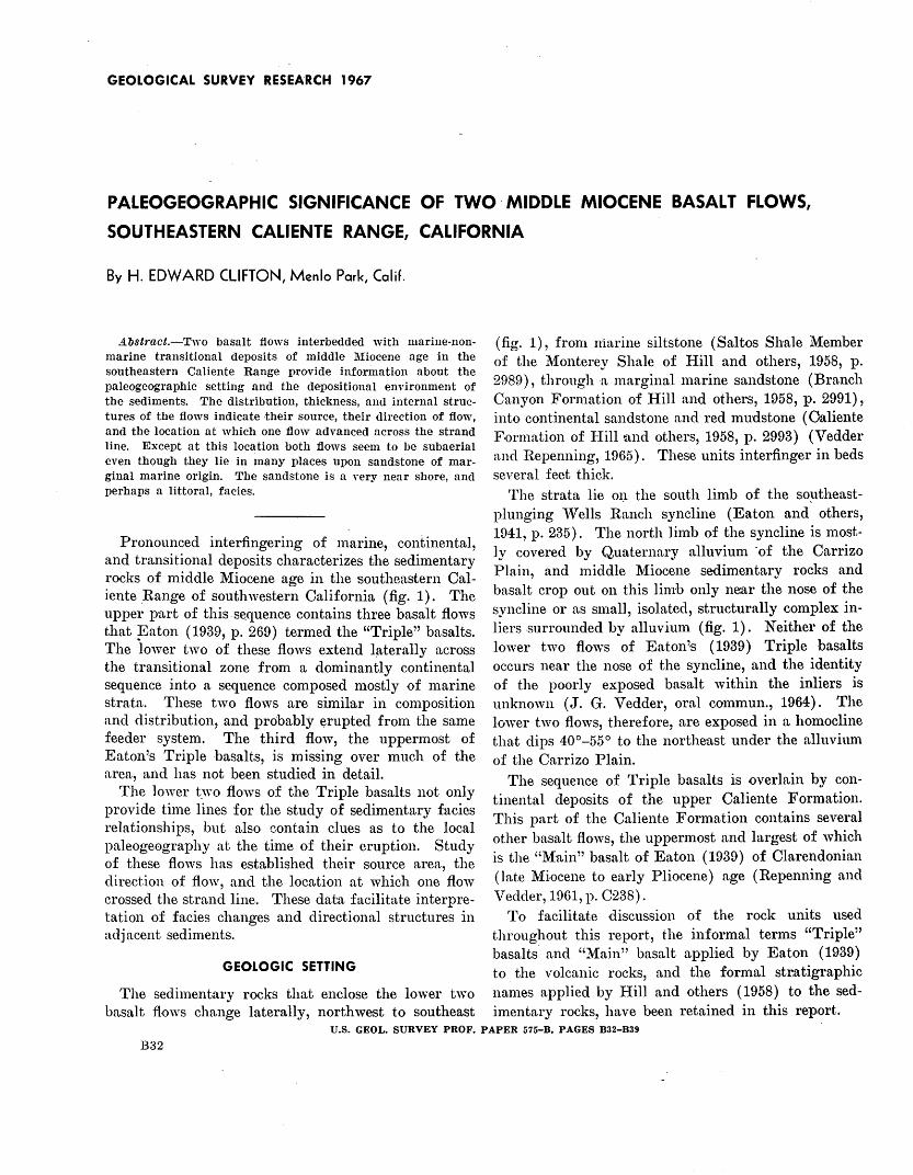
GEOLOGICAL SURVEY RESEARCH 1967

PALEOGEOGRAPHIC SIGNIFICANCE OF TWO· MIDDLE MIOCENE BASALT FLOWS,

SOUTHEASTERN CALIENTE RANGE, CALIFORNIA

By H. EDWARD CLIFTON, Menlo Park, Calif.

A.bstract.-Two basalt flows interbedded with marine-non­marine transitional deposits of middle Miocene age in the southeastern Caliente Range provide information about the paleogeographic setting and the depositional environment of the sediments. The distribution, thickness, and internal struc­tures of the flows indicate their source, their direction of flow, and the location at which one flow advanced across the strand line. Except at this location both flows seem to be subaerial even though they lie in many places upon sand·stone of mar­ginal marine origin. The sandstone is a very near shore, and perhaps a littoral, facies.

Pronounced interfingering of n1arine, continental, and transitional deposits characterizes the sedimentary rocks of middle Miocene age in the southeastern Cal­iente Range of southwestern California (fig. 1). The upper part of this s~quence contains three basalt flows that ~aton (1939, p. 269) termed the "Triple" basalts. The lower two of these flows extend l~terally across the transitional zone from a dominantly continental sequence into a sequence composed mostly -of marine strata. These two flows are similar in composition and distribution, and probably erupted from the same feeder system. The third flow, the uppermost o£ Eaton's Triple basalts, is missing over 1nuch of the area, and has not been studied in detail.

The lower t_wo flows of the Triple basalts not only provide time lines for the study of sedimentary facies relationships, but also contain clues as to the local paleogeography at the time of their eruption. Study of these flows has established their source area, the direction of flow, and the location at which one flow crossed the strand line. These data facilitate interpre­tation of facies changes and directional structures in aclj a cent sediments.

GEOLOGIC SETTING

The sedimentary rocks that enclose the lower two basalt fl.ows change laterally, northwest to southeast

(fig. 1), from niarine siltstone (Saltos Shale Member of the l\tfonterey Shale of Hill and others, 1958, p. 2989), through -a marginal marine sandstone (Branch Canyon Formation of Hill and others, 1958, p. 2991), into continental sandstone and red mudstone (Caliente Formation of Hill•and others, 1958, p. 2993) (Vedder and Repenning, 1965). These units interfinger in beds several feet thick.

The strata lie 01~ the south limb of the so~ltheast­plunging 'Vells Ranch syncline (Eaton and others, 1941, p. 235). The north li1nb of the syncline is most­ly covered by Quaternary alluvium ·of the Carrizo Plain, and middle Miocene sedimentary rocks and basalt crop out on this lin1b only near the nose of the syncline or as small, isolated, structurally complex in­liers surrounded by alluvimn (fig. 1). Neither of the lower two flows of Eaton's ( 1939) Triple basalts occurs near the nose of the syncline, and the identity of the poorly exposed basalt within the inliers is unknown (J. G. Vedder, oral commun., 1964). The lower two flows, therefore, are exposed in a homocline that dips 40°-55° to the northeast under the alluvium of the Carrizo Plain.

The sequence of Triple basalts is overlain by con­tinental deposits of the upper Caliente Formation. This part of the Caliente Formation contains several other basalt flows, the uppermost and largest of which is the "Main" basalt of Eaton ( 1939) of Clarendonian (late Miocene to early Pliocene) age ( Repenning and Vedder, 1961, p. C238).

To facilitate discussion of the rock units used throughout this report, the informal terms "Triple" basalts and "Main" basalt applied by Eaton (1939) to the volcanic rocks, and the formal str:atigraphic names applied by Hill and others (1958) to the sed­imentary rocks, have been retained in this report.

U.S. GEOL. SURVEY PROF. PAPER 575-B, PAGES B32-B39

B32

E X PLANATION

! r Undivided Q~~:~n~ry and Terti -;:S ary contmental depos1ts

'* ~Q ~ 1 " Mam " basalt

~ [kB 0.. Sandstone of Caliente Formation

f~)'s/l Caliente Formation

ltf~~t l Caliente and Branch Canyon

Forma tions -Branch Canyon Formation and Saltos Shale Member of Monterey Shale

~ Saltos Shale Member of

Monterey Shale

~ Triple basalts Tb3, upper flow Tb 2, m i ddle }low Tb, , lower flow

Appro ximately located contact -- 7

Stratig raphic section shown in figure 2

/

0

7

< /'

.6>

CLIFTON

,<:,

< "~;

• Wells Ranch

QTc

San Francisco 0

-1> 4-

.Area of /' report ""i

B33

N

l'v 05'

FIGURE 1.- l\Iiddle Miocene and post-middle Miocene rocks in the southeastern Caliente Range, Calif. (modified after Vedder and Repenning, 1965). Stratigraphic nomenclature is that of Eaton (1939) and Hill and others (1958).

B34 PALEONTOLOGY AND STRATIGRAPHY

DISTRIBUTION AND ·THICKNESS

The middle and lower flows of the Triple basalts extend continuously from the East Fork of Padrones Canyon to the western wall of Abbott Canyon (fig. 1), a distance of 1nore than 8 miles (Eaton, 1939; Vedder and Repenning, 1965). On the southeast, the lower flow pinches out in an area of poor exposures in the East Fork of Padrones Canyon, and the middle flow can be traced with certainty only a short distance far­ther eastward. On the northwest, the lower flow crops out intermittently nearly a mile northwest of Abbott Canyon (figs. 1 and 2), whereas the middle flow is not present beyond the western slope of the ridge west of Abbott Canyon.

The two flows lie in contact with either the Caliente or Branch Canyon Formations; they are nowhere in

NW

1 .

. .

.

.

11

Abbott Canyon

I I 3

12

4 Middle flow

Lower flow

Middle flow

Lower flow

0

contact with the Saltos Shale (fig. 2). In the south­east both flows are enclosed within continental sand­stone or mudstone of the Caliente Formation. To the northwest, both are overlain mostly by the Branch Canyon Formation, but whereas the middle flow over­lies sandstone of the Branch Canyon Formation, the lower flow rests mostly upon red and green mudstone of the Caliente Formation (fig. 2).

The thicknesses of the flows vary similarly (fig. 2). Both flows are thickest (100-140 ft) near the West Fork of Padrones Canyon, and thin rather abruptly to the southeast. Northwestward, they gradually thin to a minimum of 25-30 feet near section 9; just west of this point the thickness of the flows increases to 60-80 feet and remains nearly constant westward to the vicinity of Abbott Canyon. The thickness of the

5

West Fork Padrones Canyon

I

14 :

5000'

6

7 8

East Fork Padrones Canyon

116

Horse Canyon

I

10)

17

SE

EXPLANATION

~ - -Caliente Formation Branch Canyon Formation Saltos Shale Member Basalt Covered interval (continental) (marginal marine) of Monterey Shale

(marine)

FIGURE 2.-Stratigraphic cross section along the strike of the lower two flows of the Triple basalts of Eaton ( 1939). Location of numbered stratigraphic sections is shown on figure 1. ·

CLIFTON B35

sedimentary rocks between the :flows follows a some­what reciprocal pattern, being smallest on the south­east and increasing northwestward, although it, too, decreases locally near section 9.

In the vicinity west of the fork of Padrones Can­yon, the flows are accompanied by two less extensive ones (fig. 2, not shown in fig. 1 because of the small map scale). A basalt flow, as much as 40 feet thick, lies beneath the lowest flow of the Triple basalts and is separated from it by a lens of basaltic sandstone. Another flow, as ·much as 60 feet thick, overlies con­tinental sediments above the middle flow. Both of the smaller flows are discontinuous and of limited extent; the lower one crops out intermittently for nearly 3 miles and the uppermost for more than 1 mile.

In the west fork of Padrones Canyon, basaltic dikes as much as 3 feet thick intrude the sedimentary rocks beneath the Triple basalts. The dikes are nearly ver­tical and strike north. They are petrographically sim­ilar to the :flows, and, although not in contact with them, probably are part .of the system that fed the flows.

DESCRIPTION

The flows appear from a distance as dark-gray streaks intercalated with cream-colored sandstone beds of the Branch Canyon Formation and pastel mud­stones and sandstones of the Caliente Formation. The basalt is relatively resistant to erosi.on in the south­eastern part of the area, but relatively unresistant in the northwestern part.

The flows typically are dark gray and speckled near the top and bottom by white amygdules. The basalt weathers to a monotonous hackly surface which is in­terrupted by zones as much as 20 feet wide containing resistant basalt spheroids which range from a few inches to several feet in diameter (fig. 3). Except f.or the spheroidal masses, the outcrops generally are covered with a thin layer of basaltic debris. The flows commonly have a partly stratified aspect resulting from platy partings and alternating layers of differ­ent resistance to weathering (fig. 4) .

The lower contact of the flows is generally planar, although in a few places the basalt seems to have Slmk into the underlying sediment or to have been injected at the base by small amounts of sediment. Such features are analogous to the load casts and :flame structures of sedimentary rocks. ·where red mudstone underlies the flow, the color of the mudstone is intensified along the contact. In most places where sandstone underlies the flow the uppermost few inches are generally red or purple, but in the northwestern part of the area most of the sandstone under the middle flow is uncolored.

FIGURE 3.-Middle flow of the Triple basalts near section 15 (figs. 1 and 2). Note resistant spheroids in central part of flow. Tb,, middle basalt flow of the Triple basalts; Tc, Caliente Formation.

The tops of the flows show evidence of erosion. Over­lying mudstone contains coarse angular basalt rubble in the lower foot or so. Where sandstone overlies a flow, the rubble is absent and the sandstone lies directly on the flow, filling irregular cracks and pockets. Isolated basalt fragments are common, however, in such sand­stone.

COMPOSITION AND TEXTURE

Originally the flows consisted of 5-20 percent euhedral phenocrysts and granules of high-magnesium olivine, 10- 15 percent plagioclase phenocrysts (AnwAn60), 25-45 percent plagioclase microlites (An50-An55 ), 0-25 per­cent titaniferous subcalcic (2V=30°-40°) augite, 5-10 percent opaque iron-titanium oxides, 0-55 percent dark­brown glass, and 0-10 percent interstitial voids.

The original mineral.ogy of the flows is considerably altered. A clay mineral of the montmorillonite group in most places forms pseudomorphs after the olivine. Plagioclase commonly is partly to completely altered to celadonite, which also occurs interstitially, probably as a void-filling. The glass is devitrified to a slightly birefringent, very fine grained aggregate. Calcite commonly replaces olivine, plagioclase, and glass near the base of the flows and, particularly, at the western terminus of the middle flow. Augite, in contrast to the other primary minerals, shows no sign of replace­ment or alteration.

The texture of the basalt depends upon its location within the flow. The texture is hyalophitic at the bottom and top of the flow. Here, devitrified glass encloses small olivine and plagioclase microlites, and augite is :absent, as it is wherever the basalt has been

B36 PALEONTOLOGY AND STRATIGRAPHY

l<~IGURE 4.- Lower flow of the Triple basalts near section 10 (figs. 1 ancl2). Note banding in upper part of flow. Tb,, basalt flow; Tcb, Caliente and Branch Canyon Formations.

chilled. Augite first occurs as microlites in the basal 6 inches .or upper 3 feet of the flow, and increases in abundance within a foot or so toward the center of the flow to form a subophitic or ophitic texture. The dis­tribution of augite-particularly its absence from the chilled basalt at the western end of the middle flow -indicates that it did not begin to crystallize until movement had ceased.

STRUCTURES

The flows contain these primary structures : vesicles, pipe vesicles, contraction joints, indistinct flow band­ing, and locally, pillows.

Most vesicles now are amygdules consisting of either calcite or montmorillonitic clay minerals, although a few consist of calcite rimmed by radially fibrous clay minerals. Most amygdules are about half an inch across, although some are as much as 2 inches long. Their shapes. range from spheroids to irregular knob­by masses; knobby :amygdules are equally abundant in the tops and bottoms of the flows. In general, the amygdaloidal zones extend for 2 to 3 feet below the top of a flow and for half a foot to 1 foot above the base. Locally, amygdaloidal layers several inches thick a lso .occur in the flow interior, but such layers lack lateral persistence. Some larger cavities, as much as several inches long, are partly filled with drusy quartz or calcite, but they occur only locally.

A few pipe vesicles, vertical tubes half an inch to 1 inch in diameter and as much as several feet long, occur in the lower half of the flows. The tubes are either empty or filled with disintegrated basalt. The

tops of the tubes commonly are bent in the direction of flow.

Contraction joints a quarter of an inch to 1 inch wide, filled with a friable mixture of calcite and mont­morillonitic clay minerals, are abundant in the lower part of the flows. Most of these joints curve upward randomly and join an anastomosing network of simi­lar joints in the flow interior. Similar fractures in the upper part of the flow tend to parallel the upper flow surface. Basalt in contact with the joints is finer grained than that several inches away, indicating formation of the joints before complete crystallization. The joints ·are not uniformly deflected from the base, however; therefore, they probably developed after flowage had ceased.

An indistinct horizontal banding appears in the basalt at many places (fig. 4). The banding, which reflects variation in the degree of alteration and weathering of the basalt, results from alternating zones of different resistance that may be due to un­equal volatile concentrations in zones of internal shear during flowage.

vVell-shaped pillows occur only at the western terminus of the middle flow, and are described in de­tail later since they relate to the movement of the flow -across the strand line. Other structures, similar to poorly defined, possibly incipient, pillows, occur in numerous places near the base of the flows. They are outlined by spheroidal clusters of amygdules or by anastomosing contraction joints. They are probably not pillows, however, for the basalt in the amygda­loidal clusters is texturally similar to the nonvesicular rim; this similarity suggests that internal volatile concentration, not external chilling, caused the struc­ture. Resistant spheroids that are common on ex­posures of the basalt have a pillowlike appearance but probably are weathering phenomena. They are distinctly less altered than the surrounding rock but show no textural difference.

SOURCE OF FLOWS

Much evidence indicates that both flows originated near the present West Fork of P:adrones Canyon (sec­tions 14 and 15, figs . 1 and 2) . Here the flows reach their greatest thickness and are associated with small local flows. Nearby subjacent dikes of similar ba­saltic composition suggest a feeder system. In addi­tion, the partly volcaniclastic rocks between the flows imply nearby volcanism.

A lens .of basaltic sandstone as much as 50 feet thick separates the lower flow of the Triple basalts from the thin, local, flow beneath it. More than half of this sandstone consists of altered basalt clasts

CLIFTON B37

ranging in size from fine sand to blocks several inches across. Basalt in sand-size grains is much more glassy and vesicular than in the flows :and commonly contains grains of detrital quartz. Nearly all the basaltic grains are intensely oxidized and appear bright red in transmitted light. The grains probably formed while the basalt was still fluid, for many have an opaque, unvesiculated rim that completely envelops them. Moreover, some seem to have been deformed while pliruble, because stretched vesicles conform with the shapes of the grains (fig. 5). Olivine phenocrysts, now replaced by a tan clay mineral of low bire­fringence and refractive index, have "charred," nearly opaque rims which suggest strong oxidation prior to and during eruption. These features indicate that the basaltic grains are lapilli ejected under hot, oxidizing conditions. Their concentration in these beds indi­cates that the vent was nearby.

The lapilli have been reworked, for they are mixed with a considerable amount of nonvolcanic detritus, and the larger basalt fragments proba:bly were derived from erosion of the lower local flow. Broken oyster shells, probably derived from nearby marine deposits, are scattered through the sandstone, which also has yielded a jaw fragment of :a Miocene felid (C. A. Repenning, oral commun., 1965).

A different type of pyroclastic material also occurs in this vicinity. Both the middle and lower flows of the Triple basalts are locally overlain by bentonitic mudstone as much as 2 feet thick. Glass shards in the mudstone, :altered to a montmorillonitic clay, attest to its pyroclastic origin. The mudstone also contains vesicular basaltic clasts as much as several inches across that contain much altered basaltic glass. Plagioclase microlites in the glass are much smaller than those in the flows. Chilled rinds enveloping these fragments indicate that they, too, are ejecta, and their presence in a volcanic ash bed suggests direct pyroclastic activity.

In summary, the lower and middle flows of the Triple basalts emanated from :a source very near the West Fork of Padrones Canyon. This interpretation differs from that of Eaton and others ( 1941, p. 225), who surmised that the flows "originated several miles northeast of the present "\V ells Ranch" (fig. 1).

DIRECTION OF FLOW

Evidence of flow direction ("\Vaters, 1960) IS

meager. The best indication occurs in the lowermost part of the flows, where amygdules locally are inclined with respect to the flow base. Where oriented, they consistently are elongate in a generally west-southwest direction and plunge toward the east. Such inclina-

l<'IGUHE [).-Photomicrogroph of basaltic sandstone below the lower flow of the Triple basalts near section 14. Note de­formed Yeh icles (V), detrital quartz in basaltic grains (Q), chilled rim on basaltic grain (R), and opaquely rimmed relict oliYine phenocrysts ( 0). X 25.

tion generally is toward the source (Waters, 1960, p. 360) and in this area indicates flowage to the west and southwest (fig. 6), with :a hint of fanning from a postulated vent just north of the present West Fork of Padrones Canyon. The only other indication of flow direction, the westward deflection of pipe vesicles (Waters, 1960, p. 358), supports the idea of lava flow­age toward the west.

Paleocurrent data from a fluviatile sandstone (Tcs on fig. 1) in the upper part of the Caliente Formation substantia.te this interpretation of locaJ paleoslope. The sandstone disconformabJy overlies the middle Miocene strata that contain the basalt flows. It has yielded no diagnostic fossils but grades upward into strata that bear fossil ,·ertebrates of Clarendonian a.ge (Repen­n ing and Vedder, 1961, p. C238). Therefore, the age of the sandstone is probably late Miocene (Mitchell and Repenning, 1963, p. 15; Evernden and others, 1964, fig. 1), and the hiatus separating it. from middle Mio­cene strat.a. is likely minor. Pebble imbrication (fig. 6) in this sandstone as well as a consistent westward de­crease in clast size, indicate a paleoslope direction simi­lar to that suggested by the structures in the basalts and establish a local paleoslope toward the west-southwest.

POSITION OF THE STRAND LINE

The lower flow of the Triple basalts lacks pillows or breccia indicative of subaqueous flow and seems everywhere to be subaerial. So, for nearly its full extent, does the middle flow, even though it rests upon sandstone of the Branch Canyon Formation for more than half its length (fig. 2). Near Abbott Canyon, however, the middle flow contains many features that

B38 PALEONTOLOGY AND STRATIGRAPHY

N

. ./

FIGURE 6.-Direction of flow (arrows) of the low~r two flows of the Triple basa'its as indicated by amygdule orientJation. Rose diagram (inset) shows direction of currents that de­posited sandstone of the Caliente Formation (Tcs, fig.1), based on measurements of pebble imbrication in 98 beds.

suggest that it here crossed the strand line (fig. 7) : pillows near the bottom and top of the flow, breccia at its base, and numerous geodes as much as 3 inches across that are partly filled with quartz or calcite. The basalt adjacent to the geodes is chilled, indic-ating that they were large primary cavities, probably formed by expanding steam.

Pillows near the bottom of the middle flow are ex­posed under a veneer of basaltic debris on the ridge­top west of Abbott Canyon (sec. 2). The pillows are isolated, generally less than a foot across, and flat­tened parallel to bedding. Many contain a geode or large amygdule in their upper part. Each pillow has a yellowish chilled margin about a quarter of an inch thick. The matrix between the pillows contains much more :altered glass than the basalt in the pi,llow in­teriors. The matrix may be basalt breccia, but samples sufficiently large to demonstrate fragmenta­tion could not be obtained because of thorough de­composition of the material.

A cluster of pillows also occurs in the upper 8 feet of the flow about 500 feet west of this ridge top, at a

point where the flow thickness abruptly decreases to­ward the west (fig. 2}. These pillows, as much as 3 feet in diameter, are larger than those at the base. Individual pillows are separated· 'by an envelope of sandstone, and the basalt in cont-act with the sand­stone is chilled. A few yards west of the pillows, the upper surface of the flow is quite irregular and suggests invasion into loose wet sand, possibly heaped onto the front of the advancing lava. ·

The flow at this point rests on sandstone that con­tains impressions of marine mollusks, and the lower­most foot of basalt is brecciated. West ward the ba­salt continues to thin (fig. 2) and grades late.rally from a thin, glassy basalt flow with a brecciated base, through basaltic breccia, into basaltic sandstone. The basaltic sandstone bed, little more than a foot thick, becomes progressively diluted by terrigenous material ·and can be traced as a distinct bed for only about 100 feet.

In summary, indications of lava passage into the marine environment exist only in the middle flow at its western end. The lava appears to have crossed the strand line at a point near the ridgetop west of Abbott Canyon. Sand-encased pillows at the top of the flow suggest that the flow plowed under wet sand as it advanced into the water.

CONCLUSIONS

The lower and middle flows of the Triple basalts erupted near the West Fork of Padrones Canyon and flowed toward the west-southwest. Directional prop­erties of slightly younger fluviatile sandstone indicate a similar local paleoslope. The depositional strike of sediments deposited in this area during the middle Miocene, which can be considered to be normal to this paleoslope, serves as a base relative to which features of the sediment such as directional structures and facies change can be interpreted. The middle flow crossed the strand line near the terminus of the flow just west of Abbott Canyon; otherwise neither flow

SE

0

200'

FIGURE 7.-Features at the western end of the middle flow of Ea,ton's ( 1939) Triple basalts. For location -see figure 1.

CLIFTON B39

shows evidence of having flowed into water. The middle flow extensively overlies sandstone of the Branch Canyon Formation, as does the lower flow locally; much of the marginal marine sandstone of the Branch Canyon Formation is therefore thought to have been subaerially exposed during at least part of middle Miocene time.

REFERENCES

Eaton, J. E., 1939, Geology ~nd oil possibilities of Caliente Range, Cuyama Valley, and Carrizo Plain, California: California Jour. Mines and Geology, v. 35, no. 3, p. 255-274.

Eaton, J. E., Grant, U. S., and Allen, H. B., 1941, Miocene of Caliente Range and environs, California : Am. As:soc. Pe­troleum Geologists Bull., v. 25, no. 2, p. 193-262.

Evernden, .J. F., Snvage, D. E., Curtis, G. H., and James, G. T., 1964, Potassium-argon dates and the Cenozoic mammalian

chronology of North America: Am. Jour. Sci., v. 262, p. 145-198. .

Hill, M. L., Carlson, S. A., and Dil~b~ee,. T. W., Jr., 1958, Stratig­raphy of Cuyama Valley-Caliente Range area, California: Am. Assoc. Petroleum Geologists Bull., v. 42, no. 12, p. 2973-3000.

Mitchell, E. D., Jr., and Repenning, C. A., 1963, The chronologie and geographic range of desmostylians: Los Angeles County Museum Contr. in Sci., no. 78, 20 p.

Repenning, C. A., and Vedder, J. G., 1961, Continental verte­brates and their stratigraphic correlation with marine mol­lusks, eastern Caliente Range, California: Art. 235 in U.S. Geol. Survey Prof. Paper 424-C, p. C235-C239.

Vedder, J. G., and Repenning, C. A., 1965, Geologic map of the southeastern Caliente Range, San Luis Obispo County, Cal­ifornia: U.S. Geol. Survey Oil and Gas Inv. Map OM-217, scale 1 : 24,000.

\Vaters, A. C., 1960, Determining direction of flow in basalts: Am. Jour. Sci., v. 258-A (Bradley Volume), p. 350-366.

GEOLOGICAL SURVEY RESEARCH 1967

MICROFOSSIL EVIDENCE FOR CORRELATION OF PALEOCENE STRATA

IN BALLARD COUNTY, KENTUCKY,

WITH THE LOWER PART Of THE PORTERS CREEK CLAY

By S. M. HERRICK and ROBERT H. TSCHUDY, Atlanta, Ga., Denver, Colo.

·Work dane in cooperation with the Kent'ucky Geological Survey

Abstract.-Foraminiferal and palynological evidence suggests an early Porters Creek age for deposits in northern Ballard County, Ky. Comparison with microfaunas described from localities in the Gulf Coast and Mississippi embayment regions indicates an horizon above the Clayton and in the basal part of the Porters Creek that is equivalent to Plummer's "transi­tion zone" (Paleocene of Texas) and to Kellough's Polymor­phina cushmani zonule 1n the basal part of the Wills Point Formation (Paleocene of Texas).

The purpose of this paper is ( 1) to record the pres­ence of certain Fora-minifera and palynomorphs (pollen, spores, :acritarchs, al).d dinoflagellates) from an exposure in northern Ballard County, l{y., (2) com­paring these Foraminifera and palynomorphs with previously described assemblages from other parts of the Gulf Coast and the Mississippi embayment region, and ( 3) to suggest the nature of the environment under which the sediments yielding these fossils were deposited.

Two samples were collected by W. W. Olive, of the U.S. Geological Survey, in Ballard County, Ky., from an exposure of Paleocene deposits on the bank of the Ohio River (fig. 1), 0.5 mile below the landing at Olmsted, Ill. (Kentucky coordinates S1,030,700-323,120) . . Sample Od-2, taken from an altitude of 295 feet, was a dark-greenish-gray, silty, micaceous, sparsely gla-uconitic clay that yielded palynomorphs. Sample Od-1, taken from an altitude of 286 feet~ was much sandier and more abundantly glauconitic and phosphatic, and it yielded both Foraminifera and palynomorphs. Other fossils observed in the samples were some unidentified fish teeth. U.S. Geological Survey paleobotanical locality numbers D-3691 and

D-3692 were assigned to samples Od-2 and Od-1, respectively.

C. L. Cooper apparently was the first to publish on the Foraminifera from the northern part of the Mississippi embayment. Cooper (1944) described and illustrated :a fauna derived from cuttings from a well drilled in 1938 near Cache, Alexander County, Ill. These fossils, with some tax.onomic changes by the authors, are listed under locality 2 in table 1. On the basis of the species identified from these well cuttings, Cooper concluded that 'this fauna was of Porters Creek age.

Pryor and Ross (1962, p. 24) assigned an 18-foot clay bed of a measured geologic section in Pulaski County, in southern Illinois, to the Clayton Formation on the basis of the foraminifer, Globigerinoides daub­.1ergensis. However, this fossil occurs throughout the Paleocene of the Atlantic and Gulf Coasts (Loeblich and Tappan, 1957, p. 185); consequently, it is not diagnostic of the lower unit (Clayton or Kincaid) of the Paleocene of North America. Pryor and Ross noted that. material from about 4 to 11 inches from the base of the 18-foot clay bed was very sandy. On the basis of field evidence, W. W. Olive (written commun., 1965) considers this basal sandy horizon of Pryor and Ross to be the probable equivalent of a 4-foot fossiliferous sandy clay containing the 286-foot horizon herein discussed.

Browne and Herrick (1963) described and illus­trated a Paleocene foraminiferal fauna from an out­crop near Reidland, McCracken County, Ky., and concluded that this fauna was of probable Porters Creek age.

U.S. GEOL. SURVEY PROF. PAPER 575-B. PAGES B46-B44

B40

HERRICK AND TSCHUDY B41

go• sa· 38·.--~ ,'1 -~..l' -/-1

'.._ I L L I N 0 I S )J '..J

'\\ ALEXANDER \

'-h:~TY . ;--__)

MISS 0 URI:·:::·:·<\f~:;.:., ·::. KENTUCKY

: . ·. 2(BALLARD . ·.· • J COUNTY r~-:-·.".

--.:7~ ~~--_J,-4t . . '\ ? CALLOWAY · .··

;_;~ COUNTY ..

,., __ /\ ·.· ~ ( T E

1---,~ ... A R K A N S A S ~LAUDERDALE

· <'- COUNTY

'------1

~ I

E S S E E

) ;' .

;---- UNI0:----~:.7" '\ COUNTY · 1· · >.

/ . c_-_x_v r··ALABAMAJ

.f M I S S I S S I P P I : : ·_.:·u_:_:. i / I ... l I ··:::: 34 °

0 50 100 MILES

EXPLANATION

FOSSIL LOCALITIES

.2 xl Mississippi embayment area Well Outcrop

FIGUIU<~ 1.-J.,ocation of fossil localities referred to in text.

Although there is almost a complete lack of pub­lished information on palynology of Paleocene rocks of the Mississippi embayment region, an exception is a paper.by Jones (1962) in which some of the palyno­logical characteristics of the Porters Creek Clay and t.he Wilcox Group in south-central Arkansas are dis­cussed. In a. 70-foot Porters Creek sequence, Jones found taxodiaceous pollen to be the dominant form present. l-Ie reported also the presence of the genus Aq'ldla]Jollenites. This genus, until recently, had not been found in rocks of the northeastern part of the embayment. Jones noted the similarity of some of his fossils to Paleocene fossils from other regions, but no closer age determinations were drawn.

AGE IMPLICATIONS

Foraminifera

In using Foraminifera as age indicators, known ranges for the individual species are usually satisfac­tory in an :analysis of this kind. In this paper, the Foraminifera listed in table 1 were compared with the sa;me species as previously reported by. Plummer

(1926). The Foraminifera from the. 286-foot horizon of locality 1 were considerably leached but were · sufficiently well preserved to permit identification of approximately 45 species.

With the exception .of V aginulina. gracilis, which according to Plummer (1926, p. 23-24) characterizes the lower part (Kincaid) of the Paleocene in Texas, the species listed in table 1 are pf Porters Creek age.

TABLE 1.-Paleocene Foraminifera from Kentucky and Illinois

Locality 1 1 Locality 2 3 (Ballard. (Alexander

County, Ky.) County, Ill.)

Clavnlinoides midwayensis Cushman____ X _________ _ Robulus degolyeri (Plummer) .. _ .. _______ X _________ _ R. inornatus (d'Orbigny) ______________ ----~----- X R. magnificus Toulmin· ________________ ---------- X R. midwayensis (Plummer) ___________ - X X R. pseudomarnilligerus (Plummer)______ X _________ _ Marginulinaearlandi (Plummer) _______ X ----------Dentalina aculeata d'Orbigny _ _ _ _ _ _ _ _ _ _ X _________ _ D. colei Cushman and Dusenbury _____ - _ _ _ _ _ _ _ _ _ _ X D. delicatula Cushman ________________ X _________ _ D. pauperata d'Orbigny _______________ ---------- X D. plummerae Cushman _______________ X ----------D. vertebralis (Batsch) var. albatrossi?

(Cushman)________________________ X Nodosaria ajfinis Reuss_______________ X N. latejugata GUmbeL _______________ - X N. ? cf. N. longiscata d' Orbigny________ X N. ? spinocostata Cooper_ _ _ _ _ _ _ _ _ _ _ _ _ _ X Chrysalgoniurn eocenic1tm Cushman and Todd _____________________________ X

X X

X

C. granti (Plummer)__________________ X 'Pseudonodosaria laevigata (d'Orbigny)

var. occidentalis Cushman ___________ X -----------Vaginulina gracilis Plummer_________ X X V. midwayana Fox and Ross__________ X X Lagena laevis (Montagu) _________________ · _______ X Guttulina problema d'Orbigny __________ X X Globulina gibba d'Orbigny _____________ X ----------Polymorphina wshmani Plummer______ X X P. subrhombica Reuss ________________ X _________ _ Bullopora ? laevis (Sollas) _ _ _ _ _ _ _ _ _ _ _ _ _ X - _--------Spirobolivina scanica (Brotzcn) _ _ _ _ _ _ _ _ X _________ _ Rectoguembelina alaba mensis Cushman_ _ _ _ _ _ _ _ _ _ _ _ X Siphogenerinoides eleganta (Plummer)___ X X B1tliminella elegantissima (d'Orbigny) ___ X ----------B. cacumenata Cushman and Parker ____ X ----------Bolivina midwayensis Cushman________ X _________ _ Pleurostomella paleocenica Cushman____ X _________ _ Stilosomella midwayensis (Cushman and Todd) ____________________________ X

S. paleocenica (Cushman and Todd)____ X S. phtmmerae (Cushman)_____________ X Gyroid1:noides aequilateralis (Plummer)__ X Eponides phtmmerae Cushman_________ X Pulsiphonina prima (Plummer)________ X Epistominella cf. E. viirea Parker a_____ X Alabamina wilcoxensis Toulmin _ _ _ _ _ _ _ _ X Pullenia Q1tinqueloba (Reuss) var.

angusta Cushman and Todd_________ X Globigerina triloculinoides Plummer_____ X Globigerinoides daubjergensis (Bronni-

mann) ____________________ ~------- X Globorotalia compressa (Plummer)______ X Anomalinoides acuta (Plummer) ________ X A. midwayensis (Plummer) ____________ X Cibicides vulgaris (Plummer)__________ X

X X X

X

X

X

X X X X

Cibicidoides alleni (Plummer) __________ ---·------- X

1 Identified by S.M. Herrick,_(this paper); sample Od-1 (286-foot level). 2 Identified by Cooper (1944, pls. 54, 55), with some taxonomic changes (this paper). J Identified by Ruth Todd.(this paper), U.S. Geological Survey, Washington, D.C.

B42 PALEONTOLOGY AND STRATIGRAPHY

Elsewhere in the Mississippi embayment these species occur in the upper and lower units of the Midway Group, are confined to the upper unit of the Midway, or occur in formations that are geologically younger than Midway. 'Of the species listed in table 1, four are considered here as significant indicators of the geologic age of these deposits. These include Robulus p.r:;eudomamilligerous, Polymorphina cushmani, Oibi­cides vulgaris, and Cibicidoides alleni. All four are regarded by Plummer (1926, p. 98, 125, 145) as indi­cative of the "transition zone," an horizon she places between the upper (Wills Point Formation) and lower (Kincaid Formation) units of the Texas Paleocene. Kellough ( 1959, fig. 7) gives the Foraminifera com­posing this unique fauna the name "Polymorphina cushmani zonule" and places it in the basal part. of the Wills Point of the Paleocene section as exposed along Tehua~ana Creek, Limestone County, Tex.

The three species, V aginulina gracilis, Nodosaria ~ spinocostrata, and Epistominella cf. E. vitrea prob­ably should be added to this group. Regarding V. gracilis as an indicator of her "transition zone," Plum­mer ( 1926, p. 111) states, "In the areas where a nar­row zone of transition lies between the basal and upper beds, V. gracilis dies out through these few feet of section as the upper form, V. midwayana becomes more and more abundant ... " In the 286-foot horizon V. gracilis occus rarely, whereas V. midwayana is rather numerous-a condition similar to that reported by Plummer ( 1926, p. 21, 111) in the region north and northeast of the Mexia area, Texas, where this faunal transition prevails in the Texas Paleocene section. Nodosaria ? spinocostrat.a, its stratigraphic range yet to be established, was described by Cooper ( 1944, p. 349) :as a new species. This species may represent a variant of Stilostomella 1nidwayensis. However, until appropriate comparisons have been made, this species is here regarded as distinct and as a possible indicator of early Porters Creek age in the northern part of the embayment. Epistominella vitrea was described by Haynes (1956, p. 88) from the upper Paleocene ( Thanet beds) of East Kent, England. Its presence in the "transition zone" of the Paleocene sequence in Ballard County, Ky., is interesting, though its strati­graphic significance in this part of the embayment remains to be determined. On the basis of this for am­iniferal comparison, the age of the 286-foot horizon in Ballard County, Ky., is early Porters Creek.

Plant fossils

So that the fossil pollen and spores in the two Ballard County samples similarly might be used for correlation purposes, the U.S. Geological Survey

palynological laboratory in Denver, Colo., determined the micro:floral content of "control" samples collected from well-dated sections of the Clayton Formation and of the Porters Creek Clay. ·

The control samples of the Clayton were collected in the SY2NW14 sec. 8, T. 6 S., R 3 E., from an ex­posure in the southwest wall of a tributary to Guyton Creek in Union County, Miss. This exposure, which is shown as locality 4 in figure 1, is along a county road 1.5 miles south-southwest of the town of Cotton Plant and is in an area mapped geologically by Conant ( 1942) as Clayton. The samples yielding abundant and well-preserved microfossils were given U.S. Geological Survey paleobotanical location num­bers D1966A, B, C, and F.

Although sampled in several places, the Porters Creek Clay generally yielded only a few very small palynomorphs or only finely divided organic remains. However, a sample (OHA-2) suitruble for use as a control was obtained from the channel of McCollough Fork, 300 -feet north of the Kentucky-Tennessee State line, Hazel quadrangle, Calloway County, Ky. (Ken­tucky coordinates S1,263,500-70,250). This sample

·was given U.S. Geological Survey paleobotanical locality number D-3285, and the site of collection is shown on figure 1 as locality 3.

Table 2 lists the percentage occurrence of groups of plant microfossils in the Clayton and Porters Creek control samples and in the two samples from the Ballard Oounty exposure (D-3691, D-3692). The Ballard County samples contained corroded but never­theless easily recognizable pollen grains and a few spores intermixed with well-preserved marine dino­flagellates and acritarchs. These assemblages were in contrast to the assemblages from Clayton control samples which yielded, in addition, an abundance of bisaccate conifer pollen that is poorly represented in the Ballard County samples.

As shown in table 2, the percentage of several microfossil groups in the control samples from the Clayton Formation and Porters Creek Clay differed markedly. Compared to the sample from the Porters Creek, the composited sample from the Clayton con­tained much smaller percentages of monosulcate, t~icolpate, and tricolporate pollen and much larger percentages of bisaccate conifer and taxodiaceous pollen. Moreover, the composited sample from the Clayton contained 160 code species/ whereas the Por­ters Creek control sample and the two Ballard County samples together contained 106. Only 4 of the code

1 Many of the species have not been named formally. For the pres­ent both those named and not named have been given temporary code designations and a "type" specimen of each has been placed on file In the U.S. Geological Survey paleobotanical laboratory In Denver, Colo.

HERRICK AND TSCHUDY B43

T ABLl!l 2.-Comparison of percentages of total pollen and spores found in control samples and in samples from Ballard County, Ky.

[ Percentngcs computed from specimen counts l;ly R. H. Tschudy, U.S. Geological Survey]

Locality 4 Locality 3 Locality 1 (Union (Calloway (Ballard

County, Miss.) County, Ky.) County, Ky.) ----------

Plant microfossil groups Clayton Porters Formation Creek Clay Od-1 Od-2

control control (286-ft (295-ft samples sample

com posited altitude) altitude)

DHI66 D3285 D3692 D3691 -------

Monolete spores ______ 1.2 ---------- ------- -------Trilete spores _________ 3.9 2.0 3.5 1.5 :Monosulcate pollen ____ 5.4 12.0 13.0 8 .. 5 Triporate pollen ______ 37.4 33.0 35.5 42.0 Arcoid tripornte pollen_ 1.5 2.0 3.5 .5 Tricolpate pollen ______ 9.2 22.5 17.0 14.5 Tricolporate pollen ____ 9.7 17.0 15.0 16.5 Brevitricolporatq pollen _____________ 1.9 .5 .5 .5 Bisaccate conifer pollen _____________ 15.0 1.5 2.5 2.0 Taxodiaccous pollen ___ 6.0 Other pollen and

3.0 3.0 2.5 spores _____________ 8.8 6.5 6.5 11.5

100.0 100.0 100.0 100.0 ---

Total count exclusive of dinofingellates and acritarchs ______ 600 400 200 200

species found in the Porters Creek samples were not found in the Clayton, and more than 50 code species found in the Clayton were not found in the Porters Creek. Furthermore, the 4 samples from the Clayton contained an average of 66 code species, the single sample from the Porters Creek contained .54, and of the two Ballard County samples one contained 54 and the other 41. Thus the :available evidence indicates a decline in the number of different species living in the Mississippi embayment area fr.om Clayton to Por­ters Creek time. This decline accords with other evi­dence that a decrease in the number of plant species in the embayment area began with the end of the Cretaceous and continued through the Paleocene.

Uecently, a sidewall core sample was obtained from the upper part of the Porters Creek sequence in a hole drilled for the U.S. Geological Survey in Lauder­dale County, Tenn., (locality 5, fig. 1). The Porters Creek sequence, according to the authors' interpreta­tion of the electric log, extends from depths of about 1,720 feet to about 2,350 feet. The sidewall core sample, which was from a silty layer at :a depth of 1,803 feet, yielded, specimens of Thomsonipollis and Aquilapollenites. The former is present in the upper ~aleocene N aborton Formation of Louisiana and commonly is found in samples of upper Paleocene and

241-334 0--67----4

lower Eocene sediments in the northern part of the embayment region. Aquilapollenites previously had been reported by Jones ( 1962) from the Porters Creek of Arkansas. This genus occurs commonly in Upper Cretaceous rocks of the Rocky Mountain region, but has not been found in the Cretaceous or lower Ter­tiary rocks of the Mississippi embayment region other than from these two localities. It appears unlikely that specimens of Aquilapollenites from the 1,803-foot level in the Lauderdale County well were redeposited. Several clumps made up of dozens of specimens were found, indicating deposition of whole anthers rather than disseminated pollen grains. During redeposition these anthers certainly would have been broken apart. The presence of Aquilapollenites in Jones' (1962) Porters Creek material suggests that his samples were from the upper part of the Porters Creek Clay.

The samples from the Ballard County exposure clearly pertain to the Porters Creek rather than to the Clayton, and the absence of late Paleocene genera such as Aquilapollenites and Thomsonipollis point to a lower Porters Creek stratigraphic position. The foraminiferal evidence obtained from the 286-foot level not only confirms this hypothesis but also pro­vides a tie with Plummer's "transition zone" between the Kincaid and Wills Point Formation of the Paleo­cene of Texas.

ENVIRONMENT OF DEPOSITION,

From the F.oraminifera and lithology of the 286-foot horizon, the ecologic environment under which this material was deposited doubtlessly involved a rather warm, shallow-water shelf or epeiric sea. This is de­duced from the sandy nature of the clay containing the Foraminifera as well as by the relative scarcity of pelagic F.oraminifera, the latter as noted by Plum­mer (1926, p. 12) and substantiated by the foramini­feral species listed in table 1.

In addition to the Porters Creek Clay samples dis­cussed herein, at least 10 other Porters Creek Clay samples from the northern embayment region have been examined. These yielded only finely divided organic fragments and a few small pollen grains. All the organic matter was nearly the same size, ranging from abou~ 5 to about 20 microns in diameter. This suggests winnowing, and deposition of the small-sized organic fraction along with clay at a distance from the margins of the basin. The three Porters Creek samples reported herein all yielded good suites of plant microfossils, although many were somewhat corroded. Large-sized spores and pollen were few but conspicuous by their scarcity. This, with the sandy nature of the clay, suggests a nearer shore deposition

B44 PALEONTOLOGY AND STRATIGRAPHY

site than that of the more winnowed nearly barren other Porters Creek samples.

The presence in both the Clayton and Porters Creek samples of acritarchs and dinoflagellates indigenous to a marine basin indicates marine deposition. Large­sized and abundant pollen and spores in Clayton samples indicate nearshore deposition. With the ex­ception of the sidewall core sample from the Lauder­.dale County well (which yielded no marine forms), the Porters Creek samples yielded a larger number and higher proportion of marine forms than did the Clayton.

CONCLUSIONS

Correlation of the Ballard County exposure· with the Porters Creek Clay rather than with the Clayton Formation is indicated by both the forami~iferal and palynological :assemblages. Furthermore, correlation with Plummer's "transition zone" betweenthe Kincaid and Wills Point Formations and with Kellough's Polynwrphina cushmani zonule in the basal Wills Point of the Texas Paleocene is based on foramini­feral similarities. The lack of upper P:aleocene genera such as Aquilapollenites and Thomsonipollis in the Ballard County exposure indicates correlation with the lower and not the upper part of the Porters Creek. The sandiness and the relative scarcity of pelagic

Foraminifera at the 286-foot horizon of the Ballard County exposure suggest that the depositional en­vironment was a shallow-water, shelf epeiric sea.

REFERENCES

Browne, R. G., and Herrick, S. M., 1963, Smaller Paleocene Foraminifera from Reidland, Kentucky : Bull. Am. Paleontology, v. 46, no. 210, p. 247-284, pis. 53-57, 2 figs.

Conant, L. c.; 1942, Union County mineral resources: Missis­sippi Geol. Survey Bull. 45, 158 p.

Cooper, C. L., 1944, Smaller Foraminifera from the Porters Creek Formation (Paleocene) of Illinois: Jour. Paleontol­ogy, v. 18, no. 4, p. 343-354, pls. 54, 55,· 2 figs.

Haynes, J., 1956, Certain smaller British Paleocene Foraminif­era: Cushman Lab. Foraminifera Research Contr., v. 7, pt. 3, p. 79-101, 2 figs., pis. 1~18.

Jo"ues, E .L., 1962, Pa.lynology of the Midway-Wilcox boundary in south-central Arkansas: Gulf Coast Assoc. Geol. Socs. Trans., v. 12, p; 285--294.

Kellough, G. R., 1959, Biostratigraphic and paleoecologic study of Midway Foraminifera along Tehuacana Creek, Limestone County, Texas: Gulf Coast Assoc. Geot." Socs., Trans., v. 9, p. 147-160, 10 figs. 1 pl.

Loeblich, A. R., and Tappan, Helen, 1957, Planktonic Foraminif­era of Paleocene and early Eocene age from the Gulf and Atlantic Coastal Plains: U.S. Natl. Museum Bull. 215, p. 173-198, 2. figs., pls. 40, 41, 44-51, 55-58, 60, 61, 64.

Plummer, H. J., 1926, Foraminifera of the Midway Formation in Texas: Texas Univ. Bull. 2644, 206 p., 15 pls., 13 figs.

Pryor, W. A., and Ross, C. A., 1962, Geology of the Illinois parts of the Cairo, LaCenter, and Thebes quadrangles: Illinois Geol. Survey Oirc. 332, p. 1-39, 8 figs., 16 tables.

GEOLOGICAL SURVEY RESEARCH 1967

PALYNOLOGICAL EVIDENCE FOR DEVONIAN AGE OF THE

NATION RIVER FORMATION, EAST -CENTRAL ALASKA

By RICHARD A. SCOTT and L. IMOGENE DOHER, Denver, Colo.

Abstract,:_The Nation River Formation of Alaska bas been considered to be of Pennsylvanian or Early Permian age. l!""'ossil spores from the upper part of the formation at its type area show that it is not as young as Pennsylvanian and that it is most probnbly J.Jate Devonian in age.

The term Nation River Formation was applied by Mertie ( 1D30, p. 113) to a portion of the rocks along and near the Yukon River originally called the Nation River series by Brooks and 1\::indle (1908, p. 294). Mertic ( 1930) considered the Nation River Formation to be of Pennsylvanian age despite a tentative assign­ment of Late Devonian or Early Mississippian age made by David White (in Mertie, 1930) on the basis of poorly preserved plant megafossils ... Churkin and Brabb ( 1965) assigned a Late Devonian age to the Nation River Formation, partly on the basis of plant spores identified by Scott.

Laudon and others (1966) have questioned on non­paleontological grounds the assignment of the Nation River Formation to the Late Devonian rather than to the Pennsylvanian or Early Permian. They con­sider that serious structural and stratigraphic prob­lems are raised if this formation is of Devonian age. Some of the geologic problems will be discussed else­where by Brabb; the evidence furnished by plant spores regarding the age of the Nation River Forma­t.ion is summarized here.

Several samples collected by Earl E. Brabb and Michael Churkin, Jr. from the Nation River Forma­tion have yielded spores. In this preliminary report, material from only three samples is considered; these arc from near the top of the Nation River Formation in its type area opposite the mouth of the Nation River, about 175 miles east of Fairbanks (fig. 1). These samples are from a locality designated by USGS paleobotany locality numbers D1940A, B, and

rangle, NW14 sec. 17, T. 4 N., R. 30 E., lat 65°10.8' N., long 141 °41.8.' W. Sample 1940C is from the .top few inches of the,. Nation River · Formation of Mertie (1930); Brabb and Churkin (1964), and Churkin and Brabb (1965); samples D1940A and B are from the upper 75 feet of the formation. These samples occur in tlie upper part of the "Permian" section of Laudon and others ( 1966, fig. 5). No significant differences were observed. in the spore content of the three samples, which are from the youngest beds in the formation.

Forms included in more than 20 genera of spores have been recognized thus far in the 3 samples studied, despite certain deficiencies in preservation. Most of these genera are listed in table 1 and illustrated in part in figures 2 and 3. The outstanding feature of this spore :assemblage from the Nation River Forma­tion is the presence of spores with prominent spines

148° 146° 144° 142°

0 50 MILES

FIGURE 1.-Location of spore-bearing beds in the Nation River C. The locality is in the Charley River A-2 quad- Formation, east-central Alaska.

U.S. GEOL. SURVEY PROF. PAPER 575-B, PAGES B45-B49

B45

B46 PALEONTOLOGY AND STRATIGRAPHY

having bifurcate tips. The spores include several species assignable to the genera H ystricosporites McGregor and Ancyrospora Richardson (fig. 2e, f). These spores with anchor-shaped processes are com-

. mon in the assemblage.

TABLE 1.-Partial list of spore genera from the Nation River Formation

Acanthotriletes (N aumova) Potonie and Kremp 1954 Ancyrospora Richardson 1960 Archaeoperisaccus N aumova 1953 Archaeozonotriletes (N aumova) Allen 1965 Auroraspora Hoffmeister, Staplin, and Malloy 1955 Calamospora Schopf, Wilson, and Bentall 1944 Camptozonotriletes Staplin 1960 Convolutispora Hoffmeister, Staplin, and Malloy 1955 Corystisporites Richardson 1965 Cristatisporites Potonie and Kremp 1954 Diaphanospora Balme and Hassell 1962 Foveosporites Balme 1957 H ymenozonotriletes N aumova 1953 Hystricosporites McGregor 1960 Leiotriletes (N aumova) Potonie and Kremp 1954 Leiozonotriletes Hacquebard 1957 Lophozonotriletes (Naumova) Potonie and Kremp 1954 Lycospora (Schopf, Wilson, and Bentall) Potonie and Kremp 1954 Pustulatisporites (Potonie and Kremp) lmgrund 1960 Raistrickia (Schopf, Wilson, and Bentall) Potonie and Kremp

1954 Retusotriletes (N aumova) Richardson 1965. Samarisporites Richardson 1965

The occurrence of spores with bifurcate spines is a consistent feature of Middle :and Late Dev.onian spore assemblages from widely distributed areas. They are known, for example, from Australia (Balme and Hassell, 1962), Scotland (Richardson, 1962), Spits­bergen (Allen, 1965), Russia (see Richardson, 1965, p. 595), Canada (McGregor and Owens, 1966), and Ohio (Winslow, 1962).

The common occurrence of spores with bifurcate spines in the Nation River Formation is well sub­stantiated evidence that the formation cannot be as young as Pennsylvanian or Early Permian, as sug­gested by Laudon :and others (1966), unless the con­tained spore assemblage was eroded from Devonian rocks and redeposited with the Nation River sedi­ments. That this is unlikely is shown by the large number of other genera (table 1), all consistent with a pre-Pennsylvanian age, that :are present with the spores having bifurcated spines. No spores belonging to taxa limited to strata younger than Devonian were found in the samples; no evidence for reworking was seen.

Preliminary comparison of the Nation River spores with published :assemblages indicates that the N ati.on River Formation is most probably of Late Devonian age rather than Middle Devonian or Early Mississip­pian. The number and variety of spores with bifur­cated spines from the Nation River Formation is char­acteristic of Middle and Late Devonian rather than

Mississippian assemblages. In the few instances where these spores range into the Mississippian (Play­ford, '1962; ·vvinslow, 1962) they ·typically are limi1ted in variety and number, bearing out the observation of Richardson ( 1965) that spores with bifurcate pro­cesses show :a rapid decline in importance in the Lower Carboniferous. Despite some obvious similarities, such as the presence in the Nation River assemblage of Pttstulatisporites pretiosus Playford (fig. 2b), de­scribed from the Mississippian Horton Group of Canada (Playford, 1963, p. 19), clear differences exist between the Alaskan assemblage :and those from the Horton Group. Significant compositional differences also exist between the Nation River spores and the Lower Carboniferous assemblages described by Play­ford ( 1962, 1963) from Spitsbergen.

Comparison of the Nation River assemblage has been facilitated by the recent publication of illustra­tions of Devonian spores of eastern and northern Canada by McGregor and Owens ( 1966). They show from the Upper Devonian of northern Canada a variety of types of Hystricosporites and .Ancyrospora, genera with bifurcate spines, comparable to the variety found in the Nation River Formation. A species of Archaeoperisaccus N aumova, cf. A. timani­cus Pashkevich (McGregor and Owens, 1966, pl. 18, figs. 4, 5), from the ·Griper Bay Formation (Fras­nian) on Melville Island, :appears identical with a species of Archaeoperisa.cmts in the Nation River For­mation (fig. 3l). Foveosporites pertus'/.68 Vigran is present among the spores from the Nation ~iver For­mation (fig. 3/). McGregor and Owens figure (1966, pl. 27, fig. 1) a similar spore from the. Griper Bay Formation which they designate as ~Foveosporites

pertustts Vigran. Although there are some differences, ·these and other similarities suggest relationships with the Late Devonian assemblages from Canada for the Nation River spores.

Some of the Nation Eiver spore genera are also represented in the Middle Devonian of Scotland (Richardson, 1965), where the proliferation of spores with bifurcated tips is notable. One genus, 0 orysti­sporites Richardson, based on material from the

FIGURE 2.-Spores from the Nation River Formation, east­central Alaska. a-c, X 500; . d-h, X 250. Numbers are

. USGS paleobotany locality and slide numbers. a. Acanthotriletes sp. Locaiity D1940A, slide 26. b. Pustulatisporites pretiosus Playford. D1940A, slide 21. c. Cristatisporites sp. D1940A, slide 21. d. Hymenozonotriletes sp. D1940C, slide 20. e. Hystricosporites sp. D1940C, slide 20. f. Ancyrospora sp. D1940A, slide 21. g. Auroraspora macromanifestus (Hacquebard) Richardson.

D1940C, slide 20. h. Unidentified megaspore. D1940A, slide 21.

SCOTT AND DOHER B47

b c

r

f

h

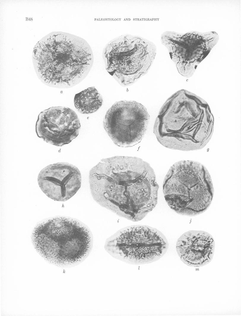
B~ PALEONTOLOGY AND STRATIGRAPHY

c

h

J

k rn

SCOTT AND DOHER B49

Middle Old Red Sandstone, has been identified tenta­tively by McGregor and Owens (1966) from the Lower a.nd Middle Devonian of Canada. It is repre­sented in the Nation River Formation by an unde­scribed species (fig. 3k).

Despite these and other similarities, the Nation River Formation apparently is not as old as Middle Devonian, because it contains genera not known to range below the Upper Devonian. Vigran ( 1964) points out that the genus Foveosporites Balme has not been reported from beds definitely older than Late Devonian. Diaphanospora Balme and Hassell, de­scribed from the Upper Devonian of Australia, and not known from below the Upper Devonian in Canada (McGregor and Owens, 1966) , is present in the Nation River Formation (fig. 3b). Richardson (1965) re­ports that monolete spores, represented in the Nation River Formation (fig. 3l) and in the Upper Devonian of Canada (McGregor and Owens, 1966) by Archaeo-7Je?~isaccus, have been found only once in the Middle Devonian (Russia) but are known from the Upper Devonian of Russia, North America, and Australia.

The original determination of David White (in Mertie, 1930) for the age of the Nation River Forma­tion is borne out by this preliminary examination of plant spores from its upper beds. We attempted to obtain for palynological examination the specimens

FIGUUE 3.-Spores from the Nation River Formation, east­central Alaska. All specimens X 500. Numbers are USGS paleobotany locality and slide numbers.

a. Camptozonotriletes sp. D1940A, slide 20. b. Diaphanospora sp. D1940A, slide 21. c. Samarisporites triangulatus Allen. D1940A, slide 21. d. Lophozonotriletes sp. D1940C, slide 20. e. cf. Convol1ttispora mimerensis (Vigran) Allen. D1940C,

slide 20. f. Foveosporites pertusus Vigran. D1940A, slide 20. g. Calamospora sp. D1940C, slide 20. h. Leiotriletes sp. D 1940C, slide 20. i. Leiozonotriletes sp. D1940C, slide 20. j. ?Ret1tsotriletes sp. D1940A;. slide 27. k. Corystisporites sp. D1940v, slide 20. l. Archaeoperisaccus, cf. A. timanicus Pashkevich. D1940A,

slide 20. m. Raistrickia sp. D1940A, slide 26.

White studied, but they have been discarded (S. H. Mamay, oral commun., 1966). Because the Nation River plant microfossil assemblage from the type area of the formation is in striking contrast to well-known assemblages from the late Paleozoic, a Pennsylvanian or Permian age for the Nation River Formation is precluded.

REFERENCES

Allen, K. C., 1965, Lower and Middle Devonian spores of north and central Vestspitsbergen: Palaeontology, v. 8, p. 687-748.

Balme, B. E., and Hassell, C. W., 1962, Upper Devonian spo·res . from the Canning Basin, Western Australia: Micropaleon­tology, v. 8, p. 1-28.

Brabb, E. E., and Churkin, Michael, Jr., 1964, Preliminary geo­logic map of the Charley River quadrangle (1: 250,000), east-central Alaska: U.S. Geol. Survey open-file report, 1 p.

Brooks, A. H., and Kindle, E. M., 1908, Paleozoic and associated rocks of the Upper Yukon, Alaska : Geol. Soc. America Bull., v. 19, p. 255--314.

Chm·kin, Michael, Jr., and Brabb, E. E .. 1965, Ordovician, Silu­rian, and Devonian biostratigraphy of east-central Alaska: Am. Assoc. Petroleum Geologists Bull., v. 49, p. 172-185.

T.Jaudon, L. R., Hartwig, A. E., Morgridge, D. L., and Omernik, J. B., 1966, Middle and Late Paleozoic stratigraphy, Alaska­Yukon border area between Yukon and Por~upine Rivers: Am. Assoc. Petroleum Geologists Bull., v. 50, p. 1868-1889.

McGregor, D. C., and Owens, B., 1966, Devonian spores of eastern and northern Canada : Canada Geol. Survey Paper 66-30, p. 1-66.

Mertie, J. B., 1930, Geology of the Eagle-Circle district, Alaska: U.S. Geol. ~urvey Bull. 816, p. 1-168.

Playford, Geoffrey, 1962, Lower Carboniferous microfloras of Spitsbergen: Palaeontology, v. 5, p. 619-678.

-- 1963, Miospores from the Mississippian Horton Group, eastern Canada: Canada Geol. Survey Bull. 107, p. 1-47.

Richardson, J. B., 1962, Spores with bifurcate processes from the Middle Old Red Sandstone of Scotland: Palaeontology, v. 5, p. 171-193.

-- 1965, Middle Old Red Sandstone spore assemblages from the Orcadian basin, north-east Scotl~d : Palaeontology. Y. 7, p. 559-605 ..

Vigran, .J. 0., 1964, Spores from Devonian deposits, Mimerdalen, Spitsbergen : Norsk Polarinstitutt, Skr. no. 132, 32 p.

Winslow, M. R., 1.962, Plant spores and other microfossils from Upper Devonian and Lower Mississippian rocks of Ohio : U.S. Geol. ~urvey Prof. Paper 364, 93 p.

GEOLOGICAL SURVEY RESEARCH 1967

TERTIARY STRATIGRAPHY AND GEOHYDROLOGY IN SOUTHWESTERN GEORGIA

By C. W. SEVER and S. M. HERRICK, Tifton, Ga., Atlanta, Ga.

Prepared in cooperation with the city of Oairo, Ga.,

and the Georgia Department of Mines, Mining, and Geology

Abstract.-The section of Oligocene rocks penetrated in the drilling of a test well at Cairo, Ga., is believed from foramini­feral evidence to include beds equivalent to the Marianna Limestone, a formation not known previously to occur in Georgia. Recognition of the Marianna necessitates assignment of some of the overlying beds, formerly considered to be part of the Ocala Limestone of late .Eocene age, to the Byram Formation of Oligocene age. The Byram, not the Ocala, probably is the source of the inferior water previously thought to be contained by the Ocala in southwestern Georgia.

, · Sediments representing the middle and upper Oligo­cene section as known in the southeastern part of the Atlantic Coastal Plain were discovered in the drilling of a test. well in southwestern Georgia. The test well ( GGS 962) drilled by the U.S. Geological Survey at Oairo, Ga., (fig. 1) penetrated rocks of Oligocene age from :a depth of 471 feet to 965 feet, where it bottomed in sediments belonging to the Marianna Limestone of middle Oligocene age. The Oligocene section pene­trated by this well includes a thickness of 494 feet

\ l )

84° 82°

GEORGIA

32°~1~--------+------------------+--------~r f

j\ <I

I ( GRADY \ COUNTY

-\ Well~tairo

COFFEE Well <LcOUNTY

) -l , 0 ' ~ Douglas L-~-J

'----Ll~ I=~~=-----\_:

0 50 100

-....

150 MILES

FIGURE 1.-Location of wells in Coffee and Grady Counties, Ga.

(fig. 2) which compares favorably with that previ­ously described by Applin (1960, p. B208) from a well ( GGS 509) 1 in Coffee County, Ga. In that well a thickness of approximately 635 feet was assigned to the ~ate Oligocene, or post-Marianna part of the Oli­gocene section, as now recognized in Georgia.

S'T!RATIGRAPHY AN,D PALEONTOLOGY

In the Cairo test well the Suwannee Limestone of late Oligocene age occupies the 24-foot interval 471 -495 feet. The sediments composing this part of the section are typically Suwannee, consisting of hard to soft yellowish-gray much calcitized crystalline fossili­ferous limestone. Calcium carbonate makes up about 97 percent of the rock. The Foraminifera Pararotalia 1nexicana (Nuttall) var., .Asterigerina subacuta Cush­man, .A. alabamensis Cushman and MeG lamery, and Quinqueloculfna byramensis Cushman are pvominent in this interval and place this part of the section in the Suwannee.

The Byram Formation, of middle Oligocene age, occupies the interval 459 - 673 feet. These sediments consist predominantly of yellowish-brown dense clayey finely crystalline dolomite. They are similar to the Byram described by Puri and Vern on ( 1964, p. 102) where it crops out along St_ate Highway 71 in Jackson County, Fla. Clay was not observed in un­treated cuttings from the Byram at Cairo~ but when the dolomite is dissolved in hydrochloric acid the residue is a green clay. The clay appears to occur within the rhombohedrons of dolomite instead of be­tween them. Probably owing to their having been dolomitized, the strata assigned to the Byram in the Oairo test well yielded no identifiruble fossils.

1 Carpenter Oil Co., C. T. Thurman No. 2, Coffee County, Ga.

U.S. GEOL. SURVEY PROF. PAPER 575-B, PAGES B50-B53

B50

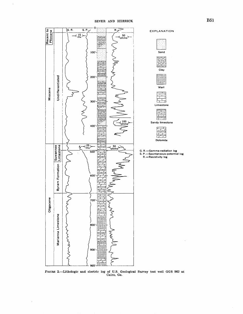
Q) c:: Q) u .!2 ~

Q) c:: Q) u 0

.!!.0 0

"0 Q) ..... ro

:;::; c:: Q) .... Q)

; "0 c::

:::::> '

E ro .... >. m

Q) c:: 0 ..... C/) Q)

E :::; ro c:: c:: ro 'i: ro ~

SEVER AND HERRICK

EXPLANATION

Sand

~ ~

Clay

·Marl

Limestone

Sandy limestone

Dolomite

G. R.-Gamma-radiation log S. P.-Spontaneous-potential log

R.-Resistivity log

FIGURE 2.-Lithologic and electric log of U.S. Geological Survey test well GGS 962 at Cairo, Ga.

B51

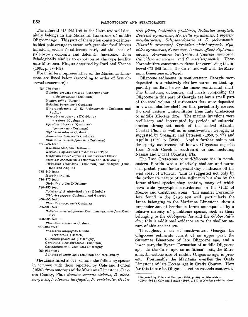
B52 PALEONTOLOGY AND STRATIGRAPHY

The interval 673-965 feet in the Cairo test well defi­nitely belongs in the Marianna Limestone of middle Oligocene age. This part of the section consists of inter­bedded pale-orange to cream soft granular fossiliferous limestone, cream fossiliferous marl, and thin beds of pale-brown dolomite and dolomitic limestone. It is lithologically similar 'to exposures at the type locality near Marianna, Fla., as described by Puri and Vernon (1964, p. 98-102).

Foraminifera representative of the Marianna Lime­stone are listed below (according to order of first ob­served occurrence) :

725-730 feet : Robu.ltts arcuato-striatus ( Hantken) var.

vicks buruensis (Cushman) Nonion affine (Reuss) Bolivina byramensis Cushman Ellipsonodosari.a cf. E. jacksonensis (Cushman and

Applin) Discorbis araucana (D'Orbigny)

assulata (Cushman) Eponides adventts (Cushman)

byramensis (Cushman) Siphonina advena Cushman Anorrialina bilateralis Cushman Oibicidina mississippiensis (Cushman)

730-735 feet: Bulimina sculptilis Cushman Reussella byramensis Cushman and Todd Uvigerina vicksburgensis Cushman and Ellisor Oibicides choctawensis Cushman and McGlamery Oibicidina americana (Cushman) var. antiqua ( Cush-

man and Applin) 735-7 40 feet :

M arginulina sp. 770-775 feet :

Globulina gibba D'Orbigny 780-785 feet :

Robulus cf. R. alato-limbatus (Gumbel) O~bicidps pippeni Cushman and Garrett

850-855 feet : Planulina cocoaensis Cushman

925-930 feet : Bolivina mississippiensis Cushman var. costitera Cush­

man 930-935 feet :

Planulina mea:icana Cushman 940-945 feet :

Nodosaria latejugata Gumbel vertebralis (Batsch)

Gttttttlina problema (D'Orbigny) Gyroi(lina vicksburuens·is (Cushman) Oassidttlina cf. 0. laeviuata D'Orbigny

960-965 feet : Bolivina choctawensis Cushman and McGlamery

The fauna listed above contains the following species in common with those reported by Cole and Ponton ( 1930) from outcrops of the Marianna Limestone, Jack­son County, Fla.: Robulus arcuato-striatus, R. vioks­burgensis, Nodosaria latejugata, N. vertebralis, Globu-

lina gibba, Guttulina problema, Bulimina soulptilis, Bolivina byramensis, Reussella byramensis, Uvigerina vioksburgensis, Ellipsonodosaria cf. E. jaoksonensis, Disoorbis arauoana/ Gyroidina vioksburgensis, Epo­nides byrarn~ensis, E. advenus, Nonion affine,3 Siphonina advena, An01nalina bilateralis, Planulina nwwioana, Oibioidina a'merioana, and 0. 1nississippiensis. These Foraminifera constitute evidence for correlating the in­terval 673-965 feet in the Cairo test well with the Mari­anna Limestone of Florida.

Oligocene sediments in southwestern Georgia were deposited in a relatively shallow warm sea that ap­parently oscillated over the inner continental shelf. The limestones, dolomites, and marls composing the Oligocene in this part of Georgia are but a small part of the total volume of carbonates that were deposited in a warm shallow shelf sea thrut periodically covered the southeastern United States from Late Cretaceous to middle Miocene time. The marine invasions were oscillatory and interrupted by periods of subaerial erosion throughout much of the central Atlantic Coastal Plain as well as in southwestern Georgia, as suggested by Spangler and Peterson ( 1950, p. 97) and Applin (1960, p. B208). Applin further points out the spotty occurrences of known Oligocene deposits from North Carolina southward to and including Nassau and Duval Counties, Fla.

The Late Cretaceous to mid-Miocene sea in north­eastern Florida was a relatively shallow and warm one, probably similar to present-day conditions off the west coast. of Florida. This is suggested not only by the carbonate nruture of the sediments but also by the foraminiferal species they contain, many of which have wide geographic distribution in the Gulf of Mexico and Caribbean areas. The smaller Foramini­fera found in the Cairo test well, particularly the fauna belonging to the Marianna Limestone, show a preponderance of benthonic forms accompanied by a relative scarcity of planktonic species, such as those belonging to the Globigerinidae and the Globorotalii­dae; this is :additional evidence as to the shallow na­ture of this ancient sea.

Throughout much of southwestern Georgia the Oligocene sediments consist of an upper part, the Suwannee Limestone of late Oligocene age, and a lower part, the Byram Formation of middle Oligocene age. In the Cairo age, an additional unit, the Mari­anna Lin1estone also of middle Oligocene age, is pres­ent. Presumably the Marianna overlies the Ocala Limestone of late Eocene age in Grady County. How far this tripartite Oligocene section extends southwest-

2 Reported by Cole and Ponton (1930, p. 40) as Discorbis sp. 3 Identified by Cole and Ponton (1930, p. 37) as Nonion umbilicatulum.

SEVER AND HERRICK B53

ward as well as northeastward (toward Coffee County) from the Cairo area remains to be deter­mined.

QUALITY -OF-WATER CONDITIONS

Ground-water ·studies have indicated that the Su­wannee and Ocala Limestones together yield nearly all of the wruter pumped by the municipal and in­dustrial wells that tap the principal artesian aquifer beneath southwestern Georgia. Some of the water, particularly that in the Cairo area, is known to be extremely hard and to contain concentrations of sul­fate, iron, fluoride, and dissolved solids exceeding to a degree the recommended limits of the U.S. Public I-Iealth Service (1962).

Prior to the drilling of the Cairo test well the poor­quality ground water was thought to occur within the Ocala Limestone. However, geologic and water­quality studies in the Cairo test well plus reexamina­tion of other wells in Grady and neighboring counties hn.ve shown that the inferior water actually is derived from the Byram Formation. The poor quality of water is attributed to the dolomitic character of the r.ocks in the Byram, a part of the geologic section that previously had been placed by Herrick ( 1961, p. 398) in the upper part of the Ocala. By stopping wells

short of the deeper lying Byram Formation and limit­ing pumping to the Suwannee Limestone, or upper part of the Oligocene, the problem of inferior water could be avoided in the Cairo area. If m.ore water is needed than can be obtained from the Suwannee and if additional water supplies are sought ·by drilling to the presumably much 1nore deeply buried Ocala Lime­stone, the Byram Formation should be cased out 1n order to eliminate pumping inferior water from it.

REFERENCES

Applin, E. R., 1960, A tropical sea in central Georgia in late Oligocene time: U.S. Geol. Survey Prof. Paper 400-B, p. B207-B209, 2 figs.

Cole, W. S., and Ponton, G. M., 1930, The Foramlnifera of the Marianna Limestone of Florida : Florida Geol. Survey Bull. 5, p. 19-69, pls. 5-11.

Herri-ck, S. M., 1961, 'Vell log~s of the Coastal Plain of Georgia: Georgia Geol. Survey Bull. 70, 461 p., 1 fig.

Puri, H. S., and Vernon, R. 0., 1964, Summary of the geology of Florida and a guidebook to the classic exposures : Florida Geol. Survey Spec. Rept. 5 (revised), 292 p., 37 figs., 11 pls.

Spangler, W. B., and Peterson, J. J., 1950, Geology of Atlantic Coastal Plain in New .Jersey, Delaware, Maryland, and Virginia: Am. Assoc. Petroleum Geologists Bull., v. 34, no. 1, p. 1-100.

U.S. Department of Health, Education, and Welfare, 1962, Pub­lic Health Service drinking water standards: Public Health Service Pub. 956, 61 p.

GEOLOGICAL SURVEY RESEARCH 1967

FUSTISPOLLENITES, A NEW LATE CRETACEOUS GENUS FROM KENTUCKY

By ROBERT H. TSCHUDY and HELEN M. PAKISER, Denver, Colo.

Work done in oooperation with the Kentuoky GeoZogioaZ Survey

A.bstract.-Fustispollenites. a new pollen genus from the Upper Cretaceous McNairy Formation of Kentucky, is de­scribed and may have biostratigraphic value. It has distinc­tive morphologic characteristics, including prominent apical and subequatorial clavae; comparisons are made with other genera sharing some of these characteristics.

During investigati.ons of plant microfossils from the Mississippi embayment region, a rare, morphologi­cally bizarre angiosperm pollen species was found. It was recovered from a sample of dark-gray clayey silt­stone from the MeN airy Formation of Late Creta­ceous age. .The sample is from an outcr,op 1.35 miles northeast of Faxon School, Kentucky coordinates 1,289,050-135,150 (Carter coordinates 26-C-16), Rico quadrangle, Calloway County, Ky. The sample has been assigned USGS paleobotanical locality No. D3000. T~e pollen is c~ara~terized by 5 colpi separated by

5 ridges, each ridge bearing two prominent sub­equatorial projections or clavae, and two polar clavae. This morphologically unusual pollen resembles in some aspects the genera Senegalosporites Jardine and Magloire, 1963 (pl. IV, fig. 8; pl. V, fig. 1), Elatero­colpites Jardine and Magloire 1963 (pl. IV, figs. 6, 7), and the species Steevesipollenites binodosus Stover 1964 (pl. 2, figs 7-9), all Upper Cretaceous forms from northwest Africa.

The spore genus Senegalosporites and the ephedroid pollen species Steevesipollenites binodosus both possess prominent polar nodes or clavae, but do not possess colpi. The pollen genus Elaterocolpites, perhaps clo~st morphologically to Fustispollenites, possesses colp1 ·and 10 subequatorial projections or outgrowths of the exine, but no polar clavae.

Oareful comparison reveals th3!t resemblance to the above forms is only superficial and that this distinc­tive pollen merits description as a new genus and species. Samples from most of the Upper Cretaceous and lower Tertiary formations of the Mississippi em-

bayment have been examined for fossil pollen con­tent; the genus Fustispollenites has been observed only in the MeN airy Formation. Although rare, its distinctive form makes it a potentially very useful marker fossil in the Late Cretaceous of the Mississippi embayment region.

SYSTEMATIC DESCRIPTIONS

All photographed specimens of the new genus and species described herein are on slides deposited in the U.S. National Museum, Washington, D.C. All illus­trated specimens are within black-ink circles marked directly on the slides; they may also be located on the slides by the mechanical-stage coordinates given in the explaru1tion of figure 1 of this paper._ In order that others may convert their mechanical-stage readings to those recorded for our specimens, our coordinates for the center point of a 1 x 3-inch standard microscope slide :are 108.0 and 12.3 mm. The method of accu­rately locating the center of a standard microscope slide is described by Tschudy (1966, p. D78).

Color photographs of the new genus and species described in this paper are available from the U.S. Geological Survey laboratory, Denver, Colo., on a limited loan basis.

EXPLANATION OF FIGURE 1

a-d Holotype (Slide T3), coordinates 86.3X 14.2 mm. USNM 42633. a-c, taken at different focal planes to show details of colpi, clavae (cl), and surface ornamentation. d, taken with a Wratten-H filter to show detail of colpus (cp).

e-f Para type (Slide T1), coord. 104.1 X 6.3 mm. USNM 42634. g. (Slide T8) coord. 83.6 X 14.5 mm. USNM 42635. One

clava has been broken out (upper right side of photo­graph).

h. (Slide T7) coord. 94.3X20;2 mm. USNM 42636. Note colpus, and vesicles at base of apical clava (acl.)

i-k. (Slide T12) coord. 86.6X3.9 mm. USNM 42637. Polar views, showing lobed outline and wall thickness. k, t~ken with a Wratten-H filter, shows the apical termina~ tlon of a colpus (cp) and the granulate ornamantation of the outer wall.

U.S. GEOL. SURVEY PROF. PAPER 575-B, PAGES B54-B56

B54

TSCHUDY AND PAKISER B55

e f g h

.•

J k

FIGURE 1.- PustispoUenites conspicmts. USGS paleobot. loc. D3000. X 1,000.

B56 PALEONTOLOGY AND STRATIGRAPHY

Genus Fustispollenites n. gen.

Type species.-Fustispollenites conspicuus n. sp. Diagnosis.-Pentacolpate, ellipsoidal to fusiform

pollen with 5 meridional ridges separa;ting colpi. Exine two layered, the outer layer bearing 10 sub­equatorial clavae and two polar clavae. The distinc­tive ornamentation suggests the latin term "fustis", a knobbed stick or club.

Fustispollenites conspicuus n. sp. Figure 1, a-k

Holotype: USNM 42633, slide D3000 (T3), coordi­nates 86.3 X 14.2, fig. 1, a-d. Size 43 microns X 28 microns exclusive of clavae.

Paratype: USNM 42634, slide D3000 (T1), coordi­nates 104.1 X 6.3, fig. 1, e, f. Size 38 microns X 24 microns exclusive of cia vae.

Description (18 specimens) .-These pentacolpate pollen grains are elongate, cylindrical to spindle shaped, and symmetrical around the longitudinal axis. In polar view the outline is five lobed, the colpi lying in the grooves between the lobes. The colpi extend about three-quarters of the distance to the poles. They are open, possess rounded ends, and are dilated at the equator, giving the appearance of a pore. The inner­wall layer (endexine) is uniformly slightly more than 2J.L thick except at the colpi, where it is absent. The outer-wall layer (ektexine) is less than 1J.L thick and possesses a finely granulate surface.

On each of the lobes of the outer wall, midway between the colpi, two clavae are inserted. The clavae are solid, smooth, and slightly enlarged at their ends. The subequatorial cia vae range from 5 to 7 J.L in length, and average 3.1J.L in diameter at their midpoints and 4.3J.L in diameter at their ends. Two somewhat larger cia vae are inserted on the two poles. They are 7 to 9J.L in length and average 5J.L in diameter at their midpoints and 6.4J.L in diameter at their ends.

The size of this pollen grain, excluding the cia vae, ranges from 37 to 43J.L in length; and from 18 to 28J.L in diameter.

Discussion.-The clavae are inserted into the outer layer of the wall, rather than being extensions of the wall. This is shown on figure 1, g, where one of the clavae has been clearly broken out. The granulate surface texture of the outer-wall layer is shown on d and k, taken with a Wratten-H filter.

Occurrence.-McNairy Formation of Kentucky. Age.-Late Cretaceous, Maestrichtian. Oomparisons.-Fustispollenites conspicwus differs

from other genera possessing prominent polar or lat­eral knobs or cl:a vae as shown in table 1.

TABLE I.-Comparison of Fustispollenites conspicuus with other genera

Fustis- Elatero- Senegalo- Steevesi-sporites poUenites

binodosus pollenites . colpites

conspicuus

Polar knobs or clavae____ + 10 subequatorial clavae +

or extensions of exine.

-------- + + +

Colpi__ _________________ + + Equatorial clavae as _ _ _ _ _ _ _ _ +

extensions of outer membrane.

This distinctive, easily recognized angiospermo1113 fossil pollen shows no direct affinity with any known palynomorph.

REFERENCES

Jardine, Serge, and Magloire, L., 1963, Palynologie et Strati­graphie du Cretace des Bassins du Senegal, et de Cote d'Ivoire: Colloque International de Micropaleontologie, Dakar, 6-11 Mai, p. 187-245.

Stover, L. E., 1964, Cretaceous ephedroid pollen from West Africa: Micropaleontology, v. 10, no. 2, p. 145-156.

Tschudy, R. H., 1966, Associated megaspores and microspores of the Cretaceous genus Ariadnaesporites Potonie 1956, emend, in Geological Survey Research 1966: U.S. Geol. Survey Prof. Paper 55Q-D, p. D76-D82.

GEOLOGICAL SURVEY RESEARCH 1967

ORIENTATION OF CARBONATE CONCRETIONS

IN THE UPPER DEVONIAN OF NEW YORK

By GEORGE W. COLTON, Beltsville, Md.

A.bstract.-Argillaceous limestone concretions are abundant in the lower Upper Devonian marine sequence in New York. Typically they are elongate in plan view, and their long axes are preferentially oriented to the northeast. The alinement of the concretions is probably parallel to the primary deposi­tional fabric of the enclosing rock. In turn, the fabric was proba,bly controlled by, and oriented parallel to, marine cur­rents.

The lower Upper Devonian rocks in the western half of New York consist of evenly interstratified black shale, gray shale and mudrock, siltstone, and sandstone. Regional stratig~aphic studies (fig. 1) in­dicate that they accumulated in a marine basin whose axis and eastern shoreline trended approximately northeast-southwest. The Genesee, Sonyea, West Falls, Java,, and Perrysburg Forma)tions, which make up .the lower Upper Devonian sequence, thicken to the east and southeast across most of the area. As the formations thicken, members composed largely of silt­stone and sandstone increase in number and in thick­ness. Conversely, the percentage of gray shale and mudrock :and of black shale in each formation de­creases to the east and southeast.

Calcareous concretions occur in large numbers in all the formations. They are most abundant in mem­bers composed largely of shale and mudrock, and consequently occur in greatest abundance in the west­ern part of the area, where shale and mudrock make up the bulk of the formations. The directional prop­erties of concretions were studied at 27 localities in an area 105 miles wide, extending from Lake Erie east­ward to Seneca Lake. Data were collected in the following counties: Chautauqua, Cattaraugus, Erie, "ryoming, Livingston, Ontario, Yates, Steuben, Schuyler, and Tompkins.

DESCRIPTIONS OF CON.CRETIONS

"Concretion" is a general term used here to include three forms of accretionary structures : nodules, true

concretions, and septaria or septarian nodules (Petti­john, 1949, p. 149-154). All three forms are com­posed largely of clay, quartz, and calcium carbonate. Pyrite or marcasite, and barite are the most common accessory minerals. On the basis of field observations in New York, nodules in general are the smallest con­cretionary structures. They are commonly irregular in shape, have a warty or pustulose surface, and do not appear to be internally laminated. In many places, nodules occur in such great numbers along bed­ding planes that they locaJly coalesce to form lumpy lenses and lenticular beds of argillaceous limestone. True concretions are commonly larger, more symmet­rical in shape, and have smoother surfaces than nod­ules, and, as a rule, contain an internal lamination that is parallel to that of the surrounding rocks. In most places, true concretions are widely spaced along the bedding plane in which they occur and coalesce less commonly than nodules. Septaria are charac­terized by fractures containing coarsely crystalline calcite and smaller amounts of pyrite, barite, siderite, and other mine~als. The fractures have a tendency to radiate irregularly outward from near the center of the concretion and to become narrower or to ter- · minate near its surface. Concentric banding, due largely to variations in the am.ounts of finely crys­talline pyrite, calcite, and argillaceous material, is pro­nounced in many septaria. In size, shape, surface texture, and in their arrangement along . bedding planes, septaria are similar to true concretions. The long axes of concretions range from a fraction of an inch to about 15 feet in length, and invariably lie along the bedding plane. With few exceptions, the short axis of the concretion is perpendicular to bed­ding. Small fragments of pl~nts, pteropods, thin­shelled gastropods, and pelecypods occur in many true concretions and septaria and in some nodules. Most fossils in the concretions are undeformed by compac-

U.S. GEOL. SURVEY PROF. PAPER 575-B, PAGES B57-B59

B57

B58 SEDIMENTATION

43 Syracuse~

42 I ---------------------------0 10 20 30 40 MILES

FIGURE 1.-Map of report area in western New York, S'howing localities (dots) where data were collected.

tion, whereas fossils in the surrounding shale or mud­rock are highly compressed.

Of the concretions observed, approximately two­thirds are noticeably elongate in plan view, and the remainder are for the most part equant or highly ir­regular in plan view (fig. 2). The degree of elonga­tion varies from slightly ellipsoidal in some specimens to rodlike or nearly cylindrical in others.

ORIENTATION OF CONCRETIONS

The orientations of the long axes of 64 7 concretions are compiled in figure 3. It is apparent that the long

Elongate

Irregular and equant

FIGURE 2.-Typical shapes of concretions.

axes are preferentially grouped about a northeast axis and that the mean trend is N. 55° E. To determine if a relationship exists between the orientation of con­cretions and the environment of deposition of the en­closing rocks, the concretions were divided into two groups. One group includes concretions in the area west of the Genesee River, where the rock sequence is composed largely of shale and mudrock. These rocks accumulated in the marine basin far west ·of the shoreline. The other group includes concretions in the area east of the Genesee River, where siltstone -and sandstone constitute an appreciable part of the sequence. The rocks in this area accumulated closer to the shoreline, presumably in shallower water under the influence of stronger currents.

The orientation of the long axes of the concretions in the two areas is compared in figure 3; The fact that the primary peaks of both groups coincide sug­gests that the principal orienting force or phenomen-a was constant in direction regardless of geographic location and environment. A secondary peak in the lower line (in the northwest quadrant) suggests an­other orienting force or the same force operating in a different direction or manner in the western are:a. This secondary maximum is absent among the elon­gate concretions measured in the east. Figure 3 also shows that the orientation of concretions in the west is less pronounced than that of concretions in the east.

An earlier investigation of other elongate sedimen­tary and organic structures in the same rock sequence (Colton, 1967) showed that specimens of F~woides grophica Vanuxem and of plant fragments in shale

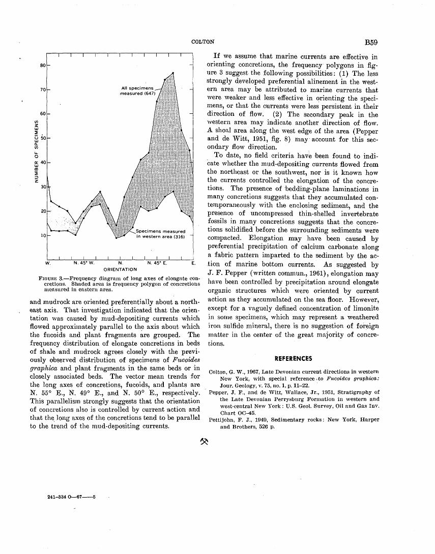
COLTON B59

(/')

z LI.J :::?! u 5o LI.J Q.. (/')

Lo.. 0 0:: 40 LI.J CD :::?! ::> z

w. N. 45" W. N.

Specimens measured in western area (316)

N. 45• E.

ORIENTATION E.

FioUim 3.-Frequency diagram of long axes of elongate con­cretions. Shaded area is frequency polygon of concretions measured in eastern urea.

and mudrock are oriented preferentially about a north­east axis. That investigation indicated that the orien­tation wns caused by mud-depositing currents which flowed approximately parallel to th~ axis about which the fucoids and plnnt fragments are grouped. The frequency distribution of elongate concretions in beds of shale and mudrock agrees closely with the previ­ously observed distribution of specimens of Fuooides g'raphica and plant frngments in the sa-me beds or in closely associated beds. The vector menu trends for the long axes of concretions, fucoids, and plants nre N. 55° E., N. 49° E., and N. 50° E., respectively. This parallelism strongly suggests that the orientntion of concretions also is controlled by current action and thnt the. long axes of the concretions tend to be pnrallel to the trend of the mud-depositing currents.

241-834 0-67--5

If we assume that marine currents are effective in orienting concretions, the frequency· polygons in fig­ure 3 suggest the following possibilities : ( 1) The less strongly developed preferential alinement in the west­ern area may be attributed to marine currents that were weaker and less effective in orienting the speci­mens, or that the currents were less persistent in their direction of flow. ( 2) The secondnry penk in the western area may indicate another direction of flow. A shoal area along the west edge .of the area (Pepper and de Witt, 1951, fig. 8) may· account for this sec­ondary flow direction.

To date, no field criteri'a ha~~ been found to indi­cate whether the mud-depositing currents flowed from the northeast or the southwest, nor is it known how the currents controlled the elongation of the concre­tions. The presence of 'bedding-plane laminations in many concretions suggests that they accumulated con­temporaneously with the enclosing sediment, and the presence of uncompressed thin-shelled invertebrate fossils in many concretions suggests that the concre­tions solidified before the surrounding sediments were compacted. Elongation may have been caused by preferential precipitntion of calcium carbonate along a fabric pattern imparted to the sediment by the ac­tion of marine bottom currents. As suggested by J. F. Pepper (written commun., 1961), elongation may have been controlled by precipitation around elongate organic structures which were oriented by current action as they accumulated on the sea floor. However, except for a vaguely defined concentration of limonite in some specimens, which may represent a weathered iron sulfide mineral, there is no suggestion of for~ign matter in the center of the great majority of concre­tions.

REFERENCES

Colton, G. W., 1967, Late Devonian current directions in western New York, with special reference .to F1tCoides graphica: Jour. GeOlogy, v. 75, no. 1, p. 11-22.

Pepper, J. F., and de Witt, 'Vullace, Jr., 1951, Stratigraphy of the Late Devonian Perrysburg Formation in western and west-central New York: U.S. Geol. Survey, Oil and Gas Inv. Chart 00-45.

Pettijohn, F. J., 1949, Sedimentary rocks: New York, Harper and Brothers, 526 p.

GEOLOGICAL SURVEY RESEARCH 1967

A STATISTICAL MODEL OF SEDIMENT TRANSPORT

By W. j. CONOVER 1 and N. C. MAT ALAS, Manhattan, Kans., Washington, D.C.

Ab8tract.:-A statistical model is constructed to simulate the behavior of sediment particles in flowing water in order to obtain a theoretical shape for the suspended-sediment concen­tration profile. The model yields the same shape or profile as does the classical deterministic model based on the linear­diffusion hypothesis.

Know ledge of the theoretical shapes of the velocity profile and sediment-concentration profile helps in de­termining the total suspended-sediment load beinO' car-

• 0

r1ed by a stream. The classical profile of suspended-sediment concentration given by Rouse ( 1950) has long been used for this purpose. This pa·per shows that for suspended particles of uniform fall ~elocity, the same theoretical shape of profile can be computed by a statistical. model as by the differential equation model used in Rouse.

On the basis of a statistical model of turbulence, Matalas and Conover (1965) derived the vertical­velocity profile for two-dimensional uniform flow in open channels. The model itself was based on a prob­ability law that .governed the transfer of momentum of the fluid, taking into account momentum loss due to friction at the streambed and to fluid viscosity. Some simple modifications of this model alter its interpreta­tion from that of the transfer of momentum to that of the transfer of mass. With these modifications, the model may be used in studies of sediment transport. In the following paragraphs, the main features of the mass-transfer model and the application of this model to derive the vertical sediment-concentration profile are presented.

Flow is assumed to be confined to a two-dimensional channel of depth D and unit width, with discharge restricted to the downstream direction. The channel of flow is considered to be subdivided into n different levels, Bt, ranging from B1 just below the surface to Bn resting on the streambed. These levels resemble layers of unit width and depth W=Dfn. As the model represents a situation which changes continuously in time, it will be convenient to denote "level i at time

1 Kansas State University.

t" by Bt(t). For the present, time will be considered in terms of discrete intervals of duration dt. Later, a continuous model is evolved from the discrete model by aHowing dt and W to approach zero.

The transfer of sediment mass from one level to another is assumed to be governed by the following probability law. The mass Mt(t) associated with lev~l B1(t) is transferred to level Bt-I(t+dt), Bt(t+dt), or Bt+l (t+ dt) with probability p, q, or r, respectively, where p+q+r=1, for all values of i except i=1 and i=n. The stream surface and bed are assumed to act as reflecting barriers, so that any mass which attempts to penetrate these barriers is returned to the flow sec­tion in the following manner. The mass M 1 (t) associ­ated with block B1 (t) is transferred to level B1 (t+ dt) or B2(t+dt) with probability (p+q) or r, respectively. And the mass Mn(t) associated with level Bn(t) is trans­ferred to level Bn(t+dt) or Bn_1(t+dt) with probability (r+q) or p, respectively. This probability law holds for the transfer of mass from any time t to time t+ dt and, therefore, the total sediment mass at any time is a constant. The probabilities p, q, and r are referred to as 1-step transition probabilities.

If Pt.1(k) denotes the k-step transition probability for the transfer of mass from Bt(O) to B 1(k·dt), where t=O is an initial time reference point, then

Pt.1(k)=pPt,J+t(k-1)+qPt.1(k-1) +rPt,J-l (k-1); j=2, ... , n-1

Pt,l(k)= (p+q)Pt,t(k-1)+pPt,2(k-1); j=1 (1)

Pt,n(k)=rPi,n-t(k-1) + (q+r)Pt,n(k-1); J=n

The expected value of the sediment mass transferred from Bt(O) to B 1(k · dt), denoted by Mt./k), is equal to Mt(O)Pt, 1(k), and the total expected value of mass con­tributed to B/k·dt) from Bt(O) for all values of i, denoted .by M 1(k), is given by

n

(2)

1=1

U.S. GEOL. SURVEY PROF. PAPER 575-B, PAGES B6G-B61

B60

CONOVER AND MATALAS B61

To solve for M 1(k) in the limiting case where n~oo and k~oo, the following properties of the probability model must be considered: 1. The transition probabilities have a long run distri­

bution so that in the limit as k~oo, Pt,1 (k)~7r11 where 1r1 is some constant independent of i (Par­zen, 1962).

2. For a fixed value of D, tJJ goes to zero as n goes to infinity and the ith level approaches the surface for a fixed value of i. Therefore, to consider the mass at a constant depth proportional to D as n~oo, let 1-i/n=m, the proportionate height from the bed.

3. To obtain meaningful results as w~o, !lt must approach zero in such a way that (ll.D) 2/ !lt ap­proaches a constant (Feller, 1957).

4. Because the density of sediment exceeds that of water, p<r. Thus the expected level of a sedi­ment particle starting at level i is i+ (r-p) after a time interval !lt, where (r-p) is the expected fraction of !lD that a sediment particle drops during the time interval !lt.

5. The total expected drop per unit time (r-p)ll.Dj!lt, which equals (r-p)(llD) 2n/Dllt, should approach a constant as tJJ and !lt go to zero for the model to be meaningful. Thus n(r-p) approaches a con­stant. In particular let the constant (3=n(r-p)fr =n(1-p/r), so the above requirement is met. Then p/r is equal to 1-(3/n, which satisfies the condition that pfr~1 as n~oo (Feller, 1957).

With these properties, the mass at level j as k~oo is

(3)

where M denotes the mean value of the mass in the vertical. The values of 1r1 are obtained from the solu­tion of the systems of equations 1 where 1r11 'lrJ+t,'lrJ-t, 7rt, 7rt, 1r2, 'Trn, 'Trn-·l, and 'Trn are substituted for Pt,JCk), Pt,J+t(k-1), Pt,J-•(k-1), Pt,t(k), Pt,.(k-1), Pt,a(k-1), P 1,n(k), Pt,n-1(k-1), and P 1,n(k-1), respectively.

T his solution is given by

1r1= (p/r)n-1[1- (p/r)]/[1- (pfr)n]. (4)

f

In the limit as n~oo ,

lim n7r1={3e~~mf(l-e-~), (5) n.--+m

where m= 1-jfn. Therefore, the sediment-concentra­tion profile is given by

lim nM7r1=Mm=M(3e-tJmj(l-e-~). (6)

The parameter (3 is a function of the fall velocity of the sediment particles and of the intensity of turbu­lence. ·As (3~0, the sediment-concentration profile ap­proaches M. That is, in the limit, the concentration of sediment is a constant, independent of depth. In general, the concentration is a minimum at the stream surface and increases exponentially to a maximum at the streambed. This description of the sediment­concentration profile is essentially the same as that obtained by the use of the differential equation of diffusion (Rouse, 1950). It is of some interest to note that equation 6 leads to

~;';n=-~ Mm, (7)

which has the same form as the differential equation in Rouse (1950). Therefore

(3 w -=-l D E

where W is the fall velocity and E Is the turbulent mixing coefficient.

REFERENCES

Feller, William, 1957, An introduction to probability theory and its applications: New York, John Wiley and Sons, v.1, 249 p.

1\fatalas, N. C., and Conover, W. J., 1965, Derivation of the velocity profile from a statistical model of turbulence : \Vater Resources Research, v. 1, no. 2, p. 235-261.

Parzen, Emanuel, 1962, Stochastic processes : San Francisco, Calif., Holden and Day, 325 p.

Rouse, Hunter, 1950, Engineering hydraulics: New York, John Wiley and Sons, p. 780-799.

GEOLOGICAL SURVEY RESEARCH 1967

NEW OBSERVATIONS ON THE SHEYENNE DELTA OF GLACIAL LAKE AGASSIZ

By CLAUD H. BAKER, JR., Salt Lake City, Utah

Work done in cooperation with the

North Dakota State Water Commission and the North Dakota Geological Survey

A.bstract.-The Sheyenne delta is an extensive deposit of gravel, sand, and silt near the south end of the basin of glacial Lake Agassiz. The deposit has been called both a delta and a body of ice-contact stratified drift, but recent test drilling and field observations indicate that the deposit is a true delta and that the steep slope formerly descri'bed as an ice-contact face is probably a wave-cut "cliff." The. delta is not so ex­tensive as originally believed, and the boundaries have been redefined. The location of dunes on the delta surface with respect to possible sources of sand indicates that prevailing winds probably were from the southwest when the dunes were formed.

In late Pleistocene time, the valley now drained by the Red River of the North was the floor of a large proglaci'al lake. The existence of such a lake was recognized as early as 1823, and the lake was named Lake Agassiz by Warren Upham ( 1880, p. 85) in honor of Jean Louis Agassiz, an early advocate of the gl·acial theory. At its maximum, Lake Agassiz prob­ably extended from northern South Dakota to central Manitoba.

At sever.al points where large valleys enter the Lake Agassiz basin, the mouths of the valleys are marked by extensive bodies of gravel, sand, -and silt, which are believed to be deltas deposited in the former lake by melt-water streams that emptied into it. One of the largest of these deposits is in southeastern North Dakota, ne:ar the southern end of glacial Lake Agassiz. Because it radiates from the point where the present Sheyenne River enters the Lake Agassiz plain, it has been called the Sheyenne delta (fig. 1).

Upham (1895) made the first comprehensive survey of the southern end of Lake Agassiz. Leverett (1913, 1932) generally agreed with Upham's views of the lake basin, but concluded that . the deltas were ice­contact deposits of stratified drift. Although Elson ( 1957) agreed with Leverett on the .origin of the

deltas, Dennis and others (1949, 1950) found subsur­face evidence to support Upham's views. Laird (1964) summarized the existing literature on Lake Agassiz.

This report is based on work done in 1963 and 1964 in connection with a study of the geology and ground­water resources of Richland County, N. Dak. The study was conducted under the cooperative program of the U.S. Geological Survey, the North Dakota State Water Commission, and the North Da~ota Geological Survey.

47

46

~ j

_ _l __ _ LA MOURE j

____ _j ____ _ I

DICKEY I SARGENT

----·-·l_ _____ _i ____ _ SOUTH DAKOTA

0 50 MILES

FIGURE 1.-Location of the Sheyenne delta (diagonal pat­tern) and the Lake Agassiz plain (stippled pattern).

U.S. GEOL. SURVEY PROF. PAPER 575-B, PAGES B62-B68 B62

BAKER B63

Most .of the information reported here about the delta has been obtained by test drilling. Thirty-four test holes were drilled during this study, and 53 test holes were drilled during earlier studies (Dennis and others, 1949, 1950, and unpublished data).

AREAL EXTENT AND TOPOGRAPHY

The Sheyenne delta has an area of about 750 square miles and is roughly deltoid in outline (fig. 1). It is bounded on the west and southwest by the drift prairie :and on the northeast, east, and southeast .by the Lake Agassiz plain. The northeastern edge is a well-defined steep slope, but the southeastern edge merges imperceptibly with the lake plain.

The area of the Sheyenne delta is somewhat less than was mapped originally by Upham (fig. 2). Upham's nrap included in the delta a portion of an ice-marginal channel called the Milnor channel (Baker, 1966) that is somewhat older than Lake Agassiz, an area of glacial till between the Milnor channel and the delta, a part of the lake floor, and a large sandy tract southeast of the delta. Presum­ably, Upham included the area of till in his map of the Sheyenne delta because he believed that the line of the Milnor channel represented the southwestern edge of the delta :and the shoreline of Lake Agassiz. Recent studies by the writer indicate that the highest shoreline of Lake Agassiz is marked by the line of the Herman beach, and that the till southwest of the I-Ierman beach does not appear to have ever been covered by water. The southern area of sand (Lake Agassiz beaches, fig. 2) is a beach complex of the same age as, or slightly younger than, the Sheyenne delta. Erosion of the delta may have furnished part of the sand to the southern beach complex, but the area is not a part of the delta proper. Part of the lake floor. between the delta and the beach complex was apparently included in the delta hy assuming .that 'the eastern edges of the delta and the beach complex were continuous.

The Sheyenne River crosses the north end of the delta in a deeply incised meandering valley. The valley floor is as much as 100 feet below the adjacent delta surface.

A large part of the delta surface is covered by sand dunes. In places, the topography is highly undulat­ing, with local relief as much as 75 feet. Most of the dunes are well stabilized by vegetation, but consid­erable sand movement still occurs whenever the vege­tal cover is bt:oken. The high dunes are bordered on the southwest by a wide band of nearly level sand on the delta; the average elevation of the sand plain is about 1.07 5 feet. The probable significance of the

sand plain will be discussed in a later section of this report (p. B67).

THICKNESS, GRAIN SIZE, AND BEDDING OF SEDIMENTS

The bottom of the delta deposits cannot be distin­guished in drill holes. An advancing delta is built out over its own bottomset beds, as well as over any preexisting lake-floor deposits, and it is nearly im­possible to distinguish between delta bottomset beds and lake silts of similar composition. The thickness of the lake-floor deposits east of the delta averages about 60 feet. In this discussion the thickness of the Sheyenne delta will be taken as the total thickness of sand, silt, and clay-that is, the depth to the glacial till.

The greatest known thickness of the delta is 198 feet (fig. 3) and the average thickness of the eastern half is about 150 feet. West of the Richland-Ransom County boundary the surface of the till beneath the delta slopes sharply upward, and the delta is only a few feet thick near its western edge.

The average grain size of the delta sediments de­creases from west to east (fig. 3) . Near the western margin, where the deposits are only a few feet thick, they consist of very coarse sand and fine gravel ; but near the eastern margin, where the deposits are more than 150 feet thick, they consist of very fine sand and silt. This gradation of average grain size is consistent with the increased distance of tt~ansport across the top of the growing delta.

The average grain size of the sediments also de­creases from top to bottom. The decrease is not marked near the thin western margin of the delta but is quite apparent in the thicker central part. Near the eastern margin, material making up the entire thick­ness of the delta is fine grained, and vertical differ­ences in grain size are difficult to determine. This too, is consistent with the concept of a delta that expanded eastward.

In figure 4, parts of the deposit have been distin­guished as predominantly silt or predominantly sand. The silt is thickest near the eastern margin and wedges out to the west; the sand wedges out to the east. Again, these relationships would be expected in this particular deltaic environment.

Exposures of the bedding in the delta are very scarce. The best exposures found are in the bank of a short gully in the EY2 sec. 15, T. 136 N., R. 51 W., near the northeastern edge of the delta (location 0-1, fig. 3). At this location, the sediment consists of very fine sand, silt, and clay. Here the sand and silt are well stratified, and ripple lamination is the most com-

B64

46°30'

• . 0

."' ...

. 0 •.

. . 0 .. .. .

. 0

~ . • 0

·'

... 0

. 0

. Q .

:> a. :o

0 .. 0 . 0

.,· : . ~

. 0 .. . ~ .

0' ' .

. Q.

'o

0 ...

·. ... . o·

·I>

0

46° .. '<:> ..

. (',.·

· ...

...

·o

. 0.

. . . ·. n

GEOMORPHOLOGY AND PLEISTOCENE GEOLOGY

.,·

0.

. 0.

. . . . c:,'

10 MiLES

. . .,;_. . 0 •

0 .

·o· . ·., .

,, : .·

0 .. · ......

·o.

EXPLANATION

~ ~

Sheyenne delta (this report)

Milnor channel and Lake Agassiz beaches

Lake-floor deposits

Diagonal-line pattern shows extent of Sheyenne delta of Upham (1895, pl. 27)

Glacial till

FIGURE 2.-Relationship of the Sheyenne delta as defined in this report, to the ·area included in the Sheyenne delta of Upham.

46°30'

97°30'

RANSOM COUNTY

SARGENT COUNTY

D . . Coarser than coan;e sand

~ ~

Coarse to medium sand

BAKER

EXPLANATION

D . . .

Medium to fine sand

Finer than fine sand

0 5

--100--­Isopach, showing thickness

of delta deposits Dashed where approximately

located. Interval 20 feet

.o-1 Exposure showing strati­fication of delta deposits

10 MILES

I!..,IOURI~ 3.-'l'otal thiclmess of delta deposits, in feet, and average grain size of the near-surface materials.

B65

B66 GEOMORPHOLOGY AND PLEISTOCENE GEOLOGY

~ Predominantly silt and clay

Predominantly but may include shale bedrock locally in Ransom County

Datum is 800 feet above mean sea level. Outlines of the delta and county boundaries are on the datum plane

Margin of Sheyenne delta

FIGURE 4.-Fence diagram of the Sheyenne delta.

mon form of stratification (fig. 5A) . No stratification is apparent in the clay layers. Some of the sand and silt beds are strongly. contorted on a small scale (fig. 5B), but the causes of this are not known. However, such contortions are common in deltaic and flood-plain deposits.

The delta bedding was exposed temporarily in a roadcut in the NE1,4 sec. 13, T. 136 N., R. 51 W. (loca­tion 0-2, fig. 3). Here, the ripple-laminated sand con­tains thin films and pockets of carbonaceous material (fig. 50). This exposure was destroyed later by road improvements.

PROBAB-LE PROCESS OF FOR'MATION

The Sheyenne delta probably was deposited rather rapidly, during the earliest and highest stages of Lake Agassiz. The Sheyenne River apparently was an ice­m1arginal stream just prior to the formation of Lake Agassiz (Baker, 1966) and probably was diverted into Lake Agassiz soon after the lake was formed. Be- · cause the river was fed primarily by glacial melt water, it must have carried abundant sediment, and

deposition of the delta would have begun as soon as the stream began flowing into the lake.

Most of the surface of the delta is at or near the altitude of the highest (Herman) shoreline of Lake Agassiz. Two slightly lower shorelines (the Tintah and the Norcross) were mapped across the delta by Upham ( 1895), but this author was unable to distin­guish them. The fourth, or Campbell, shoreline is probably represented by the steep slope at the north­eastern edge of the delta.

The steep northeastern edge of the delta was the principal evidence cited by Leverett (1913, 1932) for his belief that the delta was a deposit of ice-contact stratified drift. Leverett ( 1932, p. 127) had very little subsurface data, and he thought that glacial till was only a few feet below the surface near the top of the slope. However, logs of test holes in the area show that the sand, silt, and silty clay are more than 150 feet thick near the northeastern edge of the delta. No other evidences of ice-contact deposition were found during the present study." The slope is at the level of the Campbell shoreline north and south ,of the delta, and this author concludes that the slope is a wave-cut

BAK E R B67

"cliff'' representing the Campbell shoreline of Lake Agassiz.

\iVhen Lake Agassiz began to recede from its high­est (Herman) level, the base level of the Sheyenne River was lowered, and the river entrenched itself into the recently formed delta. The position of the present valley was deterlnined by the position tha,t the river happened to occupy when the lake level was lowered.

SAND DUNES ON TH E DELTA

The sand dunes that cover much of the surface of the delta probably began to form when Lake Agassiz was first lowered to the Campbell level. As the lake kvel declined, the emerging surface of the delta would have been highly susceptible to erosion by wind. The dunes are largest and most numerous near the north­eastern margin of the delta and become smaller and less numerous southwesbYard. Thus, the broad sand plain on the part of the delta southwest of the high

FIGURE 5.-Stratification and small-scale structures in sedi­ments of the Sheyenne delta. A, Stratification in a section exposed in the bank of a gully on the east side of sec. 15, T. 136 N., R. 51 W. (location o-1, fig. 3). B, Small-scale contor­tions in stratified sediments; location same as A. 0, Ripple­laminated delta sand containing films and pockets of car­bonaceous material, exposed in temporary roadcuts in NE1,4 sec. 13, T. 136 N., R. 51 W. (location o-2, fig. 3).

dunes may have been the source area of the dune sand, and, if this were so, the prevai•ling winds would have been from the southwest. Because the dune area con­sists of hummocky topography rather than of discrete well-formed dunes, the orientation of the dunes is of little help in determining wind directions. Further­more, the stratification within the dunes is not exposed well enough to be used as a key to wind direction.

Clayton and others ( 1965, p. 655) have interpreted lineations on the Lake Agassiz plain to mean that prevailing winds were probably from the northwest or wmtheast in late Lake Agassiz time. However, the loca­tion of the dunes \Yith respect to possible source areas of the sand does not support such a hypothesis. The sediments near the lakeward margin of the delta are predominantly si·lt. size, whereas the material in the dunes is largely in the fine-sand range, and there is no nearby source of fine sand to the north, east, or southeast of the delta front. Although the evidence from the Sheyenne delta is hardly conclusive, the

B68 GEOMORPHOLOGY AND PLEISTOCENE GEOLOGY

presence ,of an extensive sand plain southwest of an area of dunes suggests that prevailing winds were from the southwest when the dunes were formed. Possibly the prevailing winds were from the southwest in Oampbell time and shifted to northwest-southeast later.

If the sand plain was the source of the dune sand, the depth to which erosion by the wind lowered the surface of the sand plain would have been controlled by the water table in the delta sediments. Hence the 1,075-foot present elevation of the sand plain may have been the average elevation of. the water table during Campbell time.

SU'M·MARY

In summary, recent studies of the Sheyenne delta lead to the following conclusi'Ons:

1. The form, lithology, and stratification a.Il indi­cate that the Sheyenne de,lta is a true deltaic deposit, as suggested by Upham (1895), rather than a body of ice-contact stratified drift, as postulruted by Lev­erett(1913, 1932). The steep northeastern slope is not an ice-contact face, but a wave-:-cut "cliff" marking a shoreline of Lake Agassiz.

2. Upham's map of the delta included parts of the Lake Agassiz beaches, a pre-Lake AgaJSSiz outwash channel, and adjoining areas of ground moraine and lake floor tluut are not parts of the delta.

3. The locrution of dunes on the delta with respect

to sources of sand indioates that prevailing winds probably were from the southwest when the dunes were formed, and that the average position of the water table at that time may have been at about the 1,075-foot elevation of the sand plain.

REFERENCES

Baker, C. H., Jr., 1966, The Milnor channel, an ice-marginal course of the Sheyenne River, in Geological Survey Re­search 1966: U.S. Geol. Survey Prof. Paper 550-B, p. B77-B79.

Clayton, Lee, Laird, ,V. M., Klassen, R. ,V., and Kupsch, ,V. 0., 1965, Intersecting minor lineations on Lake Agassiz plain: Jour. Geology, v. 73, no. 4, p. 652-656.

Dennis, P. E., Akin, P. D., and Jones, S. L., 1949, Ground water in the ·wyndmere area, Richland County, N. Dak.: North Dakota Ground-,Vater Studies 13, 55 p.

-- 1950, Ground water in the Kindred area, Cass and Rich­land Counties, N. Dale: North Dakota Ground-,Vater Stud­ies 14, 75 p.

Elson, J. A., 1957, Lake Agassiz and the Mankato-Valders: prob­lem: Science, v. 126, no. 3281, p. 999-1002.

Laird, W. M., 1964, The problem of Lake Agassiz: North Dakota Acad. Sci. Proc., v. 18, p. 114-134.

I.~everett, Frank, 1913, Early stages and outlets of Lake Agassiz in relation to the waning ice sheet: North Dakota Agr. Ooll. Survey, 6th Bienn. Rept., p. 18-28.

-- 1932, Quaternary geology of Minnesota and parts of ad­jacent states: U.S. Geol. Survey Prof. Paper 161, 149 p.

Upham, Warren, 1880, Preliminary report on the geology of cen­: tral and western Minnesota: Geol. and Nat. Hist'Ory Survey

of Minnesota, 8th Ann. Rept., p. 70--125. --1895, The glac.ial Lake Agassiz: U.S. Geol. Survey Mon.

25, 658 p.

GEOLOGICAL SURVEY RESEA~RCH 1967

GROSS COMPOSITION OF PLEISTOCENE CLAYS

IN ·sEATTLE, WASHINGTON

By DONAL R. MULLINEAUX, Denver, Colo.

Work done in co_operaUon with the M1tnicipality of Metropolitan Seattle

A.bstract.-Unweathered glaciolacustrine and glaciomarine deposits of relatively uniform composition are the principal clay fOl'mations in the Seattle area. Their major clay minerals, in order of decreasing abundance, are chlorite, illite, and mont­morillonite, nnd their dominant exchangeable cations are cal­cium nnd mngnesium. Nonglacial and weathered glacial clays ure more variable in composition and are of smaller volume. Typically they contain more montmorillonite clay minerals und fewer exchangeable calcium cations. The differences in composition nre useful for identification of clay units and for Interpretation of their environments of deposition and history~

The bulk of Pleistocene clay formations in Seattle (fig. 1) are gla'Cioal deposits that are seemingly un­weathered. 'I'hese units are grossly uniform in com­position; they show only minor variations in content ft,om pla.ce to place within the same formation, or even from one formation to another. As expected, they con­si,st largely of rock flour-even their predominant clay minet'al probaJbly was derived from the parent rocks by mechanical rather than chemical weathering. In contrast, nonglacial clay layers and weathered g1acial clays are of relatively small volume and sho'v wide variations in composition. Their clay-mineral content 1nay be quite different from that of unweathered gla­cial deposits.

The clayey sediments in Seattle are being investi­gr.ted to determine the composition of identifiable geo­logic units and the re'J.ation of composition to geologic origin, history, and engineering properties of those units. Clay-mineral and exchangeruble-cation content especially can provide impor.tant clues to the identity nnd geologic record of sediments, and may strongly influence their engineering properties. This interim report describes the gross composition of some typical

0 5 MILES L...__J

]fiGURE 1.-Location of areas discussed in this report.

local clays as indicated by about 50 samples, and dis­cusses briefly the origin of some of the clay minerals and the relation of composition to origin and history. The relation of composition to engineering p:voperties and classification tests will be described in a later report.

For this investigation, constituent minerals were identified by T. C. Nichols, E. E. McGregor, P. D. Blackmon, and H. C. Starkey, of the U.S. Geol,ogical Survey, by X-ray diffraction techniques. The X-ray techniques are widely regarded as the 1nost effective for identification of clay minerals (Weaver, 1958; Konta, 1963), but may be only roughly quantitative. Because of the quantitative limitations, only the re~a­tive abundance of clay minerals is presented in this report. The methods used for quantitative estimates on which the reported abundance is based are de­seribed by Schultz ( 1964). The exchangeable-cation data were determined by Starkey, and the other labor­atory tests were performed by Nichols, McGregor, R. A. Speirer, and G. S. Erickson, all of the U.S. Geo­logical Survey.

U.S. GEOL. SURVEY PROF. PAPER 575-B, PAGES B69-B76

B6D

B70 GEOMORPHOLOGY AND PLEISTOCENE GEOLOGY

Outcrop samples were collected by the writer. Drill-core samp'les, all from exploratory holes drilled f·or the Municipality of Metropolitan Seattle, were provided by E. R. McMaster and D. S. Tillson of the engineering firm serving the Municipality under con­tract.

TERMINOLOGY

Numerous terms used to describe clays may have one common meaning for surficial geologists, but another for engineers, planners, or even other geologists. Fol­lowing are definitions, as used in this report, of several terms that have proved to be confusing. Most impor­tant are the terms "clay" and "silt," which are applied to either deposits or their constituents, and which may refer to plasticity, grain size, or nature of component minerals (see Grim, 1953, p. 1-2, or Mackenzie, 1963, for discussions). In this report the term "clay" is used in a general sense to describe a natural fine­grained sediment that exhibits readily detectable plas­ticity when mixed with :a limited amount of water. The term "clay-size" refers to particles whose "size" or "diameter" is less than 2 microns, and the term "clay mineral" is used to describe certain hydrous aluminum silicate minerals that have special properties because of their sheetlike or layered structure and usual small size. Similarly, the term "silt" is used in a general sense to describe a fine-grained sediment that exhibits little or no plasticity. The term "silt-size" refers to particles whose diameters are between 2 and 64 mi­crons. The term "nonclay" describes minerals that are more nearly equidimensional than sheetlike and do not have the special properties of clay minerals.

The names "chlorite," "illite," "montmorillonite," and "kaolinite" refer to clay-mineral groups, within which considerable chemical and some structural var­iation is possible (Grim, 1953, p. 27-38). The criteria for their identification in complex mixtures by X-ray diffraction are reviewed by Schultz ( 1964). Mont­morillonite and mixed-layer minerals that consist mostly of montmorillonite are, for the present, re­ported simply as m·ontmorillonite.

Although the term'S "varved" and "varves" have sometimes been used to describe ·any distinctly lamina­ted deposit of silt and clay, they :are used here only to describe sediments that exhibit rhythmically alterna­ting layers of silt and clay. Pairs of such layers are intevpreted as varves, each pair consisting of one silt layer and :an overlying clay layer that represent sum­mer and winter layers, respectively, of an annual cycle of sedimentation (Mackin, 1937; Mackin and others, 1950). Restriction of the terms is useful in Seattle

because, where present, the typical stratification helps to identify certain glaciolacustrine units.

The term "glacia-l" is used to describe deposits de­rived chiefly from southward-1noving continental gla­ciers that occupied the Puget Sound lowland. The term "nonglacial" is used for deposits not genetically related to those gla·ciers. Some nonglacial sediments were deposited during warm climatic conditions, but others probably were deposited during colder times when alpine glaciers were extensive in the adj·acent Cascade Range.

Most glacial deposits are described as unweathered, meaning that they show little or no evidence of leach­ing, oxidation, or clay-mineral tr.ansfiormation. The alteration of deposits described as weathered is evi­denced by differences in color and structure as well as elay-mineral content (Mullineaux and others, 1964).

GLACIAL CLAYS

The largest, most extensively exposed glacial-clay units in Seattle are lacustrine in origin (table 1). They are thick units that prdbably were deposited in proglacial lakes formed by glaciers that blocked the normal northward drainage of the Puget Sound low­land. The deposits typically are well sorted and stra­tified, and :are characterized by successions of thin laminations of markedly different grain size. No fos­sils have been found in them, but calcareous concre­tions are common. The glaciolacustrine sediments probably were deposited rapidly in relatively quiet water, with lit'tle postdepositional reworking by plants or animals, and with little disturbance except for minor subaqueous slumping.

TABLE I.-Categories of clay units discussed

Glacial clays Glaciolacustrine

Unweathered Weathered

G laciomarinc Nonglacial clays

Some gla·cial-day units are regarded as at least partly marine in origin because locally they contain marine megafossils and microfossils and exchangeable sodium cations. For this report, even though the fos­sils and ca.'ti·ons are sparse and are not distributed throughout these deposits, the entire units are de­scribed as glaciomarine. Lithologically, they are sim­ilar to glaciol:acustrine deposits. Although the glacio­marine formations appear to contain more contorted strata and to be less well stratified, they presently cannot be differentiated where fossils and sodium ca­tions are absent.

MULLINEAUX B71

TABLE 2.-Age and stratigraphic position of some principal deposits in Seattle

Geologic-climate unit Deposits

Vashon Stade of Fraser Vashon Till Glaciation ' Drift Esperance Sand

Member Lawton Clay Member

Olympia lnterglaciation Nonglacial clay, silt, sand, gravel, and peat

Pre-Vashon glaciations Varved clay unit, underlain undifferentiated locally by till and gravel

Glaciomarine clay and "till"

1 The Vashon Glaciation of Willis (1898) and most later authors was the latest advance of the continental Puget glacier lobe over the Seattle-Tacoma area. Al­though the Vashon advance is only one event of several representing the last major (Fraser) glaciation of this region (Armstrong and others, 1965)\ it was the only ad­vance of Fraser time during which the glacier reached the Seatt e area.

The two most important glaciolacustrine units recognized presently (1966) are the Lawton Clay Member of Vashon Drift (Mullineaux and others, 1965; and table 2 of this paper), and a fine-grained member of an older, pre-Vashon drift that wiU be referred to as the "varved clay unit." The Lawton Member con­sists almost entirely of clay and silt, and its lower part is distinctly finer grained than its upper part. A few sand beds occur near the base and ·top of the member. 1 n partly dry exposures, thin, light-gray silt layers typically contrast with dark-gray clay layers that gen­erally are thicker (fig. 2). The Lawton Member is widespread and generally is about 80 feet thick. It probrubly underlies much of the northwestern and southwestern parts ·of Seattle between altitudes of about 70 and 150 feet. It is also known to underlie

FIGURE 2.- Stratification in lower part of Lawton Clay Member of Vashon Drift. Light-gray silt layers generally are thinner than adjacent dark-gray clay layers.

parts of the central business district and the north­eastern section of the city, occurring between aLtitudes of rubout 100 and 180 feet. The Lawton is the young­est and best. known clay unit of SeattJle; it was laid down during the advance of the Puget g1acier lobe of Vashon age shortly af·ter 15,000 years ago (Mullineaux and others, 1965) .

The varved clay unit in the pre-Vashon drift con­sists chiefly of thin, dark-gray clay layers and thicker, light-gray silt and sand layers (fig. 3) described . as varves by Mackin (1937; 1948). Locally, however, it contains lenses of sand or gravel. In the lower part of the unit, the varves are both thicker and coarser grained than in the upper part. The maximum known thickness of the varved unit is about 140 feet, at the north end of Beacon Hill (fig. 1) just south of Seat­tle's main business district (Mackin, 1948), where it lies between altitudes of about 60 and 200 feet. Varved sediments thought to be part of the same unit crop out intermittently farther south for about a mile, but are thin and ·occur only between about 175 and 200 feet. Similar varved sediments lie between about 120 and 140 feet 2 miles north of Beacon Hill, but they have not been seen in the intervening area.

Pronounced weathering of glacial clay has been seen only in the upper part of the varved unit at one local­ity. The weathering profile is expressed by progres­sive upward changes in color, structure, and clay­mineral content (Mullineaux and others, 1964). The color change, from gray in the unweathered material to brownish green in the weathered zone, 1s accom-

l!'IG URE 3.-Stratification of the varved clay unit. Thin dark­gray clay layers alternate wi~h thicker light-gray silt layers. Tbickness of varves is variable; they typically are several inches thick in lower part of unit, and a few inches to less than 1 inch thick near the top.

B72 GEOMORPHOLOGY AND PLEISTOCENE GEOLOGY

panied by eradication of bedding and increase of de­formation. In the upper, most-weathered material, varves are almost indistinguishable, and the clay is highly deformed and crossed by closely spaced, slick­ensided fractures.

The varved cl:ay unit underlies nonglacial sediments of ·the Olympia Interglaciation, and probably was deposited during the next older glaciation. The weathering is believed to have occurred during the Olympia Interglaciation.

Scattered marine fossils have been discovered by H. H. 'V aldron (oral commun., 1963) in outcrops of pre-Vashon glacial deposits in Seattle, and by J. S. Fryberger and D. S. Tillson (oral oommun., 1962) in subsurface samples taken east of Seattle during ex­ploratory drilling for the Municipality of Metropol­itan Seattle. The glaciomarine deposits that contain the fossils are thick and widespread units that consist chiefly of clay and silt, but contain more scattered stones and lenses .of sand or gravel than do glaciola­custrine deposits. They also contain till-like masses of unstratified and unsorted stony silt and clay-in some places, the Beacon Till of Mackin and others ( 1950) is such a unit. Locally, stratification in the glaciomarine deposits is as well defined as that in glaciolacustrine sediments, but more com·monly it is less distinct and may be obscure. Bedding that has been contorted by subaqueous slumping, however, is more common than in glaciolacustrine strata. In Seattle, the glaciomarine deposits have been recog­nized in outcrop only at Beacon Hill south of the varved clay localities, but exploratory . drilling has shown that they are extensive under both the central business district and ·the northeastern section of the city. They are also extensive just east of Seattle along the east side of Lake Washington.

The fossils suggest deposition of these sediments in a marine environment, yet they are so sparse that this interpretation is not certain. It is conceivable, for example, that the few fossils were derived from a marine environment farther north and transported to Seattle by ice. Nevertheless, the fossils are presently regarded as recording a marine environment at Seat­tle, chiefly because some of the microfossil shells appear whole and unaJbraded and because they occur in clay containing exchangeable sodium cations, which have not been detected in any sam'ples of unweathered clay deposited in a glaciolacustrine environment.

The ages of various glaciomarine units are not well known, but those in Seattle are all older than the Olym­pia Interglaciati~on, :and glaciomarine clay may have been deposited during more than one glaciation.

Mineral composition

Glacial-day formations in Seattle are composed chiefly of clay and nonclay minerals, but typically they include small :amounts of rock fragments as well as noncrystalline material that is not identified by X­ray diffraction techniques. Organic material is very scarce.

Most of the clay and nonclay 1ninerals are of clay and silt size, respectively, so that the proportion of clay minerals in a deposit increases as the overall grain size decreases. However, clay minerals also occur as silt-size particles, and make up as· much as 40 percent of some fine-grained sediments in which only 10 percent of the particles are smaller than 2 mi­crons. Similarly, nonclay minerals occur as clay-size particles, and make up as much as 30 percent of sed­iments in which only 20 percent of the particles are larger than 2 microns. In sediments in which half the particles are clay size, generally somewhat more than half are clay minerals.

The nonclay minerals are mostly quartz and feld­spar. Feldspar generally is slightly less UJbundant than quartz, but it dominates some sediments that are rich in volcanic ash. Ferromagnesian minerals, mostly hornblende, are the only other nonclay minerals abun­da~t enough to be identified by X-ray diffraction in all samples.

The principal clay minerals in unweathered glacial deposits are, in order of decreasing abundance, chlo­rite, illite, and montmorillonite (table 3). In un­weathered glaciolacustrine clays, their proportions are especially consistent; the same order of abundance was found in all but one sample analyzed, even though sample sites are widely separated areally and stra­tigraphically. Chlorite not only is ·most abunda,nt, but many samples contain as 1nuch or more chlorite as all other clay minerals combined. In only one gla­ciolacustrine sample (smmple 2, truble 3) did another clay mineral (illite) appear to be as plentiful as chlo-

1

rite. The X-ray data suggest that the chlorite is well crystallized and iron rich, and the fraction reported as illite includes some material that is also well crystal­lized. Much of the montmoriilonite includes some illite interlayers, and perhrups little or none of the montmorillonite is entirely pure. ICaolinite is present in most samples, but only in trace amounts.

Chlorite and illite are the most common clay min­erals in the silt-size fraction, and montmorillonite occurs chiefly as clay-size particles. But even though most montmorillonite is of clay size, chlorite is the dominant clay mineral in clay-size as well as silt-size material in unweathered deposits.

The gl~ciomarine deposits contain the same clay

MULLINEAUX B73

TARI .. E :~.-Clay-mineral and exchangeable-cation content of clays studied in Seattle, Wash.

Amount Num- of Clay minerals 1 Cation-exchange data (milliequivalents

Sample or ber sample per 100 g) group of Ooologic Oeneral of Source (percent) -Chll--ffTy".---------~ samples unit location sam- with

pies particle Ca- Cal- Mag-I s~ I

Hy-size <2 rite Illite moril- Unite micu- ~ao-1 Sum I oium !"· dium dro-microns lonite lite 1ty smm gen

Unweathered glaciolacustrine c:lay

L •• _ ••••.. Lawton Clay Northwestern Member. Seattle.

2 ••••••••••••... do .....•••....•. do .........•• 3 •.••.•••••.•••• do ......••. Central Seattle ..

4 ••••••••••••••• do •.....••. Northeastern Seattle.

5 ••••••••.. Varved clay Southern unit. Seattle.

6 •••••••.••.•••• do .....•.•. Northern Seattle.

5

4

3

1

Natural out-crop.

.•... do ___________ Artificial

excavation. Drill core _______

Natural out-crop.

Artificial excavation.

10-85 A B c 85 AB AB c

39-67 A B c 29-54 A B c

7-66 A B c 65 A B c

------- ------- 9-27 19-32 15-23 4. 1-10 -------- --------------- ------- 27 28 19 9. 2 -------- --------------- ------- 12-21 17-24 12-17 4. 7-7.6 -------- --------------- ------- 10-17 11-23 4. 7-18 3. 3-6.1 -------- --------

------- ------- 18-23 32-33 28-29 2. 7-5.2 -------- --------------- ------- 28 32 24 8. 0 -------- --------·

Weathered glaciolacustrine clay

7 •• -------- Varved clay Northern unit. Seattle.

8 ••••••••••••••• do ....•••.. CentralSeattlo .. 9 ••••••••••••••• do ••....•.•...•• do .•....•.... 10 •••••••••••••• do ........• Northern

Seattle.

1 Artificial 49 excavation. ..... do __________ _ 33 .•... do __________ _ 39 ..... do __________ _ 44

AB c AB

------- ------- A A c B c A

D 35. 33 22 11 -------- --------

B (2) (2) (2) (2) -------- -----------i:i"" ------- 29 30 18 12 -------- --------

36 38 23 14 0.5 --------

Unweathered glaciomarine clay

11 ••••••••• Unnamed ...•. Northeastern Seattle.

12 •••••••••••••• do ......•....••. do __________ _ 13 •••••••••••••• do ......••.••... do .....•••.•. 14 •••••••••••••• do .....•••..•.•. do ......•.... 15. __ ------ ••••• do •......••..••. do __________ _ 16 •••••.••••••.. do .•...•••. Southern

Seattle. 17 •••••••••••••• do .......•• East of Seattle .. 18 •••••••••••••. do ......••..•••. do __________ _

7

4 1 1 1 2

5 1

Drill core._.----

...•. do .•. ________

.•.•. do ___________

...•. do .. _________ ___ •. do ..... ______ Artificial

excavation. Drill core _______ Artificial

excavation.

17-37 A B c 21-78 A BC BC

72 A BC BC 90 A c B 60 A c B

29-38 A B c 2-70 A B c

28 A B c

------- ------- 11-21 26-37 17-28 .4. 6-7.1 0. 9-3.0 --------------- ------- 14-26 25-36 21-26 2. 1-7. 8 2. 2-3.2 --------

D 31 33 27 5. 6 -------- --------D 32 34 26 7. 6 -------- --------

------- ------- 32 33 27 5. 9 -------- --------------- ------- 15-17 37-46 26-33 9. 2-11 1.6 --------__ .,. ____ ------- 12-24 25-39 18-24 3. 9-13 1. 8-3.4 --------------- ------- 9. 7 24 20 3. 8 -------- --------

Nonglacial clay

19 •••••.••• Unnamed ..••. Northeastern Seattle.

20 •••••••••••••• do ..•..•••...... do .•..•...... 21. ••••••••••••• do ......••.••••. do .•....••••. 22 •••••••••••••• do •..••.•••.••.. do •..•....... 23 •••••••••••••• do .••.•••••••••. do __________ _ 24 •••••••••••••• do •..•....••••.. do ..••••••..• 25 ••••••••••••.• do .••..••••.•.•• do ..••..•...• 26 •••••••••••••• do ..•..•••• Central

Seattle. 27 •• ------- ••••• do......... Northwestern

Seattle. 28 ••• ------ ----.do ..... ---- ••••. do ...•. ------

1 Artificial excavation. . •.•. do __________ _

. ..•. do ... _______ _ Drill core. _____ _

...•. do __________ _ ____ .do ..... _____ _ • •.•. do __________ _ Artificial

excavation. 3 Natural out­

crop. 1 ..... do. _________ _

13

32 28 21 38 15 33 34

18-27

29

I Alphabetical order of letters shows relative abundance of clay minerals tlfat make up more than about 3 percent of tho samples; doubled letters indicate approximately equal amounts.

minerals as do those of glaciolacustrine origin, but their proportions appear to be slightly less consistent. The order of decreasing rubundance o.f principal clay minerals was chlorite, illite, and montmorillonite in 15 of the 22 glacioma~·ine samples analyzed. Locally, the glaciomarine deposits contain somewhat less illite and more montmorillonite than do the glaciolacustrine sedimei1ts.

"Veathered glacial clay varies widely in clay-mineral composition, and mn.y be dominated by montmorillon­ite and kaolinite rather than by chlorite and illite. Montmorillonite and kaolinite are m·ore abundant in even the lower part of a weathered zone in the varved

AB c AB D 8. 9 14 4. 5 8.1 1.6

A BC BC D 13 11 5. 2 6. 0 -------- --------A ------- ------- ------- ------- 11 10 4. 2 6.1 -------- --------A c B D E 14 15 9. 0 4. 5 -------- --------A B c ------- ------- 16 18 8. 5 6. 2 3. 5

------- ------- A ------- ------- 5. 2 7.3 2. 9 1.5 2. 9 A c B ------- ------- 16 16 8.6 3.3 4.3

AB ------- ------- c AB (2) (2) (2) (2) -------- --------B c A ------- ------- 19-23 21-22 12-15 6-10 -------- --------A c B --··---- ------- 13 45 33 6. 9 -------- --------

2 Not analyzed.

unit than in the underlying, unweathered part of the unit, and make up almost the entire clay-mineral frac­tion in the upper part of the weathered zone.

Exchangeable cations

Exchangeable ions held by clay minerals are mostly cations, because the electrical charges of the clay par­ticles are predominantly negative. Since the amount of exchangeable anions is small in the sediments stu­died, only the cation content has been determined for 1nost samples. For smne samples, the cation content exceeds the exchange capacity, which represents the number of positions around the clay particles available for occupation by exchangeable ions. Thus, not all

B74 GEOMORPHOLOGY AND PLEISTOCENE GEOLOGY

the cations around the clay particles are actually held in exchangeable positions.

Table 3 shows the cations identified and the meas­ured exchange capacity of most samples for which mineralogy is reported. A cation content higher than the measured capacity is typical of glacial deposits. The dominant cations are calcium and magnesium. Sodium has not been detected in the glaciolacustrine varved clay unit or the Lawton Clay Member, but does occur in most samples of glaciomarine deposits. Even in the glaciomarine samples, however, sodium makes up only a minor proportion of e:x:changeU~ble cations. Somewhat surprisingly, the cation content of each sample of weathered varved clay is similar to that of unweathered clay from the same unit. The excess of · cations over capacity in glacial deposits indicates that neither the unweathered nor weathered parts have been substantially leached.

The dominance of calcium and magnesium is expect­able, for these two cations are the most common and abundan·t in clays generally (Grim, 1953, p. 126), and are plentiful in rivers draining the adj 3Jcent Cascade Range (Griffin and others, 1962). Sodium is a bun­dant in the same rivers, but calcium and 1nagnesium are adsorbed preferentially over sodium under most conditions (see Grim, 1953, · p. 144-146, and Mielenz and King, 1955, p. 210, for reviews).

The exchangeable sodium c3Jtions, like the marine fossils, probably record a marine or brackish-water environment at Seattle. The varved clay unit and the Lawton Member, in which exchangeable sodium was not detected, are interpreted from other evidence as fresh-water deposits. If they have not been signifi­cantly leached, their cation content represents that adsorbed during deposition in fre~sh water. The sodi­um adsorbed by clay increases, however, as its· concen­tration in the surrounding water increases; thus the exchangea;ble sodium in some sediments implies their deposition in marine or brackish water. Yet sodium proportions in glaciomarine deposits in Seattle (table 3) are much lower than those in glaciomarine deposits in British Columbia (Ahmad, 1961). The lower pro­portion might record deposition in less salty water, or even initi~al deposition of the material in marine water north of Seruttle and subsequent reworking by the gla­cier. if the latter is possible, the presence of ex­changeable sodium is not certain proof of marine or brackish-water conditions at Seaktle.

NONGLA:CIAL DE·POSITS

Nonglacial clays in Seattle are widespread, but their volume is small. In contrast to ghwial clays, they occur in thin lenses that generally are interbedded

with sil~t, sand, and gravel rather than in thick, rela­tively unifor1n deposits. Peat, wood, and diatoms are relatively abundant in these sediments, but concretions are rare. Bedding may be indistinct except where it is· accentua,ted by concentrations of plant material. These features suggest that most nonglacial clays were laid down rela,tively slowly in shallow lakes and on flood plains where they were partly reworked by plants and animals during and after deposition.

The ratio of nonclay to clay minerals in most non­glaci'al sediments is about the same as in glacial de­posits. Four of the five swmples of nonglacial clays of Olympia age contained a slightly higher ratio of clay· minerals to clay-size particles than glacial deposits. However, the few samples exnmined of non­glacial sediments older than Olympia age contained a lower ratio, probably because the older deposits sampled are rich in volcanic ash.

The principal clay minerals in nonglacial sediments include the three tha,t are prev:alent in glacial deposits, though in much less uniform proportions, plus kaolin­ite and vermiculite. Only one of the nonglacial clay samples analyzed (sample 23, table 3) showed the chlo­rite, illite, montmorillonite order of abundance that is common to unweathered glacial deposits. Montmorillon­ite, which was less abundant than chlorite and illite in most samples of glacial deposits, was predominant in nearly half the samples of nonglacial clay and less abundant than illite in only the one sample mentioned above. Kaolinite occurred in more than trace amounts in 4 of 12 samples. Vermiculite, which was unidentified in the glacial clays, was reported in two nonglacial sanl­ples ; in one (sample 26, ta:ble 3), a mixed -layer min­eral of vermiculite and chlorite was virtually the only clay 1nineral present. Thus the clay-mineral composi­tion of the nongl'acial deposits is highly varied. Even within single outcrops of sediments of Olympia age, there are differences from bed to bed that seemingly are not related to variations in grain size or to surfi­cial weathering profiles. These differences might rep­resent occasional variation in the detrital materials supplied during deposition, or differentinl alteration in place either be·fore or after deposition of overlying beds.

In most nonglacial samples, the exchangeable-cation content approximately equaled r:ather than exceeded the exchange capacity. The prevalent cations are cal­cium and magnesium, but they are not as a;bundant as in glacial deposits. Sodium was not identified. Exchangeable hydrogen, which has not been identified in unweathered glacial deposits, was found in 4 of 12 sa1nples of nonglacial day; its irregular occurrence

MULLINEAUX B75

probably reflects an acid environment produced by organic material in the nonglacial sediments.

ORIGIN OF CLAY MINERALS

A much-discussed point regarding the origin of clay minerals in sediments is whether they are detrital min­ei•als that were formed elsewhere and transported into the depositional basin, or secondary minerals that were formed in place by weathering or diagenesis after the sediments were deposited. Most clay minerals in the sediments at Seattle probably are detrital. Chlorite and illite, for example, form the bulk of very uniform sediments such -as t.he Lawton Clay Member that are seemingly unweathered. Perhaps these minerals might form uniformly throughout such sediments by diagenesis, but the proportion so formed is small even in marine sediments (Weaver, 1958, 1959; l{eller, 1963 ; Biscaye, 1965), and little if any diagenesis is expected in fresh water (Grim, 1958). At Seattle, ehlorite and illite are less pr~dominant in glaciomarine days than in glaciolacustrine, suggesting that diagen­esis has not been signi·ficant even in the marine sed­iments. Since neither weathering nor diagenesis seems adequate to account for the chlorite and illite, they are regarded as detrital in both glacial and non­glnci:al sediments.

Montmorillonite, however, appears to be in part detrital and in part secondary. In unweathered gla­cial deposits, a detrital origin is suggested by uniform distribution of montmorillonite along with chlorite and illite throughout the Lawton Clay Member. Also, in nonglacial sediments, a largely detrital origin seems likely because of the abundance of montmorillonite in sediments of Olympia age. Its proportion in those sediments is much greater than in older glacial de­posits ; hence the montmorillonite was not formed by any overall .alteration of unconsolidated deposits in plaoe. Nor is it likely that it formed by surficial weathering shortly af.ter deposition; possible layer-by­layer alteration cannot be completely discounted, but no montmorillonitic weathering profiles were evident in the sediments that were sampled. In contrast, the bulk of the montmorillonite a.nd kaolinite in the we-athered glacial clay evidently formed in place. Be­cause the increase in those two minerals in the weathP.red zone is accompanied by a decrease in chlo­rite and illite, the montmorillonite and kaolinite prob­nbly formed chiefly from the chlorite and illite rather than from nonclay minerals.

The detrital clay minerals probably were derived from bedrock in source areas by both mechanical and chemical weathering. The chief source of sediments in the Seattle area is the Oascade Range of Washing-

241-334 0-67-6

.ton (fig. 1). From the northern part of the range, detrital material is carried westward into the adjacent lowland by rivers; during glacial episodes, it is moved southward to the Seattle area by continental glaciers. From the central part of the range, detritus is carried directly into the area by rivers during both glacial and nonglacial episodes. Clay minerals, especially chlo­rite, fine-grained mica (illite), and kaolinite, have been reported as common in the bedrock of the Cas­cade crest by Smith .and Calkins ( 1906) and most later authors. Thus, any of the clay minerals that are com­mon .in the lowland sediments probably could have been derived by mechanical weathering alone. The fact that well-crystallized, iron-rich chlorite generally is destroyed rather than formed by chemical weather­ing (Jackson :and others, 1948; J ~ckson, 1963, ·p. 40-41) indic31tes that the chlorite is a product of mechan­real weathering. The prevalence of chlori·te in glacial deposits, in turn, indicates that mechanical weathering was predominant during glacial episodes. It seems likely th~t most clay minerals in glacial deposits at Seattle, like those in simHar clays in N e·w England (Allen and Johns, 1960), were ground from bedrock by glaciers, with little if any chemical change.

In contrast, clay minerals that form readily by chemical weathering, particularly montmorillonite, are plentiful in many nonglaci·al sediments (table 3). That such clay minerals are also largely detrital is indicated by the content, chiefly montmorillonite, of a ·sa·mple of the clay being carried from the Cascade Range to Seattle by modern rivers. Conceivably, the plenitude of clay minerals other than chlorite and il­lite in nonglacial sediments might reflect only their grea,ter abundance in bedrock of the central Cascades, the chief source of the nonglacial detritus. It seems more likely, however, that it results from generally more effective chemical weathering during nonglacial episodes. Com·parison of clay mineral suites now being carried by rivers from northern and central parts, respectively, of the Oascade Range of Washing­ton, should indic31te whether or not different clay min­eral suites are delivered from different parts of the range under similar weathering conditions. And com­parison of the same suites with those from unweather­ed glacial deposits should indicate whether or not .chemical weathering is more effective at present than during glacial episodes.

CONCLUS:IONS

Clay-mineral :and exchangeable-cation proportions seem adequate to distinguish between most glacial and nonglacial· days in the Seattle area, and exchangeable sodium cations distinguish some glaciomarine deposits.

B76 GEOMORPHOLOGY AND PLEISTOCENE GEOLOGY

However, the cmnposition of at leas·t some nonglacial clays is like that of unweathered glacial clays, the range of composition of weathered glacial clays matches that of nonglaci•al clays, and exchangeable sodium cations are not pre~ent in all samples of gla­ciomarine deposits.

Glaciol,acustrine clays apparently have a very uni­form composition. The only significant variation found in their composition was in weathered samples. 'l,he clay minerals in the glaciolacustrine deposits prob­ably are largely detrital particles transported by streams into the Puget Sound lowl,and during glacial episodes, when glaciers were producing abundant rock flour in source :areas. They evidently have been mod­ified very little since deposition.

The clay-mineral composition of glaciomarine de­posits is generally similar to that of glaciolacustrine sediments, but the former are distinguished by fossil and exchangeable-cation content. Their clay-mineral composition is somewhat more variable, but the cause of the variety is not presently known. The glacioma­rine deposits probrubly record marine or brackish­water conditions at Seattle.

Nonglacial sediments vary widely in content of both clay minerals and exchangea;ble cations, but most are characterized by relatively abundant montmorillonite. Their composition may result from chemical weather­ing .that was more effective during nonglacial times.

While recognition of the composition of clay de­posits is important to geologic interpretations, it should also aid engineers in their efforts to under­st1and, predict, and modify clay properties. In Seat­tle, knowledge of composition should afford better interpretation of test and exploratory data, and more effeetive extrapolation of ex•perience from place to place in the metropolitan area.

Ahmad, N., 1961, The stony marine clays of the upper Fraser Valley, British Columbia; 2. Chemical characteristics of the deposits : Soil Sci., v. 91, p. 328-331.

Allen, V. T., and Johns, W. D., 1960, Clays and clay minerals of New England and eastern Canada: Geol. Soc. America Bull., v. 71, p. 75-85.

Armstrong, J. E., Crandell, D. R., Easterbrook, D. J., and Noble, J. B., 1965, Late Pleistocene stratigraphy and chronology in southwestern British Columbia and northwestern Wash­ington: Geol. Soc. America Bull., v. 76, p. 321-330.

Biscaye, P. E., 1965, Mineralogy and sedimentation of Recent deep-sea clay in the Atlantic Ocean and adjacent seas and oceans: Geol. Soc. America Bull., v. 76, p. 803-832.

Griffin, W. C., Sceva, J. E., Swenson, H. A., and Mundorff, M. J., 1962, Water resources of the Tacoma area, Washington: U.S. Geol. Survey ·water-Supply Paper 1499-B, 101 p.

Grim, R. E., 1953, Clay mineralogy: New York, McGraw-Hill Book Co., 384 p.

Grim, R. E., 1958, Concept of diagenesis in argillaceous sedi­ments: Am. Assoc. Petroleum Geologists Bull., v. 42, p. 246-253.

Jackson, M. L., 1963, Interlayering of expansible layer silicates in soils by chemical weathering, in Bradley, W. F., ed., Clays and clay minerals : Natl. Conf. Clays and Clay Minerals, 11th, Ottawa, Ontario, Aug., 1962, Proc., p. 29-46 (Issued as Earth Sci. Ser. Mon. 13 by Pergamon Press, New York).

Jackson, M. L., Tyler, S. A., Willis, A. L., Bourbeau, G. A., and Pennington, R. P., 1948, Weathering sequence of clay-size minerals in soils and sediments; I: Jour. Phys. and Colloid Chemistry, v. 52, no. 7, p. 1237-1260.

Keller, W. D., 1963, Diagenesis in clay minerals-a review, in Bradley, W. F., ed., Clays and clay minerals; Natl. Conf. Clays and Clay Minerals, 11th, Ottawa, Ontario, Aug., 1962, Proc., p. 136-157 (Issued as Earth Sci. Ser. Mon. 13 by Pergamon Press, New York).

Konta, J., 1963, Quantitative mineralogical analysis of ''blue clay" from Vonsov, Bohemia; a comparative study by nine laboratories: Clay Minerals Bull., v. 5, p. 255-264.

Mackenzie, R. C., 1963, De Natura Lutorum: in Bradley, ,V, F., ed., Clays and clay minerals; Natl. Conf. Clays and Clay Minerals, 11th, Ottawa, Ontario, Aug., 1962, Proc., p. 11-28 (Issued as Earth Sci. Ser. Mon. 13 by Pergamon Press, New York).

Mackin, J. H., 1937, Varved clay section in the Puget Sound area [abs.] : Geol. Soc. America Proc. 1936, p. 318.

--- 1948, Possible sun-spot cycle in pre-Wisconsin varves in the Puget area, 'Vashington [abs.]: Geol. Soc. America Bull., v. 59, p. 1376.

Mackin, J. H., Mullineaux, D. R., and Stark, W. J., 1950, Glacial geology of Seattle: Washington Univ. (Seattle), Trend in Engineering, v. 2, no. 4, p. 19-21.

Mielenz, R. C., and King, M. E., 1955, Physical-chemical prop­erties and engineering performance of clays, in Pask, J. A., and Turner, M. D., eds., Clays and clay technology : Cali­fornia Div. Mines Bull. 169, p. 196-254.

Mullineaux, D. R., Nichols, T. C., and Speirer, R. A., 1964, A zone of montmorillonitic weathered clay in Pleistocene deposits at Seattle, Washington, in Geological Survey Re­search 1964: U.S. Geological Survey Prof. Paper 501-D, p. D99-D103.

Mullineaux, D. R., Waldron, H. H., and Rubin, Meyer, 1965, Stratigraphy and chronology of late interglacial and early Vashon glacial time in the Seattle area, Washington: U.S'. Geol. Survey Bull. 1194-0, 10 p.

Schultz, L. G., 1964, Quantitative interpretation of mineralogical composition from X-ray and chemical data for the Pierre Shale: U.S. Geol. Survey Prof. Paper 391-C, 31 p.

Smith, G. 0., and Calkins, F. C., 1906, Description of the Sno­qualmie quadrangle [Washington] : U.S. Geol. Survey Geol. Atlas, Folio 139, 14 p.

Weaver, C. E., 1958, Geologic interpretation of argillaceous sediments, pt. 1, Origin and significance of clay minerals in sedimentary rocks: Am. Assoc. Petroleum Geologists Bull., v. 42, p. 254-271.

--- 1959, The clay petrology of sediments, in Swineford, Ada, ed., Clays and clay minerals; Natl. Conf. Clays and Clay Minerals, 6th, Berkeley, Calif., Aug. 1957, Proc., p. 154-187 (Issued as Earth Sci. Ser. Mon. 2 by Pergamon Press, New York).

Willis, Bailey, 1898, Drift phenomena of Puget Sound : Geol. Soc. America Bull., v. 9, p. 111-162.

GEOLOGICAL SURVEY RESEARCH 1967

SOME OBSERVATIONS ON A CHANNEL SCARP

IN SOUTHEASTERN NEBRASKA

By j. C. MUNDORFF, Salt Lake City, Utah

Abstract.-Evidence suggests that manmade changes in a drainage system in southeastern Nebraska about 50 years ago may have caused the formation of a channel scarp that has moved about 3.5 miles upstream from about 1914 to 1963. Pronounced widening and deepening of the Muddy Creek chmi­nel have O<!Curred as the scarp moved upstream. Rough esti­mates indicate that mainstem channel erosion resulting from scarp migration has contributed about 30,000 tons of sediment unnually to the downstream reach of Muddy Creek and ulti­mately to the Little Nemaha River.

Manmade changes in mainstem strea-m channels and tributary channels can result in later natura1 changes in tributary channels. This report presents a history, partly inferred, of such a tributary channel from the time of ~a mainstem channel change in about 1914 to 1963.

In about 1914, a channel improvement project was under.taken on the Little Nem·aha River in the vicinity of Syracuse, Nebr. (fig. 1). In some places, the exist­ing channel was straightened; in other places, a new channel was exca v'ated half a 1nile or more from the existing channel. About 8 miles southeast of Syra­cuse, in the ·area where Muddy Creek joined the Little Nemnha River, a straight channel was constructed n·bout half a mile southwest of the natuval channel of the Little Nemaha River. At about the same time, the junction of :Muddy Creek :and the Little N emnha River wns moved :about 1 mile upstream by construc­tion of a new channel for Muddy Creek. Information is not available on elevations of the Little Nemaha River and M:uddy Creek channels at the new junction.

The drainage area of 1\iuddy Creek is mantled mainly with loess and glacial till of Pleistocene age. For several miles upstream from the confluence with the Little Nemaha River, the valley is about half a rnile wide, and the valley fill is unconsolidated allu­vmm. The scarp is being cut in -a compact silty clay

that is somewhat more resistant than the alluvium that forms the up per !3evera1 feet of most of the valley.

DRAIN.AGE CHANGES

The position of former major channels of Muddy Creek and its principal tributaries, except where they coincide with the present channel of the m:ain stream (or with new tributaries) , are shown by dashed lines on figure 1. Prior to 1949 the main Muddy Creek channel was about lj8 to 14 of a mile south of its pres­ent course in sections 21, 22, and 23. Aerial photo­graphs dated June 1949 indicate that a new main chan­nel ·Of Muddy Creek ha-d developed in the Nl/2 sec. 21, and a long reach upstream from sec. 21 had been straightened. Runoff from about 40 square miles, or about 85 percent of the drainage basin, had been di­verted frmn the former main channel of Muddy Creek to enlarged manmade drainage ditches and a former trihutary across the northern part of sees. 22 and 23.

As nearly as can be recon:tructed from reHable avail­able data, the drainage ~h:anges in sees. 21, 22, and 23 occurred ·about as follows. The present nearly straight channel between State Highway 50 and the first tributary upstream from the highway may have developed from :a small drainage ditch that originally was intended only :to carry runoff from the northeast part of sec. 21. The drainage ditch, which probably "·as constructed before 1940, may have gradually eroded and deepened and, during one or more large floods on :Muddy Creek, overbank flow may have caused major seonr in the ditch. Then flow from this ditch was routed into the upstream end of a former tributary which headed in the northwest part of sec. 22 and flowed eastward. By 1949 all the flow of Muddy Creek upstream from Highway 50 was through the new straight reach and the former tributary, and together they had become the new main stream.

U.S. GEOL. SURVEY PROF. PAPER 575-B, PAGES B77-B79

B77

B78 GEOMORPHOLOGY AND PLEISTOCENE GEOLOGY

100"

50 MILES I I

R. 11 E. R. 12 E.

11 12 7

17 T. 7 N.

19

29 28 27 26 25 30

0 2 MILES

l!"'IGURE 1.-Map showing looation of Muddy Oreek and location of channel scarp in 1930, 1940, 1949, 1955, 1958, and 1963. 13'ormer channels of Muddy Creek and its tributaries are shown by dashed lines.

Also by 1949 the old m·ain channel downstream from Highway 50 was no longer eontinuous from the diversion in sec. 21 to the junction with the new Mud­dy Creek channel in sec. 24. It had become two trib­utaries to the new main stream, which by .this time had settled in its present course-a former tributary-in sees. 22 :and 23.

POSSIB·L·E CAUSES OF SCARP

In 1957 a cha;nnel scarp several feet high was observed on Muddy Creek immediately upstream from the bridge on State Highway 50 about 6 miles south of Syracuse and about 3.5 channel miles upstream from the present junction of Muddy Creek ;and the Little Nemaha River (fig. 1). ln 1958 this scarp was about 280 feet upstream from the bridge. The s0arp could have resulted from any of the following causes, which are listed in the order of estimated probability :

1. After construction, the channel of the Little Nemaha River may have deepened initially at a much faster rate than that of Muddy Creek. Perhaps a major flood shortly 'after construction resulted in sig­nificant deepening of the Little Nemaha River chan­nel, and Muddy Creek may have been left as a hang-

ing tributary with a scarp ~at the new point of junction of the two streams.

2. Muddy Creek may have been left as a hanging tributary purely as a result of channel construction.

3. During construction, a SCal'lp mray have been formed at the point where the constructed downstream reach of Muddy Creek was joined to the natural chan­nel near the center of sec. 24, T. 7 N., R. 11 E.

4. The scarp may have existed before the Little Nemaha River and Muddy Creek channels were mod­ified and may be the result of natural processes.

UPSTREAM REY.REAT OF SCARP

A resident near the downstream end of Muddy Creek recalls that during the period 1920-30, the scarp moved slowly through the extreme south side of the northwest quarter of sec. 24. Aerial photographs taken in September 1940 do not show whether the scarp moved up the channel of Muddy Creek; the area where the scarp was most likely to have been in 1940 is obscured by 1a dense cover of overhanging trees. The photographs do indicate that :a scarp was moving up the channel of a tributary-later to become the main channel of Muddy Creek-that was parallel to

MUNDORFF B79

and rubout •a quarter of a mile north of the Muddy Creek cham1el. By 1940 the scarp in this tributary had moved about half .a mile upstream from the junotion with Muddy Creek (fig. 1).

Aerial photographs indicate that by 1949 the scarp had moved nearly halfway across sec. 22 or about 1 mile upstream from its location in 1940. Also by 1949 the former main channel had been abandoned in sees. 21, 22, and 23, and drainage from nearly the entire basin was carried by the former tribubary chan­nels in these sections.

Aerial photographs dated July 1955 show that the scarp was only about 500 feet downstream from the bridge at State Highway 50. Thus, the scarp moved about half a mile during the period 1949-55.

Between 1955 and 1958 the scarp moved to :a point about 280 feet upstream from the bridge. During the winter of 1962-63 the scarp was about 1,850 feet up­stream from the bridge and was about 690 feet down­stream from the junction of Muddy Creek and a trib­utary (fig. 1). The average annual rate of movement of the scarp was about the same during 1949-55 as during 1956-63. The greatest rate of movement was during 1940-49, when a drainage ditch and the former tributary beO<'l.me the mainstem in sees. 21, 22, and 23.

Upstream from the scarp, the width of the channel bottom was commonly 18 to 25 feet; bank-to-bank width at bank lips averaged about 45 feet. Down­stream from the scarp, ,the width of the channel bot­tom was 50 to 80 feet; bank-to-bank width was nearly 100 feet in places. Depth of the channel at any sec­tion depends somewhat on irregularities in bank elevation but probably 'averaged about 16 feet up­stream from the scarp and a:bout 26 feet downstream from the soarp. The distance from the lip of the scarp to the bottom of the scour pool was 9 to 10 feet when observed in 1963 (fig. 2).

In addition to the scarp in the main channel, other scarps probably occur in abandoned channels and in the tributaries in sees. 14, 15, and 23. The movement of the mainstem scarp past each tributary may have resulted in formation of a scarp in the tr]butary. In 1963 a 4-foot scarp :and a series of steeply sloping steps ''"ere observed in a 150-foot reach of a tributary in sec. 22. The scarp and steps are believed to refleot the movement of the scarp up the main channel and past the mouth of the tributary during the period 1949-55.

FIGURE 2.-Channel scarp in Muddy Creek, February 1963.

EFFECTS OF SCARP RETREAT

Rough estimates based on observations during 1957-63 indicate that mainstem channel erosion resulting from the scarp migration has contributed about 30,000 tons of sediment annually to the downstream reach of Muddy Creek :and ultimately to the Little Nemaha River. Tributary channel erosion resulting from the upstream migration of the mainstem scarp probably contributed additional large quantities of sediment to Muddy Creek. The channel changes have increased channel crupacity and reduced bottom-land flooding in some areas; however, the long-term effects of these changes on the drainage system probably were not considered when the changes were made.

This scarp study site has been included in the Vigil Network of the U.S. Geological Survey, which consists of many sites throughout the United States at which observations of hydrologic and geomorphic processes will be repeated over a long period of time (Emmett, 1966; Leopold and Emmett, 1965).

REFERENCES

Emmett, W. ,V., 1966. The Vigil Network-Methods of measure­ment and a sampling of data collected: Internat. Assoc. Sci. Hydrology symposium, Budapest, 1965, pub. 66, p. 89-106.

Leopold, L. B., and Emmett, W. W., 1965, Vigil Network sites­A sample of data for permanent filing: Internat. Assoc. Sci. Hydrology Bull. , "· 10, no. 3, p. 12--21.

GEOLOGICAL SURVEY RESEARCH 1967

EFFECT OF LANDSLIDES ON THE COURSE OF WHITETAIL CREEK,

JEFFERSON COUNTY, MONTANA

By HAROLD J. PROSTKA, Denver, Colo.

Ab8tract.-Three or more landslides dammed the valley of Whitetail Creek causing channel migrations and development of unusual transverse valley profiles. The landslides very like­ly were caused by lateral stream corrasion, wet Pleistocene climate, springs, and earthquake shocks.

Whitetail Creek, a major tributary of the Jefferson River about 10-15 miles erust of Butte, Mont., drai:r:ts the southe,ast part of the South Boulder Mountains. In the north-central part of the Dey Mountain quad­rangle the stream emerges from forested mountains at an altitude of 5,240 feet and flows southeastward for 3 miles across virtually barren semiarid rugged tervain to an altitude of 4,760 feet (fig. 1). In this 3-mile reach the stream follows a sinuous course through steep-walled narrow rocky canyons alternat­ing with broad valleys eroded in unconsolidated land­slide deposits. Profiles across canyon segments of the stream course have distinctive :and unusual configura­tions as illustrated in figure 1. In each cross section there is a thick deposit of landslide material on one side of the valley separ.ated from the gorge by a low ridge of bedrock. This profile is present in many places along the 3-mile stream segment, with the land­slide deposits on one side or the other of the stream. The purpose of this paper is to discuss the unusual valley profiles and the manner in which they were formed.

LANDSLIDE DEPOSITS

The landslide deposi~ts are porous and unstratified and are made up of poorly sorted angular fvagments mainly of diorite porphyry and welded tuff in a matrix of weathered rock debris. Most of the frag­ments range in size from less than 1 inch to about 12 inches across, though a few are 'a'S much as 15 feet across. The landslide deposits are less than half a

mile to more than a mile long, they slope toward the stream at about 6lf2 °, and they probably are no more than 350 feet thick. Their surface has been modified by erosion which destroyed any preexisting hummocky topography. The shape of the deposits indicates that they had longitudinal ridges that bifurcated at their distal ends into lobate tongues. Their slope and con-

. figuration indicate movement at right angles to the valley. The deposits are of local origin, since the fragments are the same ~as the bedrock in the adjacent valley walls.

The deposits are interpreted as having formed by ancient landslides. Their slope is within the range observed for rockslide avalanches (Mudge, 1965, p. 1006), they are composed of a heterogeneous mixture of rock fragments, 'and they are generally lobate in form. Talus deposits are :also porous but are much steeper, 26°-36° (Sharpe, 1938, p. 30). Mudflows and debris flows contain an abundant clayey matrix and generally are steeper than 6lj2° (Sharpe, 1938). The inferred direction of sliding is indicated by the litho­logies of the fragments; those from the northeast are dominantly :welded tuff, whereas the fragments from the southwest are mainly diorite porphyry. All three (or more) slides occurred at about the same time, as indicated by the simil,ar degree o~ erosion each deposit has sustained and by the comparable dimensions of the associated bedrock canyons and rims. Although evidence is laeking for the age of the landslide de­posits, they are very likely Pleistocene.

EFFECTS ON DRAINAGE

The landslides blocked the ancestral v~alley of "\Vhitetail Creek and diverted the stream to a new course. The inferred process by which this was ac­complished is shown in figure 2. Landslide debris partially filled and dammed the ancestral valley. The

U.S. GEOL. SURVEY PROF. PAPER 575-B, PAGES B80-B82

B80

PROSTKA

EXPLANATION

>-0:: <(

Alluvium z 0::

[::.::·!..~~~/~.r:~:.;J w 1-<( ::J

Landslide deposits 0

G (f) T. 3 N. ::J

0 Diorite porphyry intrusive w

u

~ <( 1-w 0::

Welded tuff u

Contact

Pre-landslide course of R. 5 W. R. 4 W. Whitetail Creek

---+ 0 lh 2 MILES Direction of movement of

landslide debris

..:.!

~ ~ 0

A' G A :-;:l

66oo·~~ ,66oo•C ] C' 6200' Kdi ... . 6200' ~ 5800' Qls ~ · Kd1· ,5800'~Kdi ~ Kt 5800' 5400' . 5400' . · .. Qls :S 5400' 5000' 5000' . . . . . 5000' 4600' '4600' . 4600'

B :-;:l B'

62oo·~~ 46200'D ·_g D' 5800' Kdi ~ Qls Kt '5800' :~ 5400' ~ . · · ·~---- 5400'~··.... ?1~ ~ ~ K Kddii~ Kt .5400' 5000' ·.. ·5oOO'::j ~ j=5ooo· 4600' 4600' . . 4600'

l!'JOUIU<; 1.-Generalized geologic nuw and sections of a part of the Dry Mountain quadrangle, Montana. Base from U.S. Geological Survey Dry Mountain 7%-minute topographic quadrangle.

B81

debris da·m was at least 350 feet high and may lm ve been as much as 600 feet high. The ponded waters eventually spilled over the debris and estrublished the present channel alongside but above the floor of the ancestral channel. Erosion of the new channel in bedrock, and partial rem·oval of slide m·aterial by rill wash and tributary streams produced a distinctive valley profile. The exhumed bedrock between the gorge and landslide deposit formed the characteristic

"rimrock." The gorges are predominantly linen.r, northwest-trending fe·atures which probably were eroded along joints and fractures in the bedrock. The present strea11n channel is entirely in landslide debris where it crosses the landslide deposits, thus indicating that it is above the floor of the ancestral channel. From these and other map data the approximate lo­cation and depth of the ancestral channel can be in­ferred (fig. 1). ·

B82 GEOMORPHOLOGY AND PLEISTOCENE GEOLOGY

[

FrouRE 2.-Schematic sections showing development of v·alley profiles along Whitetail Creek.

CAUSES OF LANDSLID·ING

The ancestral stream seems to have had a slightly meandering course, with the outer bend of each mean­der adjacent to the source of the slide debris. Here the steepening of valley walls by lateral stream cor­rasion may have been a contributing factor to land­sliding.

Lateral ·corrasion .alone, however, would not explain the slides. The bedrock, although extensively jointed, does maintain steep slopes such as those in the present stream gorges. Climatic ehanges account :for some landslides-perhaps increased moisture due to a wetter Pleistocene climate was an important factor. Iris Seep, in the southwest part of the map area (fig. 1) is near the edge of a landslide deposit. Perhaps this and other now inactive springs may have supplied water which aided sliding.

Earthquakes also trigger l·andslides. Pardee ( 1926) described rockslides caused by the Montana earth­quake of June 7, 1925. The Hebgen Lake slide in Montana occurred during an earthquake, and it has been suggested (Waldrop and Hyden, 1963, p. E13) that some of the large l·andslides in the Yellowstone area, Wyoming-Montana, were a result of earthquakes. Southwestern Montana has been seismically active throughout late Cenozoic time (Pardee, 1950 ; Ross and Nelson, 1964). Because ·all the landslides along Whitetail Creek ;apparently occurred at about the same time, it seems likely that they were triggered by an earthquake.

In summary, the landslides probably resulted from a combination of .two or more of the following fac­tors : lateral stream corrasion, wet Pleistocene climate, springs, and earthquake shocks. The landslides were responsible for channel migrations and development of unusual transv.erse valley profiles.

REFERENCES

Mudge, M. R., 1965, Rockfall-avalanche and rockslide-avalanche deposits at Sawtooth Ridge, Montana : Geol. Soc. America Bull., v. 76, p. 1003-1014.

Pardee, J. T., 1926, The Montana earthquake of June 27, 1925: U.S. Geol. Survey Prof. Paper 147-B, p. 7-23.

-- 1950, Late Cenozoic block faulting in western Montana: Geol. Soc. America Bull., v. 61, no. 4, p. 359-406.

Prostka, H. J., 1966, Igneous geology of the Dry Mountain quad~ rangle, Jeffer:son County, Montana: U.S. Geol. Survey Bull. 1221--'F, p. Fl-F21.

Ross, C. P., and Nelson, ,V. H., 1964, Regional seismicity and brief history of Montana earthquakes: U.S. Geol. Survey Prof. Paper 435, p. 25-30.

Sharpe, C. F. S., 1938, Landslides and related phenomena; a study of mass movements of soil and rock : New York, Columbia Univ. Press, 136 p.

Waldrop, H. A., and Hyden, H. J., 1963, Landslides near Gar­diner, Montana: Art. 182 in U.S. Geol. .Survey Prof. Paper 450-E, p. Ell-E14.

GEOLOGICAL SURVEY RESEARCH 1967

VARVED LAKE BEDS

IN NORTHERN IDAHO AND NORTHEASTERN WASHINGTON

By EUGENE H. WALKER, Boise, Idaho

A.bstract.-Thick deposits of fine-grained sediment underlie the floors of the Purcell Trench, the Pend Oreille Valley and adjacent lowlands, and the Priest River valley in northern Idaho and northeastern 'Vashington. The deposits formed in a late glacial lake while ice blocked the north-flowing stretch of the Pend Oreille River. Sheets of clay, distinctly varved in places, are interbedded with sheets of sand and silt. The sheets of sand and silt are interpreted as drainage varves that were deposited when the lake burst out past the ice dam at nbout 12- to 65-year intervals. The sheets of sand in the low­lands underlain by lake deposits provide small, but in most places adequate, water· supplies for domestic and stock needs.

The principal lowlands of northern Idaho-the Pend Oreille Valley, the Purcell Trench, and the ad­joining valleys (fig. 1) -are undedain by ·thick de­posits of clay, silt, and fine-grained sand. The sedi­ments :accumulated in a lake that existed in late glacial time when ice dammed the stretch of the Pend Oreille Valley that extends northward into Canada.

GLACIAL LAKE IN WHICH VARVED BEDS WE:RE 'DEPOSITED

The lake had n 1naximum shoreline altitude of a little less than 2,500 .feet a:bove sea level, as shown by patches of lake deposits on the margins of the low­] ands. The ·lake overflowed south ward through a col south of Newport, 'Vash., and also, at times, south­wai•d past Athol, Idaho, to the Rathdrum Prairie.

This late glacial lake in the Purcell Trench and the Pend Oreille lowlands should not be confused with Lake Missoul·a, which was impounded in the Clark Fork drainage when ice several thousand feet thick occupied the Purcell Trench and extended at least to the southern end of Lake Pend Oreille. According to Alden ( 1.953), Lake Missoula had a maximum water­level elevn.tion of about 4,200 feet behii1d the ice dam in the gorge of Clark F.ork and drained southward

49

48° 30'

48°

EXPLANATION -Late glacial lake

Ill Present lakes

~

Lake spillways

117° 116°

CANADA

- ~NITED STATES

I I

I

0 10 20 30 MILES

l!.,IGUHE 1.-Map showing extent of late glacial lake in the Pend Oreille and Priest River valleys and the Purcell Trench in northern Idaho and northeastern Washington.

across the Rathdrum Prairie when the ice in the Pur­cell Trench thinned. The late glacial lake, which succeeded and was considerably sm:aller than Lake i\1issoula, disappeared when ice melted from the stretch of the Pend Oreille Valley that extends north­ward into Canada.

U.S. GEOL. SURVEY PROF. PAPER 575-B, PAGES B83-B87

B83

B84 GEOMORPHOLOGY AND PLEISTOCENE GEOLOGY

DESCRIPTION AND GEOLOGIC SIGNIFICANCE OF THE VARVED LAKE BEDS

Purcell Trench and Pend Oreille Valley

Thick lake deposits occupy the Purcell Trench and associated valleys. The trench was deepened by ice th:at was several thousand feet thick and covered all but the higher parts <1£ the bordering mountains, which rise almost 5,000 feet 'rubove the present valley floors. Below part o£ Pend OreiHe Lake the bedrock is at least 1,140 feet (the depth o£ the lake at its deepest known place) below the present lake level. This suggests that the sediment thickness in this part o£ the Purcell Trench may be about 1,000 feet. Wells drilled many years ago in unsuccessful UJttempts to obtain ground-w'31ter supplies at Sandpoint, Idaho, are reported to have penetrated lake deposits only to depths o£ nearly a thousand feet, and a recent un­successful water well, 11 miles north o£ Sandpoint, was finished in silt and clay at 330 feet (W,alker, 1964). Although the lake deposits are thinner in the Pend Oreille Valley, a well near the town o£ Priest River penetrated 317 feet o£ silt, clay, and fine-grained sand before being completed in a thin bed o£ water­bearing gravel.

Exposures in most o£ the lowlands show that the lake deposits consist o£ alternating beds of yellow to blue clay, tali silt, and fine-grained sand. Bedding planes are indistinct, and material in the beds is poorly sorted. The beds o£ sand may be several feet thick and occur at interv,als ,o£ £rom 10 to 20 feet. Beds o£ clay :and sand tend ·to be silty, and beds o£ silt contain a good deal o£ clay.

Priest River valley

In the Priest River valley, however, the lake sedi­ments consist o£ varved clay and beds o£ well-sorted silt and sand. Figure 2 shows a section o£ these beds along the highway UJbout 3 miles north o£ the town o£ Priest River. A few minutes' work with a shovel ex­poses excellent g-lacial varves (fig. 3). Presumably, well-sorted deposits were formed at this location be­cause the narrow arm o£ the lake in the Priest River valley was less disturbed by waves and currents than the wider parts o£ the lake in the Pend Oreille Valley and the Purcell Trench.

Description of a representative section.-The lake deposits o£ the Priest River valley are illustrated by a 28%-foot section (fig. 4) measured about 3 miles north o£ the town o£ Priest River.

Only 18 percent o£ this section is sand (table 1). That the rest is silt and clay shows that deposition occurred in relatively quiet water.

l!'IGURE 2.-Glacial-lake beds in the Priest River valley, 3 miles north of the town of Priest River, Idaho. The dark layers are wet beds of sand and the light layers are mainly varved clay coated with dry overwash.

FIGURE 3.-Typical varved day in the southern part of the Priest River valley. About 14 years of deposits are repre­sented in the photograph.

WALKER B85

The varved clay indicates that the lake was ice covered in winter and open during part of the summer and was fed by melt water from an ice fr·ont. Also, the varved clay indicates a stable lake level, because currents produced by changing lake levels would in­terfere with the delicate sorting process necessary for the formation of varves.

At three places in the section, a foot or more of varves is so deformed by wrinkling that the varves cannot be counted or measured accur.akely. The de­formation is more likely due to minor earth move­ments after the Priest River intrenched the deposits than to overriding by ice, for which there is no evi­dence. The varves are saturated with water and pro­vide girding planes for motion toward the center of the valley.

The varved clay .accumul·ated at an average rate of a foot in about 16 years. The varves range in thick­ness from 0.3 to 3.1 inches and average about 0.8 inch, and they are slightly thinner toward the top of the section. Upward thinning of the varves can most logically be interpreted as indicating increasing dis­tance to the local source of sediment-the ice front, which was shrinking northward in •the Priest River valley.

The unvarved clay provides no clues as to the rate of deposition. Possrbly it was deposited during periods when the ice cover was continuous from year to year and the only water entering the lake was from the baiSe of the glacier. Such inflow would have car­ried in suspension the clay-sized products of glacial grinding. Many other glacial lakes contain some clay that lacks evidence of varving.

The beds of silt, generally less than a foot thick, are tan or light brown, ·and show thin 1 aminations. They indicate currents strong enough to drift clay­sized particles elsewhere but too weak to move sand by traction.

The beds of sand range in thickness from 0.3 to 2 feet. The grains ftre mostly finer tha.n 0.3 mm and are well sorted. Except for one thin bed that is cross­bedded, all the beds show thin horizontal J.aminae. The chara'Cteristics of the •sand beds suggest sheetlike movement of water at velocities just strong enough to move small grains of sand.

R epetition of clay-sand-silt-clay sequence zn the 1·epresentative section.-A principal feature of the 28.5-foot section is the repetition, 4 times, of the following sequence: varved clay, a bed of sand, a bed of silt, then varved clay. The 4 distinct sand-silt couplets occupy about 7.5 feet of the 28.5-foot section.

Top of section (land surface)

25'

20'

20years~

Drainage varve

23 years

12? years

9 years

2l?years

''"'"""_/ varve

28 years

17 years

12 years

28? years

25 years

14? years

10? years

19 years

Drainage varve

0 0.5 1.0 1.5

layer

0.5 1.0 1.5

THICKNESS OF VARVES , IN INCHES

EXPLANATION

• Varved clay

Distorted varves

• Clay, unvarved

~ ~

Silt

Sand, fine-grained

l!'IGURE -!.- Section of glacial-lake deposits measured in the Priest Rh-er valley, 3 miles north of the town of Priest River, Idaho.

B86 GEOMORPHOLOGY AND PLEISTOCENE GEOLOGY

TABLE !.-Summary of types of material found in representative section of lake deposits in the Priest River valley

Total thickness Percentage

Type of material (feet) of section

12.4 43 3.8 13 7.3 26

Clay, varved _______________________ _ Clay, unvarved _____________________ _ Silt--------------------------------Sand, fine-grained __________________ _ 5.0 18

---Total _______________________ _ 28.5 100

The abrupt changes from varved clay to sand indicate the sudden development of currents strong enough to spread layers of sand where previously only silt and clay had been settling from still or very slowly mov­ing water. The silt upon the sand shows a slackening of current. The varved clay upon the silt shows the reestablishment of still water in the lake. The most probable cause. for such a sequence is that a gush of water suddenly escaped from the lake, thereby setting up currents throughout the lake, and that later, still water was reestablished. This train of events would have resulted from retreats and readvances of the ice that dammed the Pend Oreille Valley.

Probably the late glacial lake was d:am·med at this time by piedmont glaciers descending from the moun­tains on both sides of the stretch of the Pend Oreille Valley that runs northward into Canada, and not by a massive valley-filling lobe. Slight recession o£ whichever piedmont glacier dammed the lake would allow water to spill, and the ensuing flood would quickly widen the breach, as has happened, for ex­ample, during many historic outbreaks past ice dams in Iceland. The lake level then would stabilize against the next large mass of ice down the valley, and later it might rise to its original level if the upv,alley tongue of ice advanced again.

The currents produced by release of large volumes of water would spread a sheet of sand over the floor of the lake. Then, after overflow ceased and currents died down the fine-grained material that had been stirred into suspension would settle out to form a bed of silt. Finally, varved clay would again accumulate.

According to this interpretation each sand-silt se­quence constitutes a single varve. That outbursts of glacial lakes past ice dams and reestablishment of still wa:ter occur within single years is shown by his­torical records of outbursts of glacial lakes in the Alps, Himalayas, :and Iceland. For example, the Mattmarksee in the Swiss Alps has broken out over its ice dam in 26 years since 1859 (Charlesworth, 1957, p. 453). In the Baltic area, unusually thick varves of coarse-textured materials have long been recognized ·as indicators of sudden drainage of glacial lakes. The thickness of the drainage varves in the Priest River

valley, 1.5 to 2.4 feet (fig. 4), is not excessive; Petti­john (1949, p. 468) states that megavarves may be several feet thick.

The section (fig. 4) also shows that at times the deposition of varved clay was interrupted and layers of silt a few inches to 'a foot thick were spread on the floor of the lake. Presumably such beds of silt indi­cate minor outbreaks that did not set up currents strong enough to spread a sheet of sand. If so, such beds of silt each represent a year.

The number of years between some of the outbursts can be determined by counting varves. The number of ye.ars between other outbursts may be estimated by as­suming tha.t varves which are too distorted to count accurately and unvarved clay accumu~ated at the same rate as the clay with countable varves. The results of such counting .and estimates give the following chronology :

Drainage 20 years

Drainage 65? years, 44 years of varved clay, clay representing 21 ?

years Drainage

28 years Drainage, minor

17 years Drainage, minor

12 years Drainage

28? years, clay Drainage, minor

25 years Drainage

43? years, 33 J"e3.rs of varved clay, clay representing 10? years

Drainage Varved clay, base of section

The intervals so determined and estimated between drainages range from 12 to ·a·bout 65 years and average a:bout 20 years. Presumably the drainages occurred in years of warmer-than-average weather, which caused gl,aciers to shrink.

Weather and climate as indicated by the varved beds Some fluctuations in weather are recorded in the

varves. In general, varves thicker than average indi­cate warmer years when .the ice-free season lasted longer and the lake received more melt water and sediment than usual. Also, winter layers will be com­paratively thin compared to summer layers in years when the ice cover 'persisted a relatively short time. Plots of three . sections of undeformed varves (fig. 4) show that the thicknesses of varves increase and de­crease through irregular intervals. Although the lower two sections show a slight tendency for the pro-

WALKER B87

portions of summer-deposited sediment to increase toward the bounding drainage varves, the varves as a whole fail to show a distinct trend from warm to cool to warm again between years when drainage occurred. In other words, the v·arves do not ·consistently grow thinner above :a drainage varve and then thicken up­ward toward the next overlying drainage varve, even though they seem to show some variations in yearly wea-ther.

Rate of accumulation of the varved lake beds

Estimates indicate that the 28.5-foot section of lake deposits measured in the Priest River valley accumu­lated in :about 250 years, or at an overall rate of about n. foot in 9 years. Sediment must have accumulated much faster in the wider parts of the lake in the Pur­cell 'rrench and Pend Oreille VaHey. At a rate of only a foot in 9 years it would have taken 10,000 years for the :accumulation of the 1,000 feet or more of lake deposits in parts of .the Purcell Trench, which is prob­ably considerably longer than the life of this late glacial lake. Because the main part of the lake re­ceived sediment from extensive areas of glacial dr-ain­age to the Purcell Trench in Canada and also fron1 the basin of Clark Fork where the soft and easily eroded d~posits of former Lake Missoula provided large amounts of silt ·and clay, it seems likely that the rate of sediment accumulation throughout most of the

lake would have been much greater than in the Priest River Valley.

Ground water in the varved lake beds

The sand beds in the lake deposits are the 1nain source of ground water to domestic and stock wells in the area of the glacial lake. These beds also feed a number of small seep springs in the shallow valleys intrenched in the lake deposits of the valley floors. The yield of the beds of sarrd is very low, but ground­water supplies adequate for rural use are developed by boring wells a;bout 3 feet in diameter and casing them with sections of culvert or similar pipe. Such wells store enough water to permit the pumping of several hundred gallons during a few daytime hours, and they fill again by seepage at rates of a gallon a minute or less during hours of no pumping.

REFERENCES

Alden, W. C., 1953, Physiography and glacial geology of west­ern Montana and adjacent areas: U.S. Geol. Survey Prof. Paper 231, 200 p.

Charlesworth, J. K., 1007, The Quaternary E.ra: London, Ed­ward Arnold, 2 Yols., 1,700 p.

Pettijohn, F. J., 1949, Sedimentary rocks: New York, Harper and Brothers, 526 p.

'Valker, E. H., 1964, Ground water in the Sandpoint region, Bonner County, Idaho: U.S. Geol. Survey Water-Supply Paper 1779--I, 29 p.

· GEOLOGICAL SURVEY RESEARCH 1967

THE DALLES-UMATILLA SYNCLINE, OREGON AND WASHINGTON

By R. C. NEWCOMB, Portland, Oreg.

Abstract.,.-One of the associated east-west structures formed by the Cascadian orogeny in late(?) Pliocene to middle Pleisto­cene time is the 160-mile-long Dalles-Umatilla syncline in which the main exposed unit, the basalt of the Columbia River Group, is warped down 2,000 to 4,000 feet below the bordering up­lifts. The western part is asymmetrically steeper in the short­er north limb ; the eastern part is roughly symmetrical, but uplift of the southern limb is greater. The general tilt of the limbs is even and uniform, but local steepening and faulting occurs. The deformation imposed a consequent pattern on most of the drainage.

During studies of .the effects of tectonic structure on .the occurrence of ground water in northern Oregon and southern Washington, the structures of the basalt of the Columbia River Group were mapped in the 15-minute quadrangles between the Hood River ¥alley, Oreg., and Rufus, Oreg. Reconnaissance map­ping of the geologic structure· also was done in nearby areas not covered by previous reports. This paper summ·arized some of the genetic features of a large downwarp that was mapped in this study and that is of major importance to ·agriculture, transportation, and water resources of the Pacific Northwest.

The earth's crust has been warped down in one master syncline, herein oalled the Dalles-Umatilla syncline, which extends from Mill Creek, near the Dalles, eastward for 160 miles to a point on the Uma­tilla River wbout 15 miles upriver from Pendleton, Oreg. (fig. 1). The ends of the downwarp have pre­viously been described separately: the Dalles syncline by Piper (1932), and the Umatilla syncline by Hogen­son ( 1964, p. 29).

The width of the broad downwarp ranges from about 5 miles near the ends to about 50 miles in the middle. The warp lowers the top of the basalt bed­rock to an altitude that ranges from 200 to 1,000 feet, which is generally 2,000 to 4,000 feet below the aver­age :altitudes of the basalt in the crests of the adjoin· ing anticlines.

Rocks of Mesozoic and early Tertiary age are de­formed in the Blue Mountains anticlinal uplift on the south (fig. 1), and, by inference, are also deformed at depth in the Dalles-Umatilla syncline. The exposed rocks within the syncline are of Tertiary and Quater­nary age ; the areas of older rock, except for a few small exposures near the Cascade Range, are shown on the map (fig. 1).

The basalt of the Columbia River Group (middle Miocene through early Pliocene) is the oldest exposed unit within most of the syncline. Except for some areas of sedimentary deposits and small areas of vol­canic rocks overlying it, .the basalt forms the land surface. The basalt is several thousand feet thick and consists of dark lava accordantly layered in flows averaging about 80 feet in ·thickness. The upward succession of the basalt, the Dalles Formation (early and middle ( ~) Pliocene) and possibly other Pliocene deposits, and the volcanic rocks of the High Cascades (Pliocene~, Pleistocene, and Recent) can be examined along the western part of the syncline.

The Dalles Formation consists of two facies, one of volcanic tuff, agglomerate, and associated volcanic­sedimentary rocks, and the other of sedimentary de­posits (Newcomb, 1966) . Along with its probable time equivalent, the Pliocene fanglomerate of Hogen­son ( 1964), and possibly some undifferentiated Plio­cene deposits, it overlies the basalt in a generally con­formable manner but with a slight erosional discon­formity. The thickness of the Dalles Form·ation de­creases eastward from 2,000 feet in a former fan of volcanic debris at the edge of the Cascade Range to 250 feet in the sedi·mentary facies· at the rim of the Deschutes River canyon and to 160 feet south of Rufus, Oreg. This eastern sedimentary part, with possibly small amounts of later Pliocene deposits and some local Quaternary deposits, underlies the plateaus along the Columbia and Umatilla Rivers eastward to the Pendleton, Oreg., area (Newcomb, 1966).

U.S. GEOL. SURVEY PROF. PAPER 575-B, PAGES B88-B93 B88

NEWCOMB B89.

46"

EXPLANATION

••••• Approximate contact Thrust fault Anticline Syncline Fault, showing relative movement •

Ba·•· and ball on d&wnthrown side; dashed where approximately located, dotted where concealed

Sawteeth on upper plate' Dashed where approximately located Slwwing trouglt.line and direction of

COLUMBIA DALLES -UMATILLA SYNCLINE

~ gj LASH

RANCH ANTICLINE

HILLS A ANTICLINE ~~:; 3000' 2000'

1000' SEA

LEVEL

0

HORSE

B HEAVEN

4000' ANTICLINE

0

c 4000'

3000'

2000' 1000' SEA

LEVEL

0

D 5000'

4000' 3000'

2000'

1000' SEA

LEVEL

0

Tcb

HORSE HEAVEN

ANTICLINE

10

HORSE HEAVEN

ANTICLINE

~;::.Q

(5~ ~ (,)1 E-<

10

COLUMBIA HILLS

ANTICLINE

20

"( DALLES -UMATILLA SYNCLINE

~~ ~~ (50:: Dalles Formation (Td) (,)I

DALLES -UMATILLA SYNCLINE

20 30

DALLES -UMATILLA SYNCLINE

AGENCY ,g SYNCLINE

':! li Pliqcene ~~ fanglomerate·

::::::-=:-:::=:--::::-:---=:_=---=:=--:-=::_:::--=~-~_':;;, ( Pf) --- - -· -- -=::.. -

10 20 30

20

40

--

plunge. Daalwld where approximately located; dotted wlwlre concealed

TYGH RIDGE

Vertical exaggeration X 3

CONDON ANTICLINE

j - Basalt (Tcb)

Vertical exaggeration X 3 • I 60 MILES

40

40 M 1 LES Vertical exaggeration X 5

BLUE MOUNTAINS ANTICI.I NE

Vertical exaggeration X 5 50 MILES

A'

D'

VIOUIU!! 1.-'l'he Dnlles-Umntilla s~·ucline nud associated structures formed mainly iu the Cnscadian orogeny of late ( '!) Pliocene and Pleistocene time.

B90 STRUCTURAL GEOLOGY

Younger volcanic rocks of the Cascade Range were grouped by Callaghan and Buddington (1938, map) under the name "volcanic rocks of High Cascades." The "Simcoe lavas" of the Horse Heaven anticline north of Goldendale, Wash., are generally mapped as being of similar age (Huntting and others, 1961). The early lavas of the "volcanic rocks of High Cas­cades" lie on erosion surfaces cut :across deformed strata of the Dalles Formation.

STRUCTURE

Boundary anticlines

From near the east side of the Cascade Range 40 to 100 miles south of The Dalles, and south of the Dalles-Umatilla syncline, several wide uplifts trend northeast :and east beneath the Columbia Plateaus. The southernmost is the broad structure which forms the west part of the Blue Mountains anticline (fig. 1). A low arch trends east-west through Condon, Oreg., and approaches the Blue Mountains uplift 100 miles east of the Cascade Range. In the western part, the rocks of the Dalles-Umatilla syncline slope upward mainly to the Condon anticline and to other arched w.arps along the north side of the Blue Mountains uplift. Eastward from the low end of the Condon anticline, near Heppner, Oreg., and on through the Umatilla River basin, the Blue Mountains anticline forms the south flank of the Dalles-Umatilla syncline. The Blue Mountains uplift trends north and east be­yond the area shown on figure 1 and to the Craigmont uplift of Idaho (Lupher, 1945, p. 338), ·whence the deformation continues to the Rocky Mountains. E-ast of Pendleton, Oreg., the trace of the axis of the Blue Mountains anticline can be located only generally in an upland where block faulting (Hogenson, 1964, pl. 1) continues north from the Grande Ronde Valley (Hampton and Brown, 1964, pis. 2 and 3).

From the east part of the Cascade Range, -and north of the Dalles-Umatilla syncline, the complex linear Columbia Hills anticline (in part formerly called Ortley anticline) trends diagonally northeast and then curves more nearly. east. East of Arlington, Oreg., the individual names for the low discontinuous anti­clinal ridges of this same trend are commonly used, but in this paper the name "Columbia Hills anticline" is applied to all this general anticlinal trend. The Columbia Hills anticline is the southern and lower of two generally parallel linear uplifts that bound the I-Iorse Heaven Plateau. The northern uplift is the Horse Heaven anticline, which trends east from the block-faulted upland of the Casc3ide Range near Mount Adams, joins a southeast trend near Prosser, Wash., and fades out at the flank of the Blue Moun-

tains anticline 30 miles east of the mergence of the Oolumbia Hills anticline. The lowland along the Swale Creek-Glade Creek syncline connects, through sags and gaps in the Columbia Hills anticline, with the lowland of the broad Dalles-Umatilla syncline. Thus, in a broad sense, the northern limits of the Dalles-Umatilla syncline could be said to shift to the hi O'her Horse Heaven anticline east of Arlington, 0

Oreg.

Dalles-Umatilla syncline

Between the southwestern part of the Columbia Hills anticline and the long slope northward from Tygh Ridge, the D:alles syncline plunges northeast beneath Mill Creek valley to The Dalles (fig. 2). There, in a basinal low, the Dalles syncline swings east. Its floor ·ascends about 500 feet in the next 6 miles and, and as a 5- to 10-mile-wide band of hori­zontal rocks, it continues east to near Arlington, Oreg.; :along this nonbasinal reach of the syncline the Columbia River is entrenched at the northern edge. East of Arlington, the Dalles syncline is continuous with the Umatilla syncline.

The Umatilla syncline begins, a:t its east end, in the complexly faulted area between the northeast-trend~ng Blue Mountains anticline and the nortlnvest-trend1ng Horse Heaven .anticline; in the plunge of the syncline to the lowest part of the valley of the Umatilla River the syncline is crossed by the Reith anticline. From the sag at Umatilla, Oreg., its axial trough ascends about 500 feet in a westward direction to Arlington, where it is continuous with the Dalles syncline.

The virtually horizontal rock of the broad axial zone of the Dalles-Umatilla syncline is flanked in its western part by rather unlike limbs. On the north, the syncline abuts against the steep upturn of. the ?a­salt along most of the length of the Columbia Hills anticline. The syncline is asymmetrical in cross sec­tion, the northern limb short and :abrupt with 5° to 45° dips, and the southern limb long and gentle, com­monly with dips of only 1 o to 3 o. In the eastern ~art, if the Columbia Hills anticline is ignored, the hmbs are more uearly equal in width, although the Blue Mountains anticline is higher than the northern limb.

The Colunrbia River follows the axis of the syncline only within the Dalles. and Umatilla basinal sags; elsewhere, its gorge is north of the synclinal axis, alonO' the foot of the anticlinal slope. In the off-axis

b •

segment of its course, the river gorge is cut mostly ·111

near-horizontal basalt; but at three places, opposite Arlington, Oreg., and the mouths of the Deschutes and John Day Rivers, the upper part of the north side of the gorge is cut into steeply tilted basalt.

NEWCOMB B91

FIGURE 2.-View southwest down the general2° to 5° dip of the basalt of the Columbia River Group (Tcb) to the basinal part of the Dalles-Umatilla syncline at The Dalles. The Dalles Formation (Td) underlies the rising slope south from Tbe Dalles but is largely eroded from the basalt in the central part of the basin. ·

These intersections occur at exceptionally steep parts of the Columbia Hills anticline. Near the mouths of the Deschutes and John Day Rivers the basalt of the anticline is steeply folded and in places, is overturned, or thrust, to the south. The very steep folding occurs within blocks that are bounded on the west by strike­slip faults that have right-later·al movement.

Parts of the broad axial trough and the evenly dip­ping limbs of the syncline are interrupted by local bulges and sags of minor anticlines and synclines, the largest of which are shown on figure 1. Near the west end of the syncline, the basin at The Dalles is bor­dered by several subordinUJte w.arpings; the most im­portant of these is a narrow curving anticline between the forks of Mill Creek. This anticline is the south­ern part of the Columbia Hills uplift, but farther north it diverges to the side of the main structure. It reaches east to the Columbia River in Wetle Butte at the northwest edge of The Dalles. The general uniform dip of the long slope into the syncline from the south is interrupted by subsidiary anticlines. Among the largest of these is a faulted anticline at Tygh Ridge. Others are Lash Ranch anticline (just south of The Dalles), Gordon Ridge anticline (just north of Grass Valley syncline), and lone Butte anti­cline at lone, Oreg. At the east end of the Dalles­Umatilla syncline, the subsidiary structures include the Seryice and Reith anticlines and Agency syncline, mapped by Hogenson (1964); the latter two structures

241-334 0-67-7

parallel the trend of the Blue Mountains anticline and occupy flank positions equivalent to those of the Con­don anticline and the Thirtymile Creek syncline (Collier, 1914, p. 17, cross section B-B') farther west. A third sag along the axis of the Dalles-Umatilla syncline occurs where it crosses the Agency syncline east of Pendleton, Oreg.

The general cross-sectional shape and structure of the Dalles-Umatilla syncline is shown at four sections located on figure 1.

Fault displacements of the basalt are commonly associated with the steeper folds but occur also in places distant from any steeply folded rock. Fault displacements are lacking, however, in many exposures of the lesser deformed basalt. Only the larger fault displacements are shown on figure 1; most are near the Cascade Range :and are associated with the block faulting from which the Horse Heaven anticline branches. The Warwick fault marks the west side of a block at the southern end of which the Columbia Hills anticline was folded steeply on the south side. In this steep fold the fault disappears, as do several that extend from the Cascade Range and the Horse Heaven anticline southeast to the Columbia Hills anticline.

This ·warwick fault is in no way related to a "' Var­wick Fault" erroneously assumed by Hodge (1931, p. 958) to run east-west through a nearby part of the Columbia Hills.

B92 STRUCTURAL GEOLOGY

D·eformation

The Dalles-Umatilla syncline and the bordering anticlines were formed during movements of the earth's crust in the Cascadian orogeny. The manner in which the Columbia Hills anticline and the Dalles­Umatilla syncline continue from the Cascade Range indicates that their deformation was ac~ompanied by tectonic movements in the Cascade Range.

The continuation of the Blue Mounta1ns-Craigmont uplift to the Rocky Mountains, where the rocks were deformed mainly in :an earlier orogeny, illustrates the extent and force of the crustal adjustments, of which this synclinal warp was a part. The length and con­vergence of the Columbia Hills and the Horse Heaven anticlines, along with the continuation of the Dalles­Umatilla syncline to the Blue Mountains uplift, aloo illustrate that these structures resulted from crustal forces acting beneath an extensive area. The struc­tures contrast in length with others of their group (the Yakima Ridges farther north), some of the south­ernmost of which merge with the Horse Heaven anti­cline, and the remainder of which fade out north of Pasoo, Wash., only halfway to the Rocky Mountains.

The deformation ·at the east end of the Dalles­Umatilla syncline (Hogenson, 1964) and the adjacent Walla Walla syncline (Newcomb, 1965) fails to show large· tectonic displacements tha_t might have occurred in the Miocene to Pliocene basalt as a result of move- · ment at depth along a hypothetical Olympic-Wallow a lineament, although the same basalt is deformed in the Wallow a Mountains farther east.

The warping of the Dalles-Umatilla syncline in­volved two main stages. An erosional period that intervened between two epochs of deformation of the

·Dalles Formation was suggested by Piper (1932, p. 141) as possibly correlative in places with Buwalda's ( 1929) Ochoco surface. Early flows of the volcanic rocks of High Cascades covered parts of the erosion surface that bevels the Dalles Formation and basalt of the Columbia River Group in the uplands south­west of The Dalles. Much of the early part of these Pliocene ( ? ) and 'Quaternary volcanics was deformed in the second, and m:ain, epoch of folding. Similarly, two stages of uplift were found in the Blue Mountains at the east end of the syncline by Hogenson ( 1964, p. 34) , in the Walla Wall a Valley to the northeast by Newcomb (1965, p. 10), and in the upper Grande Ronde ~iver basin to the southeast by Hampton and Brown ( 1964, p. 32).

Inasmuch ·as the Dalles Formation, which is wholly included in these deformations, is now considered to be of early Pliocene age ·and there may be a possi­bility that part of it could be middle Pliocene (New­comb, 1966), the main warping of the Dalles-Umatilla syncline must have started in, or after, middle Plio­cene.

The principal uplift of the Horse Heaven anticline, and depression of the Pasco Basin to the north, occurred about middle Pleistocene time, when the Columbia River was impounded in Lake Ringold of the Pasco Basin and was first diverted across the Horse Heaven anticline at "\Va1lula Gap (Newcomb, 1958). Thus, the warping of the Dalles-Umatilla syncline occurred in two main stages during the in­terval from late middle, or late, Pliocene to middle Pleistocene. These two main uplifts 1nay have post­dated initial warpings of the basalt of the Columbia River Group in the Blue l\iountains anticline.

EFFECTS OF TECTONIC ST-RUCTURE ON DRAINAGE

The middle Pleistocene diversion of the Columbia River into the Dalles-U1natilla syncline (Newcomb, 1958) has been followed by the carving of a nearly graded course through "\Vallula Gap (fig. 3), along a 100- to 1,000-foot deep gorge within the syncline, and through Rowena Gap, north of the syncline. The exit of the Columbia River from the syncline at Ro­wena Gap and the course within the syncline probably are :partly inherited from the downvalley part of the ancestral Umatilla River. Rowena Gap, Willow Creek ca.nyon through lone Butte, and several other watercourses follow canyons established prior to a large part ·of the folding; but most stream courses, particularly those of the smaller streams, are conse­quent to the folded surface of the basalt.

REFERENCES

Buwalda, J. P., 1929, A Neocene erosion surface in central Ore­gon: Carnegie Inst. 'Vashington Pul>. 404, p. 1-10.

Callaghan, Eugene, and Buddington, A. F., 1938, Metalliferous mineral deposits of the Cascade Range in Oregon: U.S. Geol. Surn•y Bnll. 893, 141 p., 22 pis., 7 figs.

Collier, A .. J., 1914, The geology and mineral re:wurces of the John Day region: Oregon Bur. Mines and Geology, Y. 1, no. 3, 47 p., 11 illuJS., map.

Hampton, l'J. R., and Brown, S. G., 1964, Geology HilCl ground­water resources of the upper Grande Ronde River basin, Uniou County, Oregon: U.S. Geol. Survey Water-Supply Paper 1[)97, 99 p., 6 pls., 16 figs.

Hodge, E. T., 1931, Columbia River fault scarp: Geol. Soc. America Bull., v. 42, p. 923-984.

NEWCOMB B93

FIGURE 3.-View northeast toward the Columbia River and up the gentle dip of the basalt in the southern part of the Wallula Gap through the Horse Heaven anticline.

Hogenson, G. l\I. , 1964, Geology and ground water of the Umatilla River basin, Oregon: U.S. Geol. Survey Water-Supply Paper 1620, 162 p. , 2 pls. , 14 figs.

Huntting, M. T., and others, 1961 Geologic map of Washington: Washington Dept. Conservation, scale 1:500,000.

Lupher, R. L., 1945, Clarkston stage of the Northwest Pleist;o. cene: Jour. Geology, Y. 43, no. 5, p. 338.

Newcomb, R. C., 1958, Ringold Formation of Pleistocene age in type locality, '.L'he White Bluffs, Washington: Am. Jour. Sci., v. 256, p. 328-340.

Newcomb, R. C., 1965, Geology and ground-water resources of .the Walla Walla River basin, Washington-Oregon: Wash­ington Div. Water Resources Bull. 21, 151 p., 4 pls., 15 figs.

---1966, Lithology and eastward extension of the Dalles Formation , Oregon and Washington, in Geological Survey Research 1966: U.S. Geol. Survey, Prof. Paper 550-D, p. D59- D63.

Piper, A. l\L, 1932, Geology and ground-water resources of The Dalles region, Oregon: U.S. Geol. Survey Water-Supply Paper 659-B, p. 107-189, 9 pls., 3 figs.

GEOLOGICAL SURVEY RESEARCH 1967

ELECTRON MICROSCOPY OF LIMESTONES

IN THE FRANCISCAN FORMATION OF CALIFORNIA

By ROBERT E. GARRISON and EDGAR H. BAILEY, Princeton, N.J./ Menlo Park, Calif.

Abstract.-Electron microscopy reveals nannoplankton in peel replicas of limestones of Late Cretaceous age from the Fran­ciscan Formation of western California. Red (Laytonville type) limestones from the northern Coast Ranges consist most­ly of coccoliths. Gray (Calera type) limestones from the San Francisco peninsula contain fewer partly replaced coccoliths as well as problematical nannoplankton, but postdepositional changes may have obliterated many of their primary features. Both types of limestone generally occur closely associated with mafic volcanic rocks and are interpreted as pelagic deposits with little or no clastic detritus. The lack of detritus could have resulted from deposition on a seamount, above the gen­eral sea floor that received clastic sediments. Alternatively, these limestones might have formed by a very rapid prolifera­tion of microorganisms resulting from volcanic extrusions warming the water and adding calcium and perhaps even car-bonate to it. ·

Limestones aggregrute less than 0.1 percent of the rocks in the Late Jurassic to Late Cretaceous Fran­ciscan · eugeosynclinal assemblage of the California Coast Ranges. They are, however, a particularly in­teresting component in that they furnish the closest approach to a "key bed," have provided many of the diagnostic fossils, and contribute evidence regarding the depositional environment of the sequence. They occur only in sporadic, small exposures, chiefly in a belt extending from the San Juan Bautista quad­rangle on the south to the Scotia quadrangle in the north (fig. 1). Most of the other rocks of the Fran­ciscan Formation are also sedimentary, with gray­wa·cke being much ·more Uibundant than shale or con­glomerate. Mafic volcanic rocks that are believed to be largely submarine extrusives amount to about a ·tenth of the eugeosynclinal assemblage and are accom­panied in many places by ·chert. Nearly all the lime­stones rest directly on, or are embedded jn, volcanic piles. Bailey and others ( 1964, p. 77), a.Ith~ugh recognizing the organic origin of part of the hme-

1 Present address: Department of Geology, University of British Columbia, Vancouver, Canada.

stone, believed that the bulk of the Franciscan lime­stones was a chemical precipitate directly related to the volcanism. Electron microscopy of selected Fran­ciscan limestones, however, shows abundant nanno­plankton (organisms smaller than 20 microns, Pro­vasoli, 1963, p. 192), especially in red limestones most closely related to volcanic rocks, indicating tha,t the organic com·ponent is far more abundant than. for­merly suspected. The abundance of these minute fossils in these limestones suggests that nannoplankton might also be abundant enough i_n some of the ot~er more common rock types to provide a means for biO­stratigraphic dating within the generally unfossilif­erous assemblage.

TYPES OF FRAN1CISCAN LIMESTONES

The limestones in the Franciscan Formation were differentiated by Bailey and others ( 1964, p. 68-77) into two general types, largely on the basis of occur­rence and color, and were informally termed the Calera and Laytonville types of limestone. The Calera type· of limestone is white weathering, light to dark gray where unweathered, and occurs in sequences of beds that are in some places a few hundred feet thick. The contrasting Laytonville type of limestone is pink to deep red and occurs in lenses a few feet to a few tens of feet thick. At :a few places, the colored and white varieties are interlayered. Mostly, how­ever, the limestones either contain enough iron oxide to give them an obvious deep-pink to red color or ~hey lack iron oxides and are gray. The electron micro­scope also reveals the other differen.ces between ~he two types of limestone in the Franciscan FormatiOn that are described below.

Calera type of limestone

The Calera type of limestone is light colored, ~n­usually hard, very fine grained, and locally contains numerous Foraminifera (fig. 2). On the San Fran-

U.S. GEOL. SURVEY PROF. ·PAPER 575-B, PAGES B94-Bl00

B94

GARRISON AND BAILEY

40'

36'

scoitA QUADRANGLE

124 ' 120'

OREGON --------CALITORNiA _______ T EXPLANATION

0 50 100 MILES

I I

I Franciscan limestone

D Other Franciscan

rocks

Santa Barbara

"'ol2:? -Santa

FIGURE 1.-Map of northern and central California, showing distribution of Franciscan rocks and location of areas referred to in text.

cisco peninsula, where it is most abundant, lenses of the Calera type of limestone are generally no more than :a few tens of feet thick; in a few places they are much thicker and .are quarried for use as aggre­gate or as raw material for cement. The lenses are closely associated with mafic volcanic rocks, some of which are pillow lavas, some aquagene tuffs, and some of indeterminate character. Locally, a small amount of graywacke occurs with what is dominantly a vol­canic accumulation. In a few areas the light-colored limestone consists chiefly of oolites, pellets, or abraded fragments of various megafossils, suggesting either accumulation above wave base or redeposition of de­posits initially formed above wave b:ase.

The typical Calera type of limestone can be seen in thin section to consist of Foraminifera, mainly globotruncanids and globogerinids, in a matrix of micrite which makes up 70-80 percent of the rock (fig. 2). The term "micrite" is used for carbonate particles smaller than 30 microns (Leighton and Pen-

dexter, 1962, p. 35) . Wall structure of the foramini­feral tests is generally well preserved, and test in­teriors are filled with secondary sparry calcite, except for a few outer chambers that have been filled with micrite. Radiolaria that were completely replaced by calcite were found in one unusual specimen. The Foraminifera indicate that the limestones are of mid­Cretaceous (Albian to Cenomanian) age (Thalmann, 1942; Kupper, 1955; Loeblich and Tappen, 1961).

Laytonville type of limestone

The Laytonville type of limestone in the Fr·anciscan Formation is pink to red and is everywhere associated with mafic volcanic rocks. Excellent exposures of red limestone are found in the Franciscan near Lay­tonville, where one exceptional lens is nearly 100 feet thick. In an :area 15 miles west of Healdsburg, red limestone lenses are much thinner but more numerous. At many places, the red limestone occurs interbedded with red chert, some of which contains Radiolaria. TY'pically, the red limestone lies on mafic pillow lava, and locally it also occurs between pillows. Although neither megafossils nor fragments of megafossils have been found in the Laytonville type of limestone, it contains the same microfossil assemblage as does the Calera type of limestone.

The red limestones range from massive to thinly laminated rocks. Most of them consist of 70-90 per­cent micrite and 10-30 percent tests of pelagic Foram­inifera and possibly some Radiolaria (fig. 3) . Un-

~'IGURE :.!.- Photomicrograph of the Calera type of limestonP. from Monte Bello ridge, Palo Alto quadrangle, showing plank­tonic Foraminifera in a micritic matrix. Scale indicates 200 microns. X 100. Plane-polarized light.

B96 MINERALOGY AND PETROLOGY

FIGURE 3.-Photomicrograph of a Laytonville type of limestone from Smith Ridge, F'ort Ross quadrangle. Poorly preserved tests o,f micro·fossils (Radiolaria or Foramdnifera?) are filled with clear sparry calcite; the majority of the rock is micrite. Thin, clear calcite veins are truncated by dark styloUtes which are parallel to bedding. Scale indicates 200 microns. X 100. Plane-polarized l'igbt.

usual specimens, ho"·ever, contain more than 50 per­cent Foraminifera tests (Bailey and others, 1964, photo 44, p. 74) . The Foraminifera commonly are well preserved, though in some specimens they are coarsely recrystallized. Nearly all the red limestone contains closely spaced veins of calcite, which are readily apparent because they' are iron free and there­fore white. Minute stylolites locally are developed parallel to bedding. Despite the generally sheared and locally metamorphosed state of the Franciscan Formation, · none of the Foraminifera seen in thin sections show distortion, although this would be readily r.pparent in the globular varieties.

The quantity of iron oxide, chiefly goethite, re­sponsible for the red color is difficult to estimate, even in thin section, because of its extremely small grain size. Chemical analyses of deeply colored varieties, however, indicate less than 3.0 percent ferric oxide.

Nearly identical red limestones occur with mafic \'olcanic rocks in other eugeosynclinal areas and are perhaps a characteristic feature of this environment. Examples :are provided by Eocene sequences on the Olympic Peninsula (Park, 1946) and the Late Cre­taceous-Eocene sequences of Borneo (Reinhard and Wenk, 1951, p . 65-66).

ELECTRON MICROSCOPY

The electron microscope clearly reveals the com­position of the micrite in these rocks, and shows that in some specimens the micrite contains a large. amount of nannoplankton, especially coccoliths. None of the nannoplan1..'-ton can be seen in thin section, although measurements show that some, if isolated, are clearly large enough to be seen with optical microscopes under high-power objectives. Even optical magnifications up to 1,100 times of ultrathin sections (thin sections 10 microns or less thick, Honjo and Fischer, 1965a, p. 242) of these limestones have shown only a mosaic of tiny, anhedral calcite grains in the micrite.

The techniques used to prepare peel replicas of limestones are descricbed in detail by Honj o and Fischer ( 1965b) but are briefly described here for the benefit of those unfamiliar with them. Since even Yery thin slices of rocks are largely opaque to the electron be8Jm, it is necessary to prepare a thin carbon replica of the rock surface. A small rock cube, about 5 mm on a side, is cut and mounted in an epoxide plug. One face of the cube, on which a surface of the rock is exposed, is ground flat and smooth through successive stages of grinding with finer and finer grinding cmnpounds, ending with No. 3200 grit. The ground face is then polished using gamma alumina; care must be exercised in each stage of the grinding and polishing to avoid scratches. The polished rock surface is next delicately etched by immersing the plug in very weak hydrochloric :acid (0.1 to 0.05N) for 60-80 seconds.

After the plug is gently rinsed in distilled water and allowed to dry, .the etched limestone surface is replicated in two stages. First, a thin acetate peel is made. This is mounted on a glass slide, placed in a vacuwn evaporator, and shadowed at an angle of about 30° with evaporated chromium. Next, a thin layer of evaporated carbon is applied to the peel at an angle of 90°. The carbon layer is transparent to the electron beam, .and the chromium shadowing serves to heighten the contrast. Finally, the carbon­coated peel is cut into small pieces which are placed in acetone to dissolve the acetate film. The carbon replicas are scooped from the acetone with electron grids and are ready for observation with the electron microscope.

The Calera type of limestone was studied by peel replicas of four specimens from Cahil Ridge in San Mateo County (southern part of the S:an Francisco peninsula), and from Monte Bello Ridge and the Permanente Cement Co. quarry in Santa Clara County (southeast of the San Francisco peninsula). As shown in figures 4 and 5, these specimens have a

GARRISON AND BAILEY B97

FIGURE 4.-Electron micrograph of the Calera type of limestone from Cahil Ridge, Montara Mountain quadrangle, on the San Francisco peninsula. Raddally arranged calcite wedges in the center of the photograph are a probable nannoplanktonic form. X 5,000. Scale in this and the follo>~"ing electron micrographs indicates 1 micron.

micritic matrix consisting largely of anhedral calcite grains from half a micron to about 8 microns in maxi­mum dimension. Scattered through this material are a few coccolith fragments and a probable nannoplank­tonic fossil with a rosette structure (figs. 4 and 5). The latter form, which is very similar to forms found in Upper Jurassic (Tithonian) limestones of the Alps (Honjo and Fischer, 1964, fig. 3, p. 838), consists of 10-20 calcite wedges arranged radially around what appears to have been a central cavity that is now filled with calcite. Each of the calcite wedges is 2-3 microns long; the diameter of the rosette is 7- 10 microns. This form resembles the problematic genus N annoconus but differs from it mainly in the lack of a smooth external wall (Bronnimann, 1955, p . 28-30) .

No complete coccoliths were observed in the Calera specimens. The few plates noted (fig. 5) have been partly replaced by adjacent anhedral grains-a pro­cess termed "grain growth" by Bathurst (1958, p . 24-31), and it is likely that other coccoliths have been completely destroyed by this process. The remaining rosettes ·and partial coccoliths compose from about 1 percent (Permanente quarry) to nearly 30 percent (Cahill and Monte Bello Ridges) of the micrite in the Calera type of limestone.

The Laytonville type of limestone was investigated by peel replicas from five samples from different lo­calities in the Skaggs quadrangle, Sonoma County.

As is shown in figures 6 and 7, the micrite of the red limestone consists almost entirely of coccoliths, both as fragments and whole specimens. The number of coccoliths observed in the electron micrographs sug­gests abundances on the order of 4 to 6 million cocco­liths per cubic millimeter of rock. Some solution along edges of coccoliths is suggested by the abrupt truncation of the plate structure (fig. 6), but this may be due to overlapping of plates, which is difficult to detect on the plane surfaces replicated in the peels. It is equally possible that the coccoliths have been fragmented during sedimentation or compaction. The large coccolith in the center of figure 7 seems to have been broken along the calcite-filled fracture, and it also has been partly replaced by the calcite in this fracture. However, the resistant nature of coccoliths is indicated by the specimen seen protruding slightly into the secondary calcite at the upper right of the photograph (fig. 7).

ORIGIN OF FRANCISCAN LI MESTONES

The enigmatic nature of the micrite in the fine­grained Franciscan limestones, and the close associa­tion of these limestones with submarine volcanic rocks, has led to the suggestion that they were largely in­organic chemical precipitates due to submarine vol­canism (Bailey and others, 1964, p. 76-77) . A similar inorganic or1g1I1 has also bee11 proposed for tl1e vir-

FIGURE 5.-Electron micrograph of the same specimen of the Calera type of limestone shown in figure 4. A partially re­placed coccolith is at the upper left, and another nanno­planktonic form with rosette structure is toward the lower right. X 5,000.

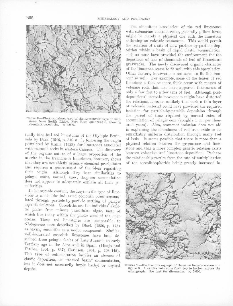
B98 MLNERALOGY AND PETROLOGY

FIGURE 6.-Eleetron micrograph of the Laytonville type of lime­stone from Smith Ridge, Fort Ross qundrangle, showing abundant cocco-liths. X 5,000.

tually identical red limestones of the Olympic Penin­sula by P.ark (1946, p. 310-311), following the origin postulated by Kania ( 1929) for limestones associated with volcanic rocks in western Canada. The discovery of the organic nature of a large proportion of the micrite in the Franciscan limestones, however, shows that they are not chiefly primary chemical precipitates and requires a reassessment of the ideas regarding their origin. Although they bear similarities to pelagic oozes, normal, slow, deep-sea accumulation does not appear to adequately explain all their pe­culiarities.

In its organic content, the Laytonville type of lime­stone is much like indurated coccolith oozes aceumu­lated _through particle-by-particle settling of pelagic orgamc skeletons. Coccoliths are the individual skele­tal plates from minute unicellular algae, most of which live today within the .photic zone of the open oceans. These red limestones are comparable to Olobigerina ooze <described by Black ( 1956, p. 173) as h~ving coccoliths as a major component. Similar, well-mdurated coccolith limestones have been de­scribed from pelagic facies of Late Jurassic to early T~rtiary age in the Alps and in Spain (Honjo and Fis_cher, 1964, p. 837; Garrison, 1964, p. 103-145). This type of sedimentation implies an absence of clastic deposition, or "starved basin" sedimentation but it does not necessarily imply bathyl or abyssai depths.

The ubiquitous association of the red limestones with submarine volcanic rocks, generally pillow lavas, might be merely a physical one with the limestone collecting on volcanic seamounts. This would permit the isolation of a site of slow particle-by-particle dep­osition within a basin of rapid clastic accumulation, such as must have provided the environment for the deposition of tens of thousands of feet of Franciscan graywa:cke. The newly discovered organic character of the limestone seems to fit well with this speculation. Other factors, however, do not seem to fit this con­cept so well. For example, some of the lenses of red limestone ;a foot or more thick occur with masses of volcanic rock that also have apparent thicknesses of only a few feet to a few tens of feet. Although post­depositional tectonic movements might have distorted the relations, it seems unlikely that such a thin layer of volcanic material could have provided the required isolation for particle-by-particle deposition through the period of time required by normal rates of accumulation of pelagic ooze (roughly 1 em per thou­sand years) . Also, seamount isolation does not aid in explaining the abundance of red iro.n oxide or its remarkably uniform distribution through many feet of beds. It seems possible that there is more than a physical relation between the gre~nstone and lime­stone and that a more complex genetic relation exists between volcanism and limestone deposition. Perhaps the relationship results from the rate of multiplication of the coocolithophorids being greatly increased lo-

FIGURE 7.-Electron micrograph of the same limestone shown in figure 6. A calcite vein runs from top to bottom across the micrograph. See text for discussio.n. X 5,000.

GARRISON AND BAILEY B99

~ cally by the action of lava extrusion through either ( 1) warming of the water and increasing the nutrient supply, or (2) the addition of calcium from the lava. As indiowted by Bailey and others (1964, p. 77), chemical analyses of pillow lavas and aquagene tuffs in the Franciscan strongly suggest that large amounts of calciuni were extracted from the volcanic material rrnd added to the sea water.

The origin of the iron-free Calera type of limestone remains even more obscure. The preliminary electron­microscope studies sho,Yecl only scattered nannoplank­ton and suggested greater recrystallization than in the Laytonville type. ""\Ve cannot yet be sure if many more nannoplankton "·ere present and have been de­stroyed, or if a larger proportion of the micrite may have been inorganic. Strictly diagenetic processes seem inadequate to explain the poor preservation of coccoliths in the Calera limestones we studied, inas­much as calcite coccoliths have been shown to be very resistant to alteration (Robertson, 1964, p. 544). Thus, although the electron-microscope studies of the Calera type of limestone tend to justify considering it as different from the Laytonville type, more samples must be studied before conclusions regarding the con­tent or origin of its micrite are warranted.

POSSIBILITIES FOR BIOSTRATIGRAPHIC DATIN·G

Study of the nannoplankton offers a possibility for finer ·and more widespread biostratigraphic elating within the Franciscan. No attempt has been made to compare the forms observed in this study with known and described species, although the degree of coccolith preservation (figs. 8 and 9) indicates that for the Laytonville limestones this could be done. One might expect some difficulties because of the general lack of knowledge of these nannoplankton, their taxonomy, and their stratigraphic ranges, and because of the problems introduced by comparing electron micro­graphs of replicas with free specimens observed with the optical microscope (Honjo and Fischer, 1964, p. 839; Bramlette and Martini, 1964, p. 293-294). The nannoplankton, however, can be expected to oc.cur also throughout the Franciscan in shales from which free specimens might be extracted and concentrated for study. In the latter case, an electron microscope, al­though helpful, is not a necessity as most biostrati­graphic studies of the nannoplankton till now have been made with the optical microscope. If the nanno­plankton can be recovered from these genera,Hy un­fossiliferous rocks, they should provide a much-needed means of correlating or differentia,ting sequences within the Franciscan Formation.

~ ~""').,

' \ . ''l

'.~~

FIGURE 8.-Electron micrograph of the Laytonville type of lime­stone from Smith Ridge, Fort Ross quadrangle, showing a large coccolith surrounded by smaller coccoliths and corutain­ing fragments of coccoliths within a central cavity. X 5,000.

ACKNOWLEDGMENTS

The support of the Petroleum Research Fund of tlH' American Chemical Society (contract PRF 1114-81-A2) made possible the laboratory investigation of the first author and is most gratefully acknowledged. Use of an electron microscope was kindly made avail­able by Dr. L . I. Rebhun, Department of Biology, Princeton University. Dr. A. G. Fischer, of Princeton University, gave helpful advice during aJll stages of the investigation. The laboratory work was conducted while the first author was a postdoctoral fellow at Princeton University.

FIGURE 9.-Electron micrograph of same limestone as in figure 7, showing a very well preserved coccolith . X 10,000.

BlOO Mr.NERALOGY AND PETROLOGY

REFERENCES

Bailey, E. H., Irwin, W. P., and Jones, D. L., 1964, Franciscan and related rocks and their significance in the geology of western California: California DiY. Mines and Geology Bull. 183, 177 p.

Bathurst, R. G. C., 1958, Diagenetic fabrics in some British Dinantian limestones : Liverpool and Manchester Geol. Jour., v. 2, p. 11-36.

Black, Maurice, 1956, The finer constituents of Globigcrina ooze [abs.] : Internat. Geol. Gong. 20th, Mexico City 1956, Re­sumeres de los Trabajos Presentados, p. 173.

Bramlette, l\f. N., and Martini, E., 1964, The great change in calcareous nannoplankton fossils between the Maestrichtian and Danian: Micropaleontology, v. 10, p. 291-322.

Bronnimann, Paul, 1955, Microfossils incertae seclis from the Upper Jurassic ancl Lower Cretaceous of Cuba : Micro­paleontology, Y. 1, p. 28-51.

Garrison, R. E., 1004, Jurassic and early Cretaceous sedimenta· tion in the Unken Valley area, Austria: Princeton Univ., Ph.D. thesis, 188 p.

Honjo, Susumu, and Fischer, A. G., 1964, Fossil coccoliths in limestone examined b:r electron microscopy: Science, v. 144, p. 837-839.

--- 1965a, Thin sections and peels for high magnification study and phase-contrast microscopy, in Kummel, Bernhard, and Raup, D. 1\I., eds., Handbook of paleontological tech­niques: San Francisco, ,V. H. Freeman and Co., p. 241-247.

--- 1965b, Paleontological investigation of limestones by electron microscope, in K.ummel, Bernhard, and Raup, D. l\1.

eds., Handbook of paleontological techniques: San Fran­cisco, W. H. Freeman and Co., p. 326-334.

Kania, .J. E. A., 1929, Precipitation of limestone by submarine vents, fwnaroles, and lava flows: Am. Jour. Sci., 5th ser., v. 18, p. 347-359.

KUpper, Klaus, 1955, Upper Cretaceous Foraminifera from the "Franciscan Series," New Almaden district, California: Cushman Found. Foram. Research Contr., v. 6, p. 112-118.

Leighton, M. ,V., and Pendexter, Charles, 1962, Carbonate rock types, in Ham, ,V, E., and Pray, L. C., eds., Classification of carbonate rocl\:s : Am. Assoc. Petroleum Geologists Mem. 1, p. 33-61.

Loeblich, A. R., Jr., and Tappan, H. R., 1961, Cretaceous plank­tonic Foraminifera, pt. 1, Cenomanian: Micropaleontology, v. 7, no. 3, p. 257-304.

Park, C. F., .Jr., 1946, The spilite and manganese problems of the Olympic Peninsula, Washington: Am .. Jour. Sci., new ser., Y. 244, p. 305-323.

ProYasoli, Luigi, 1963, Organic regulation of phytoplankton fer­tility, in Hill, M. N., The sea, v. 2: New York, Interscieuce Publishers, v. 165-219.

Reinhard, Max, and 'Venk, Eduard, 1961, Geology of the Colony of North Borneo: Borneo (British Terr.) Geol. SurYey Dept. Bull. 1, 160 p.

Robertson, E. C., 196-l, Experimental consolidation of carbonate mud [abs.] : Am. Assoc. Petroleum Geologists Bull., v. 48, p. 544.

Thalmann, H. E., 19-!2, Globotruncana in the l!'ranciscan lime­stone, Santa Clara County, California [abs.] : Geol. Soc. America Bull., v. 3, no. 12, pt. 2, p. 1838.

GEOLOGICAL SURVEY RESEARCH 1967

X-RAY DETERMINATIVE CURVE FOR SOME ORTHOPYROXENES

OF COMPOSITION Mg 48•85 FROM THE STILLWATER COMPLEX, MONTANA

By GLEN R. HIMMELBERG and EVERETT D. JACKSON, Menlo Park, Calif.

Abstract.-An X-ray determinative curve for 12 chemically analyzed orthopyroxenes based on ~2e (131) orthopyroxene- (111) lithium fluoride gives the regression equation ~2e (CuKa 1)

=4.112-0.009132Mg. Two sigma for the regression equation is ± 0.012°20, which corresponds to about ± 1.3 percent l\1g.

An X-ray determinative method similar to that developed by Jackson (1960) for natural olivines was applied to 12 orthopyroxenes from the Precambrian Stillwater complex, l\1ontana. These orthopyroxenes were separated by the method described by Schoen and Lee (1964). Purity of the separates was estimated fron1 grain counts, and ranged between 98.9 and 99.7 percent. Two of the samples were split to make hidden duplicates which were then treated as separate samples. The 14 samples were chemically analyzed, and the l\1g content of each sample was calculated as the ionic ratio of l\1g to total octahedral cations. Splits of each of the 14 analyzed samples were divided into 3 separate parts for X-ray examination. These 42 separate parts were assigned random numbers to determine run order, mixed with about 10 percent lithium fluoride (reagent), and prepared us slurries on cover glasses % inch in diameter. 'rhe cover glasses containing the slurries were placed in a rotating sample holder, and sample heights were adjusted by placing prepared disks of the proper thickness under the samples. Each of the 42 subsamples was allowed to oscillate up and down twice between 34.5° u.nd 40°28 on a diffractometer using copper radiation and a focusing monochrometer. A 1° divergent slit, a 4° preslit, and a 1° receiving slit were used. The scan speed was }~ 0 per minute, and the chart scale was 2 inches per degree 28. The dis­tances between the orthopyroxene (131) peak and the lithium fluoride (111) peak were measured directly in degrees from the charts and were compiled; means and standard deviations of d28 were calculated from them. Mg content, calculated fi·on1 the analyses, and X-ray data are summarized in table 1.

The information in table 1 forms the basis for the determinative curve in figure 1. The X-ray data are plotted directly as degrees d28 (Cul(a1) on the ordinate, the l\1g value on the nbscissa. A regression analysis was made considering the 14 measurement sets to represent individual samples, using the average X-ray parameter d28 as the dependent variable, and taking the chemically derived value of l\1g as the independent variable. The linear equation is:

d28 (CuKa1) (131) orthopyroxene- (111) fluoride=4.112-0.009132l\1g.

lithium

Two sigma for the regression equation is ± 0.012° 28, which corresponds to about ± 1.3 percent l\1g.

The determinative curve shown is based on ortho­pyroxenes from n. single petrographic province and with similar Ininor-element contents. The aluminum con­tent ranges from 0.038 to 0.119 ion per formula of 6

TABLE 1.-Mg content and X-ray measurements of orthopyroxene samples

Field No.

55 BE-L ____________ _ 531~-2 _____________ _ 53~B-11 ____________ _ 55~B-1 3 ____________ _

.55BE-2 _____________ _ 55BE-4 _____________ _ 55BE-7 --------------52BE-35 ____________ _ 52BE-29 ____________ _ 55MV-32 ____________ _ 55MB-2 4 ____________ _ 55MV-29 ____________ _ 55MV-26 ____________ _ 61SC-B _____________ _

Mgt

48.69 52.47 54.27 54.23 72.08 72.25 79 .. 04 82.49 83.51 82.98 83.02 82.91 84.08 83.93

Mean of 12 readings of 29u1 (ortho­

pyroxene) -29111 (LiF) (degrees) 2

3.665 3.635 :3.621 :3.612 3.461 3.449 3.400 3.365 3.358 3.348 3.352 :~.349 3.343 3.339

Standard deviation of 12 readings (degrees)

0.0139 .0156 .0108 .0086 .0089 .0067 .0106 .0120 .0097 .0064 .0072 .0073 .0108 .0130

t Ionic ratio or Mg to the sum of Mg, Fe+2, Mn, Ni, Co, Cu, A! VI, Fe+3, Cr, V, Sc, Ti, Zr, Mo, and Sn X 100.

2 CuKa 1 radiation. 3 Hidden duplicate of 53NB-ll. 4 Hidden duplicate of 55MV -32.

U.S. GEOL. SURVEY PROF. PAPER 575-B, PAGES Bl01-Bl02

B101

B102 MINERALOGY AND PETROLOGY

oxygens (0.86 to 2.87 weight percent Al 20 3); the calcium content ranges from 0.045 to 0.112 ion per formula of 6 oxygens (1.10 to 2.98 weight percent-CaO). Some of this calcium however, is present in clinopyr.oxene exsolution lamellae. Hess (1952), l{uno (1954), and Zwaan (1954) have sliown that orthopyroxene X-ray parameters are affected by aluminum and calcium contents. 'fhe determinative curve should therefore be used with caution in estimating or comparing orthopyroxenes from different chemical, thermal, or barometric environments.

REFERENCES

Hess, H. H., 1952, Orthopyroxenes of the Bushveld type, ion substitutions and changes in unit cell dimensions: Am . . Jour. Sci., Bowen volume, p. 173-187.

.Jacl(son, E. D., 1960, X-ray determinative cun-e for natural olivine of composition Foso-oo: Art. 197 -in U.S. Geol. Suney Prof. Paper 400-B, p. B432-B434.

Kuno, Hisashi, 1954, Study of orthopyroxenes from volcanic rocks: Am. l\lineralogist, v. 39, p. 30-46.

Schoen, Robert, and Lee, D. E., 1964, Successful separation of silt-size minerals in heavy liquids, t'n Geological Surwy Research 1964: U.S. Geol. Surwy Prof. Paper 501-B, p. B154-BHi7.

Zwaan, P. C., 19i34, On the determination of l)~Toxenes by X-l·ay powder diagrams: Leidse Geol. Mededeel, v. 19, p. 167-276.

~ . 3. 7 3 r-r-r-r--r-r--r-r--r-r-r-r-,-,.--.-.--r-r-r-r-,rT""'1r--r-r-r..--r-TT'".--r--r-T".,-,-.,-,--,-,-,..,---rn LLJ c::: (!) LLJ 0

~

T LLJ z LLJ X 0 c::: >­c.. 0 J: 1-c::: 0

<t:> N

<I

85 80 75 70 65 60 55 50 45

Mg (IONIC RATIO MgXlOO/TOTAL OCTAHEDRAL CATIONS), IN PERCENT

~"'IGURE 1.-X-ray determination curve for orthopyroxenes of composition Mg4s-s!;.

GEOLOGICAL SURVEY RESEARCH 1967

SERPENTINE-MINERAL ANALYSES AND PHYSICAL PROPERTIES

By NORMAN j. PAGE and ROBERT G. COLEMAN, Menlo Park, Calif.

A.bstract.-Purified separates of serpentine minerals were prepared from seven serpentinite samples from California and New Zealand. Chemical and spectrographic analyses for the separates are presented, together with their optical, physical, and X-ray properties. A new serpentinite mineral assemblage consisting of clinochrysotile and corundum with or without magnetite was found in a vein cutting massive serpentinite at New Idria, Calif.

Chemical analyses of purified serpentine 1ninerals, accompanied by X-ray identification and physical de­scriptions, are sparse in modern literature. The pur­pose of this paper is to present new data on analysed serpentine minerals that have been ·used as standards in n. more comprehensive long-term study of the ser­pentines (Page, 1966; Hostetler and . others, 1966) by .the U.S. Geol10gical Survey. Each sample was carefully purified before analysis to insure that the analyzed material consisted of a single phase. Stand­ard heavy-liquid techniques were used to separate the serpentine minerals from the ·parent serpentinites, ex­cept for fibrous clinochrysotile. This mineral was disaggregated and heavy 1ninerals intergrown with it were removed by repeated elutriation. The ter­minology and classification of the serpentine minerals used in .this report are those o~ Faust and Fahey ( 1962) and 'Vhittaker and Zussman ( 1956).

Acknowledgments.-The chrysotile sample frmn the Union Carbide Corp. plant was supplied by Dr. Fred Mumpton. ~1iss Terry Clark, U.S. Geological Sur­vey, provided some of the mineralogical support on this study.

NEW CH'EMICAL AND MINERALOGICAL DATA ON SERPENTINE MINERALS

Complete chemical analyses of-the serpentine minerals studied are given in table 1 and are comparn,ble with analyses by Ftiust and Fahey (1962). Spectrographic analyses and descriptions of the samples are also given in table 1.

Table 2 presents indexed d-spacings and intensities for six of the specimens. In sample 3, traces of clino­chrysotile are present; in sample 5, traces of lizardite are present and in sample 6, peaks of corunduri1 are present. The d-spacings are similar to those given by vVhittaker and Zussmnn ( 1965) and completely charac­tet:ize the serpentine species for each sample.

Optical measurements of the different serpentine minerals (table 3) were made in sodium light. Fibers of sample 4 were impossible to mount on a spindle stage, so only an index parallel to the fiber axis (a) could be 'measured, whereas in samples 5 and 6 of clinochrysotile, a and (3 appeared to be equal. Refined unit-cell parmn­eters and observed and calculated specific gravities are also given in table 3.

The distribution of cations between octahedral and tetrahedral positions, on the basis of 18 anions per Inin­e.ral for 6 samples, is showi1 in table 4. No calculations were made for sample 6 because of the abundance of Al20a that is present as corundum.

The chemical singularity of antigorite is clearly dem­onstrat·ed both in tables 1 and 4. The antigorites have a ratio of FeO to Fe2 0 3 greater than one, and appar­ently all the alumina is present in octahedral coordina­tion and none in tetrahedral coordination; in lizardite and clinochrysotile the reverse is true. · The data also suggest that lizardites differ chemically frmn clinochry­sotiles by having a large amount of total iron (Page, 1966).

ASSEMB-LAGE CLINOCHRYSOTILE AND CORUNDUM

In sample 6, the assemblage clinochrysotile + corun­dum with or without magnetite is present. The corun­dum is irregularly distributed and occurs as colorless to pale-yellow euhedral and subhedral grains varyiilg in size from submicroscopic to 0.1 mm in diameter. Some sections subparallel with (0001) exhibit a small 2 V that is anomalous ·for an uniaxial mineral but that is common in oorundum (De:er and others, 1962). The corundum was concentrated by dissolution of the clino­chrysotile in a mixture of HCl, H 2S04, HN03 , and HF.

U.S. GEOL. SURVEY PROF. PAPER 575-B, PAGES B103-Bl07

B103

B104 MUNERALOGY AND PETROLOGY

TABLE 1.-Chemical and spectrographic analyses of serpentine minerals from New ldria, Calif., and New Zealand

[Gravimetric chemical analyses by L. B. Beatty, U.S. Geol. Survey; spectrographic analyses by R. E. Mays, U.S. Geol. Survey]

Antigorite Lizardite Clinochrysotile --------,-------------,---------------------1-----------·.-----------~-----------~----------

la 3

CHEMICAL ANALYSES (WEIGHT PERCENT)

Si02---------------------------- 4~ 2 AJ203--------------------------- . 90 Fe20a- _ _ _ _ _ _ _ _ _ _ _ _ _ _ _ _ _ _ _ _ _ _ _ _ _ _ . 27

FeO------------------------~--- 2 1 MgO _ _ _ _ _ _ _ _ _ _ _ _ _ _ _ _ _ _ _ _ _ _ _ _ _ _ _ 40. 1 CaO____________________________ . 02

N a20 __ ------------------------- ----------K 20 _______ --------------------- ----------TiO~--------------------------- . 01 Cr20a- _ _ _ _ _ _ _ _ _ _ _ _ _ _ _ _ _ _ _ _ _ _ _ _ _ _ . 22 NiO____________________________ . 13 MnO _ _ _ _ _ _ _ _ _ _ _ _ _ _ _ _ _ _ _ _ _ _ _ _ _ _ _ · . 02 H20+- _______ -_ -_______ -_ -_ _ _ _ _ _ 11. 9 H2o-___________________________ . 15

TotaL ___________________ _ 100. 02

44. 8 .5 .2

2. 2 39. 9

. 02 0 00 . 00 .0 . 15 .5 . 02

11. 8 . 13

99. 9

43. 1 1. 3 . 80

2. 6 39. 8

. 02 --------------------

. 002

. 06

.11

. 03 11. 9

. 07

99. 79

41. 1 42. 2 0 78 . 66

2. 4 1. 2 0 21 . 09

41. 5 41. 7 . 02 0 01

---------- -------------------- ----------

0 003 0 002 . 20 . 02 .11 . 04 . 05 . 06

13. 3 13. 3 . 63 . 95

100. 30 100. 23

SPECTROGRAPHIC ANALYSES (PARTS PER MILLION)

I 6

41. 4 32. 1 . 70 34.6

1.4 . 82 1. 3 1.3

41. 4 20.9 . 04 '84

---------- -------------------- ----------

. 002 . 18

. 01 '009 '02 0 002 . 04 '04

13. 0 7. 6 . 63 1.4

----------99. 94 99. 78

Cu_____________________________ 7 13 5 8 2 18. 70 Sn_ _ _ _ _ _ _ _ _ _ _ _ _ _ _ _ _ _ _ _ _ _ _ _ _ _ _ _ _ _ _ _ _ _ _ _ _ _ _ _ _ _ _ _ _ _ _ _ _ _ _ _ _ _ _ _ _ _ _ _ _ _ _ _ _ _ _ _ _ _ 20 < 10 < 10 Mn_____________________________ 110 100 220 360 420 320 280 Co_____________________________ 30 14 26 40 40 46 26 Ni______________________________ 1, 000 1, 200 900 900 300 160 17 v______________________________ 14 8 16 <1o <1o <10 30

41. 0 .7

1.3 . 95

40.7 0 13 . 04 . 00

<. 01 . 23 . 22 0 07

12. 8 1.5

-----99. 6

460 70

1, 700 <20 Zr _ _ _ _ _ _ _ _ _ _ _ _ _ _ _ _ _ _ _ _ _ _ _ _ _ _ _ _ _ _ _ _ _ _ _ _ _ _ _ _ _ _ _ _ _ _ _ _ _ _ _ _ _ _ _ _ _ _ _ _ < 10 < 10 < 10 440 _________ _

Sc_ _ _ _ _ _ _ _ _ _ _ _ _ _ _ _ _ _ _ _ _ _ _ _ _ _ _ _ _ _ < 4 _ _ _ _ _ _ _ _ _ _ 12 _ _ _ _ _ _ _ _ _ _ _ _ _ _ _ _ _ _ _ _ _ _ _ _ _ _ _ _ _ _ _ ________ _ 4 Sr _ _ _ _ _ _ _ _ _ _ _ _ _ _ _ _ _ _ _ _ _ _ _ _ _ _ _ _ _ _ _ _ _ _ _ _ _ _ _ _ _ _ _ _ _ _ _ _ _ _ _ _ _ _ _ _ _ _ _ _ < 4 < 4 < 4 60 Ba _ _ _ _ _ _ _ _ _ _ _ _ _ _ _ _ _ _ _ _ _ _ _ _ _ _ _ _ _ _ _ _ _ _ _ _ _ _ _ _ _ _ _ _ _ _ _ _ _ _ _ _ _ _ _ _ _ _ _ 8 < 4 < 4 65 9

30 1, 000

B _ _ _ _ _ _ _ _ _ _ _ _ _ _ _ _ _ _ _ _ _ _ _ _ _ _ _ _ _ _ 20 _ _ _ _ _ _ _ _ _ _ _ _ _ _ _ _ _ _ _ _ 60 60 < 20 100 Cr______________________________ 1, 500 1, 200 400 1, 400 1, 400 420 650

1 Analysis of a mixture of corundum and clinochrysotile.

1. Field No. 38-NZ-62-5; lab. No. 63M-409. Massive greenish-black antigorite from a rock with the assemblage antigorite, talc, and magnetite. This same material produces a clear translucent gem-quality material referred to as bowenite (Reed, 1957). Veins in dunite mylonite, Milford Sound, South Island, New Zealand (Coleman, 1966).

la. Lab. No. 65M-643. Same as sample 1, but a different separate. 2. Field No. 94-NZ-62; lab. No. 63M-410. Antigorite from a rock with an interlock­

ing matte of antigorite laths (0.5-0.1 mm length) perpendicular to each other with the assemblage antigorite and magnesite with or without talc, magnetite, or olivine. This sample is from the same area as the antigorite discussed by Zuss­man (1954); geology and petrology described by Coleman (1966). Lens in biotite-garnet schists, Griffin Range, Westland, New Zealand.

3. Field No. 19-NI-63A; lab. No. 63M-826. Light-green lizardite from a vein with mesh structure cut by cross-fiber chrysotile veins with the assemblage lizardite and magnetite with or without heazlewoodite and clinochrysotile. Vein in serpentinite, Joe No. 5 Pit, Union Carbide Corp., New Idria, San Benito County, Calif. Tak('n from sa.me outcrop as sample 4.

4. Field No. 19-NI-63B; lab. No. 63M-S27. White to pale-green clinochrysotilo slip fiber matte composed of fine "thread-like" material, consisting of serpentine encrusting massive serpentinite. Joe No. 5 Pit, Union Carbide Corp., New Idria, San Benito County, Calif. Taken from same outcrop as sample 3.

5. Field No. 14-NI-63A; lab. No. 63M-828. Green to black massive bladed clino· chrysotile vein with traces of lizardite; in thin section, perpendicular to blades; pseudoisotropic. Vein in serpentinite, Butler Estate chrome mine, New Idria, San Benito County, Calif. Taken from same outcrop as sall),ple 6.

6. Field No. 14-NI-63C; lab. No. 63M-829. A mixture of clinochrysotile and corun­dum from a ~-to 1~-inch vein of clinochrysotile and magnetite with or without corundum. Cross-fiber vein in serpentinite, Butler Estate chrome mine, New Idria, San Benito County, Calif. Taken from same outcrop as sample 5.

.. Union Carbide mill product; lab. No. 65M-1119. Clinochrysotile, representative mill product from Union Carbide Corp., King City, Calif., plant. From Joe No.5 Pit, Union Carbide Corp., New Idria, San Benito County, ColiC.

TABLE 2.-lndexed d-spacing and intensity for serpentine minerals 1 2

(Symbols: vs, very strong; s, strong; m, moderate; mw, moderately weak; w, weak; vw, ,·cry weak)

Antigorite Lizardite Clinochrysotile

1 2

-------- -----

(hi.Z) d(A) I d(A) I (hkl)

----

001 7. 30 vs 7. 29 VS 001 6. 43 '" 020

401 6. 23 w 610 5. 82 '" 022, 111 311 5. 15 \Y 002 5'11 4. 93 lllW 020 4. 64 mw 420 4. 26 "' 200 711 4. 20 w 130, 210 021 4. 01 vw 901 3. 99 vw 131 12. 0. 0, 002 3. 62 s 3. 61 s 003 IT. 4. o 3.44 w IT. 2. 1, 331 2. 794 \Y

730,422 2. 790 w 15. 0. 1, 622 2. 667 vw 12. 0. 2, 731, } 2. 596 w 5 204 I. 4. 20 16. 0. 1 2. 530 VS 2. 525 VS 93I 2.458 m 004 17. 0. 1, 203 2.423 w 2. 429 '" 14. 0. 2 2. 386 w 203 141,141,640 2. 210 w 5 206 832,901 2. 172 m 024, 114, 311 21. 1. 1 1.940 '" 18. 2. 2, 842 1. 833 '" 060 15. 1. 3, 151, } 1. 814 w 1. 812 '" 20. 1. 2, 240 061 650 1. 795 w 005 314 1. 780 w 751,20. 2. 2 1. 741 w 1. 742 w 062 23. 2. 1 1. 709 vw 261 951 1. 702 m 22. 1. 2 1. 694 m 170 452 1. 627 w 402, 262 22. 4. 0 1. 508 '" 26. 4. 2 1. 278 vw 006 36. 0. 0, 13. 6. 3 1. 209 vw 26. 5. 2 1. 181 vw

-

• See table 1 for sample descriptions. z Indexing by computer program 9214, U.S. Geol. Survey, Menlo Park, Calif. 1 Corundum d-spacing.

---

3 4

------- ---------------

d(A) I (hkl) d(A) I d(A) -------- ---- --------

7. 37 vs 002 7. 15 -------- 7. 31 4. 61 m 020 4. 53 -------- 4. 57

I12 4. 06 -------- 4. 05 3.88 w 3. 66 vs 004 3. 66 -------- 3. 65

023 3. 36 --------2. 669 w 2. 603 vw

201 2. 588 --------2. 504 s 2. 455 vs 4 003 2. 45

~02,006 2.435 --------203 203 2. 270 204, I16 2. 205

2.095 w 204,007,043 2.083 -------- 2. 092 ~24, 205 1. 991 --------240

1. 825 V"' 008,205 } 1. 823 -------- 1. 827 I35

1. 797 vw 1. 745 vw 206,240 1. 744 -------- 1. 744 1. 700 vw

153 1. 635 --------1. 539 s 060 1. 535

I38 1. 524 --------1. 505 w 4 061 1. 506 1. 459 m 0. 0. 10, 063 1. 466 -------- 1. 463

1. 417 '" 4 062

1.311 \Y 2. 1. 10, } 1. 310 -------- 1. 313 262, 401

1. 279 m 1. 252 vw 405

424,265 1. 222 1. 215 vw 3 006 1. 219

~54, 265,355 } 355 ---

4 Lizardite d-spacing. 5 Clinochrysotile d-spacing.

5

I ---

VS m

V"'

s

vw

'" w w

"' w

m

w

"' \Y

----------------

6

d(A) ----

7.34 4. 55

3. 66 3 3. 48

3. 34

3 2. 55

2.453 3 2. 382

2. 207 2. 084 2. 010 1. 913

3 1. 601 1.534

1. 489

3 1. 405 l. 311

1. 238

1. 189

I

-----

------------

------------------

------

------------

------------------------

------------

------

------------

------

------

"'d > 0 tr.l

~ t::::l

(') 0 t'4 tr.l ~

~

tJ:1 ....... ~

TABLE 3.-0ptical and physical properties of serpentine minerals 1

Antigorite Lizardite Clinochrysotile

1a 3 5 6

OPTICAL PROPERTIES

1. 569 ± 0. 002 1. 545 ± 0. 002 aNa---------------------­~Na----------------------­~Na-----------------------

2Va----------------------Birefrigence ______________ _

1. 563 ± 0. 001 1. 565± . 002 1. 570± . 002

73±5° . 007

1. 562 ± 0. 002 1. 565± . 002 1. 567± . 002

78° . 005

1. 556-1. 558 1. 565-1. 567 1. 572-1. 569

61±3° . 016- . 011

1. 561 ± 0. 002 1. 565± . 002 1. 567 ± .. 002

Small . 006

---- -~-- ~~~~~:-~~~-I-----~--~·~~~-:-~~~ -I----------~--~~~

a _____________________ A __ 43. 445 ± 0. 007 --------------b~ ____________________ A __ 9. 374± . 002 ----------- .... --c _____________________ A __ 7. 294± . 002 --------------~----------------degrees __ 90°47. 9' ± 0. 7' --------------Cell volume (obs) ______ Aa __ 2, 907. 2± . 8 --------------·Cell volume (calc) ______ A a __ ------------------ 2,925. 4

0 bserved ________________ -1- ________________ -1 2. 605-2. 610 Calculated 2________________ 2. 56 _____________ _

1 See table 1 for sample descriptions.

PHYSICAL PROPERTIES Unit-eell data 2

43. 53± 0. 01 9. 259± . 003 7. 263± . 007

91°8. 4' ± 1. 6' 2, 927. 2± 2. 3 2,886. 0

Speeifie gravity

2. 65 2. 61

5. 339 ± 0. 003 9. 226± . 002 7. 315± . 006

goo 360. 3± . 3 363. 5

2. 55±0. 03 2. 57

5. 3143 ± 0. 0002 9. 2533 ± . 0004

14. 6307 ± . 0003 92° 52. 4' ± 0. 2'

718. 56± . 02 ------------------

2. 56

2 Computer program 9214, least-squares unit-cell refinement translated into Algol from original Fortran 4,U.S. Geol. Survey, Menlo Park, Calif.

5. 3129 ± 0. 0009 9. 120 ± . 003

14. 637 ± . 002 93°9. 8' ± 0. 6'

708. 2± . 3 731. 2

2. 53±0. 01 2. 61

5. 325±0. 00 9. 173± . 00

14. 669± . 00 93°20. 6' ± 1. 6'·

715. 3± . 3 ---------------

3 8

to ~

0 O"l

~

~ ~ 0 0 1-<l

> z t:!

'"d t'j t-3 !:tl 0 t"4 0

~

PAGE AND COLEMAN B107

TABLE 4.-Structural formulas of the serpentine minerals, calculated by the hydrogen equivalent method based on 18 anions per formula 1 2

Antigorite Lizardite Clinochrysotile

Ia 3

------------------------------------1- -------l-------------------1------------------l~ --------1-------

Tetrahedral {~1::-_-~ = = = = = = = = = = = = = = = = = = = = = = = = = ____ ~·- ~~~ _____ ~·- ~~~ _____ ~·- ~~~ _ 3

: ~~~ 3: ~~~ 3: ~i~ 3: ~~~ TotaL_______________________ 4. 146 4. 201 4. 067 3. 918 3. 996 3. 910 3. 975 AI+S____________________________ 4. 100 . 055 0. 145 ---------- ---------- ---------- ----------Cr+s____________________________ . 016 . 011 . 005 . 015 . 002 . 001 . 017 Fe+s____________________________ • 019 . 014 . 057 . 168 . 084 . 098 . 093

Octahedral TiH____________________________ · 001 ---------- ---------- ---------- ---------- ---------- · 001

Ni~;:=========================== ··5: 8~8

5: g~~

5: gg~

5: b8~

5: bbg

5: b5~ 5

: b~~ Fe+2____________________________ . 165 . 173 ·. 205 . 016 . 007 . 101 . 076 Mn+2 _ _ _ _ _ _ _ _ _ _ _ _ _ _ _ _ _ _ _ _ _ _ _ _ _ _ _ . 002 . 002 . 002 . 004 . 005 . 003 . 006

TotaL________________________ 5. 919 5. 869 6. 019 5. 979 5. 879 5. 932 5. 976 OH-1___________________________ 7. 445 7. 380 7. 489 8. 272 8. 248 8. 438 8. 115 o-2_____________________________ 10. 555 10. 620 10. 511 9. 728 9. 752 9. 562 9. 885

• Soc table 1 for sample descriptions. 2 Computer program Mineral No11ns 9377, U.S. Geol. Survey, Menlo Park, Calif.

REFERENCES

Coleman, R. G., 1966, New Zealand serpentinites and asso­ciated metasomatic rocks: New Zealand Geol. Survey Bull. 76, 102 p.

Deer, ,V. A., Howie, R. A., and Zussman, J., 1962, Non-silicates, v. 5 of Rock-forming minerals: London, Longmans, Green, nnd Co., Ltd., 371 p. ·

]j"'nust, G. T., and ]j"'ahey, J .. J .. 1962, The serpentine-group min­erals: U.S. Geol. Survey Prof. Paper 384-A, p. Al-A92.

Hostetler, P. B., Coleman, R. G., Mumpton, F. A., and Evans. B. W., 1966, Brucite in Alpine serpentinites: Am. Mineralo­gist, v. 51, nos. 1-2, p. 75-98.

241-334 0----:67---8

Page, N. J., 1966, Mineralogy and chemistry of the serpentine­group minerals and the serpentinization process : California Unh·., Berl\:eley, Ph. D. thesis.

Reed, J. J., 1957, Use of the terms greenstone, nephrite, bowenite, and jade: Polynesian Soc. Jour., v. 66, no. 2, 2 p.

'Vhittaker, E. J. ,V., and Zussman, J., 1956, The characteriza­tion of serpentine minerals by X-ray diffraction: Mineralog. Mag. [London], v. 31, no. 233, p. 107-126.

Zussman, J., 1954, Investigation of the crystal structure of antigorite: Mineralog. Mag. [I..~ondon], v. 30, no. 227, p. 498-512.

GEOLOGICAL SURVEY RESEARCH 1967

A NEW(?) YTTRIUM RARE-EARTH IRON ARSENATE MINERAL

FROM HAMIL TON, NEVADA

By ARTHUR S. RADTKE and CHARLES M. TAYLOR/ Menlo Park, Calif., Palo Alto, Calif.

Abstract.-~iagnetite grains in manganoan calcite or "black calcite" associated with silver ores at Treasure Hill, Hamilton, Nev., contain significant amounts of a new ( ?) Y·ttrium rare-earth iron ar1senate mineral. Chemical analyses made with the elec­tron microprobe analyzer shows the approximate formula to be

3 ( Y,Ce,Nd,Dy,Gd,Er) 20a · Fe20a · 2A~O" ± 14H20.

Small particle size and distribution of the rare-earth-ricll mineral precluded obtaining X-ray powder data. Certain physi­cal and optical data are given.

A sample of manganoan calcite, "black calcite," from Treasur~ Hill, Hamilton, Nev. (an abandoned mining town about 40 miles west of Ely, in east-central Ne­vada), collected by D. F. Hewett, of the U.S. Geological Survey, contains a rare-earth-rich mineral disseminated through grains of magnetite. The formula of the mineral is approximately

3(Y,Ce,Nd,Dy,Gd,Er)203 • Fe203 ·2As205 ± 14H20.

The composition, as determined with the Materials Analysis Co. model-400 electron microprobe analyzer and calculated as oxides, is shown in table 1. Iron, vanadium, and manganese have been calculated arbi­trarily as the highest valence oxides. Elemental weight percentages of arsenic and iron were determined to be 17.3 and 5.9, respectively. The molecular ratio of As205 to Fe203 is then approximately 2 to 1.

The only known yttrium arsenate mineral is retzian, which is distinctly different in composition. Palache and others (1951, p. 795) reported that retzian contains 19.2 percent CaO, 1.7 percent FeO, 10.3 percent rare earths, and 24.4 percent As20s.

The gr.ain size of the mineral is approxima:tely 50 microns by less than 10 microns in magnetite host grains that are approxima;tely 200 microns by 400

1 Materials Analysis Co.

TABLE I.-Chemical analysis of a yttrium rare-earth iron arsenate mineral

Oxides I

Element 2 Oxide weight weight percentage

percentage

Y20a----------------- 21. 6 Ce20a- _-- __ -- ___ ----- 4. 0 N d20a---- -- -- -- - - -- - - 3. 0 Dy

20

3________________ 2. 2

Gd20 3 __ ----- - _ - _----- 2. 0 Er

20

3 _____________ - _ _ 2. 0

Sm20a------ ---------- . 7 La20a __ - - - - - - - - - - - - - - . 7 Yb20a---------------- . 5 Pr20a-- _------------- . 4 Ho20a- __ --------- ---- . 1 CaO __________ - _ - _ _ _ _ . 5 Fe203 _ - _--- - --- _----- 5. 9 Ti02----------------- . 3 V20s- _--------- _----- . 4 Mn0

2________________ • 1

As205---------------- 17. 3 P205----------------- . 1 H20 a- - ---- - --- ------ - - --- - -- --

27. 4 4. 7 3. 5 2. 5 2. 3 2. 3 .8 .8 .6 . 5-. 1 .7

8. 4 .5 .7 .2

26. 5 .2

17. 3

Molecular proportions

0. 121 . 014 . 010 . 007 . 006 . 006 0. 186 . 002 . 003 . 002 . 002 . 0003 . 013

. 053) : ggg . 066

. 002

: 66g } . 117 . 960 . 960

1 Other elements detected include trace amounts of In, Sc, St, AI, and Lu. 2 Elemental data derived from electron microprobe analyzer. a Calculated as the difference between total element weight percentage and 100

percent.

microns. The manner of distribution of these ex~

tremely small particles precludes obtaining X-ray powder diffraction patterns and other crystallographic data. The minerrul hardness is 3 to 31/2 on Mohs scale, on the basis of .the relief as compared with that of magnetite; its surface is soft, granular, "earthy," and has a duB luster. The mineral is anisotropic and is a medium brownish gray in reflected light compared to the lighter cream gray of the host magnetite. Small euhedral grains of zircon containing 0.4 percent haf­nium are also confined to and locked within mag­netite.

The yttrium rare-earth iron arsenate is associated with manganoan calcite, pyrolusite, cerargyrite, ar­gentian todorokite, magnetite, and zircon (fig. 1).

U.S. GEOL. SURVEY PROF. PAPER 575-B, PAGES Bl08-BI09

B108

RADTKE AND TAYLOR Bl09

FIGURE I.-Photomicrograph showing magnetite grain (MAG) containing rare-earth mineral (X) and zircon (ZN) within manganoan calcite (CC) . Light-gray fine-grained bladed ar­gentian todoroldte (AGT) is intergrown with dark-gray pyro­lusite (PY) and cerargyrite ( CER) at left. Magnification X 205.

These minerals, together with other manganese oxides and quartz, compose zones of "black calcite" in the limestone which hosts the massive silver chl<oride ores of the Hamilton district.

The rare-earth mineral occurs as small euhedral "·edge-shaped grains locked in magnetite (fig. 2) . Straight regular contacts between the rare-earth min­eral :and magnetite preclude any conclusion on the paragenesis of the two minerruls. The general round­ing and corroded borders of the magnetite suggest that the magnetite, .together with the rare-earth mineral and zircon, formed before the manganoan calcite, man­ganese oxides, and silver minerals (fig. 1).

Formation of both the rare-earth mineral and the magnetite host took place within a few hundred feet of the surface under oxidizing conditions during early hypogene mineralization. The combination of the rare

. earths with arsenic rather than phosphorus reflects the abundance of arsenic in low-temperature epither­mal silver ores of this type.

, . MAG ~ ' ·

I I • .. ..

• t

l<'IGUHE 2.-Photomicrograph showing wedge-shaped rare-earth mineral (X) in magnetite host (MAG). Small dark spots on magnet1te are micropits and scratches produced in final poi­ishing. Dark-gray manganoan calcite ( CC) contains small light-gray inclusions of argentian todorokite (AGT) and cerar­gyrite (CER). Magnification X 855.

REFERENCES

Palache, Charle:s, Berman, Harry. and Fronde!. Clifford, 1951. The system of mineralogy of . .. Dana . .. , Y. 2, Halides, nitrate:s, ... etc .. 7th eel .. reY.: New York, John 'Viley and Sons, 1,124 p.

GEOLOGICAL SURVEY RESEA'RCH 1967

HYDROTHE~MAL ALTERATION OF BASAL TIC ANDESITE AND OTHER ROCKS

IN DRILL HOLE GS-6, STEAMBOAT SPRINGS, NEVADA

By ROBERT SCHOEN and DONALD E. WHITE, Menlo Park, Calif.

Abstract.-Geothermal waters produced two recognizable pat­terns of hydrothermal altera1tion in the rocks in drill hole GS-6. During an early period, the rocks were subjected to potassium metasomatism that formed K-feldspar and celadon­ite from unstable feldspars and ferromagnesian minerals, re­spectively. A later period of hydrogen metasomatism pro­duced mixed-layer· illite-montmorillonite, montmorillonite, and kaolinite, probably as a series directly related to the intensity of alteration. The clays formed during hydrogen metasoma­tism are irregularly distributed with depth and probably are related to reactions involving C02 and H2S. This later period of argillization still may be in progress.

This paper presents the results of a mineralogic study of GS-6, one of eight holes drilled at Steamboat Springs, Nev., by the U.S. Geological Survev for geologic information. Steamboat Springs, located in the west-central part of Nevada, 10 miles south of Reno, is an area of active hot springs (fig. 1). Eco­nomic geologists have been interested in these springs for about 100 years because minerals of antimony and mercury, together with smaH amounts of gold and silver, precipitate from the hot waters.

The Steamboat Springs thermal area straddles the boundary between the Mount Rose and Virginia City quadrangles. The regional geology of these quadran­gles has been described recently by Thompson and White (1964). White and others (1964) have pre­sented the detailed geology of the therma;l area, in­eluding an account of earlier studies and the loO'S of an drill holes, including GS-6. e

The mineralogy of hydrothermally altered core from 4 of the U.S. Geological Survey drill holes has been described by Sigvaldason and White (1961, 1962), and Schoen and White ( 1965) similarly have described an additional 2 drill holes. In addition to presenting the detailed mineralogy of core from drill hole GS-6, the present pwper compares the mineralogy of this drill hole with the others, and considers briefly the rela-

tionships between the compositions of waters and the observed alteration patterns.

The generalized geology of the thermal area is shown in figure 1. The basement rocks consist of a granodiorite pluton of late Mesozoic age intruded into metamorphosed sedimentary and volcanic rocks of probable early Mesozoic age. Tertiary and Quater­nary volcanic and sedimentary rocks were deposited intermittently on the evaded surf·ace of this basement, and andesite dikes intruded the granodiorite. Out­crops of the Tertiary volcanic and sedimentary rocks are too small to distinguish in figure 1, but core samples of these rocks, from drill hole GS-6, are shown in figure 2.

The oldest Ceno~oic rocks found in the thermal area are soda trachyte flows, tuff breccias, and assocjated sediments of the Alta F-ormation of Oligocene(?) age. These were followed by andesite flows, tuff breccias, and andesite dikes of the Kate Peak Formation of Miocene •Or Pliocene age. The pre-Lousetown alluvium consists of silt, sand, and gravel. Local patches of orthoquartzite, pediment gravels, and chalcedonic hot­spring sinter are found associated with this alluvium. The Steamboat basaltic andesite of the Lousetown Formation was erupted in early Pleistocene time f.ol­lowed immediately by domes of pumiceous rhyolite of the Steamboat Hills Rhyolite. Pre-Lake Lahontan alluvium is a;pproximately middle Pleistocene in age and · consists of fragments of older 1,ocks, many of which are cemented by hot-spring sinter. Post-Louse­town cluvlcedonie sinter consists of sinter older than deposits of Lake Lahontan and now mostly converted to chalcedony or cristobalite. Younger hot-spring sinter ·deposits, consisting largely of uncrystallized opal, range up to the present in age. Both Post­Lousetown chalcedonic sinter :and the opaline hot­spring deposits are combined under "Sinter" in fig­ure 1. Date Pleistocene alluvium that is contempo-

U.S. GEOL. SURVEY PROF. PAPER 575-8, PAGES 8110-8119

BllO

• Steamboat Springs .thermal area

NEVADA

SCHOEN AND WHITE

N

1 119°45'

Bill

EXPLANATION

CJ >-Sinter a: 4:

c:=J z a: llJ

Alluvium f-4: ::J 0

Basaltic andesite

~ ::J..:

Mostly metamorphic and r oz h

~ ~

G

0 500 1000 1500 FEET L_ ____ L_____~

CONTOUR INTERVAL 100 FEET

FrGURJ,: 1.- Generalized geologic map of Steamboat Springs thermal area, Washoe County, C\eY. map, White and othet·s, 10G4.)

granitic rocks a:l!J a_f-

Contact

Fault or fissure

$-GS-5 Drill hole or well

cr.-Spring

( )lodifiecl from detailed

Bll2

w () <t: LL... ~ :::> C/)

Cl z <t: ...J

~ 0 ...J w IIl

1-w w LL...

z

£ 1-0.. w Cl

MINERALOGY AND PETROLOGY

ORIGINAL ROCK TYPE

2 -6 - 0----------------------------

49

68

95 100

111

129 133

155 160

171

180

190

205 210

S? z oa: ow w~ uz ...J-<((/) I u

~

1-. :J

> :J ...J ...J <(

w -~

- U5 w 0 z

- <(

u f= ...J <( C/) <(

1- m

Quartz (Including chalcedony)

\ \ \ \ \ \ \

\ \ \ \

Cristobalite

/0 / /

/ / / /

/ //

0/ /

\ --~"Stibiconite _,_-- ~

\ ------- "\" \ ----- I\ \'-\ ------- I\ \ '-\ ---- _.. I \ \\\

--=:=:=:.:::::=====b-----....- Hydrothermal K-feldspar ---~? p ------------;=-- --o---celado~~o?o' .~ \ --~~~~~===~--------- ., ~

', _,-.·=--==-=-==--==-:::.-- \ 0..

o~-- K I" "t 0

Igneous alkali feldspar'--:_-=-~~==:::.--====.~--=::...~-==--::....--:::..--- ao In I e \

', ---~~~~~~~~~~~~~~-- \ ' ----::.---::_-~~-.-.Montmorillonite\ ' ---~--~-~--

u~

'o~ ~Plagioclase -- -0:....--::_o~-o t----i-----------------/0) 0 ')-o_;o Hydrothermal K-feldspar ~ _..--?)6

// ~--<Biotite .....-[a(\~__..._,~ / -:J (/)_

o> ::.::::J a:...J <(...J

<(

SODA TRA-

CHYTE ARKOSIC

ALLUVIUM

1- w t: a:

1- 0 Ci 0 z <(

1- a: (!)

// ~ ./ce\3 :;..-- -'? / '/'_,_:....... . ,.,.,.,. ::>-':.....-"'3':1 ~ I

-----Present water table -----L_z'f.:.' ______________________ -------7~::;-::::~3':1~<-~- -----J-/_z-7 ./,.,. -- ~r.:-1-eO' ~""' Kaolinite I /rr ~./'-- "'''. ,

----00-------- O:...Q-::::::-..:::-:::::.---~-::::---- ~ o-- ----o, -----===-J:t:::oO -------- ' ---:::::::::::- \ ------ ', -------::::------ \

-.::;:::::o 0

9af -oo-- \3'J _o__ o _-- -:,, ~e\ s--.,~f~ ;d-\a'J~ ~- 1 I

__ --3

w.:v ....- -:;...--.,..."""' N\1~ ....- _.. 1 Kaolinite 1 ~ o- ous o- o:::::::: o~ o- o o ·.:::

/ \~f'e I ---:__-- --- "M-- \ »

/ / I ---:....-:....-.::::-- ont -....... a.. ---:...-.::::::-_'"nor·, ....... ..._ \ o o -o-o :r-o 1 /on·..._o o \ I "-~~ ~~Ec>" 'te '- I

\ '\..0('!.\. ,_cY,t.'- " I

\ Plagioclase ~~\ 1y~~~; '-\ \ ' ~F~'"Ot~~y.._ " I o /o ----::;:::..q_o "O'.s Ec>,.o......_ o, o ~ o,

I / _,...-- 1 cr=Q"~- I ~<~,.~<~t ~\-.o_

Quartz

0 25 50 75 100

APPROXIMATE PERCENTAGES OF PRINCIPAL MINERALS

FIGURE 2.-Semiquantitative plot of mineralogy from drill hole GS-6. Dashed lines arbitrarily drawn straight between sample points.

raneous with Lake Lahontan, and very small patches of Recent alluvium in the stream valleys, complete the depositional history of the area. All three aHu­vial units, Pre-Lake Lahontan alluvium, alluvium contemporaneous with Lake Lahontan, and Recent al­luvium, are combined under "Alluvium" in figure 1.

the stratigraphy can be found in the paper by White and others ( 1964) .

Drill hole GS-6 is collared at an altitude of 4,838 feet in an extensive mass of relatively old silicious sinter known as Sinter Hill (fig. 1). The depth of the hole is 212 feet, and the depth to the water table is approximately 148 feet. Severrul months after drill­ing was completed, the water at the bottom of the drill hole had a temperature of 102.5°C, a pH of 6.7, a rhloride content of only 12 parts per million, and a specific conductance of 372 micromhos. This ex-

During this time of extensive deposition in the Cenozoic, the Steamboat Springs thermal area was ~11lso undergoing episodes of deformation and periods of erosion. An account of the Cenozoic geologic his­tory of the area and a more detailed description of

SCHOEN AND WHITE Bl13

tremely dilute water is very different from the fluids found in drill holes on the three thermally active terraces; typicalJy, the temperature there is about 170°C, pH is about 6.2, chloride content is about 820 ppm, and specific conductance is about 3,000 micro­mhos. The dilute water of GS-6 is probably precipita­tion that fell on the area, percolated underground, and was heated moderately in the thermal environment.

Active construction of hot-spring sinter terraces is taking place today in the Steamboat Springs area at lower altitudes where hot chloride water containing 300 ppm or more of Si02 discharges at the surface (White and others, 1956). The sinter deposits of Sinter Hill prove that high-temperature, silica-hearing waters discharged in the past at altitudes at least 148 feet nbove the present water table. The different types and ages of the hot-spring sinters have been described in detail by White and others ( 1964).

I-Iydrothermal alteration of the rocks in the vicinity of GS-6 was n complex process, but two major stages of alteration can be recognized. An early period of potash metasomntism produced hydrothermal K-feld­spnr nnd celndonite as alteration products. This stage prdbably coincided with the construction of the sili­cious sinter deposit in which GS-6 is collared. During later hydrogen metasomatism, clay minerals and, locally, opal were produced. This last stage, domi­mtted by argillization, still may be in progress today.

METHODS

X-ray diffraction was the principal tool used to study the mineralogy of whole-~ock and clay fractions of nil samples of drill core. Thin -section microscopy and chemical {Uld spectrographic m~alyses of rocks and mineral concentrates provided essential additional in­formation.

The mineralogy of the rocks cut by drill hole GS-6 is depicted in figure 2 as a semiquantitative plot of sample mineralogy versus sample depth. Details of the factors considered in the construction of such a diagram :are given in an earlier paper (Schoen and vVhite, 1965). In brief, modrul analyses. and X-ray cliffractograms of unaltered rocks were used to evalu­ate the changes in mineralogy in hyd~othermally af­fected rocks. The.decrease in the height of an X-ray peak for a mineral from an altered rock is assumed to be linearly related· to the decrease in abundance of the mineral in volume percent. Minerals produced by hydrothermal alteration are assumed to be equal in volume percent to the minerrul or minerals they replaced. Applicati•on of these assumptions to the X-I'ay d.iffractograms, together with supporting evi-

dence from thin sections and chemical analyses, pro­vide miner'al percentages for each sample of drill core.

Chemical analyses of altered rocks and fresh rock equivalents of the igneous rocks in GS-6 are pre­sented in truble 1. Additional chemical, normative, and 1nodal anrulyses for other rocks from the Steam­boat Springs ai'ea are presented by White and others ( 1964, tables 1 and 2).

Good quantitative mineralogic control exists for the granodiorite that underlies most of the Steamboat Springs thermal area, because of its relative homoge­neity and the availability of chemically and petro­graphically analyzed fresh samples. Therefore, the granodiorite samples in drill hole GS-6 were evalu­ated for semiquantitative mineralogy in the same man­ner used for drill holes GS-3 and GS-4 (Schoen and ~hite, 1965). The mineralogic compositions of the fresh soda trachyte :and basaltic ·andesite are known with less certainty because of .their fine-grained groundmasses. However, quantitative control is still reasonably good. The highly variable original com­position of the arkosic sediments makes it difficult to determine semiquantitative mineralogy in. the altered equivalents.

Because of these practical limitations, as well as the recognized theoretical limitations imposed by assuming a. linear relationship between X-ray peak height and volume percent, the diagram of the mineralogy of drill hole GS-6 (fig. 2) is ·only a semiquantitative estimate. The reported percentage for each mineral present may be in er~or by as little as 5 percent for quartz, but the error is likely to be greater for most of .the others, especially the clays. Nevertheless, the determination of the relative -a·mourrt of each mineral in a sample has been found to be reproducible. This is the major requirement for a study of alteration where relative changes are important.

MINERALOGY

The mineralogy of the drill core is plotted semiquan­titatively-against depth in figure 2, and chemical analy­ses of selected samples are shown in table 1. The field designated "igneous alkali feldspar" in figure 2 repre­sents anorthoclase and sanidine in the volcanic rocks, orthoclase in the granodiorite, and mixtures of all three in the alluvium.

Post-Lousetown chalced.onic sinter

The silicious sinter, that extends to a depth of 50 feet in GS-6 (fig. 2), was originally deposited as amorphous opa.l (White and others, 1964) but is no'v composed principally of about equal amounts of chalcedonic qua.rtz and opal ({3 or high cristobalite by X-ray).

B114 MINERALOGY AND PETROLOGY

TABLE 1.-Chemical analyses, by rapid methods, of rock from drill hole GS- 6, Sinter Hill, Steamboat Springs, Nev., and of nearby unaltered equivalent rocks

[Analysts (U.S. Geol. Survey): Leonard Shapiro (1-12); S.M. Berthold and E. A. Nygaard (3-5, 7, 9, 11, 12); H. F. Phillips (1, 2, 6, 8, 10); K. E. White (1, 2, 6, 8, 10); w. w. Brannock (13)]

Altered rocks of GS-6 Unaltered nearby rocks

Analysis number----------- 1 2 3 4

I 5

I 6 7

I 8

I 9

I 10 11 12 13

Sample depth (feet) ________ 2 6 68 100 111 129 160 190 205 210 ---------- ---------- ----------

Basaltic Description ________________ Chalced- Chalced- Alluvium Grano- Soda andesite onic onic Soda diorite trachyte of Louse-

sinter sinter Steamboat basaltic andesite of trachyte of Alta town of Alta Granodiorite Forma- Forma-Lousetown Formation Forma- tion tion

tion

Si02--------------- 97. 9 96.4 91. 3 58. 3 60. 9 61. 3 67. 7 68. 9 72. 2 74.0 65. 6 65. 0 54.38 AhOa-------------- . 06 . 30 . 84 19. 6 19. 6 18. 5 13.8 15. 1 11. 4 12. 8 16. 5 18. 6 17. 83 Fe20a-------------- . 12. . 08 . 04 1.6 1.0 1.2 .5 . 05 .3 . 02 2. 2 1.5 2. 57 Feo _______________ .0 .0 . 17 . 87 . 23 . 70 . 30 . 81 . 60 . 74 2. 1 2. 0 4. 97

~ag~~============= . 00 . 01 . 10 . 14 . 26 . 10 . 15 . 90 . 40 . 53 1.7 . 74 4. 12 . 00 . 14 . 40 . 50 1. 1 1.8 1.2 1.0 1.2 1. 1 3. 2 3. l 6. 58

N a20-------------- . 22 . 20 .11 . 78 1.6 2. 5. 1.6 1.8 1.8 2. 1 3. 6 5. 0 4. 03 K20 _______________ .10 . 10 . 10 10. 9 2. 8 8. 8 8. 7 4. 4 4.7 4. 8 2. 9 3. 2 2. 50 H20-------------~- 1.1 2. 8 5. 7 3. 5 7. 8 1.9 .0 4. 2 2. 9 1.9 . 55 . 25 . 28 Ti02---- ____ - ______ . 00 . 00 . 58 1.4 1.5 1.5 . 42 . 34 . 35 . 28 . 55 . 46 1. 89 P205--------------- . 00 . 00 . 01 . 46 . 45 . 56 . 10 . 06 .11 . 06 . 15 . 21 . 57 ~no ______________ . 00 . 00 . 02 . 05 . 01 . 01 . 05 .. 02 . 04 . 02 . 06 . 14 .11 FeS2---- ____ - ______ . 02 . 02 ------- 1.9 1.3 . 62 4. 5 1.9 3. 7 2. 1 ------- ------- . 00 C02- __ -- ___ --- ___ - <· 05 <. 05 <. 05 <. 05 <. 05 <. 05 <. 05 <. 05 <. 05 <. 05 . 09 ------- . 01 SOa--------------- ------- ------- . 12 <. 2 . 35 ------- . 62 ------- ------- ------- . 00 ------- -------

TotaL ___________ 100 100 100 100 99 100 100 100 100 100 99 100 100 ------- -

Specific gravity (powder) _________ 2. 59 2. 26 2. 16 2. 60 2. 40

Specific gravity (lump) ___________ 2. 36 1. 80 1. 95 2. 41 2. 04

The f3 cristobalite commonly is filled with inclusions, has an index of refraction ranging between 1.460 and 1.480, and is characterized by a strong 4.10A X-ray peak. Some a · (low) cristobalite may be present at a depth of 49 feet where the mineral grains contain few inclusions, have indires of refraction above 1.480, and produce a strong 4.06A X-ray peak. Cristoba1ite is absent from the upper few feet of the core and from other zones (irregularly distributed throughout the siriter) that have been completely converted to chalced­ony.

Pre-Lake Lahontan alluvium

Alluvial sediments occur from a depth of 50 feet to 91 feet. At 68 feet, where the alluvium has been extensively opalized, its present chemical and minera­logic composition is very similar to that of the over­lying sinter (table 1, fig. 2). St~biconite, a hydrous antimony oxide, is present at a depth of 68 feet in sufficient amount to color powdered samples of allu­vium a pinkish yellow and produce four characteristic X-ray diffraction lines. Rounded fragments of basal­tic andesite •are common in the. lower part of the alluvium, and they are generally rimmed by the green iron-rich mica, celadonite.

2. 62 2. 63 2. 64 2. 68 2. 67 2. 69 2. 58 2. 80

2. 50 2. 58 2. 20 2. 41 2. 54 2. 62 2. 52 2. 59

Steamboat basaltkandesite of Lousetown Formation

The Steamboat basaltic andesite lava flow was pene­trated from ::t depth of 91 feet to 133 feet (fig. 2). Where unaltered this rock consists of phenocrysts of plagioclase and olivine in a cryptocrystalline ground­mass composed largely of monoclinic alkali feldspar. The plagioclase phenocrysts are rimmed by over­growths of anorthoclase that, in turn, may grade into sanidine in the groundmass; a change that pr-obably occurred during the rapid cooling associated with eruption. Quartz is very rare in the fresh rock, and the large ;amount in the sample at 95 feet is caused by the downward settling of rulluvium into the scoria­ceous top of the flow.

K-metasoniatism of the basaltic andesite produced nearly pure hydrothermal K-feldspar from all the primary plagioclase phenocrysts and exchanged K for Na in most. of the original anorthoclase and sanidine. Small amounts of celadonite and pyrite formed, dur­ing K-metasomatism, from primary olivine, aluminum released in the breakdown of plagioclase, and sulfide ions in the thermal water. Few minerals susceptible to further alteration remained in the altered basaltic andesite, thus partially explaining the paucity of clay

SCHOEN AND ~TE B115

minerals produced during a later period of H-metaso­matism.

The sample from a depth of 111 feet requires special discussion because it does not fit the patterns described in the preceding p:aragrruph. The original plagioolase phenocrysts are completely replaced by disordered kaolinite; hydrothermal !(-feldspar and celadonite are absent. Because elsewhere plagioclase is easily kaoli­nized in an acid environment but !(-feldspar is com­monly metastable and is the last silicate mineral to be altered, it is concluded that the basaltic andesite ft'Om 111 feet in depth near the center of the flow was insulated from the early episode of K-metasom-a­tism. Subsequently, during an episode of H-metaso­matism, while the l(-feldspathized basaltic andesite 'vas metastable, all plagioclase at 111 feet was kaoli­nized. The massive impermeable nature of the flow, and fracturing caused by structural deformation that occurred between the two periods of alteration, prob­ably explain the difference in access of the altering fluids.

The identification of the small amount of kaolinite in the sample nt 100 feet is questionruble. The mineral has a. 7 A periodicity, a d001 spacing of 7.15A, and is dioctahedrnl. Its inqex of refraction, however, is slightly nbave 1.57 nnd, therefore, the mineral may be dioctahedral septechlorite rather than. kaolinite.

Pre-Lousetown alluvium

From a depth of 133 feet to 160 feet, arkosic allu­vium contains ~rubundan:t recognizable fragments of granodiorite and soda trachyte. Other fragments in­clude andesite and metamorphic rocks.

The sample from a depth of 148 feet presents evi­dence that suggests a period of hydrothermal altera­tion predating the deposition of these sediments. A fragment of granodiorite contains chlorite that is pseudomorphic ·after primary biotite. 'rhe fragment is enclosed by a fine-grained matrix containing many bleached biotite flakes but none altering to chlorite. The pseudomorphic alteration of biotite to chlorite is com1rron in dri11 holes GS-3 and GS-4 as an early product of H-metasomatism (Schoen and White, 1965). In GS-6, however, chlorite is very rare, ap­parently because !(-metasomatism either bleached the biotite or converted it to celadonite. It is, therefore, possible that U1is granodiorite fragment was hydro­thermally tl.ltered prior to its erosion and deposition. This suppor.ts White's conclusion that some hydro­thermal activity predated the extrusion of the Steam­boat basaltic andesite (White and others, 1964, p. B33).

Volcanic plagioclase and some plutonic plagioclase were converted to hydrothermal K-feldspar during K-metasomatism of the ·alluvium. Ce1adonite and py­rite formed as products· -of the thermal water and the breakdown of all primary ferromagnesian minerals except biotite, which in general simply was bleached. Later H-metasomatism of the alluvium produced clay minerals from the most susceptible minerals, especially remnant plutonic plagioclase.

Alta Formation

An altered soda-trachyte lava of the Alta Forma­tion occurs between a depth of 160 feet and 170 feet. Fresh trachyte from nearby areas consists of plagio­clase phenocrysts and numerous tiny oriented sodic plagioclase crystals in a very fine grained groundmass of anor.t.hoclase and quartz. Hornblende and biotite are common but minor in amount. Quartz makes up about 15 percent of the rock. .

K-metasomatism of the trachyte converted all pla­gioclase and some of the anorthoclase to. hydrothermal K-feldspar. Subsequent H-metasomatism (argillizn.­tion) was relatively ineffective in ·altering the K-fAlil-. spar and residual anorthoclase to clay minerals.

A thin bed of arkosic sediment extends from a depth of 170 feet to 177 feet. This rock was originally com­posed entirelY' of granodioritic debris. K-metasoma­tism converted some plagioclase to hydrothermal !(-feldspar, but most of the plagioclase persisted until later when it was changed to clay minerals by H-meta­somatism .. It is possible, however, that some of the clay minerals, especially kaolinite, might have formed by weathering of plagioclase prior to hydrothermal alteration.

Granodiorite

Granodiorite extends from 177 feet to the bottom of the hole at 212 feet. Fresh granodiorite contains plagioclase, quartz, orthoclase, biotite, hornblende, and chlorite in order of decreasing abundance. !(-metasomatism changed .some of .the plagioclase to hydrothe_rmal !(-feldspar in the samples from depths of 205 feet and 210 feet. But at 180 and 190 feet no hydrothermal !(-feldspar was produced and, instead, most of the plagioclase was altered to clay minerals, probably during later argillization. As mentioned in the preceding paragraph, the kaolinite may have formed by weathering prior to hydrothermal altera­tion.

Clay mineralogy

The clay minerals in these rocks deserve special mention because they. are apparently related to differ­ences in the alteration process.

Bl16 MINERALOGY AND PETROLOGY

Kaolinite, montmorillonite, and mixed-layer illite­montmorillonite are the common clay minerals in GS-6. The kaolinite is well crystallized except in core samples from above a depth of 155 feet, where it _is disordered. The montmorillonite gives a 12.4A basal X-ray spacing which probaJbly indicates natural sa:turation of the clay with sodium and potassium ions. When exposed to ethylene glycol vapor the montmorillonite expands to 17A in a normal manner. The mixed-layer illite-montmorillonite in GS-6 is present as two varieties. A regular mixed-layer illite-m·ontmorillo:nite is present only in the granodio­rite, whereas a randomly interlayered illite-montmo­rillonite is restricted to other rock types.

In the regular mixed-layer clay, the illite and mont­morillonite layers are inferred to be present in equal proportions, and the d-spacing and intensity data are similar to those of the mineral allevardi'te (Brindley, 1956). In particul1ar, the large increase in intensity of the 003 and 004 peaks after saturation with ethyl­ene glycol is similar to that reported . for allevardite (fig. 3A, B, 0). Unlike allevardite, however, odd­order reflections cannot be detected after heating for 1 hour at 550°0, probably because of the small amount of clay contained in the samples (fig. 2). The d-spac­ings obtained f~om air-dried, glycolated, and heat­treated samples of this clay from depths of 180, 190, and 205 feet are consistent with an interpretation of equal amounts of lOA illite and 12.4A montmoriUonite regularly interleaved. With the limited data avail­able, it is best to refer to this mineral by the general name, regular mixed-layer illite-montmorillonite, rather th~n using the special naine "allevardite".

In GS-6, random mixed-layer illite-montmorillc~mite is commonly found in hydrothermally altered rocks other than granodiorite (fig. 3D, E, F). This mineral is similar to that reported from granodiorite in drill holes GS-3 and GS-4 (Schoen and White, 1965). Excellent agreement in the proportions of component layers is generally obtained by assuming a lOA illite and a 12.4A montmorillonite that expands to 17.0A on glycolation. This clay mineral is somewhat similar to a random illite-montmorillonite interstratification reported by MacEwan ( 1956), especially in having a reflection at about 30A without integral suborder re­flections (fig. 3E). According to Weaver (1956, p. 217) and MacEwan (1956, p. 167), this is due to some statistical regularity within a Jong sequence of layers. At present, we can offer no explanation for restriction of the more ordered mixed-layer clay to the granodio­rite in GS-6.

Othe·r drill holes

Oom·parison of the mineralogy of drill hole GS-6 with the six other drill holes already described in detail ( Sigvaldason and White, 1961, 1962; Schoen and White, 1965), indicates generally similar altera­tion patterns for the same rock types.

As might be expected, GS-2, located only 1,500 feet northeast of GS-6 on the High Terrace (fig. 1), bears close resemblance mineralogically to GS-6, especially in regard to abundant hydrothermal K-feldspar in the upper part of the hole. GS-2 is 398 feet deep with maximum temperatures and chloride concentrations of 154°0 and 464 ppm, respectively, indicating greater present-day hydrothermal activity than in GS-6. GS-2 contains some unreplaced volcanic plagioclase in the upper 200 feet, implying that the intensity of K-metasomatism was somewhat less than in: GS-6, where all volcanic plagioclase was replaced. The deeper parts of drill hole GS-2 contain corrensite and chlorite (Sigvaldason and White, 1961, p. D120) that are either absent or very rare in GS-6. In GS-2, hydrothermal K-feldspar decreased with depth below 200 feet, and mixed-layer illite-montmorillonite in­creased. GS-6 is too shallow to evaluate these pos­sibilities.

The strong hypogene H-metasomatism associated with fractures in GS-3 and GS-4 (Schoen and White, 1965) that produces a rock composed entirely of illite, quartz, and pyrite, is not evident in GS-6. Apparently the K-metasomatism that affected the rocks in GS-6 was characterized by I{+IjH+1 ratios that exceeded the stability limit of illite (Remley, 1959, p. 246). In addition, silicification is unimportant in GS-6 because the minerals produced by K-metasomatism contain as much or more silica than the minerals they replace.

The common occurrence of an easily ·alterable mineral like celadonite above the water table indicates that the rocks in GS-6 have not been subjected to .the intense sulfuric acid leaching noted in GS-7 ( Sig­valdason and White, 1962) as well as near the sur­face in GS-3 and GS-4 (Schoen and White, 1965). This kind of alteration is caused by hydrogen sulfide gas escaping upward from a subsurface body of thermal water, oxidizing near the ground surface, and dissolving in water from precipitation or from con­densing steam. The ·acid then percolates back down to the water table, reacts with unstable minerals on its way, and pr·oduces opaline residues. This type of intense leaching is rare in GS-6, occuring only in the upper part of the Pre-Lake Lahontan alluvium.

A

(8-1-2)

B

(16-0.6-2)

c

(8-1-2)

I I I I I I I I I I I I

7.20A I I

Jl I

I I

I I I I I I 12.1A I I I I I

Siotit~ I I I I I I

I I I I I I I I

B.OAi I I I I

I 1 I I I I

I I I I I I I I I I 190 I I I I I I Air dried I I I I I

I I I I I I

I I I

I I I I I I

I I I I I I

I I l27.6A I I I I I I

I I I I I I

I I I I :17.1AJ I ' I

I I I I I I I I I I I

I I I I

I I I 7.20A I I I

II I

I I

I I I I I I I 14.0 I I I Biotite I I I

8.98A I I

II I I

I I I I

Glycolated I I I I I I I I I I I I I I 11Q.02A

I

190

Baked at 550° C

I I

SCHOEN AND WHITE

D

(32-0.6-2)

E

(32-0.6-2)

F

(16-1-2)

I I I I I I I I I I I I I I I I I

7.1BA II I I I

I I I I I

I I I

155 I I I Air dried

I I I I I I 155

Glycolated

10.2A I

I 155 I

1 Baked at 550° C

G

I I I I I I I

H I I I I I I I I I I

31.5A I I I I I I I I I I I I I I I I I I I I

J

(8-1-2)

(8-1-2)

(8-1-2)

(8-1-2)

KOH

Glycolated I I I

11.5A ,I I I

NaCI Glycolated

Bll7

'------..l-.-..l-.--'----'----'------'------1----~- --->--1---L ___ _(_ _______ __._ _ __j. _ __.__-'-___ __J

12 10 8 6 4 12 10 8 6 4 10 8 6 4

DEGREES 29

l•'rouJU~ a.-X-ruy <liffrnctograms of representative clay-mineral fractions, drill hole GS-6. A .. -C, sample collected at 190 feet, D-J, snmple collected at 155 feet. The nature of the treatment each sample w:rs given prior to X-ray analysis is· listed below each diffrnctogram. The numbers in parentheses show the scale factor, multiplier!, ~md time constant, respectively, used during the recording of the X-ray diffractogram.

Bl18 M~ERALOGY AND PETROLOGY

GEOCHEMIST-RY

The general patterns of mineral distribution shown in figure 2 can be correlated with the kind and se­quence of alteration reactions that occurred in the rocks.

K .. metasomatism

The distribution of hydrothermal K-feldspar is primarily related to the original abundance of min­erals most sensitive to K-metasomatism. Volcanic plagioclase is the feldspar most susceptible to replace­ment by K-feldspar during K-metasomatism, fol­lowed hy plutonic calcic plagioclase, sodic plagioclase, volcanic aJkali feldspars (anorthoclase and sanidine) , and finally orthoclase, which is inert during K­metasomatism.

Olivine, hornblende, and pyroxene were destroyed during the early stages of the K-metasomatism, and the iron and magnesium liberated were used in forming celadonite. Therefore, the original distribution of celadonite and hydrothermal K-feldspar was somewhat similar. Later alteration has tended to argillize most of the celadonite, which may account for its apparent absence below a depth of 155 feet (fig. 2). Small arnounts of celadonite, however, are recognizable in thin sections of most samples to the bottom of the hole. Celadonite is rare or absent in all other drill core from Steamboat Springs, and the abundance of celadonite in GS-6 is probably related to the high initial abundance of iron and magnesium in the rocks.

Biotite was converted to a bleached mineral pseu­domorphic after the original biotite, during K-meta­somatism, and exhibits a broadened and reduced lOA X-ray periodicity that does not expand with ethylene glycol. This bleached biotite is more resistant to H-metasomatism than some plutonic plagioclase, as evidenced by its presence in the highly argillized upper parts of the granodiorite.

H .. metasomatism

The experimental work of Hemley (1959) indicates that the clay minerals K-mica (illite) and kaolinite precipitate from solution at moderate to .low K+1jH+1

ratios, respectively, and that K-feldspar precipitates at high K+IjH+1 ratios. We conclude from this that the coexisting clay minerals and hydrothermal K-fe]d­spar in GS-6 formed at different times and from different solutions. Because clay minerals form at the expense of feldspars in fluids with relatively low ratios of other cations to hydrogen ions (Hemley and Jones, 1964), the term H-metasomatism has been used in this report to describe this argillization.

Although K-feldspar can persist metastably in non­equilibrium environments, clay minerals are character-

ized by relatively rapid changes in response to chang­ing environments. Environmental sensitivity of the random mixed-layer illite-montmoriUonite of a sample from 155 feet in GS-6 is shown by X-ray diffracto­grams after soaking in 1N KOH at room temperature for 24 hours (fig. 3G); the same sample after glyco­lation (fig. 3H) showing the loss of expansibility com­pared to figure 3E; the same sample after soaking in 1N N aCl at room temperature :f.or 43 hours (fig. 3/) ; and the same sample glycolated (fig. 3J) now appar­ently restored to the condition shown in figure 3E. If the clay minerals in GS-6 had formed prior to !(­metasomatism, they should have been converted to IC~mica or possibly even to }(-feldspar. The fact that clays are now present in GS-6 indicates that they formed after K -metasomatism.

l(aolinite, however, may be an exception. Its con­stant iron- and mag:r..esium-free composition and gen­erally coarse grain size may 1nake it less sensitive to alteration than other clay minerals. Thus, the abun­dant kaolinite that formed at the expense of plagio­clase in the upper part of the granodiorite may be a result of ancient suhaeri'al weathering. However, the presence of residual biotite in this zone seems inimical to this hypothesis. The origin of the unique mineral assemblage from a depth of 180 feet is still in doubt.

Genesis and distribution of clays

The three clay minerals in GS-6 (mixed-layer illite­montmorillonite, montmorillonite, and kaolinite) prob­ably formed in response to decreasing K+1jH+1 ratios and decreasing temperatures in the aqueous environ­ment. Both variables favor the formation of mont­morillonite from mixed-layer illite-montmorillonite and kaolinite from montmorillonite. This is in accord with Remley's experimental work (Hemley and Jones, 1964) as well as the field observations of Altschuler and others (1963).

Several factors controlled the abundance and dis­tribution of clay minerals in GS-6. ]Vfost important was the saturation of the rock with w·ater of lo"· cationjH+1 ratio. A low ratio of other cations to H+1 in the water is fundamental to the formation of clays (Hemley, 1959). Except for the sample from 111 feet, clay minerals are abundant only below a depth of about 150 feet, which is the level of the present-day water table (fig. 2). As an example, in the sample from 155 feet, which is helm,- the water table, all plagioclase that was not previously altered to hydrothermal K-feldspar has been argillized. The sample fron1 133 feet and above the "·ater table still contains unreplaced plagio­clase and little clay.

A second factor is the relative abundance of easily alterable minerals at the time H-metasomatism began.

SCHOEN AND WHITE Bll9

This is well illustrated by eomparing the sample from 160 feet (trachyte) with the sample from· 171 feet (arkose). The volcanic plagioclase in the sample from 160 feet was previously replaced completely by hydro­thermal K-feldspar, which remained metastable during subsequent argillization, whereas much of the plutonic plagioclase in the sample from 171 feet resisted K­feldspathization and was then still available for later argilliza tion.

The anomaly of abundant kaolinite in the sample from 111 feet is, in part, related to the proximity of a fault zone (White and others, 1964, p. B17) that served as a channel for H-metasomatizing fluids.

SYNTHESIS

The alteration of the rocks cut by drill hole GS-6 was a complex process that left fragmentary evidence. The conclusions based on this evidence are necessarily tentative, but we believe these conclusions have the fewest inconsistencies.

Hydrothermal alteration probably began in the vicinity of GS-6 after deposition of the Pre-Lake Lahontan alluvium. Hot silica-laden water rose and discharged onto the land surface, forming opaline sinter deposits. At the same time that sinter was forming at the surface, K-metasomatism was probably taking place at depth.

The high ratios of K+1jH+1 necessary to produce K-metasomatism by the water were probably aehieved by two mechanisms that were active at this time A~;

the hot water rose from depth, the decrease in confining pressure allowed boiling to occur, and volatiles such as C02 and H2S were rapidly lost to a vapor phase. The loss of C02 caused a decrease in the H+1 activity and n c·onsequent increase in the K+1jH+1 ratio. Such n mechanism is probably responsible for restricting K­metasomatism to the upper part of the spring system. A eontributory factor in eausing high K+1jHH ratios during the very early stages of activity may ha.ve been the freshness of the rock adjacent to deep channels in the spring system. The reaction of thermal water with fresh roek should have consumed more of the nvnilable H+1 while nlso assuring enough !(+• to. yield fluids with higher K+1jH+1 ratios than are no"· found in the thermal waters.

l\1any factors contributed toward ending K-metaso­matism in the vicinity of GS-6. Among the more important are: (1) insulntion of the deep channels by

altered rock, resulting in thermal waters near the sur­face having compositions high in HH; (2) lowering of the water table below the iand surface, which greatly reduced the throughflow of mineralized thermal water and allowed evolved H2S to form sulfuric acid above the wa-ter table that subsequently drnined downward to be incorporated in part by the water circulating at depth; and (3) sealing of the deep channels by deposition of minerals resulting in further decreases in the supply of thermal water. Both decreasing K+1jH+1 ratios and decreasing temperatures favored the formation of clay minerals from the readily alterable minerals remaining in the rocks. This argillization still may be going on in the vicinity of drill hole GS-6.

REFERENCES

Altschuler, Z. S., Dwornik, E. J., and Kramer, Henry, 1963, Transformation of montmorillonite to kaolinite during weathering: Science, v. 141, p. 148-152.

Brindley, G. W., 1956, Allevardite, a swelling double-layer mica mineral: Am. Mineralogist, v. 41, p. 91-103.

Remley, J. J., 1959, Some mineralogical equilibria in the system K20-AbO:r-SiOr-H20: Am. Jour. Sci., v. 257, p. 241-270.

Remley, J. J., and Jones, W. R., 1964, Chemical aspects of hydrothermal alteration with emphasis on hydrogen metaso­matism: Econ. Geology, v. 59, p. 538-569.

MacEwan, D. M. C., 1956, A study of an interstratified illite­montmorillonite clay from W orcestershire, England: Clays and Clay Minerals, Proc. 4th Natl. Conf., NAS-NRC pub. 456, p. 166-172.

Schoen, Robert, and White, D. E., 1965, Hydrothermal altera­tion in GS-3 and GS-4 drill holes, Main Terrace, Steam boat Springs, Nevada: Econ. Geology, v. 60, p. 1411-1421.

Sigvaldason, G. E., and White, D. E., 1961, Hydrothermal alteration of rocks in two drill holes at Steamboat Springs, Washoe County, Nevada: Art. 331 in U.S. Geol. Survey Prof. Paper 424-D, p. D116-D122.

-- 1962, Hydrothermal alteration in drill holes GS-5 and GS-7, Steamboat Springs, Nevada: Art. 153 in U.S. Geol. Survey Prof. Paper 450-D, p. D113-D117.

Thompson, G. A. and White, D. E., 1964, Regional geology of the Steamboat Springs Area, Washoe County, Nevada: U.S. Geol. Survey Prof. Paper 458-A, p. A1-A52.

Weaver, C. E., 1956, The distribution and identification of mixed­layer clay in sedimentary rocks: Am. Mineralogist, v. 41, p. 202-221.

White, D. E., Brannock, W. W., and Murata, K. J., 1956, Silica in hot-spring waters: Geochim. et Cosmochim. Acta, v. 10, p. 27-59.

White, D. E., Thompson, G. A., and Sandberg, C. H., 1964, Rocks, structure, and geologic history of the Steamboat Springs thermal area, Washoe County, Nevada: U.S. Geol. Survey Prof. Paper 458-B, p. B1-B63.

GEOLOGICAL SURVEY RESEARCH 1967

WATER AND DEUTERIUM IN PUMICE

FROM THE 1959-60 ERUPTION OF KILAUEA VOLCANO, HAWAII

By IRVING FRIEDMAN, Denver, Colo.

Abstract.-Water was extracted from samples of pumice collected during the 1959-60 summit and flank eruptions of Kilauea Volcano, Hawaii, and the amount of H20 and the rela­tive deuterium content were determined. Water content of the samples from the summit eruption of Kilauea Iki ranged from 0.064 to 0.099 percent, by weight, and showed an inverse relation to relative deuterium content, which ranged from -5.5 to -7.9 percent relative to that of SMO'V (standard mean ocean water). The samples collected from the Kapoho flank eruption contained 0.086 to 0.104 percent H20, and showed a wide range in deuterium content, from -5.7 to -9.1 percent relative to that of SMOW. These data are discussed in terms of the changing chemistry of the lavas.

The origin of water in rhyolitic glass has been in­vestigated (Friedman and Smith, 1958) using the abundance of deuterium in water dissolved in the glass as !a clue to the origin of such water. Rhyolitic glass was used because of its common occurrence and because it remains relatively unaltered for long periods of time. Recent,ly, K. J. Murata, of the U.S. Geological Survey, made available for study a suite of basaltic pumice and lava samples from the 1959-60 eruption of IGlauea that permits a similar investiga­tion to be made of the origin of water in basic rocks. Acknowledgement is made to Mr. Joseph Harris and to Miss Betsy Levin for their aid in some of the ex­perimental work.

The 1959 summit eruption of Kilauea began on November 19, 1959, at l{Hauea Iki (fig. 1) and per­sisted until November 21, when the 1evel of the lava reached the level of the eruptive vent. During the next 4 weeks, 16 additional eruptive events occurred. The last eruptive phase ended on December 20, 1959.

The next outbreak of activity occurred on January 13, 1960, when fountaining began near sea level at l{apoho on the east rift zone of Kilauea. This ac­tivity continued until February 19, 1960, when the 1959-60 eruption ended.

ANALYTICAL METHODS

The samples analyzed were coarsely crushed in a diamond mortar, and ·about 3-5 grams of each sample was immediately weighed into a previously outgassed platinum crucible. The covered crucible was placed in a Vycor tube and connected to a vacuum system. The sample was heated in vacuum to 110°C for 2-12 hours to remove adsorbed water, which was pumped away. It was then slowly heated by means of an in­duction heater to 1,400°-1,600°C !and allowed to re­main at that temperature for at least 15 minutes. The evolved water was collected by freezing at liquid­nitrogen temperature. After a check was made for noncondensable gas, the ice was allowed to warm, and the water vapor was reacted with uranium metal at 700°C. The amount of hydrogen gas formed by this reaction was measured v·olumetrically and provided a quantitative measurement of the amount of water collected from the melted volcanic glass. This measurement is accurate to + 5 percent of the amount of water present. The hydrogen gas was then trans­ferred to ·a specially constructed mass spectrometer, and the ratio of deuterium to hydr-ogen in the gas was compared to the ratio of deuterium to hydrogen in a standard sample. Differences in the ratios, be­tween the sample and the st:andard, of as little as 0.1 percent of the ratio in the standard can be measured. All the deuterium results in this paper are given. in relation to SMOW (standard mean ocean water), which has an isotopic oomposition close to that of ·average ocean water. Previous results (Friedman and Smith, 1958) were given in relation to a standard Lake Michigan water which has 4.2 percent less deu­terium than does SMOW. The technique of water and deuterium determination is described in greater detail in Friedman and Smith ( 1958).

U.S. GEOL. SURVEY PROF. PAPER 575-B, PAGES B12Q-B127

Bl20

FRIEDMAN B121

0 10 MILES

CONTOUR INTERVAL 1000 FEET DATUM IS MEAN SEA LEVEL

Kapoho 0

~<& ~0

FIGURE 1.- Index map of eastern Hawaii, showing the summit region and east rift of Kilauea Volcano.

All samples were analyzed in duplicate. If satisfac­tory checks were not obtained on the duplicates, addi­tional pairs were analyzed. Sample selection proved to be very critical. The first group of analyses was made on samples of finely vesicular pumice of density =0.3 grams/cubic centimeter that contain few crystals, as determined when the crushed material was immersed in oil and examined with the polarizing microscope. The discussion in this paper is limited to these samples. Samples of coarsely vesicular pumice and of crystallized lavas were also analyzed; however, the results obtained vary widely from one replicate analysis to another, and no correlations of any kind can be made on these samples. Dming the eruption of these materials, water was lost from the large open vesicles. In addi­tion, various amounts of water also were lost during the partial or total crystallization of the lava as it cooled.

\Vater extracted from · the finely vesicular glassy pumice probably represents water present in the magma just prior to eruption. During eruption, the pressure on the magma was suddenly lowered, and the water that was dissolved in the magma came out of solution in the form of fine bubbles. The large increase in volume of the magma due to this vesicula­tion undoubtedly aided the ejection of material from the vent. The pumice so ejected was rapidly chilled, freezing in the vesicular structure of largely uncon­nected bubbles. Water vapor caught in the bubbles rapidly diffused into the cooling lava and was thus trapped. Its cellular nature allowed pumice from the vents at Kapoho to float long distances in the sea,

some of it eventually reaching the island of Kauai, 3,bout 350 miles away.

Errors due to the uptake of additional water after the samples were erupted were minimized by the (1) protection afforded by 'a skin ·of nonvesicular lava on the surface of the pumice lumps, (2) rapid collection of the material shortly after eruption, and (3) selec­tion of large pieces of pumice for analysis. Again it must be emphasized that the relationships to be dis­cussed hold only for these selected pumice samples. Figure 2 shows photographs of this finely vesicular pumiCe.

RESULTS Content of water, deuterium, and selected constituents in the glass

Table 1 gives analyses for water and selected con­stituents from the glass, in weight percent, and the

IJI/1./IJt/IJII!

of:\

Ill .\1

1 1 I

1 /1

11 13

FwunE :!.- Pumice fragments of the type used in the 15tudy de· ~er ibPd in thi~ paper. Xote finely ,·esicular nature of the pumice, and outer ~kin that acted a.; a shield to inhibit sec­ondary exchange of water with the a truospbere. Scale is in centimeters.

B122 GEOCHEMISTRY

TABLE 1.-Content of selected constituents and water, and 1·elative deuterium concentration in the water, in glass erupted from Kilauea Volcano

Lab. No. Field No. Date and time of Selected constituents and water (weight percent)

D/H2 --eruption

I I I (percent)

Si02 1 MgOI K20I H20

KILAUEA IKI (SUMMIT ERUPTION) 1954 First phase

S-4------------------------------- 3125-9 Nov. 17, 1500 49. 0 11. 5 0. 47 0. 099 -7.9 S-5------------------------------- 3125-3 Nov. 18, 1700 46. 7 19. 5 . 35 . 064 -6.6 l]{-3 ______________________________ 3125-10 Nov. 19, 0800 47. 6 3 16. 0 (. 42) . 073 ·-7. 0 S-7------------------------------- 3134-6 Nov. 20, 0700 48. 2 13. 7 . 45 . 084 -7.5

Later phases

S-3-----------------------~------- 3125-12 Nov. 29, 2100 49. 4 8. 9 0. 54 0. 090 -7.5 S-19 ______________________________ 3134-1 Dec. 11, 0600 47.3 16. 6 . 41 . 075 -6.6 S-21 ______________________________ 3134-2 Dec. 14, 1400 46. 7 19. 2 . 41 . 071 -7.2 S-24 ______________________________ 3125-4 Dec. 19, 0615 47. 0 18. 2 . 38 . 068 -6.9

KAPOH~ (FLANK ERUPTION) 1960

P-2------------------------------- 3134-8 Jan. 15, F-3------------------------------- 3125-5 Jan. 17, F-1------------------------------- 3134-11 Jari. 26, F-12 ______________________________ 3134-13 Feb. 2, F-13 ______________________________ 3134-14 Feb. 4, F-17 ______________________________ 3125-6 Feb. 13, F-18------------------------------ 3134-15 Feb. 16, F-19 ______________________________ 3125-7 Feb. 18,

I Analyses from Murata and Richter (1966). 2 Relative deuterium concentration in the water extracted from the glass as com­

pared with the concentration of deuterium in SMOW, in percent.

relative deuterium concent:nation in the water as com­pared with .that in SMOW, in percent. The chemical analyses for the selected constituents . were obtained on conventional finely ground samples of. pumice, whereas the water determinations were made on coarsely crushed pieces of the same pumice. Owing to the porphyritic nature of many of the pumice samples, .this difference in sample preparation intro­duces a slight uncertainty as to whether the analytical data fo·r the selected constituents apply exactly for the portions . used in determining water. However, the relatively large number of pieces taken (3 to 5 grams) probrubly minimized this ervor, as is indicated by the satisfactory agreement obtained on duplicate analyses.

In figure 3, l\::20, H20, and relative deuterium con­tent of pumice from the Kilauea Iki summit eruption and from the flank eruption at Kapoho are plotted in separate columns. Magnesia is plotted as the reference constituent along the abscissa, following the practice of Murata ·and Richter ( 1966), so that the vari!ations of water and relative deuterium content can be readily correlated with the variations of all other constituents.

Kilauea Iki samples consist principally of varied amounts of olivine phenocrysts set in a frothy matrix

1730 50.6 3 6. 5 3 0. 65 0. 098 -9.1 1900 50.6 6. 4 . 65 . 095 -8.3 1900 50.4 7. 0 . 62 . 086 -5.7 0800 49. 3 10. 6 . 54 . 090 -7.6 1130 48. 9 12. 1 . 50 . 090 -7.7 1900 48. 8 13. 1 . 49 . 087 -6.0 2030 49. 3 11. 1 . 51 104 -6.4 1630 48. 9 12. 5 . 48 101 -7.5

3 Composition obtained by interpolation (on the basis of the Si02 percentage) on the variation diagram given by Murata and Richter (1966).

of basaltic glass. The samples represent the first stage of differentiation of the primitive magma, in which the separation and settling of olivine phenocrysts lead to greater Goncent.rations of olivine in the lower part and lesser concentrations in the upper part of the magma body. The primitive magma contains about 10 percent MgO, so samples with less MgO represent olivine­depleted residual magmas, whereas those with more MgO represent oli Yine-enriched accumulate magmas.

Constituents that are not incorporated in olivine, such as KzO, N azO, Ti02, and P 205 , occur in the melt (glass). In terms of bulk composition these constitu­ents are concentrated in residual magmas and diluted, by olivine, in accumulate magmas. In a quantitative test of these relations, Murata and Richter (1966) show that the preceding 4 constituents uniformly are 1.418 times more concentrated (within the range of 1.411-1.421) in a Kilauea Iki pumice containing 8.0 percent MgO than in one containing 19.0 percent MgO. The inverse relationship between KzO and MgO is illus­trated in figure 30, and this particular type of straight­line variation, due solely to variation in amount of olivine, has been ealled the "olivine-control line" by Powers ( 1955). Because H 20 is not incorporated in olivine, it too might be expected to manifest a similar olivine-control line.

FRIEDMAN Bl23

The variation of the percentage of H20 with that of MgO is shown on figure 3B. The dashed line indicates the variation to be expected solely on the basis of olivine control ( 1.42 times higher concentration of water at 8.0 percent MgO than at 19.0 percent MgO). The solid line represents the trend of all the points more closely, and it suggests an enriclunent of water in olivine­depleted magmas over and above that due to olivine control. A lin~ drawn through the points for samples S-4, S-7, 11(-3, and S-5, from the first phase of the smnmit eruption, would indicate the excessive enrich­ment of water even mor,e strongly. The first eruptive

Kilauea Iki

z LJJ -9.0 (.)

Zt-oz ()LJJ

~ ~ -8.0 ::;)LJJ -a.. 0:: wz 5 -: -7.0 wz oo LJJ~ ::: 0:: -6.0 1-1-

~ LJJ 0:: -5.0

A

0.110

1-

~ 0.100 (.) 0:: LJJ a.. 1- 0.090 J: (!) L;j s: 0.080

~ 0 o;E 0.070

0.060 B

0.70 1-z LJJ

~ 0.60 LJJ a.. 1-a 0.50 L;j s: ~ 0.40

0 ::1

phase was not complicated by repeated eruption and withdrawal of magma characteristic of the later phases; thus samples from the first phase might be expected to preserve the H 20-Mg0 relationship most faithfully. In a column of differentiated summit magma, the upper part, therefore, contains relatively more H20 than K20, N a20, and other constituents that concentrate in residual magmas. Such a relationship agrees with Kennedy's hypothesis (1955) regarding the Yertical distribution of H 20 in tt magma body, but does not support a similar distribution for the alkalies.

0.110

f-. ~ 0.100 (.) 0:: LJJ a.. 1-J: (!)

L;j '?:: z

0.090

0.080

6 ="' 0.070

1-z LJJ (.)

0.70

0:: 0.60 LJJ a.. f-a o.5o L;j s: ~ 0.40.

6 ~

Kapoho

D

E

0.30 20 18 10 8 0.3020 18 16 14 12 10 8

MgO, IN WEIGHT PERCENT F

l!"'IOUIU<~ 3.-Plots of Ki:O, H20, and relative deuterhim content Yersus MgO for pumice from the Kilauea Iki and Kapoho Ilhases of the 1959-60 eruption of Kilauea. Numbers refer to samples listed in table 1.

241-334 0-67-!)

B124 GEOCHEMISTRY

Figure 3A shows the relationship between relative deuterium content of the H 20 and. percentage of MgO. Except for the aberrancy of sample S-19, the results clearly indicate that the H20 in low-lying accumulate magmas is richer in deuterium (has lower negative deuterium values) than that present in less-magnesian magmas of the upper part of the magma column. This relationship most likely depends somewhat on the pre­viously mentioned nonuniform distribution of H 20 in the magma column, and, like the distribution of H20, is most strongly manifested by samples from the first eruptive phase.

The covariance of K 20 and MgO in samples from the flank eruption at Kapoho is shown on figure 3F, and is compared with the trend due to olivine control in Kilauea Iki samples. The Kapoho materials represent more advanced stages of basaltic differentiation than do those from Kilauea Iki, and their uniformly higher content of K 20 (relative to MgO) is due to the con­tinued concentration of K 20 in residual magmas of the later differentiation stages.

The solid curve in figure 3E indicates the H 20 con­tent to be expected in the 1960 Kapoho samples if H 20 were to concentrate in residual magmas at the same rate as K20. Only 3 samples (F-12, F-13, and F-17) out of the total of 8 have such a concentration of H 20. Samples P-2, F-3, and F-7 represent old magma that was not expelled during the 1955 flank eruption; they are greatly deficient in H 20, suggesting a loss of H 20 from the old magma during its storage within the 'Vol­cano.

Samples F -12, F -13, and F -17 to F -19 are considered by Murata and Richter ( 1966) to represent newer magma that migrated, within a month or so prior to eruption, from the summit region to the eruption site at Kapoho. The high H20 content of samples F -18 and F -19 shows that an excess enrichment (beyond the degree of enrichment of K 20) occurred in the newer flank magma, just as it did in the summit magma of Kilauea Iki. But the excess enrichment in the Kapoho magma does not correlate with the MgO content. There is a suggestion that the later expelled portions of the magma (samples F-18 and F-19) were richer in H 20 than portions expelled earlier, but no reason for this can be advanced.

As shown on figure 3D samples of the old magma (P-2, F -3, and F -7) have a very wide range of deu­terium content, entirely out of proportion to slight dif­ferences in chemical compositio!1 with respect to K 20, MgO, and other less mobile constituents. Two factors might have promoted the development of the wide variation in deuterium in the old magma-its long

period of storage within the volcano, and its substantial loss of H20 (relative to K~O) .

The deuterium content of the newer Kapoho magma (samples F-12, F-13, and F-17 to F-19 of table 1) is not closely related to the H 20 content and, in general, is higher than would be expected. It is evident that the complicated deuterium and H 20 relationships in the old and new magmas of Kapoho cannot be ex­plained satisfactorily at present. However, the inde­pendent migration of H20 relative to the other con­stituents is clearly evident in the data on these magmas. The following discussion is limited to the relationships established for the primitive magma of IGlauea Iki, whose preeruption history was much shorter and sim­pler than that of derivative magmas erupted at Kapoho.

Figure 4 is a plot of the relative deuterium content versus H 20 content, in weight percent. It is obvious that, in general, the samples from the flank eruption at J(apoho have a higher H20 coi1tent than do the samples from the summit eruption (Kilauea Iki) (table 1). Also, the samples from the flank eruption have a wider range of deuterium values than the IGlauea Iki sum­mit samples. The summit samples, and to a small ex­tent the flank samples, show an inverse relationship between H 20 content and deuterium content of the H20, and the samples with a higher H 20 content con­tain less deuterium (higher negative deuterium values). These basalt glasses are all enriched in deuterium as compared with rhyolitic glasses. The rhyolitic glasses range in relative deuterium concentration from -9.6 to -17 percent compared with -5.7 to -9.1 per~ent for the basalt glasses (table 1).

Although there is evidence that sea water was in con­tact with the molten magma at the beginning of the flank eruption, the H20 from the glasses of the flank eruption (Kopoho) is no closer in hydrogen isotopic composition to sea water than are the glasses from the ~ummit eruption of IGlauea Iki. If sea water is an

1-

0 0.08 w ~ z 0.07

q, 0.06 ::t:

0

EXPLANATION

® Kilauea Iki

0 Kapoho

0·05 L----75.75 ----;:s:l;;.o--~6.5:::---_--=7~.0---~7 .5::--:----. -_-::8L.o __ __~_8.-5 -_-,-9L.o _ __j

RELATIVE DEUTERIUM CONCENTRATION, IN PERCENT

FwuRE 4.-Relative dente~ium, concentration versus H~O content in pumice from the Kilauea Ild and Kapoho phases of the 1959-60 eruvtion of Kilauea.

FRIEDMAN B125'

important contaminant in these Hawaiian magmas, it must have been introduced at depth so that it has an equal influence on both the summit and flank magmas.

1{okubu and others ( 1961) analyzed two samples of Hawaiian lava and concluded that the H 20 in Ha­waiian lava is not entii·ely a, result of contamination, but is in part juvenile. The first sample, listed as an Hawaii volcanic bomb from the 1955 eruption of 1Glauea, contained 0.09 percent H 20 having a D/H (relative deuterium concentration in H20 as compared with that in SMOW)' of - 8.5 percent. The second, a "Hawaiian glassy spatter" from the 1954 Kilauea erup­tion, contained 0.09 percent H 20 with a D/H of -7.8 percent.

The data in their paper indicate a range in deuterium content of 3.5 percent, the most concentrated sample being 5.7 percent less concentrated than present-day sea water. Until the effects of fractionation processes on the isotopic composition of H 20 in magmas are bet­ter understood, conclusions, such as those made by 1{okubu and others seem premature.

·Reasons for variation in content of H20, selected constitu­ents, and deuterium

The percentage of HzO, Si02, and 1\:zO, the relative percentage of D/H, and the accumulated amount of lava extruded from Kilauea Iki are all plotted on figure 5 as a function of time for the summit eruption.

The changes in H::!O, SiO:.:, and 1\:20 content of the lavas can be explained if olivine formed near the cooler top of a vertical magma chamber and settled part of the way down the column prior to eruption. However, the mechanism of sinking olivine cannot account for the change in the deuterium content of the H:!O in the lavas.

The variations in deuterium content, which in the samples frmn the summit correlate with the HzO, SiOz, and 1{20 contents, may be explained in several ways:

1. Variation in deuterium content is an intrinsic prop­erty of the chemical composition or temperature of the magma. This assumes that the bonding of the HzO to the silicate was a process in which there was an isotope effect, and that this isotopic fractionation of the hydrogen was dependent upon temperature and the structure of the melt. The structure of the melt in turn would depend upon the chemistry of the melt and there­fore on its composition.

The foregoing could explain the relations found dur­ing the summit eruption, but it does not explain why the flank eruption does not give similar relationships between the deuterium and the 1{20 and Si02 •

2. Another explanation, closely related to the first, is that there is a fractionation of hydrogen isotopes when water is bound to the melt, but this fractionation

~ j -6.01

~-7.0r -8.0 '-----'---_L_---"'-----'------'------L-____J'-----'-----'-_L_--'

0.09

~ 0.08

1.0 ~ 1- . 0.07 v l ~ 0.06 L__.,L_ _ _L_ _ __j_ _ __..!_ _ _L _ ___J __ .J..._ _ _L_ _ _J

u a: UJ a.. ~ j o ··r

:2 0.4[ 0.3 .____.,L_ _ _L_ _ __j_ _ __.l_ _ _L _ ___J __ .J...__..J__ _ __j

v l

16 17 18 19 20 21 22 24 NOVEMBER 1959

FIGURE 5.~Relative deuterium concentration (D/H) ; content of H20, K20, and Si02; and accumulated amount of lava extruded from Kilauea lki, as a function of time for the summit eruption.

is relatively independent of the melt composition. If we then assume that the magma loses H 20, and that it loses "light" H 20 (H20 enriched in the light hydro­gen isotope) preferentially, the H 20-versus-deuterium relation can be satisfied. Again, this cannot explain the results of the flank eruption.

3. Explanations based on differential solubility of HzO in melts of different composition will not explain the data from the flank eruption. In fact -any ex·plana­tion based solely on t·he intrinsic properties of the magn1a will fail to explain all the data. Clearly then, we must look to the mechanics of the eruption for at least part of the explanation.

Murata and Richter ( 1966) are of the opinion that the changes in the major chemistry of the lavas during the first phase of the summit eruption can be caused by (1) settling of olivine in a primary magma chamber, at a depth of perhaps 5 kilometers from the summit, and then (2) tapping of the top of the chamber. During the eruption there will be mixing of the settled magma ~ith primitive magma rising from a depth of 20-30 km. The reversal in the trend of percentage of Si02 and

B126 GEOCHEMISTRY

percentage of K20 that occurred on Nove~ber 18-19, 1959, might be due to uneven mixing or to the emptying of a reservoir of olivine-rich magma. The first phase of the summit eruption would consist of initially tap­ping the top of a ·magma chamber depleted in olivine by crystal settling, with or without primitive magma. This would be followed by tapping a mixture of primitive magma plus an olivine-rich magma containing the oli­vine that settled from above, with progressively more of the olivine-rieh magma, until November 18-19. After that time, the amounts of admixed olivine-rich magma would decrease.

Probably a temperature gradient will be established in the primary magma chamber. The existence of this chamber is based on tilt data that indicate a swelling at about 5 km below the summit months before the sum­mit eruption. If the rate of diffusion of H20 in the magma is greater than convective mixing of the magma, ·a deuterium gradient might also be established, result­ing in deuterium concentrating in the lower region, which will be the region of the high olivine content and therefore of low 1(20, Si02 , and H20 content.

Would storage of the magma, in a magma chamber of large vertical extent having a thermal gradient, con­centrate the deuterium at the ·hotter, bottom end of the chamber? Two processes could possibly act to yield such an isotopic fractionation.

The first process is the fractionation that would occur upon diffusion of H 20. During sueh diffusion, the lighter isotope would move more rapidly than the heavier. If H 20 had been diffusing from the hot part of the magma into the cooler, as suggested by Kennedy ( 1955), a concentration gradient of deuterium would result, the deuterium being ~ore concentrated in the hotter residue and depleted in the H 20-richer, .cooler top.

The second process is thermal diffusion in a column in :which separation of isotopes can take place. Unfor­tunately the process is very complicated, and even the direction of separation cannot be estimated.

The deuterium content obtained for samples from the flank eruption shows as \vide a variation as for samples from the summit material (table 1). However, the deuterium content eorrela,tes poorly with H20, Si02, and K 20 content. The deuterium variations can be due to the cause suggested for the variations in the summit material-diffusion of H20. This would also explain the slight change of H20 content with deuterium ob­served in the samples of the flank eruption.

The flank magma may have been emplaced as early as 19.24. Some of this magma was erupted in 1955.

The 1960 lava, then, can represent a sample of magma that has had a long time to differentiate. In addition, it has had to move laterally about 40 km from its prob­able feeder. The 1(20 and H 20 contents of the most primitive 1960 flank material show it to be already highly differentiated compared with the smmnit lava. However, in contrast with the summit samples, we do not get a total sample of the crystals that have settled from this magma, owing to the fact that they have had time to settle out. Therefore, the K 20, Si02, and H20 contents are not as low in the flank samples as in the summit samples (see table 1) .

The flank magma has a much 1nore cmnplic~ted his­tory than the summit magma. The long storage time in the rift zone, the long lateral movement within the rift zone, the great size and probable complex shape of the rift-zone storage cha.mber, and the possible com­plexity of various exits from the rift-zone· chamber tapping different parts of the magma chamber are all factors complicating tu1derstanding of the flank lavas. Therefore, it is not surprising that the points repre­senting the flank da.ta show more scatter than do the summit points (figs. 3 and 5) .

Other volatiles

The fluorine content of the pumices given by Murata and Richter (1966) ranges from 0.02 to 0.04 percent, a variation not considered significant in view of the pre· cision of these analyses. The average fluorine content is 0.03±0.01 percent.

The C02 values in the glass are small; therefore the variations between samples are not considered signifi­cant, not only because of the analytical errors, but also because varied amounts of magmatic C02 will be re· tained by the different types of pumice in the vesicles. The average content of C02 can be taken as 0.01±0.01 percent.

The chlorine content of 0.02 + 0.1 percent appears to be reasonably constant fron1 sample to sample. The low chloride would mean either little incorporation of sea water into the magma, or incorporation of sea water and loss of HCl from the magma due to tJhe low solubil­ity of HCl in the melt (Murata, 1966). Although chlorides are observed in fumerolic deposits, the small amount observed would provide an argument against a major amount of sea water having been incorporated in the magma.

REFEREN·CES

Friedman, Irving, 1953. Deuterium content of natural water and other substances : Geochim. et Cosmochim. Acta, v. 4, p, 89-103.

FRIEDMAN B127

Friedman, Irving, and Smith, R. L., 1958, The deuterium content of water in some volcanic glasses: Geochim. et Cosmochim. Acta, v. 15, p. 218-228.

Kennedy, G. C., 1955, Some aspects of the role of water in rock melts, in Poldervaart, Arie, Crust of the earth-a sympo­sium: Geol. Soc. America Spec. Paper 62, p. 489--504.

Kolmbu, Nobuhide, Mayeda, T., and Urey, H. C., 1961, Deu­terium content of minerals, rocks and liquid inclusions from rocks: Geochim. et Cosmochim. Acta, v. 21, p. 247-256.

Murata, K. J., 1966, An acid fumerolic gas from Kilauea Iki: U.S. Geol. Survey Prof. Paper 537-C, p. C1-C6.

Murata, K. .J., and Richter, D. H., 1966, Chemistry of the lavas of the 1959-60 eruption of Kilauea "\rolcano, Hawaii: U.S. Geol. Survey Prof. Paper 537-A, p. A1-A26.

Powers, H. A., 1955, Composition and origin of basaltic magma of the Hawaiian Islands: Geochem. et Cos11nochim. Acta, Y.

7, nos. 1-2, p. 77-107.

GEOLOGICAL SURVEY RESEARCH 1967

FORMATION OF CRYSTALLINE HYDROUS ALUMINOSILICATES

IN AQUEOUS SOLUTIONS AT ROOM TEMPERATURE

By W. L. POLZER, J. D. HEM, and H. J. GABE, Menlo Park, Calif.

Abstract.-The reaction solutions containing partly poly­merized aluminum hydroxide with an initial aluminum concen­tration of 0.310X 10-3 moles Al/liter (8.6 ppm), an initial ratio of (OHhound/Al of 2.9, an initial ionic strength of lOX 10-3, and with different concentrations of dissolved silica were observed at room temperature by solution chemistry, X-ray diffraction, and electron-microscopy techniques. Initial concentrations of 0.00 and 3.16X 10-5 moles Si02/liter resulted in the formation of gibbsite. A significant amount of tubular or lathlike "kaolin" was formed with an initial concentration of 30.0X 10-5 moles Si02/liter. In an initial solution of 1.63X 10-3 moles Si02/liter, the results indicated a predominantly amorphous aluminosilicate with an Al/Si02 ratio of 1. A few unidentified crystalline particles of hexagonal shape also were observed.

Aluminosilicate minerals are known to form in natural environments at low temperature. Little is known, how­ever, about the processes involved in their formation. In recent years, many investigators have tried to synthesize silicate minerals at low temperatures in the laboratory. Siffert (1962), Henin and Caillere (1963), and Gastuche (1964) have reviewed the literature with respect to research in this field and the current status of knowledge of the processes involved. The synthetic aluminosilicates which have been obtained commonly are mixtures of amorphous gels and crystalline material, with the yield of crystalline material being very poor at low temperature. Better yields of crystalline material are obtained at low pH ( <3) and high tem­perature (175°0) (Gastuche, 1964). l\tlost work on aluminosilicate mineral synthesis has been done at temperatures of 40°0 to 60°0 or higher, and using dialyzed gels or dispersed aluminum hydroxide to initiate the reactions. Siffert (1962) did, however, obtain a "protokaolin" at room temperature by mixing solutions of an aluminum oxalate complex [Al(C204)ar3

and silicic acid. J.D. Hem and C. E. Roberson, of the U.S. Geological

Survey, have shed new light on the form and stability of aluminum hydroxide complexes in dilute solutions,

and on the chemical mechanisms which produce the complexes, in a report now in preparation. These investigators have demonstrated that octahedra of aluminum six-coordinated with hydroxide polymerize by sharing edges. Upon aging of solutions in which the number of bound hydroxide ions per aluminum ion ranged from about 2.0 to nearly 3.0, the polymerization proceeded slowly to produce macromolecules, and finally very small crystals of gibbsite, Al(OH)a.

This paper presents some preliminary results obtained from study of solutions of polymerizing aluminum hydroxide and silicic acid.

ANALYTICAL TECHNIQUES

Four solutions were used; all contained 0.01 mole per liter of perchlorate ions, and a sufficient concentration of sodium ions to maintain an ionic balance in the presence of small concentrations ( = 10-3 or 10-4) of Al+3, HH, or oH- 1

• The perchlorate ion has not been shown to participate in complexing reactions of 8Jumi­num and silica (Sillen and Martell, 1964), but does provide a system having approximately constant ionic strength, and a concentration of solutes which is in the range common in natural weathering solutions.

The methods of preparing the aluminum-perchlorate solutions and initiating the polymerization process are described in detail in the forthcoming report by Hem and Roberson and will not be repeated here. For the work described below, solutions were prepared that contained 3.10X 10-4 moles/liter of aluminum, with an average of 2.9 OH ions bound per aluminum ion, and a range in silicic acid concentration of 0.00 to 1.63X 10-3

molal. Various amounts of sodium perchlorate were also added to these solutions to maintain a constant ionic strength (0.010 moles 0104 - 1/liter).

The silicic acid solution was prepared by dissolving the appropriate weight of sodium silicate(N a2Si03 · 9H20) in distilled water. This solution was then passed

U.S. GEOL. SURVEY PROF. PAPER 575-B, P,AGES BI28-Bl32

B128

POLZER, HEM, AND GABE B129

through hydrogen-saturated IR-120 cation-exchange resin. The solution was n1ade up to the proper volume with the correct concentration of sodium perchlorate solution. The silica solution was prepared immediately before the n1ixing of the final solutions.

The silica n.nd aluminum-perchlorate solutions were mixed by magnetic stirrers. The solutions were stored in a C02-free atmosphere n.t room tempern.ture (22°0± 2°). Periodically, n.liquots of these solutions were filtered through plastic-n1embrn.ne filters hn.ving pores of 0.10~. The filtrn.te wn.s n.nn.lyzed for n.luminum n.nd silicn. n.nd the precipitn.te on the filter wn.s exn.mined by X-rn.y diffrn.ction. pH n1en.surements were made on n.liquots of the originn.l solution n.t the time of filtration. The aluminun1 and silica contents· of the unfiltered solution n.lso were determined.

An electron microscope was used to study the very small polymeric units n1ore closely. Smn.ll aliquots of the unfiltered solutions were n.ir dried on formvn.r film supported by grids. Carbon was evaporated onto these sn.mples for n. shadow effect.

A sufficient n.mount of precipitate was obtained only from solution 2D for direct ann.lyses of aluminum and silicn.. Therefore, the cmnposition of the precipitate from solutions 2B and 2C was estimated from the difference in concentrations of these substances in the solutions before n.nd n.fter filtration.

The ferron-orthophenan throline method was used for determining alumimun n.nd the molybdate blue method wn.s used for determining silicn. (Rn.inwn.ter and Thn.tcher, 1960), but both were modified to insure that the determinn.tion included polyn1erized or colloidn.l species. The solutions for the aluminum determinn.tion were digested on n. sten.m bn.th for 6 hours with hydro­xyln.mine at pH 1.5 before the. other ren.gents were n.dded. The solutions for silicn. determinations were hen. ted on n. sten.m bn.th with 2 ml of 0.5 percent N n.OH, in pln.tinum dishes, for 1 hour.. They were then cooled, neutrnJized with hydrochloric n.cid, and the procedure cmnpleted in the reguln.r mn.nner.

The nccurn.cy estimn.tes for the determination of Al n.nd Si02 n.re given in tn.ble 1.

TABI-I~ 1.-Accumcy of alumina and silica determinations

Constituent

Al ____________________ _

Si02--------------------

Accuracy of determination (in moles/liter)

I 3. 7X 10-5

± 0. 33X 10-5

± 3. 4X 10-s ± 8. 3X 10-5

• 3.7XlO-~ moles Al/litcr equivalent to 1 ppm AI. 2 1.77)(10-~ moles SI02/litcr equivalent to 1 ppm Si02.

Quantity analyses (in moles/liter)

30X 10-5

3. 3X 10-5

33X 10-s 2 170Xl0-5

RESULTS

The results obtained from the four solutions, 2A, 2B, 20 and 2D are summarized in table 2. The pH of

' ' silica-free solution 2A decren.sed considerably with aging after 14 days. Smaller decreases occurred in the other silica-bearing solutions. Decreases in pH also ac­companied the polymerizn.tion of aluminum hydroxide in the work described by Hem and Roberson.

Some decrease in the amount of aluminum or silica passing through the filters occurred ·with time. ~{ost'

of ~the material, however, which could be removed by filtration had formed in less than 24 hours. The con­tinuing change in pl-I suggests that some alteration or rearrangement of the precipitate was taking place throughout the 82 days of the experiment.

The apparent increase in dissolved aluminum, whic~1 occurred in filtered solution 20 between 1 day and 14 days is evidently related to a decrease in size of par­ticles, as most of the aluminum could be. separated from the solution by filtering through a filter with 0.01p. diameter pores (data for 82 days) .

The difference between the concentration of alumi­num is filtered and unfiltered aliquots, and the differ­ence for similar data for silica, is the basis for calculat­ing the mole ratio of aluminum for silica in precipi­tate. Both in solution 2C and in 2D these values show some scatter, but after 14 days all were near 1.0 with the exception of the one for 82-day aging. This repre­sented a, finer grained product which might have in­eluded some gibbsite.

Very little silica was lost from solution 2B by polynl­erization. Solutions 2C and 2D, however, lost sub­stantial amounts. The best conditions in these experi­ments for ,the formation of aluminosilicates seem to be in solutions in whieh silica concentrations equal or exceed the aluminum concentrations.

The electron micrographs give definite indications of some crystal.line products for all four solutions. In solutions 2A and 2B, however, the m·aterial has the hexagonal outline typical of gibbsite, whose pres­ence -also was indicated by X-ray diffraction. Figure 1 portrays material from solutions 2A and 2B, re­spectively. Silica was not significantly present in precipitates formed from either of these solutions.

X-ray diffraction patterns for the precipitate from solutions 20 and 2D after 14 days indicate the ma­terial was amorphous (table 2). These results, how­ever, do not verify absence of crystalline material. The amount of material used for X-ray diffraction 'vas small and the crystals may have been too small or too fe,v in number to be detected. Electron micro­graphs give more information on the ·presence of crystalline material.

TABLE 2.-Chemical, X-ray diffraction, and electron-microscopy data for the reaction of silica-aluminum hydroxide solutions at room temperature and low ionic strength

Aluminum (molality X 105) Total Si02 (molality X 105) pH

Time (days) N onfiltered Filtered I Nonfiltered Filtered 1

2A 2B 2C 2D 2A 2B 2C 2D 2A 2B 2C 2D 2A 2B 2C 2D 2A 2B 2C 2d --------l·~--·----1---1---1---1---1---1---1----1---1---1---1---1---1---1---1---1---1----1---:._---

0.02 ____________ 5. 49 5. 43 5.12 4. 94 31.0 31.0 31.0 31.0 ------------------------------ 3.16 33.1 163 ------------------------L _ _ _ _ _ _ _ _ _ _ _ 5. 58 5. 48 5. 09 4. 80 29. 3 29. 6 29. 6 30. 7 4. 81 4. 44 12. 2 2. 96 _ _ _ _ _ _ 3. 49 26. 6 163 _ _ _ _ _ _ 3. 83 20. 0 143

14 ____________ 4. 99 4. 94 4. 98 4. 90 28.5 28.9 28.9 29.3 3. 33 4. 07 27.0 1. 48 ------ 3. 49 30.0 155 ------ 3.16 26.6 133 48- - --- ---- --- --- --- --- --- - ---- - ------ ------ --- --- ----- - -- - --- ------ - -- --- --- --- --- --- ------ -- ---- ------ --- --- ------ - - ---- ---- -- ------56 ____________ ------------------------------------------------------------------------------------------------------------------------76 ____________ 3. 88 4. 82 4. 96 4. 70 26.7 27.4 27.8 28.1 2. 22 1. 85 26.3 3. 33 ------ 3.16 26.6 150 ------------ 25.0 131 82- - - - - - - - - - - - - - - - - - - - - - - - 4. 93 - - - - - - - - - - - - - - - - - - 20. 0 - - - - - - - - - - - - - - - - - - 4. 44 - - - - - - - - - - - - - - - - - - 26. 6 - - - - - - - - - - - - - - - - - - 15. 5 - - - - - -

Mole ratio Al/Si02 (in precipitate) X-ray data Electron-microscopy data

Time (days) By difference Wet chemical

2A 2B 2C 2D 2A 2B 2C 2D 2A 2B 2C 2D 2A 2B 2C 2D --------l---l---l---l---l---l---l---l---l----l----1---1---l I 1-------

0.02 ____________ ------------------------------------------------------------ --------------------------------------------------------1_ - - - - - - - - - - - - - - - - - - - - - - - 1. 9 1. 4 - - -: - - - - - - - - - - - - - - - - - - - - - (2) (2) (2) (2) - --- - - - - - - - - - - - - - - - - - - - - - - - - - - - - - - - - - - - - - - - - - - - - - -

14- - - - - - - - - - - - - - - - - - 1. 2 1. 0 - - - - - - - - - - - - - - - - - - 1. 1 (3) (3) (2) (2) - --- - - - - - - - - - - - - - - - - - - - - - - - - - - - - - - - - - - - - - - - - - - - - - -48_- - - ------- - --- --- ------ - ---- - --- - -- - ----- - ----- - ---- - --- --- --- -- - ------ - ----- --- -- - (3) ------- ----- --- --------- ---- --------56- - - - - - - - - - - - - - - - - - - - - - - - - - - - - - - - - - - - - - - - - - - - - - - - - - - - - - - - - - - - - - - - - - - - - - - - - - - - - - - - - - - - - --- - - - - - - - - - - (3) ( 4) ( 5) 7 6- - - - - - - - - - - - - - - - - - - - - - - - 1. 0 0. 9 - - - - - - - - - - - - - - - - - - - - - - - - (3) (3) (2) (2) - --- - - - - - - - - - - - - - - - - - - - - - - - - - - - - - - - - - - - - - - - - - - - - - -82- - - - - - - - - - - - - - - - - - - - - - - - 1. 8 - - - - - - - - - - - - - - - - - - - - - - - - - - - - - - - - - - - - - - - - - - (2) - - - - - - - --- - - - - - - - - - - - - - - - - - - - - - - - - - - - - - - - - - - - - - - - - - - - - - -

1 Filtration through O.lOp filter, except for 82-day samples, which were filtered through O.Olp filter. 2 Amorphous. s Gibbsite.

4 Tubular kaolin and rounded crystals and gel. s Gel and few crystals.

o:l 1-£

~

0 t:<J 0 a ~ t:<J ~

~ ~ ~

POLZER, HEM, AND GABE B131

FIGURE I.-Electron micrograph of evaporated solution 2A, gibbsite crystals. 1 cm=0.1p.

Micrographs of solution 2C after 56 days are given in figure 2. These micrographs indicate relatively large amounts of tubular or possibly lathlike material having :a crystalline appearance. Figure 2A indicates the presence of large particles which were always ob­served with a group of twbular or lathlike crystals. The relationship between the two morphologica1ly dis­tinct crystals, if any, is not known. It is also signi­ficant to note that for many of the smaller particles (fig. 2B~ in particular), the pattern is one of a lighter colored material, surrounding a nucleus of darker material. This suggests that a crystalline ma­terial is formed initially and then, with time, an out­ward growth of material either of the same species or of another. Micrographs of solution 2D (fig. 3) show scattered particles having the appearance of hexa­gonal crystals. But, by and large, the material is of amorphous nature, possibly allophane.

Renin and Caillcre (1963) and Gastuche (1964) have concluded that one of the prerequisites for the forma­t.ion of aluminosilicate minerals is the presence of a giblbsite or pre-gibbsite type structure. 1£ this is true, one might interpret the dark nucleus as being gibbsite in nature and the lighter material being a growth of an nJuminosilicate initiated by the gibbsite nucleus. Al­though not much significance can be placed in the mole ratio of Al / SiOo as calQulated by difference (table 2), because of the large effect. of mmlyticnl errors, the data clo indicate n. mole ratio of n..pproximately unity for the tubular or htthlike material. The data for the 0.01,... or larger ma.terial suggest a higher ratio of AljSi02.

These relationships suggest that the small nucleus in the sma!ller particles may be gibbsite with the outer growth being an aluminosilicate, an assumption, however, that is not documented by the data now at hand.

The crystalline-appearing particles in solutions 2C and 2D have not been identified as yet by X-ray or elec­tron diffraction. The tubular or lathlike material found in solution 2C has the morphological appearance of tubular "kaolin" as identified by Bates ( 1958). Tubular kaolin, however, cannot be identified as halloy­site or kaoliriite solely on the basis of its morphology (Hope and Kittrick, 1964) .

A

B

l<'IGURE 2.- Electron micrograph s of evap­orated solution 2C. 1 cm=0.625p. A , Tubular or lathlike "kaolin" ancl large nontubular crystal. B , Tubular or lath­like ' 'kaolin" ancl smaller crystalline­type' particles.

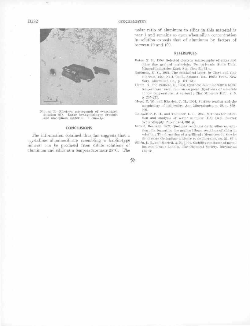
Bl32 GEOCHEMISTRY

FIGURE 3.-Electron micrograph of evaporated solution 2D. Large hexagonal-type crystals and amorphous material. 1 cm=4!-L.

CONCLUSIONS

The information obtained thus £ar suggests that a crystalline aluminosilicate resembling a kaolin-type mineral can be produced £rom dilute solutions o£ aluminum and silica at a temperature near 25°C. The

molar ratio o£ aluminum to silica in this mater ial is near 1 and remains so even when silica concentration in solution exceeds that o£ aluminum by £actors o£ between 10 ·and 100.

REFERENCES

Bates, T. F ., 1958, Selected electron micrographs of clays and other fine grained materials: Pennsylvania State Univ. Mineral Industries Expt. Sta. Circ. 51, 61 p.

Gastuche, l\1. C., 1964, 'l'he octahedral layer, in Clays and clay minerals, 12th Nat!. Conf., Atlanta, Ga., 1963: Proc. , New York, Macllllillan Co., p. 471-493.

Benin, S., and Caillere, S., 1963, Syn'these des mineraux a basse temperature: essai de mise au point [Synthesis of minerals at low temperature: A review] : Clay Minerals Bull. , v. 5, p. 265-271.

Hope, E . W., and Kittricl, , J. H. , 1964, Surface tension and the morphology of halloysite: Am. Mineralogist, v. 49, p. 859-966.

Rainwater, F. H., and Thatcher, L. L., 1960, Methods for collec­tion and analysis of wa'ter samples: U.S. Geol. Suryey Water-Supply Paper 1454, 301 p.

Siffert, Bernard, 1962, Quelques reactions de Ia silice en solu­tion: La formation des argiles [Some reactions of silica in solution: The formation of argillites] : l\Iemoires du Service de al carte Geologique d'Al sace et de Lorraine, no. 21, 86 p.

Silh~n. L. G .. and l\Iartell , A. E., 1964, Stability constants of metal­ion complexes : London , 'l'he Chemkal Society, Burlington Honse.

GEOLOGICAL SURVEY RESEA:RCH 1967

REFERENCE SAMPLE FOR DETERMINING THE ISOTOPIC COMPOSITION OF

THORIUM IN CRUSTAL ROCKS

By j. N. ROSHOLT, JR., Z. E. PETERMAN, and A. j. BARTEL, Denver, Colo.

Abst,·act.-A natural-occurring reference sample has been obtained thnt is belieYed to be in radioactive equilibrium and to hnve n U/~rh ratio similar to 'that of most crustal rocks. The reference sample is t~sed to compare the Th230/Th= activity rntios determined in crustal rocks and to establish the condition of rndionctive equilibrium of Th230 to U238 or Th230 to U:l3-l in these rocks, on the basis of their Th230 /Th= and U238/Th:J3~ con­tent. The mliturul reference sample is u portion of a drill core from n depth of 7,300 feet, nbout 80 feet below the top of the Precnmorinn basement complex, in southwesten1 Saskatchewan, Cnnadn. The roc){, a porphyritic biotite grandte, contains 24.1.±0.2 Pl}m of nrnninm and 82.8±0.9 ppm of thorium.

In the study of geochemical processes involved in the migration of uranium and its isotopes (U23

\ U 23S, U 238)

in the hydrologic cycle, the natural daughter-product tracers (Th230 as a tracer of U 234 and Pa231 as a tracer of U 235

) hn.ve proved quite useful. The amount of ra­dioactive tracer in a rock sa.mple as compared with the amount of radioactive parent isotope present can be determined most accurately by using direct measure­ments of isotopic ratios of individual elements. How­ever, for each element, a reference sample knmvn to be in radioactive equilibrium is required to relate the iso­topic ratios of one element to another in a radioactive decay series.

A National Bureau of Stm1dards reference sample, Hepublic of Congo pitchblende ore (BCP reference), has been used for several years (Rosholt and others, 1963) to determine the isotopic composition of ura­nium. Although the BCP reference is in radioactive equilibrium, it does not contain a sufficient amount of Th232 to permit its use as a suitable.reference for deter­mining the isotopic composition of thorium in crustal rocks. The desirn,ble reference should have a thorium­to-uranium ratio of about 3 or 4; in addition, the U 238-U234-Th230 and the U 235-Pa231 decay sequences should be in radioactive equilibrium.

After comparison of analyses of about 100 granite and volcanic rock sa.mples, most of which do not meet

the criteria of radioactive equilibrium, a porphyritic biotite granite (No. 3633) with a relatively high con­centration of uranium and thorium was selected for the reference. The U 238

- U 234- Th 230 decay sequence is in

equilibrium in the granite, and the Pa231 is presumed to be in equilibrium with U235

• The rock is one of the very few specimens available that meets the criteria for a good reference for thorium isotopes; thus, the signifi­cance and need for such a reference warrants a detailed description of the mineralogy and occurrence of the rock and the method of analysis used to determine its condition of equilibrium.

SAMPLE DESCRIPTION

The sample of biotite granite was obtained from a 3lj2-inch-diameter core of Precambrian basement from the l\fobil Oil Woodley Sinclair Oantuar X-2-21 well in southwestern Saskatchewan, Canada. Precambrian basement was struck at 7,218 feet, and the sample was obtained from the 7,285-7,305-foot interval. The well was drilled on ·an ancient basement high, called the Swift Current nose, which was !a positive feature in Middle Cambrian time (Sawatzky and others, 1960).

Composition

Chemical and modal analyses, and normative min­erals in the sample -are given in table · 1. . . In hand specimen the rock is medium gr.ay, porphyritic, and is characterized by 1nilky-blue phenocrysts of quartz. Textually, the rock has a hypidiomorphic groundmass with a grain size averaging about 0.6 mm. The coarse constituents are euhedral to subhedral phenocrysts of feldspar, up to 15 mm in length, and anhedral ovoidal phenocrysts -of quartz up to 10 mm in length; they make up about 35 percent of the rock. In thin section the blue quartz phenocrysts show marked undulatory extinction with some fracturing. Microcline is un­altered, loc<'lllly poikilitic, and contains both vein and

U.S. GEOL. SURVEY PROF. PAPER 575-B, PAGES B133-Bl36

B133

B134 GEOCHEMISTRY

TABLE !.-Composition of the granite reference sample (No. 3633)

[Sample location: Legal subdivision 2, sec. 21, T. 16 N., R. 71 W. 3, Saskatchewan]

Chemical analysis 1 (weight percent)

Si02--------­AbOa-------­Fe20a--------FeO ________ _ MgO _______ _ Cao ________ _ Na20 ____ - ---K20--- -- -- - -H20+--- - - - --H2o-_______ _ Ti 02 - - - ____ -P205---------MnO _______ _

C02- --- -- - - -Cl __ - - - ____ _ F __________ _

SubtotaL __ Less 0 ____ _ TotaL ____ _

71. 96 12. 73

. 53 3. 17

. 44 l. 37 2. 80 5. 67

. 41

. 02

. 40

. 07

. 06

. 01

. 05

. 30 99. 99

. 14 99. 85

Modal analysis (volume percent)

Quartz _________ 41 Microcline ______ 31 Albite (An 7)---- 20 Biotite_________ 7. 7 Epidote_ _ _ _ _ _ _ _ . 8 Allanite________ . 6 Hornblende___ _ _ . 3 Magnetite______ . 3 Zircon _________ Tr . Apatite ________ Tr . Fluorite________ Tr . Chlorite________ Tr . Sericite_________ Tr. Carbonate______ Tr .

1 Analyst: George 0. Riddle, U.S. Geological Survey. 2 Mesonorm calculations according to Barth (1959, 1962).

Mesonorm 2 (mole percent)

Q ______ 29.98 Or_ _ _ _ _ 29. 48 Ab ____ 25. 75 An____ 5. 15 c______ . 14 BL____ 7. 87 TL____ . 84 Mt_ _ __ . 55 Ap____ . 13

patch-type perthitic intergrowths. Plagioclase (An1) is moderately altered to sericite. The m!afic minerals -biotite, magnetite, epidote, allanite, and hornblende -commonly are clustered together. Some of the allanite has well-developed coronas of euhedral epidote.

Mineralogically the rock is a granite or quartz mon­zonite, depending on the classification used. The lack of agreement between the modal analysis and the norma­tive minerals (table 1) is in part due to the porphyritic texture of the rock and the difficulty in obtaining a representative thin section. Probably for the essential minerals the norm is a more realistic estimate than the mode. The chemical composition of the rock is similar to the composition of Nockolds' (1954) average biotite granite, but the rock contains more FeO and slightly less SiOz.

Regional geology

The Precambrian basement from which the sample was cored is part of the subsurface continuation of the Churchill geologic province of the Canadian Shield (Burwash and others, 1962), which was strongly affected by the Hudsonian orogeny 1.65 to 1.85 billion years ago. Microcline from the biotite granite was dated at 1.66-+-0.08 b.y. by the Rb-Sr method (Peter­man and Hedge, 1964). An indication of a subsequent event is suggested by a K-Ar age of 1.20 b.y. on biotite from the same sample (Burwash and others, 1962). Similar discordant ages were obtained on a~ porphyritic rhyolite from an adjacent well. Hornblende from the rhyolite was dated at 1.49 b.y. (Burwash and others,

1962), whereas the total rock was dated by the Rb-Sr method at 1.71-+-0.19 b.y. The area has probably not been affected by thermal events since Precambrian time.

PROCEDURES

Uranium and thorium concentration

A microsplitter was used to obtain separate samples for determining the uranium and thorium concentra­tion; the technique of isotope dilution was used for these analyses (Rosholt and others, 1966). A U235

spike and a Th230 spike were added from a combined spike solution to a 0.5-gram sample in HN03 in a Teflon dish. The sample was decomposed with HF, HN03, and HCl04, and evaporated to dryness in nitrate form. The sample in 6N HN03 solution was loaded on an anion exchange column (NO; form), w.ashed with 6N HN03, and thorium and uranium were eluted with 0.5N HCl. The eluate was repurified by anion exchange in a similar manner on a smaller column. The sample was evaporated to dryness with one drop of HOl04 and HN03 mixture to destroy any organic matter, and then was loaded on the multiple filament for mass-spectrometry measurement of ura­nium and thorium isotopes.

.Isolation of uranium and thorium

A 2-g sample was decomposed by HN03, HF, and HOI04 in a 400-milliliter Teflon dish. A 20-g sample was also used to test the isolation of uranium and thorium from a larger sample than actually required for analysis. The insoluble residue remaining after acid decomposition was removed by centrifugation or filtration from a 6N HOI solution. The solution was loaded on an anion exchange column (Ol-1 form), washed with 6N HOI, and uranium was eluted with 0.5N HOI. The .eluant and chloride washmgs were retained for isolation of thorium. The eluate was converted to nitrate form, approximately 50 ml of saturated Al(N03)a solution was added for a salting­out agent, and uranium was extracted into hexone. Uranium was back-extracted from hexone with H20 and reextracted with hexone, using NH4N03 for a salting-out agent. The purified sample was loaded on multiple filaments for mass-spectrometric measure­ments.

Isolation of thorium

The eluant from the chloride anion exchange column was converted to nitrate by successive evaporation with 6N HN03. The solution was loaded on an anion exchange column (N031 form), washed with 6N HN03

and eluted with 0.5N HOI. A second anion exchange separation was made using a smaller column. To com­pletely remove uranium from thorium, the eluant was

ROSHOLT, PETERMAN, AND BARTEL Bl35

converted to chloride form, passed through a small column (Cl-1 form), and washed with 6N HCl. The purified solution, in which thorium isotopes were in­cluded together with the wash solution, was evaporated to dryness with one drop of HC104 in a 10-ml Teflon beaker. A thin source of thorium for alpha spectrom­etry measurement was prepared by electroplating from a 2N NH4Cl solution (pH 6) at 6 volts and 0.4 ampere for 1~ hours.

Isotopic measurements

The mass spectrometric and alpha spectrometric measurements used were the same as those described by Rosholt and others (1966). For a minimum sta­tistical variation, a large number of. counts were ob­tained on the alpha spectrometer measurements. Ap­proximately 70,000 counts of Th232 were obtained for each of 4 different sample splits for Th230/Th232 ratios, and approximately 60,000 counts of U238 were obtained for each measurement of the U234jU238 ratios.

R·ESULTS

The results of these analyses are shown in table 2; uranium content is 24.1 ±0.2 parts per million, and thorium content is 82.8±0.9 ppm. The U/Th ratio has less analytical variation than the actual concen­trations of these elements because, using a combined spike, any variation in the weight of the spike produces the same variation for each element. Variation of the U/Th ratio in any individual analysis did not exceed 0.4 percent of the average value.

The isotopic ratios U238/U235, U235/U23

\ U238JU23\ and

Th 230 j'I'h 232 are shown in table 3. No analytically significant variation of the U238jU235 ratio was measured, and the U235jU234 ratio indicates that U234 is less than 0.5 percent deficient compared to U238 or U235

•

TABLE 2.-Uranium and thorium concentration, in parts per million, determined by isotope dilution, and U /Th weight ratio of the granite reference sample (No. 3633) '

Sample split u '.rh

5 ____________________ 23. 9.1 81. 99 6 ____________________ 24. 45 84. 28 7 ____________________ 23. 98 82. 20

Average ________ - - - __ 24. 1 82. 8

Standard deviation ____ ±0. 2 ±0. 9

u 'J'h

0. 2916 . 2901 . 2917 . 2911

--------

0. 2894 . 2880 . 2896 . 2890

±0. 0008

The equation for the calculation of the unity reference ratio of 'thorium isotopes is given in table 3; unity reference is the ratio of the activity of Th230, in equilib­rium with 1 ppm of U238

, to the activity of 1 ppm of Th232

• This reference ratio is used for comparison with the measured Th230/Th232 activity ratio determined on rock samples for which the Th230jU238 relation is sought. Division of the Th230/Th232 activity ratio of a sample by the unity reference ratio is made so that a direct comparison can be made with the U238/Th232 concentra­tion ratio in the sample. Thus,

Th230/Th232 (sample) Th230/Th232 (unity ref.)

equivalent Tlr30 (ppm) Th232 (ppm)

(sample).

The right-hand term of the equation is an equivalent weight-to-weight ratio which· can also be defined as the amount of U238

, in parts per million, that would be required to support, in radioactive equilibrium, the measured amount of Th230 for each part per million of thorium in the sample. Thus, any activity ratio will yield an equivalent weight ratio after comparison with the reference. In the comparison of the Th230 (equiv.)/ Th232 weight ratio with the U238/Th232 weight ratio,

TABLE 3.-Isotopic composition of 11.mniurn and thorium, and Th230/Th232 reference value of the granite reference sample (No. 3633)

Mass spectrometric determination Alpha spectrometric determination

Sample split U23B/Um (BCP ref.)

U23SfU23& (granite) U23&fU234 (BCP ref.)

U23&/U234 (granite) U239/U234 (BCP ref.)

U23BfU234 (granite) Th230fTh232 (granite)

(activity ratio)

------------------------ ------------ --------·-------1---·--·--------------- -----------

1_ - - - - - - - ----- - - - - - - - - - - - - - - - - - - - - 1. 001 0. 995 - - - - - - - - - - - - - - - - - - - -2_________________________________ 1. 001 . 999 0. 995

:3- - ----- - - - - - - - - - - - - - - - - - - - - - - - - - - . 998 . 998 . 999 4--------------------------------- -------------------- -------------------- --------------------

Th2so . . . u2as . . Th232 (act1v1ty rat1o) = 0.870± 0.008; Th232 (weight ratio)= 0.2890± 0.0008.

Th2so . Th230/Th232 (activity ratio) 'fh232 (umty reference)

1 u2as;Th2a2 (weight ratio)

0·870 3 0 0 03 0.289= . l± . .

0. 8872 . 8719 . 8561 . 8649

• Hatio or tho alpha radioactivity or 'J'h23o, in equilibrium with 1 ppm or u2as, to the alpha radioactivity of 1 ppm of Th232. Unity reference is used for the following comparison:

nnd for rock sample:

Th230/Th232 (sample) equivalent Th230 (ppm) 'l'h23°/'l'h232 (unity ref.) 'J'h232 (ppm) (sample)'

'L'h230 equiv. 'l'h23o (ppm)/Th232 (ppm) U23S (activity ratio) U238 (ppm)/Th232 (ppm)

Bl36 GEOCHEMISTRY

values of the former ratio that are greater than the U238jTh232 ratio indicate an excess of Th230 compared with U238

•

An additional check of equilibrium conditions of the granite reference can be made by comparing the unity reference ratio with the value that would be obtained from the decay constants of U238 and Th232

• Using 4.51 X 109 years for the half life of U238 (Fleming and others, 1952) and the adopted "best" value (Hyde and others, 1964, p. 489) of 1.39 X 1010 years for the half life of Th232 (Kovarik and Adams, 1938; Picciotto and Wilgain, 1956), a unity reference ratio is calculated by the following equation:

x_238N23s

x. ?.32N232 3.01,

where X. is the decay constant and N is the number of atoms. This number is nearly identical with the value in table 3 measured for the reference sample (No. 3633).

Barth, T. F. ,V., 1959, Principles of classification and norm calculations of metamorphic rocks: Jour. Geology, v. 67, no. 2, p. 135-152.

--- 1962, A final proposal for calculating the mesonorm of metamorphic rocks: Jour. Geology, v. 70, no. 4, p. 497-498.

Bm·wash, R. A., Baadsgaard, H., and Peterman, Z. E., 1962, Pre­cambrian K-Ar dates from the western Canada ,sedimentary basin: Jour. Geophys. Research, v. 67, no. 4, p. 1617-1625.

Fleming, E. H., Jr., Ghiorso, A., and Cunning-ham, B. B., 1952, The specific alpha-activities and half-lives of U234

, un", and U238

: Phys. Rev., v. 88, p. 642. Hyde, E. K., Perlman, I., and Seaborg, G. T., 1964, The nuclear

properties of the heavy elements, v. 2, Detailed radioactivity properties: Englewood Cliffs, N.J., Prentice-Hall, Inc., p. 409-1107.

Kovarik, A. F., and Adams, N. 1., Jr., 1938, The disintegration constant of thorium and the branching ratio of thorium-C: Phys. Rev., v. 54, p. 413.

Nockolds, S. R., 1954, Average chemical compositions of some igneous Tocks: Geol. Soc. America Bull., v. 65, p. 1007-1032.

Peterman, Z. E., and Hedge, C. E., 1964, Age of basement rocks from the 'Villiston basin of North Dakota and adjacent areas: Art. 141 'in U.S. Geol. Survey Prof. Paper 475-D, p. D100--D104.

Picciotto, E., and 'Vilgain, S., 1956, Confirmation de la periode du Thorium-232: Nuoro Cimento, ser. 10, v. 4, p. 1525-1528.

Rosholt, J. N., Jr., Doe, B. R., and Tatsumoto, 1\I., 1966, Evolu­tion of the isotopic composition of uranium and thorium in soil profiles: Geol. Soc. America Bull., v. 77, p. 987-1004:

Rosholt, J. N., Jr., Shields, 'V. R., and Garner, E. L., 1l)63, Isotopic fractionation of uranium in sandstone: Science, Y. 5.9, p. 224- ·226.

Sawatzky, H. B .. Agarwal, H. G., and Willson, ,V., 1960, Helium prospects in southwest Saskatchewan: Saskatchewan Dept. Mineral ReSDurces Rept. 49, 26 p.

GEOLOGICAL SURVEY RESEARCH 1967

GEOCHEMISTRY OF DEEP-SEA SEDIMENT

ALONG THE 160° W. MERIDIAN IN THE NORTH PACIFIC OCEAN

By VERNON E. SWANSON, JAMES G. PALACAS, and ALONZA H. LOVE, Denver, Colo.

Work done in cooperation with the U.S. Coast ana Geoaetic Survey

A.bstract.-The lithology and chemical composition of the upper 25 em of light-brown clay are remarkably uniform along the 2,000-mile traverse from southern Ala·ska to the Hawaiian Islands, except for the olive-gray color and relatively higher organic matter content of the Aleutian Trench sample. Six of seven shnllow cores contained ice-rafted pebbles, most of which have n thin ferromanganese coating. .Analyses of sediment show little variation from the average content of 0.21 percent organic carbon, 0.05 percent nitrogen, 85 ppm of soluble humic fraction, nnd 45 ppm of soluble bitumen. fraction. The exception is the Aleutian Trench sediment, which contains about 0.5 percent organic carbon; and 590 ppm of soluble humic frac­tion. The nverage pH of the upper 2-3 em of sediment of all the cores of the traverse is 7.2, compared to 7.9 for the im­mediately overlying water; the average Eh of the sediment is +259 mv, compared to +182 mv for the water.

This report is based on core samples obtained by the U.S. Coast and Geodetic Survey oceanographic ship S~t'rveyo1· during its cruise from Alaska to Hawaii in September 1964. The seven coring stations are located along the 160° W. meridian from about 150 miles south of the Shumagin Islands at the eastern end of the Aleutian chain, southward to a few hundred miles north of the Hawaiian Islands (fig. 1, table 1). Four of the cores were obtained with a steel box corer (8 X 8 X 15 inches) which was constructed aboard ship. This large but shallow-penetration corer pro­vided sufficiently large volumes of sediment to conduct a variety of chemical analyses, particularly those re­quired to characterize the organic matter in the sedi­n1ents. Three cores were obtained with a Phleger cor­er, but sediment samples from cores C3 and C5 (table 1) were not made available for chemical analysis. In this report the cores are labeled as follows : BC, box core (collected on the S~t'l'veyor 1964 cruise) ; d, Phle­ger or modified-piston core (collected on the Surveyo1·

1964 cruise) ; P, Pioneer ( 1963) core. Individual sam­pies of certain cores are labeled in lowercase letters (as for example, BC2a, 2b, and so forth).

This study of the uppermost, most recently de­posited, deep-sea sediment from the North Pacific is aimed at determining sediment composition, partic­ularly the contained organic material, and •at adding to our know ledge about the geochemical processes ac­tive near the sediment-water interface. The results are related to similar studies on older and deeper ·parts of other North Pacific cores (Palaoas and others, 1966), and to studies in progress on Atlantic continen­tal-shelf sediments and bay sediments from the Atlan­tic and Gulf of Mexico coasts.

The senior author, who was aboard ship, acknow­ledges with gratitude the advice and assistance of the crew of the s~trveyor in obtaining the cores, especially Capt. Don A. Jones, Comdr. J.D. Boyer, Comdr. R. G. Metcalf, Lt. Comdr. S. M. Levine, Chief Surveyor Tech. Dudley Doe, and Chief Engineer Tech. Peterson. The cooperation of T. V. Ryan, N. P. Laird, and W. A. Anikouchine, of the U.S. Coast and Geodetic Survey, and of Thomas A. Hendricks and George W. Moore, of the U.S. Geological Survey, also is greatly {t:ppre­ciated.

PROCEDURES

Immediately after the cores were hoisted aboard the S~urveyor, pH, Eh, and temperature measurements were made, and the core material was divided into sample interv·als. The pH and Eh determinations (table 1) were made with a portable pH meter on small samples of the water trapp~d in the corer just above the sediment and of the uppermost 2-3 centi­meters of the sediment itself. Most of these samples were obtained from a Phleger corer, which was used

U.S. GEOL. SURVEY PROF. PAPER 575-B, PAGES B137-Bl44

B137

Bl38 MARINE . GEOLOGY

130° 120° 110°

BC4

eP105

Hawaiian

20ot-----l-----1--<::>w-::::;·0~Is_Ia_nd_s-l----+----r

FIGURE 1.-Map showing position of core stations in North. Pacific Ocean. BC, box core, and C, Phleger or modified­piston core, Surveyor (1964). P, Pioneer (1963) core ( Palacas and others, 1966).

as the tripping weight for the box corer or a large piston corer, so that the sediment in the larger corers was not disturbed.

The pH meter was standardized and checked with appropriate buffer solutions, both before and after measurement of a sample. A reading was recorded immediately on inserting the instrument probes into the sample, and· another reading was recorded after 30 seconds, both corrected for temperature. The pH and Eh readings given in table 1 are those taken after 30 seconds, at which time equilibrium conditions were generally attained, as indicated by negligible needle­drift on the instrument. The precision of these values is probably +0.1 pH unit and + 10 millivolts Eh.

No stratification was observed in any of the short cores (7.5-34.5 em) described in this report, so sa·mple

interv·als of generally 3 or 6 em were arbitrarily chosen. The core samples were frozen ·in the ship's food locker, and kept frozen to minimize bacterial de­cay and oxidation until they were analyzed. General description of the sediment in the cores was made at time of collection, and small representative fractions of the samples were later examined for gr·ain size, tex­ture, color, mineralogy, and fossil content ..

All sample preparation and analytical methods em­ployed in the laboratory are the same as those described by Palacas ·and others ( 1966, p. 0103) for the Pionee'l' ( 1963) cores, with the following exceptions :

The soluble humic fraction was extracted with 0.1N NaOH in two steps by ultrasonic agitation for 5-10 minutes; the step of shaking on a mechanical shaker for 8-10 hours was omitted as unnecessary. Organic­nitrogen analysis of the sediment was substituted for amino-acid analysis with the intent of providing a somewhat broader and more easily obtained organic geochemical parameter. Percentage of nitrogen was determined in duplicate by micro-Kjeldahl analysis slightly modified after McKenzie and Wallace ( 1954) .

pH, Eh, AND TEMPERA:TURE OF BOTTO·M WATER AND SEDIMENT

All the deep bottom waters and bottom sediments described are slightly alkaline and oxidizing, which is typical of most oceans. From a geochemical view­point, significant differences in pH and Eh exist be­tween the water ·and the sediment (table 1) . The pH of the uppermost sediment is invariably lower than that of the overlying water ·at each station; the Eh is, with one exception ( 04, table 1), higher in the sedi­ment than in the overlying water. The pH and Eh measurements do not, however, indicate major chem­ical differences between environments of sedimentation, such as one might suspect between the Aleuti·an Trench ( B01) and the North Pacific abyssal plains to the south ( B02-4) .

TABLE I.-Geographic position of cores and measurements taken at each sample station

[BC, box core; C, Phleger or modified-piston core]

Depth of water Bottom-water Upper-sediment SURVEYOR measurements measurements

Core designation station and Coordinates sample Nos.

(m) (ft) pH Eh (mv) pH Eh (mv) --------------------

BC L ___________ S-18-64 53°11.4' N., 161 °54.0' W. 6,670 21, 883 8. 24 +175 7. 02 +272 C3 _____________ S-19-64 50°51.3' N., 161 °08.1' W. 5,020 16, 470 7. 78 +194 7. 30 +257 C4 _____________ S-20-64 48°18.1' N., 160°47.9' W. 5,060 16,602 7. 73 +203 7. 52 +179 BC2. ___________ S-21-64 47°19.0' N., 160°45.0' W. 5,090 16,699 7. 91 +160 7. 18 +247 C5 _____________ ~-22-64 45°02.0' N., 160°39.0' W. 5,300 17,388 7. 52 +179 7. 27 +295 BC3 ____________ ---------- 39°25.5' N., 160°24.8' W. .5, 273 17,300 7. 75 +185 7. 10 +311 BC4 ____________ S-23-64 28°32.8' N., 159°59.0' W. 6, 050 19,849 8. 15 +181 7. 27 +255

SWANSON, PALACAS, AND LOVE B139

The average pH of the upper 2 em of sediment is 7.2, but the average pH of the sea water a few centi­meters ·above the sediment is 7.9. These data are very similar to those reported by Emery and Rittenberg ( 1952, p. 7~69) on 21 deep-sea cores from the central east Pacific; the topmost sediment of these cores had an average pf.I of 7.40 as compared with 7.85 for the overlying water. The difference in pH between the sediment and the overlying water has been explained by Siever and others ( 1965, p. 65) as being a result of bacterial oxidation of organic matter in the sedi­ment, which causes buildup of CO 2 and lowers the pii. Actually, as Moore and others ( 1962) deter­mined, the C02 content of North Pacific deep-sea sediment is indeed several times greater than that of the overlying water, which they ·attributed to decay of orgn.nic material within the sediment.

The average Eh of the water is + 18.2 Inv, and that of the sediment is + 259 mv, suggesting that the bot­tom sediment is slightly more oxidizing than the over­lying water. This relation is just the opposite of that observed in the marine basins off southern California (Emery and Rittenberg, 1952, figs. 6-17), where the sediments contain generally 10 times more organic rnatter than the North Pacific cores.

All the pH and Eh data, including the information recorded by Moore and others (1962, tables 33.1, 33.2), suggest continuous circulation of bottom water in most of the North Pacific Ocean. Furthermore, the amounts of organic m·atter in the sediment, as de­scribed ]ater in this report, are apparently too small to produce the acidic and reducing conditions charac­teristic of the bottom water and sediment in some marine environments.

The temperature of all water and sediment samples, as men.sured immediately after collection, was about 1 °C, which is common throughout the world at the ·depths these samples were collected.

DESCRI'PTION OF SED:IMENT

Most of the sediment in the cores is typical oceanic abyssal clay-more descriptively, a tan to light-brown 1utite. The detailed descriptions of the sediment in the samples that have been chemically analyzed are given in table 2, and the relative amounts of different minerals in these samples, as determined by X-ray diffraction analysis, are listed in table 3.·

Ferromanganese nodules and grains are common in many bottom-sediment samples from the Pacific Ocean (1\tienard, 1964, fig. 8.3), but none of the Surveyor (1964) cores reported here contained more than a few isolated grains or thin ferromanganese crusts on pebbles.

241-334 0-07--10

TABLE 2.-Description of sediment from North Pacific cores

[BC; box core; C, Phleger or modified-piston core]

Core

BCl (7.5 em)

C4a (6.0 em)

C4b (7.0 em)

BC2 (34 . .5 em, total)

BC2a (3.0 em, top sample)

Description

Clay, olive gray (5 Y4/1) when wet, light olive gray (5Y6/1) when dry; gummy and very cohesive when wet; about 5 percent biogenic material, diatoms abundant, few globular Radiolaria, few spines, and some brownish claylike fecal pellets;<5 percent fine sand, includes rock fragments of basaltic ash, reddish and yellowish chert, angular quartz, and few glass shards; heavy minerals not common; no visible stratification.

Silty clay, grayish brown (5 YR3/2) when wet, moderate yellowish brown when dry; somewhat spongy; abundant diatoms of variable size, some globular Radiolaria, few Foraminifera, and few spines and spicules; about 5 percent angular rock fragments as much ~ts 1 em across, and very fine sand consisting of about 25 percent dark minerals; sharp contact with unit below.

Silty clay, light olive gray (5 Y5/2) when wet, yellowish gray (5Y7/2) when dry; fossils as abov~, with few fish bone fragments; about 10 percent sand of variable grain size, angular to subrounded grains and fragments of quartz, basalt, chert, mica, and serpentine(?); magnetic minerals un­common; about 5 percent angular to sub­rounded rock fragments as much as 1.3 em across.

Silty clay, dark yellowish brown (10YR4/2) when wet, pale yellowish brown (10YR6/2) with slight greenish hue when dry; no apparent stratification; silt, sand, and gravel of highly variable composition scattered throughout; pebbles, as much as 2.7 em in diameter, make up as much as 10 percent, and sand and silt make up from a few to 5 percent; coarse fraction decreases in size and abundance down­ward; 10 to 40 percent biogenic material, with abundant diatoms, fairly abundant Radiolaria, spines common, very few Foraminifera, and some miscellaneous fossil types.

As above, poorly sorted, about 10 percent sand and gravel; fairly abundant pebbles, 2.7-cm maximum dimension, angular to subrounded, partly crusted with ferro­manganese, largely rock fragments includ­ing sandstone, quartzite, chert, basalt, and diorite; sand includes rock fragments n.nd grains of olivine, epidote, pyroxene or hornblende, feldspar, muscovite, quartz, and some magnetite and ilmenite; about 20 percent siliceous skeletal material, small diatoms (60 percent), Radiolaria (25 percent), spines (5 percent), and a few Foraminifera, tubes, and unidentified material.

B140 MARINE GEOLOGY

TABLE 2.-Description of sediment from North Pacific cores-Con

[BC, box core; C, Phleger or modified-piston core]

Core

BC2b (3.0 em)

BC2c ~3.0 em)

BC2d (3.0 em)

BC2e (3.0 em)

BC2f (3.0 em)

BC2g (16.5 em, bot~om sample)

BC3 (20 em)

BC4 (22.5 em, total)

BC4a (6.0 em, top sample)

Description

Very similar to sample 2a except slightly less coarse material; pebbles slightly smaller, maximum of 1.6 em across, with one flat siltstone chip 1.2 em across, and small mollusk shell fragment.

Very similar to sample 2a, but only .5-7 per­cent sand and gravel; magnetite slightly more abundant; some larger diameter diatoms.

Similar to samples 2a-c, but overall grain size smaller, and sand fraction better sorted; angular quartz and feldspar more abundant; maximum pebble diameter 0.4 em; diatoms relativ!Jly more abundant; chitinous shell of Orbiculoidea-type brachi­opod, 2. 7 mm diameter.

Similar to samples 2a-d, with somewhat less coarse material; very few small pebbles; about 40 percent of sediment is diatoms, mainly larger diameter type.

Similar to sample 2d; coarse fraction less than 5 percent, mostly quartz and feldspar grains and includes very few small pebbles, maximum diameter 0.2 em; diatoms abundant.

Similar to sample 2f; glass shards fairly abundant; diatoms abundant.

Clay, moderato yellowish brown (l.OYR5/4) when wet, grayish orange (lOY R7/4) when dry; slightly plastic; about 5 percent bio­genic material, mainly Radiolaria, spines common, few diatoms, and a few un­identified fragments; scattered rock gran­ules, subrounded to angular, 0.1-0.4 em in diameter, mainly basalt, but also diorite quartzite, partly coated and stained by a very thin ferromanganese crust; about 3 percent very fine sand, mainly quartz, some magnetic grains, and a few glass shards; no visible stratification.

Clay, dark yellowish brown (10YR4/2) when wet, pale yellowish brown (10YR6/2) when dry; upper 6 em very sticky and gummy ·when wet, somewhat crumbly below 6-cm depth; stratification below 6-cm depth caused by several brownish-black laminae containing disseminated fine- and medium­size grains of basaltic ash; few Radiolaria, some siliceous spines, scattered small fish­teeth, and bone fragments; a few ferro­manganese and phosphatic(?) grains.

As above, nonclay material <2 percent; fish teeth 0.1-.25 mm long common; few globular Radiolaria, needle-shaped, branch­ing, and tetrapod spines, few minute bone fragments; few ferromanganese grains, reniform and botryoidal surfaces, 0.1-1. 0 mm in diameter; yellowish phosphatic(?) grains, semitranslucent, 0.1-0.5 mm in diameter.

TABLE 2.-Description of sediment from North Pacific cores-Con.

[BC, box core, C, Phleger or modified-piston core] Core

BC4b (6.0 em)

BC4c t10.5 em, bottom sample)

Description

Similar to 4a, except grains or fragments of basaltic ash more common but <5 percent of sample; grains are dark gray, sub­rounded, 0.1-0.5 mm in diameter, and have spongy structure; biogenic material similar to 4a except broken spines and teeth common.

Similar throughout to sample 4b.

The most notable characteristic of the bottom sedi­ment is the inclusion of pebbles, granules, and sand in the clay of all except the southernmost core (BC4). Although gravel can be transported to the deep sea by many mechanisms (Emery, 1963), the variable size, shape, and mixture of rock types support the interpretation that the coarse material was ice rafted from the north, to at least as far south as 39°25.5' N., about the latitude of Denver, Colo. The coarse ma­terial, which rarely made up more than 5 percent of the total sediment, w:as excluded frmn the samples chemically analyzed.

The gravel was present to a depth of at least 34.5 em (BC2), but became less abundant with depth. All pebbles were at least partly coated with a thin ferro­manganese crust; some pebbles apparently had been partly buried in the clay, and only their upper exposed parts were coated by precipitating ferromanganese.

Thin sections of 6 pebbles from the upper 9 em of BC2 were studied under a polarizing microscope. The 6 angular to subrounded pebbles ranged from 1.4 to 4.4 em in maximum diameter and were identified as follows: gabbro, porphyritic basalt, metamorphosed quartz diorite, poorly sorted quartzite, feldspathic mudstone, and dolomitic limestone.

No unusual biogenic material was observed in the cores. Lacy, siliceous, skeletal remains of diatoms and Radiolaria, and transparent siliceous spines are com­mon in all samples. The few Foraminifera were found only in BC2 and 4 ( taJble 2; fig 1). Minute conical fishteeth, many of them broken, were relatively abundant in BC4, and a few bone fragments were observed in all cores.

CHEMICAL COMPOSITION OF SEDIMENT

In general, the chemical composition of all samples is remarkably uniform, as shown by the narrow ranges of element contents in truble 4. With the ex­ception of minor differences in amounts of magnesium, calcium, and potassium, none of which show geo­graphic or stratigraphic trends, there are no notable differences in major-element composition.

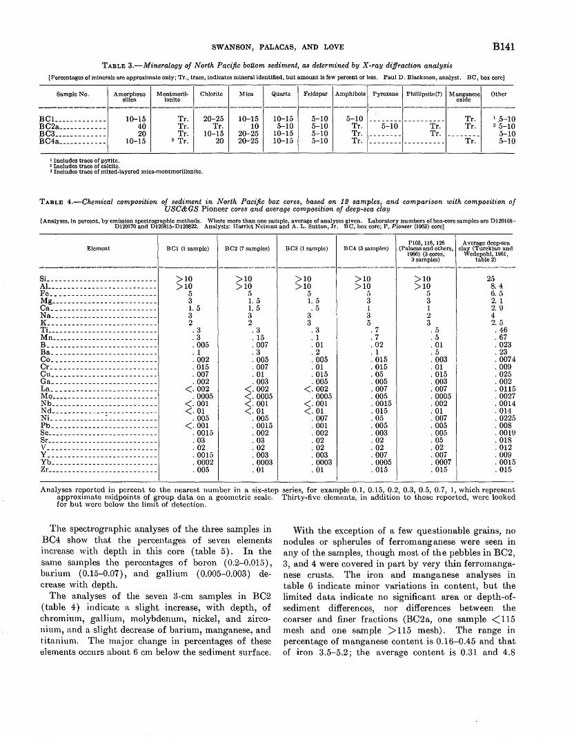
SWANSON, PALACAS, AND LOVE Bl41

TABLE 3.-Mineralogy of North Pacific boUom sediment, as determined by X-ray diffraction analysis

[Percentages or minerals are approximate only; Tr ., trace, indicates mineral identified, but amount is rew percent or less. Paul D. Blackmon, analyst. BC, box core]

Sample No. Amorphous Montmoril- Chlorite Mica Quartz Feldspar Amphibole Pyroxene Phillipsite(?) Manganese Other silica lonite oxide

----------- ----------------- __ ..,. __ ----- ------ ---------- ----·------------BCL ____________ BC2a _______ -----BC3 _____________ B C4a ____________

I Includes trace or pyrite. ~ Includes trace or calcite.

1Q-15 40 20

10-15

Tr. Tr. Tr.

3 Tr.

3 Includes trace or mixed-layered mica-montmorillonite.

2Q-25 10-15 1Q-15 Tr. 10 5-10

10-15 20-25 10-15 20 2Q-25 1Q-15

5-10 5-10 -------- ---------- Tr. I .5-10 5-10 Tr. 5-10 Tr. Tr. 2 5-10 5-10 Tr. -------- Tr. -------- 5-10 5-10 Tr. -------- ---------- Tr. 5-10

TABLE 4.-Chemical composition of sediment in North Pacific box cores, based on 12 samples, and comparison with composition of USC&GS Pioneer cores and average composition of deep-sea clay

[Analyses, in percent, by emission spectrographic methods. Where more than one sample, average or analyses given. Laboratory numbers of box-core samples are Dl20168-Dl20170 and Dl20815-Dl20822. Analysts: Harriet Neiman and A. L. Sutton, Jr. BC, box core; P, Pioneer (1963) core]

Element

Si __________________________ _ AI __________________________ _ Fe _________________________ _

~ag::======================== ~a--------------------------1{ __________________________ _ Ti __________________________ _

~n--------------------------B __________________________ _ Ba _________________________ _ Co _________________________ _ Cr _________________________ _ Cu _________________________ _ Ga _________________________ _ La _________________________ _

~0--------------------------~b _________________________ _

~ d_--- - --- - - .. - -- - - - ---- - - ---~i _____________ :~-----------Pb _________________________ _ Sc __________________________ _ Sr __________________________ _

''---------------------------y __________________________ _ Yb _________________________ _ Zr __________________________ _

BCl (1 sample)

>10 >10

5 3 1.5 3 2 .3 .3 . 005 . 1 . 002 . 015 . 007 . 002

<· 002 . 0005

<· 001 <· 01 . 005

<· 001 . 0015 . 03 . 02 . 0015 . 0002 . 005

BC2 (7 samples)

>10 >10

.5 1.5 1.5 3 2 .3 . 15 . 007 .3 . 005 . 007 . 01 . 003

<. 002 <. 0005 <. 001 <. 01 . 005 . 0015 . 002 . 03 . 02 . 003 . 0003 . 01

BC3 (1 sample)

>10 >10

5 1.5 .5

3 3 .3 . 1 . 01 .2 . 005 . 01 . 015 . 005

<. 002 . 0005

<. 001 <. 01 . 007 . 001 . 002 . 02 . 02 . 003 . 0003 . 01

BC4 (3 samples)

>10 >10

5 3 1 3 5 .7 .7 . 02 . 1 . 015 . 015 . 05 . 005 . 007 . 005 . 0015 . 015 . 05 . 005 . 003 . 02 . 02 . 007 . 0005 . 015

P105, 116, 126 A vcrage deep-sea (Palacas and others, clay (Turekian and

1966) (3 cores, Wcdepohl, 1961, 3 samples) table 2)

>10 >10

5 3 1 2 3 .5 .5 . 01 .5 . 003 . 01 . 015 . 003 . 007 . 0005 . 002 . 01 . 007 . 005 . 005 . 05 . 02 . 007 . 0007 . 015

25 8. 4 6. 5 2. 1 2. 9 4 2. 5 . 46

.. 67 . 023 . 23 . 0074 . 009 . 025 . 002 . 0115 . 0027 . 0014 . 014 . 0225 . 008 . 0019 . 018 . 012 . 009 . 0015 . 015

Analyses reported in percent to the nearest number in a six-step series, for example 0.1, 0.15, 0.2, 0.3, 0.5, 0.7, 1, which represent approximate midpoints of group data on a geometric scale. Thirty-five clements, in addition to those reported, were looked for but were below the limit of detection.

The spectrographic analyses of the three samples in BC4 show that the percentages of seven elements increase with depth in this core (table 5). In the same samples the percentages of boron ( 0.2-0.015), barium (0.15-0.07), and gallium (0.005-0.003) de­crease with depth.

The analyses of the seven 3-cm samples in BC2 (table 4) indicate a slight .increase, with depth, of chromium, gallium, molybdenum, nickel, and zirco­nium, and a. slight decrease of barium, manganese, and titanium. The major change in percentages of these elements occurs about 6 em below the sediment surface.

With the exception of a few questionable grains, no nodules or spherules of ferromanganese were seen in any of the samples, though most of the pebbles in BC2, 3, and 4 were covered in part by very thin ferromanga­nese crusts. The iron and manganese analyses in table 6 indicate minor variations in content, but the limited data indicate no significant area or depth-of­sediment differences, nor differences between the coarser and finer fractions (BC2a, one sample < 115 mesh and one sample > 115 mesh). The range in percentage of manganese content is 0.16-0.45 and that of iron 3.5-5.2; the average content is 0.31 and 4.8

B142 MARINE GEOLOGY

TABLE 5.-Percentages of seven elements that increase with depth in BC4

[Analyses, in percent, by emission spectrographic method. Laboratory numbers are D120168-D120170. Analyst: A. L. Sutton, Jr. BC, box core]

Sample Elements interval -----------------------------(em)

Co Cu La Mo Ni Pb y

------- -------------------o-6 _______ 0. 01 0. 03 0. 001). o. 0015 0. 03 0. 003 0.003 6-12 _______ . 015 . 05 . 007 . 005 . 05 . 005 . 007 12-22.5 ____ . 02 . 07 . 01 . 007 . 05 . 007 . 01

percent, respectively, for the 4 cores. The presence of these metals in their oxidized state, Mn02 and Fe203, is supported by observations of the sediment under the microscope (table 2), and by the positive Eh (table 1) of the sediment when collected.

Because copper is commonly closely associated with organic matter in carbonaceous sediment, the copper content of the samples was determined (table 6) . The limited analytical data on copper in the sediment show no system:atic increase of copper with increase of or­ganic-matter content. The increase of copper content with depth in BC4, as indicated by the spectrographic analyses (table 5), aotually suggests an inverse corre­lation between copper content and organic matter (see organic-matter :analyses, table 7). The average copper content of the sediment is 0.014 percent, and the range is 0.0078-0.021 percent. The data do show a slight increase in copper content from north to south for the 4 box-core samples (BC1, 2, 3, 4), 78, 96, 190, -and 210 parts per million, respectively, but this relation must be supported by much more data before it can be con­sidered valid.

ORGANIC MATJER IN SEDiiMENT

In the geochemical sense used here, organic matter in sediment includes the tissue of protoplasmic sub­stances of plants and animals, and their decay prod­ucts, that are composed predominantly of carbon, hydrogen, and oxygen, with small amounts of nitro-_

TABLE 6.-Manganese, iron, and copper content of uppermost sediment in North Pacific cores

[Analyses, in percent, by atomic-absorption method. J. D. Mensik, analyst. BC, box core]

Laboratory Sample N?. No.

--------- ------BCL _________ . D12111 7 BC2a 1 ________

BC2a 2 ________

B C2e _________ B C3 ___ - - - - - - -BC4 __________

1 <115-mesh fraction. 2 >115-mesh fraction.

18 19 20 21 22

Thickness of sample

interval (em) ------

7. 5 3. 0 3.0 3. 0

20. 0 6. 0

Mn Fe Cu

----------0. 37 5. 2 0. 0078

. 24 4. 6 . Oll

. 29 3. 5 . 0092

. 16 3. 9 . 0092

. 20 4. 9 . 019

. 45 5. 0 . 021

gen, sulfur, and phosphorus; excluded are the silica, carbonate, and phosphatic material in shells or skele­tons. The nonskeletal organic matter is not visible in the North Pacific sediment and must be determined chemically.

The sediment in the Surveyor cores has been an­alyzed by several methods to characterize the organic matter. The four 'basic determinations are: percent­age organic carbon, percentage nitrogen, percentage soluble humic fraction, and percentage soluble bitu­men fraction. The organic-carbon determination is the best measure of the total organic matter in the sediment. The nitrogen content, as determined by the micro-Kjeldahl method, is in part a measure of the amount of proteinaceous substances in the organic matter. The amount of alkali-soluble humic material, may be indicative of the original biologic material, particularly of woody plant material and some types of algae. The organic matter soluble in benzene is the bitumen fraction :and, although this fraction includes variable amounts of waxes, resins, fats, and oils, it may be considered a measure of the amounts of satur­ated and aromatic hydrocarbons and the asphaltic substances in the sediment. Bordovskiy ( 1965, p. 33~ 114) has presented an excellent summary of the ranges in content and the significance of these chemical com~ ponents of organic matter in Recent marine sediments.

The general range of organic-matter content in North Pacific deep-sea sediment, based on ·analysis of the Surveyor cores, is 0.07 to 0.9 percent, but most commonly the sediment contains 0.2-0.5 percent or­ganic matter. Based on 16 samples from 8 cores, 5 S1trveyor cores (table 7) and 3 Pioneer (1963) cores (fig. 1; Palacas and others, 1966), the deep-sea sedi­ment in the North Pacific contains -an average of 0.4 percent organic matter.

The analytical data on the sequence of samples from BC4 (table 7) suggest a slight decrease in amount of organic matter with depth of sample. This rela­tion is not supported, however, by the more detailed data of BC2. Certainly, many more samples must be analyzed to esta;blish any regionally significant or­ganic-matter-depth relation.

The combined humic and bitumen fractions range from 0.4 to 7 percent and average about 3 percent of the total organic matter. The humic fraction is gen­erallv a;bout twice as large as the bitumen fraction, though, as might be expected in marine sediment nearer land areas, the humic fraction in the Aleutian Trench sample is nearly 10 times greater than the bi­tumen .fraction (BC1, ta:ble 7).

SWANSON, PALACAS, AND LOVE B143

TABLE 7.-0rganic-matter analyses of 13 samples from 5 North Pacific cores

\All sulfur analyses, and carbon analyses on samples 2B, 2C, 2F, 20, and 4C by I. C. Frost; other carbon analyses by Huffman Laboratories, Inc., Wheatridge, Colo. All analyses reported on dry-weight basis, except moisture content on wet-weight basis. BC, box core; C, Phleger or modified-piston core]

Thickness of Moisture Total Carbonate Organic Sample No. sample Inter- content carbon carbon carbon

val (em) (percent) (percent) (percent) (percent)

-------------BCL __________ 7. 5 46 0. 54 0. 002 0. 54 BC2a __________ 3 '59 . 32 . 025 . 30 2b _________ 3 56 . 30 . 023 . 28

2c __________ 3 49 . 28 . 02 . 27 2d _________ 3 47 . 35 . 02 . 33 2e __________ 3 55 . 25 . 029 . 22

2f- - - - - - - - - - 3 53 . 33 . 03 . 30 2g_--------- 16. 5 50 . 34 . 03 . 31

BC3 ___________ 20 52 . 20 . 013 . 19 BC4n __________ 6 54 . 22 . 044 . 18 4b _________ 6 45 . 14 . 025 . 12

4c _______ - - - 10. 5 64 . 17 . 060 .11 C4a __________ 6 -------- . 05 . 008 . 04

The analyses of the sequence of samples in BC2 ( ta:ble 7) show n. distinct change in the amount of humic fraction with depth of sediment. The humic fraction is less than 0.5 percent of the organic matter .in the upper 12 em of sediment, whereas it is about 3 percent of the orga.nic matter in the underlying sedi­ment. If .the average humic content of the upper 12 em of sediment is compared to that of the lower 22.5 em, the lower unit contains more than 7 times more soluble humic m-aterial than the upper unit. This increase in the humic fraction 1nay be attributed to the alteration of the older organic material to soluble humic matter, but this explanation is not supported by data on other samples and· must be considered highly speculative.

The bitumen fraction in the sediment is :about 0.7 percent of the total organic matter, except in BC4, where the bitumen fraction is consistently 3 percent of the total organic matter from top to bottom of the core ( 22.5 em).

The nitrogen content is generally 0.03 to 0.06 per­cent, and the carbon/nitrogen ratio ranges from 3.0 to 8.9. The ct·wbon/nitrogen values are in general lower than those reported for 1narine organic matter .in other deep-sea sediments ( Bordovskiy, 1965, p. 48-49); for example, Degens and others (1961, p. 416) state that the carbon/nitrogen ratio of "surface sedi­ments" is about 8, and is about 12 at depth (several feet) . Interestingly, the carbon/nitrogen ratio is 8.7 for the Aleutian Trench sample (BC1), 7.3 for BC2 samples, and 3.0 for BC3 and 4 samples. If the nitro­gen .is solely a component of the organic matter, this change .in ratio may suggest a proportional increase of proteinaceous substances with increasing distance southward from Alaska.

Total organic Soluble Bitwnen Nitrogen Carbon/nitro- Sulfur matter (percent- humicfrac- fraction (percent) gen ratio (percent) age organic tion (ppm) (ppm)

carbon X 1. 7)

0. 062 8. 7 0. 07 0. 92 590 60 . 047 6. 4 . 09 . 51 45 15 . 033 8. 5 . 07 . 48 1 25 . 038 7. 1 . 08 . 46 5 20 . 045 7. 3 . 05 . 56 15 25 . 039 5. 6 . 05 . 37 160 40

-------- ---------- . 05 . 51 90 20 . 035 8. 9 . 02 . 53 140 20 . 063 3. 0 . 02 . 32 120 40 . 062 3. 0 . 05 . 31 135 95

-------- ---------- . 03 . 21 30 60 . 034 3. 2 . 03 . 19 35 50

-------- ---------- -------- . 07 -------- --------

The set of carbonate, or mineral, carbon determina­tions is included in table 7 as this analysis is a part of the procedure to determine organic carbon. The carbonate carbon is a measure of the amount of cal­cite, dolomite, siderite, and other minerals whose com­position includes the C03 radic.:'tl. In North Pa.cific sediment, the carbonate-carbon content is extremely low, generally less than 0.05 percent, and the slight differences in the carbonHJte-carbon content cannot be related to geographic area or depth of sediment. The sulfur content is :also low, less than 0.1 percent; a decrease of sulfur content with depth of sediment is noted, however,. in the series of samples from BC2 and 4.

In general, the data on organic matter in the s~trveyor cores are similar to those reported by Romankevich ( 1961) for sediment of the Western Pacific Ocean. For example, the average organic­carbon content of red :rubyssal clays of the Western Pacific is 0.22 percent; the soluble humic fraction is less than 2 percent of the organic-carbon content; and the soluble bitumen fraction is 1-4 percent of the organic-carbon content. The values for the same com­ponents, based on BC2, 3, and 4, are 0.21, 4, and 2.5 percent, respectively. The average v:alues for other analyses of these cores are 0.05 percent nitrogen, 85 ppm of soluble humic fraction, and 45 ppm of soluble bitumen fraction.

The organic-carbon content of the Aleutian Trench sample (BC1) is almost exactly the same as that of the uppermost sediment o£ two cores farther west in the Aleutian Trench reported by Romankevich ( 1957, fig. 1); the humic fraction of the Surveyor sample was somewhat less, however, though the bitumen frac­tion was about the same.

B144 MARINE GEOLOGY

The organic-matter analyses on three samples from the North Pacific (Palacas and others, 1966; :also see fig. 1, this report), which were from intervals -about 40-55 em below the sediment surf:ace, also are similar to those reported here. The only significant difference is in the amounts of soluble humic material extracted from the Aleutian Trench samples, 590 ppm from BC1 of this report, :and 1,145 ppm from sample P126. (Palacas and ·others, 1966, table 2). However, both amounts are very large compared with the soluble humic material in other North Pacific sediment. Both the large amounts and the variation in amounts of this type of organic matter in Aleutian Trench samples are p·robably a result of their proximity to southern Alaska, which is presuma;bly a major source area for the soluble humic organic matter.

REFERENCES

Bordov,skiy, 0. K., 1965, Accumulation and trans.forma.tion of organic substances in marine sediments : Marine Geology,

1V. 3, no. 1/2, 3---114. Degens, E. T., Prashnowsky, A., Emery, K. 0., and Pimenta, .J.,

1961, Organic materiaLs in recent and ancient sediments; pt. 2, Amino acids in marine sediments of Santa Barbara Basin, California : Neue::; Jahrb. Geologie u. PaUiontologie, Monatsh., no. 8, p. 413-426.

gmery, K. 0., 1963, Organic transportation of marine sediments, in M. N. Hill, ed., The sea: New York, Intersdence Pub­lishers, v. 3, p. 776-793.

Emery, K. 0., and Rittenberg, S. C., 1952, Early diagenesis of California basin sediments in relation to origin of Qil : Am. Assoc. Petroleum Geologists Bull., v. 36, no. 5, p. 735-006.

Goldberg, E. D., and Arrhenius, G. 0. S., 1958, Chemistry of Pacific pelagic sediments : Geochim. et Cosmochim. Acta Y. 13, p. 153---212.

McKenzie, H. A., and 'Vallace, H. S., 195'4, The Kjeldahl de­termination of nitrogen; a critical study ;of digestion con­ditiollis--temperature, ca.talyst, and oxidizing agent: Aus­tralian Jour. Chemistry, v. 7, no. 1, p. 55-70.

Menard, H. W., 1964, Marine geo·logy of the Pacific: New·York, McGraw-Hill Book Co., 271 p.

Moore, G. W., Roberson, C. E., and Nygren, H. D., 1962, Elec­trode determination of the carbon dioxide content of sea water and deep-sea sediment: Art. 33 in U.S. Geol. Survey Prof. Paper 450-B, p. B83-B86.

Palacas, J. G., Swanson, V. lD., and Moo·re, G. ,V., 1966, Organic geochemistry of three North Pacific deep-sea sediment samples, in Geological Survey Research 1966: U.S. Geol. Survey Prof. Paper 55{)-10, p. 0102-0107.

Romankevich, E. A., 1957, The organic matter in core samples of bottom sediments in the northwestern part of the Pa­cific Ocean (east of Kamchatka) : Doklady Akad. Nauk SSSR, v. 116, no. 3, p. 447-450 (translation by Assoc. Tech. Services, Inc., 5 p.).

--- 1961, Organic substance in the surface layer of bottom sediments in the \Vestern Pacific Ocean [abs.] : Pacific Sci. Gong., lOth, Abstracts, Honolulu, Hawaii, p. 384-385.

Siever, Raymond, Beck, K. C., and Berner, R. A., 1965, Compo­sition -of interstitial waters of modern sediments: .Jour. Geology, v. 73, no. 1, p. 39-73.

Turekian, K. K., and Wedepohl, K. H., 1961, Distribution of the elements in some major milts of the Earth's crust: Geol. Soc. America Bull., v. 72, no. 2, p. 175-192.

GEOLOG·ICAL SURVEY RESEA·RCH 1967

RESULTS OF SOME GEOPHYSICAL INVESTIGATIONS

IN THE WOOD HILLS AREA OF NORTHEASTERN NEVADA

Bv C. j. ZABLOCKI, Denver, Colo.

Abst1·act.-Nenr-surface mngnetic anomalies have been dis­covered over nn nlluvial pediment along the southern flank of the Wood Hills and nre probably due to fine-grained quartz lntite, ns suggested by nuger samples. Electromagnetic and resistivity measurements over and near this magnetic anomaly. have outlined n broad horizontal zone a·bout 3,500 feet long and 1,500 feet wide having a conductivity of about 50 milli­Inhos per meter ut n depth of 70-100 feet. In places this zone is also characterized by n relatively large induced-polarization response (250 milliseconds). The configuration of the broad conductive zone suggests a water-saturated rock layer, rich in minerals (clays) with high ion-exchange capacity. A shallow­er, nnrrower, and more conductive zone also borders the flank of this magnetic nnomaly.

An earlier geochemical reconnaissance of the Pe­quop Mountains, 10 miles east of the Wood Hills, and the 'V ood I-Iills, Elko County, Nev. (fig. 1), indicated areas which contained some anomalously high concen­trations of metals (chiefly zinc, lead, and mercury) . These metals occur in oxidized iron-rich fracture fillings and in small gossan pods in silicified dolomite and 1 imestone, primarily in the Guilmette Formation and Simonson Dolomite of Devonian age (Erickson and others, 1966) . Some of these anomalous areas are along the southeastern flank of the Wood Hills, where extensions of these zones may extend beneath the alluvial gravel cover.

This 1:eport summarizes some later geophysical in­vestigations made in the Wood Hills area. Initially, a general reconnaissance was made with a truck­mounted magnetometer along most of the accessible roads that flank the Wood Hills and northern part of the Pequop Mountains, in order to find evidence of possible buried igneous masses. Four magnetic anomalies were found, one of which, along U.S. High­way 40 near the east side of the Pequop Mountains, is associated with volcanic rocks of Tertiary age (Thorman, 1962). Another magnetic anomaly of

small extent is near the summit· of a road that cuts through the Pequop Mountains a;bout 16 n1iles south of Highway 40. Some small igneous dikes of inter­mediate to siliceous composition in this area may be the cause of this magnetic anomaly.

The other two anomalies, described in this paper, were detected in a gravel-covered pediment along the southern flank of the Wood Hills (fig. 1) and subse­quently were surveyed by close-interval magnetometer traverses (fig. 2). Later, electromagnetic, resistivity, and induced-polarization studies were made of the northwesternmost of these two anomalies and showed that the terrane also includes anomalous electrically conductive rocks.

The geology of the Wood Hills, a small northward­trending elongate dome covering about 75 square miles, as mapped and described by C. H. Thorman (1962),

·is generalized on figure 1. The Wood Hills are under­lain chiefly by marble, quartzite, and schist of Middle Cambrian through ll'liddle Ordovician age. These metamorphic rocks are overthrust by unmetamorphosed Ordovician through Permian rocks that are preserved on the northeast, northwest, and south flanks of the dome. In the immediate vicinity of the area of in­vestigation, the exposed units include the Ordovician Ely Springs Dolomite, the Silurian Laketown Dolo­mite, and the Devonian Simonson Dolomite.

Tertiary sedimentary and volcanic rocks lie uncon­formably on the metamorphic rocks in the northern part of the dome. Numerous small unmapped peg­matite dikes have been reported by Thorman (1962) as being present in the area.

EQUIPMENT, TECHNIQUES, AND RESULTS

Mobile magnetomet.er surveys

Total magnetic-field intensity was recorded con­tinuously ~vith a truck-mounted fluxgate-type magneto­meter (ASQ-3) formerly used by the U.S. Geological

U.S. GEOL. SURVEY PROF. PAPER 575-B, PAGES BI45--B154

B145

B146 GEOPHYSICS

T. 35 N.

0 2 3 4 MILES Area of report_.'

NEVADA

EXPLANATION

B Quaternary alluvium

Tertiary sedimentary and volcanic rocks

~ Permian, Pennsylvanian, and Missis­

sippian carbonate and clastic rocks

Devonian, Silurian, and Ordovician carbonate rocks

~ Ordovician and Cam brian

metamorphic rocks

Contact Dashed where approximately located

Pequop Mountains

• • • • • Thrust fault

Sawteeth on upper plate

Dirt road

FIGURE 1.-Index map showing area of investigation and generalized geology of ·wood Hills, Elko County, Nev. Geology adapted and srimplified from Thorman (1962).

Survey in airborne operations. The sensing unit was attached to the end of mY aluminum A-frame structure connected to the rear of a :3,4-ton Carryall-type vehicle and extended 10 feet above the ground surface and 18 feet from the vehicle. Compensation for heading ef­fects due to changes in the orientation of the vehicle with respect to the direction of the earth's magnetic field "·as accomplished by selectively placing strips of per­malloy about the sensing head; this reduced the head­ing error from 140 gammas to about 22 gammas in changing from north to south orientation. The overall equivalent noise level of the system, including electronic and mechanical noise, was about 35 gammas. The magnetic-field intensity was plotted on a strip-chart recorder whose drive mechanism was geared by a synchro system with the vehicle's odometer. A chart­drive gearing of 1 inch per 0.1 mile was used for most of these studies with a recording sensitivity of 150 gam-

mas per inch of deflection. The speed of measurements was limited to the normal driving speeds ordinarily used for given conditions, that is, 45 miles per hour on paved roads, 10-15 mph on dirt roads, and 3-5 mph over fairly flat terrain with small amounts of vegeta­tion. Where possible, successive traverses were tied in with a base line to eliminate the instrumental drift in· herent in the system.

The total-magnetic-field-intensity contour map re­sulting from the data obtained by the mobile magneto­meter survey is shown on figures 2 and 3. An auger hole put down in the vicinity of the center of elec­trical sounding S (fig. 3) struck bedrock at 10 to 15 feet and obtained chips of quartz latite( n that con­tain 1 to 1.5 percent magnetite. The 1nagnetic sus­ceptibility determined from these chips is 1.42 X 10-3

cgs units. A near-surface mass of quartz latite is there­fore believed to cause the 1nagnetic anom-aly in this region.

ZABLOCKI B147

\ \

.-t, \~ ·~ \~ ·~

'-~ \~ \~

'P

\ Glc::..

'{<'.l. " ~,----..:,~~~~

EXPLANATION \

~15~

CD Total magnetic field intensity

Contours in 5-unit intervals (5 units equal 75 gammas). Arbitrary background level is approximately 8 units (120 gammas). Ha­chures indicate closed magnetic low; X, location of recorded maximum or minimum intensity within a closure

Magnetometer traverse Also made along all roads shown

Dirt road

Fence

APPROXIMATE MEAN

DECLINATION, 1966 0 500 1000 FEET

l!'IGUltE 2.-Total-magnetic-tield-intensity contour map of area covered in this study. (See fig. 1 for locution of urea.)

Electrical surveys

Eleot'I'()'J7Wgnetio . ...:...._The slingram method (Frisch­kencht, 1959) was used in making electromagnetic traverses across the general area of some of the mag­netic anomalies. The equipment consisted of a battery­powered transmitter, transmitting and receiving coils, and a ratiometer. The system measured the mutual coupling between the transmitting and receiving coils at a frequency of 1,760 cycles per second and a fixed spacing of 200 feet. Both coils were oriented in the horizontal co-planar direction. The ratiometer com­pares the signal received from the transmitting coil

with a reference signal transmitted directly by a con­nected cable. The amplitude and phase of the signal vary with the electrical conductivity of the earth be­tween the transmitter and receiver. The amplitude and phase are measured in their Cartesian-coordinate equivalents of percentage amplitudes, that is, over a nonconductive earth (or at least one that is highly resistive) the signal is the free-space response, which is 100 percent in-phase and 0 percent out-of-phase. The presence of conductive rocks is indicated by a change in the in- and out-of-phase values. Stations were occupied at 50- or 100-foot intervals along the traverses.

B148

%\ :t·

~\ o·

~\ ~ o·

~\ S:\

-17·-

APPROXIMATE MEAN

DECLINATION: 1966

0

\ \ \ \ \

500

GEOPHYSICS

EXPLANATION

--a----Total magnetic field intensity

Contours in 5-unit intervals (5 units equal 75 gammas). Arbitrary background level is approximately 8 units ( 120 gammas). Ha­chures indicate closed magnetic low; X, location of recorded maximum or minimum intensity within a closure

A A' Location of electric traverse

Alluvial material

1000 FEET

N----<>--­

Location and extent of resistivity sounding

.•.........•. Location and inferred boundary of

flat-lying conductive zone

·-•* -·-·* --Location and inferred strike of

narrow and near-vertical con­ductive zone

Dirt road

l!"'Ioum~ 3.-Detailecl total-magnetic-field-intensity contour map of the northwestern anomaly shown on figure 2, and location of electric soundings and traverses made.

ZABLOCKI B149

The slingram profiles of traverses .A.-.A.' and B-B', on the edges of the northwestern anomaly, are shown on figure 4. Five slingram profiles made across the general strike of the ma.gnetic source (traverses D-D', E-E'-, F-F', G-G', and H-H') and .one parallel to the strike (/-/') are shown on figure 5. ·

Resistivity and induced polarization.-The resistiv­ity and induced-polarization profiles were made using a fixed Schlumberger electrode configuration (see, for example, 1\:eller and Frischknecht, 1966) with a half­current electrode separation of 200 feet and a potential electrode separation of 20 feet. An all-solid-state pow­er unit provided alternate positive and negative square wave current pulses of 3 seconds duration separated by a 3-second interval of no current flow. The re­ceiving unit consisted of a high-input-impedance, high­gain, amplifier-integrator connected to two meters. It alternately indicated the peak voltage of the received signal during the current-on cycle and the integrated transient voltage signal during the current-off cycle. The resistivity was computed from the peak voltage and current values, and the induced-polarization re­sponse from the ratio of the integrated transient volt­age to the peak voltage. Measurements were taken at 100-foot intervals along the traverses. Resistivity ( determ.ined in terms of conductivity) and induced­polarization-response profiles made along traverses .A.-.A.' and 0-0' are shown on figure 4.

In addition to the resistivity profiles, two resistivity soundings, N and S (fig. 6), were made using the Schlumberger configuration. Sounding N was made in the approximate center of the anomalous area and parallel to the rocks that crop out to the northeast, and sounding S was made over the shallowest region of the magnetic source (fig. 3).

DISCUSSION OF RESULTS

The significance of the above geophysical data can­not be ·fully evaluated until supplemental data are acquired: I-Iowever, on the basis of the measurements obtained so far some of the possible geological condi­tions compatible with these data are here presented.

Magnetic data

The relative differences in the azimuth of the mag­netic polarization (horizontal direction between an anomaly high and low) between the northwestern and southeastern anomalies (fig. 2) suggest that the under­lying 1nagnetic rocks in these two areas may be geo­logically unrelated. Some of the anomalies in· the southeastern part of the area appear to be polarized about 60° to 90° east of magnetic north, whereas the northwe~tern anomaly is· polarized about 5° west of

magnetic north. The devi·ation of the horizontal po­larization from the earth's field direction for the south­eastern anomalies appears to be too large to be attri­butable to body shape or orientation and, therefore, probably indicates the influence of remanent magnet­ization. Books ( 1962) observed that the direction of horizontal polarization was consistently different over intrusive and extrusive igneous masses (Eocene in age) in north-central Montana. In Montana, the extrusive masses are polarized in directions about 100° and 130° east of magnetic north, whereas the intru­sive masses are polarized in a direction about 26° west of magnetic north.

The general strike of the magnetic anomalies tends to parallel the strike of the exposed dolomite rocks and probably represents the trend of the magnetic rocks beneath the gravel-covered pediments. The depth to the magnetic bedrock is only about 10 to 15 feet in. the northwestern area, as indicated by drilling, and about 80 feet elsewhere.

In detail, . the. near-surface anomaly in the north­western area is characterized by relatively large varia­tions in magnetic-field intensity over short distances. This could be caused by : ( 1) large lateral variations in percentage of magnetite in the igneous rocks; (2) an irregular distribution of magnetic rocks, such as magnetic dikes intruded into near-surface basement rocks; ( 3) variaf ..>ns in the magnetite distribution, owing to oxidation or alteration of magnetite in local zones or along vertical fractures; or ( 4) variations in the direction and intensity of remanent magnetiza­tion of these rocks.

To determine the possible shape and extent of the magnetic source in the northwestern area, some model curves were computed using a program developed by G. I. Evenden (U.S. Geol. Survey, written commun., 1966) for comparison with the magnetic profile (E-E') run across the approximate center of the •anomaly. The comparison was made with a two-dimensional model which is adequate here where the ratio of half­length of the anomaly to an assumed depth is about 10 to 1. The initial model used was a rectangular­shaped mass that is 25 feet below the magnetometer (magnetometer 10 feet above land surface and source about 15 feet below surface in ~rea of drill hole) , 525 feet wide, and 1,000 feet· in vertical extent, and that strikes 65 ° west of m·agnetic north. A uniform mag­netic susceptibility of 1.4 X lo-s cgs units was used where the total field intensity is 5.5 X 104 gammas inclined at 65° from the horizontal. The computed profile is shown in figure 7, together with the field curve. This model fits the field curve fairly well except

Bl50

A -25

1-z -20 w (.) 0: w -15 0..

~ ui -10 1-z w -5 z 0 0.. ::E 0 0 (.)

w +5 en <(

J: 0.. Li.. +10 0 j-!. ::J +15 0

+20

~ {r (.!) t-0 LO

30

>a: 1-w 25 ~t:i t)::E ::Ja: 20 Ow zo.. oen (.)0 15 ...JJ: <(::E (.)_ 10 -...J a:...J 1--U::E w ...Jz W-

0

B -20

1-z w (.) -15 0: w 0..

~ -10

ui 1- -5 z w z 0 0 0.. ::E 0 (.) +5 w en <(

+10 J: 0.. Li.. 0 +15 j-!. ::J 0

+20

GEOPHYSICS

.x xx 1\

,' X \

/t'\·xx.x-1~, x-~-x~xx"' ,'!\.. r I ' I \ f \ '

X ~ rx,~ XI '\ r 'x }-Out of phase ' 1 • X XX

\,x SLINGRAM PROFILE

TOTAL MAGNETIC-FIELD-INTENSITY PROFILE

ELECTRICAL CONDUCTIVITY AND INDUCED POLARIZATION

1-

-

-

120 1-z w

115 (.) 0: w 0..

110 ~ ui

105 1-z w z

100 0 0.. ::E 0

95 (.)

w en

90 <( J: 0..

z 85

80

300 LLi en z 0

250 0.. en w a: en

0 200 zz

oo f=i;:J

150 ~~ ii:...J <(:;!

100 5::E O..z 0

50 w (.) ::J 0

0 ~

115 t5 (.) 0:

110 ~

ELECTRICAL CONDUCTIVITY AND INDUCED POLARIZATION PROFILES

I I"

~ r\ I I X I xx_ X ' X I X / I

\;-Out of phase (' \ j

x, /'"x. / \ r x.x,.xX.x \c ' ><·X I

-...f- X--x~~

SLINGRAM PROFILE

0 500

z 105 ui

1-z w z 0 0..

95 ~ (.)

90 ~ <( J: 0..

85 ~

80

>a: 1-w

c

~t:i t; ::E 40 ::Ja: Ow z 0.. 30 oen (.)0 ...J J: 20 5~ ~ ~ 10 i;:J::E

r;j~

1000 FEET

C' ~ z

250 0 0.. en w

200 0: ~ zz oo

150 f= iLl ~en O::::::i

100 <( ::::! 5::E O...z

50 0 w (.)

0 ~ z

FIGURE 4.-Slingram profiles (.A-A.' and B-B') and profiles· showing total magnetic field intensity (.A-.A'), and resistivity (plotted in terms of conductivity) and induced polarization (A-A' and 0-0'). The large dots on Slingram profiles indieatellocation of edge of flat-lying conductive zone. Location of profiles shown on figure 3.

ZABLOCKI Bl51

~ z ~

w z 0 Cl.

D D' E E' F

VOut of phase (\

~I ;<'\ ~ +5 ()

I 'f>x ~ >l \ X•

1 I // 1 /x1 I I X \

I ~ j I

~ +10 I Xlc / *XX ~ I I I X

I I I \ I

J:

~+15 0

\ I' I I I X X I \ I

I I ~ / / \,' \x' ~ X

...:. 5 +20

\I 'X ~I II \I

I

+25

G G' H H' I

ui !Z -5 w z 0 0 Cl. ~ ' 0 I () +5 ' w I en ~ )(\

~+10 'I Cl. \I u.. X

~+15

I I I I I I I I

\ 'f I \ I I

'xj I X I I

' I I X x'

::l 0 +20

0 500 1000 FEET

l!'IOUHE 5.-Fh·e slingnun profiles. made across the general strike of the magnetic source of the northwestern anomaly (trnverses D-D', E-E', Ji'-Ji'', G-G', and JI-ll') and one parallel to the strike (traverse I-I'). Asterisk ( •), location of narrow and near-ve.rtical conductive zone; large dot, location of flat-lying conductive zone. T.Jocntion of profiles shown on figure 3.

at the edges. A model curve for a similar rectangular­shaped mass but only 300 feet in vertical extent shown in this figure fits the southwest edge of the field curve better, but the amplitude over the middle of the fea­ture is too low. A model curve of a wedge-shaped mass, 525 feet wide at the top, with the southwest side t::tpering at 26 ° to the northeast, and the northeast side vertical and extending to 1,000 feet in depth, fits the leading edge and middle of the field curve better (fig. 7) but, like the other two model curves, does not fit the northeast edge too well.

A possible shape of the general mass in this area, assuming constant polarization, is that of a wedge, the northeast side of which may be smne tens of feet deep­er than the southwest side. A 1,000-foot or greater depth extent of the mass would suggest that it is in­trusive in origin rather than an extrusive flow mass. If the magnetic susceptibility of the rocks increases

with depth, the vertical extent of the mass could be shallower.

Electromagnetic data

As a guide to interpreting the slingram profiles, the results were compared with model curves, such as shown in figure 8, and with theoretically derived curves obtained from F. C. Frischknecht (U.S. Geological Survey, oral commun., 1965). Models A and B (fig. 8) represent vertical and inclined narrow-width con­ductors, respectively. The peak value of the in-phase component is less than 100 percent, and the out-of­phase component is always negative. For the inclined conductor, the shape of the response curves for both components is asymmetrical at the edges of the con­ductor as noted in figure 8, B. For a wide, flat-lying conductor (fig. 8, 0) the in-phase component is greater than 100 percent and the out-of-phase component is

B152 GEOPHYSICS

1000 (/) a:: w 1-w No--- ----zy--o--o.-u---'tr

::E ~ J:

300 Sa---0

~

~ 100 >

i= (/)

Ui w a:: 1-z 30 w a:: oct: a.. a.. oct:

5oo n-M N. 451"2-M , I, 20 Q-M , !{>300 Q-M S 300 Q-M •I,

101 10 30 100 300 1000

SPACING, IN FEET

FIGURE 6.-Two resistivity sounding curves, Nand S, obtained in the area of the northwestern anomaly, together with a possible interpretation of the electrical layers at these locations (see fig. 3, and text in the section "Discussion of Results"). n-M, ohm-meters.

positive over the conductor when the depth of burial is generally greater than about 0.35 times the coil separation. At the edge of the conductor, the re­sponses are opposite in sense (fig. 8).

The edges of the conductive zones indicated on the slingram profiles were matched with these types of model curves; their locations and inferred continuity are shown on figure 3.

For many situations, a quantitative determination of the conductance (product of electrical conductivity ·and thickness of conductor) and depth of burial may readily be made. Because of the heterogeneous elec­trical properties of the rocks traversed by these studies, the electromagnetic data do not lend themselves to an accurate interpretation. Measurements at different frequencies and coil separations would lead to a better understanding of the electric section in this · area. However, when the resistivity-sounding results are used as a guide, the slingram profiles, particularly in the area to the northeast of the magnetic anomaly, fit a general model of a flat-lying conductive zone greater than 50 feet thick, having a resistivity ranging from about 30 to 15 ohm-meters at a depth of 70 to 100 feet, and overlain by a relatively high-resistivity over­burden.

The boundaries of this broad flat-lying conductive zone are :fairly well de-fined along both ends of tra­verse A-A', along the northwest end of traverse B-B', and along the northeast ends of traverses E-E', F-F', G-G', and H-H' (figs. 3 and 5), where both the in­phase and out-of-phase components diminish virtually to their free-space values. This indicates that the con­ductive zone terminates near the flanks of the outcrop

belt of dolomite. The conductive zone is within the general area of the magnetic anomaly and is approxi­mately 3,500 feet long and at least 1,500 feet wide. The southwest ends of traverses D-D', E-E', F-F', G-G', and H-H' do not indicate that the conductive zone ends, as both the in-phase and out-of-phase com­ponents, over most of these traverses, are still above their free-space value. Near the southwest ends of these traverses, however, there is ·an ~nomaly that may indicate a narrow, near-vertical, and shallow conduc­tive zone superimposed on the broader, deeper, and fiat-lying conductive zone. This conductor is probably less than 50 feet wide and may have a resistivity of less than 5 ohm-1neters. On the basis of the asym­metry of the response curves over this narrow conduc­tive zone, the zone may be inclined to the northeast as the southwest flank of the magnetic body may be inclined.

(/) oct: ::E 2 oct: (.!)

~ ~ 1-Ui z w 1-~ 0 ..J w G: u i= w z (.!) oct: 2 ..J oct: 1-0 1-

+450

+300

+150

0

.. . .

500 1000 FEET

FIGURE 7.-Comparison of the magnetic profile (above) ob­tained across traverse E-E' with model curves (below) com­puted for three differently shaped two-dimensional bodies. Dots, 1000-foot-vertical-extent rectangular-model curve (out­lined by right-slant lines on model); x symbols, 300-foot­vertical-extent rectangular-model curve (outlined by vertical lines on model) ; open circles, wedge-shaped model curve (outlined by left-slant lines on model). All models 525 feet wide and 25 feet below line of observation. Magnetic suscep­tibility, 1.4X I0-·3 cgs units; total field, 5.5X 104 gammas; inclination, ~5°. Strike of model is 65° west of magnetic north.

I

...

ZABLOCKI B153

-25 125 B

A 120 ... z ... w (.) -15 115 z 0:: w w (.)

a.. 0:: 110 w

~ -10 a..

cti ~ ... -5 105 cti z w ... z z 0 100 ~ a.. 0 ~ a.. 0

95 ~ (.)

(.)

90 w en ct J: a..

85 z 0 500 FEET 80 I I I I

75

:E'IOURE 8.-Typical two-dimensional slingrum model curves for thin conductive sheets with various orientations (after l!.,rischknecht and Mangan, 1960). Depth to top of conductive sheet for A and B, 20 feet; for 0, SO feet. Length of A and B, 200 feet. Equivalent conductance for A and B, 5.4X 103 mhos; for 0, 1.52X103 mhos. Equivalent coil spacing, 200 feet. Posi­tion of conductive sheets indicated by heavy lines.

A definite spatial relationship between this narrow conductive zone and the magnetic body exists which can be seen on figure 3. In detail, the position of this zone is not coincident with the side of the magnetic body, but is offset to the southwest approxi­mately 100 feet.

Along traverse/-/' (figs. 3 and 5), two anomalies are noted. The one to the northwest has a phase re­sponse similar to those of the electromagnetic ano­Inalies along the southwest side of the magnetic ano­maly discussed earlier. This narrow conductive zone is located in a saddle of the magnetic anomaly (fig. 3). This and the other narrow zones apparently are more conductive and shallower than a deeper and less con­ductive zone which bounds the magnetized rocks. These narrow zones could be the result of a highly porous and altered rock zone, rich in minerals having high ion-exchange capacities and being, therefore, fai~ly conductive.

The an01naly toward the southeast end of traverse I-I' indicates the southeastern extent of the flat-lying conductive zone.

Resistivity and induced-polarization data

The resistivity profiles made along A-A' and 0-0' (fig. 3) show the variability in depth and (or) con­ductivity of the broad conductive zone (fig. 4). The mean apparent conuuctivity of the zone along traverse A-A' is ·about 14 millimhos per meter, whereas along 0-0' the average is approximately 28 millimhos per meter. This would indicate that the conductive zone

is much thicker or more conductive southwest of traverse A-A'.

The interpretation of the resistivity soundings, Nand S (fig. 6), was based on models with horizontal and infinitely wide electrical layers. These assumptions may not be fully warranted, but they do permit a qualitative interpretation of these data.

One possible interpretation for sounding N (figs. 3 and 6) is that it indicates a fairly uniform surface layer that (1) has a resistivity of 500 ohm-meters and a thickness of 95 feet, and (2) overlies a layer with a resistivity of only 20 ohm-meters and a thick­ness of 165 feet, which in turn overlies a basement of very high resistivity.

Sounding S, in the vicinity of the magnetic feature, indicates a surface layer with a resistivity of about 300 ohm-meters and a thickness of 9 feet, overlying a layer with a resistivity of about 45 ohm-meters and a thick­ness of 80 feet. From 90 feet to 375 feet a more con­ductive layer with ·a resistivity of 20 ohm-meters lies on a basement with a very high resistivity.

A layer with a resistivity of 45 ohm-meters inferred, from sounding S, between 9 and 90 feet from the sur­face would presumably be in the magnetic rock. This resistivity value is too low for the rock chips recovered from the drill hole, because their interstitial porosity is less than 1 percent and the fracture porosity, which may be quite large, could not render the rock this con­ductive. Probably, local conductive zones of altera­tion or weathering near the top of the igneous rocks and adjacent to this sounding are causing lateral effects that make the apparent resistivity appear much less than the true value for the igneous rocks.

The transition between the 20-ohm-meter-resistivity layer and the one above it is too great, at least on sounding N, for one to assume that it reflects the top of the water table. The 45-ohm-meter-resistivity value from sounding S would imply t}lat the water table is much shallower.

Induced-polarization responses obtained along tra­verses A-A' and 0-0' exceed 200 milliseconds (or millivolt-seconds per volt) in places, the maximum value recorded being 270 milliseconds. Because( no additional measurements were made in this or other areas to obtain some measure of the background level, it is not possible to evaluate the significance of these apparently high responses. In general, large responses may result from disseminated sulfides ( electrometallic polarization) or from clay-type minerals (membrane polarization) (Marshall and Madden, 1959).

B154 GEOPHYSICS

SUMMARY AND CONCLUSIONS

Two areas containing prominent magnetic anomalies were discovered over the alluvial pediment along the southern flank of the Wood Hills in northeastern N e­vada. The anomalies in both areas tend to para1lel t~e strike of the . exposed dolomite; indicating a possible relationship between the magnetic rocks causing the anomalies and the structure of the underlying Paleo­zoic carbonate rocks. Some of the anomalies in the southeastern area are polarized in an easterly direction, indicating strong remanent magnetization, whereas the anomalies in the northwestern area are norm~ally po­larized. The variance in the magnetic polarization may mean .that the source ·rocks in these two areas are geologically unrelated. An auger hole over the near­surface anomaly in the northwestern area at one place struck quartz latite ( ? ) at a depth of 10 to 15 feet Chips of this rock contain about 1 to 1.5 percent mag­netite, and the magnetic susceptibility of these chips is of the right order of 1nagnitude to ·account for the magnetic anomaly.

Electric studies made primarily over and near the magnetic anom·aly in the northwestern area indicate a broad, low-resistivity zon~ of about 20 ohm-meters at an approximate depth of 70 to 100 feet from the surface. This zone bounds the magnetic anomaly and is approximately 3,500 feet long and at least 1,500 feet wide. A shallower, narrower, and perhaps more elec­trically conductive zone borders the southwest flank of the magnetic anomaly. A generalized cross section (E-E') as inferred from these studies is shown in fig­ure 9.

Because of the rather large areal extent and rela-

6200'

6000'

5800'

5600'

5400'

)1300 ohm-meters

0 I

tively uniform electrical conductance of the flat-lying zone, a possible source for this conductive anomaly is a water-saturated alteration zone containing clay with a high ion-exchange capacity; the rock chips of quartz latite contain altered plagioclase, indicating that al­teration zones in the latite may be responsible for the conductive zone. Similarly, the induced-polarization responses over this area, although relatively large, may be caused by membrane polarization which commonly occurs in altered rocks.

Geochemical studies of the soils and caliche in this immediate area did not detect any significant amounts· of base metals. It is therefore unlikely that the mag­netic and electrical anomalies are associated with a mineral deposit.

REFEREN-CES

Books, K. G., 1962, Remanent magnetism as a contributor to some aeromagnetic anomalies: Geophysics, Y. 27, no. 3, p. 359-375.

Erickson, R. L., and others, 1966, Geochemical reconnaissance in the Pequop Mountains and Wood Hills, Elko County, Nevada: U.S. Geol. Survey Bull. 1198-E.

Frischknecht, F. C., 1959, Scandinavian electromagnetic pros­pecting: A.m. Inst. Mining Metal!. Engineers Trans., v. 214, p. 932-937.

~..,rischknecht, .li'. C., and Mangan, G. B., 1960, Preliminary re­port on electromagnetic model studies: U.S. Geol. Survey open-file rept., 12 p.

Keller, G. V., and Frischknecht, F. C., 1966, Electrical methods in geophysical prospecting: New York, Pergamon Press, 517 p.

Marshall, D. J., and Madden, T. R., 1959, Induced polarization, a study of its causes: Geophysics, v. 24, p. 790-816.

'.rhorman, C. H., 1962, Structure and stratigraphy of the Wood Hills and a portion of the northern Pequop Mountains, Elko County, Nevada: Univ. Washingtoii. Ph. D. thesis, 278 p.

E'

>300 ohm-meters

500 FEET I

6200'

6000'

5800'

5600'

5400'

FIGURE 9.-Generalized cross section along traverse E-E' of figure 3, .showing the ,assumed shape of the quartz latite( ?) mass, the attitude of the dolomiti.c rocks, and the elect:r;ical-resistivity values of the various zones defined by the electncal·surveys.

~~-

GEOLOGICAL SURVEY RESEARCH 1967

TIME, SHADOWS, TERRAIN, AND PHOTO INTERPRETATION

By ROBERT j. HACKMAN, Washington, D.C.

i.l..bstmct.-To illustrate the effect of sun angle in the photo­interpretation of aerial photographs, a plaster terrain model was photographed at 10° increments of illumination, ranging from 70° to horizontal. '.rhe resulting photographs show that as the angle of illumination is decreased, tone differences be­come less a·pparent. In contrast, the enhancement by shadow effect of the topography, especially the microrelief (texture), becomes more appare~1t. This study· suggests that photographs of the terrain at both high and low sun altitude provide the greatest amount of terrain intelligence for the photointerpreter. If only one picture can be taken, one with the sun angle at approximately 30° is the most satisfactory.

Are we taking aerial photographs at the right time of day to make the best use of shadows in photointer­pretation of terrain~ According to the "M·anual of Photographic Interpretation" (American Society of Photogrammetry, 1960, p. 102-103), shadows may help the interpreter by providing him with profile repre­sentation of objects of interest. Shadows are particu­larly helpful if objects are very small or lack tonal contrast with their surroundings. Under these condi­tions the contrasting dark tone of shadows may enable the interpreter to identify objects that are otherwise beneath the "threshold" of recognition. Although photographs taken at low angles of illumination have been used in some military, agricultural, and archaeo­logical studies, virtually all photography used in the interpretation of earth terrain (mainly geological and ge01norphological studies) is taken with the sun at a high angle.

1\{ost work that has been published concerning the effects of angle of illumination has been with regard to recognizing features on the lunar surface (Baldwin, 1949; l(uiper, 1959; Hackman, 1961; and others). In fact, many of the geologic studies of the lunar surface are made from photographs taken at times of very low sun angle. In comparing the full-moon and half-moon

photographs (fig. 1), it is very apparent that more topographic forms are visible near the terminator (sunset zone) on the half-moon photographs than in the same area on the full-moon photograph. In contrast, however, it should be pointed out that dif­ferences in tone values, visible on the full-moon photograph, become less apparent as the angle of illu­mination is decreased, and many are indiscernible near the terminator (Hackman, 1961).

To further illustrate the desirability of using pho­tographs taken with the sun at various angular alti­tudes, the author ttndertook a controlled experiment, utilizing a terrain model that could be viewed and photographed at various angles of illumination.

EXPERIMENT DESIGN AND PROC'EDURE

The model (fig. 2) used in this study is a plaster cast of part of the U.S. Army Map Service plastic relief map of the Harrisburg, Pa., quadrangle (NK 18-10) (vertical scale exaggerated x 3). This cast was modified by adding some 1ninor topographic and tex­tural details (fig. 2). A tilting platform (fig. 3) was constructed that enabl~d the model to be photographed at different angles of illumination. To provide near­parallel light (hence, sharply defined shadows), sun­

-light passing through a small window into an other­wise darkened room was used as a source of illumina­tion.

The model was photographed ~t angular increments of 10° from the horizontal to 70° with light coming first from the right and then the left. Because the shadow of the camera par·tly obscured the model at high angles of illumination, photographs were not taken at angles greater than 70°. A press camera and panchromatic film were used to take the model pho­tographs. Prints were made on high-contr.ast paper.

U.S. GEOL. SURVEY PROF. PAPER 575-B, PAGES B155-Bl60

B155

241-334 0-G7-11

B156 PHOTOGEOLOGY

FIGURE I.-Photographs of the full moon and half moon (3d-quarter phase). On the full-moon photograph the ray pat­terns are distinct, whereas topographic detail is obscure. On the half-moon photograph, topographic detail is conspic­uous, especially along the terminator (sunse.t zone), whereas many of the ray patterns are not readily distinguishable.

ENHANCEMENT AND TONE CONTRAST

Figures 2, 4, and 5 are 3 of the 16 photographs taken of the model. They are all illuminated by light coming from the same direction but at different angles of illumination. It is readily apparent that, except where obscured by shadow, the photograph taken with an illumination angle of 10° from the horizontal ('fig. 4) shows the greatest detail of relief, especially detail of microrelief (texture) . Figure 5 is a photo­graph taken at the highest angle of illumination (70°). In comparing figures 4 and 5, note that most of the fine structure has been enhanced by the shadows and that the edges of the shadows exaggerate the profile shape of features, thus providing data on their rug­gedness. The angular sharpness of the surface of the crushed-glass material is certainly apparent from the shadow effect.

The orientation of features, however, strongly af­fects their appearance on photographs taken at low angles of illumination. For example, the raised ridge, 0, near the right side of figure 2 is so oriented that

it casts no shadow and is, therefore, less apparent than the three similar ridges, also labeled 0, to the left of it which are oriented obliquely to the direction of illu­mination and cast strong shadows.

Although only photographs illuminated by light coming from the same direction are shown in the illustrations, photographs of the model under oppo­site lighting, as would be expected, show similar en­hancement.

The crushed-glass material is darker in tone than the surrounding white plaster material on photographs taken with relatively high angles of illumination, that is, 70° (fig. 5) and 30° (fig. 2). But with low angles of illumination, namely 10° (fig. 4), no difference is detectable. This loss of tone contrast at low angles of illumination is in agreement with similar effects observed on lunar photographs.

Terrestrial aerial photographs taken at different times of day are not readily available. However, some were produced in conjunction with recent infra­red studies of Kilauea Volcano, Hawaii (Fischer and

HACKMAN Blo7

B

-· • D

/

/ A .-..._.A c • •

FIGURE 2.-Plaster-ca.st model of part of the U.S. Army Map Service plastic relief map of the Harrisburg, Pa., quadrangle, NK 18-10 (vertical exaggeration X 3). It is shown here at a so• angle of illumination. Letters A through F indicate some sculptural and textural detail added to the plaster cast: A, circular depressions; B, crosshatched and linear grooves; 0, small ridges; D, smooth flat area; E, coarse fragments of plaster; and 1•', patch of dark crushed-glass beads. The fine­lined lineatiom; from right to left are brush marks.

others, 1964). These photographs, taken at a scale of 1: 10,000 (figs. 6 and 7), are of an area adjacent to the rim of Kilauea crater on the island of Hawaii. Figure 6 was taken at S :00 a.m., solar altitude 21°, and figure 7 at 11:59 a.m, solar altitude 53°. These two photographs demonstrate the value of photo­graphs taken at times of low sun angle. In figure 6 the minor relief and textural patterns are more easily discernible than in figure 7. Tone differences, how­ever, are more noticeable in figure 7 than in figure 6.

By viewing these protographs stereoscopically the difference in the information content in them can be easily seen. Stereoscopic viewing of photographs taken at different sun angles has ·beeri very helpful in lunar studies (Hackman, 1961).

A comparison of figure 6 with a topographic map of the area shows that much of the microrelief is not defined by the 20-foot topographic contours. For example, relief difference of the rugged-appearing lava flow seen at A in figure 6 must be as little as a frac­tion of a foot to a few feet but less than 20 feet, whereas the topographic map with 20-foot contours shows this as a relatively smooth surface.

Figure 8 shows two Gemini V photographs taken over southern Iran. These photographs, although taken as part of a synoptic terrain photographic study (Lowman, 1966), fortuitously demonstrate shadow en­hancement resulting from different angles of illumina­tion. Figure SA was taken at approximately 6 :00 a.m. (local time in Iran), August 26, 1965, solar altitude 15lf2°, whereas figure SB 'vas taken at approximately S :30 a.m., August 22, 1965, solar altitude 30°. It is readily apparent that the lower sun altitude of figure SA results in greater shadow enhancement in deline­ating the complexly folded structure of the Cenozoic sedimentary rocks in the area .

SUMMARY AND CON'CLUSIONS

Investigations using models photographed at differ­ent angles of illumination indicate that :

1. Photographs taken of areas with the sun 10° or less a;bove the horizon will show subtle differences in relief and textural pattern that would otherwise be unrecognizable. These photographic subtleties are helpful in many photointerpretation studies. The use of such photography would, of course, be controlled in most cases by the amount of large-scale relief. This photography is commonly more useful in areas of low relief than in areas of high relief because shadows of large topographic elements would obscure too much of the area.

2. As a result of loss of tone values accompanying increased shadow enhancement of microrelief on low sun-angle photographs, the interpreter should use two photographs of the same area-one taken at a high angle of illumination and one at a low angle. These photographs are especially helpful if combinations of high-angle and low-angle photographs are studied stereoscopically.

3. If only one · set of photographs can be taken, those taken with a sun angle of 20° to 30° are the most satisfactory.

B158

SUPPORT LEG -....._

PHOTOGEOLOGY

r-J~f-~ I Il l I

\--1 \ ~--t I \ I I \ 1d I

.. ~/{' ljll /'v~ C I tl / /« I I I Y,ij' ' I I I I 1 / / /''- /

I I,\ \ {i:_~-"'>' I I \ I I ~·('>' I I I I /"1 I

I I I ,/ 11 I I I I I /jj"' I I I I I \ ////I I 1

I 1 I I // / 1 1 I I I 1 I I / // ' I 1 I I I 'I I I /-:.-/ / I I \ I I I I I // / / Ill! I I 1 I I /// / I I I I _1/ / I I I I

/f)/ / // II / /fl / I I I I / I I 1 I I I

I / I 1 I I

I // \\ ,-.~-==:;, ~o-., I I I I

'IV/ I I ~~.trY SCALE I I

;'''*. (for determining \ \ "-/.. /) angular setting) 1 I

"'-1 I I II II ~~

-----~--

FIGURE 3.-Camera- and model-holding frame. The model can be tilted and photographed under different angles of illumination: A, sunlight normal (90°) to plane of model; B. sunlight 45o to plane of model; and C, sunlight parallel (0°) to plane of model.

...

FIGURE 4.-Photograph of the model under a 10° angle of ill urndna tion.

FIGURE 5.-Photograph of the model under a 70° angle of ill uminaJti.on.

HACKMAN B159

0 1000 FEET

FIGURE 6.-Area adjacent to rim of Kilauea crater, island of Hawaii, photographed with a sun angle of 21 o from the hori­zon. A., area of 1921 lava flow.

FIGURE 7.-The same area as figure 6, !Jut with a sun angle of 53° from the horizon.

A B

FIGURE 8.-Area of Iran covered by two Gemini V photographs, each taken under different angles of illumination. A., taken August 26, 1965, solar altitude 151,6 •. B, taken August 22, 1965, solar altitude 30•. (Photography courtesy of the U.S. National Aeronautics and Space Administration, photograph Nos. S-65-45345 and 45480. )

Bl60 PHOTOGEOLOGY

REFERENCES American Society of Photogrammetry, 1960, Manual of photo­

graphic interpretation: 'Vashington, D.C., 868 p. Baldwin, R. B., 1949, The face of the moon: University of Chi­

cago Press, 239 pages. Fischer, W. A., Moxham, R. M., Polcyn, R., and Landis, G. H.,

1964, Infrared survey of Hawaiian volcanoes : Science, v. 146, no. 3645, Nov. 6, p. 733-742.

Hackman, R. J., 1961, Photointerpretation of the lunar surface: Photogramm. Eng., v. XXVII. p. 377-386.

Kuiper, G. P., 1959, The exploration of the Moon, in Vistas in astronautics, v. 2: New York, Pergamon Press, p. 273-312.

Lowman, P. 0., 1966, Experiment S-5, Synoptic terrain photog­raphy, in Manned space-flight experiments, interim report, Gemini Y mission: Natl. Aeronautics and Space Adm., God­dard Space Flight Center, Greenbelt, Md., p. 9-17.

GEOLOGICAL SURVEY RES~ARCH 1967

THE PHOTOELECTRIC DETERMINATION OF LITHIUM

By SOL BERMAN, Washington, D.C.

Abstract.-The strong reversal of the Li 6707.84A line with increasing lithium concentration in spectrochemical analy­ses is retleded in n calibration curve with intensity first in­creasing with concentration, passing through a maximum, and finally decreasing. This problem is avoided by widening the exit slit of the spectrograph and "rending" the entire broadened line, ns shown in studies on synthetic biotite. Lithium can then be determined in the range from 0.0001 to 0.02 percent with excellent precision by n direct-rending d-e nrc spectro­chemical method using a gas-jet controlled atmosphere of oxygen and argon.

In low concentrations (0.0001-0.02 percent), lithium is determined spectrochemically in powdered solid samples with the 6707.84A line. As the concentration of lithium is increased to a few hundredths of a per­cent, the analytical line exhibits self-reversal and at 1 percent this line is extremely broad. When deter­mined photographically, these phenomena are readily recognized. To circumvent these difficulties, either another line such -as lithium 3232.61A is substituted at the higher concentrations, or a line-width measure­ment is made in place of an optical-transmission or density measurement. If a receiving slit of a width within the same order of magnitude as the entrance slit is used for direct-reading observations, erroneous results may be obtained with the 6707.84A line. As the lithium content of the sample increases, the ob­serve.d intensity increases to :a maximum and then decreases. Thus, two very different concentrations of lithium produce the same observed result.

Previous standard methods for determining lithium in rocks and minerals have utilized flame-photometric and spectrographic techniques (Ahrens and Taylor, 1961 ; Bastron and others, 1960; American Society for Testing Materials, 1964; Dean, 1960; and Vinogradov and Ryabchikov, 1962). In a survey of photoelectric methods by l(rondrasheva and others ( 1955), a method was given in which lithium was determined photo­electrically at 4972.0A 1n the visible (green) portion of the spectrum.

The purpose of this investigation was to determine lithium over a large analytical range, using only one line. Because the determination of lithium is greatly affected by the matrix, a synthetic biotite was prepared to test the method.

APPARATUS AND REAGEN·T·S

Apparatus

Electrode assembly : Upper electrode: Cathode, UC-1964. Lower electrode: Anode, UC-1590. Analytical gap : 4 mm. Atmosphere: 80 percent argon, 20 percent oxygen. 6.6 1/m (argon gage). Gas jet ( Helz, 1964).

Excitation source: Direct-current arc; 5 amps and 15 amps; open-circuit voltage, 220. /

Spectrograph: 3.4-meter, Ebert convertible spectrograph with direct-reading head. For external optics n cylindrichl lens (1=450 mm), axis horizontal, is used to focus the source on the collimator.

Slit height: 10 nuu. Entrance-slit width : 50 microns. Exit-slit widths: 100 microns for the sodium line and 1 mm

for the lithium line. Filters: Corning filte.r No. 3387, color spec. 3-72, visible trans­

mitting, in front of the lithium receiving tube. Corning filter No. 9863, color spec. 7-54, ultraviolet transmitting, in front of the sodium receiving tube.

Phototube multipliers: (2) RCA-1P28, spectral response S-5. Exposure timing:

Prearc: None. Exposure: 10 sec at 5 amps plus 110 sec at 15 amps.

Analytical line: Lithium (I) 6707.84A. Internal standard line: Sodium (I) 3302.323A.

Reagents

1. National Bureau of Standards, standard sample 1.83 lithium ore (lepidolite).

2. Synthetic biotite matrix made from purified crystal quartz, Specpure oxides of aluminum, iron, magnesium, titanium, and manganese, and Specpure carbonates of calcium, sodium, and potassium.

U.S. GEOL. SURVEY PROF. ·PAPER 575-B, PAGES B161-B163

B161

Bl62 ANALYTICAL TECHNIQUES

The composition of the "biotite" matrix is given below.

Compound :Percentage

Si02----------------- 36.10 AhOa-- _- _-- ----- __ -- 15. 30 Fe20a--------------~- 30.20 ~gO ________________ 5.70

CaO_________________ .20

Compound Percentage Na20- _ _ _ _ _ _ _ _ _ _ __ _ _ _ 0. 20 K20- ___ _ _ _ _ _ _ _ ___ _ _ _ 9. 10

Ti02----------------- 2.70 ~no________________ . 50

PROCEDURE

1. Weigh out the pure compounds for the matrix into an agate mortar and thoroughly mix and grind into a homogeneous powder.

2. Dilute the NBS-183 standard containing 1.92 per­cent lithium with the matrix to 1 percent lithium and from this prepare a series down to 0.0001 percent lithium using the reciprocal of the cube root of 10 ( 0.4642) as the dilution factor.

3. Mix and grind thoroughly all standards with sodium cavbonate in a boron carbide mortar in a 1:1.5 ratio.

4. Arc 25-milligram portions of the standards (0.0001-0.02 percent Li) and the matrix in duplicate in a gas jet with a controlled atmosphere consisting of 20 percent oxygen and 80 percent argon. Samples for analyses are mixed, ground, and arced in the same manner as the standards.

5. To obtain the analytical curve, read the intensi­ties of lithium and sodium from the standards and matrix. Calculate the lithium sodium ratios and cor­rect for the matrix blank. Plot the log intensity ratio versus log concentration.

6. To determine the lithium concentration obtain the intensities of lithium and sodium from the samples photoelectrically and calculate the lithium sodium ratio. Lithium concentrations can then be read di­rectly from the analytical curve.

RESULTS

1. Lithi1tm intensity as ·a function of concentra­tion.-A plot of the lithium intensity as a function of concentration is given in figure 1. Data were obtained with a 1-mm receiving slit. (Usually the width of the exit slit is twice or half that of the entrance slit:) The line is fairly linear from 0.0001 to 0.01 percent lithium, still shows some effects of self-reversal in the approximate range of 0.01 to 0.5 percent, and at the latter point :~gain becomes linear up to 2 percent. Thus, lithium can be determined throughout the en­tire range without the possibility of errors associated with self-reversal. In practice the samples whose lithium contents occur in the higher ranges are diluted with the matrix so that the lithium response then falls on the linear part of the curve.

300

>- 200 1-

~ 100-LLI 1-~

~ ~ J: 1-::::i

0.0001 .L__~_J L.~-----:-'-=--='

0.01 0.1 1.0 2.0 0.001

LITHIUM, IN PERCENT

FIGURE !.-Variation of lithium intensity with varying lithium concentration.

2. Detector.-Because of the difficulty of installing special req-sensitive tubes and the unavailability of these tubes in the more common 11-pin base mounting, a 1P28 (RCA) multiplier phototube was used; it proved successful even though the lithium line is near the limit of the spectral sensitivity of this tube.

3. Precision and accuMCy.-To determine precision, duplicate determinations were made on nine standards. Estimates for the coefficient of variation for lithium and sodium intensities and the Li :N a ratios are listed in table 1.

TABLE 1.-Precision of line intensities

Coefficient of variatiOn Element Pairs of determinations (percent)

N a___ _ _ _ _ _ _ _ _ _ _ _ _ _ _ _ _ _ _ 9 1. 7 LL _ _ _ _ _ _ _ _ _ _ _ _ _ _ _ _ _ _ _ _ 9 1. 8

Results by direct reading are compared with those obtained by flame photometry in truble 2. The aver­age difference between the methods is approximately 4 percent.

TABLE 2.-Comparison of results by independent methods

Biotite

1--~-----------------------2 _________________________ _

3--------------------------4 _________________________ _

Flame photometer Li (percent)

0. 013 . 0060 . 040 . 021

REFERENCES

Direct-reading Li (percent)

0. 012 . 0059 . 041 . 022

Ahrens, L. H. and Taylor, S. R., 1961, Spectroohemical analysis, 2d.. ed. : Reading, Mass., Addison Wesley Pub. Co., Inc.,

454 p. American Society for Testing Materials, 1964, Methods for

emission spectrochemical analysis, 4th ed. : Philadelphia, Pa., 862 p.

BERMAN B163

Bastron, Harry, Barnett, P. R., and Murata, K. J., 1960, Method for the quantitative spectrochemical analysis of rocks, minerals, ores and other materials by a powder d-e arc technique: U.S. Geol. Survey BulL 1084-G, p. 165-182.

:Oean, V. A., 1960, Flame photometry; New York, McGraw Hill Book Co., 354 p.

Helz, A. W., 1964, A 'gas jet for d-e lt'rc spectroscopy: Art. 159 in U.S. Geol. Survey Prof. Paper 475-D, p; D176-D178.

Krondrasheva, L. D., Podmoshensku, I. V., and Prokof'ev, V. K., 1955, Fotoelektricheskiye metody emissiorinogo spektral'-

nogo analiza [Photoelectric methods of emission spectrum analysis]: Zavodskaya Lab., v. 21, p. 1446-1455.

Vinogradov, A. P. and Ryabchikov, D. I., 1962, Metody opre­delniya i analiza redkikh elementov [Detection and analysis of rare elements]: Akademiya Nauk SSSR. Institut Geokhimii 1 Analiticheskoi Khimii im., V. I Vernadskogo (Translation published for the Natl. s·ci. Foundation, Wash­ington, D.C., and the U.S. Dept. Commerce, by the Israel Program for Scientific Translations, Jerusalem, 1962).

GEOLOGICAL SURVEY RESEARCH 1967

A COMPARISON OF POTASSIUM ANALYSES

BY GAMMA·RA Y SPECTROMETRY AND OTHER TECHNIQUES

By C. M. BUNKER and C. A. BUSH, Denver, Colo.

Abstract.-A combination of mathematical and graphical interpretation techniques, applied to gamma-ray spectra ob­tained from whole-rock samples, minimizes interfering effects of other radioisotopes and differences in sample size, weight, and density. With the present detection system, a minimum potassium concentration of about 0.10 percent is required to provide an adequate spectrum for quantitative interpretation. The coefficient of variation of 1-percent increments in a range of 0.10 to 3.4 percent K is 7.5 to 1.1 percent; the coefficient of variation for all samples is 2.68 percent.

Potassium analysis was included in a series of in­vestigations on radioelement analyses by gamma-ray spectrometry to improve previously reported tech­niques and to determine the sensitivity -and reliability of systems and methods used by the authors. Such radioelement analyses have important geological appli­cations because they may (1) aid age determinations, (2) be used as an exploration method for locating ·hy­drothermally altered host rock containing nonradio­active ore minerals (Moxham and others, 1965), and ( 3) provide radioelement data required for studies of heat flow.

Potassium is the only light element amenable to analysis by gamma-ray-spectrometer measurements of natural radioactivity. The presence of potassium in a sample is determined by measuring the 1.46-million electron volt (Mev) gamma ray emitted by K 40 as it decays to Ar40

• The K 40 constituent of natural potas­sium is virtually constant at about 0.0118 percent; therefore, the potassium element content can be deter­mined by measuring the radioisotope content from the radiation intensity (peak amplitude) of the K 40 energy.

Gamma-ray-spectrometer measurements provide an independent and nondestructive analytical technique which has several advantages over other types of meas­urements. Sample preparation is limited to crushing and weighing, and no chemistry is involved. The use

of samples weighing a few hundred grams permits analysis of a more easily obtained representative sam­ple than the smaller amounts that are used for other types of analytical methods. The method has been used for several years; techniques for radioelement analyses have been described by Hofstader and Mcin­tyre ( 1950), K-ahn and Lyon ( 1953), Hurley ( 1956), Adams and others (1958), Mero (1960), and Moxham and others ( 1965). The technique described here is similar to that used by previous investigators inasmuch as the 1.46-Mev gam1na-ray energy from K 40 is used for the analysis, but the technique differs in the method of interpretation. The present interpretation method minimizes interfering effects of other gamma-ray ener­gies on the 1.46-Mev energy peak and the effects of different sample volumes, weights, and densities.

Acknowledgments.-The aid of H. A. Tourtelot, who furnished 105 samples of Upper Cretaceous Pierre Shale or its stratigraphic equivalents and made avail­able the chemical ·analyses for potassium of these sam­ples, is gratefully acknowledged.

INSTRUMENTATION AND OPERATIONAL PROCEDURES

The spectrometer system consists of two 5-inch-dia­meter by 4-inch-thickness Nal crystal detectors, each viewed by a 5-inch-diameter photomultiplier tube; a a 400-channel pulse-height analyzer, a recorder that plots counts against an energy scale; and a paper-tape punch and tape reader to record background data. A characteristic trace of the gamma-ray spectrum thus obtained is shown in figure 1. Each photomultiplier­tube-crystal unit is connected to separate halves of the pulse-height analyzer to permit simultaneous analyses of two samples. Each detector is centered in a lead box 4 inches thick and having internal dimensions of 20 inches on a side and 26 inches high.

The data accumulation time varies according to the radiation intensity of each sam.Ple; for operational

U.S. GEOL. SURVEY PROF. PAPER 575-B, PAGES B164-B169

Bl64

BUNKER AND BUSH B165

lJJ en ~ a: u z en 1-z :::> 0 u

0

1.46 Mev

0.5 1.0 1.5 2.0

GAMMA-RAY ENERGY, IN Mev

l!"'IOUJU£ 1.-Gumma-ray spectrum of K'0 in 400-g sample of K~COn, 56.58 percent potassium.

convenience, time is recorded in steps of 100, 400, or 1,000 minutes. The 1,000-minute analyses are required for samples containing less than 0.5 percent 1( and are run overnight for expediency. Samples that require counting for more than 1,000 minutes can be analyzed more efficiently by other techniques.

The spectrometer system is adjusted to accept gamma­ray energies from 0 to 2.0 Mev. This. range includes the g::unma rays fr01n 1\:4°, most of those fr01n U and Th daughters, and most fission products in fallout. Al­though only 1( analyses are discussed here, other radio­isotopes are measured from the same spectra. A back­ground spectrum based on a. sample of quartz flour or barium sulfn,te, of virtually the same size and weight as the unknown sample, is subtracted from the 1neasured spectrum. This spectrmn is accumulated in 200 chan­nels of the analyzer. At the end of sample measure­ment, the net spectrum is recorded in counts versus energy (Mev) and is punched on the tape. The gamma­ray-energy peak amplitudes are measured on the trace of\counts versus energy.

Samples are crushed to less than about 8 mesh, weighed, enclosed in thin-walled plastic containers with lids, and sealed with tape to prevent radon (Rn222 ) and thoron (Rn220

) loss. Sa1nple sizes differ depending on the amount of material available. Nominal 200-gram samples are put in containers 3 inches in diameter and 1 inch in depth. Larger samples are put in containers 6 inches in diameter and about 1.5 inches in depth.

CALIB·RATION AND INTERPRETATION METHODS

The gamma-ray-spectrometer system is calibrated by relating, quantitatively, the peak amplitude to known

quantities of potassium. Facto~s, in addition to the potassium content in samples, that affect the peak ampli­tude include: internal characteristics of the system; dimensions, weight, and density of the sample; and the distance between the sample and the detector. The ef­fects of these parameters are determined empirically from samples of different·sizes, weights, densities, and potassium content. The effect of distance between sam­ple and detector is eliminated by placing all samples on the detector.

Artifi~ial standards are prepared for calibrating the spectrometer system by mixing potassium compounds (1\:Cl, 1(2003 , 1\:2Cr207 ) with borax, sand, or dunite to obtain different potassium concentrations and densities. These are split into several weight increments and placed in standard-size sample containers. Several rock samples, containing also uranium and thorium, that had been analyzed by other techniques, were used to verify and supplement the results obtained from the artificial standards.

A portion of the spectrum from 1.0 to 2.0 Mev that in­cludes the 1(40 energy peak is shown in figure 2. A con­sistent method for determining the amplitude of this peak is necessary for quantitative interpretation. Spectra from samples containing only potassium can be interpreted adequately by measuring the peak ampli­tude from thew axis, which represents zero counts, and relating the amplitude to potassium content with a cali-

lJJ en <t lJJ 0:: u z en 1-z :::> 0 u

---, -- " '

1.0 1.1 1.2 1.3 1.4 1.5 1.6 1.7 1.8 1.9 2.0

GAMMA-RAY ENERGY, IN Mev

FIGURE 2.-Partial gamma-ray spectrum of K (dashed line) and mixture of same quantity of K in multienergy U and Th daughter radioisotopes (solid line). Peak amplitude (a) is measured between adjusted baseline (dotted) and top of peak.

Bl66 ANALYTICAL TEC~QUES

bration curve; this is the method used by previous in­vestigators. Spectra from samples containing other radioisotopes which emit energies greater than 1.46 Mev cannot be interpreted as accurately in the same way because these energies cause an apparent increase in the K 40 peak as a result of Compton scattering and addi­tional beta radiation. As an example, spectra of ura­nium and thorium daughter products Bi212 and Bi2

H

were added to the K 40 spectrum to simulate the spectrum from a rock sample (fig. 2). The gamma-ray spectrum of a sample containing several radioisotopes is charac­terized by a series of peaks and valleys (minima) which r~p~esent the presence and absence, respectively, of in­dividual gamma-ray energies. Most of the minima lie on a line which curves upward toward the zero energy end of the spectrum; some do not depress to the line be.cause the energy resolution of the system does not per­~It complete separation of energies in close proximity. In the present interpretation method, a line is drawn through the minima near the K 40 peak (fig. 2) to estab­~ish an adjusted baseline from which the peak amplitude IS measured. The controlling minima are not neces­sarily adjacent to the 1.46-Mev peak. The peak ampli­tudes above this adjusted baseline are not affected by beta activity or by any gamma-ray scattering that does not create a spurious energy peak; therefore, this ad­justed baseline minimizes these potentially interfering effects.

The relation between counting rate and potassium content in samples of virtually the same weight and density is a straight line with a slope of one (fig. 3). This relation permits the periodic use of ·a few stand­ards to determine whether changes in instrument re-

a:: 1.0 w a...

:2:2 <(<( a:: a:: (!)(!) ~ a:: a::

WLL.W 0.10 a...Ot:i

~~~ :>-I-z~Z -ww :2o-u a::o52 ~~--~ 0.010 enOU t-W z!:::! ::J...J o<C u:2

a:: 0 z

0.001 0.1 1.0 10 100

POTASSIUM, IN PERCENT

FIGURE 3.-Relation between counting rate and potassium content in samples of same weight and density.

0.011

+

0.009 L..__ _ __L __ __!._~-..l----l----L---L---L-

0.9 1.0 1.1 1.2 1.3 1.4 1.5 1.6

D£NSITY, IN GRAMS PER CUBIC CENTIMETER

FIGURE 4.-Effect of density of sample on counting rate obtained with 400-g samples.

sponse have occurred and to adjust the analyses accordingly. Standardization checks are made inter­mittently during a series of sample analyses.

The relation between the density of the sample and counting rate was determined empirically with a group of 400-g samples (fig. 4). Increasing the density of the sample causes in increase in counting rate.

A calibration chart consisting of a series of calibra­tion curves obtained from the standard samples (fig. 5) is used for interpreting potassium content of samples containing unknown quantities of the radioelement.

:2 <( a:::2 0.013

LL. (!):::> O.w a::- ~~ wen a...~ -:2 wl- en<C 1-0 0.012 ~en :::>0.. Q

Zt--z :2w 1.6 a::() 0.011 wa:: .1.4 o..W

0.. 1.2 en a:: 1-w 1,0 so.. 0 ()

0.008 '------l..--__!_--,L__-__.l. __ _L_ __ ..L_._...::::::I

0 100 200 300 400 500 600 700

SAMPLE WEIGHT, IN GRAMS

FIGURE 5.--Calibration chal"t relating counting rate sample weight, and density of sample. Samples weighing '50-200 g are in containers of 3-inch diameter and l-inch depth; 300-700-g samples are in containers of 6-inch diameter and 1.5-inch depth.

.. \

BUNKER AND BUSH B167

The sample weight is measured, the density is esti­mated from the volume occupied in the sample con­tainer, and the peak amplitude (in counts) is measured from the gamma-ray spectrum. The potassium con­centration in the sample is determined using the equation l( (percent)

Net counts/minute/gram (sample) Counts per minute/gram/percent !( (standard)

in which the denominator is obtained from the calibra­tion chart (fig. 5).

RESUL·TS

SaJnples of Pierre Shale, or its stratigraphic equiv­alents, were analyzed by gamma-ray spectrometry to verify the validity of the interpretation method and to determine detection limits, accuracy, and sensitivity. Splits .of these samples had been analyzed previously for 1(20 content by rapid rock or standard rock tech­niques; these are reported by 2-digit and 3-digit num­hers, respectively. For this study, the chemical anal­yses were treated as unequivocally correct. A compar­ison of the r.esults from the two types of analyses is shown in table 1. Two 200-g .samples contained less than 0.10 percent 1( and were eliminated from statisti­cal evaluations because the peak amplitudes in the spectra were too small to be interpreted; one sample was eliminated because the difference in l( concentra­tions was too large to be related to the analytical technique.

The relation between the potassium values deter­mined by gamma-ray spectrometry and by chemical techniques (K.,. spcc./K chcm.) in table 1 indicates the ratio between the two potassium values. A ratio of 1.03 indicates a 3 percent higher value determined from the spectrometer data than was determined by chemical analysis. The 2-digit numbers provided by the rapid rock analyses in the range of potassium concentrations in the Pierre Shale samples preclude calculating realistic differences less than about 4 percent and, in low con­centrations, exclude some calculated differences less than 9 percent, as for example, 1.1/1.2. This may explain the nonnormal distribution of differences shown in figure 6. A cumulative curve shows the differences (regardless of sign) between the two sets of data (fig. 7). Ninety-five percent of the sample analyses (the 95-percent confidence level) obtained by gamma-ray spectrometry agree within 8 percent of the analyses by other techniques. Standard deviations and coefficients of variation for these sets of data are:

Coefficient of K concentration (percent) Standard deviation variation (percent)

0. 1 G-3. 4- - - - - - - - - - - - - - - - - - - 0. 0538 . 0190 . 0378 . 0620 . 0351

2. 68 7. 5 2. 25 2. 76 1. 10

o. 1 o-o. 99 _________________ _ 1. OG-1. 99 _ - __ - - _ - - - - - - • - - - -2. OG-2.99 _________________ _ 3. OG-3. 4- ___ - ____ - - - - - ____ _

52

50

C/) LLJ 10 ...J a.. :E 9 <( C/)

u... 8 0 a:: 7 LLJ m 6 :E ::)

5 z 4

3

2

-5 0 5 10 15 20

DIFFERENCE BETWEEN K-yspec. AND Kchem .. IN PERCENT

FIGURE 6.-Distribution of difference between potassium an­alyses by gamma-ray spectrometry and by other analytical chemical techniques. Negative values along abscissa indicate that gamma-ray spectroscopic analysis for K was lower than that obtained by other analytical chemical techniques; posi­tive values indicate the K analyses were higher by gamma-ray spectrometry.

C/) LLJ ...J a.. :E

100.

90

~ 80 u... 0 LLJ (!)

~ 70 z LLJ (.) a:: LLJ a..

60

I I I_ I~

Q) u c: Q)

"0 ;;:::: c: 0 u

.....

I~ i~ I~ I I I

5o~~~~~~~~J-~~~~~~~~~~

0 2 4 6 8 10 12 14 16 18

DIFFERENCE, IN PERCENT

FIGURE 7.-Cumulative relationship of percentage of sam­ples and absolute difference between potassium content determined by gamma-ray spectrometry and by other analytical chemical methods for 102 samples.

TABLE !.-Comparison of potassium content of sa7!1-ples of Pierre Shale or its stratigraphic equivalents, by chemical analyses and by gamma-ray spectrometry

K analyses (percent) K-yopec./ Sample No. Weight (g) Sample No.

I Kchem. Chern. 'Y spec.

I WYOMING Salt Creek

D516 _________ 415.5 2. 4 2. 41 1. 00 D600 ________ D517 _________ 409. 5 2. 1 2. 10 1. 00 D60L _______ D518 _________ 430. 6 2. 1 2. 10 1. 00 D602 ~ _______ D519 _________ 393.5 1.6 1. 67 1. 06 D603 ____ - - - -D520 _________ 473.2 1.5 1. 53 1. 00 D604 ________ D52L ________ 450. 9 2. 0 2. 01 1. 00 D605 ____ - - __ D522 _________ 131. 1 1.2 1. 32 1. 08 D606 _____ - __ D523 _________ 494. 7 1.9 1. 91 1. 00 D607 ________ D524 _________ 401. 1 1.6 l. 61 1. 00 D608 ____ - - - -D525_-------- 504. 7 2. 0 2. 04 1. 00 D609 ________ D526 _________ 433. 1 2. 31 2. 23 . 97 D610 ________ D527 _________ 460. 1 2. 0 1. 94 . 95 D528 _________ 400. 0 . 13 . 13 1. 00 D529 _________ 512.7 2. 1 2. 22 1. 05 D530 _________ 457.3 1.5 1. 54 1. 00 D53 L ________ 497. 0 2. 2 2. 21 1. 00 D638 ____ - - - -

D639 ________ D640 ____ - - - -

MONTANA D64L _______ Hardin area D642 ________

D643 ____ ----D644 ____ --- _

D534 _________ 430. 3 2. 3 2.25 1. 00 D645 ____ ----D535 _________ 400. 8 . 15 . 141 . 93 D646 ____ - - - -D536 _________ 388. 1 1.5 1. 47 1. 00 D537 _________ 463.8 2.31 2. 40 1. 04 D538 _________ 359. 6 1.2 1. 18 1. 00 D539 ____ -- -- _ 471. 1 2.2 2.26 1. 05 D54Q ___ ------ 485. 5 2. 2 2.31 1. 05 D54L ________ 360.2 1.8 1. 77 1. 00 D649 _______ -D542 _________ 419.2 1.9 1. 98 1. 05 D650 ____ - - - -D543 _________ 446.2 1.7 1.71 1. 00 D65L ______ -

D652 _______ -D653 ____ - - - -

Porcupine domil D564 ________ D655 ___ - - - - -D656 ____ - - - -

D546 _________ 396.3 2. 6 2. 54 0. 96 D65 7 ____ - - - -D658 ____ - - - -D547 _________ 530.4 2. 2 2.22 1. 00

D548 ________ - 442. 6 2. 6 2. 53 . 96 D549 _________ 585. 6 . 36 . 33 . 92 D550 _________ 467. 3 2.0 2. 14 1. 05 D55 L ________ 459. 2 1.9 1. 93 1. 00 D552 _________ 484.8 2. 11 2. 12 1. 00 D553_-------- 438. 1 2.0 2. 01 1. 00 259538 _______ D554 _________ 477. 2 2. 2 2. 19 1. 00 259540 _______ D555_-------- 500. 0 2.2 2. 20 1. 00 259543 _______ D556 ________ - 523.6 2. 2 2.41 1. 09 259545 _______

Weight (g) K analyses (percent)

K"fopoc./

I Kchem.

Chern. 'Y spec.

MONTANA (CON.) Woman's Poeket

510.0 2. 6 2. 59. 1. 00 521. 1 1.7 1. 74 1. 00 400. 8 . 32 . 328 1. 03 538. 1 2. 2 2. 41 1. 09 568. 9 2.8 2. 81 1. 00 602. 1 2. 0 2. 05 1. 00 528. 7 2. 0 2.07 1. 05 582. 6 1.9 1. 92 1. 00 480. 1 1.7 1. 57 . 94 411. 6 1.9 1. 93 1. 00 602. 9 1. 84 1. 78 . 97

Livingstone

400. 0 2. 1 2. 19 1. 05 400.3 2.5 2.58 1. 04 461. 6 2.2 2. 26 1. 05 400.0 1.8 1. 78 1. 00 400. 0 1.9 1. 98 1. 05 486. 6 1. 44 1. 48 1. 03 609.5 3. 4 3.37 1. 00

. 570.4 2.2 2. 16 1. 00 500.0 2.0 2. 02 1. 00

Dearborn River

373. 1 2. 5 2. 40 0.96 578. 7 2. 7 2. 72 1. 00 500. 0 3. 2 3.21 1. 00 350. 0 2. 1 2. 10 1. 00 479. 4 1.7 1. 73 1. 00 401. 8 3. 2 3. 18 1. 00 398.9 2.3 2.34 1. 00 500.3 3. 04 2.93 . 96

. 566.6 2. 6 2. 66 1. 04 538. 5 2. 2 2. 17 1. 00

SOUTH DAKOTA Missouri River (Oahe Dam)

200. 0 1.3 1. 34 1. 00 373.0 1.7 1. 68 1. 00 200.0 2.32 2.31 1. 00 409. 9 2. 2 2. 26 1. 04

Sample No. Weight (g) K analyses (percent)

Chern. I 'Y spec.

SOUTH DAKOTA (CON.) ,Missouri River (Chamberlain)

259547 _______ 371. 5 2. 70 2. 50 548 _______ 200.0 . 30 . 35 549 _______ 289. 1 1. 89 1. 90 550 _______ 183.9 1.7 1. 73 55L ______ 352.2 1.4 1. 42 552 _______ 366.8 1.8 1. 83 553 _______ 144. 0 1. 42 1. 52 555 _______ 366.0 1.8 1. 94

Missouri River (Wheeler Bridge)

259556 _______ 200.3 2. 03 1. 98 558 _______ 401. 4 2. 18 1. 98 559 _______ 386. 7 2. 12 2. 08 560 _______ 397. 4 1. 7 1. 64 56L __ --- _ 350. 0 2. 7 3. 09 562 _______ 450. 0 2.2 2. 15 563 _______ 100.7 2.80 2.90

Blaek Hills (Hot Springs and Red Bird)

259569 _______ 357. 6 2.2 2. 42 570 _______ 353.2 2. 0 2. 02 57L ______ 200.0 2.2 2.20 573 _______ 200.0 2. 2 2. 14 574 _______ 200.0 2. 5 2. 60 575 _______ 200.0 2.23 2. 16 576 _______ 200.0 3. 15 3.20 577 _______ 200. 0 2.50 2.43 578 _______ 400. 0 1. 95 1. 93 579 _______ 215. 1 2.07 1. 92 580 _______ 359. 5 2. 11 2. 16 581_ ______ 388. 9 2.31 2. 19 582 _______ 150. 0 1. 90 1. 94

Blaek Hills (Owl Creek)

r--·

259589 _______ 361. 9 1.8 1. 86 590 _______ 365. 0 2. 0 2. 04 59L- _____ 396.4 1.6 1. 56 594 _______ 449. 3 2. 3 2. 28

K.., opec./ Kehem.

0.93 1. 17 1. 00 1. 00 1. 00 1. 00 1. 07 1. 06

0. 97 . 91 . 98 . 94

1. 15 1. 00 1. 03

1.0 1.0 1.0 .9

1.0 .9

1.0 .9 .9 .9

1.0 .9

1.0

1.0 1.0 1.0 1.0

0 0

t:d ~

~

I c > tt 1-3

~ £)

~ r:Jl

BUNKER AND BUSH B169

The average potassium concentrations in all samples determined chemically and by gamma-ray spectrome­try are 2.01 and 2.02 percent, respectively. These. measures of precision :are smaller than those for X-ray spectrometry for K-Ar age determinations (Wanless and others, 1965). Therefore this method provides data adequate for J(-Ar age determinations when sam­ples of sufficient size are available; the results are prob­ably ,adequate for most other applications of }(-anal­yses.

The lower limit of detection is related directly to the interdependent factors of radiation intensity of the l\::40

energy (because an energy peak of sufficient amplitude to work with must be obtained) and data-accumulation time. Another limiting factor is the presence of a peak which obscures the 1{4° energy peak. Because geologic studies require analyses of natural radioisotopes with a wide range of ratios, establishing detection limits with only one radioisotope present in a sample results in a meaningless value. Based on the suite of Pierre Shale sampl~s, a practical detection limit for potassium is about 0.10 percent when potassium is present in a mix­ture of other radioisotopes and when sample sizes range from 200 to 600 g.

Repetitive 40-minute measurements during a 1-day period were made on a sample of J(2C'03 to determine the repeatn,bility of the detection system and the interpreta­tion method. The peak amplitudes accumulated were sufficient to reduce the standard deviation of counting statistics to less than 1.1 percent; therefore, all other differences causing a greater error in interpreted results are caused by the detection system or by interpretation. The results in table 2 sh~w that neither instrumentation nor interpretation causes an appreciable difference be­tween the calculated and observed errors.

Sensitivity, the ability to measure small changes, was estimated from the results of the repeated meas­urements on the same sample and from the data ob­tained· from the test suite of samples. Differences of about 5 percent of any determined value can commonly be measured.

As a result of this investigation, some modifications have been made in the detection system in an effort to lower the detection limit. Sample containers have been designed to surround each crystal, except for the end on which the photomultiplier tube is mounted.

TABLE 2.-Ten repeated measurements of the counting rate on a 1,.00-g sample of granular K2COa, with 1,.0-minute accumulation time per analysis

Analysis No. Net counts Counts per minute 1 _____________________ _ 2 _____________________ _ 3 _____________________ _ 4 _____________________ _ 5 _____________________ _ 6 _____________________ _ 7 _____________________ _

8----------------------9 _____________________ _ 10 ____________________ _ Average _______________ _ Maximum variance from

average: Counts ____________ _ Percentage _________ _

8, 760 8,680 8,610 8,810 8,640 8,860 8, 740 8, 760 8, 700 8,680 8, 724

-114, +136 -1.31,+1.56

219. 00 .217.00

215.25 220. 25 216. 00 221. 50 218.50 219. 00 217. 50 217. 00 218. 1

-2. 9, +3. 4 - 1. 33, + 1. 56

Preliminary measurements with this configuration in­dicate that the detection limit will be improved by at least one order of magnitude.

REFERENCES

Adams, J. A. S., Richardson, J. E., and Templeton, C. C., 1958, Determinations of thorium and uranium in sedimentary rocks by two independent methods: Geochim. et Cosmochim. Acta, v. 13, p. 270-279.

Hurley, P. M., 1956, Direct ,radiometric measurement ))y gamma­ray scintillation spectrometer. Pt. I and II : Geol. Soc. America, Bull., v. 67, p. 395-412.

Hofstader, Robert, and Mcintyre, J. A., 1950, Gamma-ray spec­trometry with crystals of Nai(T1): Nucleonics, v. 7, no. 3, p. 32-37.

Kahn, B., and Lyon, ,V, S., 1953, Scintillation spectrometer in radio-chemical analysis: Nucleonics, v. 11, no. 11, p. 61-63.

Mero, J. L., 1960, Uses of the gamma-ray spectrometer in min­eral exploration: Geophysics, v. 25, no. 5, p. 1054-1076.

Moxham, R. M., Fodte, R. S., and Bunker, C. M., 1965, Gamma-. ray spectrometer studies of hydrothermally altered rock : Econ. Geology, v. 60, no. 4, p. 653-671.

'Vanless, R. K., Stevens, R. D., Lachance, G. R., and Rimsaite, R. Y. H., 1965, Age determinations and geologic studies, Pt. I. Isotope ages, report 5: Geol. Survey of Canada, Paper 64-17.

GEOLOGICAL SURVEY RESEARCH 1967

ISOTOPE-DILUTION DETERMINATION OF FIVE ELEMENTS IN G-2 (GRANITE),

WITH A DISCUSSION OF THE ANALYSIS OF LEAD

By BRUCE R. DOE, MITSUNOBU TATSUMOTO, M. H. DELEVAUX, and ZELLE. PETERMAN, Denver, Colo.

Abstract.-Concentrations of selected elements in the refer­ence sample G-2 (granite) were determined by isotope dilution to be: lead, 30.8 ppm; rubidium, 174 ppm; strontium, 481 ppm; thorium, 24.3 ppm; and uranium, 1.9 ppm. A statistical study

.of the analytical uncertainties involved in lead-isotope analysis shows the uncertainties to be systematic and to closely approach those expected from fractionation of lead isotopes within the mass spectrometer. The ranges in Pb:!06/Pb201 and Pb208/Pb2

().1

on samples approach four times those expected from the tests of the mass spectrometer, because of a sample-loading effect. The precision can be increased, approximately to a level ex­pected only from the mass spectrometer effects, by loading an amount of NH4NOa solution proportional to the amount of lead loaded.

The determination of selected elements in reference samples prepared by the U.S. Geological Survey has been undertaken as part of a program of interlabora­tory standardization. The first reference sample to be studied is the granite G-2 (split 66, position 20). To keep this paper within reasonable length, the detailed discussion of analysis will be limited to lead. The dis-

cussion includes details of the determination of lead by isotope dilution and problems met in the isotopic anal­ysis of lead.

RESULTS

Concentrations of the selected elements are given in table 1, and the isotopic compositions of lead and strontium are given in table 2. In table 2, raw stron­tium isotope ratios represent ratios directly read from the mass spectrometer, whereas Sr87/Sr86 nor. is a normalized value of Sr87/Sr86 by half the percentage needed to make the observed Sr86/Sr88 equal 0.1194. The CIT shelf refers to the California Institute of Technology shelf lead sample. Recommended values for the G-1 reference sample by Fleischer (1965), which came from the same general region as G-2 but from a different quarry, are: Pb, 50 parts per million; Rb, 220 ppm; Sr, 250-280 ppm; Th, 52 ppm; and U, 3.7 ppn1. The values of Pb, Th, and U in G-2 are roughly half those in G-1 ; the value of Sr · is roughly twice that in G-1; and the value of Rb is about 0.8

TABLE !.-Concentration of selected elements in reference sample G-2

Sample Dissolution method Analyst

---! ___________________ HF-HC104------------------·------- (1) 2_ _ _ _ _ _ _ _ _ _ _ _ _ _ _ _ _ _ _ Borax fusion _______________________ _ (1) 3 ___________________ HF-HC104------------------------- (2) 4 ________________________ do ____________________________ _ (1) 5 ___________________ X-ray fluorescence __________________ _ (3) 6 ___________________ HF-HC104------------------------- (4) 7 ________________________ do ____________________________ _ (5) 8 ________________________ do ____________________________ _ (5) 9 ________________________ do ____________________________ _ (5)

Sample Concentration (ppm) size

(grams) Sr Th u Pb Rb

--·---1----1--·---------------

1 .5

1.5 1.0 . 75

1 1 1 1

30. 9 - -- - - --- - - ---- -- 24. 0 1. 73 - - - - - - - - - - - - - - - - - - - - - - - - 25. 0 2. 00 - - - - - - - - - - - - - - - - - - - - - - - - 24. 2 1. 90

30. 7 - - - - - - - - - - - - - - - - - - - - - - - - - - - - - - - -~ 30 - - - - - - - - - - - - - - - - - - - - - - - - - - - - - - - -

173 174 175

478 480 486

24.2 2. 14

Mean values __________________________________________________________ -- _- 30. 8 174 1.4

481 1.7

24. 3 4. 1

1. 94 21 Range about mean values (percent) __________________________________ ------- < 1

1 B. R. Doe. 2 Ardith Bartel. a Willis Doering. c Richard Price. 6 ZellE. Peterman and William Henderson.

B170 U.S. GEOL. SURVEY PROF. PAPER 575-B, PAGES Bl70-Bl77

r, f I

DOE, TATSUMOTO, DELEVAUX, AND PETERMAN B171

TABLE 2.-Isotopic composition of lead and strontium in G-2 and shelf solutions

Sample Sr-isotope ratios Pb-isotope ratios ---

No. Description SrBO/SrBBraw SrBT/SrBoraw SrBT/Srsonor . Pb200/Pb20' Pb207/Pb20t Pb20B/Pb204 Pb206/Pb207 Pb200/Pb20B

1 __________ . G-2 1· 2 (Re-4) ______ 0. 1201 0. 7079 0. 7099 18. 526 15. 74 39. 67 1. 1771 0. 4706 2 __________ G-2 1·3 (Re-4) ______ . 1198 . 7089 . 7102 18. 509 15. 77 39. 34 1. 1734 . 4705 3 __________ G-2 (mean) _________ ---------- ---------- ---------- 18. 518 15. 76 39. 50 1. 1754 . 4706 4---------- Mean ocean water ___ ---------- ---------- . 7093 ---------- ---------- ---------- ---------- ----------5---------- USGS shelf Sr (13 ---------- ---------- . 7106 ---------- ---------- ---------- ---------- ----------

analyses). 6 __________ CIT shelf s. u (8 ---------- ---------- ---------- 16. 754 15. 66 36. 88 l. 0700 . 4543 analyses) (Re-4). 7 __________

CIT shelf a. 5 (6 ---------- ---------- ---------- 16. 752 15. 65 36. 89 1. 0701 . 4541 analyses) (Re-3) (Doc and others, 1965). 8 __________

GS/4 4 (6 analyses) ---------- ---------- ---------- 16. 331 15. 66 36. 61 1. 0432 . . 4461 (Re-4). g __________

GS/4 o. 7 (12 analy- ---------- ---------- ---------- 16. 297 15. 61 36. 42 1. 0437 . 4475 scs) (He-3).

Reproducibility (in standard deviation as percent of a ratio) __________ 0. 29 0. 37 0. 47 0. 16 0. 29

Strontium analyscs by: • ZellE. Peterman. 2 Hobert Zartman.

Lead analyses by: 3 B. n.. Doc. ' M. H. Delevaux. a M. 'fatsumoto. o J. s. Stacey. 7 A. 0. McNish.

that in G-1. S01ne key ratios of ele1nents are similar in the two reference samples; for example, Th/U is 14 in G-1 nnd 12.5 in G-2, Pb/U is 13.5 in G-1 nnd 15.9 in G-2. The Rb/Sr ratios nre significantly different-0.8 in G-1 and 0.36 in G-2.

· The observed vnlue of U238/Pb204 is about 3.3 and of Th232/U238

, about 13. The value of U238/Pb204 is the lowest known for silicic rocks, and the value of Th232/U238 is unusually high. Comparison of the lead­isotope rntios with the observed U238/Pb204 and Th232/

U238 ratios indicates that the unusual concentration ratios are long lived and not simply induced in the sample preparation. A Pb206/Pb207 ratio of 1.17 sug­gests a U238/Pb204 rntio in the rock of less than 9, and a Pb208/Pb204 ratio greater than 38.5-39 suggests a value of Th232/Pb204 greater than 36 (the measured value is 43).

TECHNIQUES OF LEAD ANALYSIS

Reagents

The reagents used in the purification and extrac­tion of lead from silicate rocks are: Water: First distilled in a conductance still, then passed through

a mixed-bed resin column, then through two stills with optical quartz refiux condensers. Last still has a Vycor boiler.

Hydrofluoric acid (concentrated): Same as that used by Tilton and others (1955) except that vessel containing water is a 5-litcr Teflon bottle.

Perchloric acid: Commercial, vacuum distilled in Vycor, shipped in Vycor reagent.

Nitric acid (concentrated): Same as that used by Tilton and others (1955).

241-334 0-67--12

Chloroform: Commercial reagent, double distilled. Ammonium hydroxide: Commercial NH3 gas passed through a

polyethylene ustrike back" valve into distilled water to make 15-percent NH40H in ice-cooled polyethylene bottles.

Hydrochloric acid: 35-percent HCl made by passing commercial HCl gas through a polyethlene "strike back" valve into dis­tilled water in polyethylene bottle.

Ammonium citrate: Commercial reagent dissolved in water to make 30-percent solution. NH3 gas bubbled in to bring the pH to 9. Solution extracted twice with dithizone in chloro­form, and entrapped dithizone removed by chloroform rinses.

Potassium cyanide: Commercial reagent dissolved in distilled water to make a 10-percent solution and extracted twice with dithizone in chloroform.

Dithizone: May be purified for lowest contamination, but contamination in an analysis with raw dithizone, purified KCN, and purified ammonium citrate is only 0.05 microgram.

Ammonium nitrate (2 percent): Made from concentrated pure reagents.

Hydrochloric acid (1.4N): Concentrated HCl diluted with dis­tilled water to a specific gravity of 1.025.

Nitric acid (dilute): Two milliliters of c::mcentratel HNOa diluted with distilled water to make 100 ml.

Analytical techniques

To a 1-gram sample of powder in a 100-ml Teflon dish add (1) 10 ml of HC104, (2) 12.94.microgramsof Pb203

"spike" using a 100A (0.1 ml) micropipet, and (3) 15 ml of HF. Cover the dish with a Teflon watch glass and allow to stand for 1 hour in the hood; then stir with a Teflon stirring rod. Leave stirring rod in dish in such a position as to keep back of cover raised. Place dish on a hot plate at 250 watts for 1 hour, then turn up power to 300 watts until perchlorate fumes develop.

B172 ANALYTICAL TEC~QUES

To minimize condensation, shine a hot lamp on the cover. Once. perchlorate fumes have developed, in­crease power to 400 watts and evaporate solution to dryness. Remove dish from hot plate; add 10 ml of HF and 2 ml of HCl04. Repeat heating procedure. After evaporating solution to dryness rinse down the sides of dish and cover with about 10 ml of quadruply distilled water. Add 2 or 3 ml of HC104 and repeat heating procedure-.

Dissolve residue completely in 50 ml of HNOa by heating below the boiling point. Separate the lead using a Ba(N03)2 coprecipitation (Tatsumoto, in press). Dissolve the Ba(NOah precipitate in 20 ml of purified water and extract the lead with dithizone in solution ' . in chloroform using ammonium citrate and potassium cyanide as complexing agents as described in Doe and others (1965). Testing of the contamination met in this procedure gives values of 0.12-0.14 micrograms of lead.

Although the sample appeared to go completely into solution using an HF -HC104 decomposition step, this appearance was checked by a borax fusion step for uranium and thorium on a 0.5-g sample. Lead-rich minerals that may not be taken into solution as a result of an HF-HCl04decomposition are also rich in uranium and thorium; such minerals are, for example, zircon and monazite. The agreement of the Th and U values in the fusion procedure with the HF -HC104 procedure also indicates complete reaction (table 1).

Take the final 2~percent HNOa solution containing the lead from the dithizone extraction to dryness in a 10-ml Teflon beaker. Take the lead back into solution in about 2 ml of 2-percent NH4NOa at pH 4. Heat the solution in the Teflon beaker to just below the boiling point, and transfer the solution to a 2-ml Pyrex centri­fuge tube. Add a few bubbles of H2S through a drawn­out Pyrex glass tube to form PbS. Centrifuge the solution for about 1 minute, remove, and tap the tube to release PbS adhering to the walls. The walls of the centrifuge tube are scraped with a Pyrex glass rod or the drawn-out tubing only in lead samples of less than 20 J.Lg. Such scraping increases the Na signal in the mass spectrometer, and may ruin the stability of the lead signal. Load about 20-40 J.Lg of the sample onto a rhenium filament (0.001 X 0.030 inch in cross section) with a split drop of the NH4NOa solution. Pass a current starting at 1 ampere and increasing to 1.5 amperes through the filament until dryness.

Isotopic spikes

The spike used in the lead analyses was obtained from Oak Ridge National Laboratory (ORNL); the lead has the following isotopic composition (in atom percent):

to~ S06 t(JT 108

ORNL __ ------------- <o. 02 USGS (Ta lot 1)

. 99:-85 0. 15 <O. 02

(1-31-63) ___________ <· 006 99. 802 . 142 . 049 USGS (Re lot 6)

(1-26-66) ___________ <· 008 99.84 . 13 . 02

The spike was in the form of Pb(NOah and was dissolved in 100 ml of a 10-percent HNOa solution, February 1963. One milliliter of the concentrated lead solution in a 1-percent HNOa solution was weighed into a second 100-ml volumetric flask~ Assuming that the Pb(NOah was stoichiometric, the concentration of lead in the dilute solution was calculated to be 11.89 J.Lg Ph/gram of solution. A shelf standard was prepared from a lead pellet taken from the spectrographically pure lead bar of reference ·sample GS/4. A known amount of Pb206

spike solution was mixed with a known amount of GS/4 lead standard. The results of this test indicated the dilute Pb206 spike solution contained 11.96 pg Ph/gram of solution, within 1 percent of the chemical value.

A three-way comparison (Pb206 spike-·GS/4, Pb208

spike-GS/4, and Pb206 spike-Pb208 spike) was made between the dilute Pb208 spike, dilute Pb206 spike, and the GS/4 shelf standard. The dilute Pb208 spike contained 14.50 J.Lg of Ph/gram of solution via GS/4 and 14.58 J.Lg Ph/gram of solution via the dilute Pb206

spike, again giving agreement within 1 percent. The Pb208 spike was found to have the following isotopic lead composition (in atom percent) :

ORNL ______________ _ USGS (Ta-l( )2-5-63)_

t04

0. 07 . 08

1. 15 1. 17

S07

0. 82 . 83

SOB

97. 98 97. 93

In January 1964, a second spike was prepared from the concentrated Pb206 solution and a new shelf solution from GS/4 lead metal with 12.97 J.Lg Pb/100"A solution. In February 1965, the dilute Pb206 solution checked well at 12.94 pg Pb/100"A solution. A new Pb208 dilute solu­tion was prepared in March 1965. It was found to con­tain 32.03 J.£g Ph/gram of solution via the new GS/4 solution and 32.26 J.Lg Ph/gram of solution via the new dilute Pb206. spike. Once again agreement was within 1 percent.

MASS ·sPECTR'OMETRY

Description and operation of equipment

The mass spectrometer used for Ph, U, and This a Nier-type instrument as modified by Mark Inghram and W. R. Shields. The magnet has a 60° sector and 12-in. radius of curvature. The tube has a 68° sector of curvature. Lead is volatilized and ionized by a single rhenium filament heated to approximately 950°0, and PbH ions are collected in a Faraday cup. No electron multiplier is used. Filament voltage is regulated elec­tronically. The magnet is operated at about 6,000 gauss, and the ions are accelerated in a potential drop

...-;,:;:.

·'

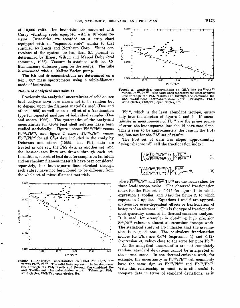
DOE, TATSUMOTO, DEL~VAUX, AND PETERMAN B1.73·

of 10,000 volts. Ion intensities are measured with Carey vibrating reeds equipped with a 1011-ohm re­sistor. Intensities are recorded on a strip chart equipped with an "expanded scale" sjmilar to that supplied by Leeds and Northrup Corp. Shunt cor­rections of the system are less than 0.1 percent as determined by Ernest Wilson and Marcel Dube (oral commun., 1966). Vacuum is attained with an SO­liter mercury diffusion pump on the source. The tube is evacuated with a 100-liter Vacion pump.

The Rb and Sr concentrations are determined on a 6-in., 60° mass spectrometer using a triple·filament mode of ionization.

Nature of analytical uncertainties

Previously t.he analytical uncertainties of solid-source lead analyses have been shown not to be random but to depend upon the filament materials used (Doe and others, 1965) as well as on an effect of a fractionation type for repeated analyses of individual samples (Doe and others, 1966). The systematics of the analytical uncertainties for GS/4 lead shelf solution have been studied statistically. Figure 1 shows Pb206/Pb204 versus Pb206 /Pb208, and figure 2 shows Pb206 /Pb204 versus Pb206/Pb207 for all GS/4 data included in the study by Delevaux and others (1966). The Pbi2 data are treated as one set, the PbS data as another set, and the least-squares lines are drawn through each set. In addition, subsets of lead data for samples on tantalum and on rhenium filament materials have been considered separately, but least-squares lines checked through each subset have not been found to be different from the whole set of mixed-filament materials.

0.4500

~ .0

e:. 0.4475 ~ .0 Q..

............. .... ....

Pb 206 /Pb 204

FIGURE 1.-Analytical uncertainties on GS/4 for Pb:.'OO /Pb 201 versus Pb :.'()() /Pb 209

• The solid lines represent the least-squares line through the Pbl2 results and through the combined R~ nnd Ta-ftlament thermal-emission work. Triangles, Pbl2 ; solid circles, PbS/Ta ; open circles, Re.

1.0500'

16.20 16.25 Pb 206 /Pb 204

\FIGURE 2.-Analytical uncertainties on GS/4 for Pb 208/Pb 20'

versus Pb 208/Pb 207• The solid lines represent the least-squrures

line through the Pbl2 results and through the combined R~ and Ta-filament thermal.emission work. Triangles, Pbl2; solid circles, PbS/Ta ; open circles, Re.

Pb204, which is the least abundant isotope, enters only into the abscissa of figures 1 and 2. If uncer­tainties in measurement of Pb204 are the prime source of error, the least-squares lines should have zero slope. This is seen to be approximately the case in the Pbi2 set, but not for the PbS set of results.

The PbS set of data has slopes approximately fitting what we will call the fractionation index:

[(~ (Pb2os !Pb2o1) )] Pb2o1 __ ~(Pb206jPb204) Xpb204-1/2,

(1)

(2)

where Pb208/Pb204 and Pb207 /Pb204 are the mean values for these lead-isotope ratios. The observed fractionation index for the PbS set is 0.945 for figure 1, to which expression 1 applies, and 0.493 for figure 2, to which expression 2 applies. Equations 1 and 2 are approxi­mations for mass-dependent effects or fractionation of isotopes of an element. . This is the type of fractionation most generally assumed in thermal-emission aD;alyses . It is used, for example,. in obtaining high precision Sr87 /Sr86 values in almost all strontium isotope work . The statistical study of Ph indicates that the assump­tion is a good one. The equivalent fractionation indices for PbJ2 are 0.074 (expression 1) and 0.128 (expre:;sion 2), values close to the error for pure Pb204.

As the analytical uncertainties are not completely random, standard deviations cannot be interpreted in the normal sense. In the thermal-emission work, for example, the uncertainty in Pb206/Pb204 ·will commonly have the same sign as Pb207 /Pb204 and Pb208 /Pb204. With this relationship in mind, it is still useful to compare data in terms of standard deviations, as in

B174 ANALYTICAL TEC~QUES

table 2, to give some idea of just how well the data between two samples can be compared. There is no sample size control involved in the statistics quoted in table 2.

Causes of analytical uncertainties

Several tests have been carried out to determine the causes of the fractionation type of effects remaining even when samples are analyzed on a common-filament material. First the precision obtained by multiple analysis of individual sample loads is established. Next, the possible effects of extended analyses, degree of vacuum, other cations, and rapidity of analysis are examined to establish limits that the mass spectrometer may impose on the precision of the ratio measurements. Finally, the sample-loading effect is established and discussed.

Individual sample loads.-ln order to determine the analytical uncertainties due solely to mass spectrom­etry, three samples were tested. They were loaded, analyzed, and then removed from the mass spectrom­eter. They were then reanalyzed a number of times over a period of a year in 1 of 2 mass spectrometers (table 3). Sample 1 of table 3 was not of normal intensity, and data were usually recorded on a de­creasing ion signal. The other two samples had normal intensity, and data were recorded on growing signals. Data are recorded as ratios of Pb206/Pb204

, Pb206jPb207,

and Pb206/Pb208, and much of the discussion that follows

will involve only these three ratios. The ranges observed in each ratio for samples 1, 2, and 3, as per­centage of each ratio, are given in table 3. When there are no chemical effects present, ratios then can be measured with ranges of 0.3 percent for Pb206/Pb204, and 0.15 percent for Pb206/Pb207, and 0.25 percent for Pb206/Pb208 averaged and rounded to the nearest 0.05 percent. The data for Pb206/Pb207 are probably better than for the other two ratios because the two isotopes are only of one mass unit difference and are of about equal abundance. These factors minimize effects of electronic fluctuations of the instrument as well as any fractionation of lead isotopes that might occur in the mass spectrometer.

Some investigators have suggested thrut one possible uncertainty in the measurement of lead-isotope ratios by solid-source mass spectrometry is lack of reprodu­cible posi·tioning of the sample fi.la.ment on the optic plane. To test this possibility, the filament was bent from its original position in the x-y plane (the plane of the tube) and realined for some runs (table 3). The resulting data on samples 1 and 3 are well within the range of the other data so that sample positioning does not seem to have an effect. There is also no effect re­sulting from analyzing the samples on different mass spectrometers of the same design, such as mass spectro­meters 1 ·and 2 (table 3) .

Extended analyses.-Examples of results of individ­ual analyses over a long period of time are shown in

TABLE 3.-Comparative analyses of single lead-isotope sample loads given by (1) two different mass spectrometers, (2) different positions of filament, and (3) redeterminations at different times throughout one year

Pb-isotope ratios Sample Lab. No. Mass Date

spectrometer 206/204 207/204 208/204

1 _____________________________ 4T282 1 2 3-19-65 18. 162 15. 80 38. 92 1 3-27-65 18. 149 15. 79 38.90 2 5-19-65 2 18. 146 15. 78 38. 94 1 9-13-65 3 18. 172 15.80 38. 90 1 11-26-65 3 18. 195 15.84 39.08 1 3-21-66 3 18. 172 15. 82 39. 02

Ranges in ratio as percentage ---------- ---------- ------------ . 28 . 38 . 46 of mean value. 2 _____________________________ 2T275b 2 3-18-65 17. 090 15. 61 38. 51

1 3-27-65 17. 108 15.62 38. 56 2 5-19-65 17. 095 15. 62 38. 54 1 9- 2-65 3 17. 119 15.65 38. 63 1 11-26-65 3 17. 118 15.65 38. 66 1 3-17-66 3 17. 139 15. 68 38.72

Ranges in ratio as percentage of mean value.

---------- ---------- ------------ . 29 . 44 . 55 3 _____________________________ 2T275a 2 3-18-65 17. 276 15.64 38. 55

1 3-27-65 2 17. 290 15. 63 38. 55 2 5-19-65 17. 299 15. 65 38. 58 1 9- 9-65 3 17. 300 15. 66 38. 61 1 11-26-65 3 17. 302 15. 66 38. 64 1 3-18-66 3 17. 313 15.67 38. 67

Ranges in ratio as percentage of mean value.

---------- ---------- ------------ . 27 . 26 . 31

t Sample 4T282 on mass spectrometer 1 was preceded by three runs spiked with pure Pb200 and Pb20s

2 Filament bent out of the way and then realined. a Second analyst.

206/207 206/208

1. 1493 0. 4667 1. 1495 . 4666 1. 1496 . 4660 1. 1500 ·. 4660 1. 1488 . 4656 1. 1486 . 4657 . 10 . 25

1. 0948 . 4438 1. 0950 . 4437 1. 0942 . 4436 1. 0937 . 4432 1. 0936 . 4427 1. 0931 . 4427 . 17 . 25

1. 1048 . 4482 1. 1059 . 4485 1. 1056 . 4484 1. 1050 . 4480 1. 1047 . 4478 1. 1046 . 4477 . 12 . 18

..

r-

DOE, TATSUMOTO, DELEVAUX, AND PETERMAN Bl75

"' ~ .... 0 > !:

i'l .&l g..

... 0

i!: iii

~ ~

!:

.&l e: i'l .&l

g..~

e:: lS .&l c..

2 .&l

e:: lS .&l g..

0.4550

0.4540

0.4530

1.0700

1.0690

1.0680

16.81

16.80

16.79

16.78

16.77 0

~·-·-·---·--·-~~.~::crt

i /

_,;'$'-----f:-/. T

/ 0.1 percent / '_L

10 20 30 40 50 60 70 80 90 100 10 20 30 40 50 60 70 80 90 200

MINVlES

FIGum~ a.-Extended mass-spectrometer analysis of CIT shelf lead reference sample. Crosses represent m(:'ans for dots in each cluster. 'l"'he intensity of Pb200 decreased 38 percent froon the mu.ximum intensilty observed during the test. Ranges of 0.1 percellJt of each ratio are shown at the right-hand side of the graph for each isotope ratio to give a scale against which to compare observed variaJtJions in each isotope ratio.

figures 3 a,nd 4. No systemic change in ratios with time is observed. The intensity of the Pb206 signal, ex­pressed ns volts, is shown at the top of figures 3 and 4. Figure 3 is an extended analysis of a sample of lead· extrn.cted from J(-feldspar, n.nd ranges in the means of

~ 1.5

~ !:

lS .&l g..

... 0

0.5 ~ iii

~ !:

~ .&l e: 15.300

lS .&l c..

~ 20.10

e: lS .&l c..

./·--- ·--- T ·~r~t

I i

i ....... · REFOCUS MAGNET

1 0.1 percent ,

T -:~ • ·+ +-·----- ~. . ~~ :

MINUTES

l!""rouiw.: 4.-Measurements at different times during >the ex­tended muss-spectrometer analysis of the Tilton 20:1 gravi­metric lead mixture. 'l'he intensity of Pb~00 decreased 20 per­eent from the maximum intensity observed during the test. Ranges of 0.1 percent of each rtrutio are shown at the left­hand s·ide of the graph for each isotope mtio to give a scale ngn·inst which to compare observed variations of each ratio.

the ratios are about 0.1 percent. Figure 4 is an extended analysis of a spectrographically pure lead-isotope mix­ture (often referred to as the Tilton 20 :1 gravimetric mixture) with ranges in the 1neans similar to the K­feldspar sample. Refocusing the magnet during the test had no effect on the analytical results. This lack of a fractionation effect with time is contrary to obser­vations on lighter elements. For one example, Shields and others (1961) noted a 0.2-percent change inAg107

/

Ag109 over a 20-minute span of time. Vacuum.-The possible effect of degrees of vacuum

between 3 and 13 X 10-s mm Hg on resulting data was tested by loosening the flange on the source area of the m·ass spectrometer and then gradually tightening it. The degree of vacuum was monitored at the mass spec­trometer tube. Again possible effects are less than 0.1 percent. Data are usually taken between 6 to 10 X 10-s mm Hg in the tube.

Effect of other catio'f/.8.-Lead-isotope ratios were measured as a function of N a signal, expressed as volts, during runs on two different samples. Effects of other cations on the analytical results are less than 0.1 percent of a ratio. At normal running tempera­tures, sodium and potassium are the only common cations formed. The sodium probably comes from the borosilicate glassware used in the precipitation step and has a measured intensity 10 t<> 100 times the lead signal. Potassium is not abundant in analyses, even though l(CN is used in the chemical purification of lead.

Rapidity of analysis.-Table 4 shows the results of tests with different mass spectrometers and different techniques of ·analyzing samples. On May 13, 1965, two filaments were loaded by operator B within min­utes of precipitating some shelf-lea;d solution. The samples were inserted simultaneously in the two mass spectrometers. Operator A gradually raised the fila­ment tempenature of ·one mass spectrometer, and a lead signal was observed in about 20 minutes. Opera­tor B rapidly raised the filament temperature on the other mass spectrometer, and a lead signal was ob­served in about 1 minute. Data were accumulated starting a:bout 12 minutes after the mass spectrometer was turned on. Operator A then prepared two fila­ments with lead from the same shelf solution a week later in the same manner, and the analyzing procedure was repeated. F•or each individual date, the data are in excellent agreement, indicating no operator effect on the mass spectrometer, but the differences between dates are 2-3 times those expected if no sample load­ing is involved. There appears to be, therefore, some effect in the sample-precipitation and filament-loading steps, as these were the only two steps involved.

B176 ANALYTICAL TECHNIQUES

TABLE 4.-Effect of rapid versus slow rates of analysis on results for CIT shelf lead (Re-4 filament)

Mass Ph-isotope ratios Sample spectrometer Mass Date Speed of run

operator spectrometer

I I 206/204 207/204 208/204

Precipitated and loaded by operator B

1------------------- A 2------------------- B

1 2

5/13/65 Slow __________________________ _ 16.754 16.720

15.66 15.63

36.85 36.76 5/13/65 Fast __________________________ _

Precipitated and loaded by operator A

3 ___________________ A 1 5/20/65 Slow ___________________________ 16.849 15.78 37.25 4 ___________________

B 2 5/20/65 Fast ___________________________

16.838 15.77 37.24

Differences (percent) between dates for average values of each ratio ________________________ 0.64 0.90 1.62

Sample-lolliding effects are further illustrated in table 5, which shows results of "aging" for a sample loaded and analyzed on April 13, 1965, and reanalyzed nearly a month later from the same precipitate lo31ded on another filament.

TABLE 5.-"Aging" effect of lead from Niland, Calif., brine (Ta-1 filament, one precipitate)

[Determinations made by operator B on spectrometer 1]

Sample Date Ph-isotope ratio

206/204 207/204 208/204

! ______________ 4/13/63 19. 288 15.85 39.66 2 ______________ 5/10/63 19. 147 15.69 39. 12

Difference (percent) between dates for each isotope ratio ____________ 0. 75 1. 02 1. 35

Sample-loading e.ffect.-8ample-loading effect could have several causes, and we attempted to isolate them by two experiments. The first experiment was to determine if the amount of lead precipitated in a con­stant volume of NH4N0 3 solution has any effect (fig. 5). In this procedure, 20, 40, and 80 J.£g of Pb were each precipitated in 2 ml of NH1N03 solution, and the total Pb sample with a proportional volume of NH40H solution was loaded on filaments within a few minutes of precipitation. Most analyses of samples are made in the range 20-40 JJ.g of lead. Certainly there is no large effect on the measured ratios, even though different mass spectrometers and operators were used. Thus the precipitation step is not critical, at least on spectrographically pure shelf solutions of lead.

37.1.------------------------.

37.0 - 0 0 • 0

~ .!:J • e:: 36.9 -

11! .!:J p..

36.8 1-

• 36.7 I I I I 16.9

~.!:J e:: 16.8 1--

~ 0 0 .!:J p.. •

16.7 I ' I I 0 20 40 60 80 100

Pb LOAD, IN MICROGRAMS

FIGURE 5.-Lead~isotope ratios measured for CIT shelf lead 1 when the size of the lead load is proportional to the volume of NH4NOa loaded on the filament. Open squares, determined by operator A; solid squares, determined by operator C.

In the second test, the volume of solution loaded on a filament was held roughly constant, but the lead loaded was varied between 20 and 80 ,.,.g (fig. 6). A definite effect is observed with greater lead-isotope ratios

,~·

. .,

DOE, TATSUMOTO, DELEVAUX, AND PETERMAN B177

~ ,t:l

e:. ~ ,t:l ll.

~ ,t:l

e:. ~ ,t:l ll.

37.0.--------------------------.,

36.91-

36.81-

36.7 1-

36.6 1-

36.5 1-

36.41-

I

• •

•

• • •

•

• •

•

•

I I I I 36.3 ._ ___ ..._ ___ .....__ ___ .....~.-___ __._ ___ __,

16.5.-----------------------.,

16.4 1--

16.3 1- I •

I •

• • I •

I I I I 16.2 ._ ___ ..._ ___ ...~...-___ .....~..-___ _._ ___ _.

0 20 40 60 80 100 Pb LOAD, IN MICROGRAMS

kwum~ 6.-Measured lead-isotope ratios for GS/4 shelf lead when the size of the lead load is varied, but the volume of NH4N0s solution londed on the ftl::unent is held approximately constant.

accompanying larger lead loads. There is no overlap of the data for Pb208/Pb204 from 20-~g loads with data frmn 80-~g loads. The difference in the means of the extreme loads is 0.9 percent for Pb208/Pb204

. The data on the smaller lead l?ads is somewhat better than for the larger lead loads-about 0.6 percent range for Pb208/Pb204 of 20-~g loads and 0.8 percent for 80-~g lead loads. This sort of effect could well account for the common observa­tion that values of Pb207/Pb204 are greater in ores than in rocks with similar ratios of Pb206/Pb204. In analyzing ores, one probably loads more lead when it is available, but the volume of solution loaded is usually about con­stant. The theoretical reasons for the sample loading effect are not known.

REFERENCES

Delevau.x, M. H., Pierce, A. P., and Antweiler, J. C., 1966, New isotopic measurements of Colorado ore leads, in Geological Survey Research 1966: U.S. Geol. Survey Prof. Paper 550-C, p. C178-C186.

Doe, B. R., Hedge, C. E., White, D. E., 1966, Preliminary in­vestigation of the source of lead and strontium in deep geothermal brines underlYing the Salton Sea geothermal basin: Econ. Geology, v. 61, p. 462-483.

Doe, B. R., Tilton, G. R., and Hopson, C. A., 1965, Lead isotopes in feldspars from selected granitic r-ocks associated with regional metamorphism: Jour. Geophys. Research, v. 70, p. 1947-1968.

Fleischer, Michael, 1965, Summary of new data on rock samples G-1 and W-1, 1962-1965: Geochim. et COSihoc~im. Acta, v . 29, p. 1263--1284.

Shields, W. R., Garner, E. h, and Dibler, V. H., 1961, Absolute isotopic abundance of terrestrial silver: Jour. Research, Natl. Bur. Standards, v. 66A, p. 1-3.

Tatsumoto, M., 1966, Isotopic c;omposition of lead in volcanic rocks from Hawaii, Iwo Jima and Japan: Jour. Geophys. Research, v. 71, v. 1721-1.,733.

Tilton, G. R., Patterson, C. C., Brown, H., Inghram, M., Haydon, R., Hess, D., and Larsen, E., Jr., 1955, Isotopic composition and distribution of lead, uranium, and thorium in a Pre­cambrian granite: Geol. Soc. An1erica Bull., v. 66, p. 1131-1148.

GEOLOGICAL SURVEY RESEARCH 1967

A METHOD FOR THE ANALYSIS OF FLUID INCLUSIONS

BY OPTICAL EMISSION SPECTROGRAPHY

By JOSEPH HAFFTY and DARRELL M. PINCKNEY, Denver, Colo.

.tibstract.-A spectrographic method is described for the de­termination of calcium, magnesium, and sodium in fluid inclu­sions whereby 200 microliters of solution is evaporated onto a pair of flat-top graphite electrodes. Uni-arc conditions are then used to excite the residue, thereby providing good sensitivity.

A primary fluid inclusion is usually a very small amount of fluid trapped in a oavity of a growing crys­tal. The cavity therefore contains a sample of the fluid fro~ which the crystal has formed (fig. 1). Con­sequently, analysis of fluid inclusions aids in under­standing the chemical environment during crystalliza­tion of minerals and ores.

The recovery ·and preparation of the fluid for anal­ysis follow the procedure described by Roedder and others (1963). The recovered sample of fluid gen­erally has a volume of 10 to 20 milliliters and has been diluted from its original state of concentration by a factor of 2,000 to 7,000. A suitable method for anal­ysis of the fluid must be one that works on small sam­ples and one that is oapahle of determining the kind and amount of many elements that may be present in the sample. The method described here meets these requirements.

The method of optical emission spectrography de­scribed in the present paper is designed to determine calcium, magnesium, and sodium in the spectral region 2400-4800A, where many of the elements present in fluid inclusions are sought. Other elements can be included in the list of elements determined when the present procedure for obtaining the fluid from the inclusion is modified. Potassium is not included in the list of elements determined because a separate exposure is required to measure the 7664.91A line. It is con­sidered more convenient and. practical to analyze for this one element by atomic-absorption spectroscopy.

Previously a "copper spark" procedure for the anal­ysis of calcium, magnesium, and strontium in liquids was reported (Alexander and others, 1954). How­ever, copper concentrations in fluid inclusions are of interest and therefore copper electrodes can not be used. In addition to this, copper electrodes involve a handling problem whereby they have to be machined on a lathe and are not very satisfactory for use with acid solutions. The graphite electrodes come pre­formed and ready for use.

APPARATUS AND OPERA'TING CONDITIONS

Excitation source.-Manufacturer's designation: spark-ignited full-wave uni-arc (see text), with 280-volt power supply. Radio frequency current, amp____________________ 1. 9 The parameters of the initiating circuit are as follows:

Capacitance, pf_ _ _ _ _ _ _ _ _ _ _ _ _ _ _ _ _ _ _ _ _ _ _ _ _ _ _ _ _ _ _ 0. 0025 Inductance, ~'h _______________________________ Residual Primary resistance, dial setting_________________ 5 Secondary resistance, ohm _____________________ Residual Discharge voltage, v _ _ _ _ _ _ _ _ _ _ _ _ _ _ _ _ _ _ _ _ _ _ _ _ _ _ 15, 000 Number of discharges per half cycle___ _ _ _ _ _ _ _ _ _ _ 7 Current, amp, rf______________________________ 5. 5

Spectrograph.-Folded, 3-meter, Rowland circle-mounted grating with 21,000 lines per inch giving a reciprocal linear dispersion of 4A per mm in the first order.

Wavelength region, angstroms _____ ._____ 240G-4800, first order Slit width, microns________________________________ 40 Illumination ___________________ Arc image focused on grating Analytical gap, mm ____________________ - _______ - _- 3 Transmission, percent_ _________ -_-_-_-_-_-_-_-_--- 100 Exposure, seconds_ _ _ _ _ _ _ _ _ _ _ _ _ _ _ _ _ _ _ _ _ _ _ _ _ _ _ _ _ _ _ _ 20 Electrodes ____________________ - __________ ASTM type C-3

ANALYTICAL PROCEDURE

Standards containing the cations calcium, magne­sium, potassium, and sodium are made in a 1-volume­percent hydrochloric acid solution. The concentra­tions of these elements are based on analyses of fluid inclusions reported in the literature (Hall and Fried­man, 1963). The stock solution which was used to pre-

U.S. GEOL. SURVEY PROF. PAPER 575-B, PAGES Bl78-Bl80

B178

HAFFTY AND PINCKNEY B179

•

' , .

...

FIGURE 1.-Fluid inclusions iri fluorite crystal. The cuboid body is a cavity containing liquid and a spherical gas bubble. Other fluid inclusions appear as tiny specks or larger bodies which are out of focus.

pare a series of standard solutions covering the ranges of concentrations indicated in table 1 contained 464 parts per million of sodium, 100 ppm of calcium, 46.4 ppm of magnesium, and 46.4 ppm of potassium. The standards, including potassium, are analogous to the average naturally occurring material described by Hall and Friedman ( 1963). The inclusion of potassium makes possible the use of the same standards for its determination by 3itomic absorption.

To minimize the effect of the wide range of element concentration found in fluid inclusions, it is necessary to incorporate a buffer-internal-standard system in the analysis. Four parts by volume of unknown sample are mixed with o~e part of a buffer-internal-standard solution containing lithium as buffer and molybdenum as internal standard. The lithium in the final mixture is equivalent to 50 ppm and the molybdenum to 0.1 ppm.

Two flat-top graphite electrodes are first water­proofed with two drops each of a petroleum-ether solution of Apiezon "N" grease (5 g/liter) . One hundred microliters of the unknown sample or the standard, both containing the buffer-internal standard, are added to each electrode in 50 J.Ll increments and evaporated by means of a heat lamp. The electrodes are kept under the heat lamp until placed in the arc­spark stand. Each exposure consists of exciting the residue of 200 1-'l of solution on the 2 electrodes.

The type of excitation source used (spark-ignited full-wave uni-arc) is an intermittent d-e arc. The primary power source is a full-wave rectified 280-volt power supply. The primary power source is initiated by a high-voltage condensed spark synchronized to initiate each half cycle. The arc is carried on both halves of the cycle, thereby exciting the residue on the two electrodes.

Spectra are recorded on SA-l plates and calibrated by means of an iron bead arced at 5 amps d-e and exposed for 15 seconds at a transmission of 4.8 percent. The iron bead is formed prior to use by successively arcing portions of iron powder at 5 amps in a large (about X-inch inner diameter) cupped electrode until the bead extends up above the sides of the cup (Haffty, 1960). The iron lines used for calibration were selected from a list of homologous lines (Crosswhite, 1950; Bastron and others, 1960).

The analytical and the internal-standard lines used in constructing the analytical curves are listed in table 1 along with their concentration ranges. The concen­trations read from the analytical curves, an example of which is shown in figure 2, are multiplied by the factor

TABLE I.-Analytical line pairs used in analysis of fluid inclusions

Element

Calcium ___ __ ___ {

Magnesium _____

Sodium _____ __ __ {

10

u::O

s ·

4

3

2

"I 0 ........ 1.0

0.5

0.4

0.3

0.2

Analytical line Internal-standard Concentration (angstroms) line (angstroms) range (ppm)

Ca 4302. 53 Mo 3170. 35 0.20 to 8.0 Ca 4318. 65 Mo 3170. 35 2.0 to 37

Mg 2779. 83 Mo 3170. 35 .05 to 4.0 Na 3302. 32 Mo 3170. 35 .80 to 17 Na 3302. 99 Mo 3170. 35 .80 to 37

CALCIUM, IN PARTS PER MILLION

FIGURE 2.-Analytical curve used for the determination of cal­cium, in fluid inclusions, from the ratio of the intensity (I) of calcium to that of molybdenum, the internal standard.

B180 ANALYTICAL TECHNIQUES

TABLE 2.-Comparison of spectrographic and atomic-absorption analyses of composite leaches of;fluid inclusions [In parts per million]

Magnesium Sodium Calcium

Sample No. Spectrographic Atomic

Spectrographic Atomic

Spectrographic Atomic

absorption absorption absorption Runl Run2 Runl Run2 Runl Run2

23 ___________________ 0. 06 o. 05 0. 062 6. 2 6. 0 5. 9 1.9 1. 8 1.7 30---------------~--- . 17 . 16 . 15 9. 0 8. 9 11 17 18 18 36 ___________________ . 13 . 13 . 098 1. 1 1. 3 1. 0 . 75 .68 .60 29 ___________________

---------- ---------- ---------- ---------- ---------- ---------- 320 360 330

1.25, owing to the addition of the buffer-internal­standard solution. When the concentrations of the elements are high the samples are diluted to bring them in range of the analytical curves. Good compar­ative data were obtained for calcium on sample 29 (table 2), which was diluted 1:99 for the spectro­graphic result and 1 :199 for the atomic-absorption result.

A measure of the accuracy is obtained by comparing the spectrographic results with those obtained by ·atom­ic-absorption spectroscopy (table 2). In order to have sufficient sample for the accuracy tests made, composite samples (table 2) were submitted. These samples rep­resent composites of water and acid leaches of fluid inclusions and are not intended for any geologic inter­pretation.

REFERENCES

Alexander, G. V., Nusbaum, R. E., and MacDonald, N. S., 1954, Strontium and calcium in municipal water supplies: Am. Water Works Assoc. Jour., v. 46, p. 643-654.

Bastron, Harry, Barnett, P. R., and Murata, K. J., 1960, Method for the quantitamve spectrochemical analysis of rocks, min­erals, ores, and other materials by a powder d-e arc tech­nique: U.S. Geol. Survey Bull. 1084-G, p. 165-182.

Crosswhite, H. M., 1950, Photoelectric intensity merumrements in the iron arc: Spectrochim. Acta, v. 4, p. 122-151.

Ha:trty, Joseph, 1960, Residue method for common minor ele­menits: U.S. Geol. Survey Water-Supply Paper 154D-A.

Hall, W. E., and Friedman, Irving, 1963, Composition of fluid inclusions, Cave-in-Rock fluorite di strict, Illinois, and Upper Mississippi Valley zinc-lead district: Econ. Geology, v. 58, p. 886-911.

Roedder, Edwin, Ingram, Blanehe, and Hall, W. E., 1963, Studies of fluid inclusions III-extraction and quantitative analysis of inclusions in the milligram range: Econ. Geology, v. 58, p. 353-374.

GEOLOGICAL SURVEY RES~ARCH 1967

DATA ON THE ROCK GSP-1 (GRANODIORITE)

AND THE ISOTOPE-DILUTION METHOD OF ANALYSIS FOR Rb AND Sr

By ZELLE. PETERMAN, BRUCE R. DOE, and ARDITH BARTEL, Denver, Colo.

A.b8tract.-Ooncentrations of selected elements in the U.S. Geological Survey standard granodiorite, GSP-1, as determined by isotope dilution are 268 ppm of Rb, 240 ppm of Sr, 58.7 ppm of 2.4 ppm of U, lUl.d 106 ppm of Th. Duplicate analyses of Rb, Sr, nnd Pb n.gree to witMn 1 percent. Replicate analyses of U and Th show larger variations. The range in U values is ±20 percent of the menu allld in Th value, ±8 percent of the mean. The iootop'ic compositionS' of Pb and Sr are given, and the analy­tical techniques for the determination of Rb and Sr are discussed. The Sr 87 /Sr 80 ratio after nonnalization is 0.7687±0.0011. Tbe isotopic composition of lead is given by the followill!g ratios: Pb 200/Pb 20

', 18.077; Pb !!07 /Pb 20\ 15.67; and Pb 208 /Pb 204

, 47.33.

This paper is one in a series reporting isotope-dilu­tion analyses of selected elements in a group of stand­ard rock samples prepared by the U.S. Geological Survey. Doe and others (1967) have dealt with the standard granite G-2 and have discussed the deter­mination of lead by isotope dilution and the isotopic analysis of lead. In the present report, isotopic data for the standard granodiodite GSP -1 (split 1, position 23) are presented, and the analytical techniques used in the isotope-dilution ·analyses for Rb and Sr and in the isotopic analyses of Sr are discussed.

The standard rock sample GSP-1 is a granodiorite collected from the Precambrian Silver Plume Granite near Georgetown, Colo., in the Colorado Front Range.

RESULTS

Concentrations of the selected elements Rb, Sr, Ph, Th, and U tLre given in table 1. Of these, U shows the greatest spread in the replica .. te analyses, for which the total range can be expressed as ±20 percent of the mean v·alue. l"'he range in the Th concentrations is±8 percent of the mean. The duplicrute analyses for Rb, Sr, and Pb agree to within 1 percent. The large ranges in U and Th a .. nalyses are clearly outside of normal analytical uncertainty as indicatd by replicate analyses of volcanic

rial which results in difficulty in obtaining a representa­tive aliquot of a material in which the minor elements may be strongly concentrated in accessory minerals. The U and Th contents of the two aliquots, which were split with a microsplitter ( ta;ble 1) , are in closer agreement than those that were poured from the sample bottle. The means of these samples are used as the preferred values.

Isotopic anallyses of Pb and Sr are given in table 2. The precision of Pb isotopic ana1lyses has been discussed by Doe and others (1967) (p. B173, this chapter). Because of the variations in Pb isotopic ratios, that are due in part to the filament material used (Doe and others, 1965), both the observed rUJtios (on Re, lot 6) and the converted values (Ta, lot 1) are shown in table 2. The conversion is accomplished by adjusting the observed values by amounts determined through repli­cate analyses of standard samples on the v.arious fila­ment materials. A detaHed discussion of the Sr iso­topic analyses is given in following sections of this paper.

TABLE I.-Concentrations of selected elements in the standard granodiorite GSP-1

Sample .... ~ Dissolution method ~

= <

Concentration (ppm) Type of sample aliquot Rb Sr Pb U Th

---__ , _______ , _____ ,_- --------l _______ _ 2 _______ _ 3 __ ------4 __ ------5 _______ _ 6 _______ _ 7 _______ _

(1) HF-H2S04 _____ Spatula __ 269241 ____ --- __ _ (1) _____ do __________ do _____ 267 239 _________ _ (2) HF-HC104 ____ Poured _____________ 2. 2109 (3) _____ do __________ do _______________ 3. 3 117 (3) _____ do _______ Split _______________ 2. 2105 ( 4) _____ do _______ Poured _________ 58. 7 3. 2120 ( 4) Borax fusion__ Split ___________ 58. 6 2. 5 108

Mean values __________________________ -12681240158. 712. 71112 Preferred values ________________________ 26824058.72.4106

1 Z. E. Peterman and W. T. Henderson. glasses (B. R. Doe, unpub. data). These may be the 2 R. K. Price. • a Ardith Bartel and M. H. Delavaux. result of nuneral inhomogeneities in the powdered mate- • B. R. Doe, Ardith Bartel, and M. ii. Delavaux.

U.S. GEOL. SURVEY PROF. PAPER 575-B, PAGES Bl81-Bl86

B181

TABLE 2.-Isotopic composition of Pb and Sr in the standard granodiorite GSP-1

Sample Analyst Filaments Dissolution method Sr-isotope ratios Ph-isotope ratios

SrS6fSrSs SrS7/SrS6 (Sr87f8r86) 0 1 1 Pb206/Pb204 Pb207/Pb204 Pb20S/Pb204 Pb206/Pb207 Pb206/Pb20S ·----1----1 I I I I I I I 1---~-

1 ____________ _ 2 ____________ _ 3 ____________ _ 4 ____________ _ 5 ____________ _ 6 ____________ _

(2) (2) (3) (3) (4) (4)

Re __________________ HF-H2SO•------ 0.11974 0. 7676 0. 7687 Re _______________________ do_________ .11973 . 7675 . 7686 Re, lot 6 _____________ HF-HC104------ ---------- ___________________ _ Ta, lot-1 conversion ________ do ___________________ ---------- _________ _

·Re, lot 6 __________________ do _________ :.. ____________________________ _ Ta, lot-1 conversion ________ do _________ ---------- ___________________ _

3B. R. Doe.

18. 169 18. 071 18. 183 18. 084

1 SrB7/SrB6 normalized to a SrB6/SrBB ratio of 0.1194. 2 z. E. Peterman and W. T. Henderson. • B. R. Doe and M. H. Delavaux.

,}-.

15.79 15. 66 15.80 15.67

47. 76 47. 24 47.93 47.41

1. 1506 1. 1537 1. 1511 1. 1543

0.3804 . 3825 . 3794 . 3814

t;d ~

~

~ 1-t a ~ 8 l"'.l a

~ £) ~ l"'.l Ul

PETERMAN, DOE, AND BARTEL Bl83

Some unusu·al ratios of elements in granodiorite GSP-x are of speci1al geochemical interest. The ratio p. (U288 /Pb204 ) is 2.95 and is the lowest value observed for intermediate to silicic igneous rocks. The ThjU ratio is 44.3 and is abnormally high, because most crustal rocks have Th/U ratios less than 10 and more commonly between 2 and 6.

The unusually high Th/Pb ratio and a Rb/Sr ratio of 1.12 allow caloulaJtion of the Th/Pb and Rb/Sr total­rock ages. Assuming an initial SrB7 /SrB6 ratio of 0.703 the Rb/Sr age is 1.36'±0.05 billion years (using the 47-b.y. half life for Rb87

). This is in agreement with a total-rock isochron age of 1.37 b.y. obtained on the Longs Peak Granite of Fuller (1924), which is typical of Silver Plume Granite (Z. E. Peterman, C. E. Hedge, and W. A. Braddock, unpub. data).

Similarly, the Thz82 /P'b2°8 age can be calculated by .assuming an initial Pb2°8 /Pb204 ratio. If an iniltial ratio such as that observed for feldspar leads from the St. J{evin Granite of the Sawatch Range is assumed (Doe, 1967), the calculated age is 1.55 b.y. If a more precise Th/Pb age is to be obtained, it would be necessary to determine the initiaJl Pb208 /Pb204 ratio; however, within the lirillts of uncertainty the Th/Pb and Rb/Sr ages are in agreement.

ANALYTICAL METHODS FOR Rb AND Sr

Most of our work dealing with Rb and Sr is an ap­plication of the Rb87 - Sr87 decay scheme to the meas­urement of geologic time and to Sr isotopic tracer studies. The following discussion is therefore limited to the methods used in determining Rb and Sr in sili­c.nte samples.

An extremely important part of the procedure for dating rocks and minerals is sampling and sample preparation. For the analyses of total-rock samples, 1 kilogram or more of sample is colledted, depending on grain size and uniformity of the rock. The samples are crushed to -40 mesh and carefully split to produce a, minimum size sample of 15 grams. These splits are pulverized to rubout -200 mesh and thoroughly mixed. The final splits for analyses are made ei.ther with a microsplitter or hy carefully mixing the sample by roliJ­ing it on paper and taking random portions with a spatula.

'Reagents 'l'he following reagents are used in the chemical preparation

of silicate samples for Rb and Sr analyses: Water: triple distilled, using a Barnstead still coupled with a

400 ml/hr Engelhard double-stage quartz still. Hydrochloric acid : 6.2N HCl prepared by bubbling commercial

HCl gas through triple-distilled water in a polyethylene bottle. 2.5N HCl prepared by diluting 6.2N HCl with triple-distilled water.

Hydrofluoric acid: 48 to 51 percent, commercial analytical grade. Sulfuric acid : concentrated, commercial analytical grade.

Spikes

The Rb and Sr spikes were obtained from the Oak Ridge National Laboratory and are enriched in Rb 87

and Sr86, respectively. These were dissolved in triple­

distilled water to obtain the primary spike solutions. Aliquots of the primary solutions are diluted volumetri­cally by a factor . of 50 to obtain the working spike solutions. Concentrations, in micrograms per milli­liter in the working spikes at the time the present analyses were made are given below:

Rbss ________ -=--- 0. 0364 Srs6 _____________ 8. 327 RbB7 ____________ 4. 368 SrB7 ______________ . 0577

Srss ______________ . 1505

Concentrations of the spike solutions are checked at least every 6 months against standard solutions of normal Rb and Sr. These standards are prepared from 99.95 percent pure Sr(N03)2 obtained from John­son, Mathey and Co., Ltd., and from 99.8 percent pure Rb2S04 obtained from United Mineral and Chemical .Corp. Standard solutions of about 2,000 J.tg/ml of Rb and Sr are prepared and calibrated gravimetrically. These are also checked at least every 6 months.

Blanks

During the last year (1965) a number of determina­tions indicated that the blanks have been about 0.02 J.tg Rb and 0.04 J.tg Sr for an analysis. Because these are well below the precision of the method no correc­tions are made.

Sample dissolution

Depending on the Rb and Sr concentrations in the rock or mineral as estimated from preliminary X-ray fluorescence analyses, between 0.3 and 0.6 gram of sam­ple is weighed in a 40-ml Pt dish. Accurately meas­ured volumes (by calibrated pipets) of Rb and Sr spike solutions are added to the sample along with 0.5-ml concentrated sulfuric acid. The spike solutions are evaporated down to the sulfuric acid on a hotplate at 250°-275°C. About 25 ml of hydrofluoric acid is added, and the sample is digested at 250°-275°0 on a hotplate. Hydrofluoric acid is added again as needed. When the sample has been completely digested it is taken to dryness and the heat is raised to 350°-375°0 until the sulfuric acid is fumed off. This rids the sample of all hydrofluoric acid and converts the re­maining cations to sui fates. The dish is removed from the hotplate, 6 ml of 2.5N HOI is •added, and the resi­due is allowed to leach for about an hour. About half the liquid is centrifuged, transferred to a 5-ml beaker, and taken to dryness. This aliquot. is used without further purification for the Rb analysis.

B184 ANALYTICAL TECHNIQUES

The remaining solution is also centrifuged and passed through an ion-exchange column containing Dowex 50 WX-8 (200--100 mesh) resin to obtain a pur­ified Sr sample. When the proper amount of 2.5N HCl eluant has passed through the column the last 30 ml are collected in a Vycor beaker and taken down to 2 or 3 ml on a hot plate. This is transferred to a 5-ml beaker and taken to dryness. The Sr sample is now ready for analysis.

Unspiked samples for Sr isotopic analyses are pre­pared using the same procedure as outlined above except that the Rb and Sr spiking are omitted.

Sample loading The Rb sample is leached with a small amount of

triple-distilled water. About 1 to 3 drops of the super­natant liquid is loaded onto the Re sample filaments and taken to dryness at 1.5 amperes.

Approximately 5 drops of 2.5N HCl is added to the Sr sample (spiked or unspiked). About half of this is loaded onto theRe sa,.mple filaments and taken to dry­ness at 1.8 amps. Upon dryness, the filaments are heated to a very slight dull-red glow for 2 minutes (2.0 to 2.2 ·amps).

Mass spectrom·eter Nearly all the analyses for Rb and Sr concentration

are determined on a 6-inch, 60° mass spectrometer of the Nier type as modified by W. R. Shields, National Bureau of Standards. A triple-filament mode of ion­ization is utilized. The source, collector, and electron­ics are similar to those of the 12-inch spectrometer described previously by Doe and others (1967) (p. B172, this chapter). Rb and Sr are voltlltilized from two Re sample filaments and ionized by a Re center filament. The ions are accelerated in a potential drop of 5,000 volts.

. Isotopic analyses

Because of the long half life of Rb 87, which is 47'X 109

years according to Flynn and Gle11denin (1959) or 50 X 109 years according to Aldrich and others (1956), it is necessary to determine Rb and Sr concentrations, and Sr isotopic composition to the highest possible degree of precision in order· to reduce to a minimum the analytical uncertain ties of the measured ages.

In the concentration work, the greater part of the analytical uncertainty lies in the chemical preparation of the the samples (sample splitting, weighing, spiking, spike calibrations, and so forth), and not in the isotopic analyses.

Rb analyses.-N atural Rb consists of two isotopes, with masses of 85 and 87. The isotopic composition most commonly assumed is that determined by Nier

(1950), who reported a Rb85/Rb87 ratio of 2.591. More recently Shields a~d others (1963) report a mean Rb85/Rb87 ratio of 2.5995 ± 0.0015 (95-percent confi­dence level) for 27 natural silicate samples. A highly significant contribution of their work is that they found no variations in the isotopic composition of Rb outside of experimental error, and therefore it can be safely assumed that the Rb85/Rb87 ratio is constant in nature. Because of this invariant ratio we do not routinely analyze unspiked Rb samples. However, on our mass spectrometers we do obtain a Rb85/Rb87 ratio for normal Rb identical with that reported by Shields and others (1963). In order to be consistent with other labora­tories and the Rb87 half life determined by Flynn and Glend.enin (1959) our observed Rb 85/Rb87 ratios are normalized to the 2.591 value obtained by Nier (1950).

Sr analyses.-N atural Sr consists of 4 stable isotopes of masses 84, 86, 87, and 88 of which all but Sr87 are assumed to be constant in nature. The abundance of Sr87 has changed with time because of the radioactive decay of Rb87

, which is the basis for the Rb-Sr method of age determination. The commonly accepted values for isotopic composition for nonradiogenic Sr are those determined by Nier (1938), which are Sr84/Sr88 =0.0068 and Sr86/Sr88 =0.1194.

For many samples of the type presently being dated (those with a small enrichment of radiogenic Sr87)

it is necessary to determine the Sr concentrations and Sr isotopic compositions on separate splits. For samples which are considerably enriched in radiogenic Sr87 as a result of a large Rb/Sr ratio and (or) an old age, it is often sufficient to calculate the amount of radiogenic Sr87 from the spike Sr · analysis.

One of the major problems that arises during the isotopic analyses is the fractionation of Sr during the analysis. Fractionation is considerably reduced by using the triple-filament mode of ionization (see Hedge and Walthall, 1963, fig. 1, p. 1214). Other parameters which may be controlled during the anal­yses to reduce fractionation are discussed by Shields and others (1963, p. 2331) with regard to Rb, but they are also applicable to Sr. In order to correct for fractionation effects it is common practice to nor­malize the observed Sr86/Sr88 values to a value of 0.1194, and to adjust the observed Sr87 /Sr86 values half this amount. The normalization procedure assumes .that there are no natural variations in the nonradiogenic Sr isotopes.

The precision of the Sr isotopic measurements is determined by replicate analyses of a standard Sr solution containing 500 p.g of Sr per milliliter (stron.:. tium nitrate, United Mineral and Chemical Corp~,

lot :i3 857), which will be referred to as the USGS

,,

PETERMAN, DOE, AND BARTEL B185

standard Sr. Precision data for the· standard Sr are shown in table 3. In November 1965, an improved technique for analyzing Sr was developed which in­volves sample loading and operation of the filaments at considerably lower temperatures than had previ­ously been done. In the following discussion the new method will be referred to as the "low-temperature method" in contrast to the previously used "high­temperature method." The operating conditions for the filaments (Re ribbon, 1 X30 mils, 0.5 inch in length) are as follows: (1) The center filament is turned to 4.8 amps (approximately 1,600°0) to burn off any Rb present, and the side filaments to· 0.10 amp. Nor­mally 1 to 3 minutes under these conditions reduces the Rb signal sufficiently. (2) The center filament is turned down to 3.8 amps (approximately 1,450°0), and. the Sr signal is increased by turning up the side filaments by increments of about 0.10 amp until a suitable signal is obtained (normally 150 to 300 milli­volts signal for Sr86 with a 2.5 X 1011 ohm resistor in the preamplifier circuit of the Carey vibrating-reed electrometer). Generally, a growing or stable signal is obtained 10 to 20 minutes after the run is started.

TABLE 3.-Precision of Sr isotopic measurements for USGS standard Sr, and for routine rock analyses

SrSGfSrss SrS7fSrse

USGS STANDARD Sr High-temperature method t

~ean________ 0.1200 Range.______ .1196-.1206 u____________ .00035 u (percent)___ . 290

0.7087 .7074-.7097

.00085

.120

Low-temperature method 2

~ean________ 0.1198 Range_______ .1197-.1200 u____________ .00010 u (percent)___ . 083

0.7091 .7085-.7099

.00048

.068

0.7106 . noo-. 7115

.00055

.077

0. 7104 . 710Q-. 7108

.00037

.052

ROUTINE ROCK ANALYSES (IGNEOUS, METAMORPHIC, AND SEDIMENTARY ROCKS) High-temperature method a

~ean________ 0.1200 Range _______ .1194-.1207 u____________ .00033 u (percent)___ . 275

Low-temperature method •

~ean________ 0.1198 Range_______ .1193-.1203 u____________ .00019 u (percent)___ .150

' llnnnlyscs, Mnr. 1965 to Sept. 1965. 2 6 nnnlyscs, Nov. 1965 to Apr. 1966. 3 71 nnnlyscs, Mnr. 1965 to Oct. 1965. • 73 nnnlyscs, Nov. 1965 to Mar. 1966.

A comparison of data obtained on the standard Sr by the low- and high-temperature methods is given in table 3. The improvement in precision for the Sr86 /Sr8 data with the low-temperature method is significant and indi­cates a decrease in fractionation effects. At -the 95-percent confidence level, using Student's t factor for a limited statistical sample, the precision of the Sr6 /SrB8

ratio for a single analysis has been reduced from -+-0.65 percent to -+-0.21 percent. This decrease of fractiona­tion is also shown by comparing the Sr7 /Sr6 data. For the high-temperature method the precision in Sr87 /Sr86 ratios is improved by a factor of 1.6 by the normalization procedure, whereas the Sr7/Sr6 ratios by the low-temperature method are little improved by normalization (table 3) .

Perhaps more applicable to routine analyses of rocks and mine~als are the data shown in table 3 for '71 sili­cate samples determined by the high-temperature method and 73 silicate samples determined by the low­temperature method. The analytical precision of the data is increased by nearly a factor of 2, using the low­temperature method. At the present time it appears that the precision in the Sr86/Sr88 ratios using the low­temperature method is -+-0.30 percent at the 95-percent confidence level.

These data also indicate more precisely than previous results that there is no significant fractionation of Sr in nature. From the 73 analyses by the low-temperature method it can be stated that at the 95-percent confidence level the isotopic fractionation of Sr in natural environ­ments is less than -+-0.30 percent of the Sr86/Sr8 ratio.

For intralaboratory comparison of Sr isotopic data, the standard Sr is analyzed on the various mass spec-. trometers. For comparison with data obtained by other laboratories it is sufficient to report here that on the USGS 6-inch spectrometer, on which the present data were obtained, we have determined Sr7/Sr6 values of 0.7085 on the MIT (Massachusetts Institute of Tech­nology) shelf Sr and 0;7093 for modern sea water.

REFERENCES

Aldrich, L. T., Wetherill, G. W., Tilton, G. R., and Davis, G. L., 1956, Half-life of Rb87

: Phys. Rev., v. 103, p. 1045-1047. Doe, B. R., 1967, The bearing of lead irotopes on the source of

granitic magma: Jour. Petrology, v. 8, p. 1-33. Doe, B. R., Tilton, G. R., Hopson, C. A., 1965, Lead isotopes in

feldspars· from selooted granitic rocks 8Jssociated with re­gional metamorphism: Jour. Geophys. Research, v. 70, p. 1947-1968.

Doe, B. R., Tatsumoto, M., Delevaux, M., and Peterman, z: E., 1967, Isotope-dilution determination of five elements in G-2 (granite), with a discussion of the analysis of lead, in Geological Survey Research 1967: U.S. Geol. Survey Prof. Paper 575-B, p. B170-B177.

B186 ANALYTICAL TEC~QUES

Flynn, K. F., and Glendenin, L. E., 1959, Half-life and beta spec­trum of Rb87

: Phys. Rev., v. 116, p. 744-748. Fuller, M. B., 1924, General features of pre-Cambrian structure

along the Big Thompson River in Colorado: Jour. Geology, v.32,no.1,p.49-63.

Hedge, C. E., and Walthall, F. G., 1963, Radiogenic strontium-87 as an i.ndex of geological processes: Science, v. 140, no. 3572, p, 1214-1217.

Nier, A. 0., 1938, Isotopic constitution of Sr, Bi, Tl and Hg: Phys. Rev., v. 54, p. 275-278.

--- 1950, A redetermination of 'the relative abundances of the isotopes of neon, krypton, rubidium, xenon, and mer­cury: Phys. Rev., v. 79, p. 450-454.

Shields, W. R., Garner, E. L., Hedge, C. E., and Goldich, S. S., 1963, Survey of Rb85/Rb87 ratios in minerals: Jour. Geophys. Research, v. 68, no. 8, p. 2331-2334.

GEOLOGICAL SURVEY RESEARCH 1967

RAPID ANALYSIS OF ROCKS AND MINERALS

BY A SINGLE-SOLUTION METHOD

By LEONARD SHAPIRO, Washington, D.C.

A.bstraot.-Previously reported procedures for the rapid anal­ysis of rocks by spectrophotometric methods now have been supplemented by atomic-absorption spectrophotometric methods for determination of CaO, MgO, Na20, K20, and MnO. A single solution prepared after fusion of the sample with lithium metaborate replaces the two solutions previoUSily used in the rapid-analysis method. As a result of these modifications the 'time required for the complete analysis of a rock has been halved.

Methods described for the rapid analysis of rocks by spectrophotometric methods (Shapiro and Brannock, 1962} have been supplemented now by atomic-absorp­tion spectrophotometric methods for the analysis of CaO, MgO, Na20, K20, and MnO. Atomic-absorption methods have been described by a number of authors (for example, Trent and Slavin, 1964; Billings and Adams, 1964), and the accuracy of such methods has been discussed by Billings ( 1965) .The use of atomic­absorption methods has made possible the substitution of a single solution for the two solutions formerly used in determining the major rock-forming elements. As a consequence, gains in accuracy (especially for MgO) and speed have resulted. For e.xample, with the meth­ods described by Shapiro and Brannock (1962) ·a third of bhe time ~equired for an analysis is consumed in pre­paring the solutions. Now the time required for solu­tion preparation is reduced by 90 percent because of the single-solution procedure described in this paper.

The single-solution method depends on initial fusion of the sample with lithium metaborate. This method originated with Ingrunells (1964), who later suggested its use with atomic-absorption spectrophotometry ( Suhr and Ingamells, 1966) and described spectropho­tometric procedures (Ingamells, 1966} as applied to the

concentration cannot exceed approximately 150 parts per million; otherwise the Si02 will start to polymerize

. and precipitate. On -the other hand, if the solution is too dilute, low levels of the other constituents cannot be determined accurately by the methods described by Shapiro and Brannock ( 1962). A solution, prepared from a rock powder, that is sufficiently dilute for sta:. bility of Si02 is sufficiently concentrated for determin­ing the other constituents, if atomic absorption spec­trophotometry is used.

The solution concentration fmmd to be best is 100 milligrams of sample per liter. This provides a solution that without further dilution allows Si02, Al2Qa, Fe20a, Ti02, and P20 5 to be determined by simp~e spectro­photometric procedures, and CaO, MgO, Na20, K20, and MnO to be determined by atomic-absorption spec­trophotometry. The spectrophotometric procedure for P20s is based on a molybdenum-blue color which is about 100 times more sensitive than the molybdivana­date previously used for silicates, but the other spectro­photometric procedures remain virtually unchanged from those described by Shapiro and Brannock (1962}. With carbonate and phosphate rocks the unusually high content of CaO and P 20s may be determined with some­what better accuracy by simple rapid-analysis ~ethods described for this purpose by Shapiro and Brannock (1962). Ferrous iron, H 20, and C02 must, of course, still be determined on separate portions of sample as also described for the rapid-analysis methods. The equipment for the general scheme of analysis from a single solution is illustrated in figure 1.

PREPARATION OF SAMPLE

rapid analysis of silicates. Weigh 0.10000 ± 0.0001 gram of the sample powder In preparing a single solution suitable for determin- (previously ground to 100 mesh or finer) and transfer

ing Si02, Al:JOa, CaO, MgO, N ~0, K20, F~Oa, MnO, to- a new ~aphite crucible. Place approximately 0.6 g Ti02, and P 205, concentration is a vital factor that must of lithium meta borate on top of the sample. In be considered. If the solution is to be stable, the Si02 addition to the rock samples prepare a blank and 1 or

U.S. GEOL. SURVEY PROF. PAPER 575-B, PAGES Bl87-Bl91

B187 241-834 0-67-18

B188 ANALYTICAL TEC~QUES

2 standards of known silica, alumina, titania, and iron oxide content within the ranges 5Q-75 percent Si02, 12-20 percent Ab03, 1-2 percent Ti02 and 1Q-15 percent Fe203• The granite, G-1, and diabase, W-1, are used as standards in the writer's laboratory. Place the crucibles onto a silica tray and insert into a muffle furnace at 1,000° C after preheating in front of the open furnace for several minutes. Fuse for 1 hour. Remove the resulting fused beads from the furnace and cool to room temperature.

To a series of 1~liter plastic beakers add 1 liter of water. Place the beakers on magnetic stirrers, add Teflon-coated stirring bars, and stir rapidly. Transfer the cooled beads from the crucibles to the beakers. They will come out of the crucible without difficulty if new crucibles are used. Add 15 milliliters of con­centrated HOI. The time required for complete solu­tion of the beads will range from 1 72 to 3 hours, depending on the stirring rate, the shape of the vessel, and other factors. When the pellets have completely dissolved, the solutions are ready to be used.

SP·ECTROPHOTOMETR·IC DETERMINATION

The spectrophotometric determinations, except the one for P205, follow closely the procedures described by Shapiro and Brannock (1962), except for minor changes noted below.

The procedure for the analysis of Si02 is based on the development of a molybdenum-blue color. A pipet to deliver about 4.5 ml is used to take aliquots from the sample solutions; the pipet is best in the form of a stopcock device. Reagents to develop the color are best added by a pipetting machine, but an alterna­tive procedure also can be used. The blank, standards, and sample solutions a~e run at the same time. (See Shapiro and Brannock, 1962, p. A5-A17, A20, and A24 for details of above changes.)

Al203 is determined · from measurements of the absorbance of the color of a calcium aluminum alizarin red-S complex. A pipet to deliver 7-8 ml is used, and either the procedure for machine pipetting or an alterna­tive procedure is followed (Shapiro and Brannock, 1962, p. A20 and A25-A27).

The procedure for analysis of Ti02 utilizes the yellow color produced with Tiron (disodium-1,2-dihydroxy­benzene-3,5-disulfonate). This procedure is the one

described by Shapiro and Brannock (1962, p. A29), except that 50 ml of the sample solution is used in step 1; step 2 is deleted; and in step 4, 20 ml of the buffer is added. The W-1 used as the titanium standard contains 1.1 percent Ti02.

:fe20s (total Fe as Fe203)

Iron is determined from the orange color produced with orthophenanthroline. The procedure is that described by Shapiro and Brannock (1962, p. A28) except that 50 ml of the sample solution is transferred to 10Q-150-ml beakers instead of volumetric flasks, and in step 3, 10 ml of orthophenanthroline is added. No dilution is required after the addition of citrate. The W-1 may be used as the standard and contains 11.0 percent Fe203• Alternatively, iron may be deter­mined by atomic absorption spectrophotometry.

For concentrations of P205 up to 1.0 percent, .a molybdenum-blue method as described below is used. Above 1.0 percent P205 content, the method described by Shapiro a~d Brannock (1962) for phosphate rocks should be used.

Preparation of reagents

Ammonium molybdate solution.-Dissolve 12.5 g of (NH4)sMo70244H·20 in 340 ml of H20; then add 160m] of 1+1 H~04.

Stannous chloride solution.-Orush a few crystals of Sn012·2H20 in a mortar and weigh out approximately 150 mg. Transfer to a small beaker and dissolve in 25 ml of concentrated HOI. Add 25 ml of water. This solution should be prepared at the time it is to be used.

Standard P20 5 solution.-Vsing National Bureau of Standards· standard sample 56b (phosphate rock), prepare a sample solution as with any other sample after a fusion with LiB02. This provides a 31.7 percent P20 5 standard. Transfer 31.5 ml of this solution to a 1-liter volumetric flask and add 10 ml of cone. HOI and about 500 ml of water. Then add and dissolve approximately 0.6 g of LiB02 f,l,nd make to volume. This is the !-percent P20 5 working solution.

Procedure

1. Transfer 50-ml portions of the blank, the 1 percent standard, and the sample solutions to a series of 150-ml beakers, using a ·graduate.

2. Add 2 ml of the ammonium molybdate solution to the first 10 beakers, then add 1 ml of the stannous chloride solution.

3. Four to five minutes after adding the stannous chloride to the first solution, proceed to measure:

SHAPIRO B189

Si02-Molybdenum blue AI20 3 -Aiizarin red-S Ti02-Tiron ~ss=~~m-'*.w&""-~ Spectrophotometer Fe20 3 -Orthophenanthroline P2 0 5 -Molybdenum blue

--~ '

1.5-percent HCI

;~ [J

./ ~~ ~ ~

QCJO

CaO MgO

Muffle furnace

Magnetic stirrer Na20 ~Plus LaCI3 ====~=sm:==m

K20 MnO

Atomic-absorption spectrophotometer

FIGURE !.-Schematic diagram of the equipment used in the •analysis of rocks from a single solution.

on the spectrophotometer, the percent trans­Iuission at 640 m~, using the blank as reference. The blue color developed reaches a peak in 4 minutes and is stable for the next 10 minutes, after which it begins to decrease. Ten solutions can easily be measured in this time span.'

4. Repeat steps 2 and 3 with the remainder of the solu­tions, 10 at a time.

Calculations

1. Convert the reading for percent transmission to absorbance.

2. Compute the factor:

F t 1.00 ac or Absorbance of standard

3. FactorXabsorbance of sample=percentage of P20 5

in sample.

P20s in phosphate rocks

In the analysis of phosphatic rocks, resufting in solutions with concentrations of P20 5 over LO percent, the method described by Shapiro and Brannock (1962, p. A32) is used. The standard solution is the one described for the silicate level P20 5, that is, the solu­tion of NBS sample 56b which is equivalent to 31.7

percent P20 5• For the development of the vanado­molybdate color the· procedure described by Shapiro and Brannock (1962, p. A32) is modified slightly. Steps 1 and 2 are omitted, as the sample solutions are sufficiently dilute. In step 3, 50 ml of sample solution is used instead of the indicated 15 ml. In the 4th step, 15, 25, and 50 ml of the standard solution are used. Otherwise, the procedure is unchanged. This procedure can lead to results within 0.1 percent P20 5,

which is adequate accuracy for percentages above 1 percent but not for those below this level.

CaO in carbonate and phosphate rocks

CaO may be readily determined ~ith 1-2 percent relative accuracy by atomic absorption. This is ade­quate in most cases for the levels found in silicates but not for carbonates and phosphates where CaO can often be 40-50 perc~nt of the rock. Accuracies to within 0.5 percent of the amount of CaO + MgO pres­ent can readily be obtained by using visual titration (Shapiro and Brannock, 1962, p. A38-A40). After the determination of MgO by atomic absorption, the CaO + MgO value can .be used to calculate the CaO value.~ As MgO is generally relatively a minor consti­tuent, the calculated CaO retains the· accuracy inherent in the precise visual titration.

B190 ANALYTICAL TEC~QUES

ATOMIC-ABSOR·PTION SPECTRO'PHOTOMETRIC PROCEDURES

The instrument used in the writer's laboratory for atomic-·absorption spectrophotometric determinations is the Perkin-Elmar Model 303 with a digital readout attachment, but other instruments can be used with comparable results. The fuel used is acetylene-air. The directions provided with any of the instruments are detailed and need not be discussed here, hut a brief description of our technique, which differs slight-, ly from manuf·acturer's suggestion will be given.

Standard solutions

A set of standard solutions is prepared containing the equivalent of 0, 0.15, 3.00, 6.00, 9.00, 12.00, and 15.00 percent Na20, K 20, CaO, and MgO and also, 0.015, 0.3, 0.6, o.'9, 1.2, and 1.5 percent MnO. To make these, first prepare a "1,500-percent" solution of these constituents by transferring into a 500-ml volu­metric flask 1.1872 g of KCI, 1.4145 g of NaCl, 1.3386 g of Ca003, 0.4568 g of l\tlg ribbon (such ribbon is generally close to 99 percent pure and the given weight allows for this) and 5.6 ml of a commercially available solution of 10,000 ppm of Mn. Add about 250 ml of water, 10 ml of cone. HOI, and boil for several minutes to dissolve all the constituents. Cool to room tempera­ture and make to volume.

In a series of seven 1-liter volumetric flasks marked "blank," "0.15," "3," "6," "9," "12," and "15," dis­solve 0.6 g of LiB02 , 500 ml of H 20 and 10 ml of cone. HOI. To the flasks marked "3," "6," "9," "12," and "15" add 2, 4, 6, 8, and 10 ml of the "1,500-percent" standard. Make these and the blank to the mark and mix. Transfer 10 ml of the solution from the flask marked "15" to the 0.15 flask, make it to the mark, and mix. Each flask has its indicated percentage of all the constituents except MnO, which has 1/10 the amount.

Lanthanum solution

Transfer 140 g of lanthanum oxide (99.997 percent pure) into a 2-liter beaker. Slowly ad·d 300 ml of cone. HOI, allowing time for the reaction to be com­pleted after each addition of acid. The large beaker reduces difficulties from spatter. After all the acid is added, the oxide should all be dissolved as the chloride. Add 200 ml of H20. Four ml of the solu­tion thus contains approximately 1 g of La.

To prepare the solutions for atomic-rubsorption spectrophotometry, transfer 50 ml of the sample and standard solutions (measured approximately with a

plastic graduate) to 100- or 150-ml beakers and add 2 ml of the lanthanum solution to each. No other solutions or dilutions are required. The lanthanum is used as a releasing agent (Dinnin, 1960) for CaO and MgO determinations that otherwise would be affected by aluminum, phosphate, silica, and other constituents.

Operation of the instrument

The sensitivity range of the instrument and the concentration range as normally found in rocks vary for the required elements. Calcium and manganese are at concentrations which require the optimum set­ting of the instrument, and so these are adjusted exactly in accordance with the instructions provided with the instrument. Sodium, calcium, and magne­sium are more concentrated than is suitable for an accurate determination, especially at levels above a few percent. Rather than dilute the solutions to bring them into the range of the instrument, it is simpler to position the percent-absorption counter to about 50 pe~cent by loosening the set screws which retain the burner and then to rotate and reposition the flame while aspirating the highest standard, until the needle in­dicates a balance at the center line. In this way, the light from the hollow cathode passes through a smaller fraction of the flame, and sensitivity is reduced.

Absorption here, as in spectrophotometry, is a loga­rithmic function of element concentration. After 50-percent rubsorption is exceeded the sensitivity falls off rapidly. With the procedure described, results can be reproduced within the limits of the standard to the nearest 0.1 percent. If desired, the determination of low-level constituents can be improved easily by re­setting the flame position to optimum response while aspirating the 3-percent standard.

It is important to bracket ·the sample readings be­tween standards, as the responses are not quite linear, but otherwise there are no inter-element or other effects in r.ock constituents to affect results adversely.

DISCUSSION

The accuracy ;obtained by the procedures described is within the guidelines given for rapid rock analysis (Shapiro and Brannock, 1962). It is quite feasible for one analyst to process 30 samples through the 10 determinations in about 2 days. If only a few samples are required in as short a time as possible, it is feasible to do these determinations within a few hours, assuming that reagent and standard solutions are already available.

SHAPIRO B191

The time required to prepare sample solutions from a few samples can be reduced appreciably by grinding the sa·mple with LiB02 in a boron carbide mortar and pestle, fusing for 10 minutes and then crushing the melt in a Plattner mortar. The resultant small crystals dissolve within 20-30 minutes in the 11/2-percent HOI.

Much smaller sample sizes can be handled if de­sired. The analysis has been conducted with 20 mg of sample plus 0.12 g of LiB02 dissolved in 200 ml of H20 plus 3 ml of HOI with ·stirring, and the results were indistinguishable from those obtained with 100 mg of sample. In samples of rock, too small a sample size can lead to large sampling error, hut with min­erals this problem does not exist, and any size of sample that can be weighed accurately can be used by maintaining a 1 :6 :10 ratio (in milligrams) between sample, flux, and water.

Billings, K. G., 1965, Analysis of geological material by atomic absorption, pt. II. Accuracy tests: Perkins-Elmer Atomic Absorption Newsletter, no. 7.

Billings, K. G., and Adams, J. A. S., 1964, Analysis of geological material by atomic absorption: Perkins-Elmer Atomic Ab­sorption Newsletter, no. 23.

Dinnin, J. I., 1960, Releasing effects in flame photometry: Anal. Chemistry, v. 32, p. 14 75.

Ingamells, C. 0., 1964, Rapid chemical analysis of silica;te rocks: Talanta, v. 11, p. 665-666.

-- 1966, Absorptiometric methodB in silicate analysis: Anal. Chemistry, v. 38, p. 1228-1234.

Shapiro, Leonard, and Brannock, W. W., 1962, Rapid analysis of silicate, carbonate, and phosphate rocks: U.S. Geol. Survey Bulletin 1144-A, 56 p.

Subr, N. H., and lngamells, C. 0., 1966, Solution technique for analysis of silicates: Anal. Chemistry, v. 38, p. 730-734.

Trent, Dorothy, and Slavin, Walter, 1964, Determination of the major elements in granitic and diabasic rocks by atomic ab­sorption spectroscopy : Perkins-Elmer Atomic Absorption Newsletter, no.19.

GEOLOG·ICAL SURVEY RESEARCH 1967

HYDROLOGY OF GLACIATED VALLEYS

IN THE JAMESTOWN AREA OF SOUTHWESTERN NEW YORK

By LESLIE j. CRAIN, Albany, N.Y.

Work done in cooperation with the city of Jamestown, N.Y.

Abstract.-The glaciated valleys of southwestern New York contain relatively thin deposits of Pleistocene outwash sand and gravel interbedded in a thick sequence of lacustrine silt and clay. These sand and gravel layers are the principal source of ground water and are recharged through deltas built along the sides of the main valleys by tributary streams. The maximum dependable yield of the major aquifer at the James­town well field is about 10 million gallons per day. The re­sults of the study in the Jamestown area may be applicable to other glaciated valleys in the southwestern and south-central parts of New York, and possibly to other glaciated areas.

A recent ground-water study in the Jamestown area in southwestern New York provides considerable in­sight into the hydrol·ogy of the valley-fill deposits in the glaciated valleys of the region. The informa­tion gained on the origin, character, and hydrology of the valley fill. may be applicable to other valleys in the southwestern and south-central parts of New York and possibly in certain •other glaciated areas.

The Jamestown area is characterized by three broad, fiat-bottomed valleys, one containing a lake, lying be­tween rounded uplands rising to as much as 1,000 feet above the valley bottoms (fig. 1). The valley walls and uplands generally consist of thin glacial till on lTpper Devonian shales and siltstones. The valley-fill deposits are predominantly Pleistocene in age and range from :about 400 feet in maximum thickness in the Chautauqua Lake valley to more than 1,000 feet. in the Conewango Creek valley. The deposits in all the valleys are similar in origin and character. De­tailed discussions of the bedrock stratigraphy and Pleistocene geology are a vail ruble in reports by Tesmer ( 1963) and Muller ( 1963).

FIGURE 1.-Block diagram of 'the Jamestown area, New York.

GEOHYDROLOGY OF T,HE JAMESTOWN AQUIFER AREA

The surficial deposits in the· valleys (fig. 2) consist of fluvial sand and gravel and of lacustrine silt and clay. Most of the deposits of sand :and gravel under­lie fan-shaped areas where tributary streams enter the main valleys. These deposits are the uppermost beds of deltas built by the streams as they entered the lakes that occupied the valleys after the melting of the last Pleistocene ice sheet The general character and extent of the unconsolidated deposits underlying the Cassa­daga Creek valley are shown in an idealized block diagram in figure 3. The deposits in the other valleys of the area are similar. Most of the deposits consist of silt and clay, but the delta deposits along the sides of the valley and the relatively thin, extensive layer of sand and gravel embedded in the silt and cl:ay are

U.S. GEOL. SURVEY PROF. PAPER 575-B, PAGES B192-B198

Bl92

CRAIN Bl93

79° 10'

N

1

42°10'

0 2 MILES

EXPLANATION

Fluvial deposits Coarse-grained sand

and gravel

Lacustrine deposits Silt and clay

D Till and bedrock

Approximate contact

ll'IOURE 2.-Surficital deposits in part of the Chautauqua Lake and Cassadaga and Conewango Creek valleys near Jamestown, N.Y.

coarse grained. The extensive layer of sand and gravel, which is referred to in this report as the Jamestown aquifer, is believed to have been deposited as out\vash by the last ice sheet to occupy the valley. Although other layers of sand and gravel are known to exist below the Jamestown aquifer, relatively few data are availruble on them. However, it is known that none of these other layers are as extensive or permeable as the J a·mestown aquifer. Therefore, they have been omitted from the illustrations and the dis­cussion of the valley hydrology in this paper.

The geologic history of the area is important in understnnding the hydrologic relationships of the dif­ferent deposits. Significant relationships are the inter­connection of the deltaic deposits with the outwash (the Jamestown aquifer) and the interfingering of the deltaic deposits with the lacustrine silt and clay. The interconnection of the deltas and outwash indi-

cate that deposition of the deltas began as soon as the ice had melted from the valleys, and the interfingering of the deltas and the lake deposits suggests relatively stable lake levels over a long period of time. It is believed that the lakes were destroyed by sedimenta­tion rather than by erosion of their outlets, which would have left the deltas stranded at higher altitudes along the valley walls.

The Jamestown aquifer is discussed in the remain­der of this paper because it has been more thoroughly investigated than similar outwash deposits in the other valleys. The James town aquifer ranges from 10 to 30 feet in thickness, is overlain by 40 to 140 feet of silt and clay, and is underlain by an undetermined thick­ness of similar fine-grained materials. At the James­town well field (fig. 2) the .aquifer· ~verages 20 feet in thickness and is overlain by 120 feet of silt and clay. The known extent and the altitude of the top

Bl94 GROUND WATER

NW

~

FIGURE 3.-Idealized block diagram of p8.111; ·Of the Cassadaga Creek valley, showing general character of unconsolidated d~ posits that are typical of the Jamestown area.

of the aquifer are shown in figure 4. From its highest point in the Conewango Creek valley, the top of the aquifer slopes northwestward rather steeply in the area east of Falconer and then more gradually north­ward in the Cassadaga Creek valley.

The Jamestown aquifer has been used as a source of supply by the city of Jamestown since at least 1888, first from wells near Levant and, since 1923, from the present well field. The withdrawal of water has in­creased over the years to the present rate of about 6 million gallons per day. The increase in the rate of withdrawal has been accompanied by a decline in water level at the well field. In the long-range plan­ning for the city, therefore, the hydrology of the aquifer has been thoroughly investigated. Particular attention has been given to the location of recharge areas, the amount of. available recharge, and the ca­pacity of the aquifer to transmit water.

Geologic studies, including the construction of test wells, indicated that recharge may <Jccur through the delta deposits. In order to confirm this, and to deter­mine how much recharge was available, a series of low­flow measurements was ·made on all of the tributary streams in the Cassadaga Creek valley during the spring and early summer of 1962. Streams crossing the deltas between the well field (Wilson Hollow) and Gerry (including Hatch Creek) were found to be losing water to the deltas.

In order to determine the relationship between strea·mflow and water levels in the deltas and in the Jamestown aquifer, two test wells were drilled in the delta of Folsom Creek near Ross Mills (fig. 2) and equipped with water-level recorders. One of these

wells was located near the head of the delta and one near the periphery. During the spring, water levels in the two wells fluctuate with changes in the stage of Folsom Creek. However, by early summer, the quantity of steamflow from the uplands becomes very small and the water levels in both wells begin to decline. By late summer, the water level in the well near the head of the delta declines to an altitude lower than the water level in the well near the periphery, indicating that the hydraulic connection between the delta and the aquifer is near the valley wall. During the first period of high discharge of Folsom Creek in the fall of 1962, the water level in the well near the head of the delta responded immediately, rising nearly 20 feet in 3 days. However, the water level in the well near the periphery did not begin to rise until a month later, indicating that a large amount of stor­age had to be replaced in the delta.

PUMPING AND GROUND-WATER LEVELS

The principal discharge from the Jamestown aquifer is through the Jamestown well field. The dra wdown effects of pumping at the well field are detectable as far north as Gerry and as far east as the vicinity of Hartson Swamp (fig. 2). Figure 5 shows the contours of the piezometric surface on June 7, 1963, when the rate of pumping at the Jamestown well field was approximately 6.5 mgd. Wa,ter levels were rela­tively stable at that· time, and an analysis of flow lines and gradients indicated that the average per­meability of the aquifer in the area surrounding the well field was about 8,500 gallons per day per square foot. Flow-net analyses using these and other meas­urements indicate that nearly 90 percent of the water at the well field is being supplied from that part of the Cassadaga Creek valley north of the field and that the remaining water is derived from the valley south of the well field and from the Conewango Creek valley.

The Jamestown aquifer may be compared to a pipe­line or conduit transporting water fl'om a series of reservoirs (the deltas) that are releasing water fron1 storage each summer and being refilled by runoff from the uplands during the winter and spring. Figure 6 shows a hydrologic model of the relationship between the Jamestown aquifer and the deltas.

The maximum perennial yield of the Jamestown aquifer at the well field depends principally on three factors : ( 1) the maximum gradient that may be es­tablished with the available dra wdown, ( 2) the amount of recharge to the deltas, and ( 3) the storage in the deltas that is available to the aquifer.

CRAIN Bl95

N

l

0 · 2 MILES

EXPLANATION

James town aquifer (within valley-fill deposits)

D . .

Valley-fill deposits

D Till and bedrock

Approximate contact

.no Well

Nu.mber indicates depth to top of aqu.ifer, in feet below land surface

--//40-­Contour on top of aquifer

Shows altitude, in feet .above 'mean sea level; contour in· terval 10 feet

FIGURE 4.-Areal extent and altitude of the top of the Jamestown aquifer.

The maximum gradient that would be established in the aquifer with the maximum available draw­down at the well field can be determined only hypo­thetically. The top of the Jamestown aquifer is about 120 feet below land surface at the well field, and this value has been selected as the m:aximum desirable drawdown because it would not result in dewatering of the aquifer. By using this value and the actual gradients in the aquifer ~nder different rates of pump­ing at the well field, it is possible to construct prob­nble future gradients.

Figure 7 shows tw.o profiles of gradients in the Jamestown aquifer from the well field northward in the Cassadaga Creek valley. The uppermost profile was actually measured in the aquifer on June 7, 1963, while pumping at the well field was at a rate of 6.5 mgd. The largest propor6on of this pumpage, as shown by the steepness of the profile, was being obtained from the Cassadaga Creek valley between Ross Mills and the well field.

The lower profile in figure 7 was computed by using a maximum drawdown of 120 feet at the well field and by assuming that the same relative proportions of water would be derived from the several deltas and transported through the aquifer, as under the actual pumi?ing conditions that are indicated on the upper

· profile. The assumed profile shows that about 10 mgd could be transported .from the Cassadaga Creek valley to the well field. The amount of water that would be moving through .each segment of the aquifer was computed by using the projected gradient and the minimum width of the aquifer in each section. Again, it should be noticed that the largest amount of water is derived from those deltas closest to the well field. The computations have ignored the area south of the well field, from which it seems reasonable that at least 1 to 2 mgd could be derived.

Therefore, analysis of the possible maximum grad­ient in the aquifer indicates that the field can produce a perennial yield of from 10 to 12 mgd. However, the

B196 GROUND WATER

N

1

~·~· .. r·.·.· ·.· ...

EXPLANATION

Jamestown aquifer (within valley-fill deposits)

[J . .

Valley-fill deposits

D Till and bedrock

Approximate contact

.1249

Well Number indicates altitude of

water level, in feet above mean sea level

--1240--w ater-level contour

Shows altitude of water level, in feet above mean sea level; contour interval 10 feet

!'<:..>-<.~··.·.. . . ~: . ·(. :---...:...:.

c: . . . . '\

"\·.··~ ........ _../. (.·.: .-~·.· ...

0 2 MILES

FIGURE 5.-The altitude and configuration of the piezometric surface of the Jamestown aquifer on June 7, 1963.

amount of recharge to the deltas and the quantity o:f water stored in them must be evaluated to determine whether sufficient water is available.

The recharge available to the deltas is influent seep­age from streams draining the uplands. On the basis of records for two long-term gaging stations in the area, the natural stream runoff for the region averages 1.1 mgd per square mile of drainage area. This dis­charge, multiplied by the drainage areas of the streams above the 5 deltas north of the well field (fig. 2), gives an average yield of 31 mgd to the deltas. However, there are wide seasonal variations in runoff, especially from the streams draining the till and bedrock up­lands. Most of the runoff occurs during brief periods in the late fall and spring in amounts greater than are needed to replace delta storage, and the excess runs off through the major streams draining the valleys. In the summer and early fall, streamflow is inadequate to

replace the water that drains from the deltas in re­sponse to pumping and natural discharge. Th~refore,

water pumped at the Jamestown well field during the summer and early fall must be supplied largely from storage in the deltas, which is replenished during pe­riods of high runoff in the late fall and spring.

The water available to the Jamestown well field · from the delta deposits is that which would be dewa­tered under conditions of maximum· drawdown at the well field. By assuming that the gradient in figure 7 is a reasonable projection of the future gradient under these conditions, it was determined that the maximum possible dewatering of the deltas would range from 10 feet at Towerville Corners to 100 feet in the Wilson Hollow delta opposite the well field. By assuming further that the deltas are shaped roughly like inverted cones (fig. 3) and have a specific yield of 0.2, the amount o:f projected dewatering was com-

CRAIN B197

Jamestown aquifer functions as a ~lpellne

FIGURE 6.-Hydrologic model of the Jamestown aquifer and delta deposits.

puted. These storage computations indicate that the dewatering of the 5 deltas would yield about 1.7 bil~ lion gallons of water, or 6 mgd for 280 days or 10 mgd during the 170 days from early May to the end of September.

Past records of water levels at the J amest.own well field provide a better means of estimating the maxi­mum perennial yield of the well field. At present, pumping is constant, except for a few hours each week, and 6 to 8 wells are in use all the time. Although it is impossible to observe static ·water-level conditions at the field, the U.S. Geological Survey has main­tained a water-level recorder on an observation well in

_, ~ _,

~ (J)

z ~ ~

LIJ > 0 CD C(

t;j LIJ lo.

~ u,j. 0 ::I

Towerville Corners

delta

1300-}

t:: 1160 ~ C(

Hatch Creek­Kimball Stand

deltas

Ross Wilson Jamestown Mills Hollow well delta delta field

~ '*' t t 1--,--,--,----,---r--T--r +50

DISTANCE FROM JAMESTOWN WELL FIELD, IN FEET

LIJ u

+30 ~ a: ::I (J)

a: LIJ

-110!;;: ~

l!..,IGURE 7.-Two profiles of gradients in the Jamestown aquifer.

the well field since 1952 in order to determine seasonal and long-term water-level trends. The water level in the observation well represents an integration of the dra wdown effects of those factors determining the yield of all wells that are pumped.

Hydrographs from the recorder and pumpage rec­ords from the city have been compared and evaluated for the period 1953-64. Graph A in figure 8 shows hydrographs for well 208-912-16, which is in the cen­ter of the J·amestown well field about 200 feet from the nearest well that is pumped, and for well 203-929-1, which is about 10 miles west of Jamestown and is in the same climatic environment as Jamestown, but not influenced by pumping. Although the water level in both wells rises and declines seasonally, only the water

1-LIJ ·LIJU

~ ~ 30 0:

~5l J 0 40 ~z I ~:5 o: . sol=-- \- -- __ ~ I Well 208-912-16 at-- / 3:: 60 ~ Jamestown well field

L Trend of annual lowest water levels --

z

at Jamestown well field 70 _.__. I I I . I I ._,__l_l_._.__L..__.__.__u~--Ll-1~~-

1953 1954 1955 1956 1957 1958 1959 1960 1961 1962 1963 1964 YEARS Q~

jo 10r--,--~---.---.--.---.---T---.--,r--,---.---, ~ f!i B. ~nnual average dail

1

y pumpage at Ja~esto~n well1

field

~~ 5~--~--~--~--~--~--~--~--~~~~--~~ Ll..lz ~g Q. ...J Q I I I I I I I j__J_ __

~ ~ 1953 1954 1955 1956 1957 1958 1959 1960 1961 1962 1963 1964 Q. YEARS

C. Relation of annual average daily pumpage to annual average lowest water level (taken from A and S)

-'-----:::1 ,_J__J_j 60 70 80 ~ 100 110 120

ANNUAL AVERAGE LOWEST WATER LEVEL, IN FEET BELOW LAND SURFACE

FIGURE 8.-Graphs showing monthly lowest water levels in two wells (A), pumpage at the Jamestown well field (B), and the relation of pumpage to water level ( 0).

level in well 208-912-16 shows a progressive long-term decline due to pumping. A trend line of the annual lowest water levels in well 208-912-16 has been drawn on graph A. In drawing this line, the years 1956 and 1958 were ignored because the summers of both years were marked by unusually heavy rainfall and abun­dant recharge to the deltas. Graph B, showing the an­nual average daily pumpage at the Jamestown well field for the same period, indicates a gradual increase for the 12-year period.

Bl98 GROUND WATER

Graph 0 in figure 8 compares annual lowest water levels with average daily pumpage. The line inter­sects the 120-foot line at slightly more than 11 mgd, indicating that an average daily pumpage of about 11 mgd would cause an annual low-water level of 120 feet below land surface in well 208-912--16. However, well 208-912-16 is an unpumped observation well that is 200 feet from the nearest pumping well, and the water level in the pumping well is 10 feet lower than that in the observation well. This difference is due mainly to a head loss caused by the gradient necessary for water to pass from the aquifer through the well screen into the well. Also, the trend line of annual lowest water levels is actually a few feet above the lowest recorded levels. Therefore, because the actual pumping levels may be as much as 15 feet below the levels indicated by the trend line on graph A, the maximum dependable yield of the well field is probably not more than about 10 mgd.

CONClUSIONS

The evaluation of the maximum perennial yield of the J amestow:q. aquifer is based on the assumption that the relationship of pumpage to water levels will, at higher pumping rates, continue to be· the same as in the past. At the higher pumping rates, however, addi­tional hydraulic or hydrologic boundaries may be reached. Should this occur, the slope of the trend line would change and the actual maximum perennial yield would probably be lower than predicted.

Although this evaluation has dealt with the hydrol­ogy of a specific valley, the methods may be applicable in similar evaluations of other valleys.

REFEREN·CES

Muller, E. H., 1963, Geology of Chautaugua County, pt. 2, Pleistocene geology: New York State Mus. Bull. 392, 60 p.

Tesmer, I. H., 1963, Geology of Chautaugua County, pt. 1, Strati­graphy and paleontology (Upper Devonian) : New York State Mus. Bull. 391, 65 p.

GEOLOGICAL SURVEY RESEARCH 1967

DEVELOPMENT OF A GROUND-WATER SUPPLY AT CAPE LISBURNE, ALASKA,

BY MODIFICATION OF THE THERMAL REGIME OF PERMAFROST

By AL YIN j. FEULNER and JOHN R. WILLIAMS, Anchorage, Alaska, Boston, Mass.

Work dooe in cooperatioo with the U.S. Air Force, .Alaskan Air Command

Abstract.-A water supply has been developed in formerly frozen alluvium beneath a small intermittent stream by modi­fication of the thermal regime of permafrost. The modifica­tion, largely a byproduct of road and reservoir construction, was effected by: (1) removal of tundra vegetation and the upper few feet of alluvium, which allows warming of gravel and water in the summer ; ( 2) construction of a reservoir upvalley, from which water recharges the alluvium during the summer; and (3) installation of galleries downvalley from the reservoir to collect the water. Similar methods may make it possible to obtain water supplies elsewhere in arctic regions where stream alluvium extends below the depth of winter freezing.

In the arctic region of Alaska, between the Brooks Range and the Arctic Ocean, permafrost occurs nearly everywhere (Ferrians, 1965) and extends to depths as great as 1,330 feet (Brewer, 1958; Black, 1957; Hop­kins and others, 1955). Because of the presence and great thickness of the permafrost, and because ground water in bedrock below the perm·afrost is commonly brackish or saline, year-round supplies of potable water are difficult to discover and maintain. Unfrozen zones between the lower limit of seasonal frost and the top of permafrost occur normally only beneath large rivers which flow throughout the winter and beneath lakes deeper than 8 feet and wider than 2,000 feet (Hopkins and others, 1955, p. 119). The presence of unfrozen zones is due to the geothermal effects of bodies of water in these areas (Lachenbruch and others, 1962) . Beneath small intermittent streams the seasonal frost commonly extends to permafrost and ground water is available only in summer.

The distribution and thickness of permafrost are controlled by the thermal regime of the ground, which in turn is chiefly controlled, under natural conditions, by several geographic and climatological factors (Mul-

ler, 1947, p. 14). These factors include: geographic position, topographic relief, air temperature, cloudi­ness, precipitation, and the direction of prevailing wind. Other factors, which may be controlled to some extent by man,, include: snow cover, vegetation, mois­ture content of the ground, and surface evaporation. Cederstrom ( 1952, p. 36) proposed that by modifying the thermal regime the upper part of the permafrost at Kotzebue, Alaska, could be thawed. He further pro­posed that the depth to which the winter frost pene­trated could be reduced through installation of snow fences in the area.

As part of a program to provide technical assistance to the Alaskan Air Command, U.S. Air Force, various methods of providing water supplies have been tested in localities underlain by permafrost. At Cape Lis­burne, the locality described in this report, develop­ment of a water supply by modification of the thermal regime was largely a byproduct of road and reservoir construction. However, the procedures and their ef­fects were virtually the same as those suggested by Cederstrom.

GEOGRAPHI·C AND GEOLOGIC SETTIN.G

Cape Lisburne, Alaska, is the northwestern extrem­ity of the Lisburne Hills, facing the Chukchi ~ea (fig. 1) . The area described in this report is adjacent to Selin Creek, which flows northward across a narrow coastal low land, from the Lisburne Hills to the ocean, about 2112 miles east of Cape Lisburne. The lower part of the stream valley is entrenched 15 to 20 feet into the tundra surface of the coastal lowland.

The regime of Selin Creek is controlled by the arctic climate, which is characterized by long cold winters arid short cool summers. The average annual precipi-

U.S. GEO~ SURVEY :t>ROF. PAPER 575-~, PAGES Bl99-B?02

B199

B200 GROUND WATER

0 1 MILE

CONTOUR INTERVAL 500 FEET

FIGURE 1.-Index map of the Cape Lisburne area, northwestern Alaska, showing area described in this report.

tation at Cape Lisburne for the years of record, about 15 inches, is considerably higher than that for most arctic areas. The average annual temperature, 16.8°F, is well below that at which permafrost forms under natural conditions. The depth of summer thawing in undisturbed ground is about 1 to 4 feet; during each winter, seasonal frost penetrates to the top of the per­mafrost. The total thickness of permafrost at Cape Lisburne is not known, but a thickness of about 1,200 feet was recorded in a similar coastal plain at Cape Thompson, about 50 miles south of Cap·e Lisburne (Lachenbruch and others, 1960).

At Cape Lisburne the coastal lowland is composed of Quaternary deposits that overlie frozen siltstone and shale. The Quaternary deposits thicken rapidly sea­ward. They consist of intermixed and stratified silt or clay, fine to coarse gravel, and bouldery talus of lime­stone and chert. Near the sea the deposits contain a lens of clay interbedded locally with boulders and beach deposits. This lens, which parallels the shore­line, is considered to be material laid down in a stream­fed coastal lagoon. The thickness of the lens and the thickness and lithology of the underlying deposits are unknown.

EARLY WATER SUPPLY

The first water-supply installation at Cape Lisburne, constructed in the summer of 1951, consisted of a lat­eral gallery 80 feet long excavated into the naturally

thawed gravels that underlie Selin Creek (fig. 2). The gallery was chosen in preference to .other types .of sup­ply systems because at that time the gravelly alluvium in the creek valley was frozen beneath a point about 6 feet below ground surface, and wells were not be­lieved to be practical.

The gallery produced water for only a few weeks after the stream ceased to flow during the fall of 1951, and for a similar period during the early winter of 1952. In 1953 a reservoir (off the map in figure 2) was constructed approximately 500 feet upstream from the gallery to provide a winter source of water. Leakage through the highly permeable alluvium underlying the reservoir, however, made the attempt unsuccessful in spite of attempts to seal the bottom.

It then became necessary to build storage tanks and to melt snow to supplement the winter water supply at Cape Lisburne. However, further study of alternate

30

EXPLANATION

r:-:-ol ~

Sand and gravel

EXPLANATION

~ Unfrozen ground,

Apri11960

o7 Test well and

number

0 100 200 FEET

100 200 FEET

]fiGURE 2.-Sketch map showing location of test wells, and geologic section showing extent of unfrozen ground and subsurface conditions along Selin Creek.

FEULNER AND WILLIAMS B201

water sources became warranted when the tanks proved to be too small to store an annual supply of water and when the melting of snow was found to be a tedious and unsatisfactory method of water supply.

LATER WATER SUPPLY AFTER MODIFICATION OF THE·RMAL REGIME OF PERMAFROST

A study of alternative _sources of water suggested that changes in the thermal regime of the alluvium of Selin Creek were taking· pla.ce after the ~undra cover had been stripped from the flood plain to uncover road­building material between 1951-1955, and after con­struction of the reservoir in 1953. In order to verify these inferences eight test holes were drilled in the stripped 'portion of the flood plain along Selin Creek (fig. 2) in 1960.

Test holes 1, 2, and 3, drilled between the beach and the road across Selin Creek, penetrated only frozen materials. Test holes 4-8 were drilled in the flood plain between the road and the old gallery upvalley. In test hole 4, water-bearing gravel was reached at a depth of 13.5 feet and frozen gravel (permafrost) was reached at a depth of 16 feet. Holes 5, 6, and 8, drilled along the edge of the flood plain, penetrated only fro­zen materials. Hole 7, drilled to a· depth of 23 feet near the .old gallery in the center of the stream chan­nels, penetr.ated frozen silt and gravel to a depth of 7 feet, dry gravel between 7 and 9.5 feet, and frozen silt and boulders (permafrost) between 9.5 and 23 feet.

Because unfrozen ground was found upstream and only frozen ground was found downstream from the road, it is inferred that the winter frost penetrated the alluvium under the relatively snow-free road (fig. 2) and formed a ground-water dam which prevented or retarded the seaward movement of water in the

creekbed alluvium. It is also thought that the pres­ence of the lens of clay shown on figure 2 ~ay have aided in retarding the sea ward movement of water

. during the summer months. Without the retarding ef­fect of either the lens of clay or the ground-water dam, the fresh water in the lower portion of the thawed zone would move seaward and allow the gallery to become dry by midwinter.

On the basis of the presence of unfrozen ground a new lateral gallery 90 feet long at right angles to the streambed of Selin Creek was installed near well 4 (fig. 3). The gallery pipe, perforated throughout its length to permit entry of water, slopes slightly. toward a v~rtical sump, the bottom of which is about 20 feet below the streambed. Two steam lines, 2 inches in dia­meter, were installed along the gallery pipe to prevent inward freezing along the gallery during late winter and thus to provide access for water both during the winter from snowmelt and when·the first spring thaw takes place.

The gallery and related structures were completed by the end of April1961 and were placed in operation in August 1961. Since that time, sufficient water has been obtained for the Air Force installation each year by combined use of the gallery and of tank storage, and the melting of snow has not been necessary. In some years the gallery is not pumped during the period Feb­ruary-May because stored water obtained by pumping through January has been sufficient. However, the gallery still contains water during this critical period of the year, as was demonstrated in 1963 and in 1965; in each of these years about 400,000 gallons of water was pumped during the period February-May.

Continued production from the gallery can be as­sured by (1) pumping during the early winter, to

Assumed extent of seasonally unfrozen material in 1960

§:S\~~~$S:~7::~s:w::0.:·0:'·."0. ~..,-

0 10 20 FEET

APPROXIMATE VERTICAL AND HORIZONTAL SCALE

FIGURE a.-Sketch of new gallery installation.

B202 GROUND WATER

obtain the shallow ground water and to dewater the upper part of the unfrozen zone; (2) continuing pumping but at a lower rate during the later winter months, partly to induce movement of water toward the gallery and partly to prevent freezing; and ( 3) retaining the reservoir to provide a point where sur­face water, warmed slightly by retention in the surface reservoir, can enter the aquifer and thaw the frozen ground. Continuing seepage from the reservoir dur­ing midsummer and late summer will promote percola­tion from the reservoir site downward to the perma­frost and laterally downgradient. The ·percolating water will carry enough heat from the surface to 1n· crease the depth of thawing. Erection and mainten­ance of snow fences upstream from the new gallery location and downstream from the reservoir site will not only provide an insulating snow cover that will reduce the depth of seasonal frost penetration but also will provide a source of early spring recharge.

The ground water created by changing the thermal regime of the alluvium beneath Selin Creek is the most economical and convenient source of water at Cape Lisburne. Disturbance of the thermal regime per­mitted deeper penetration of solar heat and thus caused the permafrost table to decline from a depth of from 4 to 6 feet below ground surface in 1950 to nearly 16 feet below ground surface in 1960. Addition of snow

fences between the new -and old gallery locations across the flood plain of Selin Creek increased the depth of snow cover and reduced the depth of seasonal frost penetration. These· steps created a body of unfrozen alluvium from which water can be pumped during the winter. The gallery has eliminated the problems in­volved in melting snow and, when used in ~onjunction with tank storage, provides water throughout the year.

REFEREN,CES

Black, R. F., 1957, Some problems in engineering geology caused by permafrost" in the Arctic coastal plain, northern Alaska : Arctic, V. 10, no. 7, p. 230-240.

Brewer, M. C., 1958, The thermal regime of an arctic lake: Am. Geophys. Union Trans., v. 39, no. 2, p. 278-284.

Cederstrom, D. J., 1952, Summary of ground-water development in Alaska, 1950: U.S. Geol. Survey Circ.169, 37 p.

Ferrians, 0. J., Jr., 1965, Permafrost map of Alaska: U.S. Geol. Survey Misc. Inv. Map I-445.

Hopkins, D. M., Karlstrom, T. N. V., and others, 1955, Permafrost and ground water in Alaska: U.S. Geol. Survey Prof. Paper 264-F, p. 113-146. .

Lackenbruch, A. H., Green, G. ,V., and Marshall, B. V., 1960, Preliminary results of ~eothermal studies at Ogotorul\: Creek, AEC Project Chariot test site, northwestern Alaska : Alaskan Sci. Conf., 11th, Anchorage, 1960, Proc., p. 167.

Lackenbruch, A. H., and others, 1962, Temperatures in perma­frost: Temperature--Its Measurement and Control in Sci-ence and Industry, v. 3, pt. 1, p. 791-803.

Muller, S. ,V., 1947, Permafrost or permanently-frozen ground and related engineering problems: Ann Arbor, Mich., J. ,V. Edwards, Inc., 1947, 231 p.

GEOLOGICAL SURVEY RESEA.RCH 1967

THE PERMEABILITY OF FRACTURED CRYSTALLINE ROCK

AT THE SAV'ANNAH RIVER PLANT NEAR AIKEN, SOUTH CAROLINA

By I. WENDELL MARINE, Aiken, S.C.

WorT.; done in coopemtion with the U.S. Atomio Energy Oomrnission

Abstract.-The apparent permeability of finely fractured crystalline rocl< beneath the coastal-plain sediments at the Savannah River Plant is estimated from ,swabbing tests to be less than 0.004 gallon per day per square foot and to average about 0.0003 gallon per day per square foot. Laboratory analyses give similar values for this type of rock. The appar­ent permeability of zones of more open fractures is estimated from pumping tests to average about 1 gallon per day per square foot even though some fractured sections within these zones locally exceed this value.

An exploratory drilling and testing program, part of an investigation of the feasibility of storing radio­active waste in artificially excavated chambers in crys­talline rock, was completed in June t1963 at the U.S. Atomic Energy Commission's Savannah River Plant near Aiken, S. C. (Christl, 1964; Siple, 1964; Proctor and Marine, 1965). The Savannah River Plant is located on. the Atlantic Coastal Plain about 20 miles southeast of the Fall Line, which is the boundary be­tween the coastal plain and the Piedmont province where the crystalline rocks. crop out (fig. 1). The crys­talline rocks at the proposed storage site are buried beneath approximately 930 feet of unconsolidated to semiconsolidated sediments consisting predominantly of sand and clay. To the depths explored by drilling (about 2,000 feet 'below the land surface and 1,000 feet below the lowermost sedimentary deposit), the crystalline rock is composed predominantly of schist and gneiss with lesser amounts of quartzite; the schis­tosity or foliation strikes generally northeast and has an average dip of about 55° SE. Immediately over­lying the crystalline rock is a layer of clay called s~prolite, which is the residual product of subaerial weathering of the crystalline rock before the deposi­tion of the overlying sediments. The saprolite averages

50 feet in thickness and effectively separates the water in the fractured crystalline rock from that in the over­lying sediments.

As part of the investigation, the hydrologic and hy­draulic characteristics of the crystalline l'ock were studied. An earlier paper by the author (Marine, 1966) presents evidence for two types of water­transmitting fractures in the upper 1,000 feet of the buried crystalline rock. One type pervades the entire rock mass but consists of fractures so minute that water movement through them is exceedingly slow. The other type is restricted to definite zones and con­sists of larger openings that transmit water at a faster rate. The earlier paper also presents a possible areal correlation of the second type of fracture based on hydraulic information. · In this paper the methods used to estimate the coefficients of transmissibility, permeability, and storage for both types of fractures are described, and the ranges and average values are given.

TRANSMISSIBILITY AND PERMEABILITY

The a-bility of crystalline rock to transmit water is governed by the size and abundance of open fractures in it. If all the fractures are minute, the rate at which water is transmitted is low. Conversely, if some of the fractures are more open, the rate at which water is transmitted is greater. The upper 1,000 feet of crys­talline rock contains sufficient minute fractures that, if enough time is allowed, the entire r.ock mass acts as a hydraulic unit. As a result of these minute frac­tures, drill holes for which there is no evidence of definite zones of fluid inflow slowly fill with water to the static water level in that section of rock. This wa;ter · level responds to changes in pressure due to withdrawal or injection at other places within the

U.S. GEOL. SURVEY PROF. PAPER 575-B, PAGES 8203-8211

B203 241-334 0-67-14

B204 GROUND WATER

GEORGIA

33"L---

81"25'

SOUTH CAROLINA

/'""''-. _,..__ . \ ./ .

( \ J -~~~ao~/ • . ~

SAVANNAH RIVER ! PLANT

./·~. ./ ~

.!)> .rr·

20 MILES

() Bam well

FIGURE 1.-Location of the Savannah River Plant and area of report.

rock, but the response is both delayed and protracted compared to that in a hole that is open to one or more zones of larger fractures. In this report rock that in­cludes only these minute fractures is termed virtually impermeable. In the explored region of crystalline rock there are at least two zones in which fractures are more open and along which more rapid hydraulic responses take place. Any well that yields more than 1 gallon per minute from the crystalline rock has penetrated at least one of the zones of more open fractures.

The equations used in most field methods of de­termining permeability are based on an assumption that the rock is homogeneous and isotropic. These as­sumptions are not strictly applicable to aquifers that consist of fractured crystalline rocks. However, in view of the lack of equations derived specifically for this type of aquifer, the available equations are use­ful provided their limitations are recognized. . The values computed for the hydraulic constants should be regarded as apparent, rather than actual. They may be thought of as characteristic of a homogeneous and isotropic aquifer in which the water-level response to the withdrawal of water is equivalent to the water­level response in the tested section of rock. The degree to which the fractured crystalline rock actually con-

forms to the assumptions of the analysis probably varies from section to section. In some sections the fractures are probably sufficiently numerous that the rock is broken into blocks, thus making it analogous to a very coarse grained granular medium, and the apparent hydraulic constants are not greatly different from the actual. In other sections the water trans­mission may be along one, or at most only a few, dis­crete fractures, and the apparent hydraulic constants may depart from the actual.

METHODS OF STUDY

Several different methods were used to determine the ability of the crystalline rock to transmit water. Laboratory tests were made on sections of unbroken core from drill holes. Intervals of drill holes were isolated by means of packers, and one or more of the following done: (1) water was injected under pressure to determine the rate of acceptance ; ( 2) water was extracted by swaQbing to determine the rate of inflow where the yield exceeded the swabbing rate; (3) water was swabbed from the packed-off interval and obser­vations were made of the rate of water-level recovery after swabbing stopped where continuous swabbing could not be maintained; (4) a column of water (slug) was released instantaneously into the packed­off interval and observations were made of the rate of water-level recovery. Of these, only methods 3 and 4 could be used quantitatively to determine the coeffi­cients of transmissibility and permeability. Lastly, several pumping tests were made; water was pumped from one of the drill holes and measurements of the water-level dra wdown and subsequent recovery were made in other drill holes.

The laboratory analyses were of value only on vir­tually impermeable rock because open fractures could never be included in the specimens tested. The swab­bing and recovery tests were primarily of value on vir­tually impermeable rock because of difficulty in both collecting and analyzing data where the recovery was fast and the time taken for swabbing was significant compared to the time for recovery. The "slug" tests were primarily of value in- determining the local trans­missibility of zones of relatively open fractures. Pump­ing tests were used to obtain average values for areally extensive zones that contained relatively open frac­tures.

Laboratory tests

Permeability was measured on 29 samples of un­br.oken rock core in the South Atlantic Division Lab­oratory of the ·u.s. Army Corps of Engineers in

.·

MARINE B205

Marietta, Ga. About two-thirds of the measurements were less than O.SX 10-o gallons per day per square foot, 'vhich was the lowest value mea~urable .. b,y .the. testing equipment and procedure (1,000 po.unds per square inch differential pressure for 30 days). How­ever, the other one-third ·of the samples had measur­able permeahilities that ranged up to a maximum of 0.002 gpd/sq ft and averaged 0.0005 gpd/sq ft. In each sample that had measurable permeability the wa­ter leakage occurred at some inhomogeneity such as a minute fracture, a healed fracture, a chlorite seam, or the contact between schist and gneiss. Probably in the mass of crystalline rock these inhomogeneities are so comm·on that they render· large sections of apparently sound rock nearly homogeneous· with respect to per­meability. Because rock cores tend to expand ~hen removed from the hole owing to the removal of the rock pressure that is due to the weight of the overbur­den, the values obtained for the coefficient of permea­bility may be somewhat higher than they would have been if the rock could· have been tested in place.

Packer tests

lnlection tests In order to test individual sections of the rock for

their water-transmitting properties in place, packers were set in the well at the top and bottom of the sec­tion to be tested, and water was either injected into or removed from that section. In the injection tests attempts were made to pump w:ater into the packed­off interval at pressures of 20, 40, and 60 psi measured at land surface. However, the flow into most sectio0ns was so low as to be unmeasurable. Although the tests provided a qualitative evaluation of the water-trans­mitting properties of the rock,. it was not possible to use the test data to estimate the apparent permeability, and about halfway through the investigation the injec­tion tests were abandoned in favor of swrubbing tests.

Swabbing tests

These tests consisted of swabbing water out of the drill pipe that connected the packed-off interval to the surface, and also consisted of measuring the water­level recovery. In these tests the swab and its over­lying column of water were first lifted fr.om about 200, 400, 600, and 900 feet below land surface; then all succeeding swabs were lifted from about 900 feet. If inflow into the packed off interval was so small that 3 successive swabbing lifts from a depth of 900 feet produced no water, water-level recovery measurements were begun. These were continued for at least 2 hours and sometimes f·or as long as 60 hours. If inflow into the packed· off interval from successive swrubbing lifts

from a depth of 900 feet was sufficient to produce water, swabbing was continued at least until-a ·volume

.of water equal to that of the pipe and the packed-off· section of the well had been removed. Water level recovery measurements were then begun.

The results of both the injection tests and the swab­bing tests (table 1) should be considered only in a qualitative manner. Figure 2 shows the location of the exploration wells.

TABLE !.-Results of injection and swabbing tests

U: Unmeasurable small rate of acceptance under an injection pressure of 60 pounds per square inch measured at land surface, where no swabbing test was made.

A: Rate of acceptance under injection pressure of 60 pounds per square inch meas· ured at land surface, where no swabbing test was made.

I: Average rate of inflow that entered packed-off interval between 60 and 120 minutes from the midpoint of the swabbing time.

Y: Average yield to continuous swabbing. [Static water levels were measured on January 13, 1964, and are depths belQW land

surface)

Packed-off interval (feet below land surface)

Depth to water 60 minutes Acceptance or inflow after midp~:eofswabbingl------:------

(feet below land surface) Type of flow I Rate of flow (gpm)

DRB 1. Approximate static waterlevel, 68.5 feet

903- 943 ------------------ u 943- 963 ------------------ A 963- 983 ------------------ u

1,024-1,044 ------------------ A 1, 063-1, 103 ------------------ u 1, 103-1, 123 ------------------ A 1,265-1,285 ------------------ u 1,287-1,307 ------------------ A 1,307-1,367 ------------------ u 1,367-1,387 ------------------. A 1,387-1,407 ------------------ A 1,407-1,870 ------------------ u 1,870-1,904 ------------------ A

DRB 2.1 A~proximate static water level, 92.1 feet

982-1,041 802 I 1,041-1,144 ------------------ u 1,144-1,247 ------------------ u 1,248-1;351 1,003 I 1,350-1,453 ------------------ u 1,453-1,556 355 I 1,556-1,659 588 I 1, 658-1, 761 729 I 1, 762-1,865 ------------------ u 1,865-1,968 650 I

983-1,968 390 I

DRB 3. Approximate static water level, 95.3 feet

951-1,047 1,029-1,132 1,132-1,235 1,226-1,329 1,332-1,435 1, 427-1, 530 1,521-1,624 1,617-1,720 1, 721-1,824 1,818-1,921 1,918-1,942

See footuote at end of table.

836

740

555

705 717

y u u I u I u I u I I

6. 5

1.4

1.3

2. 3

3. 0 1.7

3. 0

0. 01 --------------------. 01 ----------. 32

. 01

. 04 ----------

. 05

. 27

12. 0

. 02

. 04

. 57

. 02

. 02

B206 GROUND WATER

TABLE 1.-Results of injection and swabbing tests-Continued

U: Unmeasurable small rate of acceptance under an injection pressure of 60 pounds per square inch measured at land surface, where no swabbing test was made.

A: Rate of acceptance under injection pressure of 60 pounds per square inch meas­ured at land surface, where no swabbing test was made.

I: Average rate of inflow that entered packed-off interval between 60 and 120 minutes from the midpoint of the swabbing time. ·

Y: Average yield to continuous swabbing.

[Static water levels were measured on January 13, 1964, and are depths below land surface]

Depth to water 60 minutes. Acceptance or inflow Packed-off interval

(feet below land surface) after midpoint of swabbing _______ _

time I (feet below land surface) Type of flow Rate of flow (gpm)

DRB 4. Approximate static water level, 56.6 feet

960-1,076 ------------------ A 1,085-1,208 ------------------ u 1,236-1,359 ------------------ u 1,337-1,460 ------------------ u 1,457-1,580 ------------------ u 1,579-1,702 ------------------ u 1,668-1,693 1,463 I 1,677-1,800 ------------------ u 1, 729-1, 754 1,060 I 1,817-1,841 ------------------ y 1,837-1,861 ------------------ y 1,857-1,881 ------------------ y 1,443-1,740 739 I 1,448-1,938 250 I

DRB 5. Approximate static water level, 94.5 feet

1,130-1,417 1,419-1,522 1,518-1,621 1,619-1,722 1, 700-1,838 1,399-1,838

y y y y y y

DRB 6. Approximate static water level, 81.3 feet

1,100-1,200 1,195-1,305 1,300-1,410 1,405-1,515 1, 514-1, 624 1,615-1,725 1,650-1,760 1, 760-1,830 1, 799-1,913 1,870-1,913

744 737 736 739 717 694 762

I I I I I I I y y y

DRB 7. Approximate static water level, 89.6 feet

1, 115-1, 371 934 I 1,370-1,480 722 I 1,477-1,587 870 I 1,571-1,681 945 I 1, 677-1, 787 893 I 1, 788-1,898 690 I 1, 115-1, 969 607 I

18. 0 --------------------------------------------------

. 21 ----------

.7

.8

.9

.6

. 04

. 57

17.2 6. 5 3. 6 1.5 2. 8

13.0

0. 06 . 002 . 1 . 06 . 09 . 02 . 05

17. 8 8. 0

10. 5

0. 006 . 03 . 04 . 003 . 05 . 01 . 02

1 Packers were expanded inside the casing in DRB 2 to test the leakage of the packer mechanism. Water was swabbed out in a manner similar to the other tests. At 60 minutes from the midpoint of the swabbing time the water level was 567 feet below the surface. Between 60 and 120 minutes, an average of 0.006 gpm entered the packed off interval. ·

The analysis for the coefficient of transmissibility originally used for the swabbing tests (Christl, 1964; Proctor and M-arine, 1965) was a modification of the

slug-test method described by Ferris and others (1962, p. 104). However, in January 1966, H. H. Cooper, Jr., brought to the attention of the writer that this method of analysis assumes that release (or removal) of the volume of water to (or from) the well approximates an instantaneous line source (or sink) in an infinite region and that this assumption is rarely justified for a well of finite diameter. H. H. Cooper, Jr., J. D. Bredehoeft, and I. S. Papadopulos (U.S. Geol. Survey, written commun., Jan. 1966) devised a method for determining the coefficient of transmissibility by analyzing the rate of recovery of water level in .a well after an instantan­eous injection (or removal) of water. Their method, which does not assume that the well has an infinitesimal diameter, uses a graphic solution in which the ratio of the residual head (H) to the initial head (Ho), (H / H 0 ),

is plotted on the -arithmetic scale of semilogarithmic paper, ·and time ( t) is plotted on the logarithmic scale. The graph is then matched to a type curve obtained by plotting HI Ho on the arithmetic scale and Tt/rc2 on the logarithmic scale. (T is the coefficient of transmissi­bility, tis time since recovery began, and rc is the radius of the well casing or packer tubing in which the water­level change is taking place.) From the match and knowledge of the well or tube radius, the coefficient of transmissibility can be determined.

If the assumption is made that the fractures are uniformly distributed throughout the packed-off inter­val, the apparent permeability may be obtained by dividing the transmissibility by the length of the packed -off interval.

Some of the water that enters the boring through the wall of the packed -off interval may come from rock above the upper packer and below the lower packer, thus making the flow three dimensional in the vicinity of the packers. Because of this, both the ac­tual transmissibility and apparent permeability may be slightly less than the computed values. This error is thought to be negligible, however, because·· the low permeability of the rock and the length of the packed­off sections (commonly about 100 feet) make the per­centage of water so contributed very small.

Figure 3 shows the analysis of data from a swabbing test on virtually impermeable rock by the method de­veloped by Cooper, Bredehoeft, and Papadopulos. It shows a graph of the ratio of the residual head to the initial head (H/H0) plotted against time (t) since re­covery began. The type curve given by Cooper, which the data seemed to fit best, together with the match point used for calculation are shown also. The axis showing H/H0 is the same for both graphs. The t scale for the plot of the data is at the bottom of the graph, whereas the Tt/rc2 scale for the type curve is at the top

MARINE B207

'!20 :z:

0 2000 4000 FEET

FIGURE 2.-Location of exploration wells cored into crystalline rock at the Savannah River Plant.

Ttlrc 2

10- 2 10- 1 10° l.o .-----:..,1----r---r---l·r

0.8

0.6

0.4

0.2

t:195 minutes (0.14 days) Tt/rc2 =4.2Xl0- 1

...... _ 0 1~----~~-~1~o---.J-~1oo------~~~----~-1o~.ooo

TIME ( t ), IN MINUTES

l!.,IOURE 3.-Ratio of residual bend (II) to the ini'tial head (Ho) versus time (t) since water-level recovery began (swabbing test on virtually impermeable rock). 'Veil DRB 2, zone 1,453 to 1,5f.G feet.

of the graph. ·For this particular test the radius of the pipe in which the water-level changes took place (internal diameter of packer pipe is 2'.3l3 inches) is constant and known, and a value for time is given by the match point. Therefore, the transmissibility may be calcu­lated from the relationship

where Tis the coefficient of transmissibility, tis time since recovery began, and rc is the radius of the pipe in which the recovery

is taking place.

Substituting the values for the particular example shown in figure 3:

T 4.2XI0- 1X9.3X10-3 sq ft 1.4Xl0-1 day

=28Xlo-a cu ftjdayjft

=0.2 gpdjft

Division of this value by the length of the packed-off zone (103 ft) gives 0.002 gpd/sq ft for the apparent. coefficient of permeability.

The results of analyzing 25 swabbing tests of indi­vidual packed-off sections of virtually impermeable rock by the method of Cooper, Bredehoeft, and Papa­dopulos are given in table 2. In the original analysis of the swabbing-test data (Christl, 1964; Proctor and Marine, 1965), 0.002 gpd/sq ft was used as a maximum apparent coefficient of permeability for virtually im­permeable rock.

TABLE 2.-Results of swabbing virtually impermeable rock

Packed-off interval Coefficient of Coefficient of Well (feet below land transmissibll- apparent per-

surface) ity (gpd/ft) meability gpd/sq ft)

DRB 2 _______________ 1,453-1,556 0. 2 0. 002 DRB 3 _______________ 1, 617-1, 720 .4 . 004 All other tests (DRB

2, 3, 6, 7): ~ax _____________

-------------- . 09 . 0008 Avg _____________ -------------- . 03 . 0003

~in _____________ -------------- . 002 . 00002

Instantaneous iniection tests (slug tests)

Although the swabbing tests provided qualitative information on the yield of the fractured zones that transmitted the larger quantities of water (table 1), they could not be analyzed for coefficients of transmis­sibility because the duration of swabbing was signifi-

B208 GROUND WATER

cant compared to the duration of recovery. Thus, the swabbing period could not be considered as instanta­neous.

Subsequent to the tests in which w~ter was removed by swabbing, tests were made by instantaneously releasing a column of water to a selected zone of rock. After the selected zone of rock had been packed-off, the packer pipe, which was sealed with a plug at the bottom, was filled with water. Then a weight on a wire line was used to knock out the plug, thus releas­ing the water in the pipe to the packed-off zone. Because the time of release was instantaneous, this method was amenable to analysis even though in some tests the. water level returned to its static position quickly.

The data from these tests were analyzed by the same methods as used in the previous swabbing tests. Be­cause the water-level recovery in some of the tests generally was rapid, the plotted data commonly pro­duced a recovery curve that was far more complete than was the curve obtained fro.m the sw:abbing tests on virtually impermeable rock.

Figure 4 shows the analysis of data from a test where a column of water was instantaneously released to a packed-off interval. As in figure 3, H/H0 is plotted on the ordinate and the time (t) since recovery began on the abscissa. The "best fit" type curve is also shown with the abscissa scale for Tt/rc2 at the top. The in­ternal diameter of the packer pipe for these additional tests was 4.00 inches and the value used for time is given by the match point shown on figure 4. These values are substitued in the same formula as previously used:

l.OX2.8Xl0- 2 sq ft 1.8Xlo-a day

=16 cu ft/day ft

=120 gpdjft

Because the section transmitting the water is very likely only a small part of the packed-off interval (15 ft), it would be meaningless to divide the coefficient of transmissibility by the thickness of the packed -off interval to obtain a value for the apparent coefficient of permeability.

By making several slug-injection· tests, a clearer concept of the nature of the fracturing in the water­transmitting fracture zones was obtained. The results of such tests in two wells are shown on figure 5. It is known from other work (Marine, 1966) that the water-transmitting sections shown in the two wells

0.8

0.6

"Best fit" type curve/ for well of finite diameter

TIME ( t ), IN MINUTES 10 100

· FIGURE 4.-Ra'tio af residual head (H) to the initial head (Ho) versus time (t) since water-level recovery began (slug test on a water-transmitting section in crystalline rock). Well DRB 5, zone 1,468 to 1,483 feet.

are connected. In the correlated zone shown on figure 5, the sum of the individual transmissibilities in well DRB 5 is 158 gpd/ft, and in well DRB 6 it is 165 gpd/ft. These sums correlate very well with the coefficients of transmissibility determined by pumping tests.

Pumping tests

Field tests for the average coefficient of transmis­sibility of the maj·or fracture zones over relatively large areas were made by means .of pumping tests in which one well was pumped at a constant discharge while the water levels in other wells were measured. Figure 6 shows the water levels in observation wells during and after one such test. A cement plug was set from 1,557 and 1,734 feet in well DRB 4 around n l-inch piezometer pipe so that water levels in the shal­low fracture zone and the deeper fracture zone could be measured separately in this boring. The water lev­el of the deeper fracture zone is designated DRB 4(p) ·and that of the shallow fracture zone DRB 4(c) on figure 6. In the other observation wells no packers were used during the pumping test, thus the water levels measured were composite for the entire hole.

MARINE B209

H·owever, as shown by the result5 of the. swabbing tests, the virtually impermeable rock transmits so little water that, for practical purposes, it can be assumed that the pumped water was derived entirely from the 1najor fracture zones; therefore, the values obtained from the tests are applicable to the fractured zones as though they constituted discrete aquifers bounded both above and below by aquicludes.

During m·ost of the pumping period the water level in the pmnped well (not shown on fig. 6) ranged, after the first day, between elevations of + 10 and -37 feet from mean sea level. The slight rise in water level in well DRB 5 just prior to starting the test was caused by injection of a tr.acer into that well. The tracer never appeared in detectible concentration at the pumped well.

A typical analysis of the recovery data from one of the observation wells is shown on figure 7. This ob­servation well (DRB 5) is 1,765 feet from well DRB 6, which was pumped at a nearly constant rate of 20.5 gpm for 31 days. The logarithm of the water-level recovery in the well was plotted against the logarithm of time since pumping stopped. Using the method of Theis (1935) the curve defined by these points was superposed on and fitted to a type curve plotted from data given by Wenzel (1942). In figure 7 the scales for the data from the test are given on the left and bottom whereas the scale for the type curve is given at the right and top. The values obtained from the match point can be substituted in the formula

T 114.6QW(u) 8

where T=coefficient of transmissibility, in gallons per day per foot,

Q=discharge, in gallons per minute,

W(u) =well function of u, where u 1.8;~28

Then,

where r=distance, in feet, fron1 the pump.ed well to the observa­tion well,

S = coefficient of storage, t= time, in days, since pumping

star ted (or stopped), s=drawdown (or recovery), in feet.

T 114.6X20.5X2.4 185 gpdjft 30.55

Table 3 gives the results of similar analyses for the coefficient of transmissibility at the other observation wells. The rate of water-level dra wdown and recovery in well DRB 1 indicates that perhaps a boundary con-

~ ORB 5 800 g

...J UJ

~ 1000

<{ UJ IJl

z 1100 <{ UJ ::E

3: g 1200 UJ CD

f­UJ UJ u.. 1300 ~ w Cl ::> = 1400 ~ <{

II..

en ~

1500 ~ u Li: II.. LU 0 u

Bottom of well casing

Virtually

impermeable

rock

ORB 6 ~ 0 0 II..

a: LU 0..

> < 0

a: LU 0..

en z 0 ...J ...J < (!)

~

~ ::J iii iii en ~ en z < a: ~

II.. 0

FIGURE 5.-Results of slug tests in wells DRB 5 and DRB 6.

dition appeared after about 8 days. Only the data prior to that time were used in computing the coeffi­cient of transmissibility given in table 3. Meaningful analysis of the data f:vom wells DRB 2 and DRB 7 could not be 1nade because these wells are entirely in virtually impermeable rock. Furthermore, analysis could not be made of the dra wdown data from the pumping well (DRB 6) because head loss was exces­sive owing to turbulence around the well and because small changes in the pumping rate resulted in rela­tively large variations in the water level.

Two water-transmitting zones-the one at the top of the crystalline rock and the inclined zone shown on figure 5 (this report)-were discussed by Marine ( 1966) . The fracture zone at the top of the rock includes the sections given in table 3 for wells DRB 1, DRB 3, and DRB 4(c); the inclined fracture zone includes wells DRB 4(p), DRB 5, and DRB 6. The two zones intersect, probably al·ong a line between DRB 3 and DRB 5 and thus they are treated as one aquifer in the analysis of the pumping test. Addi­tional water-transmitting zones in DRB 1 and DRB 5 are not correlated with the two zones involved in the test (~Larine, 1966). Because of these zones, the draw­downs in DRB 1 and DRB 5 during the test may have been less than they would have been had the wells penetrated only the zones that were being tested. The effect ·of such lessened drawdown would be to make the computed coefficient of transmissibility greater than the actual. However, the error thus introduced is thought to be small and the computed values are

B210 GROUND WATER

FIGURE 6.-Graphs of the water levels in ()observation wells during and following pumping from well DRB 6 at a nearly constant rate of 20.5 gpm for 31 days.

used in calculating the average coefficient of trans­missibility.

The average apparent coefficient of permeability of 0.77 gpd/sq ft may be obtained by dividing the aver­-age coefficient of transmissibility by the average thick­ness of the water-transmitting z,one. The zones given on table 3 are the ones affected most directly by the pumping test, but their thickness is estimated from previous and subsequent packer tests. The thicknesses are thus only approximate and depend in part on the lengths of the packed -off intervals. In view of this, the apparent permeability is rounded off to :about 1 gpd/sq ft. Even this value has meaning only to the extent that the water-transmitting z,one of rock con­sists of interlacing fractures that render it somewhat uniform in relation to water transmission.

Once the coefficient of transmissibility has been determined, the coefficient of storage can be computed from

s r(~)

-1.--=-s=-7 (-';--1-';-/u~)'

where S=coefficient of storage, T=coefficient of transmissibility, in gallons per

day per foot, t= time, in days, given by the match point, r= the distance, in feet from the pumped well -to

the observation well, and

1.87r2S U=----r't·

·Substituting· the values of t and 1/u from the match point in figure 7,

s 6

185X (1765)2 1.87X20 9.5X10-6.

The coefficients of storage determined from· the data for both drawdown and recovery are shown in table 3.

CON·CLUSIONS

The computation of hydraulic constants for frac­tured crystalline rock by the methods just described is based on the assumption that fractures are so uni­formly distributed that the idealized conditi·ons of homogeneity and isotropy are reasonably well satisfied. The computed constants are affected differently by departures from these idealized conditions. In the extreme situation, where all of the water transmitted by a given section of crystalline rock flows thl'ough a single fracture within that section, the coefficient of transmissibility is probably little affected. As flow through porous media can be simulated by a viscous fluid flowing between two parallel plates (Todd, 1954), flow between two parallel plates (a fracture) caJ?. be simulated by flow through a porous medium. The mathematical analysis developed for porous me­dia should, therefore, still be applicable. On the other hand, the apparent coefficient of permeability for the same situation would be unrealistic because the thick­ness of the water-transmitting section would be much less than that used for the computation. H·owever, as nearly as can be determined, the actual fractures

> a:: LoJ > 0 u LoJ a::

1/u

Match-point coordinates: t =6 days s =30.55 ft.

1/u =20 W(u) =2.4

10 TIME ( t ), IN DAYS

100

FIGURE 7.-Graph of the logarithm (}f water-ievel rec(}very in observation well DRB 5 versus the logarithm of time since pumping stopped in well DRB 6 and the trace (}f the type curve in the Tegion of the data.

MARINE B211

TABLE 3.-Results of a pumping test in the crystalline rock

Zone of water-transmitting rock Coefficient of Storage probably affected by pumping test, Coefficient of transmissibility

Distance from determined from packer tests Well pumped well -------..,-----1-------=-----1-----::----­

(DRB 6) (ft) Depth (ft) Thickness (ft) Drawdown

(gpd/ft) Recovery (gpd/ft)

Drawdown (X 10 6)

Recovery (X 10 6)

DRB L------------------------------- 6, 580 890-1,307 417 257 304 4. 9 5. 5 2_- - - - - - - - - - - - - - - - - - - - -·- - - -- - - - - - 3, 300 - - - - - - - - - -- - - - - - - - - - - - - - - - - - - - - - - - - - - - - - - - - - - - - - - - - - - - - - - - - - - - - -3________________________________ 3,560 951-1,047 96 95 104 28 35 4(p)_____________________________ 6, 600 1, 740-1,881 141 117 98 9. 4 14 4(c)----------------------------- 6, 600 960-1,076 116 168 125 10 14. 5-------------------------------- 1,765 1,130-1,492 362 184 185 8. 6 9.5 6 ________________________________ ---------- 1, 775-1,913 138 ---------- 152 ---------- ----------7-------------------------------- 1, 140 -----.:.-------- ---------- ---------- ---------- --:...------- ----------

Average ______ - - - - - _______________ - - - - - - - - - _ _ _ _ _ _ - - - - - - - - - - - - - - 211 162 14

are not single, smooth-walled, planar openings of large separ~tion on an areal basis, even though locally some sections~£ rock may have a much greater permeability than other .. sections ·of the same fractured zone.

T'he coefficient of storage is, of course, affected by ·n.ny error' -in the coefficient of transmissibility. It is also affected by the fact that the distance between two 'Yells at the surface may not correspond to the path distance of the fractures· that connect the two wells hydraulically.

In addition to inhomogeneities in the rock, other factors complicate attempts ~at exact analysis. Among the factors are . changes in the specific gravity of the water as it is phmped or swabbed. These changes are caused by the removal of previously introduced fresh water used in drilling •or in setting the packers and its replacement by more saline natural water. When the head on a we~l is depressed, gas dissolved in the native water of the rock may be released and tend to "airlift" the water column, thereby giving progressively less apparent drawdown than would have been measured if the gas had not evolved.

In summary, most of the crystalline rock that has been investigated consists of virtually impermeable rock whose average apparent permeability is about 0.0003 gpd/sq ft. However, a few zones of interlacing fractures occur within the rock that have an overall coefficient of transmissibility of about 160 gpd/ft. The average· apparent permeability of these zones is about 1 gpd/sq ft. Within the zones of interlacing fractures a few section have transmissibilities as high as 120 gpd/ft. It is not possible with present knowl­edge to convert the transmissibilities into values of apparent permeability because the separation and wall conditions of the fractures are not known. However, even the relatively high apparent permeability that is indicated for 'some sections of rock is probably meaningless ·on a regional basis because these sections

·are limited areally within a more extensive zone of interlacing fractures.

In applying computed hydraulic constants to prob­lems of fluid transmission, it must be realized that their computation is tenuous. However, the constants probably are of a correct order •of magnitude because on an areal basis the idealized assumptions may be approximately fulfilled. The entire analysis should be regarded as preliminary :and subject to some mod­ification when more data are available.

REFERENCES

Christl, R. J., 1964, Stovage of radioactive waste in basement rock beneath the Savannah River Pla.Ilit: E·. I. du Pont de Nemours & Co., Savannah River Laboratory, DP-844, 106 p.

Ferris, J. G., Knowles, D. B., Brown, R. H., and Stallman, R. W., 1962, Theory of aquifer tests: U.S. Geol. Survey Water­Supply Paper 1536-E, p. 69-174.

Marine, I. W., 1966, Hydraulic correlation of fracture zones in •buried crystalline rock at the Savannah River Plant near· Aiken, S.C.: U.S. Geol. Survey Prof. Paper 550-D, p. D223-D227.

Proctor, J. F., and Marine, I. W., 1965, Geologic, hydrologic, and safety considerations in the storage of radioactive wastes in a vault excavalted in crystalline rock: Nuclear Sci. and Eng., v. 22, p. 350-365.

Siple, G. E., 1964, Geohydrology of storage of radioactive waste in crystalline rocks at the AEC Savannah River Plant, South Carolina: U.S. Geol. Survey Prof. Paper 501-C, p. C180-C184.

Thei~, C. V., 1935, Relation between the lowering of the piezo­metric surface and the rate and duration of di'lcharge of a well using ground-water storage: Am. Geophys. Union Trans., pt. 2, p. 519-524.

Todd, D. K., 1954, Unsteady flow in porous media: by means of a Hele-Shaw viscous fluid model: Am. Geophys•. Union Trans., v. 35, no. 6, p. 905-916.

Wenzel, L. K., 1942, Methods for determining permeability of, water-bearing materials with special reference to dis­charging-well methods, with a section on Direct laboratory methods and bibliography on permeability and laminar flow, by V. C. FLshel: U.S. Geol. Survey Water-Supply Paper 8S7, 192 p.

GEOLOGICAL SURVEY RESEA'RCH 1967

EFFECT OF URBAN DEVELOPMENT ON QUALITY OF GROUND WATER,

RALEIGH, NORTH CAROLINA

By JOSEPH C. CHEMERYS, Raleigh, N.C.

Work done in cooperat-ion tvith the

North Carolina Department of Water Resources

Abstract.-In the Raleigh area samples taken from wells 25 to 200 feet deep have not yielded appreciable amounts of ABS detergent (alkylbenzenesulfonate)-a major component of hard synthetic detergents. The potential movement of ABS deter­gents in water with time was checked by analyses of water from selected wells in 1962 and again in 1965. Determina­tions were also made on related constituents that might be useful precursors of pollution. The area is underlain chiefly · by granites, schists, and gneisses, which are blanketed in most places 'bY residual soils and a cover of vegetation. Soil in which septic tanks lie is effective in removing or retarding the move­ment of most contaminants in the ground. Shallow wells draw water from the soil mantle, but deep wells draw water directly from fractures in the rock.

tanks in the Raleigh area have been in use for more than 20 years, whereas ·others have been installed more recently.

PHYSICAL AND GEOLOGIC FEATURES

The Raleigh area is a part of the Piedmont physio­gra~hic province and is underlain by granites, schists, and gneisses. Rolling hills that have been moderately dissected by perennial streams represent the major land forms. A heavy layer of residual soil covers the bedrock in most places.

The ground-water reservoir in the Piedmont pro­vince consists of sandy clay soil and weathered mate-

Since the time when hard synthetic detergents vir- rial, which underlie the surface .to depths generally tually replaced soap shortly after World War II, there ranging from several feet to several tens of feet, and has been concern about oontamination of water wells the underlying bedrock. In the soil and weathered by the newer detergents. Alkylbenzenesulfonate material, the water occurs interstitially, but in. the (A.BS), a major component of hard detergents, is underlying bedrock it occurs only in fractures. The resistant to biodegradation and is concentrated in cir- water table commonly lies from 15 to 50 feet beneath culating ground waters. The hard detergent has acted the land surface, generally within the soil or weath­as a tr:acer of septic-tank effluent and has pointed to ered materials. More than 40 inches of annual pre­potential pollution pl}oblems for many well users cipitation, which is rather evenly distributed through­(Perlmutter and others, 1964). out the year, tends to keep the water table at a fairly

A survey in housing subdivisions that have been high level. Thus, the water table is considered to be developed recently in the Raleigh, N.C., area (fig. 1) a subdued replica of the surface topography. Natural was conducted to determine the extent of ABS con- ground-water flow is from the upland interstream tamination in ground waters. Growth of the city has areas to the stream valleys. been so rapid that it has exceeded the ability of the Some wells are dug into the weathered material and c~ty government to provide for equally rapid expan- are commonly less than 30 feet deep. Most wells, sion of public utilities and services. Thus, Raleigh is however, :are drilled into the hard rock and are 100 to typical of many cities where the older incorporated 200 feet deep. Homes from which well samples were area is served by a central municipal water· and sewer taken typically are on lots of half an acre or more in system, but where the newer fringe area is served by size, although some are on lots of approximately a private wells and septic tanks. Some wells and septic quarter of an acre. Generally, each septic tank is in

U.S. GEOL. SURVEY PROF. PAPER 575-B, PAGES B212-B216

B212

CHEMERYS B213

N

NORTH CAROLINA

.so 57•• •59 61e 58

LAUREL HIL~S 55

5 48153 ··4s: •so •51

STARMOUNT

FIOUJm 1.-l\Iup of the Raleigh, N.C., nrea, showing newer residential areas, and wells (dots) referred to -in text and in table 1.

the lower part of each lot, whereas the wells tend to be at slightly higher elevations.

RESULTS AND EVALUATION

Sixty two wells were examined during 1962-63 in 12 housing subdivisions in the Raleigh area, both in and outside the city limits (fig. 1). All the samples were collected from areas that had been using well water for at least 2 years; only 4 wells were known to have been used less than 4 years. Preference in sampling was given to the older areas where wells and septic tanks were in use longest, because the longer time has provided more chance for detergent buildup in the gt'Ound-water system. The wells sampled ranged in period of use fron1 2 to 30 years.

The amount of detergent f6und in the samples was low (see table 1). Fifty-two wells (84 percent of the

wells) yielded 0.0 part per million of ABS, and V yielded 0.1 ppn1 of ABS. One well that yielded 0.2 ppm of ABS had been in operation 6 years. The U.S. Public Health Service ( 1962) recommends that water used for domestic purposes contain no n1ore than 0.5 ppm of ABS.

Analyses for other constituents in the 'vater showed relatively high concentrations of nitrate and chloride in 10 of the samples. Nitrates in amounts of more than 9 ppm do not occur naturally in the Raleigh area, and chlorides of more than 10 ppm are not com­mon. The high nitrate and chloride concentrations suggested movement of water from septic tanks or other sources of contamination and may be precursors of coliform bacteria or detergents. Robeck and others ( 1962) studied the movement of salts and coliform bacteria from wastes disposed into ground waters and

B214 QUALITY OF WATER

TABLE 1.-Data for wells sampled in the Raleigh, N.C., area

Physical data on wells Chemical and other data on well water

Approxi- Length Chemical constituents (ppm) Specific mate of time conduct- ColHorm Date of

Well No. sample Depth Rock type distance of well has ance (mi- bacteria collec- (ft) septic tarik been used Sodium Potas- Chloride Nitrato Phos- Deter- cromhos (no./100

tion from well (ft)

(years) (Na) sium(K) (Cl) (NOa) phate (PO,)

gent at 25°C) ml) (ABS)

----------------------1----1----- ---------------------------L -------------- 7-31-62

1- 6-65 2.-------------- 7-31-62 3.-------------- 7-31-62 4.-------------- 7-31-62

1- 6-65 5.-------------- 7-31-62 6.-------------- 7-31-62

1- 7-65 7_______________ 7-31-62 8_______________ 7-31-62 9_______________ 7-31-62 10______________ 7-31-62 11. _ _ _ _ _ _ _ _ _ _ _ _ _ 7-31-62

12.------------- 7-31-62 13.------------- 7-31-62 14.------------- 7-31-62 15.------------- 7-31-62

1- 6-65 16.------------- 7-31-62 17-------------- 7-31-62 18.------------- 8- 7-62 19. ---------~--- 8- 7-62 20.------------- 8- 7-62 21______________ 8- 7-62 22.------------- 8- 7-62 23______________ 8- 7-62 24______________ 8- 7-62

25.------------- 8- 7-62 26.------------- 8- 7-62 27-------------- 8- 7-62 28______________ 8- 7-62 29______________ 8- 7-62

30.------------- 8- 7-62 31______________ 8- 7-62 32.------------- 8- 7-62 33.------------- 8- 7-62

1- 7-65 34______________ 8- 7-62 35.------------- 8- 7-62 36.------------- 8- 7-62

1- 7-65 37-------------- 8- 7-62

1- 6-65 as______________ 8- 7-62 39-.------------ 8- 7-62 40.------------- 8- 7-62 41______________ 4-10-63 42.------------- 4-10-63 43.------------- 4-10-63

1- 7-65 44______________ 4-10-63 45.------------- 4-10-63 46______________ 4-10-63 47-------------- 4-10-63 48.------------- . 4-10-63 49.------------- 4-10-63 50______________ 4-10-63

5L ------------- 4-10-63 52______________ 4-10-63 53.------------- 4-10-63 54.------------- 4-10-63 55.------------- 4-10-63 56______________ 4-10-63 57-------------- 4-10-63 58.------------- 4-10-63 59.------------- 4-10-63 60.------------- 4-10-63 61______________ 4-10-63 62.------------- 4-10-63

Min ____________ ----------Max ____________ ----------Avg (calc) ______ ----------

85 Mica gneiss.------------ 75 2 5.8 1.5 0. 2 9. 1 0. 1 0. 1 75 . 5 10 . 0 78 0

5. 7 14 . 0 . 1 95 5. 5 2. 9 . 2 . 0 66 7. 5 24 . 0 . 1 110 8. 0 24 .1 130 0 4. 0 6. 8 . 2 . 0 68 2. 0 12 . 1 . 1 73 1. 5 13 . 0 91

12 6. 8 . 0 . 0 162 3. 0 2. .1 . 0 60 3. 0 . 7 . 1 . 0 61

----2oo· -iioffi'bieil<ie-ifi6i58:::=== ---------45· ---------i% ------7~8- ----·Ta· 80 .•... do___________________ 75 12~ 5. 6 . 8

100 ...•• do___________________ 60 11 5. o 1. 1

0

2. 5 1. 8 . 2 . 0 70 1. 0 1. 5 . 0 . 0 48 .5 2.5 .0 .0 38 .5 1.7 .0 .0 56

1.0 1.4 .1 .0 64

100 ---;-dO ••• ;-··--·--·------ 45 10 5. 3 1.1 -------- Mtca gneiss •• ----------- 50 5 4. 2 1. 3

75 ..... do___________________ 60 5 3. 6 1. 3

g~ =====~~=================== ~g :~ !: : t! 60 ..... do___________________ 40 8 4. 6 1. 4 4.0 .3 .0 .0 39 6.5 .0 .0 38 4.0 .2 .0 .0 38 ----·75· =====d.o·.:================= ---------75· ---------8-- ------4~2- ------i~s-

0

75 ...•• do •• ----------------- 50 8 3.1 1.1 .5 2.4 .0 .0 33 100 ....• do___________________ 75 6 5. o 1. 9 3.0 .1 .0 .0 69 99 ..... do .• ----------------- ------------ ------------ 6. 4 2. 8 4. 0 . 4 . 0 . 0 68

100 ..... do •• ----------------- 90 4 7. 7 2. 8 5. 0 1. 0 . 1 . 0 91 180 ...•• do •. ----------------- 80 13 6. 8 1. 4 4. 0 . 4 . 1 . 0 99 36 ..••. dO------------------- 45 22 4. 0 1. 2 6.5 .3 .2 .0 108 40 ..•.• do___________________ 60 6 4. 5 . 3 3. 5 1. 4 3. 2 . 0 45

100 ..•.. do___________________ 120 15 6. o . 8 5. 5 . 2 . 1 . 0 56 180 .••.• do___________________ 120 12 12 1. 8 3. 5 . 7 . 5 . 0 110 78 ...•• do .. ----------------- 60 ------------ 3. 8 . 9 5. 5 . 1 . 0 . 0 128

100 •.•.. do___________________ 60 ------------ 4. 7 1. 6 5.5 .0 .1 .0 64 60 ..•.. do___________________ 45 ------------ 2. 2 . 6 1.0 .1 .0 .0 23

115 ..•.. do___________________ 45 10 4. 8 1.1 3. 5 . 1 . 2 . 0 61 125 ...•• do___________________ 75 11 8. 7 1.3 . 5 .o .1 . 0 73

25 ..••• do___________________ 90 ------------ 2. 6 3. 3 4. 0 1. 1 . 0 . 0 37 100 ...•• do ___________________ ------------ ------------ 24 . 9 34 3. 5 . 0 . 0 210

45 ..•.• do___________________ 60 30 59 . 9 67 21 . 0 . 1 328 9. 5 1. 7 . 0 128 4. 0 4. 9 . 1 . 0 70 ----i6o- =====d.o·.~================= -------··ao· ============ ------6~6- ------~~7-

0

25 ..•.. do___________________ 45 ------------ 19 . 5 28 4. 9 . 1 . 1 118 -------- ..•.. do___________________ 75 ------------ 22 . 2 ~r ~~ · o : ~ ~~ ---------0

17 20 . 0 . 1 106

-----4o- =====d.<>·-~================= ---------7<> ============ ------6~o- -------~9- 1t 5 ~~ . o : g ~~ 0

-------- .••.• do___________________ 75 ------------ 9. 9 1. 2 4. 0 1. 5 1.1 . 0 64 63 ...•. do___________________ 30 15 8. 8 1. 6 5. o . 6 . 3 . o 91

172 Granite_________________ 60 5 7. 8 . 8 . 0 .1 . 0 67 165 ..•.. do___________________ 60 4 4. 8 . 4 1. o a. 6 . o . o 54

-------- ....• do___________________ 100 12 5. 2 . 8 2. 0 13 . 0 . 0 74

======== =====d.<>·-~================= ============ ---------5-- ------5x -------~7- 4: g ~~. 5 • o : g ~~

6

102 ..••• do___________________ 100 2~ 8.1 1.1 1. o 8. 3 . 2 . o 70 -------- ..•.• do ___________________ ------------ 4~ 8.1 . 8 3. 0 5. 5 .I . 0 79· -------- .•••• do___________________ 100 ------------ 7. 2 . 8 6. 0 4.1 . 0 . 0 52

115 ..••• do •• ----------------- 100 7 7. o 1. 6 4. o 2. 9 . 3 . o 61 -------- ..•.. do___________________ 100 ------------ 7. 5 1.1 4. o 1. 7 . 3 . o 73 -------- ..•.• do___________________ 100 ------------ 6. 7 1. 3 1. 0 4. 1 . 3 . 0 55

75 .••.. do___________________ 100 ------------ 102 . 4 3.1 . o . o .1 470 75 Mica gneiss •• ----------- 100 ------------ 5. 5 1. 9 . o 1. 9 . 3 . 0 52

100 Granite.---------------- 100 • • _ 6. 2 1. 3 2. 0 3. 0 . 4 . 0 58 -------- ...•• do ___________________ ------------ - -- ---4% 7. 7 1. 0 5. o 1.3 . 2 . o 83 -------- .••.• do ___________________ ------------ 5~ 7. 3 1. 4 . 0 5. 2 . 4 . 0 58 -------- Mica gneiss .• ----------- 100 6 8. 4 1. 5 1. 0 .I . 0 . 0 188

75 ..... do___________________ 75 2 5. 4 1. o . o . o .1 . o 44 90 ..... do___________________ 50 9 6. 0 1.1 . 6 . 0 . 0 . 0 48

-------- ....• do ___________________ ------------ 6 4.1 1. 4 2. o . o .1 . o 38 80 ..... do___________________ 50 ------------ 7. o 1. 5 . 4 . o .I . o 59

-------- -------------------------- ------------ ------------ 8. 9 . 9 . 0 .1 . 2 . 0 60 -------- Granite _________________ ------------ 6 8. 6 1.1 1. 0 13 . 0 • 2 84

25 -------------------------- 30 1. 5 2. 6 -, --.-2 --0-.2----0-. 0-~--0-. 0-~--0-. 0----23-=== 200 -------------------------- 120 30 102 3.3 67 24 3. 2 . 2 328 ----------85 -------------------------- 73 7. 8 9. 5 1. 3 5. 5 4. 3 . 2 . 02 86 ----------

found that chloride and nitrate are apt to move faster than detergents through soils and that detergents move ahead of colif-orm organisms. Their conclusion applied to sandy soils, and may not hold true for the clayey soils found in the Raleigh area. The data in table 1 do not indicate any apparent correlation be­tween the high nitrate and chloride concentrations and the amount ·of ABS found.

In January 1965, about 2 years after the prelimi­nary investigation, waters from selected wells were analyzed :again to determine whether there was any increase in ABS or change in concentration of other chemical constituents, notably chloride and nitrate. The wells selected for resampling (wells 1, 2, 4, 6, 15, 33, 35-38, 43, 51 and 62 of table 1) included all those ·that had previously yielded some ABS or had a higher

CHEMERYS B215

nitrate or chloride content th:an similar wells in the same area; also a few wells were resampled that had no ABS and were also low in nitrate and chloride content in 1962. Only 8 of the wells selected 'for further study could be resampled, and only 1 sample showed any ABS; this sample (well 4) contained only 0.1 pp1n ·of ABS. All but one of the samples had n,bout the same nitrate and chloride concentrations as previously found. The continued lack of correlation between the higher chloride and nitrate concentrations and ABS concentrations in the respective samples suggests (LeGrande, 1965, p. 88) that the zones of ground water contaminated with ABS around septic tanks are relatively small _and may have stabilized in size so that the A·BS may never reach the wells.

At the time the wells were resampled, water was also collected for examination for coliform bacteria. Coliform bacteria were found only in well 43, which had a low count of 6 coliform bacteria per 100 milli­liters of water. No ABS was found either time the well was sampled. Chloride concentration was nor­mally low both times, but nitrate concentration was higher both times than was normal for other wells in the area. The presence of coliform bacteria and the amount of nitrate with no ABS or additional chloride suggests that the pollution may be from some source other than septic-tank effluent.

In the 1965 sam.pling, a numerical environmental rn.ting system developed by LeGrn.nd (1964) wa.-.; used to rltte the possibility of contmninated water l'&'lching the wells. The systrun is based on the following five factors showing the favorable or unfavorable tendencies of well sites to provide pollution-free wells: 1. Depth of water table-a deep water table is more

favorable than a shallow one. 2. Permeability of soil-moderately permeable soil is

favorable, because i1t is permeable enough to allow infilt.rn,t.ion of contmninants but sufficiently imper­menble to retard 1novement.

3. Presence of chty in soil-soil with smne clay is favor­able, because contaminants that reach it may be chemically or physically sorbed to earth materials.

4. 'V"n;ter-tnhle grn.dient-a steep gradient from a waste site to a well is unf~tvorable.

5. Distance between well and waste site-a short dis-tn.nce is unfn.vorable.

Only very gene1~al conclusions were made from the rat­ing system. Most of the wells without appreciable ni­trate nnd chloride concentrations in the water had high ratings in the class of "improbable contamination"; wells with water oontaining appreciable nitrate and chloride were in the "probable or possible contamina­tion" category.

During January 1965, samples were taken from 3 wells and a spring in general alinement on a 15° slope. The homes supplied by the wells had individual septic tanks that had been in use about 12 years, and each home was on a half-acre lot. At the bottom of the slope, the spring discharged into a small creek. All samples were free of ABS and had low nitrate concen­trations. No coliform bacteria were found in the water from the wells; however, the spring had such an abundance of coliform bacteria that an accurate count could not be made. Contamination of the spring may have occurred after the ground water was discharged from the spring.

CONCLUSIONS

No appreciable amount of detergent was found in ground waters of the Raleigh area, and between 1962 and 1965 there was no evidence of an increase in ABS in waters sampled. This contrasts with some other areas of the country, where high ABS contamination has been found (Flynn and others, 1958; Walton, 1960).

Water in 10 of the 62 wells sampled in 1962 had high nitrate and chloride concentrations or a high nitrate concentration with very little or no ABS, suggesting the onset of pollution. After a 2-year period, water in these wells still lacked a significant amount (over 0.1 ppm) of detergent. One sample did have a low coli­form bacteria count (6 per 100 ml) but no sign of hard -detergent contamination. The lack of correlation between the high coneentrations of nitrate, chloride, and detergent suggests that the zones of ABS contam­ination in ground water do not extend as far as those of chloride and nitrate and may stabilize in size with­out extending to wells in the area.

Ground water in the Raleigh area appears to be rel­atively free of pollution in general. It is possible that the thick sandy clay soil in the Raleigh area is the most significant factor in keeping Raleigh wells free of ABS and other contaminants. With the advent of new biodegradable detergents on the market it is un­likely that many Raleigh ground-water users will have detergent problems in the future.

REFERENCES

]!..,lynn, J. l\I., Andreoli, Aldo, and Guerrera, A. A., 1958, Study of syntlletic detergents in ground water: Am. 'Vater Works Assn. Jour., v. 50, no. 12, p.1551.

LeGrand, H. E., 1964, System for eYaluation of contamination potential o·f some waste disposal sites·: Am. "\Vater 'Vorl.:s Assn. Jour., v. 56, no. 8, p. 95!)-974.

--1965, PatJten1 of contaminated zones of water in the ground:· Water Resources Research Jour. Y. 1, no. 1, p. 83-95.

B216 QUALITY OF WATER

Perlmutter, N. M., Lieber, Maxim, and Frauenthal, H. L., 1964, Contamination of ground wa.ter by dete.rgents in a suburban environment-South Farmingdale area, Long Island, N.Y., in Geolog.ical Survey Research 1964: U.S. Geol. Survey Prof. Paper 501-C, p. 0170-0175.

Robeck, G. S., )lryant, A. R., and Woodward, R. L., 1962, Influ­ence of ABS on coliform movement through water-saturated

sandy soils: Am. Water Works Assn. Jour., v. 54, no. 1, p. 75-82.

U.S. Public Health Service, 1962, Drinking water standards,: U.S. Public Health Service Pub. 956, p. 22-25.

Walton, Graham, 1960, Effects of pollutants in water supplies-­AB"S contamination: Am. Water Works Assn. Jour., v. 52, no. 11, p. 1354.

GEOLOGICAL SURVEY RESEARCH 1967

RATE AND EXTENT OF MIGRATION OF A "ONE-SHOT" CONTAMINANT

IN AN ALLUVIAL AQUIFER IN KEIZER, OREGON

By DON PRICE, Portland, Oreg.

Work done in cooperation with the Oregon State Bngineer

Ab8traot.-Late in 1946, ground wat~r in a shallow aquifer tapped by numerous domestic wells in Keizer, Oreg., waf;l con­taminated by industrial waste dumped into a borrow pit at an experimental aluminum-reduction plant. The concentra­tion of sulfate (the principal constituent of the contaminant) at one time exceeded 1,000 parts per million locally. Samples of water from selected wells in the contaminated area were collected periodically and were analyzed for hardness, which was used as the principal indicator of contamination. At times the samples were analyzed for other constituents also. The contaminant, while becoming naturally diluted in the im­mediate vicinity of the borrow pit, spread into the aquifer downgradient for a distance of a little more than a mile during the period 1947--64.

Chemical contamination of ground water by indus­trial waste oqcurred in l{eizer, an unincorporated community north of Salem, Oreg., in late 1946 and extended to an increasingly larger area as the contam­inant spread downgradient. Keizer is the principal industrial area near Salem. The contaminant was in­troduced into a shallow water-table aquifer as a result of the dumping of a load of incompletely processed aluminum ore into a borrow pit: Later, the contamin­ant was partially removed by pumping of the ground water, and its distribution was monitored by periodic water sampling and analysis. An investigation of the cause and extent of the contamination was made in 1947 by F. D. Trauger, U.S. Geological Survey, in co­nperation with the Oregon State Engineer. Some of their unpublished data have been used in this artjcle.

GEOGRAPHIC AND GEOHYD·ROLOGIC SETTING

Salem, Oreg., is in the Willamette Valley about 45 miles south of Portland (fig .. 1)., and is midway be­tween the Cascade and Coast Ranges of Oregon. The nnnual precipitat~on recorded at the Salem airport

during the period 1893-1964 ranged from 24.56 to 63.50 inches and averaged about 40 inches. Most of the precipitation falls during the winter and early spring; summers usually are dry and warm.

The area of contamination is underlain to depths of about 50 feet by moderately to highly permeable allu­vial deposits of Recent age from which many families draw their domestic water supply. Unconfined ground water in these deposits percolates generally northwest­ward to points of natural discharge along the Willa­mette River and its flood plain (Price, 1961). The average rate of lateral percolation is estimated to be about 4.5 feet per day.

The water table is shallow ; in most parts of the area, it fluctuates from about 10 feet below the l·and surface during the winter to about 20 feet below during the summer. Locally the water table is less than 5 feet below the floor of topographic depressions or may even intersect the side slopes of such depressions. Contam­inants may be introduced readily to the ground-water body where the water table. is near the land surface.

BACKGROUND OF THE CONTA·MINATION

Contamination of the ground water occurred during the period August 1945 to July 1946, when incom­pletely processed aluminum ore and milltailings, which had been treated with sulfuric acid and ·ammonium hydroxide, were sluiced into a borrow pit in the . NW1,4SE1,4 sec. 11, T. 7 S., R. 3 W. (fig. 1). When this waste came into direct contact with the water in the pit, aluminum, sulfate, and other ions were dis­solved and carried in solution into the adj·acent satu­rated alluvium. The contamination was recognized first in late 1946 when local residents, who w~~e pump­ing ground water for domestic use, complained of the

U.S. GEOL. SURVEY PROF. PAPER 575-B, PAGES B217-B220

B217

B218

T. 7 S.

R. 3 W.

A. 1947

R. 3 W.

B. 1953 0

QUALITY OF WATER

T. 7 s.

R. 3 W.

c. 1964

EXPLANATION

.a Observation well

X

Borrow pit

----/00---­

Line of equal hardness of water, in parts per million

Dashed where inferred

5000 FEET

FIGURE 1.-Extent of area of contaminated ground water in Keizer, Oreg., in the autumns of 1947, 1953, and 1964, as indicated by water hardness. May A includes data prepared by F. D. Trauger for 136 wells.

PRICE B219

deterioration of their supply. An early analysis TABLE I.-Selected data for observation wells in and near area of showed that the total dissolved-solids concentration in contaminated ground water

the water from one well exceeded 1,000 parts per 1nillion.

In order to alleviate the problem and prevent fur­ther contamination, the waste was. removed from the borrow pit in the spring of 1948. Then iit July 1948 two large-yield· wells (non shown on 1na p) were drilled near the pit and were pumped intensively for several months to remove as much of the contaminated water from the aquifer as possible. Both wells reportedly had a capacity of 1nore than 700 gallons per minute. The water was conveyed to the Willamette River through a large pipeline.

QUAliTY-OF-WATER' CONDITIONS AND MONITORING PROGRA·M

Normally, the chemical quality of the water from the Recent alluvium is good to excellent for most uses. An analysis of water from a well that taps these deposits near the contaminated area was made in 1928 (prior to the contamination) and showed that the water con­tabled 129 pp1n of total dissolved solids and had a hardness of 81 ppm (Piper, 1942).

·Beginning in 1947, after the contamination had been recognized, water samples from 10 wells in or near the vicinity of the borrow pit were analyzed so that na­tural dispersion of the contaminant could be moni­tored. The locations of the wells are shown on figure 1.

During the period 1947-54, a set of samples was col­lected 3 or 4 times each year and analyzed by field methods for hardness. After 19~4, a set of samples was collected about every second or third year and analyzed in the laboratory for hardness and 1 or 2 constituents, such as chloride and sulfate. Selected data are given in table 1; the other data are ·available for reference in the office of the U.S. Geological Sur­vey, Water Resources Division, Portland, Oreg.

I-Iardness of the water in excess of 125 ppm was used as an indication of the contamination because deter­minations for hardness are comparatively inexpensive and it was known that calcium and magnesium (which contribute to hardness of water) accompanied sulf.ate in the water as a waste product.

Figure 2 is a graph showing the relationship between hardness and concentration of sulfate in samples col­lected June 5, 1962, and November 27, 1964. As that figure shows, the samples having the higher values for hardness also have the higher concentrations of sulfate, so that the presence of excessive hardness is a reliable indicator of sulfate, the principal constituent of the contaminant.

241-334 0-67-10

~ a a 0 8P' ..., "' gi!-1 Q) ~ Q, Q, 0 §, .e ...,..., '0 .e "' CJCC

:::l '0 ~

0 ::lCI)

Well No. Q) $ 0 s ~ '00

~ Q, B i::.C:

'0 s ~ ~ Q) ra,...., 8§ ~ :g ~~

C) ...

.c: ~~ ~ ~·§ P. ~ ~'L, ~ 0 'Ec. Q) "' '3 :a "''""' ~'-" 0 0 8 en 0 ~ en

----------t __________ 42 11-11-47 ---- ------ ------ 95 ------

to- 7-53 ---- ------ ------ t28 ------6- 5-62 58 34 tO t49 347

11-27-64 53 32 tO t50 346 2 __________ 49 11- 7-47 ---- ------ ------ 80 ------to- 7-53 ---- ------ ------ t72 ------6- 5-62 54 74 7. 8 t75 403

11-27-64 ---- 69 7. 5 403 3 __________ 42 11-t4-47 ---- ------ ------ 75 ------to- 7-53 ---- ------ ------ t48 ------6- 5-62 55 t8 tO t2t 290

11-27-64 48 t4 tO t2t 282 4 __________ 25 11-t4-47 ---- ------ ------ 80 ------to- 7-53 ---- ------ ------ 96 ------6- 5-62 55 t9 6. 0 84 2t2

11-27-64. 49 26 8. 5 t11 273 5 __________ 4t t0-29-47 ---- ------ ------ 255 ------t2-2t-53 ---- ------ ------ 236 ------6- 5-62 ---- 99 6. 0 227 50t

11-27-64 54 93 7. 0 2t4 48t 6 __________ 44 to-29-47 ---- ------ ------ 280 ------to- 7-53 ---- ------ ------ 240 ------6- 5-62 ---- 66 8. 5 t93 448

11-27-64 53 58 7. 5 t8t 412 7 __________ ---- 11-t2-47 ---- ------ ------ 95 ------

to- 7-53 ---- ------ ------ t72 ------6- 5-62 ---- t5 9. 8 122 282

11-27-64 55 t4 8. 5 115 278 8 __________ 33 to-29-47 ---- ------ ------ 730 ------t2-2t-53 ---- ------ ------ 456 ------6- 5-62 ---- t40 6. 8 246 564

11-27-64 ---- t28 6. 5 574 9 __________ ---- 11- 4-47 ---- ------ ------ 60 ------

t2-2t-53 ---- ------ ------ t42 ------6- 5-62 ---- 30 6. 2 t38 3t4

11-27-64 57 46 5. 8 t54 348 to _________ 42 11- 4-47 ---- ------ ------ 65 ------to- 7-53 ---- ------ ------ 108 ------6- 5-62 ---- 9. 8 6. 5 t08 247

11-27-64 56 23 6. 0 t29 293

AREA AFFECTED AND' SPR1EAD OF CONTA·MINANT

Maps A, B, and 0 in figure 1 show the extent of con­tamination (as indicated by lines of equal hardness) in the autumns of 1947, 1953, and 1964, respectively. As shown by the maps, the gradual spread of the con­taminant in a northwestward direction-which is the general direction of ground-water movement-was ac­companied by a decrease in concentration of the con­taminant in the immediate vicinity of the borrow pit.

Map A shows that in 1947, shortly after the contam­ination was first noticed, the hardness of the ground water in the immediate vicinity of 'the borrow pit exceeded 700 ppm. The area in which the hardness of the ground water exceeded 125 ppm covered ~about 0.3 square mile, but there was no indication that the con­taminant had spread a sufficient distance to affect the

·•

B220 QUALITY OF WATER

z 0 :::i ...J

LLi 1-c( u... ...J ::> en u... 0

z 0

~ 0: 1-z LLJ u z 0 u

0

o Samples collected June 5, 1962

x Samples collected November 27, 1964

5

0 200 250

HARDNESS AS CaCO~. IN PARTS PER MILLION

FIGURE 2.-Graph showilllg the relationship between eoncentra­tion of sulfate and hardness of waters collected from selected wells in Keizer, Oreg. Numbers refer to ,Yells shown on figure 1.

quality of the 'vater pumped from wells 1, 2, 3, 4, 7, 9, and 10.

By the autumn of 1953, the hardness of the water in the immediate vicinity of the borrow pit had declined to less than 500 ppm, but the area enclosed by the 125-ppm line of equal hardness had increased to about 0.75 square mile (fig. 1, map B). Also, the hardness of water frmn all .except one (well 4) of the observation wells exceed 100 ppm, indicating a continued spread of the contaminant downgradient.

By autumn of 1964, the hardness of the ground 'vater in the immediate vicinity of the borrow pit had apparently declined to less than 300 ppn1.1 By the.n the area enclosed by the 125-ppm line of equal hardness had increased to nearly 1 square mile, and the hardness of the water from all the observation wells exceed 100 ppm, indicating a further spread of the contaminant.

1 Although the hardness of the water in observation wells 2 and 8 was not determined in the autumn of 1964, it is considered likely that nowhere in the area of contamination at that time was the hardness greater than ?OO ppm. (See fig. 1, map 0.) The water from well 8, which is nearest the borrow pit and previously had the hardest water, probably had a hardness of about 260 ppm in 1964. This estimate is based on the relationship between hardness and concentration of sul­fate, as shown In figure 2.

CONCLUSIONS

Chemical analyses of water from wells in and near the contaminated area during the period 1947-64 indi­cate that much of the sulfate and other constituents of the contaminant were removed from the aquifer during intensive pumping of two large wells tapping the aquifer near the borrow pit.

It is estimated that the ground water in the con tam­inated area percolates downgradient at. a rate of about 4.5 feet per day, or about 1,700 feet per year. At this rate, one would expect the contaminated ground water to have been completely displaced by fresh, uncontami­nated recharge water within a few years of the con­tamination because the natural points of discharge (along the Willamette River) are as near as 3,500 feet downgradient from the borrow pit. Ground water was not completely displaced, however, probably owing to the influence of one or 1nore of the following factors and (or) other related factors : (a) some of the incom­pletely processed ore, which was in the form of a slime, may have seeped into the gravel beneath the borrow pit and was not removed by .the pumping; (b) the rate of ground-water movement in the deeper part of the aquifer may be much slower than the estimated rate of 4.5 feet per day for the upper part; (c) some of the contaminant may have precipitated in the aquifer:_ perhaps as the water table declined each summer-and may have redissolved as the water table rose each win­ter, thus slowing the replacement of contaminated water.

Because of the slow rate of dispersion, it seems likely that some of the contaminant may remain in the aqui­fer for many years. However, the latest (1964) deter­minations of sulfate in samples from the 10 observa­tion wells indicate that the concentration of that con­stituent has fallen well below the 250-ppm 1naximum limit that was established by the U.S. Public Health Service for drinking water used on interstate carriers and that was adopted by the American "\Vater Works Association for public water supplies.

REFERENCES

Piper, A. M., J 942, Ground-water resources of the Willamette Valley, Oregon: U.S. Geol. Survey Water-Supply Paper 890, 194 p., 10 11ls., 3 figs.

Price, Don, 1961, Records of wells, water levels, and chemical quality of ground water in the French Prairie-Mission Bottom area, northern Willamette Valley, Oregon; Oregon State Engineer Ground-Water Rept. 1, 314 p., 10 figs.

GEOLOGICAL SURVEY RESEARCH 1967

RELATION OF WATER QUALITY TO FISH KILL

AT TRINITY RIVER FISH. HATCHERY, LEWISTON, CALIFORNIA

By WILLIAM D. SILVEY, Sacramento, Calif.

lV o1·k (lone 'i'IL eoope1·at-ion with the

CaUtomia Department of Fish and Game, Inland F-isheries

A.bstraot.-High carbon dioxide content and related low pH of water caused n high mortality rate of salmon and steei.head eggs and fry at the Trinity River Fish Hatchery near Lewis­ton, Calif. Six days of continuous record show that low pH and high concentrations of carbon dioxide occurred during the early morning hours and on cloudy days. At these times, the eggs and fry died. To lower the concentration of carbon diox­ide, limestone chips were placed in the intake works of the hatchery. The limestone reacted with excess carbon dioxide in the water and served to maintain pH in the range from 7.5 to 8.0. Since the treatment was started in September 1964, the hatchery has had no significant losses.

The Water Resources Division of the U.S. Geologi­cal Survey, in cooperation with the State of California, Department of Fish and Game, Inland Fisheries, made a study of the chemical quality of Trinity River, at the Trinity River Fish I-Ia~chery (fig. 1), to determine if an inorganic constituent in the water at or upstream from the hatchery was interfering with the hatchery operations. Data on water chemistry near the hatch­ery for the years 1959-63 were reviewed. During the period June 1-4, 1964, water samples were obtained from various parts of the hatchery and fron1 Lewiston R.eservoir (fig. 1). On the same dates, in-place meas­urements of specific conductance, di~solved oxygen, pi-I, and alkalinity were made at the hatchery.

Analytical techniques utilized during this study in­clude those standard in the Geological Survey (Rain­water and Thatcher, 1960) and some taken from the American Public Health Associ·ation and others ( 1960). Dissolved -oxygen content was determined with a galvanic cell and a 0- to 10-millivolt recorder. Carbon dioxide was calculated frmn the pH and bicar­bonate values from in-place measurements.

WATER QUALITY

Although in its natural condition the water quality of the Trinity River is excellent for domestic and in­dustrial uses, the water is too pure and soft for healthy fish cultivation. Most authorities agree that a hard, calcium bicarbonate type water is best suited for fish growth and development. Although the water in the Trinity River is of the calcium-magnesium bicarbonate type, its low dissolved -solids content (table 1) 1nakes it weakly buffered and thus susceptible to pronounced pH changes. Shifts in pH, in turn, indicate changes in carbon dioxide concentration. On the basis of the information gained from this study, it is considered likely that the fish kills in the Trinity River Fish Hatchery were caused by such carbon dioxide changes.

Characteristics other than carbon dioxide content and pH

The dissolved -oxygen concentration of the Trinity River water is excellent for hatchery operations. Ac­cording to Ellis (1937) 5 parts per million of dissolved oxygen is the minimum requirement for the Inainte­nance of healthy fish. For the 5-year period 1959-64 the dissolved-oxygen content of the Trinity River near the hatchery was near saturation throughout each year. When 24-hour recordings of dissolved oxygen were made at the hatchery during the first week of June 1964, the dissolved-oxygen concentration was near sa­turation at all times. For a 24-hour period on June 3-4, the minimum dissolved-oxygen concentration ob­served was 9.4 ppm (81 percent saturation), at 11:23 a.m.

Analyses for 17 minor elements in and near the hatchery show that none of these is responsible for the loss of egg and fry at the Trinity River Fish Hatchery.

U.S. GEOL. SURVEY PROF. :PAPER 575-B, PAGES B221-B224

B221

B222 QUALITY OF WATER

CALIFORNIA

0 10 15 MILES

FIGURE 1.-Location of the Trinity River Fish Hatchery, near Lewiston, Calif. ·

The amount of suspended matter in the Trinity River is low and does not cause difficulty in fish cultiva­tion. Turbidity of 3 samples, 2 collected within the hatchery and 1 sample from Lewiston Reservoir, was only 2, 4, and 2 ppm, respectively.

Temperature, another important factor in fish incu­bation and growth, also seems favorable in Trinity River water used in the hatchery. Davis (1953, p. 40) said that temperatures between 45°F and 50°F are best for rainbow- and brown-trout incubation, although growth will take place at temperatures as low as 40°F. He also cites data from Embody, who found that rain­bow trout eggs will hatch in 30 days at a temperature of 50°F. In June 1964, steelhead eggs took between 70 and 80 days to hatcl~. However, the temperature in the tray incubators was generally 50°F; and on

June 3 and 4, 1964, during water-quality measure­ments, it was never observed to be lower than 45°F. Therefore, the temperature probably was not below 40°F while the steelhead eggs were hatching. Thus, the delay in the steelhead hatching was probably caused by some factor other than water temperature.

Carbon dioxide content and pH

Study of the pH data fron1 the river showed that shifting pH values probably are related to adverse ef­fects on the ·fish life. J(lein (1962, p. 264) citing Louis Ellis, indicates that a pH range from 6.7 to 8.6 is opti­mum for the maintenance of fish life. Data collected at the Lewiston gaging station from 1959 to 1964 indi­cate the pH measurements were m·ade well within Ellis' range. It is significant, however, that the measure­ments were made on samples collected during daylight hours. If low pH values were occurring they would most likely occur during hours of darkness or during cloudy days, owing to a lack of photosynthesis at these times. To test this assumption, pH measurements were begun before dawn ~:m June 3, 1964, and wore continued until the evening of June 4th (table 2) . These data indicate that during the 2-day period the pH was be­low the optimum range during early morning hours and during much of a cloudy day (June 4th). Discov­ery of the low. pH values was an important beginning step in solving the fish-cultivation problem ·at the hatchery.

TABLE 1.-Chemical analyses of water samples collected at TTinity River Fish Hatchery, June 4, 1964

Constituents (ppm) : Silica (SiOz) __________________ Calcium ( Ca) _________________ Magnesium (Mg) ______________ Sodium (N a) _________________ Potassium (K) ________________ Bicarbonate (HCOa) ___________ Sulfate (S04) _____ - _. _____ -----Chloride ( Cl) _________________ Fluoride (F) __________________ Nitrate (NOa) ____ - _______ -----Phosphate (P04) - - - ___ - ___ - ___ Boron (B) ____________________ Dissolved solids (sum) _________ Hardness as CaCOa ________ - ___ Non carbonate hardness as

CaCOa- ----- ---- __ - - __ - - __ -Alkalinity as CaC03 ___________

Specific conductance (micromhos at 25°C) ______________________ ·

pH (laboratory) _________________ Turbidity ______________________ Percent sodium _________________

1 Lewiston Reservoir, at inflow to hatchery. 2 Incubator, trough outflow to Trinity River. 3 Raceway· outflow to Trinity River.

U.S. Geological Survey Lab. No.

466061 46607 2 46608 3

12 12 12 5. 8 5. 8 6. 0 7. 2 6. 9 6. 7 2. 6 2. 4 2. 0 .8 .8 .7

51 52 52 .0 .0 .0

1.2 1.8 1.2 . 1 .0 .0

1.0 .6 1.0 . 05 . 05 . 05 .0 .0 .0

58 56 56 44 43 42

2 0 0 42 43 4:3

90 91 89 7. 2 7. 1 7. 6 2 4 2

11 10 9

SILVEY B223

TAD I-E 2.-pH-HC03- C02 measurements taken at Trinity River Fish Hatchery, June 3-4, 1961,.

'l'imo pll I HC03 (ppm) I C0 2 (ppm)t

Juno 3, 196•1 (clear, sunny)

4:42 n..m _________________ 6. 2 54 54 4:47 ----------------- 6. 1 54 70 5:22 ----------------- 6. 2 54 54 5:30 ----------------- 6. 1 54 70 6:14 ----------------- 6. 4 54 34 ():47 ----------------- 6. 5 54 27 7:45 ----------------- 6. 6 54 22 8:53 ----------------- 6. 3 55 44 !):28 ----------------- 6. 3 55 44 10:27 ----------------- 6. 7 55 17 10:52 ----------------- 6. 8 55 13 1:51 p. 111. - --------------- 7. 4 55 3. 2 3:21 ----------------- 7. 8 58 1. 2 4:53 ----------------- 7. 5 58 2. 9 5:34 ----------------- 6. 8 54 14

June 4, 1964 (cloudy, rainy)

3:58 n. 111 _________________ 6. 5 52 26 4:30 ----------------- 6. 5 52 26 5:00 ----------------- 6. 3 52 42 5:14 ----------------- 6. 3 52 42 5:37 ----------------- 6. 2 52 52 6:10 ----------------- 6. 3 52 42 1):10 ----------------- 6. 3 52 42 11:51 ----------------- 6. 6 52 21 2:34p.m _________________ 6. I) 52 10 3:28 ----------------- 6. 4 52 33 4:06 ----------------- 6. 3 52 42

1 Cnlculntcll.

The relation between carbon dioxide ( C02 ), alkalin­ity (I-IC03-C03), and pH is defined by Reid (1961, p. 156-162). ''Velch (1952, p. 189-198) discusses rather thoroughly how carbon dioxide affects organisms in the hydrologic environment. A brief, general explan" ation of the relation between pH, carbon dioxide, and alkalinity is as follows: Generally the alkalinity (I-ICOa) of a stream varies but little over a period of 24 hours and, with no change in dissolved carbon diox­ide, the pl-I will vary little. But if the carbon dioxide concentration varies widely during the 24-hour period, the pl-I will also vary. Presumably, changes in rates of photosynthesis and the respiration of carbon dioxide by algae are the principal controlling factors in the carbon dioxide, nJkalinity, and pH relationship.

I-Iigh concentration of carbon dioxide in hatchery water appears to be particularly detrimental to eggs and fry. IGein (1962, p. 264), citing Doudoroff and 1\:atz, indicates that a carbon dioxide concentration of from 100 to 200 ppm in the water causes rapid death in sensitive fish even in the presence of a high content of dissolved oxygen. He further states that 50 to 100 ppm of carbon dioxi9.~ can cause fatalities upon pro­lol1ged exposure. The detrimental effect of high car-

bon dioxide content in hatchery water is shown by Reid (1961, p. 214), who indicates that of chum salmon eggs subjected to 200 ppm carbon dioxide for 9 days, only 2 percent or less hatched.

A review of the most recent chemical data collected just below the hatchery at Lewiston shows that carbon dioxide as measured during the daytime, was below the toxic limits (6-22 ppm of C02 ) cited in the literature. During the early morning hours, however, the carbon dioxide concentration was high (table 2). On June 3 the carbon dioxide concentration decreased during the day, reaching a minimum of 1.2 ppm at 3 :21 p.m., and then began to rise again. There was no cloud cover on June 3 until 7:00 p.m., after which a complete cloud cover existed with intermittent showers, persisting throughout June 4 (table 2) . The data in table 2 show that the hatchery water contained large amounts of carbon dioxide on June 4, when the cloud cover was present; the concentration dropped to a minimum of 10 ppm at 2 :34 p.m., but then rose again to 42 ppm by 4:06p.m., after which measurements were discontinued.

In addition to measurements obtained in the hatch­ery incubators and incubation troughs, measurements were made in other parts of the hatchery on June 4 before 7 :00 a.m. ''Vater entering the hatchery from Lewiston Reservoir contained 33 ppm of carbon diox­ide, outflow of the raceways into the Trinity River con­tained 68 ppm, and water from a closed tap on one trough in the hatchery contained 82 ppm of carbon dioxide. These data indicate that high carbon dioxide concentration probably was killing the fish. A review of the literature (l{lein, 1962; Welch, 1952) supports this conclusion; high concentration of carbon dioxide is noted repeatedly as having adverse effects on devel­opment of fish, particularly the egg and fry stages.

Why does a carbon dioxide problen1 exist at the Trinity River Fish H·atchery? First, and most impor­tant, the Trinity River was changed fr01n a natural through-flowing strean1 to a reservoir system when the Lewistown diversion dmn was constructed. This prob­ably permitted a large buildup of algae and other or­ganisms which did not flourish in the natural river system but which resulted in production of carbon di­oxide on dark or cloudy days and at night. Second, the Lewiston Reservoir is in a narrow and rather steep-walled valley, and the walls of the valley support a heavy cover of vegetation that, during nights and dark days, expires carbon dioxide which concentrates in the valley floor; this increases the supply of carbon dioxide to the water and to the organisms in the hatch­ery beyond the amount that the fish life can readily tolerate.

B224· QUALITY OF WATER

SOLUTION OF THE FISH-KILL PROBLEM

To eliminate the carbon dioxide problem at the hatchery, either the source of carbon dioxide could be treated or the water could be treated chemically to re­duce the amount of carbon dioxide. To treat the water chemically seemed more practical and economical. It required maintaining a pH of about 7.6 and a carbon dioxide content of about 2.0 ppm as well as using methods that would not cause the chemistry of the water to be detrimental to eggs, fry, or fingerlings. Common compounds that can be added to water to con­trol the pH are soda ash, caustic soda, lime, and lime­stone. Soda ash and caustic soda are not desirable because if a large amount accidentally gets in the water, excessively high pH will result, and also because the essential calcium might be precipitated. Lime is not desirable because it might raise the pH excessively. Limestone is satisfactory and desirable because it will react only when carbon dioxide is present. Also, lime­stone requires no control, and is economical to use.

In September 1964, limestone treatment of the hatch-

ery water was started, and since then there have been no significant losses of eggs or fry. Instead, through June 1965, 24 million fish have been produced at the facility, hereby returning the Trinity River Fish Hatchery to beneficial use.

REFERENCES

American Public Health Association, American Water Works Association, and Water Pollution Oontrol Federation, 1960, Standard methods for the examination of water and waste water, including bottom sediments and sludges: New York, Am. Public Health Assoc., Inc., 626 p.

Davis, H. S., l!l53, Culture and diseases of game fishes: Berke­ley and Los Angeles, California Univ. Press, 122 p.

Ellis, M. M., 1937, Detection and measurement of stream pol­lution: U.S. Bur. Fisheries Bull. 22.

Klein, Louis, 1962, River pollution; 2, Causes and effects: London, Butterworth's, 456 p.

Rainwater, F. H., and Thatcher, L. L., 1960, Methods for col­lection and analysis of water samples: U.S. Geol. Survey Water-Supply Paper 1454, 301 p.

Reid, R. K., 1961, Ecology of inland waters and estuaries: New York, Reinhold Publishing Corp., 375 p.

Welch, P. S., 1952, Limnology: New York, McGraw-Hill Book Co., Inc., 536 p.

GEOLOGICAL SURVEY RESEA.RCH 1967

DISTINCTIVE BRINES IN GREAT SALT LAKE, UTAH

By A. H. HANDY, Salt Lake City, Utah

Work done in cooperation 10ith, and publication authorized by,

the Utall, Geological and.lllinC?·alogical Survey

Ab,~tract.-Data collected from Great Salt Lake, Utah, indi­cate the presence of at least four distinct brines in the lake. Each brine has a characteristic relationship between lithium or potassfum concentration and brine density. The areas north of the causeway and just south of the causeway from 20 to 25 feet deep have higher concentrations of lithium and potassium than the rest of the lake and are of economic importance be­cause of the higher concentrations. The areas occupied by the different brines are outlined.

The chemical composition of dissolved solids in the brine of Great Salt Lake has been determined from time to time since ·about 1850. These determinations indicate that the brine has contained from about 14 percent to rubout 29 ·percent (by weight) of dissolved solids (!-!andy and I-Iahl, 1966, p. 140) and that sodium and chloride have made up about 90 percent of the dis­solved solids (Hahl and Langford, 1964, p. 26). The dissolved-solids concentration of the brine changes with lake stage and volume, but the composition of the dissolved solids does not change apprecia,bly.

The construction of a causeway across Great Salt Lake in 1957 divided the lake into two nearly separate parts. (See fig. 1.) Most surface-water inflow enters the southern parts of the lake between the north end of

. Antelope Island and Promontory Point; there is no major inflow to the lake north of the causeway. The causeway is porous, however, and two small culverts pierce it; as a result there is some interchange and mix­ing of brine between the two parts of the lake.

Prior to construction of the causeway, the Great Salt Lnke was believed to be a well-mixed body of water becnuse of its shallow depth (less than 35 feet) and the action of the wind and currents. Since con­struction of the cnuseway, however, areal differences in minern.Iizati·on of the brine have been observed.

In October 1965, as part of a cooperative program with the Utah Geological and Mineralogical Survey, samples were collected from 26 sites distributed areally as shown in figure 1. The sam pies were taken at the surface and :at depth intervals of about 5 feet, to with­in 1 foot of the lake bottom. As a result of this sam­piing program, Handy and Hahl ( 1966) reported that the brine north of the causeway was more highJy miner­alized than that south of the causeway. They also found that the brine north of the causeway is more uniform in composition than the brine south of the c11-useway and that the southern brine may be divided into at least three different types.

The different types of brine were determined by plotting density against concentr.ations of potassium and lithium. Density was determined by finding the weight of a given volume of sample at 20°0 (Rain­water and Thatcher, 1960, p. 161), and potassium and lithium concentrations were determined by fla;me-pho­tometric methods using a spectrophotometer with flame :attachments.

Figure 2 shows the relationships between density and concentration of potassium and lithium. The brine north of the causeway, as indicated by samples taken from depths of o-24 feet at sites 1-11 (fig. 1), generally has a density of about 1.22 grams per milliliter, with potassium concentrations that exceed 6,700 parts per million and lithium concentrations that exceed 60 ppn1 (upper triangle in each part of fig. 2). The brine south of the causeway, as indicated by samples taken from depths of D-16 feet at sites 12-25, generally has a density of about 1.17 g/ml, with potassium concentra­tions less than 5,000 ppm and lithium concentrations of 41 ppm or less (lower triangle in each part of fig. 2). The brine south of the causeway is less dense than the brine north of the causeway because of the greater inflow of surface water to the southern part of the lake.

U.S. GEOL. SURVEY PROF. PAPER 575-B, PAGES B225-B227

B22i)

B226

113°

LIMNOLOGY AND SURFACE WATER

Pattern

0 5 10 15 20 MILES L__l __ __:__,__

EXPLANATION

Shoreline at 4200 feet above mean sea level, from U.S. Geological Survey base map, scale 1:500,000

Approximate shoreline at 4194 feet above mean sea level, October 1965

xs Brine sampling site

BRINE TYPES

Depth of brine

(ft)

Density (g/ml)

Lithium (ppm)

0-24 1.215-1.223 61-66

0-16 <1.176 34-41

20-25 1.199-1.218 47-58

18-22 1.210-1.212 41-43

112°

Potassium (ppm)

6700-7800

4100-4900

5500-6700

4700-4900

FIGURE 1.-Map of Great Salt Lake, showing brine types and sampling sites, October 1965.

HANDY B227

z g 5000 ...J

i a: UJ a.. en 1-a: ~ 4000

0

~ 70~------~---------.--------,--------,

z 0 i= < a: 1-z UJ u z 0 u

LITHIUM

60

X X X

50

0

40

A . -.

0

3QL-----~~---------L--------~------~

1.15 1.17 1.19 1.21

DENSITY, IN GRAMS PER MILLILITER AT 20• C

SAMPLING SITES

At depths of 0-24 feet at sites 1-11 in the northern part of the lake

At depths of 20-25 feet at sites 14, 16, 17, and 20 in the southern part of the lake

0

At depths of 18-22 feet at sites 22 and 24 in the deep portion of the southern part of the lake

At depths of 0-16 feet at sites 12-25 in the southern part of the lake

1.23

F'IOURE 2.-Relationships of potassium and lithium concen­trations to brine density in Great Salt Lake, October 1965.

At least two areas in the southern part of the lake contain brines that are considerably denser than most of the brine in the southern part. Samples taken from depths of 2D-25 feet at sites 14 (two samples), 16, 17, and 20 (fig. 1) had densities ranging from about 1.20 to 1.22 gjml, with potassium concentrations that exceed 5,000 ppm and lithium concentrations ranging 47-58 ppm (x's in fig. 2). Samples taken from depths of 18-22 feet at sites 22 and 24 had densities of about 1.21 g/ml with potassium concentrations less than 5,000 ppm and lithium concentrations af about 41 ppm (circles in fig. 2). ·

The areas south of the causeway that contain the denser brine are outlined in figure 1. These denser brines are in the deeper parts of the lake where the chemical quality of the water apparently is least af­fected by surface inflow to the lake. The deep brine in the area just south of the causeway also contains a higher concentration of potassium and lithium than does the shallow brine in the southern part of the lake. This indicates that brine from the northern part of the lake flows through the causeway and moves along the bottom of the southern part, but it ·does not mix thoroughly with the southern brines, despite the shal­lowness of the lake and the mixing action of winds and currents.

Plotting lithium or potassium concentration against brine density demonstrates the presence of at least four distinct brines in the Great Salt Lake. The approximate areal distribution of these brines has been outlined on the basis of available data. Elements such as lithium and potassium are found in commer­cially valuable quantities in Great Salt Lake; thus, these findings may be significant to those interested in mining the elements from the lake.

REFEREN,CES

Hahl, D .. 0., and Langford, R. H., 1004, Dissolved-mineral in­flow to Great Salt Lake· and chemical characteristics of the Salt Lake brine, pt. II, TeChnical report: Utah Geol. and Mineralog. Survey '\Vater Resources Bull. 3., p. 12-14. ·

Handy, A. H., and Hahl, D. "'0., 1966, Great Salt Lake-chem­istry of the water, in The Great Salt Lake: Utah Geol. Soc. guidebook to the geology of Utah, no. 20, p. 13~151.

Rainwater, F. H., and Thatcher, L. L., 1960, Methods for col­lection and analysis of water !Samples: U.S. Geol. Survey 'Vater-Supply P~per 1454,301 p.

GEOLOGICAL SURVEY RESEARCH 1967

COMPUTATION·· OF TRANSIENT FLOWS IN RIVERS AND

ESTUARIES BY THE MULTIPLE-REACH IMPLICIT METHOD

By CHINTU LAI, Washington, D.C.

Abstract.-The technigue and the computer programs devel­oped for the solution of transient flows in a single reach of river by the implicit method have been extended to include transient flows in a river of relatively complex geometry and of considerably greater length composed of several subreaches. Based on theoretical analysis, computer programs have been written to solve m pairs of partial differential equations implicitly for unknown stages and discharges at points on the advanced time line, tk+I, from known values at points on the present time line, tk, and the two given boundary v~lues. The graphical displays of computer outputs from two sample computations indicate the feasibility of the technique.

The determination of discharge and <;ollection of other basic information on streams and rivers have long been among the important activities of the Water Resources Division of the U.S. Geol·ogical Survey. In many rivers, discharge can be accurately and econ­omically determined when the flow is relatively steady or when a section control is acting. Difficulty arises in estuaries and in such portions of rivers where un­steady flows occur because of tides, ocean waves, reg­ulati·on by dams :and reservoirs, or because of heavy rains and floods. In order to devise accurate, econ­omical, and more reliable methods for the determina­tion of the discharge and other parameters of transient flow, research in this field was initiated in the Geological Survey by R. ·A. Baltzer and was later extended by the author. Three basic methods for solving unsteady flows of homogeneous density by use of a digital computer have been worked out, arid the results have been released in three open-file reports (Baltzer and Shen, 19·61; Lai, 1965a, 1965b).

However, in all three of these reports,· the applica­tions t·o actual rivers were made only to single river reaches of relatively short length, because accurate field data covering long reach are difficult to <:Ybtain and because the previous computer programs were written to handle only relatively simple and reason-

ably uniform river geometry. The slower speeds and lower capacities of earlier digital oomputers used by the Geological Survey researchers also deferred the practical study of multiple reaches until the present time ( 1966). In order to cover the case of more com­plex river geometry found in a much longer reach, the computer progr.ams for solving unsteady flows by the implicit method (Lai, 1965b) have been revised, mod­i·fied, and extended to solve transient flows along a long reach of a river that has variable cross sections, a variable flow-resistance coefficient, and variable lat­eral inflow. The theoretical description of the method and the steps for the computer solution are given in the following paragraphs.

The set of partial differential equations that describes one-dimensional transient open-channel flows of homo­geneous density was derived in a previous report (Lai, 1965b). They are the equation of continuity,

(1)

and the equation of motion,

oQ oQ ou oz gk C>t+u ox +Q ox +gA ox+ AR4 ' 3 QIQI =O, (2)

in which xis a distance measured along the longitudinal axis (x axis), t is time, Z is the elevation of ·water surface measured from a horizontal datum plane (simply the "stage"), Q and 'U are the discharge and mean velocity of the flow passing a cross section of area A and surface width B, and q, g, and R stand for lateral inflow per unit length, gravitational acceleration, and hydraulic radius, respectively. The parameter k is a function of the flow resistance coefficient, 77 (sin1ilar

to Manning's n), and is expressed as k = (1 ~9)2

if the

English system of units is used. U.S. GEOL. SURVEY PROF. PAPER 575-B. PAGES B228-B232

B228

LAI B229

The governing par.tial differential equations 1 and 2 can be transformed into a set of corresponding partial difference equations

QD-Qc+BD~Bc (~~) [Zc~ZD ZA~ZB]-qM2L\x=O (3)

and

(~~) [Qc~QD QA~QB ]+ Uc-;UD (QD-Qc)

+ Qc~QD (uD-uc)+g (Ac~AD) (ZD-Zc)

+gk ( 2 )4/3 (uc+uD) IQc+QDI L\x=O, (4) Rc+RD 2 2

in which the subscript indicates the point to which the variable is referenced. (See fig. 1.)

From the known quantities at the t=tk line, the unknowns at t=tk+1 are to be found by the use of equations 3 and 4. However, these two equations have Jour unknowns, Z0 , ZD, Q0 , and QD, and hence, the solution is indeterminate. If two of these unknowns are given as boundary values, the other two unknowns can be found by solving the equations simultaneously. This wa:s done in the previous report by supplying two gage readings in the time sequence obtained from automatic digital stage recorders installed at each end of a reach. Continuous Qc and QD values were then computed from equations 3 and 4 and from the given boundary values.

For a longer reach covering two segments of L\x, x1_ 1x1 and x1xJ+1, 4 equations can be set up comprising 6 unknowns on 2 adjacent grid rectangles, for example, rectangles ABDO and BGHD in figure 1. They are Qc, QD, QH, Zc, ZD, and ZH. Again, if 2 of the 6 un­knowns are given, the set reduces to 4 equations with 4 unknowns, thus enabling one to solve them simul­taneously.

Similarly, for a very long reach covering m segments of L\:t, 2m equations can be set up for m grid rectangles (two for each rectangle) with 2(m+ 1) unknowns on the advanced t line,' that is, at t=tk+l· If two unknowns are given at the boundaries, the rest of 2m unknowns can be found by solving the 2m equations simul­taneously.

According to the above-described principles, com­puter programs have been written to solve transient flows for m segments along an open channel depicted by m grid rectangles in the x direction. It is supposed that all the elevations and discharges on the grid points along the channel at the current time line, t=tk, are

I I cl M2 D H

I I

6tk I I I

A Ml 8 G

6Xj 6Xj+l

. 0'-----------------Xj+l

x

FIGURE 1.-Two adjacent rectangles.

known (either as given initial conditions or as the results of a ·previous computation), and that the successive elevations at both ends of the channel will be given at every time step. (See fig. 2.)

As the first step of the computation, new elevations are assumed at all grid points on the advanced time line, t=tk+17 say, by quadratic extrapolation from the previous elevations. By using these m-1 assumed values of elevations together with· the two given ele­vations at the channel ends, and by repeatedly using the method of solution employed for a single reach in every rectangle, 2m values of discharge can be computed on the t=tk+t line. To illustrate, consider, for example, the jth grid rectangle in the x direction, that is, rectangle ABDO, at which two discharges Q0 and QD can be obtained, while for the (j+1)th grid rectangle, BGHD, QD and QH can be obtained; and so forth for all the rectangles throughout the entire channel between t=tk

and t=tk+I· For convenience, let the Q value at point D computed from rectangle ABDO be designated as QD and that from BGHD as Q' D·

c D H

A 8 G

X

FIGURE 2.-Space-time (:c., t) plane.

B230 LIMNOLOGY AND SURFACE WATER

After all the 2m values of Q are computed, the difference of the two Q values at a grid point computed from the two adjacent rectangles, for example, AQD= Q~- QD at point D, is tested for every grid point from (x1, tk+1) to (xm_1, tk+1). The Z value at the grid point that has the largest difference of Q values is adjusted first until the difference reduces to a magnitude less than some preassigned tolerable error, e. After the first adjustment is finished, the computer scans all the differences of Q's again, that is,

and locates the new grid point that has the new largest difference of Q's, that is, max IAQj. The Z value at that point is again adjusted as done before. The same procedure is repeated until all the differences are reduced to magnitudes less than e; that is,

The computation for m+ 1 values of Q and m-1 values of Z at the t=tk+1 line is thus accomplished and the computer is ready to advance one time step, At, by using the newly obtained Z and Q values as knowns.

The computer program has been tested by using several sets of transient open-channel flow data, and the results appear promising. Two examples are shown below to demonstrate outputs obtainable from the computer program. The first example (fig. 3) is a tidal flow in the reach between Torresdale and Delair, Pa., on the Delaware River, which was solved as a single reach by the method of characteristics and by the implicit method in two previous reports by the author (Lai, 1965a, 1965b). In this example, the same reach is cut into four short subreaches having different flow­resistance coefficients and variable cross-sectional area. The water stages at both ends of the reach, that is,

at Torresdale and Delair, were provided as boundary values, and the field-measured discharge determined at Tacony-Palmyra Bridge, near Philadelphia, Pa., is compared with the computed discharge at that point. The agreement appears very satisfactory.

The second example (fig. 4, p. B232) is a tidal flow in a hypothetical channel that has a uniform rectangular cross section but a Teach length of about 24 miles. Two sinusoidal waves of the same amplitude (4 feet) and of the same period (12.4 hours) were applied to the boundaries; one at one end of the channel, and the other with a phase lag of about 1r /4 at the other end of the channel. The tidal computation was carried for five tidal cycles. A portion of the computer output is shown in figure 4. In the figure, three curves of stage versus time at three different points along the channel are plotted simultaneously from a line printer. Two of the three curves are numerically listed also.

The first of these two sample computations treats an actual field reach of relatively short length with actual field data; the second one treats a hypothetical channel with simulated tidal waves but of consider­ably long-reach length. The simulated tidal waves in the latter example have sinusoidal shapes with the period of an actual tidal cycle ( 12.4 hours) . From these two examples and in view of the fact that. tidal motions can be decomposed to many sinusoidal curves, the written computer program is believed to be appli­cable to many field reaches ·of considerable length.

REFEREN·CES

Baltzer, R. A., and Shen, J., 1961, Flows of homogeneous density in tidal reaches: U.S. Geol. Survey open-file report. 107 p.

Lai, Chintu, 1965a, Flows of homogeneous density in tidal reaches, solution by the method of characteristics: U.S. Geol. Survey open-file report. 58 p.

-- 1965b. Flows of homogeneous density in tidal reaches, solution by the implicit method: U.S. Geol. Survey ~pen-file report. 43 p.

FLOW OF HOMOGENEOUS DENSITY IN T IOAL REACHES, CALC.ULATION FOR MULTIPLE REACHES .BY THE IMPLICif METHOD

DElAWARE R IYER BETWEEN TORRESO~LE AND DELAIR

-130000 -11~000 -99000 -84000 -67000 -n--·· ··;,:ss·oo -19000

11000 44000 77900

-130000 -116480 ·IOH56

-87196 -61971. -4'0815 -8057 29204 64140 90870

-zoo I I

AU GUS r

-100 I I

LAI

0•

_DISCHARGES ~T

DISCHARGE I~ ~OOOCFS •

I I

• 0

100 I I

~- .. --

• 0

200 I I

105000 ·-----rBooo-

111719 1"2'6'5'60"-135190 139826

•0 ___________ ...:.__ •. _ --------- ·-'"'oooo

-16 IHOOO 149000 , ... 1716

146000 141669 142000 139271 137000 I 34406 131000 128732 124000 122630 117000 116458

18 110000 109523 105000 103H3 I 00000 9874~ 95000 92980 'H800 88566 87000 8 S563 84000 8 3081

2o ~~~gg ~~~~~ 73000 70386 64200 63527 47000 H092 22200 3~ 18

_-22000 . -598 ... 8 ·70000 ·IOH53 -'l9000 -126211

u -121000 -140919 -135000 -148066 -14'l000 -152650 -159.000 .:-155058 -11>4000 -157310 -11>6000 -11>0716 -11>7000 -163065 ·IC>5000 •11>2797

_u,_i.4 ___ _,._t6z.ooo .... =Ut25J ________ . .!. -159000 -155721> ·153000 -14.58D ·145000 •IHH9 -138000 -1263)) -127000 -11'1668

--- •. -.U.b.O.O.O. . .. ~J.09.2.1 3 -101000 -'14147

•..• 2 -86600 -76245 ·oi>OOO -5334 7 -44000 -23204 -14000 15011

-----~iLOJt _J!.3JlL .. 6'1000 116831 '15000 1120'11

115000 I ?'17S3 _...,..i.. IJJooo 141781

14 .. 000 l4'118'l

-- : ~:~~~---ml-H ·-151000 15211>2 147000 141581 141000 143000 135000 135H5

_ __..____,:..,.:~~~g~-- ·-ti~}~t ... -118000 IIA43" 112000 112916 107000 1012'13 101000 IOISSR

----~g-g-~-- -~N~~ - --_e_ '12300 aAUOI

90000 85836 69000 82440 ei.ooo 79148

-...---~~~;'-;~~- . -1t~g~ ------ -e>o~.o_o .. !>07~t4 4HOOO 36490

_I.Q_. -~3~~~~ . -:~!!;;

·-----~;a~, ~~g'*'~g:!-·· :: m ;: -­-~~!ggg ::{:~~~~ -151000 -151291 ·:nsooo .:.isH is

12 :t~!~~g .. -:;;.;:'-;1;~~2;;..;3 :"'i'------154000 •l5H41>

----··:rr1ooo -isose1

0 • 0•

•0 • 0 •0

•0 • 0

• 0 • 0

•0 •0

0 • 0 •.

oio

·o·

··o + • 0

• 0

0• O• 0 •

0•

O•

0 •

0 --·- _.! __ o ___ . ____ ~-------~ ··-

• 0 • 0

• +

• 0 •O

•0 •0 ·;

•0 •O

... ---~~-- .... ~-. ·--~-~·-------,-~~-,·.-...---· ....

•O

-~-~---·--------------o;---~- ., ___ ...... O•

0 • 0•

~-=o~~=-· --·-----~·-.... ··-- ---..~-0•

0 •

----'---------------~-~-

·0~----~------------~------------~--

-- -::j:g~~ :{~~!;~ "-.o - --- -- --·-·----~::-;-:~:~;v;ggg .. ::~.-!1-~;.~~f,i!t----------..:.•...;~:-no------------------------------.!J-.. -~~r--~~g -::~~;.;. __ .. __ ._ ---------··-o~.-6---- , _____ ._"':. ____ --....-__ ,, __ • -·-

-75000 -59733 ·~. -~~~~~ ---)~~~~.

l!'IOURE 3.-Computed (o) and measured (*) discharges, Delaware River at the Tacony-Palmyra Bridge (between Torresdale and Delair), near PhiJiadelphia, Pa., reproduced directly from com­puter print-out page.

B231

B232 LIMNOLOGY AND SURFACE WATER

JANUARY 1'166 ELEVATIONS AT STAT 10"1 STAT I ON STAr JON 0

DAY HR COHP.ELV. COMP, ELV, ELEVATICN OF WATER SURFACE l"l FEET X 6.0 (1.0 (0,0 12.0 14.0

I I I I I I I I I I I I

1 24 10.405 7.222 ~~---,,.

9,!199 6.!151 0 9, 394 6, 526 r· 8.900 6. 253 x" b, 423 6,0}5 ,(/ 0 7.911 5. 87f\ / e '. 552 5. 782 X o· 7. 172 5. 750 t ,o·" 6.837 :,, 7H2 + 0

' 6.553 5. A7!l \ "' 0 6, 324 6. 0)5 .Al 6.154 6,253 •lie .ff' o.046 6.526 . ·x ..... o" o.OOl 6.t!~l . /({' b. 021 ., • 227 X /.0 bol04 7,634 . ,{l X o.249 il,OtlO . "·· t( +X &. 455 8.553 '• c: b, 717 9,044 0 7,032 9, 547 ·- 0 7. J 15 10,054 c '· 799 lC, 555 \&,\l. .• -. b, 238 11.044 8.706 I I, 512 "'-(......._ 9,195 11,951 Q,~,,'(., ~.696 12.3~5 ····--10,203 12.7111 0

10. '106 D.o:n C· 11.197 I 3. 2'l5 o........___o 11.670 13.501 12.116 13.646 ··o_ 12.528 I 3. ·129 0 X

12,899 13.749 0+ ~ + 13.224 l3. 704 0 1.3.497 I 3, 596 •,1.

1 J. 715 \3,426 ox 13,872 13.197 " 13.968 12.913 0 ·• l4.l'00 12.578 0 13. '168 12. 198 0

1::J u. 1:\72 11.779 ·~ + 0 1 j, 715 tl.327 V' 13.497 10,85(\ I)

I 3. 224 10.356 •.O-' 12.099 9,051 .X . 0 12.528 9,345 12. 116 a. 846 j

11.670 8.361 )( - o· 12 11.197 7 ,0'18 ;(+' 0

10.706 7,465 x- Cr/

10.203 7.068 0~ ~. 696 6. 715 x-9.195 6.410 (J

8. 706 6.159 .x ,0 b.218 5.965 )( 0 7, 799 s. 832 X' •' :)"'

14 7.395 5. 7o2 X .. 7.032 5. 755 X ..-/',.., Do 717 s. 813 !( 0 6.455 5,933 'x _,...,

0' 6,249 6.115 X ,• if 6,104 6.355 /'X ,-0 6.021 6.650 0 6,001 6,994 • :< o'.rr 16 (),046 7.382 +\• 6.154 7.809 \.., 13' 'X

6. 324 !l,266 " 0/ . x. 6,553 e. 747 ~ (] ·x 6.1137 9.245 . 0 X-

7.172 9.750 !J· 7.552 10.255 0. x. ., ,'171 10. 7S3 (}..

ltl tlo423 11.234 'o, -.... -..__ B,900 11.691 '"-. 'J. 394 12. liP . 0.

9.<199 12.506 0 10.405 l2.b50 10,904 l3.145 11.389 13.385 ·fJ, X.

11.852 13.567 ---·{), X

20 12.285 I 3.6!17 C· x +

I O/,&fl2 13.745 ·-o 1.3.035 13.7 38 lJ_

u. 340 13.668 13,591 13.535 () X•

13,785 13.341 XD 13. '118 13.040 ') . U.988 12,7d5 ~}·

22 lj,995 12.417 •P 1.:1,93 7 12,035 ,/ 1.3,811 11.602 •" 13,635 11o1 iq '-' u. 395 10,654 •0

13,100 !C., I 55 •0 12 •. ,5() '1.649 0 12.3b8 9.144

I!'IGURE 4.-Computed stage versus time curves along points on a long rectangular channel, reproduced directly from computer print-out page. Numerical listings are given on the left for stations 1 and 6 but not for station 3.

GEOLOGICAL SURVEY RESEA:RCH 1967

DIURNAL TEMPERATURE FLUCTUATIONS OF THREE NEBRASKA STREAMS

By KENNETH A. MacKICHAN, Lincoln, Nebr.

A.bstt·act.-Average diurnal variations in water temperatures at 1 site on each of 3 streams followed ·similar cyclic patterns during May, .July, and November. The times of the daily minimum and maximum temperature for 2 of the streams were nearly the same but were about 1 hour later for the third.

Some streams in the midcontinent area have large diurnal fluctuations of temperature during part of the year; for example, a fluctuation of as much as 25°F was observed on the Niobrara River near Verde!, Nebr., on n. day in Mn.y. The average fluctuations in summer are much greater than those in winter, and no fiuctuations occur when the streams are oovered with ice.

Thermograph records for varying periods are avail­able for three streams in northern Nebraska-the Snake River above Merritt Reservoir, the Niobrara River near Verdel, and the Middle Loup River at Dunning. The fluctuations during May, July, and N ovemher were investigated. July was selected be­cause fluctuations during this month are large, and N ovemher because the fluctuations are small and the stream is not likely to have an ice cover. Although May w:as thought to represent an intermediate condi­tion, it })roved to he more nearly like July than November.

A·MPLITUDE OF THE FLUCTUATION

The maximum fluctuation observed was on the Niobrara River near Verde! during May and is only 1° more than the maximum for July at the same site. There was no fluctuation during at least 1 day during November on the Snake River above Merritt Reser­voir and on the Middle Loup River at Dunning. Table 1 shows the maximum, minimum, and average amplitudes of diurnal fluctuation in temperature at each of the three sites. As records were not collected concurrently at the three sites, the tabulated values are not necessarily for the same years.

TABLE I.-Amplitude of diurnal temperatw·e ·fluctuations, in degrees Fahrenheit

May July I November

Niobrara. River near Verdel

Months of record _______________ _ Tempe~ature: . Maximum ___________________ _

Minimum ____________________ _ Mean _______________________ _

2

25 2

11.8

Middle Loup River at Dunning

Months of record _______________ _ Temperature:

Maximum ___________________ _ Minimum ___________________ _ Mean _______________________ _

3

21 3

12. 4

Snake River above Merritt Reservoir

Months of record _______________ _ Temperature: Maximum ___________________ _

Minimum ___________________ _ Mean _______________________ _

1

20 4

12. 5

4

24 6

15. 8

3

22 6

14. 0

1

16 5

11.0

2

10 1 4. 6

2

14 0 6. 9

1

7 0 3. 2

Temperature fluctuations in each of the three streams investigated appear to follow a similar pat­tern on most days in both winter and summer. Gen­erally, the temperature reaches a minimum between 7 a.m. and 10 a.m., and a maximum between 4 p.m. . and 6 p.m. The temperature does not follow this pat-tern on a few days each year, but the fluctuations are almost always small on these days.

Diurnal fluctuations may be reduced to nondimen­sional terms by comparing temperatures for particular times during a day with the mean temperature for that day and expressing the differences as percentage of the total fluctuation for the day. (See fig. 1.) Temperatures less than the mean are expressed as negative departures :and those greater than the mean as positive departures. Obviously, the departure for the minimum temperature of the day is a negative

U.S. GEOL. SURVEY PROF. 'PAPER 575-B, PAGES B233-B234

B233

B234 L~OLOGY AND SURFACE VVATER

> <Cz 00

~i= u.~ zi­<Cu w=> :::?;~

~0

+40-

e: ~ -10 ww a:::U ~ffi a::: a.. <Cz ~-0

-50 12

+50

> <Cz 00 +30

~i= u.~ +20 zl-<((.)

+10 w=> :::?;~ :;Ell. 0 oo a::: I-u.z -10 ww a:::U :::>0::: -20 1-w a::: a.. <Cz a.._ -30 w 0

-40

2 4 6

2 4 6

8 10 12N 2

TIME OF DAY. IN A.

EXPLANATION

-o-­Niobrara River

---X--·-Middle Loup

River

4 6 8

HOURS

8 10 12.N 2 4 6 8

TIME OF DAY, IN HOURS

B.

10 12

10 12

FIGURE 1.-Average diurnal departures from the mean daily water temperature of three rivers in Nebraska. A, Niobrara River near Verdel and Middle Loup River at Dunning; B, Snake River above Merritt Reservoir.

50 percent and for the maximum a positive 50 percent. The data f.or the 3 months appear to define a single

relationship at each location. One might expect that the average minimum would occur a little later in the morning during winter than during summer because the sun rises later. There was no discernible trend of this kind in the data for the 3 months selected for study. Data for other months, for other streams, or for longer periods of record might reveal such a trend.

The temperature fluctuations of the Niobrara River near Verdel and the Middle Loup River at Dunning are nearly identical. The maximum and minimum temperatures of the Snake River above Merritt Reser­voir occurred about 1 hour later than those of the Niobrara :and Middle Loup Rivers (fig. 1). The reasons for the difference in time of the maximum and minimum temperature at the Snake River station and at Dunning and V erdel are not known. Some possible causes are differences in depth of the stream, in vegetation along the streambanks, and in depth of the valley.

CONCLUSIONS

The following conclusions can be drawn concerning temperature variations in the three streams investi­gated:

1. The temperature of the water at any hour dur­ing a day can be estimated if the maximum and mini­mum water temperatures for the day are known.

2. Water temperatures ·observed once a day may not provide a valid average value, particularly if they are consistently read in early 1norning or late after­noon.

3. The change fron1 minimmn to 1naximum water temperature occurs during an interval of n,bout 8 hours, whereas the change from maximum to mini­mum occurs during an interval of about 16 hours.

GEOLOGICAL SURVEY RESEARCH 1967

WATER-QUALITY CHANGES IN A DESTRATIFIED WATER COLUMN

ENCLOSED BY POLYETHYLENE SHEET

By KEITH V. SLACK and GARRY G. EHRLICH, Menlo Park, Calif.

Abstmot.-A 21-meter vertical column of water in a reservoir, enclosed in a polyethylene cylinder 1 square meter in cross section, was destratified with compressed air. Nearly com­plete thermal and chemical destratification rapidly followed air injection. Thermal stratification ra•pidly reformed when air flow ceased, ·but nearly complete chemical homogeneity persisted. Dissolved-oxygen concentration increased during 4 du.ys of intermittent air injection. Phytoplankton concentra­tions and photosynthesis decreased inside the cylinder relative to the outside wnter. Apparently the environment following air injection wns unfnvorable for existing phytoplankton species.

Induced circulation of stagnant lakes and reservoirs has been widely used for water-quality control (Red­dick, 1957; I-Ieath, 1961; Patriarche, 1961; Woods, 1961; Ford, 1963; and J(oberg and Ford, 1965). Al­though the benefits of artificial circul:ation are some­times striking, destratification may produce other problems such as accelerated phytoplankton growth caused by transferring nutrients from bottom waters into the photosynthetic zone. Because of the many factors involved it usually is not possible to predict the effects of destratification of :a particular environ­ment on the biota.

An empirical approach to this problem, using a ver­tical polyethylene cylinder similar to the one described by Goldman ( 1962) , open at the top and closed at the bottom, has been tested in Lake Cachuma, Santa Bar­bara County, Calif. Strickland and Terhune (1961) described a large submerged sphere in which the water was stirred during studies of photosynthesis in a m·arine bay. Goldman and Carter (1965) used an elongate polyethylene test cell with closed ends to study primary productivity and phytoplankton standing crop in Lake Tahoe, Calif. Induced circulation of isolated water columns is an obvious extension of the technique which appears useful for fundamental studies of strat.ification-related phenomena.

This report describes initial tests of an enclosed in­situ colunm of water used as a model reservoir ecosys­tem. In brief, a column of water in stratified Lake Cachuma was enclosed by a hollow cylinder made of thin plastic sheet. The cylinder was open to the at­mosphere above :and open to the reservoir bed belmv, but the enclosed water was physically separated fron1 the surrounding water. The column was destratified, and simultaneous measurements were made inside and outside the cylinder to study the effects of induced circulation ·on water and plankton in the cylinder.

The main dbjective of the first test was to evaluate the feasibility of the method as a field technique. A second objective was to determine the effects of in­duced circulation on isolated columns of Lake Cachu­ma water.

METHODS

Cylinder construction

A hollow cylinder 21 meters long and 1 square meter in cross section was constructed by taping 0.25-mm (0.01-in.) translucent polyethylene sheet into a tube and attaching one end to a circular bottom­anchor ring of iron weighing rubout 18 kilograms ( 40 pounds). The tube was shaped into a circular form on a sheet metal and plywood drum 1.5 m high and slightly smaller in diameter than the tube. Alumi­num-wire reinforcing hoops were taped to the tube at 1-m intervals. The tube was lowered into the water from the drum through an opening in the deck of a specially constructed raft by means of three lines at­tached to the anchor ring. 'Vhen the anchor ring was embedded in the bottom, the cylinder length was ad­justed to keep the upper tube end above the water surface, and the lowering lines were pulled taut and attached to a surface fl·oat.

The raft, anchored on the north side of the cylinder to minimize interference with underwater light, car­ried instruments and an air compressor. Compressed

U.S. GEOL. SURVEY PROF. PAPER 575-8, PAGES 8235-8239

B235

241-334 0-67-lfi

B236 LIMNOLOGY AND SURFACE WATER

air, passed through rubber tubing outside the cylinder, was discharged into the cylinder from a dser pipe about 1 m above the bottom. At the completion of the study the plastic cylinder was recovered intact on the forming drum.

Data collection

Depth profiles of temperature, dissolved oxygen, and specific conductance were made by sensing ele­ments attached to a multiconductor cable marked at 1-m intervals and lowered directly into the water. A guideline down the center of the cylinder facilitated lowering of the equipment into the cylinder.

Temperatures at 4 fixed depths inside the cylinder and at 2 fixed depths outside were recorded sequenti­ally on an Esterline-Angus recording milliammeter using thermistors :and a 6-channel automatic sequencer developed by the U.S. Geological Survey.

Water samples for chemical and plankton analysis were collected with a free-flushing plastic sampler closed by rubber ball valves. Samples for later pro­cessing in the Menlo Park, Calif., labo~atory were treated with suitable preservatives. Ohemical determi­nations followed the procedures of Rainwater and Thatcher ( 1960). Plankton samples were filtered through 0.45-micron filters in the field.

The transparency of water inside and outside the cylinder was estimated from the depth at which a standard Secchi disk just disappeared from view.

RESULTS

The initial tests in Lake Cachuma were conducted in 21 m of water. The site was selected because it was deep enough to include a part of the hypolimnion, it was largely protected from wind, and it was in the shallow upper part of the lake where many nuisance algal growths first appear.

Temperature

The cylinder was lowered into the water on June 6, 1966, and allowed to equilibrate for 24 hours. Tem­perature profiles taken inside and outside the cylinder on June 7 were nearly identical. A series of inter­mittent air-pumping cycles were performed during the next 3 days, and on June 11 a nominal air flow of 14 liters (0.5 cubic foot) per minute was injected for about 9 hours Figure 1 shows temperatures at four depths inside the cylinder during this test series. Water temperatures at depths of 1 and 9 m inside the cylinder dropped rapidly with the onset of air pump­ing. The temperature at 11 m increased slightly and at 20 m was relatively unaffected, showing that the mixed zone in the cylinder extended from the top of the air riser pipe, 1m above the bottom, to the surface

~ 22 c( 0:: (!)

i= ffi 20 ()

1/) ILl ILl 0:: 18 (!) ILl c

~ 16 ui 0:: ::J 1-~ 14 ILl Q..

~ ILl 1- 12

200 400 600 800 1000 1200 1400 1600

ELAPSED TIME, IN MINUTES

1200

FIGURE 1.-Effects of air injection on water temperature at four depths in an enclosed column of water. The column was 21 meters long with a cross sectional area of 1 square meter. Air was introduced at a depth of 20 meters.

with a relatively undisturbed pool of water lying be­low. Only a slight temperature gradient existed in the cylinder during the extended test period. Tem­peratures of the surrounding water during the test are represented fairly accurately by the initial tem­pe~ature profile inside the cylinder shown at zero time on figure 1.

One of the most unexpected results of the study was the rapid increase of water temperature at 1 meter depth when air injection ceased. The rapid fall in water temperature at 1 meter with the onset of pump­ing and rapid rise when the air flow was stopped were shown through all cycles of pumping. Seve~al hours after termination of pumping, temperature equilib­rium was virtually restored between the water in the cylinder and the surrounding water. Examination of figure 1 suggests that the heat relationships between the uninsulated confined column and the surrounding water are complex. Detailed analysis was not at­tempted.

Dissolved oxygen

Dissolved-oxygen profiles inside and outside the cylinder prior to air injection were virtually the same. During the pumping tests dissolved oxygen steadily increased in the water of the cylinder as shown by dissolved-oxygen profiles taken prior to the daily pumping tests (fig. 2). A sharp break in dissolved oxygen at 16 m occurred on the fourth and fifth days. It is not known whether this break is the result of diffusional processes ·or of biological activity in the

SLACK AND EHRLICH B237

lower depths. A dissolved-oxygen profile taken dur­ing the pumping test of June 11 is shown in figure 3, together with the corresponding profile taken before the start of the pumping test. The pool of unmixed water near the bottom is clearly indicated. In general the water was supersaturated with oxygen as a result of air injection.

Specific conductance

No change in specific conductance resulted from the destratification experiments.

Inorganic nutrients

Samples for determination of key inorganic nu­trients were taken at several depths inside and outside the cylinder (table 1). Water samples were taken before air pumping on June 9, about 18 hours after the previous pumping test had terminated. Nitrate, phosphate, and silica values were virtually the same at 5 and 15 m, suggesting that chemical homogeneity persisted after thermal stratification was reestrublished. Nitrate and phosphate concentrations were signifi­cantly higher at 5 m inside the cylinder than at 5 m

0

4

6-

(/) 8-

a: ILl

~ :E

~ 10

:r:· 1-D. ILl 0 12-

14

16

18

20 0

·-----.---,_ -·-,-----,

" I

{ I

f I ,

I

June 101 . ,

I

---_..J

I I

I

' I

+ I f I, ;

..

.. /

/

'

I I

' ' I f I

1

I

l 1-l-~_j__j

120 150 180

PERCENTAGE OF DISSOLVED OXYGEN RELATIVE TO AIR-SATURATED WATER AT 20"C AS 100 PERCENT

}_,IOURE 2.-Progressive increase of dissolved oxygen in nn enclosed column of water subjected to periodic air injection.

(/) a: ILl

~ :E

~ :i 1-D. ILl 0

0

2

4

6

8

10

12

14

18 -

I

~ I

+ I

t I

+ I

+ I

t I

' I

During air t injection t

I

-----------~ 20~--~~~~----~----~----~--~

0 30 60 90 120 150

PERCENTAGE OF DISSOLVED OXYGEN REL.ATIVE TO AIR-SATURATED WATER AT 20"C AS 100 PERCENT

180

FIGURE 3.-Dissolved-oxygen profiles in an enclosed column of water before and during air injection, June 11, 1966.

outside the cylinder. At 15 m, nitrate and phosphate concentrations were about the same inside and outside the cylinder. Silica concentration was uniform with depth both inside and outside the cylinder .

On June 11, during air pumping, concentrations of nitrate, phosphate, and silica · were again uniform with depth inside the cylinder, and were at approxi­mately the same levels as on June 9. The 1-m sample taken outside the cylinder on June 11 showed signifi­cantly lower concentrations of nitrate and phosphate than the samples taken from the cylinder on that date (table 1) ..

Alkalinity and pH

Alkalinity and pH were measured on freshly col­lected water samples· from several depths inside and outside the cylinder before· air pumping commenced on June 9 and 10. Values of bicarbonate concentra­tion were computed on the hasis of total ·alkalinity represented as bicarbonate ions. Figure 4 shows that the water in the cylinder was homogeneous with re­spect to pH, bicarbonate, and carbon dioxide, thus

B238 L~OLOGY AND SURFACE VVATER

TABLE I.-Concentration of key nutrients at various depths inside and outside an enclosed column of water

Concentration (ppm)

Date Depth (1966) (meters) NO a PO• Si02

Inside Outside Inside Outside Inside Outside ---------------

June 9 _____ 5 0. 97 0. 13 0. 33 0. 19 9.9 10. 2 15 . 98 . 96 . 35 . 36 10.9 11.0

June 11 1 ___ 1 ------ . 15 ------ . 22 ------ 11.0 5 1. 06 ------ . 36 ------ 10.6 ------

15 . 85 ------ . 37 ------ 10.8 ------20 . 92 ------ . 36 ------ 10.9 ------

1 Samples taken during air injection.

supporting the earlier conclusion of the persistence of chemical destratification in the presence of thermal stratification. Appearance ·of high pH and low CO 2

concentration outside the cylinder indicates that active photosynthesis was taking place in the upper 5 to 10 m of the lake. Absence of these effects in the cylinder suggests that less active photosynthesis was taking place either due to a smaller phytoplankton popula­tion or to ·other effects inhibitory to photosynthesis.

Two samples were taken in the cylinder during ah· pumping on June 11 (table 2). Similarity of these values with those in figure 4 indicates that air pump­ing did not appreciably effect pii, bicarbonate, and free C02.

Clarity of water

The only indication of the relative clarity of water inside and outside the cylinder is from Secchi disk measurements. On June 10 the disk depth was 1.4 m outside and 1.2 m inside. At least part of the differ­ence in water clarity between the lake and the cylinder is attributed to innumerable small gas bubbles in the cylinder.

Phytoplankton

Counting of plankton from cylinder samples was difficult because many organisms appeared dead or were undergoing lysis. However, table 3 shows that phytoplankton concentrations at various depths were l·ower inside than outside the cylinder. The samples of June 9 and 10 were taken before air injection and after the cylinder had been thermally stratified for about 18 hours. Lower phytoplankton concentration near the surface in the cylinder is attributed to de­creased turbulence, which permitted the organisms to settle. The samples taken on June 11 during air in­jection show uniform phytoplankton concentration with depth in the destratified cylinder.

Inside Outside 0 1

I I I

(/) 5 I ,

a: I "" I 1-

"" I ~ I

~ f I

=i I 1- I Q..

"" 0

20 7.0 8.0 9.0

pH

Outside Inside 0 ~

I I

' (/) 5 ' ffi " Gi " ~ \\ ~ 10

=i ~ "" 0 15

5

"' ' ' ' ' ......

10

C02 CONCENTRATION, IN PARTS PER MILLION

Inside Outside o.- T

I I

'.I I

5 ' ~ . I I

I I

I 10 ~

/ /

15

/ /

/ /

HC0 3- 1 CONCENTRATION, IN PARTS PER MILLION

0

5

TEMPERATURE; IN DEGREES CENTIGRADE

25

FIGURE 4.-Comparison of pH, temperature, bicarbonate ion, and carbon dioxide concentrations inside and out­side an enclosed column of water. Water temperatures were identical inside and outside. The column had been thermally stratified for about 18 hours.

CONCLUSIONS

Evidence of inhibited biological activity inside the test cyllnder relative to that outside the cylinder was shown hy ( 1) the lower phytoplankton coilcentration at various depths inside the cylinder, (2) an active phtosynthetic zone outside but not inside (high pH and low free CO 2 ) , and ( 3) higher nutrient concen­trations near the surface inside.

Destratification changed the physical and chemical properties. of the water. Apparently the changed environment was unfavorable for the· existing phyto­plankton species, which began to die off. The popu­lation decline is seen in the plankton d·ata and pos­sibly in differences in nutrient concentrations inside and outside the cylinder. The test did not continue long enough for a new group of organisms, adapted to the changed conditions, to appear. However, suc­cession ·of species is to be expected in longer studies and· in destratification projects involving entire reservoirs.

SLACK AND EHRLICH B239

TABLE 2.-Temperature, pH, and bicarbonate and C02 concentra~ tions in an enclosed column of water during air injection, June 11, 1966

Depth (meters) Temperature pH (degrees C)

5 ___________________ 18. 3 7. 65 15 __________________ 16. 8 7.66

HC03 (ppm)

227 230

C02 (ppm)

1 1 0 0

Enclosure of parts of aquatic environments by thin plastic sheet is a promising technique for fundamental and applied studies in hydrology. These i:r;1-situ en­closures are a practical compromise between the use of an entire hydrologic unit and a laboratory scale model. They are ad·a ptable to many experimental treatments and are relatively undisturbed, they may be of large size, and they are exposed to the natural ranges of temperature and illumination of the water body.

A few of the potential uses of plastic enclosures are in studies of: phytoplankton productivity and popu­lation dynamics, effects of altered water composition on aquatic organisms, mechanisms of thermal and

TABLE 3.-Number of phytoplankton organisms per milliliter inside and outside an enclosed column of water

JuneD June 10 June 11 Depth (meters)

Outside Inside Outside Inside Inside 1

1 _____________ -------- -------- 6,550 470 --------

5------------- 4,960 650 4, 100 1,600 800 10 ____________ -------- -------- 3,550 1, 670 --------15 ____________ 1, 100 2,00Q 1,300 1, 200 900

• During air Injection.

chemical stratification and destratification, processes at the air-water and sediment-water interfaces, effec­tiveness of control methods for nuisance organisms, fate of pesticides and monomolecular films in aquatic environments, :and effects of sewage or other wastes on water quality.

REFERENCES

Ford, M. E., Jr., 1963, Air injection for control of reservoir limnology: Am. Water Works Assoc. Jour., v. 55, no. 3, p. 267-274.

Goldman, C. R., 1962, A method of studying nutrient limiting fac­tors in situ in water columns isolated by polyethylene film : Limnology and Oceanography, v. 7, no. 1, p. 99-101.

Goldman, C. R., and Carter, R. C., 1965, An investigation by rapid carbon-14 bioassay of factors affecting the cultural eutrophicatimi of Lake Tahoe, California-Nevada: Water Pollution Control Federation, v. 37, p. 1044-1059.

Heath, 'V. A., 1961, Compressed air revives polluted Swedish lakes: Water and Sewage Works, v. 108, no. 5, p. 200.

Koberg, G. E., and Ford, M. E., Jr., 1965, Elimination of thennal stratification in reservoirs and the resulting benefits: U.S. Geol. Survey Water-Supply Paper 1809-M, p. 1-28.

Patriarche, M. H., 1961, Air-induced circula~ion of two shallow Michigan lakes: Jour. Wildlife Management, v. 25, no. 3, p. 282-289.

Rainwater, F. H., and Thatcher, L. L., 1960, Methods for collec­tion and analysis of water samples: U.S. Geol. Survey Water-Supply Paper 1454, 301 p.

Reddick, R. M., 1957, Forced circulation of reservoir waters yields multiple benefits at Ossining, N.Y.: Water and Sew­age Works, v. 104, no. 6, p. 231-237.

Strickland, J. D. H., and Terhune, L. D. B., 1961, The study of in-situ marine photosynthesis using a large plastic bag: Limnology and Oceanography, v. 6, no. 1, p. 93-96.

Woods, D. E., 1961, The effect of compressed air on winter oxygen levels in a fertile southern Minnesota lake : Minne­sota Fish and Game Inv., Fish Ser., no. 3, p. 51-60.

GEOLOGICAL SURVEY RESEARCH 1967

HYDRAULIC SAND-MODEL STUDY OF THE

CYCLIC FLOW OF SALT WATER IN A COASTAL AQUIFER

By J. M. CAHILL, Phoenix, Ariz.

Work done in cooperation with the

U.S. Atomic Energy Commission, Division of Isotope Development

.Abstract.-Model studies demonstrate visually that "cyclic fiow" takes place in the denser fiuid when fresh water fiows seaward over intruding ocean water. ·when tidal fluctuations are simulated in the model by alternately raising and lowering the level of the free body of salt water, additional mixing of the two miscible fiuids occurs and additional salt water is transported into the fresh-water region. The fiuid movement was observed by following colored tracers that were injected into both fiuids. These studies indicate that the degree of salt-water intrusion is controlled primarily by the fiow of the fresh water rather than by tidal effects.

Early theories relating to the balance between fresh water and sea water in 1a coastal aquifer commonly were based on two assumptions: first, that the inter­face between the two miscible fluids is sharp ; and second, that the salt water in the aquifer is static. Field observations of the Biscayne aquifer in Miami, Fla., have shown that the saline wedge is dynamically stable even though salt water is circulating through the wedge. As indicated by Cooper ( 1959), Cooper and others ( 1964), and Kohout ( 1960), salt water flows inland from the ocean and becomes diluted with fresh water, thereby creating a "zone of diffusion." This diluted sea water is then carried seaward through -an upper flow region, which is defined simply as that region where flow is toward the sea. As the diluted sea water in the zone of diffusion is carried seaward it must be continually resupplied by an inland move­ment of more sea water through the underlying sea­water wedge, thus causing "cyclic flow" of salt water in an :aquifer. The intent of this paper is to illustrate -with hydraulic experiments on a sand model and tin1e-lapse photography-how several factors may influence that flow.

The cyclic flow of salt water that occurs in a coastal aquifer was demonstrated visually by the models described in this article. The complexities· of the problem of hydrodynamic equilibrium of salt-water encroachment have been described and partially sum­marized in the literature. For example, Henry (1959) described equations for the location of the interface and for boundary velocities for several boundary conditions assuming immiscible fluids, and Rumer and Harleman (1963) constructed laboratory 1nodels as a means for investigating intrusion and dispersion. of sea water in confined coastal aquifers.

Acknmoledgm,ents.-The writer is indebted to H. E. Skibitzke and Akio Ogata for the fundamental con­cepts used in designing the model, to H. T. Chapman, who helped build the model, and to· T. W. Anderson, who assisted in collecting the experimental data.

HYDRAULIC SAND MODEL

The sand model used in the tests was constructed of commercially bagged silica sand loosely packed in a watertight open-topped rectangular container. The model was designed to simulate a vertical section of a coastal aquifer, oriented perpendicular to the coast­line and parallel to the seaward direction of fluid flO\v. The model as shown in figure 1 was 23 feet long, 18 inches high, and 21f2 inches thick. The transparent front of the model was made of l/2-inch plate glass. A regulated quantity of fresh water (light color in the photographs) was introduced from a tank (A) at the left, while salt water (dark color) was simultaneously introduced from a small tank ( 0) suspended from a stand at the right end of the model.

U.S. GEOL. SURVEY PROF. PAPER 575-B, PAGES B240-B244

B240

CAHILL B241

EXPLANATION

A, Fresh-water constant-head tank B , Salt-water reservoir tank C , Head tank to g e nerate tides in

salt-water zone X , Area under study for c yc lic flo w

in the fresh-water zone

I and 2. Position of tracer injection tubes in the fresh-water zone

3 and 4 , Position of tracer injection tubes in the salt-water zone

FIGURE I.-Photograph of hydraulic sand model. The simulated shoreline is above tube 4. Fluid movement in a landward direction is to the left and in a seaward direction is to the right.

Simulated tidal effects were introduced into the model by moving the salt-water tank up and down so as to alternately increase and decrease the head of salt water. The flow conditions in the model compare closely with the conditions that exist in an unconfined aquifer discharging fresh water into the sea.

The direction of the fluid movement in the model was determined by watching the movement of red tracer fluid injected through four 1/16-inch-diameter brass tubes that penetrated vertically into the model. Two red tracer fluids were prepared, one with a density approximately identical to that of the fresh water in the model and the other with a density approximately identical to that of the salt water. These were injected into their respective environments in quantities sma1l enough to cause a minimum of disturbance in the re­gional flow pattern. Two tubes were positioned in the fresh-water zone (see 1 and 2, fig. 1), one ending just above the interface with the dark salt water and the other penetrating about half the depth of the fresh­water zone. Tube 4 was positioned in the salt-water zone just below the simulated "shoreline," and tube 3 was positioned farther "inland" in the same zone (fig. 1).

The salt water in the model was a solution of sodium chloride dissolved in tap water, and the fresh-water was tap water. The salt water was tinted with green

organic dye in a glycerine base, so that a noticeable visual contrast existed between the salt- and fresh­water regions. Specific gravity of the salt-water source was maintained at 1.025. To prevent progres­sive change in density of the salt water, the mixed salt­water effluent from the upper flow region was collected at the "shoreline" and removed from the model.

OBSERVATION OF FLUID MOVEMENT IN MODEL

Nonoscillatory motion

In the steady-state tests, the fresh- and salt-water heads were maintained constant until the interface be­tween the clear and the green water became static. A tracer solution of red organic dye in a glycerine base diluted in tap water was then injected into the fresh­and salt-water zones. The quantity injected was about one four-hundredth of the fresh-water input.

The red tracer fluid injected (from tubes 3 and 4) in the salt-water zone moved landward (left) as shown by the photographs in figure 2. Figure 2A. shows the position of the tracer about 30 hours after it was first injected in the model. Figure 2B shows the location of the tracer fluid after about 52 hours. A comparison of the photographs shows that some of the tracer in the salt-water zone moved horizontally away from the sea and downward while some of the tracer moved

B242 COASTAL HYDROLOGY

A

B

c FIGURE 2.- Photographs of tracer movement through salt-water

zone without tidal influence. Position of tracer in: A, 30 hours; B , 52 hours; and C, 150 hours after tracer injection began. · Fliud movement in a landward direction is to the left and in a seaward direction is to the right.

horizontally landward and upward toward the interface between the green-dyed (salty) and clear (fresh) water. The two dark areas beneath the "sea" are residues from small crystals of potassium perman­ganate, which were inserted in the porous medium to act ·as an auxilliary tracer. Movement of this tracer is revealed by the bleached appearance of the water (see arrows, fig. 2B) and is obviously horizontally landward in the salt-water zone.

Figure 20 shows the tracer position about 150 hours after injection began. It can be seen in this photo-

graph that some of the tracer fluid injected in the salt­water region has moved landward (left) into the inter­face region of fresh and salt water and then has curved back toward the sea. Only a faint outline of the red­dye tracer can be seen at the interface beoause of its rapid dilution in the seaward-flow region after it has passed upward across the interface.

The tracer fluid injection was stopped after 162 hours. The rate at which the injected tracer fluid moved horizontally landward (left) in the salt-water zone was observed by measuring the trailing edge of the tracer fluid after injection was stopped. The tracer injected at tube 4 (beneath the shoreline) was displaced landward 9 inches in ·a 36-hour period, where­as the tracer injected at tube 3 (2 feet inland from the shoreline) moved 6 inches in the same period. In comparison, movement of the tracer in the upper flow region was 4 inches per hour seaward (right).

Oscillatory motion

Effects of simulated tidal action.-In the oscillatory­motion phase of the model test, the level of the salt­water body was raised and lowered to simulate tidal action. The period of oscillation was 19 minutes, with a change in salt-water head of 0.7 inch from high to low. This tidal period was arbitrarily chosen to pro­vide enough time for adjustment to the change in head to occur throughout the region of interest in the model.

Figure 3 shows the movement of the red-dye tracer when tidal fluctuation is simulated in the salt-water body. Figure 3A shows the tracer position 24 hours after injection began. As compared to the movement without tidal influence, the tracer movement in the saline wedge is more rapid with tidal influence. The tracer moved inland (left) and upward toward the salt-water-fresh-water interface, entered the zone of mixed saline and fresh water, and was carried seaward (right) by the regional flow in the upper zone.

As the test progressed, additional red tracer fluid was injected at a higher head into the salt-water zone (fig. 3B) to force some of the tracer low enough to depict fluid movement near the base of the model. The photograph in figure 38 shows the position of the in­jected tracer at about 114 hours after injection began. It can be seen in this photograph that the left edge of the body of tracer-tagged fluid is curved, the lower portion suggesting a dominant horizontal movement and the upper portion a large vertical component of movement. Thus, the upper portion of the tracer body reaches the salt-water-fresh-water interface within a short span of time and is carried back to the sea by movement in the upper flow region. The flow path for

CAHILL B243

A

B

c FIGURE 3.-Photographs of tracer movement through salt-water

zone with tidal influence. Position of tracer in A, 24 hours; and B, 114 hours after tracer injection began. 0, wbout 69 hours after tracer injection had ceased. Dashed line, trailing end of tracer from tube 4. Fliud movement in a landward direction is to the left ru1d in a seaward direction is to the right.

the lower portion of the tracer body is longer and re­quires more time.

The tracer movement in the salt-water zone was observed for 4 days after injection was stopped with the tidal oscillation maintained. By 69 hours after injection ceased the tracer fluid from the inland injec­tion point (tube 3) had moved landward (left) alonjl the model base about 12 inches. (See fig. 30). How­ever, most of the injected tracer fluid from this area had already moved toward the salt-water-fresh-water

interface, where it was carried back to the sea (right) through the upper flow region. The tracer fluid moved landward (left) about 18 inches from the injection point beneath the shoreline (tube 4) . During the time that the tracer fluid from this injection point was moving landward, the trailing end of the dye tracer curved upward and then was carried seaward by the upper flow region. This curvature can be seen as a faint trace near the support post of the model and is depicted by the dashed line.

Effects of increased seaward flow of fresh wate?' and of increased tide.-A 50 percent increase in the sea­w·ard flow of fresh water combined ~vith a 50-percent increase in tidal amplitude resulted in a marked in­crease in the transport of salt water into the upper flow region. The increase in fresh-water flow pushed the saline wedge seaward (not shown), while the in­crease in tidal amplitude showed evidence of additional salt- -and fresh-water mixing over the previously modeled conditions. The photograph in figure 4 shows the position of the red-tracer fluid, injected through only tube 3 (fig. 1), 40 hours after injection began. As compared to the tracer movement in the previous tests (figs. 2 and 3) , the tracer movement (fig. 4) in the saline wedge indicates less landward (left) migra­tion. This indicates that the tidal fluctuation acts as a mixing mechanism between the two miscible fluids and that the fresh-water flow seaward (right) trans­ports the diluted saline water back to the sea.

SUMMARY

The model studies were undertaken to investigate the intricacies of flow in a two-fluid system such as that which occurs in a coastal aquifer. The three flow conditions modeled were: (1) without tidal in-

l<'IUL"I<E -!.- Photograph of tracer movement through salt-water zone when the fresh-water flow sea.ward and tidal amplitude were increased 50 percent over previous model conditions. (See figs. 2 and 3.) Position of tracer in photograph is 40 hours after tracer injection began. Fluid movement in a land· ward direction is to the left and in a seaward direction is to the right.

B244 COASTAL HYDROLOGY

fluence, (2) with tidal influence, and (3) with an in­crease in fresh-water flow seaward combined with an increase in tidal ·amplitude. The studies give good visual documentation-through time-lapse color movies-of the manner in which the cyclic flow of salt water occurs. This cyclic flow involves salt water that enters the aquifer through the floor of the sea, moves inland to become progressively diluted with fresh water, and then moves back to the sea as it is swept up in the seaward flow of fresh water. The cyclic flow of salt water was observed in all three of the modeled flow conditions. It appears to be marked­ly increased, however, by the introduction of tidal fluctuations in the salt-water body. The phenomenon is important because the continuous return to the sea of part of the inland flow of salt water tends to

minimize the extent to which salt water occupies the aquifer.

REFERENCES

Cooper, H. H., Jr., 1959, A hypothesis concerning the dynamic balance of fresh water and salt water in a coastal aquifer: Jour. Geophys. Research, v. 64, no. 4, p. 461-467.

Cooper, H. H., Jr., Kohout, F. A., Henry, H. R., and Glover, R. E., 1964, Sea water in coastal aquifers: U.S. Geol. Survey Water-Supply Paper 1613-C, 84 p.

Henry, H. R., 1959, Salt intrusion into fresh-water aquifers: .Jour. Geophys. Research, v. 64, no. 11, p. 1911-1919.

Kohout, F. A., 1960, Cyclic flow of salt water in the Biscayne aquifer of the Miami area, Florida: Internat. Assoc. Sci. Hydrology, Comm. Subterrannean Waters Pub. 52, p. 440-448.

Rumer, R. R., Jr., and Harleman, R. Jj ... ,, 1963, Intruded salt-water wedge in porous media: Jour. Hydraulics Div., Am. Soc. Civil Engineers, v. 89, no. Hy. 6, p. 193-220.

GEOLOGICAL SURVEY RESEARCH 1967

MOVEMENT AND DISPERSION OF FLUORESCENT DYE

IN THE DUWAMISH RIVER ESTUARY, WASHINGTON

By J. R. WILLIAMS, Tacoma, Wash.

Work done in cooperation 'l.Vi~ll, the

llf 1tnicipaUty of 1lf etropolitan Seattle

Abstract.-=---Rhodamine B was introduced 13.1 miles above the Duwamish River mouth on a falling tide, with a discharge of about 700 cfs, and dye concentrations were measured con­tinuously for 67 hours at sites 5.4 and 8.3 miles downstream from the point of release. Times of travel to the 2 sites were 5 hours 2 minutes and 18 hours 40 minutes, respectively. Dye concentrations and traveltimes for all but the first peak at the upstream site were affected by tide. The dispersion coefficient nt the downstream site (200 to 400 sq ft/sec) was considerably larger thnn that nt the upstream site (about 100 sq ft/sec) because of the tidal action.

The Duwamish River, which flows into Puget Sound at Seattle, Wash. (fig. 1), has been used in the past to carry sewage and other waste products to the sea, and probably will be given greater loads to carry in the future. Because of complex problems concerning the time of travel and dispersion of a pollutant in a tidal estunry, the U.S. Geological Survey conducted a fluorescent-dye test in the Duwamish River estuary in October 1964 to obtain data for use in studying these problems. In the Duwamish River estuary, the area in­fluenced by salt or brackish water from Puget Sound varies considerably with tide stage and river discharge. Diu·ing this study, the saline wedge extended about 6 miles upstream from the mouth of the river at low tide; and it extended about 10 miles upstream at high tide. ·

For this test, rhodamine B was used as the tracer, and two Turner model III fluorometers were used to detect and record continuous traces of the dye· concen­tration in the estuary. The fluorometers were installed at East Marginal Way and 16th Ave. South (fig. 1). Multiparameter monitors that give a continuous rec­ord of water quality are also installed at these sites.

0 5 MILES L--L--~--L-~.~

1f'IGURE 1.-Duwamish River and vicinity.

The monitors employ submersible pumps with intakes 3 feet below water surface at midstream, and these pumps were used to force water through the fluor­ometers for this test.

At 2100 hours on October 26, 1964, 48 pounds of rhodamine-B dye was introduced into the Duwamish River at the highway crossing at Tukwila, Wash., about 13 miles upstream from the mouth. The 48 pounds of dye was divided into 4 equal parts, so that the total amount could be released at the same instant from 4 locations in the river cross section, thereby

U.S. GEOL. SURVEY PROF. ·PAPER 575-B, PAGES B245-B249

B245

B246 COASTAL IrYDROLOGY

approximating a line source. The dye consists of 40 percent rhodamine by weight in an acetic acid""""'meth­anol solution, and it has very nearly the same specific gravity as water. A greater volume of dye was used for this test than would normally be used for studies in a 13-mile reach, to insure detection •at the lower site in the estuary after several tide cycles.

For this test, the dye was released immediately after high tide, so that its travel from the release point to East Marginal Way ( 5.4 miles) would not be slowed by an incoming tide. The discharge at the point of injection, the Green River at Tukwila (the Green River becomes the Duwamish River about a mile down­stream from Tukwila station) , dropped more or less ste~dily from 700 cubic feet per second at the time of the dye release to 67 5 cfs when the test was ended, 67 hours later. Figure 2 shows the tide stages at 16th Ave. South, and the time distribution of dye concen-

z 0 100 ::::; ...J

(i)

a: UJ a.. Ul 1-a:: <( a..

~ cri UJ z ~ <( 0 0 J: a: Ll.. 0 z 0 j::: <( a: 1-z UJ (.) z 0 (.)

I l II II II It II I~ .

I ,_....East Margmal Way

II I I II I It I I I I I I ~ I I I I I I I I I I I I It I I I I I I I I I I

_16th Ave South

I I I I I \I I \.. I I I I I I I I I I I I I I I

I \ I '\ I / \ \ ;"' '\) \ I I V I \..__,,.I \

I I \ I \-'\"'_...""'- (

'-'

TIME SINCE DYE RELEASE. IN HOURS

FIGURE 2.-Concentration of rhodamine Bat East Marginal Way and 16th An•. South, and hydrograph of tide stage at 16th Ave. South during the 67-hour test.

trations at East Marginal Way and 16th Ave. South for the 67 hours of the test. Time differences between tidal stages at various sites in the study reach are con­sidered insignrficant.

During an outgoing tide, when streamflow is sea­ward, the dye cloud takes a characteristic shape. The longitudinal concentration curve has a steeper slope on the downstream side (front) than on the upstrean1 side (tail) . As the· dye cl·oud moves downstream, its base length increases and the peak concent~ation de­creases, owing to dispersion.

When the tide changes and the flow reverses, the longitudinal profile of the dye cloud is changed be­cause the front of the cloud is slowed, then stopped, by the incoming tide, while the tail still is being moved downstream by the flow of the river. Con­tinued action of the incoming tide causes a flow re­versal, after which the cloud moves back' upstream. Thus, at any particular site the cloud will be detected on its way downstream on an outgoing tide, and it will be detected again as it is brought upstream by the incoming tide. Under some conditions, however, the incoming tide will bring back upstream past an observation point only part of the tail that was as­sociated with the downstream passage before the tide changes again. The resulting concentration hydro­graph for the upstream movement shows a peak that does not represent a true maximum concentration of the dye in the river.

R'ESUL TS AT EAST MARGINAL WAY

Figure 3 shows the shape of the first recorded dye­distribution curve at East Marginal Way, 5.4 miles ( 28,350 feet) downstream from the site of dye release. The graph, based on fluorometer readings, shows that the dye was first detected about 41/2 hours after re­lease, and that the concentration rose rapidly to a peak of 242 parts per billion at 5 hours 2 minutes of elapsed time. After this, the concentration dropped at a slower rate than it had risen until it reached 3 pph at 91/2 hours. The shape of time-concentration curve is characteristic of dye clouds in a normal river.

Before the dye concentration reached zero at East Marginal W:ay (fig. 2), the tide changed, and brought the dye cloud back upstream past the site. The time­concentration distribution recorded after the change in tide is shown in figure 4. The graph shows that the dye cloud started to move upstream beyond East Marginal Way between 10 and 11 hours after the dye release, and that the concentration gradually rose to a maximum of 62 ppb after 12 hours 55 minutes of elapsed time. The concentration then dropped, and 25 minutes later began to rise to another peak of

WILLIAMS B247

TIME OF DAY, IN HOURS, OCTOBER 27

0100 0200 0300 0400 0500 0600 250~----~------~----~------~----~~

~ 200 ::i ..1

iii 0:: UJ Q.

~ 0:: ct Q. 150 z ai UJ z ~ C§ 0 J: 0::

II. 100 0

z 0

~ 1-z UJ u z 8 50

Maximum concentration 242 ppb after 5 hours, 2 minutes of elapsed time

TIME SINCE DYE RELEASE, IN HOURS

]j~IOURI<:: a.-Concentration of rhodamine B during first pas­~;uge of dye ut East Marginal Way during the period from 4 to 1)% hours after dye release.

58 ppb. The dye concentration subsequently dropped slowly, and leveled off at 2 to 3 ppb after 17 hours total elapsed time.

The two peaks, which are the second and third peaks to pass this site, can be explained as follows : The dye cloud first passed East Marginal Way in a downstream direction during the period between 4¥2 and 91/2 hours after release and gave the peak shown in figure 3. After the cloud had traveled downstream from Enst Marginal Way but had not yet reached 16th Ave. South, the direction of the tide changed (fig. 2) and the incoming tide brought the most con­centrated part of the dye cloud back upstream past Enst Marginal Way. Before the entire cloud had trnveled upstream past the station, however, the tide reversed again. This reversal caused the most con­centrated part of the cloud (now only 58 ppb because of dispersion) to pass East M·arginal Way once more, this time in a downstream direction. As the tide con­tinued to ebb, the concentration decreased slowly.

The rising and falling limbs of the time-concentra­tion curve (fig. 4) have approximately the same shape, and appear to resemble the limbs of a normal distribution curve. After the first tide reversal, the long tail oof the cloud no longer followed the more concentrated part, but preceded it. During the fol­lowing ebb tide, both the peak and tail passed East Marginal Way again, but in a downstream direction.

The time-concentration curve at E:ast Marginal Way 'shows that two additional significant dye-con­centration peaks occurred a;bout 38 and 65 hours after dye release (fig. 2). These peaks coincide ~pproxi­mately with times of high slack tide, as did the peaks that passed East Marginal Way at and shortiy after 13 hours of elapsed time. Although the two concen­trations were only 1.2 and 0.5 ppb, they appear to·be definite increases in concentration. However, they probably represent only parts of the dye-cloud tail passing the stati,on, rather than maximum concentra­tions in a cloud profile.

In addition to the peaks at 38 and 65 hours, definite peaks that bear no relationship to high slack tide occurred at about 31 and 57 hours elapsed time. Rather, they coincide with ebb slack, and may be due to the fact that the pump intake, which is a constant 3 feet below the water surface, approaches the channel bottom during low tide. This may result in more than the normal nmount of particulate matter being pumped through the fluorometer. Because rhodamine-B dye can be adsorbed by organic and inorganic particulate matter in the river, the rise in concentrations recorded during the low tides may result from adsorbed­rather than dissolved-dye.

At the end of 42 hours, the concentration of dye at East Marginal Way decreased to 0.5 ppb, and at no time beyond 42 hours did the. concentration exceed .that amount.

TIME OF DAY, IN HOURS, OCTOBER 27

0900 1000 1100 1200 1300 1400

11 13

TIME SINCE DYE RELEASE, IN HOURS

1fiouRE 4.-Concentration of rhodamine Bat East :Marginal ·way during the period from 10 to 17 'hours after dye release.

B248 COASTAL F.FYDROLOGY

TIME OF DAY, IN HOURS

OCTOBER 27 OCTOBER 28

1200 1400 1600 1800 2000 2200 2400 0200 0400 ai 30

"" z iz ~Q ~ ~20 a:al ~o.a: O~o.~ zll.. 011)

~:t: 10

e:~ zz lo.l­u z 0 u

' ' ' ' ' ' ' ' ' ·'----'--L-___J__j_J___._I _' '"___jy'----_jL ---'--'---'---' 17 19 21 23 25 27 29

TIME SINCE DYE RELEASE, IN HOURS

31

FIGURE 5.--.concentration of rhodamine B at 16th Ave. South during the period from 15 to 31 hours after dye release.

RESULTS AT 16th AVE. SOUTH

At 16th Ave. South, 8.3 miles downstream from the point of release, the dye cloud was first detected 15 hours 20 minutes after release, and the concentra­tion rose to a peak uf 26 ppb after 18 hours 40 min­utes (fig. 5). The concentration distribution was highly skewed, and showed a subpeak of 19 ppb after 21 hours 10 minutes elapsed time. This subpeak doubtless resulted from :a reversal of the outgoing tide. The peak and subpeak represent maximum con­centrations in the dye cloud. Their interpretation with regard to tide reversals is similar to that for the second and third peaks at East Marginal Way.

After 54 hours, the dye concentration dropped below 0.5 ppb (fig. 2). At 16th Ave. South a somewhat greater time was required for the dye concentration to fall below 0.5 ppb than at East Marginal Way. Although not shown, the points that define the time­concentration curve for 16th Ave .. South scatter more than those for East Marginal Way. This erratic behavior may result from incomplete mixing of the dyed river water with salt water. The effect is more evident at this downstream site because the ratio of salt water to fresh water is higher than at East Marginal Way.

DISPERSION COEFFICIENTS

A dispersion coefficient is used to describe quanti­tatively the rate of dispersion in a natural stream. Computation of the longitudinal dispersion coefficient requires knowledge of the mean velocity of a slug of water through a given distance, which in this study is known accurately for only the first dye passage at East Marginal Way. Because the distribution of the concentration-time data for that passage is skewed, the standard deviation for use in computing the

dispersion coefficient was obtained by fitting a Pearson type-III distribution to the data (Godfrey and Fred­erick, 1963). Assuming a constant velocity under the given conditions of tide and river flow, a bulk longitudinal dispersion coefficient (K) of 113 square feet per second has been con(puted by the formula

2 2

K= ~;' in which u is the standard deviation of the

time-concentration c~rve, x is the distance from point of injection, and t is the time from injection.

The same field data have been used to estimate the dispersion coefficient at East Marginal Way by a method suggested by Yotsukura (U.S. Geol. Survey, written commun., 1965), which involves the applica­tion of Taylor's formula (1954):

K= X~ ' 16t11 In 2

where tp is the time to peak after the dye release, 1 n 2 is the na turallogari thm of 2 (equal to 0. 693), and x~ is the distance the dye traveled during the time period (t~) between the rising and falling limbs of the distribution at half the maximum concentration O~Omax). Calculation of the distance X~ requires an estimate of the mean velocity of flow (V). The mean velocity within the reach between the point of dye release at Tukwila and the station at East Mar­ginal Way during the period from zero time to 5 hours 2 minutes-the time of arrival of the first concentration peak-is estimated at about 1.6 feet per second. The time period t~, measured from figure 3, is 0.79 hour, or 2,850 seconds. The distance X}2 is then Vt~= (1.6) (2,850) =4,560 feet. Substi­tuting the values in Taylor's formula, the dispersion coefficient is:

( 4,560) 2

K (16) (18,000) (0.693)- 104 sq ftjsec.

The two dispersion coefficients-113 and 104 sq ft/ sec-agree closely. However, because of the limi­tations in accuracy of the experiment, the coefficient probably should be reported no closer than about a hundred square feet per second.

A dispersion coefficient based on data for 16th Ave. South was similarly estimated. Because of tidal effect, the falling limb could not be used to compute the coeffi­cient. However, a hypothetical limb was constructed to represent the concentration recession in the absence of tidal effects. This limb is shown in figure 5 as a dashed line. The time t7-2 at }~ Omax is about 3.8 hours, and the mean velocity is estimated as 0.87 fps, based on the tin1e between the second peak of figure 4 and the first peak of figure 5. Taylor's formula then yields a K of about 190 sq ft/sec, using a t 11 of 18.5 hours.

WILLIAMS B249

Using a modification of Taylor's formula:

1 (X~) 2-(X~)2

K=16ln 2. t~'-t~ '

where x;~ and t;, are the values at East Marginal Way and x;~ n.nd t~ are values at 16th Ave. South, K is 397 sq ft/sec.

The computations indicate that the dispersion coefficient n.t 16th Ave. South probably was 200 to

400 sq ft/sec, which is fairly high compared to that for ordinary streams. The tidal action undoubtedly contributed to the greater-than-normal dispersion.

.REFERENCE'S

Godfrey, R. G., and Frederick, B. J., 1963, Dispersion in natural streams: U.S. Geol. Survey open-file report, 75 p.

Taylor, G. I., 1954, Dispersion of matter in turbulent flow through a pipe: Royal Soc. London Proc., ser. A, v. 223, p. 446-468.

GEOLOGICAL SURVEY .RESEA;RCH 1967

AN INSTRUMENT FOR MEASURING pH VALUES IN HIGH-PRESSURE ENVIRONMENTS

By j. L. KUNKLER, F. C. KOOPMAN, and F. A. SWENSON, Santa Fe, N. Mex., Albuquerque, N. Mex., Denver, Colo.

Abstract.-The design, development, and la-boratory tests of an instrument capable of measuring pH values in submerged aqueous environments are described. The electrodes are de­signed with pressure-compensating features and have withstood external pressures of 400 pounds per square inch without dam­age or malfunctions. The accuracy of pH mea:surements with these electrodes is probably equivalent to that with conven­tional electrodes. When finally developed the pH electrodes will be secured to a sonde containing a preamplifier. The sonde wiH be used to log pH values of water in wells and will be designed to operate with conventional well-logging equip-ment.

ELECTRODES Description

A reference electrode and a glass electrode (patents pending) were designed and constructed (fig. 1) as described below.

The head (.A.) of the reference electrode· is a Teflon plug with a silver wire through it and is sealed with epoxy. A high-pressure electrical jack is soldered to the end of the wire at the top of the head. The other end of the silver wire is wound in a spiral and electro­plated with silver chloride to form a silver-silver chloride half cell.

The data for many studies of high-temperature and The electrolyte reservoir is a piece of latex surgical high-pressure systems are based mostly on chemical tubing (B) attached to the Teflon head and base ( 0) theory or laboratory experiments. Confidence in the by rubber compression rings. A hole drilled through conclusions of these studies could be strengthened with the base permits flow of the electrolyte from the filling field data. This paper describes an instrument that tube (D), a section of rubber tubing. The filling tube can provide field pH data for empirical studies of is connected by a flanged glass connector (E) to the some high-pressure geochemical systems. The instru- plug holder (F), a short length' of rubber tubing con­ment, still in the experimental development stage and taining a plug of porous glass rod (G). code-named UNELAN for Underwater Electrometric The reservoir of the reference electrode is filled Analyzer, was designed to measure the pH of water with electrolyte, usually a solution of saturated po­in wells at pressures of up to at least 1,000 pounds tassium chloride, by inverting the electrode assembly, per square inch. removing the connector and plug holder from the

The instrument consists of a reference electrode, filling tube, and inserting the tip of a plastic filling glass electrode, and thermistor probe securely attached bottle into the filling tube. The reservoir is filled and to a 1%-inch-di:am~ter sonde that contains a recorder then purged of air by alternately squeezing and re­preamplifier. The sonde maintains electrical con- laxing the pressure on the filling bottle (see filling tinuity with a recorder located near the wellhea;d by procedure, fig. 1). When the reservoir is purged and means . of a three-conductor steel-reinforced trans- filled, the filling tube is pinched, the connector and mission cable. It is raised and lowered in the well by plug holder are inserted into the filling tube, and the a winch, thus allowing continuous monitoring of pH electrode is reinverted as shown in the figure-1 sketch values. Although specifically designed for use in in- of the assembled and filled electrode. vestigations of limestone hydrology, it should have The glass electrode is similarly composed of a wide geochemical application also. Teflon head (H), with a silver wire through it and

Design and construction began in J·anuary 1964 and is sealed with epoxy. A high-pressure electrical plug continued intermittently until February 1965. Pro- is soldered on the end of the wire at the top of the fe~sor Roy D. Caton, of the University of New Mexico, head. The other end of the silver wire is electroplated assisted the writers in this study. with silver chloride to form a silver-silver chloride

U.S. GEOL. SURVEY PROF. PAPER 575-B, PAGES B250-B253

B250

KUNKLER, KOOPMAN, AND SWENSON B251

REFERENCE ELECTRODE GLASS ELECTRODE

B B

.Assembled Assembled

Assembled and

filled

Unassembled Unassembled

A. Head G. Porous plug H •. Head B. Reservoir

Filling procedure C. Base I, Reservoir J. Base D. Filling tube

£,Connector F. Plug holder

K, Glass electrode tip

FIGURE 1.-Sketches of reference and glass electrode assemblies.

half cell. The reservoir (/) is a piece of flexible Teflon tube. The base (J) is a Teflon plug drilled to receive the neck of a conventional glass electrode tip (!{).

The glass electrode is assembled by cementing the glass tip ·and reservoir wall to the base. The reservoir is filled with a suitable buffer, usually a solution of potassium chloride and potassium phthalate, and the head is cemented to the top of the reservoir wall.

Pressure compensation

Environmental pressure changes affect the response of pii electrodes by varying the rate of flow of electrolyte from the reference electrode to the liquid being measured and by creating strains within the

241-334 0-67-17

glass electrode tip. The present electrode design nullifies these effects.

The pressure effect on the reference electrode is nil because the flexible reservoir maintains a nearly con­stant ratio of internal to external pressure, irrespective. of environmental pressure changes. Moreover, the internal pressure is always higher than the external pressure because of the force exerted on the electrolyte by the distended flexible walls of the reservoir as they try to regain their original shape. A higher internal pressure assures unidirectional flow of electrolyte from the reservoir out into the liquid being measured, a necessary condition for proper functioning of the reference electrode. The rate of flow is controlled in

B252 HYDROLOGIC INSTRUMENTATION

part by the thickness and permeability of the porous plug at the bottom, and although it has not been de­termined, it is estimated to be only a few milliliters per day. The loss of electrolyte does not appreciably decrease the internal pressure of the reservoir unless the electrode is used for several days without refilling. The pressure effect upon the glass electrode is also nil because the flexible Teflon reservoir wall tends to equalize the pressure across the glass tip.

Pressure tests

The electrodes described in this paper have been tested many times in a laboratory pressure-tank as­sembly (fig. 2) that is pressurized with compressed

3

'0' - ~

- -

I, Glass electrode 2, Reference electrode 3, Test solution 4, Stirring magnet

!~I 0 0 0

7

5, Stirring motor 6, Relief valve 7, pH meter 8, Gas hose

l!""'IGURE 2.-Pressure-tank assembly.

nitrogen. The pressure-tank tests are more rigorous ·than field tests because pressures rise and decline at more rapid rates. The test solution was usually one of the buffer solutions developed by the National Bureau of Standards and described by Bates (1964); however, tap water was used for some tests. Most pressure tests were 1nade with the electrodes partly stlibmerged as shown in figure 2; however, some tests were made with the electrodes fully submerged. Table 1 gives the pH data from a typical pressure test in which tap water (pH 7.65 at the laboratory atmospheric pressure) was used as a test solution.

TABLE I.-Data from a typical pressure test of the new pH­measuring instrument

Pressure (psi) 12 __________________ _ 75 __________________ _ 200 _________________ _ 300 _________________ _ 400 _________________ _

Accuracy

pH

7~5 7. 70 7. 65 7. 66 7. 65

Pressure (psi) 325 _________________ _ 285 _________________ _ 200 _________________ _ 80 __________________ _ 12 __________________ _

pH

7-:-6'5 7. 67 7. 67 7. 71 7. 70

The accuracy of pH measurements made with the experimental electrodes varied with the type, age, and physical condition of the glas~ electrode being used. The pH values were never measured directly but were calculated from the electromotive force (emf) or electrical potential measured with standard buffer solutions of pH 4.01 and pH 6.86 at 25°C. The emf of the pH electrode cell should change by 168-169 millivolts when these buffers are interchanged at room temperature.

At least 30 electrodes were built during this study. Those electrodes that were functional usually showed a difference :of values of 166-169 millivolts in measure­ments with standard buffers of pH 4.01 and 6.86, a sensitivity that compares favorrubly with that of new conventional electrodes.

The results of two pressure tests are shown in figure 3. These data were traced from a recorder chart that monitored the pH during the tests. The variations in pH may be due to imperfections in the electrodes or to electrical noise in the test circuit. The maximum variation from the true pH is less than 0.1 pH unit.

EL1ECTRICAL EQUIP·MENT

The electrical resistance of most glass electrodes measured during this study ranged between 25 and 50 megohms. Two consequences of the high internal resistance of the glass electrode are:

1. The impedance of the electrodes 1nust be matched to that of the meter or recorder through the transmission cables; the matching is accomplished by a specially designed isolation amplifier.

6.86 pH

12

25

75

J:

-100 ~ 1./J 0:

-200 ~ 0 (/)

0: 1./J a.. (/) 0 z :::> 0 a..

~ w 0: :::> (/) (/) 1./J

-225 g:

-150

-100

-50

- 12 pH UNIT

7

6

5

(/) 1./J 1-:::> z ~

4

~ ci 0 ~ 1./J

3 a. 1-(/) 1./J 1-

2

KUNKLER, KOOPMAN, AND SWENSON B253

12-

50-

100-

125-

J: u 150-z 1./J 0: c( :::> 0 (/)

0: 1./J a.. (/) 0 z :::> 0 a..

~ w 0: :::> (/) (/) 1./J 0: a..

225-

200-150-

100-

50-

12-

pH UNIT

4.01 pH

2. The coupling between the electrodes and the amplifier must be well insulated and as short as pos­sible to prevent power leakage.

-Conventional pH electrodes are coupled to a pH meter, which contains an amplifier, by leads which are ordinarily only :a few inches long. If the leads are much longer than a:bout 18 inches, a preamplifier must be placed in the circuit to boost. the power of the pH signal. UNELAN was designed to operate with about 4,000 feet of transmission ca:ble; hence a pre­amplifier was needed.

The preamplifier used in this instrument was con­structed of solid-state components to minimize the size and power requirements and to avoid the drift characteristic of vacuum tubes. The preamplifier was fitted into a sonde with an inside diameter of 1 o/s inches, and it was powered by four small nickel­cadmium batteries. The electrodes and a thermistor probe were rigidly attached to the base of the sonde; the thermistor probe transmitted an electrical signal proportional to the water temperature.

The pH and temperature signals were transmitted to a recorder ]ocated near the wellhead through a cable wound on a power winch. UNELAN has been field tested several times. It was cum1bersome to operate and probaJbly did not provide reliable data because of the difficulty of adequately insulating the electrical system from ground potential. Changes in construction of the preamplifier would allow coupling with a conventional logging truck and grounding of the critical part -of the electrical system.

REFERENCE

FIGURE 3.-Trnces from a recorder chart, showing variations Bates, H. G., 1004, Determination of pH, theory and practice: in pH of selected pressures. New York, John Wiley and Sons, Inc., p. 95--130.

GEOLOGICAL SURVEY RESEA:RCH 1967

USE OF DIGITAL RECORDERS WITH POND GAGES

FOR MEASURING STORM RUNOFF

By JOHN E. McCALL, Trenton, N.j.

Work done in oooperation with the

New Jersey State Department of Agriculture, Soil Ocmservation Committee

Abstract.-New technology was developed and tested to solve the difficult problem of measuring peak-runoff rates from small drainage areas. A water~stage recorder with binary-coded paper-tape punching mechanism wa.s adapted for measure­ment of runoff volumes stored in a 16-acre pond during storm events. This unattended-station technique has wide applica­tion to remedy a long-existing deficiency in the national stream-gaging network-namely, the lack of ·sufficient data on peak flows from small watersheds.

An automatic digital water-stage recorder with a 5-~inute punching interval has been successfully used with a pond gage to compute (1) daily mean pond outflow, (2) outflow from the pond at 5-minute inter­vals, ( 3) inflow to the pond at 15-minute intervals, and (4) average evaporation rate from the pond sur­face during hot, dry periods of several days' duration.

were carefully and completely described by Sloss (1963).

COMPUTATION OF DATA FOR LOUISIAN'A PONDS

The Louisiana system, described by Sloss, was based on accurate surveys of the capacity of a pond at different levels and use of a Stevens water-stage recorder operating on expanded time and gage-height scales. A gage-height scale of 10:12 and time scale of 9.6 inches per day were enlarged 3-fold by photostating the chart for periods of storm runoff to further facilitate accurate determination of rate of rise per unit time. Readings were taken to thousandths of a foot at 2~-minute intervals to determine inflow by the simple formula:

Inflow=outflow±rate of change of storage (l=O±AS).

The gaging station w:as established in 1962 on 16-acre Baldwin Lake near Pennington, N.J., draining Factors affecting accuracy, such as intake lag, surface 2.52 square miles, to study sediment load and trap distortions and waves on the pond, direct rainfall on efficiency. A 5-minute-interval digital recorder was the pond, evaporation, bank-storage and seepage losses, used experimentally to enable automatic data reduc- were found to be relatively small and could to some tion by digital computer. extent be compensated. Sloss concluded that peak

The potential importance of the pond gage has long inflow could be computed within 2 percent and the been recognized. The principal barrier to accurate whole storm hydrograph within 10 percent. direct measurement of peak-ru'noff rates from small The biggest problems in the Louisiana technique areas, those of 1 or 2 square miles or less, has been are the amount of work involved and difficulty of the practical difficulty of getting there in time and achieving accuracy in picking off gage readings at working fast enough to measure these flashy streams. precise time intervals, even on the expanded charts. The pond gage is a form of direct volumetric measure- Both the computational labor and the errors of tim­ment ·of runoff rates; its use allows a stream gager ing are effectively reduced by the use of the digital more time to reach the site :and obtain the high-stage punch recorder described by Wells (1960) and Carter measurements. If there is no outflow during a given and others ( 1963). The digital recorder can easily storm, the pond gage does not require any current- be regulated to keep time within 10 minutes per week meter measurements for calrbration. The techniques or within 0.3 second in a 5-minute punching interval.

U.S. GEOL. SURVEY PROF. PAPER 575-8, PAGES 8254-8257

B254

...

McCALL B255

Furthermore, the personal element in reading the gage height is removed by the automatic punch. Admittedly, the figure punched may be as much as 0.005 foot high or low at each successive punch, giving a maximum error of 0.01 foot during the cycle simply because the standard Fischer :and Porter instrument records only to the nearest hundredth of a foot. This probrubly could be refined by modifications in the in­strument design, but experience on this project indi­cates that it is practical to minimize such error by mathematical and graphical :averaging of the final inflow-discharge figures as printed out by the digital computer.

DIGITAL DATA FOR BALDWIN LAKE

On Baldwin Lake, with 700,000 square feet of surface area at normal pool level, a change of 0.01 foot in level in 5 minutes is equal to n net inflow or outflow of 23 cubic feet per second. Typically, the computer print-out sheet shows sudden increases of 23 cfs in the inflow column about every third or fourth 5-minute period as the storm runoff begins (table 1). Later the computed inflow may increase 23 cfs every 5 minutes until outflow discharge also begins to become significant, at which time the successive increments of computed inflow start increasing by 24 cfs each 5 minutes. This occurs because the outflow increases 1 cfs per hundredth rise in this range of gage heights and l=O±!lS.

To smooth out these abrupt steps the computed inflow figures for 3 successive 5-minute periods were averaged and plotted at the middle of the period. Thus, the averaged computer figures were computed and plotted at 1045, 1100, etc. (fig. 1). This still left some stepping in the plotted points, so further smooth­ing was accomplished graphically by drawing a line of best fit through the plotted points. While this may seem an incongruous mixture of modern computer technology with old-fashioned averaging methods, it must be ren1embered that there is no cumulative error as long as the pond capacity and outflow rating are accurately known. Furthermore, the manual processes are simple and quickly done for 3 or 4 storms each year.

A system of 1noving averages or some logical se­quential averaging could undoubtedly be programmed on the computer without graphical plotting, especially as the items of special interest near the peak-inflow rate tend to smooth out even at 5-minute intervals. If many pond gages are ·operated, such an improve­ment would be in order to eliminate need for m'anual averaging and plotting.

The outflow hydrograph can be plotted directly from the computer print-out sheet at 5- , 15- , 30- , or 60-minute time intervals, with no computations or

TABLE 1.-Excerpts from computer print-out sheet fo1· pond gage for December 6, 1962

[15-minute average inflow was added manually]

Pond stor- Inflow Average Time of day (hr) Gage Outflow age rate (cfs) Inflow for

height (ft) (cfs) (cfs) 15-min in-tervals (efs) -----

1025 __________ 0948 0002 0000 0002 1030 __________ 0948 0002 0000 0002 2 1035 __________ 0948 0002 0000 0002 1040 __________ 0948 0002 0000 0002 1045 __________ 0949 0002 0023 0025 10 1050 __________ 0949 0002 0000 0002 1055 __________ 0949 0002 0000 0002 1100 __________ 0949 0002 0000 0002 10 1105 __________ 0950 0002 0023 0025 1110 __________ 0951 0003 0023 0026 1115 __________ 0952 0003 0023 0026 18 1120 __________ 0952 0003 0000 0003

1125_--------- 0953 0003 0023. 0026 1130 __________ 0953 0003 0000 0003 19 1135 __________ 0954 0004 0023 0027 1140 __________ 0956 0004 0048 0052 1145 __________ 0956 0004 0000 0004 28 1150 __________ 0957 0005 0024 0029

1155 __________ 0959 0006 0048 0054 1200 __________ 0961 0007 0048 0055 47 1205 __________ 0962 0008 002:1 0032 1210 __________ 0964 0009 0048 0057 1215 __________ 0967 0011 0073 0084 84 1220 __________ 0971 0014 0097 0111

smoothing required. Likewise, the daily mean outflow i8 directly available from the com·puter on the stand­ard print-out sheet used for conventional streamflow stations. These latter two items tare all that are re­quired for sediment and trap-efficiency studies; so the inflow hydrograph and peak-inflow rate information may be regarded as an inexpensive bonus in the Bald­win Lake installation.

EVALUATION OF HYDROLOGIC FACTORS RELATED TO RUNOFF DATA

Another bonus is the ability to compute average evaporation rates during selected pedods in summer when inflow and outflow were negligible and no pre­cipitation fell.· The pond is underlain by dense and relatively impermeable sandstone and shale, part of the Brunswick Formation of Triassic age (Vecchioli and Palmer, 1962). Observations during dam con­struction and areal ground-water studies indicate that bank storage and leakage are minor and ground-water inflow is negligible except during very wet weather. At the lower stages of the pond in late summer, little or no vegetation grows in or near the water. Thus the lowering of the pond level during several hot, dry

B256 HYDROLOGIC INSTRUMENTATION

250.-----------.-----------~----~----~

200

Q z 0 u IJ.J en 0::: IJ.J a.. 150 1-IJ.J IJ.J u. u co ::::l u

~ 100 LLi <!) 0::: <( ::c u en 0

TIME OF DAY, IN HOURS

FIGURE 1.-Typical storm hydrograph for Baldwin Lake, near Pennington, N.J.

days, as recorded by the digital recorder, may be re­garded as nearly all evaporation; transpiration or other losses cause very little lowering. Calculations show that ev.aporation did not exceed 0.6-inch per day on the pond, equivalent to an average rate of 0.5 cfs for the day or perhaps a maximum rate of 1 cfs in the hottest part of the day. This confirms the as­sumption that calculated inflow rates during storms need not be corrected for evaporation even in the hot­test weather and probably errors from this source are less than 0.1 percent under heavy storm conditions.

On the Louisiana ponds Sloss operated a rain gage, which recorded on the same chart as the pond gage by means of a Stevens Duplex recorder. Rainfall could also .be recorded o:n. a digital-type instrument. Heavy rainfall of 1.44 inches per hour directly on the pond would register as a rise of 0.01 foot in 5 minutes or an apparent inflow of 24 cfs to Baldwin Lake. If inflow is desired at the upper end of a single-inlet pond, then direct rainfall should be subtracted from the rate of rise of the pond, and drainage area should be measured to the single inlet. Because at Baldwin

Lake the drainage area and ·all flow computations were taken at the dam, no adjustment was made for the 100-percent runoff from direct rainfall on the pond. This could increase the peak-.flow rate rubout 2 percent for a winter storm or 5 percent for a summer storm over the natural land runoff that would have occurred if no pond were present. Such differences are minor and the record is correct for today's conditions.

At Baldwin Lake the pond surface area is 1 percent of the total drainage area. Because the rise in pond level seldom exceeds 20 inches before outflow equals inflow, only ·about 0.20-inch runoff from the basin is in temporary storage at that time. This peak level (and peak-outflow rate) usually occurs 1 to 2 hours after the peak-inflow rate (fig. 1). The amount of runoff in temporary storage and the lag time for peak outflow could be increased by adding flashboards on one or two sides of the rectangular drop-outlet. Flashboards would, however, increase the amount of lake-level fluctuations, so this modification of the out­let has not been made. Moreover, modification is not required because Baldwin Lake is close to the Survey office, and excellent calibration of the outlet has been possible. If the station were remotely located, or if the outflow were large in relation to the changes in pond storage at the time of peak inflow, such a con­striction of the outlet capacity would be desirruble.

Sloss tested the pond-gage technique in Louisiana 'vith ponds ranging from 10.3 to 87.1 acres in surface area. The drainage areas for these ponds ranged from 108 to 658 acres and the ratio of total drainage area to pond area ranged from 7.5:1 to 40:1. The Baldwin Lake ratio of 100: 1 is a significnnt extension of the conditions under which the pond-gage tech­nique has been successfully tested. However, the principal conclusion reached on this project is that the automatic digital recorder can be successfully adapted for use with a pond gage. Also, important savings in lrubor can be achieved with this im~trument and digi­tal-computation methods. Accuracy seems equal or better than with graphical chart recording and manual data-reduction and ·computation processes.

In summary, it has been found that pond gages equipped with digital recorders are a useful tool in hydrologic data collection and research. The pond gage offers a unique and inexpensive means of obtain­ing peak-inflow hydrographs, as well as peak-runoff data, for small drainage areas. The rapidly growing number of ponds in most regions and the need for hydrologic data on them make the technique one that will be both widely applicable and very useful.

McCALL B257

REFERENCES

Carter, R. W., chn1., mul others, 1963, Automation of stream­

flow records: U.S. Geol. Survey Circ. 474.

Sloss! Rnymond, 1963, Use of ponds to measure rates of stonn

runoff in !Jonisiana: U.S. Geol. Survey open-file report.

Vecchioli, John, and Palmer, M. M., 1962, Ground-water l'e­sources of Mercer County, New Jersey: New Jersey Dept. Conserv. and Econ. Devel., Div. Water Policy and Supply, Spec. Rept. 19.

Wells. J. V. B., 1960, Change in the streamflow data collection p~ogram of USGS: Am. Water Works Assoc. Jour., v. 52, p. 735-741.

GEOLOGICAL SURVEY RESEA·RCH 1967

ELECTRO-OPTICAL CALIBRATOR FOR CAMERA SHUTTERS

By THOMAS 0. DANDO, Washington, D.C.

Abstract.-An electro-optical calibrator for camera shutters has been designed and built by the U.S. Geological Survey for testing cameras used by private firms on Geological Survey contracts. This new shutter calibrator photograophically re­cords the shutter action a·s shown on an oscilloscope and pro­vides a precise measure of the effective exposure time for any ·setting of the shutter. Knowledge of the performance to be expected from his camera will enable the contractor to obtain better mapping photographs.

Almost all the aerial photographs needed for topo­graphic mapping by the U.S. Geological Survey are obtained under contract from private firms. All cameras that are to be used under these contracts must first be tested and calibrated by the Survey. One of the series of tests involves the shutters. For this test, the Geological Survey has designed and con­structed a shutter calibrator that is used to determine; the total open time, the efficiency, and the effective exposure time of a shutter.

The calibrator consists principally of an oscillo­scope-camera combination that provides a measurable photographic record of the shutter action of a camera being tested. Figure 1 is a schematic diagram of the equipment system. The 75-watt floodlight is powered by rectified and filtered 110-volt line current. The light beam is directed through the lens, shutter, and cone assembly (of the aerial camera being tested) to a photoelectric cell. When the shutter is tripped, the light that it admits strikes the photoelectric cell caus­ing it to conduct a current which is fed to the vertical deflection plates of the oscilloscope. The charge on the plates deflects the traversing cathode beam an

to the floodlight must be recti·fied and filtered because the photocell is so sensitive that it would pick up .a phase ripple if the bulb filament were powered di­rectly by the alternating-current source.

Besides deflecting the moving spot vertically, the output of the photocell also triggers horizontal left­to-right movement of the spot. The rate at which the spot sweeps across the CRT screen can be adjusted so. that the entire shutter :action, from opening to closing, is contained in a single trace. This action is recorded photographically by a camera mounted in front of the CRT screen. No synchronization of the shutters of the two cameras is necessary; the shutter of the recording camera remains open, but the film remai~s unexposed until the sweep movement of the spot IS triggered, illuminating the CRT screen.

The calibrator ·also has a stable audiofrequency signal generator and an electronic frequency. coun~r. The a udiofrequency signal is fed to the Intensity ("Z") amplifier of the oscilloscope. On the negati~e half of each cycle, the negative bias on the CRT gnd represses the beam of cathode rays and, as a result, intermittenly blanks out the trace on the screen. The input frequency is selected so that the trace across the CRT screen will consist of a series of short, discrete dashes, as shown on the representation of the record­ing-camera photograph in figure 1.

To provide a base line for the response curve from which to measure the amount of deflection, a trace can be triggered deliberately with ·a pulse too small to produce any deflection of the beam.

TOTAL OPEN TIME

amount proportional to the amount of light striking Each dash of the trace represents one cycle of the the cell. Consequently, the moving spot of light on audiofrequency wave. Since the frequency is known, the screen ·of the ·cathode-ray tube (CRT) in the a dash also rept:esents a time unit for each complete oscilloscope is deflected. The duration of the deflec- cycle according to the relationship t= 1/j, where t is tion corresponds to the exposure time. The current the duration of one cycle and f is the frequency of the

U.S. GEOL. SURVEY PROF. ·PAPER 575-B, PAGES B258-B26{)

B258

DANDO B259

SHUTTER SPEED

POLAROID OSCILLOSCOPE

CAMERA

CAMERA CONE ASSEMBLY

24V DC

IIIDIDDI KC

ELECTRONIC FREQUENCY COUNTER

FIGURE 1.-Cali!Jration-equipment system complete with audiofrequency generator and counter.

wave. Total open time, t 0 , is obtained by multiplying the number of dashes, N, from shutter opening to closing by the value of t, so that t0 =Nt. For greater accuracy, the frequency (f) is read from the counter rather than from . the frequency-setting dial on the generator.

Figure 2 shows a set of three calibration photographs for a camera being tested at nominal shutter speed setting of 1/700 second. The dashes in the top ex­posure were made by a 20-kilocycle signal. Counting the number of dashes, N, from where the shutter opened at point a to where it closed at point d, either along the base or along the curve, and multiplying by the dash time, t, gives the total open time, t0 •

to=Naat. Then, as t= 1/f ,

In this example,

t 0 =33.5/20Xl03=1/597 sec.

EFFICIENCY

Efficiency, E, is the ratio of light passed by a shutter to that passed by a theoretically perfect shutter. A perfect shutter would respond in;tantaneously; that is, it would go from full-closed to full-open (or vice versa) in zero time. The area under the curve (fig. 2) repre­sents the amount of light passed.

The actual rate of opening and closing is represented by the slopes of the lines forming the sides of the trapezoid. The efficiency, E, can be calculated as the area of the trapezoid divided by the area of a rectangle

B260 AERIAL PHOTOG:RAPHY

I , b • • • • • • • • • •ji. • • • • • • • • II c',

,~ £~ ~~ 20 kc .... --:-:.-.ll 0::::= \1 \ ------ d ·····--'· .... ' -···-,'b·············j.;··········

, II c,

,· i h 25 kc ·a ='-ll~ II • - •• - •• --- .': • • ..._;::=:: \{ ············----- d' . ................ ":. .....

_ ................ .. , ............... ... ,'b II···-----,-.

a .t ~ <= ~ 27 kc ........... ll . \I . -.- ... - d'' . .......... .':.,. ............................

a, Starting point of shut­ter opening action.

b, Full-open point. c, Starting point of shut­

ter closure action .

d, Full-closure point. h, Amplitude of deflec­

tion trace. I, Length of a complete

cycle.

FIGURE 2.-0scillograms from an aerial camera with a nominal shutter-speed setting of 1/700 second. From top to bottom, to= 1/597 sec, 1/602 sec, and 1/607 sec, respectively. The frequencies of the currents applied to the "Z" amplifier and the CRT grid are indicated.

formed by an ideal shutter having the same total open time. Mathematically, the efficiency is

E Narfil/2+Nbchl+Noo.hlj2 Nadhl '

where h is the amplitude of the deflection, and l is the length of each complete cycle of the audiofrequency signal. Since h and l are common to all terms and therefore cancel, the equation reduces to

E Nab/2+Nbc+N oo./2. Nad

Thus the amplitude, h, of the curve and the length, l, of each cycle need not be considered. Again referring to the top exposure of figure 2, the efficiency is

E=6/2+21+6.5/2 33.5

0.813.

EFFECTIVE EXPOSURE TIME

EffectiYe exposure time, t., is defined as efficiency multiplied by total open time, or, t.=Et0 • For the

top exposure of figure 2, then, t.=0.813X 1/597= 1/734 sec.

Similarly, the effective exposure times for the middle and bottom exposures are 1/728 and 1/744 sec, indi­cating a consistency of measurement of about ± 1 percent.

The equation for the efficiency is valid only if the shape of the curve representing shutter action approxi­mates a trapezoid. If the response curve deviates seriously from the trapezoidal form, indicating erratic action, a solution for t. can be obtained by using a planimeter to determine the area under the curve and applying this value in the formula

t = area under the curve • maximum ordinate of curveXZXNatJ(NatJ/f)

The entire calibration procedure is repeated for all shutter-speed settings because the performance of a shutter may vary widely at different speeds. Figure 3 shows the action of a shutter found to be defective at low speeds, as indicated by the wide variation in to for successive traces at the same speed setting. From visual inspection of the oscillographs alone, the camera could be rejected for erratic shutter performance. As a result of these tests, the manufacturer redesigned the shutter.

FIGURE 3.-0scillograms from an aerial camera with a nominal shutter-speed setting of 1/ 120 second. The oscillograms were made with an applied pulse frequency of 5 kc. Note the erratic performance of the shutter .

SUBJECT INDEX

[For major headings such as "Economic geology," "Geoph~·.sics," "Paleontology," see und•er State names or refer to. table of contents)

A Pagl'

ABS, in ground water, North Car-clina_______________ 212

Aerial photographs, effect of sun angle on____________ 155

Alaska, ground water, Cape Lis-burne______________ 199

palynology, east- central part_______________ 45

tin, Seward Peninsula______ 21 Alteration, hydrothermal, in hot-

springs area_________ 110 Aluminosilicates, crystalline hy-

drous, formation in aqueous solutions____ 128

Analyses. See various types of analyses: Isotope di­lution, Spectrographic, Spectrometric, Spect­rophotometric, X-ray.

Andesite, hydrothermal altera-tion _______________ 110

Antigorite, chemical, optical, and physical properties___ 103

Aquifers, contamination by in-dus trial waste_______ 217

model studies of salt-water flow in_____________ 240

8

Basalt flows, California, paleo-geographic significance_ 32

Biotite, determination of lithium in_________________ 161

Black Mountain, Seward Penin-sula, Alaska, mineral-ized veins__________ 21

Bone Valley Formation, Florida, phosphorite_________ 1

Brine, types in Great Salt Lake__ 225

c Calcium, determination in fluid

inclusions_ _ _ _ _ _ _ _ _ _ 178

Caliente Range, California, ba-salt flows___________ 32

Page.

California, mineralogy and pe-trology, New Idria___ 103

petrology, Caliente Range__ 32 central coastal area__ 94

quality of water, Trinity County____________ 221

wa ter-stra tifica tion studies, Santa Barbara Coun-ty_________________ 235

Cameras, calibrator for shutters_ 258 Cape Lisburne, Alaska, ground

water______________ 199 Carbon dioxide, as cause of fish

death______________ 221 Channel scarps, caused by man-

made drainage changes_ 77 Clays, composition, Seattle, Wash_ 69

formation, Steamboat Springs, Nev_______________ 110

See also Kaolin. Clinochrysotile, chemical, opti-

cal, and physical properties__________ 103

Columbia River Group, Oregon­Washington, struc-tural geo!ogy _ _ _ _ _ _ 88

Concretions, carbonate, in west-ern New York_______ 57

Contamination of ground water, North Carolina____ 212

Oregon___________________ 217 Cretaceo).ls, California, petrol-

ogy________________ 94 Kentucky, new pollen genus_ 54

Crystalline rock, permeability___ 203

D

Dalles-Umatilla syncline, Wash-ington-Orgeon _ _ _ _ _ _ 88

Deep-sea sediment, Pacific Ocean, geochemistry__ _ _ _ _ _ 137

Delta deposits, North Dakota___ 62 Deuterium, in water contained

in pumice__________ 120 Devonian, Alaska, palynology___ 45

Nevada, paleontology______ 26 New York, carbonate con-

cretions____________ 57

Page

Digital recorders, use with pond gages______________ 254

Drainage changes, as cause of channel scarps__ _ _ _ _ 77

caused by landslides_______ 80 Duwamish River, Wash., tracer

studies____________ _ 245 Dye, fluorescent, use in river

tracer studies___ _ _ _ _ 245

E

Electromagnetic studies, N e-vada_______________ 145

Electron microscopy, Franciscan Formation, Califor-nia_ _ _ _ _ _ _ _ _ _ _ _ _ _ _ _ 94

Equipment. See Instruments and equipment.

Estuaries, computation of tran-sient flow in·__________ 228

F

Fish, young, effect of CO 2 on___ 221 Florida, phosphorite, Bone Val-

ley Formation______ 1 Flow, transien't, computation___ 228 Fluid inclusions, method of anal-

y~s________________ 178 Fluid mechanics, use of proba-

bility in____________ 60 Foraminifera, Oligocene, Geor-

~a________________ 50

Paleocene, Kentucky_ _ _ _ _ _ 40 Franciscan Formation, Califor-

nia, petrology_ _ _ _ _ _ _ _ 94 Fustispollenites, new pollen ge-

nus________________ 54

G

Gamma-ray spectrometric anal-ysis, for potassium___ 164

Geochemical prospecting, mer-cury and silver_____ 10

Georgia, geohydrology, south-western part________ 50

stratigraphy, southwestern part_______________ 50

B261

B262

Gibbsite, formation in aqueous solutions at room tem-

Page

peratures___________ 128 Glaciated valleys, occurrence of

ground water in____ 192 Glass, volcanic, water and pum-

ice content___________ 120 Granite, reference G-2, determi-

nation of elements___ 170 Granodiorite, reference GSP-1,

determination of ele-ments ______________ 170

Graptolites, Devonian, Nevada__ 26 Great Salt Lake, Utah, types of

brine_ _ _ _ _ _ _ _ _ _ _ _ _ _ 225

H

Hawaii, petrology, Kilauea Vol-cano_______________ 120

Heavy metals. See Lead, Mer-cury, Silver, Tin.

Hot springs, hydrothermal alter-ation in____________ 110

Hydraulic studies, salt-water flow in coastal aquifer____ 240

Hydrologic instrumentation. See Instruments and equipment.

Idaho, varved lake beds, north-ern part_ _ _ _ _ _ _ _ _ _ _ 83

Implicit method, for computation of transient flow_____ 228

Instruments and equipment, cal­ibrator for camera shutters____________ 258

device for pH measurement in wells_ _ _ _ _ _ _ _ _ _ _ _ 250

digital recorder adapted for pond gage ___ ~------ 254

See also Methods and tec:;h­niques.

Isotope-dilution analysis, for ele­ments in reference G-2__________________ 170

for elements in reference GSP-L____________ 181

Isotope studies, reference sample for thorium determi-nation _____________ 133

K

Kaolin, formation in aqueous so­lutions at room tem-peratures __________ _

Kentucky, new pollen genus, Mis­sissippi embayment__

paleontology, western part__ Kilauea Volcano, Hawaii, petrol-

ogy of pumice ______ _

128

54 40

120

SUBJECT INDEX

L Page

Lake Agassiz, North Dakota, del-ta deposit_ _ _ _ _ _ _ _ _ _ 62

Lake beds, varved, Idaho______ 83 Lake Cachuma, Calif., stratifica-

tion studies_________ 235 Landslides, effect on drainage___ 80 Lead, isotope-dilution determina-

tion _____________ 170,181 Limestone, concretions, orienta-

tion in western New York_ _ _ _ _ _ _ _ _ _ _ _ _ _ 57

electron microscopy, Califor-nia________________ 94

Lithium, concentration in Great Salt Lake__________ 225

determination in biotite____ 161 Lizardite, chemical, optical, and

physical properties___ 103 Logging, well, pH measurement_ 250

M

McNairy Formation, Kentucky, new pollen genus____ 54

Magnesium, determination in fluid inclusions______ 178

Magnetometer studies, Nevada_ 145 Marianna Limestone, Georgia,

paleontology and stratigraphy________ 50

Mercury, geochemical anomalies, Nevada and Utah___ 10

Mesozoic. See Cretaceous. Metasomatism, in hot-springs

area_______________ 110 Methods and techniques, compu­

tation of transient flow by the implicit method_ _ _ _ _ _ _ _ _ _ _ _ 228

determination of effect of sun angle on aerial photographs________ 155

isotope'-dilution analysis for rubidium and stron-tium _______________ 181

modification of rapid rock analysis ____________ 187

obtaining water supply in permafrost region____ 199

photoelectric analysis for lithium in biotite____ 161

spectrometric analysis for lead_______________ 170

Middle Loup River, Nebraska, temperature studies_

Miocene, California, basalt flows_ Mississippi embayment, micro-

fossils _____________ _

Model studies, salt-water flow in coastal aquifer ___ _

Monograptus hercynicus neva­densis, new graptolite subspecies _________ _

233 32

40

240

26

Pago

Montana, landslides, Jefferson County____________ 80

petrology, Stillwater com-plex _______________ 101

N

Nation River Formation, Alaska, palynology_ _ _ _ _ _ _ _ _ 45

Nebraska, geomorphology, south-eastern part________ 77

temperature studies, river water______________ 233

Nevada, geochemistry, Steam-boat Springs area____ 110

geophysics, northeastern part_______________ 170

mercury, Comstock and Tonopah districts___ 10

mineralogy, east-central part_______________ 108

Steamboat Springs area__ 110 paleontology, east-central

part_______________ 26 silver, Comstock and Tono-

pah districts________ 10 New Jersey, surface water, near

Pennington_________ 254 New York, carbonate concretions,

western part________ 57 ground water, Jamestown

area________________ 192 New Zealand, mineralogy and

petrology, Griffin Range and South Is-land_______________ 103

Niobrara River, Nebraska, tem-perature studies___ _ _ 233

North Carolina, quality of water, Raleigh____________ 212

North Dakota, glacial geology, southeastern part____ 62

0

Oligocene, Georgia, paleontology and stratigraphy____ 50

Oregon, ground-water contam-ination, Keizer______ 217

structural geology, Colum-bia River area______ 88

Orthopyroxene, X-ray determi-nation_____________ 101

p

Pacific Ocean, deep-sea sediment, geochemistry ______ _

Paleocene, Kentucky, paleontol-ogy _______________ _

Paleozoic. See Devonian. Permafrost, ground-water supply

from, Alaska _______ _

137

40

199

Page

Permeability tests, fractured crys-talline rock_________ 203

pH, as indirect cause of fish death______________ 221

new device for measurement in wells____________ 250

Phosphorite, as source of rare earths_____ _ _ _ _ _ _ _ _ _ 1

Photoelectric analysis, for lith-ium in biotite_______ 161

Photointerpretation, effect of sun an~e-------------- 155

Plant microfossils, occurrence and age, Kentucky______ 40

Pleistocene, Montana, landslides_ 80 North Dakota, delta de-

posit _______________ 62

Washington, clays_________ 69 Pollen, new Cretaceous genus,

Kentucky_ _ _ _ _ _ _ _ _ _ 54 Potassium, analysis, comparison

of methods_________ 164 concentration in Great Salt

Lake ______________ : 225

Precambrian, Montana, petrol-ogy________________ 101

Q

Quaternary, Washington-Oregon, structural geology___ 88

See also Pleistocene.

R

Rapid rock analysis, single-solu­tion spectrophotomet-ric method_ _ _ _ _ _ _ _ _ 187

Rare earths, in phosphorite, geochemistry_ _ _ _ _ _ _ 1

new mineraL _ _ _ _ _ _ _ _ _ _ _ _ _ 108 Recharge, to confined aquifers in

glaciated valleys____ 192 Reference samples, for thorium

determination_______ 133 granite (G-2), elements in__ 170 granodiorite (GSP-1), ele-

mentsin___________ 181 Resistivity studies, Nevada_____ 145 Rhodamine-B dye, use in tracer

studies_____________ 245 Rivers, computation of transient

flow in_____________ 228 temperature studies________ 233

Rubidium, isotope-dilution deter-mination __________ 170,181

SUBJECT INDEX

s Page

Salt water, flow in coastal aqui-fer _________________ 240

Savannah River Plant, S.C., ground water_______ 203

Sediment, deep-sea, geochemis-trY---~------------ 137

transport, shape of profile__ 60 Serpentine minerals, chemical,

optical, and physical properties_ _ _ _ _ _ _ _ _ _ 103

Sheyenne delta, North Dakota__ 62 Shutters, camera, calibrator____ 258 Silver, geochemical anon:ialies,

Nevada and Utah__ 10 Snake River, Nebraska, temper-

ature studies________ 233 Sodium, determination in fluid

inclusions__ _ _ _ _ _ _ _ _ 178 South Carolina, ground water, Sa-

vannah River Plant__ 203 Spectrographic analysis, for lith-

ium in biotite_______ 161 of fluid inclusions__________ 178

Spectrometric analysis, for lead__ 170 for potassium_____________ 164

Spectrophotometric analysis, modified method for rapid rock determina-tion_ _ _ _ _ _ _ _ _ _ _ _ _ _ _ 187

Spores, Devonian, Alaska______ 45 Steamboat Springs, Nev., alter-

ation of andesite____ 110 Stillwater complex, Montana, pe­

trology of orthopy-roxene ____________ ~ 101

Stratification studies, surface wa-ter, California_______ 235

Strontium, isotope-dilution deter-mination _________ 170, 181

Synclines, Washington-Oregon__ 88

T

Temperature studies, lake water_ 235 river water_______________ 233

Terrain studies, effect of sun an-gle on aerial photo-graphs_____________ 155

Tertiary, Washington-Oregon, structural geology__ 88

See also Paleocene, Oligo-cene, Miocene.

B263

Page

Thermal regime, of permafrost, modification________ 199

Thorium, isotope-dilution anal-ysis for __________ 170,181

reference sample for determi-nation _____________ 133

Tin, Alaska, Seward Peninsula__ 21 Tracer studies, Duwamish River,

Wash__ _ _ _ _ _ _ _ _ _ _ _ _ 245

Transient flow, computation by implicit method_____ 228

u Uranium, isotope-dilution anal-

ysis for__________ 170, 181 Urbanization, effect on ground

water______________ 212

Utah, brines, Great Salt Lake__ 225 mercury and silver, Silver

Reef district________ 10

v Varved deposits, composition of

clay in_____________ 69 in ~acia.l-lake beds________ 83

w Washington, Pleistocene clays,

Seattle_ _ _ _ _ _ _ _ _ _ _ _ _ 69

structural geology, Colum-bia River area______ 88

surface water, Duwamish River______________ 245

Water, in pumice, Hawaii______ 120 Water supply, in Arctic areas,

from permafrost____ 199 Wells, instrument for measuring

pH in_ _ _ _ _ _ _ _ _ _ _ _ _ _ 250

Whitetail Creek, Mont., drainage changes____________ 80

Wood Hills area, Nevada, geo-physics_____________ 145

X

X-ray analysis, orthopyroxene__ 101

y

Yttrium rare-earth iron arsenate mineral, new________ 108

A Altschuler, z. s ______________ _

B

Page

1

Bailey, E. If__________________ 94

Baker, C. H., Jr_______________ 62 Bartel, A. J _________________ 133, 181 Berman, SoL _________________ 1, 161 Berry, W. B. N _ _ _ _ _ _ _ _ _ _ _ _ _ _ _ 26

Bunker, C. M_________________ 164

Bush, C. A------~------------ 164

c Cahill, J. M _________________ _ C hemerys, J. C ______________ _ Clifton, H. E ________________ _ Coleman, H.. Q _______________ _

Colton, G. W ________________ _ Conover, W. J _______________ _ Cornwall, H. H, ______________ _ Crain, L. J __________________ _

Cuttitta, Frank ______________ _

D

240 212 32

103 57 60 10

192 1

Dando, T. Q__________________ 258 Delevaux, M. H_______________ 170 Doe, B. H. __________________ 170, 181 Dober, L. !___________________ 45

E Ehrlich, G. G_________________ 235

F

Feulner, A. J_________________ 199 Friedman, Irving______________ 120

AUTHOR INDEX

G Gabe, H. J __________________ _ Garrison, R. E _______________ _

H Hackman, R. J ______________ _ Haffty, Joseph _______________ _ Hamilton, J. C _______________ _ Handy, A. H ________________ _ Hem, J. D ____________________ _ Herrick, S. M ________________ _ Himmelberg, G. R ____________ _

J Jackson, E. D _______________ _

K Koopman, F. C ______________ _ Kunkler, J. L ________________ _

L Lai, Chintu __________________ _ Lakin, H. W _________________ _ Love, A. H _____ ~ ____________ _

M

Page

128 94

155 178 21

225 128

40,50 101

101

250 250

228 10

137

McCall, J. E__________________ 254 MacKichan, K. A_____________ 233 Marine, I. W _ _ _ _ _ _ _ _ _ _ _ _ _ _ _ _ _ 203 Ma talas, N. C _ _ _ _ _ _ _ _ _ _ _ _ _ _ _ _ 60 Mullineaux, D. R_____________ 69 Mundorff, J. C____ _ _ _ _ _ _ _ _ _ _ _ _ 77

N Nakagawa, H. M _____________ _ Newcomb, R. C ______________ _

0

10 88

p Page

Page, N. J____________________ 103 Pakiser, H. M _ _ _ _ _ _ _ _ _ _ _ _ _ _ _ _ 54 Palacas, J. Q_________________ 137 Peterman, Z. E _________ 133,170,181 Pinckney, D. M_______________ 178 Polzer, W. L__________________ 128 Price, Don___________________ 217 Prostka, H. J _ _ _ _ _ _ _ _ _ _ _ _ _ _ _ _ _ 80

R Radtke, A. S _ _ _ _ _ _ _ _ _ _ _ _ _ _ _ _ _ 108

Rosholt, J. N., Jr_____________ 133

s Sainsbury, C. L ______________ _ Schoen, Robert_ _____________ _ Scot~ R. A __________________ _ Sever, C. W _________________ _ Shapiro, Leonard _____________ _ Silvey, W. D ________________ _ Slack, K. V __________________ _ Stager, H. K _________________ _ Swanson, V. E _______________ _ Swenson, F. A _______________ _

T

21 110

45 50

187 221 235

10 137 250

Tatsumoto, Mitsunobu_________ 170 Taylor, C. M _ _ _ _ _ _ _ _ _ _ _ _ _ _ _ _ _ 108 Tschudy, R. H ________________ 40, 54

w Walker, E. H_________________ 83 White, D. E__________________ 110 Williams, J. R ______________ 199,245

z Zablocki, C. J_________________ 145

B265